DESIGN AND FPGA IMPLEMENTATION OF NON- LINEAR …

DESIGN AND FPGA IMPLEMENTATION OF NON-

LINEAR INTELLIGENT CONTROL FOR SPECIAL

ELECTRIC DRIVES

A THESIS

Submitted by

ARUN PRASAD K.M.

for the award of the degree

of

DOCTOR OF PHILOSOPHY

DIVISION OF ELECTRICAL ENGINEERING

SCHOOL OF ENGINEERING

COCHIN UNIVERSITY OF SCIENCE AND TECHNOLOGY, KOCHI

FEBRUARY 2019

THESIS CERTIFCATE

This is to certify that the thesis entitled “DESIGN AND FPGA

IMPLEMENTATION OF NON-LINEAR INTELLIGENT CONTROL FOR

SPECIAL ELECTRIC DRIVES” submitted by ARUN PRASAD K.M. to the

Cochin University of Science and Technology, Kochi for the award of the degree of

Doctor of Philosophy is a bonafide record of research work carried out by him under

my supervision and guidance at the Division of Electrical Engineering, School of

Engineering, Cochin University of Science and Technology. The contents of this

thesis, in full or in parts, have not been submitted to any other University or Institute

for the award of any degree or diploma. All the relevant corrections and modifications

suggested by the audience during the pre-synopsis seminar and recommended by the

Doctoral committee have been incorporated in this thesis.

Kochi-682 022 Dr. Usha Nair

Date: (Research Guide)

Professor,

Division of Electrical Engineering,

School of Engineering,

CUSAT, Kochi-22.

DECLARATION

I hereby declare that the work presented in the thesis entitled "DESIGN AND FPGA

IMPLEMENTATION OF NON-LINEAR INTELLIGENT CONTROL FOR

SPECIAL ELECTRIC DRIVES " is based on the original research work carried out

by me under the supervision and guidance of Dr. Usha Nair, Professor, Division of

Electrical Engineering, SOE, CUSAT for the award of degree of Doctor of

Philosophy with Cochin University of Science and Technology. I further declare that

the contents of this thesis in full or in parts have not been submitted to any other

University or Institute for the award any degree or diploma.

.

Kochi-682 022

Date: Arun Prasad K.M.

i

ACKNOWLEDEMENTS

I thank God almighty for blessing me with willpower and all qualities required for

completion of my work as well as getting along with life. The investigations in this

thesis have been carried out under the supervision of Dr. Usha Nair, Professor,

Division of Electrical Engineering, School of Engineering (SOE), Cochin University

of Science and Technology (CUSAT). I express my deep sense of gratitude for her

excellent guidance, competent advice, keen observations and persistent

encouragement as well as personal attention given to me during the entire course of

work, without which the successful completion of this work would not have been

possible. I am deeply indebted to her for all the above considerations. I extend my

sincere and heartfelt gratitude to Dr. Unnikrishnan A., Principal, Rajagiri School of

Engineering and Technology, Kochi, for his endless support, constant encouragement

and valuable suggestion throughout this work.

I also express my heartfelt gratitude to Dr. C.A. Babu, Head of Department, Division of

Electrical Engineering, SOE, CUSAT and member of Doctoral Committee for his

valuable suggestions, constant support and motivation. I extend my sincere gratitude to

Dr. Radhakrishna Panicker, Principal, School of Engineering, CUSAT and other former

principals of the Department for allowing me to use the facilities of the Department.

I would like to express my sincere gratitude to Dr. Bindu M Krishna for her great

support at every stage of my work. I express my gratitude to Mr. Mohammed Salih,

Assistant Professor, Govt. Engineering College, Thrissur for his valuable support for

the completion of this work. I am immensely thankful to Dr. Asha Elizabeth Daniel,

Professor, Division of Electrical Engineering, SOE, CUSAT for the valuable

ii

suggestions and advice during the period of this work. I take this opportunity to thank

all the faculty members in Division of Electrical Engineering, SOE, CUSAT specially

Dr. P.G.Latha, Associate Professor for their constant support at all stages of this

research. I express my sincere gratitude to all nonteaching staff of CUSAT who have

helped and supported me during the entire period of work.

I am grateful to my colleagues in Model Engineering College especially Dr. Bindu V.

(HOD, Department of Electrical Engineering), Dr. Rajeevan A.K, Dr. Bindu C.J. and

Mrs. Vidhya K. for their support and encouragement given to me during the course of

work. I also express my sincere thanks to my former colleagues Mrs. Leena T

Timothy and Mrs. Shaija P.J. for helping me with various points during my work.

I record my sincere and utmost gratitude to my parents Mr. P.K. Hari Narayanan and

and Mrs. K.M.Radha for the constant encouragement and support given to me

throughout my life. I am indebted to my parents in law Mr. K.P.Radhakrishnan and

Mrs. P. K. Vijayalakshmi for the support extended to me during the entire period of

my work. I am thankful to all my relatives and well-wishers. Words cannot express

how grateful I am to my wife Mrs. Veena Krishna who has given me motivation and

help throughout my life especially in the course of this work. I am truly grateful to

my loving daughter Devika Arun Menon for her patience and tolerance during the

entire period of my work. I am deeply indebted to them for their love and affection.

I was benefitted from the advice, support, co-operation and encouragement extended by a

number of individuals during the course of the research work. Heartfelt thanks to all of

them.

Arun Prasad K.M.

iii

ABSTRACT

Key words: Fuzzy Sliding Mode Control, Special Electric Machines, Field

Programmable Gate Array, Brushless DC motor, Permanent Magnet

Synchronous Motor, Switched Reluctance Motor.

An electric drive is a power conversion means that is utilized by most of

the industrial automation systems and processes to convert electrical power to

mechanical power for controlling the torque, speed or position of the load. A modern

electric drive system consists of a motor, an electric converter and a controller

integrated together to perform a mechanical manoeuvre for a given load. Electric

motors used in servo control applications for solar tracking, antenna positioning,

robotic arm movement, hybrid electric vehicles and aerospace vehicles are some of

the examples of special electric machines. Recent developments in advanced

manufacturing and automation in processing industry demands very fast and robust

techniques of characterization and control of these electric drives.

Drives are generally controlled by conventional Proportional plus Integral (PI)

controllers due to the advantages of its simple design, low cost, low maintenance and

their effectiveness. However, it has been known that conventional PI controllers

generally do not work well for non-linear systems, particularly for complex and

approximated mathematical models. Also, this control technique is not capable

enough in dealing with system uncertainties such as parameter variation and external

disturbances.Sliding mode control (SMC) is one of the widely used strategies to deal

with these disadvantages. The chattering effect in the conventional SMC is reduced

iv

by suitably modifying its control law. A Fuzzy Sliding Mode Controller (FSMC)

combines the intelligence of a fuzzy inference system with the conventional SMC for

further improvement in its performance characteristics and accuracy.

In this work, an intelligent FSMC for the speed/position control of special electric

drives such as DC servo motor, BrushlessDC (BLDC) motor, Switched Reluctance

Motor (SRM) and Permanent Magenet Synchronous Motor (PMSM) incorporating

their important nonlinearities is designed and its performance is compared with that

of modified SMC, Fuzzy PI and PI controllers under no load as well as loaded

condition to identify the most suitable technique. Simulation results show that when

FSMC is applied for the speed control, the peak overshoot is completely eliminated

and the rise time and settling time are drastically reduced compared with the other

controllers. Hardware in loop (HIL) simulation of FSMC using Field Programmable

Gate Arrays (FPGA) is carried out for BLDC motor and PMSM and the results are

validated with the hardware implementation of the original drive system.

Experimental results clearly indicate that FSMC is highly suitable for the speed

control of these special electric drives when accuracy and precision are higly

significant in the presence of parametic uncertainties and external disturbances.

v

CONTENTS

ACKNOWLEDEMENTS......................................................................................... i

ABSTRACT ........................................................................................................... iii

LIST OF TABLES .................................................................................................. ix

LIST OF FIGURES ................................................................................................ xi

LIST OF ABBREVIATIONS ............................................................................... xv

NOTATIONS ...................................................................................................... xvii

CHAPTER 1 INTRODUCTION ------------------------------------------ 1

1.1 Motivation of the Research --------------------------------------- 6

1.2 Objectives of the Research --------------------------------------- 7

1.3 Outline of the Thesis ---------------------------------------------- 7

CHAPTER 2 LITERATURE SURVEY ---------------------------------- 9

2.1 Modelling of Industrial Drives ----------------------------------- 9

2.2 Linear Control Techniques -------------------------------------- 12

2.3 Non- Linear Control Techniques ------------------------------- 13

2.3.1 Sliding Mode Control (SMC) ----------------------------------- 13

2.3.2 Back stepping control -------------------------------------------- 15

2.4 Soft computing techniques in control -------------------------- 16

2.4.1 Fuzzy Logic ------------------------------------------------------- 17

2.4.2 Artificial Neural Network --------------------------------------- 18

2.4.3 Genetic Algorithm ------------------------------------------------ 18

2.5 Adaptive Control ------------------------------------------------- 19

2.6 Robust control ---------------------------------------------------- 20

2.7 Sensor less control ------------------------------------------------ 20

2.8 Fuzzy Sliding Mode Control ------------------------------------ 22

2.9 Optimization of the controller gain ----------------------------- 22

2.10 Hardware implementation of the controller ------------------- 24

CHAPTER 3 MODELLING OF DC AND AC DRIVES ----------- 27

3.1 DC Drives --------------------------------------------------------- 29

3.1.1 DC Servo motor --------------------------------------------------- 29

3.1.2 Brushless DC Motor (BLDC) ----------------------------------- 34

3.1.3 Switched Reluctance Motor (SRM) ---------------------------- 41

vi

3.2 AC Drives --------------------------------------------------------- 44

3.2.1 Permanent Magnet Synchronous Motor (PMSM) ------------ 45

CHAPTER 4 CONTROL TECHNIQUES FOR

INDUSTRIAL DRIVES ---------------------------------- 50

4.1 Linear Control Methods ----------------------------------------- 50

4.2 Nonlinear Control Methods ------------------------------------- 52

4.2.1 Sliding Mode Control (SMC) ----------------------------------- 54

4.2.2 Modified Chattering free SMC --------------------------------- 58

4.2.3 Fuzzy Logic Control (FLC) ------------------------------------- 59

4.3 Intelligent Controllers Using Fuzzy Logic -------------------- 61

4.3.1 Fuzzy PI Control -------------------------------------------------- 62

4.3.2 Fuzzy Sliding Mode Control (Fuzzy SMC) ------------------- 62

CHAPTER 5 NON-LINEAR INTELLIGENT CONTROL OF

DC DRIVES ------------------------------------------------ 65

5.1 Position Control of DC Servo Motor --------------------------- 65

5.1.1 Stability Analysis of the System -------------------------------- 66

5.1.2 PI Controller ------------------------------------------------------- 68

5.1.3 Fuzzy Logic Controller (FLC) ---------------------------------- 68

5.1.4 Fuzzy PI Controller ----------------------------------------------- 70

5.1.5 Modified Sliding Mode Controller (SMC) -------------------- 71

5.1.6 Fuzzy SMC (FSMC) --------------------------------------------- 72

5.1.7 Results and Discussions ----------------------------------------- 73

5.2 Speed Control of DC Servo Motor ----------------------------- 77


5.2.2 PI Controller ------------------------------------------------------- 79


5.2.4 Modified Sliding Mode Controller (SMC) -------------------- 81

5.2.5 Fuzzy SMC (FSMC) --------------------------------------------- 81


5.3 Speed Control of BLDC Motor --------------------------------- 84


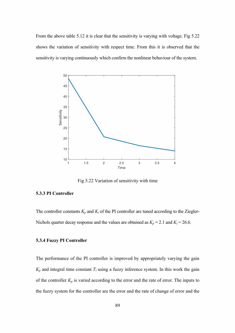
5.3.2 Sensitivity analysis ----------------------------------------------- 87

vii

5.3.3 PI Controller ------------------------------------------------------- 89


5.3.5 Modified Sliding Mode Controller ----------------------------- 91

5.3.6 Fuzzy SMC (FSMC) --------------------------------------------- 91

5.3.7 Optimization of Controller Gain using Krill Herd

Algorithm ---------------------------------------------------------- 92


5.4 Speed Control of Switched Reluctance Motor -------------- 101

5.4.1 Stability Analysis of the System ------------------------------ 102

5.4.2 PI Controller ----------------------------------------------------- 104

5.4.3 Fuzzy PI Controller --------------------------------------------- 104

5.4.4 Modified Sliding Mode Controller (SMC) ------------------ 105

5.4.5 Fuzzy SMC (FSMC) ------------------------------------------- 105

5.4.6 Results and Discussions --------------------------------------- 107

CHAPTER 6 NON-LINEAR INTELLIGENT CONTROL OF

AC DRIVES ---------------------------------------------- 113

6.1 Field Oriented Control of PMSM ---------------------------- 113

6.2 Stability Analysis of the System ------------------------------ 116

6.3 PI Controller ----------------------------------------------------- 118

6.4 Fuzzy PI Controller --------------------------------------------- 118

6.5 Modified Sliding Mode Controller (SMC) ------------------ 119

6.6 Fuzzy SMC (FSMC) ------------------------------------------- 119

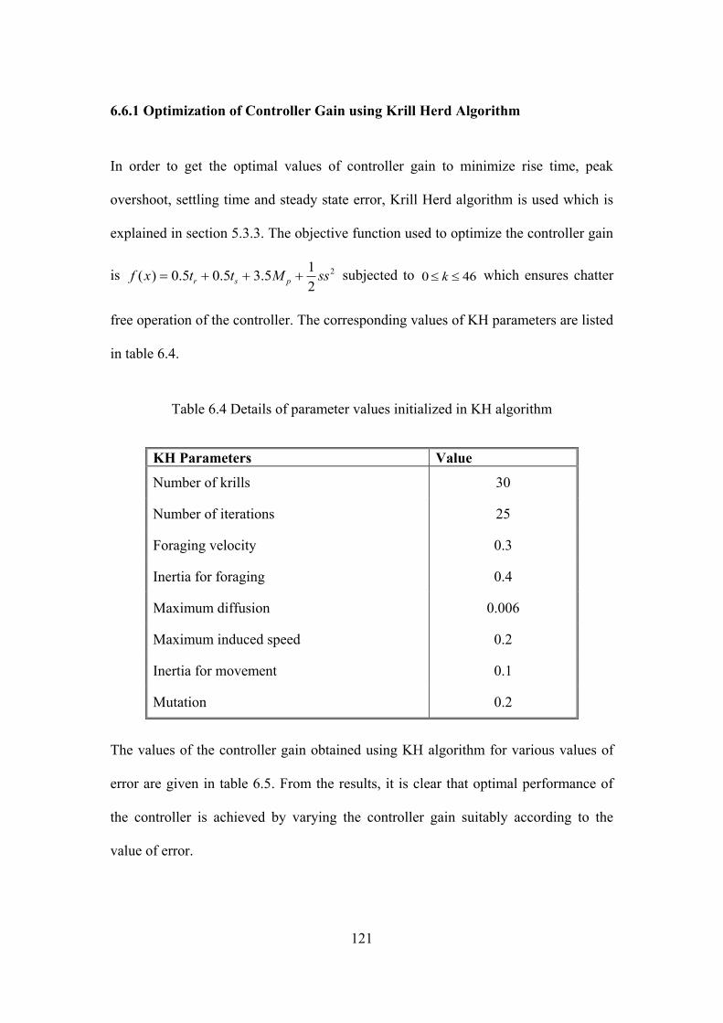
6.6.1 Optimization of Controller Gain using Krill Herd

Algorithm -------------------------------------------------------- 121

6.7 Results & Discussion ------------------------------------------- 122

CHAPTER 7 FPGA IMPLEMENTATION OF CONTROL

ALGORITHM IN INDUSTRIAL DRIVES -------- 128

7.1 Implementation of MATLAB and Simulink Algorithms

on FPGAs -------------------------------------------------------- 130

7.2 Implementation of Controller on FPGA --------------------- 131

7.3 Hardware in the loop Simulation ----------------------------- 132

7.3.1 Hardware in the loop (HIL) Simulation for the speed

control of PMSM ----------------------------------------------- 133

viii

7.3.2 Hardware in the loop Simulation for the speed control

of BLDC --------------------------------------------------------- 137

7.4 Hardware implementation of FSMC of BLDC ------------- 141

7.5 Result and Discussion ------------------------------------------ 142

CHAPTER 8 CONCLUSIONS AND FUTURE DIRECTIONS - 147

8.1 Conclusions ----------------------------------------------------- 147

8.2 Research Contributions ---------------------------------------- 152

8.3 Future Directions ----------------------------------------------- 153

REFERENCES ------------------------------------------------------------------ 154

LIST OF PAPERS SUBMITTED ON THE BASIS OF THIS THESIS -- 170

CURRICULUM VITAE

ix

LIST OF TABLES

Table Title Page No

Table 2.1 Evolution of Control Techniques ------------------------------------ 26

Table 3.1 Advantages and Disadvantages of DC Servo Motor -------------- 29

Table 3.2 Switching Sequence of BLDC Motor ------------------------------- 37

Table 3.3 Advantages and Disadvantages of BLDC Motor ------------------ 38

Table 3.4 Advantages and Disadvantages of SRM ---------------------------- 43

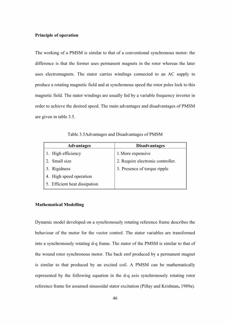
Table 3.5 Advantages and Disadvantages of PMSM ------------------------- 46

Table 4.1 Zeigler- Nichols Parameters for QDR Response ------------------ 52

Table 5.1 Parameters of DC Servo Motor -------------------------------------- 66

Table 5.2 Fuzzy Rules for FLC -------------------------------------------------- 69

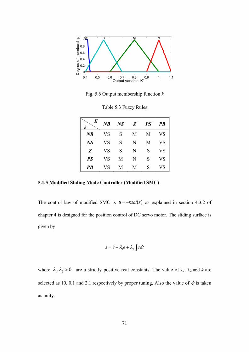
Table 5.3 Fuzzy Rules for Fuzzy PI --------------------------------------------- 71

Table 5.4 Fuzzy Rules for FSMC ------------------------------------------------ 73

Table 5.5 Comparison of Modified SMC and PI controllers ----------------- 75

Table 5.6 Performance comparison for the position control of DC servo

motor using various controllers -------------------------------------- 77

Table 5.7 Fuzzy Rules for Fuzzy PI Controller ------------------------------- 81


Table 5.9 Performance comparison for the speed control of DC servo

motor using various controllers -------------------------------------- 84

Table 5.10 BLDC motor parameters ---------------------------------------------- 85

Table 5.11 Variation of speed with voltage -------------------------------------- 87

Table 5.12 Sensitivity with change in voltage ----------------------------------- 88

Table 5.13 Fuzzy Rules for Fuzzy PI Controller -------------------------------- 90


Table 5.15 Parameter values initialized in KH algorithm ---------------------- 95

Table 5.16 Optimized values of controller gain --------------------------------- 97

Table 5.17 Performance comparison with various controllers --------------- 101

Table 5.18 Parameters of SRM --------------------------------------------------- 102


Table 5.20 Fuzzy Rules for FSMC ----------------------------------------------- 106

x

Table 5.21 Performance comparison with various controllers --------------- 110

Table 6.1 PMSM parameters ---------------------------------------------------- 116


Table 6.3 Fuzzy Rules for FSMC ----------------------------------------------- 120

Table 6.4 Details of parameter values initialized in KH algorithm -------- 121

Table 6.5 Optimized values of the controller gain --------------------------- 122

Table 6.6 Performance comparison with different controllers -------------- 125

Table 7.1 Comparison of HIL Simulation and Simulation (PMSM) ------- 136

Table 7.2 Comparison of HIL Simulation and Simulation (BLDC) ------- 141

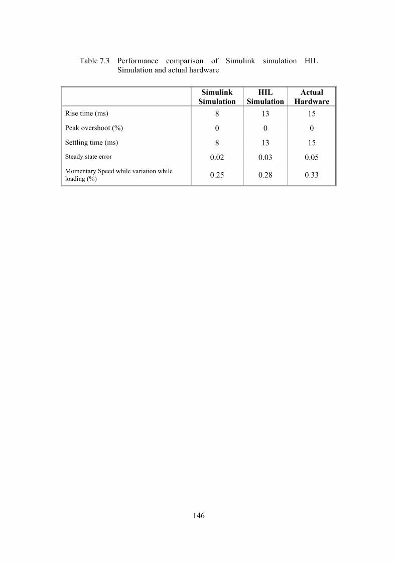
Table 7.3 Comparison of Hardware with Simulation Results --------------- 146

xi

LIST OF FIGURES

Figure Title Page

Fig. 3.1 Functional blocks of a drive system ----------------------------------- 27

Fig. 3.2 Structure of a DC servo motor ----------------------------------------- 31

Fig. 3.3 Motor toque with saturation -------------------------------------------- 33

Fig. 3.4(a) Structure of BLDC motor ---------------------------------------------- 35

Fig. 3.4(b) Cross section of BLDC motor ----------------------------------------- 35

Fig. 3.5 Circuit diagram of BLDC drive system ------------------------------ 36

Fig. 3.6 Ideal back EMFs, current and position sensor signals -------------- 37

Fig. 3.7 Structure of 3 phase 6/4 SRM------------------------------------------ 42

Fig. 3.8 Cross section of surface PMSM --------------------------------------- 45

Fig. 3.9 Equivalent circuit of PMSM ------------------------------------------- 47

Fig. 4.1 Open loop representation of a second order system ---------------- 55

Fig. 4.2 Block diagram of closed loop system -------------------------------- 56

Fig. 4.3 Phase- plane diagram of closed loop system for small s1 ---------- 56

Fig. 4.4 Phase- plane diagram of closed loop system for largel s1 ---------- 57

Fig. 4.5 Block diagram of a Fuzzy logic controller --------------------------- 61

Fig. 4.6 Block diagram of a Fuzzy SMC --------------------------------------- 64

Fig. 5.1 Block diagram of the position control of DC servo motor -------- 65

Fig. 5.2 Input membership functions for e and e ----------------------------- 69

Fig. 5.3 Output membership function ------------------------------------------- 69

Fig. 5.4 Surface view of fuzzy system ------------------------------------------ 70

Fig. 5.5 Input membership functions for e and e ------------------------------ 70

Fig. 5.6 Output membership functions ----------------------------------------- 71



Fig. 5.9 Step response with PI and conventional SMC in cyclic loaded

condition ------------------------------------------------------------------ 74

Fig. 5.10 Step response with PI and modified SMC at no-load --------------- 74

Fig. 5.11 Step response with PI and modified SMC in cyclic loaded -------- 74

Fig. 5.12 Step response with FLC and PI controller at constant load -------- 76

xii

Fig. 5.13 Step response with Fuzzy SMC, Fuzzy PI and PI controller at

constant load ------------------------------------------------------------- 77

Fig. 5.14 Block diagram of the speed control of DC Motor ------------------- 78





Fig. 5.19 Step response with Fuzzy SMC, Fuzzy PI and PI controller for

the speed control --------------------------------------------------------- 83

Fig. 5.20 Block diagram of BLDC speed control ------------------------------- 84

Fig. 5.21 Variation of speed with voltage --------------------------------------- 88

Fig. 5.22 Variation of sensitivity with time ------------------------------------- 89





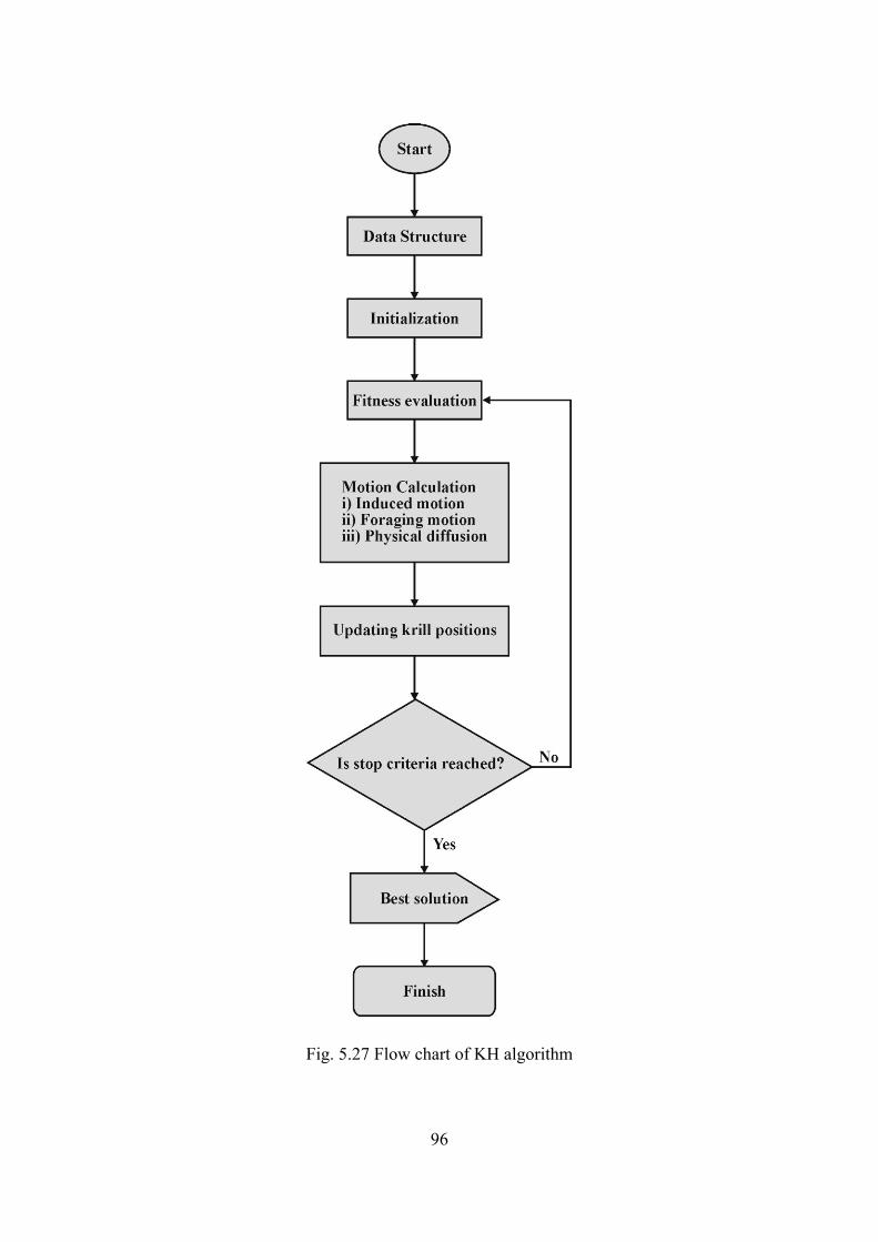
Fig. 5.27 Flow chart of KH algorithm -------------------------------------------- 96

Fig. 5.28 Step response of BLDC motor with Fuzzy SMC, SMC, Fuzzy

PI and PI controllers ---------------------------------------------------- 99

Fig. 5.29 Current in the three phases of BLDC motor ------------------------- 99

Fig. 5.30 Back EMF in the three phases of BLDC motor -------------------- 100

Fig. 5.31 Variation of speed and current with FSMC ------------------------- 100

Fig. 5.32 Block diagram of SRM speed control ------------------------------- 101


Fig. 5.34 Output membership functions ---------------------------------------- 104



Fig. 5.37 Step response of SRM with Fuzzy SMC and other controllers --- 109

Fig. 5.38 Response while loading with Fuzzy SMC and other controllers - 109

Fig. 5.39(a) Comparison of rise time of selected drives with FSMC,

Modified SMC, Fuzzy PI and PI controllers ------------------------ 110

xiii

Fig. 5.39(b) Comparison of peak overshoot of selected drives with FSMC,


Fig. 5.39(c) Comparison of settling time of selected drives with FSMC,


Fig. 5.39(d) Comparison of steady state error of selected drives with

FSMC, Modified SMC, Fuzzy PI and PI controllers -------------- 112

Fig. 6.1 Block diagram of the vector control of PMSM -------------------- 115





Fig. 6.6 Step response of PMSM with various controllers ------------------ 124

Fig. 6.7 Speed variation of PMSM under loaded condition ----------------- 124

Fig. 6.8 Speed and Current variation of PMSM with FSMC --------------- 125

Fig. 6.9 Comparison of performance indices of PMSM using FSMC,


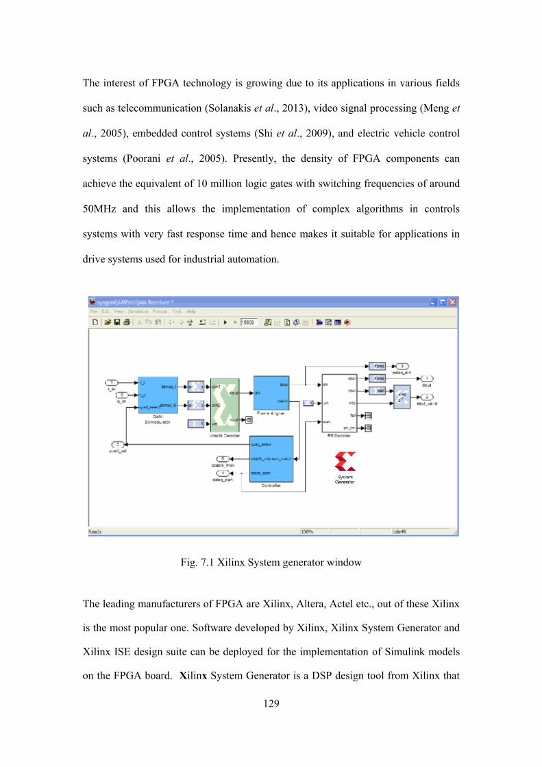
Fig. 7.1 Xilinx System generator window ------------------------------------- 129

Fig. 7.2 Arrangement for the hardware in loop simulation ----------------- 132

Fig. 7.3 Block diagram of FPGA implementation of Speed Control of

PMSM using FSMC ---------------------------------------------------- 134

Fig. 7.4 Step response of PMSM with FSMC using HIL simulation and

simulation --------------------------------------------------------------- 135

Fig. 7.5 Step response of PMSM with SMC using HIL simulation and

simulation --------------------------------------------------------------- 135

Fig. 7.6 Step response of PMSM with PI controller using HIL

simulation and hardware simulation --------------------------------- 136

Fig. 7.7 Block diagram of hardware implementation ------------------------ 139

Fig. 7.8 Step response of BLDC motor with FSMC using HIL

simulation and simulation --------------------------------------------- 139

Fig. 7.9 Step response of BLDC motor with SMC using HIL simulation

and simulation ---------------------------------------------------------- 140

Fig. 7.10 Step response of BLDC motor with PI controller using HIL

simulation and simulation --------------------------------------------- 140

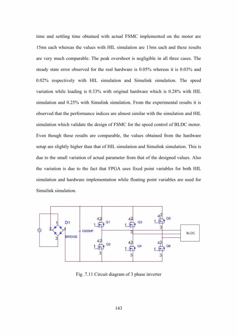
Fig. 7.11 Circuit diagram of 3 phase inverter ---------------------------------- 143

xiv

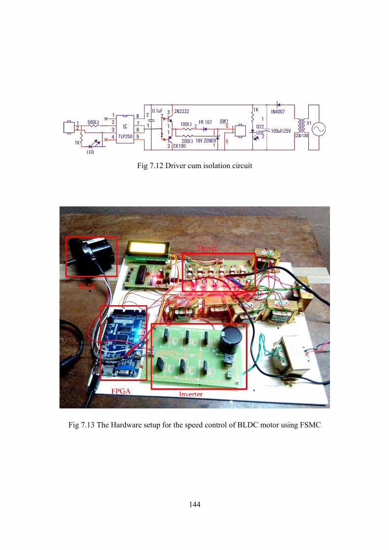
Fig. 7.12 Driver cum isolation circuit ------------------------------------------- 144

Fig. 7.13 The Hardware setup for the speed control of BLDC motor

using FSMC ------------------------------------------------------------- 144

Fig. 7.14 Step Response of Actual Hardware, HIL simulation and

Simulation --------------------------------------------------------------- 145

Fig. 7.15 Speed variation while loading with actual Hardware, HIL

simulation and Simulation --------------------------------------------- 145

xv

LIST OF ABBREVIATIONS

ACO - Ant Colony Optimization

ANFIS - Adaptive Neuro-Fuzzy Inference System

ANN - Artificial Neural Network

ASIC - Application Specific Integrated Chips

BLDC - Brushless DC Motor

DSP - Digital Signal Processor

EKF - Extended Kalman Filter

ELO - Extended Luenburger Observer

EV - Electric Vehicle

FIS - Fuzzy Inference System

FLC - Fuzzy Logic Controller

FPGA - Field Programmable Gate Arrays

FSMC - Fuzzy Sliding Mode Control

GA - Genetic Algorithm

HDL - Hardware Description Language

HEV - Hybrid Electric Vehicle

HIL - Hardware in the Loop

KH - Krill Herd

LQG - Linear Quadratic Gaussian

LQR - Linear Quadratic Regulator

MRAS - Model Reference Adaptive System

NB - Negative Big

NS - Negative Small

xvi

PB - Positive Big

PI - Proportional plus Integral

PID - Proportional plus Integral plus Derivative

PMSM - Permanent Magnet Synchronous Motor

PS - Positive Small

PSO - Particle Swarm Optimization

QDR - Quarter Decay Response

SMC - Sliding Mode Control

SRM - Switched Reluctance Motor

VHDL - Very High Speed Integrated Chip Hardware Description

Language

VSC - Variable Structure Control

Z - Zero

xvii

NOTATIONS

B Friction coefficient in N-m/rad/s

e(t) Error signal

ea , eb, ec Back EMF of BLDC in 3phases in V

Eb DC motor back emf in V

fa , fb , fc Trapezoidal functions

i Stator current of SRM in A

ia , ib, ic Input curents in 3 phases of BLDC motor in A

Ia Armature current of DC motor in A

id, iq Direct and quadrature components of stator current of PMSM in A

J Moment of inertia of the rotor in Kg-m2

K Gain constant of FSMC

Kb Back emf constant in V/rad/s

Kd Differential gain

Ki Integral gain

Kp Proportional gain

Kt Toque constant in N-m/A

L Stator inductance of SRM/PMSM in H

La Armature self-inductance of DC/BLDC motor in H

Ld, Lq Direct and quadrature components of stator inductance of PMSM in H

M Armature mutual inductance of BLDC motor in H

p differential operator

R Stator resistance of SRM/PMSM in ohm

Ra Armature resistance in ohm

s Seconds

xviii

s Sliding surface

sat Saturation function

sgn Signum function

T time

T Torque developed by DC motor in N-m

Te Electro-magnetic torque in N-m

Tl Load torque in N-m

u Control signal

V Stator voltage of SRM/PMSM in V

Va Armature voltage of DC motor in V

Va , Vb, Vc Terminal phase voltage of BLDC motor in V

vd, vq Direct and quadrature components of stator voltage of PMSM in V

Θ Angular position in rad

λ1, λ2 Constants of sliding surface

Φ Flux per pole in Wb

Φ Thickness of the boundary layer

Ψ or λp Flux linkage in Wb

ψd, ψq Direct and quadrature components of stator flux linkage of PMSM

in Wb

ψf Flux linkage due to permanent magnet in PMSM

ω Angular velocity in rad/sec

CHAPTER 1

INTRODUCTION

An electric drive is a power conversion means utilized by most of

the industrial automation systems and processes to convert electrical power to

mechanical power, and to control the torque, speed or position of the load. A modern

electric drive system consists of a motor, an electric converter and a controller

integrated together to perform a mechanical manoeuvre for a given load (Barrero and

Duran, 2016). Electric motors that are used in servo control applications for solar

tracking, antenna positioning, robotic arm movement, hybrid electric vehicles and

aerospace vehicles are some of the examples of special electric machines. Recent

developments in advanced manufacturing and automation in industries demand very

fast and robust techniques of characterization and control mechanisms of these

electric drives. Ultra precision and high speed machining are two major challenges

with great scientific relevance to meet the requirement of industrial automation (Rind

et al., 2017). Speed control of electric machines has become very fast and efficient

with the evolution of power electronic switches and various power converters that

help to convert and control electrical power from ac to dc, dc to dc, dc to ac as well as

ac to ac. DC Servo motors, Brush Less DC Motor (BLDC), Permanent Magnet

Synchronous Motor (PMSM) are some of the widely used special electric motors for

various industrial applications, viz. DC servo motor in traction, BLDC, PMSM and

Switched Reluctance Motor (SRM) motors in aerospace and electric vehicles(Bose,

2009). The basic criterion in selecting an electric motor for a particular application

depends on the power demand as well as characteristic performance during its steady

state and dynamic operations under no load as well as loaded conditions.

2

Characteristics of mechanical load, environmental factors and cost are also extremely

important factors that decide the selection of motor for its specific application. For

example, in applications like traction and elevators where high starting torque is

required, a DC series motor is a better choice than an induction motor where as in

petrochemical industries these motors are unsuitable as it produces sparking between

the brushes and commutator segments. Similarly PMSM find more promising

applications in Electric Vehicle (EV) / Hybrid Electric Vehicle (HEV) due to its

higher efficiency and lower rotor inertia even though they are more expensive than

induction motors (Rahman et al., 2006).

Drives are generally controlled by conventional Proportional – Integral – Derivative

(PID) controllers due to the advantages of its simple design, low cost, low maintenance

and their effectiveness. It is necessary to know the mathematical model of the drive

system or to setup some experiments for the tuning of PID parameters for its control.

However, it has been known that conventional PID controllers generally do not work

well for non-linear systems, particularly for complex and approximated mathematical

models (Pundaleek et al., 2010). Also, this control technique is not capable enough in

dealing with system uncertainties such as parameter variation and external disturbances.

A controller without D mode is preferred when large disturbances and noise are present

during the operation of the drive system. Subsequently alternate control mechanism

suitable for handling non-linearity in the system, machine parameter variations and load

variations are suggested. Recently developed control mechanisms like back stepping

control (Cai et al., 2017), adaptive control (Wai et al., 2015), H- infinity control (Zhou

and Hu, 2015) and Artificial Neural Network (ANN) based control (Ali et al., 2014) can

be used for the control and stabilization of systems with parameter uncertainty and

disturbances. Even though these controllers perform better than the linear controllers,

3

their algorithms are quite complex and computationally expensive which necessitates a

comparatively simple and effective controller for drive systems. Sliding Mode Control

(SMC), Fuzzy Logic Control (FLC) and their combination are found to be a better

solution from the point of view of design, implementation and economic considerations

for the control of drives.

SMC is a widely used method to handle uncertain non-linear systems (Young et al.,

1999). The main advantage of using SMC is that it is robust against external

disturbances and parameter variations (Decarlo et al., 1998). The control strategy in

SMC is designed such that the system states are directed and then constrained to lie on

a specified sliding surface or within a neighbourhood of a suitable switching surface as

long as the system trajectories stay on the surface. The closed-loop dynamics are

completely governed by the equations that define the surface (Spurgeon and Edwards,

1998). Conventional SMC has been successfully implemented to control drive systems

like DC motor (Dumanay et al., 2016) and BLDC motor (Chen et al., 2017) for the

control of position as well as speed. However for this SMC, the sliding surface uses a

discontinuous switching function resulting in chattering, a phenomenon of high

frequency oscillations in the output due to the high frequency switching of the control

action. The effect of chattering can be significantly reduced by boundary layer solution

(Lee and Utkin, 2007) in which, a boundary layer is introduced around the sliding

surface, which is achieved by replacing the discontinuous switching function with a

continuous form mostly by a saturation function. Performance of a chatter free SMC

using a continuous function with the gain made variable to adapt to the changes in load

as well as system parameters will definitely improve its performance. Fuzzy logic is an

effective method that can be used for varying parameters under certain rules.

4

Fuzzy Logic Controllers (FLC) that uses fuzzy set theory (Zadeh, 1965) expresses the

feedback control laws using heuristic knowledge, when parameters of the control

plants are unknown and is an effective tool to handle imprecise and uncertain

decision-making problems. FLC has been successfully applied to various industrial

control applications, such as speed control of DC motor (Montiel et al., 2007),

balancing of Ball and Beam system (Emhemed, 2013), vector control of Induction

motors (Uddin et al., 2002) etc. By combining the intelligence of Fuzzy logic with the

SMC, a considerable improvement in the controller output and thereby significant

enhancement in the system performance can be achieved (Baround et al., 2018).

FSMC is a combination of modified SMC and Fuzzy Inference system and it has been

successfully implemented in industrial applications like closed-loop vector control for a

grid-connected Wave Energy Conversion System (WECS) driven Self-Excited Induction

Generator (SEIG) (Elgammal, 2014), erection system with un-modelled dynamics (Feng

et al., 2017) and uncertain MIMO nonlinear systems (Roopaei et al., 2009)

BLDC motor is widely used in robotic arm movement where various linear as well as

nonlinear techniques are applied for its accurate position control (Camorali et al.,

2006). In order to achieve such precise control without overshoot and with fast

settling, a robust nonlinear intelligent controller is to be developed. Another key area

in which accurate speed control is essential is in electric vehicle where BLDC motor

and SRM are widely used. These motors are inherently nonlinear due to the presence

of variation in reluctance and magnetic saturation which results in coupled and

nonlinear dynamic system. Accurate speed control of the vehicle with continuously

varying load due to road condition can be accomplished with the use of a nonlinear

intelligent control method (Monteiro et al., 2015).

5

For the realization of any designed controller, both Application Specific Integrated

Chip (ASIC) and Field Programmable Gate Array (FPGA) provide a good solution.

An FPGA is a large-scale integrated circuit, for which the hardware configuration can

be changed by programming using Hardware Description Languages (HDL) like

VHDL (Very High Speed Integrated Chip HDL) and Verilog. Digital Signal

Processor (DSP) like ASIC is having predetermined, unchangeable hardware function

and hence computation of any complex controller like Fuzzy SMC becomes a

challenge using this. For the implementation of digital systems, FPGA is preferred

over ASIC due to the fast computational ability, configurable hardware construction,

low power consumption, embedded processor and shorter design cycle (Kung and

Tsai, 2007; Chou et al., 2013). FPGA is successfully used for the implementation of

aircraft control (Hartley et al., 2014), power generation control of hybrid power

system (Nagraj and Panigrahi, 2015) and in various similar servo applications.

Performance of a controller is normally evaluated using simulation software like

MATLAB based Simulink, Pspice or Psim. In the present research work the design

and simulation of the modified sliding mode controller, fuzzy controller and fuzzy

sliding mode controller for various DC and AC drives are carried out and their

performance is compared with that of Fuzzy PI and conventional PI controllers.

Hardware in the loop simulation (HIL) and actual hardware of the fuzzy sliding mode

controller using FPGA are also implemented. The performance of this actual

controller is compared with that of the simulation results for the validation purpose.

6

1.1 MOTIVATION FOR THE RESEARCH

Industrial drive systems are generally controlled by conventional Proportional –

Integral (PI) controllers.The main problem associated with the conventional linear PI

controllers is its inverse relationship between the speed of response and the peak

overshoot. The peak overshoot can be reduced only at the cost of speed of response or

the settling time of the system. Other linear controllers like Linear Quadratic Regulator

(LQR) and Linear Quadratic Gaussian (LQG) also exhibit the same problem and this

point towards the need of an alternate simple and economic technique suitable to

achieve better steady state as well as transient performance indices.

Non-linear and adaptive control methods have been applied to the speed and position

control of drive systems to overcome the problems associated with liner control

techniques. Back stepping control, Adaptive control, ANN control, FLC, SMC are

some of them. Of these, back stepping control lacks robustness and its practical

implementation is laborious due to its complex algorithm. Adaptive control gives

better performance when an accurate model is available. ANN is also a modern

intelligent control technique used mainly in robotic applications (Chaoui et al. 2009),

speech recognition (Kamble, 2016), pattern recognition (Basu et al. 2010) and many

more. Due to its limitation of training using algorithms, this method can lead to

variations in the output of the drive systems with very fast dynamic response and

sudden load variations. Fuzzy control is a better solution for intelligent control that

depends on heuristic rules even though it lacks a perfect mathematical model. On the

other hand it is found that parameter variation and external disturbances are dealt with

SMC and it is effectively used to eliminate the peak overshoot along with

7

improvement in the speed of response (Spurgeon and Edwards, 1998). The problem

associated with chattering in conventional SMC is reduced by modifying the control

law. The performance of modified SMC is further improved by intelligently varying the

controller parameters within an optimized range using a fuzzy inference system (FIS).

1.2 OBJECTIVES OF THE RESEARCH

The main objective of this work is to design, develop and implement non-linear

controllers of DC & AC drives suitable for the industrial applications with the

following properties.

Robust against machine parameter variation and external disturbances like

sudden load variation

Having high speed of response with reduced overshoot and steady state error

Less Complex and easy to design and implement

Economical

A conventional DC motor, SRM, BLDC motor and PMSM are considered for the

performance evaluation of various controllers. Hardware implementation of the most

suitable controller using FPGA on a BLDC motor, for the verification of design and

corresponding validation of results, is also the objective of this research work.

1.3 OUTLINE OF THE THESIS

The proposed thesis is organized in 8 chapters. The first chapter introduces the

problem and defines the aim of the thesis. Chapter 2 contains review of background

literature on various developments in linear and non-linear control techniques

8

especially for DC and AC drive systems. Chapter 3 explains various DC and AC

drives and their characteristics that make them applicable in different industrial

environment. This chapter includes the mathematical modelling of conventional DC

motor, BLDC motor, SRM and PMSM. Various linear and non-linear control

strategies used in drive systems are discussed in chapter 4. Chapter 5 presents the

design of controllers for position/speed control of DC servo motor, BLDC motor and

SRM. Design and performance analysis of FSMC, chatter free SMC, Fuzzy

controller, Fuzzy PI controller and conventional PI controller for these motors are

carried out in this chapter. Design of various controllers for AC motor is discussed in

chapter 6. FSMC, chatter free SMC, fuzzy PI controller and conventional PI

controller are designed for the field oriented control of a PMSM and their

performance comparison and analysis are carried out in this chapter.

The hardware implementation of the FSMC using FPGA is explained in chapter 7.

HIL Simulation of FSMC for PMSM and BLDC motor are carried out using Xilinx

Virtex 4 FPGA board and the results are analysed. The hardware implementation of

FSMC for the BLDC motor using FPGA is carried out and the results are validated in

this chapter. Chapter 8 concludes with a summary of the work done along with

suggestions for the future research.

CHAPTER 2

LITERATURE SURVEY

A brief review of existing modern industrial drives, linear control strategies, necessity

of non-linear controllers and advanced non-linear control techniques are discussed here.

2.1 MODELLING OF INDUSTRIAL DRIVES

An electric drive is an electromechanical device for converting electrical energy into

mechanical energy to impart motion to different machines and mechanisms for

various kinds of industrial applications. It is the workhorse in a variable-speed drive

system and is generally classified as dc and ac machines. Traditionally, ac motors,

particularly induction motors are used in constant-speed applications whereas DC

motors are widely used in variable-speed applications. A modern electric drive

system has a power source that supplies the energy, a converter which provides

adjustable voltage/current and/or frequency and a controller to ensure the stability as

well as the system performance (El-Sharkawi, 2000). The adjustable speed drive

constitutes a multivariable control system and therefore, in principle, the general

theory of multivariable control system is applicable. Here, the voltages and the

frequency are the control inputs and the outputs may be speed, position, torque, air gap

flux, stator current or a combination of these (Leonhard, 1984; Dong et al., 2018).

Mathematical model of a system is a set of equations to describe the behaviour of it and

is used for the simulation and analysis. Naresh K. Sinha et al. describes three different

mathematical models of an armature-controlled dc servo motor: (i) a precise nonlinear

10

model, (ii) a piecewise linear model, and (iii) a second-order linear model.

Experimental results are presented by comparing the various models, and a range of

applications for each is suggested (Sinha et al., 2018). A mathematical model of DC

servo motor used for the position control of a robotic arm is found in literature

(Benksik, 2004). The non-linear model incorporating the saturation effect of the core of

a DC motor for its speed control is found in (Mahajan and Deshpande, 2013). Also

non-linear modelling and identification of a DC motor rotating in two directions

together with real time experiments is demonstrated in (Kara and Eker, 2003).

A brushless DC (BLDC) motor model is explained by (Pillai and Krishnan, 1989b) in

which the motor has a trapezoidal back EMF, and rectangular stator currents to

produce a constant electric torque. State space model of BLDC motor for the

Simulink simulation of its speed control is described by (Muruganatham and Palani,

2010). Mathematical model of an inverter fed BLDC motor with PI control is

described by (Purnalal and Sunil Kumar, 2015). A BLDC motor with improved

magnetic material having high B-H product that is suitable for high power

applications is modelled by (Luk and Lee, 1994). A simplified model for simulation

and experimental analysis of BLDC motor suitable for sensor less operation is

explained by(Kaliappan and Chellamuthu, 2012). Here the technique of zero crossing

of back EMF is used to estimate the rotor position for the sensor less operation

instead of measuring it using Hall Effect sensors.

Iqbal Husain and Syed A. Hossain explain the modelling and control of switched

reluctance motor (SRM) including possible nonlinearities (Husain and Hossain,

2005). A novel model of SRM with C-core is explained by (Mao and Tsai, 2005).

11

This motor has the advantages of low-cost production that possesses high slot space

for ease of coil winding which can be used for high power applications. A simplified

model of IGBT inverter driven three phase 6/4 SRM used for variable speed pumping

is described by (Parker, 2004). A simple model of SRM with nonlinear magnetization

characteristics is used for computer-aided designs is described (Roux and Morcos, 2002).

(Pillai and Krishnan, 1989a) describes the dynamic d-q model for the vector control

of Permanent Magnet Synchronous Motor (PMSM). As the vector control transforms

the PMSM to an equivalent separately excited dc machine, the transfer function

between the electric torque and current is linear. Model for the direct torque control

(DTC) of PMSM is explained by (L. Zhong et al., 1997) and the simulation results

show that the torque response is much faster than the one with current control. A

PMSM is modelled and the motor parameters are optimized using genetic algorithm

for the performance improvement is carried out in (Shahat and Shewy, 2010). This

model can be used in various applications such as automotive, mechatronics, green

energy applications, and machine drives. A flux-weakening control for a current-

regulated surface mounted PMSM to obtain an extended speed range is demonstrated

in (sudhoff et al., 1995).

Mathematical modelling and speed/position control of various special electric motors

are also given by (Krishnan, 2001). A detailed survey of various existing linear as

well as non-linear control techniques is carried for the purpose of design and

implementation of an effective control strategy for the industrial drives.

12

2.2 LINEAR CONTROL TECHNIQUES

Proportional-integral-derivative (PID) controller is very widely used in many control

applications due to its simplicity and effectiveness (Ang et al., 2005). It is extensively

used in drive control applications such as speed control of DC motor (singh et al.,

2013), BLDC motor (Kumar et al., 2014), SRM (Nanda et al., 2016) and PMSM

(Chakravarthi and Karpagavalli, 2016). Even though the use of PID control has a long

history in the field of control engineering, the three controller gain parameters,

proportional gain KP, integral gain KI, and derivative gain KD, are usually fixed and

are obtained using the tuning process. The disadvantage of PID controller is its poor

capability in dealing with system uncertainty, i.e. parameter variations and external

disturbances. A very important step in the use of these controllers is the tuning

process which becomes complex due to its iterative procedure. Tuning a PID

algorithm generally aims to match some preconceived 'ideal' response profile for the

closed loop system. Many algorithms have been developed to guarantee the best

performance of the PID controller of which Ziegler-Nichols tuning method is the

most popular one (Wang et al., 1997; Lin and Jan, 2002; Yu and Hwang, 2004).

Another substitute to PID controller is the Linear Quadratic Regulator (LQR) for

which all the system states must be measurable, and its design methodology is

explained in detail by (Katsuhiko Ogata, 2002). If the system state variables are not

measurable, the alternative to LQR is the Linear Quadratic Gaussian (LQG) controller

in which all the state variables are estimated using a Kalman estimator and the

measuring noise is assumed to be Gaussian. Michael Athans, in his paper (Athans,

1971) has demonstrated the design philosophy of LQG controller based on

13

deterministic perturbation control, stochastic state estimation and linearized stochastic

control. The LQR and LQG design is also explained by (Stephani et al., 1998) and

Balazs Kulcsar in his paper discusses the fundamental aspects of LQR/LQG control

theory with an example of aircraft, controlled by a flight controller (Kulcsar, 2000).

The LQG controller design for balancing an Inverted Pendulum Mobile Robot is

described by (Eide et al., 2011).

2.3 NON- LINEAR CONTROL TECHNIQUES

Many dynamic systems behave as almost linear, under certain operating conditions

and therefore linear control theory is widely applicable in reality. But quite often,

when operating a system on its limits, different kinds of nonlinearities make them

self-known and may degrade the stability and performance properties to such an

extent that they are no longer acceptable. These nonlinearities must then be taken into

account while designing and implementing the controller for real time applications.

Different popularly used novel non-linear control techniques found in literature are

sliding mode control (SMC), back stepping control, gain scheduling and feedback

linearization of which SMC and back stepping are the most popular and are discussed

below. For analysing the stability of non-linear systems Lyapunov Stability criterion

and phase portrait methods are generally used (Slotine, 1991).

2.3.1 Sliding Mode Control (SMC)

SMC is a variable structure control (VSC) method which is explained by (Utkin, 1977;

Dracunov and Utkin, 1992). It is a nonlinear control method that alters the dynamics of

a nonlinear system by application of a discontinuous control signal which forces the

http://en.wikipedia.org/wiki/Nonlinear_control

http://en.wikipedia.org/wiki/Dynamic_system

http://en.wikipedia.org/wiki/Nonlinear_system

http://en.wikipedia.org/wiki/Discontinuous

14

system to "slide" along a cross-section of the system's normal behaviour. The state-

feedback control law is not a continuous function of time. Instead, it can switch from

one continuous structure to another based on the current position in the state space. The

most distinguished feature of VSC is that it is completely insensitive to parametric

uncertainty and external disturbances (Hung et al., 1993; Manjunath, 1995). The term

"variable structure control" arises because the controller structure around the plant is

intentionally changed by some external influence to obtain a desired plant behaviour or

response. The multiple control structures are designed so that trajectories always move

towards an adjacent region with a different control structure, and hence the ultimate

trajectory will not exist entirely within one control structure, instead, it will slide along

the boundaries of the control structures. The motion of the system as it slides along

these boundaries is called a sliding mode and the geometrical locus consisting of the

boundaries is called the sliding surface. The important feature of it is the relative

simplicity of design, control of independent motion (as long as sliding conditions are

maintained), invariance to process dynamics characteristics and external perturbations.

This means the system is insensitive to any variation or perturbation of the plant

parameters (Decarlo et al., 1988).

The main drawback of SMC is the phenomenon of chattering which produces high

frequency oscillations in the output due to the high frequency switching in the input.

V.I.Utkin et al. presented a guide to sliding mode control for practicing control

engineers. It offers an accurate assessment of the so-called chattering phenomenon

catalogues implementable sliding mode control design solutions and provides a frame

of reference for future sliding mode control research (Young et al., 1999). There are

many methods found in the literature to overcome the phenomenon of chattering and

http://en.wikipedia.org/wiki/State_space_(controls)

http://en.wikipedia.org/wiki/Feedback

http://en.wikipedia.org/wiki/Continuous_function

http://en.wikipedia.org/wiki/Locus_(mathematics)

15

one of the best solutions is to introduce a boundary layer around the switching surface

(Slotine and Sastry, 1983). The applications of sliding mode controller for electric

drives are also presented by (Utkin, 1993). A novel DC drive control scheme based

on the VSC theory has been proposed in (Damiano et al., 2004; Sarwer et al., 2004).

A sliding mode controller is designed and implemented for the speed estimation and

control of permanent magnet synchronous motor (Corradini et al., 2012) and a

chattering free SMC is realized for an electromechanical actuator with backlash

nonlinearity (Ma et al., 2017). A second order SMC algorithm, that reduces the effect

of chattering, is used to control a robust dc-drive which demands only rough

information about the actual motor parameters, is proposed by (Damiano et al., 2004).

The design of a PI-Sliding Mode controller for the speed control of an induction

motor used for electric vehicle is explained and the results are compared with that of

conventional SMC and PI controller by (Ltifi et al., 2014). Speed control of an

electromechanical system using back stepping integral sliding mode controller

(BSISMC) is implemented and its performance in the presence of uncertainties and

disturbances is compared with that of conventional SMC and the results indicate

robust performance with good tracking ability (coban, 2018).

2.3.2 Back stepping control

Back stepping is a novel non-linear design technique for non-linear systems where the

useful nonlinearities are not cancelled in the design process. It is a Lyapunov method

based versatile nonlinear control design approach that is particularly well suited for

addressing the problem of multivariable control problem of complex nonlinear

systems developed by (Kokotovic et al., 1995) for a special class of dynamical

http://en.wikipedia.org/wiki/Dynamical_system

16

systems. This technique focuses on breaking down the complex nonlinear systems

into smaller subsystems for the design of Lyapunov functions for the control. The

virtual control for these subsystems is obtained by integrating the individual

controllers into an actual controller by stepping back through the sub system and re-

assembling it from its component subsystems (Joseph and Geetha, 2007). Because of

this recursive structure, the designer can start the design process at the known-stable

system and "back out" new controllers that progressively stabilize each outer

subsystem. The process terminates when the final external control is reached and

hence is known as back stepping control.

Back stepping control is applied for the stabilization of permanent magnet

synchronous motor (Merzoug, 2010) and linear induction motor (Hasirci et al., 2009;

Bousserhane et al., 2009). A model reference adaptive estimator with back stepping

control is used for the control of induction motor (Mehazzem et al., 2009), brushless

DC motor (Lin et al., 2009a) and interior permanent magnet (IPM) synchronous

motor (Lin et al., 2009b; Lin et al., 2011a). Adaptive back stepping with PI sliding

mode position control for synchronous reluctance motor drives is found in (Lin et al.,

2011b). A comparison between chaos synchronization using active control and back

stepping control is also found in (Vincent, 2008).

2.4 SOFT COMPUTING TECHNIQUES IN CONTROL

Soft-Computing is a collection of techniques spanning many fields that fall under

various categories in Computational Intelligence and Fuzzy Logic, Neural Networks

and Evolutionary Computation are three main branches of it. Soft computing deals

with imprecision, uncertainty, partial truth and approximation to achieve practicability,

robustness and low solution cost.

http://en.wikipedia.org/wiki/Dynamical_system

http://en.wikipedia.org/wiki/Recursion

17

2.4.1 Fuzzy Logic

Fuzzy logic is an approach to computing based on "degrees of truth" rather than the

usual "true or false" (1 or 0) Boolean logic on which the modern computer is based.

The idea of fuzzy logic was first advanced by Dr.Lotfi A. Zadeh of the University of

California at Berkeley in the 1960s (Zadeh, 1965). Fuzzy logic not only includes 0

and 1 as extreme cases of truth (or "the state of matters" or "fact") but also the various

states of truth in between. For example, the result of a comparison between two things

could be not "tall" or "short" but "0.38 of tallness". Fuzzy logic seems closer to the

way our brains work. Fuzzy theory is extensively used for the control of dynamic

plant and process control applications (Mamdani, 1974; Jang et al., 1997).

Fuzzy logic is used along with conventional controllers to encounter actuator

saturation has been reported earlier in the literature (Gharieb and Nagib, 2001), in

which ‘I’ term of PID controller is nullified in order to prevent integrator windup. A

comparison of fuzzy controller with a PID controller for the control of a DC motor is

explained in (Sousa and Bose, 1994) and the design of a fuzzy PID controller is

proposed in (Upalanchiwar and Sakhare, 2014). Sliding mode speed control and

fuzzy torque control of IPM synchronous motor (Abianeh, 2011), fuzzy gain

scheduling of PID controller (Vijamaa, 2002; Zhao et al., 1993) are also found in

literature. Fuzzy logic control when used for the speed control of BLDC motor gives

better adaptability compared to conventional PI controller and offers improved

transient as well as steady state performance (Usman and Rajpurohit, 2014). The

SRM drive with the angle position closed-loop speed control based on fuzzy logic

shows good dynamic performance and high efficiency (Chen et al., 2002).

http://searchcio-midmarket.techtarget.com/definition/Boolean

18

2.4.2 Artificial Neural Net work

Neural network controllers have emerged as a tool for difficult control problems of

unknown nonlinear systems and are used for modelling and control of physical systems

due to their ability to handle complex input-output mapping without detailed analytical

models (Haykins, 1999). The application of Neural Network for the speed control of DC

motor (Minkova et al., 1998; Nouri et al., 2008] and gain scheduling (Tan et al., 1997)

are found in literature. A wavelet-neural network can also be used along with sliding

mode controller (El-Sousy, 2011) for the PMSM drives for its speed control. Recently

much research has been done on the applications of fuzzy neural network (FNN)

systems, which have the advantages of both fuzzy systems and neural networks, in the

control fields to deal with nonlinearities and uncertainties of the control systems (Cirstea

et al., 2002). Moreover, the FNN’s are universal approximators which can approximate

any dynamics to a pre-specified accuracy by the learning process. Back stepping FNN

controller combines the advantages of the back stepping control with robust

characteristics and FNN with on-line learning ability for the accurate speed control of

PMSM (Lin and Lin, 2009). Optimum position control of a BLDC motor is achieved

using PID controller and the estimation of the mechanical parameters at various load

setting as well as PID parameters are carried out using ANN (Ganesh et al., 2012).

2.4.3 Genetic Algorithm

Genetic Algorithm (GA) is a soft computing technique used for optimization of

controller parameters, based on natural selection, a process that drives the biological

evolution (Chaiyaratana and Zalzala, 1997). The use of genetic algorithm for the

19

tuning of a PID controller is proposed in (Lin et al., 2003) for the speed control of

linear model BLDC motor and a GA tuned PI controller is used for the vector control

of PMSM (Kuntol and Seok-kwon, 2013) and induction motor (Dey et al., 2009).

2.5 ADAPTIVE CONTROL

Adaptive Control is used for system with parameter variation and uncertainties and

this controller can modify the systems behaviour in response to changes in the

dynamics of the process and character of the disturbances. For example, when an

aircraft flies, its mass will slowly decrease as a result of fuel consumption and the

control law has to adapt itself to such changing conditions. The adaptive control

systems are mainly classified in to three categories namely Gain scheduling, Model

Reference Adaptive Control (MRAC) and Self tuning regulators (STR) (Astrom and

Wittenmark, 1997). Gain scheduling is an approach to control of non-linear systems

that uses a family of linear controllers, each of which provides satisfactory control for

a different operating point of the system (Lawrence and Rugh, 1995). Model

Reference Adaptive Systems (MRAS) may be regarded as an adaptive control

technique in which the desired performance is expressed in terms of a reference

model, which gives the response to the command signal. MRAC technique is found to

be used for the speed control of a BLDC motor (Bernat and Stepien, 2011) and the

design of a Model Reference Adaptive Controller using modified MIT rule for a

Second Order System is explained (Jain and Nigam, 2013). In Self tuning regulators,

the process parameters are estimated in real time and the controller parameters are

varied according to the process parameters and the algorithm and applications of STR

is explained by (Astrom et al., 1977). The use of STR for the tracking control of a DC

servo motor is explained in (Khamis, 2013).

http://en.wikipedia.org/wiki/Non-linear_system

http://en.wikipedia.org/wiki/Controller_(control_theory)

20

2.6 ROBUST CONTROL

Robust control originates with the need to cope with systems that has modelling

uncertainty and these methods aim to achieve robust performance in the presence of

bounded modelling errors. Most popular robust control techniques are H-infinity

control and μ- synthesis. A robust H-infinity optimal speed control scheme for a DC

motor with parameters variations and disturbance torque using a linear matrix

inequality (LMI) approach is presented in (Lu et al., 2008) and an H-infinity

controller design for permanent-magnet DC motor is proposed in (Brezina and

Brezina, 2011). A μ synthesis controller design method for a DC-motor-based active

suspension is described by (Zhang et al., 2012).

2.7 SENSOR LESS CONTROL

Sensor less control is used in drive system where the measurement of speed/ position

using sensors is difficult and in such cases, several rotor speed and position

estimation techniques have been applied. The back-EMF based rotor speed estimation

method works satisfactorily at higher speeds. However, the speed estimation becomes

very difficult at lower speeds, due to the small values and distorted EMF signal. State

observer methods based on Extended Kalman Filter (EKF) (Bolognani et al., 2003),

Extended Luenburger Observer (ELO) (Li and Zhu, 2008), and Sliding Mode

Observer (Li and Elbuluk, 2001) are used for the speed estimation of PMSM. Most of

these methods suffer from complex computation, sensitivity to parameter variation

and need of accurate initial conditions. The EKF has the advantage of estimating the

parameters and speed simultaneously by considering them as state. However, it is

21

computationally extensive and requires a high sampling frequency so that a simple

discrete-time equivalent model can be used. The sliding mode observer is simple and

offers a limited robustness against the parameter variation. However, sliding mode

being a discontinuous control with variable switching characteristics has chattering

problems and it may affect the control accuracy. Recently, some more advanced

adaptive estimation techniques based on Artificial Neural Network (ANN) (Batzel

and Lee, 2000; Liu and Wang, 2006) and Fuzzy Logic Control (FLC) (Adam and

Gulez, 2008) have also been reported for the speed estimation of PMSM. However,

the estimation accuracy depends on number of neurons and number of fuzzy

membership functions used for rule base and requires off-line tuning. One of the

recent speed estimation techniques is Model Reference Adaptive System (MRAS)

which is based on the adaptive control (Liang and Li, 2003). MRAS method uses two

models one independent of rotor speed (Reference Model) and the other dependant on

rotor speed (Adjustable Model), both having same output. The error of these actual

and estimated outputs is fed to the adaptation mechanism that outputs the estimated

rotor speed. This estimated value of speed is used to tune the adjustable model till

error is zero where the estimated speed is equal to the actual speed. MRAS method

suffers from parameter dependence and pure integrator related problems in reference

model. To overcome this problem, an alternative MRAS structure along with

Adaptive Neuro-Fuzzy Inference System (ANFIS) is used in PMSM motor (Jain et

al., 2011) which is again facing the problem of computational complexity. From the

literature it is found that some of the speed/ position estimation techniques have

several limitations while some others are computationally complex. Also it is required

to use sensors to measure the other state variables such as voltage and current in order

22

to estimate the speed/ position. Due to these disadvantages it is better to use the speed

/position sensors in applications where their use is not limited due to the

environmental conditions.

2.8 FUZZY SLIDING MODE CONTROL

By combining the intelligence of Fuzzy logic with SMC, a considerable improvement

in the controller performance can be achieved. This method has been successfully

implemented for the air flow control of a fuel cell (Baround et al., 2018), closed-loop

vector control for a grid-connected Wave Energy Conversion System (WECS) driven

Self-Excited Induction Generator (SEIG) (Elgammal, 2014), erection system with un-

modelled dynamics (Feng et al., 2017), and to handle uncertain MIMO nonlinear

systems (Roopaei et al., 2009). A two dimensional fuzzy sliding mode control of a

field-sensed magnetic suspension system is given in (Li and Chiou, 2014) and FSMC

with low pass filter in order to reduce chattering is given in (Balamurugan et al., 2017).

2.9 OPTIMIZATION OF THE CONTROLLER GAIN

Optimization can be defined as the act of achieving the best possible solution to

problem under given circumstances. In recent years, meta-heuristic algorithms have

been widely used for solving optimization tasks and are proven to be efficient when

compared to the other conventional methods based on the Linear and Non-Linear

programming. The main advantage of these algorithms is the avoidance of local

minima and the other benefits are simplicity, flexibility and derivation free structure

(yang, 2010). Some of the popular meta-heuristic algorithms are as follows. Genetic

algorithm (GA) is one of the evolutionary search algorithms, which was proposed by

23

Holland in 1967 based on Darwinian evolution of survival of the fittest that uses

crossover and mutation as two operators (Holland, 1967). Simulated annealing is

another example which is inspired by annealing process of melts, proposed in 1983

(Kirkpatrick et.al., 1983). Particle Swarm Optimization (PSO) proposed by Kennedy

and Eberhart in 1995 in which the particles sharing the information of the best position

they ever found to find the global optimal (Eberhart and Kennedy, 1995). Ant Colony

Optimization (ACO) proposed by Dorigo et al. in 1996 inspired by the behaviour of

ants in nature in finding the nearest path between their nest and the food source (Dorigo

et al., 1996). Differential evaluation is proposed by Storn and Price in 1997 (Storn and

Price, 1997) and Bees Algorithm proposed by Pharm et al in 2005 (Pharm et al., 2005)

is a swarm-based optimization algorithm that mimics the food foraging behaviour of

honey bees. Optimizing the parameters of a PID controller using meta-heuristic

methods like Genetic Algorithm (GA), particle swarm optimization (PSO) and the

method of cross entropy (CE) for process control application is described in (Mora, et

al., 2016). An efficient algorithm based on Ant colony optimization (ACO) applied for

the parameter optimization of PID controller for DC motor speed control which can

preferably conquer the shortcomings of traditional optimization methods and efficiently

improve the global convergence speed is described in (Ibrahim et al., 2014). PSO is

applied for the parameter optimization of an H- infinity controller for the control of a

pneumatic servo actuator (Ali et al., 2010).

One of the recent bio-based swarm intelligence algorithms, called Krill Herd (KH),

proposed by Gandomi and Alavi in 2012 by idealizing the swarm behaviour of krill

(Gandomi and Alavi, 2012; Wang et al., 2014). For the krill movement, the objective

function used in KH is determined by the least distances from food and the highest

24

herd density. By idealizing the swarm behaviour of krill, KH is a meta-heuristic

optimization approach for solving optimization problems. In KH, the position of Krill

is mainly affected by three actions, namely movement affected by other krill, foraging

action and physical diffusion. Comparing with other algorithms, one of the

advantages of the KH algorithm is that it requires only few control variables to

regulate. An optimal PID controller is designed for the frequency oscillation damping

of a wind-diesel hybrid system using Krill Herd (KH) algorithm by Shayanfar et al. in

(Shayanfar et al., 2015). In the present study, it is aimed to optimize the gain of Fuzzy

SMC controller based on Krill Herd Algorithm to control the speed with optimum

performance. The controller gain is optimized by using an objective function based

on improvements of parameters such as rise time, maximum overshoot, settling time

and minimum steady state error.

2.10 HARDWARE IMPLEMENTATION OF THE CONTROLLER

For the real time application of any controller its realization using a suitable processor

is essential. When, the model incorporating various system nonlinearities in the

presence of modelling error, disturbances and noise, an embedded processor capable

of fast computational ability and high switching speed, is required for its

implementation. Application Specific Integrated Chip (ASIC) like digital signal

processor (DSP) and field programmable gate array (FPGA) are the popularly used

processors for the realization of complex control algorithms. Implementation of a PI

controller for the speed control of an induction motor drive using DSP processor is

explained in (Mohznty and Muthu, 2011). However DSP operates in the KHz range

and becomes unsuitable when used for embedded applications with higher switching

frequency (Li, et al., 2011). Moreover, DSP has the limitation of fixed hardware

25

configuration that makes it application specific and hence FPGA with programmable

hardwired feature, fast computation ability, shorter design cycle, embedding

processor, low power consumption and higher density is preferred for the

implementation of the digital controllers (Kung and Tsai, 2007; Chou et al., 2013). A

review of the state of art of FPGA design methodologies with a focus on industrial

control system applications is suggested in (Monmasson and Cirstea, 2007). Design

and implementation of PID controller based on FPGA for low voltage synchronous

DC to DC buck converter is described in (Chnader et al., 2010). The effectiveness of

a FPGA based lag-lead compensator for the position control of a CNC machine is

explained in (Osornio-Rios, 2017). FPGA implementation of SMC is found in many

literatures, viz. Voltage control of a DC-DC Single-Ended Primary Inductor

Converter (SEPIC) (Li, et al., 2011) and the position control of a robot manipulator

(Piltan et al., 2015; Piltan et al., 2011). Also an FPGA based adaptive back stepping

sliding-mode controller is proposed to control the mover position of a linear induction

motor (Lin et al., 2007). The implementation of fuzzy logic controller for the speed

control of electric vehicle with DC motor using FPGA is given in (Poorani et al.,

2005) and an improved adaptive fuzzy logic speed controller for a DC motor, based

on FPGA implementation is proposed in (Ramadan et al., 2013). Moreover the design

of the Fuzzy-PI controller for omnidirectional robot navigation system and its

hardware implementation using FPGA is explained by (Masmoudi et al., 2016).

Here we aim to analyse the suitability of Fuzzy SMC for the speed control of selected

industrial drives under real time conditions of parameter variation and external

disturbances. For this purpose modelling of DC servo motor, BLDC motor, SRM and

PMSM are designed incorporating their important nonlinearities.

26

The development of various control techniques used for different drive system as

given in literature are summarised in table 2.1

Table 2.1 Evolution of Control Techniques

Linear

Control

Techniques

Nonlinear

Control

Techniques

Robust Control

Techniques

Intelligent

Control Using

soft computing

Adaptive Control

PID (1922)

LQR/ LQG

(1972)

SMC (1977)

Back stepping

(1990)

H infinity (1978)

Mu synthesis

(1995)

Fuzzy Logic(1965)

ANN (1954)

Genetic Algorithm

(1970)

STR(1978)

MRAC (1978)

CHAPTER 3

MODELLING OF DC AND AC DRIVES

An electric drive is a power conversion means utilized by most of

the industrial automation system and process to convert electrical power to

mechanical power. Speed, position and torque control are the major functions of an

electric drive in industrial applications.

A modern electric drive system has five main functional blocks, a power source, a

converter, a motor, a controller and a mechanical load as shown in fig 3.1. The power

source provides the energy required for the drive system. The converter interfaces the

motor with the power source and provides the motor with adjustable voltage/current

and/or frequency. The controller supervises the operation of the entire system to

enhance overall system performance and stability (El-Sharkawi, 2000).

Fig 3.1 Functional blocks of a drive system

The electric motor is the electro-mechanical energy conversion device which acts as

the work horse of the drive system whose speed/position and torque is to be

controlled in such a way that it matches with the application requirement. In order to

28

achieve the desired performance of the motor, an electronic converter along with a

suitable controller is employed. The most basic function of the controller is to

monitor the system variables, compare them with some desired values and readjust

the converter output until the system achieves the desired performance and this

feature is used in speed or position control applications in electric drives. The

controller is also used to enhance the stability of the system. For the design of a

controller, a suitable mathematical model represented by a set of equations that

describe the behaviour of the system and provides the complete specification of the

real drive is required.

Drives are broadly classified into two categories, namely DC and AC according to the

nature of the power source used. Traditionally DC drives are used for variable speed

applications where as AC drives are used for constant speed applications.

Conventional DC motors, Brushless DC Motor (BLDC), Permanent Magnet

Synchronous Motor (PMSM) are very widely used for various industrial applications,

viz. conventional DC motor in traction, BLDC, PMSM and Switched Reluctance

Motor (SRM) motors in aerospace and electric vehicles (Rind et al., 2017). The basic

criterion in selecting an electric motor for a particular application depends on the

power demand as well as characteristic performance during its steady state and

dynamic operations under no load as well as loaded conditions. Characteristics of

mechanical load, environmental factors and cost are also extremely important factors

that decide the selection of motor for its specific application. For example, in

applications like traction and elevators where high starting torque is required, a DC

series motor is a better choice than an induction motor where as in petrochemical

29

industries these motors are unsuitable as it produces sparking between the brushes

and commutator segments. Similarly PMSM find more promising applications in

Electric Vehicle (EV) or Hybrid Electric Vehicle due to its higher efficiency and

lower rotor inertia even though they are more expensive than induction motors

(Rahman et al., 2006).

3.1 DC DRIVES

DC drives are the electro-mechanical power converters that use DC power as the

source of energy. Commonly available DC motors are conventional DC motor,

BLDC motor and Switched Reluctance Motor (SRM). In the present chapter the

mathematical modelling incorporating their important nonlinearities are carried out.

Table 3.1 Advantages and Disadvantages of DC motor

Advantages Disadvantages

1. Very precise speed and position

control

2. Wide range of speed and torque

3. More powerful than permanent

magnet motors

1. Sparking in commutator results in

reduced brush and commutator life

2. High maintenance cost

3. Require more current than permanent

magnet motors

3.1.1 DC Servo motor

DC motor plays a significant role in modern industry due to their simple, effective

and wide range of provision for speed and position control (Tripathi et al., 2013).

Numerous applications that demand good speed control with high accuracy and fast

dynamic responses are in various fields’ viz. rolling mills, pulp and paper mills,

30

cranes, hoists, elevators, machine tools, transit system and locomotive drives

(Leonard, 1984). Various advantages and disadvantage of a conventional DC servo

motors are given in table 3.1.

Mathematical Modelling of a DC Servo Motor

The general approach in mathematical modelling of a DC motor is to neglect the

nonlinear effects due to the magnetic saturation and friction and build a linear transfer

function representation for the input–output relationship of the motor and the load it

drives. Some of the electromechanical systems driven by DC motor exhibits nonlinear

behaviour, because of the motor saturation, friction and quantization noise in the

measurement sensors. In the presence of these non-linear behaviours, it is difficult to

use a linear controller as the nonlinear effects need not predict and vary according to

the plant load as expected. Under such circumstances, the modelling of the machine

and their linear control strategies often fails to work in the real world system.

The electric circuit of the armature and the free body diagram of the rotor are shown

in fig. 3.2. Depending on the application, the speed/position of a DC motor is

controlled by varying the input voltage or field current. The desired speed is tracked

according to the shaft position of the motor and is determined by a reference signal

using a suitable controller. This controller is selected so that the error between the

system output and reference signal corresponding to the desired position and/or speed

eventually tends to its minimum value, ideally zero.

31

Here the variation of input voltage is used as the control parameter for the position

control of the motor. A constant dc voltage is selected as a reference signal to obtain

the desired position of the motor. However, the method works successfully for any

reference signal, particularly for any stepwise time-continuous function, that may be a

periodic signal to get a desired shaft position, with desired angle between 0 and 360

degrees from a virtual horizontal line.

Fig.3.2 Structure of a DC Motor

The dynamics of a linearized DC servo motor is given in equations (3.1) to (3.5)

ba

aaaa Edt

dILIRV (3.1)

LTBdt

dJT

(3.2)

ata IKIKT (3.3)

bb KE (3.4)

dt

d (3.5)

32

Where Ra is armature resistance [Ω], La is armature self-inductance [H], Va is the

armature voltage [V], Ia is the armature current [A], Eb is the motor back emf [V], T

is the torque developed [N-m], TL is the load torque[N-m], J is the moment of inertia

of the rotor[kg·m2], B is the friction coefficient[N-m/rad/s], Φ is the flux per pole

[wb], Kt is the toque constant[N-m/A], Kb is the back emf constant[V/rad/s], ω is the

angular velocity[rad/sec] and θ is the angular position[rad].

From the above equations, the state variable model of DC motor at no-load (TL=0)

and loaded condition are given by eqs. (3.6) and (3.7) respectively

a

aa

t

b

b

a

a

a

V

LI

J

B

J

K

L

K

L

R

I

0

0

1

010

0

0

(3.6)

a

aa

t

b

b

a

a

a

VJ

LI

J

B

J

K

L

K

L

R

I

00

10

01

010

0

0

(3.7)

The corresponding output equation is

aI

Y 100

(3.8)

33

Where Y is the position of the motor

Even though the machine normally operates in the linear range of its characteristics

where the saturation effect is neglected, under certain conditions like high starting current

and overloaded states this becomes very significant and adversely affect the accuracy of

the output. Without considering the effect of magnetic saturation, electrical torque

represented by eq. (3.3) will be lower than the expected value due to the armature

reaction that distorts the flux in the air-gap resulting in a nonlinear torque function.

Another significant nonlinearity present in the DC motor is the Coulomb friction. Stiction

(or starting friction) is the amount of force required to start the relative motion and is

greater than the amount required to sustain it. However the effect of Coulomb friction is

significant only at extremely low speeds and hence magnetic saturation is considered as

more predominant nonlinearity in an electric motor. The block diagram of the system

considering the effect of magnetic saturation is shown in fig 3.3.

Fig.3.3 Motor torque with saturation

Considering the effect of magnetic saturation, eq. (3.3) is modified as

)( atIKsatT (3.9)

The complete state model incorporating the nonlinearity due to magnetic saturation

under loaded condition is

34

L

a

aa

t

b

b

a

a

a

T

V

J

LIsat

J

B

J

K

L

K

L

R

I

00

10

01

)(

010

0

0

(3.10)

3.1.2 Brushless DC Motor (BLDC)

BLDC Motors are popularly used in many applications such as automotive,

computers, aerospace, medical, industrial automation equipment and instrumentation

(Mathew and Caroline, 2013). They have several advantages over brushed DC motor

such as lower maintenance due to the elimination of the mechanical commutator and

high power density which makes them ideal for high torque to weight ratio

applications (Luk and Lee, 1994).

Modern brushless motors are very similar to ac motors. A permanent Magnet AC motor

with a trapezoidal back EMF is referred to as BLDC motor and those with sinusoidal

back EMF is referred as permanent magnet synchronous motor (PMSM). The brushes

and commutator are eliminated in BLDC motor and it has a rotor with permanent

magnets and a stator with windings that are connected to an electronic commutator which

energizes the windings with particular sequence of switching pulses.

The structure of a typical three-phase brushless dc motor is illustrated in fig.3.4 (a)

and (b). The stator windings are similar to those in a poly phase ac motor, and the

rotor is composed of one or more permanent magnets. Brushless DC motors are

different from AC synchronous motors where, the former incorporates some means

for detection of rotor position (or magnetic poles) to produce signals to control the

35

electronic switches (Puranalal and Kumar, 2015) where as in AC synchronous motor,

there are no position sensors and the rotor poles are magnetically locked with the

stator poles to continue the rotation. The BLDC motor operates either with sensors or

without any position sensors. When it operates with sensor, three Hall Effect sensors

are employed for sensing the rotor position whereas in sensor less operation the rotor

position is estimated from the back EMF. The Hall Effect sensor is a transducer that

varies its output voltage in response to the magnetic field.

Fig 3.4 (a) Structure of BLDC motor Fig 3.4(b) Cross section of BLDC motor.

Principle of Operation

The stator windings are energized in a predefined sequence in such a way that they

lead the rotor magnets and switches so that the rotor aligns with the stator and by this

continuous operation the motor rotates. The motor runs in the opposite direction by

reversing the sequence. The sequence defines the direction of the current flow in the

coils that determines the orientation of the magnetic field generated by the coil. The

equivalent circuit of the stator of BLDC motor is similar to that of an AC motor with

star connection. The stator is fed from a DC source through an electronic converter

which acts as the electronic commutator. The circuit diagram of a three phase BLDC

motor is shown in fig 3.5

36

Three phase BLDC motor is operated by switching on two phases at a time. The

signals from the Hall Effect position sensors produce a three digit number which

changes at every 60 electrical degrees. These switching signals and the ideal back

EMF and current waveforms are shown in fig 3.6. Table 3.2 shows the switching

sequence, current direction and the position sensor signals.The voltage is applied to

each of the three stator winding for a duration of 120° electrical in each cycle with a

current limit to hold the stator current with in the motor capabilities, which results in

trapezoidal or quasi-rectangle shaped currents in the stator windings. Because the

phase currents are excited in synchronism with the constant value of the back EMF,

constant torque is generated. The electromagnetic torque of the BLDC motor is

proportional to the product of phase values of back EMF and current. The back EMF

in each phase is trapezoidal in shape and is displaced by 120 electrical degrees with

respect to each other in 3 phase machine and a quasi-rectangle current pulse is

injected into each phase so that current coincides with the back EMF waveform and

hence the motor develops an almost constant toque.

Fig 3.5 Circuit diagram of BLDC drive system

37

Fig.3.6 Ideal back EMFs, Phase currents and Position sensor signals

Table 3.2 Switching sequence

The main advantages and disadvantage of conventional BLDC motors are listed in

table 3.3(Dong et al. 2018).

38

Table 3.3 Advantages and Disadvantages of BLDC motor


1. No sparks during operation which

allows using the motor in hazardous

areas.

2. No noise from commutating sparks

3. Low maintenance cost, long life

as there are no brushes to be replaced.

4. Smaller motor size.

5. Speed torque linearity, capability

of controlling the speed by

changing the applied DC voltage

6. No friction at commutator.

1. Torque produced is less due to the

use of permanent magnets.

2. Higher cost.

3. Require complex electronic speed

controllers to run.

4. Temperature limit on rotor

due to the magnets.

5. Harmonic content in back

EMF results in torque ripple.

Mathematical Modelling

BLDC Motor has three stator windings a, b, c and permanent magnets in the rotor.

The rotor is cylindrical in nature and hence the air gap is uniform. Since both the

magnet and the stainless steel retaining sleeves have high resistivity, the rotor induced

currents are neglected, and the presence of damper windings is not considered for

modelling. Stator has 3 phases with distributed winding structure and is star

connected. The dynamic equation of phase a, phase b and phase c are as given in

equations (3.11), (3.12) and (3.13) respectively.

39

acba

aaaa edt

diM

dt

diM

dt

diLiRV

(3.11)

bcab

abab edt

diM

dt

diM

dt

diLiRV

(3.12)

cabc

acac edt

diM

dt

diM

dt

diLiRV

(3.13)

Where La is armature self-inductance [H], M is armature mutual inductance

[H], Ra is armature resistance [Ω], Va , Vb and Vc are terminal phase voltages [V], ia ,

ib and ic are motor input current [A], ea , eb and ec are motor back -EMF [V]. The

rotor does not have windings and hence it is not represented by any equation. The

stator equations can be represented in matrix form

c

b

a

c

b

a

a

a

a

c

b

a

a

a

a

c

b

a

e

e

e

i

i

i

p

LMM

MLM

MML

i

i

i

R

R

R

V

V

V

00

00

00

(3.14)

where p is the differential operator.

But 0 cba iii therefore acb MiMiMi and hence

c

b

a

c

b

a

a

a

a

c

b

a

a

a

a

c

b

a

e

e

e

i

i

i

p

ML

ML

ML

i

i

i

R

R

R

V

V

V

00

00

00

00

00

00

(3.15)

40

Hence the matrix form of the equation is

c

b

a

c

b

a

a

a

a

c

b

a

a

a

a

c

b

a

e

e

e

i

i

i

R

R

R

V

V

V

ML

ML

ML

i

i

i

p

00

00

00

100

010

001

(3.16)

The electro-magnetic torque is given by

ccbbaame ieieiePT (3.17)

The equation of motion is given by

le TBJpT (3.18)

Rewriting the equation as

JBTTp le (3.19)

Combining equations (3.16) and (3.19) state space form of BLDC motor is

BuAxx (3.20)

Where Tcba iiix

02000

0

000

000

000

11

11

11

P

JBfJfJfJ

fLLR

fLLR

fLLR

A

cpbpap

pa

bpa

apa

41

0000

1000

0100

0010

0001

1

1

1

J

L

L

L

B

Where MLL a 1

Tlcba TVVVu

λp is the flux linkage and

fa , fb , fc are trapezoidal functions


c

b

a

i

i

i

Y 01000

(3.21)

Where Y is the speed of the motor

3.1.3 Switched Reluctance Motor (SRM)

SRM is an electric motor which runs by reluctance torque and is used for industrial

applications where very high speed of about 50,000 rpm is required. Simplicity,

ruggedness, and low cost of a SRM make it a viable candidate for various general-

purpose adjustable-speed and servo-type applications in electric vehicles, aerospace

applications and in hazardous environments like mines and petrochemical industries

(Mao and Tsai, 2005).

42

An SRM is a singly excited, doubly-salient machine in which the electromagnetic

torque is developed due to variable reluctance principle. Both stator and rotor has

salient poles but only stator carries winding similar to the field winding of dc motor,

and the rotor has no attached coils or magnets (Parker, 2004). The projecting

magnetic poles of salient pole rotor are made of soft magnetic material. Figure 3.7

illustrates the 6/4 SRM drive which consists 6 stator poles and 4 rotor poles.

Fig.3.7 Structure of 3 phase 6/4 SRM

Principle of Operation

When the excitation is given to the stator windings, a force is developed by magnetic

reluctance of the rotor that bid to align the rotor pole with the adjacent stator pole. In

order to preserve the sequence of rotation, the windings of stator pole switches in a

sequential manner with the help of an electronic control system or an electronic

commutator, so that the magnetic field of the rotor pole that lead by the stator pole

pulls towards it. The rotor pole is said to be “fully unaligned position” when the rotor

pole is equidistant from the two adjacent stator pole. At this position the rotor has

maximum magnetic reluctance where as in fully aligned position the rotor poles with

the stator poles have minimum reluctance. Various advantages and disadvantage of

SRM are given in table 3.4. (Roux and Morcos, 2002)

43

Table 3.4 Advantages and Disadvantages of SRM


1. No permanent magnets

2. Can be employed in high- temperature

and harsh operating environments.

3. Low cost and less maintenance

4. Rigid construction and brushless

1. Lower torque capability and are

generally noisy

2. High torque ripple

3. Require complex electronic speed

controllers to run.


The equation governing an SRM is given by equations (3.22) to (3.26) (Parker, 2004)

dt

dRiV

(3.22)

NLi (3.23)

dt

d

d

dLi

dt

diLV

(3.24)

d

dLi

dt

diLV

(3.25)

d

dLiT 2

2

1

(3.26)

Where V is the stator voltage [V], R is the stator resistance [ohm], i is the stator

current [A], L is the stator inductance, Ψ is the flux linkage, θ is the Angular

displacement, ω is the angular velocity and T is the Torque.

44

The above equations show that the developed torque depends only on current

magnitude and phase inductance per rotor angle (dL/dθ) direction but is independent

of current direction. An SRM has pronounced nonlinear characteristics in its torque

production due to the coupling effect of the state variables as given in equation

(3.25).State variable model of the SRM is given by

LT

V

J

Li

J

Bd

dLi

L

R

i

p

00

10

01

010

00

0

(3.27)

Where p is the differential operator and the corresponding output equation is

i

Y 010 (3.28)


3.2 AC DRIVES

AC drives are the electro-mechanical power converters that use AC power as the

source of energy. The commonly available AC motors are Induction motor,

Synchronous motor and Permanent Magnet Synchronous Motor (PMSM). PMSM is

known for having high efficiency, low torque ripple, superior dynamic performance,

high power density, high torque to weight ratio and ease for maintenance than the

other AC motors. Due to the above advantages these drives are often the best choice

for applications where the output with very precise, accurate and fast response is

required. Here the mathematical modelling of a PMSM motors is explained.

45

3.2.1 Permanent Magnet Synchronous Motor (PMSM)

With the recent development of permanent magnetic materials and control

technology, PMSM is widely used for many industrial applications like CNC machine

tools, industrial robots and electric vehicles (Shahat and Shewy, 2010). This machine

uses permanent magnets to produce the air gap magnetic field rather than using

electromagnets. These are similar to Brushless DC motors, which has a wound stator

and permanent magnet rotor that provide sinusoidal flux distribution in the air gap,

making the back EMF sinusoidal. Due to the presence of permanent magnets in the

rotor it has high power efficiency and reduced motor size. Depending on how

magnets are attached to the rotor, PMSM motors are classified into two types: surface

PMSM in which all magnet pieces are mounted on the surface and interior PMSM in

which magnets are buried inside the rotor. Interior PMSM is used only for the high

speed applications due to their high cost and low power density whereas surface

PMSM are more popular due to the ease of construction and higher power density.

The cross section of a surface PMSM is shown in fig. 3.8

Fig.3.8 Cross section of surface PMSM

46

Principle of operation

The working of a PMSM is similar to that of a conventional synchronous motor: the

difference is that the former uses permanent magnets in the rotor whereas the later

uses electromagnets. The stator carries windings connected to an AC supply to

produce a rotating magnetic field and at synchronous speed the rotor poles lock to this

magnetic field. The stator windings are usually fed by a variable frequency inverter in

order to achieve the desired speed. The main advantages and disadvantages of PMSM

are given in table 3.5.

Table 3.5Advantages and Disadvantages of PMSM


1. High efficiency

2. Small size

3. Rigidness

4. High speed operation

5. Efficient heat dissipation

1. More expensive

2. Require electronic controller.

3. Presence of torque ripple


Dynamic model developed on a synchronously rotating reference frame describes the

behaviour of the motor for the vector control. The stator variables are transformed

into a synchronously rotating d-q frame. The stator of the PMSM is similar to that of

the wound rotor synchronous motor. The back emf produced by a permanent magnet

is similar to that produced by an excited coil. A PMSM can be mathematically

represented by the following equation in the d-q axis synchronously rotating rotor

reference frame for assumed sinusoidal stator excitation (Pillay and Krishnan, 1989a).

47

dqqq pRiv

(3.29)

qddd pRiv

(3.30)

where: vd and vq are direct and quadrature components of stator voltage, id and iq are

direct and quadrature components of stator current, ψd and ψq are direct and

quadrature components of flux linkage, R is stator resistance, p is differential

operator, ω is rotor electrical angular speed. The d-q flux linkage equations are

qqq iL (3.31)

fddd iL (3.32)

Where Ld and Lq are the direct and quadrature axis inductances and ψf is the flux

linkage due to permanent magnet. Fig. 3.9 shows the dynamic equivalent circuit of a

PMSM based on equations (3.31) and (3.32).

Fig. 3.9 Equivalent Circuit of a PM Synchronous Motor

48

The electromagnetic torque of motor is

qdqdqfe iiLLiP

T )(2

3

(3.33)

lrmrme TBpJT

(3.34)

Te : the developed electric torque,

Tl : the load torque,

B : the rotor damping coefficient,

J : the inertia constant

For surface PMSM, Ld =Lq

The state variable model of surface PMSM is

BuAxx (3.35)

Where qd iix

0100

02

30

0

00

J

BP

J

LL

RL

LL

R

A

f

f

r

r

00

00

10

01

L

L

B

Tqd vvu

49


q

d

i

i

Y 0100

(3.36)


CHAPTER 4

CONTROL TECHNIQUES FOR INDUSTRIAL DRIVES

The position/speed of an electric drive is precisely controlled using a power converter

and an embedded digital control unit that consist of control hardware, sensors,

processors and control algorithms. Selection of the controller and sensor is decided by

the type of the machine for which it is applied as well as the field of application.

A controller regulates the desired variables of the system such as speed, position,

current and torque using the feedback control loop. The control techniques are widely

classified into linear and non-linear methods according to the dynamics of the

controller as well as the plant.

4.1 LINEAR CONTROL METHOD – PID CONTROLLER

Proportional-Integral-Derivative (PID) controller is the most popularly used linear

control algorithm due to its simplicity and effectiveness and ease of implementation

(Bassi et al., 2011). The other popularly used linear control techniques are Linear

Quadratic Regulator (LQR) and Linear Quadratic Gaussian (LQG) algorithm. The

PID controller is a very popular choice in many control applications such as drives,

aerospace and process control as it has the capacity to produce satisfactory outputs for

linearized models.

The time domain representation of PID controller is given in equation (4.1)

dtteKdt

tdeKteKtu idp )(

)()()( (4.1)

https://en.wikipedia.org/wiki/Control_loop

51

Where e(t) is the error (difference between reference input and output), u(t) is the

control variable, Kp is the proportional gain, Kd is the differential gain and Ki is the

integral gain. Each of these coefficients makes changes in the characteristics of the

response of the system. A control without D mode is used when large disturbances

and noise are present during operation of the process. PI controllers are widely used

to control drive systems as they are subjected to large disturbances during their

operations and these are the most commonly used controllers in industry today.

The Control law of a PI controller is

dtte

TteKtu

i

p )(1

)()(

(4.2)

A very important step in the use of this controller is the tuning process where the best

values of the gains of Kp, Ki and Kd are selected (Willis, 1999). The proportional gain

is tuned first, then the integral and then the derivative gains to stabilize the system

and reduce the overshoot. The tuning process is to be continued iteratively till the

desired transient and steady state performance is reached. Even though various

algorithms viz. Cohen Coon method, genetic algorithm etc. are available for tuning of

the PID controller, Ziegler-Nichols method is easier and guarantees good

performance (Bansal et al., 2012). It is also the most popular method for tuning PID

controller due to its simplicity and ease for implementation. Due to these advantages

Ziegler-Nichols tuning method is used in our system. PID controller parameters Kp,

Ki and Kd are selected for the Ziegler-Nichols Quarter Decay Response (QDR)

according to the table 4.1. QDR is the response in which the overshoot amplitude

reduces to one fourth of the previous value in each cycle.

52

Table 4.1. Zeigler-Nichols parameters for QDR response

Control Action Kp Ki Kd

P Ku/2

PI Ku/2.2 1.2 Kp/Pu

PID Ku/1.7 2 Kp /Pu Kp Pu/8

The main drawback of PID controller is its poor capability of dealing with system

uncertainty such as system parameter variations and external disturbances. Due to

these limitations of PID controllers, robust controllers have gained much more

attention to overcome the deficiency.

4.2 NONLINEAR CONTROL METHODS

Nonlinear control theory covers a wider class of systems that do not obey the

superposition principle and applies to more real-world systems as all systems are

practically non-linear due to the presence of common nonlinearities such as

saturation, friction, hysteresis, dead zone etc.

PMSM model (Pillay and Krishnan, 1989a) and SRM model (Parker, 2004) are

inherently nonlinear due to the coupling effect of their state variables, variation in

reluctance and magnetic saturation. BLDC motor model (Pillay and Krishnan, 1989b)

is also nonlinear due to the presence of trapezoidal function in the system matrix.

These nonlinearities are not taken into account while designing and implementing the

conventional linear controller. However, simple nonlinear controller can reasonably

compensate the nonlinearities present in the system for accurate control. Also, hard

nonlinearities like, saturation do not permit linear approximation of real-world

systems (Banos et al.,2001) After predicting these nonlinearities, nonlinear

53

approaches properly compensate these to achieve unmatched performance. Moreover,

real drive systems often exhibit uncertainties in the model parameters primarily due to

sudden or slow change in the values of these parameters. A nonlinear controller with

robustness and adaptability can handle the consequences due to model uncertainties

(Iqbal et al., 2017).

Recently developed control mechanisms like sliding mode control (SMC) (Decarlo et

al., 1999), back stepping control (Zhou and Zhang, 2004) , adaptive control(Marino et

al., 1993), H- infinity control (Alma et al., 2012), Fuzzy logic controller (FLC)

(Guillemin, 1996) and Artificial Neural Network (Wlas et al., 2004) etc. are used for

the control and stabilization of systems with parameter uncertainty and disturbances.

These control techniques find applications in various electric drives used in robotics,

textile mills and machine tools where high precision control is required even though

these are complex and expensive.

In recent years, with the development of modern control theory, many non-linear and

adaptive control methods have been applied to the speed and position control of drive

system. Back stepping control, Adaptive control, Artificial Neural network control,

are some of them. Even though the above modern controllers perform better than the

linear controllers, it is found that the practical implementations of these controllers

are difficult due to the complexity of algorithm and economic viability

SMC and FLC are found to be better solutions from the point of view of practical

implementation and economical aspects of control of drives. It is also found that

machine parameter variation and disturbances due to load variation can be adequately

addressed with sliding mode control.

54

4.2.1 Sliding Mode Control (SMC)

SMC is a nonlinear method that alters the dynamics of a system by application of a

discontinuous control signal and forces the system to "slide" along a cross-section of its

normal behaviour. It is a robust control technique and the design is based on Lyapunov's

method. SMC, generally insensitive to external disturbances and changes in system

parameters, uses a high speed switching control law to drive the state trajectories on to a

specified and user chosen surface in the state space. The direction of a state trajectory

depends only on the position of the state with respect to the sliding surface.

State-feedback control law of SMC uses a signum function that can switch from one

continuous structure to another based on the current position in the state space. Hence

it is a variable structure control (VSC) method which is explained by V.I.Utkin with

control law as (Utkin, 1977)

)sgn(sku (4.3)

where s is the switching surface, k is the gain of the controller and sign (·) is the

signum function representing the nonlinearity.

VSC has several subsystems and switching between these subsystems is done in order

to bring the plant states to a user defined surface called sliding surface. Usually the

switching among the subsystems is determined by a switching function. The term

"variable structure control" arises because the "controller structure" around the plant

is intentionally changed by some external influence to obtain a desired plant

behaviour or response. The multiple control structures are designed so that

http://en.wikipedia.org/wiki/Nonlinear_control

http://en.wikipedia.org/wiki/Dynamic_system

http://en.wikipedia.org/wiki/Nonlinear_system

http://en.wikipedia.org/wiki/Discontinuous

http://en.wikipedia.org/wiki/State_space_(controls)

http://en.wikipedia.org/wiki/Feedback

http://en.wikipedia.org/wiki/Continuous_function

http://en.wikipedia.org/wiki/Variable_structure_control

55

trajectories always slide along the boundaries of these structures. The motion of the

system as it slides along these boundaries is called a sliding mode and the geometrical

locus consisting of the boundaries is called the sliding surface.

Consider a plant with two accessible states and one control input as described by the

following state equations.

1,1

0

00

10

2

1

2

1

uu

x

x

x

x

(4.4)

Open loop representation of a second order system is shown in Fig. 4.1. Let the

switching surface be σ(x1, x2) = s1 x1 + x2 = 0

Where x1 and x2 are the state variables and s1 is the slope of the sliding surface then

the control law is given by

u= sgn [σ(x1, x2)] (4.5)

where

01

01)sgn(

Fig 4.1 Open loop representation of a second order system

56

Fig 4.2 Block diagram of the closed loop system

Block diagram representation of the closed-loop system corresponding to equation (4.5)

is shown in Fig. 4.2. The phase-plane plots of the system with the above control law for

small and large value of s1 >0 and are illustrated in fig. 4.3 and fig. 4.4 respectively.

Here upward motion in the trajectories is associated with u = +1 and downward motion

is for u = -1. The relay element in the block diagram of Fig. 4.2 has a small delay when

switching between the gains "+1" and "-1" .The resulting system behaviour as this

delay tends to zero and s1 is small, then the switching line σ = s1 x1 + x2 =0 is described

by the first order differential equation s1x1 + x2 = 0. It is clear that the behaviour of our

system on u = 0 is dependent only on the slope s1 of the switching surface.

Fig 4.3 Phase-plane diagrams of the closed-loop system for small s1

57

Fig.4.4 Phase-plane diagrams of the closed-loop system for large s1

This means the system is insensitive to any variation or perturbation of the plant

parameters contained in the A matrix. Fig 4.4 shows that the state trajectory switches to

a new parabolic motion every time it intercepts the switching line u = 0 and the

parabolic motions "spiral" into the origin (Decarlo et al., 1988). So the most

distinguished feature of VSC is its ability to result in very robust control systems that

result in invariant control where it is completely insensitive to parametric uncertainty

and external disturbances.

V.I.Utkin et al presented a guide to sliding mode control for practicing control

engineers. It offers an accurate assessment of implementable sliding mode control

design solutions and provides a frame of reference for future sliding mode control

research (Young et al., 1999). The application of SMC for electric drives is presented

(Utkin, 1993) and the sliding mode control of a permanent magnet synchronous

motor is proposed in (Zhang et al., 2013). The main drawback in conventional SMC

is chattering, a phenomenon of high frequency oscillation in the output that limits its

applications in real time systems.

58

4.2.2 Modified Chattering free SMC (Modified SMC)

Use of signum function in the control law causes chattering due to the high frequency

switching between the functions and this adversely affects the performance of the

system significantly. One of the solutions to overcome this is to introduce a boundary

layer around the switching surface even though this leads to a finite steady state error.

The chattering in the sliding mode controller can effectively be reduced by modifying

the control law as

)/( sksatu (4.6)

where the constant factor defines the thickness of the boundary layer around the

switching surface. )/( ssat is a saturation function defined by

1)/sgn(

1

)/(

sifs

sif

s

ssat

(4.7)

The above control law guarantees the system trajectories move toward and stay on the

sliding surface s = 0 from any initial condition, provided the following condition is

satisfied:

sss

(4.8)

where η is a positive constant that makes the system trajectories meet the sliding

surface in a finite time. This controller is actually a continuous approximation of an

59

ideal relay control and the invariance of sliding mode control is eliminated here. The

system robustness becomes a function of the width of the boundary layer and the

control law of SMC of a plant of any order reduces the error and the derivative of

error to zero. The switching surface of the SMC determines the transient response of

the system if the sliding mode exists.

4.2.3 Fuzzy Logic Control (FLC)

Soft-Computing is a collection of techniques spanning many fields that fall under

various categories in computational intelligence and has three main branches: Fuzzy

Logic, Artificial Neural Networks (ANN) and Evolutionary Computation. Soft

computing deals with imprecision, uncertainty, partial truth, and approximation to

achieve practicability, robustness and low solution cost. ANN is widely used in the

areas such as robotics, machine learning and speech recognition where high

computational abilities are required and usually not preferred for the control of drive

system that undergo sudden load variations. The evolutionary computing technique

such as genetic algorithm is mainly for solving optimization problems and used in

combination with conventional controllers for their parameter tuning to improve the

performance of the system. On the other hand Fuzzy Logic is the most suitable and

widely used method for industrial control applications such as drive control, due to its

simplicity and ease of implementation. FLC has proven effective for complex

nonlinear and imprecisely defined process for which standard model based control

techniques are impractical (Guillemin, 1996).

60

Fuzzy logic is an approach to computing based on "degrees of truth" rather than the usual

"true or false" (1 or 0) Boolean logic on which the modern computer is based. The idea of

fuzzy logic was first introduced by Dr.Lotfi A. Zadeh of the University of California at

Berkeley in 1960s (Zadeh, 1965). Lots of practical applications with FLC are performing

better than the conventional controllers like PID controller (Montiel et al., 2007). An

FLC consist of a fuzzification unit, a decision making unit, and a de-fuzzification unit as

shown in fig.4.5. The fuzzification unit converts the real inputs to corresponding fuzzy

values by using appropriate input membership functions. The decision making unit

performs the inference operation and generate the fuzzy output based on a number of

logic statements called fuzzy rules in the form of IF-THEN statements. The number of

fuzzy rules depends on the number of input membership functions. De-fuzzification unit

converts the fuzzy output back into the crisp or real control output values using the output

membership functions. There are several methods for de-fuzzification and the centroid

method is most popular and widely used method (Guillemin, 1996) and is applied in this

work.

One of the major challenges in the design of an FLC is the tuning of the membership

functions and fuzzy rules. Even though various methods for tuning fuzzy controller are

found in literature, it still lacks a standard method (Santos et al., 1994). Here the

universe of disclosure of input variables and output variable of the FIS are selected

from the performance of PI controller. Triangular, trapezoidal and gaussian are the

commonly used membership functions and combination of triangular and trapezoidal

membership functions are used in this thesis as it is giving better results than the

gaussian membership function (Prasad, K.M.A. et al., 2015). Initially trapezoidal

membership functions are used in both extremes and triangular membership functions

http://searchcio-midmarket.techtarget.com/definition/Boolean

61

are used in the middle portion of the universe of disclosure. During tuning the shapes

are slightly modified to achieve the best performance. The fuzzy rules are selected

according to the heuristic knowledge of the required variation in the controller output

according to the variation of error signal and its rate of change. Fine tuning of the rule

are done by trial and error to obtain improved results. Input- output nonlinearity in FIS

depends on the surface view of the system which is the graphical relation between the

inputs and output. Even with triangular membership function, nonlinear surface can be

produced. However in this thesis a combination of triangular and trapezoidal

membership functions are used which generate a nonlinear surface to address the

nonlinearities in the system.

The main advantage of the fuzzy logic control is that it can be used as standalone

controller as well as in combination with most of the linear as well as non-linear

control techniques (Mahendiran et al., 2011).

Fig 4.5 Block diagram of a Fuzzy Logic Controller

4.3 INTELLIGENT CONTROLLERS USING FUZZY LOGIC

The main drawback of a standalone FLC is that, it has no mathematical model and the

hence analysis of the system becomes difficult. It is being used in combination with

62

various existing controllers like PI, LQR, LQG and back stepping controller that

gives intelligence and adaptability to it. Fuzzy PI is one of the most widely used

controllers of this category for drives.

4.3.1 Fuzzy PI Control

Conventional PI controller is stable, efficient, easy to implement and is highly reliable

when used for a linear model. But most of the industrial processes are having

different types of nonlinearities such as transport lag, saturation and backlash in

addition to parameters variations and external disturbances. Conventional PI

controllers cannot perform well under these conditions due to its fixed nature of the

controller parameters Kp and Ki.

In adaptive-fuzzy PI controller the Kp and Ki are varied intelligently according to the

variation of error signal and its rate of change (Hu, et al., 1999). The inputs to the fuzzy

inference system are the error (difference between the set value and the actual value) and its

rate of change and the output is Kp and Ki. Individual set of rules are formed for each Kp

and Ki by which the controller can adapt to changes in the system parameters.

4.3.2 Fuzzy Sliding Mode Control (FSMC)

Modified SMC and FLC have specific advantages of their own and have mode of

operation in achieving control under uncertain and imprecise conditions. However

there are highly demanding situation where the need for even more precise control

schemes are found to be very essential. To address such demands in drive control, a

suitable combination of modified SMC and FLC to achieve improved transient as

well as steady state performance is proposed.

63

Conventional sliding mode controller has the problem of chattering and its effect can be

reduced using a modified control law that uses a saturation function instead of the

signum function in conventional SMC. For further improvement of the performance

characteristics of the system, a Fuzzy SMC (FSMC) that integrates a fuzzy inference

system with modified SMC is used. This also provides intelligence and adaptability of

the modified SMC. FSMC has been successfully implemented in industrial applications

like air flow control of a fuel cell (Baround et al., 2018), closed-loop vector control for

a grid-connected Wave Energy Conversion System (WECS) driven Self-Excited

Induction Generator (SEIG) (Elgammal, 2014), erection system with un-modelled

dynamics (Feng et al., 2017) and uncertain MIMO nonlinear systems (Roopaei et al.,

2009). Hence FSMC can effectively be used for control of drive system due to its

robustness and ease of hardware implementation.

In the proposed mode of combination of modified SMC and FLC, the value of the

gain constant k in the control law of modified SMC given by equation (4.7) is suitably

adjusted by the fuzzy inference system. With higher values of gain k, even though the

speed of response of the system improves the effect of chattering also increases

simultaneously. On the other hand with low values of gain k the speed of response

and the effect of chattering decreases. Hence it is desirable to have high value of gain

k during transient states to improve the speed of response and low value during steady

states for reducing the chatter effect.

In the proposed Fuzzy SMC, the gain k in the modified control law of the chatter free

SMC is varied according to the fuzzy rules decided by the variation in the error signal ‘e’

and the rate of change of error signal ‘ e ’. The block diagram of the proposed intelligent

Fuzzy SMC is given in fig. 4.6. Here the signals ‘e’ and ‘e ’ are taken as the input to the

64

fuzzy system and its output is the value of controller gain k of FSMC. The final control

law u as given in equation (4.7) with adjustable gain is obtained by multiplying the output

of FIS with saturation function of the control law used in modified SMC.

Fig 4.6 Block diagram of a FSMC

The control structure of this proposed FSMC differs from that of the existing one

used in air flow control of a fuel cell (Baround et al., 2018) is in the input variables of

the FIS. Here we use the error signal ‘e’ and its rate of change ‘ e ’ where as the latter

uses the sliding function and its derivative as input to the FIS. Suitable variation of

the controller gain with variation in error is achieved in the proposed controller using

a faster algorithm which results in reduced complexity and easier implementation

compared to the other one. Also the controller output using ‘e’ and ‘ e ’ results in

better output than the existing one.

CHAPTER 5

NON-LINEAR INTELLIGENT CONTROL OF DC DRIVES

Position and speed control of widely used special electric drives, viz. DC servo motor,

BLDC motor and Switched Reluctance Motor using various nonlinear control

techniques are discussed in this chapter. Fuzzy SMC, conventional SMC, Fuzzy PI and

conventional PI control are designed and the simulation results are presented here.

5.1 POSITION CONTROL OF DC SERVO MOTOR

There has been significant effort in improving the performance of electric motors,

during the last few years. DC motors are widely used in various industrial

applications such as robotic manipulators and servo systems, due to their relatively

simple control and reliable wide range of operating conditions. The position control

of DC motors is suitable for applications such as antenna positioning, robotic arm and

solar tracking (Mahendiran et al., 2011).

Fig. 5.1 Block diagram of the position control of DC Motor

66

DC motors are usually modelled as linear systems neglecting important nonlinearities

like saturation of the core and suitable linear control approaches are implemented. In

addition to this, controllers for nonlinear models of DC motor have also been

developed for more precise and accurate system operation (Mahajan et al., 2013). The

block diagram representation of the position control of DC motor by varying armature

voltage is shown in fig 5.1 where the DC input voltage to the armature is controlled

according to the reference value and the actual rotor position.

A Fuzzy SMC, modified SMC, Fuzzy Logic controller, Fuzzy PI controller and conventional

PI controllers are designed for a DC motor whose parameters are selected as shown in table 5.1.

Table 5.1 Parameters of DC servo motor

Motor Parameters Value

Rated Power 1.5 kW

Rated current 7A

Rated speed 1500 rpm

Armature resistance Ra 0.05 ohms

Armature Inductance La 0.001 ohms

Moment of Inertia J .001 Kg-m2

Viscous friction coefficient 0.001

Back EMF Constant Kb 0.001 V/rad/s

Torque Constant Kt 0.008 N-m/A

5.1.1 Stability Analysis of the System

The stability of the system model given in equation 3.10 is ensured before

considering the implementation various controllers. Stability analysis is carried out

using Lyapunov stability theorem. The state variables of the DC motor model are

armature current Ia, speed ω, and position θ. The positive definite Lyapunov function

V(x) to analyse the stability is chosen as

67

2

3

2

2

2

1)( xxxxV (5.1)

where x1 =Ia, x2 = ω and x3 = θ .Then the derivative of the Lyapunov function is

given by

332211 222)( xxxxxxxV (5.2)

By substituting the state variables and its derivatives in the above equation, it is found

that 2342)( xV which is negative definite and hence, the system is stable as per

the Lyapunov stability criterion.

Controllability and observability are also verified by Kalman’s test using

controllability matrix QC and observabilty matrix QO respectively.

3

43

54

2

10800

108.401080

1092.241051000

BAABBQc

001

110

8002 TTTTT

o CACACQ

It is clear that |QC| = 64x 109

≠ 0 and |QO| = - 8 ≠ 0 and the rank of the matrices QC

and QO are 3, which is equal to the dimension of the system and hence the system is

completely state observable and controllable as per the Kalman’s test.

The design and simulation of various control methods for the position control of DC

servo motor are explained as follows.

68

5.1.2 PI Controller

A conventional PI controller is designed and simulated in order to compare the

performance of fuzzy SMC, modified SMC, FLC and Fuzzy PI controller with it. The

controller parameters are selected using Ziegler- Nichols tuning method for the Quarter

Decay Response (QDR) as described in chapter 4. For the DC motor system the ultimate

gain Ku and the time period is Pu are obtained as Ku= 3.8, Pu = 0.28sec using this method.

From these the controller parameters are obtained as Kp= 2.23 and Ki= 27.14.

5.1.3 Fuzzy Logic Controller (FLC)

FLC is used independently for the control applications in security systems (Huang

and Cheng, 2004), antilock braking systems (ABS) (Mirzaei et al., 2005), speech

enhancement (Thevaril and Kwan, 2005) and robot path planning (Wang and Liu,

2005). For the position control of DC servo motor, the error between the actual

position and the measured position are taken as the first input and the rate of error as

the second input. Five membership functions are assigned to the inputs and its output.

The assigned membership functions are Negative Big (NB), Negative Small (NS),

Zero (Z), Positive Small (PS), Positive Big (PB) and Medium (M). Triangular and

trapezoidal membership functions are chosen for fuzzification and the universe of

disclosure for error and the error rate are taken as -40 to 40 and -10 to10 respectively

which gives the maximum variations in the normal operating region. For the output u,

the universe of disclosure is selected as -1 to1 to get the best response. The input

MFs are shown in fig. 5.2 (a) and (b) respectively and the corresponding output

membership function is shown in fig.5.3.

69

Fig.5.2 (a) Input membership functions e Fig.5.2 (b) Input membership functions e

Fig.5.3 Output membership functions

The system has 25 numbers of rules as given in table 5.2. For example the first rule is

if e and e are NB then u is NB and similarly for other values of e and e . Fig.5.4

shows the surface view of the fuzzy system which is a three dimensional graph

between the two inputs and the output. This shows the dependency of output on the

two inputs and from this it is clear that the variation of the output of the fuzzy

controller with inputs is non-linear. The non-planar surface is due to the non-linearity

incorporated in the controller whereas for a linear controller this surface will be plain.

Table 5.2 Fuzzy Rules

e

e NB N Z P PB

NB NB NB N P PB

N NB N Z P PB

Z NB N Z P PB

P NB N Z P PB

PB NB N P PB PB

-40 -20 0 20 40

0

0.2

0.4

0.6

0.8

1

Input variable 'e'

Degre

e o

f m

em

be

rship NB Z PBN P

-10 -5 0 5 10

0

0.2

0.4

0.6

0.8

1

Input variable 'de/dt'

De

gre

e o

f m

em

be

rsh

ip N Z PNB PB

-1 -0.5 0 0.5 1

0

0.2

0.4

0.6

0.8

1

Output variable 'u'

Degre

e o

f m

em

be

rship N Z PNB PB

70

Fig 5.4 Surface view of the fuzzy system

5.1.4 Fuzzy PI Controller

The main problem associated with conventional PI controller is that the proportional

constant Kp and integral time Ti are constants. The performance of the PI controller

can be improved by varying Kp and Ti appropriately using a fuzzy inference system.

In this work the gain of the controller Kp is varied according to the error and the rate

of error. The inputs to the fuzzy system for the fuzzy PI controller are the error and

the rate of change of error and the output is the gain Kp. The input and output

membership functions are shown in fig 5.5 and 5.6 respectively. The universe of

disclosure is taken according to the maximum range of variation of each variable and

the corresponding fuzzy rules are given in table 5.3.

Fig 5.5 (a) Input membership function e Fig 5.5(b) Input membership function e

-300 -200 -100 0 100 200 300

0

0.2

0.4

0.6

0.8

1

Input variable 'e'

De

gre

e o

f m

em

be

rsh

ip NB NS PBPSZ

-30 -20 -10 0 10 20 30

0

0.2

0.4

0.6

0.8

1


Degre

e o

f m

em

be

rship NB Z PBNS PS

71

Fig. 5.6 Output membership function k


E

e NB NS Z PS PB

NB VS S M M VS

NS VS S N M VS

Z VS S N S VS

PS VS M N S VS

PB VS M M S VS

5.1.5 Modified Sliding Mode Controller (Modified SMC)

The control law of modified SMC is )(sksatu as explained in section 4.3.2 of

chapter 4 is designed for the position control of DC servo motor. The sliding surface is

given by

edtees 21

where 0, 21 are a strictly positive real constants. The value of λ1, λ2 and k are

selected as 10, 0.1 and 2.1 respectively by proper tuning. Also the value of is taken

as unity.

0.4 0.5 0.6 0.7 0.8 0.9 1 1.1

0

0.2

0.4

0.6

0.8

1

Output variable 'K'D

egre

e o

f m

em

be

rship VS M NS

72

5.1.6 Fuzzy SMC (FSMC)

The performance of the sliding mode controller is improved further when the constant

k in the control law is intelligently varied according to the variation in the error signal

‘e’ and the rate of change of error signal e using fuzzy logic. e and e are the input

and value of k is the output of the fuzzy system. The input membership function for e

and e are given in fig.5.7 (a) and (b) respectively. Triangular and trapezoidal

membership functions are used and the universe of disclosure is selected as -200 to

200 for e and -10 to 10 for e respectively. The assigned input membership functions

are Negative Big (NB), Negative Small (NS), Zero (Z), Positive Small (PS) and

Positive Big (PB) for e and Negative (N), Zero (Z) and Positive (P) for e . The

corresponding output membership functions are given in fig.5.8 where triangular and

trapezoidal functions are used for de-fuzzification and the universe of disclosure is

selected as 0.5 to 1.8. The assigned output membership functions are Small (S),

Medium (M), Big (B). The fuzzy rules are given in in table 5.4.

Fig. 5.7 (a) Input membership function e Fig. 5.7 (b) Input membership function e

-200 -100 0 100 200

0

0.2

0.4

0.6

0.8

1

Input variable 'e'

Degre

e o

f m

em

be

rship NB NS PBPSZ

-10 -5 0 5 10

0

0.2

0.4

0.6

0.8

1


De

gre

e o

f m

em

be

rsh

ip N Z P

73



e

e NB NS Z PS PB

N B B M S B

Z B M S M B

P B S M B B

5.1.7 Results and Discussions

When DC motors are used for applications such as antenna positioning and solar

tracking that are subjected to cyclic disturbances due to wind. The performance of

conventional SMC and PI controllers applied to DC servo motor under cyclic load

variations is shown in fig 5.9. Here the overshoot is completely eliminated when

conventional SMC is used for both no load as well as cyclic load conditions whereas

the corresponding values are very high for PI controller under similar conditions. But

the output with SMC is oscillating at high frequency due to the phenomenon of

chattering. In order to eliminate the effect of chattering a modified chatter free SMC

is employed and the step responses of the system with both modified SMC and PI

controller at no-load and cyclic load are shown in fig. 5.10 and 5.11 respectively.

From the figure it is clear that the high frequency switching effect is eliminated

without affecting other performance indices when the control law of conventional

SMC is modified. Corresponding performance comparison is given in table 5.5 and it

0.6 0.8 1 1.2 1.4 1.6 1.8

0

0.2

0.4

0.6

0.8

1

Output variable 'k'

Degre

e o

f m

em

be

rship S M B

74

shows that the performance of the modified SMC is improved from that of the PI

controller in terms of rise time, settling time, Peak overshoot and speed variation

while loading.

Fig.5.9 Step response with PI and

conventional SMC in cyclic

loaded condition

Fig.5.10 Step response with PI and

modified SMC at no-load

Fig.5.11. Step response with PI and modified SMC in cyclic loaded condition

0 1 2 3 4 5 6 7 8 9 100

0.5

1

1.5

time

Set

poin

t &

Outp

ut

Step Response with PID and SMC in cyclically loaded condition

outputwith SMC

outputwith PID

Set point

0 1 2 3 4 5 6 7 8 9 100

0.5

1

1.5

timeS

et

poin

t &

Outp

ut

Step Response with PID and modified SMC at no load

outputwith modified SMC

outputwith PID

Set point

0 1 2 3 4 5 6 7 8 9 100

0.5

1

1.5

time

Set

poin

t &

Outp

ut

Step Response with PID and modified SMC at cyclic load

outputwith modified SMC

outputwith PID

Set point

75

Table 5.5 Comparison of Modified SMC and PI controllers

Modified

SMC

Modified SMC

at cyclic load PI

PI at

cyclic load

Rise time (s) 0.4 0.43 0.6 0.63

Peak overshoot (%) 0 0 40 41

Settling time (s) 0.4 0.43 4 4

Steady state error (%) 0 0 0.05 0.05

Speed Variation due to load (%) 0 5 0 15

Now the system is simulated using the designed values of fuzzy parameters given in

section 5.1.3 for a FLC. The input is given as a square wave pulse of 5s duration in

order to get the performance during increasing and decreasing speed. Fig 5.12 shows

the response of the system with FLC and PI for the square wave input at constant load

and it is observed that the peak overshoot is completely eliminated with FLC whereas

it is 40 per cent for PI controller. The settling time is reduced from 4s with PID to

1.2s with FLC though there is a small increase in rise time in the case of FLC. These

improvements are due to the change in the gain of the controller according to the

fuzzy rules in FIS. This small increase in rise time can be neglected when compared

with other added advantages of reduction in settling time and elimination of

overshoot.

76

Fig.5.12 Step response with FLC and PI controller at constant load

The Fuzzy SMC is designed with modified control law and the fuzzy parameters

given in section 5.1.6 and the step response of the system with Fuzzy SMC, Fuzzy PI

and PI controllers are shown in fig 5.13. The performance comparisons with all these

controllers are tabulated in table 5.6. It is found that the performance with Fuzzy

SMC in terms of the rise time settling time, peak overshoot and speed variation while

loading, is improved from that of modified SMC, FLC, Fuzzy PI and PI controllers.

From table 5.6 it is clear that the rise time and settling time are high when FLC is

used independently. The main drawback of FLC is its absence of precise

mathematical representation that can lead to difficulties in accurate tuning of the

controller. Hence FLC alone is not considered for further speed/position control

applications in this thesis.

0 1 2 3 4 5 6 7 8 9 10 11-0.5

0

0.5

1

1.5

time

Ang

ula

r d

isp

lace

me

nt(

Se

t po

int

& O

utp

ut)

Step Response with PID and FLC at constant load

outputwith FLC

outputwith PI

Set point

77

Fig.5.13 Step response with Fuzzy SMC, Fuzzy PI and PI controller at constant load

Table 5.6 Performance comparison for the position control of DC servo motor

using various controllers

FSMC

Modifie

d

SMC

Fuzzy

Control Fuzzy PI PI

Rise time (s) 0.25 0.4 1.2 0.25 0.6

Peak overshoot (%) 0 0 0 28 40

Settling time (s) 0.25 0.4 1.2 1.8 4

5.2 SPEED CONTROL OF DC SERVO MOTOR

DC servo motor plays a significant role in modern industry where very accurate speed

control is required. The purpose of a speed controller is to drive a motor at a

demanded speed. There are numerous applications where speed control is required, as

in rolling mills, cranes, hoists, elevators, machine tools, transit system and locomotive

drives. These applications may demand high-speed control accuracy and good

dynamic responses. Home appliances, washers, dryers and compressors are good

0 1 2 3 4 5 6 7 8 9 100

0.5

1

1.5

time

Inpu

t &

Outp

ut

Step Response with Fuzzy SMC c

with Fuzzy SMC

with Fuzzy PI

with PI

78

example for the application requiring accurate speed control. In conclusion, the

simplicity of speed control made DC motors a driving device in equipment ranging

from toys, home appliances and robotics to industrial applications.

The block diagram for the speed control of DC motor is shown in fig.5.14. Here the

DC input voltage to the armature of DC motor is controlled according to the reference

value and the actual rotor speed.

Fig. 5.14 Block diagram of the speed control of DC Motor


Stability of the system model is ensured before considering the implementation of any

controllers. The stability analysis is carried out using Lyapunov stability theorem.

The state variables of the DC motor model are x1=Ia, and x2 = ω. The positive

definite Lyapunov function, V(x) for the stability analysis is chosen as

2

2

2

1)( xxxV (5.1)

Then the derivative of the Lyapunov function is given by

2211 22)( xxxxxV (5.2)

79

By substituting the state variables and its derivatives in equation (5.2) equation it is

found that 814)( xV which is negative definite and hence, the system is stable as

stated by the Lyapunov stability criterion.

Controllability and observability tests are carried out on this model using Kalmans

test using controllability matrix QC and observabilty matrix QO respectively.

3

3

1080

10501000ABBQc

11

80TTT

o CACQ

It is found that |QC| = 8x106

≠0 and |QO| = 8 ≠ 0 and rank of the matrix is 2, which is

equal to the dimension of the system and the system is completely state controllable

and observable as per the Kalman’s test.

5.2.2 PI Controller

The PI controller parameters used for this speed control are selected using Ziegler-

Nichols tuning method for the Quarter Decay Response as described in chapter 4. For

the DC motor system the ultimate gain Ku and the time period is Pu are obtained as Ku

= 6.8 and Pu=0.14s. From these the PI controller parameters are obtained as Kp=3.1

and Ki = 33.2.

80


Conventional PI controller has constant values of proportional constant Kp and

integral time Ti, and this limitation is overcome by suitably varying these gain values

using a fuzzy inference system. In this work the gain of the controller Kp is varied

according to the error and the rate of error. The inputs to the fuzzy system for the

fuzzy PI controller are the error and the rate of change of error and the output is the

gain Kp. The input and output membership functions are shown in fig 5.15(a) and (b)

and 5.16 respectively. The universe of disclosure is taken according to the maximum

range variation of each variable and the fuzzy rules are given in table 5.8.

Fig 5.15 (a) Input membership function e Fig 5.15 (b) Input membership function e


-300 -200 -100 0 100 200 300

0

0.2

0.4

0.6

0.8

1

Input variable 'e'

De

gre

e o

f m

em

be

rsh

ip NB NS PBPSZ

-30 -20 -10 0 10 20 30

0

0.2

0.4

0.6

0.8

1


Degre

e o

f m

em

be

rship NB Z PBNS PS

0.4 0.5 0.6 0.7 0.8 0.9 1 1.1

0

0.2

0.4

0.6

0.8

1

Output variable 'K'

De

gre

e o

f m

em

be

rsh

ip VS M NS

81


E

e NB NS Z PS PB

NB VS S M M VS

NS VS S N M VS

Z VS S N S VS

PS VS M N S VS

PB VS M M S VS

5.2.4 Modified Sliding Mode Controller (modified SMC)

The modified SMC for the speed control of DC servo motor is designed. The control

law of SMC is )(sksatu as explained in section 4.3.2. The sliding surface is given

by edtees 21 where 0, 21 are strictly positive real constant. The value

of λ1, λ2 and k are selected as 8, 0.3 and 3.8 respectively by proper tuning. Also the

value of is taken as unity.


The Fuzzy SMC for the speed control of DC servo motor is designed by selecting

suitable membership functions and fuzzy rules. For designing the Fuzzy SMC, the

error signal e and its rate of change e are taken as the input to the fuzzy system and

the value of k is the output of the fuzzy system. The input membership function for e

and e are given in fig.5.17 (a) and (b) respectively. Triangular and trapezoidal

membership functions are used and the universe of disclosure is taken as -200 to 200

for e and -10 to 10 for e respectively. The output membership functions are

triangular and trapezoidal as shown in fig.5.18 are used for defuzzification with

universe of disclosure taken as and 0.5 to 1.8. The fuzzy rules are given in in table 5.8

where NB, NS, Z, PS, PB has the same explanation as before.

82

Fig.5.17 (a) Input membership function e Fig. 5.17 (b) Input membership function e



e

e NB NS Z PS PB

N B B M S B

Z B M S M B

P B S M B B


The system shown in fig 5.14 is simulated using fuzzy sliding mode controller,

chatter free SMC, Fuzzy PI and conventional PI controller. A load torque of 20 Nm is

applied at 1.8 seconds after starting in each case. Fig.5.19 shows the step response of

the system with fuzzy SMC, SMC, Fuzzy PI and Conventional PI controller

respectively for a reference speed of 1500 rpm.

-200 -100 0 100 200

0

0.2

0.4

0.6

0.8

1

Input variable 'e'

Degre

e o

f m

em

be

rship NB NS PBPSZ

-10 -5 0 5 10

0

0.2

0.4

0.6

0.8

1


De

gre

e o

f m

em

be

rsh

ip N Z P

0.6 0.8 1 1.2 1.4 1.6 1.8

0

0.2

0.4

0.6

0.8

1

Output variable 'k'

Degre

e o

f m

em

be

rship S M B

83

The performance comparison as obtained from graph is tabulated in table 5.9. It is

observed that the rise time with proper tuning of PI controller is 90ms is reduced to

70ms by Fuzzy PI and it is further reduced to 50ms with FSMC. The rise time with

chattering free SMC is observed to be quite high and is 150ms. The peak overshoot is

completely eliminated with FSMC and modified SMC which is 6.67% with Fuzzy PI

controller and 14% with PI controller. Moreover the settling time of 440ms with PI

controller is reduced to 260ms with Fuzzy PI and further reduced to 150ms with

modified chatter free SMC and finally to 50ms with FSMC. The steady state error is

negligible with FSMC and modified SMC which is 0.1% and 0.15% respectively with

Fuzzy PI and PI controllers. The motor is showing momentary variation in speed

when load is applied suddenly at 1.8 s. The speed variation is 3% with PI controller,

2% with Fuzzy PI and 0.6% with chatter free SMC and finally with FSMC is only

0.4%. The rise time is reduced due to the fast action of sliding mode controller. The

peak overshoot and settling time are reduced by suitably varying its controller gain

using a properly tuned fuzzy inference system. Moreover the speed variation while

loading is also reduced and this shows the robustness of FSMC for the speed control

of DC servo motor.

Fig.5.19 Step response with Fuzzy SMC, modified SMC, Fuzzy PI and PI

controller for the speed control

1 1.2 1.4 1.6 1.8 2 2.20

200

400

600

800

1000

1200

1400

1600

1800

time

Set

poin

t &

Outp

ut

Step Response with Fuzzy SMC,Modified SMC, Fuzzy PI and PI

with Fuzzy SMC

with Modified SMC

with Fuzzy PI

with PI

84

Table 5.9 Performance comparison of the speed control of DC servo

motor using various controllers

FSMC

Modified

SMC

Fuzzy

PI PI

Rise time (s) 0.05 0.15 0.07 0.09

Peak overshoot (%) 0 0 6.67 14

Settling time (s) 0.05 0.15 0.26 0.44


Speed Variation while loading

(%)

0.4 0.6 2 3

5.3 SPEED CONTROL OF BLDC MOTOR

The block diagram for the speed control scheme of a BLDC motor is shown in fig

5.20. The position of rotor is sensed by the Hall Effect sensors and the corresponding

gate pulses generated by the pulse generator are used to drive the inverter. Error

detector compares reference speed and actual speed to generate error signal which is

given as the input to the controller. The signal from the controller is fed the converter

or DC source which in turn controls the speed. Different controllers, viz. conventional

PI, fuzzy PI, Fuzzy, chatter free SMC, Fuzzy SMC are designed for a 60W BLDC

motor whose parameters are given in table 5.10

Fig 5.20 Block diagram of the speed control of BLDC motor

85

Table 5.10 BLDC motor parameters



Rated torque 0.16 N m

No of stator pole pairs 4

Stator Resistance (R) 2.875 ohm

Stator inductance (L) 0.0085H

Maximum flux linkage (ψm) 0.175 Wb

Voltage Constant 146.6

Torque constant 1.4 N-m/A

Moment of inertia (J) 0.0008 Kg-m2

Viscous friction coefficient (B) 0.001 N-m-s/rad


The stability of the system model is ensured using Lyapunov stability theorem. The

state variables of the BLDC motor are the three stator currents Ia , Ib, Ic, speed ω and

rotor position θ that is x1 =Ia, x2 =Ib, x3 =Ic, x4 = ω and x5 = θ. The positive definite

Lyapunov function, V(x) for the stability analysis is chosen as

2

5

2

4

2

3

2

2

2

1)( xxxxxxV

(5.5)


5544332211 22222)( xxxxxxxxxxxV (5.6)

86

By substituting the state variables and its derivatives in the above equation it is found

that )(xV = -24.617 x 105 which is negative definite and hence, the system is stable as

stated by the Lyapunov stability criterion.

Before designing the controller controllability and observability of the system are also

verified using Kalman’s test using controllability matrix Qc and observability matrix

QO respectively.

BABABAABBQC

432

13107

131075

5107

13107

1310752

10409.010249.010735.000

1099.4101729.81099.41047.10

10358.110172.1107293.100

10358.110172.1107293.100

10512.110627.1100747.3103978.010176.1

118

1183

11833

11833

11833

1023.11085.0000

1045.2105.11041.43.11

1023.41095.61024.41025.10

1023.41095.61024.41025.10

1023.41095.61024.41025.10

432 TtTTTTTTT

o CACACACACQ

It is found that |QC| = 1.0131 x 1037

≠0 and |QO| = 1.9602 x1026

≠ 0 and rank of the

matrix is 5, which is equal to the dimension of the system and the system is

completely state controllable and observable as per the Kalman’s test.

87

5.3.2 Sensitivity analysis

Robustness and linearity are important properties of a system. The slight changes in the

system parameters do not affect the performance of a robust system. Sensitivity analysis

is defined as the study of how uncertainty in the output of a model can be attributed to

different sources of uncertainty in the model. As the models are mathematical

approximations of real system, sensitivity analysis is used to ensure non linearity and

reliability of the system and determines how the input influences the output.

Table 5.11 Variation of speed with voltage

% of Rated voltage Speed (RPM)

10 510

20 1005

30 1485

40 1975

50 2260

60 2390

70 2495

80 2710

90 2890

100 3000

To analyse the sensitivity of BLDC motor the speed variation with 10% increment in

percentage of rated voltage is calculated and the results are tabulated in table 5.11.

Fig 5.21 shows the variation of Speed with applied voltage. The sensitivity for every

20% increment in applied voltage is given in table 5.12

88

Fig 5.21 Variation of speed with voltage

Table 5.12 Sensitivity with change in voltage

% Voltage Speed Sensitivity

20 1005

48.5 40 1975


40 1975

20.75 60 2390


60 2390

16.5 80 2720


80 2720

14 100 3000

89

From the above table 5.12 it is clear that the sensitivity is varying with voltage. Fig 5.22

shows the variation of sensitivity with respect time. From this it is observed that the

sensitivity is varying continuously which confirm the nonlinear behaviour of the system.

Fig 5.22 Variation of sensitivity with time

5.3.3 PI Controller

The controller constants Kp and Ki of the PI controller are tuned according to the Ziegler-

Nichols quarter decay response and the values are obtained as Kp = 2.1 and Ki = 26.6.


The performance of the PI controller is improved by appropriately varying the gain

Kp and integral time constant Ti using a fuzzy inference system. In this work the gain

of the controller Kp is varied according to the error and the rate of error. The inputs to

the fuzzy system for the controller are the error and the rate of change of error and the

90

output is the gain Kp. Input and output membership functions are shown in fig 5.23

(a) and (b) and 5.24 respectively. Triangular and trapezoidal membership functions

are used and the universe of disclosure is taken as -300 to 300 for e and -30 to 30 for

e respectively and the corresponding fuzzy rules are given in table 5.13 where NB,

NS, Z, PS and PB has the same explanation as before.

Fig 5.23 (a) Input membership function e Fig 5.23(b) Input membership function e



e

e NB NS Z PS PB

NB VS S M M VS

NS VS S N M VS

Z VS S N S VS

PS VS M N S VS

PB VS M M S VS

-300 -200 -100 0 100 200 300

0

0.2

0.4

0.6

0.8

1

Input variable 'e'

Degre

e o

f m

em

be

rship NB NS PBPSZ

-30 -20 -10 0 10 20 30

0

0.2

0.4

0.6

0.8

1


Degre

e o

f m

em

be

rship NB Z PBNS PS

0.4 0.5 0.6 0.7 0.8 0.9 1 1.1

0

0.2

0.4

0.6

0.8

1

Output variable 'K'

De

gre

e o

f m

em

be

rsh

ip VS M NS

91

5.3.5 Modified Sliding Mode Controller (SMC)



by edtees 21

where 0, 21 are a strictly positive real constant. The value of λ1, λ2 and k are

selected as 12, 0.6 and 13.8 respectively by proper tuning. Also the value of is

taken as unity.


The performance of the sliding mode controller is improved with an adjustable gain k

using a fuzzy system according to the variation in the error signal e and its rate of

change e . Error e and its derivative e are taken as the input and the value of k is the

output of the fuzzy system. The input membership function for e and e are given in

fig.5.25 (a) and (b) respectively. Triangular and trapezoidal membership functions are

used and the universe of disclosure is taken as -200 to 200 for e and -10 to 10 for e

respectively. Similarly output membership functions are also triangular and

trapezoidal as shown in fig. 5.26 and are used for defuzzifications with the universe

of disclosure is taken as and 0.5 to 1.8. The corresponding fuzzy rules for the system

are given in table 5.14 where NB, NS, Z, PS, PB has the same explanation as before.

92

Fig. 5.25(a) Input membership function e Fig.5.25 (b) Input membership function e



e

e NB NS Z PS PB

N B B M S B

Z B M S M B

P B S M B B

5.3.7 Optimization of Controller Gain using Krill Herd Algorithm

The performance of the controller is greatly influenced by the selected value of the

controller gain. Even though the rise time decreases by higher values of gain, other

specifications like peak overshoot and settling time are adversely affected and the

system stability reduces. Hence it is important to select an optimal controller gain

that results in minimum rise time, peak overshoot, settling time and steady state error.

-200 -100 0 100 200

0

0.2

0.4

0.6

0.8

1

Input variable 'e'

Degre

e o

f m

em

be

rship NB NS PBPSZ

-10 -5 0 5 10

0

0.2

0.4

0.6

0.8

1


De

gre

e o

f m

em

be

rsh

ip N Z P

0.6 0.8 1 1.2 1.4 1.6 1.8

0

0.2

0.4

0.6

0.8

1

Output variable 'k'

De

gre

e o

f m

em

be

rsh

ip S M B

93

Krill Herd (KH) algorithm introduced by (Gandomi et al., 2012) is applied for this

purpose. This Algorithm is the simulation of krill’s behaviour of motion and it has

three main components that include induced motion, foraging motion and physical

diffusion to find optimum point. When hunters attack krills, predation removes

individual krills and this leads to diminish the krills density. Two main goals of

herding them after reducing density are increasing krill density and reaching food that

lead the krills to herd around the global optima. The objective function used in KH

for krill movement is determined by the least distances from food and the highest

herd density. The main advantage of this technique is that only few variables are

required for optimisation. The position of krill consists of three main components viz.

movement affected by other krill, foraging action, physical diffusion. The proposed

KH algorithm is based on Lagrangian model, which states the objective function as

combination of the highest density of the krill and the distance of food from the krill.

In n-dimensional space, the fitness function of the algorithm for ith

krill individual is

defined as:

iiii DFN

dt

dX

(5.7)

where Ni is the motion induced by other krill individuals, Fi is the foraging motion

and Di is the physical diffusion of the ith

krill individual.

According to theoretical arguments, the krill individuals try to maintain a high density

and move due to their mutual effects. The direction of motion induced is αi and is

estimated from the local swarm density, a target swarm density, and a repulsive

swarm density. For a krill individual, this movement can be defined as:

94

old

ini

new

i NNN max (5.8)

where Nmax

is the maximum induced speed, ωn is the Inertia weight, old

iN is previous

motion induced. The direction αi is the sum of local effect provided by the

neighbouring krill individuals and target effect provided by the best krill individual.

The foraging motion is the motion induced to a krill individual due to the presence of

food and its previous locations. The foraging motion value for the ith krill individual

is given by:

old

ifffi FVF

(5.9)

where Vf is foraging speed, ωf is inertia weight of the foraging motion and is the last

foraging motion value. The effect of food on the herding mechanism is defined

depending on the food’s location and βf is the sum of effect due to the presence of

food and the effect due to the current krill’s best fitness value recorded. The random

diffusion is based on a maximum diffusion speed and a random directional vector and

is given by:

maxDDi (5.10)

Where Dmax

is the maximum diffusion speed and δ is the random directional vector

and its arrays consist of random numbers. Here in, the position in KH from t to t + Δt

is formulated as follows:

dt

dXttXttX ii )()(

(5.11)

95

The flow chart of the KH algorithm is shown in fig.5.27. The aim of this algorithm is

to arrive at a minimum distance of the krill individual from the food and achieve

highest density of the krill swarm. In our case the objective of the optimization

algorithm in FSMC is to design an optimal value for the gain to minimize rise time tr,

peak overshoot Mp, settling time ts and steady state error ss. The constraints of the

problem are to define the upper and lower limits for the gain k such that optimum

performance without chatter effect is obtained.

The objective function used to optimize the controller gain is

2

2

15.35.05.0)( ssMttxf psr subjected to 600 k and the KH parameters

selected are given in table 5.15.

Table 5.15 Parameter values initialized in KH algorithm

KH Parameters Value

Number of krills 30

Number of iterations 25

Foraging velocity 0.3

Inertia for foraging 0.4

Maximum diffusion 0.006

Maximum induced speed 0.2

Inertia for movement 0.1

Mutation 0.2

96

Fig. 5.27 Flow chart of KH algorithm

97

The controller gain obtained for various values of error are listed in table 5.16. From

the above results it is clear that optimal performance of the controller can be achieved

by appropriately varying the gain according to the value of error.

Table 5.16 Optimized values of the controller gain

Error Optimized value of k

3000 18.75

2000 16.32

1000 15.13

500 13.85

50 12.12

10 11.28


Control system using FSMC, chattering free SMC, Fuzzy PI and PI controller with

tuned values of parameters for a 60 W BLDC motor is simulated. The gain of FSMC

is optimized to vary within the limits of 0 to 60 using KH algorithm. A load torque of

0.16 Nm is applied at 0.08 seconds after starting. Fig.5.28 shows the step response of

the system using these four controllers for a reference speed of 3000 rpm. The

performance comparison is given in table 5.17. It is observed that the rise time with

proper tuning of PI controller is 25ms which is reduced to 20ms by Fuzzy PI and it is

further reduced to 15ms with SMC and finally 8ms with optimized gain of FSMC.

The peak overshoot is completely eliminated with FSMC and SMC, while it is 2.5%

with Fuzzy PI and 3% with PI controller. The settling time of 46ms with PI

98

controller is reduced to 38ms with Fuzzy PI and further reduced to 15ms with

modified SMC and finally to 8ms with FSMC. Moreover the steady state error is only

0.02% with FSMC which are 0.04%, 0.05% and 0.06% with chatter free SMC, Fuzzy

PI and PI controllers respectively. The motor is showing momentary variation in

speed when sudden load is applied. The speed variation is 5% with PI controller, 4%

with Fuzzy PI and 3% with chatter free SMC and is completely eliminated when

FSMC is used. The rise time is reduced due to the fast action of sliding mode

controller. The peak overshoot and settling time are reduced by varying its controller

gain appropriately using a fuzzy inference system. Moreover the speed variation

while loading is eliminated and this shows the robustness of the FSMC. Fig. 5.29

shows the current waveform in the three phases of the motor. It is observed that the

starting current is slightly higher with fuzzy SMC than that with other controllers, but

this has negligible effect on the performance as the staring current lasts only for few

milliseconds and there is only negligible variation under running condition. Fig. 5.30

shows the trapezoidal back EMF whose maximum value is almost the same with all

the controllers. The results clearly indicate that the performance is greatly improved

when FSMC with optimized gain is used, compared to other three controllers in terms

of rise time, overshoot, settling time, fluctuation in speed with sudden load variation.

However, the FSMC algorithm becomes more complex and hence suitable for

applications where very precise speed control is necessary.

The variation of controlled variable (speed) vs. the manipulated variable (current) is

shown in fig. 5.31. Rated load is applied at 0.08s and it is observed that in order to

keep the controlled variable (speed) constant, the manipulated variable (current) is

suitably adjusted by the controller according to the change in load.

99

Fig 5.28 Step response of BLDC motor with Fuzzy SMC and other

controllers

Fig 5.29 Current in the three phases of BLDC motor

0 0.02 0.04 0.06 0.08 0.1 0.120

500

1000

1500

2000

2500

3000

spe

ed

time

with Fuzzy SMC

with SMC

with Fuzzy PI

with PI

0 0.02 0.04 0.06 0.08 0.1 0.12-20

0

20

40

time

Curr

ent

in p

hase

A

0 0.02 0.04 0.06 0.08 0.1 0.12-20

0

20

40

time

Curr

ent

in p

hase

B

0 0.02 0.04 0.06 0.08 0.1 0.12-40

-20

0

20

time

Curr

ent

in p

hase

C

Current

with Fuzzy SMC

with SMC

with Fuzzy PI

with PI

100

Fig 5.30 Back EMF in the three phases of BLDC motor

Fig 5.31 Variation of speed and current with FSMC

0 0.02 0.04 0.06 0.08 0.1 0.12-25

-20

-15

-10

-5

0

5

10

15

20

25

time

Back E

MF

Back EMF

with Fuzzy SMC

with SMC

with Fuzzy PI

with PI

0 0.02 0.04 0.06 0.08 0.1 0.120

500

1000

1500

2000

2500

3000

time

Spe

ed

Speed and Current Variation with FSMC

0 0.02 0.04 0.06 0.08 0.1 0.12-5

0

5

time

Curr

ent

101

Table 5.17 Performance comparison

Fuzzy SMC Modified

SMC

Fuzzy

PI

PI

Rise time (ms) 8 15 20 25

Peak overshoot (%) 0 0 2.5 3

Settling time (ms) 8 15 38 46

Steady state error (%) 0.02 0.04 0.05 0.06

Speed variations when

suddenly load is applied (%) 0 3 4 5

5.4 SPEED CONTROL OF SWITCHED RELUCTANCE MOTOR

The block diagram for the speed control scheme of an SRM is given in fig 5.32.

Fig.5.32 Block diagram of SRM speed control

102

Table 5.18 Parameters of SRM

Motor Parameters of SRM Value

Rated Power 3.6kW

Rated phase to phase voltage 240V

Rated current 15A


No of stator poles 6

Stator Resistance (R) 0.01ohm

Stator inductance 0.00067 H

Maximum flux linkage (ψm) 0.486 Wb

Moment of inertia (J) 0.0082 Kg-m

Viscous friction coefficient (B) 0.01

The rotor position sensor senses the speed and provides the signal corresponding to the

output to the error detector which in turn compares it with the reference speed to generate

an error signal that acts as an input to the controller. The resulting output signal controls

the speed of the motor by the excitation of their corresponding windings. The simulation

is conducted on a 3.6 kW SRM whose parameters are given in table 5.18. The controller

output signal is fed to the converter which generates the excitation required as applicable

to a particular winding of the SRM for its required speed.

5.4.1 Stability Analysis of the system

The stability of the system model is ensured using Lyapunov stability theorem before

considering the implementation of controllers. The state variables of the SRM are x1

=i, x2 = ω and x3 = θ. The positive definite Lyapunov function, V(x) for the stability

analysis is taken as

103

2

3

2

2

2

1)( xxxxV (5.5)


332211 222)( xxxxxxxV (5.6)


that )(xV = -816 is negative definite and hence, the system is stable according to

Lyapunov stability criterion.

Controller design is carried out after verifying the controllability and observability of

the system using Kalman’s test with controllability matrix Qc and observability

matrix QO respectively.

2.100

44.12.10

229014931002BAABBQc

110

44.12.11

0102 TTTTT

o CACACQ

It is found that |QC| = 144 ≠0 and |QO| = -1 ≠ 0 and rank of the matrix is equal to the

dimension of the system and hence it is completely state controllable and observable.

104

5.4.2 PI Controller

The controller constants Kp and Ki of the PI controller are tuned according to the

Ziegler- Nichols tuning method for quarter decay response and their values are Kp =

3.8 and Ki = 32.4 respectively.


The performance of the PI controller is improved by suitably varying the proportional

constant Kp and integral time constant Ti using a FIS. The gain of the controller Kp is

varied according to the error e and the rate of error e . The inputs to the fuzzy system

for the adaptive fuzzy controller are e and e and the output is the gain Kp. The input

and output membership functions are shown in fig 5.33 (a) and (b) and 5.34

respectively and the universe of disclosure are taken according to the maximum range

variation of each variable and the corresponding fuzzy rules are given in in table 5.19.



-300 -200 -100 0 100 200 300

0

0.2

0.4

0.6

0.8

1

Input variable 'e'

Degre

e o

f m

em

be

rship NB NS PBPSZ

-30 -20 -10 0 10 20 30

0

0.2

0.4

0.6

0.8

1


De

gre

e o

f m

em

be

rsh

ip NB Z PBNS PS

0.4 0.5 0.6 0.7 0.8 0.9 1 1.1

0

0.2

0.4

0.6

0.8

1

Output variable 'K'

De

gre

e o

f m

em

be

rsh

ip VS M NS

105


e

e NB NS Z PS PB

NB VS S M M VS

NS VS S N M VS

Z VS S N S VS

PS VS M N S VS

PB VS M M S VS

5.4.4 Modified Sliding Mode Controller (SMC)



by edtees 21 where 0, 21 are a strictly positive real constant. The value

of λ1, λ2 and k are selected as 9, 1.1 and 8.2 respectively by proper tuning. Also the



Control law of chatter free SMC is )( sksatu where the gain k is constant. The

performance of the sliding mode controller is improved further if the constant k in the

control law is suitably varied according to the variation in the error signal and the rate

of change of the error signal. For this purpose the error signal e and its rate of change

e are taken as the input and the value of k as the output for the fuzzy system.

The input membership function for e and e are given in fig. 5.35(a) and (b)

respectively. Triangular and trapezoidal membership functions are used and the

universe of disclosure is taken as -200 to 200 for e and -10 to 10 for e . The output

106

membership function is given in fig.5.36. Triangular and trapezoidal membership

functions are used as output membership functions for de-fuzzification and the

universe of disclosure is taken as and 0.5 to 1.8. The fuzzy rules corresponding to

this are listed in in table 5.20.

Fig.5.35 (a) Input membership function e Fig. 5.35(b) Input membership function e

Fig .5.36 Output membership function k


e

e NB NS Z PS PB

N B B M S B

Z B M S M B

P B S M B B

-200 -100 0 100 200

0

0.2

0.4

0.6

0.8

1

Input variable 'e'

Degre

e o

f m

em

be

rship NB NS PBPSZ

-10 -5 0 5 10

0

0.2

0.4

0.6

0.8

1

Input variable 'de/dt'D

eg

ree

of m

em

be

rsh

ip N Z P

0.6 0.8 1 1.2 1.4 1.6 1.8

0

0.2

0.4

0.6

0.8

1

Output variable 'k'

Degre

e o

f m

em

be

rship S M B

107

5.4.6 Results & Discussions

Speed control of SRM is used in industrial applications like electric vehicle, fans,

aerospace and industrial automation. Hence considering the importance of the speed

control of this machine a Fuzzy Sliding Mode Controller is simulated in

MATLAB/Simulink and the results are compared with that of a conventional chatter

free SMC, Fuzzy PI and conventional PI controller. In order to achieve appropriate

variations of gain k, suitable membership function with universe of disclosure is

selected for the fuzzy system and proportional gain (Kp) and integral time constant

(Ti)are calculated for the PI controller.

Step response of the SRM with Fuzzy SMC, chatter free SMC, Fuzzy PI and

conventional PI controller for a reference speed of 2000 rpm is shown in fig 5.37. A

load torque of 20 Nm is applied at 0.15 seconds after starting. Fig 5.38 shows the

enlarged view of the step response near 2000 rpm from which the speed variation

while loading becomes more clear. The performance comparison of rise time, peak

overshoot, settling time and speed variation while loading, are given in table 5.21. It

is observed that the rise time with proper tuning of PI controller is 62ms which is

reduced to 60ms with fuzzy PI and is again reduced to 45ms with modified SMC and

is further improved by FSMC to a value of 25ms. The peak overshoot is completely

eliminated with FSMC and modified SMC which is 0.4% and 1.25% respectively

with Fuzzy PI conventional PI controller. Moreover the settling time of 100ms with

PI controller is reduced to 80ms with fuzzy PI and which is again reduced to 45ms

108

with SMC and is improved by FSMC to 25ms. The steady state error is also

eliminated with FSMC and modified SMC whereas it is 0.1% each with Fuzzy PI

conventional PI controller. The speed variation while loading was also improved to

0.5% with FSMC from 1% with SMC, 2% with Fuzzy PI and PI controllers. From the

results it is observed that transient performance of the fuzzy sliding mode controller is

greatly improved in terms of rise time, peak overshoot, settling time and steady state

error compared to that of modified SMC, Fuzzy PI and PI controllers. Also the speed

variation while loading is minimum with Fuzzy sliding mode controller when

compared with the other controllers. The improvement in the performance of FSMC

is achieved by suitably modifying the control law of SMC as well as adjusting the

gain k of the controller using FIS.

Even though the FSMC algorithm is more complex and hence computationally

expensive, it results in the improvement of its transient as well as steady state

performances that leads to better precision and quality of the product when used

practically for industrial applications.

109

Fig.5.37 Step response of SRM with Fuzzy SMC and other controllers

Fig 5.38 Response while loading with Fuzzy SMC and other controllers

0 0.05 0.1 0.15 0.2 0.25 0.3 0.35 0.40

200

400

600

800

1000

1200

1400

1600

1800

2000

time

spe

ed

in

RP

M

with Fuzzy SMC

with modified SMC

with fuzzy PI

with PI

0 0.05 0.1 0.15 0.21800

1850

1900

1950

2000

2050

2100

time

spe

ed

Response with Load

with Fuzzy SMC

with modified SMC

with fuzzy PI

with PI

110


Performance Indices Fuzzy SMC Modified

SMC

Fuzzy PI PI

Rise time (s) 0.025 0.045 0.06 0.062

Peak overshoot (%) 0 0 0.4 1.25

Settling time (s) 0.025 0.045 0.08 0.1


Speed Variation with rated load

(%)

0.5 1 2 2

The comparison of the performance indices of selected DC drives with various

controllers are represented in fig. 5.39 (a), (b), (c) and (d) respectively. Among the

widely used DC drives of DC servo motor, BLDC motor and PMSM, the proposed

FSMC produces minimum values of rise time, peak over shoot, settling time and

steady state error compared to modified SMC, Fuzzy PI and PI controllers. The

improvement in the performance of FSMC compared to other controllers is highly

significant in spite of its design complexity.

Fig, 5.39 (a) Comparison of rise time for DC servo motor, BLDC and SRM with

FSMC, Modified SMC, Fuzzy PI and PI controllers

0.0

5

0.1

5

0.0

7 0.0

9

0.0

08

0.0

15

0.0

2

0.0

25

0.0

25

0.0

45

0.0

6

0.0

62

0

0.02

0.04

0.06

0.08

0.1

0.12

0.14

0.16

FSMC Modified

SMC

Fuzzy PI PI

Tim

e (s

)

Rise time

DC Servo motor

BLDC

SRM

111

Fig. 5.39(b) Comparison of peak overshoot for DC servo motor, BLDC and SRM

with FSMC, Modified SMC, Fuzzy PI and PI controllers

Fig. 5.39(c) Comparison of settling time for DC servo motor, BLDC and SRM

with FSMC, Modified SMC, Fuzzy PI and PI controllers

0

0

6.6

7

14

0

0

2.5

3

0

0 0.4

1.2

5

0

2

4

6

8

10

12

14

16

FSMC Modified

SMC

Fuzzy PI PI

% o

ver

shoot

Peak overshoot

DC Servo motor

BLDC

SRM

0.0

5 0.1

5 0

.26

0.4

4

0.0

08

0.0

15

0.0

38

0.0

46

0.0

25

0.0

45

0.0

8

0.1

00.050.1

0.150.2

0.250.3

0.350.4

0.450.5

Tim

e(s)

Settling time

DC Servo motor

BLDC

SRM

112

Fig.5.39 (d) Comparison of steady state error for DC servo motor, BLDC and

SRM with FSMC, Modified SMC, Fuzzy PI and PI controllers

0

0

0.1

0.1

5

0.0

2 0.0

4

0.0

5

0.0

6

0

0

0.1

0.1

0

0.02

0.04

0.06

0.08

0.1

0.12

0.14

0.16

FSMC Modified

SMC

Fuzzy PI PI

Ste

ad

y s

tate

err

or

(%)

Steady state error

DC Servo motor

BLDC

SRM

CHAPTER 6

NON-LINEAR INTELLIGENT CONTROL OF AC DRIVES

Permanent magnet synchronous motors (PMSM) are extensively used for many

industrial applications like Computer Numerical Control (CNC) machine tools, industrial

robots, hybrid electric vehicle etc. due to high torque to weight ratio, high power density,

high efficiency, reliability and ease of maintenance (Sain et al., 2016). For the precise and

accurate speed control of PMSM, various control techniques using FSMC, modified

SMC, Fuzzy PI and conventional PI control are designed and their transient and steady

state performances are compared to decide the most suitable controller.

6.1 FIELD ORIENTED CONTROL OF PMSM

The control of AC drives become equivalent to that of DC drives due to the

introduction of Field Oriented Control (FOC) or vector control, in which the torque

and flux are controlled independently. To achieve high precision and accuracy in

performance, the vector control is employed in the PMSM drive. However, system

non-linearity, motor parameters variation and load torque variation make it difficult to

control the speed of the motor precisely. These problems can be solved by

incorporating a suitable control scheme capable of dealing with such cases.

Vector control is the most widely used control technique of AC motors (Krishnan,

2001). The main objective of the vector control of AC motors is to independently

control the torque and the flux where the control is usually performed in the reference

frame (d-q) attached to the rotor flux space vector. Hence the implementation of

114

vector control requires information on the modulus and the space angle (position) of

the rotor flux space vector. The stator currents of the AC machine are separated into

flux and torque producing components by utilizing transformation to the d-q

coordinate system, whose direct axis (d) is aligned with the rotor flux space vector

making the q-axis component of the rotor flux space vector always zero. Various

steps in the field oriented control are listed below:

1. Measure the motor quantities (phase voltages and currents).

2. Transform them to the 2-phase system (α, β) using a Clarke transformation.

c

b

a

v

v

v

v

v

3/13/10

3/13/13/2

(3.29)

3. Calculate the rotor flux space vector magnitude and position angle.

4. Transform stator currents to the d-q coordinate system using a Park

transformation.

v

v

v

v

ee

ee

d

q

cossin

sincos

(3.30)

Where θe is the rotor position

5. The torque producing component (iq) and flux producing component (id) of

stator current are separately controlled.

6. The output stator voltage space vector is calculated using the decoupling

block.

7. An inverse Park transformation transforms the stator voltage space vector

back from the d-q coordinate system to the 2-phase system fixed with the

stator.

8. Using the space vector modulation, the output 3-phase voltage is generated.

115

Fig 6.1 Block diagram of the vector control of PMSM

The block diagram of the vector control of PMSM using a suitable controller is

shown in fig 6.1. Here the phase currents of the motor are measured and transformed

to the direct axis and quadrature axis components (id and iq) respectively by using

Clarke and Park transforms. In order to make the PMSM system linear, the reference

value of d axis current is set to zero. The actual id is compared with the reference id

and the resulting error signal is given as the input to the id controller that generates the

required value of vd. Similarly the actual speed is compared with the reference speed

and the corresponding error signal is given as the input to the speed controller that

generate the reference iq value. The actual iq is compared with the reference iq and the

resulting error signal is applied to the iq controller that generates the required value of

vq. From vq and vd thus generated, the required voltage is estimated by using inverse

of Clarke and Park transforms. The triggering of the three phase bridge converter is

established according to this voltage levels which in turn controls the speed of the

motor by varying its stator voltage and frequency.

116

The PMSM control system by vector control is simulated for a 3.6 kW with motor

parameters listed in table 6.1

Table 6.1 PMSM parameters


Rated Power 3.6 kW

Rated phase to phase voltage 300V

Rated current 12A


Rated torque 20 N m

No of poles 6

Stator Resistance (R) 0.129

Direct axis inductance (Ld) 0.00153 H

Quadrature axis inductance (Lq) 0.00153 H

Permanent magnet flux 0.1821 Wb

Moment of inertia (J) 0.003334Nms2/rad

Viscous friction coefficient (B) 0.0004254Nms/rad

6.2 STABILITY ANALYSIS OF THE SYSTEM

Stability of the system model is ensured using Lyapunov stability theorem before

considering the implementation of controllers. The state variables of the motor model

are x1 =id, x2 = iq x3 = ωr and x4 = θr The Lyapunov function, V(x) that is positive

definite and is selected as

2

4

2

3

2

2

2

1)( xxxxxV

(5.1)

117


44332211 2222)( xxxxxxxxxV (5.2)


that )(xV = -664312 which is negative definite and hence, the system is stable

according to Lyapunov stability criterion.

Controllability and observability tests are carried out for the model using Kalmans

test using the controllability and observability matrices QC and QO respectively.

53.1000

1100

53.1110

10951.31064.4105.55.653 1185

32 BABAABBQc

0010

10487.1107640.153.11

10843.210753.21069.20

53.153.100

96

96332 xCACACACQ TTTTTTT

o

It is found that |QC| = 999≠ 0 and |QO| = 4.354x109 ≠ 0 indicating its non-singular

nature and rank of the matrix is 3 which is equal to the dimension of the system.

Hence the system is completely state controllable and observable.

118

6.3 PI CONTROLLER

In order to compare the improvement in performance of FSMC, modified SMC Fuzzy

PI controller, a conventional PI controller is also simulated. The PI controller

parameters are selected using Ziegler- Nichols tuning method for the Quarter Decay

Response (QDR) as described in chapter 4. For the PMSM system the ultimate gain

Ku and the time period Pu are obtained as Ku= 6.8 and Pu=0.14sec and the

corresponding PI controller parameters are obtained as Kp=3.1 and Ki= 33.2.

6.4 FUZZY PI CONTROLLER

Constant values of proportional gain Kp and integral time Ti which are suitably varied

using a fuzzy inference system to overcome the limitations of conventional PI

controller. In this work the gain of the controller Kp is varied according to the error

and the rate of error. The inputs to the fuzzy system fare the error e and the rate of

change of error e and its output is the gain Kp. The input and output membership

functions are shown in fig 6.2 (a) and (b) and 6.3 respectively. The universe of

disclosure is taken according to the maximum range variation of each variable and the

fuzzy rules are given in table 6.2.


-300 -200 -100 0 100 200 300

0

0.2

0.4

0.6

0.8

1

Input variable 'e'

De

gre

e o

f m

em

be

rsh

ip NB NS PBPSZ

-30 -20 -10 0 10 20 30

0

0.2

0.4

0.6

0.8

1


Degre

e o

f m

em

be

rship NB Z PBNS PS

119



e

e NB NS Z PS PB

NB VS S M M VS

NS VS S N M VS

Z VS S N S VS

PS VS M N S VS

PB VS M M S VS

6.5 MODIFIED SLIDING MODE CONTROLLER (SMC)

The Fuzzy SMC for the speed control of PMSM is designed by selecting suitable

membership functions and fuzzy rules. The control law of chattering free SMC is

)(sksatu as explained in section 5.1.2. The sliding surface is given by

edtees 21 where 0, 21 are a strictly positive real constant. The value of

λ1, λ2 and k are selected as 8, 0.4 and 32.5 respectively by proper tuning. Also the


6.6 FUZZY SMC (FSMC)

For designing the Fuzzy SMC, the error signal e and its rate of changee are taken as the

input to the fuzzy system and the value of k is selected as the output of the fuzzy system.

0.4 0.5 0.6 0.7 0.8 0.9 1 1.1

0

0.2

0.4

0.6

0.8

1

Output variable 'K'

Degre

e o

f m

em

be

rship VS M NS

120

The input membership function for e and e are given in fig 6.4 (a) and (b) respectively.

Triangular and trapezoidal membership functions are used and the universe of disclosure

is taken as -200 to 200 for e and -10 to 10 fore . The output membership function is

shown in fig 6.5. Triangular and trapezoidal functions are used as output membership

functions for defuzzification and the universe of disclosure is taken as and 0.5 to 1.8. The

corresponding fuzzy rules are listed in in table 6.3.

Fig. 6.4(a) Input membership function e Fig. 6.4 (b) Input membership function e



e

e NB NS Z PS PB

N B B M S B

Z B M S M B

P B S M B B

-200 -100 0 100 200

0

0.2

0.4

0.6

0.8

1

Input variable 'e'

Degre

e o

f m

em

be

rship NB NS PBPSZ

-10 -5 0 5 10

0

0.2

0.4

0.6

0.8

1


De

gre

e o

f m

em

be

rsh

ip N Z P

0.6 0.8 1 1.2 1.4 1.6 1.8

0

0.2

0.4

0.6

0.8

1

Output variable 'k'

Degre

e o

f m

em

be

rship S M B

121

6.6.1 Optimization of Controller Gain using Krill Herd Algorithm

In order to get the optimal values of controller gain to minimize rise time, peak

overshoot, settling time and steady state error, Krill Herd algorithm is used which is

explained in section 5.3.3. The objective function used to optimize the controller gain

is 2

2

15.35.05.0)( ssMttxf psr subjected to 460 k which ensures chatter

free operation of the controller. The corresponding values of KH parameters are listed

in table 6.4.

Table 6.4 Details of parameter values initialized in KH algorithm

KH Parameters Value

Number of krills 30

Number of iterations 25

Foraging velocity 0.3

Inertia for foraging 0.4

Maximum diffusion 0.006

Maximum induced speed 0.2

Inertia for movement 0.1

Mutation 0.2

The values of the controller gain obtained using KH algorithm for various values of

error are given in table 6.5. From the results, it is clear that optimal performance of

the controller is achieved by varying the controller gain suitably according to the

value of error.

122

Table 6.5 Optimized values of the controller gain

Error Value of k

1000 36.15

800 35.16

500 33.25

100 31.67

50 29.32

10 27.85

6.7 RESULTS & DISCUSSION

The Fuzzy Sliding Mode Controller for the vector control of PMSM is simulated

using MATLAB/Simulink and the results are compared with that of a modified

chatter free SMC, conventional PI Controller and a fuzzy PI controller. The

simulation is conducted on a 3.6 kW PMSM whose parameters are listed in Table 6.1.

A load torque of 20 Nm is applied at 0.02 seconds after starting the motor. Fig 6.6

shows the step response of the system with Fuzzy SMC, chatter free SMC, fuzzy PI

controller and conventional PI controller for a reference speed of 1000 rpm. Fig 6.7

shows the speed variation of the PMSM under loaded condition. The performances of

all four controllers are compared and are detailed in table 6.6. The rise time is 4ms

with FSMC and it is 6ms, 5ms and 5ms with chatter free SMC, Fuzzy PI and

conventional PI controller respectively. The settling time is improved to 4ms with

FSMC whereas the corresponding values with chatter free SMC, Fuzzy PI and

conventional PI controllers are 6ms, 8ms and 12ms respectively. The peak overshot is

completely eliminated with FSMC and SMC which is 16% and 19.8 % with Fuzzy PI

123

and conventional PI controller respectively. The steady state error is the minimum of

0.04% with FSMC that is 0.06%, 0.07% and 0.1% respectively with chatter free

SMC, Fuzzy PI and conventional PI controllers. It is also observed that the speed

variation when sudden load is applied is only 0.7% with FSMC while the

corresponding values are 1.7%, 1.7% and 2% respectively with chatter free SMC,

Fuzzy PI and conventional PI controllers. It is clear from the results that the transient

and steady state performance of the fuzzy PI controller is improved from that of the

PI controller in terms of its peak overshoot and settling time. This improvement is

achieved by suitably varying the controller gain within the selected range using FIS.

SMC with modified control law gives a satisfactory output performance; a great

improvement in output is achieved using a FSMC even though the control algorithm

becomes more complex and difficult to implement.

The variation of controlled variable (speed) vs. the manipulated variable (current) is

shown in fig.6.8. Rated load is applied at 0.02s and it is observed that in order to keep

the controlled variable (speed) constant, the manipulated variable (current) is suitably

adjusted by the controller according to the change in load.

124

Fig. 6.6 Step response of PMSM with various controllers

Fig. 6.7 Speed variation of PMSM under loaded condition

0 0.005 0.01 0.015 0.02 0.025 0.030

200

400

600

800

1000

1200

time

Spe

ed (

RP

M)

with Fuzzy SMC

with modified SMC

with Fuzzy PI

with PI

0.02 0.025 0.03 0.035 0.04 0.045 0.05980

985

990

995

1000

1005

1010

1015

1020

time

spe

ed

(R

PM

)

Response with Load

with Fuzzy SMC

with modified SMC

with Fuzzy PI

with PI

125

Fig. 6.8 Speed and Current variation of PMSM with FSMC


Fuzzy

SMC

Modified

SMC

Fuzzy

PI

PI

Rise time (ms) 4 6 5 5

Peak overshoot (%) 0 0 16 19.8

Settling time (ms) 4 6 8 12

Steady state error (%) 0.04 0.06 0.07 0.1

Speed Variation with rated load (%) 0.7 1.7 1.7 2

The PI controllers are very simple to design, easy to implement and also produce

satisfactory performance under undisturbed conditions. But the performance is poor

under disturbed condition like sudden changes in the reference speed and sudden

variation load. PMSM with PI controller shows large overshoot, high settling time

and comparatively large speed variation while loading. The output in terms of settling

time and peak overshoot are improved by using a FIS integrated to PI controller that

helps to achieve variable gains. But with this controller the speed variation while

0 0.005 0.01 0.015 0.02 0.025 0.03 0.035 0.04 0.045 0.050

200

400

600

800

1000

1200

time

spe

ed

(R

PM

)Speed Variation with FSMC

0 0.005 0.01 0.015 0.02 0.025 0.03 0.035 0.04 0.045 0.05-30

-20

-10

0

10

20

30

time

Curr

ent

in 3

pha

ses

Current Variation with FSMC

126

loading becomes large and makes it unsuitable in many applications. The peak

overshoot is completely eliminated with chatter free SMC where the control law is

)/( sksatu in which the controller gain k is constant. High values of k gives fast

response of the system but results in high overshoot and also produce chatter. Low

values of k reduce the effect of chattering and overshoot but results in slow speed of

response. In order to get fast response without chattering and overshoot, the controller

gain k is varied according the change in error signal using an FIS.

Fuzzy Sliding Mode Controller combines the intelligence of fuzzy logic with the

modified SMC in which the controller gain k is appropriately varied using a fuzzy

system. The peak overshoot is completely eliminated and the rise time and settling

time are improved by the use of Fuzzy SMC for the speed control of PMSM. Speed

variation while loading is also negligibly less with Fuzzy SMC.

Fig.6.9 Comparison of performance indices of PMSM using FSMC, Modified

SMC, Fuzzy PI and PI controllers

4

0

4

0.0

4

6

0

6

0.0

6

5

16

8

0.0

7

5

19

.8

12

0.1

0

5

10

15

20

25

Rise time (s) Peak

overshoot

(%)

Settling time

(s)

Steady state

error(%)

PMSM Performance characteristics

FSMC

Modified SMC

Fuzzy PI

PI

127

Comparison of rise time, peak overshoot, settling time and steady state error of

PMSM using proposed FSMC, Modified SMC, Fuzzy PI and PI controllers are

shown in fig. 6.9. It can clearly be observed that the improvement in performance of

the proposed controller compared to other selected controllers is highly appreciable.

CHAPTER 7

FPGA IMPLEMENTATION OF CONTROL ALGORITHM IN

INDUSTRIAL DRIVES

For the realization of any designed controller, Application Specific Integrated Chip

(ASIC) and Field Programmable Gate Array (FPGA) provide a good solution for the

hardware implementation. FPGA is a large-scale integrated circuit, for which the

hardware configuration can be changed by programming after it is manufactured,

whereas the ASIC like Digital Signal Processor (DSP) has a predetermined,

unchangeable hardware function. The term "field-programmable" indicates that the

hardware configuration of the device can be programmed in the field and the term

"gate array" refers to a cluster of logic gates in an integrated chip. FPGA are

semiconductor devices that are based around a matrix of configurable logic blocks

(CLBs) connected via programmable interconnects for desired applications or

functionality requirements and this feature makes it an ideal choice for different

industrial applications (Mitra et al., 2018; Lupon et al., 2014).

FPGA configuration is generally specified using a hardware description language

(HDL). The most popular HDL are Very High Speed Integrated Chip Hardware

Description Language (VHDL) and Verilog. These two languages are standardized

and provide the description with different levels and are portable and compatible with

all FPGA technologies previously introduced. The speed, size and the number of

inputs and outputs of a modern FPGA far exceeds that of a microprocessor or DSP

processor.

http://en.wikipedia.org/wiki/Hardware_description_language



129

The interest of FPGA technology is growing due to its applications in various fields

such as telecommunication (Solanakis et al., 2013), video signal processing (Meng et

al., 2005), embedded control systems (Shi et al., 2009), and electric vehicle control

systems (Poorani et al., 2005). Presently, the density of FPGA components can

achieve the equivalent of 10 million logic gates with switching frequencies of around

50MHz and this allows the implementation of complex algorithms in controls

systems with very fast response time and hence makes it suitable for applications in

drive systems used for industrial automation.

Fig. 7.1 Xilinx System generator window

The leading manufacturers of FPGA are Xilinx, Altera, Actel etc., out of these Xilinx

is the most popular one. Software developed by Xilinx, Xilinx System Generator and

Xilinx ISE design suite can be deployed for the implementation of Simulink models

on the FPGA board. Xilinx System Generator is a DSP design tool from Xilinx that

130

enables the use of the Mathworks model-based Simulink design environment for

FPGA design. All the downstream FPGA implementation steps including synthesis,

place and route are automatically performed to generate an FPGA programming file.

Over 90 DSP building blocks are provided in the Xilinx DSP block set for Simulink

that include the complex DSP building blocks such as forward error correction

blocks, FFTs, filters and memories in addition to the common ones such as adders,

multipliers and registers. The window of a Xilinx system generator is shown in fig

7.1. This window contains the system generator token in the Simulink environment

which is used for all the setting and other blocks like black box, counter, multiplier

etc. The black box is used for including VHDL programs in the Simulink

environment and the other system generator blocks can also be used along with

Simulink by using the system generator. The required controller can be implemented

using the proper interconnection of these building blocks and the VHDL code for

programming the FPGA board can be generated.

7.1 IMPLEMENTATION OF MATLAB AND SIMULINK ALGORITHMS ON

FPGAS

Matlab/Simulink algorithms are translated to VHDL using either a HDL Coder or a

Xilinx system generator. In the former case the VHDL generated from the simulated

model using Simulink and the HDL Coder is used to prototype the FPGA. The second

method uses Xilinx System Generator that is based on Mathworks model-based

Simulink design environment. In this work the second method is adopted due to its

user friendly approach and efficiency. Also writing programs for complex algorithms

in VHDL is computationally expensive and can lead to errors that need further

verification before implementing and hence the application of Xilinx System

131

Generator is often used for the design of FPGA. Here the VHDL program is

generated using Xilinx system generator and is transferred to the FPGA board using

the Xilinx ISE Design suite.

Hardware Implementation of the control algorithm using Xilinx System Generator

involves the following steps

Develop the model using Xilinx System Generator blocks in Simulink

Generate the VHDL Program

Connect the FPGA board to system using J-Tag

Program the FPGA board using Xilinx ISE Design Suite

Implement Hardware in Loop Simulation (Hardware Co-Simulation)

Assign the input and output pins using Xilinx ISE Design Suite for the actual

Hardware implementation

Connect the assigned pins to hardware components like inverter and sensors

7.2 IMPLEMENTATION OF CONTROLLER ON FPGA

Xilinx Virtex 4 FPGA board is used for the implementation of the designed and

simulated FSMC, chatter free SMC and PI controllers. As the algorithm of fuzzy PI

controller are complex and the output results are not as efficient as chatter free SMC,

further analysis is carried out only using FSMC, modified SMC and PI controllers.

Algorithms of these controllers are executed in Matlab/Simulink environment using

Xilinx System Generator first and then it is translated automatically into VHDL

programming language. This program is then embedded into the Xilinx FPGA

application board.

132

7.3 HARDWARE IN THE LOOP SIMULATION

Hardware in the loop (HIL) or Hardware co-simulation is a concept that as revealed

by the name uses the hardware in the simulation loop. Using this, the actual controller

behaviour of the model of the drive system is tested and their outputs are verified.

The VHDL code for the FPGA is generated using Xilinx System generator and the

program is embedded with FPGA board using the Xilinx ISE design suite. The FPGA

board is interfaced with the computer using the J-tag interface. After programming

the board, the HIL simulation is conducted using the Xilinx System generator. The

arrangement for the hardware in loop simulation is shown in fig. 7.2.

In HIL simulation, the computation of the controller part is executed by the FPGA

board and the simulation of other parts like converter, motor, sensor are carried out in

the Simulink environment of the PC.

Fig. 7.2 Arrangement for the hardware in loop simulation

133

7.3.1 Hardware in the loop (HIL) Simulation for the speed control of PMSM

The block diagram for the FPGA implementation of FSMC for the speed control of

PMSM is shown in fig. 7.3. The motor is fed by an inverter from a rectifier. The

inputs to the FPGA board are the signals from speed and position sensors and two

phase currents of the motor. The output of FPGA board is the PWM signals for the

inverter corresponding to the reference speed.

HIL simulation for the vector control of PMSM is carried out using FPGA for FSMC,

chatter free SMC and PI controllers. From the simulation results it is clear that the

performance of Fuzzy PI is not greatly improved from that of conventional PI

controller and hence only PI controller is considered instead of Fuzzy PI controller

for HIL simulation. The rated load of 20 Nm is applied at 0.02 seconds after starting

the motor. The performance comparison of FSMC obtained from HIL simulation with

that of Simulink simulation is shown in fig. 7.4. Similar analysis is also carried out

for modified SMC and PI controller and is shown in fig 7.5 and 7.6 respectively. The

comparison of the transient response of all three controllers using HIL simulation and

Simulink simulation is tabulated in table 7.1.

The rise time obtained with HIL simulation for FSMC, modified SMC and PI

controller are 6ms, 8ms and 9ms respectively whereas the corresponding values are

4ms, 7ms and 8ms respectively with Simulink simulation. The rise time obtained is

slightly higher for HIL simulation than that of Simulink simulation and it is due to the

fact that the FPGA uses fixed point variables for its computation whereas floating

point variables are used in Simulink. The peak overshoot is found to be negligible

134

with FSMC and modified SMC for both HIL simulation and Simulink simulation and

the corresponding values for PI controller are 19% and 19.8% respectively. The

Settling time obtained is 6ms, 8ms and 18ms respectively with FSMC, modified SMC

and PI controllers for HIL simulation whereas these values are 4ms, 7ms and 14ms

respectively for Simulink simulation. The values of steady state error are 0.06%,

0.08% and 0.12% respectively with FSMC, modified SMC and PI controllers for HIL

simulation whereas these values are 0.04%, 0.06% and 0.1% respectively for

Simulink simulation. Also the speed variation while loading is 0.7%, 1.8% and 2.2%

respectively with HIL simulation for FSMC, modified SMC and PI controllers and

the corresponding values with simulation are 0.7% , 1.7% and 2% respectively. From

the results it can be observed that the values obtained for rise time, peak overshoot,

settling time and speed variation due to loading with HIL simulation and simulation

are almost comparable and the slight variation are mainly due to the fixed point

variables used in the FPGA.

Figure 7.3 Block diagram of FPGA implementation of FSMC for the

speed control of PMSM

135

Fig. 7.4 Step response of PMSM with FSMC using HIL simulation and

Simulink simulation

Fig. 7.5 Step response of PMSM with SMC using HIL simulation and

Simulink simulation

0 0.005 0.01 0.015 0.02 0.025 0.030

200

400

600

800

1000

1200

spe

ed

time

with Hardware co-simulation

with Simulink Simulation

136

Fig. 7.6 Step response of PMSM with PI controller using HIL simulation

and Simulink simulation

Table 7.1 Performance comparison of PMSM in HIL simulation and

Simulink simulation

Fuzzy SMC Modified SMC PI Controller

HIL

simulation

Simulink

simulation

HIL

simulation

Simulink

simulation

HIL

simulation

Simulink

simulation

Rise time

(ms) 6 4 8 7 9 8

Peak

overshoot

(%)

0 0 0 0 19 19.8

Setting

time (ms) 6 4 8 7 18 14

Steady

state error 0.06 0.04 0.08 0.06 0.12 0.1

Speed

variation

while

loading

(%)

0.7 0.7 1.8 1.7 2.2 2

0 0.005 0.01 0.015 0.02 0.025 0.03 0.035 0.04 0.045 0.050

200

400

600

800

1000

1200

spe

ed

time

Step Response PI Controller



137

7.3.2 Hardware in the loop Simulation for the speed control of BLDC

The block diagram for the hardware implementation and HIL simulation of FSMC for

the speed control of BLDC motor is shown in fig 7.7. The motor is supplied by a DC

source through an inverter which is driven by the FPGA board. The input to the

FPGA board is the signals from the Hall Effect sensors embedded with the BLDC

motor corresponding to the rotor position of the motor and its output is the firing

pulses applied to the inverter through a driver cum isolator circuit. The control

algorithm is completed in Matlab/ Simulink environment using Xilinx System

Generator block sets and is translated to VHDL programming language which is

embedded into the Xilinx Virtex 4 FPGA application board. The HIL simulation of

FSMC is conducted and the comparison of the step response with that of Simulink

simulation is shown in fig. 7.8. The HIL simulation of the chatter free SMC and PI

controllers are also carried out and the comparison with that of Simulink simulation is

shown in fig 7.9 and 7.10 respectively. The performance indices of HIL simulation

and Simulink simulation of all three controllers are listed in table 7.2.

The rise time from HIL simulation is obtained as 13ms, 19ms and 30ms with FSMC,

modified SMC and PI controllers respectively whereas the corresponding values are

8ms, 15ms and 25ms respectively with Simulink simulation. From the results it is

observed that the values are slightly higher for HIL simulation than that of Simulink

simulation and this is due to the fact that the FPGA uses fixed point variables for its

computation whereas floating point variables are used for the Simulink simulation.

The peak overshoot is negligible with FSMC and modified SMC for both HIL

138

simulation and conventional Simulink simulation and corresponding values for PI

controller are found to be 5.8% and 1.8% respectively. The values of settling time

with HIL simulation are 13ms, 19ms and 40ms respectively with FSMC, modified

SMC and PI controllers whereas the values with simulation are 8ms, 15ms and 43ms

respectively. The speed variation while loading with HIL simulation are 1%, 3%

and5% respectively for FSMC, modified SMC and PI controllers whereas values

obtained with simulation are 0.1%, 3% and 5% respectively. The steady state error

with HIL simulation are 0.03%, 0.05% and 0.08% respectively for FSMC, modified

SMC and PI controllers whereas corresponding values obtained with simulation are

0.02% , 0.04% and 0.06% respectively. The rise time and settling time are slightly

increased with hardware co-simulation and the other performance indices are almost

comparable. From the results obtained, it can be observed that the rise time, peak

overshoot, settling time and speed variation due to loading with HIL simulation and

Simulink simulation are almost comparable and the slight variation of the values are

mainly due to the fixed point variables used in the FPGA. It is also clear from these

results that FSMC outperform the other two controllers for its transient as well as

steady state behaviour. Moreover, the speed variation with sudden changes in load is

also negligibly less for FSMC. Hence it is desirable to analyse the performance of

BLDC motor using the FSMC implemented for its speed control.

139

Fig 7.7 Block diagram of hardware implementation for the speed

control of BLDC motor using FPGA

Fig. 7.8 Step response of BLDC motor with FSMC using HIL simulation

and Simulink simulation

0 0.02 0.04 0.06 0.08 0.1 0.120

500

1000

1500

2000

2500

3000

spe

ed

time

Step Response Fuzzy SMC

With Fuzzy SMC inSimulation

with Hardware in Loop Simulation

140

Figure 7.9 Step response of BLDC motor with SMC using HIL

simulation and Simulink simulation

Figure 7.10 Step response of BLDC motor with PI controller using HIL

simulation and Simulink simulation

0 0.02 0.04 0.06 0.08 0.1 0.120

500

1000

1500

2000

2500

3000

spe

ed

time



0 0.02 0.04 0.06 0.08 0.1 0.120

500

1000

1500

2000

2500

3000

spe

ed

time

Step Response PI Controller



141

Table 7.2 Performance comparison of BLDC motor in HIL simulation and

Simulink simulation

Fuzzy SMC Modified SMC PI Controller

HIL

simulation

Simulink

simulation

HIL

simulation

Simulink

simulation

HIL

simulation

Simulink

simulation

Rise time

(ms) 13 8 19 15 40 25

Peak

overshoot

(%)

0 0 0 0 5.8 1.8

Settling

time (ms) 13 8 19 15 40 43

Steady

state error 0.03 0.02 0.05 0.04 0.08 0.06

Speed

variation

while

loading

(%)

0.28 0.25 3 3 5 5

7.4 HARDWARE IMPLEMENTATION OF FSMC OF BLDC

The block diagram for the hardware implementation of FSMC for the speed control

BLDC motor is carried out as per the block diagram shown in fig 7.7. The BLDC

motor is supplied using a three phase power MOSFET inverter circuit which is

controlled by the PWM signals from the Xilinx FPGA chip. The speed and position

of rotor are measured from the signals of Hall Effect sensors embedded in the motor.

The input to the inverter is 24V DC generated from 230 V, 50 Hz AC supply by using

a transformer, rectifier and filter. The circuit diagram of the inverter is shown in

fig.7.11.

The signals from the Hall Effect sensors are used for the measurement of the motor

speed and for the electronic commutation. The PWM pulses generated corresponding

to the control action using FPGA are applied to a driver circuit. The function of the

142

driver circuit is to amplify the PWM pulses and to give electrical isolation between

the FPGA board and the gate of the MOSFETs. The driver circuit shown in fig. 7.12

uses the TPL 250 opto-coupler IC for the electrical isolation. The output of each

driver is given to the gate of corresponding power MOSFET. Fig. 7.13 shows the

complete hardware setup for the implementation of FSMC for the speed control of the

BLDC motor. The motor is run at its rated speed of 3000 rpm and a load of 0.16 Nm

is applied at 0.08s after starting. From step response, the transient as well as steady

state performance analysis of the motor is carried out.

7.5 RESULT AND DISCUSSION

HIL simulation of FSMC, modified SMC and PI control of PMSM and BLDC motor

are carried out using FPGA and their performance are compared with corresponding

results obtained from Simulink simulation. From the results obtained it is clear that

the performance of FSMC is greatly improved when the control law of conventional

SMC is modified using saturation function and the gain is made variable using FIS.

Hence the hardware for the FSMC is designed and implemented using FPGA for the

speed control of BLDC motor. The performance obtained from the actual hardware

implementation is compared with that of HIL simulation as well as Simulink

simulation.

Step response of the performance of FSMC using real implementation, HIL

simulation and Simulink simulation for the speed control of BLDC motor is shown in

fig. 7.14. Fig. 7.15 shows the corresponding speed variation with rated load applied to

it. The comparison of various performance indices is shown in the table 7.3. The rise

143

time and settling time obtained with actual FSMC implemented on the motor are

15ms each whereas the values with HIL simulation are 13ms each and these results

are very much comparable. The peak overshoot is negligible in all three cases. The

steady state error observed for the real hardware is 0.05% whereas it is 0.03% and

0.02% respectively with HIL simulation and Simulink simulation. The speed

variation while loading is 0.33% with original hardware which is 0.28% with HIL

simulation and 0.25% with Simulink simulation. From the experimental results it is

observed that the performance indices are almost similar with the simulation and HIL

simulation which validate the design of FSMC for the speed control of BLDC motor.

Even though these results are comparable, the values obtained from the hardware

setup are slightly higher than that of HIL simulation and Simulink simulation. This is

due to the small variation of actual parameter from that of the designed values. Also

the variation is due to the fact that FPGA uses fixed point variables for both HIL

simulation and hardware implementation while floating point variables are used for

Simulink simulation.

Fig .7.11 Circuit diagram of 3 phase inverter

144

Fig 7.12 Driver cum isolation circuit

Fig 7.13 The Hardware setup for the speed control of BLDC motor using FSMC

145

Fig 7.14 Step Response of Hardware, HIL simulation and Simulation of BLDC motor

Fig. 7.15 Speed variation of BLDC motor when load is applied at 0.08 s

with Hardware, HIL simulation and Simulation

0 0.02 0.04 0.06 0.08 0.1 0.120

500

1000

1500

2000

2500

3000

spe

ed

time

Step Response Fuzzy SMC



Actual Hardaware

0.075 0.08 0.085 0.09 0.095 0.1 0.105 0.11 0.115 0.122950

2960

2970

2980

2990

3000

3010

3020

3030

3040

3050

spe

ed



Actual Hardaware

146

Table 7.3 Performance comparison of Simulink simulation HIL

Simulation and actual hardware

Simulink

Simulation

HIL

Simulation

Actual

Hardware

Rise time (ms) 8 13 15

Peak overshoot (%) 0 0 0

Settling time (ms) 8 13 15

Steady state error 0.02 0.03 0.05

Momentary Speed while variation while

loading (%) 0.25 0.28 0.33

CHAPTER 8

CONCLUSION AND FUTURE DIRECTIONS

Advanced manufacturing and automation in industries require high precision and

accuracy in machining which in turn demands fast and efficient speed control

technique for the drive system used in it. Conventional DC servo motor, BLDC

motor, SRM and PMSM are popularly used as special electric drives in aerospace,

antenna positioning, solar tacking, electric and hybrid electric vehicle and robotics.

Speed control of electric machines has become very efficient and popular with the

introduction of power converters using power electronic switches, capable of

converting the power from AC to DC and vice-versa. Nonlinear models incorporating

the saturation effect of the magnetic core of these motors are more precise than their

corresponding linear models. Hence various efficient speed control techniques are

designed for these models and simulated to identify the most suitable controller and

realized it using FPGA for the selected motors.

8.1 CONCLUSIONS

Nonlinear models of DC servo motor, BLDC motor, SRM and PMSM are developed

and their stability is ensured using Lyapunov theorems. The system’s controllability

and observability are also verified using Kalman’s test. FSMC, chatter free SMC,

conventional PI controller and Fuzzy PI controller are designed for each of these

models and their transient and steady state behaviour under no load as well as loaded

condition are evaluated.

148

• DC servo motor: Position control of DC servo motors are widely used in

industrial systems, such as robotic manipulators and servo systems like antenna

positioning and solar tracking because of their relatively simple control and

reliability for a wide range of operating conditions. FSMC, chatter free SMC,

FLC, Fuzzy PI controller and conventional PI controller are designed and

simulated for the nonlinear model of the DC servomotor for its position control .

From the results it is observed that the rise time, peak overshoot and settling

time are improved with Fuzzy PI controller than that of conventional PI

controller. The peak overshoot is completely eliminated and settling time is

reduced with FLC, but it has increased rise time. A conventional SMC, that has

high frequency chattering effect in the output, is modified using a saturation

function in the control law to eliminate the unwanted oscillations. With this

modified SMC the peak overshoot is completely eliminated and it provides

improved rise time and settling time than that of FLC, Fuzzy PI and PI

controllers. Further improvement in the transient performance characteristics is

achieved using FSMC in which the controller gain of chatter free SMC is varied

with in an optimized range using FIS.

The speed control of DC motor is used in numerous applications such as

rolling mills, cranes, hoists, elevators, machine tools and locomotive drives.

All the above controllers are designed and simulated for the speed control of

DC servomotor also. From the simulation results it is observed that rise

time, peak overshoot, settling time, steady state error and speed variation while

loading are improved with Fuzzy PI controller than that of conventional PI

controller. Even though the modified SMC has increased rise time, all other

149

steady state and transient parameters are improved and peak overshoot is

completely eliminated. It is clear that FSMC outperforms all of these

controllers in terms of its rise time, peak overshoot, settling time, steady state

error and speed variation while loading.

Switched Reluctance Motor (SRM): Simplicity, ruggedness, and low cost of

a SRM makes it a viable candidate for various general-purpose, adjustable-

speed and servo type applications. The mathematical model of SRM is

inherently nonlinear due to the coupling effect of its state variables.

Performance comparison of the speed control of SRM using FSMC, chatter

free SMC, Fuzzy PI controller and conventional PI controller is carried out.

The results indicate that all the transient as well as steady state performance

are improved with Fuzzy PI controller compared with that of conventional PI

controller and is further enhanced by the modified SMC in its speed variation

while loading. Finally it is observed that all the performance indices and the

speed variation while loading is greatly improved with FSMC as compared

with all other controllers, making it more suitable for industrial applications.

Brushless DC motor (BLDC): BLDC motors are increasingly gaining

importance in various application fields such as aerospace, automotive, medical,

industrial and consumer equipment, machine tool, fans and hybrid electric

vehicles. The mathematical model of BLDC motor is inherently nonlinear due

to its trapezoidal back EMF. FSMC, chatter free SMC, Fuzzy PI controller and

conventional PI controller are designed and simulated for the speed control of

BLDC motor and the performance comparison is carried out. From the results it

150

is clear that all the transient as well as steady state performance are improved

with Fuzzy PI controller than that of conventional PI controllers. The speed

variation with sudden application of rated load is also improved with this

controller. A further improvement in the performance characteristics and speed

variation with sudden loading is obtained using modified SMC. Finally the

design of FSMC, optimized using KH algorithm to vary the gain of modified

SMC using FIS in a suitable range, to obtain an outstanding performance is

carried out. This controller outperforms all other controllers in terms of all the

steady state and transient performance indices including its speed variation with

sudden loading and becomes an excellent choice among the other ones. FSMC

algorithm is implemented using FPGA and its performance is evaluated using

both HIL simulation and its actual hardware implementation with the motor

connected. The output results validate the effectiveness of this controller for the

speed control of BLDC motor.

Permanent magnet synchronous motor (PMSM): PMSM are very

popularly used for many industrial applications like CNC machine tools,

industrial robots, electric vehicle etc. due to high torque to weight ratio, high

power density, high efficiency, reliability and ease of maintenance.

Mathematical model of the motor is developed and the design and simulation

for the vector control of PMSM using FSMC, chatter free SMC, Fuzzy PI

controller and conventional PI controller are carried out. From the results it is

observed that peak overshoot, settling time, steady state error and speed

variation with sudden loading are improved with Fuzzy PI controller than that

of conventional PI controller even though the rise time remains the same.

151

These parameters are further improved with a modified SMC while it shows a

slight increase in the rise time. FSMC produces the best output performance,

compared to other controllers, under steady state and transient conditions with

PMSM, similar to the other motors. The speed variation with sudden loading

is also greatly improved with FSMC. Hence the implementation of FSMC

using FPGA is carried out using the HIL simulation and the results validate

the performance of this controller for the speed control of PMSM.

PI Controller is the most widely used technique for the speed control of industrial drives

due to its simple design and ease of implementation. This controller gives satisfactory

performance only under undisturbed conditions and its performance is poor with sudden

changes in the reference speed and load variations. Various DC and AC drives with PI

controller shows large overshoot, high settling time and comparatively large speed

variation while loading. The output in terms of settling time and peak overshoot are

improved by the Fuzzy PI controller where the gain is made variable using FIS. But with

this controller, the peak overshoot is not completely eliminated and shows large speed

variation while loading which is overcome using chatter free SMC with modified control

law that uses a saturation function instead of signum function in the conventional SMC.

The performance is further improved using a FSMC, which integrates the intelligence of

fuzzy logic with the Sliding Mode technique for appropriately varying the controller gain

within an optimized range.

The realization of the FSMC is carried out using FPGA which has complex

computational ability and high speed of calculation. The FPGA based algorithm of

the FSMC for the speed control of PMSM and BLDC motor are developed and their

152

HIL simulation is carried out. The results are compared with chatter free SMC,

conventional PI controllers and Fuzzy PI controllers. Also FPGA based FSMC for the

speed control of a BLDC motor is implemented using Xilinx ISE design suite. The

performance of speed control of BLDC motor, with FSMC implemented using

FPGA, are compared with that of HIL simulation, Simulink simulation under no load

as well as on load conditions. Even though the design and implementation of FSMC

becomes more complex compared to other controllers, the transient and steady state

performances are greatly improved and speed variations with change in load is

reduced for all DC as well as AC drives considered here. These results validate the

effectiveness of the intelligent FSMC for the efficient speed control applications of

drive systems in industries.

8.2 RESEARCH CONTRIBUTIONS

With the aim of improving the transient and steady state performance of widely used

electrical drives in industrial applications, a fuzzy based intelligent FSMC with

adaptable gains and modified control law is designed and developed. To establish the

effectiveness of this controller for the speed/position control of DC servo motor,

BLDC motor, SRM and PMSM, their non-linear models are considered and the

performance of FSMC with modified SMC, Fuzzy PI and conventional PI controller

is compared. Also the FSMC algorithm for PMSM and BLDC motor are developed

using FPGA and tested with hardware in the loop simulation. Hardware

implementation of FSMC with BLDC motor connected for its speed control is

successfully carried out using FPGA and the results are validated.

153

This work clearly brings out the effectiveness of FSMC for the accurate speed control

of both AC and DC drives used in industrial applications.

8.3 FUTURE DIRECTIONS

Some of the possible extensions of the work that maybe pursued are listed below.

• Hardware implementation of FSMC for motors like PMSM and SRM can be

carried out using FPGA and their performance can be evaluated to verify its

suitability for speed control applications in industries.

• Artificial Neural Network can be deployed for varying the controller gain

instead of fuzzy inference system used in the present work. Performance from

the hardware implementation of ANN based SMC can be compared with

FSMC to verify its suitability in motor control.

• Design and performance evaluation of H-infinity, Adaptive and Robust

controllers for various drives can be developed.

• Suitable combinations of various controllers will further improve their

performance and can lead to an ideal controller suitable for industrial

automation.

REFERENCES

1. Abianeh, Ali Jafarian (2011) Sliding mode speed control of direct

torque fuzzy controlled IPM synchronous motor drive. 6th

IEEE

Conference on Industrial Electronics and Applications, 657-662.

2. Adam, A. A. and K. Gulez, (2008) Fast response adaptive fuzzy logic

controller for sensor less direct torque control of PMSM with minimum

torque ripple. COMPEL-27, 2, 534-550.

3. Ali, H.I., S. B. Mohd. Noor, S. M. Bashi and M. H. Marhaban (2010)

Design of H-infinity based robust control algorithms using particle swarm

optimization method. The Mediterranean Journal of Measurement and

Control, 6(2), 70-81.

4. Ali, T., A. Y. M. Abbas and E. H. A. Osman (2014) Control of

Induction Motor Drive using Artificial Neural Network. SUST Journal of

Engineering and Computer Science (JECS), 15 (2)

5. Alma, M., John J. Martinez, Ioan D. Landau and Gabriel Buche

(2012) Design and Tuning of Reduced Order H∞ Feed forward

Compensators for Active Vibration Control. IEEE Transactions on

Control Systems Technology, 20(2), 554-561.

6. Ang, K., G. Chong, and Y. Li (2005) PID control system analysis,

design, and technology, IEEE Trans. on Control System Technology, 13,

559- 576.

7. Astrom, K. J. and B. Wittenmark, Adaptive control, Prentice-Hall Inc.,

Upper Saddle River, NJ:, Third edition, 1997.

8. Astrom, K.J., U. Borisson, L. Ljung and B. Wittenmark (1977) Theory

and applications of self-tuning regulators, Automatica, 13, 457-476.

9. Athans, Michael (1971) The Role and use of the Stochastic Linear

Quadratic Gaussian Problem in Control System Design. IEEE

Transactions on Automatic Control, 16(6), 529-552.

10. Balamurugan, S., P Venkatesh and M Varatharajan (2017) Fuzzy

sliding-mode control with low pass filter to reduce chattering effect: an

experimental validation. Quanser SRIP, 42(10), 1693–1703.

11. Bansal, H.O., R. Sharma, and P. R. Shreeraman (2012). PID Controller

Tuning Techniques: A Review. Journal of Control Engineering and

Technology (JCET), 2(4), 168-176.

155

12. Baroud, Z., A. Benalia and C. Ocampo-Martinez (2018) Robust fuzzy

sliding mode control for air supply on PEM fuel cell system. Int. J.

Modelling, Identification and Control, 29(4), 341-351.

13. Barrero, F. and M. J. Duran, (2016) Recent Advances in the Design,

Modelling and Control of Multiphase Machines - Part I. IEEE

Transactions on Industrial Electronics, 63 (1), 449-458.

14. Bassi, S. J., M. K. Mishra and E. E. Omizegba (2011) Automatic Tuning

of Proportional–Integral–Derivative (PID) Controller using Particle Swarm

Optimization (PSO) Algorithm. International Journal of Artificial

Intelligence & Applications (IJAIA), 2(4), 25-34.

15. Basu, J.K., D. Bhattacharyya and Tai-hoon Kim (2010) Use of

Artificial Neural Network in Pattern Recognition. International Journal

of Software Engineering and Its Applications, 4(2), 23-34.

16. Batzel, T. D. and K. Y. Lee (2000) A diagonally recurrent neural

network approach to sensor less operation of the permanent magnet

synchronous motor. Proc. of IEEE Power Engineering Society Summer

Meeting, Seattle, WA, 4, 2441-2445.

17. Bańos A, F. L. Lagarrigue, and F.J.Montoya (2001). Advances in the

control of nonlinear systems: Springer Science & Business Media,

18. Bencsik, Attila L. (2004) Appropriate Mathematical Model of DC Servo

Motors Applied in SCARA Robots. Acta Polytechnica Hungarica, l(2),

99-111.

19. Bernat, J. and S. Stepien (2011) The adaptive speed controller for the

BLDC motor using MRAC technique. Proceedings of the 18th World

Congress The International Federation of Automatic Control, Milano

(Italy).

20. Bolognani, S., L. Tubiana, and M. Zigliotto (2003) Extended Kalman

filter tuning in sensorless PMSM drives. IEEE Trans. on Industrial

Applications, 39(6), 1741-1747.

21. Bose, B.K. (2009) Power Electronics and Motor Drives Recent Progress

and Perspective. IEEE Transactions on Industrial Electronics, 56(2), 581-

588.

22. Bousserhane, I.K., A.Hazzab, M.Rahli, B.Mazari and M.Kamli,

(2009) Mover position control of linear induction motor drive using

adaptive backstepping control with integral action. Tamkang Journal of

Science and Engineering, 12(1), 17-28.

23. Brezina, Lukas and Tomas Brezina (2011) H-Infinity Controller Design

for a DC Motor Model with Uncertain Parameters. Engineering

Mechanics, 18(5), 271–279.

https://www.google.com/search?rlz=1C1CHBD_enIN793IN793&sxsrf=ACYBGNRyjxG5zXe_-FsBjSa1i-LhCUNzrA:1571235148233&q=Ba%C5%84os+A,+Lamnabhi-Lagarrigue+F,+Montoya+FJ.+Advances+in+the+control+of+nonlinear+systems:+Springer+Science+%26+Business+Media,+2001&spell=1&sa=X&ved=0ahUKEwi3zPmG-6DlAhXHpo8KHRMrBnMQBQguKAA

https://www.google.com/search?rlz=1C1CHBD_enIN793IN793&sxsrf=ACYBGNRyjxG5zXe_-FsBjSa1i-LhCUNzrA:1571235148233&q=Ba%C5%84os+A,+Lamnabhi-Lagarrigue+F,+Montoya+FJ.+Advances+in+the+control+of+nonlinear+systems:+Springer+Science+%26+Business+Media,+2001&spell=1&sa=X&ved=0ahUKEwi3zPmG-6DlAhXHpo8KHRMrBnMQBQguKAA

156

24. Cai, J. C. Wen, H. Su, Z. Liu and L. Xing (2017) Adaptive Back

stepping Control for a Class of Nonlinear Systems with Non-triangular

Structural Uncertainties. IEEE Transactions on Automatic Control,

62(10), 5220 – 5226.

25. Camorali, D., G.A. Magnani, P. Rocco, and A. Rusconi (2006)

Position/Torque Control of a Space Robotics Arm. IFAC Proceedings,

39(16), 283-288

26. Chaiyaratana, N. and A.M.S. Zalzala (1997) Recent developments in

evolutionary and genetic algorithms: Theory and applications. Proceedings

of 1997 IEE Conference on Genetic Algorithms in Engineering Systems:

Innovations and Applications. 270-277.

27. Chakaravarthi, P.V. and P.Karpagavalli (2016) Speed Control of

PMSM Motor Using Fuzzy and PID Controller. International Journal of

Innovative Science, Engineering & Technology, 3(1), 526-534.

28. Chander, S., Agarwal P. and Gupta I. (2010) FPGA-based PID

controller for DC-DC converter. Power India Joint International

Conference on Power Electronics, Drives and Energy Systems (PEDES),

1(6), 20-23.

29. Chaoui, H., P. Sicard and Wail Gueaieb (2009) ANN-Based Adaptive

Control of Robotic Manipulators with Friction and Joint Elasticity. IEEE

Transactions on Industrial Electronics, 56(8), 3174-3187.

30. Chen, Hao, Dong Zhang, Zi-Yue Cong and Zhi-Feng Zhang, (2002)

Fuzzy logic control for switched reluctance motor drive. Proceedings of

IEEE International Conference on Machine Learning and Cybernetics.

31. Chen, C. Y, W.C. Chan, T.C. Ou, S.H. Yu, and T.-W. Liu (2009)

Sliding Mode Speed Control of Brushless DC Motor Using Pulse-Width-

Modulated Current Regulator. IEEE/ASME International Conference on

Advanced Intelligent Mechatronics, 1395-1399.

32. Chou, H.-H., Y.-S. Kung, N. Vu Quynh, and S. Cheng (2013)

Optimized FPGA design, verification and implementation of a neuro-

fuzzy controller for PMSM drives. Mathematics and Computers in

Simulation, 90, 28–44.

33. Cirstea, M.N., A. Dinu, J.G. Khor and M. McCormick, Neural and

Fuzzy Logic Control of Drives and Power Systems. Newnes- An imprint

of Elsevier Science, Linacre House, Jordan Hill, Oxford, 2002.

34. Coban, R. (2018) Back stepping integral sliding mode control of an

electromechanical system. Automatika Journal for Control, Measurement,

Electronics, Computing and Communications, 58(3), 266–272.

157

35. Corradini, M.L. G.Ippoliti, S.Longhi and G.Orlando (2012) A quasi-

sliding mode approach for robust speed control and speed estimation of

PM synchronous motor. IEEE Transactions on Industrial Electronics.

59(2), 1096-1104..

36. Damiano, A., G.L.Gatto, I.Marongia and A. Pisano (2004) Second

order sliding mode control of DC drives. IEEE Transactions on Industrial

Electronics, 51 (2), 364-373.

37. Decarlo, R.A, S.H. Zak and G.P. Matthews, (1988) Variable Structure

Control of Nonlinear Multivariable Systems: A Tutorial,”

Proceedings of the IEEE, 76(3) , 212-232

38. Dey, A., Singh B, Dwivedi B and Chandra D. (2009) Vector controlled

induction motor drive using genetic algorithm tuned PI speed controller

Electrical Power Quality and Utilisation, 15(1), 3-8.

39. Dong, W., Song, J., Cheng, S., Yu, L. and Lu, Z. (2018) Speed Control

of BLDC Motor in Electro-Hydraulic Power Steering System Based on

Fuzzy-PI Controller. SAE International University Technical Paper.

40. Dorigo, M. , Maniezzo V., and Colorni A., (1996) The ant system:

optimization by a colony of cooperating agents. IEEE Transactions on

System, Man and Cybernetics, 26(1), 29–41.

41. Drakunov, S. V. and Utkin, V. I. (1992) Sliding mode control in

dynamic systems. Int. Journal of Control, 55, 1029-1037.

42. Dumanay, A.B, A. Istanbullu and M. Demirtas (2016) Comparison of

PID and SMC Methods in DC Motor Speed Control. IOSR Journal of

Electrical and Electronics Engineering, 11(6), 10-16.

43. Eberhart, R.C., and Kennedy J. (1995) A new optimizer using particle

swarm theory, Proceedings of the sixth international symposium on micro

machine and human science, 1942-1948.

44. Eide, R., P. M. Egelid, A. Stamso and H. R. Karimi (2011) LQG

Control Design for Balancing an Inverted Pendulum Mobile Robot.

Intelligent Control and Automation. 2(2), 160-166.

45. Elgammal, Adel A. A. (2014) Adaptive Fuzzy Sliding Mode Controller

for Grid Interface Ocean Wave Energy Conversion. Journal of Intelligent

Learning Systems and Applications, 6, 53-69.

46. El-Sharkawi, Mohamed A. Fundamentals of Electric Drives.

Brookes/Cole Publishing Company, USA., 2000.

47. El-Sousy, F.F.M. (2011) Robust wavelet-neural network sliding mode

control system for permanent magnet synchronous motor drive. IET

Electronics and Power Applications, 5(1), 113-132.

https://www.scirp.org/journal/articles.aspx?searchCode=Ragnar++Eide&searchField=authors&page=1

https://www.scirp.org/journal/articles.aspx?searchCode=Per+Magne++Egelid&searchField=authors&page=1

https://www.scirp.org/journal/articles.aspx?searchCode=Alexander++Stams%c3%b8&searchField=authors&page=1

https://www.scirp.org/journal/articles.aspx?searchCode=Hamid+Reza++Karimi&searchField=authors&page=1

158

48. Emhemed, Abdul Rahman A.A. (2013) Fuzzy Control for Nonlinear

Ball and Beam System. International Journal of Fuzzy Logic Systems,

3(1), 25-31.

49. Feng, J., Q. Gao, W. Guan and X. Huang (2017) Fuzzy sliding mode

control for erection mechanism with unmodelled dynamics. Automatika

Journal for Control, Measurement, Electronics, Computing and

Communication, 58(2), 131–140.

50. Gandomi, A. H. and A. H. Alavi (2012) Krill herd: A new bio-inspired

optimization algorithm. Communication in Nonlinear Science and

Numerical Simulation, 17(4), 4831-4845.

51. Ganesh, C., M.Prabhu, M.Rajalakshmi, G.Sumathi, Virender Bhola

and S.K.Patnaik (2012) ANN Based PID Controlled Brushless DC drive

System. ACEEE Int. J. on Electrical and Power Engineering, 3(1), 45-48.

52. Gharieb, W., and Nagib G. (2001) Fuzzy intervention in PID controller

design. IEEE ISIE.

53. Guillemin, P. (1996) Fuzzy logic applied to motor control. IEEE

Transactions on Industry Applications, 32(1), 51-56.

54. Hartley, E., J. L. Jerez, A. Suardi, J. M. Maciejowski, E. C. Kerrigan,

and G. A. Constantinides (2014) Predictive control using an FPGA with

application to aircraft control. IEEE Transactions on Control Systems

Technology, 22(3), 1006-1017.

55. Hasirci, U., A.Balikci and A.Ozturk (2009) Nonlinear adaptive back

stepping control of linear induction motor. 5th

International Advanced

Technologies Symposium (IATS’09), 2009.

56. Haykins, Simon, Neural Networks. Prentice-Hall of India, New Delhi,

1999.

57. Holland, J. H. (1967) Genetic Algorithms. Scientific American, 267, 66-

72.

58. Hu, B., George K. I. Mann, and Raymond G. Gosine (1999) New

Methodology for Analytical and Optimal Design of Fuzzy PID

Controllers. IEEE Transactions on Fuzzy Systems, 7(5), 521-539.

59. Huang, Y. and Cheng P. (2004) Using Fuzzy Inference Method to

Automatically Detect and Identify Intruders from the Security System.

IEEE International Conference on Networking, Sensing & Control.

60. Hung, John Y., Weibing Gao and James C. Hung (1993) Variable

structure Control: A Survey, IEEE Transactions on Industrial

Electronics, 40(1), 2-22.

159

61. Husain, Iqbal and Syed A. Hossain (2005) Modeling, Simulation, and

Control of Switched Reluctance Motor Drives. IEEE Transactions on

Industrial Electronics, 52(6), 1625-1634.

62. Ibrahim, H. E. A. and, Ahmed A. Hakim Mahmoud (2014) DC Motor

Control Using PID Controller Based on Improved Ant Colony Algorithm.

International Review of Automatic Control, 7(1), 1-6.

63. Iqbal, J., Ullah, M., Khan, S., et al. (2017). Nonlinear control systems:

A brief overview of historical and recent advances. Nonlinear

Engineering, 6(4), pp. 301-312.

64. Jain, Manu, Mukhtiar Singh, Ambrish Chandra, and Sheldon S.

Williamson (2011) Sensorless Control of Permanent Magnet

Synchronous Motor using ANFIS Based MRAS. IEEE International

Electric Machines and Drives conference (IEMDC), 599-606.

65. Jain, Priyank and M.J. Nigam (2013) Design of a Model Reference

Adaptive Controller Using Modified MIT Rule for a Second Order

System. Advance in Electronic and Electric Engineering, 3(4), 477-484.

66. Jang, J.-S. R., C.-T. Sun, and E. Mizutani Neuro-Fuzzy and Soft

Computing, Prentice-Hall, Upper Saddle River, NJ, 1997.

67. Joseph, A., and S.Geetha (2007) Application of back stepping for

control of launch vehicle. IE (I) Journal-AS, 88, 13-19.

68. Kaliappan, E., and C. Chellamuthu (2012) Modelling, Simulation and

Experimental Analysis of Permanent Magnet Brushless DC Motors for

sensor less operation. Archives of Electrical Engineering, 64(4), 499-515.

69. Kamble, B.C. (2016) Speech Recognition Using Artificial Neural

Network – A Review. International Journal of Computing,

Communications & Instrumentation Engg. (IJCCIE), 3(1), 1-4.

70. Kara, Tolgay and Ilyas Eker (2003) Nonlinear modeling and

identification of a DC motor for bidirectional operation with real time

experiments. Energy Conversion and Management, 45(7), 1087-1106.

71. Khamis, Mustafa A. (2013) Design and Simulation of Self Tuning

Controller for DC Servo Motor. Diyala Journal of Engineering Sciences,

6(4), 107-119.

72. Kirkpatrick, S., C.D. Gelatt Jr., and M.P. Vecchi (1983) Optimization

by simulated annealing. Science, 220, 671–680.

73. Kokotovic, P.V., M. Krstic and I. Kannellakopoulous (1995) Non-

linear and Adaptive Control Design, Wliley-Inter science, New York.

160

74. Krishnan, R. Electric motor drives: modelling, analysis, and control,

Prentice-Hall, New-Jersey, 2001.

75. Kulcsar, Balazs (2000) LQG/LTR Controller Design for an Aircraft

Model. Periodica Polytechnica Ser. Transp. Eng, 28(1), 131–142.

76. Kumar, Y.N., P.Eswara Rao, P. Vijay Varma, V. V. Ram Vikas and

P. Kasi Naidu (2014) Speed Control of BLDC Motor Drive By Using

PID Controllers. International Journal of Engineering Research and

Applications. 4(4), 37-41.

77. Kung, Y.-S. and M.-H. Tsai (2007) FPGA-based speed control IC for

PMSM drive with adaptive fuzzy control.IEEE Transactions on Power

Electronics, 22(6), 2476–2486.

78. Kunto, W.W. and J. Seok-kwon (2013) Genetic algorithm tuned PI

controller on PMSM simplified vector control. Springer Journal of

Central South University, 20(11), 3042–3048.

79. Lawrence, D. A. and W. J. Rugh (1995) Gain scheduling dynamic linear

controllers for a nonlinear plant. Automatica, 31, 381-390.

80. Lee, H. and V. I. Utkin (2007) Chattering suppression methods in sliding

mode control system,” Annual Review in Control, 31, 179-188.

81. Leonhard, W. Control of Electric Drives. Springer Verlag, Berlin,

Germany, 1984

82. Li, C. and M. Elbuluk, (2001) A sliding mode observer for sensorless

control of permanent magnet synchronous motors. Proc. IEEE Industry

Applications Society Annual Meeting, Chicago, IL. 2, 1273-1278.

83. Li, J-H. and J-S. Chiou, (2014) Two-Dimensional Fuzzy Sliding Mode

Control of a Field-Sensed Magnetic Suspension System. Mathematical

Problems in Engineering, 1, 1-10.

84. Li, N., X. Lin-Shi, P. Lefranc, E. Godoy and A. Jaafar (2011) FPGA

based sliding mode control for high frequency SEPIC. IEEE International

Symposium on Industrial Electronics.

85. Li, Y. and H. Zhu (2008) Sensorless control of permanent magnet

synchronous motor–a survey. Proc. of IEEE Vehicle Power and

Propulsion Conf., Harbin, China, 1-88.

86. Liang, Y. and Y. Li (2003) Sensor less control of PM synchronous

motors based on MRAS method and initial position estimation. Proc. Of

IEEE International Conf. on Electrical Machines and Systems, Beijing,

China, 1, 96-99.

161

87. Lin, C. L., H. Y. Jan, and N. C. Shieh, (2003) GA-based multi-objective

PID control for a linear brushless DC motor. IEEE/ASME Trans.

Mechatronics, 8(1), 56-65.

88. Lin, C.K., L.C.Fu, T.H.Liu and B.H.Chou (2011b) Passivity based

adaptive back stepping PI sliding mode position control for synchronous

reluctance motor drives. Proceedings of 8th

Asian Control Conference

(ASCC), 245-250.

89. Lin, C.K., T.H.Liu and L.C.Fu (2011a) Adaptive back stepping PI

sliding mode control for Interior permanent magnet synchronous motor

drive systems. Proceedings of American Control Conference, 4075-4080.

90. Lin, C.-L. and H.-Y. Jan (2002) Evolutionarily multi-objective PID

control for linear brushless DC motor. Proc. IEEE Int. Conf .Industrial

Elect. Society, 39-45.

91. Lin, Chih-Hong and Chih-Peng Lin (2009) Adaptive Backstepping

FNN control for a Permanent magnet synchronous motor drive. IEEE-

ICIEA-2009, pp.2712-2717.

92. Lin, F.J, C.K. Chang and Po-Kai Huang (2007) FPGA-Based Adaptive

Back stepping Sliding-Mode Control for Linear Induction Motor Drive.

IEEE Transactions on Power Electronics, 22(4), 1222-1231.

93. Lin, H., W.Yan, J.Wang, Y.Yao and B.Gao (2009a), Robust nonlinear

speed control for a brushless DC motor using model reference adaptive

back stepping approach. Proceedings of the IEEE international

conference on Mechatronics and Automation, 335-339.

94. Lin, H., W.Yan, M.Li, P.Wen, C.Zhang and Mei Li (2009b) Direct

torque control of an IPM synchronous motor drive using model reference

adaptive back stepping approach. Proceedings of the IEEE international

conference on Robotics and Biomimetics, 2119-2124.

95. Liu, X. and B. Wang (2006) ANN observer of permanent magnet

synchronous motor based on SVPWM. Proc. IEEE International Conf.

onIntelligent Systems Design and Applications, Jinan, China, 1, 95-100.

96. Ltifi, A., M. Ghariani and R. Neji (2014) Performance Comparison of

PI, SMC and PI-Sliding Mode Controller for EV. 15th international

conference on Sciences and Techniques of Automatic control STA'2014,

Hammamet, Tunisia.

97. Lu, Renquan, Shukui Li and Lin Xue (2008) Robust H∞ Optimal Speed

Control of DC Motor Using LMI Approach. Proceedings of Chinese

Control and Decision Conference, 4350-4354.

162

98. Luk, P. C. K., and C. K. Lee (1994) Efficient modeling for a brushless

DC motor drive. 20th International Conference on Industrial Electronics,

Control and Instrumentation, IECON'94.,

99. Lupon, Emili, Sergio Busquets-Monge and Joan Nicolas-Apruzzese,

(2014) FPGA Implementation of a PWM for a Three-Phase DC–AC

Multilevel Active-Clamped Converter. IEEE Transactions on Industrial

Informatics, 10(2), 1296-1306.

100. Ma, D., Hui Lin, and Bingqiang Li (2017) Chattering-Free Sliding-

Mode Control for Electromechanical Actuator with Backlash

Nonlinearity. Journal of Electrical and Computer Engineering, 1(1), 1-9.

101. Mahajan, Nayana P., and S.B. Deshpande (2013) Study of Nonlinear

Behavior of DC Motor Using Modeling and Simulation. International

Journal of Scientific and Research Publications 3(3), 1-6.

102. Mahendiran, T.V., P.Thangam, and K. Thanushkodi (2011) A

Comparative Study on Non Linear Drive Control for Separately Excited

DC Motor Using Fuzzy Logic Controller, Fuzzy PI Controller and PSO

Tuned Fuzzy PI Controller. International Journal of Research and

Reviews in Electrical and Computer Engineering, 1(1), 32-38.

103. Mamdani, E. H. (1974) Application of fuzzy algorithms for the control

of a dynamic plant. Proceedings of IEE, 121, 1585-1588.

104. Manjunath, T.C. (1995) Design of Moving Sliding Surfaces in A

Variable Structure Plant & Chattering Phenomena. International Journal

of Electronics, Circuits and Systems, 1(3).

105. Mao, Shang-Hsun and Mi-Ching Tsai (2005) A novel switched

reluctance motor with C-core stators. IEEE Transactions on Magnetics,

41(12), 4413-4420.

106. Marino, R., S. Peresada, and P. Valigi (1993) Adaptive input-output

linearizing control of induction motors. IEEE Transactions on Automatic

Control, 38(2), 208- 221.

107. Masmoudi, M. S., N. Krichen, A. B. Koesdwiady, F. Karray and M.

Masmoudi, (2016) Design and FPGA Implementation of a Fuzzy-PI

Controller for Omnidirectional Robot System. Robot Intelligence

Technology and Applications, 447, 141-152.

108. Mathew, T. and Caroline Ann Sam (2013) Closed Loop Control of

BLDC Motor Using a Fuzzy Logic Controller and Single Current

Sensor”, International Conference on Advanced Computing and

Communication Systems (ICACCS), December 19-21, Coimbatore, India.

2(13),

163

109. Mehazzem, F., A.Reama and H.Benalla, (2009) Sensorless nonlinear

adaptive back stepping control of induction motor ICGST-ACSE Journal,

8(3), 1-8.

110. Meng, H., N E Pears and C Bailey (2005) FPGA Based Video

Processing System For Ubiquitous Applications. Proceedings:Conference

on Perspectives in Pervasive Computing, 57-63.

111. Merzoug, M.S. and H.Benalla (2010) Nonlinear back stepping control of

permanent magnet synchronous motor. International Journal of System

control, 1(1), 30-34.

112. Minkova, M. D., D. Minkov , J.L. Rodgerson and R.G. Harley (1998)

Adaptive neural speed controller of a dc motor. Department of Electrical

Engineering, University of Natal, Durban 4014, South Africa.

113. Mirzaei, A., Moallem, M., Mirzaeian, B and Fahimi, B. (2005) Design

of an optimal fuzzy controller for antilock braking systems. Vehicle

Power and Propulsion, 2005 IEEE Conference, 1, 823 – 828.

114. Mitra, Jubin and Tapan K. Nayak (2018) An FPGA-Based Phase

Measurement System. IEEE Transactions on Very Large Scale

Integration (VLSI) Systems, 26 (1), 133-142.

115. Mohanty, N. K. and R. Muthu (2011) Implementation of proportional

integral (PI) controlledDSP based cost effective inverter fed speed control

of induction motor drive with VisSim/ embedded controls and developer

(ECD). International Journal of the Physical Sciences, 6(20), 4790-4797.

116. Monmasson, E. and M. N Cirstea (2007) FPGA Design Methodology

for Industrial Control Systems-a Review. IEEE Transactions on

Industrial Electronics, 54, 1824-1842.

117. Monteiro, J. R. B. A. , C. M. R. Oliveira and M. L. Aguiar (2015)

Sliding mode control of brushless DC motor speed with chattering

reduction. IEEE International Symposium on Industrial Electronics

(ISIE).

118. Montiel, O., R.Sepulveda, P.Melin, O.Castillo, M.A.Porta and

I.M.Meza (2007) Performance of a simple tuned fuzzy controller and a

PID controller on a DC motor. Proceedings of the IEEE Symposium on

Foundations of Computational Intelligence (FOCI 2007), 531-537.

119. Mora, Luis, Ricardo Lugo, Carlos Moreno and Jhon Edgar Amaya

(2016) Parameters optimization of PID controllers using metaheuristics

with physical implementation. Proccedings of IEEE International

Conference of the Chilean Computer Science Society (SCCC).

164

120. Muruganatham, N. and S.Palani (2010) State space modelling and

simulation of sensor less permanent magnet BLDC motor.

International Journal of Engineering, Science and Technology, 2(10),

5099-5106.

121. Nagaraj, R. and B.K. Panigrahi (2015) Simulation and Hardware

Implementation of FPGA Based Controller for Hybrid Power System.

International Journal of Electrical Energy, 3(2), 86-93.

122. Nanda, A. B., Swagat Pati and Niti Rani (2016) Performance

comparison of a SRM drive with conventional PI, fuzzy PD and fuzzy

PID controllers. Proceedings of IEEE International Conference on

Circuit, Power and Computing Technologies (ICCPCT.

123. Nouri, Khaled , Rached Dhaouadi , and Naceur Benhadj Braiek

(2008) Adaptive control of a nonlinear dc motor drive using recurrent

neural networks. Elsevier, Applied Soft Computing, 371–382.

124. Ogata, Katsuhiko, Modern Control Engineering, Prentice Hall of India,

2002

125. Osornio-Rios, R. A. (2017) FPGA Lead-lag Compensator Design for

Industrial Control Systems. Journal of Scientific and Industrial Research

(JSIR), 76(11), 733-736.

126. Parker, Horacio Vasquez Joey K. (2004) A new simplified

mathematical model for a switched reluctance motor in a variable speed

pumping application. Mechatronics, 14, 1055–1068.

127. Pham, D. T., A. Ghanbarzadeh, E. Koc, S. Otri, S. Rahim and M.

Zaidi (2005) The Bees Algorithm. Technical Note, Manufacturing

Engineering Centre, Cardiff University, UK.

128. Pillay, P and R. Krishnan (1989a) Modeling, Simulation, and Analysis

of Permanent Magnet Motor Drives, Part I: The Permanent Magnet

Synchronous Motor Drive. IEEE Transactions on Industry Applications.

25(2), 265-273.

129. Pillay, P. and R. Krishnan (1989b) Modeling, simulation, and analysis

of permanent-magnet motor drives, part II: the brushless DC motor drive.

IEEE Trans. on Industry Applications, 25(2), 274– 279.

130. Piltan, F., N. Sulaiman, M. H. Marhaban, Adel Nowzary and M.

Tohidian, (2011) Design of FPGA-based Sliding Mode Controller for

Robot Manipulator. International Journal of Robotics and Automation,

2(3), 173-194.

131. Piltan, M., A. Kazerouni and A. Rafie (2015) Design FPGA-Based

Chattering-free Sliding Mode Controller for PUMA Robot Manipulator.

International Journal of Hybrid Information Technology, 8 (12), 11-46.

165

132. Poorani, S., T.V.S.Urmila Priya, K.Udaya Kumar and S.

Renganarayanan (2005) FPGA Based Fuzzy Logic Controller for

Electric Vehicle. Journal of The Institution of Engineers, Singapore,

45(5), 1-14.

133. Prasad, K.M.A., Usha Nair, Unnikrishnan A., (2015). Fuzzy Sliding

Mode Control of a Permanent Magnet Synchronous Motor with two

different Membership Functions. Proceedings of IEEE International

Conference on Power, Instrumentation, Control and Computing (PICC),

1-6

134. Pundaleek B. H., Manish G. R. and Vijay K. M. G. (2010) Speed

Control of Induction Motor: Fuzzy Logic Controller v/s PI Controller.

International Journal of Computer Science and Network Security, 10(10)

135. Purnalal, Maloth and Sunil kumar T K, (2015) Devolopment of

Mathematical Model and Speed Control of BLDC Motor. International

Journal of Electrical and Electronics Engineers, 7(1).

136. Rahman, K. M., N. R. Patel, T. G. Ward, J. M. Nagashima, F.

Caricchi, and F. Crescimbini (2006) Application of direct-drive wheel

motor for fuel cell electric and hybrid electric vehicle propulsion system.

IEEE Transactions on. Industrial Applications, 42 (5), 1185–1192.

137. Ramadan, E. A., M. El-bardini and M.A. Fkirin (2014) Design and

FPGA-implementation of an improved adaptive fuzzy logic controller for

DC motor speed control. Ain Shams Engineering Journal, 5, 803–816.

138. Rind, S. J., Y. Ren, Y. Hu, J. Wang, and L. Jiang (2017)

Configurations and Control of Traction Motors for Electric Vehicles: A

Review. Chinese Journal of Electrical Engineering, 3(3), 1-15.

139. Roopaei, M., V. E. Balas, T-C. Lin and A. Seifi (2009) Adaptive gain

fuzzy sliding mode control in uncertain MIMO nonlinear systems.

Nonlinear Studies, 16(3), 261-273.

140. Roux, C, and Morcos, M. (2002) On the use of a simplified model for

switched reluctance motors. IEEE Transactions on Energy Conversion,

17(3), .400–405.

141. Sain, C., A. Banerjee, and P. K. Biswas (2016) Comparative

Performance Study for Closed Loop Operation of an Adjustable Speed

Permanent Magnet Synchronous Motor Drive with Different Controllers.

International Journal of Power Electronics and Drive System (IJPEDS),

7(4), 1085-1099.

142. Sarwer, M. G., Md. Abdur Rafiq and B.C. Ghosh, (2004) Sliding

Mode Speed Controller of a D.C Motor Drive. Journal of Electrical

Engineering, The Institution of Engineers, Bangladesh. 31(1).

166

143. Santos M., Dormido S., de Madrid A.P., Morilla F., and De la Cruz

J.M. (1996) Tuning fuzzy logic controllers by classical techniques.

Computer Aided Systems Theory — CAST '94. Lecture Notes in

Computer Science, vol 1105. Springer, Berlin, Heidelberg

144. Shahat, Adel El and Hamed El Shewy (2010) Permanent magnet

synchronous motor dynamic modelling with genetic algorithm

performance improvement. International Journal of Engineering, Science

and Technology, 2(2), 93-106.

145. Shayanfar, H. A., H. Shayeghi and A. Younesi (2015) Optimal PID

Controller Design Using Krill Herd Algorithm for Frequency Stabilizing

in an Isolated Wind-Diesel System. Proceedings of International

Conference on Artificial Intelligence ICAI'15, 516-521.

146. Shi, Q., Xiang L., Chen T., and Hu W. (2009) FPGA-based Embedded

System Education. 1st International Workshop on Education Technology

and Computer Science, Wuhan, Hubei, China, 1, 123-127.

147. Singh, A. P., Udit Narayan and Akash Verma (2013) Speed Control of

DC Motor using PID Controller Based on Matlab. Innovative Systems

Design and Engineering. 4(6), 22-28.

148. Sinha, Naresh K., Colin D. Dicenzo, and Barna Szabados (1974)

Modeling of DC motor for control applications. IEEE Transactions on

Industrial Electronics and Control Instrumentation, 21(2), 84-88.

149. Slotine, J. J. and S. S. Sastry (1983) Tracking control of nonlinear

systems using sliding surfaces with application to robot manipulators.

International Journal of Control, 38, 465–492.

150. Slotine, Jean-Jacques E., Applied Nonlinear Control, Prentice Hall

Englewood Cliffs, New Jersey, 1991

151. Solanakis, Emmanuel I., Theodoros N. Kapetanakis, Ioannis O.

Vardiambasis, George S. Liodakis , George A. Adamidis , and Melina

P. Ioannidou (2013) Telecommunication Circuits Design and

Development Using FPGA Technology. Proceedings of 8th International

Conference onNew Horizons in Industry, Business and Education,

Chania ,Greece, 153-158.

152. Sousa, G.C.D. and B.K. Bose, (1994) A fuzzy set theory based control of

a phase-controlled converter DC machine drive. IEEE Transactions on

Industry Applications, 30(1), 34-44..

153. Spurgeon, S and C. Edwards, Sliding Mode Control: Theory and

Applications. London: Taylor and Francis, 1998.

154. Stefani, Savant, Shahian and Hosterrer, Design of Feedback Control

systems, Saunders College Publishing, 1998.

167

155. Storn, R. and Price K. (1997) Differential evolution—A simple and

efficient heuristic for global optimization over continuous spaces. Journal

of Global Optimization, 11(4), 341–359.

156. Sudhoff, S. D., K. A. Corzine and H. J. Hegner (1995) A flux-

weakening strategy for current-regulated surface mounted permanent-

magnet machine drives. IEEE Trans. Energy Conversion, 10(3), 431–437.

157. Tan, S., C.-C. Hang, and J.-S. Chai, (1997) Gain scheduling: from

conventional to Neuro-fuzzy. Automatica, 33(3), 411-419.

158. Thevaril J. and Kwan H. K., (2005) Speech Enhancement using

Adaptive Neuro-Fuzzy Filtering. Proc. of 2005 International Symposium

on Intelligent Signal Processing and Communication Systems, ISPACS.

159. Tripathi, N., Rameshwar Singh and Renu Yadav (2015) Analysis of

Speed Control of DC Motor - A review study. International Research

Journal of Engineering and Technology, 2(8), 1616-1621.

160. Uddin, M.N., S.Radwan and M.Azizur Rahman (2002) Performances

of Fuzzy Logic Based Indirect Vector Control for Induction Motor Drive.

IEEE Trans. on Industry Applications, 38(5), 1219-1225.

161. Upalanchiwar, T. and A.V.Sakhare (2014) Design and implementation

of the fuzzy PID controller using MATLAB/SIMULINK model.

International Journal of Research in Computer and Communication

Technology, 3(3), 369-392.

162. Usman, Adil and B. S. Rajpurohit (2016) Speed control of a BLDC

Motor using Fuzzy Logic Controller. Proceedings of IEEE 1st

International Conference on Power Electronics, Intelligent Control and

Energy Systems (ICPEICES.

163. Utkin, V.I (1977) Variable Structure systems with sliding modes. IEEE

Transactions on Automatic control, 22(2), 212-222.

164. Utkin, V.I. (1993) Sliding mode control design principles and

applications to electric drives. IEEE Transactions on Industrial

Electronic, 40(1), 23-26.

165. Viljamaa, Pauli (2002) Fuzzy Gain Scheduling and Tuning of

Multivariable Fuzzy Control—Methods of Fuzzy Computing in

Control Systems. Ph.D. Thesis Dissertation, Tampere University of

Technology, Tampere, Finland .

166. Vincent, U.E. (2008) Chaos synchronization using active control and

back stepping control: A comparative analysis. Nonlinear Analysis:

Modelling and Control, 13(2), 253-261.

168

167. Wai, R. J., Meng-Wei Chen and Yao-Kai Liu, (2015) Design of

Adaptive Control and Fuzzy Neural Network Control for Single-Stage

Boost Inverter. IEEE Transactions on Industrial Electronics, 62(9),

5434 – 5445.

168. Wang, M. and Liu J. (2005) Fuzzy Logic based robot path planning in

unknown environment. Proc. of the Fourth International Conference on

Machine Learning and Cybernetics ICMLC, 18-21.

169. Wang, G.-G., A.H. Gandomi and A.H. Alavi (2014) An effective krill

herd algorithm with migration operator in biogeography-based

optimization. Applied Mathematical Model, 38, 2454–2462.

170. Wang, Q. G., B. Zou, T. H. Lee, and Q. Bi (1997) Auto-tuning of

multivariable PID controller from decentralized relay feedback.

Automatica, 33, 319-330.

171. Willis, M. J., (1999) Proportional-Integral-Derivative Control. Dept. of

Chemical and Process Engineering University of Newcastle.

172. Wlas, M., Z. Krzeminski, J. Guzinski, H. Abu-Rub and H.A. Toliyat

(2005) Artificial-neural-network-based sensor less nonlinear control of

induction motors. IEEE Transactions on Energy Conversion, 20(3).

173. Yang, X. S., Engineering Optimization: An Introduction with Meta-

heuristic Application, Wiley & Sons, New Jersey, 2010.

174. Young, K. D, V. I. Utkin, and U. Ozguner (1999) A control engineer's

guide to sliding mode control. IEEE Trans. Control Sys. Tech., 7, 328-

342.

175. Yu, G. and R. Hwang (2004) Optimal PID speed control of brush less

DC motors using LQR approach. Proc. IEEE Int. Conf. Systems, Man and

Cybernetics, 473-478.

176. Zadeh, L. A. (1965) Fuzzy Sets. Information and control, 8, 338-353.

177. Zhang, Guoguang, Yongchao Zhang and Fan Yu (2012) μ-Synthesis

controller design for a DC-motor-based active suspension with parametric

uncertainties. Journal of Vibration and Control, 19(4), 585–604.

178. Zhang, X., Lizhi Sun, Ke Zhao, and Li Sun, (2013) Nonlinear Speed

Control for PMSM System Using Sliding-Mode Control and Disturbance

Compensation Techniques. IEEE Transactions on Power Electronics

28(2), 1358-1365.

179. Zhao, Z.-Y., M.Tomizuka, and S.Isaka (1993) Fuzzy gain scheduling of

PID Controllers. IEEE Transactions on Systems, Man, and Cybernetics,

1(23), 1392-1398.

169

180. Zhong, L. (1997) Analysis of direct torque control in permanent magnet

synchronous motor drives. IEEE Transactions on Power Electronics, 12,

528-536.

181. Zhou, J., C. Wen, and Y. Zhang (2004) Adaptive back-stepping control

of a class of uncertain nonlinear systems with unknown backlash-like

hysteresis. IEEE Transactions on Automatic Control, 49(10), 1751-1759.

182. Zhou, Y. and S. Hu, (2015) H infinity control for DC servo motor in the

network environment. IEEE Advanced Information Technology,

Electronic and Automation Control Conference (IAEAC)

.

LIST OF PAPERS

SUBMITTED ON THE BASIS OF THIS THESIS

I. REFEREED JOURNALS

[1] Arun Prasad K.M. and Usha Nair (2014) Sensor less Fuzzy Control of a

DC Motor. Nonlinear Dynamics (Springer), 73(3), 1933-1941. (SCI,

Scopus)

[2] Arun Prasad K.M., Usha Nair and Unnikrishnan A. (2016) Fuzzy Sliding

Mode Control of a Switched Reluctance Motor. ELSEVIER Procedia

Technology, 25,735 – 742.

[3] Arun Prasad K.M., Bindu M. Krishna, and Usha Nair, FPGA Based

Intelligent Fuzzy Sliding Mode Controller for BLDC Motor. International

Journal of Power Electronics and Drive Systems – Accepted.

II. PRESENTATION IN CONFERENCES

[1] Arun Prasad K.M., Usha Nair, Unnikrishnan A., “Fuzzy Sliding Mode

Control of a Permanent Magnet Synchronous Motor with two different

Membership Functions”, Proceedings of IEEE International Conference on

Power, Instrumentation, Control and Computing (PICC), pp.1-6 December

2015

[2] Arun Prasad K.M., Usha Nair, Unnikrishnan A., “Fuzzy Sliding Mode

Control of a Switched Reluctance Motor”, ELSEVIER 1st Global

Colloquium on Recent Advancements and Effectual Researches in

Engineering, Science and Technology – RAEREST2016, April 2016.

[3] Arun Prasad K.M., Usha Nair, "An Intelligent Fuzzy Sliding Mode

Controller for a BLDC Motor", IEEE International Conference on

Innovative Mechanisms for Industry Applications (ICIMIA 2017), Bangalore,

February 21-23, 2017, pp.274-278

CURRICULUM VITAE

1. NAME : ARUN PRASAD K.M.

2. DATE OF BIRTH : 11 November 1973

3. EDUCATIONAL QUALIFICATIONS

1996 Bachelor of Technology

Institution : NSS College of Engineering, Palakkad

Specialization : Electrical and Electronics Engineering

2007 Master of Technology

Institution : College of Engineering Trivandrum

Specialization : Control Systems

Doctor of Philosophy (Ph.D)

Institution : Cochin University of Science and Technology

Registration date: 24-11-2011

4. EXPERIENCE

Working as Assistant Professor in Electrical Engineering under the

service of Institute of Human Resource Development (IHRD) from 15-

06-2001 to till date.

Date post:	28-Nov-2021
Category:	Documents
Upload:	others
View:	2 times
Download:	0 times

DESIGN AND FPGA IMPLEMENTATION OF NON- LINEAR …

Documents