Design and implementation of a modified Fourier analysis harmonic current computation technique for power active filters using DSPs

M.El-Habrouk and M.K.Darwish

Abstract: The design and implementation of a harmonic current computation technique based on a modified Fourier analysis, suitable for active power fdters incorporating DSPs is presented. The proposed technique is suitable for monitoring and control of load current harmonics for real-time applications. The derivation of the basic equations based on the proposed technique and the system implementation using the Analogue Devices SHARC processor are presented. The steady state and dynamic performance of the system are evaluated for a range of loading conditions.

1 introduction

The problem of power system harmonics has been addressed by many publications and has acquired a great deal of importance worldwide [l-51. Various circuit topolo- gies for active filters are available. These include the stand- ard inverter circuit configurations [2-51, the switched capacitor systems [6-81, the lattice structures [9, 101 and the voltage regulator type arrangements [I 1, 121. These circuits constitute the main building block in implementing appro- priate active power filters. Fig. 1 shows a typical active filter incorporating the various control loops.

nonlinear load

actual current feedback

I t

controller

Fig. 1 Generuhed hlock diugrum for uctiveJhs

The response time of any active power fdter is governed by three main factors: (i) the synthesis of the reference signal. (ii) the overall system controller. (iii) the response time of the power circuit. The response of each of these blocks is crucial when assess- ing the possible delays between the change in the load cur- rent and the response of the filter. Factors (ii) and (iii) are beyond the scope of this paper and have been discussed elsewhere [2-5, 121. Here the performance of the reference current generator is discussed and analysed. Compared with previous work, the proposed approach, incorporating

0 LEE, 2001 IEE Proceedirgs onhe no. 20010014 DO1 lO.lO49/ipepa:2001 0014 Paper received 19th April 2000 The authors are With the Department of Electronic and Computer Engineering, Brunel University, UK

digital signal processors (DSPs) and a modified Fourier analysis, offers a much faster response, as demonstrated by the practical results.

2 load currents

There are many existing methods of identifying current harmonics in load current for single-phase and three-phase systems. Only the techniques suitable for single-phase systems are briefly reviewed below.

2.1 Analogue methods . This technique [3, 13, 141 uses a low-pass filter to identify the fundamental component of current, which is then sub- tracted from the total current to give a measure of the cur- rent harmonics. The design of the active filter has to incorporate at least a 6th-order filter to ensure a reasonable roll-off frequency. The main disadvantage with this method is that the fundamental component thus derived has magnitude and phase errors. The phase lag error nor- mally reaches more than loo", which is unacceptable for power filter applications. A phase-lead circuit can be used, but this introduces a phase shift of 360", leading to a delay of one complete mains cycle, and is therefore not suitable for an application requiring a fast response.

2.2 Digital FFT calculations This method [3, 15-17] is the most widely used. The FFT computation is performed by talung samples of one complete cycle (or an integral number of cycles) in order to generate the Fourier coefficients and to identify the low- frequency components in the load current. Therefore, it is suitable for slowly varying load conditions. Although this approach is more flexible than the analogue approach, there is still an inherent time delay equivalent to at least one complete mains cycle.

The computational time required for this case is enor- mous since the FFT computation takes a considerable amount of time. Resolutions of 12 and 14 bits (with a dynamic range over 10 bits, at least 0.1% dynamic error and 60dB SQNR) are normally required for the high-accu- racy computations of active filter harmonics. Using cheap (-$IO per unit) and slow processors (-20MHz), the amount

Techniques for identifying current harmonics in

21 IEE Proc.-Electr. Power Appl., Vol. 148, No. I , Januory 2001

of time required to perform this operation may increase astronomically to reach several mains cycles. Therefore, this approach is not suitable for single-phase applications with fast varying loads (within one mains cycle), such as motor controllers and arc furnaces. It is, however, suitable for systems with slowly changing harmonic pattems (within looms), such as power system harmonics in medium- and high-voltage distribution networks [l, 21.

2.3 Fictitious power compensation algorithm This technique relies on the principle of fictitious power compensation developed previously [ 18-20]. Despite oppo- sition to the theory [21-231, this principle was proven to operate properly. The system controller attempts to gener- ate a reference current signal, which minimises the unde- sired components of power (fictitious power). This technique is suitable for single-phase systems. However, it involves a large amount of computation.

2.4 Other algorithms There are many harmonic estimation techniques, and all the utilities and libraries of the mathematical techniques can be used to perform this task. DSP algorithms, which form modifications of the FFT and DFT algorithms [17], may be used to correct the nonlinearities due to other tech- niques. Software implementations of signal filters as FIR or IIR filters can replace the analogue techniques outlined above. Other methods have been introduced, such as neu- ral networks [24], adaptive [25, 261 and adaptiveipredictive [27] estimation techniques, which are quite accurate and, of course, have a much better response.

These techniques require large amounts of computation; with the help of the state-of-the-art DSPs, they can fulfil their requirements within the specified sampling and con- trol intervals. The computational burden on the DSP in some of these cases (neural networks and some adaptive techniques) is large, and most of the DSP time (3G250p) is spent on the harmonic computation process. Our pro- posed technique introduces a different approach to the problem solution, in order to reduce the amount of time needed for the harmonic computations.

3 Proposed modified sliding-window Fourier ana lysis

The proposed method employs a modified sliding-window Fourier computational approach using a SHARC-2106 1 DSP, which overcomes the drawbacks associated with cur- rently used methods.

3. I Basic equations For an arbitrary band-limited repetitive waveform x(t), with a period Tperiori, and consisting only of odd harmonics ranging from the fundamental U to (U . N,,,,,), the Fourier series equations are given by

Nn, a:,:

z ( t ) = A~ cos( iwt) + B, sin(iwt) (1) 1=1

2 odd

where T,, ).Z od

A. z - - ~ J' x ( t ) cos(2wt)dt (2) Tperzod

and

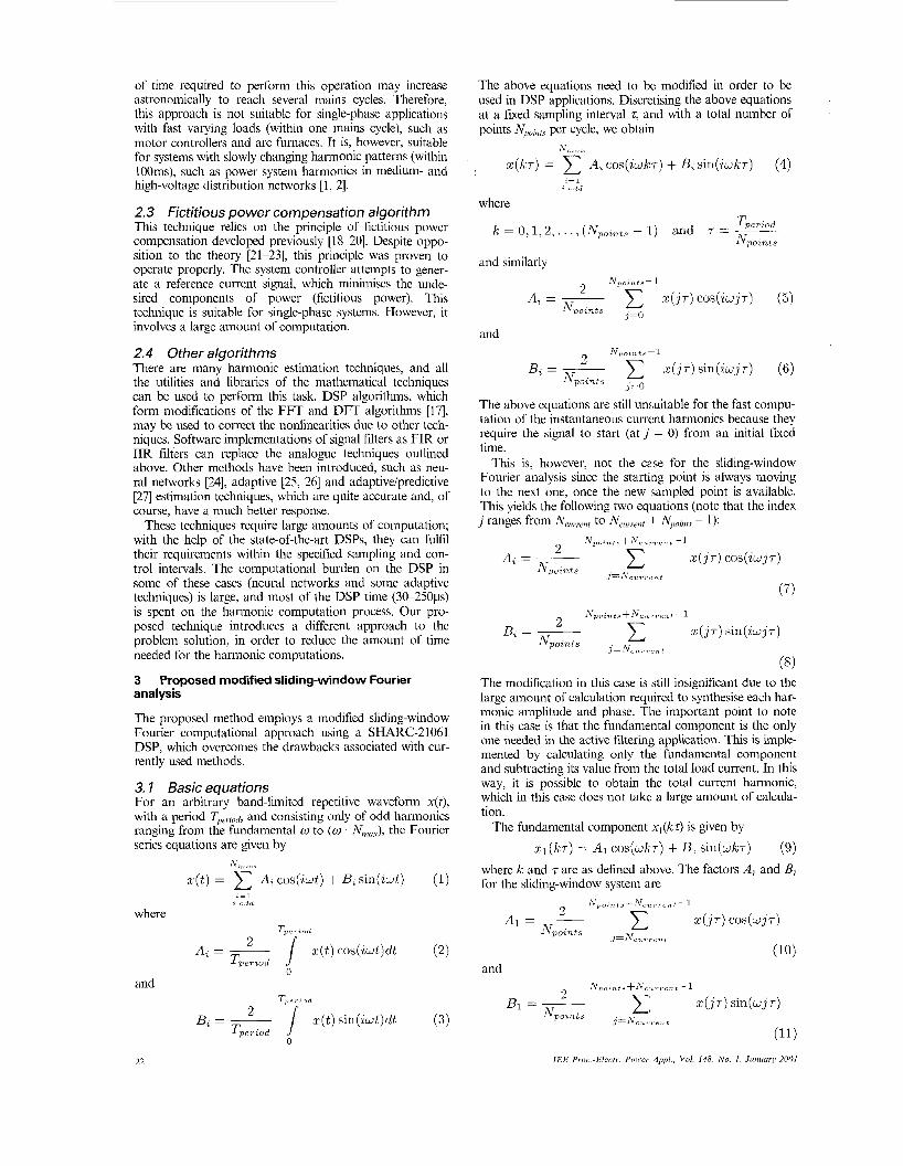
The above equations need to be modified in order to be used in DSP applications. Discretising the above equations at a fixed sampling interval z, arid with a total number of points NPoin, per cycle, we obtain

,=1 2 odd

where

and similarly Np,,t,,t,-l

Z ( j T ) C O S ( 2 W j T ) (5) A . - ~

z -

N p o i n t s j = O

N p o z n t s j z o

and N , m i n t s - - l

B . z - - ___ z(j.r) sin(iwj7) (6)

The above equations are still unsuitable for the fast compu- tation of the instantaneous current harmonics because they require the signal to start (at j = 0) from an initial fixed time.

This is, however, not the case for the sliding-window Fourier analysis since the starting point is always moving to the next one, once the new sampled point is available. This yields the following two equations (note that the index j ranges from NcUrrfnf to Ncu,.,.c',It -+ Npoints - 1):

Np o z 7, t ,* +A', w v r e n t - 1 z A, = - c .(jT) cos(2wj.r)

.I=N,,,, I Npoznts

The modification in this case is still insignificant due to the large amount of calculation required to synthesise each har- monic amplitude and phase. The important point i o note in this case is that the fundamental component is the only one needed in the active filtering application. This is imple- mented by calculating only the fundamental component and subtracting its value from the total Ioad current. In this way, it is possible to obtain the total current harmonic, which in this case does not take a large amount of calcula- tion.

The fundamental component xl(kz) is given by

21 ( k ~ ) = A1 C O S ( W ~ T ) + B1 sin(wk7) (9) where k and z are as defined above. The factors A , and B, for the sliding-window system a re

T,, c I-, " d

22

z ( j 7 ) sin(wj.r) z

B1 = ~

Npoznts 3=n.,t*, 7 c m t

IEE Prm-Elecrr Power App l . , Vol. 148, No. I . Junumy 2001

To obtain the instantaneous values of the desired signal in real time, the values of A , and B, have to be known at that same instant of time. This necessitates the evaluation of the summations in eqns. 10 and 11 at every sampling instant, which is still time consuming.

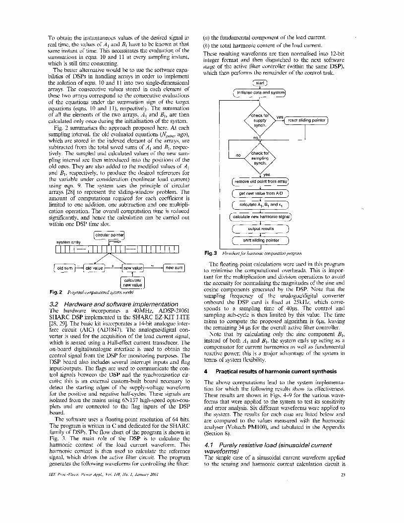
The better alternative would be to use the software capa- bilities of DSPs in handling arrays in order to implement the solution of eqns. 10 and 11 into two single-dimensional arrays. The consecutive values stored in each element of these two arrays correspond to the consecutive evaluations of the equations under the summation sign of the target equations (eqns. 10 and 1 1), respectively. The summation of all the elements of the two arrays, A , and B I , are then calculated only once during the initialisation of the system.

Fig. 2 summarises the approach proposed here. At each sampling interval, the old evaluated equations (N,,,, ago), which are stored in the indexed element of the arrays, are subtracted from the total saved sums of A l and B,, respec- tively. The sampled and calculated values of the new sam- pling interval are then introduced into the positions of the old ones. They are also added to the modified values of A I and B1, respectively, to produce the desired references for the variable under consideration (nonlinear load current) using eqn. 9. The system uses the principle of circular arrays [28] to represent the sliding-window problem. The amount of computations required for each coefficient is limited to one addition, one subtraction and one multipli- cation operation. The overall computation time is reduced significantly, and hence the calculation can be carried out within one DSP time slot.

Fig. 2 Proposed compututiorud system model

3.2 Hardware and software implementation The hardware incorporates a 40MHz, ADSP-2 1061 SHARC DSP implemented in the SHARC EZ-KIT LITE [28, 291. The basic kit incorporates a 14-bit analogue inter- face circuit (AIC) (AD1 847). The analogueidigital con- verter is used for the acquisition of the load current signal, whch is sensed using a Hall-effect current transducer. The on-board digitaUanalogue interface is used to obtain the control signal from the DSP for monitoring purposes. The DSP board also includes several interrupt inputs and flag input/outputs. The flags are used to communicate the con- trol signals between the DSP and the synchronisation cir- cuits; this is an external custom-built board necessary to detect the starting edges of the supply-voltage waveform for the positive and negative half-cycles. These signals are isolated from the mains using 6N137 high-speed opto-cou- plers and are connected to the flag inputs of the DSP board.

The software uses a floating-point resolution of 64 bits. The program is written in C and dedicated for the SHARC family of DSPs. The flow chart of the program is shown in Fig. 3. The main role of the DSP is to calculate the harmonic content of the load current waveform. This harmonic content is then used to calculate the reference signal, which drives the active filter circuit. The program generates the following waveforms for controlling the filter:

IEE P~oc.-Electr. Power Appl , Vol. 148, No. I , .luiiiuiry 2001

(a) the fundamental component of the load current. (b) the total harmonic content of the load current. These resulting waveforms are then normalised into 12-bit integer format and then dispatched to the next software stage of the active filter controller (within the same DSP), which then performs the remainder of the control task.

.I

I A-

synch.

(remove old point from arrad

F===5 get new value from AID +

( calculate A,, B, and x, 1 , L

calculate new harmonic signal 4

( output results I (-) I

The floating-point calculations were used in this program to minimise the computational overheads. This is impor- tant for the multiplication and division operations to avoid the necessity for normalising the magnitudes of the sine and cosine components generated by the DSP. Note that the sampling frequency of the analogueldigital converter onboard the DSP card is fixed at 25kHz, which corre- sponds to a sampling time of 4 0 ~ . The control and sampling sub-cycle is then limited by this value. The time taken to compute the proposed algorithm is 6 p , leaving the remaining 34 ps for the overall active filter controller.

Note that by calculating only the sine component B,, instead of both A, and BI , the system ends up acting as a compensator for current harmonics as well as fundamental reactive power; this is a major advantage of the system in terms of system flexibility.

4 Practical results of harmonic current synthesis

The above computations lead to the system implementa- tion for which the following results show its effectiveness. These results are shown in Figs. 4 9 for the various wave- forms that were applied to the system to test its sensitivity and error analysis. Six different waveforms were applied to the system. The results for each case are listed below and are compared to the values measured with the harmonic analyser (Voltech PMlOO), and tabulated in the Appendix (Section 8).

4.1 Purely resistive load (sinusoidal current waveforms) The simple case of a sinusoidal current waveform applied to the sensing and harmonic current calculation circuit is

23

shown in Fig. 4. Fig. 4a shows the supply voltage wave- form with its phase relation with the load current; in ths case, ths is almost sinusoidal. The hgh-frequency noise on the signal is due to the quantisation error of the oscillo- scope as well as the sampling noise, which accompanies the analogue/digital conversion process. Other sources of noise are due to the fact that the sensing of the sampled current is performed via the Hall-effect transducer which introduces additional noise. The load and supply parame- ters and characteristics are provided in the Appendix (Section 8).

supply voltage in-phase fundamental

CH2 CH 1

load current harmonic component a b

Fig. 4 Pructicul rt,"s of rt$erence current estlnuitorfor pureiy msisrivc loud Voltage scale = 85Vidiv including voltage transducer gain; current scale = 6.25Ndiv including current transducer gain; Zmddiv

Fig. 4a shows a very small phase lag from the current waveform, which is confirmed by the value of 5.9" provided in the Appendix (Section 8). The second wave- form, presented in Fig. 4b, provides the fundamental load current component, which is in phase with the supply volt- age waveform. The harmonics present in the signal are, of course, neghgible, but still exist, as is clear from the corre- sponding table in the Appendix (Section 8).

4.2 Thyristor bridge with resistive load Fig. 5 shows the overall performance of the system under the loading condition of a thyristor bridge feeding a pure resistance. Fig. 5a shows the supply voltage waveform with the load current, which is, of course, a replica of the output voltage waveform. The change of amplitude present in the voltage waveform signal is due to the voltage drop across the supply impedance. This drop is predominant in this case due to the presence of the series current measuring resistance as well as the output impedance of the auto-

transformer used to supply the cmuit. The supply imped- ance is measured to be in the range of 0.8Q

Figs. 5h and c show the fundamental component of the load current as well as its total harmonic content. The difference here is that the first one shows the fundamental component which is in phase with the supply voltage (i.e. compensating for both harmonics and reactive power). The second waveform is the result of 1.he calculation of both A I and B1 in the C program. The magnitudes and phase shfts present in this case show good correspondance with the expected results provided in the Appendix (Section 8).

4.3 Thyristor bridge with resistive/inductive load at minimum triggering angle The most common case of load harmonic spectrum is, of course, the inductive load, which represents most of the industrial loads and conventional DC motor drives. The inductance value used in this case is around 180mH, whch is a reasonably high value as expected in industrial cases. The corresponding current waveform, shown here in Fig. 6a in conjunction with the supply voltage, shows the smoothing effect of the highly inductive load present on the DC side of the thyristor bridge Note that the triggering angle in this case is not exactly zero but is a minimum value of around 13", as provided by the triggering module used in this case. The result wcluld thus be a phase shift between the fundamental component representing only the harmonics (shown in Fig. 6c) arid that incorporating both the harmonics as well as the reactive power compensation (shown in Fig. 6b).

The phase shift of about 18", which is present between the two waveforms, constitutes a reasonable value when compared with the value of 18.3" provided in the corre- sponding table of the Appendix (Section 8) for the h d a - mental component of current. Note also that the non- perfectly flat-topped waveform results in the presence of distortions in each of the two quarter-cycles forming the positive and negative half-cycles. The harmonic compo- nents in the case of Fig. 6b (for which the fundamental current waveform is given to be in phase with the supply voltage) suffer from an unevenness of the positive and neg- ative half-cycles rising and falling edges. This fact is correct for such type of waveforms, which confirms the accuracy of the implemented system.

supply voltage in-phase fundamental complete furidamental

CH 1

CH2 CH2

load current harmonic component harmonic component a b C

Fig. 5 Voltage scale = 85Vidiv including voltage transducer gain; current scale = 6.25Ndiv including current transducer gain; Zmsidiv

Pructicul results of r4erence nrrrrnt estimutor for fJyistor bridge with re.&ive Ioutl

supply voltage in-phase fundamental complete fundamental

load current harmonic component harmonic component a b C

Fig. 6 a = 0; voltage scale = 85Vidiv including voltage transducer gain; current scale = lOA/div including current transducer gain; Zmddiv

24

Pructicul results of refevenee current esfinuiior for thyyistor bridge with inductive loml

I E E Proc.-El~wr. Power Appl. , Vol. 148, No. 1, Jaiiirary 2001

4.4 Thyristor bridge with resistivefinductive load at higher triggering angle Similar to the above loading condition for load parameters and configuration, this case provides a different triggering angle for the load current sensed by the harmonic calcula- tion. For the case of continuous DC side current, the wave- form would simply alter by being phase-shifted, with its magnitude reduced as shown in Fig. 7a. The spikes shown at the transition points are due to the resonance effect between the snubber circuit capacitor connected across the thyristor and the supply inductance. This transient oscilla- tion is due to the energy accompanying the step transition of current path between the two thyristor pairs.

The fundamental harmonic current signal, as shown in Fig. 7c is shown to lag the supply voltage waveform by a value of 59.4", as compared to the value of 58.5" which is shown in the Appendix (Section 8). The thick traces in this case are due to the digitisation noise. Fig. 7b shows the waveform of the fundamental component whch is the result of both the compensation of the harmonics and the reactive power of the load current.

4.5 Thyristor bridge with resistive/capacitive load at minimum triggering angle However uncommon in practice, this load configuration with a thyristor bridge is tested here for the sole purpose of providing the ability to change the wave shape and position of the pulse current, as shown below. This condition of a small triggering angle is similar, to a certain extent, to the case of a diode bridge feeding a rectifier DC-link capacitor, which is very common in AC/DC/AC inverter circuits. This same configuration with a diode bridge is mainly used for

the AC interface of switched mode power supplies. This widespread application (despite the fact that the harmonic pollution accompanying it is of negligible effect due to the extremely small values of currents involved with such sys- tems) constitutes a great danger to the power quality and continuity [7].

The high-amplitude current pulse generated here is shown in Fig. 8a for the load current and supply voltage waveform. As is clearly seen in this case, the supply wave- form is non-sinusoidal. This would not change any of the system performances, except in the case of introducing fur- ther harmonics in the load current; in this case, this would be detected by the harmonic calculation system under investigation. Figs. 8b and c show the harmonic currents and the fundamental components corresponding to the two different cases of harmonic and reactive current compensa- tion as well as harmonic current compensation, respec- tively.

4.6 Thyristor bridge with resistive/capacitive load at higher triggering angle This load configuration is not of any industrial application at all. However, it is presented here for system performance demonstration. The main important characteristic of this waveform is its pulsed current during only a small portion of each half-cycle. The high-amplitude pulse can be shifted from the mid-region of the supply cycle to the right-hand side of the half-cycle. The width of the pulse reduces when shifted to the right at higher triggering angles. This is the main reason why such current waveforms (shown in Fig. 9u) are difficult to compensate. The reference estima- tor has to consider this huge amount of current before the

supply voltage in-phase fundamental complete fundamental

CHI

CH2 CHI

load current harmonic component harmonic component a b C

Fig. 7 Pructicul results of refireme current estunutor jor tliyrktor bridge with inductive loud n > 0; voltage scale = 85V/div including voltage transducer gain; current scale = 10A/div including current transducer gain; 2mddiv

Fig.8 a = 0;1

Pru ioltage

supply voltage in-phase fundamental complete fundamental

current harmonic component harmonic component a b C

cticul results of refmence current estimtor for thyrktor bridge with cupclciiive loud scale = 85Vidiv including voltage transducer gain; current scale = 12A/div including current transducer gain; 2mddiv

CH 1

in-phase fundamental complete fundamental

1

CH2

load current harmonic component harmonic component a b C

Fig. 9 a > 0; voltage scale = X5V/div including voltage transducer gain; current scale = 12Ndiv including current transducer gain; 2mddiv

Pructicul results of reference current esrinzatorfor thyrktor bridge with capacitive loud

I E E Proc.-Electr. Power App l . , Vol. 148, No. I , Junuu~y 2001 25

filter can respond to it. Note that the speed of detection of any variation in this signal is delayed by a few milliseconds since the presence of the zero current periods does not help the calculation process to predict the variation quickly enough.

Similar to the above systems, the fundamental compo- nent in phase with the supply voltage and that correspond- ing to the harmonic elimination are as presented in Figs. 9b and c, respectively. Note that the phase shift of 54.6" for the case of the total fundamental current component corre- sponds to a phase shift of about 54" in the estimated funda- mental signal, which is acceptable under this severe loading condition. The supply voltage in Fig. 9a changes magnitude abruptly at the starting point of the capacitor charging process. This huge drop is because the current rate of rise is very high which interacts with the supply impedance.

5 Static and dynamic response

The proposed reference signal estimator is then used in conjunction with the other system signals to generate the control effort that will drive the PW modulator of the filter switching circuit. It is, however, important to check the sys- tem's static accuracy for the magnitudes and the phase errors.

The calibration of the measuring system can be per- formed taking into account the values measured for the true magnitude of the load fundamental and those calcu- lated by the program. To compare these values, the read- ings must be calibrated and referred to directly directly in amps. This is performed using the case of a purely resistive load in conjunction with a sinusoidal waveform. The meas- ured value of the fundamental component generated by the DSP (generated in volts) (0.8V from Fig. 4b) is used in conjunction with the magnitude measured with the har- monic analyser for the true value of the fundamental load current (from the table in the Appendix (Section 8): 9.35 x cos(-5.9") = 9.3A). If the latter is divided by the former, this results in the constant transformation value of

const = 9.3/0.8 = 11.625 amps/peak volts

This value is then used to generate Table 1 from the data of Figs. 4-9. From this Table, it can be deduced that the percentage error does not exceed 0.925%, which is a good acceptable value for a system static accuracy.

The measurements of the phase angle errors are performed in Table 2. The depicted error values show that the maximum error occurs with a percentage error of 8.47%, which is very high. However, if the absolute error value of 0.5" is considered to be equivalent to a time differ- ence of 27.77p, these small absolute error values can be ignored. The system in this case must then tolerate an error of double the magnitude of the sampling interval, which is in the order of 1.44'. It is obvious from the presented cases

that the system has a maximum value of the error in the order of 0.9", which is well within the tolerance band.

Table 1: Percentage errors in current magnitude measure- ments

% error Measured True value current (A) (A)

Case

1 8.4 8.4 0

2 6.39 6.375 -0.235

3 7.556 7.6 0.579

4 5.81 5.85 0.645

5 14.5 14.4 4 . 9

6 8.425 8.35 -0.925

Table 2 Percentage errors in current phase angle measure- ments

Measured True Absolute phase phase error Case % error

1 5.4" 5.9" -0.4" -8.47%

2 34.2" 34" 0.2" 0.59%

3 18" 18.3" -0.3" -1 64%

4 59.4" 58.5" 0.9" 1.54%

5 4.5" 4.6" -0.1" -2.17%

6 54" 54.6" 4.6" -1.1% ~~

The above error analysis perfixmed for the calculations shows a good performance, which identifies a good accu- racy characteristic for the proposed system. It now remains to analyse the performance of thlz system from the dynamic performance viewpoint. The system in this case whle per- forming a one-cycle integration is expected to have a track- ing error with a maximum of one whole cycle for zero estimation error. However, tb: practical case is much milder.

Consider the proposed system with a fast changing load, as given in Figs. 10 and 11. The various cases outlined show that the performance of the system is rather satisfac- tory and that the error reduces quickly with time. For cases like those in Fig. 10, which have a step change in the load magnitude either increasing (Fig. 10a near zero crossing and Fig. 10b near the peak) or decreasing (Fig. lo(:), this affects the computation process. Note from the curves that the maximum error occurs for a graph like Fig. 106 (where the load current changes near the peak value of the sinusoi- dal waveform). This is the severest case, and a reasonable error value of the order of 10%) can be obtained within less than one half-cycle.

Fig. 11 shows a slowly varying resistive load connected across a rectifying bridge with a reservoir capacitor on the DC side. Part of the resistance is being switched out of the circuit (reducing the load current). The current decay is not

CH1 CHI CH1

CH2 CH2

CH2

a b Fig. 10 CHI = calculated fundamentals; CH2 = actual load current waveform n Decreasing sinusoidal load current near zero crossing; 5Ndiv; 50msidiv b Decreasing sinusoidal load current near peak; SA/div; 20msidiv c Increasing sinusoidal load current near middle cycle; 5Aidiv; 20mddiv

Pructical results of refireme current estimator with dymnic IoLvIilzg conditions C

26 I E E Proc.-Electr. Power Appl. . Vol. 148, No. 1. J n m ~ ~ y 2001

instantaneous. It is, however, sluggish, which gives the esti- mator reasonable time for the calculations to settle down. This mild condition is more expected in the cases of power system applications with slow changes.

CH ’ CHI

aCH2

Fig. 1 1 conditions CHI = SA/div; CH2 = 10Ndiv; 20mddiv a Rectifier bridge with capacitive load current at high triggering angle h Rectifier bridge with capacitive load current at low triggering angle

Pructicul results of refrenee current estiniutor wilh .rynn.lic luding

6 Conclusions

The implementation of the proposed technique on the SHARC processor shows a great deal of flexibility and a major reduction in computation time over ordinary tech- niques using standard FFT and DFT algorithms. It is well suited to the active filter application. If properly imple- mented even on slow and cheap platforms (such as the DSP kit used), it can serve as a fast method for generation of harmonic signals necessary for active power filter opera- tion. The proposed harmonic estimator starts reacting to load changes after a maximum of S o p , which includes the acquisation time (analogue/digital conversion delay) as well as the computation time. The dynamic response of the sys- tem is limited only by the averaging process, which is repre- sented here by the integration necessary for the calculation of the Fourier coefficients. Practical results show that a maximum error of 10% can be reached withm only one half-cycle. The numerous test results show that the system is robust and accurate for a range of test waveforms.

Furthermore, comparing this case with the ordinary slow FFT and DFT algorithms, the proposed system is superior owing to its ability to incorporate a larger number of sam- ples per cycle according to the hardware capabilities of the processor (memory and computational speed) as well as the data acquisition system (analogue/digital acquisition and conversion), without degrading any of the system charac- teristics. A larger number of points can then be used to reduce the effect of noise using numerical manipulation techniques, such as averaging of several consecutive points or oversampling.

References

ARRILAGA, J., BRADLEY, D.A., and BODGER, P.S.: ‘Power sys- tcm harmonics’ (John Wiley and Sons, 1988) AKAGI, H.: ‘New trends in active filters’. Proceedings of Europcan Power Electronics conference, EPE-95, Sevilla, Spain, September 1995, pp. 17-26 GRADY, W.M., SAMOTYJ, M.J., and NOYOLA, A.H.: ‘Survey of active power line conditioning methodologies’, IEEE Trcins. Power Deliv., 1990, 5, (3), pp. 1536-1842 AREDES, M., HAFNER, J., and HEUMANN, K.: ‘Three-phase four-wire shunt active filter control strategies’, IEEE Trans. Power Electron., 1997, 12, (2), pp. 311-318 JOU, H.L.: ‘Performance comparison of the three phase active power filter algorithms’, IEE Proc.-Gener. Transm. Distrib., 1998, 142, (6), pp, 646-682 MEHTA, P., DARWISH, M., and THOMSON, T.: ‘Switched capac- itor filters’, IEEE Trans. Power Electron., 1990, 5, (3), pp. 331-336 KOOZEHKANANI, Z.D., MEHTA, P., and DARWTSH, M.K.: ‘An active filter for retrofit applications’. Proceedings of IEE Power Electronics and Variable Speed Drives, PEVD’96, Nottingham, UK, September 1996, pp. 180-155

IEE Proc-Electr. Power Appl., Vol. 148, No. I , Jununry 2001

8

9

10

11

12

13

14

18

16

17

18

19

20

21

22

23

24

28

26

27

28 29

8

WELSH, M., MEHTA, P., and DARWISH, M.K.: ‘Genetic algo- rithm and extended analysis optimisation techniqucs for switched capacitor active filters - a comparative study’, IEE Proc.-E/ectr. Power Appl., 2000, 147, (I) , pp. 21-26 KOOZEHKANANI, Z.D., MEHTA, P., and DARWISH, M.K.: Active filter for eliminating current harmonics caused by non-linear

circuit elements’, Electron. Lett., 1995, 31, (13), pp. 1041-1042 KOOZEHKANANT, Z.D., MEHTA, P., and DARWISH, M.K.: ‘Active symmetrical lattice filter for harmonic current reduction’. Pro- ceedings of European Power Electronics conference, EPE-98, Sevilla, Spain, September 1995, pp. 869-873 EL-HABROUK, M., DARWISH, M.K., and MEHTA, P.: ‘Analysis and design of a novel active power filter configuration’, IEE Proc.- Electr. Power Appl., 2000, 147, (4), pp. 32Cb328 EL-HABROUK, M.: ‘A new configuration for shunt active filters’. PhD thesis, Department of Electrical Engineering and Electronics, Brunel University, UK, 1998 POULIQUEN, H., LEMERLE, P., and PLANTIVE, E.: ‘Voltage harmonics source compensation using a shunt active filter’. Proceed- ings of European Power Electronics conference, EPE-98, Sevilla, Spain, September 1995, pp. 1.117-1.122 MORAN, L.A., DIXON, J.W., and WALLACE, R.R.: ‘A three phase active power filter operating with fixed switching frequency for reactive power and current harmonic compensation’, IEEE Trcrtis. Ind. Electron., 1995, 42. (4), pp. 402408 KIM, S., PARK, J., KIM, J., CHOE, G., and PARK, M.: ‘An imnroved PWM current control method for harmonic elimination usbg active power filter’. IEEE Industrial Application Society Annual Meeting, IEEE-IAS, 1987, pp. 927-931 CHOE; G., and PARK, M.: ‘Analysis and control of active power fil- ter with optimized injection’, IEEE Trans. P o i i ~ Electron., 1989, 4, (4), pp. 427433 PROAKIS, J.G., and MANOLAKIS, D.G.: ‘Digital signal process- ing: Principles, algorithms and applications’ (Prentice Hall, 1996) ENSLIN, J., and VAN WYK, J.D.: ‘Measurement and compensation of fictitious power under nonsinusoidal voltage and current condi- tions’, IEEE Tvuns. Insrrum. Meus., 1988, 37, (3), pp. 403-408 ENSLIN, J., and VAN WYK, J.D.: ‘A new control philosophy for power electronic converters as fictitious power compensators’, IEEE Trcms. Poii~er Electron., 1990, 5, (I), pp. 88-97 VAN HARMELEN, G.L., and ENSLIN, J.: ‘Real time dynamic con- trol of dynamic power filters in supplies with high contamination’, IEEE Trrrns. Power Electron., 1993, 8, (3), pp. 301-308 FILIPSKI, P.S.: ‘Comments on ‘Measurement and compensation of fictitious power under nonsinusoidal voltage and current conditions”, IEEE Trans. Instrum. Mecis., 1989, 38, (3) CZARNECKI, L.S.: ‘Comments on ‘Measurement and compensation of fictitious power under nonsinusoidal voltage and current condi- tions”, IEEE Truns. Instrum. Meus., 1989, 38, (3) CZARNECKI, L.S.: ‘Comments on ‘A new control philosophy for power electronic converters as fictitious power compensators”, IEEE Truns. Power Electron., 1990, 5, (4) L1, X., and MA, H.: ‘A hybrid estimation model of artificial neural network and weighted least square for harmonic sources identifica- tion’. Proceedings of 7th intemational conference on Htrrmonics cind yuulity qfpoiver, Las Vegas, USA, 1996, Vol. 7, pp. 286-292 LIU, S.: ‘An adaptive Kalman filter for dynamic estimation of har- monic signals’. Proceedings of 8th intemational conference on Hur- nzowics cind yuuliry ofpoiver, Athens, Greece, 1998, pp. 6 3 M 0 LUO, S., and HOU, Z.: ‘An adaptive detecting method for hafmonic and reactive currents’, IEEE Trcins. Ind. Elecrron., 1998, 42, (I), pp. 85-89 VALIVIITA, S., and OVASKA, S.: ‘Delayless method to generate current reference for active filters’. IEEE Truns. Ind. Electron.. 1998. 45, (4), pp. 859-567 ‘ADSP-2 1000 farmly - application handbook’ Analog Devices, 1994 ‘ADSP-2106x SHARC-EZ-KIT Lite, reference manual’ Analog Devices, May 1997

Appendix

The supply parameters (including current measuring devices and auto-transformers) are given as follows:

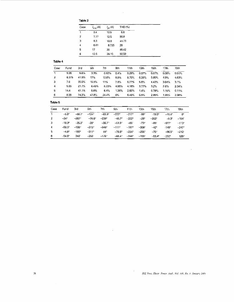
RSouTCe = 0.58 R LsouTce = 1.735 mH The measured load currents of the six loading conditions outlined in the paper are presented in Table 3, with the THD of each case measured using the harmonic analyser (Voltech PMIOO).

The current harmonics measured (A) from the harmonic analyser are given in Table 4.

The phase angles of the each of the harmonics measured from the harmonic analyser for the six cases are given in Table 5.

27

Table 3

Case lrms (A) Ipk (A) THD (YO)

1 9.4 12.5 6.6

2 7.17 12.5 50.8

3 8.3 10.9 44.73

4 6.01 8.725 26

5 17 30 48.42

6 12.5 28.15 92.59

Table 4

Case Fund 3rd 5th 7th 9th 11th 13th 15th 17th 19th

1 9.35 5.6% 3.3% 0.82% 0.4% 0.29% 0.07% 0.07% 0.089; 0.01%

2 6.375 41.9% 17% 12.6% 8.9% 8.75% 6.26% 5.95% 4.9% 4.63%

3 7.6 35.5% 19.5% 11% 7.8% 6.77% 5.6% 4.43% 3.64Yo 3.1%

4 5.85 21.7% 6.45% 6.23% 4.95% 4.18% 3.77% 3.2% 2.8% 2.34%

5 14.4 47.1% 5.8% 8.4% 1.36% 2.65% 1.4% 0.79% 1.15% 0.11%

6 8.35 74.3% 47.8% 24.4% 6% 6.46% 6.5% 2.95% 1.95% 2.96%

Table 5

Case Fund 3rd 5th 7th 9th 11th 13th 15th 17th 19th

1 -5.9" 66.7" -124" -83.3" -222" -217' -99" -19.5" -ltL4° 0"

2 -34" -262" -75.6" -238" -45.7" -222" -28" -202" -0.3" -184"

3 -18.3" -25.3' -29" -36.7" -51.9" -65" -73" -85" -97'1" -113"

4 58.5" -106" -273" -346" -111" -197" -308" -42" -14!3" -247"

5 -4.6" -180" -311" 44" -76.8" -234" -256" -70" -86.5" -212"

6 -54.6" 340" -259" -176" -68.4" -248' -155" -53.4" -23:2" -125"

28 IEE Proc -Elecrr. Power. Appl.. Vol. 148, No. 1 . Junuury 2001