Design and Implementation of a Novel Dataﬂow Model and an ...

Design and Implementation of a Novel Dataflow Model and anIntermediate Representation Language for High Level Synthesis

on Field Programmable Gate Arrays

Jeppe Græsdal Johansen

December 3, 2012

Electronic Systems, ASPIInstitute 8Fredrik Bajers Vej 7 A19220 Aalborg Øhttp://es.aau.dk/

Title:Design and Implementation of a NovelDataflow Model and an Intermediate Rep-resentation Language for High Level Syn-thesis on Field Programmable Gate Arrays

Project period:10th semester, 2012

Project group:12gr1042

Participant:Jeppe Græsdal Johansen

Number of copies: 5

Number of pages: 52

Appendices: CD-ROM

Finished 3rd of December 2012

Abstract:

FPGAs are large matrices of logic blocks which op-erate concurrently. Their design allow massive par-allel processing of data, but the limiting factor isoften the tools and design methodologies used toprogram them with.Many different languages exists that try to solve thisproblem, but not many enjoy widespread use dueto limitations in either the level of abstraction theyoffer, or limitations in what performance they candeliver compared to traditional low-level designs.The report looks at a few of such high level lan-guages, and the design of an early supercomputerarchitecture is investigated. The report proposes anew dataflow model which adopt the good featuresof all of those. A high-level intermediate represen-tation language is designed to effectively expressthe dataflow in this proposed dataflow model. Fur-ther, a number of heuristics are proposed which aredesigned to facilitate optimization of the generatedFPGA design.The result is a dataflow model which is remarkablein its simplicity, and is tailored well for expressingcomplex digital signal processing algorithms.A comparison between another high-level synthe-sis language shows that the overall execution speedperformance is slightly lower. However, the area re-quired was comparable to other solutions. The moreflexible dataflow model increases transport over-head, but it greatly increases the expressive powerof the model.

3

http://es.aau.dk/

Preface

This report documents the work done by group 12gr1042 during their project on the 4th semester project of themaster with specialization in Applied Signal Processing and Implementation at Aalborg University and is titled:Design and Implementation of a Novel Dataflow Model and an Intermediate Representation Language for HighLevel Synthesis on Field Programmable Gate Arrays.

The report is organized into 6 parts:

Introduction This section investigates FPGAs, and the challenges in designing programs for them. A number ofprevious solutions are investigated.

Analysis Based on the technologies investigated in the introduction, a new design for a dataflow model, an inter-mediate representation language, and a set of heuristics are proposed to solve the issues of designing FPGAsystems.

Specification This section describes the syntax of the proposed language.

Implementation The implementation of a compiler which can compile the intermediate representation into Ver-ilog HDL code is described.

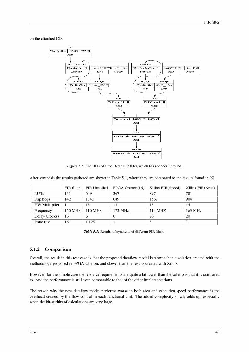
Test A testcase is performed, where a program is compiled and synthesized, and the resulting FPGA program iscompared to previous implementations of it in another high-level synthesis language.

Conclusion The project is concluded, the results of the project are discussed, and potential subjects for futurework is discussed.

The CD contains the source code for the compiler implementation, and example code.

Jeppe Græsdal Johansen

Contents

Preface . . . . . . . . . . . . . . . . . . . . . . . . . . . . . . . . . . . . . . . . . . . . . . . . . . . .

I Report 1

1 Introduction 31.1 FPGAs . . . . . . . . . . . . . . . . . . . . . . . . . . . . . . . . . . . . . . . . . . . . . . . . . 31.2 FPGA programming . . . . . . . . . . . . . . . . . . . . . . . . . . . . . . . . . . . . . . . . . 4

1.2.1 FPGA-Oberon . . . . . . . . . . . . . . . . . . . . . . . . . . . . . . . . . . . . . . . . 51.2.2 CAL . . . . . . . . . . . . . . . . . . . . . . . . . . . . . . . . . . . . . . . . . . . . . 51.2.3 Vivado HLS . . . . . . . . . . . . . . . . . . . . . . . . . . . . . . . . . . . . . . . . . . 6

1.3 Decoupled Access/Execute Architectures . . . . . . . . . . . . . . . . . . . . . . . . . . . . . . 6

2 Analysis 92.1 Problem definition . . . . . . . . . . . . . . . . . . . . . . . . . . . . . . . . . . . . . . . . . . 92.2 Problem scope . . . . . . . . . . . . . . . . . . . . . . . . . . . . . . . . . . . . . . . . . . . . . 92.3 Proposed methodology . . . . . . . . . . . . . . . . . . . . . . . . . . . . . . . . . . . . . . . . 92.4 Dataflow model . . . . . . . . . . . . . . . . . . . . . . . . . . . . . . . . . . . . . . . . . . . . 9

2.4.1 Design objective . . . . . . . . . . . . . . . . . . . . . . . . . . . . . . . . . . . . . . . 92.4.2 Datapath with coarse-grained synchronization . . . . . . . . . . . . . . . . . . . . . . . . 102.4.3 Datapath with fine-grained synchronization . . . . . . . . . . . . . . . . . . . . . . . . . 102.4.4 Memory access . . . . . . . . . . . . . . . . . . . . . . . . . . . . . . . . . . . . . . . . 11

2.5 Functional units primitives . . . . . . . . . . . . . . . . . . . . . . . . . . . . . . . . . . . . . . 112.5.1 Constants . . . . . . . . . . . . . . . . . . . . . . . . . . . . . . . . . . . . . . . . . . . 112.5.2 Arithmetic operations . . . . . . . . . . . . . . . . . . . . . . . . . . . . . . . . . . . . . 122.5.3 Memory blocks and load/store units . . . . . . . . . . . . . . . . . . . . . . . . . . . . . 132.5.4 Maintaining synchronicity . . . . . . . . . . . . . . . . . . . . . . . . . . . . . . . . . . 132.5.5 Memory units . . . . . . . . . . . . . . . . . . . . . . . . . . . . . . . . . . . . . . . . . 142.5.6 Accumulator units . . . . . . . . . . . . . . . . . . . . . . . . . . . . . . . . . . . . . . 14

2.6 Language structure . . . . . . . . . . . . . . . . . . . . . . . . . . . . . . . . . . . . . . . . . . 142.6.1 Values . . . . . . . . . . . . . . . . . . . . . . . . . . . . . . . . . . . . . . . . . . . . . 152.6.2 Operations . . . . . . . . . . . . . . . . . . . . . . . . . . . . . . . . . . . . . . . . . . 152.6.3 Assignments . . . . . . . . . . . . . . . . . . . . . . . . . . . . . . . . . . . . . . . . . 152.6.4 Function calls . . . . . . . . . . . . . . . . . . . . . . . . . . . . . . . . . . . . . . . . . 152.6.5 Control structures . . . . . . . . . . . . . . . . . . . . . . . . . . . . . . . . . . . . . . . 162.6.6 Data types . . . . . . . . . . . . . . . . . . . . . . . . . . . . . . . . . . . . . . . . . . . 162.6.7 Memory allocation . . . . . . . . . . . . . . . . . . . . . . . . . . . . . . . . . . . . . . 18

2.7 Compilation process . . . . . . . . . . . . . . . . . . . . . . . . . . . . . . . . . . . . . . . . . 182.7.1 IR processing . . . . . . . . . . . . . . . . . . . . . . . . . . . . . . . . . . . . . . . . . 20

2.8 Heuristics . . . . . . . . . . . . . . . . . . . . . . . . . . . . . . . . . . . . . . . . . . . . . . . 202.8.1 Loop body heuristics . . . . . . . . . . . . . . . . . . . . . . . . . . . . . . . . . . . . . 202.8.2 Loop transformations . . . . . . . . . . . . . . . . . . . . . . . . . . . . . . . . . . . . . 22

CONTENTS

3 Specification 253.1 Synthesizable operations . . . . . . . . . . . . . . . . . . . . . . . . . . . . . . . . . . . . . . . 253.2 Helper operations . . . . . . . . . . . . . . . . . . . . . . . . . . . . . . . . . . . . . . . . . . . 273.3 Floating point operations . . . . . . . . . . . . . . . . . . . . . . . . . . . . . . . . . . . . . . . 28

4 Implementation 314.1 Compiler . . . . . . . . . . . . . . . . . . . . . . . . . . . . . . . . . . . . . . . . . . . . . . . 31

4.1.1 Structure . . . . . . . . . . . . . . . . . . . . . . . . . . . . . . . . . . . . . . . . . . . 314.1.2 Scanner and parser . . . . . . . . . . . . . . . . . . . . . . . . . . . . . . . . . . . . . . 314.1.3 Constant propagation . . . . . . . . . . . . . . . . . . . . . . . . . . . . . . . . . . . . . 324.1.4 Operation simplification . . . . . . . . . . . . . . . . . . . . . . . . . . . . . . . . . . . 324.1.5 Unused code removal . . . . . . . . . . . . . . . . . . . . . . . . . . . . . . . . . . . . . 324.1.6 Loop counter insertion . . . . . . . . . . . . . . . . . . . . . . . . . . . . . . . . . . . . 334.1.7 Bit-width analysis . . . . . . . . . . . . . . . . . . . . . . . . . . . . . . . . . . . . . . 354.1.8 Verilog code generation . . . . . . . . . . . . . . . . . . . . . . . . . . . . . . . . . . . 35

5 Test 415.1 FIR filter . . . . . . . . . . . . . . . . . . . . . . . . . . . . . . . . . . . . . . . . . . . . . . . . 41

5.1.1 Compilation . . . . . . . . . . . . . . . . . . . . . . . . . . . . . . . . . . . . . . . . . 425.1.2 Comparison . . . . . . . . . . . . . . . . . . . . . . . . . . . . . . . . . . . . . . . . . . 43

6 Conclusion 456.1 Conclusion . . . . . . . . . . . . . . . . . . . . . . . . . . . . . . . . . . . . . . . . . . . . . . 456.2 Discussion . . . . . . . . . . . . . . . . . . . . . . . . . . . . . . . . . . . . . . . . . . . . . . . 456.3 Future work . . . . . . . . . . . . . . . . . . . . . . . . . . . . . . . . . . . . . . . . . . . . . . 46

II Appendix 49

A Appendix 51A.1 IR Syntax . . . . . . . . . . . . . . . . . . . . . . . . . . . . . . . . . . . . . . . . . . . . . . . 51

CONTENTS

Part I

Report

1Introduction

1.1 FPGAs

In different places in electronics there will always be a need to process huge amounts of data in a short time. Tech-nologies such as video compression, wireless communication, and computer vision are examples of computingdomains where massive amounts of data needs to be processed in realtime. For a long time in the history of inte-grated circuits, the only option for system designers was to design an ASIC (application specific integrated circuit)from scratch and put it in mass production. Designing a chip from scratch was an expensive and time consumingprocess, and problems in the chip after manufacture were hard to fix.

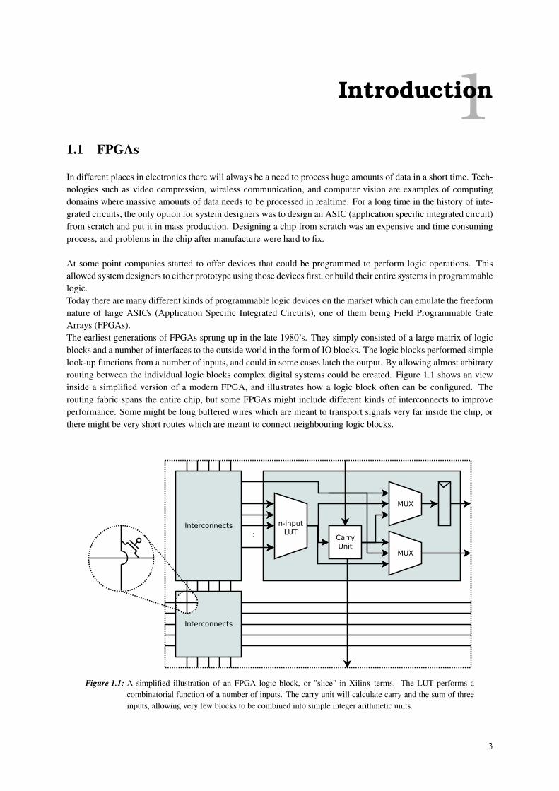
At some point companies started to offer devices that could be programmed to perform logic operations. Thisallowed system designers to either prototype using those devices first, or build their entire systems in programmablelogic.Today there are many different kinds of programmable logic devices on the market which can emulate the freeformnature of large ASICs (Application Specific Integrated Circuits), one of them being Field Programmable GateArrays (FPGAs).The earliest generations of FPGAs sprung up in the late 1980’s. They simply consisted of a large matrix of logicblocks and a number of interfaces to the outside world in the form of IO blocks. The logic blocks performed simplelook-up functions from a number of inputs, and could in some cases latch the output. By allowing almost arbitraryrouting between the individual logic blocks complex digital systems could be created. Figure 1.1 shows an viewinside a simplified version of a modern FPGA, and illustrates how a logic block often can be configured. Therouting fabric spans the entire chip, but some FPGAs might include different kinds of interconnects to improveperformance. Some might be long buffered wires which are meant to transport signals very far inside the chip, orthere might be very short routes which are meant to connect neighbouring logic blocks.

Interconnects

: CarryUnit

Interconnects n-inputLUT

MUX

MUX

Figure 1.1: A simplified illustration of an FPGA logic block, or "slice" in Xilinx terms. The LUT performs acombinatorial function of a number of inputs. The carry unit will calculate carry and the sum of threeinputs, allowing very few blocks to be combined into simple integer arithmetic units.

3

FPGA programming

The basic structure of FPGAs has largely stayed the same, but in the last few generations chip designers havestarted to integrate more complex features, such as hardware multipliers, embedded RAM (Random Access Mem-ory), advanced clock synthesis units, and more advanced IO signaling options. Those options are winning largeracceptance due to the rising need of integrating a systems complexity on a single chip, that can be required tomaintain high data throughput, and operating frequency. Utilizing those resources effectively is instrumental inextracting the power of the FPGA design.

1.2 FPGA programming

Designing firmware for FPGAs is different from designing software for a traditional general purpose processor(GPP). In a GPP system, a programmer can mostly assume that the processor executes a stream of simple instruc-tions in a sequential order; however, on an FPGA there is no such concept as instructions. The FPGA fabric needsto be programmed to do something first, and all the logic has to be interconnected to make sense. Creating thisarchitecture has been, and still is, a very complicated task.

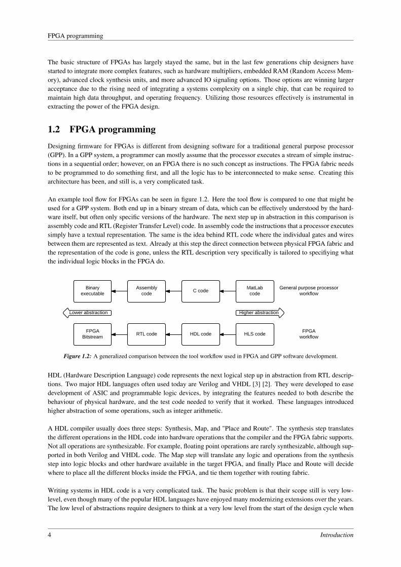
An example tool flow for FPGAs can be seen in figure 1.2. Here the tool flow is compared to one that might beused for a GPP system. Both end up in a binary stream of data, which can be effectively understood by the hard-ware itself, but often only specific versions of the hardware. The next step up in abstraction in this comparison isassembly code and RTL (Register Transfer Level) code. In assembly code the instructions that a processor executessimply have a textual representation. The same is the idea behind RTL code where the individual gates and wiresbetween them are represented as text. Already at this step the direct connection between physical FPGA fabric andthe representation of the code is gone, unless the RTL description very specifically is tailored to specifiying whatthe individual logic blocks in the FPGA do.

Figure 1.2: A generalized comparison between the tool workflow used in FPGA and GPP software development.

HDL (Hardware Description Language) code represents the next logical step up in abstraction from RTL descrip-tions. Two major HDL languages often used today are Verilog and VHDL [3] [2]. They were developed to easedevelopment of ASIC and programmable logic devices, by integrating the features needed to both describe thebehaviour of physical hardware, and the test code needed to verify that it worked. These languages introducedhigher abstraction of some operations, such as integer arithmetic.

A HDL compiler usually does three steps: Synthesis, Map, and "Place and Route". The synthesis step translatesthe different operations in the HDL code into hardware operations that the compiler and the FPGA fabric supports.Not all operations are synthesizable. For example, floating point operations are rarely synthesizable, although sup-ported in both Verilog and VHDL code. The Map step will translate any logic and operations from the synthesisstep into logic blocks and other hardware available in the target FPGA, and finally Place and Route will decidewhere to place all the different blocks inside the FPGA, and tie them together with routing fabric.

Writing systems in HDL code is a very complicated task. The basic problem is that their scope still is very low-level, even though many of the popular HDL languages have enjoyed many modernizing extensions over the years.The low level of abstractions require designers to think at a very low level from the start of the design cycle when

4 Introduction

FPGA programming

assigning functionality to different sub-modules of a design.Many have tried to develop languages that give a higher abstraction of the hardware, but not many have won broadacceptance as being an acceptable tool as a replacement for traditional HDL design. These classes of languages,which tries to raise the abstraction level, are often referred to as High-Level Synthesis (HLS) languages or HLStools.

1.2.1 FPGA-Oberon

FPGA-Oberon was a HLS language which was designed to solve the problem of designing complex systems fordigital signal processing on FPGAs [5]. The basic idea behind the language was to entirely remove the conceptof the underlying FPGA architecture from the language, and instead use high-level vector processing syntax con-structs to allow the compiler to construct a single stream-oriented FPGA RTL description. In particular the reportargued that the basic construction of the FPGA hardware suited constructions of large pipelined datapaths betterthan register based time-sharing statemachines with simple datapaths (ASMDs).

The data flow model proposed in the report is very simple, in the sense that every calculation in an FPGA-Oberonprogram has its own functional unit. This effectively solve the scheduling problem which is a a problem in resourceconstrained ASMDs, since no functional units are shared with other intermediate calculations. The justificationused for this data flow model is that selection logic, such as multiplexers, is expensive in the number of logicblocks it requires, and that it puts strain on the fan-out of the functional units that it has as inputs. In a logicblock approximation model proposed in the report it was found that their cost was a function of both the outputbitwidth and the number of inputs. It was found that most integer operations only was a linear function of theoutput bitwidth.It was concluded that the method showed great promise in solving some of the basic problems around designingDSP systems for FPGAs, but a number of issues were left which limited its usefulness in many realworld cases.

Two of the biggest issues were the lack of dynamic or more complex memory access, and the synchronizationbetween functional units in the datapath. There was not any real functionality developed that could handle local orglobal congestation in the datapath.

1.2.2 CAL

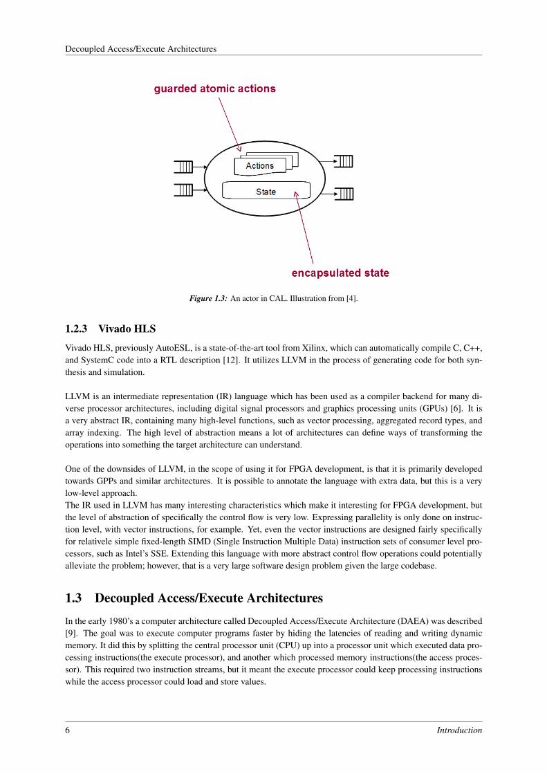
Another language slightly similar to FPGA-Oberon is Caltrop Actor Language (CAL)t [1]. CAL is an actorlanguage which can be used to describe actors and how they interac. An actor can be seen as a module whichoperate and communicate concurrently with other actors. In this sense it models the fabric of an FPGA quite wellin that every logic block operates concurrently. It was shown that actors, and CAL specifically, can be used as aHLS tool to develop complex FPGA programs [4]. One of the reasons why it has many advantages over normalHDL programming is that it is defined at a higher abstraction level which removes some of the need to think abouthow submodules of a design communicate. Interconnects between actors are simple FIFO queues, references aschannels. Figure 1.3 shows an actor, which is comprised of an internal state, a number of input and output channels,and a set of actions.Actions perform operations on any input data and the state, and are triggered by certain conditions, such as externalstimulus.

Using a channel oriented design allows a more relaxed design process to take place since there are no requirementsabout the arrival times of any required inputs, which makes designcycles easier; however, the abstraction level isonly slightly above RTL since the actions in the actors themselves are denoted as simple processes. There is somesupport for higher level control flow and datatypes, such as for loops and lists, although they are only defined on abehavioural level. There is no specification for how it should be mapped to hardware.The dataflow model used in FPGA-Oberon can be compared to a subset of the model used in CAL, except FPGA-Oberon did not have a sufficiently advanced channel concept.

Introduction 5

Decoupled Access/Execute Architectures

Figure 1.3: An actor in CAL. Illustration from [4].

1.2.3 Vivado HLS

Vivado HLS, previously AutoESL, is a state-of-the-art tool from Xilinx, which can automatically compile C, C++,and SystemC code into a RTL description [12]. It utilizes LLVM in the process of generating code for both syn-thesis and simulation.

LLVM is an intermediate representation (IR) language which has been used as a compiler backend for many di-verse processor architectures, including digital signal processors and graphics processing units (GPUs) [6]. It isa very abstract IR, containing many high-level functions, such as vector processing, aggregated record types, andarray indexing. The high level of abstraction means a lot of architectures can define ways of transforming theoperations into something the target architecture can understand.

One of the downsides of LLVM, in the scope of using it for FPGA development, is that it is primarily developedtowards GPPs and similar architectures. It is possible to annotate the language with extra data, but this is a verylow-level approach.The IR used in LLVM has many interesting characteristics which make it interesting for FPGA development, butthe level of abstraction of specifically the control flow is very low. Expressing parallelity is only done on instruc-tion level, with vector instructions, for example. Yet, even the vector instructions are designed fairly specificallyfor relativele simple fixed-length SIMD (Single Instruction Multiple Data) instruction sets of consumer level pro-cessors, such as Intel’s SSE. Extending this language with more abstract control flow operations could potentiallyalleviate the problem; however, that is a very large software design problem given the large codebase.

1.3 Decoupled Access/Execute Architectures

In the early 1980’s a computer architecture called Decoupled Access/Execute Architecture (DAEA) was described[9]. The goal was to execute computer programs faster by hiding the latencies of reading and writing dynamicmemory. It did this by splitting the central processor unit (CPU) up into a processor unit which executed data pro-cessing instructions(the execute processor), and another which processed memory instructions(the access proces-sor). This required two instruction streams, but it meant the execute processor could keep processing instructionswhile the access processor could load and store values.

6 Introduction


Figure 1.4: A block diagram of a decoupled access/execute architecture. The execute processor is denoted as EP,and the access processor is the AP. Illustration from [8].

Figure 1.4 shows an example of a DAEA system. The two processors communicate using queues. Whenever aprogram needs to load a value from RAM, the access processor would execute a load instruction. The address isgenerated sent to the memory controller, which will push a value back into a load queue when done.When the execute processor actually needs the loaded value it can wait for it in the load queue. In a naive imple-mentation of such architecture, neither of the processors do not have to wait for stores to finish, so the memorycontroller can simply store a value when both an address and a value is ready in their respective queues.

This decoupling of memory and data operations was a simple way to improve performance in early supercomputers.It later lost recognition as an effective technique due to much more advanced superscalar processor architecturesbeing developed which performed much better with a simpler design for the programmer. Despite the simplicityof the hardware concept of DAEA it puts many requirements on the code itself. Load and store requests have to bedone in the correct order, and stalling due to dynamic memory latencies can be hard to predict. Further, this systemmade it hard to use processor interrupts, which is often required by preemptive multitasking, due to the processornot being able to know whether a load or a store is in progress.

While the architecture enjoys no large use anymore in mainstream processors, it is very interesting in the scopeof FPGAs. The techniques used to implement dynamic memory latency hiding in modern processors rely onvery complicated algorithms, such as the Tomasulo algorithm, and scoreboarding [8]. These techniques onlyhave limited use in FPGAs since they take up a lot of memory and logic blocks, and only apply to architecturesresembling normal GPPs, which despite their flexibility are not very efficient in FPGA fabric.

Introduction 7


8 Introduction

2Analysis

2.1 Problem definition

As explained in the introduction, the task of designing firmware for FPGAs is a complicated process. The designtools often used are either too low-level in abstraction, or not very good at expressing parallelity.A number of existing solutions for this problem, and a processor architecture was investigated, and some of theiradvantages or interesting properties were examined.

This leads to the following problem specification:

Can a higher level of abstraction of a simple IR language, combined with a datapath orienteddataflow model be used to facilitate FPGA design, by allowing the compiler to simply apply heuristicfunctions to find out how to transform it into an efficient FPGA architecture? Further, can decoupledaccess/execute architectures solve the design problems of datapaths with high memory addressingcomplexity or contention?

2.2 Problem scope

The scope of this project is mainly to investigate dataflow models and control flow constructs, and developingmapping heuristics tailored towards dataflow intensive programs, such as DSP algorithms.

Further, a goal of this project is to develop a simple programming language that can be interfaced as a link betweenexisting programming languages and a compiler which can generate FPGA programs.

2.3 Proposed methodology

This project proposes a new dataflow model which derives the basic dataflow concept from the methodologyproposed in FPGA-Oberon, and extends it with simpler and more versatile synchronization inspired by the channelconcept of CAL, and random memory access primitives inspired by the concept behind decoupled access/executearchitectures. Further, it proposes a high-level Intermediate Representation (IR) language which can describe suchsystems. This language is inspired by LLVM, and resembles existing 3-address code languages, but with high-level flow control syntax, and will be shown to be beneficial as an intermediate step because of the FPGA specifictransformations it allows.

2.4 Dataflow model

2.4.1 Design objective

Designing a new dataflow model should attempt to accomodate a number of common goals:

1. High possible operating frequency.

2. High data throughput.

3. Low power consumption.

4. Low area requirement.

9

Dataflow model

2.4.2 Datapath with coarse-grained synchronization

A dataflow model, as used in [5], put no special consideration into dynamic memory access latencies, hence itwas very cumbersome to design large systems with. This put a constraint on what memory configurations werepossible, and in turn limited the type of algorithms the method could be used to implement.

Further, due to the synchronization mechanism choosen any local contention would stall the rest of the preceedingdatapath until the required results were finished. This could be solved for simple systems by mapping the algorithmin a way that it would never create congestation, but for arbitrarily large systems this became a very complicatedissue to fix.

2.4.3 Datapath with fine-grained synchronization

Instead this project proposes a different dataflow model: A simpler method for designing datapaths, than those in-vestigated, would be to create a fine-grained handshake structure for every functional unit in the design. A minimalversion of this handshake structure is shown in Figure 2.1.

All operations in a design, using this method, operate synchronously, and are assumed to be connected to the sameclock network. Input or output ports are not required to be connected to any other port, but unconnected ports willbe signalled as having either no data ready, or being always busy.

Table 2.1 specify which actions must be taken for each clock cycle of an output port, and any connected inputports. If more than one input port is connected to an output port all input ports must signal DataBusy = 0 beforeany action can happen, as indicated with !0.

DataReady DataBusy Action0 0 No action1 0 Transfer data0 not 0 No action1 not 0 Stall output port, and signal busy to any in-

put ports of the unit.

Table 2.1: This table shows the actions performed by an output port, and one or more input ports.

Input Port

Data

DataReady

DataBusy

Output Port

Data

DataReady

DataBusy Functional unit

Inputport 0

Inputport n-1

Outputport 0

Outputport n-1

Figure 2.1: This sketch shows the input and output ports of a functional unit.

The area requirements for the logic to handle this form of handshaking is very low, since the protocol is as simpleas it is. This design could further facilitate the low power objective, since functional units only has to do workwhen new data is presented.

10 Analysis

Functional units primitives

2.4.4 Memory access

Explicit use of random memory access is a feature seldomly required in DSP algorithms. Yet, in very complexalgorithms storage of intermediate or delayed values can exceed the natural capacity of the logic elements of anFPGA. In this case dedicated RAM blocks are required, which introduces complicated issues. Figure 2.2 showsthe different RAM configurations in an FPGA.

The advantages of LUT-based RAM is that all elements can be accessed at the same time in a single clock cycle.This gives an enormous possible throughput. But the flexibility is low since dynamically indexing the RAM wouldrequire much extra logic, which at the same time would slow the overall design down.

Block RAM are small blocks of dedicated RAM that are physically spread around inside the FPGA. These blocksare usually designed as dual-port RAM, which means users can either read two different addresses, or read andwrite two different addresses in a single clock cycle. These blocks can often be configured in many ways withparameters such as the bit-width of the elements, or the address bus width, but their total capacity is often in thetens of kilo-bits range.

If more capacity is required, a designer might have to integrate an external RAM block in the design. These blockscan have up to giga-bit capacity, but they require complex controllers to function. This project won’t consider thistype of RAM, but the overall methodology could accomodate this type of memory access in the same way as withblock RAM.

Figure 2.2: This comparison shows the relationship between different kinds of implementations of RAM blocks ina Virtex-6 FPGA. Illustration from [7].

Due to the design with fine-grained synchronization, memory access can be performed without regards to whatkind of fabric the memory is stored in. Any dynamic delays will be handled by the synchronization between thefollowing blocks.

2.5 Functional units primitives

To allow most DSP algorithms to be expressed a set of functional unit blocks must be defined to provide a baselinefor the dataflow model. These blocks consists of 6 groups: Constants, arithmetic and bit-wise logic operations,counters, accumulators, memories, and load/store blocks.

2.5.1 Constants

A constant is perhaps the simplest unit. It only has a single output port, which always has data ready and alwayshas the same integer value on the data port.

Analysis 11


2.5.2 Arithmetic operations

Arithmetic operations are binary integer operations. These operations have two input ports, "X", and "Y", and anoutput port called "Result". The operations consists of the following:

Name Description Operationadd Integer addition Result = X +Ysub Integer subtraction Result = X−Ymul Integer multiplication Result = X ∗Yand Bitwise ∧ operation Result = X ∧Yor Bitwise ∨ operation Result = X ∨Yxor Bitwise ⊕ operation Result = X⊕Y

Any unary operations, such as ¬ (bit-wise not), and negation, can be built using the above operations and constants.

The model contains a single ternary operator with the input ports "X", "Y", and "Z", and the output port "Result":

Name Description Operationmac Integer multiply and accumulate Result = X ∗Y +Z

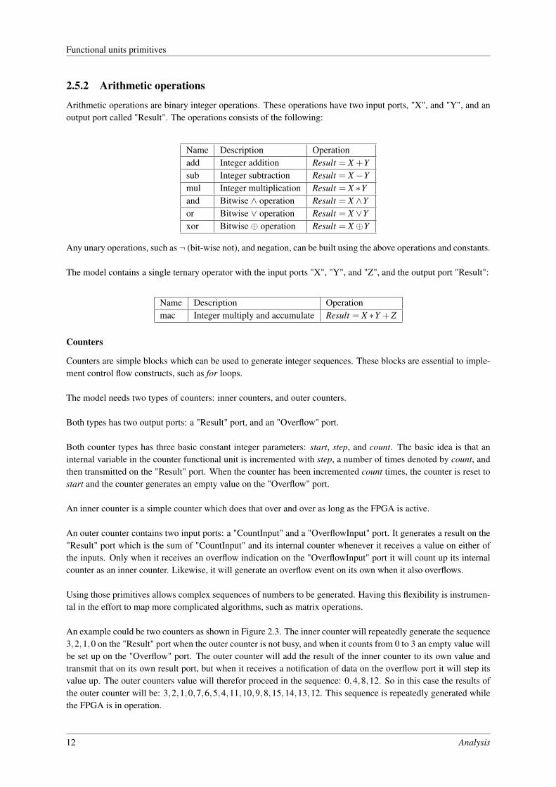
Counters

Counters are simple blocks which can be used to generate integer sequences. These blocks are essential to imple-ment control flow constructs, such as for loops.

The model needs two types of counters: inner counters, and outer counters.

Both types has two output ports: a "Result" port, and an "Overflow" port.

Both counter types has three basic constant integer parameters: start, step, and count. The basic idea is that aninternal variable in the counter functional unit is incremented with step, a number of times denoted by count, andthen transmitted on the "Result" port. When the counter has been incremented count times, the counter is reset tostart and the counter generates an empty value on the "Overflow" port.

An inner counter is a simple counter which does that over and over as long as the FPGA is active.

An outer counter contains two input ports: a "CountInput" and a "OverflowInput" port. It generates a result on the"Result" port which is the sum of "CountInput" and its internal counter whenever it receives a value on either ofthe inputs. Only when it receives an overflow indication on the "OverflowInput" port it will count up its internalcounter as an inner counter. Likewise, it will generate an overflow event on its own when it also overflows.

Using those primitives allows complex sequences of numbers to be generated. Having this flexibility is instrumen-tal in the effort to map more complicated algorithms, such as matrix operations.

An example could be two counters as shown in Figure 2.3. The inner counter will repeatedly generate the sequence3,2,1,0 on the "Result" port when the outer counter is not busy, and when it counts from 0 to 3 an empty value willbe set up on the "Overflow" port. The outer counter will add the result of the inner counter to its own value andtransmit that on its own result port, but when it receives a notification of data on the overflow port it will step itsvalue up. The outer counters value will therefor proceed in the sequence: 0,4,8,12. So in this case the results ofthe outer counter will be: 3,2,1,0,7,6,5,4,11,10,9,8,15,14,13,12. This sequence is repeatedly generated whilethe FPGA is in operation.

12 Analysis


Inner counterStart: 3Step: -1Count: 4

Result

Overflow

Outer counterStart: 0Step: 4

Count: 4

Result

Overflow

CountInput

OverflowInput

Figure 2.3: Two counters connected to generate a complex sequence of integers. In this case the sequence is 16elements long: 3,2,1,0,7,6,5,4,11,10,9,8,15,14,13,12

2.5.3 Memory blocks and load/store units

This model will include three types of memory primitives: a delayline unit, a constant RAM unit, and a RAM unit.To access those there are two types of blocks: a load unit and a store unit.

A load unit is connected to a memory primitive with two ports: an "AddrOut" port and a "ValueIn" port. Storeunits use two output ports: an "AddrOut" and a "ValueOut" port. This concept is illustrated in Figure 2.4.

For load units the idea is that whenever it receives an address on its "AddrIn" port it will forward this to the memoryunit. When the memory unit is ready and has fetched the value it will send it back to the load unit to the "ValueIn"port.

A store unit has two inputs which are redirected directly to the memory unit. Those indicate a part of an addressand a value. When the memory unit has received one of each on a port pair, and it is ready to write the givenaddress, it will acknowledge the store unit and write the value to the address.

Memory unit

AddrIn

ValueOut

AddrIn

ValueIn

Load unit

ArrayAddrOut

ArrayValueIn

AddrIn

ValueOut

Store unit

ArrayAddrOut

ArrayValueOut

AddrIn ValueIn

Figure 2.4: An illustration of a memory unit connected to a load unit, and a store unit.

2.5.4 Maintaining synchronicity

A problem with this memory architecture is that access is hard to analyze. Depending on the predecessor blocksand ancestor blocks to either load and store blocks the sequence of loads and stores can be hard to predict, and notoccur as an equivalent sequential description would access it.

Analysis 13

Language structure

To solve this problem a simple constraint is placed on memory accesses: whenever a load unit tries to read anaddress in a memory unit, the element at that address must have been written to by a store unit first, and to storea value at an address the given address must have been read. At reset all values will be in a state of being read,which means they must be written to before they can be read, and so on.

2.5.5 Memory units

Memory units contain a large linear array of elements. Each of the elements are static and will not be changedunless written to. A memory unit can have multiple load and store ports.

The type of physical FPGA fabric this memory unit is implemented in should be unimportant to any connectedload and store ports; however, a basic rule is that any connected load/store unit must be prioritized explicitly.This means that the compiler will have to decide which connected units should have precedence over others incase the memory unit might not be able to service all ports at the same time. The specific implementation of themethodology is free to ignore this prioritization which can be viewed as a hint to the compiler.

Delayline

A delayline block is a simple RAM block which has a single "InputValue" input port, and can be attached to anumber of load units. This type of memory primitive does not allow store ports.

This unit has a two constant integer parameters: "Depth" and "Count". The "Depth" parameter indicate how manyelements the delayline should contain, and the "Count" parameter indicate how many memory accesses that shouldoccur between each delay step. A delay step occurs when "Count" amount of succesful loads have occured, andthere is an value ready on the "InputValue" port. This step will move all elements one place down in the delayline,and place the "InputValue" value in the first element, it will reset the load counter, and reset all status values forthe elements to indicate that they have been written to.

The same rule as for normal memory units apply, that to read a value in between step operations, it must not havebeen read before.

Constant memory units

This type of memory unit is presented like a normal memory unit, except it cannot have store ports. Further, anyelement can always be read, and when the FPGA is reset or powered up each element will have a predefined value.This makes this unit able to work as a look-up table for constants, for example such as sine or cosine values.

2.5.6 Accumulator units

An accumulator unit resembles a counter in its operation. It has one or more "Value" input ports, and a "Sum"output port, and a parameter "Count". The unit maintains an internal counter, and an accumulator register. Everytime it receives a value on one or more of the the "Value" ports it will add them to the accumulator and incrementthe counter by the amount of valid and accepted values. Once the counter reaches "Count" the accumulated valuewill be outputted on the "Sum" port, and the accumulator and counter will be set to zero.

2.6 Language structure

The language is built up with a syntax like a traditional imperative language.

A source text is a collection of functions, which take a number of inputs parameters, and returns one output value.Each function can only modify those inputs and outputs; however to maintain a local state it can allocate a RAM

14 Analysis

Language structure

buffer or a delay line.

A function is made up of a set of statements. Each statement can either be an assignment, an operation, a function-call, or a control structure.

2.6.1 Values

A value is written on the form "%name" where name is a unique string identifying a specific value. For example:%sineValue or %fft.Twiddle.R.A value can be seen as an intermediate value in a system of calculations. All values are declared implicitly, byassigning a value to them. The only other type of value allowed are integer or floating point constants, whichunlike values have no prefix.

2.6.2 Operations

Operations perform a specific task given a list of arguments. The simplest type of operations can be equated to afunctional unit in a data-flow graph, while more complex operations can be created by a number of compoundedfunctional units. Further, some operations can be regarded as un-synthesizable, which means that they cannot betranslated into FPGA fabric directly. Examples of such operations could be floating point calculations, which canonly operate on constants and generate constant values.

An operation has the form name argument0 {, argumentN}, where the elements inside the {} can be repeated0 or more times. An argument can be any value.

For example, add %a, %b and store %array, %index, 1234 are syntactically valid operations.

2.6.3 Assignments

An assignment basically creates a named value instance, and assigns another value to it. The value that is beingassigned can be either a constant, or the result of a function call or an operation.

2.6.4 Function calls

A function call looks a lot like an operation, and performs the same type of action. The syntax of a function call is:name[<gp0 {, gpN }>]([argument0 {, argumentN}])

The elements in the [] brackets denote optional elements, they might be repeated 0 or 1 times, while {} denoteelements that may be repeated 0 or more times.Function calls have two list of arguments, generic arguments and value arguments. Generic arguments are proper-ties that can directly change the behaviour of the procedure, while value arguments are the values that the functioncan actually process. Generic arguments are given in the <> list, while value arguments are passed inside theparenthesis. In both cases the number and type of arguments must always match the parameter definitions of thefunction being called.Examples of syntactically valid function call statements: sin(3.141592) and complexfunction<INT8,

1234>(%x, %y).

For each functioncall a new instance of the referenced function is created directly in the context it is called in.

Listing 2.1 shows a simple example of two different types of functions. The first, InvertScale, is a genericfunction indicated by the two generic parameters in the <..> brackets. Those parameters must be replaced by anycalling function for the function to be valid. It takes a single parameter of a generic type, and returns a single valueof the same generic type. Inside it has two assignment statements and a return statement. The first assignmentinverts %a and assigns it to %x. The second multiplies %x by the generic parameter scale. Finally, the result of

Analysis 15

Language structure

the multiplication is returned to the calling function.

The second function, Test, is a static function since it has no generic parameters. It takes three integer parametersof varying bit-widths (the number suffixed to the INT type identifier indicate the amount of bits), and returns asingle integer with 17 bits. Inside it performs an addition, a subtraction, and then calls the InvertScale function.When calling this function it specializes it with the two generic parameters; first a specific typ, and then a constantinteger as scale. The result of this function call is shown in as the third function. Essentially the contents of theInvertScale function has been duplicated with the generic parameters directly replaced.

All the intermediate values that are created as the result of assignments are variables which are automaticallycreated; however, a simple rule is that they can only be declared once. Declaration of variables inside controlstructures still adhere to this rule as they are only declared once, even though they might have many differentvalues during the control flow inside that structure. Variables that are assigned but never used will automaticallybe removed by the compiler.

Semantically, calling a function is done by activating it with all function parameters supplied. When the functionhas terminated successfully, it will return a value, which can be used in the calling function. A function activationis always inlined, so if a function maintains a local state using a memory unit, then the changes in that will only bevisible in the calling context. This is an important consideration that programmers, or later high-level languages,must be aware of.

2.6.5 Control structures

To allow high-level control flow two types of control-flow operations are allowed: for loops and all loops.

Both types of loops imply that a set of statements should be executed a number of times while a variable indicateswhat iteration index the statements are executing. The for loop indicates that the statements should be executedin a specific order, while the all loop make no such assumption. The example in Listing 2.2 show how the twodifferent loop types are used, and a third example with no control flow information.

In both the cases in those examples the loop constructs are merely hints. In this code specifically the three examplesare almost the same. The SimpleFor and SimpleEquivalent are precisely the same, since an array commandindicate a linear counter. The SimpleAll function has a little extra information added, which can prove usefullater in the compilation process. When the function is called in a static function the ALL statement will still bethere, and can help the compiler estimate how to implement the code in a bigger picture

2.6.6 Data types

The language supports 3 basic types: signed integers, floating point real numbers, and complex numbers. Integersand complex types are the only types allowed in a final program; however, floating point types can be used to cal-culate look-up tables at compile-time. An integer must have a defined bit-width and are always signed. Complextypes are tuples of two integer values. The real and imaginary type can be defined individually. An example of an8-bit integer type could be INT8. COMPLEX{INT32,INT7} indicate a complex type with a 32-bit real value, and a7-bit imaginary part.

The only structured type in the language is one-dimensiona arrays. All arrays must have a defined length and adefined type. Arrays are not directly synthesized, and are only used to describe the type of allocated memory units.An example of an array with 128 complex values could be ARRAY 128 OF COMPLEX{INT8,INT8}.

A function transforms a set of parameters, and a local state to an output value, all with given types. The intermediate

16 Analysis

Language structure

FUNCTION I n v e r t S c a l e < typ , s c a l e >(%a : t y p ) : t y p ;BEGIN

%x = sub 0 , %a ; (* C r e a t e %x v a l u e and a s s i g n 0−%a t o i t * )%y = mul %x , s c a l e ; (* C r e a t e %y and a s s i g n %x* s c a l e t o i t * )RETURN %y (* r e t u r n %y , which i s −%a * s c a l e * )

END

FUNCTION T e s t (%a : INT8 ; %b : INT16 ; %c : INT5 ) : INT17 ;BEGIN

%temp = add %a , %b ;%temp2 = sub %temp , %c ;%temp3 = I n v e r t S c a l e <INT17 , 4>(%temp2 ) ;RETURN %temp3

END

FUNCTION T e s t S p e c i a l i z e d (%a : INT8 ; %b : INT16 ; %c : INT5 ) : INT17 ;BEGIN

%temp = add %a , %b ;%temp2 = sub %temp , %c ;%x . t e s t = sub 0 , %temp2 ;%y . t e s t = mul %x . t e s t , 4 ;%temp3 = %y . t e s t ;RETURN %temp3

END

Listing 2.1: Simple example showing the structure of two different types of functions, a generic function, a staticfunction, and the equivalent of the same static function

FUNCTION SimpleFor <n , typ , t y p r e s >(%x : ARRAY n OF t y p ) : t y p r e s ;BEGIN

FOR %i = a r r a y 0 , n DO (* %i = 0 t o n−1 *)%v a l = l o a d %x , %i ; (* Load %i ’ t h e l e m e n t o f %x a r r a y * )%r e s = sum %val , n ; (* Accumulate n v a l u e s * )

ENDRETURN %r e s (* Re tu rn t h e sum *)

END

FUNCTION SimpleAl l <n , typ , t y p r e s >(%x : ARRAY n OF t y p ) : t y p r e s ;BEGIN

ALL %i = a r r a y 0 , n DO%v a l = l o a d %x , %i ;%r e s = sum %val , n ;

ENDRETURN %r e s

END

FUNCTION S i m p l e E q u i v a l e n t <n , typ , t y p r e s >(%x : ARRAY n OF t y p ) : t y p r e s ;BEGIN

%i = a r r a y 0 , n ;%v a l = l o a d %x , %i ;%r e s = sum %val , n ;RETURN %r e s

END

Listing 2.2: An example showing two functions containing loops. All will iterate %i from 0 to n−1, and return thesum of the values %x%i

Analysis 17

Compilation process

calculations do not have explicit type information, but must have their type derived by automatic analysis. Thisanalysis will be explained in section 4.1.7.

2.6.7 Memory allocation

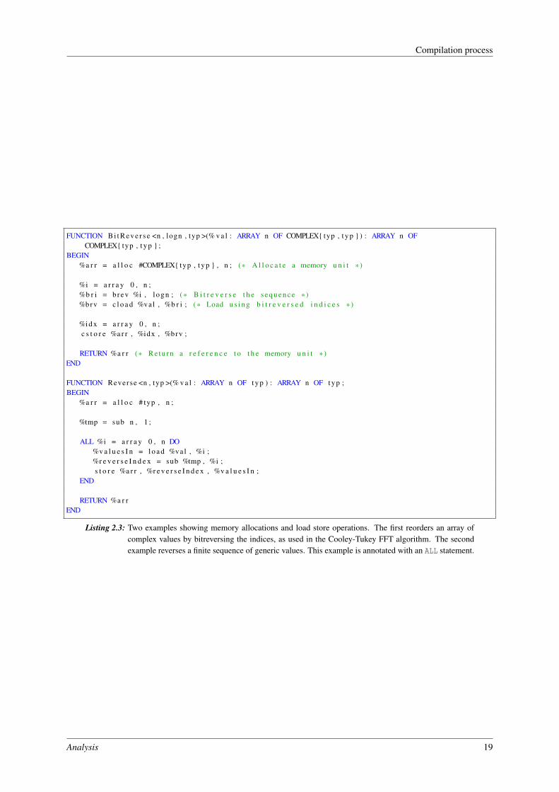
Two small examples showing memory allocation and memory load/store operations can be seen in Listing 2.3.

In the first case a memory unit containing a number of complex values is allocated. Operations pertaining to com-plex values are usually prefixed with a c. For example, cload loads a complex value from a memory unit, andcstore stores a complex number.

2.7 Compilation process

In figure 2.5 the workflow of the proposed methodology is shown. The user inputs a high-level description of analgorithm to a high-level compiler which turns the code into an Intermediate Representation (IR) language.

The compiler then starts by doing simple optimizations on this IR, such as constant folding, strength reduction,etc. The goal is to remove as many unnecessary operations as possible, transform expensive operations into lessexpensive operations, or turn unsupported operations, such as floating-point operations or operations on complexnumbers, into constants or integer math operations.

When the simple optimizations are done the tree should be reduced to a reasonably optimized form. At thispoint the compiler should try to calculate some simple statistics about general throughput, and amount of memoryaccesses inside any loop structure. The goal of this step is for the compiler to decide at what points doing control-flow altering optimizations, such as loop unrolling or loop splitting, can be beneficial. Those operations will beexplained in section 2.8.1.

After this step the loop structure information is no longer necessary, and the tree of operations is flattened into asingle graph. This consists of simply stripping all control flow information nodes out of the graph.

When the graph has been flattened a simple process turns the graph representation into a data-flow graph, whichcan then be processed in the last step. By traversing each node of this graph estimates of throughput and delay canbe gathered. This is used for the final step where the number of instantiated memory blocks, and sizes of inlinebuffer sizes is determined, and the final graph is outputted as HDL code which can be synthesized directly to aspecific FPGA.

High-levelcompiler

CodeSimple OptimizationsIR Loop transformations

Flattening HDLBuffer and RAMheuristics

Data-flowgeneration

Figure 2.5: A functional overview of the process from source text to final FPGA program. The processes in thestippled box indicate the scope of this project.

The scope of this project is only the low-level compiler which processes an IR source file, and outputs an HDL

18 Analysis

Compilation process

FUNCTION B i t R e v e r s e <n , logn , typ >(% v a l : ARRAY n OF COMPLEX{ typ , t y p } ) : ARRAY n OFCOMPLEX{ typ , t y p } ;

BEGIN%a r r = a l l o c #COMPLEX{ typ , t y p } , n ; (* A l l o c a t e a memory u n i t * )

%i = a r r a y 0 , n ;%b r i = b rev %i , l ogn ; (* B i t r e v e r s e t h e s e q u e n c e * )%brv = c l o a d %val , %b r i ; (* Load u s i n g b i t r e v e r s e d i n d i c e s * )

%i d x = a r r a y 0 , n ;c s t o r e %a r r , %idx , %brv ;

RETURN %a r r (* Re tu rn a r e f e r e n c e t o t h e memory u n i t * )END

FUNCTION Reverse <n , typ >(% v a l : ARRAY n OF t y p ) : ARRAY n OF t y p ;BEGIN

%a r r = a l l o c # typ , n ;

%tmp = sub n , 1 ;

ALL %i = a r r a y 0 , n DO%v a l u e s I n = l o a d %val , %i ;%r e v e r s e I n d e x = sub %tmp , %i ;s t o r e %a r r , %r e v e r s e I n d e x , %v a l u e s I n ;

END

RETURN %a r rEND

Listing 2.3: Two examples showing memory allocations and load store operations. The first reorders an array ofcomplex values by bitreversing the indices, as used in the Cooley-Tukey FFT algorithm. The secondexample reverses a finite sequence of generic values. This example is annotated with an ALL statement.

Analysis 19

Heuristics

source file. It should be fairly easy to imagine that creating a high-level compiler which can translate a high-levellanguage, such as a subset of C or Matlab code, into this IR code would be possible.

2.7.1 IR processing

The syntax of the IR used was explained in section 2.6, but to make it easier to process, the compiler will initiallyparse the IR code and turn it into a directed acyclic graph. Each node in this graph represents an operation, aconstant, an input, or an output, and edges connecting nodes represent value dependencies.

The graph illustrated in figure 2.6 shows two such graphs, although this example only shows the overall structureof the operations.

+

-

-

*

%a %b

%c

0

4

return

+

-

<<

%a %b

2

return

%c

Figure 2.6: Two simplified IR graphs showing the structure of the TestSpecialized function in Listing 2.1. Thegraph on the left is shown just as it is parsed, and the graph on the right shows the same function afterit has been optimized using simple optimizations. The specific order of arguments is not shown in thisfigure.

2.8 Heuristics

The proposed heuristics are supposed to automatically calculate when a loop transformation should be applied. Itcan do this by estimating how much FPGA hardware is required to implement a given loop body, and how high athroughput the given loop body has.

2.8.1 Loop body heuristics

If a loop body is a candidate for loop transformations, as explained in section 2.8.2, the compiler will try to calculatea number of measures about it. Those measures are based on estimates about the hardware cost(loop_body_weight),and the slowest block in the loop body(loop_body_throughput). These measures are combined to make a single

20 Analysis

Heuristics

cost estimate of how complex a loop body is. By comparing this to a set limit, which can be adjusted by theprogrammer, the compiler can decide to either unroll or split the loop.

Hardware cost

The method used to estimate hardware cost is the method proposed in [5]. The method relies on statistics gatheredfrom synthesizing a large number of integer operations with different bitwidth configurations, and noticing theresulting hardware costs. By graphing the resulting data points, some simple approximations of the hardware costsbased on some simple parameters could be found. The synthesis was performed for a specific Xilinx FPGA, fromthe Spartan 3 family. This project will use the same FPGA, but the report indicated that the method could work onother FPGA architectures that share the same basic structure.

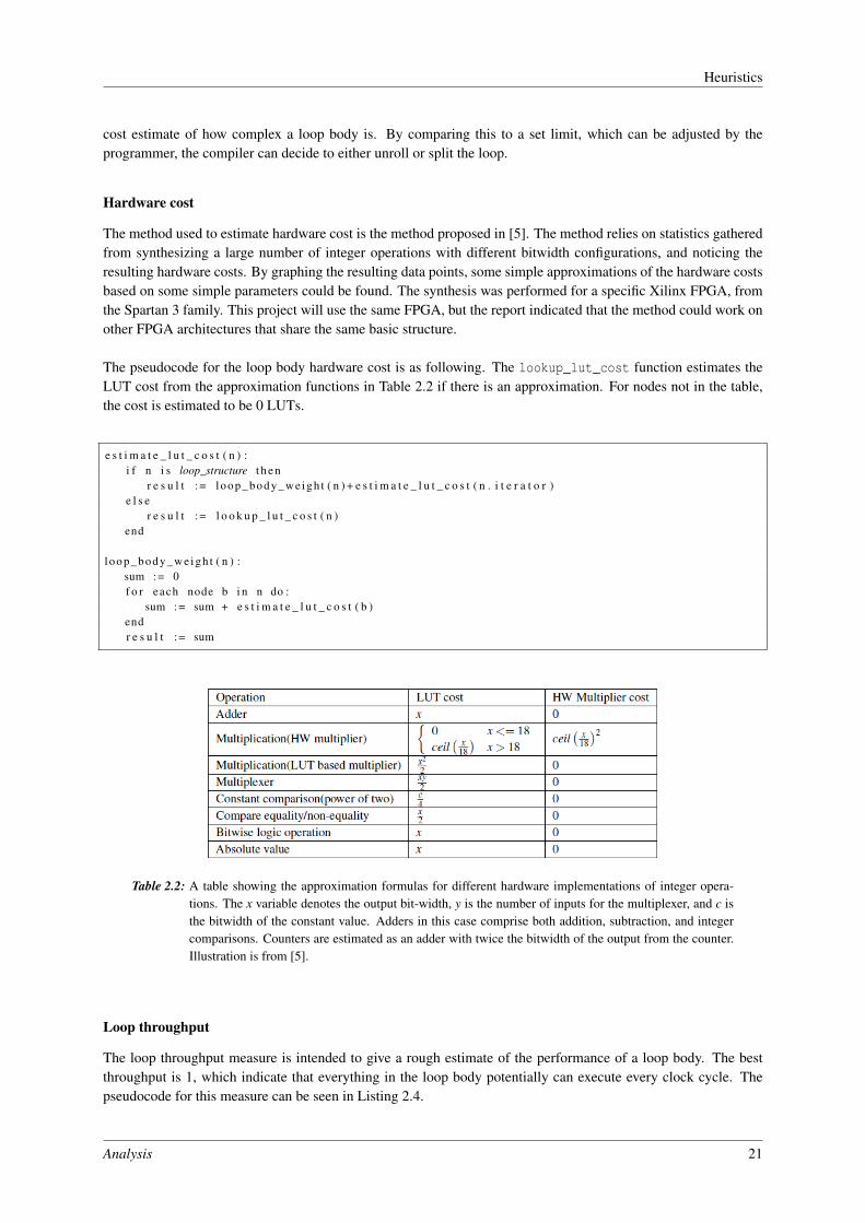
The pseudocode for the loop body hardware cost is as following. The lookup_lut_cost function estimates theLUT cost from the approximation functions in Table 2.2 if there is an approximation. For nodes not in the table,the cost is estimated to be 0 LUTs.

e s t i m a t e _ l u t _ c o s t ( n ) :i f n i s loop_structure t h e n

r e s u l t := loop_body_we igh t ( n ) + e s t i m a t e _ l u t _ c o s t ( n . i t e r a t o r )e l s e

r e s u l t := l o o k u p _ l u t _ c o s t ( n )end

loop_body_we igh t ( n ) :sum := 0f o r each node b i n n do :

sum := sum + e s t i m a t e _ l u t _ c o s t ( b )endr e s u l t := sum

Table 2.2: A table showing the approximation formulas for different hardware implementations of integer opera-tions. The x variable denotes the output bit-width, y is the number of inputs for the multiplexer, and c isthe bitwidth of the constant value. Adders in this case comprise both addition, subtraction, and integercomparisons. Counters are estimated as an adder with twice the bitwidth of the output from the counter.Illustration is from [5].

Loop throughput

The loop throughput measure is intended to give a rough estimate of the performance of a loop body. The bestthroughput is 1, which indicate that everything in the loop body potentially can execute every clock cycle. Thepseudocode for this measure can be seen in Listing 2.4.

Analysis 21

Heuristics

t h r o u g h p u t _ m i n ( n ) :i f ninputs = 0 t h e n

r e s u l t := 1e l s e

r e s u l t := minimum of t h r o u g h p u t ( b ) where b i s t h e node c o n n e c t e d t o n . inputi f o r a l l iend

t h r o u g h p u t ( n ) :i f ( n i s load_unit ) o r ( n i s store_unit ) t h e n

tmp := number o f l o a d and s t o r e p o r t s o f t h e memory u n i t w i th p r i o r i t y >n . l o a d p o r t . p r i o r i t y

i f tmp < 2 t h e nr e s u l t := 1

e l s er e s u l t := t h r o u g h p u t _ m i n ( n ) / ( tmp−1)

ende l s e i f n i s sum_unit t h e n

r e s u l t := t h r o u g h p u t _ m i n ( n ) *ninputs / c o u n te l s e

r e s u l t := t h r o u g h p u t _ m i n ( n )end

l o o p _ b o d y _ t h r o u g h p u t ( n ) :r e s u l t := minimum of t h r o u g h p u t ( b ) where b i s each node i n n

Listing 2.4: Pseudocode for the throughput measure functions.

Combined measure, and transform descision

The final measure is simply a product of loop_body_throughput(n) and loop_body_weight(n) where n isthe loop node. The goal is to optimize the nodetree without having this measure exceed a given maximum. Onestrategy could be to select the loop in the nodetree with the worst score, and optimize that first, and then move onto the next, and continue this until all loops have been visited.

When visiting a loop it is first investigated whether it satisfies the loop transform condition.If it does, the combined measure is calculated, and if it exceeds the given maximum the compiler must try to splitthe loop in a way that makes it not exceed the maximum.

2.8.2 Loop transformations

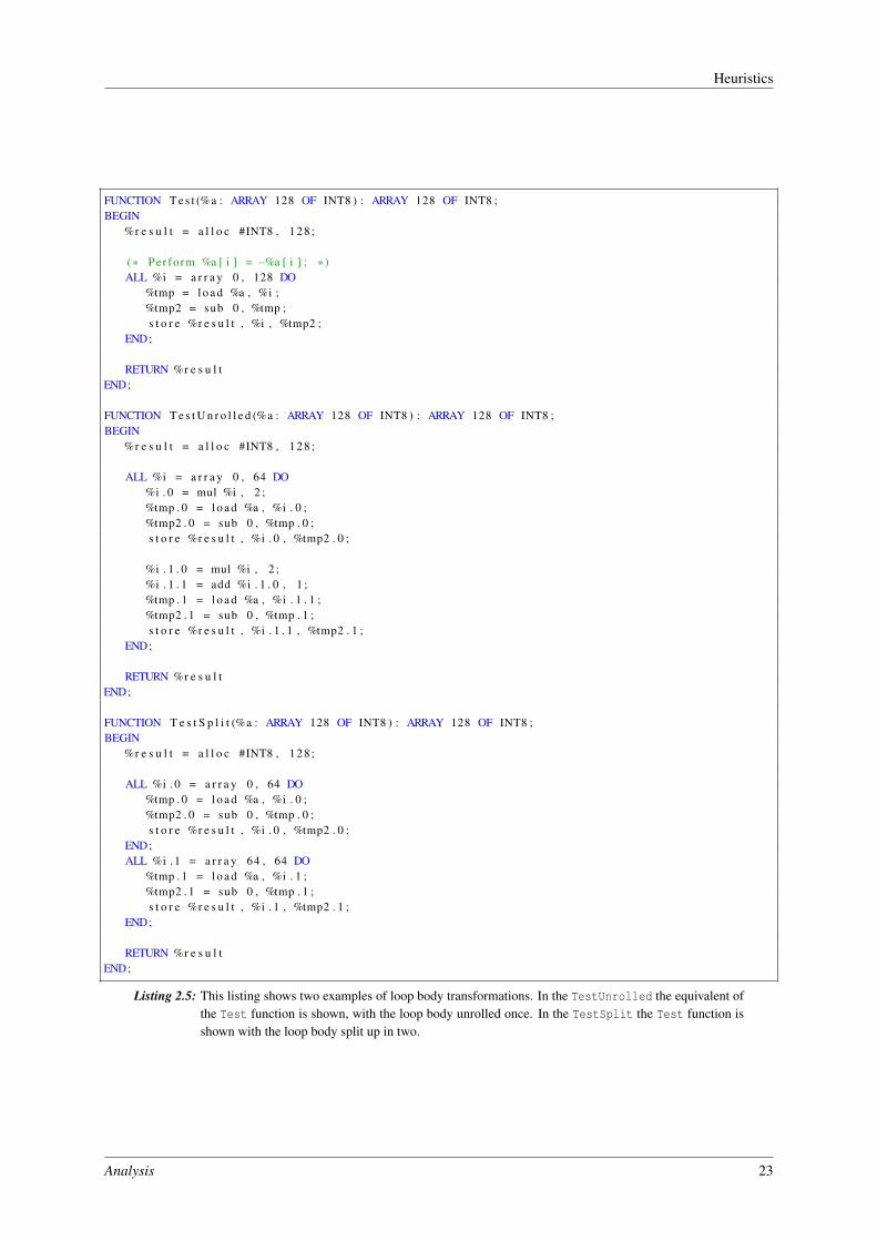
Loop unrolling means replicating the operations inside a loop a number of times, and adjusting the loop counterfor each replicated loop body. The number of times must be an integer factor of the total amount of loop iterationsin the original loop. E.g. if a loop body processes some data with an loop counter of i, then unrolling that loopby a factor of 4 would mean duplicating the loop body 4 times inside the loop, dividing the number of iterationsof the loop counter by 4, and replacing the loop counter reference in each duplicated loop body with respectivelyi∗4+0, i∗4+1, i∗4+2, and i∗4+3.Loop splitting is the process of creating two new loop structures as copies of an old loop structure where the newones only process half of the old loops range.Listing 2.5 shows examples of those two loop body transformations.

Loop unrolling

The reason loop unrolling can be a useful optimization in FPGA fabric is that it replicates operations that are"close" to each other. This can be good if the code generating values for the operations in a loop can maintain ahigh throughput.

22 Analysis

Heuristics

FUNCTION T e s t (%a : ARRAY 128 OF INT8 ) : ARRAY 128 OF INT8 ;BEGIN

%r e s u l t = a l l o c #INT8 , 128 ;

(* Per fo rm %a [ i ] = −%a [ i ] ; * )ALL %i = a r r a y 0 , 128 DO

%tmp = l o a d %a , %i ;%tmp2 = sub 0 , %tmp ;s t o r e %r e s u l t , %i , %tmp2 ;

END;

RETURN %r e s u l tEND;

FUNCTION T e s t U n r o l l e d (%a : ARRAY 128 OF INT8 ) : ARRAY 128 OF INT8 ;BEGIN

%r e s u l t = a l l o c #INT8 , 128 ;

ALL %i = a r r a y 0 , 64 DO%i . 0 = mul %i , 2 ;%tmp . 0 = l o a d %a , %i . 0 ;%tmp2 . 0 = sub 0 , %tmp . 0 ;s t o r e %r e s u l t , %i . 0 , %tmp2 . 0 ;

%i . 1 . 0 = mul %i , 2 ;%i . 1 . 1 = add %i . 1 . 0 , 1 ;%tmp . 1 = l o a d %a , %i . 1 . 1 ;%tmp2 . 1 = sub 0 , %tmp . 1 ;s t o r e %r e s u l t , %i . 1 . 1 , %tmp2 . 1 ;

END;


FUNCTION T e s t S p l i t (%a : ARRAY 128 OF INT8 ) : ARRAY 128 OF INT8 ;BEGIN

%r e s u l t = a l l o c #INT8 , 128 ;

ALL %i . 0 = a r r a y 0 , 64 DO%tmp . 0 = l o a d %a , %i . 0 ;%tmp2 . 0 = sub 0 , %tmp . 0 ;s t o r e %r e s u l t , %i . 0 , %tmp2 . 0 ;

END;ALL %i . 1 = a r r a y 64 , 64 DO

%tmp . 1 = l o a d %a , %i . 1 ;%tmp2 . 1 = sub 0 , %tmp . 1 ;s t o r e %r e s u l t , %i . 1 , %tmp2 . 1 ;

END;


Listing 2.5: This listing shows two examples of loop body transformations. In the TestUnrolled the equivalent ofthe Test function is shown, with the loop body unrolled once. In the TestSplit the Test function isshown with the loop body split up in two.

Analysis 23

Heuristics

There are many reasons why it might not be a good optimization though. If the code preceeding the loop body,which generates values that are used in the loop body cannot keep up, the effect of loop unrolling might be thecomplete opposite. Now the loop has to wait for each added iteration while the others might have nothing to do,which lowers the utilization and unnecessarily raises the complexity of the code.

Loop splitting

This loop body transformation is very interesting, since it does not change the body of the loop but only changesthe loop bounds. Another potential benefit of this optimization could be in cases where loops just iterate linearlyover a memory address range. By splitting the loop body strategically the iterations might be split up in a waywhere each loop body only has to reference a specific part of an array. If the array was constructed in a numberof consecutive block RAMs those could be split up and each side be reserved for each new loop body. This essen-tially doubles the number of reads or writes that could be performed at a time, theoretically scaling the memorythroughput by 2. Only ALL loops can be splitted.

In the TestSplit function in listing 2.5 the two new loops only access the lower and upper 64 elements of the%result array respectively. This means that if the array was allocated as two 64 element block RAMs, the twoloops could have exclusive access to one of those block RAMs.

Transformation conditions, and sum node duplication

To be a candidate for loop transformations the operations inside the loop may only read and write to memory units,and any value calculated inside whose result is used outside the loop body must be a sum operation. Memory unitallocations are the only operations where it is permitted for the result to be used outside the loop body where it hasbeen allocated.

Those conditions are necessary since simple operations cannot easily be split up into more loops, or be splicedtogether again.

When a sum operation is split up the compiler must insert a new sum operation right after the loop body, whichaccumulates the original sum result, and the newly added sum results. This new sum operation must have a countof the number of times the loop was split or unrolled.Likewise, each sum operation inside the loop body, which depends either directly or indirectly on the loop iteratorvariable must have its count divided by the number of times the loop was split or unrolled.

24 Analysis

3Specification

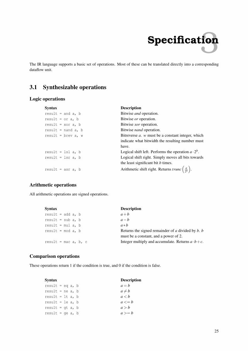
The IR language supports a basic set of operations. Most of these can be translated directly into a correspondingdataflow unit.

3.1 Synthesizable operations

Logic operations

Syntax Descriptionresult = and a, b Bitwise and operation.result = or a, b Bitwise or operation.result = xor a, b Bitwise xor operation.result = nand a, b Bitwise nand operation.result = brev a, w Bitreverse a. w must be a constant integer, which

indicate what bitwidth the resulting number musthave.

result = lsl a, b Logical shift left. Performs the operation a ·2b.result = lsr a, b Logical shift right. Simply moves all bits towards

the least significant bit b times.

result = asr a, b Arithmetic shift right. Returns trunc(

a2b

).

Arithmetic operations

All arithmetic operations are signed operations.

Syntax Descriptionresult = add a, b a+bresult = sub a, b a−bresult = mul a, b a∗bresult = mod a, b Returns the signed remainder of a divided by b. b

must be a constant, and a power of 2.result = mac a, b, c Integer multiply and accumulate. Returns a ·b+c.

Comparison operations

These operations return 1 if the condition is true, and 0 if the condition is false.

Syntax Descriptionresult = eq a, b a = bresult = ne a, b a 6= bresult = lt a, b a < bresult = le a, b a <= bresult = gt a, b a > bresult = ge a, b a >= b

25

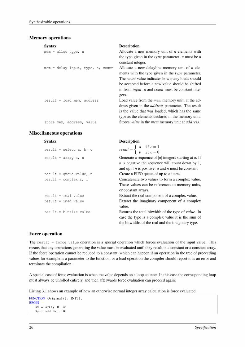
Synthesizable operations

Memory operationsSyntax Descriptionmem = alloc type, n Allocate a new memory unit of n elements with

the type given in the type parameter. n must be aconstant integer.

mem = delay input, type, n, count Allocate a new delayline memory unit of n ele-ments with the type given in the type parameter.The count value indicates how many loads shouldbe accepted before a new value should be shiftedin from input. n and count must be constant inte-gers.

result = load mem, address Load value from the mem memory unit, at the ad-dress given in the address parameter. The resultis the value that was loaded, which has the sametype as the elements declared in the memory unit.

store mem, address, value Stores value in the mem memory unit at address.

Miscellaneous operationsSyntax Description

result = select a, b, c result ={

a if c = 1b if c = 0

result = array a, n Generate a sequence of |n| integers starting at a. Ifn is negative the sequence will count down by 1,and up if n is positive. a and n must be constant.

result = queue value, n Create a FIFO queue of up to n items.result = complex r, i Concatenate two values to form a complex value.

These values can be references to memory units,or constant arrays.

result = real value Extract the real component of a complex value.result = imag value Extract the imaginary component of a complex

value.result = bitsize value Returns the total bitwidth of the type of value. In

case the type is a complex value it is the sum ofthe bitwidths of the real and the imaginary type.

Force operation

The result = force value operation is a special operation which forces evaluation of the input value. Thismeans that any operations generating the value must be evaluated until they result in a constant or a constant array.If the force operation cannot be reduced to a constant, which can happen if an operation in the tree of preceedingvalues for example is a parameter to the function, or a load operation the compiler should report it as an error andterminate the compilation.

A special case of force evaluation is when the value depends on a loop counter. In this case the corresponding loopmust always be unrolled entirely, and then afterwards force evaluation can proceed again.

Listing 3.1 shows an example of how an otherwise normal integer array calculation is force evaluated.

FUNCTION O r i g i n a l ( ) : INT32 ;BEGIN

%x = a r r a y 0 , 4 ;%y = add %x , 1 0 ;

26 Specification

Helper operations

%z = f o r c e %y ;%w = sum %z , 4 ;RETURN %w

END

FUNCTION Fixed ( ) : INT32 ;BEGIN

%x = <INT3 : 0 , 1 , 2 , 3 >; (* Array i s f o r c e d i n t o a c o n s t a n t a r r a y * )%y = <INT5 : 10 , 11 , 12 , 13 >;%z = <INT5 : 10 , 11 , 12 , 13 >;%w = 4 6 ; (* The sum of a c o n s t a n t a r r a y i s c o n s t a n t * )RETURN %w

END

Listing 3.1: Evaluation of a force operation. The Original shows a function before force evaluation, and Fixed

shows the same function after evaluation.

3.2 Helper operations

Helper operations are operations that are not real operations, but rather a series of more primitive often used oper-ations. The common case is that of complex operations, which can be decomposed into basic operations, and thenassembled into complex again.

Syntax Equivalent operationresult = cload mem, address

%tmp . 0 = r e a l mem;%tmp . 1 = imag mem;%tmp . r = l o a d %tmp . 0 , a d d r e s s ;%tmp . i = l o a d %tmp . 1 , a d d r e s s ;%tmp . 2 = complex %tmp . r , %tmp . i ;r e s u l t = %tmp . 2 ;

cstore mem, address, value

%tmp . 0 = r e a l mem;%tmp . 1 = imag mem;%tmp . 2 = r e a l v a l u e ;%tmp . 3 = imag v a l u e ;s t o r e %tmp . 0 , a d d r e s s , %tmp . 2 ;s t o r e %tmp . 1 , a d d r e s s , %tmp . 3 ;

result = cadd a, b

%tmp . 0 = r e a l a ;%tmp . 1 = imag a ;%tmp . 2 = r e a l b ;%tmp . 3 = imag b ;%tmp . 4 = add %tmp . 0 , %tmp . 2 ;%tmp . 5 = add %tmp . 1 , %tmp . 3 ;%tmp . 6 = complex %tmp . 4 , %tmp . 5 ;r e s u l t = %tmp . 6 ;

Specification 27

Floating point operations

result = csub a, b

%tmp . 0 = r e a l a ;%tmp . 1 = imag a ;%tmp . 2 = r e a l b ;%tmp . 3 = imag b ;%tmp . 4 = sub %tmp . 0 , %tmp . 2 ;%tmp . 5 = sub %tmp . 1 , %tmp . 3 ;%tmp . 6 = complex %tmp . 4 , %tmp . 5 ;r e s u l t = %tmp . 6 ;

result = cmul a, b

%tmp . 0 = r e a l a ;%tmp . 1 = imag a ;%tmp . 2 = r e a l b ;%tmp . 3 = imag b ;%tmp . 4 = mul %tmp . 0 , %tmp . 2 ;%tmp . 5 = mul %tmp . 1 , %tmp . 3 ;%tmp . 6 = sub %tmp . 4 , %tmp . 5 ;%tmp . 7 = mul %tmp . 0 , %tmp . 3 ;%tmp . 8 = mul %tmp . 1 , %tmp . 2 ;%tmp . 9 = add %tmp . 7 , %tmp . 8 ;%tmp . 1 0 = complex %tmp . 6 , %tmp . 9 ;r e s u l t = %tmp . 1 0 ;

result = casr a, n

%tmp . 0 = r e a l a ;%tmp . 1 = imag a ;%tmp . 2 = a s r %tmp . 0 , n ;%tmp . 3 = a s r %tmp . 1 , n ;%tmp . 4 = complex %tmp . 2 , %tmp . 3 ;r e s u l t = %tmp . 4 ;

result = cmod a, n

%tmp . 0 = r e a l a ;%tmp . 1 = imag a ;%tmp . 2 = mod %tmp . 0 , n ;%tmp . 3 = mod %tmp . 1 , n ;%tmp . 4 = complex %tmp . 2 , %tmp . 3 ;r e s u l t = %tmp . 4 ;

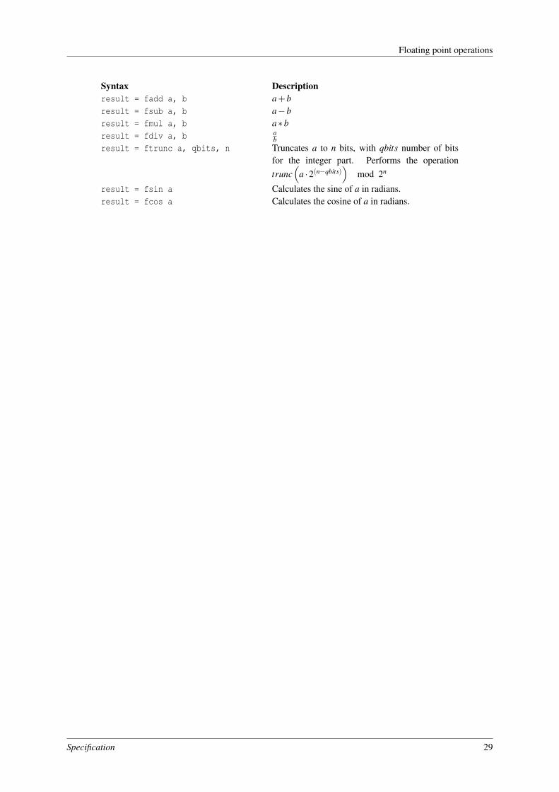
3.3 Floating point operations

Floating point operations cannot be synthesized and will always be force evaluated. The precision of the floatingpoint value is implementation dependant.

28 Specification


Syntax Descriptionresult = fadd a, b a+bresult = fsub a, b a−bresult = fmul a, b a∗bresult = fdiv a, b a

bresult = ftrunc a, qbits, n Truncates a to n bits, with qbits number of bits

for the integer part. Performs the operationtrunc

(a ·2(n−qbits)

)mod 2n

result = fsin a Calculates the sine of a in radians.result = fcos a Calculates the cosine of a in radians.

Specification 29


30 Specification

4Implementation

4.1 Compiler

4.1.1 Structure

Figure 4.1 shows the structure of the compiler implementation in this project.

The input to the compiler is a set of files with IR code. This code is first processed by the scanner and the parser,which generate a nodetree. The nodetree is essentially just a hierachical list of the instructions in the IR code,stored in a way which makes it easy to modify the order, operations, and values of each operation.

Since the IR is centric about functions, the operations are only processed per static function in the source file;however, one of the first tasks of the compiler after creating the nodetree is to inline all function-calls. This meansthat the content of the called function is directly copied into the place where it was called. The function-call argu-ments and parameters are directly replaced, and the function call result is assigned to the return statement of thefunction called. This means that after all function-calls have been inlined the processed function will be a largeself-contained function.

The function-inlining step is just one of many in the optimization process. These optimization processes will berepeated for the function node-tree until nothing is changed in the tree. At that point the optimization is done.

At this point bit-width estimation is performed for each node. This step estimates how many bits should be usedin the output of an operation node to safely store the result of the operation. Since this is only an estimation theresult will not be very precise, but the estimate will provide the baseline for the resource estimates in the looptransform step. The loop transform step will try to split or unroll loops that are estimated to improve performancein the graph. If the step succeeds in transforming one or more loops the optimization process starts over with thenew nodetree. If the loop transform step does not modify anything in the tree the entire optimization is complete,and the tree is flattened, which means all control flow information is stripped from the tree, and the hierarchicalnode-tree is turned into a simple list of nodes.

The last step, before generating the synthesizable Verilog code, is to generate a final DFG which involves replacingall high-level operations in the nodetree with low-level functional units. With the selected set of operations, thiscurrently only involves replacing loop counters with simple cascaded counters.

Finally the Verilog code is emitted, which can be compiled synthesized directly. After synthesis of the generatedHDL code, most modern synthesis tools are very good at optimizing away superfluous bits in calculations.

4.1.2 Scanner and parser

Scanner

The scanners job is to convert a stream of characters into a stream of tokens. A token is a pair of a symbol identifier,and the string which comprised the token. A symbol identifier could for example be a number, a semicolon, anidentifier, or a left parentheses. The design of the scanner is based on the method described in [11].

The distinction between a scanner and the parser is that the scanner provides very basic parsing of input characters,and groups them together to form either symbols, identifiers, keywords, or numbers. An identifier is a sequenceof letters and digits, which has to start with a letter. This way it can easily be distinguished from numbers and

31

Compiler

symbols. Keywords are certain identifiers which has a specific meaning for the language, and thus cannot be usedas names.

For example, the following arbitrary text "FUNCTION 2+2.3E-5; (2+1)" will be turned into the following tokenstream tkFunction, tkInteger(2), tkPlus, tkReal(2.3E-5), tkSemicolon, tkLParen, tkInteger(2), tkPlus, tkIn-teger(1), tkRParen. The symbol identifiers are prefixed with tk, and the string generating the token is enclosed inthe following parentheses if the token is an integer, real, or an identifier.

Parser

The parser receives the tokens from the scanner, and by interpreting them based on a set of hierarchical rules canconstruct a tree which describes the original character data. The rules can be seen in Appendix A.1, where it isdenoted in EBNF (Extended Bachus-Naur Form) [11]. The parser is implemented as a recursive-descent parser,since the syntax is fairly simple.

The parser starts parsing at the beginning of a file, by applying the module rule. If at some point in the tokenstream, an unexpected token is received the compiler should give up further parsing and report a syntax error.

For example, if the parser was applying the Statement rule to the text "ALL %x = 5 DO END", the parser wouldapply the following rules: Statement, AllStatement, Variable, Ident, "=". After this it would give up since it wasexpecting a command to follow the equal sign. The Command expected an Ident, but got an Integer.

4.1.3 Constant propagation

The concept behind constant propagation is to forward known constants into all following operations. This allowsthe compiler to potentially collapse operations into constants which again can facilitate further constant propa-gation. This optimization step is rather important since it removes many potentially wasteful operations in thenodetree, which might not give a clear picture of how the synthesized FPGA firmware will behave. FPGA syn-thesis tools are good at automatically removing and propagating constants in RTL descriptions. Having a nodetreethat maps closely to an actual FPGA firmware makes it possible to run heuristics on it that actually may reflect theactual outcome of any nodetree transformations.

4.1.4 Operation simplification

This step, also known as strength reduction, collapses operations into constants, or replaces complex operationswith simpler operations. For example, listing 4.1 shows two functions. In func2, func1 has been simplified andconstants have been propagated.

4.1.5 Unused code removal

This step is very simple, in that it simply iterates over all operations in a function and marks variables that areread somewhere. After this, the compiler iterates over all known variables that are assigned in the program, andremoves any operation that are not marked as used, unless the operation has visible sideeffects for the rest of theprogram.

This could be the case of load units, which mark certain positions in a memory block as read. Removing this blockwould mean that any store unit which tries to write more times to that block would fail, and the program would bebroken.

32 Implementation

Compiler

FUNCTION func1 (%x : INT32 ) : INT32 ;BEGIN

%0 = add %x , 0 ;%1 = mul 10 , −2;%2 = sub %0, %x ;%3 = sub %2, %1;RETURN %3

END


%0 = %x :%1 = −20;%2 = 0 ;%3 = 2 0 ;RETURN 20

END


RETURN 20END

Listing 4.1: Example of a function after repeated simplification, constant propagation, and unused code removal.func1 shows the original, func2 shows the function after 4 steps of simplificiation and constantpropagation, and func3 shows func2 after all unused code has been removed.

4.1.6 Loop counter insertion

Loop counters are a special value type which is useful for propagating certain iterator indices inside loop bodies.Inside loops any reference to the loop iterators will be replaced by a loop counter value.

Loop counters are denoted as { wn−1, ..., w0 | offset }, where wx indicate the weight of the x’th level ofthe loop iterator variable, where 1 corresponds to the innermost loop. The final value of the loop counter value isgiven as ∑

ni=0 wiCi +o f f set, where Ci is the value of the i’th iterator variable.

Loop counters can be propagated as constants, to some degree, since they correspond to a linear function of allloop iterators in the context. For example, adding 2 to a loop counter will simply add 2 to w0. Multiplying by aconstant integer will scale all wi by that factor.

When generating the final DFG these loop counters can be replaced by n cascaded counter units, properly config-ured with scaled steps according to the new weight. On one hand this create more duplicated functionality, butit was found in experiments that this was almost always beneficial for generating better overall execution speedperformance.

Listing 4.2 shows an example of a function which uses two levels of ALL loops. In func1 the original function isshown, while in func2 references to the loop counter have been replaced. In func3 the loop counters are simplified,and propagated into the following operations by the simplification and constant propagation process. Finally, afterflattening and unused code removal, as shown in func4, all loop counters and the values %0 and %1 have beenremoved since they were no longer referenced. The loop counters have been replaced by counters, which matchthe original loop iterator value in length and start value, but with steps that match the weights of the loop counters.

Implementation 33

Compiler

FUNCTION func1 ( ) : INT32 ;BEGIN

ALL %x = a r r a y 0 , 4 DOALL %y = a r r a y 0 , 4 DO

%0 = mul %y , 4 ;%1 = add %0, %x ;%2 = sum %1, 4 ;

END%3 = add %x , %2;

END

RETURN %3END



%0 = mul { 0 , 1 | 0 } , 4 ;%1 = add %0, { 1 , 0 | 0 } ;%2 = sum %1, 4 ;

END%3 = add { 1 | 0 } , %2;

END

RETURN %3END



%0 = { 0 , 4 | 0 } ;%1 = { 1 , 4 | 0 } ;%2 = sum { 1 , 4 | 0 } , 4 ;

END%3 = add { 1 | 0 } , %2;

END

RETURN %3END


%2. tmp . 1 = i n n e r c o u n t 0 , 4 , 4 ;%2. tmp . 2 = o u t e r c o u n t 0 , 1 , 4 , %2. tmp . 1 ;%2 = sum %2. tmp . 2 , 4 ;

%3. tmp . 1 = i n n e r c o u n t 0 , 1 , 4 ;%3 = add %3. tmp . 1 , %2;

RETURN %3END

Listing 4.2: An example of loop counter insertion, and the following simplification, constant propagation, unusedcode removal, and flattening. The innercount and outercount operations are simply a textualrepresentation of the nodes created.

34 Implementation

Compiler

4.1.7 Bit-width analysis

The task of determining bitwidths is performed using a combination of Affine Arithmetic (AA) and Interval Arith-metic (IA) [10]. In FPGA-Oberon this task was done with a simple method which has many similarities withInterval Arithmetic, which performed well enough for very simple programs, but in many cases would yield bit-widths that were very pessimistic. AA tries to give a more informative picture of the ranges required by a networkof math operations by expressing intermediate results as a weighted sum of uniformly distributed stochastic vari-ables, which are correlated with inputs and factors in the calculation.

What the end product of this step is, is that each operations outputs in a nodetree has an associated range of possibleinteger values it can conceivably have. The output of an addition node would have a range that was a function ofthe two inputs. A range is denoted with the syntax [a__b] where a, and b are the lowest and highest integer valuethe number can have respectively. These calculations are done on real numbers, so before the final ranges are usedthey are rounded down and up to contain all the integers in the indicated range.

The method used in this implementation uses a combination of AA and IA. Both algorithms are applied to theentire design, and then afterwards the compiler iterates over all nodes and selects the most optimistic estimate.

For simplicity’s sake the following description will not take floating point rounding into account when explainingconcepts, but the actual implementation correctly takes those effects into account as proposed in [10].In IA it is simple to figure out the ranges of linear operations. For example, given two ranges [a__b] and [c__d],their sum would yield a range of [a+ c__b+ d]. In AA a range is defined as ∑

ni=1 wiεi +w0, where wi is a real

number, and εi is a uniformly distributed number with a range of [−1__1]. The important thing is that the stochasticvariables are global to all nodes, and that they are propagated through the system. Finding the IA range of an AArange, can be done as this:

radius =n

∑i=1|wi|

range = [(w0− radius)__(w0 + radius)]

For example, given two ranges in AA form: 1.3ε1 + 0.5 and 2.5ε1− 50.0ε2 + 2.0 the resulting sum would be(1.3+2.5)ε1−50.0ε2 +2.5, and the range of that would be [−51.3__56.3].

The example in listing 4.3 shows two functions that calculate (x+5)(5−x) where x is a 3-bit signed integer givingit a range of [−4__3]. Using IA, the resulting range estimate is [2__72], and for AA the result is [9__40.5]. Bydoing the calculation by hand it is found that the actual range is [9__25]. In this example AA finds the lowestbound correctly, and is almost 2 times better than IA in finding the upper bound.

After finding the ranges, the bits required to represent a range [a__b] can be calculated as:

vmax = max(a,b)

bits =

dlog2(vmax)e+1 vmax > 0dlog2 (−vmax)e+1 vmax < 00 vmax = 0

4.1.8 Verilog code generation

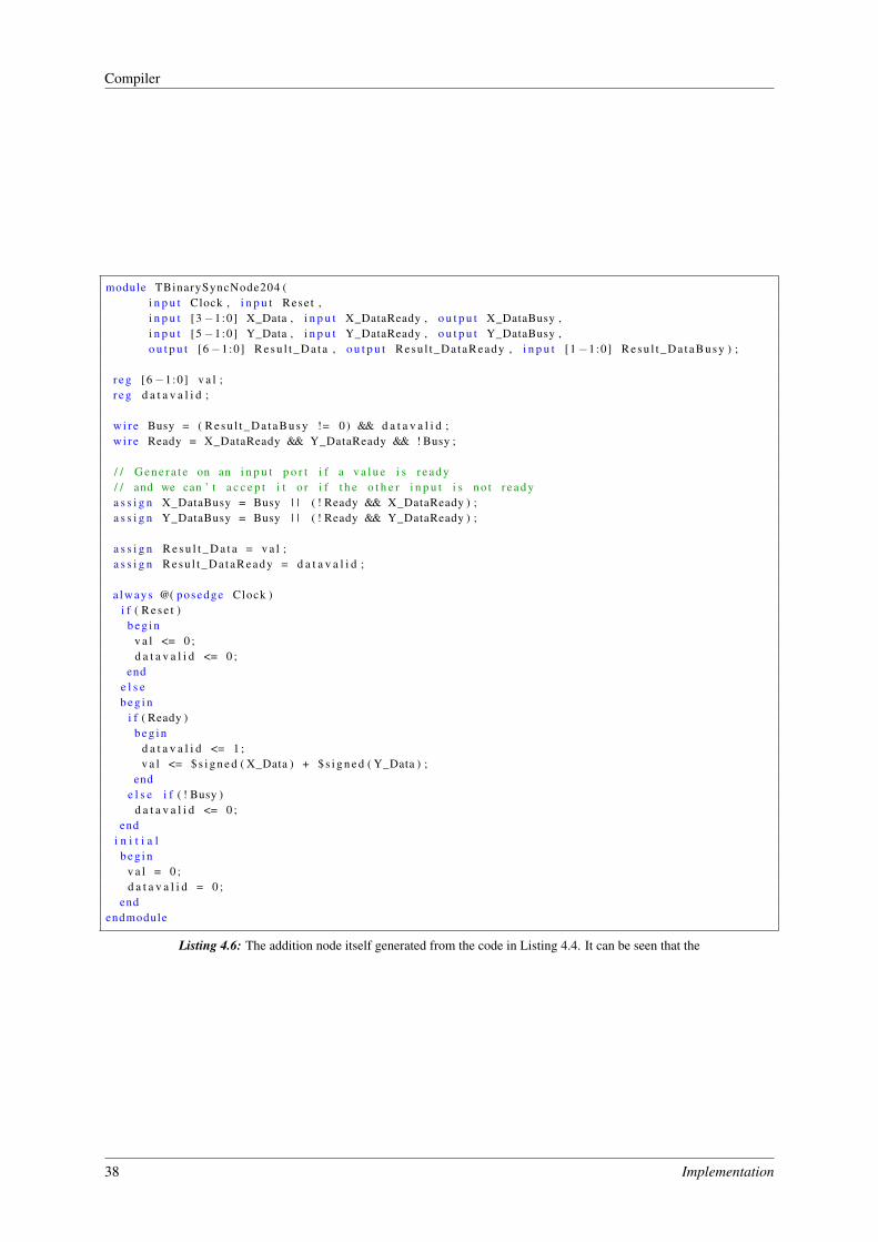
Since all code is limited to a small set of operations, the code to generate the Verilog code is simply hardcodedinto the compiler. Due to lack of time the compiler will generate a specialized module for each functional unit,and dump all specialized modules into a single file. Finally it will generate a main module, which contains all thewires to tie inputs to outputs in instances of the specialized modules. This is quite inefficient, and generate very

Implementation 35

Compiler

FUNCTION IA(%x : INT3 ) : INT32 ;BEGIN

(* %x = [−4__3 ] * )%0 = add %x , 5 ; (* %0 = [1 __8 ] * )%1 = sub 10 , %0; (* %1 = [2 __9 ] * )%2 = mul %0, %1; (* %2 = [2 __72 ] * )RETURN %2

END

FUNCTION AA(%x : INT3 ) : INT32 ;BEGIN

(* %x = −0.5+3.5ε0 *)%0 = add %x , 5 ; (* %0 = 4 . 5 + 3 . 5 ε0 *)%1 = sub 10 , %0; (* %1 = 5.5−3.5ε0 *)%2 = mul %0, %1; (* %2 = 2 4 . 7 5 + 3 . 5 ε0 +12.25ε1 = [9 __40 . 5 ] * )RETURN %2

END

Listing 4.3: Two identical functions with comments added which contains the estimated intervals of the operationusing IA and AA.

large source files, and could easily have been designed to be more flexible given more time.

In listing 4.4 a simple function is shown. Given its simplicity the optimization can do nothing to reduce it.

FUNCTION T e s t (%x : INT3 ; %y : INT5 ) : INT6 ;BEGIN

%tmp = add %x,%y ;RETURN %tmp

END

Listing 4.4: Simple function consisting of an adder.

36 Implementation

Compiler

module TInputSyncNode202 (i n p u t Clock , i n p u t Rese t ,i n p u t [3−1:0] x_Data , i n p u t x_DataReady , o u t p u t x_DataBusy ,o u t p u t [3−1:0] R e s u l t _ D a t a , o u t p u t Resu l t_DataReady , i n p u t [1−1:0] Resu l t _Da taBusy ) ;

a s s i g n R e s u l t _ D a t a = x_Data ;a s s i g n Resu l t_Da taReady = x_DataReady ;a s s i g n x_DataBusy = ( Resu l t _Da taBusy != 0) ;

endmodule

module TInputSyncNode203 (i n p u t Clock , i n p u t Rese t ,i n p u t [5−1:0] y_Data , i n p u t y_DataReady , o u t p u t y_DataBusy ,o u t p u t [5−1:0] R e s u l t _ D a t a , o u t p u t Resu l t_DataReady , i n p u t [1−1:0] Resu l t _Da taBusy ) ;

a s s i g n R e s u l t _ D a t a = y_Data ;a s s i g n Resu l t_Da taReady = y_DataReady ;a s s i g n y_DataBusy = ( Resu l t _Da taBusy != 0) ;

endmodule

module TOutputSyncNode205 (i n p u t Clock , i n p u t Rese t ,i n p u t [6−1:0] r e t u r n v a l u e s _ D a t a , i n p u t r e t u r n v a l u e s _ D a t a R e a d y , o u t p u t

r e t u r n v a l u e s _ D a t a B u s y ,o u t p u t [6−1:0] R e s u l t _ D a t a , o u t p u t Resu l t_DataReady , i n p u t [1−1:0] Resu l t _Da taBusy ) ;

a s s i g n R e s u l t _ D a t a = r e t u r n v a l u e s _ D a t a ;a s s i g n Resu l t_Da taReady = r e t u r n v a l u e s _ D a t a R e a d y ;a s s i g n r e t u r n v a l u e s _ D a t a B u s y = ( Resu l t _Da taBusy != 0) ;

endmodule

Listing 4.5: Verilog code of the input and output nodes of the function in Listing 4.4. These objects only route wiresdirectly through, and are only there to simplify the Verilog code generation.

Implementation 37

Compiler

module TBinarySyncNode204 (i n p u t Clock , i n p u t Rese t ,i n p u t [3−1:0] X_Data , i n p u t X_DataReady , o u t p u t X_DataBusy ,i n p u t [5−1:0] Y_Data , i n p u t Y_DataReady , o u t p u t Y_DataBusy ,o u t p u t [6−1:0] R e s u l t _ D a t a , o u t p u t Resu l t_DataReady , i n p u t [1−1:0] Resu l t _Da taBusy ) ;

r e g [6−1:0] v a l ;r e g d a t a v a l i d ;

w i r e Busy = ( Resu l t _Da taBusy != 0) && d a t a v a l i d ;w i r e Ready = X_DataReady && Y_DataReady && ! Busy ;

/ / G e n e r a t e on an i n p u t p o r t i f a v a l u e i s r e a d y/ / and we can ’ t a c c e p t i t o r i f t h e o t h e r i n p u t i s n o t r e a d ya s s i g n X_DataBusy = Busy | | ( ! Ready && X_DataReady ) ;a s s i g n Y_DataBusy = Busy | | ( ! Ready && Y_DataReady ) ;

a s s i g n R e s u l t _ D a t a = v a l ;a s s i g n Resu l t_Da taReady = d a t a v a l i d ;

a lways @( posedge Clock )i f ( R e s e t )

b e g i nv a l <= 0 ;d a t a v a l i d <= 0 ;

ende l s eb e g i n

i f ( Ready )b e g i n

d a t a v a l i d <= 1 ;v a l <= $ s i g n e d ( X_Data ) + $ s i g n e d ( Y_Data ) ;

ende l s e i f ( ! Busy )

d a t a v a l i d <= 0 ;end

i n i t i a lb e g i n

v a l = 0 ;d a t a v a l i d = 0 ;

endendmodule

Listing 4.6: The addition node itself generated from the code in Listing 4.4. It can be seen that the

38 Implementation

Compiler

module Main (i n p u t Clock , i n p u t Rese t ,i n p u t [ 2 : 0 ] x_Data , i n p u t x_DataReady , o u t p u t x_DataBusy ,i n p u t [ 4 : 0 ] y_Data , i n p u t y_DataReady , o u t p u t y_DataBusy ,o u t p u t [ 5 : 0 ] R e s u l t _ D a t a , o u t p u t Resu l t_DataReady , i n p u t [ 0 : 0 ] Resu l t _Da taBusy ) ;

w i r e [ 2 : 0 ] TInpu tSyncNode202_Resu l tDa ta ;w i r e TInputSyncNode202_Resu l tDa taReady ;

w i r e [ 4 : 0 ] TInpu tSyncNode203_Resu l tDa ta ;w i r e TInputSyncNode203_Resu l tDa taReady ;

w i r e TBinarySyncNode204_XDataBusy ;w i r e TBinarySyncNode204_YDataBusy ;w i r e [ 5 : 0 ] TBinarySyncNode204_Resu l tDa ta ;w i r e TBinarySyncNode204_Resul tDataReady ;

w i r e TOutpu tSyncNode205_re tu rnva luesDa taBusy ;w i r e [ 5 : 0 ] TOutputSyncNode205_Resul tData ;w i r e TOutputSyncNode205_Resul tDataReady ;w i r e TOutputSyncNode205_Resul tDataBusy ;

a s s i g n R e s u l t _ D a t a = TOutpu tSyncNode205_Resul tData ;a s s i g n Resu l t_Da taReady = TOutputSyncNode205_Resul tDataReady ;a s s i g n TOutputSyncNode205_Resul tDataBusy = Resu l t _Da taBusy ;

TInputSyncNode202 TInputSyncNode202 ( . Clock ( Clock ) , . R e s e t ( R e s e t ) , . x_Data ( x_Data ) ,. x_DataReady ( x_DataReady ) , . x_DataBusy ( x_DataBusy ) ,. R e s u l t _ D a t a ( TInpu tSyncNode202_Resu l tDa ta ) ,. Resu l t_Da taReady ( TInputSyncNode202_Resu l tDa taReady ) ,. Resu l t _Da taBusy ( { TBinarySyncNode204_XDataBusy } ) ) ;

TInputSyncNode203 TInputSyncNode203 ( . Clock ( Clock ) , . R e s e t ( R e s e t ) , . y_Data ( y_Data ) ,. y_DataReady ( y_DataReady ) , . y_DataBusy ( y_DataBusy ) ,. R e s u l t _ D a t a ( TInpu tSyncNode203_Resu l tDa ta ) ,. Resu l t_Da taReady ( TInputSyncNode203_Resu l tDa taReady ) ,. Resu l t _Da taBusy ( { TBinarySyncNode204_YDataBusy } ) ) ;

TBinarySyncNode204 TBinarySyncNode204 ( . Clock ( Clock ) , . R e s e t ( R e s e t ) ,. X_Data ( TInpu tSyncNode202_Resu l tDa ta ) , . X_DataReady ( TInputSyncNode202_Resu l tDa taReady ) ,. X_DataBusy ( TBinarySyncNode204_XDataBusy ) , . Y_Data ( TInpu tSyncNode203_Resu l tDa ta ) ,. Y_DataReady ( TInputSyncNode203_Resu l tDa taReady ) ,. Y_DataBusy ( TBinarySyncNode204_YDataBusy ) , . R e s u l t _ D a t a ( TBinarySyncNode204_Resu l tDa ta ) ,. Resu l t_Da taReady ( TBinarySyncNode204_Resul tDataReady ) ,. Resu l t _Da taBusy ( { TOutpu tSyncNode205_re tu rnva luesDa taBusy } ) ) ;

TOutputSyncNode205 TOutputSyncNode205 ( . Clock ( Clock ) , . R e s e t ( R e s e t ) ,. r e t u r n v a l u e s _ D a t a ( TBinarySyncNode204_Resu l tDa ta ) ,. r e t u r n v a l u e s _ D a t a R e a d y ( TBinarySyncNode204_Resul tDataReady ) ,. r e t u r n v a l u e s _ D a t a B u s y ( TOutpu tSyncNode205_re tu rnva luesDa taBusy ) ,. R e s u l t _ D a t a ( TOutpu tSyncNode205_Resul tData ) ,. Resu l t_Da taReady ( TOutputSyncNode205_Resul tDataReady ) ,. Resu l t _Da taBusy ( { TOutputSyncNode205_Resul tDataBusy } ) ) ;

endmodule

Listing 4.7: The main module of the generated Verilog code. This module contains all instantiations andinput/output from the nodes in the nodetree of the code in Listing 4.4.

Implementation 39

Compiler

Figure 4.1: A block diagram showing all the processes run during compilation of an IR source file.

40 Implementation

5Test

5.1 FIR filter

To test the implementation a simple FIR filter is implemented and compared to the results gathered in [5]. There a16 tap FIR filter is compared to two version created with Xilinx inbuilt core generator.

At the time of testing, the compiler implementation did not support loop transformations, so those are performedby hand to show that the IR supports that.

The code for the FIR filter is:

FUNCTION FIR<n , typ >(% sample : t y p ; %c o e f : ARRAY n OF t y p ) : t y p ;BEGIN

%a = d e l a y %sample , n , n ;

ALL %3 = a r r a y 0 , n DO%4 = l o a d %a , %3;%5 = l o a d %coef , %3;%6 = mul %4, %5;%7 = sum %6, n ;

END

RETURN %7END

FUNCTION F i r I m p l (%x : INT16 ) : INT36 ;BEGIN

%y = FIR <16 ,# INT16>(%x , <INT8 : 6 ,0 ,−4 ,−3 ,5 ,6 ,−6 ,−13 ,7 ,44 ,64 ,44 ,7 ,−13 ,−6 ,6 >) ;RETURN %y

END

When unrolling the code fully, a nodetree resembling the following code is generated. This code has been writtenby hand since the compiler does not support automatic unrolling or splitting of loops.

FUNCTION F i r I m p l (%x : INT16 ) : INT36 ;BEGIN

%a = d e l a y %x , 16 , 1 6 ;

%c o e f = <INT8 : 6 ,0 ,−4 ,−3 ,5 ,6 ,−6 ,−13 ,7 ,44 ,64 ,44 ,7 ,−13 ,−6 ,6 >;

%a0 = l o a d %a , 0 ;%a1 = l o a d %a , 1 ;%a2 = l o a d %a , 2 ;%a3 = l o a d %a , 3 ;%a4 = l o a d %a , 4 ;%a5 = l o a d %a , 5 ;%a6 = l o a d %a , 6 ;%a7 = l o a d %a , 7 ;%a8 = l o a d %a , 8 ;%a9 = l o a d %a , 9 ;%a10 = l o a d %a , 1 0 ;%a11 = l o a d %a , 1 1 ;%a12 = l o a d %a , 1 2 ;%a13 = l o a d %a , 1 3 ;%a14 = l o a d %a , 1 4 ;%a15 = l o a d %a , 1 5 ;

41

FIR filter

%c o e f 0 = l o a d %coef , 0 ;%c o e f 1 = l o a d %coef , 1 ;%c o e f 2 = l o a d %coef , 2 ;%c o e f 3 = l o a d %coef , 3 ;%c o e f 4 = l o a d %coef , 4 ;%c o e f 5 = l o a d %coef , 5 ;%c o e f 6 = l o a d %coef , 6 ;%c o e f 7 = l o a d %coef , 7 ;%c o e f 8 = l o a d %coef , 8 ;%c o e f 9 = l o a d %coef , 9 ;%c oe f1 0 = l o a d %coef , 1 0 ;%c oe f1 1 = l o a d %coef , 1 1 ;%c oe f1 2 = l o a d %coef , 1 2 ;%c oe f1 3 = l o a d %coef , 1 3 ;%c oe f1 4 = l o a d %coef , 1 4 ;%c oe f1 5 = l o a d %coef , 1 5 ;

%p0 = mul %a0 , %c o e f 0 ;%p1 = mul %a1 , %c o e f 1 ;%p2 = mul %a2 , %c o e f 2 ;%p3 = mul %a3 , %c o e f 3 ;%p4 = mul %a4 , %c o e f 4 ;%p5 = mul %a5 , %c o e f 5 ;%p6 = mul %a6 , %c o e f 6 ;%p7 = mul %a7 , %c o e f 7 ;%p8 = mul %a8 , %c o e f 8 ;%p9 = mul %a9 , %c o e f 9 ;%p10 = mul %a10 , %c oe f 10 ;%p11 = mul %a11 , %c oe f 11 ;%p12 = mul %a12 , %c oe f 12 ;%p13 = mul %a13 , %c oe f 13 ;%p14 = mul %a14 , %c oe f 14 ;%p15 = mul %a15 , %c oe f 15 ;

%s00 = add %p0 , %p1 ;%s01 = add %p2 , %p3 ;%s02 = add %p4 , %p5 ;%s03 = add %p6 , %p7 ;%s04 = add %p8 , %p9 ;%s05 = add %p10 , %p11 ;%s06 = add %p12 , %p13 ;%s07 = add %p14 , %p15 ;

%s10 = add %s00 , %s01 ;%s11 = add %s02 , %s03 ;%s12 = add %s04 , %s05 ;%s13 = add %s06 , %s07 ;

%s20 = add %s10 , %s11 ;%s21 = add %s12 , %s13 ;

%s30 = add %s20 , %s21 ;

RETURN %s30END

5.1.1 Compilation

The two extremes of the FIR filters are compiled and synthesized. The synthesis tool used is Xilinx ISE 13.3, andthe FPGA used is a Spartan 3 XC3S2000-4.

The DFG of the non-modified FIR filter can be seen in Figure 5.1. The DFG of the unrolled version can be found

42 Test

FIR filter

on the attached CD.

Figure 5.1: The DFG of a the 16 tap FIR filter, which has not been unrolled.

After synthesis the results gathered are shown in Table 5.1, where they are compared to the results found in [5].

FIR filter FIR Unrolled FPGA Oberon(16) Xilinx FIR(Speed) Xilinx FIR(Area)LUTs 131 649 367 897 781Flip flops 142 1342 689 1567 904HW Multiplier 1 13 13 15 15Frequency 150 MHz 116 MHz 172 MHz 214 MHZ 163 MHzDelay(Clocks) 16 6 6 26 20Issue rate 16 1.125 1 ? ?

Table 5.1: Results of synthesis of different FIR filters.

5.1.2 Comparison

Overall, the result in this test case is that the proposed dataflow model is slower than a solution created with themethodology proposed in FPGA-Oberon, and slower than the results created with Xilinx.

However, for the simple case the resource requirements are quite a bit lower than the solutions that it is comparedto. And the performance is still even comparable to that of the other implementations.

The reason why the new dataflow model performs worse in both area and execution speed performance is theoverhead created by the flow control in each functional unit. The added complexity slowly adds up, especiallywhen the bit-widths of calculations are very large.

Test 43

FIR filter

44 Test

6Conclusion

6.1 Conclusion

A new dataflow model was proposed. This model was designed by investigating existing languages and method-ologies designed to ease the development of FPGA programs.

A design of an intermediate language was proposed. The language was designed to properly express the architec-ture of the dataflow model, and to contain high-level features, such as flow control.

A set of heuristics were proposed. These were designed to allow a compiler to automatically map a description tothe most efficient configuration.

A compiler implementation was created, which attempted to integrated all the proposed ideas; however, due tolack of time only support for basic operations was completed. The compiler did not either support the proposedheuristics. But it was shown that it was possible to use the compiler for fairly complex designs. Extending supportfor the last few missing features should be trivial, given more time.

Using the constructed compiler, a comparison was made between a number of implementations of a FIR filter.The implementation with the proposed methodology was shown to perform worse in some areas, especially theexecution speed; however, the solutions generated did show comparable area resource requirements.

6.2 Discussion

The question posed by the project was:

Can a higher level of abstraction of a simple IR language, combined with a datapath orienteddataflow model be used to facilitate FPGA design, by allowing the compiler to simply apply heuristicfunctions to find out how to transform it into an efficient FPGA architecture? Further, can decoupledaccess/execute architectures solve the design problems of datapaths with high memory addressingcomplexity or contention?

Overall the results found with the proposed methodology gives a positive answer. It was shown that the proposeddataflow model can express many of the problems faced in FPGA development. It solved many of the issues thatother high-level synthesis languages suffer from, such as limited expression of large scale parallelism, and aleviatessome of the challenges faced when integrating many components into a single system.

The intermediate representation proposed has many similarities to state-of-the-art languages of similar nature;however, the inclusion of high-level control flow adds possibilities for the compiler to optimize programs in a verysimple way. The heuristics proposed allow this to be done automatically, in a manner resembling the optimizationlevels of compilers for general purpose processors.

Because the proposed dataflow model is very simple, and in some aspects very constrained, it has a few issuesthat still needs to be solved. Although the memory architecture, inspired by early supercomputer architectures,solves many problems related to scheduling and dynamic latencies, the constraint introduced to keep the systemsynchronized limits the type of programs that it can express.

45

Future work

6.3 Future work

The proposed technology shows great promise for future work.

Because of the stream-oriented structure, the dataflow model could be used to express iterative control flow. Thevarying execution time would effectively be hidden by the dataflow model. This would make the methodologycome closer to normal imperative computer programming languages.

Even though the IR language is somewhat high-level, adding integration into existing languages would be veryinteresting. Given the overall similarities between the proposed IR, and the language used in LLVM, one canimagine that a frontend for an arbitrary language could be created in the same manner as for LLVM.

The design of the dataflow model could accomodate designs where some of the functional units are placed in otherclock domains. Using this property would allow a designer to run some parts of the generated FPGA program ona lower frequency, and thereby save power.

46 Conclusion

Bibliography

[1] Johan Eker and Jörn Janneck. Caltrop—language report (draft). Technical memorandum, Electronics Re-search Lab, Department of Electrical Engineering and Computer Sciences, University of California at Berke-ley California, Berkeley, CA 94720, USA, 2002. http://www.gigascale.org/caltrop.

[2] IEEE 1076 Working Group. IEEE Standard VHDL Language Reference Manual, 2009.

[3] IEEE 1364 Working Group. IEEE Standard for Verilog Hardware Description Language, 2006.

[4] Jorn Janneck. The cal actor language: Synthesizing models to fpga, February 2007.

[5] Jeppe G. Johansen. Fpga-oberon - design and implementation of a system description language based on theoberon language. Aalborg University, dec. 2011.

[6] LLVM. Llvm language reference manual. http://www.llvm.org/docs/LangRef.html.

[7] M. Milford and J. McAllister. Valved dataflow for fpga memory hierarchy synthesis. In Acoustics, Speechand Signal Processing (ICASSP), 2012 IEEE International Conference on, pages 1645 –1648, march 2012.

[8] J.-M. Parcerisa and A. Gonzalez. The latency hiding effectiveness of decoupled access/execute processors.In Euromicro Conference, 1998. Proceedings. 24th, volume 1, pages 293 –300 vol.1, aug 1998.

[9] James E. Smith. Decoupled access/execute computer architectures. ACM Trans. Comput. Syst., 2(4):289–308,November 1984.

[10] Jorge Stolfi and Luiz Henrique De Figueiredo. Self-validated numerical methods and applications, 1997.

[11] Niklaus Wirth. Compiler construction. Addison Wesley Longman Publishing Co., Inc., Redwood City, CA,USA, 2005.

[12] Xilinx. http://www.xilinx.com.

47

Part II

Appendix

AAppendix

A.1 IR Syntax

The entire syntax definition of the proposed IR language in EBNF notation is denoted in the following listing. Foreach rule, the name is specified first, the syntax for the given rule is then given after the "::=" symbol, and finallyterminated with a ".".

L e t t e r : : = " a " | " b " | . . . " z " | "A" | "B" | . . . | "Z" .D i g i t : : = "0" | "1" | "2" | "3" | "4" | "5" | "6" | "7" | "8" | "9" .I d e n t : : = L e t t e r { L e t t e r | D i g i t } .I n t e g e r : : = D i g i t { D i g i t } .Rea l : : = I n t e g e r " . " I n t e g e r [ ( "E" | "D" ) [ "+" | "−" ] I n t e g e r ] .

C o n s t I n t : : = I n t e g e r| I d e n t .

SimpleType : : = I d e n t [ " { " SimpleType " , " SimpleType " } " ] .ArrayType : : = "ARRAY" C o n s t I n t "OF" SimpleType .Type : : = ArrayType

| SimpleType .V a r i a b l e : : = "%" ( I d e n t | I n t e g e r ) .G e n e r i c V a l u e : : = I d e n t .

Number : : = [ "+" | "−" ] I n t e g e r .Cons tAr ray : : = " <" SimpleType " : " Operand { " , " Operand } " >" .Operand : : = Number

| Rea l| ( "#" SimpleType )| Cons tAr ray| V a r i a b l e| G e n e r i c V a l u e .

F u n c t i o n A r g s : : = [ " <" Operand { " , " Operand } " >" ] " ( " Operand { " , " Operand } " ) " .O p e r a t i o n A r g s : : = Operand { " , " Operand } .Command : : = I d e n t ( F u n c t i o n A r g s | O p e r a t i o n A r g s ) .Ass ignment : : = V a r i a b l e "=" ( Command | Operand ) .O p e r a t i o n : : = Ass ignment

| Command .

A l l S t a t e m e n t : : = "ALL" V a r i a b l e "=" Command "DO" S t a t e m e n t s "END" .F o r S t a t e m e n t : : = "FOR" V a r i a b l e "=" Command "DO" S t a t e m e n t s "END" .S t a t e m e n t : : = A l l S t a t e m e n t

| F o r S t a t e m e n t| ( O p e r a t i o n " ; " ) .

S t a t e m e n t s : : = { S t a t e m e n t } .

ParamDecl : : = V a r i a b l e " : " Type .Gene r i cPa rams : : = " <" [ I d e n t { " , " I d e n t } ] " >" .F u n c t i o n H e a d e r : : = "FUNCTION" I d e n t [ Gene r i cPa rams ] " ( " [ ParamDecl { " ; " ParamDecl } ] " ) "

" : " Type " ; " .F u n c t i o n : : = F u n c t i o n H e a d e r "BEGIN" S t a t e m e n t s "RETURN" Operand "END" .Module : : = { F u n c t i o n } .

The keywords and symbols of the language are listed in Table A.1.

51

IR Syntax

; % : # () = , < >{ } + - DO

OF ALL END FOR ARRAYBEGIN RETURN FUNCTION

Table A.1: Keywords and symbols used in the language.

52 Appendix

Date post:	24-Dec-2021
Category:	Documents
Upload:	others
View:	2 times
Download:	0 times

Design and Implementation of a Novel Dataﬂow Model and an ...

Documents