Page 1
12/14/2012 NTHU
Yin-Tsung HwangWei-Da Chen
Cheng-Ru Hong
Design and Implementation of High Throughput Pre-coding Scheme
for Closed-loop MIMO-OFDM Systems
1
Acknowledgement
The following presentation is largely based on Partial PhD work of Mr. Wei-Da Chen for the GMD
algorithm development
Master thesis of Cheng-Ru Hong for the GMD chip design
2
Page 2
Outline
Overview of closed-loop MIMO-OFDM Systems
Overview of precoding techniques
A divide-and-conquer GMD computing scheme
Algorithm mapping and architecture design
Chip design and implementation
Conclusion
3
Problem statement and proposed work
Outline
Overview of closed-loop MIMO-OFDM Systems
• emerging wireless communication systems•Open loop versus close loop systems• Precoding & joint transceiver designs
4
Page 3
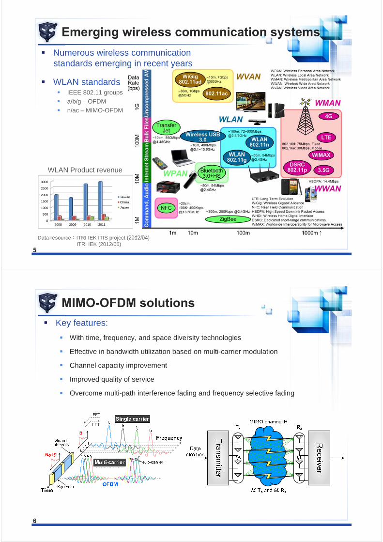
Emerging wireless communication systems
Numerous wireless communicationstandards emerging in recent years
WLAN standards IEEE 802.11 groups
a/b/g – OFDM
n/ac – MIMO-OFDM
Data resource:ITRI IEK ITIS project (2012/04)ITRI IEK (2012/06)
0
500
1000
1500
2000
2500
3000
2008 2009 2010 2011
Taiwan
China
Japan
WLAN Product revenue
5
MIMO-OFDM solutions
Key features:
With time, frequency, and space diversity technologies
Effective in bandwidth utilization based on multi-carrier modulation
Channel capacity improvement
Improved quality of service
Overcome multi-path interference fading and frequency selective fading
6
Page 4
Open Loop MIMO Transceiver Design
Channel state information (CSI) is only known at the receiver known preamble or pilot signals are transmitted and used by the receiver
to determine the channel matrix H.
Linear detection methods: Zero-Forcing (ZF)
Minimum Mean-Squared Error (MMSE)
Nonlinear detection methods: VBLAST (Vertical Bell Labs Layered Space-Time)
Maximum Likelihood (ML)
Sphere Decoding (SD) and Fixed Sphere Decoding (FSD)
7
Close Loop MIMO Transceiver Design
CSI is known at both ends CSI determined at receiver using a channel estimation procedure.
At transmitter, can use either feedback from the receiver or time-division duplexing (TDD) to obtain CSI
Joint MIMO transceiver designs employ pre-coding scheme at the transmitter to facilitate a simple receiver
design
Enables cooperation between the two ends
Performance can be greatly enhanced.
Works well with channel decomposition methods.
8
Page 5
Precoding & joint transceiver designs
The closed-loop MIMO-OFDM systems [25,26]
Information feedback form the receiver to enhance the transmitter design
Perform precoding at the transmitter site to pre-compensate the channel impairments
Linear precoding matrix is obtained from the CSI
Precoding algorithms vary in performance and computing complexity
H
9
Advantages of precoding
Advantages of precoding Suitable for slow fading channel
Improvement of signal-to-noise ratio
Reducing system bit error rate
Multiple independent parallel sub-channels
Effectively reducing computational complexity of signal detection
Obtain the maximal channel capacity
Incurred overheads high computation complexity
Inconsistent computing throughput problem
Considering the bandwidth of precoding
matrix via receiver feedback
Systems performance
10
Page 6
Outline
Overview of precoding techniques
• Linear v.s. non-linear precoding schemes• Generalized triangular decomposition• Uniform channel decomposition• Performance comparison
11
Precoding schemes overview
Applied to the transmitter to create a desired effective channel for the receiver
originally for beamforming operations in multi-antenna communication systems
extended to SDM MIMO systems to pre-compensate the channel impairments
Linear precoding schemes useful in peer to peer communications such as wireless LAN
Aimed at maximizing the channel throughput
decompose a MIMO channel into parallel sub-channels to minimize the interferences between different data streams
Non-linear precoding schemes good at cancelling multi-user interferences
employed mostly in systems supporting multi-cast services
Tomlinson-Harashima Precoding (THP)
12
Page 7
Generalized Triangular Decomposition
Given a channel matrix H, GTD decomposes H = QRP*
P is a linear precoding matrix, Q and P are unitary
R is upper triangular and• Diagonal elements of R satisfy Weyl’s multiplicative majorization conditions
• vector r is multiplicatively majorized by the singular value vector of H
• rii is the i-th largest (in magnitude) diagonal element of R
• the i-th largest singular value of H
• N is the rank of the channel matrixi
1 1 1 1
| | , 1 , | |k k N N
ii i ii ii i i i
r k N r
r λ
Special cases of GTD
QR factorization (QRD)• No precoding ( P = I)
Singular value decomposition (SVD) • R= is a diagonal matrix containing the singular values on the diagonal
• precoding matrix P = V
Schur decomposition • R=U is an upper triangular matrix with diagonal elements as the
eigenvalues of H
• precoding matrix P = Q
Geometric mean decomposition (GMD) • diagonal elements of R are identical
• the geometric mean of positive singular values
14
H = QR
*H = UΣV
*H = QUQ
*H = QRP
1/
1
NN
ii kk
r
Page 8
Singular Value Decomposition
To create multiple parallel sub-channels
sub-channel gains are determined by the singular values
Ill-conditional channel matrix results vastly different SNRs in sub-channels
Need to perform extra water-filling to maximize the channel capacity
extra computing complexity and is inherently capacity lossy due to finite constellation granularity
15
HH = UΛV
Geometric Mean Decomposition
diagonal R for parallel sub-channels
upper triangular R converting the MIMO channel into layered sub-channels to facilitate
successive interference cancellation (SIC) based signal detection.
GMD is the solution to the following maximum problem
Equal diagonal property means the signal decision
boundaries to an SIC scheme are equal in all
dimensions to minimize the bit error rate.
The performance of the GMD scheme can be asymptotically equivalent to that of the maximum likelihood detector (MLD) at high SNR values
16
Page 9
Uniform Channel Decomposition
an extension of the GMD scheme and works in conjunction with a minimum mean square error (MMSE) based equalizer
SVD + water filling precoding
UCD precoding
Virtual channel
Strictly capacity lossless at any SNR
The maximal diversity gain
decompose a MIMO channel into multiple subchannels with desired channel capacities
Need to perform SVD, GMD, MMSE, water-filling, etc.
Most computationally expensive
17
2* 1/2
2 2, , ( ) , z
kk x
H = UΛV P = VΦ
1/2 * *, , with and L N L N P = VΦ Ω Ω Ω Ω I1/2 *G HP UΛΦ Ω
UCD-VBLAST scheme
Consist of a linear precoder and the MMSE-VBLAST detector
Channel decomposition flow SVDWater-filling MMSE GMD obtain preocding matrix
1
2JF = VΦ P
aa J=α L
G
HFG = Q R
I
1
2Φ
1
2F = VΦ
*H = UΛV
1
2aF = VΦ P
*a a a aH = Q R P
aa G aG = Q R
Reduce the computational complexity
• Compare any matrix and augmented Amatrix with SVD
• Applying GMD to
• Reduction of unitary matrices updatingand augmented matrix with GMD
* *, A A A B B B
BA U V B U V
I
2, , , 1,...,A i B i i N
18
Page 10
Performance comparison
Precoding provides significant BER improvements
UCD has the best performance but also the highest computing complexity
GMD seems to achieve a good balance between the BER improvement and the computing overhead
19
Outline
Problem statement and proposed work
• conventional GMD computing scheme• problem statement• proposed work
20
Page 11
SVD-based GMD scheme
Perform N × N SVD followed by N × N GMD
Algorithm:
First, SVD
Second, permutation
Final, converting singular value to geometric mean
t r
s s
x y
HH
PP
*H UΛV 411 22 33 44
1, 1 1, 1(r and r ) or (r and r )kk k k kk k k ( ) ( )
k k
k kR R
1 2 1
2 1 2
cδ sδ δ 0 c s x1
sδ cδ 0 δ s c 0 y
2 222
2 21 2
δc and s 1 c
δ δ
Complex-valued 4 × 4 GMD example
21
Convergence problem in SVD
Zero-shift based SVD The diagonal above the main diagonal can be zero via iterative operations
Jacobi-based SVD Off-diagonal can be zero via iterative operations
: Non-zero elements
: Zero elements
: Computation elements
: Perform a sweep result
: Perform a sweep result of singular value
22
Page 12
Problem Statement
Observations Precoding scheme computing complexity with an order of at least
Require tremendous computing power, hardwired solution is a must
Convergence problem in SVD computation, adverse to constant throughput implementation
Problem statement
Devise a new GMD computing scheme free of the convergence problem
Low computing complexity
Hardware sharing between the precoding and signal detection
Features of the proposed scheme
No SVD pre-processing, bidiagonalization is used instead
Constant throughput, free of convergence problem
A divide-and-conquer scheme for any matrix sizes
Shared computing kernels with QR-BLAST signal detector
Application to arbitrary matrix size, most efficient with matrix size of power of 2
23
3( )O N
Proposed GMD computing scheme
Investigated topics
• Multi-function• Constant throughput• Low complexity• High data rate
ChipImplementation
CircuitDesign
Mapping
Algorithm • Divide-and-conquer• Proposed scheme
• DG, SFG• Multi-projection• Pipeline, parallelism
• Bottom-up design• Modules design• Circuit design techniques• Integration
• TSMC 90nm process• Chip design• Various simulations
The chip of 4 × 4 QRD / GMD joint design
24
Page 13
Outline
Proposed efficient GMD computing scheme
• Mathematical Formulation• Basic 2 × 2 sub-matrix computing schemes• Divide-and-conquer based GMD scheme• Performance and complexity analysis
25
Mathematical Formulation
Mathematical models
Dividing the bidiagonal matrix R into N / 2 sub-matrix, and performing log2N stage for each 2 × 2 sub-matrix.
Using complex-valued to real-valued conversion
( ) ,
ˆ ˆ( ) ,
H
H
y Hx n
QRP x n x Ps
QRP Ps n Hs n H QR SIC
ˆ,
( ) ,H H H H H
y Hs n H H
Q y Q QR s Q n, y Q y n Q n
y Rs n s
Precoding operation- GMD
Signal detection- QR-SIC
N
N
2N
R
R
I
I
R
I
s s
x y
H
PPH
2log N
R/ 2N
Re - Im ; Im Re( ) H H H H H H T
26
Page 14
Basic 2 × 2 sub-matrix computing schemes
Four basic operations
Complex-valued Givens rotation• First, convert it to the real-valued
by cancelling the imaginary parts
• Second, nullify the lower entry
1
2
' 0
' 0
j
j
x xe
y ye
3 3
3 3
'' cos sin '
0 sin cos '
x x
y
2 × 2 SVD operation• Matrix diagonalization
• δi and δi+1 are singular value and both positive
• Without convergence problem
1
1
cos sin 0cos sina b
sin cos 0sin cos0 dil l ir r
l il ir r
2 × 2 GMD operation• Matrix trangularization
• The equal geometric mean of diagonal δi and δi+1
• Always satisfying the permutation condition
,
,
,
,1
cos sin 0 cos sin
0sin cos 0 sin cosk ul l i r r
k ul l
k u
kr ui r
x
2 × 2 SWAP operation• swapping diagonal entry
1 1 2 2
1 1 2 2
sin cos sin cosa b d b
cos sin cos sin0 d 0 a
Applying to proposed GMD scheme
All operations can be implemented using the CORDIC
27
Proposed GMD algorithm
Step 1: Performing the matrix bidaigonalization scheme Nullification by a series of row-wise and column-wise Givens rotation
Step 2: Low-complexity equal diagonal conversion scheme Reshuffling the diagonal elements
Performing the divide-and-conquer GMD
22 1 1 1
, ,0 0
N N
r i c ii i
B H R R
a a or a b a 0
b 0
c s c s
s c s c
28
Page 15
Matrix bidiagonalization scheme
Performing a series of unitary matrix decomposition Example of the 4 × 4 channel matrix
k is in charge of nullifying the off-diagonal elements on kth column and kth row
i1, i2 are performed the column nullification by row-wise Givens rotations
j1, j2 are the row nullification by column-wise Givens rotations
=1, =1 to 4 =1, =3 to 1 =1, =2 to 4 =1, =3 to 2 =2, =2 to 4 =2, =3 to 2 =2, =3 to 4
=2, =3 =3, =3 to 4 =3, =3 =3, =4 =4, =4 Final result
H
Real-valued elements
zero elements
Bidiagonal elements
Elements to be updated
Elements to be nullified
29
Equal diagonal conversion scheme (1)
The geometric mean of a set of N singular values can be computed in a divide-and conquer manner
“Divide” – divide into log2N stages
– start with a group size of 2
– end with a group size of N
“Conquer” – diagonal element reshuffling
– 2 × 2 SVD
– 2 × 2 GMD
Diagonal element reshuffling The goal is to end up with a diagonal Featuring
alternate geometric mean values
2 21 2 1 2 2 1
4 4 4 41 4 4 1 2 2 1 3 4 3 4 1
1 2 3 4 3 2 1
N NNN N N N
N N N NN N N N N N N
N N N N
11r
22r
33r
44r
55r
66r
77r
88r
30
Page 16
Equal diagonal conversion scheme (2)
Example of 8 × 8 bidiagonal matrix
R
1 2 3 4 5 6 7 8 41 2 3 4 4
5 6 7 8 81 2 3 8
31
Equal diagonal conversion scheme (3)
Pseudo code of proposed scheme First step
• Parallel loop structure
• Operation: 2 × 2 SVD, GMD
• Performing log2N stages
Second step
• Nested loop structure
• Operation: 2 × 2 SWAP
• Performing log2N-1 stages
201.
02.
03.
04.
05.
06.
1 log
1 -1 ( 2)
SVD2X2( , );
GMD2X2( , );
k N
i N i i
i
i
For to do
Parfor to do
R
R
End
2
1
1
1
2
2
07.
08.
09.
10.
11.
log
2 ; 2 1;
1
2 2 1
1
is odd
k k
k
k N
W L
j N W
m j
j L
j
If then
Parfor to do
For to
If then
2
3 2
3
12.
13.
14.
15.
SWAP2X2( , );
1
1 ( 1) / 2
- 2 ;
m
j
j j
p m j
R
If then
Parfor to do
3
216.
17.
18.
19.
2 ;
is even
1; -1;
q m j
j
p p q q
If then
End
20.
21.
22.
23.
24.
25.
SWAP2X2( , ); SWAP2X2( , );
p pR R
End
End
End
End
End
End
2 × 2 SVD + GMD
Reshuffle
32
Page 17
Performance evaluation
MIMO size: 4 × 4 / 6 × 6
OFDM size: 64 (16-point CP, 8-point Null)
Modulation: 64-QAM
Channel delay spread (r.m.s): 11 taps
GMD precoding and QR-BLAST signal detector
Precoding matrix at transmitter via perfect feadback
Zero-shift: N / 2 sweep; Jacobi: log2N sweep
0 5 10 15 20 2510
-3
10-2
10-1
100
4x4 MIMO-OFDM 64-QAM with QR-BLAST
SNR(db)
Sym
bole
Err
or R
ate
GMD-SVD MATLAB
Proposed schemeGMD-SVD(zero-shift) sweep:1
GMD-SVD(zero-shift) sweep:2
GMD-SVD(zero-shift) sweep:3
GMD-SVD(zero-shift) sweep:4
GMD-SVD (Jacobi) sweep:2GMD-SVD (Jacobi) sweep:3
GMD-SVD (Jacobi) sweep:4
0 5 10 15 20 2510
-5
10-4
10-3
10-2
10-1
100
6x6 MIMO-OFDM 64-QAM with QR-BLAST
SNR(db)
Sym
bole
Err
or R
ate
GMD-SVD MATLAB
Proposed schemeGMD-SVD(zeor-shift) sweep:1
GMD-SVD(zeor-shift) sweep:2
GMD-SVD(zeor-shift) sweep:3
GMD-SVD(zeor-shift) sweep:4
GMD-SVD(Jabobi) sweep:2GMD-SVD(Jabobi) sweep:3
GMD-SVD(Jabobi) sweep:4
33
Computational complexity analysis
Take the convergence factor of SVD operations into consideration Zero-shift: N / 2 sweep numbers
Jacobi: log2N sweep numbers
Analysis of matrix decomposition and precoding updating Antenna size: 4, 8, 16
34
Page 18
Outline
Algorithm mapping and architecture design
• Combined GMD / QRD design specification• Algorithm mapping• Architecture design
35
Combined GMD / QRD design specification
Combined GMD design for precoding and QRD design for signal detection
Subject to 802.11ac VHT PHY standard
Four VHT-LTF are transmitted at 16 s with long guard interval
Need to perform 468 complex-valued matrix decompositions
Assume 1 LTF time slots are allocated for GMD computations
time span per decomposition = 4 s / 468 = 8.548 ns (117 M decompositions/sec)
Set 4 clocks as the initiation interval for each new decomposition, equivalent to 468MHz
Employ three parallel modules, each has a operation frequency: 160 MHz
Parameter Value Parameter Value
Channel bandwidth 160 MHz FFT size (N) 512
Spatial streams (NSS) 4 Data tones (NSD) 468
MCSs 6 Pilot tones (NSP) 16
Modulation 64-QAM Null tones 28
Coding rate (R) 3/4 IFFT/FFT (TFFT) 3.2 s
Technology MIMO/SDM Short guard interval (TGIS) 0.4 s
Data rate 2340.0 Mbps Long guard interval (TGIL) 0.8 s
36
Page 19
Dependence Graph of the GMD scheme
Each DG node is the row-wise or column-wise
Givens rotation
11
4
4
3
3
3
3 4
2
1
33bk = 3
112b
3 4
3
4
2
2
3
2
2 3 4
i
li
l
22b= 2
j2l
j
23b
l
11b
34b
44b
D&C GMDStage 1
D&C GMDStage 2
Column nullification
Row nullification 37
Fully parallel architecture mapping
Fully parallel mapping from DG to SFG Fully parallel to meet the throughput requirement
3-dimension: j, k are data propagation; i is angle of rotation
D is global delay of data propagation path
CORDICs replace the Givens rotations 3D DG 4D DG: l-dimension: the CORDICs iteration
Further SFG mapping by multi-projection Reduce the dimension by 1, local delay
Projection vector d and Scheduling vector s =
Each edge delay
Scheduling constraints
[0 0 0 1]t
D D ts e
J t
D ( 1) tM s d
D D = ∙τ
D Dτ
τ
τ
τ
τ τ
: Givens Generation(GG)
: Givens Rotation(GR)
38
Page 20
SFG mapping result
CORDIC-based architecture
High parallelism
The number of CORDIC: 174
39
Preliminary architecture designfor 4 × 4 QRD / GMD
Multi-function Signal detection mode (QRD)
Precoding mode (GMD)
Modules Triangularization, Bidiagonalization
2 × 2 SVD, GMD, SWAP
Off-diagonal updating, Precoding generation, Vector updating
y
Key features: using novel GMD scheme
fully-parallel architecture
low complexity
constant throughput
CORDIC-based design
40
Page 21
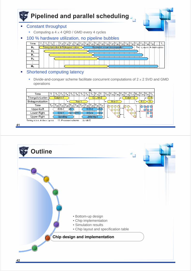
Pipelined and parallel scheduling
Constant throughput Computing a 4 × 4 QRD / GMD every 4 cycles
100 % hardware utilization, no pipeline bubbles
Shortened computing latency
Divide-and-conquer scheme facilitate concurrent computations of 2 × 2 SVD and GMD operations
††
††
41
Outline
Chip design and implementation
• Bottom-up design• Chip implementation• Simulation results• Chip layout and specification table
42
Page 22
Bottom-up design flow
Modules design:
2 × 2 SVD operationPre-processing module
• Triangularization• Bidiagonalization• Simplified SVD scheme
2 × 2 GMD operation
2 × 2 SWAP operationOther matrix updating modules
• Off-diagonal updating• Precoding generation• Received vector updating
GMDIntegration• Hardware sharing• CORDIC Tree• Retiming• Multi-clock domain
43
CORDIC module design
Performing the iterative micro-rotations θ = θ1 + θ2 + θ3 + θ4 + …
Only perform addition, subtraction, and shifter
Need to multiply scaling factor K
Three types of CORDIC in 4 × 4 QRD / GMD design
1
1
cos sin
sin cosi i
i i
x x
y y
11
1 0
cos sin
sin cos
ni i i i
i i i ii
x x
y y
11
01
1 2
2 1
ini ii
iii ii
x xK
y y
>> >>
>> >>
Iteration:0, 2, 4, 6
Givens Generation(GG)
0x
0y
nx
0
Iteration:1, 3, 5, 7
σi
>> >>
>> >>
Givens Rotation(GR)
0x
0y
nx
ny
NullificationNullification UpdatingUpdating
1
K 0cos z
0sin z
Calculate angle
Calculate angle
44
Page 23
GG GG GG GG
GG GG
GG
GG GG GG
GG
GG
Q Mode P Mode
H
H
(16 12-bit)16
16
1713
9
61
1
GG
GR GR
GG GG
GG
GG GG
GG
GG
update Three dimension CORDIC tree
Based GG: 4 componentsEI GR: GG-1ER GR: 2(GG-1)
GG GG GG
GG
GG
update
Based GG: 3 componentsEI GR: GGER GR: 2GG
Q Mode P Mode
Hardware sharing
1 data / 4 clocks
1 data / 1 clocks
Pre-processing module design
Functions: Triangularization (Q mode), 60.38%
Bidiagonalization (P mode), 36.79%
Simplified SVD scheme, 2.83%
No fill-ins occur during the alternatenullification process
Hardware reusing of Triangularizationfor signal detection mode
Hardware sharing of constantmultiplier for scaling factor
CORDICCORDIC
Constant multiplierConstant multiplier
Interconnection bufferInterconnection buffer
37.65%
73.12%
43.8%
45
2 × 2 SVD operation design
3 modules are needed in 4 × 4 design
Low complexity design:
dirs dird dirl dirr
-1 -1 0 -1
-1 +1 -1 0
+1 -1 +1 0
+1 +1 0 +1
1
1
cos sin 0cos sina b
sin cos 0sin cos0 dil l ir r
l il ir r
1tans r l
b
d a
1tand r l
b
d a
1 1tan (b / d a) tan ( b / d a)θ
2l
1 1tan (b / d a) tan ( b / d a)θ
2r
0
0
ad b ad b
a
bd
0 0
0
1δ
2δ
To reduce angle calculation for each CORDIC module
CORDICCORDIC
Other computationOther computation
12.5%
33.3%
46
Page 24
2 × 2 GMD operation design
4 modules are needed in 4 × 4 design Using the CORDIC computing features to simplify the computational
complexity of rotation angle
To further simplify with sum of the rotation angle of 90°
CORDICCORDIC
Other computationOther computation
LatencyLatency
85.71%
55.56%
6 clock cycles
Inv.
Updating the 2 2 matrix
Calculation of direction
1δ
2δ
x
σ
dir
1 1 1 2 2
1 1 2 2 2
cosθ sinθ δ 0 cosθ sinθ σ x
sinθ cosθ 0 δ sinθ cosθ 0 σ
1 21
1
δθ tan
δ
1 12
2
δθ tan
δ
,
,
,
,1
cos sin 0 cos sin
0sin cos 0 sin cosk ul l i r r
k ul l
k u
kr ui r
x
11tan sin cosl i r i r
1 2 2 2 2, , 1tanr i k u k u i
Conventional algorithm
1 2 2 11 1 1 2 2
1 1 2 2 2 1 2
δ δ δ δcosθ sinθ δ 0 cosθ sinθ
sinθ cosθ 0 δ sinθ cosθ 0 δ δ
47
2 × 2 SWAP operation design
Only 1 module is needed in 4 × 4 design Reduce the complex calculation of the angle
CORDICCORDIC
Other computationOther computation 33.33%
50.00%
z y-x θr θl
+ + + +
+ - - -
- + - -
- - + +
11
11
0, tan ( / )
0, tan ( / )r
r
z y x
z y x
12
12
θ 0, θ tan ( z / y x)
θ 0, θ tan (z / y x)l
l
1 1 2 2
1 1 2 2
sin cos sin cos
cos sin cos sin0 0
x z y z
y x
1tanr l
z
y x
1tanr l
z
y x
1 r l
2 l r
Proposed 2 × 2 SWAP algorithm
Without any computation on hardware implementation Considering elements updating
Only need one exclusive OR gate to obtain angle of direction
48
Page 25
Summary circuit design techniques
1. Hardware sharing Constant multipliers are shared for each CORDIC
Multipliers are shared for the precoding module
Hardware reusing on the trangularization module
2. Binary tree nullification scheme To shorten the computing latency
3. Retiming design To reduce the data buffer
i.e. precoding generation, off-diagonal updating
4. Multi-clock domain design To reduce the data buffer
i.e. data output buffer, direction buffer
1x
1y
2x
3x
4x
2y
3y
4y
1x
1y
2x3x4x
2y3y4y
MU
XM
UX
Hardware sharingHardware sharing
RetimingRetiming
Binary treeBinary tree
49
Chip implementation issues
Chip I/O port To meet chip data bandwidth
Selection of data output types:• upper triangular matrix R• precoding matrix P• received vector Y
Clock gating design To reduce power consumption
Using latches to avoid glitch
Precoding mode: 190 mW
Signal detection mode: 112 mW
Scan chain for chip measurement Scan chain length: 15049 D-FF
Fault coverage: 99.9%
Generating test pattern form ATPG: 244
Extra hardware cost: 30 k gates
OUT_S
OUT_S
CH1_RCH1_PCH1_Y
CH2_RCH2_PCH2_Y
DATA_CHA
DATA_CHB
14
14
15
13
15
15
13
15
2
2
Latch
Data output
Data input
Clock gating
Scan chain50
Page 26
Simulation results (1)
Effects of CORDIC iteration Latency
Precision
Word length
SER 10-3 lose 0.4 dB when CORDIC iteration 8 times
11-bit fraction precision are close to floating-point operation
0 5 10 15 20 2510
-4
10-3
10-2
10-1
100
101
SNR (dB)
Sym
bol E
rror
Rat
e (S
ER
)
4 x 4 MIMO-OFDM by combining GMD with QR-BLASTcomparing of different CORDIC iteration
Proposed 4 x 4 GMD scheme (software)CORDIC iteration: 1
CORDIC iteration: 2
CORDIC iteration: 3
CORDIC iteration: 4CORDIC iteration: 5
0 5 10 15 20 2510
-4
10-3
10-2
10-1
100
101
SNR (dB)
Sym
bol E
rror
Rat
e (S
ER
)
4 x 4 MIMO-OFDM by combining GMD with QR-BLASTanalysis of fixed-point
Proposed 4 x 4 GMD scheme(hardware, floating, 4-iteration)Bits of fraction: 1-bit
Bits of fraction: 2-bit
Bits of fraction: 3-bitBits of fraction: 4-bit
Bits of fraction: 5-bit
Bits of fraction: 6-bit
Bits of fraction: 7-bitBits of fraction: 8-bit
Bits of fraction: 9-bit
Bits of fraction: 10-bitBits of fraction: 11-bit
Bits of fraction: 12-bit
Bits of fraction: 13-bitBits of fraction: 14-bit
51
Simulation results (2)
Implementation lost: 0.5 dB
0 5 10 15 20 2510
-4
10-3
10-2
10-1
100
101
SNR (dB)
Sym
bol E
rror
Rat
e (S
ER
)
4 x 4 MIMO-OFDM by combining GMD with QR-BLAST
Traditional 4 x 4 GMD schemeProposed 4 x 4 GMD scheme (software)
Proposed 4 x 4 GMD scheme(hardware, fixed-point, 4-iteration, 11-bit of fraction)
A B C
C
GMD-1 GMD-2 GMD-3 GMD-4 GMD-5
A: Input data buffering• 16 clock cycles• 4 × 4 complex-valued channel matrix
generation per 4 clock cycles
B: 4 × 4 QRD / GMD computing• QRD latency: 54 clock cycles• GMD latency: 128 clock cycles
C: Results of constant throughput
52
Page 27
Chip layout and specification table
Chip layout Specification table
Hardware utilization
53
Outline
Conclusion
54
Page 28
Conclusion
Overview of precoding schemes Generalized triangular decomposition
SVD vs. GMD vs. UCD
New GMD computing scheme Present and efficient GMD computing scheme for the precoding matrix calculation
Non-iterative and low-complexity process
Free of the numerical convergence
Facilitate a constant throughput computation
Application to arbitrary matrix size, most efficient with matrix size of power of 2
Chip design Present a multi-function QRD/GMD chip design for closed-loop MIMO-OFDM
communication systems
Support the precoding mode and the signal detection mode
Using CORDIC and GMD computing features to further simplify hardware utilization
Various circuit design techniques are used in this chip to reduce cost
High operation frequency and high data rate
55