DESIGN AND INSTRUMENTATION OF THE STRUCTURAL PAVEMENT ... Reports/04-01 Design and... · DESIGN AND...

NCAT Report 04-01

DESIGN AND INSTRUMENTATION OF THE STRUCTURAL PAVEMENT EXPERIMENT AT THE NCAT TEST TRACK By David H. Timm Angela L. Priest Thomas V. McEwen

April 2004

277 Technology Parkway Auburn, AL 36830

DESIGN AND INSTRUMENTATION OF THE STRUCTURAL

PAVEMENT EXPERIMENT AT THE NCAT TEST TRACK

By:

David H. Timm Assistant Professor of Civil Engineering National Center for Asphalt Technology Auburn University, Auburn, Alabama

Angela L. Priest

Research Assistant National Center for Asphalt Technology Auburn University, Auburn, Alabama

Thomas V. McEwen

Instrumentation Consultant

NCAT Report 04-01

April 2004

- i -

DISCLAIMER

The contents of this report reflect the views of the authors who are responsible for the facts and accuracy of the data presented herein. The contents do not necessarily reflect the official views or policies of the National Center for Asphalt Technology of Auburn University. This report does not constitute a standard, specification, or regulation.

ACKNOWLEDGEMENTS

The authors wish to thank the Alabama Department of Transportation, the Indiana Department of Transportation and the Federal Highway Administration for their support and cooperation of this research.

- ii -

TABLE OF CONTENTS Page CHAPTER 1 – INTRODUCTION ...............................................................................................1 Background..........................................................................................................................1 Objectives ............................................................................................................................4 Scope ..................................................................................................................................4 Organization of Report ........................................................................................................4 CHAPTER 2 – THICKNESS DESIGN OF TEST SECTIONS ................................................5 Introduction..........................................................................................................................5 Experimental Design............................................................................................................5 Structural Design .................................................................................................................6 Test Section Layout .............................................................................................................8 CHAPTER 3 – INSTRUMENTATION: PRE-INSTALLATION ...........................................9 Introduction..........................................................................................................................9 Sensor Selection...................................................................................................................9 Asphalt Strain Gauges..............................................................................................9 Earth Pressure Cells ...............................................................................................10 Subgrade Moisture Probes .....................................................................................11 Temperature Profiles..............................................................................................12 Additional Instrumentation ....................................................................................12 Soil Compression Gauge............................................................................13 Miniature Pressure Cell..............................................................................13 Preinstallation Efforts ........................................................................................................14 Asphalt Strain Gauges............................................................................................14 Earth Pressure Cells ...............................................................................................14 Subgrade Moisture Probes .................................................................................................16 Additional Instrumentation ....................................................................................18 Data Acquisition ................................................................................................................19 Slow Speed Data Acquisition ................................................................................19 High Speed Data Acquisition.................................................................................22 High Speed Sensor Layout and Labeling...........................................................................22 Gauge Layout.........................................................................................................23 Gauge Labeling......................................................................................................32 Temperature and Moisture Gauge Positioning ..................................................................34 Summary ....................................................................................................................35 CHAPTER 4 – SENSOR INSTALLATION .............................................................................36 Introduction ....................................................................................................................36 Subgrade Moisture Probes and Earth Pressure Cells.........................................................36 TDR Moisture Probes ............................................................................................36 Subgrade Earth Pressure Cells ...............................................................................38 Granular Base Layer Construction.........................................................................40 Base Pressure and Button Cells, Asphalt Strain and Compression Gauges ......................42 Gauge Marking and Excavation.............................................................................42 Gauge Installation ..................................................................................................45 Base Earth Pressure Cells and Button Cell ................................................45

- iii -

Page Asphalt Strain Gauges................................................................................46 Vertical Compression Gauges....................................................................51 Temperature Probes ...........................................................................................................52 Gauge Monitoring During Construction and Survivability ...............................................53 Summary ....................................................................................................................64 CHAPTER 5 – SUMMARY, CONCLUSIONS AND RECOMMENDATIONS...................65 REFERENCES.............................................................................................................................66 APPENDIX A – INSTRUMENTATION DATA SHEETS ......................................................68 APPENDIX B – HIGH SPEED DATA ACQUISITION – CHANNEL ASSIGNMENTS ....................................................................................................................73

- iv -

LIST OF TABLES Table Page Table 2.1 Structural Design Inputs .................................................................................................6 Table 2.2 2003 Test Track Structural Sections – Preliminary Design............................................7 Table 2.3 2003 Test Track Structural Sections – Recommended Design.......................................8 Table 3.1 TDR Probe Calibration Coefficients.............................................................................19 Table 3.2 Wheelpath Locations ....................................................................................................25 Table 4.1 Asphalt Strain Gauge and Earth Pressure Cell Survivability .......................................54 Table 4.2 Section N1 Survivability...............................................................................................55 Table 4.3 Section N2 Survivability...............................................................................................56 Table 4.4 Section N3 Survivability...............................................................................................57 Table 4.5 Section N4 Survivability...............................................................................................58 Table 4.6 Section N5 Survivability...............................................................................................59 Table 4.7 Section N6 Survivability...............................................................................................60 Table 4.8 Section N7 Survivability...............................................................................................61 Table 4.9 Section N8 Survivability...............................................................................................62

- v -

LIST OF FIGURES Figure Page Figure 1.1 Typical M-E Design Flowchart .....................................................................................2 Figure 2.1 Existing Test Track Cross Section (after Jess, 2004). ...................................................6 Figure 2.2 Final Design and Section Layout ..................................................................................8 Figure 3.1 CTL Asphalt Strain Gauge ..........................................................................................10 Figure 3.2 Geokon Earth Pressure Cell.........................................................................................11 Figure 3.3 Geokon Earth Pressure Cell at the Test Track.............................................................11 Figure 3.4 TDR Moisture Probe ...................................................................................................12 Figure 3.5 Thermistor Bundle for Measuring In Situ Temperature..............................................12 Figure 3.6 Vertical Compression Gauge.......................................................................................13 Figure 3.7 Tokyo Sokki Pressure Cell ..........................................................................................13 Figure 3.8 Strain Gauge Functionality Checks .............................................................................14 Figure 3.9 Earth Pressure Cell Calibration at the Aquatic Center ................................................15 Figure 3.10 Summary of Earth Pressure Cell Calibration Data (14.5 psi gauges) .......................15 Figure 3.11 Summary of Earth Pressure Cell Calibration Data (36.3 psi gauges) .......................16 Figure 3.12 Calibration of Moisture Probes .................................................................................17 Figure 3.13 TDR Calibration Data – All Gauges .........................................................................18 Figure 3.14 Roadside Data Collection System .............................................................................21 Figure 3.15 50-pin Connector .......................................................................................................21 Figure 3.16 Dataq DI-510-32 High Speed Data Acquisition System...........................................23 Figure 3.17 Zone of Influence Evaluation ....................................................................................24 Figure 3.18 Wheelpath Markings for Cells N1 and N8 ................................................................25 Figure 3.19 Sections N1, N3, N4, N5 High Speed Sensor Layout ...............................................27 Figure 3.20 Section N2 High Speed Sensor Layout .....................................................................28 Figure 3.21 Section N6 High Speed Sensor Layout .....................................................................29 Figure 3.22 Section N7 High Speed Sensor Layout .....................................................................30 Figure 3.23 Section N8 High Speed Sensor Layout .....................................................................31 Figure 3.24 3D Schematic of Common High Speed Gauge Arrangement ...................................32 Figure 3.25 N1 High Speed Sensor Identification (not to scale) .................................................33 Figure 3.26 Gauge Labeling Using Heat Gun and Shrink Tubing ...............................................34 Figure 4.1 TDR and Earth Pressure Cell Cavities and Trenches..................................................37 Figure 4.2 Compacting TDR Cavity and Backfilled Cable Trenches ..........................................37 Figure 4.3 Complete TDR Installation..........................................................................................38 Figure 4.4 Leveling Subgrade Earth Pressure Cell .......................................................................39 Figure 4.5 Complete Earth Pressure Cell Installation...................................................................40 Figure 4.6 Hand Placement of Granular Base Material ................................................................41 Figure 4.7 Base Construction and Gauge Monitoring ..................................................................42 Figure 4.8 Establishing Center of Gauge Array and ASG Locations ...........................................43 Figure 4.9 Gauge Location Markings for Cell N3........................................................................43 Figure 4.10 Cell N8 Excavation for ASG’s and Earth Pressure Cells..........................................44 Figure 4.11 Placement of Button Cell in Section N6.....................................................................45 Figure 4.12 Approximate Placement of ASG’s ............................................................................46 Figure 4.13 ASG with Cable Tie Missing from Axial Bar ...........................................................47 Figure 4.14 ASG with Additional Cable Ties...............................................................................47

- vi -

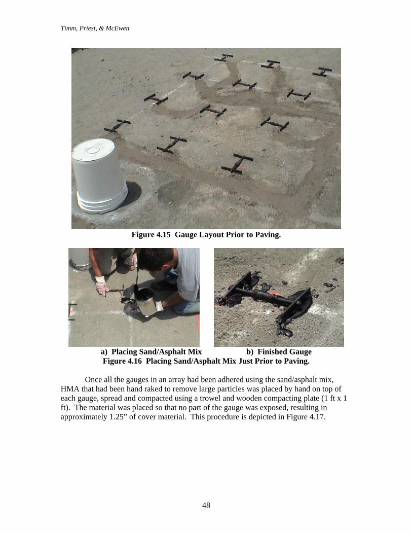
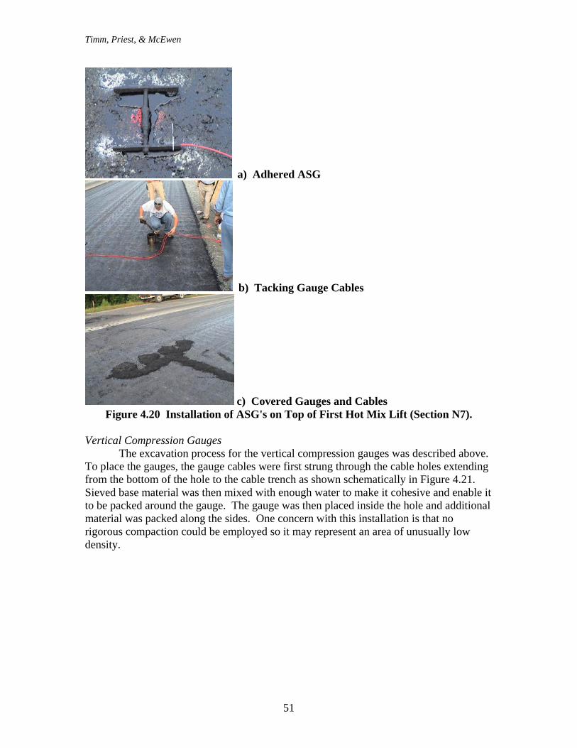
Figure Page Figure 4.15 Gauge Layout Prior to Paving ...................................................................................48 Figure 4.16 Placing Sand/Asphalt Mix Just Prior to Paving ........................................................48 Figure 4.17 Placing Cover Material on ASG’s.............................................................................49 Figure 4.18 Paver Straddling Gauge Array...................................................................................50 Figure 4.19 Monitoring Gauges During Construction..................................................................50 Figure 4.20 Installation of ASG’s on Top of First Hot Mix Lift (Section N7).............................51 Figure 4.21 Vertical Compression Gauge Installation..................................................................52 Figure 4.22 Completed Temperature Probe Installation...............................................................53 Figure 4.23 An Example of a Functioning Sensor Under Traffic.................................................63 Figure 4.24 An Example of a Sensor Behaving Erratically Under Traffic...................................63 Figure 4.25 An Example of a Sensor Exhibiting Excessive Noise...............................................64 Figure 4.26 An Example of a Sensor Not Responding Under Load.............................................64

Timm, Priest, & McEwen

1

DESIGN AND INSTRUMENTATION OF THE STRUCTURAL PAVEMENT EXPERIMENT AT THE NCAT TEST TRACK

David H. Timm, Angela L. Priest, and Thomas V. McEwen

CHAPTER 1 - INTRODUCTION

BACKGROUND For over fifty years, test roads have been an integral part of the advancement of pavement research and engineering. Beginning with the early Maryland Road Test (HRB, 1945), continuing with the AASHO Road Test (HRB, 1962), the WESTRACK experiment (Epps, et al., 1998), the Minnesota Road Research Project (Mn/DOT, 2003; Mn/DOT 1990), the Virginia Smart Road (Loulizi, et al., 2001; Smart Road, 2003) and the NCAT Test Track (Brown, et al., 2002), much knowledge regarding pavement design, performance and construction has been gained. The foremost among these test roads was the AASHO Road Test conducted in Ottowa, Illinois from 1958 to 1960. The data gathered during this testing cycle form the basis of the current AASHTO Design Guide for Pavement Structures (AASHTO, 1993). The current design guide, though widely used in the United States and around the world, is limited to the original conditions at the road test and is strictly empirical in nature. The conditions at the road test included one environmental condition, a limited number of axle weights, tire pressures and axle configurations and only 1.1 million axle load repetitions from which empirical design equations were developed. Today, it is common to design pavements for tens of millions of truck passes, including widely varying climatic conditions, highly variable axle weights, tire pressures and different axle configurations. Consequently, the empirical design equations may no longer be valid. Due to the limited nature of the original AASHO Road Test, the pavement engineering community at large has recognized a pressing need to move beyond empirically-based design and analysis toward mechanistic-empirically (M-E) based procedures. These types of procedures rely on predicting pavement response under load (i.e., stress, strain, deflection) and empirically relating these to field performance. The result is a more robust analysis and design approach that is applicable over a much wider range of conditions and can adapt to new materials, traffic and other technologies. A typical design flowchart for M-E design is shown in Figure 1. One such example of an M-E based procedure is the forthcoming AASHTO Design Guide for Pavement structures under development by NCHRP Project 1-37A (NCHRP, 2003). The outcome of 1-37A is to have a fully-functional M-E based design system to replace the current AASHTO Guide (AASHTO, 1993). While 1-37A is under development, other state agencies have been working on or have in place M-E based design systems. These include, but are not limited to: Washington State DOT, Minnesota DOT, Illinois DOT and Idaho DOT.


2

Figure 1.1. Typical M-E Design Flowchart.

Mechanistic Model

Design Inputs - Layer thicknesses - Material Properties - Load Configurations- Load Repetitions

Pavement Strain

Transfer Functions 21

1

k

tf kN ⎟⎟

⎠

⎞⎜⎜⎝

⎛=

ε (fatigue)

413

k

vr kN ⎟⎟

⎠

⎞⎜⎜⎝

⎛=

ε (rutting)

Nf, NrMiner’s Hypothesis

∑∑= =

=m

i

k

j ij

ij

Nn

D1 1

i = season

j = load configuration n = number of repetitions

under condition i,j

Df (fatigue)Dr (rutting)

Df > 1? Df << 1? Dr > 1?

Dr << 1?

Final Design Thicknesses

Yes

No


3

Central to the development of any M-E design system, including those listed above, is a sound pavement performance data set on which to base the empirical relationships between pavement response and pavement performance. Also known as transfer functions, these relationships provide the essential link between the mechanistic and empirical sides of modern pavement design. One such set of equations, to predict the number of load cycles until fatigue failure in asphalt concrete and structural rutting, respectively, have the common form:

211

k

tf kN ⎟⎟

⎠

⎞⎜⎜⎝

⎛=

ε (1.1)

413

k

vr kN ⎟⎟

⎠

⎞⎜⎜⎝

⎛=

ε (1.2)

where: Nf = number of load repetitions until fatigue failure Nr = number of load repetitions until rutting failure εt = maximum tensile strain at the bottom of the asphalt concrete layer εv = maximum compressive strain at the top of the subgrade k1, k2, k3, k4 = empirically derived constants While the strains are mechanistically determined through a load-response model, the empirical constants must be determined from laboratory or field performance data. If determined in the lab, a shift factor must often be applied to obtain accurate estimates of field performance (Newcomb et al., 1983). Alternatively, they can be derived directly from field data and no shift factors are required (Timm and Newcomb, 2003). In either case, field data are required for accurate performance predictions. An additional problem to overcome regarding transfer functions is that they tend to be somewhat mix-specific. For example, a low stiffness mixture may be more fatigue resistant (resulting in different k1 and k2) than a stiffer mix (e.g., Huang, 2004). Therefore, there is a need to evaluate a variety of mixtures and pavement sections to determine the empirical constants. While much research has been done to determine these values, there has been little effort to study the effect of polymer modification on fatigue performance in the field. Therefore, there is a need to examine what impact, if any, polymer modification may have on pavement response and/or fatigue performance. Another important consideration in M-E design and analysis is the accuracy of the load response model in predicting pavement response under moving loads. Historically, analyses have been limited to static loads resting on layered elastic systems. Generally speaking, these approaches have proven reasonably accurate for design purposes (e.g., Chadbourn et al., 1997). However, there is a need to further validate the load response models, particularly in light of dynamic pavement response. In other words, what is the pavement response under dynamic loading, particularly as the pavement deteriorates and becomes more rough? Given the paradigm shift from empirically-based design analysis toward M-E there is a need to address the issues discussed above. Test roads such as the Minnesota Road Research Project and the Virginia Smart Road have instrumented pavement


4

sections with pavement response devices such as strain gauges and pressure cells to address the needs stipulated above. While they have begun to address some of the important M-E issues, there is certainly a need for further investigation, particularly in light of varying material types, varying material properties and climatic conditions. To that end, a structural experiment at the NCAT test track was warranted to advance M-E design and analysis. OBJECTIVES In regard to the above discussion, the objectives of the structural experiment at the NCAT test track are as follows: 1. Validate mechanistic pavement models. 2. Develop transfer functions for typical asphalt mixtures and pavement cross-sections. 3. Study dynamic effects on pavement deterioration from a mechanistic viewpoint. 4. Evaluate the effect of thickness and polymer modification on structural performance. SCOPE To accomplish the objectives enumerated above, eight pavement sections were constructed at the NCAT test track. These sections, as will be described in the following chapter, varied in thickness and material composition. Additionally, each of the sections was instrumented to monitor in situ asphalt strain, compressive stresses in the unbound layers, moisture, and temperature. Throughout the course of the experiment, data will be gathered both in a slow speed manner (i.e., hourly averages) in addition to a high-speed dynamic manner (i.e., 5 kHz) under normal operating speeds. Additionally, routine deflection testing and surface condition surveys will be conducted. These data will serve as the basis of accomplishing the project objectives. ORGANIZATION OF REPORT This report was written after construction of the test sections, but prior to the sections being fully opened to traffic. It is meant to detail the structural testing plan, instrumentation selection, instrumentation installation and some preliminary analyses that were conducted prior to trafficking.


5

CHAPTER 2 - THICKNESS DESIGN OF TEST SECTIONS

INTRODUCTION Eight test sections were approved for construction to comprise a structural experiment at the NCAT test track. Discussions between Auburn University Department of Civil Engineering faculty, NCAT research engineers, the NCAT Applications Steering Committee, National Asphalt Pavement Association (NAPA) Board members, Alabama Department of Transportation (ALDOT) personnel and other track sponsors were held to determine the best use of these sections. This chapter details the design of the structural experiment test sections. EXPERIMENTAL DESIGN With only eight sections devoted to the structural experiment, and many factors that could be investigated, it was impossible to execute a full factorial examining all possible combinations. Therefore, it was decided to focus primarily upon the effects of HMA thickness and binder modification as they relate to structural performance. In future testing cycles, as more sections may be devoted to a structural experiment, additional factors may be evaluated. In fact, the results of this experiment will help guide future experimental design. Generally speaking, the eight sections were designed for varying traffic levels; arriving at a thin, medium and thick design for three sections using an unmodified binder (PG 67-22). These three sections were repeated with another three, but with a polymer modified binder (PG 76-22) used throughout the depth of the HMA. The final two sections were designed for the medium traffic level with a stone-matrix asphalt (SMA) surface course of one inch. The last section, in addition to the SMA surface course, had a rich bottom with an additional 0.5% binder. For all sections, the layers beneath the HMA consisted of a 6 inch dense graded aggregate base used previously in the 2000 test track research cycle. Beneath the base was an improved subgrade to bring all of the test sections to the same elevation. The improved subgrade was the same material as previously used at the test track. It is hypothesized that these eight sections will exhibit differing performance and types of distress over the two-year trafficking cycle. The varying thickness should serve to ensure that some meaningful distresses (i.e., fatigue cracking, structural rutting) are observed; some earlier than others. Also, the modified binders, rich bottom and modified surface sections will enable meaningful comparisons between conventional and modified mixes. The layout of the test sections was such that construction and rehabilitation efforts were made as efficient as possible. For example, it was more efficient to place the thick sections together to more easily maintain a uniform cross slope. Refer to the NCAT report (Powell, 2004) on as-built properties for additional details regarding construction.


6

STRUCTURAL DESIGN The structural design of the eight sections was done according to the 1993 AASHTO Design Guide methodology. The input parameters are defined in Table 2.1. The level of reliability and variability were chosen to be consistent with current AASHTO recommendations (Huang, 1993). The axle weights are the current weights on the triple trailers in use at the track. The structural coefficients (ai) were the same as used previously in designing the existing test sections. Since similar materials were again utilized, they were considered still appropriate. Additionally, the drainage coefficients (mi) for the unbound material were assumed to have a value of 1.0. The stiffnesses of the aggregate base and improved soil were correlated using the structural coefficients and figures in the 1993 AASHTO Guide.

Table 2.1 Structural Design Inputs. Input Parameter Value Reliability 95% Variability 0.45 ∆PSI 1.2 Axle Weights per Truck

Steer Axle = 12 kip Tandem Axle = 40 kip 5 Single Axles = 20 kip / axle

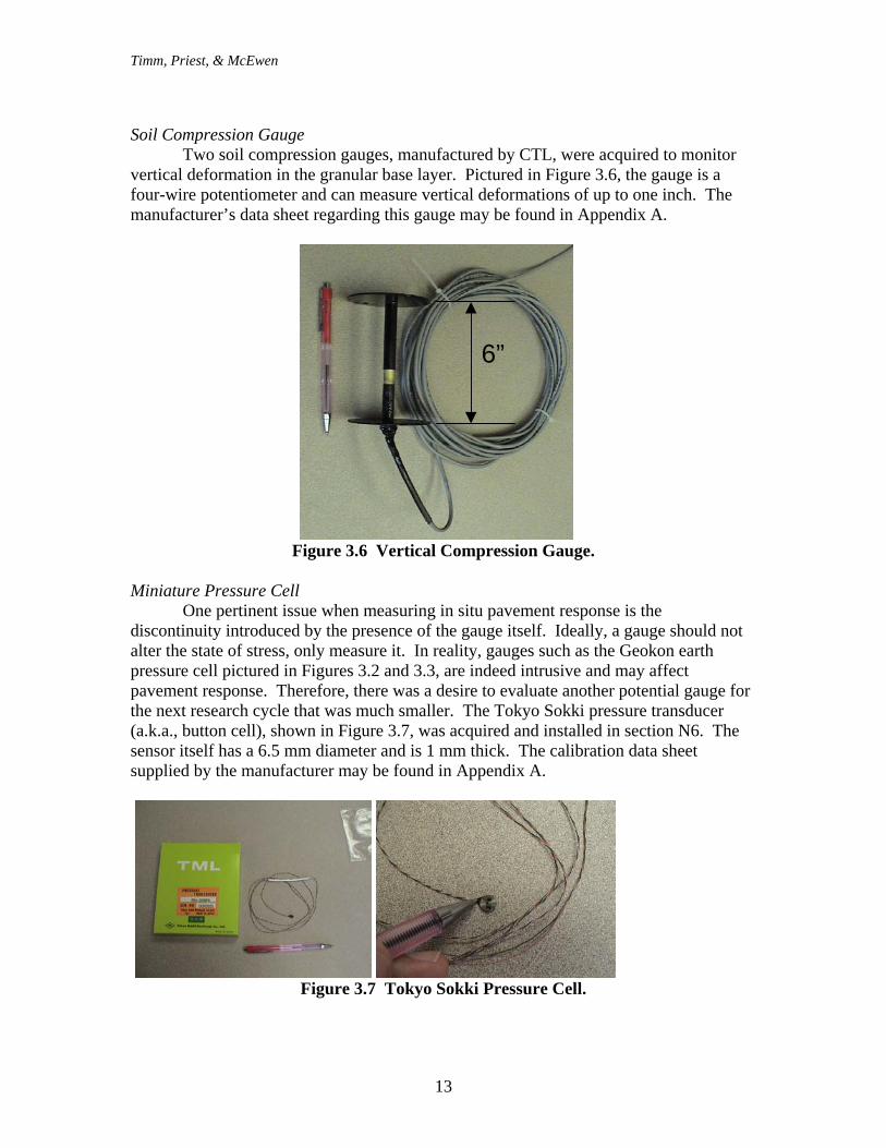
HMA Structural Coefficient (a1) 0.44 Dense Graded Aggregate Base Coefficient (a2) 0.14 Dense Graded Aggregate Base Stiffness 30,000 psi Improved Subgrade Soil Structural Coefficient (a3) 0.05 Improved Subgrade Soil Stiffness 8,000 psi Subgrade Soil Stiffness 5,500 psi

Since the structural sections were meant to be integrated with the existing test sections, shown in Figure 2.1, the total thickness of the new designs had to equal 30 inches (42 inches including the existing improved subgrade). Also, it was decided to use a 6 inch granular base, so the remaining 24 inches were comprised of HMA on the top and improved soil on the bottom. The structural design determined these two values for each of the three traffic levels.

Figure 2.1 Existing Test Track Cross Section (after Jess, 2004).

4” Experimental Mix (varies by section)

6” Asphalt Treated Base (PG76-22)

9” Asphalt Treated Base (PG67-22)

5” Permeable Black Base

6” Dense Crushed Agg. Base

12” Improved Roadbed (A-2)

CL

Layers removed for reconstruction


7

The number of design ESALs were calculated according to the AASHTO methodology for the axle weights given above (Table 2.1) with the 12 kip steer axle treated as a single axle. It is expected that approximately 965,000 laps of the design vehicle will be applied to the sections, and ESALs were computed accordingly. It should be noted that an iterative procedure was used to ensure convergence between the structural number (SN) to determine equivalency factors and the required SN obtained from the AASHTO design equation. As stated above, the objective of the pavement design was to determine the HMA thickness and amount of additional fill. To that end, the following equations were derived and used to find the appropriate thicknesses of each layer. SN = a1D1 + a2D2 + a3(D3 + D4) (2.1) where: a1, a2, a3 are given above D2 = 6 in. D4 = 12 in. (existing) D1 = unknown HMA thickness, in. D3 = unknown additional fill thickness, in. D = D1 + D2 + D3 + D4 (2.2) where: D = 42 in. Once the appropriate SN values were determined for each traffic level, the two above equations were solved for the two unknowns, D1 and D3. Table 2.2 lists the resulting design thicknesses for each of the three traffic levels. Additionally, since all the traffic will be applied to each of the sections, it is instructive to determine the reliability level at one traffic level. For the purposes of this study, reliability at the previous level of ESALs (10 million) are listed in Table 2.2. While these thicknesses were derived directly from the AASHTO Guide, it was thought to be beneficial to expand the range of thicknesses, for experimentation sake, to include more diversity in the cross sections. Therefore, it was recommended to change the thicknesses as shown in Table 2.3 which should aid in distinguishing the sections in terms of structural performance.

Table 2.2 2003 Test Track Structural Sections – Preliminary Design.

Traffic

ESALs, 106 HMA, in.

(D1) GB, in.

(D2) Additional Fill, in.

(D3)

SNReliability at 10*106 ESAL

Full 9.6 9.6 6 14.4 6.4 94.8% 2 / 3 6.3 8.7 6 15.3 6.0 87.9% 1 / 3 3.1 7.2 6 16.8 5.4 67.7%


8

Table 2.3 2003 Test Track Structural Sections – Recommended Design.

Traffic HMA, in.

(D1) GB, in.

(D2) Additional Fill, in.

(D3)

SNReliability at 10*106 ESAL

Full 9 6 15 6.2 92% 2 / 3 7 6 17 5.4 68% 1 / 3 5 6 19 4.6 30%

TEST SECTION LAYOUT As stated previously, the test sections were laid out to minimize construction and rehabilitation efforts. Figure 2.2 summarizes the experimental sections, in addition to the final section assignments (i.e., N1 – N8).

5 5

9 97 7

1 1

6 6

6

6 6 6

2

6

6

64

0

2

4

6

8

10

12

14

16

N1 N2 N3 N4 N5 N6 N7 N8

Thic

knes

s, in

.

Modified HMAUnmodified HMAModified, SMAUnmod Opt + .5%Aggregate Base

Figure 2.2 Final Design and Section Layout.


9

CHAPTER 3 - INSTRUMENTATION: PRE-INSTALLATION

INTRODUCTION This chapter focuses on the instrumentation that was selected and installed as part of the structural experiment. Since this experiment is meant to address mechanistic pavement issues, as explained in Chapter 1, it was critical to have the ability to measure in situ pavement responses under load. Generally speaking, the instrumentation was devised to provide four major responses:

1. Asphalt horizontal strain. 2. Base and subgrade vertical stress. 3. Subgrade moisture. 4. Vertical temperature profiles.

The following sections detail the gauges that were selected, pre-installation activities, a discussion of the data acquisition systems and the instrumentation layout in the pavement sections. SENSOR SELECTION For a mechanistic pavement design experiment, it is well known that there are two primary critical locations to monitor pavement responses under load. These are at the bottom of the asphalt concrete layer and at the top of the unbound granular layers, respectively. Responses in these two locations have been correlated to fatigue cracking and structural rutting, respectively (e.g., Timm and Newcomb, 2003). Therefore, when selecting instrumentation, it was desired to have gauges that would measure responses in these locations. Prior to evaluating instrumentation vendors, experiences from two previous, yet ongoing, instrumented pavement studies were reviewed. The Minnesota Road Research Project (Baker et al., 1994) and the Virginia SmartRoad (Smart Road, 2003) both had extensive literature and web-site information regarding their experiences in instrumenting their respective pavement sections. These served as a starting point for developing the instrumentation plan. When evaluating potential vendors of pavement instrumentation equipment, a number of criteria were used in selecting the final types of gauges. These included: 1. Ability to measure desired responses. 2. Cost. 3. Availability (i.e., delivery times). 4. Reputation for having good reliability. 5. Continuity with previous research efforts at the test track. Asphalt Strain Gauges The purpose of the asphalt strain gauge in the structural experiment is to measure the dynamic strain response at the bottom of the asphalt concrete layer under moving traffic loads. As described above, experiences from the Mn/ROAD and SmartRoad


10

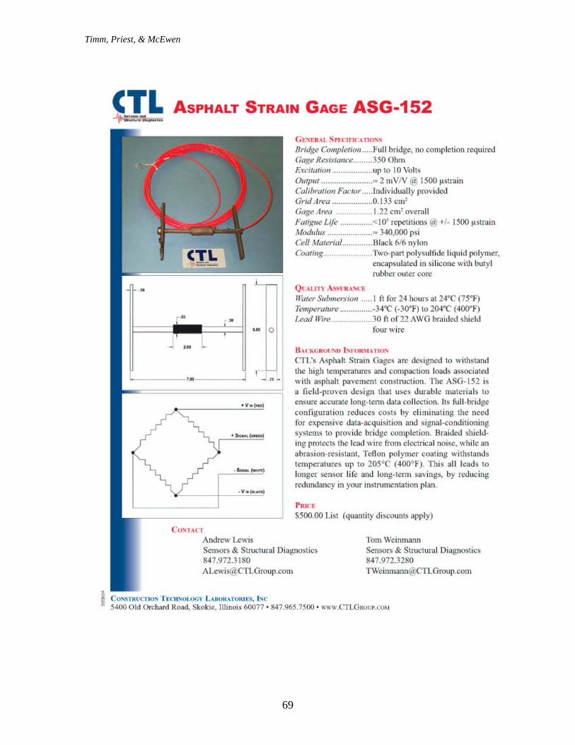
experiments served as a starting point for selection of the asphalt strain gauges. Additionally, experience from the Waterways Experiment Station (i.e., Mr. Thomas McEwen, Mr. Tommy Carr and Dr. Reed Freeman) served as a basis for gauge selection. Vendors such as Dynatest and Tokyo Sokki were evaluated, however their delivery times were prohibitively long to allow them to fit the construction schedule at the test track. Gauges manufactured by Construction Technologies Laboratories (CTL) appeared reasonably priced with a short delivery time and had been widely used to instrument flexible pavements. Therefore, CTL was selected to supply the asphalt strain gauges (ASG). A strain gauge, with dimensions in inches, is shown in Figure 3.1. The data sheet supplied by CTL can be found in Appendix A. The sensor itself is a 350Ω Wheatstone Bridge mounted on a nylon 6/6 bar. There are four active gauges; two aligned with the maximum longitudinal strain and the other two with the transverse strain. The approximate stiffness of the nylon is 340,000 psi. Individual calibration sheets were provided with each gauge. It is also of note that the CTL gauges were designed and constructed to be applicable to most pavement cross-sections. The maximum range on the gauges is ±1,500 µε which is well within expected strain ranges for most flexible pavements.

Figure 3.1 CTL Asphalt Strain Gauge.

Earth Pressure Cells The role of the earth pressure cell is to measure the dynamic vertical pressures generated under moving loads. As will be explained later in this chapter, these gauges were placed at the top of the granular base course and at the top of the subgrade. While it would be advantageous to also measure vertical strain, these type of gauges were not used because of prohibitively high cost. In evaluating pressure cells, vendors such as Kulite and Tokyo Sokki were considered, however Geokon was selected based upon their wide experience in pavement instrumentation. For example, Geokon earth pressure cells were used at Mn/ROAD with good success. The gauge used in this experiment was the Geokon 3500 earth pressure cell. Pictured in Figure 3.2, this device consists of two circular stainless steel plates welded together around their periphery and spaced apart by a narrow cavity filled with de-aired oil. Changing earth pressure squeezes the two plates together causing a corresponding


11

increase of fluid pressure inside the cell. The semi-conductor transducer converts this pressure into an electrical signal which is transmitted as a voltage change via cable to the readout location. Figure 3.3 shows one test cell just after receipt at the test track in addition to the profile of the plate.

Figure 3.2 Geokon Earth Pressure Cell.

Figure 3.3 Geokon Earth Pressure Cell at the Test Track.

For the structural experiment, two different full scale gauges were selected corresponding to the two different expected pressure ranges. Since one set of gauges was installed deeper in the structure (top of subgrade) and the other set was closer to the surface (top of base), 14.5 psi (100 kPa) and 36.3 psi (250 kPa) gauges were selected, respectively. These full scale values were arrived at through a preliminary mechanistic analysis using WESLEA for Windows, a layered elastic pavement analysis computer program (Van Cauwelaert et al., 1989; Timm et al., 1999). Estimates were made regarding material properties and wheel loadings, stresses were calculated at the top of the base and subgrade and it was found that the 14.5 psi and 36.3 psi gauges would work well for the subgrade and base, respectively. Subgrade Moisture Probes In the first research cycle at the Test Track, time domain reflectometry (TDR) probes were used to measure in situ moisture contents throughout the test track. It was decided to continue using these types of probes, supplied by Campbell-Scientific, for the structural experiment. Pictured in Figure 3.4, these gauges were placed in the subgrade of each of the eight structural sections at the Test Track. A full description of these gauges has been previously documented (Freeman, et al., 2001).


12

Figure 3.4 TDR Moisture Probe.

Temperature Profiles Like the moisture probes, the temperature gauges used in the structural experiment were also used during the first research cycle at the Test Track. For each test section, four thermistors were bundled together to provide temperature information near the surface, at 2 in., 4 in. and 10 in. depth. A thermistor bundle is pictured in Figure 3.5, while full descriptions of these gauges may be found is provided by Freeman, et al. (2001).

Figure 3.5 Thermistor Bundle for Measuring In Situ Temperature.

Additional Instrumentation The gauges described above were used in every test section. Additionally, there were two additional kinds of gauges that were included in Cells N2 and N6 to evaluate their effectiveness for use in future research cycles at the test track. Each of these is described below.

2”

4”

10”


13

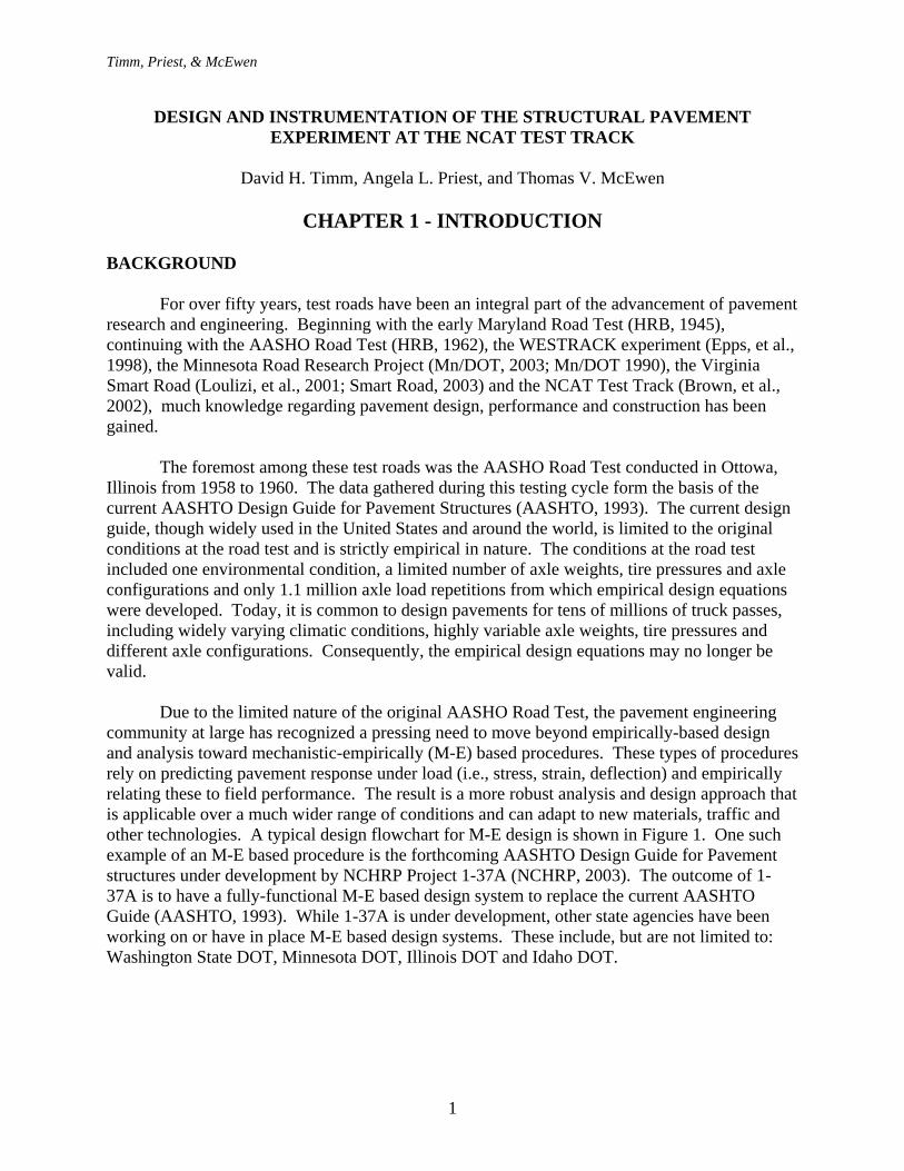
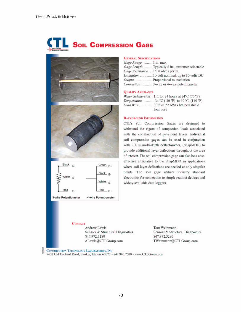
Soil Compression Gauge Two soil compression gauges, manufactured by CTL, were acquired to monitor vertical deformation in the granular base layer. Pictured in Figure 3.6, the gauge is a four-wire potentiometer and can measure vertical deformations of up to one inch. The manufacturer’s data sheet regarding this gauge may be found in Appendix A.

Figure 3.6 Vertical Compression Gauge.

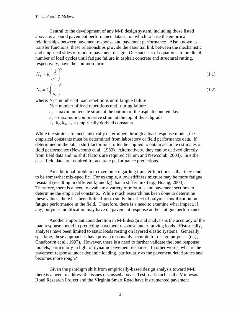
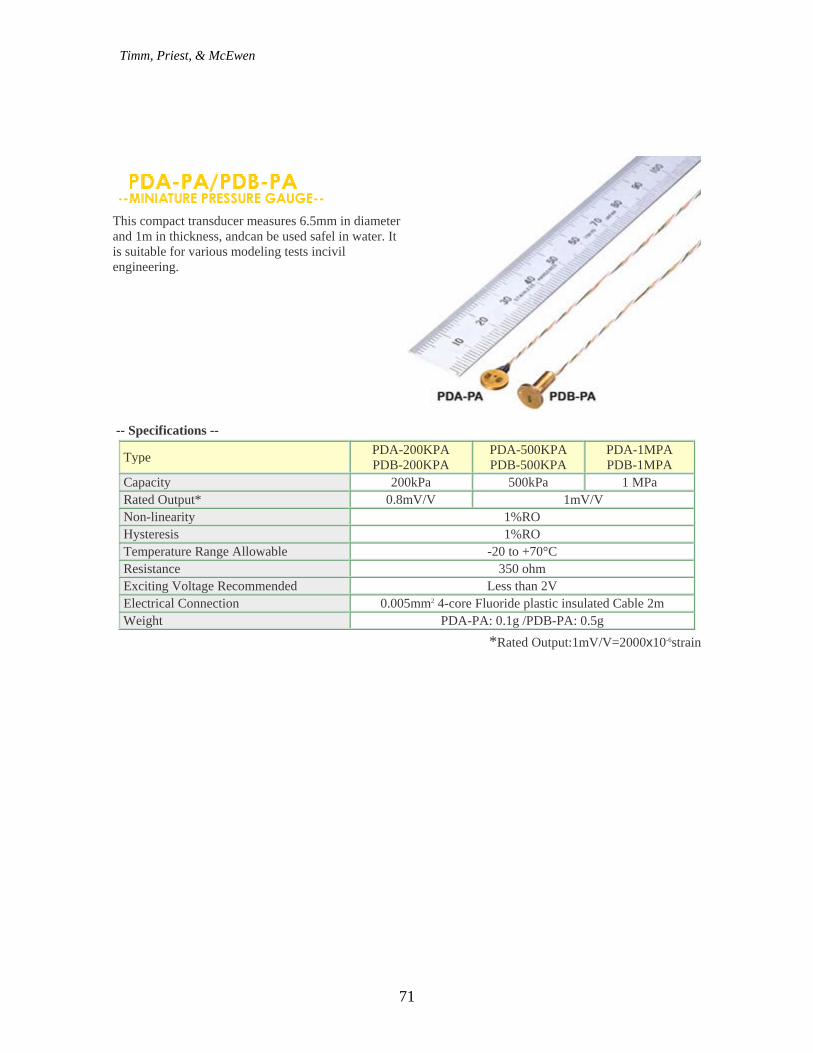
Miniature Pressure Cell One pertinent issue when measuring in situ pavement response is the discontinuity introduced by the presence of the gauge itself. Ideally, a gauge should not alter the state of stress, only measure it. In reality, gauges such as the Geokon earth pressure cell pictured in Figures 3.2 and 3.3, are indeed intrusive and may affect pavement response. Therefore, there was a desire to evaluate another potential gauge for the next research cycle that was much smaller. The Tokyo Sokki pressure transducer (a.k.a., button cell), shown in Figure 3.7, was acquired and installed in section N6. The sensor itself has a 6.5 mm diameter and is 1 mm thick. The calibration data sheet supplied by the manufacturer may be found in Appendix A.

Figure 3.7 Tokyo Sokki Pressure Cell.

6”


14

PREINSTALLATION EFFORTS Prior to installing any of the gauges, each went through a series of checks to ensure that they were working properly. This section details both the functionality and calibration efforts that were conducted prior to installation. Asphalt Strain Gauges There were no facilities at the test track available to fully calibrate the asphalt strain gauges after being received. As was noted above, the calibration of each gauge had already been completed by CTL. However, each gauge was checked for proper functionality at the test track. This was done by connecting each gauge to a Vishay Strain box and pushing and pulling on the gauge to check that the response had the proper sign (i.e., correct polarity). These efforts are illustrated in Figure 3.8. For example, a positive reading corresponded to tension while a negative response corresponded to compression. Also recorded was the “no load” strain box reading. During the functionality checking process, two gauges were identified as non-functioning and were exchanged with the manufacturer for new gauges. In the next research cycle, it would be desirable to have the necessary equipment to perform the calibration on-site and compare against the manufacturer’s values.

Figure 3.8 Strain Gauge Functionality Checks.

Earth Pressure Cells Like the asphalt strain gauges, the earth pressure cells were also checked for functionality. Each was connected and checked that there was a positive voltage change when pushed upon. During these tests, it was found that several of the gauges were either not responding or had reversed polarity. Because of this, in addition to the fact that Geokon did not provide any calibration sheets, it was decided that some kind of calibration needed to be performed. It must be noted that Geokon does provide a general gauge factor for their pressure cells to convert voltage to pressure.


15

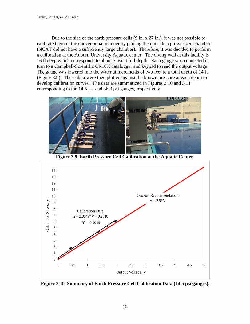
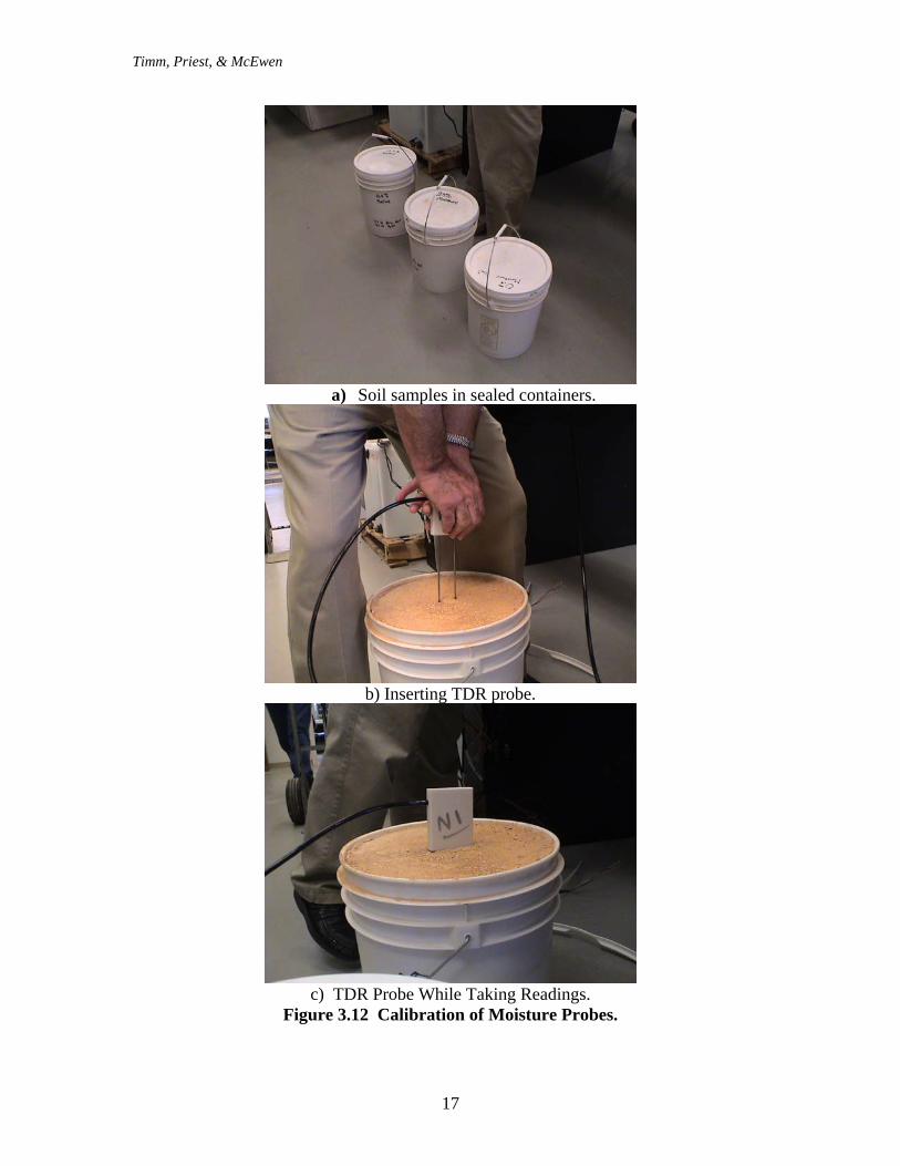
Due to the size of the earth pressure cells (9 in. x 27 in.), it was not possible to calibrate them in the conventional manner by placing them inside a pressurized chamber (NCAT did not have a sufficiently large chamber). Therefore, it was decided to perform a calibration at the Auburn University Aquatic center. The diving well at this facility is 16 ft deep which corresponds to about 7 psi at full depth. Each gauge was connected in turn to a Campbell-Scientific CR10X datalogger and keypad to read the output voltage. The gauge was lowered into the water at increments of two feet to a total depth of 14 ft (Figure 3.9). These data were then plotted against the known pressure at each depth to develop calibration curves. The data are summarized in Figures 3.10 and 3.11 corresponding to the 14.5 psi and 36.3 psi gauges, respectively.

Figure 3.9 Earth Pressure Cell Calibration at the Aquatic Center.

Calibration Dataσ = 3.0049*V + 0.2546

R2 = 0.9946

0123456789

1011121314

0 0.5 1 1.5 2 2.5 3 3.5 4 4.5 5

Output Voltage, V

Cal

cula

ted

Stre

ss, p

si

Geokon Recommendationσ = 2.9*V

Figure 3.10 Summary of Earth Pressure Cell Calibration Data (14.5 psi gauges).


16

Calibration Dataσ = 7.4349*V + 0.2626

R2 = 0.994

0

5

10

15

20

25

30

35

40

0 0.5 1 1.5 2 2.5 3 3.5 4 4.5 5

Output Voltage, V

Pres

sure

, psi Geokon Recommendation

σ = 7.26*V

Figure 3.11 Summary of Earth Pressure Cell Calibration Data (36.3 psi gauges).

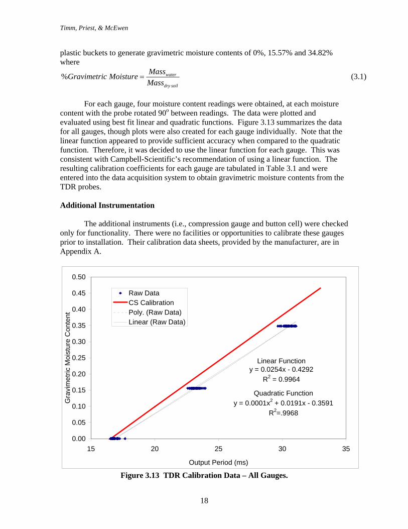
The data shown in Figures 3.10 and 3.11 show that all the gauges responded about the same in the diving well. Best fit lines were run through the data, resulting in the equations and R2 values shown in the figures. Though there did appear to be a slight offset from the manufacturer’s recommendation, the slopes of each plot were very close to the recommended values. One limitation of this experiment was that it only stressed the gauges to ½ and ¼ scale, respectively. Presumably, they would have continued to respond in a linear fashion, and this is what the manufacturer has reported. After reviewing the data, it was decided to proceed with the manufacturer’s recommendation of simply dividing the full scale pressure by the full scale voltage output (5 V) to obtain the gauge calibration factor in units of psi / Volt. In the future, it would be advantageous to have a larger scale pressure chamber on hand to calibrate gauges of this type, and check them throughout their respective ranges. Subgrade Moisture Probes The subgrade moisture probes (TDRs) were calibrated using roadbed soil from the Test Track at three known moisture contents in the laboratory (see Figure 3.12). The soil samples were well mixed with various amounts of moisture and compacted within


17

a) Soil samples in sealed containers.

b) Inserting TDR probe.

c) TDR Probe While Taking Readings.

Figure 3.12 Calibration of Moisture Probes.


18

plastic buckets to generate gravimetric moisture contents of 0%, 15.57% and 34.82% where

soildry

water

MassMassMoisturecGravimetri =% (3.1)

For each gauge, four moisture content readings were obtained, at each moisture content with the probe rotated 90o between readings. The data were plotted and evaluated using best fit linear and quadratic functions. Figure 3.13 summarizes the data for all gauges, though plots were also created for each gauge individually. Note that the linear function appeared to provide sufficient accuracy when compared to the quadratic function. Therefore, it was decided to use the linear function for each gauge. This was consistent with Campbell-Scientific’s recommendation of using a linear function. The resulting calibration coefficients for each gauge are tabulated in Table 3.1 and were entered into the data acquisition system to obtain gravimetric moisture contents from the TDR probes. Additional Instrumentation The additional instruments (i.e., compression gauge and button cell) were checked only for functionality. There were no facilities or opportunities to calibrate these gauges prior to installation. Their calibration data sheets, provided by the manufacturer, are in Appendix A.

Quadratic Functiony = 0.0001x2 + 0.0191x - 0.3591

R2=.9968

Linear Functiony = 0.0254x - 0.4292

R2 = 0.9964

0.00

0.05

0.10

0.15

0.20

0.25

0.30

0.35

0.40

0.45

0.50

15 20 25 30 35

Output Period (ms)

Gra

vim

etric

Moi

stur

e C

onte

nt

Raw DataCS CalibrationPoly. (Raw Data)Linear (Raw Data)

Figure 3.13 TDR Calibration Data – All Gauges.


19

Table 3.1 TDR Probe Calibration Coefficients.

Sensor

Slope Moisture Content / Period (ms)

Intercept Moisture Content

R2

N1 0.0253 -0.4286 0.9980 N2 0.0246 -0.4174 0.9972 N3 0.0261 -0.4401 0.9985 N4 0.0264 -0.4481 0.9975

N5A 0.0252 -0.4255 0.9969 N5B 0.0261 -0.4456 0.9937 N5C 0.0249 -0.4187 0.9987 N6 0.0244 -0.4079 0.9986 N7 0.0260 -0.4419 0.9962 N8 0.0253 -0.4277 0.9991

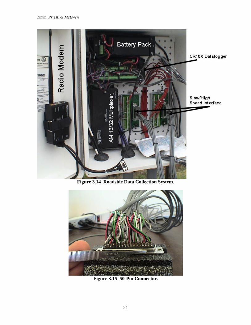
DATA ACQUISITION One feature of the instrumentation described above is that they combine both high and slow speed measurement requirements. For example, the moisture and temperature probes can be sampled at a relatively slow frequency, say once per minute, without missing any important information. However, the sampling rate required for the strain gauges, pressure cells, button cell and compression gauges is much higher due to the dynamic nature of the traffic loading. The duration of loading under live traffic may be in the range of 20 to 100 millisecond, depending upon vehicle speed. Therefore, there is a need to have a much higher sampling rate, on the order of thousands of samples per second. Another feature of the instrumentation described above is that it will not be necessary to measure the dynamic pavement response under every truck pass. Since the traffic stream at the Track is very well controlled (5 tractor-trailer combinations with known weights), it will only be necessary to measure dynamic pavement responses periodically. It is currently estimated that this will be at least once per month and more frequently once pavement distresses are observed. With the two features in mind, a data acquisition plan was devised to record both slow speed and high speed data throughout the structural experiment. Except when conducting high speed data collection, all of the sensors will be connected to the slow speed collection system. For high speed data collection, the strain gauges, earth pressure cells, compression gauges and button cell will be disconnected from the slow speed system and wired into the high speed data acquisition system. A discussion of the slow and high speed systems is below. Slow Speed Data Acquisition Since the structural experiment had to be integrated with the existing infrastructure at the track, it was decided to continue using Campbell-Scientific


20

dataloggers to record slow speed data. The CR10X datalogger, AM 16/32 Multiplexer and battery pack were mounted in each of the roadside boxes. A solar panel was mounted above each box to recharge the battery pack during daylight hours. Additionally, an RF400 radio modem was mounted to transmit the slow speed data wirelessly from the roadside to the research building at the Track. The radio modem represented a significant change from the first research cycle where conduit was laid and all boxes were connected to the research building by hardwire. The advantages of using a radio modem, enumerated below, were impetus for using them in the structural experiment: 1. Long conduit lines not needed saving significant trenching work. 2. Each box is isolated so that if one is hit by lightning, the others remain unaffected. 3. No conduit lines to be damaged in the event of a vehicle going off the track. It is expected that the Track will be entirely wireless in the next research cycle (2006). The slow speed equipment is pictured in Figure 3.14. The two silver 50-pin connectors shown in Figure 3.14 serve as the interface between the slow and high speed systems. It should be noted that 50-pin connectors were assembled entirely by the instrumentation consultant and Track research personnel. A partially completed connector, with housing removed is pictured in Figure 3.15. When collecting high speed data, these two cables will be disconnected and replaced with two other 50-pin connectors running to the high speed data acquisition system described below. Data collected using the slow speed system will be sampled at 1 sample per minute using Campbell-Scientific Loggernet software. Hourly average, minimum and maximum tables will then be generated to track the slower, yet transient phenomena.


21

Figure 3.14 Roadside Data Collection System.

Figure 3.15 50-Pin Connector.


22

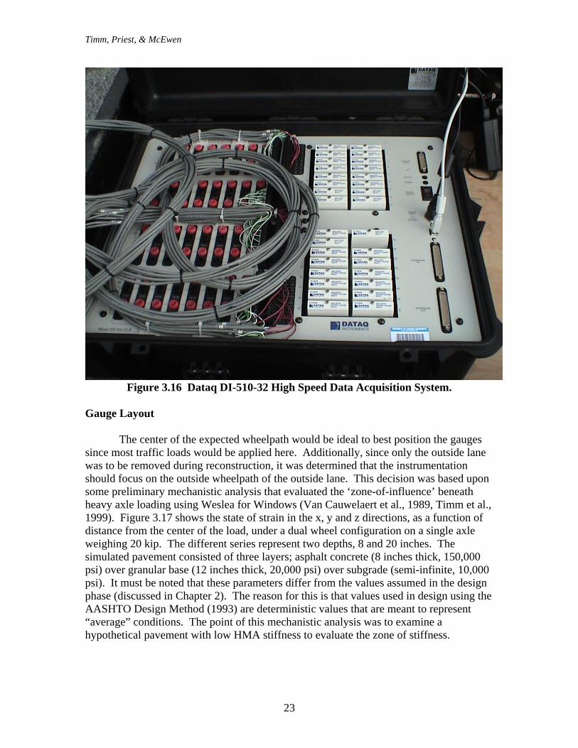
High Speed Data Acquisition When developing the instrumentation plan, it was estimated that sampling rates as high as 10,000 samples/sec/channel may be required during dynamic testing. To that end, a number of systems were evaluated for their use at the Track. When deciding upon a system, the following criteria were considered: 1. Is the system capable of handling up to 10,000 samples/sec/channel? 2. Is the system portable so that it may be connected and disconnected with ease to each

section? 3. Is the system easy to program and use? 4. What is the cost of the system? After evaluating a variety of systems, it was decided to acquire a Dataq DI-510-32 high-speed data acquisition system. This system is pictured in Figure 3.16. One of the most important features of this system is that the acquisition software is entirely menu driven with point-and-click ‘programming’. This enables the researchers to have the system up and running quickly and make modifications to programs as necessary without consulting an expert programmer. Additional features of the Dataq system include: 1. Sampling rates up to 250,000 Hz. 2. Real-time, on screen, data visualization. 3. Capable of handling all the sensors previously described. 4. Affordability such that an additional backup system may be purchased in the future

within the current operating budget. 5. Portability such that the system can be run off the power inverter mounted on the

Track golf cart. As shown in Figure 3.16, indicated by the white rectangular cards, there are 32 available channels on the Dataq system. These cards serve as modules to control each of the sensors connected to the system. Each provides the required excitation voltage and amplification as required by each sensor. The entire system was configured such that it could simply be plugged into each section’s box, using the 50-pin connectors shown in Figure 3.14 and begin collecting data. HIGH SPEED SENSOR LAYOUT AND LABELING When developing the instrumentation plan, two factors played a primary roll. First, as one would expect, it was necessary to place the instruments where they would be trafficked by the vehicles. Second, there needed to be a certain level of redundancy in each test cell in case gauges became dysfunctional during installation, construction or full operation of the facility. This section details the location and labeling of all the instrumentation with attention to the above two issues.


23

Figure 3.16 Dataq DI-510-32 High Speed Data Acquisition System.

Gauge Layout The center of the expected wheelpath would be ideal to best position the gauges since most traffic loads would be applied here. Additionally, since only the outside lane was to be removed during reconstruction, it was determined that the instrumentation should focus on the outside wheelpath of the outside lane. This decision was based upon some preliminary mechanistic analysis that evaluated the ‘zone-of-influence’ beneath heavy axle loading using Weslea for Windows (Van Cauwelaert et al., 1989, Timm et al., 1999). Figure 3.17 shows the state of strain in the x, y and z directions, as a function of distance from the center of the load, under a dual wheel configuration on a single axle weighing 20 kip. The different series represent two depths, 8 and 20 inches. The simulated pavement consisted of three layers; asphalt concrete (8 inches thick, 150,000 psi) over granular base (12 inches thick, 20,000 psi) over subgrade (semi-infinite, 10,000 psi). It must be noted that these parameters differ from the values assumed in the design phase (discussed in Chapter 2). The reason for this is that values used in design using the AASHTO Design Method (1993) are deterministic values that are meant to represent “average” conditions. The point of this mechanistic analysis was to examine a hypothetical pavement with low HMA stiffness to evaluate the zone of stiffness.


24

-250

-200

-150

-100

-50

0

50

100

150

200

250

0 10 20 30 40 50 60 70 80 90

Distance from Center of Interior Tire, in.

Nor

mal

Mic

rost

rain

X - Depth = 8 X - Depth = 20

Y - Depth = 8 Y - Depth = 20

Z - Depth = 8 Z - Depth = 20

Figure 3.17 Zone of Influence Evaluation.

Note that all strains attenuate as distance from the load increases. However even at a distance of 80 inches, there still is a strain response. Certainly, closer to the load, there are much more dramatic changes in strain with distance from the center of the load. This graph, and others like it, were reviewed and used to determine that the discontinuity posed by the existing inside lane left in place could dramatically affect the pavement response under load. Therefore, as mentioned above, gauges were placed in the outside wheelpath of the outside lane. This also served as additional impetus for removing the entirety of the outside lane and shoulder, rather than just the area between the centerline and edge stripe. Complete removal of the existing shoulder also aided in restoring adequate drainage conditions on the structural sections. Had the shoulder been left in place, water entering the pavement surface would have met the relatively impermeable HMA in the shoulder creating a “bath tub” condition. Locating the center of the wheelpath posed a special challenge in of itself. Since the structural sections began at the end of the east curve and continued down the north tangent, the wheel path tended to vary as the trailers aligned themselves coming out of the curve. Therefore, it was not simply a matter of determining one offset distance from the centerline to the wheelpath. Rut depth measurements obtained from the previous research cycle at the test track were reviewed and used to determine the transverse location of maximum rutting, which is the most probable location of the wheelpath and where the instrumentation was to be placed in each test cell. After full-depth removal of the existing pavement, each test cell was marked to indicate the transverse offset from the


25

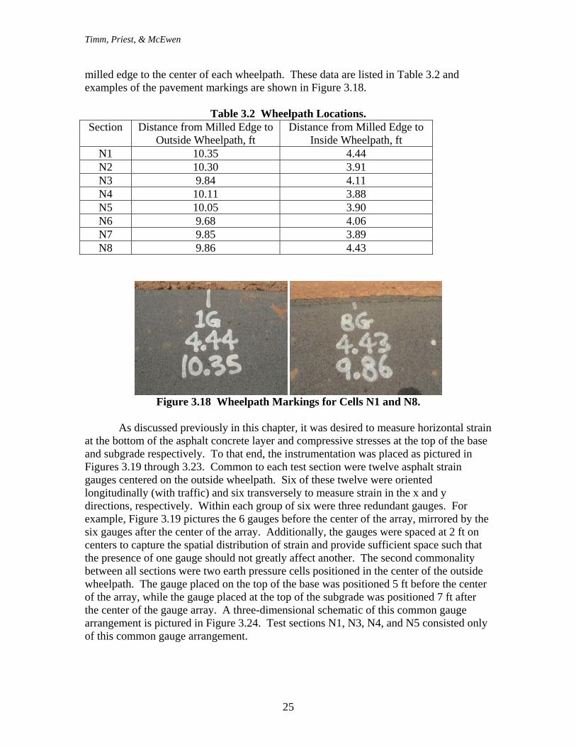
milled edge to the center of each wheelpath. These data are listed in Table 3.2 and examples of the pavement markings are shown in Figure 3.18.

Table 3.2 Wheelpath Locations. Section Distance from Milled Edge to

Outside Wheelpath, ft Distance from Milled Edge to

Inside Wheelpath, ft N1 10.35 4.44 N2 10.30 3.91 N3 9.84 4.11 N4 10.11 3.88 N5 10.05 3.90 N6 9.68 4.06 N7 9.85 3.89 N8 9.86 4.43

Figure 3.18 Wheelpath Markings for Cells N1 and N8.

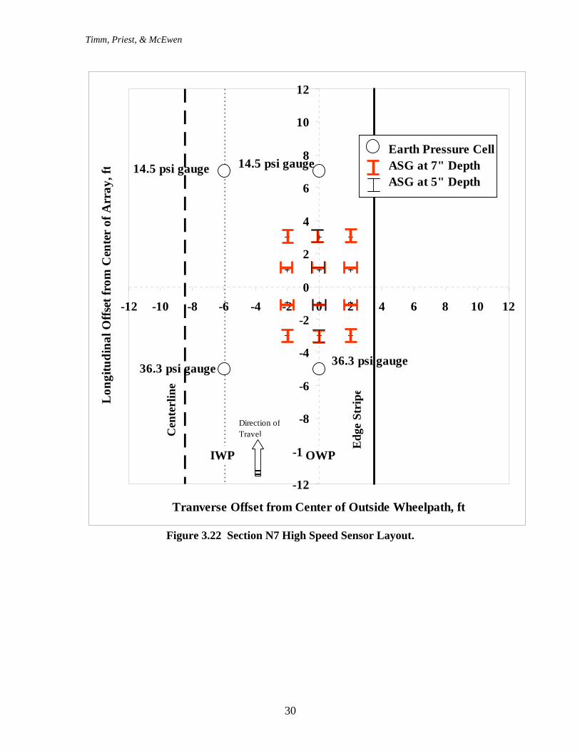
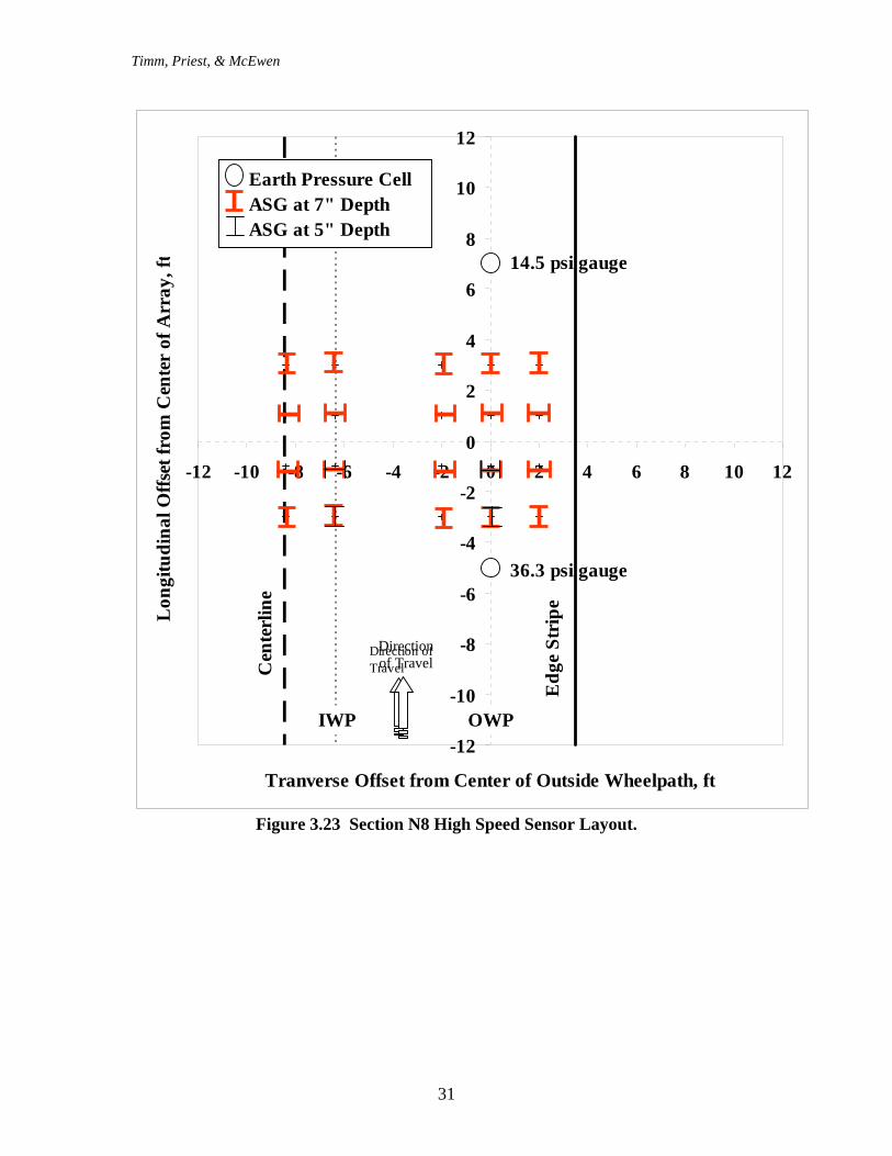
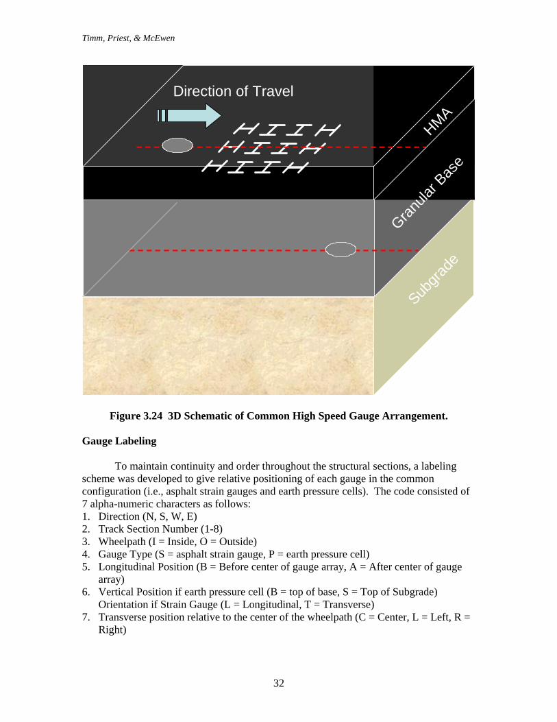
As discussed previously in this chapter, it was desired to measure horizontal strain at the bottom of the asphalt concrete layer and compressive stresses at the top of the base and subgrade respectively. To that end, the instrumentation was placed as pictured in Figures 3.19 through 3.23. Common to each test section were twelve asphalt strain gauges centered on the outside wheelpath. Six of these twelve were oriented longitudinally (with traffic) and six transversely to measure strain in the x and y directions, respectively. Within each group of six were three redundant gauges. For example, Figure 3.19 pictures the 6 gauges before the center of the array, mirrored by the six gauges after the center of the array. Additionally, the gauges were spaced at 2 ft on centers to capture the spatial distribution of strain and provide sufficient space such that the presence of one gauge should not greatly affect another. The second commonality between all sections were two earth pressure cells positioned in the center of the outside wheelpath. The gauge placed on the top of the base was positioned 5 ft before the center of the array, while the gauge placed at the top of the subgrade was positioned 7 ft after the center of the gauge array. A three-dimensional schematic of this common gauge arrangement is pictured in Figure 3.24. Test sections N1, N3, N4, and N5 consisted only of this common gauge arrangement.


26

As discussed previously, the compression gauges were meant to be evaluated for potential use in the next round of structural experimentation at the Test Track. Therefore, having only two gauges, it was decided to place them in the test section where they would likely undergo the most amount of deformation. Since section N2 was the thinnest section with unmodified binder, the gauges were placed in the center of the inside and outside wheelpaths as shown in Figure 3.20. Comparisons will be made between the gauges to ascertain the effect of the milled edge, from a mechanistic standpoint, near the inside wheelpath. Like the compression gauges, the button cell was another gauge under evaluation. While one could argue about which cell to place it in, it was decided that the important factor was to place it in close proximity to an earth pressure cell. The purpose of this was to evaluate differences between the two types of gauges measuring the same stresses in the same material. Figure 3.21 shows the button cell was placed in section N6 with the 36.3 psi earth pressure cell. A more detailed discussion of the placement of this gauge will be presented in the next chapter on sensor installation. As already discussed, there is a need to evaluate the effect of the milled edge, near the inside wheelpath, on pavement response. Therefore, pressure cells were placed in the inside and outside wheelpaths of section N7, as shown in Figure 3.22, so that comparisons may be made. Section N8 also had duplicate strain gauges in the inside wheelpath, as shown in Figure 3.23. It should be noted that it was not possible to place gauges to the right of the inside wheelpath due to the configuration of the paver wheels. A more complete discussion of this issue is presented in the next chapter on sensor installation. Recall from Chapter 2 that section N8 was designed with the so-called ‘rich-bottom’ so there was a need to evaluate what effect this might have on the pavement response under load. Therefore, in addition to gauges in the common configuration, gauges were also placed on top of the rich bottom, in each wheelpath to maintain symmetry as shown in Figure 3.23. Gauges were also placed on top of the bottom unmodified lift in section N7 to serve as a basis of comparison to section N8. These gauges are depicted in Figure 3.22.


27

-12

-10

-8

-6

-4

-2

0

2

4

6

8

10

12

-12 -10 -8 -6 -4 -2 0 2 4 6 8 10 12

Tranverse Offset from Center of Outside Wheelpath, ft

Lon

gitu

dina

l Offs

et fr

om C

ente

r of

Arr

ay, f

t

Earth Pressure CellAsphalt Strain Gage

36.3 psi gauge

14.5 psi gauge

OWPIWP

Cen

terl

ine

Edg

e St

ripe

Direction of Travel

Figure 3.19 Sections N1, N3, N4, N5 High Speed Sensor Layout.


28

-12

-10

-8

-6

-4

-2

0

2

4

6

8

10

12

-12 -10 -8 -6 -4 -2 0 2 4 6 8 10 12


Lon

gitu

dina

l Offs

et fr

om C

ente

r of

Arr

ay, f

t

Earth Pressure CellAsphalt Strain GageCompression Gage

36.3 psi gauge

14.5 psi gauge

OWPIWP

Cen

terl

ine

Edg

e St

ripe

Direction of Travel

Figure 3.20 Section N2 High Speed Sensor Layout.


29

-12

-10

-8

-6

-4

-2

0

2

4

6

8

10

12

-12 -10 -8 -6 -4 -2 0 2 4 6 8 10 12


Lon

gitu

dina

l Offs

et fr

om C

ente

r of

Arr

ay, f

t

Earth Pressure CellAsphalt Strain GageButton Cell

36.3 psi gauge

14.5 psi gauge

OWPIWP

Cen

terl

ine

Edg

e St

ripe

Direction of Travel



30

-12

-10

-8

-6

-4

-2

0

2

4

6

8

10

12

-12 -10 -8 -6 -4 -2 0 2 4 6 8 10 12


Lon

gitu

dina

l Offs

et fr

om C

ente

r of

Arr

ay, f

t

36.3 psi gauge

14.5 psi gaugeEarth Pressure CellASG at 7" DepthASG at 5" Depth

14.5 psi gauge

36.3 psi gauge

OWPIWP

Cen

terl

ine

Edg

e St

ripe

Direction of Travel



31

-12

-10

-8

-6

-4

-2

0

2

4

6

8

10

12

-12 -10 -8 -6 -4 -2 0 2 4 6 8 10 12


Lon

gitu

dina

l Offs

et fr

om C

ente

r of

Arr

ay, f

tEarth Pressure CellASG at 7" DepthASG at 5" Depth

36.3 psi gauge

14.5 psi gauge

OWPIWP

Cen

terl

ine

Edg

e St

ripe

Direction of Travel


Direction of Travel


32

Figure 3.24 3D Schematic of Common High Speed Gauge Arrangement.

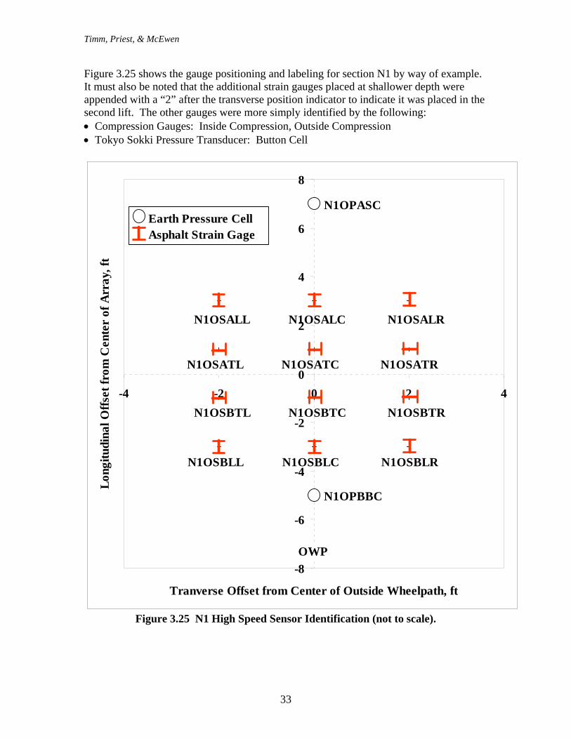
Gauge Labeling To maintain continuity and order throughout the structural sections, a labeling scheme was developed to give relative positioning of each gauge in the common configuration (i.e., asphalt strain gauges and earth pressure cells). The code consisted of 7 alpha-numeric characters as follows: 1. Direction (N, S, W, E) 2. Track Section Number (1-8) 3. Wheelpath (I = Inside, O = Outside) 4. Gauge Type (S = asphalt strain gauge, P = earth pressure cell) 5. Longitudinal Position (B = Before center of gauge array, A = After center of gauge

array) 6. Vertical Position if earth pressure cell (B = top of base, S = Top of Subgrade)

Orientation if Strain Gauge (L = Longitudinal, T = Transverse) 7. Transverse position relative to the center of the wheelpath (C = Center, L = Left, R =

Right)

HMA

Granula

r Bas

e

Subgra

de

Direction of Travel

HMA

Granula

r Bas

e

Subgra

de

Direction of Travel

HMA

Granula

r Bas

e

Subgra

de

Direction of Travel


33

Figure 3.25 shows the gauge positioning and labeling for section N1 by way of example. It must also be noted that the additional strain gauges placed at shallower depth were appended with a “2” after the transverse position indicator to indicate it was placed in the second lift. The other gauges were more simply identified by the following: • Compression Gauges: Inside Compression, Outside Compression • Tokyo Sokki Pressure Transducer: Button Cell

-8

-6

-4

-2

0

2

4

6

8

-4 -2 0 2 4


Long

itudi

nal O

ffset

from

Cen

ter

of A

rray

, ft

Earth Pressure CellAsphalt Strain Gage

OWP

N1OSBLL N1OSBLC N1OSBLR

N1OSBTL N1OSBTC N1OSBTR

N1OSALL N1OSALC N1OSALR

N1OSATL N1OSATC N1OSATR

N1OPBBC

N1OPASC

Figure 3.25 N1 High Speed Sensor Identification (not to scale).


34

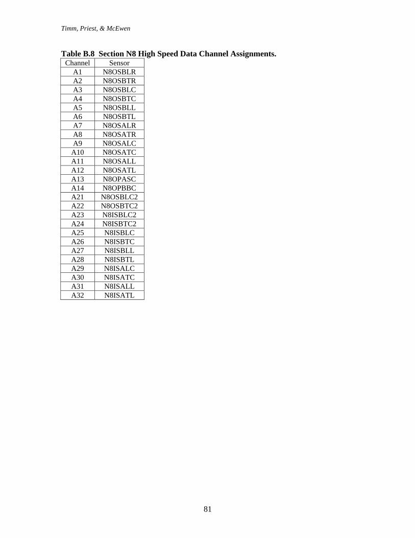
Each gauge was labeled according to its location prior to installation. Labels were placed on the wire near the gauge itself in addition to the end of the cable to enable easy gauge identification during placement and installation. Figure 3.26 depicts this process. Recall that each of these ‘high-speed’ gauges were also to be connected to Dataq acquisition system. The channel assignments for the Dataq system are contained in tables in Appendix B.

Figure 3.26 Gauge Labeling using Heat Gun and Shrink Tubing.

TEMPERATURE AND MOISTURE GAUGE POSITIONING One temperature probe, as pictured in Figure 3.5 was placed in each section. These were centered between the outside lane edge stripe and rumble strips approximately 3 feet after the center of the gauge array. A full discussion of their installation is provided in the next chapter. Test sections N1 through N4 and N6 through N7 had one moisture probe each. These were placed approximately 3 inches below the top of the subgrade centered between the wheelpaths. In section N5, which contained three moisture probes at three depths, the final placement of the gauges was at 3", 15", and 27" into subgrade, respectively.


35

SUMMARY This chapter focused upon the instrumentation itself; namely the functioning of each gauge in addition to its relative location within each test section. The next chapter deals with construction and installation issues pertaining to these gauges.


36

CHAPTER 4 - SENSOR INSTALLATION

INTRODUCTION This chapter details construction of the eight sections comprising the structural experiment at the NCAT Test Track, with focus placed upon sensor installation. For more information regarding the actual construction of the sections, please refer to (Powell, 2004). It must be noted that prior to installation, reports from the Minnesota Road Research Project (Baker, et al., 1994) and the Virginia Smart Road (Smart Road, 2003), in addition to the manufacturer’s recommendations, were consulted in determining the best installation procedures. Another note of interest is that the sensor installation was completely integrated with the contractor’s construction schedule. At no time during the process was construction held up due to installation of sensors. The following sections follow more or less chronologically, detailing the installation of the pavement sensors. SUBGRADE MOISTURE PROBES AND EARTH PRESSURE CELLS Once the contractor had brought the improved roadbed to the correct elevation and density, TDR moisture probes and 14.5 psi earth pressure cells were installed in each test section. Refer to Chapter 3 for the precise location of each gauge. TDR Moisture Probes Using string lines, the moisture probe locations were marked in each test section. Cavities were dug by hand approximately 8 in. wide by 24 in. long by 6 in. deep to accommodate the TDR probes. In section N5, which contained three moisture probes at three depths, cavities were dug so that final placement of the gauges would be at 3", 15", and 27" into subgrade, respectively. Cable trenches were then excavated by hand 3 in. wide by 2 in. deep running from the cavity to the edge of the pavement. The cavities and trenches were brushed clean to eliminate any sharp stone fragments that could damage the cables or instruments. An example of the cavity, cable trench and cleaning is pictured in Figure 4.1. After the trenches and cavities had been cleaned, the cavities were partially filled with minus #4 subgrade material. Each was filled with three 1-inch lifts, compacted with a standard Marshall hammer to ensure density. The trenches were partially filled with a crushed granite material (used in the base course) passing a #8 sieve. A portion of the filling procedure is shown in Figure 4.2.


37

Figure 4.1 TDR and Earth Pressure Cell Cavities and Trenches.

Marshall Hammer

-#4 SubgradeFill Material - #8 Trench Fill

Marshall Hammer

-#4 SubgradeFill Material - #8 Trench Fill

Figure 4.2. Compacting TDR Cavity and Backfilled Cable Trenches.

Following the cavity backfilling process, the TDR gauges were placed such that the metal probes ran parallel to the direction of traffic. The gauges were oriented so that approaching traffic would tend to push the cable connection into the probe to help secure the connection during construction and ensuing trafficking. It was also important to maintain some slack in the cable in the hole to provide strain relief. The cables were then


38

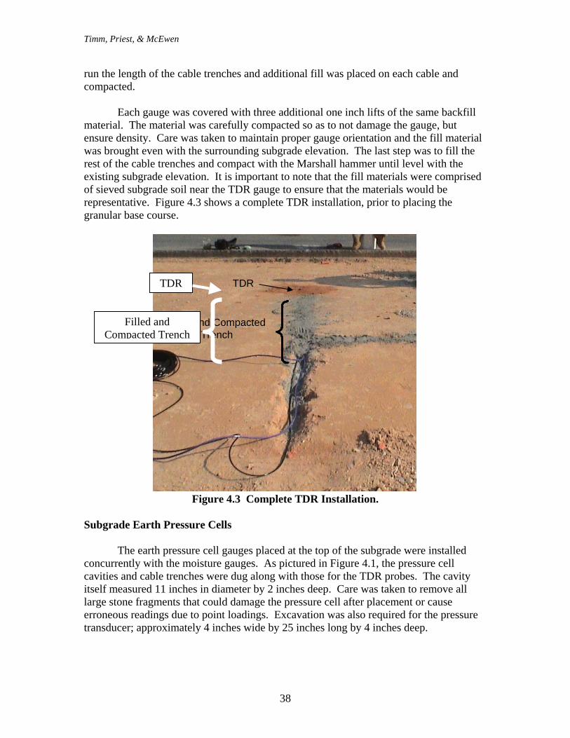
run the length of the cable trenches and additional fill was placed on each cable and compacted. Each gauge was covered with three additional one inch lifts of the same backfill material. The material was carefully compacted so as to not damage the gauge, but ensure density. Care was taken to maintain proper gauge orientation and the fill material was brought even with the surrounding subgrade elevation. The last step was to fill the rest of the cable trenches and compact with the Marshall hammer until level with the existing subgrade elevation. It is important to note that the fill materials were comprised of sieved subgrade soil near the TDR gauge to ensure that the materials would be representative. Figure 4.3 shows a complete TDR installation, prior to placing the granular base course.

TDR

Filled and CompactedTrench

TDR

Filled and CompactedTrench

Figure 4.3 Complete TDR Installation.

Subgrade Earth Pressure Cells The earth pressure cell gauges placed at the top of the subgrade were installed concurrently with the moisture gauges. As pictured in Figure 4.1, the pressure cell cavities and cable trenches were dug along with those for the TDR probes. The cavity itself measured 11 inches in diameter by 2 inches deep. Care was taken to remove all large stone fragments that could damage the pressure cell after placement or cause erroneous readings due to point loadings. Excavation was also required for the pressure transducer; approximately 4 inches wide by 25 inches long by 4 inches deep.

TDR

Filled and Compacted Trench


39

The cavity preparation required the use of sieved granular base material. The bottom 1 inch of the cavity was filled and compacted with minus #8 base material and brought to level. The next 0.75 inches were filled with a minus #16 loose sand. The finer material was used to ensure that no large particles would come into contact with the pressure plate. To obtain accurate readings, it was critical that the cell was properly leveled and had no air voids under the plate. Prior to placing the pressure cell, the stem from the plate to the transducer was bent at a slight angle. This was to make sure the transducer would have added protection and reside primarily in the excavated area and not protrude into the base course. Once the cell was ready, it was placed on top of the -#16 material and checked for level. Also, the cell was removed to inspect whether there were any voids beneath the gauge by examining the cell imprint in the fine material. This process was repeated until the gauge was level, resided approximately 0.25 inches below the existing elevation, and had no voids beneath it. The cell leveling process is illustrated in Figure 4.4. Also of note in Figure 4.4 is the trench material used in the transducer excavation area (to the left of the pressure plate). It was critical to have this material loosely in place to act as a support to bring the plate to level.

Figure 4.4 Leveling Subgrade Earth Pressure Cell.

After leveling the gauge, additional fill material was placed by hand around the transducer and carefully compacted. Cables were placed in the already backfilled trenches, using the same procedure as that for the TDR probes. Additional material was placed on top of the cables, compacted with the Marshall hammer and brought to grade. Prior to completely covering the pressure cell, an initial no load reading was taken. These will be used later in determining overburden stresses with time. Finally, additional fine sand material (-#16) was carefully placed on top of the exposed pressure


40

plate until the existing grade was met. Figure 4.5 illustrates a completed earth pressure cell installation.

Figure 4.5 Completed Earth Pressure Cell Installation.

The work described above (TDRs and earth pressure cells) took approximately two full days to complete all eight sections. Difficulties were encountered in digging the trenches; the subgrade material contained many stone fragments that tended to wear on tools and the hands that bore them. Additionally, there was a learning process since none of the personnel involved had installed these gauges previously. Success in this part of the installation was ensured through great attention to detail and a willingness to work with each gauge until it was installed properly. Granular Base Layer Construction Once all the gauges had been placed in the subgrade, the contractor was ready to construct the granular base course. However, the gauges required some minimum amount of protection from the trucks, bulldozers and rollers used in the process. To achieve this, a thick layer of granular base material was placed by hand on top of each sensor and cable trench throughout the eight test sections. The material was sieved through a #4 screen to be sure no large particles would damage the gauges. The hand placement of the base material is depicted in Figure 4.6. During the construction of the base course, care was taken by the contractor to make sure the dump trucks did not roll directly over any of the gauges. Temporary ramps made of base material were constructed so that the dump trucks could move from the inside lane to the outside lane without traveling over any of the gauges. The gauges were monitored for survivability during the base construction as pictured in Figure 4.7.

Pressure Cell Protected from Foot/Vehicle Traffic

Obtaining No-load reading

Pressure Cell Protected from Foot/Vehicle Traffic

Obtaining No-load reading


41

Though no gauges were lost or damaged during the base construction, in the future it may be advantageous to use side-dump trucks to take advantage of the inside lane serving as a work platform and guarantee that no dump trucks would damage any gauges.

a) Sieving Granular Base for Cover

b) #4 Screen to Sieve Cover Material

c) Placing Cover Material by Shovel Figure 4.6 Hand Placement of Granular Base Material.


42

Earth Pressure Cell and TDR AreaEarth Pressure Cell and TDR Area

Figure 4.7 Base Construction and Gauge Monitoring.

BASE PRESSURE AND BUTTON CELLS , ASPHALT STRAIN AND COMPRESSION GAUGES Gauge Marking and Excavation Once the contractor had completed construction of the granular base course, installation of the 36.3 psi earth pressure cells, button cell, asphalt strain gauges and compression gauges began. These gauges were installed concurrently to utilize common cable trenches thereby minimizing disruption of the base material. The first step in placing the sensors was to carefully locate the center of the gauge array. The center was defined as the center of the outside wheelpath (refer to Table 3.2) crossed by the center of a line extending from the junction box containing the dataloggers. Stringlines were run from surveyed points to establish the center of the outside wheelpath and the center of the junction box. A plywood template (4 ft x 8 ft) made prior to construction was then oriented on the center of the array and asphalt strain gauge locations were marked. The template allowed for rapid and consistent placement of the gauge locations which was important in minimizing disruption to the contractor and the project as a whole. Setting the locations is depicted in Figure 4.8. The template was then removed and additional markings were added to help orient the strain gauges along the longitudinal and transverse directions. Finally, markings for the earth pressure


43

cells, button cell, and compression gauges were placed. An example of the final markings is shown in Figure 4.9.

a) Setting String Lines

b) Centering Template Figure 4.8 Establishing Center of Gauge Array and ASG Locations.

Figure 4.9 Gauge Location Markings for Cell N3.


44

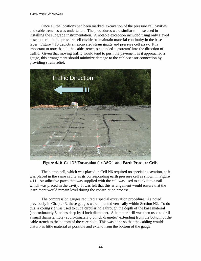
Once all the locations had been marked, excavation of the pressure cell cavities and cable trenches was undertaken. The procedures were similar to those used in installing the subgrade instrumentation. A notable exception included using only sieved base material in the pressure cell cavities to maintain material continuity in the base layer. Figure 4.10 depicts an excavated strain gauge and pressure cell array. It is important to note that all the cable trenches extended ‘upstream’ into the direction of traffic. Given that moving traffic would tend to push the pavement as it approached a gauge, this arrangement should minimize damage to the cable/sensor connection by providing strain relief.

Figure 4.10 Cell N8 Excavation for ASG’s and Earth Pressure Cells.

The button cell, which was placed in Cell N6 required no special excavation, as it was placed in the same cavity as its corresponding earth pressure cell as shown in Figure 4.11. An adhesive patch that was supplied with the cell was used to stick it to a nail which was placed in the cavity. It was felt that this arrangement would ensure that the instrument would remain level during the construction process. The compression gauges required a special excavation procedure. As noted previously in Chapter 3, these gauges were mounted vertically within Section N2. To do this, a coring rig was used to cut a circular hole through the depth of the base material (approximately 6 inches deep by 4 inch diameter). A hammer drill was then used to drill a small diameter hole (approximately 0.5 inch diameter) extending from the bottom of the cable trench to the bottom of the core hole. This was done so that the cabling would disturb as little material as possible and extend from the bottom of the gauge.

Traffic Direction


45

Figure 4.11 Placement of Button Cell in Section N6.

Gauge Installation Once each cable and gauge excavation had been made, the sensors were installed prior to paving. While each of the sensor types will be discussed separately below, they were installed as a group by section to facilitate construction. Base Earth Pressure Cells and Button Cell The earth pressure cells installed in the top of the base layer followed essentially the same procedure as outlined previously in the discussion of the subgrade earth pressure cells. However, rather than mound base material on top of the gauge for protection, hot-mix that had been raked to remove large particles was placed just prior to paving. The contractor dumped hot mix on the inside lane, which was raked with a lute and carried by shovel to the pressure cell location. It was then placed on top of the pressure cell, spread by hand and compacted using a trowel and wooden tamping plate. The button cell in N6 was included in this process.

N6 Earth Pressure Cell

Button Cell

Button Cell Cable


46

Asphalt Strain Gauges Prior to placement of the ASG’s, -#8 granular base material was placed to a depth of 1 in. in each of the 3 inch deep cable trenches. The gauges were then placed in their rough location with proper orientation (transverse or longitudinal) and the cables were laid in the trenches. The trenches were then filled with the same sieved material and compacted using a Marshall hammer to restore the grade. Portions of this procedure are depicted in Figure 4.12.

Figure 4.12 Approximate Placement of ASGs.

It must be noted that in placing the first array of strain gauges (Section N3), there were a number of gauges that either did not have a cable tie anchoring the cable to axial bar or it was removed to facilitate placement of the cable in the trench. One such gauge is depicted in Figure 4.13. Immediately after paving, approximately half (six) of the twelve gauges were not functioning in Section N3. Whether this was a contributing factor to the poor survivability of gauges in Section N3 is difficult to determine since the gauges are not able to be recovered without damaging both the gauge and the pavement. However, in each of the successive gauge arrays, cable ties were used to attach the cable to the axial bar and transverse flange of each instrument in an attempt to provide strain relief to the connection. This is shown in Figure 4.14. In general, survivability


47

immediately after paving of the ASG’s improved in each of the other seven test sections. A full discussion of gauge survivability is provided at the end of this chapter.

Figure 4.13 ASG with Cable Tie Missing from Axial Bar.

Figure 4.14 ASG with Additional Cable Ties.

After the gauges had been placed in their approximate locations as shown in Figure 4.15, and the contractor was ready to pave, a sand/asphalt mix was prepared to adhere the ASG’s to the base material. The sand/asphalt mix used a -#10 sand mixed with PG 76-22 at a 1:2 binder:sand ratio. The mixture was heated and placed, approximately 1/8” thick by spatula in the shape of the ASG’s. The gauges were then gently pushed down into the mix and properly oriented (transverse or longitudinal). This procedure is depicted in Figure 4.16.

Cable Ties


48

Figure 4.15 Gauge Layout Prior to Paving.

a) Placing Sand/Asphalt Mix b) Finished Gauge Figure 4.16 Placing Sand/Asphalt Mix Just Prior to Paving.

Once all the gauges in an array had been adhered using the sand/asphalt mix, HMA that had been hand raked to remove large particles was placed by hand on top of each gauge, spread and compacted using a trowel and wooden compacting plate (1 ft x 1 ft). The material was placed so that no part of the gauge was exposed, resulting in approximately 1.25” of cover material. This procedure is depicted in Figure 4.17.


49

Figure 4.17 Placing Cover Material on ASGs.

After the cover material was placed, and the paver had been lined up to straddle the gauge array (Figure 4.18), the respective sections were paved. During paving the gauges were monitored for survivability and response (Figure 4.19). It was due to monitoring that the changes to the cable ties, noted above, were made after paving the first section (N3). As discussed in Chapter 3, ASG’s were also placed on top of the bottom lift in Sections N7 and N8. The installation procedure here was essentially the same as the previous installation, however no cable trenches were dug. Instead, the cables were simply adhered to the existing hot mix layer with the sand/binder mix. Figure 4.20 illustrates this process which included placing cover material over all exposed cables. This was done to prevent severing of the cables by the paver wheels.


50

Figure 4.18 Paver Straddling Gauge Array.

Figure 4.19 Monitoring Gauges During Construction.


51

a) Adhered ASG

b) Tacking Gauge Cables

c) Covered Gauges and Cables Figure 4.20 Installation of ASG's on Top of First Hot Mix Lift (Section N7).

Vertical Compression Gauges The excavation process for the vertical compression gauges was described above. To place the gauges, the gauge cables were first strung through the cable holes extending from the bottom of the hole to the cable trench as shown schematically in Figure 4.21. Sieved base material was then mixed with enough water to make it cohesive and enable it to be packed around the gauge. The gauge was then placed inside the hole and additional material was packed along the sides. One concern with this installation is that no rigorous compaction could be employed so it may represent an area of unusually low density.


52

Figure 4.21 Vertical Compression Gauge Installation.

TEMPERATURE PROBES The temperature probes were the last gauges to be installed at the test track and were installed after paving had been completed. A completed installation is shown in Figure 4.22. The installation process followed these steps:

1. A hole was drilled slightly larger than the diameter of the gauge array vertically into the pavement. The hole extended approximately 10.5” deep and was just outside the white edge stripe of the pavement.

2. A v-notch approximately ¾” deep was cut from the hole to the edge of the pavement to serve as a cable trench.

3. The gauge was covered with a rubberized asphalt joint and crack filler commonly available at home improvement stores.

4. The hole was filled with the same rubberized asphalt material. 5. The temperature gauge array was then inserted into the hole so that the top gauge

was just below the surface and worked around to ensure no air pockets would be present.

6. Particles from the v-notch were broken up and seated on top of the rubberized material to simulate the surrounding pavement surface.

7. The cable was laid in the v-notch trench and covered with a cold patch material commonly available at home improvement stores.

Vertical Compression Gauge Sieved Granular Base Material with Added Moisture During Installation

Drilled Cable Hole

Sensor Cable


53

Figure 4.22 Completed Temperature Probe Installation.

GAUGE MONITORING DURING CONSTRUCTION AND SURVIVABILITY Throughout the construction process, the gauges were monitored through several means which was discussed, in part, above. The main purpose for this was to evaluate if the construction activities were compromising the instrumentation so that changes could be made during the process to improve survivability. The main issue during construction was whether to use vibratory compaction while over the gauge array during the process since the gauge manufacturers recommended against vibration. However, there was concern of project members that eliminating vibratory rolling could result in unrepresentative densities in the region near the gauges. Therefore, it was decided to try the first section with compaction proceeding according to the contractor’s protocol. Full details regarding the construction practices can be found in (Powell, 2004). Based on field observations it did not appear that using vibration was the cause of gauge failure. In other words, though some gauges did fail, it was not widespread and therefore normal compaction procedures were used throughout the construction process. Once the high speed data collection began, it was possible to determine which gauges had fully survived the installation process. However, without extracting the gauges and performing forensic studies, it is impossible to precisely define why the gauges failed. Table 4.1 summarizes the gauge performance, as of November 7, 2003, for the asphalt strain gauges and earth pressure cells. Tables 4.1 through 4.8 are more detailed and list whether each gauge is currently functioning, behaving erratically under load, exhibiting excessive noise, or not responding. An example of each type of behavior is shown in Figures 4.23 through 4.26. As shown in Table 4.1, the earth pressure cells are at 100% survivability. To date, there do not appear to be any problems with any of these gauges. The asphalt strain gauges, however, had nearly 1 in 4 gauges not responding under load. This number may be artificially high since it has been observed through examining the slow speed data that some gauges will drift on and off scale with temperature. This phenomenon is currently

Lane Edge Stripe

Top of Temp Gauge BundleV-notch with

Buried Cables


54

under investigation and may be dealt with through using a precision resistor or acquiring a signal conditioning card with a wider full scale range. At the time this report was prepared, these gauges were under observation. It must be noted that it was expected that the asphalt strain gauges would have a poorer survivability rate. This explains the redundancy of gauges placed in the same relative locations with respect to the wheel path. With that in mind, there were essentially six strain measurements desired in each section (3 transverse and 3 longitudinal in the center, to the right and to the left of the wheelpath) totaling 48 locations. With consideration of redundancy, 39 of 48 (81.3%) locations are currently functioning which is certainly better than the 65.2% overall noted in Table 4.1. Table 4.1 Asphalt Strain Gauge and Earth Pressure Cell Survivability.

Gauge Type Asphalt Strain

Gauge Earth Pressure Cell Functional 65.2% 100.0%

Erratic 8.9% 0.0% Noisy 1.8% 0.0%

No Response 24.1% 0.0%


55

Table 4.2 Section N1 Survivability. Sensor Gauge Status

N1OSBLR Functional

N1OSBTR Erratic Under Load

N1OSBLC Functional

N1OSBTC Functional

N1OSBLL No Response

N1OSBTL Functional

N1OSALR Functional

N1OSATR Erratic Under Load

N1OSALC Functional

N1OSATC Functional

N1OSALL Functional

N1OSATL Erratic Under Load

N10PASC Functional

N1OPBBC Functional

%No Response 7.1% %Erratic Under Load 21.4%

%Noisy 0.0% %Functional 71.4%


56

Table 4.3 Section N2 Survivability. Sensor Comments

N2OSBLR Functional

N2OSBTR Functional

N2OSBLC Functional

N2OSBTC No Response

N2OSBLL Functional

N2OSBTL No Response

N2OSALR Functional

N2OSATR Functional

N2OSALC Functional

N2OSATC Functional

N2OSALL Functional

N2OSATL Functional

N20PASC Functional

N2OPBBC Functional

Inside Comp Noisy Signal

Outside Comp Noisy Signal


%Noisy 12.5% % Functional 75.0%


57


N3OSBLR Functional

N3OSBTR No Response

N3OSBLC Functional

N3OSBTC No Response

N3OSBLL No Response

N3OSBTL Erratic Under Load

N3OSALR No Response

N3OSATR No Response

N3OSALC No Response

N3OSATC No Response

N3OSALL Functional

N3OSATL No Response

N30PASC Functional

N3OPBBC Functional


% Noisy 0.0% % Functional 35.7%


58


N4OSBLR Functional

N4OSBTR Functional

N4OSBLC Functional

N4OSBTC Functional

N4OSBLL No Response

N4OSBTL Noisy Signal

N4OSALR Functional

N4OSATR Functional

N4OSALC No Response

N4OSATC Erratic Under Load

N4OSALL Functional

N4OSATL No Response

N40PASC Functional

N4OPBBC Functional




59


N5OSBLR Erratic Under Load

N5OSBTR No Response

N5OSBLC Functional

N5OSBTC No Response

N5OSBLL Functional

N5OSBTL Functional

N5OSALR Functional

N5OSATR Noisy Signal

N5OSALC No Response

N5OSATC No Response

N5OSALL Erratic Under Load

N5OSATL Functional

N50PASC Functional

N5OPBBC Functional




60


N6OSBLR Functional

N6OSBTR Functional

N6OSBLC Functional

N6OSBTC Erratic Under Load

N6OSBLL Functional

N6OSBTL Functional

N6OSALR Functional

N6OSATR Functional

N6OSALC Functional

N6OSATC Functional

N6OSALL No Response

N6OSATL Functional

N60PASC Functional

N6OPBBC Functional

Button Cell Noisy Signal




61


N7OSBLR Functional

N7OSBTR Functional

N7OSBLC Functional

N7OSBTC Functional

N7OSBLL Functional

N7OSBTL Functional

N7OSALR Functional

N7OSATR Functional

N7OSALC Functional

N7OSATC Functional

N7OSALL Functional

N7OSATL No Response

N7OPASC Functional

N7OPBBC Functional

N7IPASC Functional

N7IPBBC Functional

N7OSBLC2 No Response

N7OSBTC2 Functional

N7OSATC2 No Response

N7OSALC2 Functional




62


N8OSBLR Functional

N8OSBTR Functional

N8OSBLC Functional

N8OSBTC Erratic Under Load

N8OSBLL No Response

N8OSBTL Functional

N8OSALR Functional

N8OSATR No Response

N8OSALC Functional

N8OSATC Erratic Under Load

N8OSALL No Response

N8OSATL No Response

N80PASC Functional

N8OPBBC Functional

N8OSBLC2 No Response

N8OSBTC2 Functional

N8ISBLC2 Functional

N8ISBTC2 Functional

N8ISBLC Functional

N8ISBTC Functional

N8ISBLL Functional

N8ISBTL Functional

N8ISALC Functional

N8ISATC Functional

N8ISALL Functional

N8ISATL Functional

%No Response 19.2%

%Erratic Under Load 7.7%

%Noisy 0.0%

% Functional 73.1%


63

2.4 2.6 2.8 3 3.2 3.4 3.6 3.8 4 4.2 4.4

-3

-2.5

-2

-1.5

-1

W 1: Cha nne l 1

Figure 4.23 An Example of a Functioning Sensor Under Traffic.

2 .4 2 .6 2 .8 3 3 .2 3 .4 3 .6 3 .8 4 4 .2 4 .4 4 .6 4 .8

- 2

0

2

4

W 8 : C h a n n e l 8

Figure 4.24 An Example of a Sensor Behaving Erratically Under Traffic.


64

0 1 2 3 4 5 6 7 8- 3 .0 2

- 3 .0 1

- 3

- 2 .9 9

- 2 .9 8

- 2 .9 7

- 2 .9 6

- 2 .9 5 W 1 5 : C h a n n e l 1 5

Figure 4.25 An Example of a Sensor Exhibiting Excessive Noise.

0 1 2 3 4 5 6 7 8- 1 0

- 8

- 6

- 4

- 2

0 W 6 : C h a n n e l 6

Figure 4.26 An Example of a Sensor Not Responding Under Load.

SUMMARY This chapter detailed the installation procedures used to instrument test sections N1 through N8 at the test track. Generally speaking, the final installation procedures used at the track were viewed as successful, though a key modification of adding cable ties to the asphalt strain gauges seemed to improve the survivability rate of these devices. In the future, as data are gathered from these gauges, a better assessment of the installation procedures can be made. Additionally, there may be an opportunity to perform forensic studies on the gauges themselves.


65

CHAPTER 5 - SUMMARY, CONCLUSIONS AND RECOMMENDATIONS

This report detailed the design and instrumentation of a structural experiment at the NCAT test track. The objectives of this experiment include:

1. Validating mechanistic pavement models for flexible pavements. 2. Developing transfer functions for typical asphalt mixtures and pavement cross-

sections used in Alabama. 3. Studying dynamic effects on pavement deterioration from a mechanistic

viewpoint. 4. Evaluating the effect of thickness and polymer modification on structural

performance. To accomplish these objectives, eight sections were built at the NCAT test track consisting primarily of three HMA thicknesses and modified versus unmodified binders. Additionally, two sections were devoted to having an SMA surface course and a rich bottom layer. Each of the test sections was instrumented with moisture, temperature, strain and pressure gauges to measure pavement responses under traffic and environmental loading. Sensor selection, calibration and basic operating principles were discussed. Additionally, details regarding the data acquisition systems were provided. The installation procedures were documented. While the asphalt strain gauge procedures were deemed effective (85% of strain gauge locations are functional), it is recommended that in future installations additional cable ties be added to the asphalt strain gauges. The procedures used for the earth pressure cells resulted in 100% survivability at the writing of this report. As planning begins for the 2006 research cycle, where there may be more sections devoted to instrumentation, the following recommendations are made: 1. Investigate high-speed wireless data collection and transmission. The current high-

speed collection scheme requires personnel beside the track while trucks are operating. A safer mode of operation would not have personnel near the track. Also, it is likely that many more sections would require a high-speed datalogger for each section. A wireless system to collect and transmit these data would certainly facilitate data collection.

2. Continue to investigate gauge technology as many advances may be made in the coming two years that could greatly improve survivability and the ability to measure in situ pavement responses.

3. Conduct an external field experiment to investigate the effects of installation on pavement density. The results of this experiment could further guide installation efforts during the next research cycle.


66

REFERENCES 1. --, “Minnesota Road Research Project, Work Plan for Research Objectives,” Report

No. 90-03, Minnesota Department of Transportation, 1990.

2. Baker, H.B., Buth, M.R. and Van Deusen, D.A., “Minnesota Road Research Project Load Response Instrumentation Installation and Testing Procedures,” Report No. MN/PR-94/01, Minnesota Department of Transportation, St. Paul, MN, 1994.

3. E.R. Brown, L. Allen Cooley, Jr., Doug Hanson, Cynthia Lynn, Buzz Powell, Brian Prowell and Don Watson, “NCAT Test Track Design, Construction, and Performance,” Report No. 2002-12, National Center for Asphalt Technology, 2002.

4. Chadbourn, Bruce A., David E. Newcomb, and David H. Timm, “Measured and Theoretical Comparisons of Traffic Loads and Pavement Response Distributions,” Proceedings, Eighth International Conference on Asphalt Pavements, Seattle, WA, 1997, pp. 229-238.

5. Epps, J; Monismith, CL; Seeds, SB; Alavi, SH; Ashmore, SC; Leahy, R; Mitchell, TM, “Performance of HMA Test Sections at WESTRACK,” Journal of the Association of Asphalt Paving Technologists, Vol. 67, 1998, pp. 738-782.

6. Freeman, Reed B., H. Tommy Carr, Tom McEwen, and R. Buzz Powell, “Instrumentation at the National Center for Asphalt Technology Test Track.” U.S. Army Corps of Engineers, Engineer Research and Development Center, Report No. ERDC TR-01-9. Washington, D.C. August 2001.

7. HRB, “Report of Committee on Classification of Materials for Subgrades and Granular Type Roads,” Proceedings, Highway Research Board, Vol. 25, 1945, pp. 376-384.

8. HRB, “The AASHO Road Test,” Report 5, Highway Research Board, 1962.

9. Huang, Y.H., Pavement Design and Analysis, Second Edition, Pearson Prentice Hall, 2004.

10. Jess, J., “Determination of Structural Coefficients for New HMA Mixtures,” M.S. Thesis, Auburn University, 2004.

11. Loulizi, A; Al-Qadi, IL; Lahouar, S; Freeman, TE, “Data Collection and Management of the Instrumented Smart Road Flexible Pavement Sections,” Transportation Research Record No. 1769, Transportation Research Board, 2001, pp. 142-151.

12. National Cooperative Highway Research Program, http://www.2002designguide.com/, NCHRP Project 1-37A, accessed Dec. 1, 2003.


67

13. Newcomb, D.E., A.A. Bu-bushait, J.P. Mahoney and J. Sharma. State-of-the-Art on Pavement Overlay Design Procedures, Vol. 1. Report No. WA-RD 65.1, Washington State Department of Transportation, Olympia, Washington, 1983.

14. Office of Materials and Road Research, Minnesota Department of Transportation, http://www.mrr.dot.state.mn.us/research/MnROAD_Project/MnROADProject.asp, accessed Dec. 1, 2003.

15. Powell, R. Buzz, “As-Built Properties of Experimental Sections on the 2003 NCAT Pavement Test Track,” National Center for Asphalt Technology, 2004.

16. Smart Road Pavement Research Team, http://www.cee.vt.edu/program_areas/tise/smart/, accessed December 1, 2003.

17. Timm, D.H. and Newcomb, D.E., “Calibration of Flexible Pavement Performance Equations,” Transportation Research Record, Transportation Research Board, Accepted for Publication, 2003 (in press).

18. Timm, D.H., Birgisson, B. and Newcomb, D.E., “Weslea for Windows 3.0”, 1999,

available for download at: www.eng.auburn/edu/users/timmdav/WFW.msi.

19. Van Cauwelaert, F.J., Alexander, D.R., White, T.D., and Barker, W.R., “Multilayer Elastic Program for Backcalculating Layer Moduli in Pavement Evaluation,” Nondestructive Testing of Pavements and Backcalculation of Moduli, ASTM STP 1026, A.J. Bush III and G.Y. Baladi, Eds., American Society for Testing and Materials, Philadelphia, 1989, pp. 171-188.


68

APPENDIX A

Instrumentation Data Sheets


69


70


71

This compact transducer measures 6.5mm in diameter and 1m in thickness, andcan be used safel in water. It is suitable for various modeling tests incivil engineering.

-- Specifications --

Type PDA-200KPA PDB-200KPA

PDA-500KPA PDB-500KPA

PDA-1MPA PDB-1MPA

Capacity 200kPa 500kPa 1 MPa Rated Output* 0.8mV/V 1mV/V Non-linearity 1%RO Hysteresis 1%RO Temperature Range Allowable -20 to +70°C Resistance 350 ohm Exciting Voltage Recommended Less than 2V Electrical Connection 0.005mm2 4-core Fluoride plastic insulated Cable 2m Weight PDA-PA: 0.1g /PDB-PA: 0.5g

*Rated Output:1mV/V=2000x10-6strain


72

PDA-PA PDB-PA

Source: http://www.tokyosokki.co.jp/e/product/transducer/pressure/detail/pda-pa.html


73

APPENDIX B

High Speed Data Acquistion – Channel Assignments


74

Table B.1 Section N1 High Speed Data Channel Assignments. Channel Sensor

A1 N1OSBLR

A2 N1OSBTR

A3 N1OSBLC

A4 N1OSBTC

A5 N1OSBLL

A6 N1OSBTL

A7 N1OSALR

A8 N1OSATR

A9 N1OSALC

A10 N1OSATC

A11 N1OSALL

A12 N1OSATL

A13 N1OPASC

A14 N1OPBBC


75

Table B.2 Section N2 High Speed Data Channel Assignments.

Channel Sensor A1 N2OSBLR

A2 N2OSBTR

A3 N2OSBLC

A4 N2OSBTC

A5 N2OSBLL

A6 N2OSBTL

A7 N2OSALR

A8 N2OSATR

A9 N2OSALC

A10 N2OSATC

A11 N2OSALL

A12 N2OSATL

A13 N2OPASC

A14 N2OPBBC

A18 Inside Compression

A19 Outside Compression


76


A1 N3OSBLR

A2 N3OSBTR

A3 N3OSBLC

A4 N3OSBTC

A5 N3OSBLL

A6 N3OSBTL

A7 N3OSALR

A8 N3OSATR

A9 N3OSALC

A10 N3OSATC

A11 N3OSALL

A12 N3OSATL

A13 N3OPASC

A14 N3OPBBC


77


A1 N4OSBLR

A2 N4OSBTR

A3 N4OSBLC

A4 N4OSBTC

A5 N4OSBLL

A6 N4OSBTL

A7 N4OSALR

A8 N4OSATR

A9 N4OSALC

A10 N4OSATC

A11 N4OSALL

A12 N4OSATL

A13 N4OPASC

A14 N4OPBBC


78


A1 N5OSBLR

A2 N5OSBTR

A3 N5OSBLC

A4 N5OSBTC

A5 N5OSBLL

A6 N5OSBTL

A7 N5OSALR

A8 N5OSATR

A9 N5OSALC

A10 N5OSATC

A11 N5OSALL

A12 N5OSATL

A13 N5OPASC

A14 N5OPBBC


79


A1 N6OSBLR

A2 N6OSBTR

A3 N6OSBLC

A4 N6OSBTC

A5 N6OSBLL

A6 N6OSBTL

A7 N6OSALR

A8 N6OSATR

A9 N6OSALC

A10 N6OSATC

A11 N6OSALL

A12 N6OSATL

A13 N6OPASC

A14 N6OPBBC

A17 Button Cell


80


A1 N7OSBLR A2 N7OSBTR A3 N7OSBLC A4 N7OSBTC A5 N7OSBLL A6 N7OSBTL A7 N7OSALR A8 N7OSATR A9 N7OSALC A10 N7OSATC A11 N7OSALL A12 N7OSATL A13 N7OPASC A14 N7OPBBC A15 N7IPASC A16 N7IPBBC A21 N7OSBLC2 A22 N7OSBTC2 A23 N7OSATC2 A24 N7OSALC2


81


A1 N8OSBLR A2 N8OSBTR A3 N8OSBLC A4 N8OSBTC A5 N8OSBLL A6 N8OSBTL A7 N8OSALR A8 N8OSATR A9 N8OSALC

A10 N8OSATC A11 N8OSALL A12 N8OSATL A13 N8OPASC A14 N8OPBBC A21 N8OSBLC2 A22 N8OSBTC2 A23 N8ISBLC2 A24 N8ISBTC2 A25 N8ISBLC A26 N8ISBTC A27 N8ISBLL A28 N8ISBTL A29 N8ISALC A30 N8ISATC A31 N8ISALL A32 N8ISATL

Date post:	20-Aug-2018
Category:	Documents
Upload:	danghuong
View:	214 times
Download:	0 times

DESIGN AND INSTRUMENTATION OF THE STRUCTURAL PAVEMENT ... Reports/04-01 Design and... · DESIGN AND...

Documents