DESIGN AND OPTIMIZATION OF DATA ACQUISITION SYSTEM …

DESIGN AND OPTIMIZATION OF DATA ACQUISITION SYSTEM USING

WIRELESS UNDERGROUND SENSOR NETWORKS

by

Raghu Krishnappa, M.Tech

A thesis submitted to the Graduate Council of

Texas State University in partial fulfillment

of the requirements for the degree of

Master of Science

with a Major in Engineering

December 2017

Committee Members:

Semih Aslan

Harold Stern

Karl Stephan

George Koutitas

Bahram Asiabanpour

COPYRIGHT

by

Raghu Krishnappa

FAIR USE AND AUTHOR’S PERMISSION STATEMENT

Fair Use

This work is protected by the Copyright Laws of the United States (Public Law 94-553,

section 107). Consistent with fair use as defined in the Copyright Laws, brief quotations

from this material are allowed with proper acknowledgment. Use of this material for

financial gain without the author’s express written permission is not allowed.

Duplication Permission

As the copyright holder of this work, I, Raghu Krishnappa, authorize duplication of this

work, in whole or in part, for educational or scholarly purposes only.

DEDICATION

To my family,

for their endless love and support

v

ACKNOWLEDGEMENTS

I would like to express my sincere thanks to my advisor Dr. Semih Aslan for

giving me the opportunity to work with him, and for his guidance, support, and

encouragement during my entire MS program. I am grateful to him for his trust,

patience, and constructive criticisms, which helped me improve the quality of my

research. Dr. Aslan not only trained me to be a good student, but he has also taught

me in many other ways that could lead me to success in my future career.

I wish to express my gratitude to all the faculty members of the Ingram School

of Engineering at Texas State University for their excellent advice, constructive

criticism, and helpful and critical reviews throughout my MS program. A special

thank, goes to Harold Stern, Karl Stephan, Bahram Asiabanpour, and George Koutitas,

who kindly agreed to serve in my thesis defense committee. Their valuable comments

and enlightening suggestions have helped me to achieve a stable research path towards

this thesis.

I would also like to thank all my friends for creating a wonderful family-like

atmosphere and giving me a warm memory during my MS student life. Finally, I would

like to express my sincere gratitude to my parents, for their patience, continuous

support and encouragement throughout this thesis. Special thanks to my friend

Mahima Sajan Varghese for her constant support and valuable suggestions throughout

my research.

vi

TABLE OF CONTENTS

ACKNOWLEDGEMENTS ........................................................................................... v

LIST OF TABLES ......................................................................................................viii

LIST OF FIGURES ...................................................................................................... ix

LIST OF ABBREVIATIONS ...................................................................................... xii

ABSTRACT ................................................................................................................xiii

CHAPTER

1. INTRODUCTION .................................................................................................. 1

1.1. Background .................................................................................................. 1

1.2. EM Wave Based WUSNs in Soil Medium .................................................. 5

1.3. Research Objectives and Solutions.............................................................. 6

1.4. Thesis Outline .............................................................................................. 7

2. LITERATURE REVIEW ....................................................................................... 8

2.1. Previous Work Related to WUSN ............................................................... 8

2.2. Frequency Band Selection ........................................................................... 9

2.3. Antenna Design ......................................................................................... 10

3. PROPOSED SYSTEM ......................................................................................... 12

3.1. Subsurface Subsystem ............................................................................... 14

3.2. Surface System .......................................................................................... 16

3.3. Sensors ....................................................................................................... 17

3.4. Analog to Digital Converter ...................................................................... 18

3.5. Raspberry Pi .............................................................................................. 20

3.6. Hack RF One ............................................................................................. 20

3.7. Power Usage and Battery .......................................................................... 22

vii

4. DESIGN AND DEVELOPMENT OF WIRELESS UNDERGROUND SENSOR

NETWORK FOR PIPELINE MONITORING ............................................................ 25

4.1. GNU Radio ................................................................................................ 26

4.2. Modulation Scheme ................................................................................... 27

4.3. Antenna Design Parameters....................................................................... 30

4.4. Antenna for 450 MHz ................................................................................ 34

4.5. Antenna for 900 MHz ................................................................................ 35

4.6. Channel Model .......................................................................................... 38

4.7. Demodulation Scheme ............................................................................... 41

4.8. Data Display using HTML ........................................................................ 41

5. EXPERIMENT RESULTS................................................................................... 43

5.1. Sensor Data ................................................................................................ 43

5.2. GNU Radio Program ................................................................................. 44

5.3. Transmitted and Received Signal Analysis ............................................... 48

5.4. HTML display ........................................................................................... 58

6. CONCLUSION .................................................................................................... 59

APPENDIX .................................................................................................................. 60

REFERENCE ............................................................................................................. 101

viii

LIST OF TABLES

TABLE PAGE

Table I: Raspberry Pi power consumption................................................................... 24

Table II: Radiating field of different antennas ............................................................. 33

Table III: Antenna design specifications ..................................................................... 33

Table IV: 450MHz receiver antenna specifications..................................................... 34

Table V: 450MHz transmitter antenna specifications ................................................. 35

Table VI: 900MHz receiver antenna specifications..................................................... 36

Table VII: 900MHz transmitter antenna specifications ............................................... 37

Table VIII: Data transmission analysis ........................................................................ 56

ix

LIST OF FIGURES

FIGURE PAGE

Figure 1: Block diagram of Wireless Underground Sensor Network ........................... 3

Figure 2: Experimental Setup of proposed system ...................................................... 13

Figure 3: Subsurface system block diagram ................................................................ 15

Figure 4: Soil, Clay and sand arrangement in container .............................................. 15

Figure 5: Subsurface experimental setup ..................................................................... 16

Figure 6: Surface subsystem ........................................................................................ 17

Figure 7: Raspberry Pi 3 to MCP 3008 wiring diagram .............................................. 18

Figure 8: Analog to Digital Converter (ADC) MCP 3008 pin details ......................... 19

Figure 9: Hack RF One hardware (SDR) ..................................................................... 21

Figure 10: Power usage measurement setup ................................................................ 24

Figure 11: Signal processing and Data Acquisition System ........................................ 25

Figure 12: Software Defined Radio (SDR) block diagram .......................................... 26

Figure 13: GNU Radio components ............................................................................ 27

Figure 14: QPSK modulator ........................................................................................ 29

Figure 15: Constellation diagram of QPSK ................................................................. 29

Figure 16: Radiation pattern of isotropic antenna........................................................ 31

Figure 17: Radiation pattern of directional antenna .................................................... 31

x

Figure 18: Radiation patterns of antennas in the proposed system .............................. 32

Figure 19: Radiation pattern of 900-MHz parabolic antenna ..................................... 37

Figure 20: Radiation pattern of 900MHz ceiling mount antenna ................................ 38

Figure 21: Path loss with respect to distance ............................................................... 40

Figure 22: QPSK demodulator..................................................................................... 41

Figure 23: HTML display of sensor data ..................................................................... 42

Figure 24: Raw sensor data read by a terminal python program. ................................ 43

Figure 25: Raw sensor data saved in .csv format......................................................... 44

Figure 26: GNU Radio program for modulation and transmission ............................. 46

Figure 27: GNU Radio program at reception and demodulation ................................. 47

Figure 28: FFT plot of transmitted signal at 450MHz ................................................. 48

Figure 29: Spectrum analyser output of received signal at 450MHz........................... 49

Figure 30: Constellation plot of transmitted signal at 450 MHz ................................. 50

Figure 31: Constellation plot of received signal at 450 MHz ...................................... 50

Figure 32: Waterfall diagram of transmitted signal at 450MHz ................................. 51

Figure 33: Waterfall diagram of received signal at 450MHz ..................................... 51

Figure 34: Waterfall diagram of transmitted signal at 900MHz .................................. 52

Figure 35: Waterfall diagram of received signal at 900MHz ..................................... 52

Figure 36: Signal scope of transmitted signal a 900 MHz ........................................... 53

xi

Figure 37: Signal scope of received signal at 900 MHz .............................................. 53

Figure 38: Signal scope of received signal .................................................................. 54

Figure 39: Experimental testbed for calculating data rate and SNR ............................ 55

Figure 40: Displaying the received data in HTML page ............................................. 58

xii

LIST OF ABBREVIATIONS

Abbreviation Description

ADC Analog to Digital Converter

ASK Amplitude Shift Keying

DAQ Data Acquisition System

EM Electro-Magnetic

FSK Frequency Shift Keying

HMTL Hypertext Markup Language

PSK Phase Shift Modulation

QAM Quadrature Amplitude Modulation

QPSK Quadrature Phase Shift Keying

RF Radio Frequency

SDR Software Defined Radio

SPI Serial Peripheral Interface

TTE Through-The-Earth

WSN Wireless Sensor Network

WUSN Wireless Underground Sensor Network

xiii

ABSTRACT

The growth of Wireless Underground Sensor Networks (WUSN) will lead to

numerous emerging applications, such as underground pipelines, oil reservoir

monitoring, intelligent agriculture, earthquake and landslide forecasting, border patrol,

underground mine disaster prevention, and rescue. Underground environments prevent

the use of most current wireless communication and networking systems, due to its

extremely high attenuation to the propogation of signals, small communication range,

and high dynamics of electromagnetic (EM) waves when penetrating through soil, rock,

sand, water, crude oil medium and other underground environments. The objective of

this research is to address these unique and significant challenges for the realization of

wireless sensor networks in underground data monitoring systems. Research also

focuses on developing a general framework using underground wireless sensor

networks to provide continuous monitoring of pipeline to detect water leakage.

1

1. INTRODUCTION

1.1. Background

The application of Wireless Sensor Network (WSN) for remote data acquisition and

monitoring is not limited to terrestrial applications. WSN technology can be extended

underground where applications include agriculture, security, and infrastructure

monitoring. Wireless Underground Sensor Networks (WUSN) has the most favorable

applications in the recent development of Wireless Network Sensor technology. WUSN is

a special WSN that concentrate on burying the Data Acquisition System(DAQ) along with

sensors in the subsurface of the soil at depths that can range from few a meters to hundreds

of meters from the top surface of soil usually targeting agriculture, structural health

monitoring, border patrol, sports field maintenance, environment monitoring, and

improving the performance of various distribution infrastructures to reduce the waste of

resources [1-10].

The main difference between WSNs and WUSNs is the communication channel.

The difference between wave propagation of Electromagnetic(EM) waves in air and soil is

so significant that the empherical model of the wireless channel in soil has only been

available in recent years. Despite its advantages, many problems exist that makes it difficult

to build a WUSN system. The challenge is the realization of reliable and efficient

underground wireless communication between the buried system and surface Data

Acquisition System (DAQ). Many factors such as temperature, soil moisture, weather, soil

composition, and homogeneity impact the communication and connectivity. In addition to

2

these factors, the operating frequency of the electromagnetic (EM) wave and the burial

depth have a substantial effect on the communication.

In this research, a detailed analysis of WUSNs was done, and a robust model that

can operate at high frequencies was developed, which can perform better than the existing

models that operate at low operating frequency. The block diagram of the system is shown

in Figure 1. The sensors along with the signal processing unit and the antenna were buried

at a distance of 2-6 meters from the soil surface. The measurement system includes

parameters like temperature, humidity, soil sensor output, and moisture content. The

measurements were then processed and transmitted through the soil to the surface antenna.

This type of transmission is called “Through-The-Earth (TTE) communication.” The

measurements were stored and processed in the surface subsystem to make necessary

decisions. With each new generation of electronics, sensors have become smaller, less

expensive, lower power and more sophisticated, giving them the capability to produce

more and more data, which in turn allows more comprehensive assessment of an

ecosystem, more advanced warning of environmental threats, and more accurate (and

earlier) sensing of infrastructure problems. Buried sensors, however, have one common

problem – the difficulty of transmitting the sensed information to the surface. Typical radio

frequency data transmission systems (Bluetooth, WI-Fi, Cellular, etc.) do not work well

due to the difficulty of propagating Radio Frequency (RF), signal through the soil. A

system that could accurately and reliably transmit digital data from sensors buried 2 – 6

meters below ground to an above-ground receiver, at high speed and with low transmitter

power, would enable many new ecologically-based applications involving buried sensors.

3

Figure 1: Block diagram of Wireless Underground Sensor Network

Wireless Underground Sensor Networks (WUSNs) [11] are networks of wireless

sensor nodes operating below the earth surface. As an extension to the established wireless

sensor networks (WSNs) [12], WUSNs are used to provide real-time monitoring abilities

in two types of underground situations: tunnels and soil media. Constructed on the

monitored situations, the WUSNs can be further divided into two categories: the WUSNs

in underground mines and tunnels and the WUSNs in a soil medium. Related to current

underground monitoring strategies, WUSNs provide benefits in ease of deployment and

data collection, timeliness of data, coverage density, concealment, and reliability [11]. A

wide variety of novel and needed applications are empowered by WUSNs [2, 8, 11]

including:

4

Border Patrol and Intruder Detection: Border patrol is vital for national safety. The

conventional border patrol methods suffer from rigorous human participation. WUSNs

deployed alongside the border deliver a low cost, concealed, and reliable way to spot the

intruders crossing the border.

Landslide and Earthquake Monitoring: Until now, landslides and earthquakes have been

difficult to be precisely forecast. WUSNs deliver us a unique method to screen the signs of

landslide and earthquake in real time with minor organization and maintenance price tags.

As a result, the property loss and personal injury triggered by those unexpected tragedies

can be reduced.

Underground and Power Grid Monitoring: Pipelines constitute one of the most significant

methods to transport high volumes of liquid (e.g., water and oil) over elongated distances.

Yet, present leakage detection methods do not work well due to the harsh underground

environmental circumstances. Furthermore, in the existing underground power grid,

numerous errors, such as underground power grid fires triggered by overcapacity and cable

breakdown caused by careless tunneling, are hard to be localized, detected, avoided, and

fixed due to the unreachable environments. WUSNs can deliver real-time monitoring to aid

the proprietors to avoid the possible faults and repair existing errors in those underground

configurations.

Smart Irrigation: With the real-time monitoring of the temperature, soil moisture, and

other soil properties, the WUSNs can precisely define where and when to irrigate crops.

Assuming that the irrigation consumes more than 70% of fresh water all over the world

[13], the WUSNs can significantly improve the water sustainability.

5

Mine Disaster Rescue and Prevention: Existing techniques don’t support localization and

communications after disasters in mines, notably when an RF wireless channel is jammed

due to tunnel breakdowns and wired communication is nonfunctional due to the

breakdown of wires. Since a WUSN will be able to work in close underground locations,

it can significantly improve present mine productivity and safety.

Despite the advantages of WUSNs, the underground environment is an unfriendly

location for wireless communication and needs existing networking solutions, and

communication protocols for terrestrial WSNs to be reconsidered. Explicitly, the critical

difference between the WSNs and terrestrial WUSNs is the communication channel. To

deploy WUSNs in the underground, the propagation channel is no longer air but rock, soil,

metals, concrete, and water.

Even though the well-defined terrestrial signal propagation methods based on EM

waves may still work in the soil medium, the sole channel characteristics of EM waves in

this environment need to be remodeled. For the WUSNs installed in subway tunnels and

underground mines, the EM waves are appropriate for wireless signal transmission since

the radio signal propagates in air. However, the propagation properties of EM waves are

considerably different from the terrestrial wireless channels due to the limititations caused

by the ceilings and walls in mines and tunnels.

1.2. EM Wave Based WUSNs in Soil Medium

In the underground environment, the well-defined wireless communication systems

using electromagnetic waves do not work as expected [4]. EM waves experience

considerable propagation loss due to the absorption of rock, soil, and water in the

underground environment. Underground systems have limited power due to energy

6

restrictions; the transmission range is minimal. In addition, the path loss of EM waves in

the underground environment is dependent on many soil properties such as water content,

soil textures (clay, silt, or sand), and density. The soil properties can alter with time due to

surface weather and location. The transmission range of the underground communication

systems also differs dramatically in different locations and times.

In the proposed system of WUSNs in an underground environment, the underground

DAQ is expected to transmit sensed data to the surface subsystem. Hence, the connectivity

between buried subsurface system and the surface subsystem is essential for the system

functionalities. Due to the complex channel properties, the connectivity analysis in the

WUSNs is more complicated than that of the surface wireless sensor networks. The number

of underground sensors is limited due to the high installation and maintenance cost.

However, a very high-density underground sensor, is essential to reserve the full

connectivity of WUSNs due to harsh underground environment conditions.

1.3. Research Objectives and Solutions

The objective of the thesis is to investigate the distinctive characteristics of WUSNs

in underground environments and to discover the keys to realize efficient and reliable

communication in WUSNs. To evaluate WUSNs in the soil medium, we developed an

environment which imitates the soil transmission medium. To make it more realistic, a

Data Acquisition System (DAQ) along with transmitter was buried underground, and a

receiver and a laptop were used at the subsurface to read the sensor values and realize

underground water leakage detection and localization using WUSN. In this research, the

channel properties of EM waves in a soil environment are investigated specifically in the

400–900 MHz band which is better for the efficient communication compared to the 2.4

7

GHz or higher range. Antenna design and implementation of Quadrature Phase Shift

Keying (QPSK) in WUSN’s is an essential takeaway of this research.

1.4. Thesis Outline

This thesis is organized as follows. In Chapter 2, a detailed literature review based on

previous work related to WUSN is explained. In Chapter 3, the experimental setup and

hardware used in the subsurface subsystem and the surface subsystem is explained in detail.

In Chapter 4, detailed design and purpose of each device and software are explained. In

Chapter 5, results and analysis of results are explained. Finally, Chapter 6 summarizes the

overall research contributions and possible future research are mentioned.

8

2. LITERATURE REVIEW

2.1. Previous Work Related to WUSN

The concept of Wireless Underground Sensor Network’s was first presented in 2007

[4], after which many applications have been developed based on WUSNs. In [4], the

WUSN is used to acquire critical data in underground tunnels to provide a safe

environmental conditions in mines. In [5], the WUSNs are deployed during the fracturing

process in crude oil extraction, that measures many critical information about the

environment inside oil reservoirs. In [6, 7] the WUSNs are utilized to detect leakage in the

pipeline where Magnetic Induction (MI) communications were used for communication.

But [6, 7] have no limitation on power consumption which is critical in WUSNs. In a few

applications of WUSNs, to charge the battery of buried sensor system, a moveable charging

vehicle with enhanced charging parameters is used [14]. However, several applications of

WUSNs where the sensors buried in places that are remote environments, and vehicles may

not be able to reach close enough to charge the buried system’s battery. Environments like

in mines and oil reservoirs have tunnels which may not be suitable for the vehicles to move

around freely [6]. The buried module will become useless if it runs out of power from the

battery, so the research concentrates on lowering the power usage.

Most existing WUSNs work at low frequency and are narrowband [11], which may

result in reduced data rate throughput. Low-frequency transmission requires excessively

large antennas, which will make the deployment of buried subsystems difficult and more

expensive. To alleviate these drawbacks, working in high frequency is proposed. The high-

frequency WUSN implementation is difficult due to the impact of soil characterization on

losses in transmitting the signals and on radiating device parameters, especially antenna

9

design parameters. Soil humidity, moisture, and texture will have a significant impact on

the buried antenna performance. The burial depth will have an adverse effect on the

communication as well, and the operational frequency band is another critical parameter.

In [15], the effect of soil moisture on a high-frequency antenna is analyzed. The analysis

in [15] is carried out in a frequency band from 100MHz to 2 GHz. The results show that

increase in the soil moisture causes a shift of antenna bandwidth toward low frequencies.

Consequently, the buried sensor subsystem antenna may acquire a new operating

bandwidth [16]. The bandwidth shift increases with the increase of soil moisture, and it is

more critical in the case of soils with a high dielectric constant which is coherent with

respect to Deschamps’s expression [16]. Higher soil moisture increases the buried antenna

return loss. Since burying the sensor subsystem antenna permits it to shift its bandwidth

toward low frequencies, constructing small antennas with higher bandwidth low-ends are

suitable for underground sensors, which will permit their miniaturization and hence reduce

their cost and facilitate the WUSN deployment. In this proposed research, we used

relatively high operating frequencies (300MHz – 1GHz) with less power and the benefit of

keeping the antenna size relatively small.

2.2. Frequency Band Selection

Propagation in an underground setting, particularly for use with WUSN is

very challenging and has recently come into attention due to the modern developments in

RF technology and sensors. In this chapter, a summary of the current work in the field of

underground propagation in relation to wireless sensor networks is explained. Papers [5, 6]

deliver a comprehensive description of the underground channel which gives foundations

for successful communication in an underground environment. Mainly, the 300–900 MHz

10

frequency range, which is appropriate for a Data Acquisition Systems (DAQ) is considered.

The importance of the papers [5, 6] is communication of buried DAQ and the propagation

characteristics of electromagnetic waves in the underground environment are presented.

The paper concludes saying the communication depends on the operating frequency and

the soil properties. The simulations results have shown that in the 300–400 MHz frequency

band, communication can be advantageous due to limited propagation loss. In addition, it

is also shown that the channel properties depend on burial depth of the subsurface system.

For deeper deployments, a single path channel model is appropriate to characterize the

underground communication channel. In addition to analytical proof, a MATLAB

simulation work delivers results that prove that WUSN can function at 433MHz [7, 8]. It

is also shown that burial distance can be extended to 5.5–6 meters with more transmit

power of 30dBm. Paper [8] studies the performance of terrestrial commodity nodes is

studied. It is concluded that communication is possible between sensor nodes only at the

distance of 0.5 meters below the surface at an operating frequency of 2.4 GHz [8].

2.3. Antenna Design

The selection of a suitable antenna for WUSN system, is challenging problem. In

specific, the challenges are:

Variable requirements – Different devices might aid different communication purposes,

and may need antennas with differing features. For instance, devices set up within a few

centimeters from the surface may want special consideration due to the reflection of EM

radiation that will be experienced at the soil–air interface.

Size – Frequencies in the MHz or lower ranges will likely be necessary to achieve

propagation distances of a few meters. It is known that the lower the frequency used, the

11

larger the antenna must be to transmit and receive at that frequency efficiently as size is

indirectly proportional to size of antenna. At a frequency of 100 MHz for example, a

quarter-wavelength antenna would measure 750 mm. This is a challenge for WUSNs as we

desire to keep sensor devices small.

Directionality – Future research must address whether an omnidirectional antenna or a

group of independent directional antennas is most appropriate for a WUSN device.

Communication with a single omnidirectional antenna will likely be challenging since

WUSN topologies can consist of devices at varying depths, and common omnidirectional

antennas experience nulls in their radiation patterns at each end. This implies that with a

vertically oriented antenna, communication with devices above and below would be

impaired. This issue may be solved by equipping a device with antennas oriented for both

horizontal and vertical communication.

12

3. PROPOSED SYSTEM

In this chapter, the arrangement and the hardware used in the proposed system is

explained in detail. The setup has two subsystems, a subsurface subsystem that is buried

underground at a distance of 1-2 meters from the soil surface and a surface subsystem that

is set up a few meters above the soil surface. Figure 3 describes the subsurface subsystem

that includes hardware like sensors, Analog to Digital Converter (ADC), Raspberry Pi,

Software Defined Radio (SDR), battery, and antenna. Figure 5 describes the surface

subsystem that includes hardware like antenna, SDR, and computer. The experimental set

up is shown in Figure 2. The transmitter was placed in the container that was buried

underground as shown in Figure 5, for the lab experiment purpose the system was kept

outside. A detailed explanation of the system is explained in next section.

13

Figure 2: Experimental Setup of proposed system

14

3.1. Subsurface Subsystem

The subsurface system is buried alongside a water pipeline which ranges from 1-5 meters.

In this experimental setup, the subsurface subsystem is located at the bottom of the

container which was buried in the ground for ease of accessibility. The container was filled

with soil, sand and stones that imitates the underground environment. The block diagram

of the buried subsystem is shown in Figure 3. Sensors that can determine the water leakage

like temperature sensor, humidity sensor, and soil moisture sensor are connected to a 10-

bit Analog to Digital Converter (ADC). The ADC converts analog voltage values from

sensors that vary from 0-5V to digital format and transmits the data to a Raspberry Pi

microprocessor through an SPI serial interface. A Python based program logs the sensor

values and saves them in a .csv (comma-separated values) file format. An application called

GNU Radio which is a Software Defined Radio (SDR) software installed in the Raspberry

Pi will process the .csv file. The .csv file is then encoded, modulated and sent over SDR

hardware called “HackRF One” through a Universal Serial Bus (USB). HackRF One

transmits the modulated signal through a wireless channel using a low gain antenna. The

whole system is powered by a 20,000 mA battery pack. The detailed description and

working of all the components are explained later in this chapter. The container was filled

with sand- 30%, soil-50%, clay-10%, stones- 5%, and garden soil– 5% as shown in Figure

4. The proposed subsurface subsystem was buried at the bottom of container and the

container was placed 3 feet below the earth surface as shown in Figure 5.

15

ADC - Analog to Digital convertor

SDR - Software Defined Radio

SPI - Serial Peripheral Interface bus

USB - Universal Serial Bus

USB

SUBSURFACE SYSTEM

RASPBERRY

PI 3

MODEL B

DATA ACQUISITION

SYSTEM

HACK RF

ONE

(SDR)

ANTENNASENSORS SPIADC

MCP

3008

PACKET ENCODER

MODULATION

+ _

BATTERY

USB

Figure 3: Subsurface system block diagram

Figure 4: Soil, Clay and sand arrangement in container

16

Figure 5: Subsurface experimental setup

3.2. Surface System

The surface subsystem is located a few meters above the ground level and directly

vertical to the subsurface subsystem. The block diagram of the surface system is shown in

Figure 6. The modulated signal sent by the subsurface subsystem is received at the surface

subsystem. The surface subsystem consists of a high gain antenna that captures the weak

signals sent by the low gain antenna through an underground channel. The signal captured

by the high gain antenna is fed to the SDR hardware which amplifies the signal and

transmits to a high-end computer through a USB. The received signal is then processed,

demodulated and decoded using GNU Radio. The decoded data is converted to a .csv file

and displayed on a Hypertext Markup Language (HTML) page. The data displayed on an

HTML page is used to predict the water leakage. The detailed description and working of

surface subsystem components are explained later in this chapter.

17

ANTENNA

LINUX OS

HACK RF

ONE

(SDR)

GNU RADIO

(SDR SOFTWARE)

HTML PAGETO DISPLAY DATA

PACKET DECODER

DEMODULATION

SURFACE SUBSYSTEM

Figure 6: Surface subsystem

3.3. Sensors

Sensors that can detect the water leakage like temperature sensor, humidity sensor,

and moisture sensor are connected to an Analog to Digital Converter (ADC). Sensor

outputs vary from 0-5 volts based on the underground environment. Connection details are

shown in Figure 7 [17]. Based on the application requirement different analog sensors can

be connected to the ADC. The maximum numbers of sensors that can be connected to the

ADC is 8, and it can be increased to 16 by using a Chip Select (CS) pin in the ADC.

18

Figure 7: Raspberry Pi 3 to MCP 3008 wiring diagram

3.4. Analog to Digital Converter

The analog to digital converter (ADC) used in this experimental model is an MCP

3008 manufactured by Microchip. The wiring diagram for interfacing the ADC to the

Raspberry pi is shown in Figure 7. Serial Peripheral Interface (SPI) protocol is used to

transfer sensor data from the ADC to the Raspberry Pi. The pin details are shown in Figure

8[17].

19

The specifications are as follows:

• 10-bit resolution

• On-chip sample and hold PI serial interface

• 8 input channels

• Input voltage range: 2.7V - 5.5 Volts

• 500 µA max at 5V

• 5 nA standby current, 2 µA max.

• 75 ksps max. sampling rate at VDD = 2.7V

• 200 ksps max. sampling rate at VDD = 5V

• Analog inputs programmable as differential pairs

• Industrial temp range: -40°C to +85°C

Figure 8: Analog to Digital Converter (ADC) MCP 3008 pin details [17].

20

3.5. Raspberry Pi

The Raspberry Pi is a credit-card sized computer that plugs into a display and uses a

mouse and keyboard. It is a small computer that enables users to explore computing and

let people to program in languages like Scratch and Python. It has capability of doing many

things that a computer used to do, from browsing, programming, Internet of Things(IoT)

applications and playing video, to making documents, and use in applications such as

WSN’s.

Raspberry Pi 3 specifications are as follows:

• SoC: BCM2837 – Broadcom

• CPU: 1.2 GHz - 4× ARM Cortex-A53

• GPU: VideoCore IV Broadcom

• RAM: 900MHz - 1GB LPDDR2

• Networking: 2.4GHz 802.11n wireless with 10/100 ethernet

• Bluetooth: Bluetooth 4.1

• Storage: microSD

• GPIO: 40-pin header

• Ports: 3.5mm analog audio, Camera Serial Interface (CSI), HDMI, 4× USB,

• Ethernet

3.6. Hack RF One

A software-defined radio (SDR) is a software based communication system where

mixers, filters, amplifiers, modulators/demodulators, detectors, and other components are

implemented by means of software using a computer or embedded system. A basic SDR

system consist of a computer equipped with a sound card, or another ADC, preceded by

https://en.wikipedia.org/wiki/Telecommunications

https://en.wikipedia.org/wiki/Personal_computer

21

some RF front end. Many signal processing tasks are passed over to a processor, instead of

being done in dedicated hardware. Such a design yields a system that can transmit and

receive different radio protocols based only on the software. Hack RF one hardware is

shown in Figure 9[17].

Figure 9: Hack RF One hardware (SDR) [17]

HackRF One is the present hardware platform of HackRF. It is a SDR that is capable

of transmitting and receiving radio signals up to 6 GHz. It is designed to test and develop

next generation radio technologies. HackRF One is an open source hardware that can be

programmed for stand-alone operations or used as a USB peripheral. Specifications of the

HackRF One are as follows:

• Half duplex transceiver

• Operating frequency: 1 MHz to 6 GHz

• Sample rates: 2 Msps - 20 Msps

• Resolution: 8 bits

22

• Interface: high-speed USB

• USB bus powerered

• Software-controlled antenna port power (10 dBm)

• SMA female antenna connector with 50 ohms impedence

• SMA female for synchronization and clock input

• Pin headers for expansion

• Portable

• Open source

3.7. Power Usage and Battery

The subsurface subsystem is powered by a 20,000 mA battery pack. This is an

experimental set up where we change the radio parameters using a low powered general

purpose computer which consumes a few hundreds milliamp current to operate which is

one of the limitations of this research. In addition, the SDR connected to the computer also

consumes power but that power is not necessarily measured as it is powered by the

computer’s USB port. The experimental setup can be used as a base for many other

applications such as structural monitoring system where supplied power is limited. The

research provides a stable base to engender many underground application-specific

systems, as the communication system utilizes less power. In this research, we have

developed a platform that optimizes the power consumption using a low gain antenna and

the transmission protocol. A low power 0-dB-gain antenna saves much power, since the

antenna is one of the significant power consuming components in a WUSN system. For

this reason, it is proved that a low gain antenna can transmit a signal through the

unfavorable underground transmission channel.

23

It is also proved in the research that QPSK modulation can be used to transmit the

signals from subsurface systems to surface systems. The properties of QPSK are taken as

an advantage to utilize the power efficiently. The power usage of our experimental set up

is shown in Table I. Raspberry Pi operates at 5 Volts and an average of 250 milliamps.

Even with a general purpose computer, and a hardware SDR, the system is capable of

operating for a few days. The power calculation is given below:

𝑃 = 𝑉 ∗ 𝐼

Where, P is power in watts, V is operating voltage, I is current consumed at that instance

in amps. A USB energy meter was used to calculate the power consumption, the setup is

shown in Figure 10. A conventional hardware radio that is built based on the design

parameters and methods specified in this research will use relatively less power as it won’t

be necessary to use a general purpose computer to drive the Software Defined Radio

(SDR).

24

Table I: Raspberry Pi power consumption

Raspberry Pi

Model

Raspberry Pi State Current in

amps

Power Consumption

In watts

Model 3 B HDMI off, LEDs off 230 mA 1.15 W

Model 3 B HDMI off, LEDs off,

onboard Wi-Fi

250 mA 1.25 W

Figure 10: Power usage measurement setup

25

4. DESIGN AND DEVELOPMENT OF WIRELESS UNDERGROUND SENSOR

NETWORK FOR PIPELINE MONITORING

The detailed explanation of design and development of system is explained in this

chapter. The overall system working is shown in Figure 11. A python based program in

Raspberry Pi will log the data and create a .csv file. Signal processing, encoding and

modulation is performed using GNU Radio software. GNU radio passes the modulated

signal to a SDR that converts digital data to EM waves and transmits through an antenna.

The transmitted signal is received at surface subsystem SDR through a high gain antenna

which is fed to a computer. GNU radio then demodulates and decodes the received signal

and generates a .csv file. The file is displayed in HTML page by executing a local python

based server. In this chapter, each block of Figure 11 is explained in detail.

Figure 11: Signal processing and Data Acquisition System

26

4.1. GNU Radio

The term “Software Defined Radio” (SDR) was presented by Joseph Mitola from

MITRE Corporation in 1991. The first paper on Software Defined Radio was published in

1992 at the IEEE National Telesystems Conference. The SDR has its origins in the defense

sector in the 70’s in both Europe and the U.S.[18]

Software Defined Radio (SDR) is a microprocessor based system where many signal

processing and operations are done in a software platform instead of in a hardware radio

(electronic circuits). In Software Defined Radio, the signal will be processed in software

platform instead of analog domain, unlike traditional radio. The sampling and digitization

work is processed by a device called the Analog to Digital Converter (ADC). Figure 12

shows the block diagram of a Software Defined Radio(SDR). Front end of GNU Radio will

convert the high frequency signal into low frequency signal or Intermediate Frequency

(IF).The digitized signal is fed to the baseband processor for processing, encoding,

modulating, demodulating, decoding, etc. In conventional radio hardware, most of the

processes are done in hardware instead of software.

ADC

DAC

BasebandProcessing

RFFront-End

Figure 12: Software Defined Radio (SDR) block diagram

GNU Radio is a software toolkit that consists of a number of signal processing

blocks. The signal processing operations are coded in C++ where Python link the blocks

27

together. The Figure 13 represents the organization of GNU Radio and Universal Software

Radio Peripheral (USRP) SDR.

The USRP will digitize the data from the wireless channel and passes it to the GNU

Radio through the USB interface. GNU Radio will then process the received signal by

filtering and demodulating the signal then translating it to packets of data. GNU Radio

components are shown in Figure 13 [17]

Figure 13: GNU Radio components [17]

4.2. Modulation Scheme

There are various modulation schemes available, like Amplitude Shift Keying,

Frequency Shift Keying, and Phase Shift Keying. Each modulation scheme is explained

in brief:

Amplitude-shift keying (ASK) is a kind of amplitude modulation that indicates digital data

as differences in the amplitude of a carrier signal. In an ASK system, the representation of

binary symbol 1 is a fixed-amplitude carrier wave and a constant frequency for a duration

of T seconds. The signal amplitude attenuates when the transmission channel is not

favorable like in an underground environment. The attenuation makes the demodulation

28

process difficult, in fact the receiver may not be able to recover the signal at all. So this

method is not suitable for this research.

Frequency-shift keying (FSK) is a frequency modulation scheme where digital information

is transmitted by changing the frequency of a carrier signal. RF propogation in soil induces

high frequency noises. The frequency of the carrier signal may vary a lot due to the

characteristics of soil medium as a communication channel, for this reason it is not suitable

for WUSN application.

Phase-shift keying (PSK) is a digital phase modulation process which sends data by

changing the phase of a carrier signal. The signal is modulated by varying the cosine and

sine function at a known time. It is ideal for wireless Local Area Network (LAN), Radio-

Frequency Identification (RFID), and Bluetooth communication. It is most suitable for

Wireless Underground Sensor Network, as the phase is not much affected by soil properties

compared to amplitude and frequency. QPSK (Quadrature Phase Shift Keying) is a type of

phase shift keying that sends two bits of digital information at a time. In this research, we

employed different modulation schemes and QPSK gave the best result and it was easy to

recover the data at the receiver which can be seen in next chapter. In the block diagram (

Figure 14) both in-phase (I) and a quadrature (Q) part are used to modulate the signal. The

block diagram and constellation diagram of QPSK modulation are shown in

Figure 14 and Figure 15 respectively.

29

Figure 14: QPSK modulator

00

01

1000

11

A

45◦

Figure 15: Constellation diagram of QPSK

In QPSK modulation, a stream of binary input message bits are produced. QPSK

modulated symbols contain 2 bits. The produced binary bits are combination of two bits as

shown Figure 15. The effective illustration of symbols in QPSK is

• 111+j (45 degrees)

• 01=-1+j (135 degrees)

• 00 = -1-j (225 degrees)

• 10= 1-j (315 degrees)

30

4.3. Antenna Design Parameters

The antenna is one of the most essential components of a communication system.

Antenna parameters like frequency, gain, radiation pattern, the power of the antenna, and

dimensions are to be considered during the design of any communication system. A

subsurface subsystem’s antenna has to be size constrained due to the availability of space

around 15 cm. The research was focused on transmitting data at high speed with low power

consumption. The proposed system was tested under two frequencies one at 450 MHz and

the other at 900 MHz operating frequency with different antennas.

The radiation pattern of the antenna is an essential factor to be considered during

the design of a communication system. An isotropic antenna is used in Wi-Fi due to the

lack of knowledge about the location of the receiver, radiation pattern is shown in Figure

16[19]. But a satellite communication system requires a directional antenna because the

transmitter antenna is well-known and all the energy is focused in one direction rather than

transmitting the energy in a circular or elliptical path, radiation pattern of directional

antenna is shown in Figure 17[19].

31

Figure 16: Radiation pattern of isotropic antenna [19]

Figure 17: Radiation pattern of directional antenna [19]

In this research, we know the location of transmitter, so the directional antenna is used

for the receiver. Even though we know the receive antenna’s location, we could not use a

directional antenna for the transmitter because of its size constraint. The radiating field of

directional antenna and isotropic antenna were considered and the radiation pattern of our

system is shown in Figure 18. We can observe that the advantage of directional antenna on

the left side of Figure 18, the EM waves are radiated directly towards the receiver. On the

right of Figure 18 it can be observed that the EM waves are radiated circularly because of

the dipole antenna property. Radiation field of different antennas were also considered and

it is mentioned in Table II. By considering all the mentioned properties of antennas a low

32

gain dipole antenna was used for the subsurface subsystem and a high gain Yagi-Uda

antenna was used for the surface subsystem for a frequency of 450 MHz and a low gain

ceiling mount antenna was used for the subsurface subsystem and a high gain parabolic

antenna was used for the surface subsystem for a frequency of 900MHz.

Figure 18: Radiation patterns of antennas in the proposed system

33

Table II: Radiating field of different antennas

Antenna

Near Field

(Meters)

Reactive Near

Field (Meters)

Far Field

(Meters)

450 MHz Dipole Antenna 0.04412904 0.06754673 > 0.06754673

450 MHz Yagi-Uda

Antenna

0.93677298 3.97024666 > 3.97024666

900 MHz Dipole Antenna 0.06240789 0.13509346 > 0.13509346

900 MHz Parabolic

Antenna

1.41212929 8.64598138 > 8.64598138

The antennas were selected based on the parameters shown in Table III

Table III: Antenna design specifications

Parameters Underground Antenna Surface Antenna

Antenna Type Isotropic Antenna- Dipole Directional Antenna – Yagi

uda / Parabolic Antenna

Gain 0 dBi 11.2/15Db

Antenna Length 150 mm ~1000 mm

Frequency 400MHz – 1GHz

Receiver Sensitivity -93dB

34

4.4. Antenna for 450 MHz

i. Receiver antenna for 450 MHz

An example of the directional antenna is a Yagi-Uda antenna which is relatively large

in size compared to an isotropic antenna. For a 450 MHz signal, we used a dipole antenna

and specifications are shown in Table IV.

Table IV: 450MHz receiver antenna specifications

Type Yagi Uda

Frequency 450 to 470 MHz

Number of elements 8

Gain 11.2 dBi

VSWR ≤ 1.5

F/B ratio ≥ 16 dB

Vertical beam width 40º

Horizontal beam width 44º

Polarization Vertical or Horizontal

Impedance 50Ω

Max. input power 100 watts

Weight 1.7 lbs (0.8 kg)

Length 42.2" (120 cm)

Connector N Jack-Female

Maximum mast mounting size 1.5" to 1.9" (40 to 50 mm)

RoHS compliant Yes

35

ii. Transmitter antenna for 450 MHz

At 450 MHz, a dipole antenna is used and specifications are mentioned in Table V.

Table V: 450MHz transmitter antenna specifications

Type Dipole

Frequency 450 to 470 MHz

Gain 2.15 dBi

VSWR ≤ 2

Polarization Vertical

Impedance 50Ω

Max. input power 50 watts

Weight 1.7 oz. (50 g)

Dimensions 8 inches (20.5 cm)

Connector SMA plug-male

RoHS compliant Yes

4.5. Antenna for 900 MHz

i. Receiver antenna for 900 MHz frequency

For a transmission frequency of 900 MHz, a parabolic antenna with high gain was used

and took advantage of its directionality and radiation pattern. The specifications are as

mentioned in Table VI and its radiation pattern is as shown in Figure 19 [17].

36

Table VI: 900MHz receiver antenna specifications

Type Grid parabolic dish antenna

Frequency range 870-960mhz

Gain 15dbi

Polarization Vertical or Horizontal

Horizontal Beam Width 21°

Vertical Beam Width 16°

VSWR <1.5

Front to back radio >26db

Input impedance 50 ohm

Input maximum power 200 W

Lightning protection DC Ground

Connector N female

Size 23.62 x 35.43inches

(600 x 900 mm)

Antenna material Aluminum alloy

Radiating electrical material Cu

Antenna structure Two piece design

Operating

Temperature

-40 to 85C

(-40to 185° F)

Diameter of installation pole 1.2-2.3in. (30-60mm)

Weight 7.7 lbs. (3.5 kg)

37

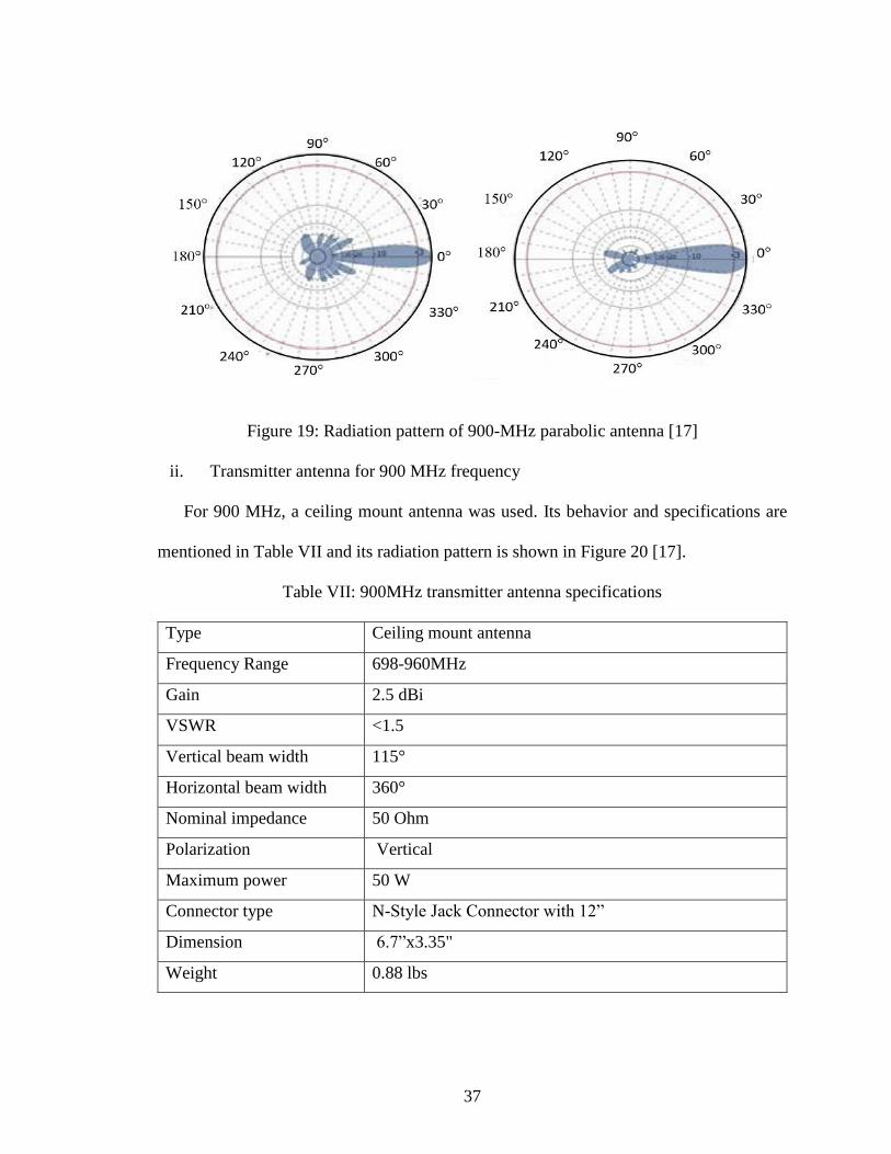
Figure 19: Radiation pattern of 900-MHz parabolic antenna [17]

ii. Transmitter antenna for 900 MHz frequency

For 900 MHz, a ceiling mount antenna was used. Its behavior and specifications are

mentioned in Table VII and its radiation pattern is shown in Figure 20 [17].

Table VII: 900MHz transmitter antenna specifications

Type Ceiling mount antenna

Frequency Range 698-960MHz

Gain 2.5 dBi

VSWR <1.5

Vertical beam width 115°

Horizontal beam width 360°

Nominal impedance 50 Ohm

Polarization Vertical

Maximum power 50 W

Connector type N-Style Jack Connector with 12”

Dimension 6.7”x3.35"

Weight 0.88 lbs

38

Figure 20: Radiation pattern of 900MHz ceiling mount antenna [17]

4.6. Channel Model

The properties of signal propagation in soil need a standard derivation of the path loss

considering all the properties of soil like humidity, texture, and dielectric [6]. From the

Friis equation, which was derived for a free space the received signal power is

𝑃𝑟 = 𝑃𝑡 + 𝐺𝑟 + 𝐺𝑡 − 𝐿0 (1)

where 𝑃𝑡 is the transmit power, 𝐺𝑟 is gains of the receiver and 𝐺𝑡 gain of transmitter

transmitter antennas, 𝐿0 is the path loss,

𝐿0 = 32.4 + 20𝑙𝑜𝑔(𝑑) + 20𝑙𝑜𝑔(𝑓) (2)

where d is the distance between stations, f is operating frequency.

The power of received signal in soil is expressed as

𝑃𝑟 = 𝑃𝑡 + 𝐺𝑟 + 𝐺𝑡 − 𝐿𝑝 (3)

𝐿𝑝 = 𝐿0 + 𝐿𝑠, 𝐿𝑠 is the path loss due to the underground environment. The path loss, 𝐿𝑠 is

based on two factors

39

𝐿𝑠 = 𝐿𝛽 + 𝐿𝛼 (4)

𝐿𝛽 is the attenuation because of difference of the . 𝜆 of the signal in soil environment

𝐿𝛽 = 154 − 20𝑙𝑜𝑔(𝑓) + 20𝑙𝑜𝑔(𝛽), 𝐿𝛼 = 8.69𝛼𝑑 (5)

The path loss in free space is 𝐿0 = 20𝑙𝑜𝑔(4𝜋𝑑/𝜆0))and the path loss 𝐿𝑝, of an EM wave

in soil is as given as:

𝐿𝑝 = 6.4 + 20𝑙𝑜𝑔(𝑑) + 20𝑙𝑜𝑔(𝛽) + 8.69𝛼𝑑 (6)

Where d is the distance, α is the attenuation constant and β phase shifting

Using Peplinski’s principle [20], the dielectric properties of soil for a range of 0.3–1.3 GHz

is given by :

𝜖 = 𝜖′ − 𝑗𝜖″ (7)

𝜖′ = 1.15[1 +𝜌𝑏

𝜌𝑠(𝜖𝑠

𝛼′) + 𝑚𝑣

𝛽′

𝜖𝑓𝑤

′𝛼′− 𝑚𝑣]1 𝛼′⁄ − 0.68 (8)

𝜖″ = [𝑚𝑣𝛽″

𝜖𝑓𝑤

″𝛼′]1 𝛼′⁄ (9)

where 𝜖 is the relative complex dielectric constant of the soil–water mixture, 𝑚𝑣 is the

water volume fraction, 𝜌𝑏 is the bulk density, 𝜌𝑠 = 2.66𝑔/cm3 is the specific density of

the solid soil particles

𝛼′ = 0.65 is an empirically determined constant

𝛽′and 𝛽″are empirically determined constants, and is given by

𝛽′ = 1.2748 − 0.519𝑆 − 0.152𝐶 (10)

𝛽″ = 1.33797 − 0.603𝑆 − 0.166𝐶 (11)

where 𝑆 is the mass fractions of sand and 𝐶 is the mass fractions of clay.. The 𝜖𝑓𝑤

′

and 𝜖𝑓𝑤

″ are the real part and imaginary part of the dielectric constant of water. The

40

propagation constant of the Electromagnet(EM) wave in soil is given by 𝛾 = 𝛼 + 𝑗𝛽

where,

𝛼 = 𝜔√𝜇𝜖′

2[√1 + (

𝜖″

𝜖′)2 − 1]

(12)

𝛽 = 𝜔√𝜇𝜖′

2[√1 + (

𝜖″

𝜖′)2 + 1]

(13)

Figure 21: Path loss with respect to distance

It can be seen that the path loss increases with increasing distance 𝑑, as expected.

Moreover, increasing operating frequency 𝑓, also increases path loss, which motivates the

need for lower frequencies for underground communication. From the Figure 21 [6], we

can conclude that communication is possible at frequency range of 450 to 900 MHz up to

three meters depth, as the path loss is less than 90dB and the receiver sensitivity is -90dB.

So we can conclude that the transmission is possible up to 3 meters without adding extra

power to the transmitter antenna.

41

4.7. Demodulation Scheme

The QPSK receiver employs threshold detectors that detect imaginary and real parts.

The block diagram of the QPSK receiver is shown in Figure 22.

Figure 22: QPSK demodulator

In the demodulator, the received signal is multiplied by a reference frequency sin(ωt)

and cos(ωt). The multiplied output at each arm is then integrated. A threshold detector

decides on each integrated bit which is based on the threshold. Lastly, the bits on the

quadrature arm (i.e odd bits) and the in-phase arm (i.e even bits) are remapped to form the

detected information stream.

4.8. Data Display using HTML

A local python server is created in the surface subsystem, which in turn displays the

received data in Hypertext Markup Language (HTML). A screenshot of sensor data

displayed in HTML is shown in Figure 23. The values in the table are raw data from the

42

Analog to Digital Converter with time stamp, it can be calibrated according to application

and supply voltage to convert it into International System of units (SI Units). You can

observe that the data are logged every second. The sensor values are displayed in degree

Celsius, the humidity and moisture sensor are displayed as raw data. Other channels were

not connected to any sensors.

Figure 23: HTML display of sensor data

43

5. EXPERIMENT RESULTS

5.1. Sensor Data

Sensor data read by the MPC 3008 is transfered to the Raspberry pi through SPI

communication. A screenshot of data acquisition at the Raspberry Pi using a final python

script is shown in Figure 24. You can observe that all 8 channel raw data are displayed, it

was calibrated to view in SI unit on a HTML page.

Figure 24: Raw sensor data read by a terminal python program.

The raw data is compared with threshold values within the Python script to check

for any warnings or possibilities of water leakage, but this is just for observation and not

the final decision. The Python program then saves the raw sensor data into a .csv file along

with the time stamp. Figure 25 is a screenshot of .csv file generated with a sampling rate

of 1 second, sampling period can be varied as per requirements with a maximum sampling

rate of 200K samples per second. Temperature is displayed in degree Celsius, humidity

44

and moisture values are raw data, and this can be calibrated based on application specific

environment.

Figure 25: Raw sensor data saved in .csv format

5.2. GNU Radio Program

The .csv file generated by the python script is then processed in GNU Radio. The block

generated by GNU radio python script where the .csv file is encoded and then QPSK

modulated is shown in Figure 26. The flow graphs are coded in C++ programming

language where python links the blocks together as shown in Figure 26. In the flowgraph

the .csv file generated by the python script is encoded using 2 bits/symbol and 4 samples/

symbol. The encoded signal is then QPSK modulated and transmitted to HackRF one

module using Open Source Mobile Communication (OSMOCOM) sink at 450 MHz and

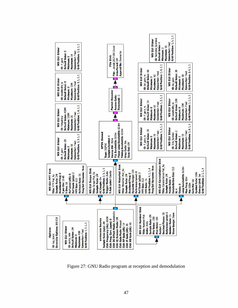
900 MHz operating frequency. The GNU Radio receiver top block is shown in Figure 27.

The received signal from the high gain antenna is fed to HackRF one module then

transferred to a computer through a USB. The received data from HAckRF One is

processed in GNU Radio where the signal is demodulated and decoded to generate a .csv

45

file. A GNU Radio program was developed to encode and modulate signal with an option

of varying parameters like Operating frequency, sampling frequency, Receiver/transmitter

gain, modulation schemes, amplitude, samples per symbol, bits per symbol etc,.

46

Figure 26: GNU Radio program for modulation and transmission

47

Figure 27: GNU Radio program at reception and demodulation

48

5.3. Transmitted and Received Signal Analysis

The spectrum of the transmitted signal at given frequency can be viewed using Fast

Fourier Transforms (FFT) plot of GNU Radio Figure 28. It can observed in FFT plot that

the signal components are transmitted from 449.6MHz to 450.4MHz .The average signal

power of transmitted signal is about -25dB. The bandwidth of the system is 800 KHz with

a center frequency of 450MHz. The spectrum analyzer was used to capture received signal

and is shown in Figure 29 with a bandwidth of 800 KHz and signal power about -45dB.

Figure 28: FFT plot of transmitted signal at 450MHz

49

Figure 29: Spectrum analyser output of received signal at 450MHz

The QPSK modulated signal fits in four quadrants of the constellation as seen in

Figure 30. As explained in the previous chapter, the message signals are represented in four

quadrants. In this experiment, 2 bits/symbols are used which in turn represents 4

samples/symbol. The modulated signal is then transmitted using an OSMOCOM sink,

which programs Hack RF SDR to send the modulated signal with the specified parameters.

A perfect constellation that are in phase with the transmitted signal with only few out of

phase was received at the surface subsystem that can be seen in, which is then demodulated

to regenerate the data that was transmitted.

50

Figure 30: Constellation plot of transmitted signal at 450 MHz

Figure 31: Constellation plot of received signal at 450 MHz

The waterfall diagram of the transmitted signal at 450 MHz and 900MHz are shown

in Figure 32 and Figure 34, which has a bandwidth of 800 KHz. It can be seen that

frequency outside the bandwidth has relatively low power (below -100dB). It can be

observed that the transmitted signal has power of -25dB there by decreasing the power

consumption of transmitter that is buried underground. The waterfall diagram of the

51

received signal at 450MHz and 900 MHz are shown in Figure 33 and Figure 35. It can be

observed in received signals noises are of low power compared to the required message

signal.

Figure 32: Waterfall diagram of transmitted signal at 450MHz

Figure 33: Waterfall diagram of received signal at 450MHz

52

Figure 34: Waterfall diagram of transmitted signal at 900MHz

Figure 35: Waterfall diagram of received signal at 900MHz

The constellation diagram is for understanding the modulated signal. However, the

signal transmitted in real time is shown in Figure 36 , any change in phase represents

change in digital data. A 1 volt amplitude with quadrature phase shift modulated signal is

transmitted at 900MHz over an OSMOCOM source. The received signal is captured in

GNU radio and spectrum analyzer as shown in Figure 37 and Figure 38.

53

Figure 36: Signal scope of transmitted signal a 900 MHz

Figure 37: Signal scope of received signal at 900 MHz

54

Figure 38: Signal scope of received signal

A dummy file was transmitted continuously with known sequence with specified

frequency, bandwidth, and transmission gain. The modulation schemes used in analysis are

PSK, QPSK and 8-PSK with different burial depths. The main measurements that decide

the performance of communication systems like Signal to Noise Ratio(SNR), data rate was

calculated. The SNR was calculated by using Signal to Noise ratio estimator probe in GNU

Radio. It can be observed from Table VIII, that SNR decreases as the burrial depth

increases. SNR plays an important role in communication, as signal power should be

stronger than the noise power. The flow of experiment is as shown in Figure 39. To

calculate all the important parameters of communication like SNR, and Data rate, a dummy

file of known sequence was sent for a duration of 10 seconds from subsurface transmitter

and received at surface receiver and then checking the size of the received file. The

experiment was carried out at two frequencies 450 MHZ and 900 MHZ keeping the

bandwidth constant at 800MHz.The burial depth was varied from 0.5 meters to 1.5 meters

to understand the effect of burial distance as shown in Figure 39. All the experiment was

carried out for 5 iterations and an average of all are mentioned in Table 6. It can be observed

that the data rate increased as the modulation scheme was changed from PSK to QPSK and

55

It increased more when the modulation scheme was changed from QPSK to 8 PSK.

However, 8 PSK will have more error rate compared to QPSK. Comparing all the

parameters in Table VIII. QPSK at a operating frequency of 900 MHz was best suited for

WUSN as it yields a good data rate of 1.253 Mbps and SNR of 24.265. for the given

underground environment.

Dummy File of Known Sequence

(Send for 10 Seconds)Packet Encoder

Modulate• PSK• QPSK• 8 PSK

TransmitterHackRF

Underground Environment • Varied depth from 0.5, 1, 1.5 Meters• 2.Bandwidth 800KHz• Operating Frequency 450MHz/

900MHz

ReceiverHackRF

Demodulate• PSK• QPSK• 8 PSK

Packet DecoderDummy File of Known

Sequence(Receive for 10 Seconds)

GNU Radio

SNR Estimator ProbeSignal to Noise Ratio

Figure 39: Experimental testbed for calculating data rate and SNR

56

Table VIII: Data transmission analysis

Mod

scheme

Tx

gain

Rx

gain

C.freq BW Depth

dist in

meters

Avg

SNR

Avg

Tx

time

in

sec

Avg

data

received

in 10 sec

Avg

data

rate per

sec

BPSK 0 dB 30 dB 450MHz 0.8MHz 1.5 24.534 10

6.45

Mbits

0.645

Mbps

QPSK 0 dB 30 dB 450MHz 0.8MHz 1.5 24.265 10

12.53

Mbits

1.253

Mbps

8 PSK 0 dB 30 dB 450MHz 0.8MHz 1.5 24.452 10

21.95

Mbits

2.195

Mbps

BPSK 0 dB 30 dB 900MHz 0.8MHz 1.5 24.534 10

12.45

Mbits

1.245

Mbps

QPSK 0 dB 30 dB 900MHz 0.8MHz 1.5 24.265 10

19.53

Mbits

1.953

Mbps

8 PSK 0 dB 30 dB 900MHz 0.8MHz 1.5 24.452 10

28.95

Mbits

2.895

Mbps

BPSK 0 dB 30 dB 450MHz 0.8MHz 1 26.776 10

6.59

Mbits

0.659

Mbps

QPSK 0 dB 30 dB 450MHz 0.8MHz 1 26.522 10

11.96

Mbits

1.196

Mbps

8 PSK 0 dB 30 dB 450MHz 0.8MHz 1 26.254 10

19.94

Mbits

1.994

Mbps

BPSK 0 dB 30 dB 900MHz 0.8MHz 1 26.244 10

13.35

Mbits

1.335

Mbps

QPSK 0 dB 30 dB 900MHz 0.8MHz 1 26.244 10

19.86

Mbits

1.986

Mbps

8 PSK 0 dB 30 dB 900MHz 0.8MHz 1 26.344 10

29.56

Mbits

2.956

Mbps

BPSK 0 dB 30 dB 450MHz 0.8MHz 0.5 27.853 10

9.33

Mbits

0.933

Mbps

QPSK 0 dB 30 dB 450MHz 0.8MHz 0.5 27.742 10

10.96

Mbits

1.096

Mbps

8 PSK 0 dB 30 dB 450MHz 0.8MHz 0.5 27.722 10

29.96

Mbits

2.996

Mbps

BPSK 0 dB 30 dB 900MHz 0.8MHz 0.5 27.692 10

13.86

Mbits

1.386

Mbps

QPSK 0 dB 30 dB 900MHz 0.8MHz 0.5 28.124 10

25.01

Mbits

2.501

Mbps

8 PSK 0 dB 30 dB 900MHz 0.8MHz 0.5 27.985 10

31.45

Mbits

3.145

Mbps

Note :

Mod Scheme – Modulation scheme

Tx gain – Transmitter gain

57

Rx – Receiver gain

C. freq –Center frequency

BW – Bandwidth

Depth dist in meters – Depth distance in meters

Avg SNR – Average Signal to Noise Ratio (SNR)

Avg Tx time in sec – Average Transmission time in seconds

Avg data received in 10 sec – Average dara rate in 10 seconds

Avg data rate per sec – Average data rate per second

Mbits – Mega bits

Mbps – Mega bits per second

58

5.4. HTML display

The .csv file generated by GNU Radio is then displayed in an HTML page as shown

in Figure 40. A local python server was used to display the csv file generated by GNU

Radio is then displayed in an HTML page as shown in Figure 40.

Figure 40: Displaying the received data in HTML page

59

6. CONCLUSION

A study about the impact of operating frequency, modulation scheme, and signal power

with respect to burial depth, soil characteristics, and antenna design of buried underground

wireless sensor network is investigated. Characterization of wireless sensor network for

detection of water leakage in underground pipes was carried out. The subsurface subsystem

was buried, and the system was able to communicate with the surface subsystem. The

surface subsystem was able to log and process the sensor data. An innovative test-bed was

designed and built to test the capability of the system to establish communication and

transmit the sensor data under lossy environment. The measured data was transmitted

wirelessly to the surface system on a real-time basis for monitoring and further analysis.

The system was capable of working under a subsurface environments and communicate

with the surface module at a frequency range of 450MHz to 900MHz. The results show

WUSN’s ability to communicate successfully and detect water leakages in the pipeline

which was be buried 2 meters from the earth’s surface.

Future work of the research is to replace the Software Defined Radio with a

conventional hardware radio. By doing this a lot of power can be saved which can be used

to operate the subsurface system for a longer duration. Generating power by installing

transducers that can use underground sources like temperature, vibration, flow, etc. can

increase the life of the subsurface subsystem and could be implemented. An alternative to

electromagnetic (EM) propagation can be used like Magnetic-Induction (MI) to increase

the operating frequency.

60

APPENDIX

APPENDIX A

GNU Radio QPSK transmitter code – top_block.py

#!/usr/bin/env python2

# -*- coding: utf-8 -*-

##################################################

# GNU Radio Python Flow Graph

# Title: Top Block

# Generated: Wed Oct 18 17:49:55 2017

##################################################

if __name__ == '__main__':

import ctypes

import sys

if sys.platform.startswith('linux'):

try:

x11 = ctypes.cdll.LoadLibrary('libX11.so')

x11.XInitThreads()

except:

print "Warning: failed to XInitThreads()"

from gnuradio import blocks

from gnuradio import digital

from gnuradio import eng_notation

from gnuradio import gr

from gnuradio import wxgui

from gnuradio.eng_option import eng_option

from gnuradio.fft import window

from gnuradio.filter import firdes

from gnuradio.wxgui import constsink_gl

from gnuradio.wxgui import fftsink2

from gnuradio.wxgui import forms

from gnuradio.wxgui import scopesink2

from grc_gnuradio import blks2 as grc_blks2

61

from grc_gnuradio import wxgui as grc_wxgui

from optparse import OptionParser

import osmosdr

import time

import wx

class top_block(grc_wxgui.top_block_gui):

def __init__(self):

grc_wxgui.top_block_gui.__init__(self, title="Top Block")

_icon_path =

"/usr/share/icons/hicolor/32x32/apps/gnuradio-grc.png"

self.SetIcon(wx.Icon(_icon_path, wx.BITMAP_TYPE_ANY))

##################################################

# Variables

##################################################

self.samp_rate = samp_rate = 2e6

self.rf_gain_rx = rf_gain_rx = 14

self.no_constellation = no_constellation = 4

self.lowFerq = lowFerq = 140e6

self.if_gain_rx = if_gain_rx = 40

self.bb_gain_rx = bb_gain_rx = 40

self.bandwidth_rx = bandwidth_rx = 10e6

self.Frequency = Frequency = 450e6

##################################################

# Blocks

##################################################

_samp_rate_sizer = wx.BoxSizer(wx.VERTICAL)

self._samp_rate_text_box = forms.text_box(

parent=self.GetWin(),

sizer=_samp_rate_sizer,

value=self.samp_rate,

callback=self.set_samp_rate,

label='samp_rate',

converter=forms.float_converter(),

proportion=0,

62

)

self._samp_rate_slider = forms.slider(





minimum=0,

maximum=40e6,

num_steps=100,

style=wx.SL_VERTICAL,

cast=float,

proportion=1,

)

self.GridAdd(_samp_rate_sizer, 1, 3, 1, 1)

_rf_gain_rx_sizer = wx.BoxSizer(wx.VERTICAL)

self._rf_gain_rx_text_box = forms.text_box(


sizer=_rf_gain_rx_sizer,

value=self.rf_gain_rx,

callback=self.set_rf_gain_rx,

label='rf_gain_rx',


proportion=0,

)

self._rf_gain_rx_slider = forms.slider(





minimum=0,

maximum=50,

num_steps=51,


cast=float,

63

proportion=1,

)

self.GridAdd(_rf_gain_rx_sizer, 1, 8, 1, 1)

_no_constellation_sizer = wx.BoxSizer(wx.VERTICAL)

self._no_constellation_text_box = forms.text_box(


sizer=_no_constellation_sizer,

value=self.no_constellation,

callback=self.set_no_constellation,

label='no_constellation',


proportion=0,

)

self._no_constellation_slider = forms.slider(


sizer=_no_constellation_sizer,

value=self.no_constellation,

callback=self.set_no_constellation,

minimum=2,

maximum=12,

num_steps=12,


cast=float,

proportion=1,

)

self.GridAdd(_no_constellation_sizer, 1, 2, 1, 1)

_if_gain_rx_sizer = wx.BoxSizer(wx.VERTICAL)

self._if_gain_rx_text_box = forms.text_box(


sizer=_if_gain_rx_sizer,

value=self.if_gain_rx,

callback=self.set_if_gain_rx,

label='if_gain_rx',


64

proportion=0,

)

self._if_gain_rx_slider = forms.slider(





minimum=0,

maximum=40,

num_steps=5,


cast=float,

proportion=1,

)

self.GridAdd(_if_gain_rx_sizer, 1, 5, 1, 1)

_bb_gain_rx_sizer = wx.BoxSizer(wx.VERTICAL)

self._bb_gain_rx_text_box = forms.text_box(


sizer=_bb_gain_rx_sizer,

value=self.bb_gain_rx,

callback=self.set_bb_gain_rx,

label='bb_gain_rx',


proportion=0,

)

self._bb_gain_rx_slider = forms.slider(





minimum=0,

maximum=62,

num_steps=31,


65

cast=float,

proportion=1,

)

self.GridAdd(_bb_gain_rx_sizer, 1, 6, 1, 1)

_bandwidth_rx_sizer = wx.BoxSizer(wx.VERTICAL)

self._bandwidth_rx_text_box = forms.text_box(


sizer=_bandwidth_rx_sizer,

value=self.bandwidth_rx,

callback=self.set_bandwidth_rx,

label='bandwidth_rx',


proportion=0,

)

self._bandwidth_rx_slider = forms.slider(





minimum=0,

maximum=10e6,

num_steps=1000,

style=wx.SL_HORIZONTAL,

cast=float,

proportion=1,

)

self.GridAdd(_bandwidth_rx_sizer, 1, 7, 1, 1)

_Frequency_sizer = wx.BoxSizer(wx.VERTICAL)

self._Frequency_text_box = forms.text_box(


sizer=_Frequency_sizer,

value=self.Frequency,

callback=self.set_Frequency,

label='Frequency',

66


proportion=0,

)

self._Frequency_slider = forms.slider(





minimum=100e6,

maximum=2e9,

num_steps=1000,


cast=float,

proportion=1,

)

self.GridAdd(_Frequency_sizer, 1, 4, 1, 1)

self.wxgui_scopesink2_0 = scopesink2.scope_sink_c(

self.GetWin(),

title="Scope Plot",

sample_rate=samp_rate,

v_scale=0,

v_offset=0,

t_scale=0,

ac_couple=False,

xy_mode=False,

num_inputs=1,

trig_mode=wxgui.TRIG_MODE_AUTO,

y_axis_label="Counts",

)

self.Add(self.wxgui_scopesink2_0.win)

self.wxgui_fftsink2_0 = fftsink2.fft_sink_c(

self.GetWin(),

baseband_freq=0,

y_per_div=10,

67

y_divs=10,

ref_level=0,

ref_scale=2.0,


fft_size=1024,

fft_rate=15,

average=False,

avg_alpha=None,

title="FFT Plot",

peak_hold=False,

win=window.blackmanharris,

)

self.Add(self.wxgui_fftsink2_0.win)

self.wxgui_constellationsink2_0_0 =

constsink_gl.const_sink_c(

self.GetWin(),

title="Constellation Plot_rx",


frame_rate=5,

const_size=2048/4,

M=4,

theta=0,

loop_bw=6.28/100.0,

fmax=0.06,

mu=0.5,

gain_mu=0.005,

symbol_rate=samp_rate/4.,

omega_limit=0.005,

)

self.GridAdd(self.wxgui_constellationsink2_0_0.win, 2, 1,

1, 5)

self.osmosdr_source_0 = osmosdr.source( args="numchan=" +

str(1) + " " + "" )

self.osmosdr_source_0.set_sample_rate(samp_rate)

68

self.osmosdr_source_0.set_center_freq(Frequency, 0)

self.osmosdr_source_0.set_freq_corr(0, 0)

self.osmosdr_source_0.set_dc_offset_mode(0, 0)

self.osmosdr_source_0.set_iq_balance_mode(0, 0)

self.osmosdr_source_0.set_gain_mode(False, 0)

self.osmosdr_source_0.set_gain(rf_gain_rx, 0)

self.osmosdr_source_0.set_if_gain(if_gain_rx, 0)

self.osmosdr_source_0.set_bb_gain(bb_gain_rx, 0)

self.osmosdr_source_0.set_antenna("", 0)

self.osmosdr_source_0.set_bandwidth(bandwidth_rx, 0)

_lowFerq_sizer = wx.BoxSizer(wx.VERTICAL)

self._lowFerq_text_box = forms.text_box(


sizer=_lowFerq_sizer,

value=self.lowFerq,

callback=self.set_lowFerq,

label='lowFerq',


proportion=0,

)

self._lowFerq_slider = forms.slider(


sizer=_lowFerq_sizer,

value=self.lowFerq,

callback=self.set_lowFerq,

minimum=0,

maximum=1e9,

num_steps=1000,


cast=float,

proportion=1,

)

self.GridAdd(_lowFerq_sizer, 1, 1, 1, 1)

self.digital_psk_demod_0 = digital.psk.psk_demod(

69

constellation_points=no_constellation,

differential=True,

samples_per_symbol=4,

excess_bw=0.35,

phase_bw=6.28/100.0,

timing_bw=6.28/100.0,

mod_code="gray",

verbose=False,

log=False,

)

self.blocks_file_sink_0 =

blocks.file_sink(gr.sizeof_char*1,

"/home/raghu/Desktop/Server_Sensor/received_0926.csv", False)

self.blocks_file_sink_0.set_unbuffered(True)

self.blks2_packet_decoder_0 =

grc_blks2.packet_demod_b(grc_blks2.packet_decoder(

access_code="",

threshold=-1,

callback=lambda ok, payload:

self.blks2_packet_decoder_0.recv_pkt(ok, payload),

),

)

##################################################

# Connections

##################################################

self.connect((self.blks2_packet_decoder_0, 0),

(self.blocks_file_sink_0, 0))

self.connect((self.digital_psk_demod_0, 0),

(self.blks2_packet_decoder_0, 0))

self.connect((self.osmosdr_source_0, 0),

(self.digital_psk_demod_0, 0))


(self.wxgui_constellationsink2_0_0, 0))

70


(self.wxgui_fftsink2_0, 0))


(self.wxgui_scopesink2_0, 0))

def get_samp_rate(self):

return self.samp_rate

def set_samp_rate(self, samp_rate):

self.samp_rate = samp_rate

self._samp_rate_slider.set_value(self.samp_rate)

self._samp_rate_text_box.set_value(self.samp_rate)

self.osmosdr_source_0.set_sample_rate(self.samp_rate)

self.wxgui_constellationsink2_0_0.set_sample_rate(self.samp_rate)

self.wxgui_fftsink2_0.set_sample_rate(self.samp_rate)

self.wxgui_scopesink2_0.set_sample_rate(self.samp_rate)

def get_rf_gain_rx(self):

return self.rf_gain_rx

def set_rf_gain_rx(self, rf_gain_rx):

self.rf_gain_rx = rf_gain_rx

self._rf_gain_rx_slider.set_value(self.rf_gain_rx)

self._rf_gain_rx_text_box.set_value(self.rf_gain_rx)

self.osmosdr_source_0.set_gain(self.rf_gain_rx, 0)

def get_no_constellation(self):

return self.no_constellation

def set_no_constellation(self, no_constellation):

self.no_constellation = no_constellation

self._no_constellation_slider.set_value(self.no_constellation)

self._no_constellation_text_box.set_value(self.no_constellation)

def get_lowFerq(self):

return self.lowFerq

def set_lowFerq(self, lowFerq):

self.lowFerq = lowFerq

71

self._lowFerq_slider.set_value(self.lowFerq)

self._lowFerq_text_box.set_value(self.lowFerq)

def get_if_gain_rx(self):

return self.if_gain_rx

def set_if_gain_rx(self, if_gain_rx):

self.if_gain_rx = if_gain_rx

self._if_gain_rx_slider.set_value(self.if_gain_rx)

self._if_gain_rx_text_box.set_value(self.if_gain_rx)

self.osmosdr_source_0.set_if_gain(self.if_gain_rx, 0)

def get_bb_gain_rx(self):

return self.bb_gain_rx

def set_bb_gain_rx(self, bb_gain_rx):

self.bb_gain_rx = bb_gain_rx

self._bb_gain_rx_slider.set_value(self.bb_gain_rx)

self._bb_gain_rx_text_box.set_value(self.bb_gain_rx)

self.osmosdr_source_0.set_bb_gain(self.bb_gain_rx, 0)

def get_bandwidth_rx(self):

return self.bandwidth_rx

def set_bandwidth_rx(self, bandwidth_rx):

self.bandwidth_rx = bandwidth_rx

self._bandwidth_rx_slider.set_value(self.bandwidth_rx)

self._bandwidth_rx_text_box.set_value(self.bandwidth_rx)

self.osmosdr_source_0.set_bandwidth(self.bandwidth_rx, 0)

def get_Frequency(self):

return self.Frequency

def set_Frequency(self, Frequency):

self.Frequency = Frequency

self._Frequency_slider.set_value(self.Frequency)

self._Frequency_text_box.set_value(self.Frequency)

self.osmosdr_source_0.set_center_freq(self.Frequency, 0)

def main(top_block_cls=top_block, options=None):

tb = top_block_cls()

tb.Start(True)

tb.Wait()

72

if __name__ == '__main__':

main()

73

APPENDIX B

GNU Radio QPSK receiver code – top_block.py

#!/usr/bin/env python2

# -*- coding: utf-8 -*-

##################################################

# GNU Radio Python Flow Graph

# Title: Top Block

# Generated: Sun Oct 22 00:34:55 2017

##################################################

if __name__ == '__main__':

import ctypes

import sys

if sys.platform.startswith('linux'):

try:

x11 = ctypes.cdll.LoadLibrary('libX11.so')

x11.XInitThreads()

except:

print "Warning: failed to XInitThreads()"

from gnuradio import blocks

from gnuradio import digital

from gnuradio import eng_notation

from gnuradio import gr

from gnuradio import wxgui

from gnuradio.eng_option import eng_option

from gnuradio.fft import window

from gnuradio.filter import firdes

from gnuradio.wxgui import constsink_gl

from gnuradio.wxgui import fftsink2

from gnuradio.wxgui import forms

from gnuradio.wxgui import numbersink2

from gnuradio.wxgui import scopesink2

74

from gnuradio.wxgui import waterfallsink2

from grc_gnuradio import blks2 as grc_blks2

from grc_gnuradio import wxgui as grc_wxgui

from optparse import OptionParser

import osmosdr

import time

import wx

class top_block(grc_wxgui.top_block_gui):

def __init__(self):

grc_wxgui.top_block_gui.__init__(self, title="Top Block")

_icon_path =

"/usr/share/icons/hicolor/32x32/apps/gnuradio-grc.png"

self.SetIcon(wx.Icon(_icon_path, wx.BITMAP_TYPE_ANY))

##################################################

# Variables

##################################################

self.samp_rate = samp_rate = 2e6

self.rf_gain_rx = rf_gain_rx = 14

self.rf_gain = rf_gain = 0

self.if_gain_rx = if_gain_rx = 30

self.if_gain = if_gain = 20

self.bb_gain_rx = bb_gain_rx = 45

self.bb_gain = bb_gain = 30

self.bandwidth_tx = bandwidth_tx = 0

self.bandwidth_rx = bandwidth_rx = 10e6

self.Samples_Symbols = Samples_Symbols = 4

self.Frequency = Frequency = 450e6

self.Bits_Symbol = Bits_Symbol = 2

##################################################

75

# Blocks

##################################################

_samp_rate_sizer = wx.BoxSizer(wx.VERTICAL)

self._samp_rate_text_box = forms.text_box(





label='samp_rate',


proportion=0,

)

self._samp_rate_slider = forms.slider(





minimum=0,

maximum=40e6,

num_steps=100,


cast=float,

proportion=1,

)

self.GridAdd(_samp_rate_sizer, 1, 7, 1, 1)

_rf_gain_rx_sizer = wx.BoxSizer(wx.VERTICAL)

self._rf_gain_rx_text_box = forms.text_box(





label='rf_gain_rx',


proportion=0,

76

)

self._rf_gain_rx_slider = forms.slider(





minimum=0,

maximum=50,

num_steps=51,


cast=float,

proportion=1,

)

self.GridAdd(_rf_gain_rx_sizer, 1, 2, 1, 1)

_if_gain_rx_sizer = wx.BoxSizer(wx.VERTICAL)

self._if_gain_rx_text_box = forms.text_box(





label='if_gain_rx',


proportion=0,

)

self._if_gain_rx_slider = forms.slider(





minimum=0,

maximum=70,

num_steps=5,


cast=float,

77

proportion=1,

)

self.GridAdd(_if_gain_rx_sizer, 1, 3, 1, 1)

_bb_gain_rx_sizer = wx.BoxSizer(wx.VERTICAL)

self._bb_gain_rx_text_box = forms.text_box(





label='bb_gain_rx',


proportion=0,

)

self._bb_gain_rx_slider = forms.slider(





minimum=0,

maximum=62,

num_steps=31,


cast=float,

proportion=1,

)

self.GridAdd(_bb_gain_rx_sizer, 1, 4, 1, 1)

_Samples_Symbols_sizer = wx.BoxSizer(wx.VERTICAL)

self._Samples_Symbols_text_box = forms.text_box(


sizer=_Samples_Symbols_sizer,

value=self.Samples_Symbols,

callback=self.set_Samples_Symbols,

label='Samples_Symbols',


78

proportion=0,

)

self._Samples_Symbols_slider = forms.slider(


sizer=_Samples_Symbols_sizer,

value=self.Samples_Symbols,

callback=self.set_Samples_Symbols,

minimum=2,

maximum=16,

num_steps=12,


cast=float,

proportion=1,

)

self.GridAdd(_Samples_Symbols_sizer, 1, 5, 1, 1)

_Frequency_sizer = wx.BoxSizer(wx.VERTICAL)

self._Frequency_text_box = forms.text_box(





label='Frequency',


proportion=0,

)

self._Frequency_slider = forms.slider(





minimum=100e6,

maximum=2e9,

num_steps=1000,


79

cast=float,

proportion=1,

)

self.GridAdd(_Frequency_sizer, 1, 6, 1, 1)

self.wxgui_waterfallsink_Tx =

waterfallsink2.waterfall_sink_c(

self.GetWin(),

baseband_freq=Frequency,

dynamic_range=100,

ref_level=0,

ref_scale=2.0,


fft_size=512,

fft_rate=15,

average=False,

avg_alpha=None,

title="Waterfall Plot_Rx",

)

self.GridAdd(self.wxgui_waterfallsink_Tx.win, 2, 1, 1, 4)

self.wxgui_scopesink2_0 = scopesink2.scope_sink_c(

self.GetWin(),

title="Scope Plot_Rx",


v_scale=0,

v_offset=0,

t_scale=0,

ac_couple=True,

xy_mode=False,

num_inputs=1,

trig_mode=wxgui.TRIG_MODE_AUTO,

y_axis_label="Counts",

)

self.GridAdd(self.wxgui_scopesink2_0.win, 4, 1, 1, 4)

self.wxgui_numbersink2_1 = numbersink2.number_sink_c(

80

self.GetWin(),

unit="Units",

minval=-100,

maxval=100,

factor=1.0,

decimal_places=10,

ref_level=0,


number_rate=15,

average=False,

avg_alpha=None,

label="Number Plot",

peak_hold=False,

show_gauge=True,

)

self.Add(self.wxgui_numbersink2_1.win)

self.wxgui_fftsink2_0_0 = fftsink2.fft_sink_c(

self.GetWin(),

baseband_freq=Frequency,

y_per_div=10,

y_divs=10,

ref_level=0,

ref_scale=2.0,


fft_size=512,

fft_rate=15,

average=False,

avg_alpha=None,

title="FFT Plot_Rx",

peak_hold=False,

)

self.GridAdd(self.wxgui_fftsink2_0_0.win, 4, 5, 1, 3)

self.wxgui_constellationsink2_0 =

constsink_gl.const_sink_c(

81

self.GetWin(),

title="Constellation Plot_Rx",


frame_rate=5,

const_size=2048/4,

M=4,

theta=0,

loop_bw=6.28/100.0,

fmax=0.06,

mu=0.5,

gain_mu=0.005,

symbol_rate=samp_rate/4.,

omega_limit=0.005,

)

self.GridAdd(self.wxgui_constellationsink2_0.win, 2, 5,

1, 4)

_rf_gain_sizer = wx.BoxSizer(wx.VERTICAL)

self._rf_gain_text_box = forms.text_box(


sizer=_rf_gain_sizer,

value=self.rf_gain,

callback=self.set_rf_gain,

label='rf_gain',


proportion=0,

)

self._rf_gain_slider = forms.slider(


sizer=_rf_gain_sizer,

value=self.rf_gain,

callback=self.set_rf_gain,

minimum=0,

maximum=14,

num_steps=1,

82


cast=float,

proportion=1,

)

self.GridAdd(_rf_gain_sizer, 3, 2, 1, 1)

self.osmosdr_source_2 = osmosdr.source( args="numchan=" +

str(1) + " " + "" )

self.osmosdr_source_2.set_sample_rate(samp_rate)

self.osmosdr_source_2.set_center_freq(Frequency, 0)

self.osmosdr_source_2.set_freq_corr(0, 0)

self.osmosdr_source_2.set_dc_offset_mode(2, 0)

self.osmosdr_source_2.set_iq_balance_mode(0, 0)

self.osmosdr_source_2.set_gain_mode(False, 0)

self.osmosdr_source_2.set_gain(rf_gain_rx, 0)

self.osmosdr_source_2.set_if_gain(if_gain_rx, 0)

self.osmosdr_source_2.set_bb_gain(bb_gain_rx, 0)

self.osmosdr_source_2.set_antenna("", 0)

self.osmosdr_source_2.set_bandwidth(0, 0)

_if_gain_sizer = wx.BoxSizer(wx.VERTICAL)

self._if_gain_text_box = forms.text_box(


sizer=_if_gain_sizer,

value=self.if_gain,

callback=self.set_if_gain,

label='if_gain',


proportion=0,

)

self._if_gain_slider = forms.slider(


sizer=_if_gain_sizer,

value=self.if_gain,

callback=self.set_if_gain,

83

minimum=0,

maximum=50,

num_steps=51,


cast=float,

proportion=1,

)

self.GridAdd(_if_gain_sizer, 3, 3, 1, 1)

self.digital_dxpsk_demod_0 = digital.dqpsk_demod(

samples_per_symbol=Samples_Symbols,

excess_bw=0.35,

freq_bw=6.28/100.0,

phase_bw=6.28/100.0,

timing_bw=6.28/100.0,

mod_code="gray",

verbose=False,

log=False

)

self.blocks_file_sink_1 =

blocks.file_sink(gr.sizeof_char*1, "/home/raghu/Desktop/sensor

data/received_2017-10-13.csv", False)

self.blocks_file_sink_1.set_unbuffered(False)

self.blks2_packet_decoder_1 =

grc_blks2.packet_demod_b(grc_blks2.packet_decoder(

access_code="",

threshold=-1,

callback=lambda ok, payload:

self.blks2_packet_decoder_1.recv_pkt(ok, payload),

),

)

_bb_gain_sizer = wx.BoxSizer(wx.VERTICAL)

self._bb_gain_text_box = forms.text_box(


sizer=_bb_gain_sizer,

84

value=self.bb_gain,

callback=self.set_bb_gain,

label='bb_gain',


proportion=0,

)

self._bb_gain_slider = forms.slider(


sizer=_bb_gain_sizer,

value=self.bb_gain,

callback=self.set_bb_gain,

minimum=0,

maximum=50,

num_steps=51,


cast=float,

proportion=1,

)

self.GridAdd(_bb_gain_sizer, 3, 4, 1, 1)

_bandwidth_tx_sizer = wx.BoxSizer(wx.VERTICAL)

self._bandwidth_tx_text_box = forms.text_box(


sizer=_bandwidth_tx_sizer,

value=self.bandwidth_tx,

callback=self.set_bandwidth_tx,

label='bandwidth_tx',


proportion=0,

)

self._bandwidth_tx_slider = forms.slider(


sizer=_bandwidth_tx_sizer,

value=self.bandwidth_tx,

callback=self.set_bandwidth_tx,

85

minimum=0,

maximum=10e6,

num_steps=1000,


cast=float,

proportion=1,

)

self.GridAdd(_bandwidth_tx_sizer, 3, 1, 1, 1)

_bandwidth_rx_sizer = wx.BoxSizer(wx.VERTICAL)

self._bandwidth_rx_text_box = forms.text_box(





label='bandwidth_rx',


proportion=0,

)

self._bandwidth_rx_slider = forms.slider(





minimum=0,

maximum=10e6,

num_steps=1000,


cast=float,

proportion=1,

)

self.GridAdd(_bandwidth_rx_sizer, 1, 1, 1, 1)

_Bits_Symbol_sizer = wx.BoxSizer(wx.VERTICAL)

self._Bits_Symbol_text_box = forms.text_box(


86

sizer=_Bits_Symbol_sizer,

value=self.Bits_Symbol,

callback=self.set_Bits_Symbol,

label='Bits_Symbol',


proportion=0,

)

self._Bits_Symbol_slider = forms.slider(


sizer=_Bits_Symbol_sizer,

value=self.Bits_Symbol,

callback=self.set_Bits_Symbol,

minimum=2,

maximum=16,

num_steps=8,


cast=float,

proportion=1,

)

self.GridAdd(_Bits_Symbol_sizer, 1, 8, 1, 1)

##################################################

# Connections

##################################################

self.connect((self.blks2_packet_decoder_1, 0),

(self.blocks_file_sink_1, 0))

self.connect((self.digital_dxpsk_demod_0, 0),

(self.blks2_packet_decoder_1, 0))


(self.digital_dxpsk_demod_0, 0))


(self.wxgui_constellationsink2_0, 0))


(self.wxgui_fftsink2_0_0, 0))

87


(self.wxgui_numbersink2_1, 0))


(self.wxgui_scopesink2_0, 0))


(self.wxgui_waterfallsink_Tx, 0))

def get_samp_rate(self):

return self.samp_rate

def set_samp_rate(self, samp_rate):

self.samp_rate = samp_rate

self._samp_rate_slider.set_value(self.samp_rate)

self._samp_rate_text_box.set_value(self.samp_rate)

self.osmosdr_source_2.set_sample_rate(self.samp_rate)

self.wxgui_constellationsink2_0.set_sample_rate(self.samp_rate)

self.wxgui_fftsink2_0_0.set_sample_rate(self.samp_rate)

self.wxgui_scopesink2_0.set_sample_rate(self.samp_rate)

self.wxgui_waterfallsink_Tx.set_sample_rate(self.samp_rate)

def get_rf_gain_rx(self):

return self.rf_gain_rx

def set_rf_gain_rx(self, rf_gain_rx):

self.rf_gain_rx = rf_gain_rx

self._rf_gain_rx_slider.set_value(self.rf_gain_rx)

self._rf_gain_rx_text_box.set_value(self.rf_gain_rx)

self.osmosdr_source_2.set_gain(self.rf_gain_rx, 0)

def get_rf_gain(self):

return self.rf_gain

88

def set_rf_gain(self, rf_gain):

self.rf_gain = rf_gain

self._rf_gain_slider.set_value(self.rf_gain)

self._rf_gain_text_box.set_value(self.rf_gain)

def get_if_gain_rx(self):

return self.if_gain_rx

def set_if_gain_rx(self, if_gain_rx):

self.if_gain_rx = if_gain_rx

self._if_gain_rx_slider.set_value(self.if_gain_rx)

self._if_gain_rx_text_box.set_value(self.if_gain_rx)

self.osmosdr_source_2.set_if_gain(self.if_gain_rx, 0)

def get_if_gain(self):

return self.if_gain

def set_if_gain(self, if_gain):

self.if_gain = if_gain

self._if_gain_slider.set_value(self.if_gain)

self._if_gain_text_box.set_value(self.if_gain)

def get_bb_gain_rx(self):

return self.bb_gain_rx

def set_bb_gain_rx(self, bb_gain_rx):

self.bb_gain_rx = bb_gain_rx

self._bb_gain_rx_slider.set_value(self.bb_gain_rx)

self._bb_gain_rx_text_box.set_value(self.bb_gain_rx)

self.osmosdr_source_2.set_bb_gain(self.bb_gain_rx, 0)

def get_bb_gain(self):

return self.bb_gain

89

def set_bb_gain(self, bb_gain):

self.bb_gain = bb_gain

self._bb_gain_slider.set_value(self.bb_gain)

self._bb_gain_text_box.set_value(self.bb_gain)

def get_bandwidth_tx(self):

return self.bandwidth_tx

def set_bandwidth_tx(self, bandwidth_tx):

self.bandwidth_tx = bandwidth_tx

self._bandwidth_tx_slider.set_value(self.bandwidth_tx)

self._bandwidth_tx_text_box.set_value(self.bandwidth_tx)

def get_bandwidth_rx(self):

return self.bandwidth_rx

def set_bandwidth_rx(self, bandwidth_rx):

self.bandwidth_rx = bandwidth_rx

self._bandwidth_rx_slider.set_value(self.bandwidth_rx)

self._bandwidth_rx_text_box.set_value(self.bandwidth_rx)

def get_Samples_Symbols(self):

return self.Samples_Symbols

def set_Samples_Symbols(self, Samples_Symbols):

self.Samples_Symbols = Samples_Symbols

self._Samples_Symbols_slider.set_value(self.Samples_Symbols)

self._Samples_Symbols_text_box.set_value(self.Samples_Symbols)

def get_Frequency(self):

return self.Frequency

90

def set_Frequency(self, Frequency):

self.Frequency = Frequency

self._Frequency_slider.set_value(self.Frequency)

self._Frequency_text_box.set_value(self.Frequency)

self.osmosdr_source_2.set_center_freq(self.Frequency, 0)

self.wxgui_fftsink2_0_0.set_baseband_freq(self.Frequency)

self.wxgui_waterfallsink_Tx.set_baseband_freq(self.Frequency)

def get_Bits_Symbol(self):

return self.Bits_Symbol

def set_Bits_Symbol(self, Bits_Symbol):

self.Bits_Symbol = Bits_Symbol

self._Bits_Symbol_slider.set_value(self.Bits_Symbol)

self._Bits_Symbol_text_box.set_value(self.Bits_Symbol)

def main(top_block_cls=top_block, options=None):

tb = top_block_cls()

tb.Start(True)

tb.Wait()

if __name__ == '__main__':

main()

[3, 20] [12, 18, 21-24] [25-28]

91

APPENDIX C

Data_Acquisition_System.py

# Sensor data logging using MCP3008 analog input channels

# Author: Raghu Krishnappa

import RPi.GPIO as GPIO

import time

GPIO.cleanup()

# Import SPI library and MCP3008 library.

import Adafruit_GPIO.SPI as SPI

import Adafruit_MCP3008

from time import sleep

from datetime import datetime

#ADDING TO CREATE TEXT FILE

GPIO.setmode(GPIO.BCM)

GPIO.setup(17, GPIO.IN)

import spidev

import time

spi = spidev.SpiDev()

spi.open(0, 0)

datafile = file("temperature.csv", "w")

datafile.write("%-25s %-25s %-25s %-25s %-25s %-25s %-25s %-

25s\n"

%("Date","Time","Temperature","Humidity","Soil_Sensor","Sensor_4"

,"Sensor_5","Sensor_6"))

#mcp = Adafruit_MCP3008.MCP3008(clk=CLK, cs=CS, miso=MISO,

mosi=MOSI)

# Hardware SPI configuration:

SPI_PORT = 0

SPI_DEVICE = 0

mcp = Adafruit_MCP3008.MCP3008(spi=SPI.SpiDev(SPI_PORT,

SPI_DEVICE))

var =1

while var == 1:

92

if GPIO.input(17) == 1:

print('Reading MCP3008 values, press Ctrl-C to

quit...')

# Print nice channel column headers.

print('| [13, 23, 29-44] | [17] | [17] | [17] | {4:>4}

| {5:>4} | {6:>4} | {7:>4} |'.format(*range(8)))

print('-' * 57)

# Main program loop.

# Read all the ADC channel values in a list.

values = [0]*8

for i in range(8):

# The read_adc function will get the value of the

specified channel (0-7).

values[i] = mcp.read_adc(i)

# Print the ADC values.

print('| {0:>4} | {1:>5} | {2:>4} | {3:>4} |

{4:>4} | {5:>4} | {6:>4} | {7:>4} |'.format(*values))

# Pause for half a second.

temperature = mcp.read_adc(2)

humidity = mcp.read_adc(3)

if temperature < 1000 or humidity > 150:

print('Water Leakage found')

else:

print('No Water leakage found')

now = datetime.now()

datafile.write("%-35s %-25s %-25s %-25s %-25s %-

25s %-25s\n" %(now,temperature,humidity,"0","0","0","0"))

time.sleep(1)

else:

datafile.close()

print "Data Logging End"

93

APPENDIX D

HTML – Javascript

<html>

<head>

<title>Sensor value report - Texas State University</title>

<link rel="icon" type="image/png" href="agile.png">

<style type="text/css">

body

{

padding-top: 3px;

padding-bottom: 3px;

background-color: #eae0e0;

font-family: 'Adobe Garamond W01', Garamond, 'Goudy Old

Style', 'Times New Roman', serif !

important;

color: #000 !important;

height: 80%;

}

h1

{

position: relative;

top: 5px;

left: 2px;

padding: 5px;

margin: 2px;

}

header

{

margin: 0px 0px 0px 0px;

padding: 2px;

text-align: center;

background-color: #c7bdae;

94

}

footer

{

margin: 0px 0px 0px 0px;

padding-bottom: 20px;

padding-left: 2px;

padding-right: 5px;

text-align: left;

background-color: #500400;

color: #fff;

width: 100%;

/* Set the fixed height of the footer here */

height: 80px;

}

a:link {

color: #fff;

background-color: transparent;

text-decoration: none;

}

a:visited {

color: #fff;


text-decoration: none;

}

a:hover {

color: #fff;


text-decoration: underline;

}

a:active {

color: yellow;


text-decoration: underline;

}

95

.grid

{

border-spacing: 0px;

font-family: Arial;

font-size: 12px;

width: 100%;

}

.grid th

{

background-color: #3A393C;

color: #fff;

padding: 2px 10px;

text-align: left;

}

.grid tr:nth-child(even)

{

background-color: #f5f5f5;

border: 1px solid black;

}

.grid tr:nth-child(odd)

{

background-color: #ccc;


}

.grid tr:hover

{

background-color: #664b00;

color: #FFF;

}

.grid td

{

padding: 2px 10px;

vertical-align: bottom;


96

}

.inputs{

min-height: 100%;

/* equal to footer height */

margin-bottom: -142px;

}

.inputs:after {

content: "";

display: block;

}

.inputs:after {

height: 142px;

}

</style>

<script src="https://code.jquery.com/jquery-1.10.2.js"></script>

<script>

function initiate()

{

$.ajax({

url:exportToTable(),

success:function(){

applyStyle();

}

});

}

function exportToTable() {

var regex = /^([a-zA-Z0-9\s_\\.\-:])+(.csv)$/;

//Checks whether the file is a valid csv file

if (regex.test($("#csvfile").val().toLowerCase())) {

//Checks whether the browser supports HTML5

if (typeof (FileReader) != "undefined") {

var reader = new FileReader();

reader.onload = function (e) {

97

var table = '<table id = "sensorValues" class ="grid">';

var allRows = e.target.result.split(/\r?\n|\r/);

for (var singleRow = 0; singleRow < allRows.length;

singleRow++) {

if (singleRow === 0) {

table += '<thead>';

table += '<tr>';

} else {

table += '<tr>';

}

var rowCells = allRows[singleRow].split(',');

var infault = false;

for (var rowCell = 0; rowCell < rowCells.length; rowCell++) {


table += '<th>';

table += rowCells[rowCell];

table += '</th>';

} else {

table += '<td>';

table += rowCells[rowCell];

table += '</td>';

var a = parseFloat(rowCells[rowCell]);

}

}


table += '</tr>';

table += '</thead>';

table += '<tbody>';

} else {

table += '</tr>';

}

}

table += '</tbody>';

table += '</table>';

98

$('#tablespace').empty();

$('#tablespace').append(table);

$('#applyBtn').prop('disabled', false);

$('#clearBtn').prop('disabled', false);

}//onload

reader.readAsText($("#csvfile")[0].files[0]);

}// html supported

else

{

alert("Sorry! Your browser does not support HTML5!");

}

}//valid csv

else

{

alert("Please upload a valid CSV file!");

}

}

function applyStyle()

{

$("#sensorValues td:nth-child(2)").each(function () {

var tmpThres = parseInt(($("#tempThreshold").val()));

if (parseInt($(this).text(), 10) >= tmpThres ) {

$(this).css("color", "#ff4d4d");

}

});


var humThres = parseInt(($("#humidThreshold").val()));

if (parseInt($(this).text(), 10) >= humThres ) {


}

});


99

var humThres = parseInt(($("#snsr1Threshold").val()));

if (parseInt($(this).text(), 10) <= snsr1Threshold) {


}

});


var humThres = parseInt(($("#snsr1Threshold").val()));

if (parseInt($(this).text(), 10) <= snsr2Threshold) {


}

});

}

</script>

</head>

<body >

<header>

<img src="txst-primary.png" alt="Texas State University"

width= "25%" height= "15%" align="middle"/>

<h1>Underground Sensor Data Acquisition using WUSN</h1>

</header>

<div id="inputgroup" class ="inputs" height="100%">

<main>

<input type="file" id="csvfile" />

<input type="button" id="viewfile" value="Export To Table"

onclick="initiate()" />

<br>

<form>

Threshold 1: <input type="number" id="tempThreshold" value="200"

/> <br>

Threshold 2: <input type="number" id="humidThreshold"

value="200" minlength="1" required/> <br>

Threshold 3: <input type="number" id="snsr1Threshold"

value="100" /><br>

100

Threshold 4: <input type="number" id="snsr2Threshold"

value="150" /><br>

<input type="button" id="applyBtn" value="Apply" disabled onclick

="initiate()"

<input type = "button" id="clearBtn" value ="Clear All" disabled

onclick ="exportToTable()" />

</form>

<div id="tablespace">

</div>

</main>

</div>

<br />

<br />

<footer>

<p>By: Raghu Krishnappa</p>

<p>MS- Engineering, Texas State University</p>

<p>Email:<a href="mailto:[email protected]" color="#fff">

[email protected] </a>.</p>

</footer>

</body>

</html>

101

REFERENCE

[1] N. Chaamwe, W. Liu, and H. Jiang, "Seismic monitoring in underground mines: A

case of mufulira mine in Zambia: Using wireless sensor networks for seismic

monitoring," in 2010 International Conference on Electronics and Information

Engineering, 2010, pp. V1-310-V1-314.

[2] Z. Sun, P. Wang, M. C. Vuran, M. A. Al-Rodhaan, A. M. Al-Dhelaan, and I. F.

Akyildiz, "BorderSense: Border patrol through advanced wireless sensor

networks," Ad Hoc Networks, vol. 9, pp. 468-477, 2011.

[3] E. P. Stuntebeck, D. Pompili, and T. Melodia, "Wireless underground sensor

networks using commodity terrestrial motes," in Wireless Mesh Networks, 2006.

WiMesh 2006. 2nd IEEE Workshop on, 2006, pp. 112-114.

[4] M. Li and Y. Liu, "Underground structure monitoring with wireless sensor

networks," in Proceedings of the 6th international conference on Information

processing in sensor networks, 2007, pp. 69-78.

[5] D. Daniels, "Surface-penetrating radarThe Institution of Electrical Engineers," ed:

London, 1996.

[6] H. Guo and Z. Sun, "Channel and energy modeling for self-contained wireless

sensor networks in oil reservoirs," IEEE Transactions on Wireless

Communications, vol. 13, pp. 2258-2269, 2014.

[7] X. Tan and Z. Sun, "An optimal leakage detection strategy for underground

pipelines using magnetic induction-based sensor networks," in International

Conference on Wireless Algorithms, Systems, and Applications, 2013, pp. 414-425.

102

[8] Z. Sun, P. Wang, M. C. Vuran, M. A. Al-Rodhaan, A. M. Al-Dhelaan, and I. F.

Akyildiz, "MISE-PIPE: Magnetic induction-based wireless sensor networks for

underground pipeline monitoring," Ad Hoc Networks, vol. 9, pp. 218-227, 2011.

[9] M. A. Akkaş, R. Sokullu, and A. Balcı, "Wireless sensor networks in oil pipeline

systems using electromagnetic waves," in Electrical and Electronics Engineering

(ELECO), 2015 9th International Conference on, 2015, pp. 143-147.

[10] A.-K. Tariq, A.-T. Ziyad, and A.-O. Abdullah, "Wireless sensor networks for

leakage detection in underground pipelines: a survey paper," Procedia Computer

Science, vol. 21, pp. 491-498, 2013.

[11] I. F. Akyildiz and E. P. Stuntebeck, "Wireless underground sensor networks:

Research challenges," Ad Hoc Networks, vol. 4, pp. 669-686, 2006.

[12] I. F. Akyildiz, W. Su, Y. Sankarasubramaniam, and E. Cayirci, "Wireless sensor

networks: a survey," Computer networks, vol. 38, pp. 393-422, 2002.

[13] U. Water, "Coping with water scarcity: challenge of the twenty-first century,"

Prepared for World Water Day, 2007.

[14] L. Xie, Y. Shi, Y. T. Hou, and A. Lou, "Wireless power transfer and applications

to sensor networks," IEEE Wireless Communications, vol. 20, pp. 140-145, 2013.

[15] M. J. Tiusanen, "Wideband antenna for underground Soil Scout transmission,"

IEEE Antennas and Wireless Propagation Letters, vol. 5, 2006.

[16] H. Zemmour, G. Baudoin, and A. Diet, "Effect of depth and soil moisture on buried

ultra-wideband antenna," Electronics Letters, vol. 52, pp. 792-794, 2016.

[17] Available: https://cdn-shop.adafruit.com/datasheets/MCP3008.pdf

103

[18] A. Marwanto, M. A. Sarijari, N. Fisal, S. K. S. Yusof, and R. A. Rashid,

"Experimental study of OFDM implementation utilizing GNU Radio and USRP-

SDR," in Communications (MICC), 2009 IEEE 9th Malaysia International

Conference on, 2009, pp. 132-135.

[19] Antenna Patterns and Their Meaning. Available:

https://www.cisco.com/c/en/us/products/collateral/wireless/aironet-antennas-

accessories/prod_white_paper0900aecd806a1a3e.html

[20] A. Mainwaring, D. Culler, J. Polastre, R. Szewczyk, and J. Anderson, "Wireless

sensor networks for habitat monitoring," in Proceedings of the 1st ACM

international workshop on Wireless sensor networks and applications, 2002, pp.

88-97.

[21] G. S. Gadgets, "HackRF," ed: Accessed 2015/12/01.[Online]. Available:

http://greatscottgadgets. com/hackrf.

[22] E. Blossom, "GNU radio: tools for exploring the radio frequency spectrum," Linux

journal, vol. 2004, p. 4, 2004.

[23] A. R. Silva and M. C. Vuran, "Empirical Evaluation of Wireless Underground-to-

Underground Communication in Wireless Underground Sensor Networks," in

DCOSS, 2009, pp. 231-244.

[24] A. J. Goldsmith and S. B. Wicker, "Design challenges for energy-constrained ad

hoc wireless networks," IEEE wireless communications, vol. 9, pp. 8-27, 2002.

[25] M. Li and Y. Liu, "Underground coal mine monitoring with wireless sensor

networks," ACM Transactions on Sensor Networks (TOSN), vol. 5, p. 10, 2009.

104

[26] X. Yu, P. Wu, W. Han, and Z. Zhang, "A survey on wireless sensor network

infrastructure for agriculture," Computer Standards & Interfaces, vol. 35, pp. 59-

64, 2013.

[27] S. Gronemeyer and A. McBride, "MSK and offset QPSK modulation," IEEE

Transactions on Communications, vol. 24, pp. 809-820, 1976.

[28] Z. Sun and I. F. Akyildiz, "Magnetic induction communications for wireless

underground sensor networks," IEEE Transactions on Antennas and Propagation,

vol. 58, pp. 2426-2435, 2010.

[29] A. Prabaswara, A. Munir, and A. B. Suksmono, "GNU Radio based software-

defined FMCW radar for weather surveillance application," in Telecommunication

Systems, Services, and Applications (TSSA), 2011 6th International Conference on,

2011, pp. 227-230.

[30] Z. Sun and I. F. Akyildiz, "Deployment algorithms for wireless underground sensor

networks using magnetic induction," in Global Telecommunications Conference

(GLOBECOM 2010), 2010 IEEE, 2010, pp. 1-5.

[31] M. C. Vuran and I. F. Akyildiz, "Cross-layer packet size optimization for wireless

terrestrial, underwater, and underground sensor networks," in INFOCOM 2008.

The 27th Conference on Computer Communications. IEEE, 2008, pp. 226-230.

[32] A. R. Silva and M. C. Vuran, "Communication with aboveground devices in

wireless underground sensor networks: An empirical study," in Communications

(ICC), 2010 IEEE International Conference on, 2010, pp. 1-6.

105

[33] X. Dong, M. C. Vuran, and S. Irmak, "Autonomous precision agriculture through

integration of wireless underground sensor networks with center pivot irrigation

systems," Ad Hoc Networks, vol. 11, pp. 1975-1987, 2013.

[34] A. Baggio, "Wireless sensor networks in precision agriculture," in ACM Workshop

on Real-World Wireless Sensor Networks (REALWSN 2005), Stockholm, Sweden,

2005, pp. 1567-1576.

[35] A. Molnar, B. Lu, S. Lanzisera, B. W. Cook, and K. S. Pister, "An ultra-low power

900 MHz RF transceiver for wireless sensor networks," in Custom Integrated

Circuits Conference, 2004. Proceedings of the IEEE 2004, 2004, pp. 401-404.

[36] K. Akkaya and M. Younis, "A survey on routing protocols for wireless sensor

networks," Ad hoc networks, vol. 3, pp. 325-349, 2005.

[37] D. Dondi, A. Bertacchini, L. Larcher, P. Pavan, D. Brunelli, and L. Benini, "A solar

energy harvesting circuit for low power applications," in Sustainable Energy

Technologies, 2008. ICSET 2008. IEEE International Conference on, 2008, pp.

945-949.

[38] F. Pierce and T. Elliott, "Regional and on-farm wireless sensor networks for

agricultural systems in Eastern Washington," Computers and electronics in

agriculture, vol. 61, pp. 32-43, 2008.

[39] Y. Yu, R. Govindan, and D. Estrin, "Geographical and energy aware routing: A

recursive data dissemination protocol for wireless sensor networks," 2001.

[40] S. L. Howard, C. Schlegel, and K. Iniewski, "Error control coding in low-power

wireless sensor networks: When is ECC energy-efficient?," EURASIP Journal on

Wireless Communications and Networking, vol. 2006, pp. 29-29, 2006.

106

[41] W. Ye, J. Heidemann, and D. Estrin, "An energy-efficient MAC protocol for

wireless sensor networks," in INFOCOM 2002. Twenty-First Annual Joint

Conference of the IEEE Computer and Communications Societies. Proceedings.

IEEE, 2002, pp. 1567-1576.

[42] K. Romer and F. Mattern, "The design space of wireless sensor networks," IEEE

wireless communications, vol. 11, pp. 54-61, 2004.

[43] M. A. Pasha, S. Derrien, and O. Sentieys, "A complete design-flow for the

generation of ultra low-power WSN node architectures based on micro-tasking," in

Proceedings of the 47th Design Automation Conference, 2010, pp. 693-698.

[44] Z. G. Kovács, G. E. Marosy, and G. Horváth, "Case study of a simple, low power

WSN implementation for forest monitoring," in Electronics Conference (BEC),

2010 12th Biennial Baltic, 2010, pp. 161-164.

Date post:	22-Mar-2022
Category:	Documents
Upload:	others
View:	1 times
Download:	0 times

DESIGN AND OPTIMIZATION OF DATA ACQUISITION SYSTEM …

Documents