Ž .Computer Networks and ISDN Systems 30 1998 1811–1824

Design considerations for the virtual sourcervirtual destinationž / 1VSrVD feature in the ABR service of ATM networks

Shivkumar Kalyanaraman ), Raj Jain 2, Jianping Jiang, Rohit Goyal 3, Sonia Fahmy 4

Department of Computer and Information Science, The Ohio State UniÕersity, Columbus, OH 43210-1277, USA

Accepted 3 June 1998

Abstract

Ž .The Available Bit Rate ABR service in ATM networks uses end-to-end rate-based flow control to allow fair andwefficient support of data applications over ATM networks. One of the architectural features in the ABR specification ATM

xForum, ATM Traffic Management Specification Version 4.0, April 1996 is the Virtual SourcerVirtual DestinationŽ .VSrVD option. This option allows a switch to divide an end-to-end ABR connection into separately controlled ABR

Ž . Ž .segments by acting like a virtual destination on one segment, and like a virtual source on the other. The translation andŽ .propagation of feedback in the VSrVD switch between the two ABR control segments called ‘‘coupling’’ is implementa-

tion specific. In this paper, we model a VSrVD ATM switch and study the issues in designing the coupling between ABRsegments. We identify a number of implementation options for the coupling and show that the choice of the implementation

Ž . Ž .option significantly affects the system performance in terms of a the system stability in the steady state, b the time toŽ .respond to transient changes and converge to the steady state, and c the buffer requirements at the switches. q 1998

Published by Elsevier Science B.V. All rights reserved.

Ž . Ž .Keywords: Asynchronous Transfer Mode ATM ; Available Bit Rate ABR ; Traffic management; Virtual SourcerVirtual DestinationŽ .VSrVD ; Congestion control; Segment-by-segment rate-based flow control

1. Introduction

Ž .Asynchronous Transfer Mode ATM networksprovide multiple classes of service tailored to sup-

) Corresponding author. Current address: Department of Elec-trical, Computer and Systems Engineering, Rensselaer PolytechnicInstitute, Troy, NY 12180, USA. E-mail: shivkuma@ecse.rpi.edu.

1 This research was partially sponsored by RomeLaboratoryrC3BC Contract aF30602-96-C-1056.

2 E-mail: jain@cis.ohio-state.edu.3 E-mail: goyal@cis.ohio-state.edu.4 E-mail: fahmy@cis.ohio-state.edu.

port data, voice, and video applications. Of these, theŽ .Available Bit Rate ABR and the Unspecified Bit

Ž .Rate UBR service classes have been specificallydeveloped to support data applications. Traffic iscontrolled intelligently in ABR using a rate-basedclosed-loop end-to-end traffic management frame-

w xwork 1–3 . The network switches monitor availablecapacity and give feedback to the sources askingthem to change their transmission rates. Several

w xswitch algorithms have been developed 4–8 tocalculate feedback intelligently. The resource man-

Ž . Žagement RM cells which carry feedback from the

0169-7552r98r$ - see front matter q 1998 Published by Elsevier Science B.V. All rights reserved.Ž .PII: S0169-7552 98 00162-7

( )S. Kalyanaraman et al.rComputer Networks and ISDN Systems 30 1998 1811–18241812

Fig. 1. End-to-End control versus VSrVD control.

.switches travel from the source to the destinationand back.

One of the options of the ABR framework is theŽ .Virtual SourcerVirtual Destination VSrVD op-

tion. This option allows a switch to divide an ABRconnection into separately controlled ABR segments.On one segment, the switch behaves as a destinationend system, i.e., it receives data and turns around

Ž . Žresource management RM cells which carry rate.feedback to the source end system. On the other

segment the switch behaves as a source end system,i.e., it controls the transmission rate of every virtual

Ž .circuit VC and schedules the sending of data andRM cells. We call such a switch a ‘‘VSrVD switch’’.In effect, the end-to-end control is replaced by seg-ment-by-segment control as shown in Fig. 1.

One advantage of the segment-by-segment controlis that it isolates different networks from each other.One example is a proprietary network like frame-re-lay or circuit-switched network between two ABRsegments, which allows end-to-end ABR connectionsetup across the proprietary network and forwardsATM packets between the ABR segments 5. Anotherexample is the interface point between a satellitenetwork and a LAN. The gateway switches at theedge of a satellite network can implement VSrVDto isolate downstream workgroup switches from the

Žeffects of the long delay satellite paths like long.queues .

A second advantage of segment-by-segment con-trol is that the segments have shorter feedback loops

5 Signaling support for this possibility is yet to be onsidered bythe ATM Forum.

which can potentially improve performance becausefeedback is given faster to the sources whenever newtraffic bursts are seen.

The VSrVD option requires the implementationof per-VC queueing and scheduling at the switch. Inaddition to per-VC queueing and scheduling, there is

Žan incremental cost to enforce the dynamically.changing rates of VCs, and to implement the logic

for the source and destination end system rules asw xprescribed by the ATM Forum 1 .

The goal of this study is find answers to thefollowing questions:Ø Do VSrVD switches really improve ABR perfor-

mance?Ø What changes to switch algorithms are required

to operate in VSrVD environments?Ø Are there any side-effects of having multiple

control loops in series?Ø What are the issues in designing the coupling

between the separately controlled segments?In this paper, we model and study VSrVD

w x Žswitches using the ERICA switch algorithm 8 anŽ . .explicit rate ER scheme to calculate rate feedback.

ŽOther options are also possible e.g. 1-bit basedŽ . w x.EFCI or relative rate marking 1 . Explicit rateschemes are known to be more accurate in terms offeedback than the EFCI or relative rate-markingschemes. This feature allows us to better isolate andstudy the effect of VSrVD from the effects of theswitch algorithm itself, and hence our preference forexplicit rate schemes in this paper. We describe ourswitch model and the use of the ERICA algorithm inSections 2 and 3. The VSrVD design options arelisted and evaluated in Sections 4 and 5. The resultsand future work are summarized in Sections 7 and 8.

( )S. Kalyanaraman et al.rComputer Networks and ISDN Systems 30 1998 1811–1824 1813

2. Switch queue structure

In this section, we first present a simple switchqueue model for the non-VSrVD switch and laterextend it to a VSrVD switch by introducing per-VC

Ž .queues. The flow of data, forward RM FRM andŽ .backward RM BRM cells is also closely examined.

2.1. A non-VSrVD switch

A minimal non-VSrVD switch has a separateFIFO queue for each of the different service classesŽ .ABR, UBR, etc. . We refer to these queues as‘‘per-class’’ queues. The ABR switch rate allocationalgorithm is implemented at every ABR class queue.This model of a non-VSrVD switch based networkwith per-class queues is illustrated in Fig. 2.

Besides the switch, the figure shows a source endsystem, S, and a destination end system, D, eachhaving per-VC queues to control rates of individualVCs. For example, ABR VCs control their Allowed

Ž .Cell Rates ACRs based upon network feedback.We assume that the sourcerdestination per-VC

Žqueues feed into corresponding per-class queues as.shown in the figure which in turn feed to the link.

This assumption is not necessary in practice, butsimplifies the presentation of the model. The con-tention for link access between cells from different

Žper-class queues at the switch, the source and the.destination is resolved through appropriate schedul-

ing.

2.2. A VSrVD switch

The VSrVD switch implements the source andthe destination end system functionality in additionto the normal switch functionality. Therefore, likeany source and destination end-system, it requires

Fig. 3. Per-VC and per-class queues in a VSVD switch.

per-VC queues to control the rates of individualVCs. The switch queue structure is now more similarto the sourcerdestination structure where we haveper-VC queues feeding into the per-class queuesbefore each link. This switch queue structure and aunidirectional VC operating on it is shown in Fig. 3.

The VSrVD switch has two parts. The part knownŽ .as the Virtual Destination VD forwards the dataŽ .cells from the first segment ‘‘previous loop’’ to the

Ž .per-VC queue at the Virtual Source VS of theŽ .second segment ‘‘next loop’’ . The other part or the

Ž .Virtual Source of the second segment sends out thedata cells and generates FRM cells as specified inthe source end system rules.

The switch also needs to implement the switchcongestion control algorithm and calculate the allo-cations for VCs depending upon its bottleneck rate.A question which arises is where the rate calcula-tions are done and how the feedback is given to thesources. We postpone the discussion of this questionto later sections.

2.3. A VSrVD switch with unidirectional data flow

The actions of the VSrVD switch upon receivingRM cells are as follows. The VD of the previousloop turns around FRM cells as BRM cells to the VS

Fig. 2. Per-class queues in a non-VSVD switch.

( )S. Kalyanaraman et al.rComputer Networks and ISDN Systems 30 1998 1811–18241814

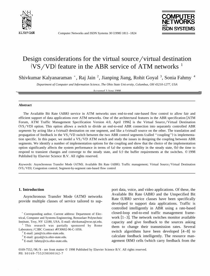
Fig. 4. Multiple unidirectional VCs in a VSVD switch.

Žon the same segment as specified in the destinationw x.end system rules 2 . Additionally, when the FRM

cells are turned around, the switch may decrease theŽ .value of the explicit rate ER field to account for the

bottleneck rate of the next link and the ER from thesubsequent ABR segments.

When the VS at the next loop receives a BRMcell, the ACR of the per-VC queue at the VS is

Župdated using the ER field in the BRM ER of the.subsequent ABR segments as specified in the source

w x.end system rules 2 . Additionally, the ER value ofthe subsequent ABR segments needs to be madeknown to the VD of the first segment. One way ofdoing this is for the VD of the first segment to usethe ACR of the VC in the VS of the next segmentwhile turning around FRM cells.

The model can be extended to multiple unidirec-tional VCs in a straightforward way. Fig. 4 showstwo unidirectional VCs, VC1 and VC2, between thesame source S and destination D which go from

Link1 to Link2 on a VSrVD switch. Observe thatthere is a separate VS and VD control for each VC.We omit non-ABR queues in this and subsequentfigures.

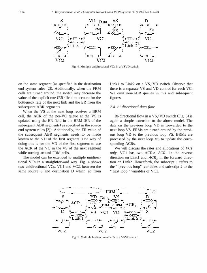
2.4. Bi-directional data flow

Ž .Bi-directional flow in a VSrVD switch Fig. 5 isagain a simple extension to the above model. Thedata on the previous loop VD is forwarded to thenext loop VS. FRMs are turned around by the previ-ous loop VD to the previous loop VS. BRMs areprocessed by the next loop VS to update the corre-sponding ACRs.

We will discuss the rates and allocations of VC1only. VC1 has two ACRs: ACR in the reverse1

direction on Link1 and ACR in the forward direc-2

tion on Link2. Henceforth, the subscript 1 refers tothe ‘‘previous loop’’ variables and subscript 2 to the‘‘next loop’’ variables of VC1.

Fig. 5. Multiple bi-directional VCs in a VSVD switch.

( )S. Kalyanaraman et al.rComputer Networks and ISDN Systems 30 1998 1811–1824 1815

3. Basic ERICA switch scheme

w xWe use basic version of the ERICA algorithm 8for congestion control at the switches. We give abrief overview of the algorithm in this section. Notethat the full ERICA algorithm contains several en-hancements which account for fairness, queueingdelays, and which handles highly variant burstyŽ .ON-OFF traffic efficiently. A complete descriptionof the algorithm with proofs of fairness and perfor-

w xmance is provided in 8 .ERICA first sets a target rate as follows:

Target RatesTarget Utilization=Link Rate

yVBR RateyCBR Rate.

It also measures the input rate to the ABR queueand the number of active ABR sources.

Ž .To achieve fairness, the VC’s Allocation VAhas a component:

VA sTarget RaterNumber of Active VCs.fairness

Ž .To achieve efficiency, the VC’s Allocation VAhas a component:

VA s VC’s Current Cell Ratereffic iency

Overload, where Overload s Input RaterTargetRate.

Ž .Finally, the VC’s allocation on this link VAL iscalculated as:

VALsMax VA ,VA� 4efficiency fairness

� 4sFunction Input Rate, VC’s Current Rate .

We now describe the points where the ERICArate calculations are done in a non-VSrVD switchand in a VSrVD switch.

3.1. Rate calculations in a non-VSrVD switch

Ž .The non-VSrVD switch calculates the rate VALfor sources when the BRMs are processed in thereverse direction and enters it in the BRM field asfollows:

� 4ER in BRMsMin ER in BRM, VAL .At the source end system, the ACR is updated as:

� 4ACRsFunction ER, VC’s Current ACR .

3.2. Rate calculations in a VSrVD switch

Fig. 6 shows the rate calculations in a VSrVDswitch. Specifically, the segment starting at Link2Ž .‘‘next loop’’ returns an ER value, ER in the2

ŽBRM, and the FRM of the first segment ‘‘previous.loop’’ is turned around with an ER value of ER .1

The ERICA algorithm for the port to Link2 calcu-Ž . �lates a rate VAL as: VAL sFunction Input Rate,2 2

4VC’s Current Rate . The rate calculations at the VSand VD are as follows:Ø Destination algorithm for the preÕious loop: ER1

� 4sMin ER ,VAL , ACR .1 2 2

Ø Source algorithm for the next loop: Optionally,� 4E R s M in E R ,V A L , A C R s F n2 2 2 2

� 4ER , ACR .2 2

The unknowns in the above equations are theinput rate and the VC’s current rate. We shall see inthe next section that there are several ways of mea-suring VC rates and input rates, combining the feed-back from the next loop, and updating the ACR ofthe next loop. Note that though different switchesmay implement different algorithms, many measurequantities such as the VC’s current rate and the ABRinput rate.

Fig. 6. Rate calculations in VSrVD switches.

( )S. Kalyanaraman et al.rComputer Networks and ISDN Systems 30 1998 1811–18241816

4. VSrrrrrVD switch design options

In this section, we aim at answering the followingquestions:

Ž .Ø What is a VC’s current rate? 4 optionsŽ .Ø What is the input rate? 2 options

Ø Does the congestion control actions at a linkŽaffect the next loop or the previous loop? 3

.optionsŽ .Ø When is the VC’s allocation at the link VAL

Ž .calculated? 3 optionsŽ .We will enumerate the 72 s 4 = 2 = 3 = 3

option combinations and then study this state spacefor the best combination.

4.1. Measuring the VC’s current rate

There are four methods to measure the VC’scurrent rate:1. The rate of the VC is declared by the source end

system of the previous loop in the Current CellŽ . Ž .Rate CCR field of the FRM cell FRM1 re-

ceived by the VD. This declared value can beused as the VC’s rate.

2. The VS to the next loop declares the CCR valueŽ . Ž .of the FRM sent FRM2 to be its ACR ACR .2

This declared value can be used as the VC’s rate.3. The actual source rate in the preÕious loop can

be measured. This rate is equal to the VC’s inputrate to the per-VC queue. This measured sourcerate can be used as the VC’s rate.

4. The actual source rate in the next loop can bemeasured as the VC’s input rate to the per-class

Ž .queue from the per-VC queue . This measuredvalue can be used as the VC’s rate.Fig. 7 illustrates where each method is applied

Ž .note the position of the numbers in circles .

4.2. Measuring the input rate at the switch

Ž .Fig. 8 note the position of the numbers in circlesshows two methods of estimating the input rate foruse in the switch algorithm calculations. These twomethods are:1. The input rate is the sum of input rates to the

per-VC ABR queues.2. The input rate is the aggregate input rate to the

per-class ABR queue.

4.3. Effect of link congestion actions on neighboringlinks

The link congestion control actions can affectneighboring links. The following actions are possiblein response to the link congestion of Link2:1. Change ER . This affects the rate of the preÕious1

loop only. The change in rate is experienced onlyafter a feedback delay equal to twice the propaga-tion delay of the loop.

2. Change ACR . This affects the rate of the next2

loop only. The change in rate is experiencedinstantaneously.

3. Change ER and ACR . This affects both the1 2

preÕious and the next loop. The next loop isaffected instantaneously while the previous loopis affected after a feedback delay as in the firstcase.

4.4. Frequency of updating the allocated rate

The ERICA algorithm in a non-VSrVD switchcalculates the allocated rate when a BRM cell is

Fig. 7. Four methods to measure the rate of a VC at the VSrVD switch.

( )S. Kalyanaraman et al.rComputer Networks and ISDN Systems 30 1998 1811–1824 1817

Fig. 8. Two methods to measure the input rate at the VSrVD switch.

processed in a switch. However, in a VSrVD switch,there are three options as shown in Fig. 9:1. Calculate allocated rate on receiÕing BRM2 only.

Store the value in a table and use this table valuewhen an FRM is turned around.

2. Calculate allocated rate only when FRM1 is turnedaround.

3. Calculate allocated rate both when FRM1 is turnedaround as well as when BRM2 is receiÕed.In the next section, we discuss the various options

and present analytical arguments to eliminate certaindesign combinations.

5. VSrrrrrVD switch design options

5.1. VC rate measurement techniques

We have presented four ways of finding the theVC’s current rate in Section 4.1, two of them useddeclared rates and two of them measured the actualsource rate. We show that measuring source rates isbetter than using declared rates for two reasons.

First, the declared VC rate of a loop naively is theminimum of bottleneck rates of downstream loopsonly. It does not consider the bottleneck rates ofupstream loops, and may or may not consider thebottleneck rate of the first link of the next loop.Measurement allows better estimation of load whenthe traffic is not regular.

Second, the actual rate of the VC may be lowerthan the declared ACR of the VC due to dynamicchanges in bottleneck rates upstream of the currentswitch. The difference in ACR and VC rate willremain at least as long as the time required for newfeedback from the bottleneck in the path to reach thesource plus the time for the new VC rate to beexperienced at the switch. The sum of these twodelay components is called the ‘‘feedback delay.’’Due to feedback delay, it is possible that the declaredrate is a stale value at any point of time. This isespecially true in VSrVD switches where per-VCqueues may control source rates to values quitedifferent from their declared rates.

Further, the measured source rate can easily becalculated in a VSrVD switch since the necessary

Fig. 9. Three methods to update the allocated rate.

( )S. Kalyanaraman et al.rComputer Networks and ISDN Systems 30 1998 1811–18241818

Fig. 10. Two adjacent loops may operate at very different rates forone feedback delay.

Ž .quantities number of cells and time period aremeasured as part of one of the source end system

Ž . w xrules SES Rule 5 1,2,10 .

5.2. Input rate measurement techniques

As discussed earlier, the input rate can be mea-sured as the sum of the input rates of VCs to theper-VC queues or the aggregate input rate to theper-class queue. These two rates can be differentbecause the input rate to the per-VC queues is at theprevious loop’s rate while the input to the per-classqueue is related to the next loop’s rate. Fig. 10shows a simple case where two adjacent loops can

Ž .run at very different rates 10 Mbps and 100Mbpsfor one feedback delay.

5.3. Combinations of VC rate and input rate mea-surement options

Table 1 summarizes the option combinations con-sidering the fact that two adjacent loops may run atdifferent rates. The table shows that four of thesecombinations may work satisfactorily. The othercombinations use inconsistent information and hencemay either overallocate rates leading to uncon-strained queues or result in unnecessary oscillations.

We can eliminate some more cases as discussedbelow.

Table 1 does not make any assumptions about theŽqueue lengths at any of the queues per-VC or

.per-class . For example, when the queue lengths areclose to zero, the actual source rate might be muchlower than the declared rate in the FRMs leading tooverallocation of rates. This criterion can be used toreject more options.

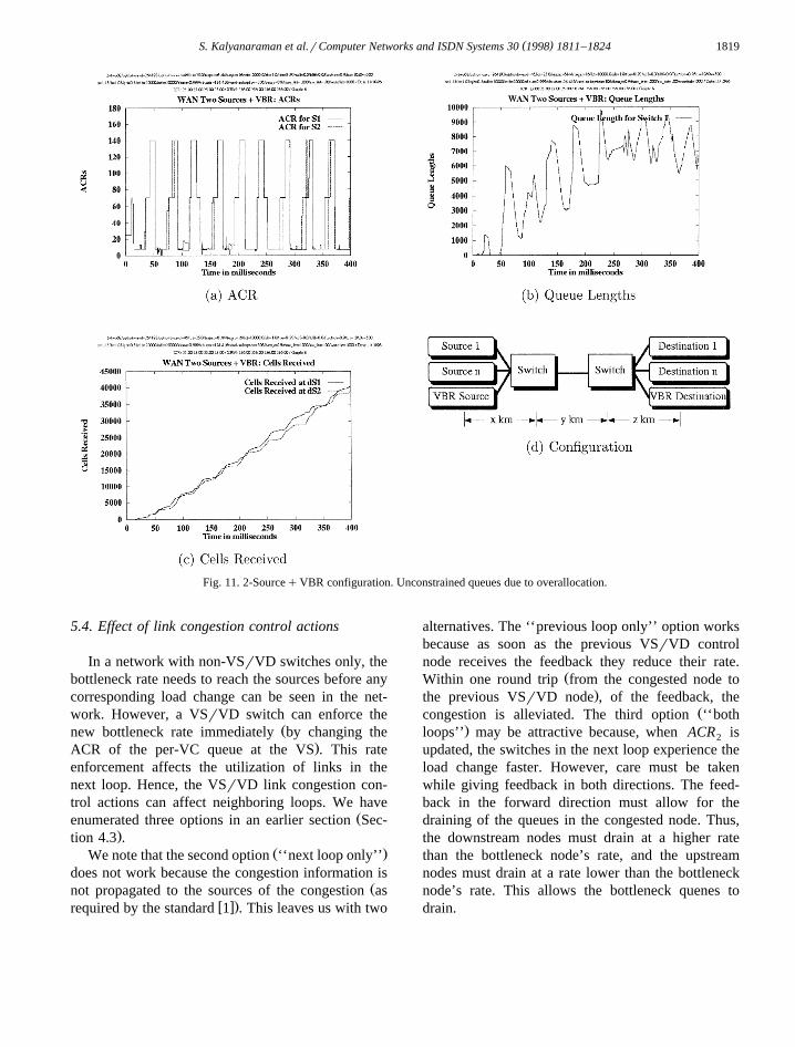
The performance of one such rejected case isŽshown in Fig. 11 corresponding to row 4 in Table

.1 . The fine print in the figures depicting graphs canŽbe ignored for the purposes of this discussion they

.are parameter values specific to the simulator used .The configuration used has two ABR infinite sourcesand one high priority VBR source contending for the

Ž .bottleneck link’s LINK1 bandwidth. The VBR hasan ONrOFF pattern, where it uses 80% of the linkcapacity when ON. The ON time and the OFF time

Ž .are equal 20 ms each . The VSrVD switch overal-locates rates when the VBR source is OFF. Thisleads to ABR queue backlogs when the VBR sourcecomes ON in the next cycle. The queue backlogs arenever cleared, and hence the queues diverge. In thiscase, the fast response of VSrVD is harmful be-cause the rates are overallocated.

In this study, we have not evaluated row 5 of theŽtable measurement of VC rate at entry to the per-VC.queues . Hence, out of the total of 8 combinations,

we consider two viable combinations: row 1 and row8 of the table. Note that since row 8 uses source ratemeasurement, we expect it to show better perfor-mance. This is substantiated by our simulation re-sults presented later in the paper.

Table 1Viable combinations of VC rate and input rate measurement

Row a VC rate method Ý VC rates Input rate Input rate DesignŽ . Ž .Mbps method value YESrNO

1. From FRM1 10 Ý per-VC 10 YES2. From FRM1 10 per-class 10-100 NO3. From FRM2 100 Ý per-VC 10 NO4. From FRM2 100 per-class 100 YES5. At per-VC queue 10 Ý per-VC 10 YES6. At per-VC queue 10 per-class 10-100 NO7. At per-class queue 100 Ý per-VC 10 NO8. At per-class queue 100 per-class 100 YES

( )S. Kalyanaraman et al.rComputer Networks and ISDN Systems 30 1998 1811–1824 1819

Fig. 11. 2-SourceqVBR configuration. Unconstrained queues due to overallocation.

5.4. Effect of link congestion control actions

In a network with non-VSrVD switches only, thebottleneck rate needs to reach the sources before anycorresponding load change can be seen in the net-work. However, a VSrVD switch can enforce the

Žnew bottleneck rate immediately by changing the.ACR of the per-VC queue at the VS . This rate

enforcement affects the utilization of links in thenext loop. Hence, the VSrVD link congestion con-trol actions can affect neighboring loops. We have

Ženumerated three options in an earlier section Sec-.tion 4.3 .

Ž .We note that the second option ‘‘next loop only’’does not work because the congestion information is

Žnot propagated to the sources of the congestion asw x.required by the standard 1 . This leaves us with two

alternatives. The ‘‘previous loop only’’ option worksbecause as soon as the previous VSrVD controlnode receives the feedback they reduce their rate.

ŽWithin one round trip from the congested node to.the previous VSrVD node , of the feedback, the

Žcongestion is alleviated. The third option ‘‘both.loops’’ may be attractive because, when ACR is2

updated, the switches in the next loop experience theload change faster. However, care must be takenwhile giving feedback in both directions. The feed-back in the forward direction must allow for thedraining of the queues in the congested node. Thus,the downstream nodes must drain at a higher ratethan the bottleneck node’s rate, and the upstreamnodes must drain at a rate lower than the bottlenecknode’s rate. This allows the bottleneck quenes todrain.

( )S. Kalyanaraman et al.rComputer Networks and ISDN Systems 30 1998 1811–18241820

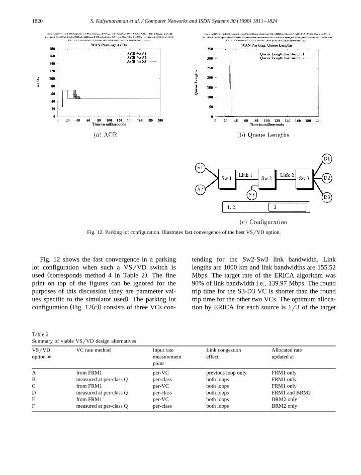
Fig. 12. Parking lot configuration. Illustrates fast convergence of the best VSrVD option.

Fig. 12 shows the fast convergence in a parkinglot configuration when such a VSrVD switch is

Ž .used corresponds method 4 in Table 2 . The fineprint on top of the figures can be ignored for the

Žpurposes of this discussion they are parameter val-.ues specific to the simulator used . The parking lot

Ž Ž ..configuration Fig. 12 c consists of three VCs con-

tending for the Sw2-Sw3 link bandwidth. Linklengths are 1000 km and link bandwidths are 155.52Mbps. The target rate of the ERICA algorithm was90% of link bandwidth i.e., 139.97 Mbps. The roundtrip time for the S3-D3 VC is shorter than the roundtrip time for the other two VCs. The optimum alloca-tion by ERICA for each source is 1r3 of the target

Table 2Summary of viable VSrVD design alternatives

VSrVD VC rate method Input rate Link congestion Allocated rateoption a measurement effect updated at

point

A from FRM1 per-VC previous loop only FRM1 onlyB measured at per-class Q per-class both loops FRM1 onlyC from FRM1 per-VC both loops FRM1 onlyD measured at per-class Q per-class both loops FRM1 and BRM2E from FRM1 per-VC both loops BRM2 onlyF measured at per-class Q per-class both loops BRM2 only

( )S. Kalyanaraman et al.rComputer Networks and ISDN Systems 30 1998 1811–1824 1821

Fig. 13. Link congestion and allocated rate update: viable options.

Ž . Ž .rate on the Sw2-Sw3 about 46.7 Mbps . Fig. 12 ashows that the optimum value is reached at 40 ms.

Ž .Part b of the figure shows that the transient queuesare small and that the allocation is fair.

5.5. Link congestion and allocated rate update fre-quency: Õiable options

Ž .The allocated rate update has three options: aŽ .update upon BRM receipt in VS and enter the

value in a table to be used when an FRM is turnedŽ . Ž .around, b update upon FRM turnaround at VD

Ž . Ž .and no action at VS, c update both at FRM VDŽ .and at BRM VS without use of a table.

The last option recomputes the allocated rate alarger number of times, but can potentially allocaterates better because we always use the latest infor-mation.

The allocated rate update and the effects of linkcongestion actions interact as shown in Fig. 13. Thefigure shows a tree where the first level considers the

Ž .link congestion 2 options , i.e., whether the nextloop is also affected or not. The second level lists thethree options for the allocated rate update frequency.The viable options are those highlighted in bold atthe leaf level.

Other options are not viable because of the fol-lowing reasons. In particular, if the link congestiondoes not affect the next loop, the allocated rateupdate at the FRM turnaround is all that is required.The allocated rate at the BRM is redundant in thiscase. Further, if the link congestion affects the nextloop, then the allocated rate update has to be done onreceiving a BRM, so that ACR can be changed at theVS. This gives us two possibilities as shown in the

Ž .figure BRM only, and BRMqFRM .Hence, we have three viable combinations of link

congestion and the allocated rate update frequency.A summary of all viable VSrVD implementation

Ž .options a total of 6, coded as A through F is listedin Table 2.

The next section evaluates the performance of theviable VSrVD design options through simulation.

6. Performance evaluation of VSrrrrrVD design op-tions

6.1. Metrics

We use four metrics to evaluate the performanceof these alternatives:Ø Response Time: is the time taken to reach near

optimal behavior on startup.Ø ConÕergence Time: is the time for rate oscilla-

Ž .tions to decrease time to reach the steady state .Ø Throughput: Total data transferred per unit time.Ø Maximum Queue: The maximum queue before

convergence.The difference between response time and conver-

gence time is illustrated in Fig. 14. The followingsections present simulation results with respect to the

Žabove metrics. Note that we have used greedy in-.finite traffic sources in our simulations. We have

studied the algorithmic enhancements in non-VSrVDw xswitches for non-greedy sources in 8 . We expect

consistent results for such traffic when the bestŽ .implementation option see below is used.

6.1.1. Response timeWithout VSrVD all response times are close to

the round-trip delay. With VSrVD, the responsetimes are close to the feedback delay from thebottleneck. Since VSrVD reduces the response timeduring the first round trip, it is good for long delay

Žpaths. The quick response time 10 ms in the parking.lot configuration which has a 30 ms round trip time

was illustrated previously in Fig. 12.

Fig. 14. Response time versus convergence time.

( )S. Kalyanaraman et al.rComputer Networks and ISDN Systems 30 1998 1811–18241822

Response time is also important for bursty trafficlike TCP file transfer over ATM which ‘‘starts up’’

Žat the beginning of every active period when the.TCP window increases after the corresponding idle

w xperiod 9,10 .

6.1.2. ThroughputThe number of cells received at the destination is

a measure of the throughput achieved. These valuesare listed in Table 3. The top row is a list of the

ŽVSrVD implementation option codes these codes.are explained in Table 2, first column . The final

column lists the throughput values for the case whena non-VSrVD switch is used. The 2 sourceqVBRand the parking lot configurations have been intro-duced in earlier section.

The upstream bottleneck configuration shown inFig. 15 has a bottleneck at Sw1 where 15 VCs sharethe Sw1-Sw2 link. As a result the S15-D15 VC isnot capable of utilizing its bandwidth share at theSw2-Sw3 link. This excess bandwidth needs to beshared equally by the other two VCs. The table entryshows the number of cells received at the destinationfor either the S16-D16 VC or the S17-D17 VC.

In the 2 sourceqVBR and the upstream bottle-neck configurations, the simulation was run for 400

Žms the destination receives data from time s 15.ms through 400 ms . In the parking lot configuration,

the simulation was run for 200 ms.As we compare the values in each row of the

table, we find that, in general, there is little differ-ence between the alternatiÕes in terms of throughput.However, there is a slight increase in throughputwhen VSrVD is used over the case without VSrVDswitch.

6.1.3. ConÕergence timeThe convergence time is a measure of how fast

the scheme finishes the transient phase and reachessteady state. It is also sometimes called ‘‘transient

Table 3Cells received at the destination per source in Kcells

VSrVD option a ™ A B C D E F No.VSrVDConfiguration x

2 source q VBR 31 31 32.5 34 32 33 30Parking lot 22 22 23 20.5 23 20.5 19.5Upstream bottleneck 61 61 61 60 61 61 62

Fig. 15. Upstream bottleneck configuration.

response’’. The convergence times of the variousoptions are shown in Table 4. The ‘‘transient’’ con-figuration mentioned in the table has two ABR VCs

Žsharing a bottleneck like the 2 source q VBR.configuration, but without the VBR VC . One of the

VCs comes on in the middle of the simulation andremains active for a period of 60 ms before goingoff.

Observe that the convergence time of VSrVDŽ . Žoption D highlighted is the best. Recall see Table

.2 that this configuration corresponds to measuringthe VC rate at the entry to the per-class queue, inputrate measured at the per-class queue, link congestionaffecting both the next loop and the previous loop,the allocated rate updated at both FRM1 and BRM2.

6.1.4. Maximum transient queue lengthThe maximum transient queues gives a measure

of how askew the allocations were when comparedto the optimal allocation and how soon this wascorrected. The maximum transient bottleneck queuesare tabulated for various configurations for eachVSrVD option and for the case without VSrVD inTable 5. The bottleneck in the parking lot and up-stream configurations is the port in switch 2 connect-ing to Link 2. The bottleneck in the 2 source qVBR and transient configuration is the port in switch1 connecting to link 1.

Table 4Convergence time in ms.

VSrVD option a ™ A B C D E F No.VSrVDConfiguration x

Transient 50 50 65 20 55 25 60Parking lot 120 100 170 45 125 50 140Upstream bottleneck 95 75 75 20 95 20 70

( )S. Kalyanaraman et al.rComputer Networks and ISDN Systems 30 1998 1811–1824 1823

Table 5Maximum bottleneck queue length in Kcells

VSrVD option a ™ A B C D E F No.VSrVDConfiguration x

2 Source q VBR 1.2 1.4 2.7 1.8 2.7 1.8 2.7Transient 1.4 1.1 1.4 0.025 1.3 1.0 6.0Parking lot 1.9 1.9 1.4 0.3 3.7 0.35 2.0Upstream bottleneck 0.025 0.08 0.3 0.005 1.3 0.005 0.19

The table shows that VSrVD option D has verysmall transient queues in all the configurations andthe minimum queues in a majority of cases. Thisresult, combined with the fastest response and near-maximum throughput behavior confirms the choiceof option D as the best VSrVD implementation.

Observe that the queues for the VSrVD imple-mentations are in general lesser than or equal to thequeues for the case without VSrVD. However, thequeues reduce much more if the correct implementa-

Ž .tion like option D is chosen.

7. Conclusions

In summary:Ø VSrVD is an option that can be added to switches

which implement per-VC queueing. The additioncan potentially yield improved performance interms of response time, convergence time, andsmaller queues. This is especially useful forswitches at the edge of satellite networks orswitches that are attached to links with largedelay-bandwidth product. The fast response andconvergence times also help support bursty trafficŽ .eg: data traffic more efficiently.

Ø The effect of VSrVD depends upon the switchalgorithm used and how it is implemented in theVSrVD switch. The convergence time and tran-sient queues can be very different for differentVSrVD implementations of the same basic switchalgorithm. In such cases the fast response ofVSrVD is harmful.

Ø With VSrVD, ACR and actual rates are verydifferent. The switch cannot rely on the RM cellCCR field. We recommend that the VSrVDswitch and in general, switches implementing per-

VC queueing measure the VC’s current rate.Ø The sum of the input rates to per-VC VS queues

is not the same as the input rate to the link. It isbest to measure the VC’s rate at the output of theVS and the input rate at the entry to the per-classqueue.

Ø On detecting link congestion, the congestion in-formation must be forwarded to the previous loopand may be also forwarded to the next loop.

Ž .However, in forwarding to the next downstreamloop, the bottleneck queues should be allowed todrain. As a result, the previous loop must begiven feedback lower than the bottleneck’s drainrate, and the next hop must drain at a rate higherthan the bottleneck’s drain rate. This methodreduces the convergence time by reducing thenumber of iterations required in the switch algo-rithms on the current and downstream switches.

Ø It is best for the rate allocated to a VC to becalculated both when turning around FRMs at theVD as well as after receiving BRMs at the nextVS.

8. Future work

The VSrVD provision in the ABR traffic man-agement framework can potentially improve perfor-mance of bursty traffic and reduce the buffer require-ments in switches. The VSrVD mechanism achievesthis by breaking up a large ABR loop into smallerABR loops which are separately controlled. How-ever, further study is required in the following areas:Ø Effect of VSrVD on buffer requirements in the

switch.Ø Scheduling issues with VSrVD.Ø Effect of different switch algorithms in different

control loops, and different control loop lengths.Ø Effect of non-ABR clouds and standardization

issues involved.Ø Effect of using switch algorithms specifically de-

signed to exploit the per-VC queueing policyrequired in VSrVD implementations.

References

w x1 ATM Forum, ATM Traffic Management Specification Ver-sion 4.0, April 1996, available as ftp:rrftp.atmforum.comrpubrapproved-specsraf-tm-0056.000.ps

( )S. Kalyanaraman et al.rComputer Networks and ISDN Systems 30 1998 1811–18241824

w x2 R. Jain, S. Kalyanaraman, R. Goyal, S. Fahmy, Sourcebehavior for ATM ABR traffic management: an explanation,

Ž . ŽIEEE Communications Magazine November 1996 . All ourpapers and ATM Forum contributions are available through

.http:rrwww.cis.ohio-state.edur; jain.w x3 K. Fendick, Evolution of controls for the available bit rate

Ž .service, IEEE Communications Magazine November 1996 .w x Ž4 L. Roberts, Enhanced PRCA Proportional Rate-Control Al-

.gorithm , AF-TM 94-0735R1, August 1994.w x5 K. Siu and T. Tzeng, Intelligent congestion control for ABR

service in ATM networks, Computer Communication ReviewŽ .24 1995 81.

w x6 L. Kalampoukas, A. Varma, K.K. Ramakrishnan, An effi-cient rate allocation algorithm for ATM networks providingmax-min fairness, Proc. 6th IFIP Int. Conf. on High Perfor-mance Networking, September 1995.

w x7 Y. Afek, Y. Mansour, Z. Ostfeld, Phantom: a simple andeffective flow control scheme, Proc. ACM SIGCOMM, Au-gust 1996.

w x8 S. Kalyanaraman, R. Jain, S. Fahmy, R. Goyal, B. Van-dalore, The ERICA switch algorithm for ABR traffic man-agement in ATM networks, IEEE Transactions on Network-ing, submitted.

w x9 A. Charny, G. Leeb, M. Clarke, Some observations on sourcebehavior 5 of the traffic management specification, AF-TM95-0976R1, August 1995.

w x10 S. Kalyanaraman, R. Jain, S. Fahmy, R. Goyal, Use-it-or-Ž .lose-it policies for the available bit rate ABR service in

ATM networks, Computer Networks and ISDN Systems, toappear.

Shivkumar Kalyanaraman is an Assistant Professor at the De-partment of Electrical, Computer and Systems Engineering atRensselaer Polytechnic Institute in Troy, NY. He received aB.Tech degree from the Indian Institute of Technology, Madras,India in July 1993, followed by M.S. and and Ph.D. degrees inComputer and Information Sciences at the Ohio State Universityin 1994 and 1997, respectively. His research interests includemultimedia networking, Internet and ATM traffic management,Internet pricing, and performance analysis of distributed systems.

ŽHe is a co-inventor in two patents the ERICA and OSU schemes.for ATM traffic management , and has co-authored papers, ATM

forum contributions and IETF drafts in the field of ATM andInternet traffic management. He is a member of IEEE-CS andACM. His publications may be accessed through http:rrwww.ecse.rpi.edurHomepagesrshivkuma.

Raj Jain is a Professor of Computer and Information Science atThe Ohio State University in Columbus, OH. He is very active inthe Traffic Management working group of ATM Forum and hasinfluenced its direction considerably. He received a Ph.D. degreein Computer Science from Harvard in 1978 and is the author of‘‘Art of Computer Systems Performance Analysis,’’ Wiley, 1991,and ‘‘FDDI Handbook: High-Speed Networking with Fiber andOther Media,’’ Addison-Wesley, 1994. Dr. Jain is an IEEE Fel-low, an ACM Fellow, and is on the Editorial Boards of Computer

Ž .Networks and ISDN Systems, Computer Communications UK ,Ž .Journal of High Speed Networking USA , and Mobile Networks

Ž .and Nomadic Applications NOMAD . For his publications, pleasesee http:rrwww.cis.ohio-state.edur; jain.

Rohit Goyal is a Ph.D. candidate and a Presidential Fellow withthe Department of Computer and Information Science at the OhioState University, Columbus. He received his Bachelor of Sciencein Computer Science from Denison University, Granville, and hisMaster of Science in Computer and Information Science from TheOhio State University. His research interests are in the area oftraffic management and quality of service for high speed net-works. His recent work has been in buffer management for UBRand GFR, QoS scheduling, feedback control for ABR, and TCPrIPover ATM for terrestrial and satellite networks. His other interestsinclude distributed systems and artificial intellitence. Internet:http:rrwww.cis.ohio-state.edur;goyal.

Sonia Fahmy received her B.Sc. degree from the AmericanUniversity in Cairo, Egypt, in June 1992, and her M.S. degreefrom the Ohio State University in March 1996, both in ComputerScience. She is currently a Ph.D. student at the Ohio StateUniversity. Her main research interests are in the areas of broad-band networks, multipoint communication, traffic management,performance analysis, and distributed computing. She is the authorof several papers and ATM Forum contributions. She is a studentmember of the ACM and the IEEE Computer and Communica-tions societies. Internet: http:rrwww.cis.ohio-state.edur ;

fahmy.