Page 1
Design decision alternatives for agent-based monitoring of distributed server
environments
Einar Sveinsson
Faculty of Industrial Engineering, Mechanical Engineering and
Computer Science
University of Iceland 2012
Page 3
Design decision alternatives for agent-based monitoring of distributed server
environments
Einar Sveinsson
60 ECTS thesis submitted in partial fulfillment of a
Magister Scientiarum degree in Software Engineering
Advisor(s) Helmut Wolfram Neukirchen
Snorri Agnarsson
Faculty Representative Jóhann Pétur Malmquist
Faculty of Industrial Engineering, Mechanical Engineering and Computer Science
School of Engineering and Natural Sciences University of Iceland
Reykjavik, October 2012
Page 4
Design decision alternatives for agent-based monitoring of distributed server environments
60 ECTS thesis submitted in partial fulfillment of a Magister Scientiarum degree in
Software Engineering
Copyright © 2012 Einar Sveinsson
All rights reserved
Faculty of Industrial Engineering, Mechanical Engineering and Computer Science
School of Engineering and Natural Sciences
University of Iceland
Hjarðarhaga 2-6
107, Reykjavik
Iceland
Telephone: 525 4000
Bibliographic information:
Einar Sveinsson, 2012, Design decision alternatives for agent-based monitoring of
distributed server environments, Master’s thesis, Faculty of Industrial Engineering,
Mechanical Engineering and Computer Science, University of Iceland.
Printing: Háskólaprent, Fálkagata 2, 107 Reykjavík
Reykjavik, Iceland, October 2012
Page 5
Abstract
In every IT department it is crucial for the management to be able to have a good overview
of their service infrastructure to be able to charge for their service operation cost. With
distributed services that do not always run on dedicated servers many services can be
located on the same server and therefore it is needed to split the operation cost between the
services. To be able to split this cost in a correct way a lot of information needs to be
available, such as the resource usage and audit information for the systems so the cost for
the system can be divided between the users.
In this thesis are two design alternatives for agent frameworks developed and evaluated to
see if it possible to create more accurate cost model by either of them using agents to
monitor the service located on servers.
Page 6
Útdráttur
Fyrir allar UT deildir í fyrirtækjum er mjög mikilvægt fyrir stjórnendur deildarinnar að
hafa góða yfirsýn yfir þær þjónustur sem deildin er að bjóða upp á og hverjir eru að nota
þær. Þessar upplýsingar eru mikilvægar ef rukka þarf aðrar deildir fyrir rekstarkostnað t.d.
á serverum ofl..
Í þessari ritgerð eru tvær útgáfur af milliliða ramma(e. agent framework) búnar til og
út frá þeim eru búnir til milliliðir sem sjá um að fylgjast með notkun á þjónustum sem og
hversu mikið af miðverkinu (e. central processing unit) og innra minninu þjónusturnar eru
að nota. Bornar eru saman þessar tvær útgáfur og séð hver af þeim getur búið til
nákvæmari gögn sem sýna rétt mynd af notkun þjónustanna. Þessar upplýsingar eru síðan
notaðar til að reyna búa til nákvæmt kostnaðar líkan fyrir útskuldun á þjónustum.
Page 7
Dedicated to my family
I could never do this without you!
Page 9
Table of Contents
List of Figures ...................................................................................................................... x
List of Tables ..................................................................................................................... xiii
Abbreviations .................................................................................................................... xiv
Acknowledgements .......................................................................................................... xvii
1 Introduction ..................................................................................................................... 1 1.1 Problem ................................................................................................................... 1 1.2 Approach ................................................................................................................. 1 1.3 Outline of thesis....................................................................................................... 2
2 Foundations ..................................................................................................................... 5 2.1 Agents ...................................................................................................................... 5
2.2 FIPA ........................................................................................................................ 6 2.2.1 Agent Management ........................................................................................ 7
2.2.2 Agent Message Transport .............................................................................. 9 2.3 Python .................................................................................................................... 10
2.3.1 PSUTIL ........................................................................................................ 11
2.3.2 Twisted ......................................................................................................... 11 2.3.3 PYODBC ..................................................................................................... 12
2.4 SQL ....................................................................................................................... 12 2.4.1 Microsoft SQL Server .................................................................................. 13 2.4.2 Microsoft SQL Server Integration Service .................................................. 13
3 Related work ................................................................................................................. 15 3.1 Agent Frameworks ................................................................................................ 15
3.1.1 JADE framework ......................................................................................... 15
3.1.2 Spade ............................................................................................................ 17 3.2 Monitoring ............................................................................................................. 17
3.2.1 System Center Operation Manager .............................................................. 17
4 Cost Model ..................................................................................................................... 19 4.1 Purpose of the Cost Model .................................................................................... 19
4.2 Basics of the Cost Model....................................................................................... 19
5 Agent Framework ......................................................................................................... 21 5.1 Container ............................................................................................................... 21
5.1.1 Types ............................................................................................................ 21 5.1.2 Message Manager ........................................................................................ 25 5.1.3 Time dispatcher ............................................................................................ 28
5.2 Behaviour .............................................................................................................. 29
Page 10
viii
5.2.1 Types ........................................................................................................... 30 5.2.2 System behaviours ....................................................................................... 31
5.3 Framework Agents ................................................................................................. 32 5.3.1 Types ........................................................................................................... 32
5.3.2 Lifecycle ...................................................................................................... 33 5.3.3 Scheduler ..................................................................................................... 35 5.3.4 Data storage ................................................................................................. 35
6 Agents ............................................................................................................................. 37 6.1 Functionality .......................................................................................................... 37
6.2 Behaviour ............................................................................................................... 37
6.2.1 InitialProcessBehaviour ............................................................................... 38
6.2.2 ProcessBehaviour ........................................................................................ 38 6.2.3 MemoryBehaviour ....................................................................................... 39 6.2.4 ProcessorBehaviour ..................................................................................... 39 6.2.5 SQLBehaviour ............................................................................................. 40 6.2.6 ConnectionMonitorBehaviour ..................................................................... 40
6.2.7 SniffingBehaviour ....................................................................................... 41
7 Post processing ............................................................................................................... 43 7.1 Database structure .................................................................................................. 43 7.2 Data processing ...................................................................................................... 44
8 Evaluation ...................................................................................................................... 47 8.1 Evaluation Environment ........................................................................................ 47
8.1.1 Client ........................................................................................................... 48 8.1.2 File Service .................................................................................................. 49
8.1.3 String Service .............................................................................................. 49 8.1.4 Test Environment Configuration ................................................................. 49 8.1.5 Monitoring ................................................................................................... 50
8.2 Agent Framework Setups ....................................................................................... 50 8.2.1 Standard Framework Setup ......................................................................... 50
8.2.2 Changed Framework Setup ......................................................................... 51 8.3 Memory Results ..................................................................................................... 53
8.3.1 Scenario 1 .................................................................................................... 53 8.3.2 Scenario 1 - run 2 ......................................................................................... 55 8.3.3 Scenario 2 .................................................................................................... 58 8.3.4 Scenario 2 - run 2 ......................................................................................... 60 8.3.5 Scenario 3 .................................................................................................... 63
8.3.6 Scenario 3 - run 2 ......................................................................................... 65 8.4 CPU Results ........................................................................................................... 67
8.4.1 Scenario 1 .................................................................................................... 67 8.4.2 Scenario 1 - run 2 ......................................................................................... 70 8.4.3 Scenario 2 .................................................................................................... 72
8.4.4 Scenario 2 - run 2 ......................................................................................... 75
8.4.5 Scenario 3 .................................................................................................... 77
8.4.6 Scenario 3 - run 2 ......................................................................................... 79 8.5 Network Results ..................................................................................................... 82 8.6 Conclusion ............................................................................................................. 92
Page 11
ix
9 Summary and outlook .................................................................................................. 94
References........................................................................................................................... 97
Page 12
x
List of Figures
Figure 2.1.1 A Part View of an Agent Typology [2] ............................................................ 6
Figure 2.2.1 Structure of FIPA Specifications [4] ................................................................ 7
Figure 2.2.2 Agent Management Reference Model [5] ........................................................ 7
Figure 2.2.3 FIPA agent life cycle [5] ................................................................................... 9
Figure 2.2.4 Message Transport Reference Model [6] ........................................................ 10
Figure 3.1.1 The JADE Architecture [23] ........................................................................... 16
Figure 3.1.2 UML Model of the JADE Behaviour class hierarchy [24] ............................. 16
Figure 3.1.3 Spade overview [25] ....................................................................................... 17
Figure 5.1.1 The Agent framework on N servers ................................................................ 22
Figure 5.1.2 Agent container ............................................................................................... 24
Figure 5.1.3 Domain Container ........................................................................................... 25
Figure 5.1.4 TimeDispatcher Activity diagram .................................................................. 29
Figure 5.2.1 Behaviour class diagram ................................................................................. 30
Figure 5.3.1 Agent Life Cycle ............................................................................................. 33
Figure 5.3.2 Agent Lifecycle process .................................................................................. 34
Figure 5.3.3 Class diagram for the datastore ....................................................................... 36
Figure 5.3.4 Class diagram for knowledge ......................................................................... 36
Figure 6.2.1 Class diagram for the agents behaviours ........................................................ 38
Figure 7.2.1: The SSIS process. .......................................................................................... 44
Figure 8.1.1 Test Environment ............................................................................................ 48
Figure 8.1.2 Test Client ....................................................................................................... 49
Figure 8.3.1 Memory usage on server 1 – Scenario 1 ......................................................... 53
Figure 8.3.2 Memory usage on server II - Scenario 1 ......................................................... 54
Figure 8.3.3 Memory usage on server III - Scenario 1 ....................................................... 54
Page 13
xi
Figure 8.3.4 Memory usage on server I - Scenario 1 - run 2 ............................................... 56
Figure 8.3.5 Memory usage on server II - Scenario 1 - run 2 ............................................. 56
Figure 8.3.6 Memory usage on server III - Scenario 1 - run 2 ............................................ 57
Figure 8.3.7 Memory usage on server I - Scenario 2 .......................................................... 58
Figure 8.3.8 Memory usage on server II - Scenario 2 ......................................................... 59
Figure 8.3.9 Memory usage on server III - Scenario 2 ........................................................ 59
Figure 8.3.10 Memory usage on server I - Scenario 2 - run 2 ............................................. 61
Figure 8.3.11 Memory usage on server II - Scenario 2 - run 2 ........................................... 61
Figure 8.3.12 Memory usage on server III - Scenario 2 - run 2 .......................................... 62
Figure 8.3.13 Memory usage on server I - Scenario 3 ........................................................ 63
Figure 8.3.14 Memory usage on server II - Scenario 3 ....................................................... 64
Figure 8.3.15 Memory usage on server III - Scenario 3 ...................................................... 64
Figure 8.3.16 Memory usage on server I - Scenario 3 - run 2 ............................................. 65
Figure 8.3.17 Memory usage on server II - Scenario 3 - run 2 ........................................... 66
Figure 8.3.18 Memory usage on server III - Scenario 3 - run 2 .......................................... 66
Figure 8.4.1 Average CPU usage on server I - Scenario 1 .................................................. 68
Figure 8.4.2 Average CPU usage on server II - Scenario 1................................................. 68
Figure 8.4.3 Average CPU usage on server III - Scenario 1 ............................................... 69
Figure 8.4.4 Average CPU usage on server I - Scenario 1 - run 2 ...................................... 70
Figure 8.4.5 Average CPU usage on server II - Scenario 1 - run 2 ..................................... 71
Figure 8.4.6 Average CPU usage on server III - Scenario 1 - run 2.................................... 71
Figure 8.4.7 Average CPU usage on server I - Scenario 2 .................................................. 73
Figure 8.4.8 Average CPU usage on server II - Scenario 2................................................. 73
Figure 8.4.9 Average CPU usage on server III - Scenario 2 ............................................... 74
Figure 8.4.10 Average CPU usage on server I - Scenario 2 - run 2 .................................... 75
Figure 8.4.11 Average CPU usage on server II - Scenario 2 - run 2 ................................... 76
Figure 8.4.12 Average CPU usage on server III - Scenario 2 - run 2 ................................. 76
Page 14
xii
Figure 8.4.13 Average CPU usage on server I - Scenario 3 ................................................ 77
Figure 8.4.14 Average CPU usage on server II - Scenario 3 .............................................. 78
Figure 8.4.15 Average CPU usage on server III - Scenario 3 ............................................. 78
Figure 8.4.16 Average CPU usage on server I - Scenario 3 - run 2 .................................... 80
Figure 8.4.17 Average CPU usage on server II - Scenario 3 - run 2 ................................... 80
Figure 8.4.18 Average CPU usage on server III - Scenario 3 - run 2 ................................. 81
Figure 8.5.1 Sniffing distribution cost for Client 1 ............................................................. 84
Figure 8.5.2 Sniffing distribution cost for Client 2 ............................................................. 85
Figure 8.5.3 Sniffing distribution cost for Client 3 ............................................................. 86
Figure 8.5.4 Sniffing distribution cost for Client 4 ............................................................. 87
Figure 8.5.5 Sniffing distribution cost for Client 5 ............................................................. 88
Figure 8.5.6 Sniffing distribution cost for Client 6 ............................................................. 89
Figure 8.5.7 Sniffing distribution cost for Client 7 ............................................................. 90
Figure 8.5.8 Sniffing distribution cost for Client 8 ............................................................. 91
Figure 8.5.9 Sniffing distribution cost for Client 9 ............................................................. 92
Page 15
xiii
List of Tables
Table 8.1.1 Client Configuration Setup ............................................................................... 50
Table 8.3.1 Memory accuracy – Scenario 1 ........................................................................ 55
Table 8.3.2 Memory accuracy – Scenario 1 - run 2 ............................................................ 58
Table 8.3.3 Memory accuracy – Scenario 2 ........................................................................ 60
Table 8.3.4 Memory accuracy – Scenario 2 - run 2 ............................................................ 62
Table 8.3.5 Memory accuracy – Scenario 3 ........................................................................ 65
Table 8.3.6 Memory accuracy – Scenario 3 - run 2 ............................................................ 67
Table 8.4.1 CPU accuracy – Scenario 1 .............................................................................. 70
Table 8.4.2 CPU accuracy – Scenario 1 - run 2 .................................................................. 72
Table 8.4.3 CPU accuracy – Scenario 2 .............................................................................. 74
Table 8.4.4 CPU accuracy – Scenario 2 - run 2 .................................................................. 77
Table 8.4.5 CPU accuracy – Scenario 3 .............................................................................. 79
Table 8.4.6 CPU accuracy – Scenario 3 - run 2 .................................................................. 81
Page 16
xiv
Abbreviations
ACL Agent Communication Language
AMS Agent Management System
AP Agent Platform
API Application Programming Interface
DF Directory Facilitator
DNS Domain Name System
DTS Data Transformation Service
ETL Extract, Transform and Load
FIPA Foundation for Intelligent Physical Agents
HTML Hypertext Markup Language
IMAP Internet Message Access Protocol
IP Internet Protocol
IT Information Technology
JADE Java Agent Development framework
KQML Knowledge Query and Manipulation Language
MSSQL Microsoft SQL Server
MTP Message Transport Protocol
MTS Message Transport Service
ODBC Open Database Connectivity
POP3 Post Office Protocol
RPC Remote Procedure Protocol
SMTP Simple Mail Transfer Protocol
SSH Secure Shell
SSIS Microsoft SQL Integration Services
Page 17
xv
SSRS Microsoft SQL Reporting Services
SCOM Service Center Operation Manager
TCP Transmission Control Protocol
UDP User Datagram Protocol
UML Unified Modeling Language
XML Extensible Markup Language
XMPP Extensible Messaging and Presence Protocol
Page 19
xvii
Acknowledgements
First of all I would like to think my advisor, Helmut Neukirchen for all the great help and
guidance he provided for me. I would also think my secondary advisor Snorri Agnarsson
and the faculty representative Jóhann Pétur Malmquist for their effort.
I also want to thank Níels Bjarnason for the cooperation on this project and the countless
days spent on it.
Thanks,
Einar Sveinsson
Page 21
1
1 Introduction
In every IT department it is crucial for the management to be able to have a good overview
of their service infrastructure to be able to charge for their service operation cost. With
distributed services that do not always run on dedicated servers instead many services can
be located on the same server and therefore it is needed to split the operation cost between
the services. To be able to split this cost in a correct way a lot of information needs to be
available, such as the resource usage and audit information for the systems so the cost for
the system can be divided between the users. Since many IT departments are running a lot
of old systems that do not provide any audit information and documentations are not
always up to date can it be hard to create correct cost model and therefore some IT
departments will just split the cost equally between the systems located on the server.
1.1 Problem
The problem many IT departments have is they do not entirely know who is using which
service at given time nor how much each service is using of their servers resources such as,
how much CPU or memory the service or system is using. When this information is
missing it is almost impossible to create a cost model that reflects the usage of the services.
Therefore in some cases the cost model is very simple and the server cost is just split
between services located on the server equally which can be very unfair in some cases.
This means that services that are not used regularly can be charged for the resource using
for other more used or resource heavier systems.
Another problem is that it can be hard to keep track of usage of a distributed system
over time and documentations are not always updated when new features are added or
when new users start to use the system. Therefore it can be hard to determine for example
the impact of change to the system since we can never be 100 percent sure that we know
about every user of the system. This is very common for legacy systems and it can be very
time consuming to phase out these systems without having all the audit information.
1.2 Approach
Our solution for these problems is to create distributed software agents that are built on our
own agent framework written in Python. These agents will be able to collect data about
services that are located on same server as the agent and store them into a centralized
repository. The agents will execute behaviours that fulfill the task that are assigned to each
agents, such as listing up all running process on the server that the agent is located on or
collecting samples of data for random access memory usage, central processing unit usage
and network traffic for all the process running on the server. All the agents will store this
data in a centralized repository where a post-processing will be done to calculate the
Page 22
2
average resource usage for each system for given time. The network data will be used to
create and map relations between systems to find out who is requesting data for each
system and store this in the centralized repository. From this data it is possible to create a
more realistic cost model that will reflect more on the correct resource usage for each
system than to just divide the server cost between the systems.
All the data will be available through reports that will make it a lot easier for the IT
management or anyone that is interesting to see this data. It will be easy to see information
for instance about correct cost for every system and how the cost is distributed between
systems that are accessing this system. This allows seeing correlation maps for each system
or just see the resource usage for given server or system for some given time.
Two related master thesis were done on this subject and include the same creation of an
agent framework implemented in Python and cost model. This thesis focuses more on
agent lifecycle, the communication between the agents and the data accuracy. The other is
by Níels Bjarnason which focuses on time scheduling of agent behaviours and data post
processing and representation [1].
1.3 Outline of thesis
Immediately after this introduction chapter the main fundamentals of the thesis will be
described in chapter 2. The chapter explains all the principals, tools and resources that are
used in the thesis.
After the foundation chapter comes the chapter 3 about the related work. The chapter
describes all the work done by others that is either related to distributed agent frameworks
or in the field of server monitoring.
Then in chapter 4 the cost model that is used to calculate the operation cost for each
server is described. The chapter explains the formula that is used in the server cost
calculations.
Next there is a chapter 5 about the agent framework that was created for this thesis
for the implementation of the agents. This chapter describes how the agent framework is
designed and how the main fundamentals work in the framework. The chapter gives a good
overview how the framework works and how the framework should be used. The chapter
describes also the design decision alternatives for the framework
In chapter 6 the agents that were built on the agent framework are summarized and
each custom behaviours that the agents use are described into details from how the work
and from what framework behaviour type they are extended from. Agents design decisions
are also described.
Chapter 7 describes the post processing of the sampled data from the agents. It
describes how the database tables are structured for the sampled data and how the data is
then represented in reports when the data has been processed.
Page 23
3
The next chapter, chapter 8 is where the evaluation result and what agent setups were
used are described and the data gather by the agents is compared to accurate data.
The last chapter, chapter 9 is where all the work that has been done in the thesis is
summarized and the conclusion and key findings are gathered and described.
Page 25
5
2 Foundations
In this chapter the main fundamentals of this thesis will be described. The chapter is split
into four parts: Section 2.1, where the basic fundamentals behind agents are described. In
section 2.2, the basic parts of the Python language are described including the additional
external modules that are used in the implementation of the framework and in the agent
behaviours. Section 2.3 introduces FIPA and its main guidelines. In the last section, the
main parts of the SQL environment will be described.
2.1 Agents
The term agent has a very wide range of meaning and it is difficult to define precisely what
an agent is. H. S. Nwana did a very good justice to what an agent is in his article
“Software Agens: An Overview”. According to Nwana there are mainly two reasons why it
is so difficult to have precise definition of what an agent is. One reason is that the word
“agent” is not owned by agent researchers like some other terms are owned by researchers
in other fields. Secondly, the word ‘agent’ is really an umbrella term for a herogenous
body of research and development [2]. Therefore there are a lot of synonym terms for
agents and here are some examples of them:
Knowbots (i.e. knowledge-based robots)
Softbots (software robots)
Taskbots (task-based robots)
Userbots
Personal agents
Nwana provides a definition what software agent is:
“we define an agent as referring to a component of software and/or hardware which is
capable of acting exactingly in order to accomplish tasks on behalf of its user.” [2]
Nwana tried to create a typology of agents by trying to place existing agents into
specific categories. First it is possible to classify agent by their mobility; are they able to
move around for instance in a network. Therefore agents can be either static or mobile
agents. Then an agent can by either categorize as deliberative or reactive. Deliberative
agents have some kind of reasoning model and they engage in planning and negations with
other agents to achieve coordination. While reactive agents do not have any internal or
symbolic models of their environment and instead they act using a response type of
behaviour by responding to their present state of environment which they are in. Then
lastly, agents could be classified from few ideal and primary attributes, those attributes are:
Autonomy
Learning
Cooperation
Page 26
6
From these attributes Nwana listed up four types of agents to include in his typology;
smart agents, collaborative agent, collaborative learning agents and interface agents. To
see how he derived those types from these attributes, take a look at Figure 2.1.1 A Part
View of an Agent Typology [2]. Agents can also be classified by their roles, for example
World Wide Web information agents, such as web crawlers. Those agents will fall under
the internet agents. Then there are so called hybrid agents, these agents combine two or
more of the agent philosophies in one agent. In the end, Nwana identified seven types of
agents [2]:
Collaborative agents
Interface agents
Mobile agents
Information / Internet agents
Reactive agents
Hybrid agents
Figure 2.1.1 A Part View of an Agent Typology [2]
2.2 FIPA
FIPA stands for “Foundation for Intelligent Physical Agents” and is an IEEE standard
since 8 June 2008 when their standard for agent and multi-agents system was accepted.
FIPA started as organization is Swiss in 1996 and the main focus was to produce a
software standard specification for heterogeneous, interacting agents and agent systems [3].
In the past, FIPA has been releasing new or updated specifications on a yearly basis. The
FIPA specifications standardize an interface through which agent can communicate but not
how to implement an agent-based system nor how the internal architecture of the agent
should be [4].
The FIPA specifications are split into five categories were each category describes a
different part of the FIPA specification structure. These categories are shown in Figure
2.2.1 described and the Agent Message Transport and the Agent Management categories
will be described in more details in the next subsections:
Page 27
7
Figure 2.2.1 Structure of FIPA Specifications [4]
2.2.1 Agent Management
This specification covers the agent management for inter-operable agents. The
specification is primarily concerned with defining an open standard interfaces for
accessing the agent managing services. The parts that this specification describes can be
seen in Figure 2.2.2.
Figure 2.2.2 Agent Management Reference Model [5]
Page 28
8
The agent management reference model consists of few components which are:
Agent
An agent is the process that implements and executes the actions of the application. Agents
can communicate using an Agent Communication Language (ACL). Each agent must have
a unique identity that can be used to distinguish the agent from other running agents.
Directory Facilitator
A directory facilitator (DF) is an optional component in the agent platform. If the directory
facilitator is present in the platform all agent can use it to publish the service they provide.
Since the directory facilitator provides a yellow pages service to other agents. An agent can
register his service in these yellow pages and also make a search in the yellow pages to see
the service that other agents provide [5].
Agent Management System
The agent management system (AMS) is mandatory component in the agent platform. The
agent management system provides all the controls to access and use the agent platform. In
each platform there can only be once instance of the agent management system. The agent
management system runs and maintains a directory service with contains all the agent
identities and the transport address that can be used to communicate to the agents among
other information. Each agent must register to the agent management system to get an
unique agent identity [5].
Message Transport Service
The message transport service (MTS) component provides the agent with a communication
service so the agent can communicate with each other [5].
Agent Platform
The agent platform (AP) is the physical infrastructures were the agents can be hosted in.
According to the FIPA specifications the internal design of the agent platform “is an issue
for agent system developers and is not a subject of standardisation within FIPA. AP’s and
the agents which are native to those APs, either by creation directly within or migration to
the AP, may use any proprietary method of inter-communication.” [5]
FIPA agents exist on an agent platform use the services that are provided by the
agent platform. Because the agent is a physical software process it has a physical life cycle
that has to be controlled by the agent platform. The FIPA specifications have listed up the
states that they believe are necessary. The agent life cycle be seen in Figure 2.2.3 [5].
Page 29
9
Figure 2.2.3 FIPA agent life cycle [5]
2.2.2 Agent Message Transport
The Agent Message Transport specification contains two specifications:
A reference model for an agent Message Transport Service which covers three things
as seen in Figure 2.2.4 [12]:
The Message Transport Protocol (MTP) which is used to carry out the transfer of
message between two agents communication channels.
The Message Transport Service (MTS) is a service provided by the agent platform
to agents that are located in a container. The MTS supports the transport of the
FIPA ACL message between agent either on the same agent platform or different
agent platform.
The ACL represents the payload of the message carried by both the MTS and MTP
The second specification describes a definition for the expression of message transport
information to an agent MTS.
Page 30
10
Figure 2.2.4 Message Transport Reference Model [6]
2.3 Python
Python, which is often called a scripting language, is an open-source high-level
programming language. Python is optimized for quality, portability, integration and for
most to increase the productivity. The reason why the speed of the development increases
by using Python is that the interpreter handles a lot of the details that you must manually
code in other lower-level languages such as C++ or Java. Declarations, memory
management, common task implementation are not necessary in Python scripts because
Python takes care of it [7].
Python uses modules and packages to structure the code. Modules present a whole
group of functions, methods and more that are related to a similar theme such as graphical
user interfaces, network components or other services [8]. Packages are basically just
another type of module with one difference that they can contain other modules. While
modules are stored in a file, packages are stored as directories and therefore to have Python
treat directory as package it must contain a module called __init__.py. Python uses
whitespace indentations to create code blocks like curly braces are used in many other
programming languages.
Guido van Rossum who is the father of Python, invented it in around 1990 when he
was at CWI in Amsterdam. Guido was a big fan of the British comedy show Monty
Python’s Flying Circus and he decided to name the language after the show. The reason
why he invented Python was mainly to create an advanced scripting language to support
the Amoeba system, at that time Guido was involved with the system and the ABC
language. Since then Python has grown to be a lot more than just a scripting language for
the Amoeba system and is now a multi-platform language running on Windows, Linux and
more [7].
Page 31
11
2.3.1 PSUTIL
PSUTIL is a python module written by Giampaolo Rodola which provides an interface for
retrieving information about running process and system utilization. PSUTIL supports both
Linux and Windows. Few of the functionalities that this module provides are: [9]
Process information
CPU information
Memory information
Disks information
Network information
2.3.2 Twisted
Twisted is an open source event-driven network engine written in Python [10]. Twisted
started as a framework for a massive multi-player game called Twisted Reality which was
an open source game [11]. From being a framework for a game, Twisted has evolved to be
a big event-driven network engine which supports most of the common network protocols
such as: TCP, UDP, SMTP, POP3, IMAP SSHv2 and DNS [10]. The Twisted framework
also contains a web server, numerous chat clients, chat servers and more [12]. The Twisted
framework is a multi-platform framework and is available today for Windows, Mac OS X,
Free BSD, Ubuntu and Debian [13].
The Twisted framework is divided into several packages which each provide a
special service. In most cases the higher level packages are built on lower level packages,
which allow programmers to depend only on those packages that are required for their
application.
One of the main packages is twisted.internet. The twisted.internet package provides a
networking asynchronous event loop called reactor. The Twisted development team choose
the event loop networking model over threads because it tends to be more scalable and
integrates well with GUI application. In an event loop architecture a single thread responds
to an network events and handles all the processing such as reading and passing data to the
appropriate handler [14].
Deferreds
In asynchronous programming callbacks are used when you need to process a result of a
non-blocking operation. Then you give that operation a callback so it has something to call
when it has finished processing and is ready with a result. Twisted created a nice solution
for callbacks called Deferreds which is available in the twisted.internet packages. When a
non-blocking function is called in Twisted the function returns a Deferred. Deferred is just
an object that you can attach callbacks to. When Deferred is returned you can add callback
to it as seen in Listing 2.3.1: which will then get invoked with the result as argument as
soon as the result is available from the asynchronous_operation() [15].
Page 32
12
1 d = asynchronous_operation()
2 d.addCallback(process)
Listing 2.3.1 Deferred callback
Deferred also implements a system of errbacks which tries to simulate Python try/catch
exception blocks.
1 d = asynchronous_operation()
2 d.addCallback(process)
3 def error_handling(failure):
4 e = failure.trap(UserError)
5 handle_error(e)
6 d.addErrback(error_handling)
Listing 2.3.2 Deferred errback
In the internet packages are also high-level APIs for TCP, SSL, UDP, Unix domain
sockets and other transports build on the event loop. The Protocol implementation is
separated from transport implementation, so protocols can run more or less transparently
on top of transports of the same kind [14].
2.3.3 PYODBC
PYODBC is like the name says a Python ODBC which allows python applications to
connect to most databases from Windows, Linux and more [16]. ODBC which stands for
Open Database Connectivity and is a C programming language interface from Microsoft
which makes it possible for all kinds of application to access data from variety of database
management systems [17].
Listing 2.3.3 PYODBC Example
The code in Listing 2.3.3 shows how to connect to database and execute a simple
select query and store the result that comes from the select query.
2.4 SQL
SQL which stands for Structured Query Language is a special-purpose language designed
to manage data in database management systems. SQL is a nonprocedural language and
therefore it does not define the desired results and the mechanism or process by which the
1 import pyodbc
2 cnxn = pyodbc.connect('database_server')
3 cursor = cnxn.cursor()
4 num = cursor.execute("SELECT count(*) FROM database.dbo.table")
5 cnxn.commit()
Page 33
13
results are generated with. Instead it only defines the desired result and the process that
generated the results is left to an external agent [18].
Microsoft SQL Server data solution can be used for data gathering, data processing
and data representation. These Microsoft solutions used in this thesis where Microsoft SQL
Server 2008 R2 and the SQL Server add-ons Microsoft SQL Server 2008 R2 Integration
Services.
2.4.1 Microsoft SQL Server
Microsoft SQL Server 2008 is an enterprise-class database management system often
referred as MSSQL. MSSQL is capable to running all from small databases to multi-server
enterprise databases that consist of terabytes of data. The MSSQL consist of number of
components and the main component is the Database Engine which is required to be
installed and configured if any of other components are supposed to be used. The other
components that come with the MSSQL are the integration service and the reporting
service [19].
2.4.2 Microsoft SQL Server Integration Service
SQL Server Integration Service (SSIS) are set of utilities, applications, designers and
services all combined into one big software application suite. SSIS is the successor to Data
Transformation Services (DTS) which came to the public eye with the release of SQL
Server 7.0 SSIS covers today the user data import/export wizard, ETL tool, control flow
engine and an application platform [20].
What the Import/Export wizard offers is a powerful tool to make it easier to move
data from one source location to another destination such as moving flat file or database
between destinations [20].
ETL which stands for Extract, Transform and Load describes the processes that
happens inside a data warehousing environment when extracting data from “source
transaction systems; transforming, cleaning, duplicating, and conforming the data; and
finally loading it into cubes or other analysis destinations” [20].
Control flow engines are used to move data between locations and at the same time
transforming the data along the way. The control flow engine can also handle file tasks,
table manipulations, rebuilding indexes, performing backups and other useful database
management tasks [20].
High performance data transformation platforms can be used to perform complex
data transformations on very large datasets. The pipeline concept means that the system
can process data from multiple heterogeneous data sources, through multiple parallel
sequential transformations, into multiple heterogeneous data destinations, which makes it
possible to process and handle data found in difference formats [20].
Page 35
15
3 Related work
We are aware of related work with respect to software agents and monitoring. Section 3.1
describes some of the agent frameworks we found and in the last section monitoring tool
that uses agents to monitor and collect data for systems.
3.1 Agent Frameworks
In this section the agent frameworks that are most related to our agent framework are
described. The reason the JADE framework is related to our agent framework is that a lot
of our agent framework architecture is taken from the JADE framework. The SPADE
framework is developed in Python like our framework and the SPADE framework follows
also the FIPA specifications.
3.1.1 JADE framework
JADE which stands for Java Agent Development Framework is an agent framework
implemented in Java. The JADE helps to develop an agent in compliance with the FIPA
specifications for interoperable intelligent multi agent system [21]. JADE supports the
development of multi agent systems with a programmable and extensible agent model and
with a set of management and testing tools. Today, JADE is one of the most used agent
framework for the development of multi agent system [22].
The main JADE architectural components can be seen in Figure 3.1.1. Applications
that are created with the JADE framework are made of a set of components called agents.
Each agent has a unique name and their purposes are to execute tasks. Each agent lives on
top of a platform that provides the agent with basic supporting tools such as message
delivery which the agents use to communicate with each other. A platform consists of one
or more containers and a container can be executed on a different host to achieve a
distributed platform. Each container can contain zero or more agents. In each platform a
special container exists which is called main container. The main container is itself just a
container and can host agents like the other containers but it is different since it is the first
container that must be started in a platform and all other containers register to it when
started. It also includes two special agents: the AMS which is the only agent in the
platform to start and kill other agents. Then the DF which provides a service to other
agents where agents can notify the service they provide and lookup other services that
other agents on the platform are providing [23].
Page 36
16
Figure 3.1.1 The JADE Architecture [23]
The JADE framework provides behaviours subclasses that are ready to use all from
behaviours that is supposed to be executed only once and to behaviours that can contain
sub-behaviours that are executed according to some policy. Figure 3.1.2 shows the
beahviours that can be used when creating a behaviour with the JADE framework.
Figure 3.1.2 UML Model of the JADE Behaviour class hierarchy [24]
Page 37
17
3.1.2 Spade
SPADE (Smart Python multi-agent development environment) is a multi-agent and
organization platform based on the XMPP/Jabber technology which is an open technology
for real-time communication. SPADE is one of the first agent frameworks to base their
root on the XMPP technology. SPADE covers most of the FIPA standards. SPADE offers
the possibility to create your own agent in programming language of your choice and use
them with SPADE, along as you fulfill the requirements with communications through the
XMPP protocol [25].
Figure 3.1.3 Spade overview [25]
As the Figure 3.1.3 here above shows, one of the main features that SPADE provides
are it has implemented four MTP: XMPP (Extensible Messaging and Presence Protocol),
P2P (peer-to-peer), HTTP (Hypertext transfer protocol) and SIMBA. It supports two
different content languages: FIPA-SL (FIPA Semantic Language) and RDF (Resource
Description Framework). It has a web interface to manage the platforms and it is a multi-
platform [25].
When we first started looking at other frameworks, the SPADE 2 was still in
development and therefore we decided that it would not be a good candidate for the agent
framework. Today Spade 2 would be a promising agent framework to go with if we were
starting now.
3.2 Monitoring
3.2.1 System Center Operation Manager
System Center Operation Manager (SCOM) is part of the System Suite from Microsoft.
SCOM is a monitoring tool which is specialized for monitoring Windows Systems. The
SCOM uses agents to monitor and collect required information’s. Even though SCOM
collects information about resource usage and can monitor network traffic up to some point
it requires the administrator to know everything about the system that it should monitor
since he needs to create all the rules and task for the system. For our scenario the SCOM is
not sufficient enough for us because their agents there do not communicate between them
and they do not provide any network sniffing that we are aware of [26]. It would be
possible to combine the agents from SCOM with our framework in that sense that the
agent created with our agent framework would use the resources usage data gathered with
SCOM in the calculations in the cost model.
Page 39
19
4 Cost Model
The whole purpose of creating the agent framework and the agents was to create a more
accurate cost model for server cost and to be able to charge for the server operation cost
more correctly. The cost division would reflect more on the resource usage of the services
on the servers. The data gathering from the servers is done with the agents created on the
agent framework, for more information about the agent framework see chapter 5 and
chapter 6 for more information about the agent themselves.
By creating a multi-factor cost model it is possible to do a more accurate division of
cost for the servers then just dividing the server cost equally between the services.
4.1 Purpose of the Cost Model
By getting the full overview of all systems that are connecting and using the monitored
service a more accurate vision of the service usage can be acquired. By creating a cost
model which uses the collected data from the agents it is possible to get more sensible
picture of the service usage for the user that handles the accounting. By creating a
customizable report a translation of the cost model for the user can be done. The report is
customizable so that the user can change the definition of the cost model, such as time
interval, paying systems and the operation cost of the server. By inputting these simple
values the customized cost model for each server can be presented in a report for the user.
This is done to simplify the work for those who handled server accounting. See the thesis
made by Níels Bjarnason for more information about the reports [1].
4.2 Basics of the Cost Model
To create the cost model the processed data is used by summing the resource usage for
each server. The memory usage and the processor usage for all monitored processes for a
given time period are summed up and then the total sum for each part, processor usage and
memory usage are stored in a database with a timestamp when the data is calculated. The
calculated proportion of the total usage for each process is then divided by the number of
network connections for the same time period. Then it is possible to calculate the right
usage ratio of connecting services to the service.
The formula for the cost model was derived from the collected resource usage data
from the agents. By taking all these boundaries and processes into account we were able to
derive a formula which was then used for the representation of server usage per service,
see Equation 4.2.1. The connections are not considered in equation in 4.2.1, but they are
used later in the cost model described in Níels Bjarnason thesis [1].
Page 40
20
Equation 4.2.1 Formula for server usage
Since this thesis focuses more on how the agents gathers the data and how accurate
the data is, will the thesis not go any deeper into the cost model and how the data is
calculated. More information about the cost model can be found in thesis made by Níels.
Bjarnason [1].
Page 41
21
5 Agent Framework
In this chapter, the implementation for the agent framework and how the framework
operates will be described. It is possible to split the framework into three main parts and
the subsections of this chapter will describe those main parts. Those are container, agent
and behaviours.
Instead of inventing the wheel again we used a lot the architecture structure from the
JADE framework while we were implementing this framework.
Alternative Changes were done to the framework so it will be possible to evaluate
the best design decisions and configurations for the agents to provide the most accurate
result regarding monitoring of network connections from the monitored processes. The
changes that were made to the framework are described in each section were the changes
were made. From now on the framework without the changes is called the standard
framework and with the changes the changed framework. The thesis done by Níels
Bjarnason uses the standard framework [1].
5.1 Container
The container is the heart and the soul of the framework. The container’s role in the
framework is to give the agents a place to live in and give them all the supporting tools that
they need. In each container are two supporting modules, which are messaging and the
time dispatcher, their roles are described in separated subsections here below.
Multi agent systems can be made of one or more agents located on one container on
just one server or the society can be distributed on multiple servers on multiple containers
like in Figure 5.1.1.
The concept of the container name is taken from the JADE framework but the
implementation for the containers is different.
5.1.1 Types
The containers are split into two categories the agent container and the domain container as
you can see in Figure 5.1.1. Both of these containers are subclasses of the base class
Container. The Container base class along with the agent container and the domain
container are described in the subsections here below:
Page 42
22
Server 1 Server 2
Domain Container Agent Container
Age
nt
Age
nt
Age
nt
Age
nt
Age
nt
Server N
Agent Container
Age
nt
Age
nt
Age
nt
Figure 5.1.1 The Agent framework on N servers
Container
The container class is the base class for the agent container and the domain container. The
container class provides the common methods and abilities that both the agent container
and the domain container need. The container provides the local agent table which is where
the containers store their information about the agents that are located in the container. The
container class also provides the mechanism to create and control the message manager
and the time dispatcher. The Message manager takes care of all the network
communication between containers and agents, more information about the message
manager can be seen in chapter 5.1.2. The time dispatcher provides the agent located on
the container an ability to schedule some execution of a method by adding a timer object to
the time dispatcher that holds information about what method should be executed, for more
information see chapter 5.1.3. The container class also provides the methods to create new
agent and control the agent.
Framework Changes
Small changes where done to the container class to allow agents located on other
containers to request that an agent would execute some specified behaviour. The changes
that were needed for this to be possible are described here below which are part of the
changed framework:
The container class now inherits the XMLRPC class from the twisted.web.xmlpc
package in Twisted. This allows methods from the container where the name starts with
“xmlprc_class” to be published via XML-RPC which the message manager will take care
of. One new method was also added to the class which is the method that will be published
via XML-RPC called xmlrpc_execute. This method can be used to execute specific
behaviour on agent located in the container either right away or just when the agent is
ready to execute that behaviour. For example if the method is called with the agent name
Page 43
23
parameter “agent1”, the behaviour parameter as “behaviour1” and the executenow
parameter as true. Then the container finds the agent in his local agent table that has the
name “agent1”. When the agent is found, the behaviour with the name “behaviour1” is
taken from the agent known behaviour list and is passed to the agent scheduler setNext
method were the beahviour will be added to the top of the ready behaviour queue. Because
the executenow parameter is true the container will change the state of the active behaviour
from active to stop, that is only if the agent has active behaviour which means that the
agent is at the time executing a beaviour and the behaviour will stop and the next
behaviour will be executed.
The reasons for doing this change is so it is possible to evaluate the alternative agent
framework design were the agents notify each other and request that the
ConnectionBehaviour is executed when they find new network connections. Information
about the agents and behaviours are described in chapter 6.
Agent Container
The agent container is the standard container that host agents. When an agent container is
created it starts by creating and initializing the supporting tools that it will provide for the
expected agents that will be hosted in the container. These supporting tools are the
Message manager and the Time Scheduler and they will be described in later sections.
When the agent container has started the supporting tools the container is ready to host
agents. When an agent is hosted in the container, the container starts the agent in a new
thread and the agent is registered both in the hosting container and to the AMS located on
the domain container. When the agent is registered to the AMS, the container creates a
message with the information about agent, such as the location of the agent and the agent
name. The container also keeps information about the agent for itself to keep track of all
the agents that container is hosting. As seen in Figure 5.1.2 there are no limits on how
many agents can be created in one container as long as the container is able to create a new
thread.
Page 44
24
Agent Container
Age
nt
1
Age
nt
N
Message ManagerTime Dispatcher
Figure 5.1.2 Agent container
Domain Container
In every distributed agent environment that is built with this agent framework which
contains one or more agent containers there must always be one domain container. The
domain container is a special type of an agent container; therefore the domain container
can host agents like normal agent container does. What difference the domain container
from the agent container is that it is can hosts the AMS which is described in section 5.1.1
and the supporting modules that the AMS needs to store the data for the locations of the
agents. Other than that the domain container has all the same abilities as the agent
container since the domain container is just a normal agent container with the ability to
host AMS. When the domain container is created the first tasks that he does is to start the
AMS. An example of a domain container can be seen in Figure 5.1.3.
Page 45
25
Domain Container
Age
nt
1
Age
nt
N
Message Manager
AM
S
Time Dispatcher
Figure 5.1.3 Domain Container
5.1.2 Message Manager
One of the supporting tools that the container provides is the Message Manager. When a
container creates an instance of the Message Manager is it created as a separated thread.
The Message Manager role is to provide the agent with communication module so he can
communicate with other agents on the same container or agents that are located on a
different container.
Receiving Message
The Message module uses the Twisted framework to handle all the network
communications and uses the asynchronous reactor loop that the Twisted comes with to
route message to and from the Message module. When the Message Manager is started it
starts by creating a Listener, the Listener is just a shell to create and starts listeners. Since
this is just a prototype, the only listener available in the framework is a TCP listener which
opens a specified TCP port to handle all incoming traffic to the container. Since the
framework is using Twisted it would be very easy to add more listeners that support other
network protocols such as UDP. When a message is sent to a container it is handled by the
TCPListenerProtocol which starts by encoding the message and then inserts the message to
Inbox Queue. Then the message is routed from the Inbox Queue to an appropriate agent
local Inbox Queue where the agent then process the message.
Page 46
26
Framework changes
Few changes were done to Message Manager regarding incoming messages. It was needed
to change the message manager so it would be able to listen and receive remote procedure
calls (XML-RPC) which are used by agents to notify other agents to execute some
specified behaviour. The changes are listed here below:
A new listener was added to the Message Manager. The Message Manager creates
now an additional listener that listens to specific port which publishes a resource object
which is the container instance. The Container is now a resource object since it inherits
from the XMLRPC class and therefore the xmlprc_execute method is available with XML-
RPC.
The reason for this change is so the agent on the container can receive the request from an
agent on another container to execute the ConnectionBehaviour when it notifies a new
network connection from this host. This is needed so the alternative agent framework
design can be evaluated. Information about the agents and behaviours are described in
chapter 6.
Sending Message
When an agent needs to communicate to another agent, he creates a message object and
specifies name of the agent that he wants to send the message to and puts the content to the
content part of the message. Then the agent puts the message to the Outbox Queue, when
the agent puts the message to Outbox Queue a deferred is created where the addcallback of
the deferred is to route the message if it was successfully added to the Outbox Queue.
When a message is routed, it is first checked if the receiver agent for the message is a
local agent. This is information is found by querying the local agent table located in the
container. If the receiver agent is a local agent then the message is routed to the agent local
message queue where the agent will process the message. If the agent is not a local agent
the message needs to be decoded from being a message object into a string which contains
all the information. Then a TCP connection is made to the receiver address and the
message is send where the Message Manager on the receiving container will receive the
message and route it to the corresponding agent.
Framework changes
Changes were done to Message Manager regarding sending messages. It was needed to
change the Message Manager so it would be able to create and send request via XML-
RPC. The calls that will be send through XML-RPC will be requested send to container
telling it to have agent located on it to execute some specific behaviour. More detail
information about the changes is here below:
Changes were done to the routing mechanism to be able to route message either to be
send with TCP or XML-RPC. Now when message is routed it is first checked if the
message protocol attribute is TCP or XML-RPC. If it is TCP then it is routed like in
previous version of the routing. If the protocol attribute is XML-RPC then the IP-address is
taken from the address attribute in message object and the IP-address is used as a key in
the lookup in the container phonebook which holds information about other containers and
Page 47
27
agents located on them. If there is no entry in the phonebook for the IP-address then the
information is fetch from the AMS by creating a message with a lookup action and the
AMS returns the information the IP-address which is then stored in the container
phonebook. If the phonebook returns a result for the IP-address, the XML-RPC port
number is taken from the phonebook entry along with a name of agent that is located in the
remote container. With this information the connection string is created and the execute
method on the remote container is executed with the parameters taken from the message
content.
The reason for this change is so the agent on the container can send a request to
another container requesting that the ConnectionBehaviour is executed when it notifies a
new network connection from this host. This is needed so the alternative agent framework
design can be evaluated. Information about the agents and behaviours are described in
chapter 6.
Message Structure
The messages that the agents use are an instances of the message class, the message class
holds the information about the receiver agent name and the IP-address that can be used to
communicate to him with. The message also holds the same information about the sender.
The message then holds the content of the message which is divided into two parts, the
action part which holds the information about the action of contents, such as registering if
the message is supposed to be send to the AMS to register the agent. The second part is the
attributes that follow the action that is the name of the attributes and the value of them. The
message object can either by created by the agent himself when the agents wants to send
message or it can be encoded from a message string that the message manager received
from other message manager located on remote container.
The message structure of the message string that the agents use to communicate with
is a modified type of the KQLM. The message uses two semicolons to split the message
into sections. Each message consist of three sections; sender, receiver and content section.
The sender section contains always the name and the address for the agent that send the
message, each part is split up with a semicolon. The receiver sections is structured same
only with the information about the receiver agent of the message. The content section
holds the content of the message. This message string is created in the decoder which
converts the message object into a message string.
Listing 5.1.1 Agent Registering Message
The agent message in Listing 2.3.1 show the message which is send when an agent is
registered to the AMS. In line 1 the information about the sender agent is described, in this
case the name of the agent is agent1 and can be communicated with through the address
10.70.70.74:9000. Line 2 shows the information about the receiver which is the AMS and
1 ;;sender ;name agent1 ;address 10.70.70.74:9000
2 ;;receiver ;name AMS ;address 10.70.70.72:8000
3 ;;content ;action register ;name agent1 ;address
10.70.70.74:9000
Page 48
28
the address for him is 10.70.70.72:8000. The content of the message is in line 3 which tells
the agent to perform the action register with the value parameters agent1 and
10.70.70.74:9000.
Framework changes
Small changes were done to the message class to specify if the message should be send via
XML-RPC or TCP. A protocol attribute was added to message class so the routing of the
message could determine if the message should be decoded into message string and be
sending through the TCP sender or be sending through the XML-RPC sender and therefore
there is no need to decode the message object into string.
This change is needed so it is possible to evaluate the alternative agent framework
design, where the agents notify each other when they find new network connection and
request via XML-RPC that the agent on the other end of the connection execute the
ConnectionBehaviour. Information about the agents and behaviours are described in
chapter 6.
5.1.3 Time dispatcher
The time dispatcher runs as a single thread in each container and supports all the agents
living in the container. The time dispatcher role is to make the agent have the opportunity
to execute actions after a specific time with a predefined interval. For example, when
behavior is supposed to be executed with 30 minutes interval, the behavior is moved to the
blocked queue after been executed. The behaviour then stays in the blocked queue until it
is supposed be executed again, in this case when the behaviour has been in the blocked
queue for 30 minutes the behavior has to be moved from the blocked queue to the ready
queue so it can be executed again. For the agent to create this kind of scheduling, the agent
creates a timer object and hands it to the time dispatcher, by inserting the timer object to
the timer list which the time dispatcher is monitoring. The timer object holds information
about the time when some action should be executed in milliseconds and the action that is
supposed to be executed. The action is specified with a function that is supposed to be
executed and the attributes that need to be executed with the function can also be specified.
In this scenario the action should be to remove the behavior from the blocked queue and
into the ready queue.
1 timer = Timer( self._agentScheduler )
2 timer.setEndTime( timeout )
3 timer.addAction( “restart”, behaviour = _curentBehaviour )
4
5 self._timeDispatcher.addTimer( timer )
Listing 5-1 Timer created
In Listing 5-1 the timer is created with an instance of the scheduler, this is required for the
time dispatcher to know where the function is located when the times comes to execute the
function. In line 2 the timeout is specified in milliseconds, the timeout is specified in the
initialization of the behaviour. In line 3 the function “restart” is added to the action with
the attribute behaviour which contains a reference to the behaviour that is supposed to be
Page 49
29
restarted. In line 5 the timer is then added to the time dispatcher list where the timer will be
processed when the time comes.
wait[timerlist empty]
[timerlist not empty]
Wait for x time[done going through list]
get next timer
Remove timer
Execute timeraction
[not done going through list]
[timer expired]
Calculate waittime
[timer not expired]
New wait time
[new waittime < waittime]
[new waittime > waittime]
Figure 5.1.4 TimeDispatcher Activity diagram
The time dispatcher contains a list where all the timers that have been created are located,
when the timer is alive he goes down the list and checks each timer if the timer as run out
by comparing the specified end time to the current time. If a timer as elapsed then the timer
is removed from the list and the time dispatcher calls the timer action which executes the
action. If a timer has not elapsed then the time dispatcher notes to himself how long until
this timer will be done and when the time dispatcher has gone through the whole list then
the timer will go to sleep as long as the shortest time until the next timer will be done. If
there are no timers in the list the time dispatcher will go to sleep until a new timer is added
again to the list. This process can be seen in Figure 5.1.4.
5.2 Behaviour
Behaviours are the operations that the agent created from the framework will use either by
using the system behaviours that are available in the framework or by executing a custom
made behaviour that extends on of the behaviours types that are available in the
Page 50
30
framework. The systems behaviours and behaviours type that are available in the
framework are described in the next two sections.
5.2.1 Types
In the framework are few types of behaviours that are available to use and all of them are
described here below. The class structure of the behaviours is taken from the JADE
framework.
Figure 5.2.1 Behaviour class diagram
Behaviour
The behavior class is the parent class for all behaviours which provides all the
functionalities and the states that are required for the behaviours to be able to been
executed in the active agent lifecycle. The behavior class provides methods to change the
behaviour execution state and the methods to check if a behaviour has finished executing
and if the behaviour is runnable or not. The behaviour class also provides the
actionwrapper method which the agent uses to execute the behaviours with. The
actionwrapper is just a wrapper around the main action method which each behaviour has
to override. Before the actionwrapper calls the action method it calls the onStart method
which is only executed if this is the first time the behaviour is executed. These methods
and other can been seen in Figure 5.2.1.
SimpleBehaviour
The SimpleBehaviour class is just a simple abstract class that the reset method does
nothing by default but it can be overridden by the other subclasses.
OneshotBehaviour
Oneshot behaviour is extended when creating behaviour that is supposed to be executed
only once and then be discarded. After the execution of an oneshotbehaviour the
oneshotbehaviour always returns true when the active lifecycle checks if it has finished
+setBehaviourName(in name)+getBehaviourName(out __myName)+action()+done()+onStart()+onEnd()+setExecutionState(in state)+getExecutionState(out __executionState)+reset()+restart()+getTimeOut(out __timeout)+setTimeOut(in ms)+setRunnable(in runnable)+isRunnable(out __runnableState)+setAgent(in agent)+getAgent(out _agent)+actionWrapper()
-agent
Behaviour
+reset()
-agent
SimpleBehaviour
+done()
-agent
OneshotBehaviour
+action()+tick()+done()
-agent-millis-maxTicks
TickerBehaviour
+done()
-agent
CyclicBehaviour
Page 51
31
executing and therefore the behaviour is discarded. When behaviour is discarded is not
added again to the ready behaviour queue.
CyclicBehaviour
When creating behaviour that is going to be executed straight away when it has finished
executing then this behaviour is inherit. Opposite to the oneshotbehaviour that is described
here above, the cyclicbehaviour returns always false when the lifecycle checks if the
behaviour is done after the execution of the behaviour. That causes the active lifecycle to
tell the scheduler to put this behaviour back on the behaviours ready queue were it will be
executed again when it is next in the queue.
TickerBehaviour
Ticker behavior is used when creating behaviour that is going to be executed at some
interval. To create tickerbehaviour you have to inherit from this class and initialize few
variables:
millis: This variable is used to specify the time how long this behaviour is going be
in the behaviours block queue in milliseconds when it is moved to he block queue
after it has finished executing.
maxTicks: This variable describes if there is limit how often this behaviour may be
executed. This variable can either be set to ”None” (default value) which indicates
that this behaviour has no maxTicks so it will be executed as often as the agent is
alive. The variable can also take an integer which will set the amount how often the
behaviour will be executed. When the execution counter has reached the indicated
value in maxTics variable the behaviour will be discarded instead of being inserted
back in the beahaviours ready queue.
One of the differences when creating “ticker behaviour” instead of other behaviours is
that instead of implementing the action method with the functionality that behaviour is
supposed to do; you have to implement the ticker method with the behaviours
functionality.
5.2.2 System behaviours
In the framework are few behaviours that have already been implemented and are used by
the agents:
Sender behaviour
Sender behaviour is a predefined one shot behaviour to use by the agent to send message to
other agents located on the same container or other containers. The senderbehaviour takes
the message which is supposed to be sent as a parameter and when the behaviour is
executed it uses a proxy class to insert the message to the outbox queue located on the
container were the message manager will then forward the message to the correct agent
receiver according to the receiver information in the message.
Page 52
32
Receiver behaviour
Receiverbehaviour is a also a oneshotbehaviour like the sender behaviour. When the
receiverbehaviour is executed it takes the latest message from the local agent inbox and
returns it. The receiverbehaviour uses a method from the agent class to receive the message
from the local agent inbox.
5.3 Framework Agents
In this section the agents in the framework will be described along with the services that
come with them.
5.3.1 Types
The framework provides two kinds of agents, the standard agent and the AMS agent.
Standard agent
The standard agent is the common super class for all software agents that will be built on
top of the framework. The agent class provides methods to perform all the basic agent
tasks and components for the agent to operate such as:
The scheduler who is used to handle the execution of behaviours, see more
information in section 5.1.3.
Timedispatcher, the agent has a reference to the timedispatcher which is
located on the container which is located when the agent is created. The agent
uses the timedispatcher to create scheduling mechanism for behaviours, see
section 5.1.3 for more details about how the timedispatcher works.
Storing information or knowledge, see section 5.3.4 for information how the
agent stores the data or knowledge.
Internal message queue which is used to handle and receiving incoming
messages that are send to the agent.
The execution of all the operations that the agent does through behaviours takes
place in the agent life cycle which is described in section 5.3.2
Framework Changes
Small changes were done to the standard agent class. The known behaviour hash table was
added to the standard agent class where all behaviours that the agent that the agent know
and are available to him are stored. This is done so it is possible for other agents to request
that the agent should execute some behaviour that they specify.
AMS
The AMS which is a concept taken from FIPA is a predefined agent, built on the standard
agent which provides registering service to all other running agents. The AMS is always
located in the domain container; see section 5.1.1 for information about the domain
container. When a new agent is created it needs to be registered to the AMS with
information about the agent name and location which is stored in the domain container.
Page 53
33
AMS also provides a lookup service to the domain container agent location database which
works like phonebook for the agents. The agents use the lookup service if they need to get
the location of other agent to create communication channel between them.
5.3.2 Lifecycle
According to FIPA an agent has only on agent platform life cycle state at any time and
within only one agent platform. In the guidelines for FIPA Agent Management system
there are described the states that an agent can be in at any given time. In our framework
we skipped few states that the agent can be in to simplify things. In our framework we only
have the waiting, active and the initiated state as can be seen in Figure 5.3.1 where the state
are shown and the state transition between the states. The states that we did not implement
according the FIPA Agent Management are the suspended state and transit state. The
reason we did not implement these states is simply because our use of the agents that we
create have no use to be suspended or moved between agent platforms. But if this
framework will be used for more than our proof of concept it will be necessary to
implement the transit and the suspended states.
Active
Waiting
InitiatedInvoke
Wait
Wake Up Create
Destroy
Figure 5.3.1 Agent Life Cycle
When an agent is created in the container he starts in the initiated state, when the agent has
been initiated he is automatically invoked and goes into the active life cycle. In the active
life cycle the agent is fully functional and is running all the behaviours that are available to
him. What the active life cycle is responsible for is to call the Scheduler in the agent and
get the next behaviour that is next in the line to be executed and run it. The active life cycle
is also responsible for checking if a behaviour that was previously executed has completely
finished running and is supposed to be terminated, removed from the ready behaviour
queue or been executed again. If the behaviour is supposed to executed again the active life
cycle either creates a timer for the behaviour if it is supposed to be executed after some
interval and adds the timer to the TimeDispatcher or it just adds the behaviour to the ready
beahaviour queue by calling the agent scheduler. This process can be seen in as a sequence
diagram in Figure 5.3.2
Page 54
34
The only way an agent can be put into the waiting state is through the agent
scheduler which tells the agent to go to the waiting state when there is no available
behaviour in the waiting queue. The agent is then put back into the active state when a new
behaviour is added to the ready behaviour queue.
Lifecycle Scheduler Behaviour TimeDispatcher Timer Agent
Schedule()
RemoveFromReady()
idle()
behaviour
action()
actionwrapper()
isRunnable()
block(behaviour)
blockedbehaviours.append(behaviour)
alt
alt
getTimeout
<create> Timer(self._agentscheduler)
setEndTime(timeout)
addAction("restart", behaviour = _currentbehaviour)
addTimer(timer)
add(behaviour)
readyBehaviours.append(behaviour)
_mylifecycle.execute()
Figure 5.3.2 Agent Lifecycle process
Page 55
35
5.3.3 Scheduler
When an agent is created, he creates a new instance of Scheduler which will take care of
controlling the behaviours that have been assigned to the agent.
The Scheduler controls what behavior is executed next, when the active-lifecycle
request a new behavior to be executed the Scheduler will get the behavior that is next in
line in the ready queue. When the scheduler takes a behavior from the ready queue the
behavior is removed from the queue and if the behavior is needed to be run again then the
behavior is added last in the ready queue.
If the active-lifecycle requests a new behavior and the ready-queue is empty then the
scheduler will tell the agent to go to idle state, which means that the agent will go to sleep
until something else happens, for instance new behavior comes available or a messages
arrives in the agent local inbox.
Agent changes
Few changes were done to the scheduler so it is be possible for agents to have other agent
request that behavior would be executed. The changes are described here below:
Small changes were done to the schedule method, now it take the next behaviour
from the behaviour ready and returns it to the active-lifecycle, before the scheduler returns
the behaviour is the execution state of the behaviour changed from stop to execute. This is
done so the behaviour can be stopped in execution if it is needed. Also a new method was
added to the scheduler called setNext. What this method does it takes the behaviour which
is past as parameter and puts at the top of the ready behaviour queue so it will be called
next when the schedule method is called. This allows other agents to request that the
behaviour will be executed next when the agent is ready to execute it.
5.3.4 Data storage
The framework provides the agent with two kinds of data modules to store data or
information. The first module is the datastore which the agent are supposed to use for
staging data and the other module is knowledge which the agent uses to store information
which are vital for the agent to operate.
Staging data
The framework provides the agents a way to store any kind of data that the agents need to
collect or know. The datastore module provides all kind of functionalities to help and make
the agent able to store the stage data into the datastore. The datastore itself is just a list
which data is stored in. The methods that the datastore module provides help managing the
data in the list, such for inserting, deleting or just fetching data from the list. The class
diagram for the data store can be seen in Figure 5.3.3. To separate data into unique list the
datastore instance is stored in a Python dictionary which is indexed by a unique key. The
key represents the data in the datastore.
Page 56
36
+addData(in data)+insertData(in line, in data)+updateData(in data, in new_data)+updateLine(in line, in new_data)+deleteFirst()+deleteData(in data)+deleteLine(in line)+deleteAll()+getFirst(out __datastore.pop(0))+readFirst(out readLine(1))+readData(in data, out readLine(__i+1))+readLine(in line, in __datastore[line-1])+printer(out ' '.join(__datastore))+datastoreCount(out len(__datastore))
-name
Datastore
+addDatastore(in datatype)+getDatastore(in datatype, out __hashtable[datatype])
-name
HashDatastore«uses»
Figure 5.3.3 Class diagram for the datastore
Knowledge
The module knowledge provides the agent with a way to use and store information that are
crucial for the agent to know so the agent can fully operate. The knowledge module work
almost identical as the datastore but the purpose of the knowledge is to hold crucial
information for the agent that cannot be intergraded with the datastore. This information
can be information about the environment around him that is crucial for him to know such
as the location of a SQL server that the agent should work with, information about other
agents and more. The knowledge data is stored in a list which the knowledge module
provides methods the list and fetch the data from him. The knowledge list is then stored in
to Python dictionary were the index key is the knowledge identification of the data. This is
done so it is possible to separate knowledge parts into different sections. Figure 5.3.4 show
the class diagram for the knowledge and the methods the knowledge provides.
+addKnowledgestore(in datatype)+getKnowledgestore(in datatype, out __hashtable[datatype])+addKnowledgeItem(in key, in knowledge)+getKnowledgeItem(in key, out __hashtable[key])+removeKnowledgeItem(in key)
-name
HashKnowledge
+addKnowledge(in knowledge)+insertKnowledge(in line, in knowledge)+updateKnowledge(in knowledge, in new_knowledge)+updateLine(in line, in new_knowledge)+deleteFirst()+deleteKnowledge(in knowledge)+deleteLine(in line)+deleteAll()+readFirst(out readLine(1))+readKnowledge(in knowledge, out readLine(__i+1))+readLine(in line, in __knowledge[line-1])+printer(out ' '.join(__knowledge))+datastoreCount(out len(__knowledge))
-name
Knowledge
«uses»
Figure 5.3.4 Class diagram for knowledge
Page 57
37
6 Agents
Agents were built on top of the created agent framework and also custom behaviours were
made which the agents will use.
Changes were done do these custom behaviours that were originally created so it is
be possible to evaluate the best design decision and configurations for the agents to provide
the most accurate result regarding network connections from the monitored processes. The
changes that were made to the custom behaviours are described for each behaviour.
6.1 Functionality
The agent main functionalities are to monitor specified processes and gather information
about their resource usage, such as their CPU and memory usage. The agents are also
supposed to try to monitor all the connections that are linked to each process. All this
information is then supposed to be stored in a database which is part of the agent work. For
the agents to able to all this it needs behaviours which have special programmed to fulfill
these tasks, these behaviours are described in chapter 6.2.
6.2 Behaviour
For the agent to be able to perform all the tasks that they are supposed to do, a few custom
behaviours were made so the agents can fulfill their jobs. These custom behaviours were
built on the behaviours that are already available in the agent framework, more information
about these behaviours in framework are described in chapter 5.2. The custom behaviour
that where created can been seen in Figure 2.1.1 and also the correlations to the behaviours
from the agent framework which are the classes inside the dashed box. All the custom
behaviour are described in the next sections, which are:
Process Behaviour
Memory Behaviour
Processor Behaviour
SQL Behaviour
Connection Monitor Behaviour
Sniffing Behaviour
Page 58
38
+setBehaviourName(in name)+getBehaviourName(out __myName)+action()+done()+onStart()+onEnd()+setExecutionState(in state)+getExecutionState(out __executionState)+reset()+restart()+getTimeOut(out __timeout)+setTimeOut(in ms)+setRunnable(in runnable)+isRunnable(out __runnableState)+setAgent(in agent)+getAgent(out _agent)+actionWrapper()
-agent
Behaviour
+reset()
-agent
SimpleBehaviour
+tick()+blockProcess(in process, in num)
-agent-ms-maxTicks
MemoryBehaviour
+tick()+blockProcess(in process, in num)
-agent-ms-maxTicks
ProcessorBehaviour
+tick()+getObjects(in datatype)+writeKnowledge(in datatype)+write_to_memory(in sname, in pname, in aname, in ppath, in musage, in tusage, in time, in sqltime)+write_to_cpu(in sname, in pname, in aname, in ppath, in cpuusage, in cputotal, in time, in sqltime)+write_to_package(in psender, in psport, in preicever, in prport, in psize, in time, in sqltime)+write_to_connections(in server, in process, in types, in localIP, in localPort, in remoteIP, in remotePort, in status, in time, in sqltime)+write_to_processes(in sname, in pname)
-agent-ms-maxTicks
SqlBehaviour
+action()+tick()+done()
-agent-millis-maxTicks
TickerBehaviour
+done()
-agent
OneshotBehaviour
+action()+isBlocked(in process)+knownProcess(in process)
-agent
InitialProcessBehaviour
+action()+isBlocked(in process)+knownProcess(in process)+isKnown(in process)
-agent-ms-macTicks
ProcessBehaviour
+isBlocked(in process)+isKnownProcess(in process)+checkConnections(in server, in process, in connections, in time)+tick()+blockProcess(in process, in num)
-agent-ms-maxTicks
ConnectionsMonitorBehaviour
+onStart()+tick()
-agent-ms-maxTicks
SniffingBehaviour
Figure 6.2.1 Class diagram for the agents behaviours
6.2.1 InitialProcessBehaviour
The InitialProcessBehaviour is OneshotBehaviour which is supposed to be the first
behaviour that the agent execute after the agent is created and can only be executed once.
When the InitialProcessBehaviour is execute it start by going through each process that is
running on the server by using the process_iter function in the PSUTIL module. The
behaviour checks if the process is supposed to be blocked by checking if the process is
listed in the blocked list in the knowledge store. Processes that are in the blocked list are all
process that the agents are not supposed to be monitoring such as system processors. If the
process is not listed in the blocked list then the behaviour checks if the process has already
been inserted in the process list in the knowledge store and if it is not there the process is
added to the list.
6.2.2 ProcessBehaviour
The ProcessBehaviour is a TickerBehaviour which provides the same functionalities as the
IntialProcessBehaviour but with the possibilities to be executed multiples times with a
specified interval time.
Page 59
39
Agent Changes
Small changes were made to the ProcessBehaviour so the behaviour can be stopped in the
middle of an execution so other behaviour could be executed instead. Now the
ProcessBehaviour checks the behaviour execution state before proceeding to the next
process. The ProcessBehaviour only keeps looping through the processes if the behaviour
execution state is “execute”. Therefore if the behaviour execution state is stop, then the
behaviour will stop executing and the next behaviour will be executed.
This change was needed so it is possible to stop the ProcessBehaviour when an agent
request that the ConnectionBehaviour is executed.
6.2.3 MemoryBehaviour
The MemoryBhaviour is responsible to collect information about memory usage for
specified processors. When the MemoryBehaviour is executed by the agent, the memory
behaviour will start by fetching all the known processes that the agent knows and is going
to monitor from the agent knowledge store. Since each process information is stored in the
agent knowledge store as a PSUTIL object and therefore all the PSUTIL methods for
querying the information for the memory usage are available. First the MemoryBehaviour
checks if the process still running and if the process is no longer running it is deleted from
the agent knowledge store. If the process is running then the MemoryBehaviour collects
information about the memory percent usage, the location of the executable file and the
process name and store that along with the time when all the information was gather in the
memory location in the agent knowledge store.
Since the memory behaviour is a ticker behaviour it allows the agent to run the
MemoryBehaviour in a schedule at a specified interval time. The agent also has the option
to run the behaviour as a OneshotBehaviour if it is necessary.
Agent Changes
Just like for the ProcessBehaviour small changes were made to the MemoryBehaviour so
the behaviour can be stopped in middle of an execution so other behaviour could be
executed instead. Now the MemoryBehaviour will check the behaviour execution state
before it will fetch a new process, it will only proceed fetching processes information from
the agent knowledge store if the behaviour execution state is execute. This was done so the
MemoryBehaviour can be stopped in middle of an execution.
This change was needed so it is possible to stop the MemoryBehaviour when an
agent requests that the agent executes the ConnectionBehaviour.
6.2.4 ProcessorBehaviour
The ProcessorBehaviour gives the agent with a way to collect CPU usage for the processor
that the agent is monitoring. Like the MemoryBehaviour the processor behaviour fetches
that know process from the agent knowledge store and uses the PSUTIL methods to collect
the information that is needs. The ProcessorBehaviour also checks if a process is not
running and deletes the process from the agent knowledge store like the
MemoryBehaviour. The information about the process are then stored in the agent
knowledge store in the CPU part of the agent knowledge store.
Page 60
40
Agent Changes
Again like in previous behaviours small changes were made to the ProcessorBehaviour so
the behaviour can be stopped in middle of an execution so other behaviour could be
executed instead. The ProcessorBehaviour checks now the behaviour execution state
before it will fetch a new process, it will only proceed fetching processes information from
the agent knowledge store if the behaviour execution state is execute. This was done so the
ProcessorBehaviour can be stopped in middle of an execution.
This change was needed so it is possible to stop the ProcessorBehaviour when an
agent request that the ConnectionBehaviour is executed when it notifies a new network
connection from this host.
6.2.5 SQLBehaviour
The SQLBehaviour provides the agent with a way to write data or information to SQL
database that it has collected. This behaviour is a TickerBehaviour and therefore it is
possible to run this behaviour at a scheduled time or execute it once. When the behaviour
is executed it starts by fetching all the data that has been stored in the data store and writes
the data to a corresponding SQL table. When the behaviour fetches the data from the data
store it start by fetching the data for one data type at a time in the datastore and writes the
data to the correct SQL table at a selected location and then deletes the data from the
datastore. The data is stored with timestamp which is the time then the behaviours started
looping through all the data in the datastore and therefore all the data that is stored from
each execution has the same timestamp, so the execution can be identified in the database.
The SQL behaviour uses a PyODBC module to create and handle all the connections
to the database.
Agent changes
Small changes were made to the SQLBehaviour so the behaviour can be stopped in middle
of an execution so other behaviour could be executed instead. Now before the
SQLBehaviour inserts a new type of data from the datastore to the database it checks the
behaviour execution state before it proceeds to fetch the data and insert it to the database
which it will only do if the state is execute.
This change was needed so it is possible to stop the SQLBehaviour when an agent
request that the ConnectionBehaviour is executed when it notifies a new network
connection from this host.
6.2.6 ConnectionMonitorBehaviour
The ConnectionMonitorBehaviour is used to monitor all active connections for the process
that the agents are supposed to be watching on the server that the agent is located on. The
ConnectionMonitorBehaviour uses a third party Python packages called PyUTIL. What the
connection monitor does it goes through the know running process list that is stored in the
agent knowledge store and checks if that process is still running, if the process is not
running at the time the connection monitor checks then the behaviour removes the process
from the agent knowledge store since it is not active anymore and there is no point to
monitor any longer, at least until it gets active again. If the process is active at the time
Page 61
41
behaviour checks, then the behaviour uses a function in the PyUTIL that allows it to list up
all active connections that are behind that process. This allows us to see if any new
connections have been made since the last check for this current process. All the
connections that are listed up are stored in the agent knowledge store for further use.
Agent changes
A lot of changes were made to the ConnectionMonitorBehaviour to allow it to notify an
agent when it finds a new connection and tell the agent on the other side of the connection
to execute his Connectionbeaviour so it is possible to find the process behind the
connection. First a new knowledge store data section was created in the agent knowledge
store which will contain all the latest connections that the ConnectionMonitorBehaviour
finds. All of the connections that the ConnectionMonitorBehaviour finds are compared to
the results from last execution. If any of the connections are not in the latest results from
the ConnectionMonitorBehaviour it can be assumed that it is a new connection. Then a
message is created with the protocol attribute as “XML-RPC” and the content action is set
as “Execute”. The behaviour attribute is then added to the action with the value
“ConnectionBehaviour”. The receiver address is then set as the IP address of the remote
end of the connection that was found. The message is then sent to the Outbox Q where the
Message Manager will then route it to the correct container. When all of the connections
have been listed up the information about the latest connections are changed to the results
that were found.
6.2.7 SniffingBehaviour
The purpose of the SniffingBehaviour is to monitor incoming network traffics to the server
that the agent is running on. The SniffingBehaviour is built on the ticker behaviour
described in section 5.2.1. By extending the TickerBehaviour the SniffingBehaviour is
enable to run on scheduled interval or been executed only once and then be discarded.
When the SniffingBehaviour is executed it creates a raw socket and binds it to the
public network interface. Then it starts sniffing the network traffic for a specified time
which is declared when the behaviour is created. When a network message is received, the
information that is needed is extracted from the message, such as the source IP address and
port and the destination IP address and port. This information is then wrapped into a
PackageObject which holds this information and also the time when the packages was
received. Then the object is stored into the datastore were it will be processed later. This is
done for each message that is received while the behaviour is active.
Agent changes
Small changes were made to the SniffingBehaviour so the behaviour can be stopped in
middle of an execution so other behaviour could be executed instead. The
SniffingBehaviour checks now the behaviour execution state before it will fetch new
package, it will only proceed fetching new packages if the behaviour execution state is
“execute”. This is done so it is possible to stop the behaviour and have the
ConnectionBeahaviour executed instead.
Page 63
43
7 Post processing
The programmed behaviours use PSUTIL to collect the suitable data and then it uses
PYODBC for storing the data in the corresponding tables in a SQL database on the
appropriate server. The data gathered by the agents is stored in memory heaps on the local
server before it is inserted to the SQL database where it will be stored. All data gathered by
the agents is stored in the agent data store as is described in chapter 5.3.4. The data from
the data store was then written to an SQL database with the SQLBehaviour, see chapter
6.2.5.
7.1 Database structure
The database structure consists of three schemas import, dbo and history. In the import
schema are the staging tables that are used for storing the staging data from the
SQLBehaviour. The tables that are in the import schema are:
rawConnections: The rawConnections hold all the data that comes from the
ConnectionBehaviour, see chapter 6.2.6.
rawPackages: The rawPackages hold all the data that comes from the
SniffingBehaviour, see chapter 6.2.7.
rawProcessCPU: The rawProcessCPU hold all the data that comes from the
ProcessorBehaviour, see chapter 6.2.4.
rawProcessMemory: The rawProcessMemory hold all the data that comes from the
MemoryBehaviour, see chapter 6.2.3.
In the dbo schema are the tables that store the processed data from the staging tables
which are then used in the cost model calculations. The dbo schema also has table which
contains the blocked processes, which are processes that the agents should ignore and not
monitor. The tables in the dbo schema and the information about the data they store are
listed in the following list:
BlockedProcesses: Holds the name of the processes that agents should ignore.
Connections: Holds processed data for the collected server connection information.
ConnectionLink: Holds the total number of connection from each process to the
server.
Packages: Holds processed data for the collected package sending between server
information.
ProcessCPU: Holds processed data for the CPU information on servers.
ProcessMemory: Holds processed data for the memory information on servers.
The last schema is the history schema which contains the same table structure as in the
import schema. The tables in the history schema store the archive staging data from the
tables in the import schema.
Page 64
44
7.2 Data processing
To process the data from the tables in the import schema and SSIS package was created
which takes care of cleaning the data and prepare so it can be used in the cost model
calculations. The Figure 7.2.1 here below shows all the steps in the SSIS package:
Figure 7.2.1: The SSIS process.
As Figure 7.2.1 show the SSIS package is divided into ten steps and description what
each step does is listed in the list here below:
Step 1:
The Get Date step stores the current date as a variable to be used in all the next steps.
Step 2:
The Process CPU info step fetches the data from rawProcessCPU staging table and joins
all data before the point the step runs into one field of data. The data is then summed
together and then the average calculated and stored in the ProcessCPU table with the
timestamp created from step 1.
Step 3:
The Process Memory info step does the same thing as described in step 2 but with the
memory data from the rawProcessMemory table in the stage schema.
Step 4:
In the Process connection info are all the connections in the rawConnection table in the
Page 65
45
import schema summed together according to the sender and the receiver of the
connection.
Step 5-9:
Step 5-9 are the archive steps, each of the step copies the data according to the name of the
step from the stage schema to the archive schema.
Step 10:
In the Clear staging step are all the data that was used from the tables in the import schema
deleted.
When all these steps have been executed the data is ready to be used in cost model
calculations and presented in a report that is created to show the results from the cost
model. This thesis focuses on the input data of the cost model and for more information
about the cost model an these reports see the thesis made by Níels Bjarnason [1].
Page 67
47
8 Evaluation
There are few concerns regarding our concept by how we distribute the service resource
usage to the users that are using the service. Since we are using the number of connections
that we pick up in the monitoring to calculate the resource distribution between the users
we must be able to resolve each connection that we pick up to a known user. Since each
connection that we are unable to determine the user behind will make our end result less
accurate. The problem is how we are mapping the connections to a user. The
connectionBehaviour is used to find all connections to and from the monitored processes.
The connectioBehaviour sees all the connections behind to the process, that is the remote
IP address and port number of the remote server at the other end of the connection. For us
to be able to map the connection to a known user requires us to have an agent located on
the other end of the connection and the agent has to execute the connectionBehaviour. Like
the concept is now in the framework used in both the thesis about this topic, there could be
a lot of connections that our agents will not be able to map the connections to the user
since the connections will be made from a random port number and the connection will
have been terminated before the connection behaviour is executed. The longer time there is
between executions of the connection behaviour more connections will not be mapped to a
user. Therefore changes were made to the framework which is described both in chapter 5
and 6. These two framework alternatives will be evaluated and the data from both
scenarios will be compared to see if either of them is providing accurate data.
This chapter is split into few section, were the first section describes the evaluation
environment which was created to evaluate the frameworks. The next section describes
how the agents were configured both for the standard framework and the changed
framework. Then the sections 8.2-8.5 describe the result for each framework and compare
them all together. The last section is then the conclusion section which summaries the
results from the evaluation.
8.1 Evaluation Environment
To be able to evaluate the agent framework and the agents that were created with the
framework we will need to have a completely controlled environment where we will have
access to correct resource usage of the services that the agent will monitor along with the
network information that is how often the services communicate with each other. To have
all this information available we created an environment that the agents will have to
monitor and then we will be able to compare the data from the agents to the correct
information which we are assuming is correct and from that we can determine how
accurate our agent data is. The environment that was created can be seen in Figure 8.1.1.
Each part of the environment will be described in the next sections. The evaluation
environment consist of nine clients, three file services and three string services.
Page 68
48
Client
Client
Client
File Service
String Service
Client
Client
Client
File Service
String Service
Client
Client
Client
File Service
String Service
SERVER I SERVER II
SERVER III
Figure 8.1.1 Test Environment
8.1.1 Client
The Client creates a connection to the File Service and request that the File Service creates
a file with specified number of lines and letters which can be specified in the Client
himself. In the client it is also possible to have the Client request specified numbers of files
where each request is send to the File Server with a specified interval. The interval can
either be a random time from 0 seconds to the number specified in the Client or the Client
sends a request with the specified time between each requests. All of these parameters can
be seen in Figure 8.1.2.
Page 69
49
Figure 8.1.2 Test Client
8.1.2 File Service
The File Service is a service that listens to specified port number for incoming
connections. Each connection that the File Service receives from a Client is logged down
into a table located in a SQL server so each connection can be listed later on to compare to
information that the agents acquires. When a Files Service receives a request from a Client,
it creates a file in a directory located on the server that the Files Service is running on. The
File Service then sends a request to the String Service were it request a line that consist of
number of lines that the Client specified. When the Files Service receives this line it is
written into the file that was created earlier. The File Service sends a number of requests
for a new line to the String Service according to the number of lines that the Client
requested for.
8.1.3 String Service
The String Service is a service that listens for incoming connections from a File Service on
specified port. All connections that the File Service receives are stored into table located in
a SQL server for later comparison on the sampled data from the agents. The service that
the String Service provides is that it returns a string with specified number of random
characters and numbers according to the length specified in the request.
8.1.4 Test Environment Configuration
As Figure 8.1.1 shows the environment consisting of three servers, each server was
running an instance of the File Service and String Service and three Clients that connected
to one of the Files Servers in the test environment. The configuration for each client and to
which File Server it connected to is described in Table 8.1.1. All the scenarios were
executed with the same client configurations.
Page 70
50
Client Located on
Connects to
Line Number
Line length
Number of files
Wait Time
Random
Client 1 Server 1 Server 1 10 20 30 20 YES
Client 2 Server 2 Server 1 10 30 60 10 YES
Client 3 Server 3 Server 1 15 5 10 60 YES
Client 4 Server 1 Server 2 15 20 20 30 YES
Client 5 Server 2 Server 2 3 14 10 60 YES
Client 6 Server 3 Server 2 10 10 20 30 YES
Client 7 Server 1 Server 3 30 20 20 30 YES
Client 8 Server 2 Server3 15 20 30 20 YES
Client 9 Server 3 Server 3 10 10 30 20 YES
Table 8.1.1 Client Configuration Setup
The data in the table here above shows how each client was configured and to which
Filer Server it connected to, to see how client is configured see Figure 8.1.2.
8.1.5 Monitoring
To be able to verify how accurate the sampled data from the agent is it needs to be
compared to the assumed correct data. To be able to compare the memory and the CPU
usage data from the agents to an accurate data a PowerShell script was created which was
running on all the Servers. What this script does it uses a Windows Management
Instrumentation (WMI) query to get the CPU and the memory usage for all the monitor
processes from the Win32_PerfFormattedData_PerfProc_Process class which is a class
that holds information about each process running on the Windows Server. The script runs
in endless loop and fetches this data few times per second and stores it to a table in a SQL
server. The reason the agents did not use this method to monitor the memory and CPU is
that this does not provide the information needed about the connections.
Both the File Service and the String Service also store information about each
request that they receive which can be used to compare to the connection result from the
agents to determine the accuracy of the data.
8.2 Agent Framework Setups
In this chapter the setup and configurations for each framework in this evaluation is
described in separated sections.
8.2.1 Standard Framework Setup
In the evaluation scenarios that were done with the standard framework, a domain
container was created on server I and the domain container hosted both the AMS and the
agent that is supposed to handle all the data sampling on the server I. On server II and
server III an agent container was installed which hosted an instance of the same agent that
the domain container hosted. The agent that these containers hosted an instance of had five
behaviours which were added in the order which is described here:
Page 71
51
The InitialProcessBehaviour which is added first and therefore will be executed
first of all the behaviours.
The ConnectionBehaviour which was created with the parameters so it would be
executed with a fifteen seconds interval and the max ticks was ignored and
therefore it would tick as long as the agent was alive with fifteen seconds delay
between ticks.
SniffingBehaviour was created with the parameters so it would run and monitor
outgoing packages for five second per tick with a fifteen seconds delay between
each tick. The sniffing behaviour was also created like the ConnectionBehaviour so
it would ignore how often the SniffingBehaviour had ticked.
The MemoryBehaviour was created so the delay would only be five seconds and
the number of ticks that the behaviour was allowed to tick was also ignored.
The ProcessorBehaviour was created with exactly the same setup as the
MemoryBehaviour.
The last beahaviour that was added to the agent was the SQLBehaviour, it was
created so it would run with a least 60 seconds between each tick.
Two scenarios were executed with this setup and the result for each scenario is
described in later sections.
Scenario 1
The evaluation environment was configured like is described in section 8.1. First the
monitoring PowerShell script was started on each server and right after the domain
container on Server I was started. Then the agent containers on Server II and III were
started. The clients were not started until the all the agents were up and running. When the
clients had stopped sending requests to the File Servers the whole test environment was
stopped along with the agents.
Scenario 1 was executed twice to obtain data to compare the scenario between
evaluations. The second run is called scenario 1- run 2
8.2.2 Changed Framework Setup
The changed agent framework allows the agents to notify each other when they are aware
of a new connection found with the ConnectionMontiorBehaviour. The agent can
determine if this is a new connection by comparing it with the connections found last time
the ConnectioMonitorBehaviour was executed.
Two configurations were evaluated with this changed agent framework. First were the
agent notifies the agent on the other end of the connection when he finds a new connection.
The agent request that the agent on the remote end stops executing the behaviour that he
currently running and executes instead the ConnectionMontiorBehaviour. For this setup a
domain container was created on server I and the domain container hosted both the AMS
and the agent that is supposed to handle all the data sampling on the server I. On server II
and server III an agent container was installed which hosted an instance of the same agent
that the domain container hosted. The agents that were created were created with these
changed behaviours which are described here:
Page 72
52
The InitialProcessBehaviour which is added first and therefore will be executed
first of all the behaviours.
The ConnectionBehaviour which was created with the parameters so it would be
executed with a fifteen seconds interval and the max ticks was ignored and
therefore it would tick as long as the agent was alive with fifteen seconds delay
between ticks. The notify parameter was set to true so the behaviour would notify
when it found new connections.
SniffingBehaviour was created with the parameters so it would run and monitor
outgoing packages for five second per tick with a fifteen seconds delay between
each tick. The sniffing behaviour was also created like the ConnectionBehaviour so
it would ignore how often the SniffingBehaviour had ticked.
The MemoryBehaviour was created so the delay would only be five seconds and
the number of ticks that the behaviour was allowed to tick was also ignored.
The ProcessorBehaviour was created with exactly the same setup as the
MemoryBehaviour.
The last beahaviour that was added to the agent was the SQLBehaviour, it was
created so it would run with a least 60 seconds between each tick.
In the second configurations the agent notifies the agent on the remote end that it has
picked up a new connection, but instead of telling the remote agent to stop executing the
behaviour that he is currently executing like previously configuration did. Instead it just
puts the ConnectionBehaviour on top of the remote agent behaviour ready queue and
therefore the ConnectionBehaviour will be executed next when the agent has finished
executing his behaviour. For this configuration the setup was identical to the setup
described before except the notify parameter for the ConnectionBehaviour was set false.
Two scenarios were evaluated for each of these two configurations. Scenario 2 and
scenario 2 - run 2 for the first configuration and then scenario 2 - run 2 and scenario 3 for
the second configuration. The results for these scenarios are described in later sections.
Scenario 2 and scenario 3
The test environment was configured like is described in chapter 8.1. First the monitoring
PowerShell script was started on each server and right after the domain container on Server
I was started. Then the agent containers on Server II and III were started. The clients were
not started until the all the agents were up and running. When the clients had stopped
sending requests to the File Servers the whole test environment was stopped along with the
agents.
Both the scenarios were executed twice to create data to see how stable the data is.
The second run are called scenario 2 – run 2 and scenario 3 – run 2.
Page 73
53
8.3 Memory Results
By using an SQL query we can find the average memory usage for all the process on each
server from the data that the agents collected. Then by doing the same for the result data
from the PowerShell monitoring script we than can compare these outcomes and see how
accurate the data from the agents are.
8.3.1 Scenario 1
The memory results for scenario 1 where the agent were created with the standard
framework can be seen in Figure 8.3.1, Figure 8.3.2 and Figure 8.3.3. In all of the graphs
the x-axis shows the average usage percent memory of the total memory available on the
server and the y-axis represents the monitored process.
Figure 8.3.1 Memory usage on server 1 – Scenario 1
0,000%
0,005%
0,010%
0,015%
0,020%
0,025%
0,030%
0,035%
0,040%
0,045%
0,050%
Console44 Console58 Console59 FileServer StringServer
Server I Memory Usage
Accurate Data
Agent Data
Page 74
54
Figure 8.3.2 Memory usage on server II - Scenario 1
Figure 8.3.3 Memory usage on server III - Scenario 1
Figure 8.3.1, Figure 8.5.2 and Figure 8.3.3 show the average memory usage for all
the monitored processes located on servers in the evaluation environment. Each figure
0,000%
0,005%
0,010%
0,015%
0,020%
0,025%
0,030%
0,035%
0,040%
0,045%
0,050%
Console44 Console58 Console59 FileServer StringServer
Server II Memory Usage
Accurate Date
Agent Data
0,000%
0,005%
0,010%
0,015%
0,020%
0,025%
0,030%
0,035%
0,040%
0,045%
0,050%
Console44 Console58 Console59 FileServer StringServer
Server III Memory Usage
Accurate Data
Agent Data
Page 75
55
represents the average memory usage for each server. Where the y-axis represents the
memory usage of the available memory on the servers and on the x-axis are the monitored
processes that were running the particular server. The red column represents the average
memory usage which was calculated from all the memory data gathered by the agents. The
blue column is the calculated average from the gathered data from the PowerShell script
which was running on the server.
As all the figures show the average calculated memory usage from the agent is
almost the same as values from the PowerShell script. According to these result we can
assume that data from the agents are accurate enough and show an accurate picture of how
much memory each process is using. The accuracy of the average value calculated from
the data gather by the agents compared to the data from the PowerShell script which we
can assume is accurate can be seen in Table 8.3.1.
Server Process name Avg memory: monitor Avg memory: agent Accuracy
SERVER 1 Console44 0,000340156 0,00034832 97,66%
SERVER 1 Console58 0,000334661 0,000342692 97,66%
SERVER 1 Console59 0,000333729 0,000341739 97,66%
SERVER 1 FileServer 0,000427844 0,000439004 97,46%
SERVER 1 StringServer 0,000423335 0,000434433 97,45%
SERVER 2 Console44 0,000336058 0,000344123 97,66%
SERVER 2 Console58 0,000332425 0,000340403 97,66%
SERVER 2 Console59 0,000335219 0,000343265 97,66%
SERVER 2 FileServer 0,000426993 0,000438182 97,45%
SERVER 2 StringServer 0,000422745 0,000433991 97,41%
SERVER 3 Console44 0,000335313 0,0003281 97,85%
SERVER 3 Console58 0,00033643 0,000329193 97,85%
SERVER 3 Console59 0,000335965 0,000336383 99,88%
SERVER 3 FileServer 0,000427801 0,000438299 97,60%
SERVER 3 StringServer 0,000427316 0,00043781 97,60%
Average 97,77%
Table 8.3.1 Memory accuracy – Scenario 1
Like the Table 8.3.1 show the average accuracy of the data that the agents collected
were all from 97,41% to 99,87% accurate with an average accuracy of 97,77%.
8.3.2 Scenario 1 - run 2
Scenario 1 - run 2 was identical to scenario 1, where the standard agent framework was
used. This was done to obtain data to compare two results from the same setup. The
memory result for each server can be seen in corresponding figure here below:
Page 76
56
Figure 8.3.4 Memory usage on server I - Scenario 1 - run 2
Figure 8.3.5 Memory usage on server II - Scenario 1 - run 2
0,000%
0,005%
0,010%
0,015%
0,020%
0,025%
0,030%
0,035%
0,040%
0,045%
0,050%
Console44 Console58 Console59 FileServer StringServer
Server I Memory Usage
Accurate Data
Agent Data
0,000%
0,005%
0,010%
0,015%
0,020%
0,025%
0,030%
0,035%
0,040%
0,045%
0,050%
Console44 Console58 Console59 FileServer StringServer
Server II Memory Usage
Accurate Data
Agent Data
Page 77
57
Figure 8.3.6 Memory usage on server III - Scenario 1 - run 2
These figures show the average memory usage for all the monitored processes
located on servers in the evaluation environment. Each figure represents the average
memory usage for each server. In all of the graphs the y-axis represents the memory usage
of the available memory on the servers and the x-axis the monitored on the server. The red
column represents the average memory usage which was calculated from all the memory
data gather by the agent located on the server. The blue column is the calculated average
from the gathered data from the PowerShell script which was running on the server.
According to Figure 8.3.4, Figure 8.3.5 and Figure 8.3.6 we can see the same trend in
the average memory usage as in scenario 1 and it should be like this since the agents had
identical configurations and the evaluation environment was same. To see how accurate
each average memory usage from the memory data gathered by the agent in percent, see
Table 8.3.2.
Server Process Name Avg Memory: monitor Avg memory: agent Accuracy
Server 1 Console44 0,000340156 0,00034832 97,66%
Server 1 Console58 0,000334661 0,000342692 97,66%
Server 1 Console59 0,000333729 0,000341739 97,66%
Server 1 FileServer 0,000428942 0,000439569 97,58%
Server 1 StringServer 0,000423688 0,000434086 97,60%
Server 2 Console44 0,000336058 0,000344123 97,66%
Server 2 Console58 0,000332425 0,000340403 97,66%
Server 2 Console59 0,000335219 0,000343265 97,66%
Server 2 FileServer 0,000426993 0,000438212 97,44%
Server 2 StringServer 0,00042309 0,000434001 97,49%
0,000%
0,005%
0,010%
0,015%
0,020%
0,025%
0,030%
0,035%
0,040%
0,045%
0,050%
Console44 Console58 Console59 FileServer StringServer
Server III Memory Usage
Accurate Data
Agent Data
Page 78
58
Server 3 Console44 0,000335313 0,00034336 97,66%
Server 3 Console58 0,00033643 0,000344505 97,66%
Server 3 Console59 0,000335965 0,000344028 97,66%
Server 3 FileServer 0,000427732 0,000438256 97,60%
Server 3 StringServer 0,000427108 0,000437864 97,54%
Average 97,61%
Table 8.3.2 Memory accuracy – Scenario 1 - run 2
As Table 8.3.2 show the average accuracy is 97,61% which is a little bit lesser then
in scenario 1 which was 97,77% accurate but is still accurate enough to be used in the cost
model.
8.3.3 Scenario 2
In scenario 2 the agents were created with the changed agent framework and the agents
were configured to notify other agents when they discovered a new connection and forced
the agent on the other end of the connection to stop his current running behaviour if it was
not the ConnectionBehaviour and start it. The average memory used by the monitored
process on all of the servers can be seen in the Figure 8.3.7, Figure 8.3.8 and Figure 8.3.9.
Each figure represents one of the servers. In all of the graphs the x-axis shows the
processes names and the y-axis the average used memory of the total available memory of
the server.
Figure 8.3.7 Memory usage on server I - Scenario 2
0,000%
0,005%
0,010%
0,015%
0,020%
0,025%
0,030%
0,035%
0,040%
0,045%
0,050%
Console44 Console58 Console59 FileServer StringServer
Server I Memory Usage
Accurate Data
Agent Data
Page 79
59
Figure 8.3.8 Memory usage on server II - Scenario 2
Figure 8.3.9 Memory usage on server III - Scenario 2
The red bar in Figure 8.3.7, Figure 8.3.8 and Figure 8.3.9 is the average memory
usage for each process according to the data gathered by the agent from the
MemoryBehaviour. The blue column represents the accurate memory data from the
0,000%
0,005%
0,010%
0,015%
0,020%
0,025%
0,030%
0,035%
0,040%
0,045%
0,050%
Console44 Console58 Console59 FileServer StringServer
Server II Memory Usage
Accurate Data
Agent Data
0,000%
0,005%
0,010%
0,015%
0,020%
0,025%
0,030%
0,035%
0,040%
0,045%
0,050%
Console44 Console58 Console59 FileServer StringServer
Server III Memory Usage
Accurate Data
Agent Data
Page 80
60
PowerShell script. We can assume that the data from the PowerShell script is as accurate as
it possible, since it queries the memory information for each process least once per second.
Server Process Name Avg memory: monitor Avg memory: Agent Accuracy
Server 1 Console44 0,000340156 0,00034832 97,66%
Server 1 Console58 0,000334661 0,000342692 97,66%
Server 1 Console59 0,000333729 0,000341739 97,66%
Server 1 FileServer 0,000428692 0,000439508 97,54%
Server 2 StringServer 0,000424055 0,00043478 97,53%
Server 2 Console44 0,000336058 0,000344123 97,66%
Server 2 Console58 0,000332425 0,000340403 97,66%
Server 2 Console59 0,000335219 0,000343265 97,66%
Server 2 FileServer 0,000427333 0,000437825 97,60%
Server 2 StringServer 0,00042321 0,000433547 97,62%
Server 3 Console44 0,000335313 0,00034336 97,66%
Server 3 Console58 0,00033643 0,000344505 97,66%
Server 3 Console59 0,000335965 0,000344028 97,66%
Server 3 FileServer 0,000427797 0,000439184 97,41%
Server 3 StringServer 0,000426826 0,000438051 97,44%
Average 97,60%
Table 8.3.3 Memory accuracy – Scenario 2
The overall accuracy for the memory data in scenario 2 was 97,6% as can be seen in
Table 8.3.3 which very similar to the scenario 1 and 2 were the agents were created with
the standard framework. According to this data we can assume that the changes in the
framework do not have any impact on the overall result for the memory behaviour.
8.3.4 Scenario 2 - run 2
In scenario 2 - run 2 the agents were created with the changed agent framework and the
agents were configured to notify other agents when they discovered a new connection like
in scenario 2. The average memory used by the monitored process on all of the servers can
be seen in the figures 8.3.10 -8.3.12 where each figure represents one of the servers. In all
of the graphs the x-axis shows the processes names and the y-axis the average used
memory of the total available memory of the server.
Page 81
61
Figure 8.3.10 Memory usage on server I - Scenario 2 - run 2
Figure 8.3.11 Memory usage on server II - Scenario 2 - run 2
0,000%
0,005%
0,010%
0,015%
0,020%
0,025%
0,030%
0,035%
0,040%
0,045%
0,050%
Console44 Console58 Console59 FileServer StringServer
Server I Memory Usage
Accurate Data
Agent Data
0,000%
0,005%
0,010%
0,015%
0,020%
0,025%
0,030%
0,035%
0,040%
0,045%
0,050%
Console44 Console58 Console59 FileServer StringServer
Server II Memory Usage
Accurate Data
Agent Data
Page 82
62
Figure 8.3.12 Memory usage on server III - Scenario 2 - run 2
Like in the previously scenarios we are seeing the same trend in the memory usage
for each process on the servers. The accuracy of the data for scenario 2 - run 2 can be seen
in Table 8.3.4.
Server Process name Avg memory: monitor Avg memory: agent Accuracy
SERVER 1 Console44 0,000340156 0,00034832 97,66%
SERVER 1 Console58 0,000334661 0,000342692 97,66%
SERVER 1 Console59 0,000333729 0,000341739 97,66%
SERVER 1 FileServer 0,000428608 0,00043932 97,56%
SERVER 1 StringServer 0,000423629 0,000434198 97,57%
SERVER 2 Console44 0,000336058 0,000344123 97,66%
SERVER 2 Console58 0,000332425 0,000340403 97,66%
SERVER 2 Console59 0,000335219 0,000343265 97,66%
SERVER 2 FileServer 0,000427619 0,000435765 98,13%
SERVER 2 StringServer 0,000423119 0,000432745 97,78%
SERVER 3 Console44 0,000335313 0,00034336 97,66%
SERVER 3 Console58 0,00033643 0,000344505 97,66%
SERVER 3 Console59 0,000335965 0,000344028 97,66%
SERVER 3 FileServer 0,000427772 0,000439052 97,43%
SERVER 3 StringServer 0,000427097 0,000437975 97,52%
Average 97,66%
Table 8.3.4 Memory accuracy – Scenario 2 - run 2
0,000%
0,005%
0,010%
0,015%
0,020%
0,025%
0,030%
0,035%
0,040%
0,045%
0,050%
Console44 Console58 Console59 FileServer StringServer
Server III Memory Usage
Accurate Data
Agent Data
Page 83
63
As Table 8.3.1 shows the average accuracy for all the process on all of the servers
were 97,66% and the minimal accuracy was only 97,43% which is quite accurate enough
to be used in the cost model later to calculate the cost for the service.
8.3.5 Scenario 3
The memory results for the scenario 3 are represented in Figures 8.3.13 to 8.3.15. The data
in this scenario was gathered with agents created with the changed framework. These
agents were configured to notify the agent on the remote end when they discovered a new
connection like in scenario 2 and 5 except now the ConnectionBehaviour is only added to
the top of the behaviour ready queue.
Figure 8.3.13 Memory usage on server I - Scenario 3
0,000% 0,005% 0,010% 0,015% 0,020% 0,025% 0,030% 0,035% 0,040% 0,045% 0,050%
Server I Memory Usage
Accurate Data
Agent Data
Page 84
64
Figure 8.3.14 Memory usage on server II - Scenario 3
Figure 8.3.15 Memory usage on server III - Scenario 3
In all of the graphs here above the x-axis shows the monitored process and the y-axis
the percent memory usage of the total memory in the server. The red bar represents the
calculated average memory usage from the data gathered by the agents while the blue bar
show the average memory usage for each process acquired by the PowerShell script. The
overall accuracy for scenario 3 along with the accuracy for each process per server can be
seen in Table 8.3.5.
0,000% 0,005% 0,010% 0,015% 0,020% 0,025% 0,030% 0,035% 0,040% 0,045% 0,050%
Server II Memory Usage
Accurate Data
Agent Data
0,000%
0,005%
0,010%
0,015%
0,020%
0,025%
0,030%
0,035%
0,040%
0,045%
0,050%
Server III Memory Usage
Accurate Data
Agent Data
Page 85
65
Server Process name Avg memory:monitor Avg memory: agent Accuracy
SERVER 1 Console44 0,000340156 0,00034832 97,66%
SERVER 1 Console58 0,000334661 0,000342692 97,66%
SERVER 1 Console59 0,000333729 0,000341739 97,66%
SERVER 1 FileServer 0,000428274 0,000439041 97,55%
SERVER 1 StringServer 0,000423356 0,000434084 97,53%
SERVER 2 Console44 0,000336058 0,000344123 97,66%
SERVER 2 Console58 0,000332425 0,000340403 97,66%
SERVER 2 Console59 0,000335219 0,000343265 97,66%
SERVER 2 FileServer 0,000427332 0,000437999 97,56%
SERVER 2 StringServer 0,000423275 0,000433832 97,57%
SERVER 3 Console44 0,000335313 0,00034336 97,66%
SERVER 3 Console58 0,00033643 0,000344505 97,66%
SERVER 3 Console59 0,000335965 0,000344028 97,66%
SERVER 3 FileServer 0,000428162 0,000439535 97,41%
SERVER 3 StringServer 0,000427119 0,000438032 97,51%
Average 97,60%
Table 8.3.5 Memory accuracy – Scenario 3
As in previous scenarios is the overall average for the memory results in scenario 3
over 97% as can be seen in Table 8.3.5. This data is accurate enough do show a correct
picture of the memory usage and therefore it can be used in the cost model.
8.3.6 Scenario 3 - run 2
The result data for the memory usage of the monitored process can be seen in Figure
8.3.16, Figure 8.3.17 and Figure 8.3.18. The data was gathered by agents with the same
setup as in scenario 3 to obtain data to see if the evaluation is providing stable data.
Figure 8.3.16 Memory usage on server I - Scenario 3 - run 2
0,000% 0,005% 0,010% 0,015% 0,020% 0,025% 0,030% 0,035% 0,040% 0,045% 0,050%
Server I Memory Usage
Accurate
Agent Data
Page 86
66
Figure 8.3.17 Memory usage on server II - Scenario 3 - run 2
Figure 8.3.18 Memory usage on server III - Scenario 3 - run 2
In the graphs here above which represent the average memory usage of the total
memory available on the servers for the monitored processes. In all of the graphs the blue
bar represents the average memory for each process according to the data from the agents
while the blue bar the data from the PowerShell script.
By comparing the average memory usages gather by agents to the result from the
PowerShell it is possible to find the accuracy for the agent data assuming the data from the
PowerShell script is accurate which is quite likely since the PowerShell script is fetching
0,000% 0,005% 0,010% 0,015% 0,020% 0,025% 0,030% 0,035% 0,040% 0,045% 0,050%
Server II Memory Usage
Accurate Data
Agent Data
0,000% 0,005% 0,010% 0,015% 0,020% 0,025% 0,030% 0,035% 0,040% 0,045% 0,050%
Server III Memory Usage
Accurate Data
Agent Data
Page 87
67
the memory usage for each process a least one per second. The accuracy of data from the
agents are shown in Table 8.3.6
Server Process name Avg memory:monitor Avg memory: agent Accuracy
SERVER 1 Console44 0,000340156 0,00034832 97,66%
SERVER 1 Console58 0,000334661 0,000342692 97,66%
SERVER 1 Console59 0,000333729 0,000341739 97,66%
SERVER 1 FileServer 0,00042835 0,00043892 97,59%
SERVER 1 StringServer 0,000423473 0,000434094 97,55%
SERVER 2 Console44 0,000336058 0,000344123 97,66%
SERVER 2 Console58 0,000332425 0,000340403 97,66%
SERVER 2 Console59 0,000335219 0,000343265 97,66%
SERVER 2 FileServer 0,0004271 0,000437572 97,61%
SERVER 2 StringServer 0,000423378 0,000433781 97,60%
SERVER 3 Console44 0,000335313 0,00034336 97,66%
SERVER 3 Console58 0,00033643 0,000344505 97,66%
SERVER 3 Console59 0,000335965 0,000344028 97,66%
SERVER 3 FileServer 0,000427982 0,000439243 97,44%
SERVER 3 StringServer 0,000427111 0,000438113 97,49%
Average 97,61%
Table 8.3.6 Memory accuracy – Scenario 3 - run 2
8.4 CPU Results
In this section the CPU results from the agents for each scenario are compared to the data
gather from the PowerShell monitor script. To compare the data gathered by the agents to
the data from the PowerShell script the average CPU usage was calculated for each
scenario. The average value was calculated with an SQL script for both the data from the
agents and the PowerShell script. Both the agents and the PowerShell script gathered the
percent usage of the CPU usage each time for each processor.
8.4.1 Scenario 1
In this scenario the memory result from the agents created with the standard framework are
presented. The results are presented in the following graphs here below which describe the
average calculated CPU usage for each process that the agents were monitoring. Each
graph represents one of the servers in the evaluation environment.
Page 88
68
Figure 8.4.1 Average CPU usage on server I - Scenario 1
Figure 8.4.2 Average CPU usage on server II - Scenario 1
0,00%
0,10%
0,20%
0,30%
0,40%
0,50%
0,60%
0,70%
0,80%
Server I Average CPU Usage
Accurate Data
Agent Data
0,00% 0,05% 0,10% 0,15% 0,20% 0,25% 0,30% 0,35% 0,40% 0,45% 0,50%
Server II Average CPU Usage
Accurate Data
Agent Data
Page 89
69
Figure 8.4.3 Average CPU usage on server III - Scenario 1
In the graphs here above the red column is the average CPU usage according to the
data from gathered by the agents while the blue bar is the average CPU usage from the
PowerShell script. The x-axis on the graphs represents the monitored process for each
server and the y-axis is the average percent usage of the CPU.
As Figure 8.4.1, Figure 8.4.2 and Figure 8.4.3 show, both the PowerShell script and
the Agents often did not see any CPU usage for the Clients even though the PowerShell
script was gathering information for the process few times per second. The reason for that
is both the data from the agents and the Powershell script show only CPU usage if the
usage is 1% or higher. Also since the clients use very little CPU for very short period of
time it is likely that the CPU percent usage for the CPU in usage was under 1% for the
clients since the PowerShell script was consuming a lot of CPU at the time. The graphs
also show that the more the processes consumed CPU more the accurate were the average
CPU data from the agents compared to the data from the PowerShell script. To see the
accuracy per process and the average accuracy, see Table 8.4.1.
Server Process Name AVG CPU usage: Monitor Avg CPU usage: Agent Accuracy
Server 1 Console44 0,02% 0,00% 0,00%
Server 1 Console58 0,01% 0,00% 0,00%
Server 1 Console59 0,01% 0,00% 0,00%
Server 1 FileServer 0,26% 0,39% 67,17%
Server 1 StringServer 0,64% 0,71% 90,36%
Server 2 Console44 0,01% 0,00% 0,00%
Server 2 Console58 0,00% 0,00% 100,00%
Server 2 Console59 0,01% 0,00% 0,00%
Server 2 FileServer 0,29% 0,21% 73,56%
Server 2 StringServer 0,45% 0,47% 95,52%
0,00% 0,05% 0,10% 0,15% 0,20% 0,25% 0,30% 0,35% 0,40% 0,45% 0,50%
Server III Average CPU Usage
Accurate Data
Agent Data
Page 90
70
Server 3 Console44 0,00% 0,00% 100,00%
Server 3 Console58 0,00% 0,00% 100,00%
Server 3 Console59 0,04% 0,00% 0,00%
Server 3 FileServer 0,26% 0,47% 54,87%
Server 3 StringServer 0,37% 0,29% 78,96%
Average 50,70%
Table 8.4.1 CPU accuracy – Scenario 1
As Table 8.4.1 show the average accuracy for the CPU data in this scenario was
50,7% correct. Like the table show the accuracy was all from 0-100% which can be
debated if it is correct since in the cases where the accuracy was 100% the PowerShell and
the agents were not able to find any CPU usage for the process therefore this has big
impact on the overall accuracy of the data. In the cases where the processes were using
some CPU according to the agent and the PowerShell script shows that the accuracy
increases with higher percent usage of the CPU.
8.4.2 Scenario 1 - run 2
Scenario 1 - run 2 was identical to scenario 1, where the standard agent framework was
used. This was done to provide data to see if how stable the data is. The CPU result for
each server can be seen in corresponding figure here below:
Figure 8.4.4 Average CPU usage on server I - Scenario 1 - run 2
0,00%
0,20%
0,40%
0,60%
0,80%
1,00%
1,20%
Server I Average CPU Usage
Accurate Data
Agent Data
Page 91
71
Figure 8.4.5 Average CPU usage on server II - Scenario 1 - run 2
Figure 8.4.6 Average CPU usage on server III - Scenario 1 - run 2
In Figure 8.4.4, Figure 8.4.5 and Figure 8.4.6 the average CPU usage of the used CPU is
presented for each process were the x-axis represents the monitored process and the y-axis the average CPU usage. Like in scenario 1 the blue column is the calculated average CPU
usage for each of the monitored process according to the data from the PowerShell script. The
calculated average CPU usage according to the data gathered by the agents is represented with the
red column.
Like in scenario 1 either the agent or the PowerShell script was not able to see CPU usage for the
client process in most cases. This scenario is showing the same trend as in the previously
scenario were the accuracy of the data from agents increases with higher CPU usage. This
accuracy can be seen in Table 8.4.2 where the accuracy for each process is shown.
0,00%
0,20%
0,40%
0,60%
0,80%
1,00%
1,20%
Server II Average CPU Usage
Accurate Data
Agent Data
0,00%
0,20%
0,40%
0,60%
0,80%
1,00%
1,20%
Server III Average CPU Usage
Accurate Data
Agent Data
Page 92
72
Server Process Name AVG CPU usage: Monitor Avg CPU usage: Agent Accuracy
SERVER 1 Console44 0,00% 0,00% 100,00%
SERVER 1 Console58 0,01% 0,00% 0,00%
SERVER 1 Console59 0,00% 0,00% 100,00%
SERVER 1 FileServer 0,23% 0,00% 0,00%
SERVER 1 StringServer 0,46% 1,03% 44,96%
SERVER 2 Console44 0,02% 0,00% 0,00%
SERVER 2 Console58 0,00% 0,00% 100,00%
SERVER 2 Console59 0,01% 0,00% 0,00%
SERVER 2 FileServer 0,15% 0,00% 0,00%
SERVER 2 StringServer 0,54% 1,03% 52,56%
SERVER 3 Console44 0,00% 0,00% 100,00%
SERVER 3 Console58 0,00% 0,00% 100,00%
SERVER 3 Console59 0,02% 0,00% 0,00%
SERVER 3 FileServer 0,29% 0,00% 0,00%
SERVER 3 StringServer 0,45% 1,03% 44,01%
Average 42,77%
Table 8.4.2 CPU accuracy – Scenario 1 - run 2
The accuracy for the overall data is considerably lower than in scenario 1 even
though these two scenarios are identical. The highest accuracy were CPU usage was found
was only 52,56% accurate apposite to 95,52% in scenario 1. The reason for this is
unknown and this could just be an anomaly which can only be found by running this
scenario few more times.
8.4.3 Scenario 2
In this section the CPU results from the agent which were created with the changed agent
framework are represented. The agents in this setup were configured to notify other agents
when they discovered a new connection and forced the agent on the other end of the
connection to stop his current running behaviour that is it was not the
ConnectionBehaviour and start it. The average CPU used by the monitored process on all
of the servers can be seen in Figure 8.4.7, Figure 8.4.8 and Figure 8.4.9. Each figure
represents one of the servers. In all of the graphs the x-axis show the processes names and
the y-axis the average used CPU of the total used CPU of the server.
Page 93
73
Figure 8.4.7 Average CPU usage on server I - Scenario 2
Figure 8.4.8 Average CPU usage on server II - Scenario 2
0,00%
0,20%
0,40%
0,60%
0,80%
1,00%
1,20%
1,40%
Server I Average CPU Usage
Accurate Data
Agent Data
0,00% 0,10% 0,20% 0,30% 0,40% 0,50% 0,60% 0,70% 0,80% 0,90%
Server II Average CPU Usage
Accurate Data
Agent Data
Page 94
74
Figure 8.4.9 Average CPU usage on server III - Scenario 2
In this scenario we can see from the graphs here above that the agents were not
gathering the CPU data as planned and for server III the agents did not even find any CPU
usage for any of the monitored process which quite different compared to the earlier
scenarios and for the others servers in this scenario. Two possibilities are that could be
responsible for the loss of data. First is that the execution of the ProcessorBehaviour failed
for the agent located on server III and then the second possibility is the request for
executing the ConnectionBehaviour by other agents could have interrupted the
ProcessorBehaviour. Like in the scenarios with the standard framework are the agents not
picking up any CPU usage for the clients. The accuracy for each process can be seen in
Table 8.4.3 along with the average accuracy for this scenario.
Server Process Name AVG CPU usage: Monitor Avg CPU usage: Agent Accuracy
SERVER 1 Console44 0,00% 0,00% 100,00%
SERVER 1 Console58 0,03% 0,00% 0,00%
SERVER 1 Console59 0,02% 0,00% 0,00%
SERVER 1 FileServer 0,29% 0,21% 74,73%
SERVER 1 StringServer 0,44% 1,31% 33,69%
SERVER 2 Console44 0,01% 0,00% 0,00%
SERVER 2 Console58 0,00% 0,00% 100,00%
SERVER 2 Console59 0,03% 0,17% 17,49%
SERVER 2 FileServer 0,10% 0,23% 43,69%
SERVER 2 StringServer 0,47% 0,80% 59,40%
SERVER 3 Console44 0,00% 0,00% 100,00%
SERVER 3 Console58 0,02% 0,00% 0,00%
SERVER 3 Console59 0,03% 0,00% 0,00%
SERVER 3 FileServer 0,17% 0,00% 0,00%
SERVER 3 StringServer 0,64% 0,00% 0,00%
Average 35,27%
Table 8.4.3 CPU accuracy – Scenario 2
0,00%
0,10%
0,20%
0,30%
0,40%
0,50%
0,60%
0,70%
Server III Average CPU Usage
Accurate Data
Agent Data
Page 95
75
Since the agent on server II was not able to acquire CPU data from the monitored
process is the average accuracy not valid and does not show the correct accuracy for this
scenario. The highest accuracy for the data were CPU was found was only 74,73%
accurate.
8.4.4 Scenario 2 - run 2
In this scenario the CPU results from the agents which were configured exactly like in
scenario 2 and created with the changed agent framework. The average CPU used by the
monitored process on all of the servers can be seen in the figures here below were each
figure represents one of the servers. In all of the graphs the x-axis shows the name of the
monitored processes and the y-axis the average used CPU of the total used CPU on the
server.
Figure 8.4.10 Average CPU usage on server I - Scenario 2 - run 2
0,00%
0,10%
0,20%
0,30%
0,40%
0,50%
0,60%
0,70%
0,80%
Server I Average CPU Usage
Accurate Data
Agent Data
Page 96
76
Figure 8.4.11 Average CPU usage on server II - Scenario 2 - run 2
Figure 8.4.12 Average CPU usage on server III - Scenario 2 - run 2
The blue column in Figure 8.4.10, Figure 8.4.11 and Figure 8.4.12 show the average
CPU usage for each of the monitored processes calculated from the data gathered by the
PowerShell script. The red column is then the calculated average CPU usage according to
the data provided by ProcessorBeaviour from the agents.
As can be seen in the graphs in Figure 8.4.10, Figure 8.4.11 and Figure 8.4.12 the
data from the agents is rather closer to the results from the PowerShell script than in
scenario 2 which had identical setup of agents. Which indicates that scenario 2 was just an
anomaly. The overall accuracy was considerable higher than in scenario 2 as can be seen in
Table 8.4.4 here below:
0,00%
0,10%
0,20%
0,30%
0,40%
0,50%
0,60%
0,70%
Server II Average CPU Usage
Accurate Data
Agent Data
0,00%
0,20%
0,40%
0,60%
0,80%
1,00%
1,20%
Server III Average CPU Usage
Accurate Data
Agent Data
Page 97
77
Server Process Name AVG CPU usage: Monitor Avg CPU usage: Agent Accuracy
SERVER 1 Console44 0,00% 0,00% 100,00%
SERVER 1 Console58 0,00% 0,00% 100,00%
SERVER 1 Console59 0,00% 0,00% 100,00%
SERVER 1 FileServer 0,33% 0,20% 61,80%
SERVER 1 StringServer 0,71% 0,61% 85,90%
SERVER 2 Console44 0,01% 0,00% 0,00%
SERVER 2 Console58 0,00% 0,00% 100,00%
SERVER 2 Console59 0,01% 0,06% 18,60%
SERVER 2 FileServer 0,16% 0,23% 67,68%
SERVER 2 StringServer 0,50% 0,65% 76,26%
SERVER 3 Console44 0,04% 0,00% 0,00%
SERVER 3 Console58 0,04% 0,22% 17,04%
SERVER 3 Console59 0,04% 0,00% 0,00%
SERVER 3 FileServer 0,35% 0,22% 63,01%
SERVER 3 StringServer 0,61% 1,09% 55,68%
Average 56,40%
Table 8.4.4 CPU accuracy – Scenario 2 - run 2
8.4.5 Scenario 3
The CPU results for this scenario are represented in Figures 8.4.13-8.4.15 which shows the
average CPU usage for the monitored processes on each server. The data in this scenario
was gathered with agents created with the changed framework. These agents were
configured to notify the agent on the remote end when they discovered a new connection
like in scenario 2 and 4 except the ConnectionBehaviour is only added to the top of the
behaviour ready queue and the current running behaviour is not interrupted like in scenario
2 and 4.
Figure 8.4.13 Average CPU usage on server I - Scenario 3
0,00% 0,20% 0,40% 0,60% 0,80% 1,00% 1,20% 1,40% 1,60% 1,80%
Server I Average CPU Usage
Accurate Data
Agent Data
Page 98
78
Figure 8.4.14 Average CPU usage on server II - Scenario 3
Figure 8.4.15 Average CPU usage on server III - Scenario 3
The blue column Figure 8.4.13, Figure 8.4.14 and Figure 8.4.15 show the average
CPU usage for each of the monitored processes calculated from the data gathered by
PowerShell script. The red column is then the calculated average CPU usage according to
the data provided by agents. The x-axis in all of the graphs represents the processes that
were monitored on each server and the y-axis the average CPU usage.
According to the graphs in this scenario the data from the agents are not showing the
correct average CPU usage for each process if we assume the data from the PowerShell
script is correct. For all the processes only one average CPU usage calculated from the
sampled data from the agent was more than 90% accurate according to Table 8.4.5
0,00%
0,10%
0,20%
0,30%
0,40%
0,50%
0,60%
Server II Average CPU Usage
Accurate Data
Agent Data
0,00% 0,05% 0,10% 0,15% 0,20% 0,25% 0,30% 0,35% 0,40% 0,45%
Server III Average CPU Usage
Accurate Data
Agent Data
Page 99
79
Server Process Name AVG CPU usage: Monitor Avg CPU usage: Agent Accuracy
SERVER 1 Console44 0,00% 0,00% 100,00%
SERVER 1 Console58 0,02% 0,00% 0,00%
SERVER 1 Console59 0,00% 0,00% 100,00%
SERVER 1 FileServer 0,29% 0,09% 30,61%
SERVER 1 StringServer 0,56% 1,71% 32,77%
SERVER 2 Console44 0,03% 0,00% 0,00%
SERVER 2 Console58 0,01% 0,00% 0,00%
SERVER 2 Console59 0,01% 0,00% 0,00%
SERVER 2 FileServer 0,23% 0,40% 58,27%
SERVER 2 StringServer 0,38% 0,39% 95,52%
SERVER 3 Console44 0,01% 0,06% 15,90%
SERVER 3 Console58 0,00% 0,00% 100,00%
SERVER 3 Console59 0,00% 0,06% 0,00%
SERVER 3 FileServer 0,15% 0,38% 39,85%
SERVER 3 StringServer 0,39% 0,00% 0,00%
Average 38,20%
Table 8.4.5 CPU accuracy – Scenario 3
As shown in Table 8.4.5 is the accuracy for the average CPU usage from the agents for
processes were the agent was able to monitor some CPU usage less than 40% for 4 out of 6
processes. This scenario is not showing the same trend like the previously scenarios where
the accuracy of the data increased with higher average CPU usage. In this scenario even in
one case the data from the agent is showing higher average CPU usage then the average
CPU usage from the PowerShell script which can indicate that something has gone wrong
with the ProcessorBehaviour or even that the data gather with the PowerShell script and
from the agents are not comparable.
8.4.6 Scenario 3 - run 2
Figure 8.4.16, Figure 8.4.17 and Figure 8.4.18 show the CPU usage data gathered in this
scenario. The data shown in the graphs are the average CPU usage for each process
calculated from the sampled CPU data from the agents which is the red bar and also from
the PowerShell script which is the blue bar on the graphs. In all of the figures the x-axis
shows the monitored processes and the y-axis the average CPU usage. Each figure
represents the data gathered for each server. The agent setup for this scenario was the same
as in scenario 3.
Page 100
80
Figure 8.4.16 Average CPU usage on server I - Scenario 3 - run 2
Figure 8.4.17 Average CPU usage on server II - Scenario 3 - run 2
0,00%
0,10%
0,20%
0,30%
0,40%
0,50%
0,60%
0,70%
Server I Average CPU Usage
Accurate Data
Agent Data
0,00% 0,10% 0,20% 0,30% 0,40% 0,50% 0,60% 0,70% 0,80% 0,90%
Server II Average CPU Usage
Accurate Data
Agent Data
Page 101
81
Figure 8.4.18 Average CPU usage on server III - Scenario 3 - run 2
Like the figures above show the average CPU usage from the agents is only in few
cases similar to the results from the PowerShell script. This is very similar to the other
scenarios. The calculated accuracy for the data from the agents for each process can be
seen in the table here below:
Server Process Name AVG CPU usage: Monitor Avg CPU usage: Agent Accuracy
Server 1 Console44 0,00% 0,00% 100,00%
Server 1 Console58 0,02% 0,00% 0,00%
Server 1 Console59 0,01% 0,00% 0,00%
Server 1 FileServer 0,20% 0,58% 33,98%
Server 1 StringServer 0,55% 0,50% 91,16%
Server 2 Console44 0,02% 0,00% 0,00%
Server 2 Console58 0,00% 0,00% 100,00%
Server 2 Console59 0,01% 0,05% 22,56%
Server 2 FileServer 0,17% 0,10% 57,56%
Server 2 StringServer 0,55% 0,79% 69,07%
Server 3 Console44 0,01% 0,00% 0,00%
Server 3 Console58 0,01% 0,00% 0,00%
Server 3 Console59 0,01% 0,00% 0,00%
Server 3 FileServer 0,20% 0,42% 49,30%
Server 3 StringServer 0,18% 0,58% 31,29%
Average 36,99%
Table 8.4.6 CPU accuracy – Scenario 3 - run 2
0,00%
0,10%
0,20%
0,30%
0,40%
0,50%
0,60%
0,70%
Server III Average CPU Usage
Accurate Data
Agent Data
Page 102
82
According to the table here above which show the accuracy of data from the agents
compared to the data from the PowerShell script the average accuracy is only 36.99%
which is the second lowest result for all the scenarios. Like in the other scenarios the
difference between the data from the agents and the PowerShell is too much for this result
to be significant.
8.5 Network Results
The cost model uses the connection information to determine how the cost for each service
should be distributed between the users and therefore this data needs to be accurate for this
cost model to work. The agents provide two kinds of data that could possibly provide the
correct information needed to calculate the correct distribution for the File Servers.
First is the connections data provided by the ConnectionBehaviour which provide
information about the connections that are established to each of the monitored processes
each time the ConnectionBehaviour is executed. Each connection record created by the
ConnectionBehaviour holds an information about the process and the ports that are linked
to him and information about the remote end of the connection. Therefore if the agents
execute the ConnectionBehaviour at both end of the connection while the connection is
active it is possible to get the process name behind each end of the connection. The cost
distribution for each Client was calculated by counting the number of established
connections both from the File Server to the Clients and from the client to the File Server
and then divided with the total number of connections found to the File Server.
The second data are the sniffing packages from the SniffingBehaviour which provide
information about the network package send through the TCP connection. To find the cost
distribution by using the sniffing packages the numbers of packages from the Client to the
File Server and from the File Server to the Client are counted. To find the corresponding
process behind each port, that is the receiving and the sending port it was needed to join
the data with the data collected by the ConnectionBehaviour. Since the data from the
ConnectionBehaviour shows connections that a process has established or is listening to.
By using the timestamp when the package was received from the SniffingBehaviour it is
possible to create a time period which was used to search for the process owner of the
specific port in the data from ConnectioBehaviour. To be able to calculate the cost
distribution for each service, it is needed to be able to specify for each packets which of the
process is the user and the service providing a service to the user. When both the processes
behind each port have been found by using the information found in the data from the
ConnectionBehaviour it is needed to determine which of these processes is the service and
user. This is done by using again the connection information from the
ConnectionBehaviour and find which process has a data entry where the connection status
is “Listening” for the ports found in the sniffing packets. The process either behind the
receiving port or the sending port has a record of connection with the status “listening” for
the port can be estimated to be the process providing the service.
In contrary to previous sections regarding the evaluation results that list up the results
for each scenario one by one, will this section compare the results from each scenario to
each process in one graph along with the correct distribution percent according to the log
information from the File Servers. The reason for doing this is that all the clients requested
the same number of files in each test case and therefore the distribution should be the same
Page 103
83
for all the scenarios. Also these results will only show the distribution cost for each client
according to the request number to the File Server. The reason for not showing the
distribution percent for the request that the File Server send to the String Server is that
there were only one File Server per String Server and therefore there is no distribution of
the String Server cost except to the File Server.
Page 104
84
Client 1
In all the scenarios Client 1 was responsible for 30% of the request that were sent to the
File Server on Server I. According to our cost model the Client 1 should then pay 30% of
the operation cost for the File Server on Server I. The calculated distribution both for the
sniffing packages and the connection data can be seen in Figure 8.5.1
Figure 8.5.1 Sniffing distribution cost for Client 1
According to the sniffing data in Figure 8.5.1, the Client should pay approximate 20% of
the cost for the File Server for most the scenarios which is rather far away from the correct
distribution except in scenario 1 where the distribution was almost correct. Like the graph
shows is the distribution for both the sniffing data and the connection data similar in some
of the scenarios but differ a lot in scenarios 3-5 which could be related to the changed
framework since in scenario 2-6 the agents notify and request that the
ConnectionBehaviour is executed when the find a new connection.
0 0,05
0,1 0,15
0,2 0,25
0,3 0,35
0,4
Client 1 Cost distribution for Server 1
Sniffing Data
Connection Data
Correct Distribution
Page 105
85
Client 2
In figure 8.5.2 can the result be seen for the calculated distribution according to the
sniffing data and the connection data for Client 2. The red column represents the calculated
distribution from the connection data while the blue are shows the calculated distribution
according to the sniffing data. The scenarios are on the x-axis while the distribution
percentage is on the y-axis.
Figure 8.5.2 Sniffing distribution cost for Client 2
As Figure 8.5.2 show is the calculated distribution rather close to the correct
distribution while the distribution calculated with the connection data quite off. Like the
distribution for Client 1 is the distribution calculated with the sniffing data more similar
between scenarios and which could indicate that the sniffing data could be more stable and
therefore more likely to show the same distribution between scenarios.
0 0,1 0,2 0,3 0,4 0,5 0,6 0,7 0,8
Client 2 Cost distribution for Server 1
Sniffing Data
Connection Data
Correct Distribution
Page 106
86
Client 3
Figure 8.5.3 shows the results for the Client 3 distribution percent for the File Server on
server 1.
Figure 8.5.3 Sniffing distribution cost for Client 3
The calculated distributed percent according to the sniffing data is considerable
closer to the correct distribution which is 10% in all the scenarios as can be seen in the
graph here above. The connection data are not even close to be accurate and therefore it is
not possible to use the connection data to determine the distribution for Client 1.
0% 5%
10% 15% 20% 25% 30% 35% 40% 45%
Client 3 Cost distribution for Server 1
Sniffing Data
Connection Data
Correct Distribution
Page 107
87
Client 4
The cost distribution which Client 4 should pay for using the File Service on Server 2 is
40% according to the number of requests it made to the File Server. The percent the Client
4 should pay according to the sniffing data or the connection data is shown for each
scenario in the figure here below:
Figure 8.5.4 Sniffing distribution cost for Client 4
As Figure 8.5.4 shows, the percent cost for Client 4 calculated with the sniffing data
is closer to the correct distribution overall even though the calculated distribution
according to the connection data is closer in scenario 2-5, but in the other scenarios the
connection distribution is rather far away from the correct distribution which is 40%.
0
0,1
0,2
0,3
0,4
0,5
0,6
Client 4 Cost distribution for Server 2
Sniffing Data
Connection Data
Correct Distribution
Page 108
88
Client 5
In the Figure 8.5.5 the result for the calculated distribution according to the sniffing data
and the connection data for Client 5 are shown. The red column represents the calculated
distribution from the connection data while the blue shows the calculated distribution
according to the sniffing data. The scenarios are on the x-axis while the distribution
percentage is on the y-axis.
Figure 8.5.5 Sniffing distribution cost for Client 5
According to the correct number of request that the Client 5 send to the Filer Server
on server 2 should Client 5 pay 20% of the Filer Server cost. As the graph shows is the
calculated percent from the sniffing data quite closer to the correct distribution percent
than the calculated percent from the connection data. This is very similar like trend as the
graphs for the other clients here above have shown.
0 0,05
0,1 0,15
0,2 0,25
0,3 0,35
0,4 0,45
0,5
Client 5 Cost distribution for Server 2
Sniffing Data
Connection Data
Correct Distribution
Page 109
89
Client 6
In the Figure 8.5.6 the result for the calculated distribution according to the sniffing data
and the connection data for Client 5 are shown. The red column represents the calculated
distribution from the connection data while the blue shows the calculated distribution
according to the sniffing data. The scenarios are on the x-axis while the distribution
percentage is on the y-axis.
Figure 8.5.6 Sniffing distribution cost for Client 6
0
0,1
0,2
0,3
0,4
0,5
0,6
Client 6 Cost distribution for Server 2
Sniffing Data
Connection Data
Correct Distribution
Page 110
90
Client 7
The cost distribution which Client 7 should pay for using the File Service on Server 3 is
25% according to the number of request it made to the File Server. The percent the Client 7
should pay according to the sniffing data or the connection data is shown for each scenario
in the figure here below:
Figure 8.5.7 Sniffing distribution cost for Client 7
0 0,05
0,1 0,15
0,2 0,25
0,3 0,35
0,4
Client 7 Cost distribution for Server 3
Sniffing Data
Connection Data
Correct Distribution
Page 111
91
Client 8
The calculated cost distribution which Client 8 should pay for using the server from the
Filer Serer is shown in the figure here below. The figure shows both the expected percent it
should pay according to the data from the SniffingBehaviour and also from the
ConnectionBehaviour. Each calculated distributed percent is shown in the graph as a
separated bar for each scenario were the blue bar represents the result from the sniffing
data and the red bar the connection data.
Figure 8.5.8 Sniffing distribution cost for Client 8
As can be seen in Figure 8.5.8 is the correct percent for Client 8 37,5% of the total
cost for the File Server. In scenario 1 and 2 both the calculations for the sniffing data and
the connection data are very close to be correct. Like in the other scenarios the sniffing
data are providing more accurate results throughout the scenarios.
0%
10%
20%
30%
40%
50%
60%
70%
Client 8 Cost distribution for Server 3
Sniffing Data
Connection Data
Correct Distribution
Page 112
92
Client 9
In the Figure 8.5.9 the result for the calculated distribution according to the sniffing data
and the connection data for client 9 are shown. The red column represents the calculated
distribution from the connection data while the blue shows the calculated distribution
according to the sniffing data. The scenarios are on the x-axis while the distribution
percentage is on the y-axis.
Figure 8.5.9 Sniffing distribution cost for Client 9
8.6 Conclusion
The reason for changing the agent framework and the agent behaviours was to try to
increase the accuracy of the data that which would be used for calculating how the cost
should be divided between users for the monitored service. As chapter 8.5 shows the
changes that were done to the framework failed miserably since it did not have the effect
on the result as was expected. Even in some case it was showing worse result then the
standard framework. There are few things that could be the reason that the changed
framework did not work as expected. First how the Clients were programmed had big
impact on the result. Each client only create one connection for all the requests instead of
creating a new connection for each request which main purpose of the changed framework
was created for. Even though the evaluations for the changed framework failed miserably it
showed that the changed framework was able to perform as well as the standard framework
in most of the scenarios and it can be expected that results would have been quite different
if the changed framework will be used to monitor clients which create more connections.
The result showed also that the cost distribution for each client was not showing the
correction distribution for each client most of the time. Even though in some cases the
result were very close to the accurate distribution there were too many results that shoved a
very inaccurate picture of the distribution and which tells us that this approach is not
working as expected.
0 0,05
0,1 0,15
0,2 0,25
0,3 0,35
0,4 0,45
Client 9 Cost distribution for Server 3
Sniffing Data
Connection Data
Correct Distribution
Page 113
93
Even though the evaluation was not as expected, few positive things were seen in the
evaluation. The memory monitoring both for the standard and the changed framework are
providing very accurate data and in all scenarios the average accuracy was over 97,6%.
This tells us that the memory data can be used to show very accurate picture of the
memory usage for each process.
The same thing cannot be said about the CPU monitoring as chapter 8.3 shows both
the agent and the PowerShell script were not able to monitor enough CPU usage for the
results to be significant. It has to be considered that how the agents are monitoring the
CPU, that is getting the percent usage of the total CPU usage at each time is maybe not the
best way to monitor the CPU usage. For instance in this evaluation the clients were using
little as nothing of the CPU while the PowerShell script was consuming most of the CPU.
Therefore the proportion of the Client CPU usage compared to the PowerShell CPU usage
could be under 1% in many cases and therefore the agents were not able to see any CPU
usage for the clients. In realistic scenarios the PowerShell script had been charged for all
this CPU usage and therefore it could have been correct. To verify that the way the agents
are monitoring the CPU usage is wrong more scenarios would have to be executed with
more accurate setup: That is with services and clients that use more CPU then in this
evaluation.
Page 114
94
9 Summary and outlook
In bigger companies where the companies consist of separated departments it is important
for the IT department to be able to bill these departments for the services owned by them.
This is very simple when each service owned by a department is hosted on a dedicated
server and therefore the department can be billed for the entire operation cost of the server.
In many situations are services owned by different departments located on the same server
and share the same resources, the server CPU and memory. In these cases the server cost
needs to be divided between the departments. For that to be possible some kind of cost
model has to been established and in some scenarios this cost model is very simple and
only divides the operations cost equally between the departments regardless how much
their service use of the server resources. This means that services that are not used
regularly can be charged for the resource using for other more used or resource heavier
systems. To create more sophisticated cost model which represents and shows more
accurate cost for each system will require information about the resource usage for each
process on the server. In some cases a service owned by one department could also be
using another system owned by completely different department and therefore the cost for
the service needs also be divided between the end-users.
In this thesis and the second thesis made by Níels Bjarnason [1] about this topic an
agent framework was developed and implemented in Python with a little bit over 4000
lines of code. The main purpose of creating the framework was to create agents which
would be used to gather information about running processes on servers. The objective of
using these agents were to try to collect accurate data regarding the CPU and memory
usage for each process running on the same server as the agent hosted on. The agents are
also responsible for monitoring the network traffic related to the processes that the agents
are monitoring. To achieve this, custom behaviours were created. Each behaviour was
specially created to gather the information needed. These behaviours were then executed
by the agents. By how the framework and the behaviours were created it is possible they
could not produce accurate enough information about the correct usage of the services.
Therefore a second design alternative was implemented for the framework and the agent
behaviours in this thesis with the main purpose to see if this design could acquire more
accurate data regarding the service usage. These two design alternative were then
evaluated to see if one of them could produces more accurate data for the CPU, memory
for the services and usage was distributed between agents. For more information about the
creation of the cost model and evaluation of the created cost model see the other thesis on
the topic done by Níels Bjarnason [1].
According to the results from the evaluation the setup of the evaluation environment
for the scenarios were not good enough. Therefore the results were not sufficient to be
used to decide if the second framework design could create more accurate data. From the
results it shows that both of the frameworks are capable to provide a very accurate picture
about the memory usage for each monitored process. In all of the scenarios the average
accuracy for each process was over 97,6% correct. Regarding the accuracy of the CPU
more tests are needed to be conducted with a different evaluation environment where the
services consume a lot more CPU then in the evaluation environment used in this thesis.
Page 115
95
Despite that the evaluation was not able to determine if the second design alternative could
acquire more correct data regarding the service usage, the evaluation showed that how the
original framework calculates the service usage does not provide an accurate picture for
the service usage neither with the data from the SniffingBehaviour nor the
ConnectionBehaviour.
If more time had been available it would have been interesting to see if it would be
possible to obtain more accurate information about how the service usage was divided
between users by joining the information from the SniffinBehaviour and the
ConnectionBehaviour. That is only count connections from the ConnectionBehaviour were
sniffing packages were found right after from the connection. Therefore multiple entries of
the same connection would only be counted if the SniffingBehaviour was able to find
packages for the connection. All this would require a lot more of testing and which are
necessary if this implementation of the agents would have ever be used.
Page 117
97
References
[1] N. Bjarnason, "Software Agent-Based Cost Model Calculations for Distributed Server
Environments," Faculty of Industrial Engineering, Mechanical Engineering and
Computer Science, University of Iceland , Reykjavík, 2012.
[2] H. S. Nwana, "Software Agents: An Overview," Knowledge Engineering Review, pp.
205-244, 1996.
[3] FIPA, "Welcome to FIPA," [Online]. Available: http://www.fipa.org. [Accessed 7
April 2012].
[4] J. Dale and E. Mamdani, "Open Standards for Interoperating Agent-Based System".
[5] FIPA, "Foundation of Intelligent Physical Agents," 18 April 2004. [Online].
Available: http://www.fipa.org/specs/fipa00023/SC00023K.pdf. [Accessed 4 Mars
2012].
[6] FIPA, "FIPA AGENTS," 3 February 2002. [Online]. Available:
http://www.fipa.org/specs/fipa00067/SC00067F.pdf. [Accessed 3 July 2012].
[7] M. Lutz, Programming Python, 3 ed., O'Reilly, 2006.
[8] P. Norton, A. Samuel, D. Aitel, E. Foster-Johnson, L. Richardson, J. Diamond, A.
Parker and M. Roberts, Beginning Python, Indianapolis: Wiley Publishing, Inc., 2005.
[9] G. Rodola, "psutil," [Online]. Available: http://code.google.com/p/psutil/. [Accessed
12 04 2012].
[10] "Twisted Matrix Labs," [Online]. Available: http://www.twistedmatrix.com/trac.
[Accessed 10 April 2012].
[11] S. Figgins, "Onlab.com Python Devecenter," O'Reilly, 24 April 2003. [Online].
Available: http://onlamp.com/pub/a/python/2003/4/24/pythonnews.html. [Accessed
10 April 2012].
[12] "Twisted Project: Twisted Matrix Labs," [Online]. Available:
http://twistedmatrix.com/trac/wiki/TwistedProject. [Accessed 10 April 2012].
[13] "Downloads: Twisted Matrix Labs," [Online]. Available:
http://twistedmatrix.com/trac/wiki/Downloads. [Accessed 10 April 2012].
Page 118
98
[14] I. Shtull-Trauring, "An Introduction to the Twisted Networking Framework,"
[Online]. Available: http://onlamp.com/pub/a/python/2004/01/15/twisted_intro.html.
[Accessed 30 June 2012].
[15] E. Z. Yang, "Guide to twisted.internet.defer," [Online]. Available:
http://ezyang.com/twisted/defer2.html. [Accessed 30 June 2012].
[16] "PYODBC," [Online]. Available: http://code.google.com/p/pyodbc/. [Accessed 23
August 2012].
[17] Microsoft, "ODBC Programmer's Reference," Microsoft, [Online]. Available:
http://msdn.microsoft.com/en-us/library/windows/desktop/ms710252(v=vs.85).aspx.
[Accessed 23 August 2012].
[18] A. Beaulieu, Learning SQL, Second Edition, Sebastopol, CA: O'Reilly Media, Inc.,
2009.
[19] R. Rankins, P. Bertucci, C. Gallelli and A. T. Silverstein, Microsoft SQL Server 2008
R2 Unleased, USA: Pearson Education, Inc., 2011.
[20] K. Haselden, Microsoft SQL Server 2008 Integration Services, Indianapolis: SAMS,
2009.
[21] F. Bellifemine, A. Poggi and G. Rimassa, "Jade - A FIPA-compliant agent
framework".
[22] F. Bellifemine, F. Bergenti, G. Caire and A. Poggi, "Jade — A Java Agent
Development Framework," in Multi-Agent Programming, Springer, 2005, pp. 125-
147.
[23] "Tutorial 1: JADE Architecture Overview," [Online]. Available:
http://jade.tilab.com/doc/tutorials/JADEAdmin/jadeArchitecture.html. [Accessed 10
September 2012].
[24] F. Bellifemine, G. Caire, T. Trucco and G. Rimassa, "JADE PROGRAMMER'S
GUIDE," 8 April 2010. [Online]. Available:
http://jade.tilab.com/doc/programmersguide.pdf. [Accessed 9 September 2012].
[25] "SPADE2," [Online]. Available: http://code.google.com/p/spade2/. [Accessed 14
April 212].
[26] K. Meyler, C. Fuller, J. Joyner and A. Dominey, System Center Operation Manager
2007 R2 Unleashed, USA: Pearson Education, Inc., 2010.
[27] A. Fettig, Twisted Network Programming Essentials, O'Reilly, 2005.
[28] R. Rankins, P. Bertucci, C. Gallelli and A. T. Silverstein, Microsoft SQL Server 2008
Page 119
99
R2 Unleashed, Indianapolis: SAMS, 2011.
[29] A. Fetting, Twisted Network Programming Essentials, Sebastopel, CA: O'Reilly
Media, Inc., 2006.
[30] "PSUTIL," [Online]. Available: http://code.google.com/p/psutil/. [Accessed April
2012].
[31] "PYODBC," [Online]. Available: http://code.google.com/p/pyodbc/. [Accessed April
2012].
[32] "Microsoft support," Microsoft, July 2010. [Online]. Available:
http://support.microsoft.com/kb/110093. [Accessed April 2012].
[33] J. M. Bradshaw, An Introduction to Software Agents, Menlo Park, CA: American
Association for Artificial Intellegence, 1997.
[34] M. Lutz, Programming Python, Sebastopel, CA: O'Reilly Media, Inc., 2006.
[35] M. Lisin, J. Joseph and A. Goyal, Microsft SQL Server 2008 Reporting Services
Unleashed, USA: Sams Publishing, 2010.
[36] J. Dale and E. Mamdani, "FIPA.org," [Online]. Available:
http://www.fipa.org/docs/input/f-in-00023/f-in-00023.html. [Accessed April 2012].
[37] K. Haselden, Microsoft SQL Server 2008 Integration Services Unleashed, USA:
Pearson Education, Inc., 2009.
[38] G. Weiss, Multiagent Systems, London: The MIT Press, 1999.
[39] S. Bowden, "SQLServerCentral.com," Simple Talk Publishing, 29 November 2011.
[Online]. Available:
http://www.sqlservercentral.com/articles/Management+Data+Warehouse/71491/.
[Accessed July 2012].
[40] F. Bellifemine, G. Caire, A. Poggi and G. Rimassa, "JADE A White Paper," 2003.
[Online]. Available:
http://www.dia.fi.upm.es/~phernan/AgentesInteligentes/referencias/bellifemine03.pdf.
[Accessed July 2012].
[41] F. Bellifemine, A. Poggi and G. Rimassa, "JADE – A FIPA-compliant agent
framework," 1999. [Online]. Available:
http://www.dia.fi.upm.es/~phernan/AgentesInteligentes/referencias/bellifemine99.pdf.
[Accessed July 2012].
[42] F. Bellifemine, A. Poggi and G. Rimassa, "Developing Multi-agent Systems with
JADE," 2001. [Online]. Available:
http://www.dia.fi.upm.es/~phernan/AgentesInteligentes/referencias/bellifemine01.pdf.
Page 120
100
[Accessed July 2012].
[43] F. Bellifemine, G. Caire, A. Poggi and G. Rimassa, "JADE: A software framework for
developing multi-agent applications. Lessons learned," 2007. [Online]. Available:
http://www.dia.fi.upm.es/~phernan/AgentesInteligentes/referencias/bellifemine07.pdf.
[Accessed July 2012].
[44] I. Shtull-Trauring, "An Introduction to the Twisted Networking Framework,"
O'Reilly, 15 Januart 2004. [Online]. Available:
http://onlamp.com/pub/a/python/2004/01/15/twisted_intro.html. [Accessed August
2012].
[45] "Twisted Matrix Labs," [Online]. Available:
http://twistedmatrix.com/trac/wiki/Documentation. [Accessed August 2012].
[46] "Spade2," [Online]. Available: http://code.google.com/p/spade2/. [Accessed June
2012].


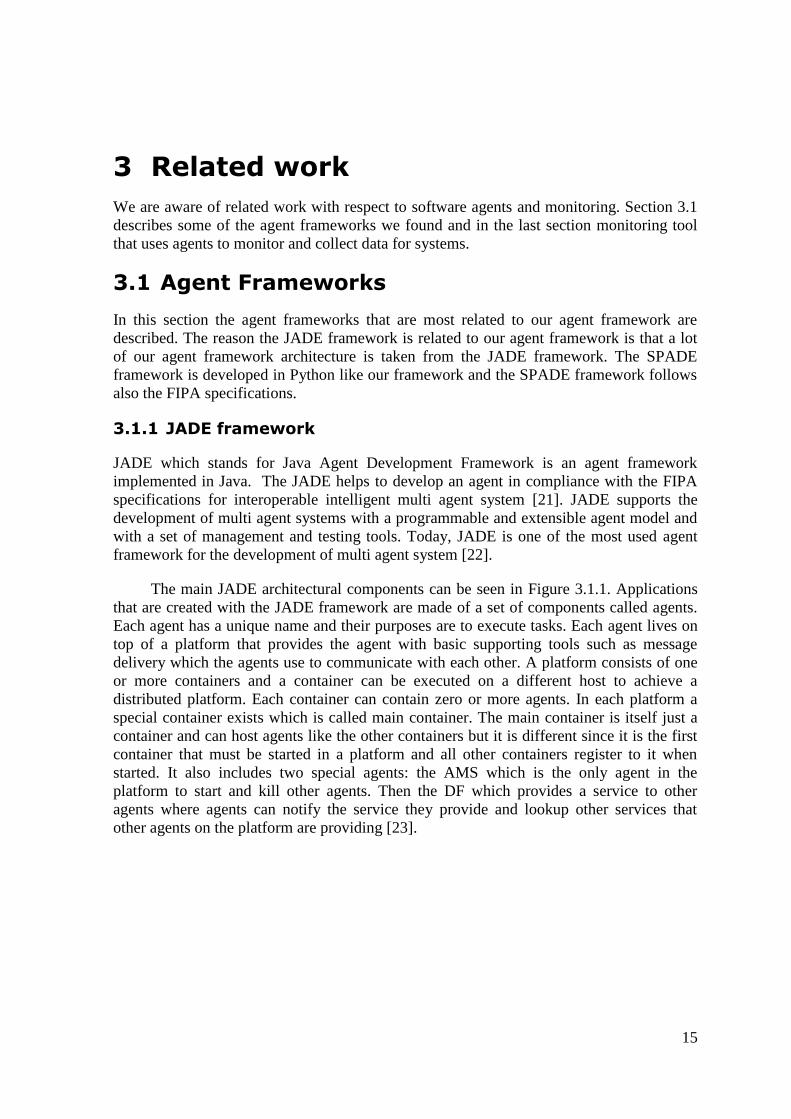


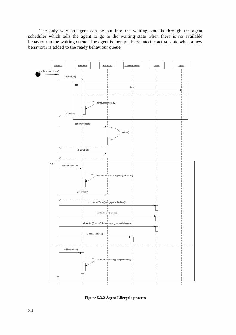


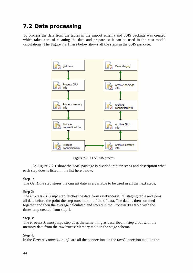


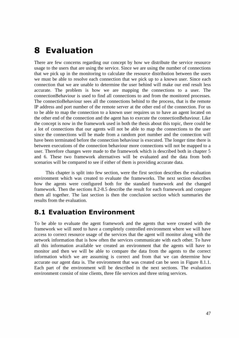


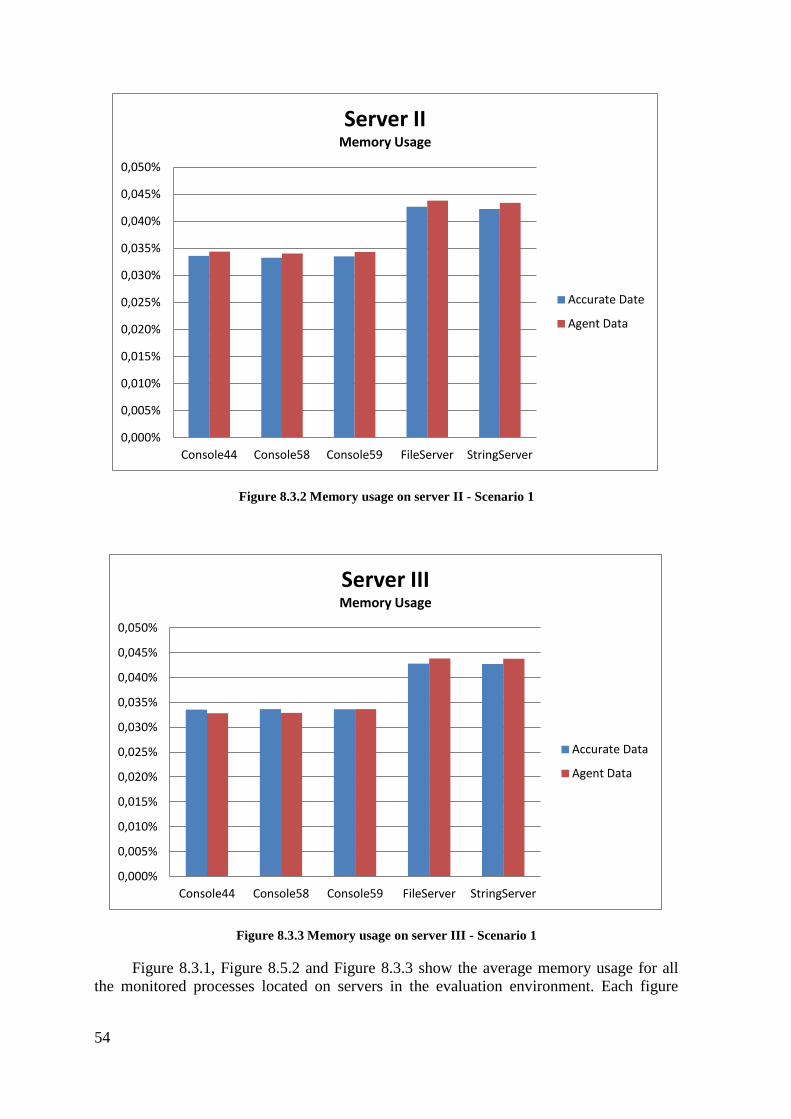
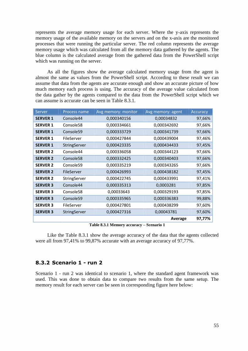


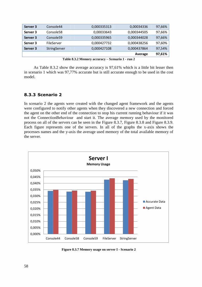


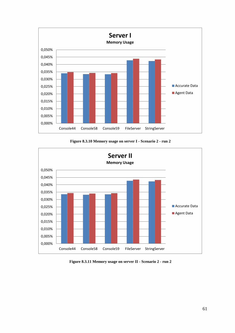


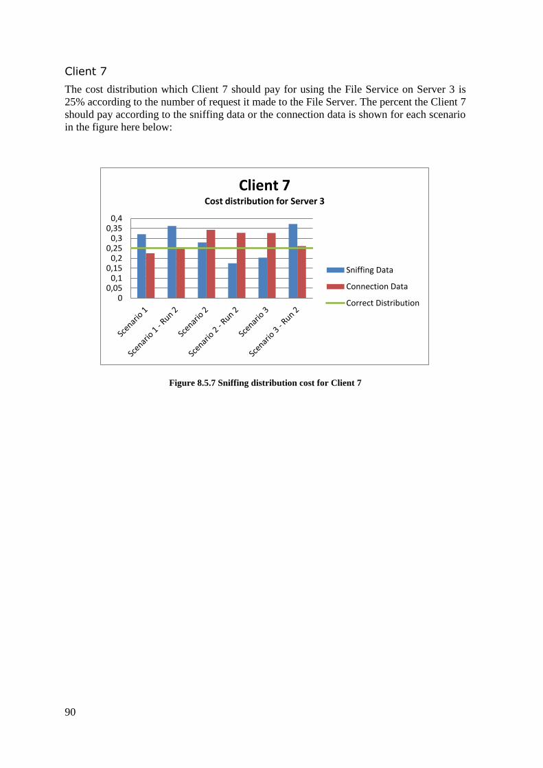


![Best Practices for Oracle Monitoring with Oracle Extended Agent. - IBM · PDF fileBest Practices for Oracle Monitoring with Oracle Extended Agent. Document version [0.3] [Byline for](https://static.documents.pub/doc/80x56/5a705d237f8b9ac0538bea20/best-practices-for-oracle-monitoring-with-oracle-extended-agent-ibm-pdf.jpg)


