Design Demonstration and Optimization of a Morphing

Aircraft Control Surface Using Flexible Matrix Composite Actuators

Edward Brady Doepke

Dissertation proposal submitted to the faculty of the

Virginia Polytechnic Institute and State University

in partial fulfillment of the requirements for the degree of

Doctor of Philosophy

in

Aerospace Engineering

Michael K. Philen, Chair

Robert A. Canfield

Mayuresh J. Patil

Robert L. West

February 16, 2018

Blacksburg, Virginia

Keywords: Morphing, Aircraft Control Surfaces, Flexible Matrix Composite Actuator

Design, Demonstration, and Optimization of a Morphing Aircraft Control Surface

E. Brady Doepke

Abstract

The morphing of aircraft wings for flight control started as a necessity for the Wright Brothers but

quickly fell out of favor as aircraft increased speed. Currently morphing aircraft control is one of

many ideas being explored as we seek to improve aircraft efficiency, reduce noise, and other

alternative aircraft solutions. The conventional hinged control surface took over as the predominant

method for control due to its simplicity and allowing stiffer wings to be built. With modern

technologies in variable stiffness materials, actuators, and design methods, a morphing control

surface, which considers deforming a significant portion of the wing’s surface continuously, can be

considered.

While many have considered morphing designs on the scale of small and medium size UAVs, few

look at it for full-size commercial transport aircraft. One promising technology in this field is the

flexible matrix composite (FMC) actuator. This muscle-like actuator can be embedded with the

deformable structure and unlike many other actuators continue to actuate with the morphing of the

structure. This was demonstrated in the FMC active spoiler prototype, which was a full-scale

benchtop prototype, demonstrated to perform under closed-loop control for both the required

deflection and load cases.

Based on this FMC active spoiler concept a morphing aileron design was examined. To do this an

analysis coupling the structure, fluid, and FMC actuator models was created. This allows for

optimization of the design with the objectives of minimizing the hydraulic energy required and mass

of the system by varying the layout of the FMC aileron, the material properties used, and the

actuator’s design and placement with the morphing section.

Based on a commercial transport aircraft a design case was developed to investigate the optimal

design of a morphing aileron using the developed analysis tool. The optimization looked at

minimizing the mass and energy requirements of the morphing aileron and was subject to a series of

constraints developed from the design case and the physical limitations of the system. A Pareto front

was developed for these two objectives and the resulting designs along the Pareto front explored.

From this optimization, a series of design guidelines were developed.

Design, Demonstration, and Optimization of a Morphing Aircraft Control Surface

E. Brady Doepke

General Audience Abstract

This work looks at an aircraft morphing control surface design on the scale of commercial

transport aircraft. A design is developed and demonstrated through bench top prototype testing and

through analysis. The morphing control surface uses flexible matrix composite (FMC) actuators.

These unique actuators are muscle like, using hydraulic pressure to create a contractive actuator.

Unlike a simple hydraulic piston, the FMC actuators are capable of bending with the morphing

structure during actuation. Through optimization of the morphing control surface design a set of

design guidelines were developed to guide future design.

iv

Acknowledgments

I am very appreciative of the professors whom I have had in class and the AOE department

as a whole. I would particularly like to thank those on my committee, Dr. Canfield, Dr. Patil,

Dr. Philen, and Dr. West. I would like to thank Dr. West for his initial insight into setting up

parametric models in Abaqus, and Dr. Canfield for his course in structural optimization. I

would especially like to thank Dr. Philen. He has created a lab and environment that is fun to

work in and has offered many exciting challenges and projects along the way. Unfortunately,

many of these side projects did not make it into this dissertation. He has provided guidance

when needed and great freedom along the way. I will miss his flying (crashing) of quads, Jeep,

rides, annual BBQ, and much more.

I would like to thank everyone who has been down in the ASML and passed through over

the years. There are too many to name, but I learned something working with each. I would

like to especially thank Shawn and Carson, both were there to see me through the end. Shawn

too will soon be done, but Carson’s time continues, and I expect he will accomplish great

things. I have particularly enjoyed my time with Carson who has been one of the best people

to work with. His help has likely sped me up equally as much as his friendship and antics has

slowed me down.

I would also like the thank everyone at my new home, NASA MSFC. Getting the

opportunity to seamlessly take the next step after my Ph.D., and to contribute to meaningful

work has been a great inspiration at the end. They have been gracious working with and

encouraging me to finish.

The last few years I have had the opportunity to be an instructor in the ENGE department

and would like to thank the many students I have had and the ENGE department who not

only funded me but provided guidance during one of the best parts of my time at Tech. I

enjoyed teaching and learned a great deal. I would like to thank Dr. Butler and Dr. Reid, who

v

likely do not realize, through their example alone taught me a great deal. I would especially

like to thank Dr. Butler for always providing a practicing engineer’s perspective on matters.

My wife, Leah, deserves much of the credit. She took the dive with me and supported me

throughout. Without her I likely would not have made it through that first semester.

To my family: my brothers, sister, nieces, and nephews have all served as inspiration along

the way whether they were aware or not. This includes my wife’s family, particularly her

parents, who have been a great help along the way.

Finally, and most importantly I owe thanks to my parents, who from the youngest age

supported me. I truly grew up in a home where I could build, take apart, try, and do most

anything a future engineer would want.

vi

Table of Contents

Abstract .......................................................................................................................................... ii

General Audience Abstract ......................................................................................................... iii

Acknowledgments ........................................................................................................................ iv

1 Introduction and Literature Review .................................................................................... 1

1.1 Morphing Aircraft Concepts ............................................................................................ 2

1.1.1 The Origins of Morphing .......................................................................................... 3

1.1.2 VCCTEF ................................................................................................................... 6

1.1.3 Piezoelectric Actuated Morphing Designs ................................................................ 8

1.1.4 UAV Flight Control With Twisting Acutation ....................................................... 10

1.1.5 FishBAC ................................................................................................................. 12

1.1.6 FlexSys .................................................................................................................... 13

1.2 Fluid Driven Actuators ................................................................................................... 14

1.3 Motivation and Dissertation Outline .............................................................................. 20

2 Design and Testing of a Morphing FMC Spoiler .............................................................. 22

2.1 Model-Based Design ...................................................................................................... 23

2.2 FMC Actuator Fabrication ............................................................................................. 26

2.3 Active Spoiler Prototype ................................................................................................ 28

2.3.1 Design and Fabrication ........................................................................................... 28

2.3.2 Quasistatic Experiments.......................................................................................... 29

2.3.3 Dynamic Testing of the Active Spoiler and FE Validation .................................... 31

2.3.4 System identification and closed-loop results for the active spoiler ....................... 33

2.4 Active spoiler conclusions ............................................................................................. 38

3 Model Development for the Morphing FMC Aileron ...................................................... 40

3.1 Design Case Definition and Design Variables ............................................................... 40

3.2 Characterization of FMC actuators ................................................................................ 45

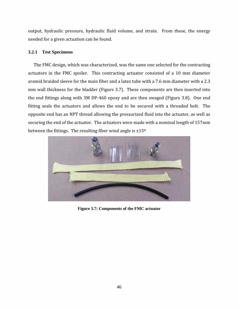
3.2.1 Test Specimens ....................................................................................................... 46

3.2.2 Fluid Volume Characterization ............................................................................... 47

3.2.3 Force, Displacement, and Pressure Characterization .............................................. 48

3.2.4 Actuator Passive Stiffness....................................................................................... 51

3.2.5 Empirical Model ..................................................................................................... 52

3.3 Coupled Structural and Fluid Solution ........................................................................... 56

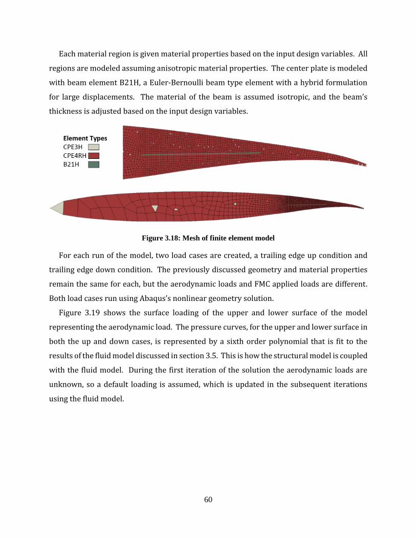
3.4 Structural Solution.......................................................................................................... 59

vii

3.4.1 Structural Model of FMC actuator .......................................................................... 61

3.5 XFOIL Fluid Solution .................................................................................................... 63

3.6 Conclusion ...................................................................................................................... 65

4 Parameter Study for the Morphing FMC Aileron ........................................................... 67

4.1 Observed Trends ............................................................................................................ 67

4.2 Baseline Solution............................................................................................................ 68

4.3 Flap Deflection ............................................................................................................... 71

4.4 Hinge Line Location and Active Length ........................................................................ 75

4.5 FMC Installed Bias......................................................................................................... 79

4.6 Position of Internal Components .................................................................................... 81

4.7 Polymer Stiffness and Center Plate Thickness ............................................................... 87

4.8 Conclusion ...................................................................................................................... 89

5 Optimization......................................................................................................................... 90

5.1 Objective Function ......................................................................................................... 90

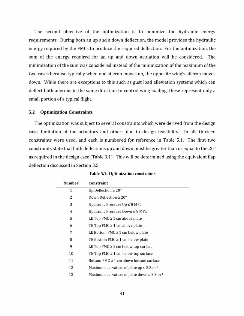
5.2 Optimization Constraints................................................................................................ 91

5.3 Optimization Method ..................................................................................................... 93

5.4 Optimization Results ...................................................................................................... 96

5.4.1 Hinge Line and Active Length ................................................................................ 97

5.4.2 Internal Layout of FMCs and Plate ......................................................................... 98

5.4.3 Convergence Limits of the Analysis ..................................................................... 101

5.4.4 Passive Stiffness Design Variables ....................................................................... 103

5.4.5 Strain and Energy of the FMC Actuators ............................................................. 105

5.5 Design Point Comparison and Conclusions ................................................................. 109

6 Conclusions and Recommendations................................................................................. 115

6.1 Conclusions .................................................................................................................. 115

6.2 Future Work ................................................................................................................. 116

Appendix A ................................................................................................................................ 119

References .................................................................................................................................. 129

viii

List of Figures

Figure 1.1: Picture of the 1903 Wright Flyer's Maiden Flight December 17th, 1903, Kitty Hawk

NC [18] ........................................................................................................................................... 3

Figure 1.2: Top) 1903 Wright Flyer with warped wings [18] Bottom) Drawings from the Wright

Brother's first patent on wing warping [19]. ................................................................................... 4

Figure 1.3: Clement Ader’s Eole concept from 1890 [21] ............................................................. 5

Figure 1.4: Left) The WhoopingMAV with varying gull wing positions Right) Seagull with

wings positioned for soaring and diving [24] ................................................................................. 5

Figure 1.5: Left) NextGen MFX-1 UAV showing the two extremes of planform change[25],

Right) A peregrine falcon going from soaring to a steep dive in an action called a stoop ............. 6

Figure 1.6: A) three-part flap of the VCCTEF. B) Continuous trailing edge flap of the VCCTEF

with exaggerated deflections. [29] .................................................................................................. 7

Figure 1.7: A) Optimized flap position for the VCCTEF at four different flight conditions. B)

Pressure distribution on the top surface for the GTM and optimized VCCTEF at midcruise [29]. 7

Figure 1.8: MFC control surfaces on the main wing and tail [30]. ................................................. 8

Figure 1.9: Morphing aircraft with MFC actuators in flight [30] ................................................... 8

Figure 1.10: The SMTE concept using alternating sections of MFC controlled morphing and

passive transition sections. [32] ...................................................................................................... 9

Figure 1.11: Approaches to morphing for flight control: camber change (left), local camber

change (center), and angle of attack or twist (right) [34]. ............................................................ 10

Figure 1.12: Internal structure of morphing control surface (left) and the complete control surface

with lower access panel removed (right) [33]............................................................................... 11

Figure 1.13: UAV with wing warping tips during ground deflection and maiden flight [33]. ..... 11

Figure 1.14: LE and TE view of the left morphing surface during a right roll maneuver [33]. ... 12

Figure 1.15: A) FishBAC prototype and B) FishBAC concept [36]. ........................................... 12

Figure 1.16: Pareto plots of optimal solutions for the FishBAC concept for the objective of mass,

drag, and actuation energy. ........................................................................................................... 13

Figure 1.17: FlexSys Inc. flexible trailing edge fitted to NASA’s G III aircraft for flight testing as

part of the ACTE program [42]. ................................................................................................... 14

Figure 1.18: Cross-section of a typical aircraft control surface area showing hydraulic cylinder

(16) [48] ........................................................................................................................................ 15

Figure 1.19: A) Wet filament winding process B) Effect of fiber wind angle on actuation. ........ 16

Figure 1.20: Stiffness modulation vs. lower modulus for FMC actuators and several other

variable modulus materials [54] .................................................................................................... 17

Figure 1.21: Left) The KAFO prosthetic use PAM actuators [55]. Right) FESTO’s humanoid

robot using PAM actuators and close up detail of the shoulder joint [56]. .................................. 18

ix

Figure 1.22: The completed FMC morphing flap at 0 and 7 cm deflection (left). Single FMC in

parallel runs before casting (right) [57] ........................................................................................ 19

Figure 1.23: eSPAARO FMC flap with 7 cm deflection and the ground track of the test flight

[57] ................................................................................................................................................ 19

Figure 2.1: Morphing Spoiler Concept ......................................................................................... 23

Figure 2.2: Partitioned and meshed FE model .............................................................................. 24

Figure 2.3: A) Boundary conditions and loads for blocked case. B) First design iteration

showing undesired deflection ....................................................................................................... 24

Figure 2.4: (A) Model with composite centerline plate. (B) Polymer and honeycomb composite

....................................................................................................................................................... 25

Figure 2.5: FE modal analysis results for the first two natural frequencies ................................. 26

Figure 2.6: (A) Example FMC actuators – actuators are fabricated using wet-filament winding

process, and dry braided sleeves later cast in a polymer resin and (B) Typical force and strain

results for an actuator at constant pressure and in a blocked condition. ....................................... 27

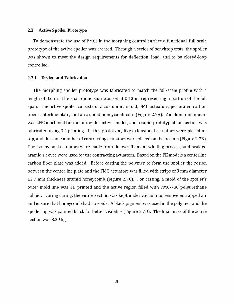
Figure 2.7: (A) Designed spoiler prototype, (B) assembled spoiler before casting without

honeycomb core (C) active spoiler with honeycomb core before casting and (D) active spoiler

after casting in PMC 780 polyurethane ........................................................................................ 29

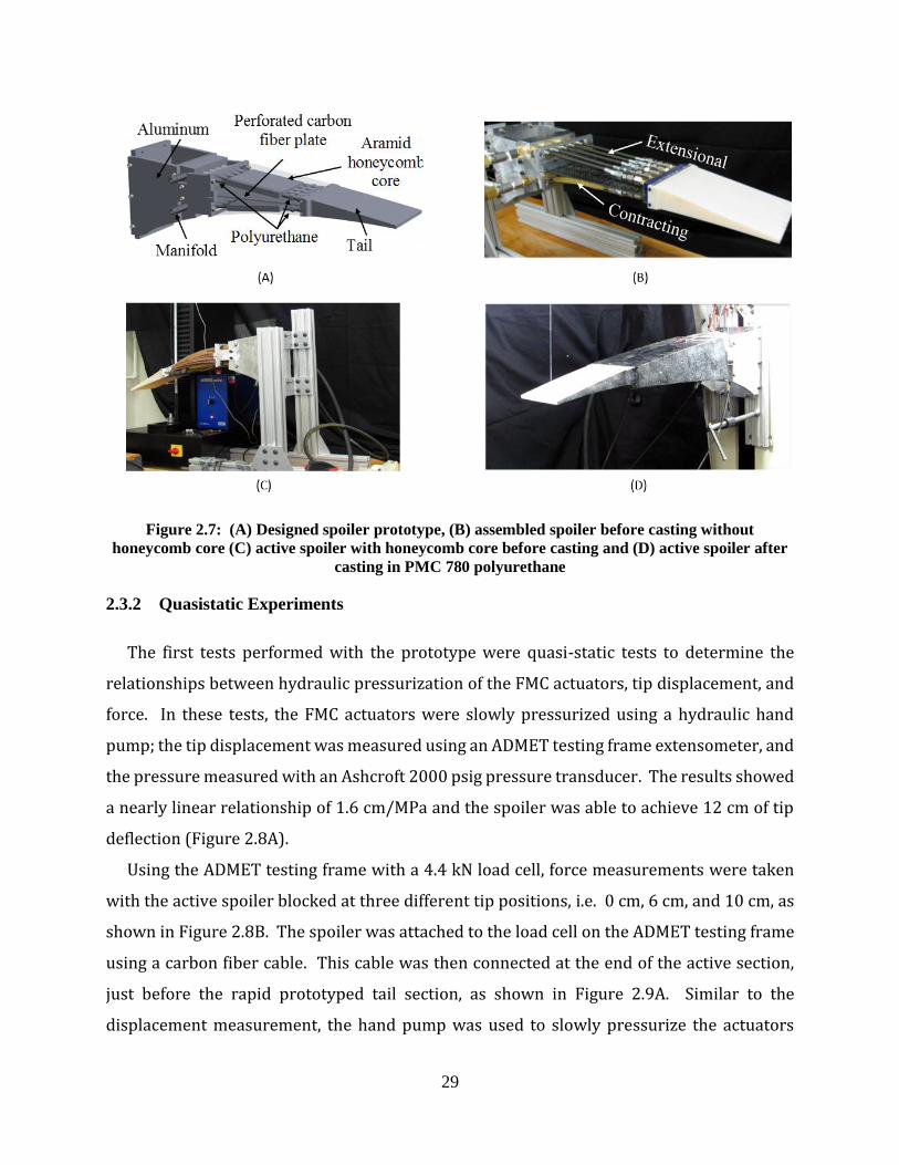
Figure 2.8: (A) Tip free displacement with increased actuation pressure and (B) measured force

of the spoiler at different constrained tip displacements .............................................................. 30

Figure 2.9: (A) Force measurement testing setup and (B) unpressurized stiffness result ............ 31

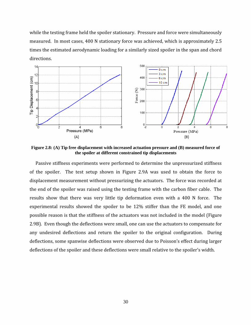
Figure 2.10. Experiment setup for dynamic system analysis....................................................... 32

Figure 2.11: (A) Frequency response of tip velocity to the applied force for different initial

pressures. With an increase in pressure, the first resonant frequency is increasing. (B)

Frequency response of internal pressure to the applied force for different initial pressures. ....... 33

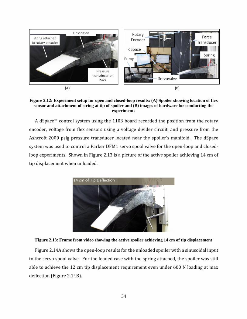
Figure 2.12: Experiment setup for open and closed-loop results: (A) Spoiler showing location of

flex sensor and attachment of string at tip of spoiler and (B) images of hardware for conducting

the experiments ............................................................................................................................. 34

Figure 2.13: Frame from video showing the active spoiler achieving 14 cm of tip displacement 34

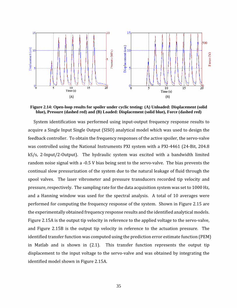
Figure 2.14: Open-loop results for spoiler under cyclic testing: (A) Unloaded: Displacement

(solid blue), Pressure (dashed red) and (B) Loaded: Displacement (solid blue), Force (dashed

red) ................................................................................................................................................ 35

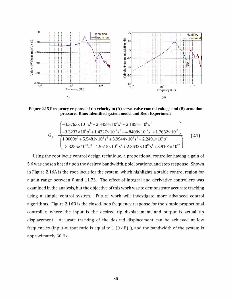
Figure 2.15 Frequency response of tip velocity to (A) servo-valve control voltage and (B)

actuation pressure. Blue: Identified system model and Red: Experiment ................................... 36

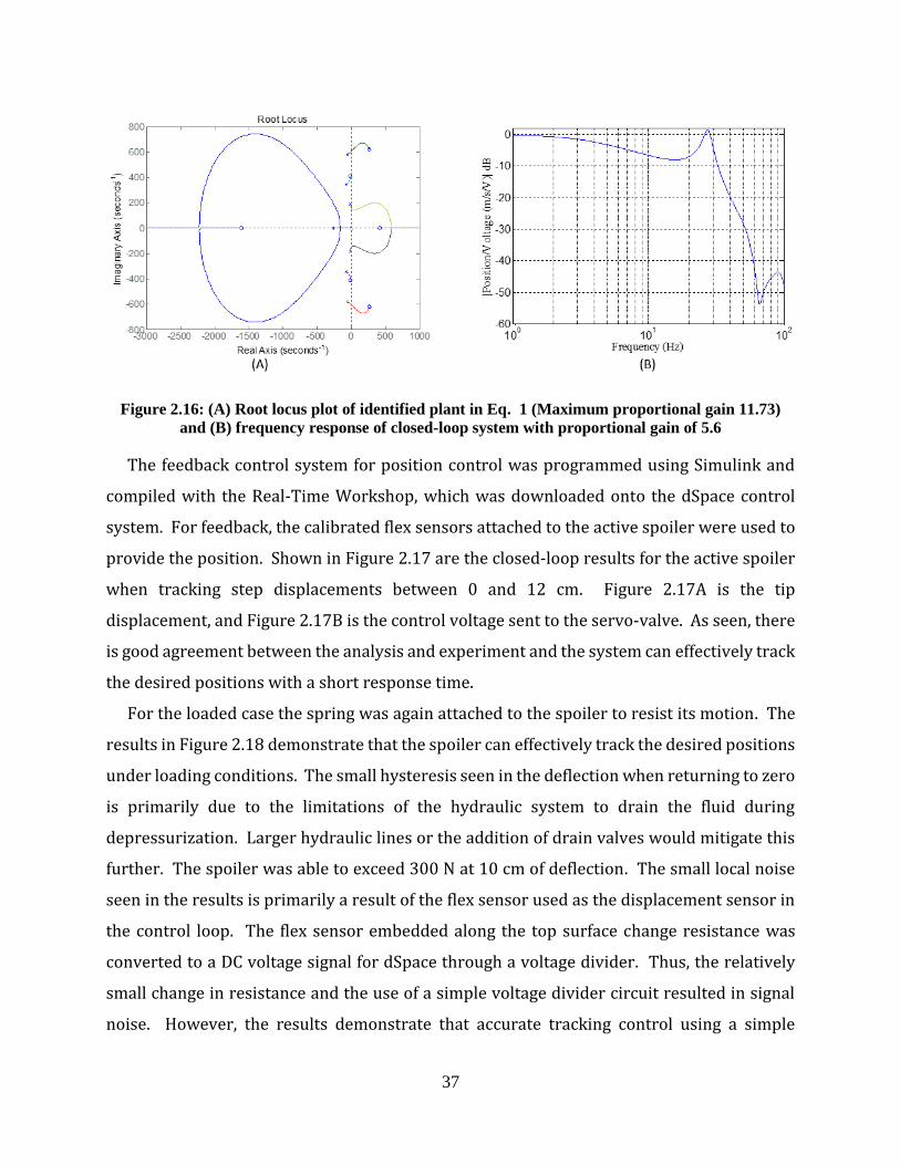
Figure 2.16: (A) Root locus plot of identified plant in Eq. 1 (Maximum proportional gain 11.73)

and (B) frequency response of closed-loop system with proportional gain of 5.6 ....................... 37

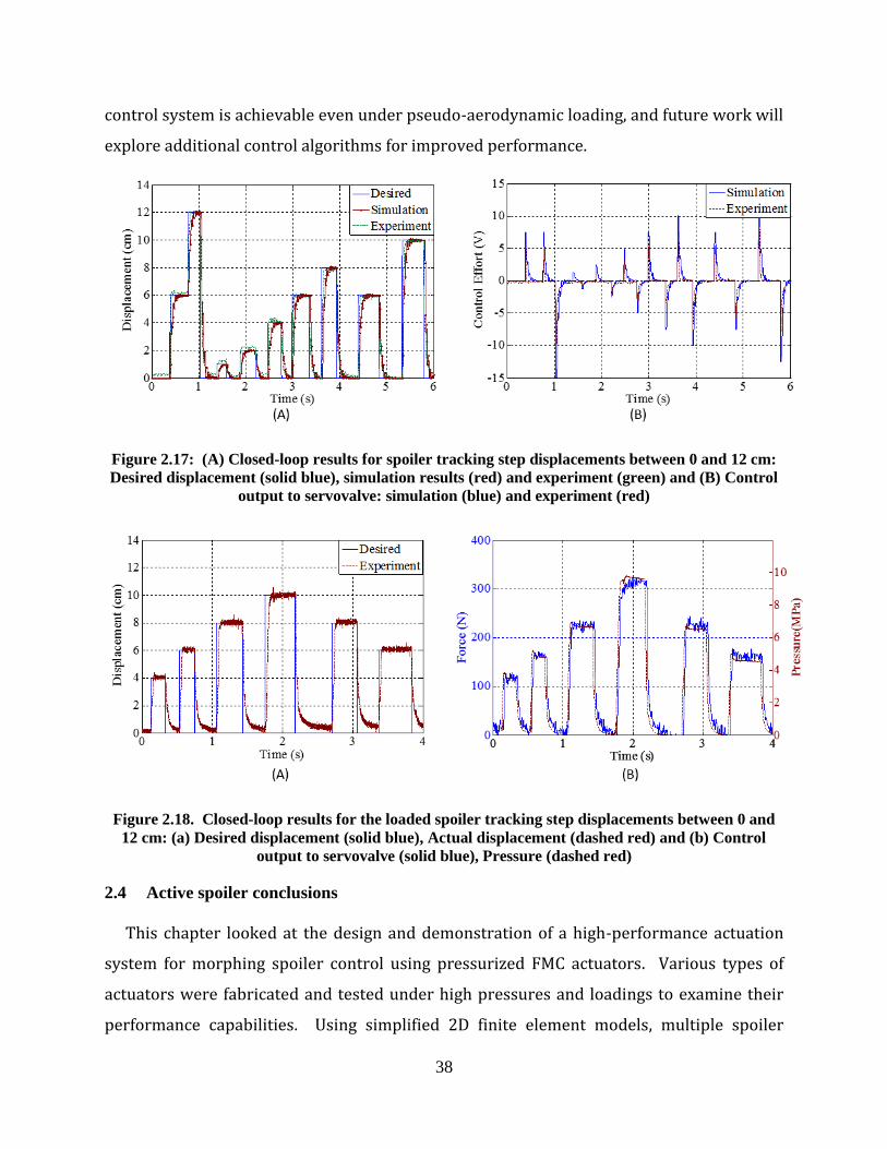
Figure 2.17: (A) Closed-loop results for spoiler tracking step displacements between 0 and 12

cm: Desired displacement (solid blue), simulation results (red) and experiment (green) and (B)

Control output to servovalve: simulation (blue) and experiment (red)......................................... 38

x

Figure 2.18. Closed-loop results for the loaded spoiler tracking step displacements between 0

and 12 cm: (a) Desired displacement (solid blue), Actual displacement (dashed red) and (b)

Control output to servovalve (solid blue), Pressure (dashed red) ................................................. 38

Figure 3.1: A) Computational and wind tunnel models of the NASA CRM aircraft [64] [65]. ... 41

Figure 3.2: Airfoil profile of the outboard section of the NASA CRM main wing. ..................... 41

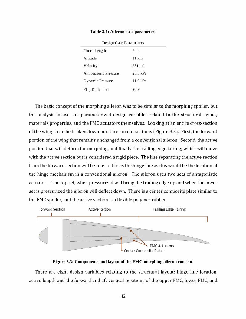
Figure 3.3: Components and layout of the FMC morphing aileron concept. ............................... 42

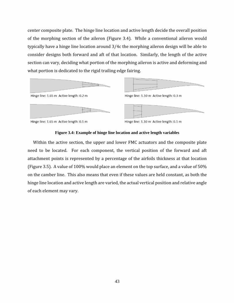
Figure 3.4: Example of hinge line location and active length variables ....................................... 43

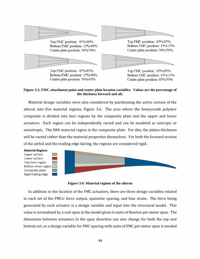
Figure 3.5: FMC attachment point and center plate location variables. Values are the percentage

of the thickness forward and aft. ................................................................................................... 44

Figure 3.6: Material regions of the aileron ................................................................................... 44

Figure 3.7: Components of the FMC actuator .............................................................................. 46

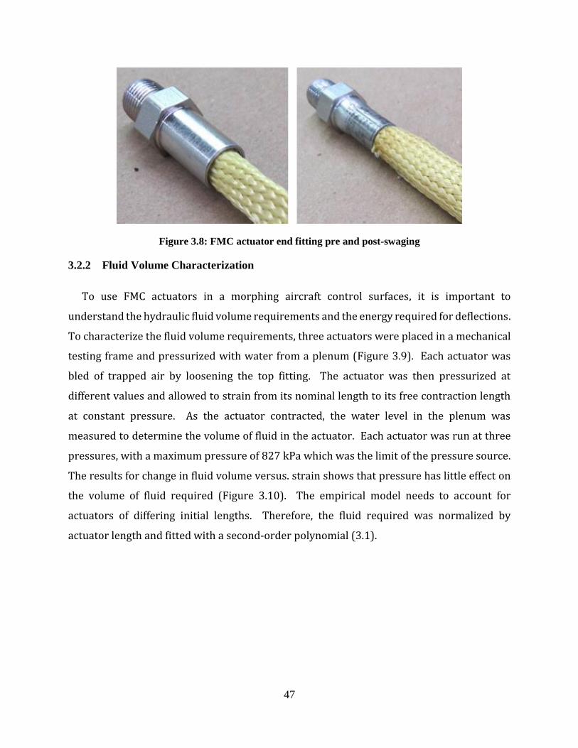
Figure 3.8: FMC actuator end fitting pre and post-swaging ......................................................... 47

Figure 3.9: Fluid volume test setup............................................................................................... 48

Figure 3.10: Change in FMC fluid volume vs. strain and pressure for a 157 mm length actuator48

Figure 3.11: Test setup for force, displacement, and pressure characterization. .......................... 49

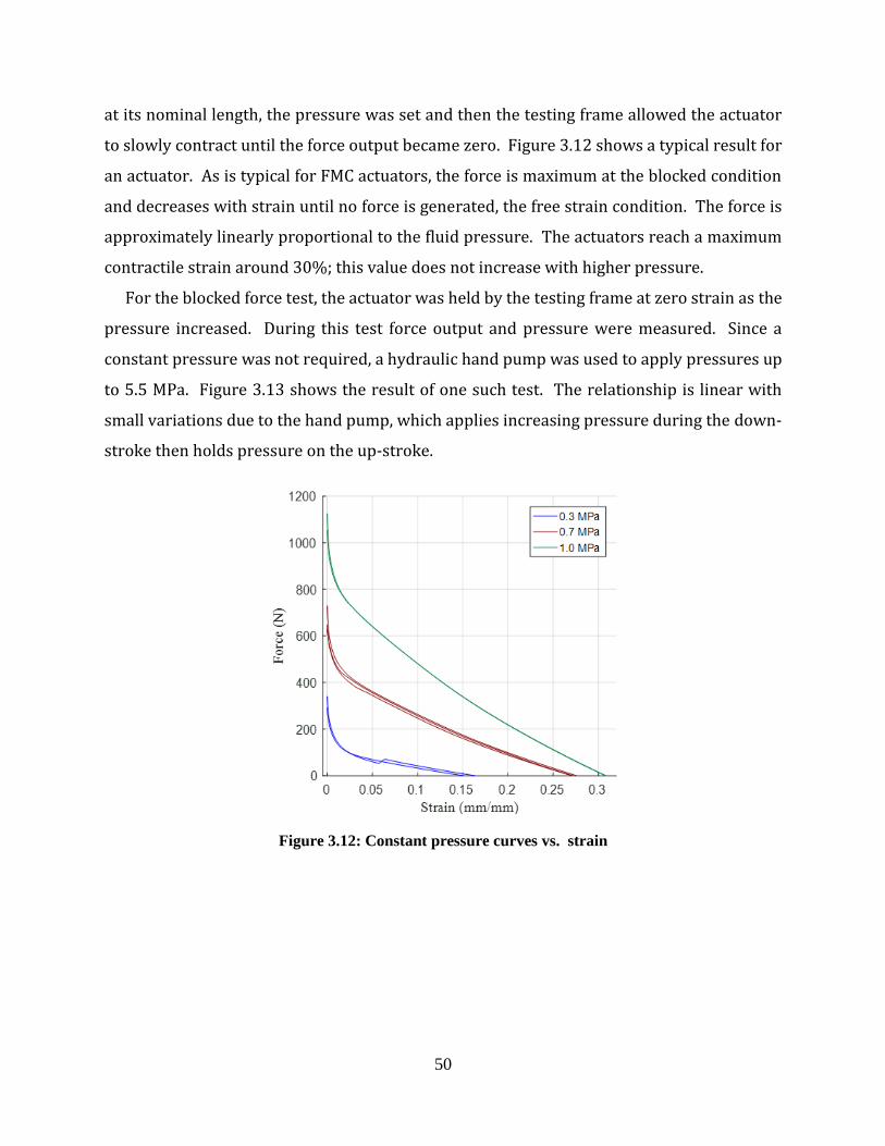
Figure 3.12: Constant pressure curves vs. strain.......................................................................... 50

Figure 3.13: Result of a typically blocked force test .................................................................... 51

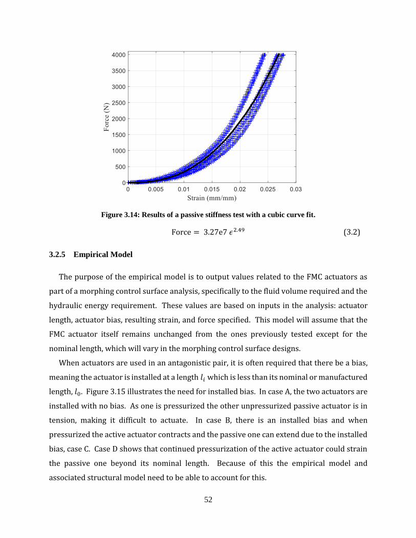
Figure 3.14: Results of a passive stiffness test with a cubic curve fit. ......................................... 52

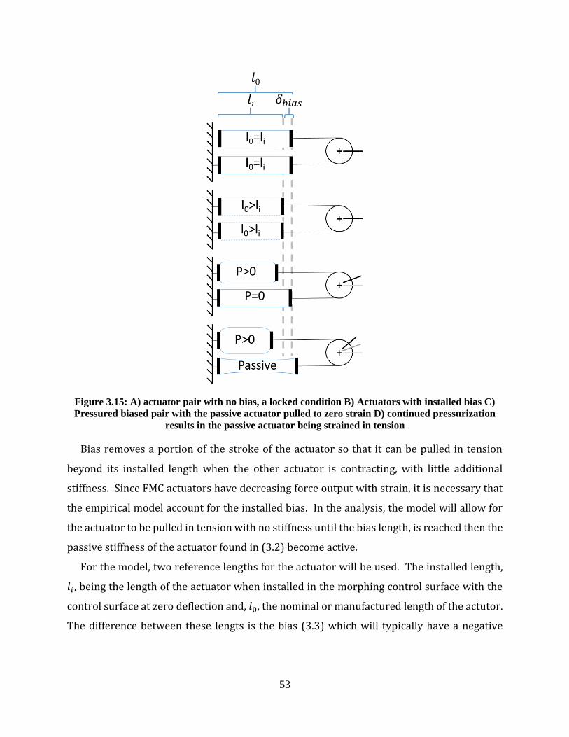
Figure 3.15: A) actuator pair with no bias, a locked condition B) Actuators with installed bias C)

Pressured biased pair with the passive actuator pulled to zero strain D) continued pressurization

results in the passive actuator being strained in tension ............................................................... 53

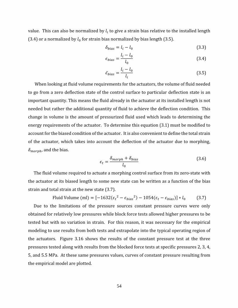
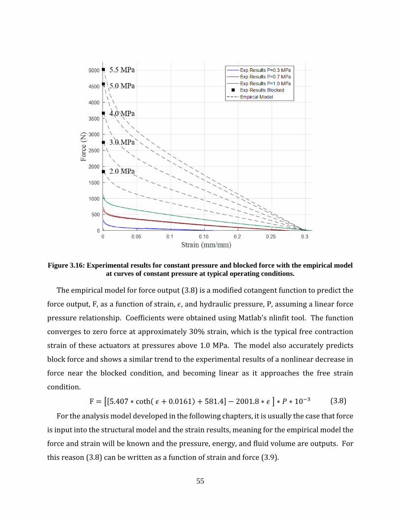
Figure 3.16: Experimental results for constant pressure and blocked force with the empirical

model at curves of constant pressure at typical operating conditions. .......................................... 55

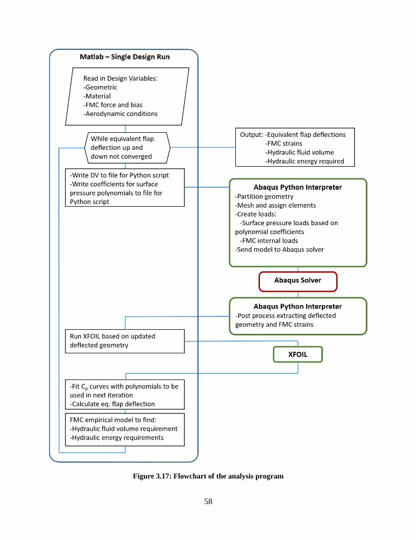
Figure 3.17: Flowchart of the analysis program ........................................................................... 58

Figure 3.18: Mesh of finite element model ................................................................................... 60

Figure 3.19: Model with applied surface loads for aerodynamics ................................................ 61

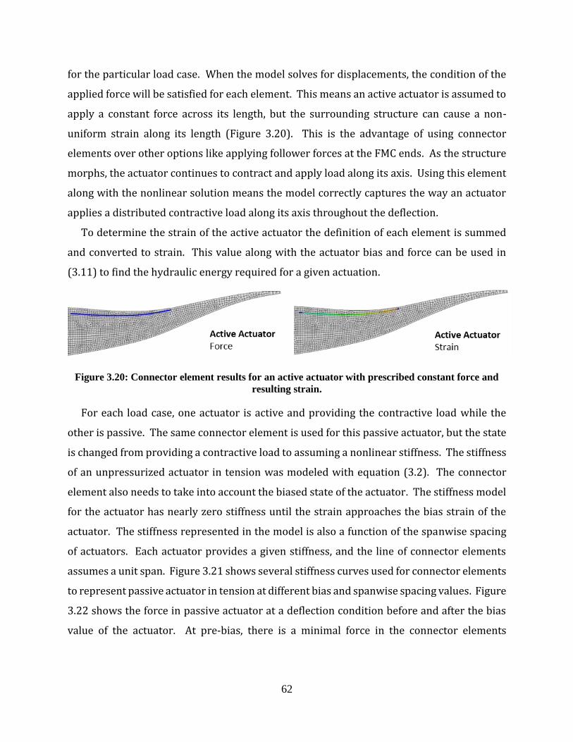
Figure 3.20: Connector element results for an active actuator with prescribed constant force and

resulting strain. .............................................................................................................................. 62

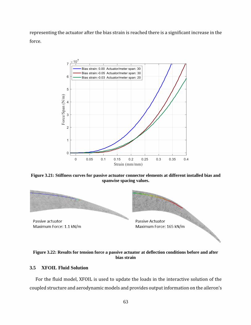
Figure 3.21: Stiffness curves for passive actuator connector elements at different installed bias

and spanwise spacing values. ........................................................................................................ 63

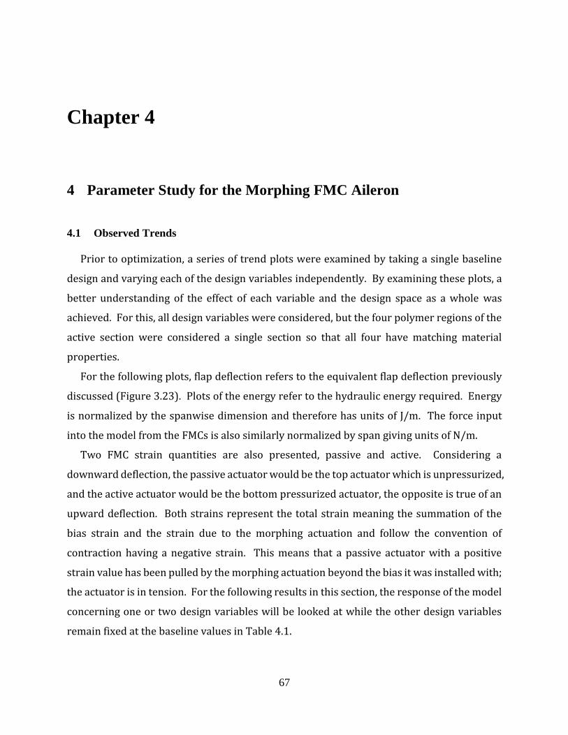
Figure 3.22: Results for tension force a passive actuator at deflection conditions before and after

bias strain ...................................................................................................................................... 63

Figure 3.23: Geometry for the CRM airfoil with conventional aileron and results of XFOIL

analysis for equivalent flap deflection. ......................................................................................... 65

Figure 4.1: ±20° deflection of the baseline case, entire airfoil. .................................................... 70

Figure 4.2: Deflection for ±20° deflection of the baseline case, active region and trailing edge

fairing. ........................................................................................................................................... 70

Figure 4.3: Connector force of the passive and active actuators in the baseline solution with 3%

bias. ............................................................................................................................................... 70

xi

Figure 4.4: Connector force of the passive and active actuators in the baseline solution with 1.5%

bias. ............................................................................................................................................... 71

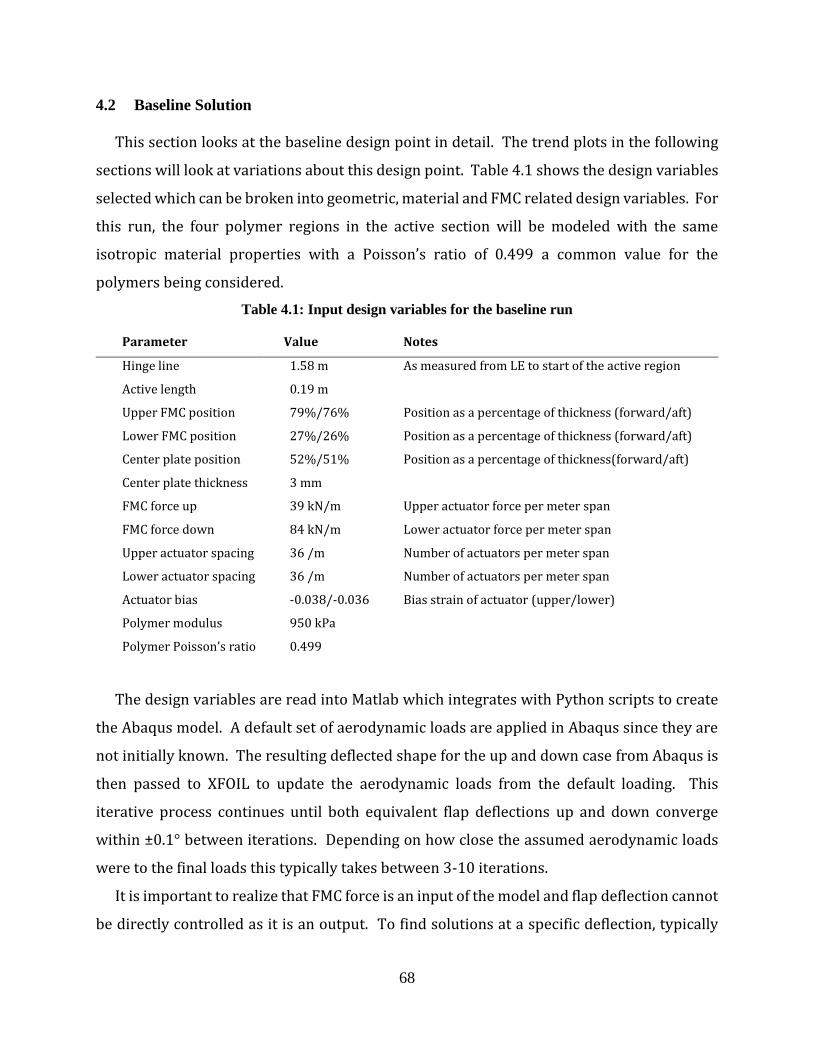
Figure 4.5: Resulting FMC force and hydraulic energy required for deflection from 0-20°. ...... 72

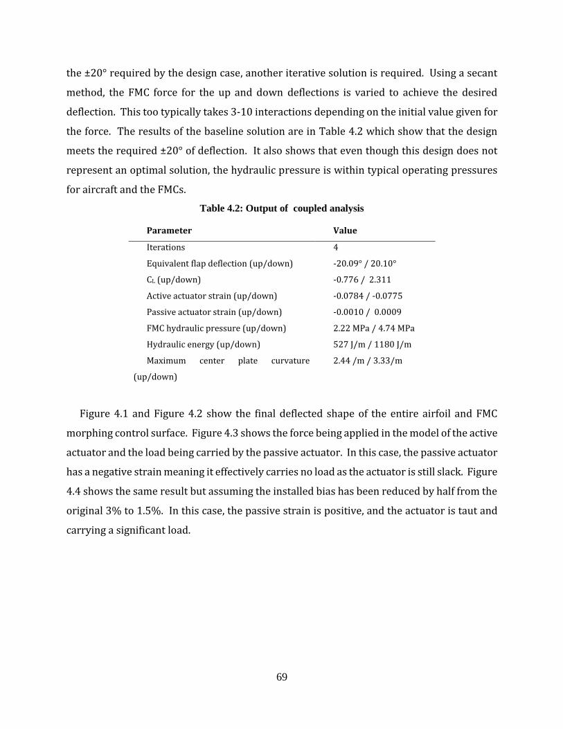
Figure 4.6: Comparing the force and energy required for the default flow case and a case with no

flow ............................................................................................................................................... 73

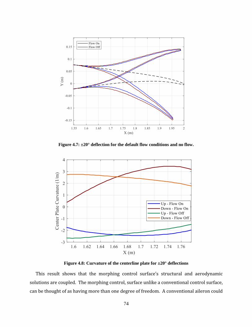
Figure 4.7: ±20° deflection for the default flow conditions and no flow. .................................... 74

Figure 4.8: Curvature of the centerline plate for ±20° deflections ............................................... 74

Figure 4.9: Energy and passive FMC strain for a 12° downward deflection with varying hinge

line location and active length. Circled data markers indicate passive actuator is taut. .............. 76

Figure 4.10: Energy and passive FMC strain for a 12° upward deflection with varying hinge line

location and active length. Circled data markers indicate passive actuator is taut. ..................... 76

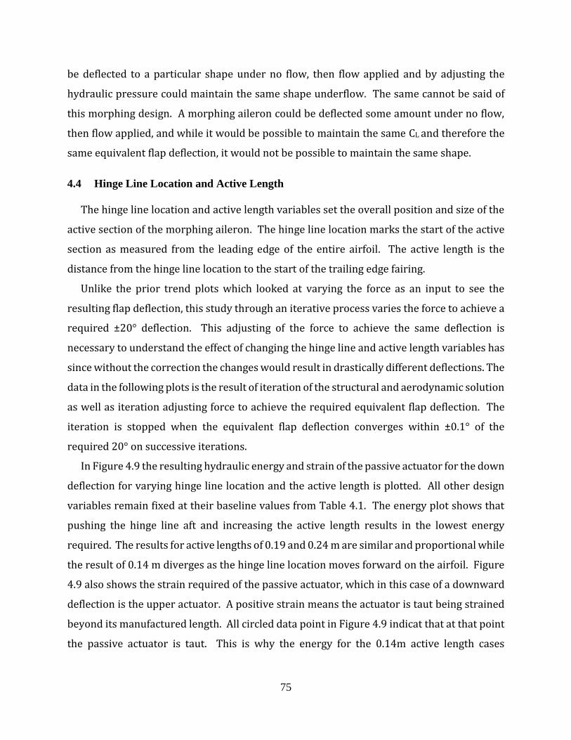
Figure 4.11: Displacement contour for hinge line location of 1.63 m and active length 0.24 m . 77

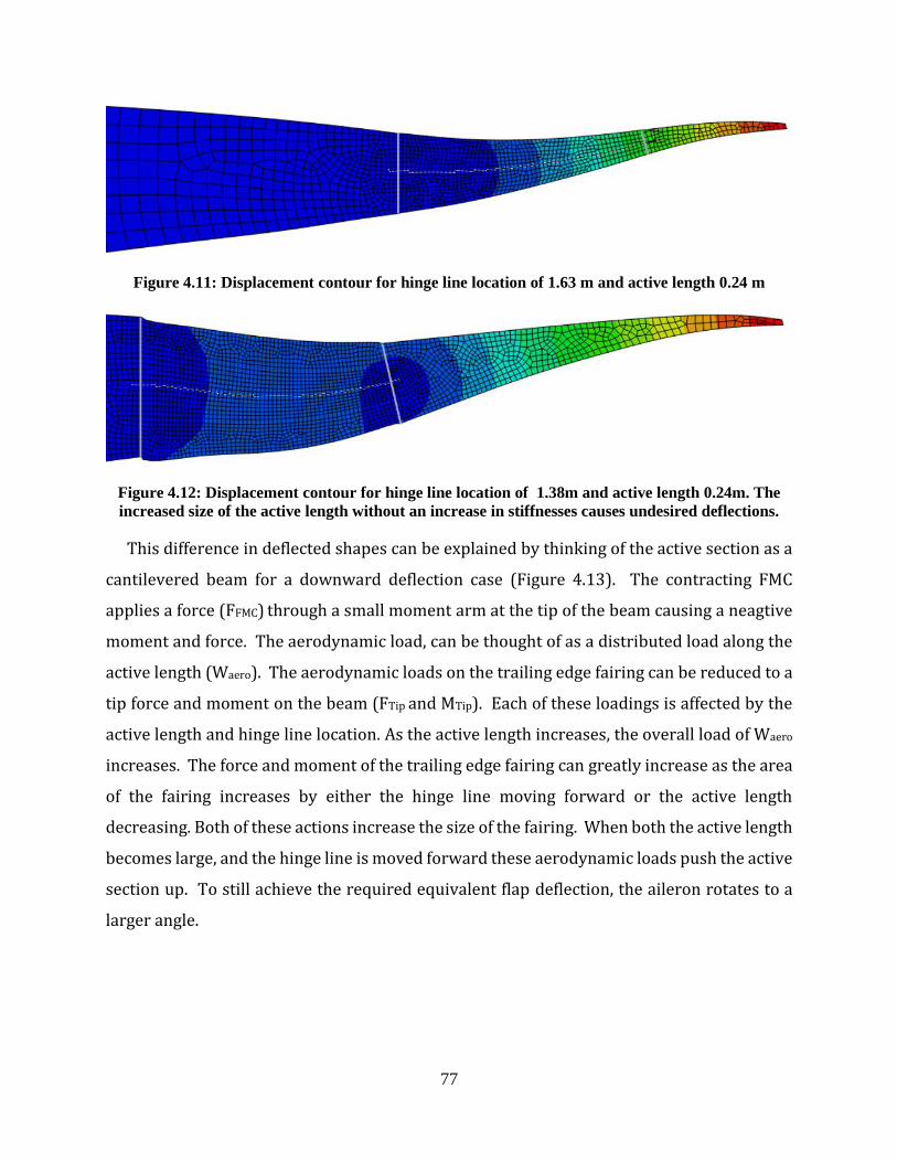
Figure 4.12: Displacement contour for hinge line location of 1.38m and active length 0.24m.

The increased size of the active length without an increase in stiffnesses causes undesired

deflections. .................................................................................................................................... 77

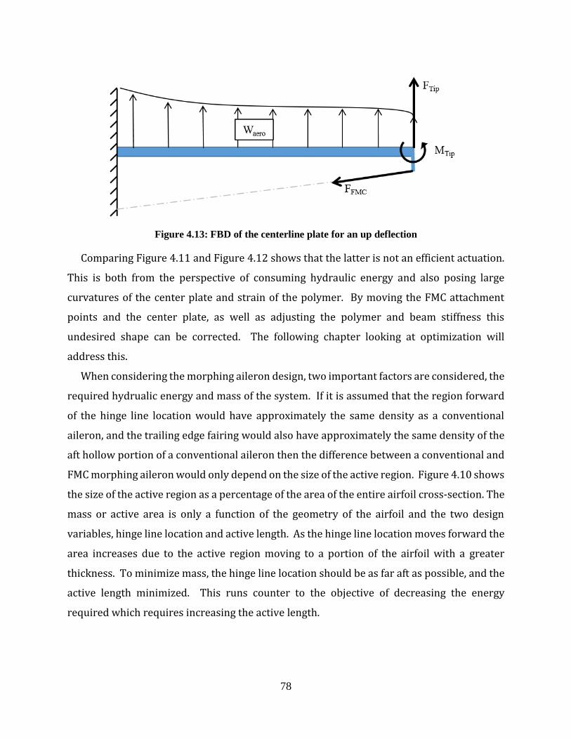
Figure 4.13: FBD of the centerline plate for an up deflection ...................................................... 78

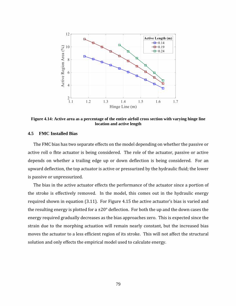
Figure 4.14: Active area as a percentage of the entire airfoil cross section with varying hinge line

location and active length ............................................................................................................. 79

Figure 4.15: Energy for ±20° deflection with varying active FMC bias. ..................................... 80

Figure 4.16: Energy for ±20° deflection with varying passive FMC bias. ................................... 80

Figure 4.17: Deflected shaped for a downward deflection with 1% and 6% bias in the upper

actuator. ......................................................................................................................................... 81

Figure 4.18: the Hydraulic energy required for an upward deflection of 20° with varying forward

and aft location of the centerline plate. ......................................................................................... 82

Figure 4.19: Strain required of the active top actuator set for a 20° deflection with varying plate

location .......................................................................................................................................... 83

Figure 4.20: FMC force required for an upward deflection with varying centerline plate position.

....................................................................................................................................................... 83

Figure 4.21: The total energy required for ±20° deflection with varying forward and aft

attachment points of the centerline plate. ..................................................................................... 84

Figure 4.22: Energy required for a 20° downward deflection with varying bottom FMC location

....................................................................................................................................................... 85

Figure 4.23: Strain for a 20° downward deflection with varying bottom FMC location ............. 85

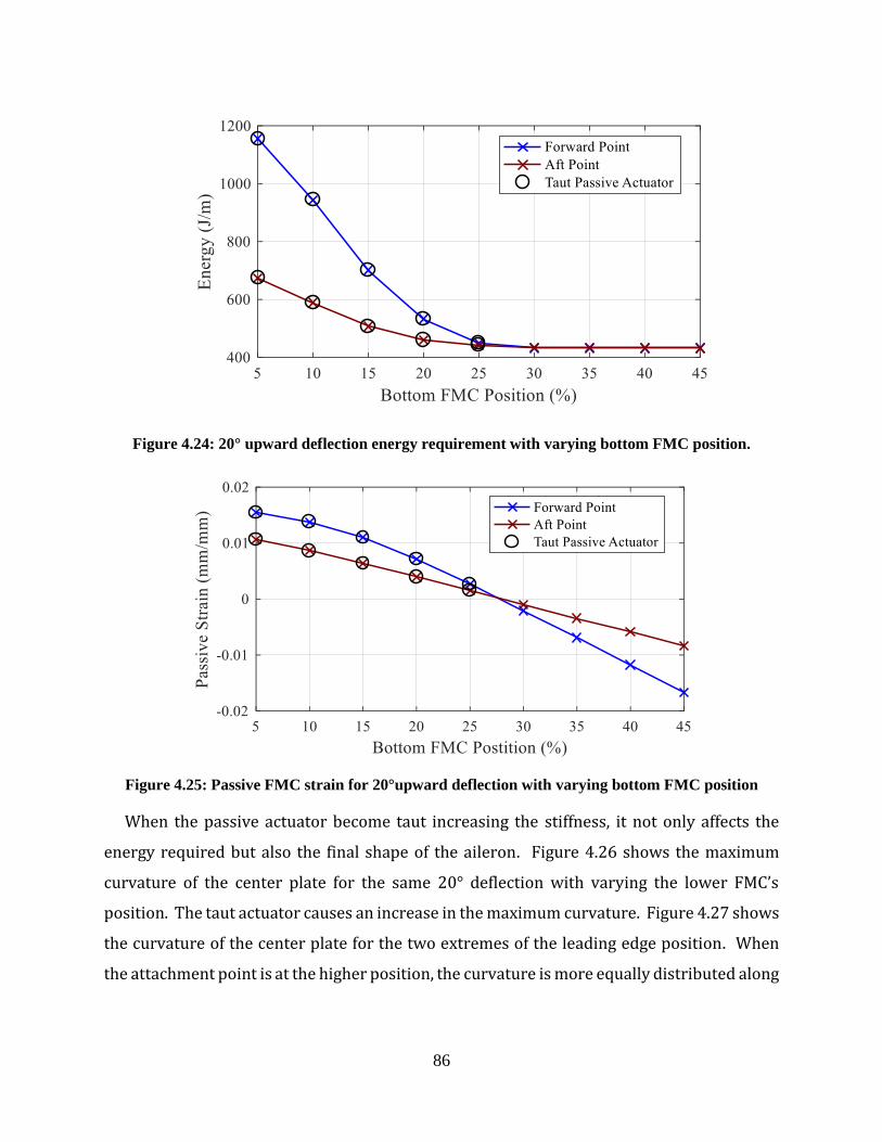
Figure 4.24: 20° upward deflection energy requirement with varying bottom FMC position. .... 86

Figure 4.25: Passive FMC strain for 20°upward deflection with varying bottom FMC position 86

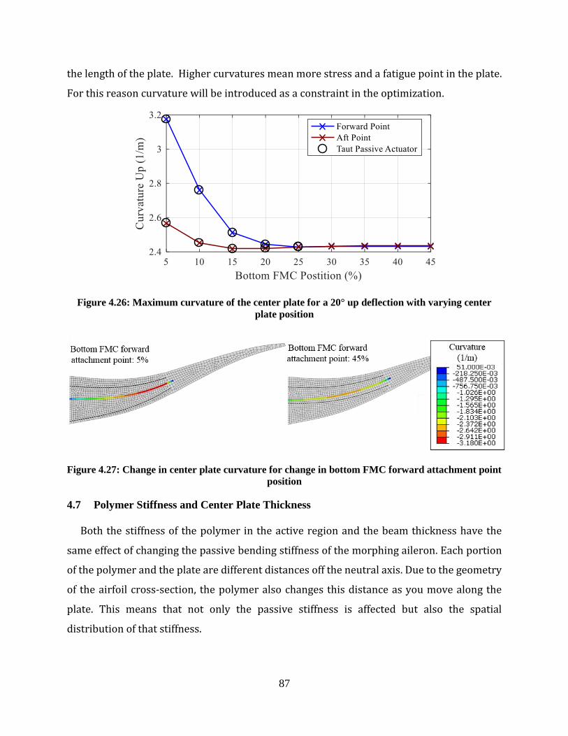
Figure 4.26: Maximum curvature of the center plate for a 20° up deflection with varying center

plate position ................................................................................................................................. 87

Figure 4.27: Change in center plate curvature for change in bottom FMC forward attachment

point position ................................................................................................................................ 87

xii

Figure 4.28: Change in energy required for changing polymer stiffness with all four-polymer

regions set equal. ........................................................................................................................... 88

Figure 4.29: Change in required energy for changing center plate thickness. .............................. 89

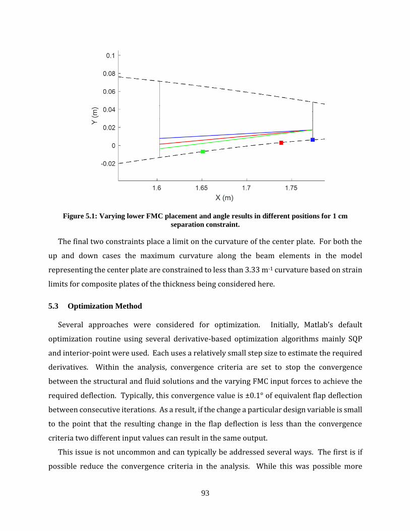
Figure 5.1: Varying lower FMC placement and angle results in different positions for 1 cm

separation constraint. .................................................................................................................... 93

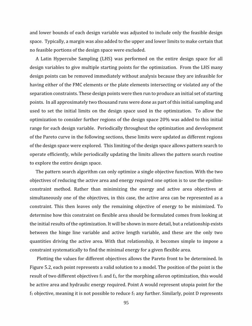
Figure 5.2: Generalized Pareto front. ............................................................................................ 96

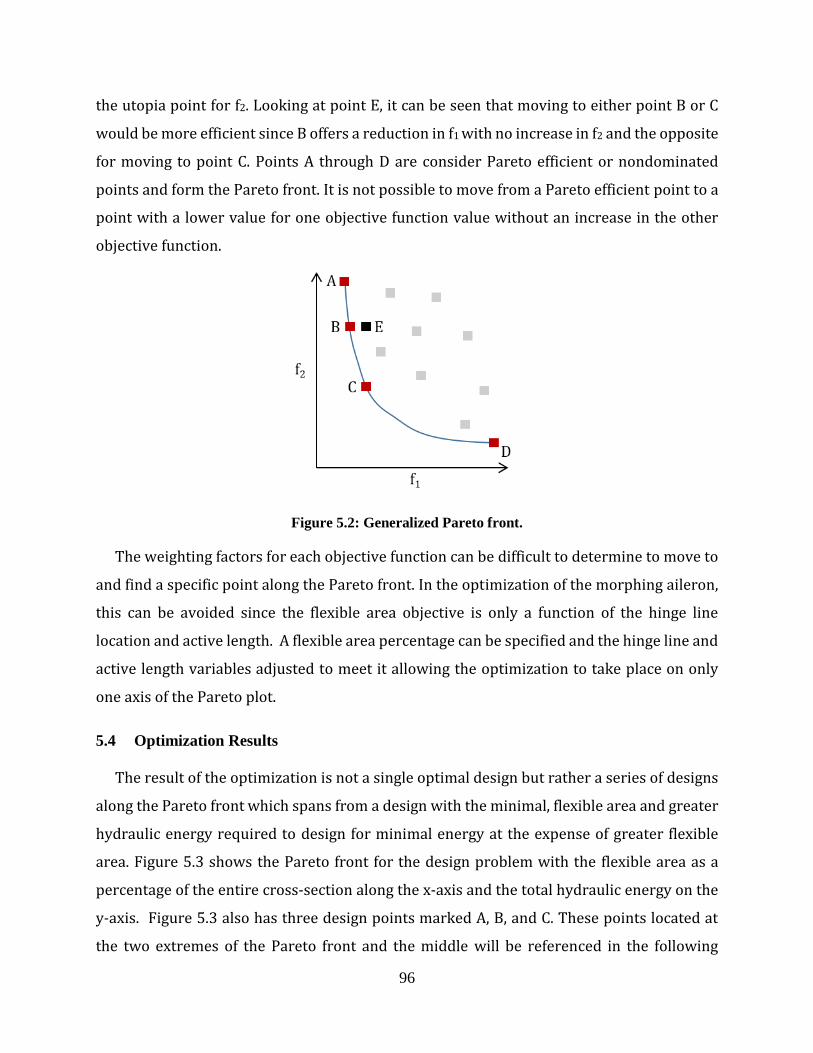
Figure 5.3: Optimization Pareto front for hydraulic energy and flexible area as a percentage of

the entire airfoil cross section ....................................................................................................... 97

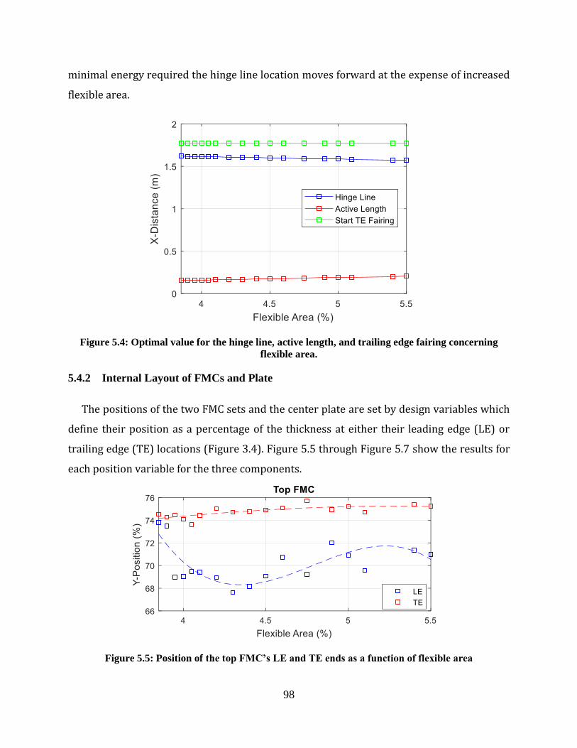
Figure 5.4: Optimal value for the hinge line, active length, and trailing edge fairing concerning

flexible area. .................................................................................................................................. 98

Figure 5.5: Position of the top FMC’s LE and TE ends as a function of flexible area ................. 98

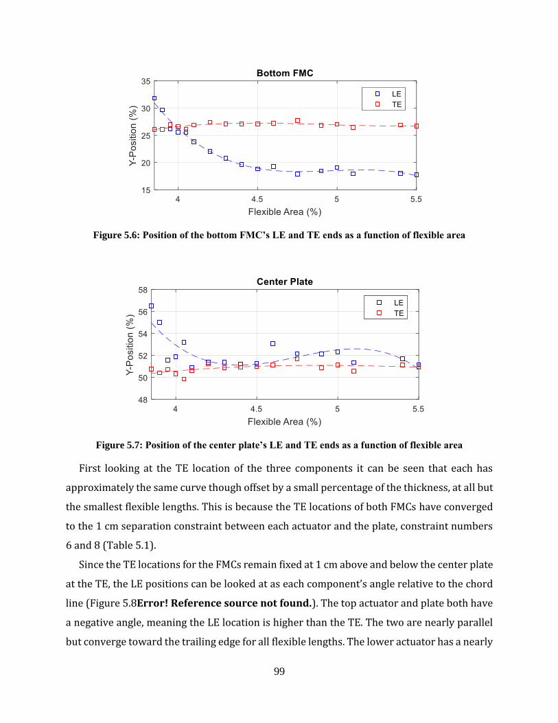
Figure 5.6: Position of the bottom FMC’s LE and TE ends as a function of flexible area .......... 99

Figure 5.7: Position of the center plate’s LE and TE ends as a function of flexible area ............. 99

Figure 5.8: Angle of internal components relative to the chord line. ......................................... 100

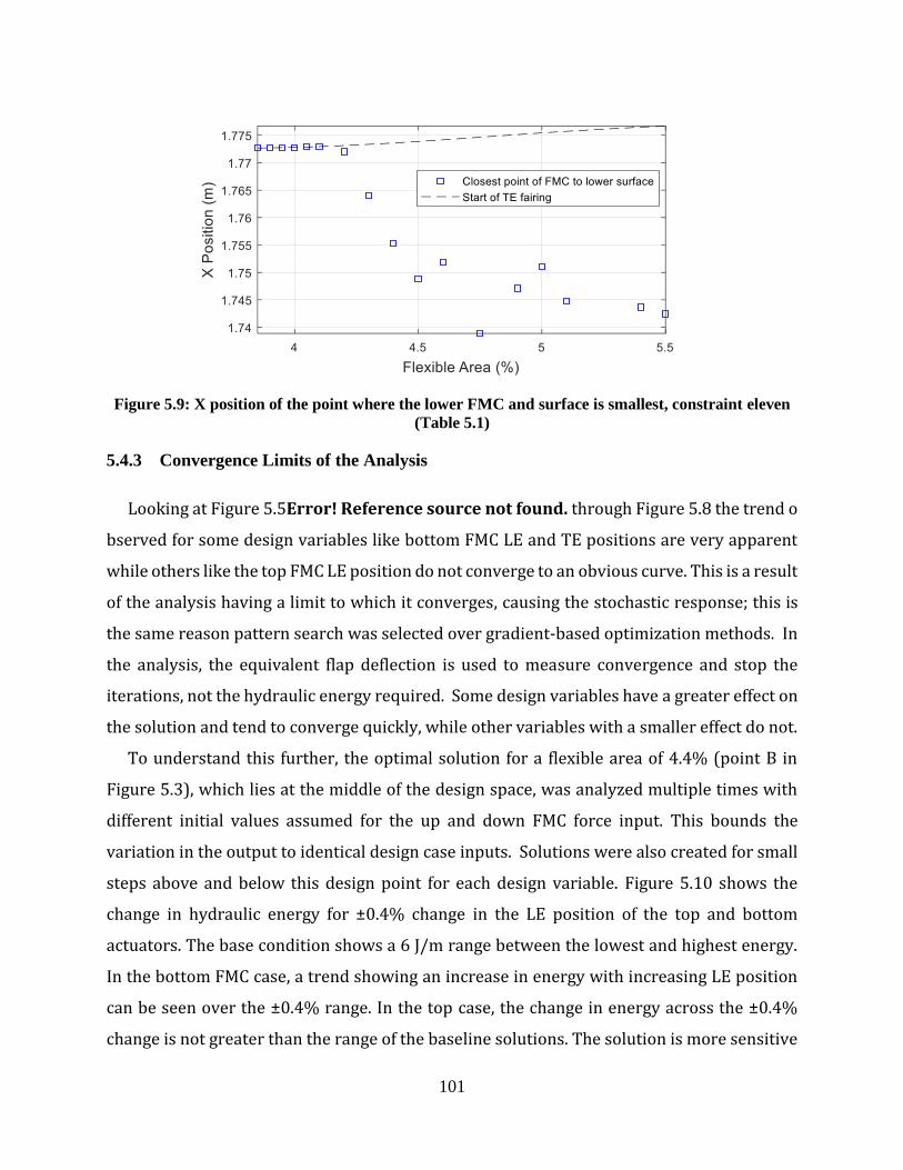
Figure 5.9: X position of the point where the lower FMC and surface is smallest, constraint

eleven (Table 5.1) ....................................................................................................................... 101

Figure 5.10: Effect of LE position of top and bottom FMC actuators ±0.4% from the baseline

condition of total hydraulic energy required ............................................................................... 102

Figure 5.11: Effect of plate thickness varying ±0.02 mm from the baseline condition on total

hydraulic energy required ........................................................................................................... 103

Figure 5.12: Contribution to bending stiffness of the center plate and inner and outer polymer

regions for optimal values along the Pareto front. ...................................................................... 104

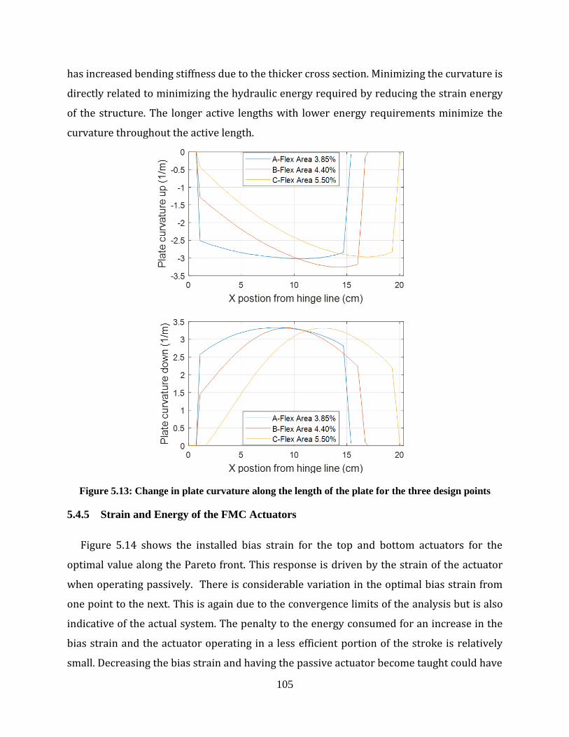
Figure 5.13: Change in plate curvature along the length of the plate for the three design points

..................................................................................................................................................... 105

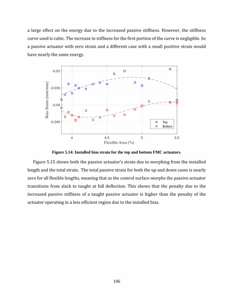
Figure 5.14: Installed bias strain for the top and bottom FMC actuators. .................................. 106

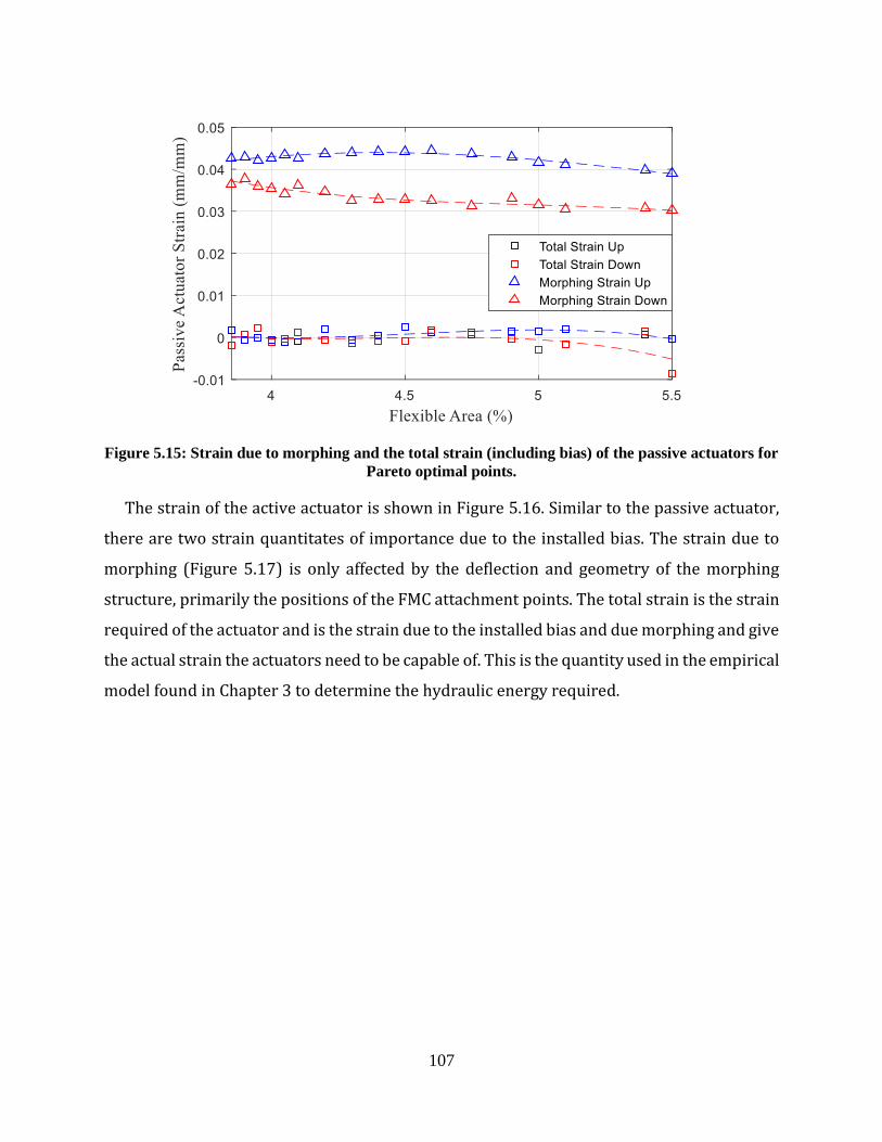
Figure 5.15: Strain due to morphing and the total strain (including bias) of the passive actuators

for Pareto optimal points. ............................................................................................................ 107

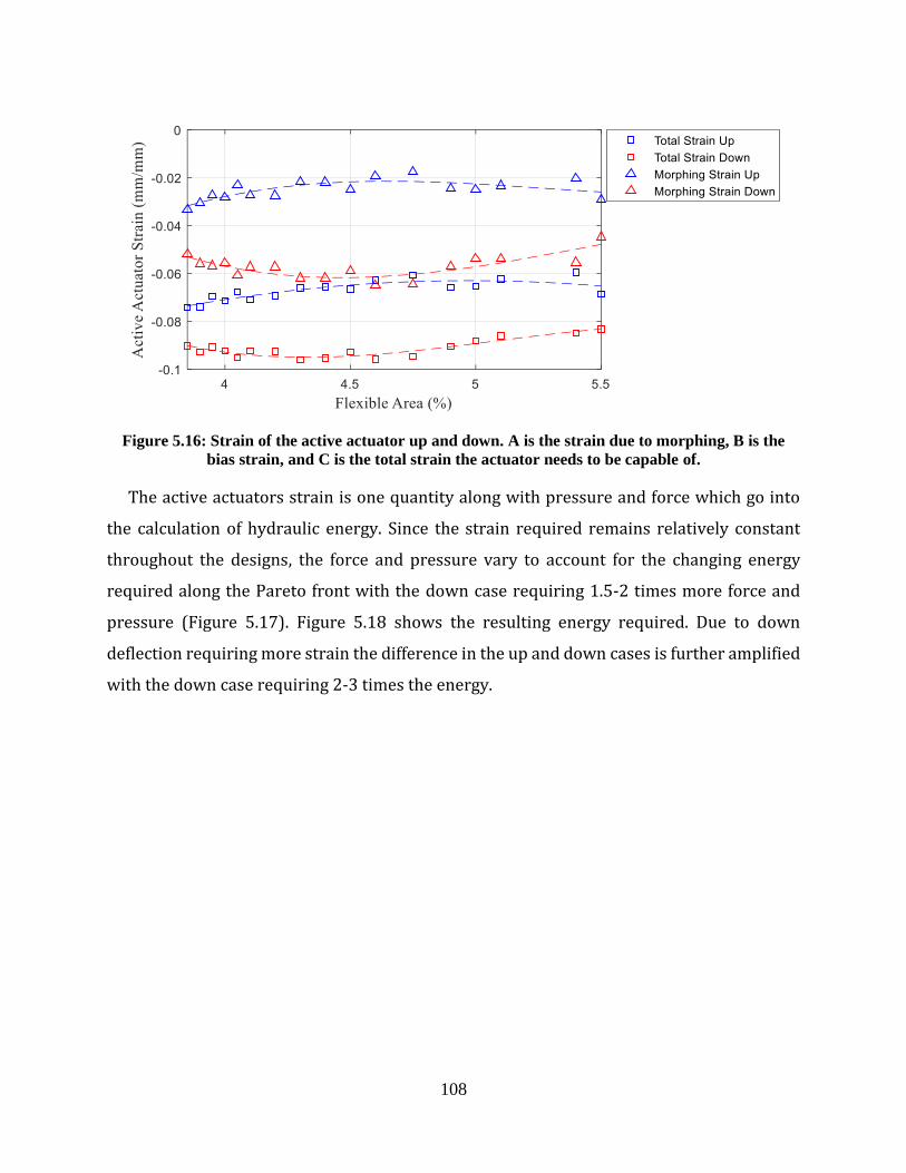
Figure 5.16: Strain of the active actuator up and down. A is the strain due to morphing, B is the

bias strain, and C is the total strain the actuator needs to be capable of. .................................... 108

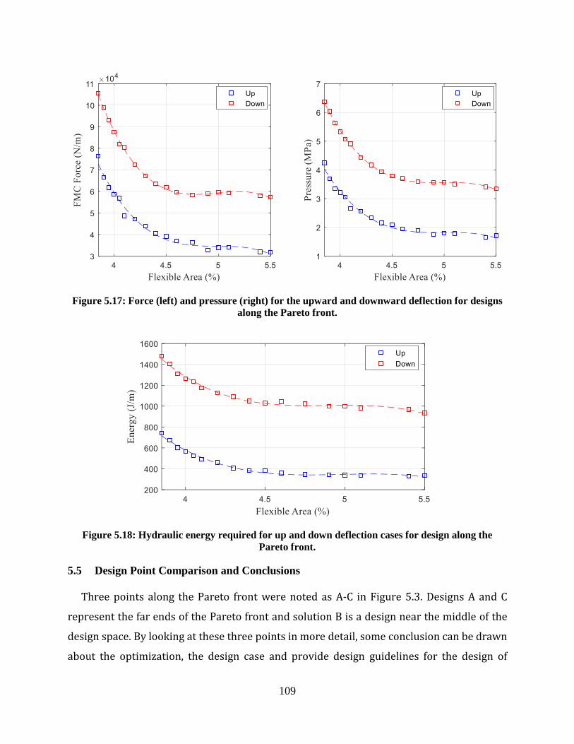
Figure 5.17: Force (left) and pressure (right) for the upward and downward deflection for designs

along the Pareto front. ................................................................................................................. 109

Figure 5.18: Hydraulic energy required for up and down deflection cases for design along the

Pareto front.................................................................................................................................. 109

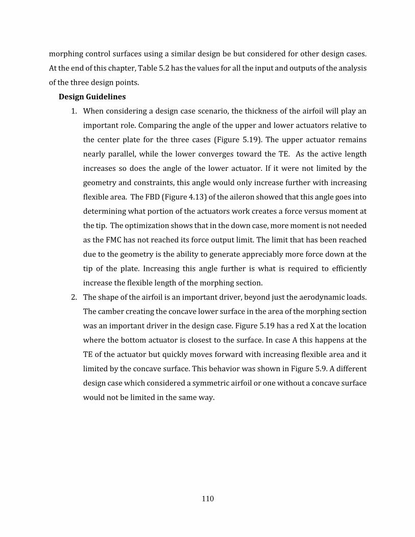
Figure 5.19: Internal layout of the three design points. .............................................................. 111

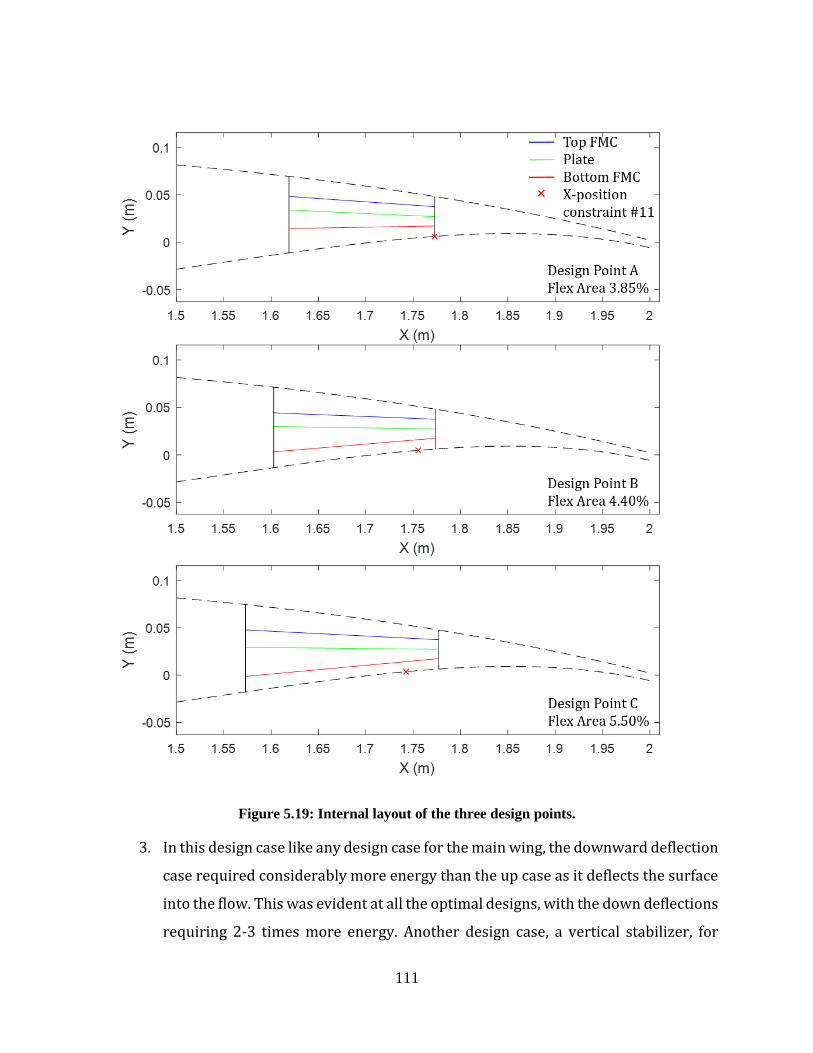
Figure 5.20: Up deflection for the three design points including center plate ............................ 112

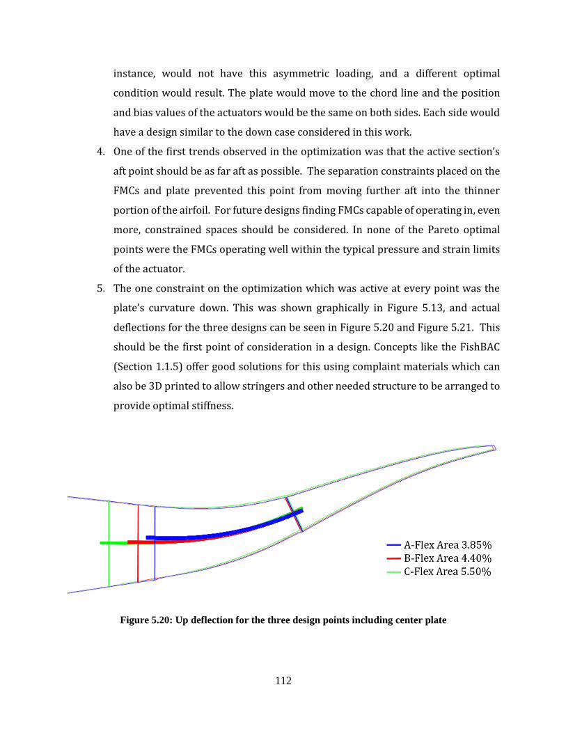
Figure 5.21: Down deflection for the three design points including center plate ....................... 113

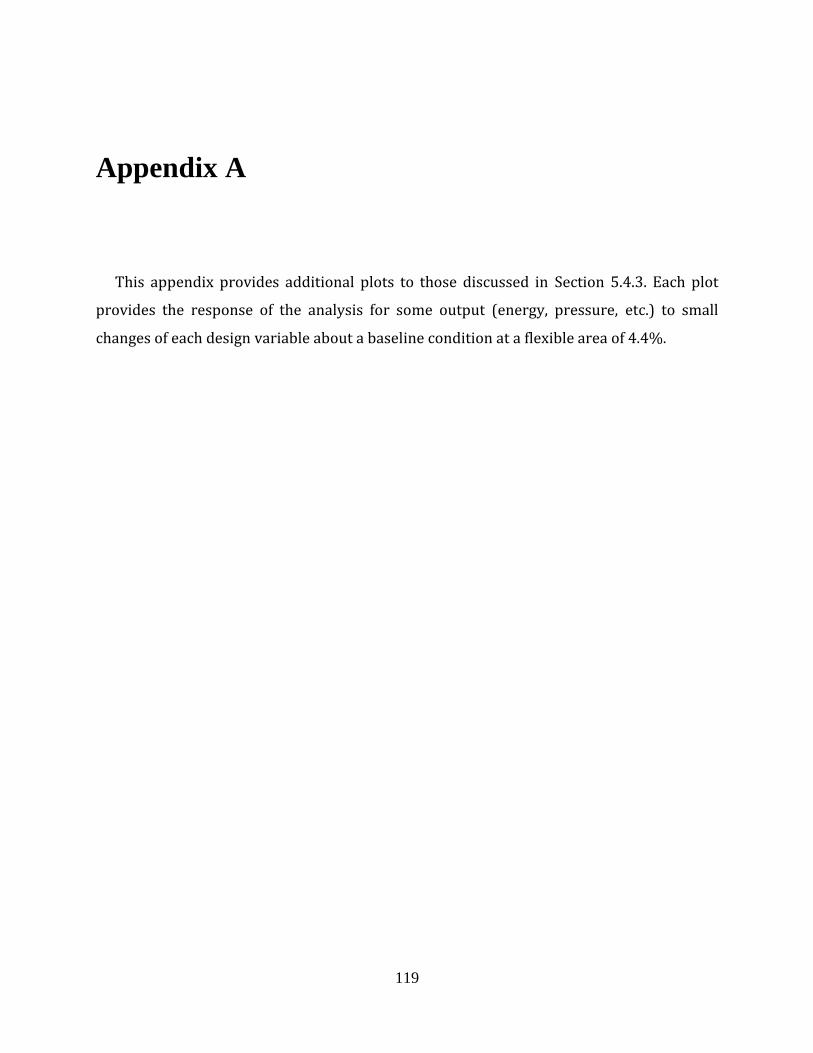
Figure A.1: Energy for the up deflection for small changes about the bassline case. ................ 120

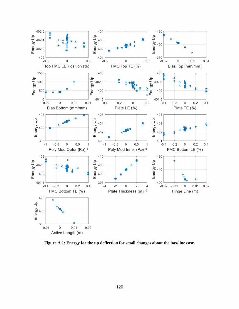
Figure A.2: Energy for the down deflection for small changes about the bassline case. ........... 121

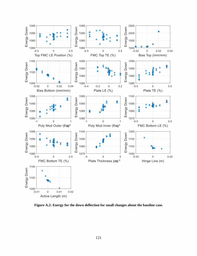
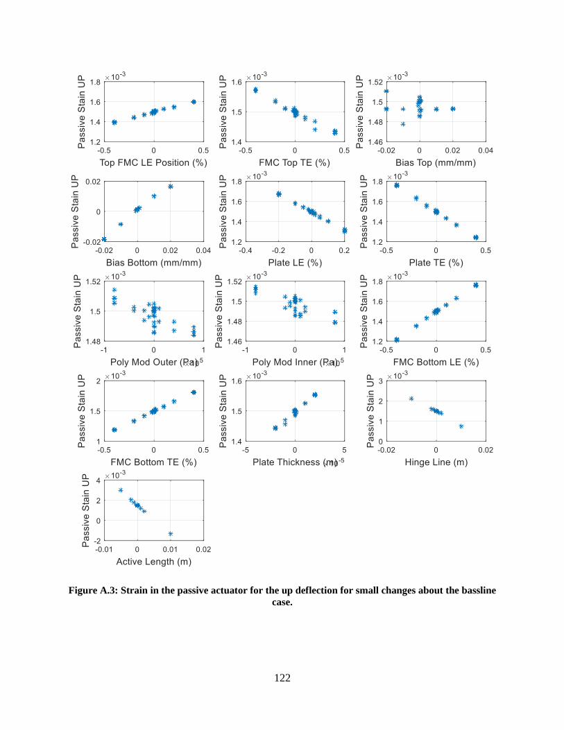
Figure A.3: Strain in the passive actuator for the up deflection for small changes about the

bassline case. ............................................................................................................................... 122

xiii

Figure A.4: Strain in the passive actuator for the down deflection for small changes about the

bassline case. ............................................................................................................................... 123

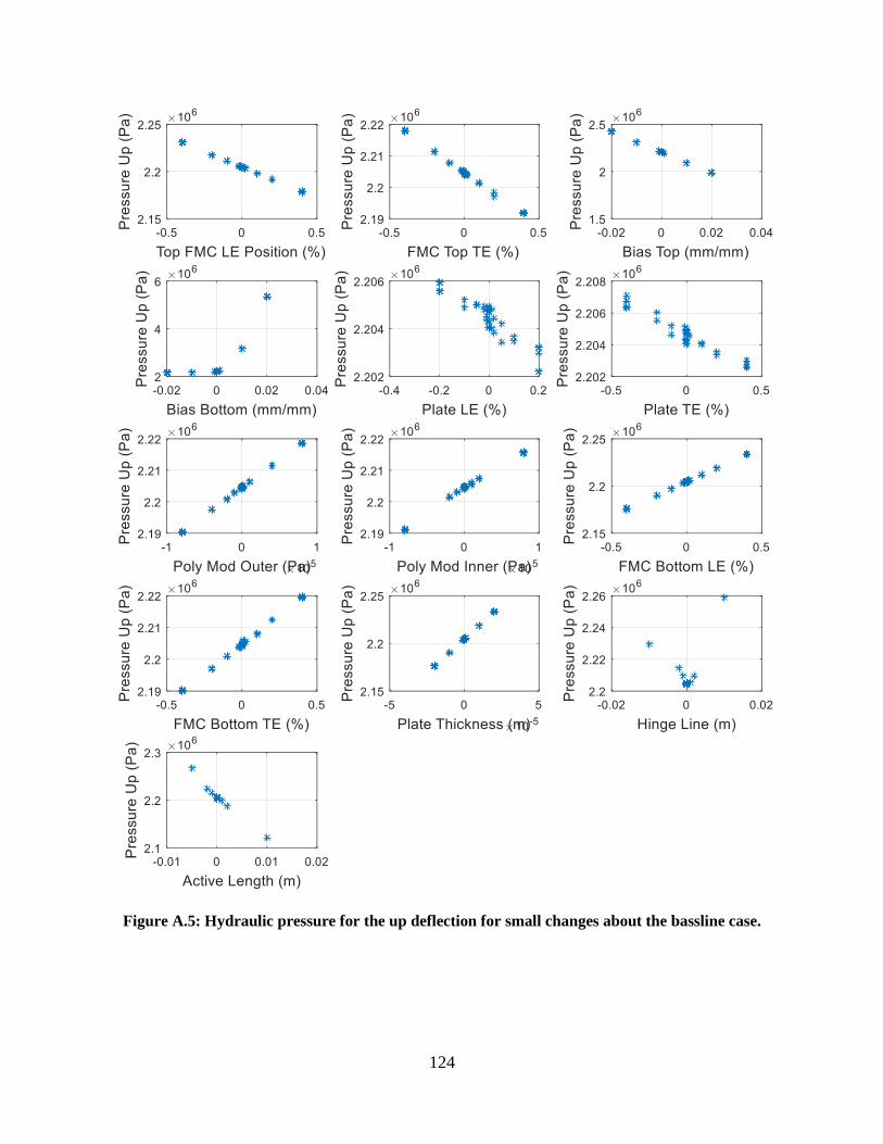
Figure A.5: Hydraulic pressure for the up deflection for small changes about the bassline case.

..................................................................................................................................................... 124

Figure A.6: Hydraulic pressure for the down deflection for small changes about the bassline case.

..................................................................................................................................................... 125

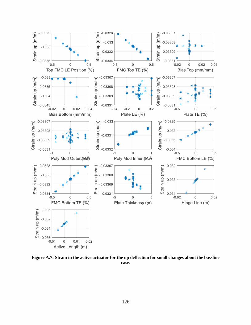
Figure A.7: Strain in the active actuator for the up deflection for small changes about the bassline

case. ............................................................................................................................................. 126

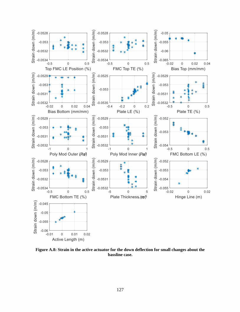
Figure A.8: Strain in the active actuator for the down deflection for small changes about the

bassline case. ............................................................................................................................... 127

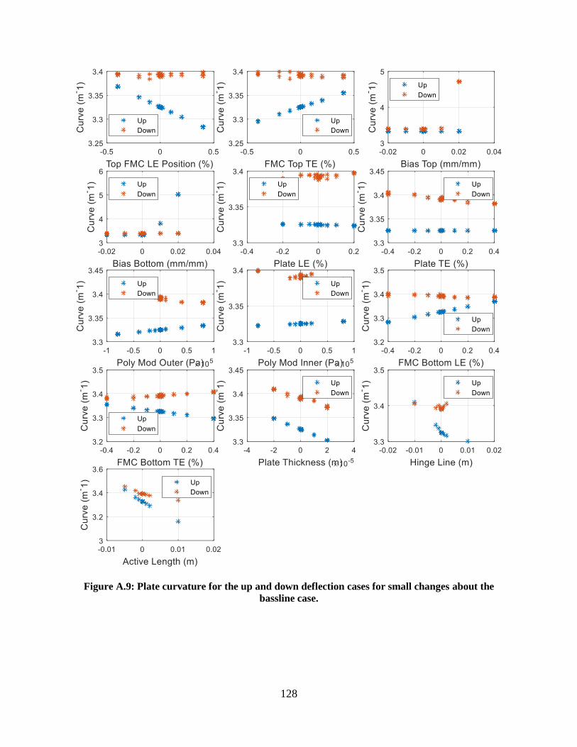
Figure A.9: Plate curvature for the up and down deflection cases for small changes about the

bassline case. ............................................................................................................................... 128

1

Chapter 1

1 Introduction and Literature Review

The idea of morphing aircraft control surfaces is as old as manned flight itself and was

born of necessity but quickly died out in favor of the simpler hinged flap. The idea has seen

periodic resurgence through history, mainly limited to research and with few designs

making it to production. Most recently, morphing aircraft control systems have seen a

resurgence as the development of small unmanned aerial vehicles (UAVs) offers the perfect

low-cost, low-risk platform. Interest has also grown as the aviation commercial transport

industry seeks increasingly efficient aircraft designs. These same aircraft manufacturers

also see increased pressure to reduce the noise signature of the aircraft as housing moves

closer to ever-growing airports. This dissertation looks at a design meant for manned

commercial transport aircraft, stepping far outside of the UAV scale of aircraft and unlike

many proposed designs, it uses a hydraulically driving actuators taking advantage of existing

hydraulic systems common to all modern commercial transport aircraft.

The actuation for the proposed design comes from Flexible Matrix Composite (FMC)

actuators, often thought of as hydraulically powered artificial muscles. Unlike conventional

servos or hydraulic pistons which require highly constrained rigid tracks, hinges, or

connector rods the FMC actuator can continue to actuate while bending and morphing with

the structure only needed to be secured at the two ends. The FMCs being considered in this

research operate at hydraulic pressures commonly found on modern commercial transport

aircraft.

This literature review will start by looking at the general concept of morphing aircraft

with previous examples ranging in size, flight speed, and technological maturity. The focus

is on designs that consider morphing for aircraft control purposes. The section following

will look at the development of the FMC actuator, its predecessors, and current models.

2

1.1 Morphing Aircraft Concepts

The term morphing as it relates to aircraft has been applied to a wide range of ideas and

designs. In the most general sense morphing is anything which changes the outer surface of

the aircraft for control or improvement in some performance metric like increased flight

envelope, efficiency, or noise reduction. Typically, this excludes devices which create

discontinuities in the surface like a conventional hinged control surface common to almost

all modern aircraft.

Currently, research in morphing aircraft concepts ranges in maturity from the earliest

concepts to manned flight-testing, and in scale from hand-launched UAVs to small business

jets. Just as varied is the approach to the design of the morphing structure and chosen

actuator. Morphing on a larger scale that involves significant changes in the camber [1-3],

wingspan [4-7], twist [8, 9], or sweep [10, 11] has been profoundly investigated since the

early 90’s with NASA’s Morphing Project [12]. Barbarino et al. published a compressive

review of these technologies through 2011 [13] and more recently by Sun et al. [14].

Although not the focus of this work, morphing for rotary wing aircraft is an important branch

of aviation-related morphing and Chopra and Giurgiutiu offer a review of those technologies

[15, 16].

While many have looked at morphing large portions of the aircraft’s wing, including

changes in the planform and twist, these all require significant reworking of how the aircraft

is designed and manufactured. A potential nearer term goal is the implementation of

morphing control surfaces. This approach calls for less change in the design process and

with some cases, like that presented in this paper can directly replace conventional control

surfaces even using existing hydraulic power sources.

A morphing control surface has two main advantages over a conventional hinged surface.

By eliminating the surface discontinuity, the aerodynamic characteristics of the profile can

be improved, and the acoustic emissions can be reduced. The following subsections will each

look at a different concept of morphing aircraft control surfaces. Each has a different

approach, method of actuation, reason for pursuing morphing, and different design cases.

3

1.1.1 The Origins of Morphing

Commonly the Wright Brothers, Orville, and Wilbur are referenced when discussing the

origins of wing morphing. The Wright Brothers who are credited with being the first to have

controlled powered flight overcame issues of roll control using morphing for their 1903

Wright Flyer (Figure 1.1)[17].

Figure 1.1: Picture of the 1903 Wright Flyer's Maiden Flight December 17th, 1903, Kitty Hawk NC

[18]

The biplane box structure of the Wright Flyer had relatively low torsional stiffness.

Instead of working to stiffen the structure further, they attached control lines running

diagonally across the wing’s structure. This allowed the pilot to twist the wings as a means

of roll control (Figure 1.2). The brothers received a patent for this aspect of the Wright Flyer

and referred to it as wing warping [19].

4

Figure 1.2: Top) 1903 Wright Flyer with warped wings [18] Bottom) Drawings from the Wright

Brother's first patent on wing warping [19].

While the Wright Brothers are certainly the first to employ wing warping successfully, the

idea itself predates their work. Weissharr et al. present some writings and a drawing of

Clements Ader’s Eole aircraft [20]. Ader’s proposed different roles for military aircraft and

described a wing that could change span in flight to allow the aircraft to achieve different

speeds.

By 1915 wing warping was out as the Fokler Eindecker was the last production plan to

use wing warping and even Orville Wright had begun using the conventional aileron for roll

control in his designs.

5

Figure 1.3: Clement Ader’s Eole concept from 1890 [21]

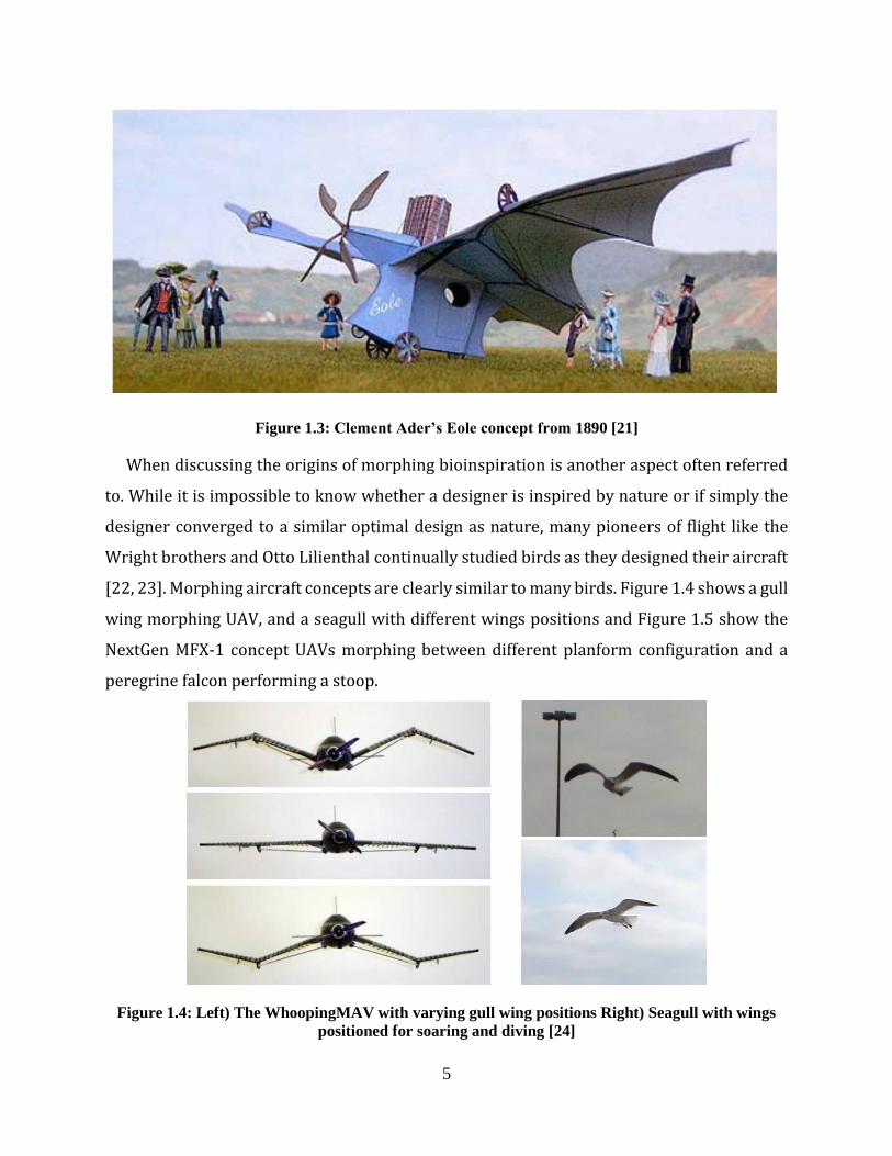
When discussing the origins of morphing bioinspiration is another aspect often referred

to. While it is impossible to know whether a designer is inspired by nature or if simply the

designer converged to a similar optimal design as nature, many pioneers of flight like the

Wright brothers and Otto Lilienthal continually studied birds as they designed their aircraft

[22, 23]. Morphing aircraft concepts are clearly similar to many birds. Figure 1.4 shows a gull

wing morphing UAV, and a seagull with different wings positions and Figure 1.5 show the

NextGen MFX-1 concept UAVs morphing between different planform configuration and a

peregrine falcon performing a stoop.

Figure 1.4: Left) The WhoopingMAV with varying gull wing positions Right) Seagull with wings

positioned for soaring and diving [24]

6

Figure 1.5: Left) NextGen MFX-1 UAV showing the two extremes of planform change[25], Right) A

peregrine falcon going from soaring to a steep dive in an action called a stoop

1.1.2 VCCTEF

The NASA Variable-Camber Continuous Trailing-Edge Flap (VCCTEF) concept originally

proposed by Nguyen [26] and has been studied by multiple groups [27, 28]. The concept is

based on NASA’s Generic Transport Model (GTM), a model representative of a modern

commercial airliner, without proprietary geometry. Instead of using the conventional

control surfaces of the GTM, the VCCTEF uses a series of distributed control surface across

nearly the entire trailing edge (Figure 1.6B). Each of these control surfaces is then divided

into several hinged segments in the chord direction (Figure 1.6A). When covered with a

highly compliant skin the discrete hinged control surfaces become one continuous morphing

surface.

7

Figure 1.6: A) three-part flap of the VCCTEF. B) Continuous trailing edge flap of the VCCTEF

with exaggerated deflections. [29]

Rodriguez et al. used the VCCTEF model and optimized flap positions for different off-

design conditions [29]. The idea is that a conventional wing is only optimal for one specific

flight condition, typically midcruise. As the aircraft burns fuel and changes weight the

optimal shape of the wing will also change from the beginning cruise condition to the end. It

was shown that the VCCTEF could optimize for each of these conditions by adjusting the flap

positions(Figure 1.7A). This results in a more optimal distribution of lift when compared to

the GTM with conventional control surfaces. Figure 1.7B shows the Cp distribution of the

conventional and morphing concepts and clearly showing a smoother more distributed

pressure for the morphing design.

Figure 1.7: A) Optimized flap position for the VCCTEF at four different flight conditions. B)

Pressure distribution on the top surface for the GTM and optimized VCCTEF at midcruise [29].

8

1.1.3 Piezoelectric Actuated Morphing Designs

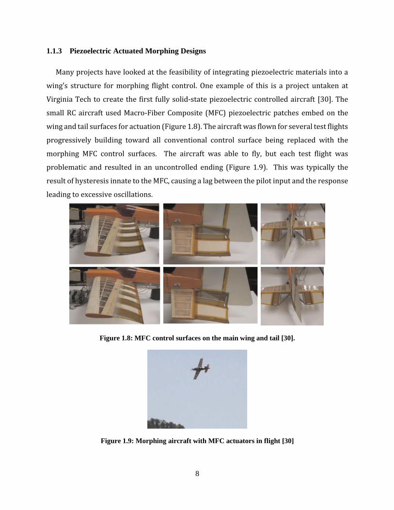
Many projects have looked at the feasibility of integrating piezoelectric materials into a

wing’s structure for morphing flight control. One example of this is a project untaken at

Virginia Tech to create the first fully solid-state piezoelectric controlled aircraft [30]. The

small RC aircraft used Macro-Fiber Composite (MFC) piezoelectric patches embed on the

wing and tail surfaces for actuation (Figure 1.8). The aircraft was flown for several test flights

progressively building toward all conventional control surface being replaced with the

morphing MFC control surfaces. The aircraft was able to fly, but each test flight was

problematic and resulted in an uncontrolled ending (Figure 1.9). This was typically the

result of hysteresis innate to the MFC, causing a lag between the pilot input and the response

leading to excessive oscillations.

Figure 1.8: MFC control surfaces on the main wing and tail [30].

Figure 1.9: Morphing aircraft with MFC actuators in flight [30]

9

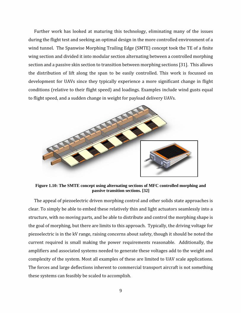
Further work has looked at maturing this technology, eliminating many of the issues

during the flight test and seeking an optimal design in the more controlled environment of a

wind tunnel. The Spanwise Morphing Trailing Edge (SMTE) concept took the TE of a finite

wing section and divided it into modular section alternating between a controlled morphing

section and a passive skin section to transition between morphing sections [31]. This allows

the distribution of lift along the span to be easily controlled. This work is focussed on

development for UAVs since they typically experience a more significant change in flight

conditions (relative to their flight speed) and loadings. Examples include wind gusts equal

to flight speed, and a sudden change in weight for payload delivery UAVs.

Figure 1.10: The SMTE concept using alternating sections of MFC controlled morphing and

passive transition sections. [32]

The appeal of piezoelectric driven morphing control and other solids state approaches is

clear. To simply be able to embed these relatively thin and light actuators seamlessly into a

structure, with no moving parts, and be able to distribute and control the morphing shape is

the goal of morphing, but there are limits to this approach. Typically, the driving voltage for

piezoelectric is in the kV range, raising concerns about safety, though it should be noted the

current required is small making the power requirements reasonable. Additionally, the

amplifiers and associated systems needed to generate these voltages add to the weight and

complexity of the system. Most all examples of these are limited to UAV scale applications.

The forces and large deflections inherent to commercial transport aircraft is not something

these systems can feasibly be scaled to accomplish.

10

1.1.4 UAV Flight Control With Twisting Acutation

When considering morphing for flight control, there are three fundamental shape changes

that can be done. A change in the camber of the entire airfoil, change in camber about a small

portion (typically the TE) or changing the angle of attack [33]. A group at the University of

Kentucky looked at demonstrating a morphing wing UAV in flight using this last approach of

changing the angle of attack or twisting the outboard section of the wing with the goal of

autonomous flight control.

Figure 1.11: Approaches to morphing for flight control: camber change (left), local camber change

(center), and angle of attack or twist (right) [34].

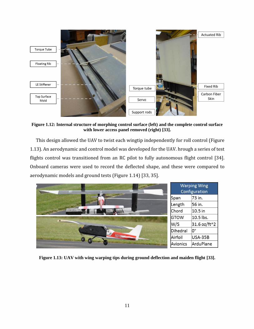
The design used an internal structure with sufficient bending stiffness to carry the wing

loading, but with very low torsional stiffness for actuation. This structure was then cast in

soft foam to form the aerodynamic surface (Figure 1.12 left). The torque tube, also serving

as the spar was only bonded to the outermost rib and not the foam allowing a continuous

curvature of the surface during actuation. Inboard of the morphing section the torque tube

was constrained by bushings and actuated with a conventional servo (Figure 1.12 right).

11

Figure 1.12: Internal structure of morphing control surface (left) and the complete control surface

with lower access panel removed (right) [33].

This design allowed the UAV to twist each wingtip independently for roll control (Figure

1.13). An aerodynamic and control model was developed for the UAV. hrough a series of test

flights control was transitioned from an RC pilot to fully autonomous flight control [34].

Onboard cameras were used to record the deflected shape, and these were compared to

aerodynamic models and ground tests (Figure 1.14) [33, 35].

Figure 1.13: UAV with wing warping tips during ground deflection and maiden flight [33].

12

Figure 1.14: LE and TE view of the left morphing surface during a right roll maneuver [33].

1.1.5 FishBAC

The Fish Bone Active Camber (FishBAC) concept uses a monolithic flexible structure

which resembles the skeleton of a fish creating a compliant structure which can be morphed

[36, 37] (Figure 1.15). The surface is created from pretension elastomer, and the structure

is controlled through tendons being actuated by a conventional servo. Through a fluid-

structure interaction model and later through wind tunnel testing, a 305 mm chord FishBAC

prototype was shown to have 20-25% increase in L/D when compared to best-case

conventional flap airfoil with sealed gaps and no external control horns or protrusions from

the surface [38].

Figure 1.15: A) FishBAC prototype and B) FishBAC concept [36].

Several different ideas for the structural layout of morphing control surfaces have been

investigated; a brief history of these was presented by Woods et al. [39] including the DARPA

Smart Wing which uses a layout similar to the one ultimately used for the morphing spoiler

concept presented in Chapter 2 [40].

A multi-objective optimization using genetic algorithms of the FishBAC was done [41].

Mass, drag, and actuation energy were considered as objectives and design variables allowed

the thickness of various components, number of stringers and the position of the morphing

13

section to be varied. The analysis consisted of XFOIL for the fluid solution and a Euler-

Bernoulli beam model to represent the skin and stringers stiffness. Serval Pareto fronts from

the optimization were presented. Figure 1.16A shows the Pareto front for the resulting drag

and energy results. The optimization had difficulty populating the lower drag portions of the

design space; this was attributed to issues innate to XFOIL. The authors note that change in

drag is much smaller than that seen for energy and mass for the Pareto efficient points. The

results for energy and mass (Figure 1.16B) shows a better-populated designs space and a

clear tradeoff is in the relationship between mass and energy. Energy is assumed here to be

proportional to the torque seen at the tendon pulley. This relationship in actuation energy

and mass of the structure is similar to that found as part of this dissertation for a morphing

FMC aileron in Chapter 5.4.

Figure 1.16: Pareto plots of optimal solutions for the FishBAC concept for the objective of mass,

drag, and actuation energy.

1.1.6 FlexSys

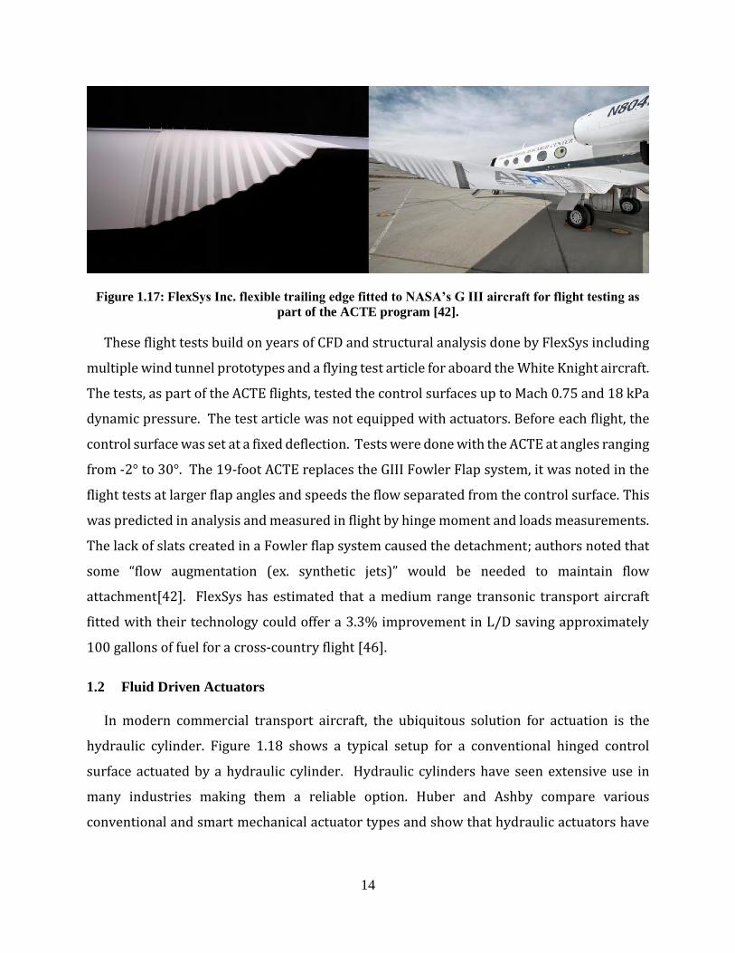
Recently FlexSys Inc. conducted a series of flight tests of a morphing control surface fitted

to a NASA Gulfstream G-III business jet as part of the Adaptive Compliant Trailing Edge

(ACTE) program [42]. FlexSys claims a 5-12% increase in range due to the aircraft always

being able to maintain an optimal configuration as the aircraft’s weight decreases due to fuel

burn [43]. At this time the exact method used for morphing is proprietary, but the company

has filed several patents [44, 45].

14

Figure 1.17: FlexSys Inc. flexible trailing edge fitted to NASA’s G III aircraft for flight testing as

part of the ACTE program [42].

These flight tests build on years of CFD and structural analysis done by FlexSys including

multiple wind tunnel prototypes and a flying test article for aboard the White Knight aircraft.

The tests, as part of the ACTE flights, tested the control surfaces up to Mach 0.75 and 18 kPa

dynamic pressure. The test article was not equipped with actuators. Before each flight, the

control surface was set at a fixed deflection. Tests were done with the ACTE at angles ranging

from -2° to 30°. The 19-foot ACTE replaces the GIII Fowler Flap system, it was noted in the

flight tests at larger flap angles and speeds the flow separated from the control surface. This

was predicted in analysis and measured in flight by hinge moment and loads measurements.

The lack of slats created in a Fowler flap system caused the detachment; authors noted that

some “flow augmentation (ex. synthetic jets)” would be needed to maintain flow

attachment[42]. FlexSys has estimated that a medium range transonic transport aircraft

fitted with their technology could offer a 3.3% improvement in L/D saving approximately

100 gallons of fuel for a cross-country flight [46].

1.2 Fluid Driven Actuators

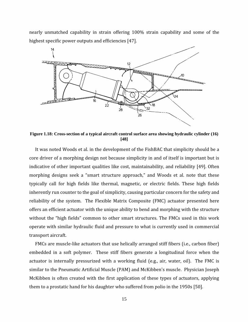
In modern commercial transport aircraft, the ubiquitous solution for actuation is the

hydraulic cylinder. Figure 1.18 shows a typical setup for a conventional hinged control

surface actuated by a hydraulic cylinder. Hydraulic cylinders have seen extensive use in

many industries making them a reliable option. Huber and Ashby compare various

conventional and smart mechanical actuator types and show that hydraulic actuators have

15

nearly unmatched capability in strain offering 100% strain capability and some of the

highest specific power outputs and efficiencies [47].

Figure 1.18: Cross-section of a typical aircraft control surface area showing hydraulic cylinder (16)

[48]

It was noted Woods et al. in the development of the FishBAC that simplicity should be a

core driver of a morphing design not because simplicity in and of itself is important but is

indicative of other important qualities like cost, maintainability, and reliability [49]. Often

morphing designs seek a “smart structure approach,” and Woods et al. note that these

typically call for high fields like thermal, magnetic, or electric fields. These high fields

inherently run counter to the goal of simplicity, causing particular concern for the safety and

reliability of the system. The Flexible Matrix Composite (FMC) actuator presented here

offers an efficient actuator with the unique ability to bend and morphing with the structure

without the “high fields” common to other smart structures. The FMCs used in this work

operate with similar hydraulic fluid and pressure to what is currently used in commercial

transport aircraft.

FMCs are muscle-like actuators that use helically arranged stiff fibers (i.e., carbon fiber)

embedded in a soft polymer. These stiff fibers generate a longitudinal force when the

actuator is internally pressurized with a working fluid (e.g., air, water, oil). The FMC is

similar to the Pneumatic Artificial Muscle (PAM) and McKibben's muscle. Physician Joseph

McKibben is often created with the first application of these types of actuators, applying

them to a prostatic hand for his daughter who suffered from polio in the 1950s [50].

16

In the 1980’s the Bridgestone Corporation began marketing the first commercial use of a

fluid-driven muscle, the “rubbertuator” [51]. It was marketed as an actuator for robots

operating in potentially explosive environments since no electrical components are needed.

Bridgestone stopped their “rubbertuator” work in the 1990s. Currently, the FESTO

Corporation has a commercial off the shelf option for pneumatic muscles [52]. A review of

previous work on FMC actuators and similar actuators through 2011 was presented by

Zhang [53].

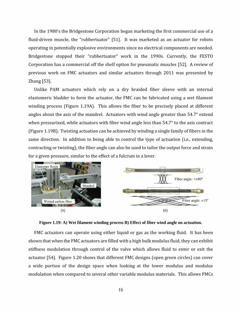
Unlike PAM actuators which rely on a dry braided fiber sleeve with an internal

elastomeric bladder to form the actuator, the FMC can be fabricated using a wet filament

winding process (Figure 1.19A). This allows the fiber to be precisely placed at different

angles about the axis of the mandrel. Actuators with wind angle greater than 54.7° extend

when pressurized, while actuators with fiber wind angle less than 54.7° to the axis contract

(Figure 1.19B). Twisting actuation can be achieved by winding a single family of fibers in the

same direction. In addition to being able to control the type of actuation (i.e., extending,

contracting or twisting), the fiber angle can also be used to tailor the output force and strain

for a given pressure, similar to the effect of a fulcrum in a lever.

Figure 1.19: A) Wet filament winding process B) Effect of fiber wind angle on actuation.

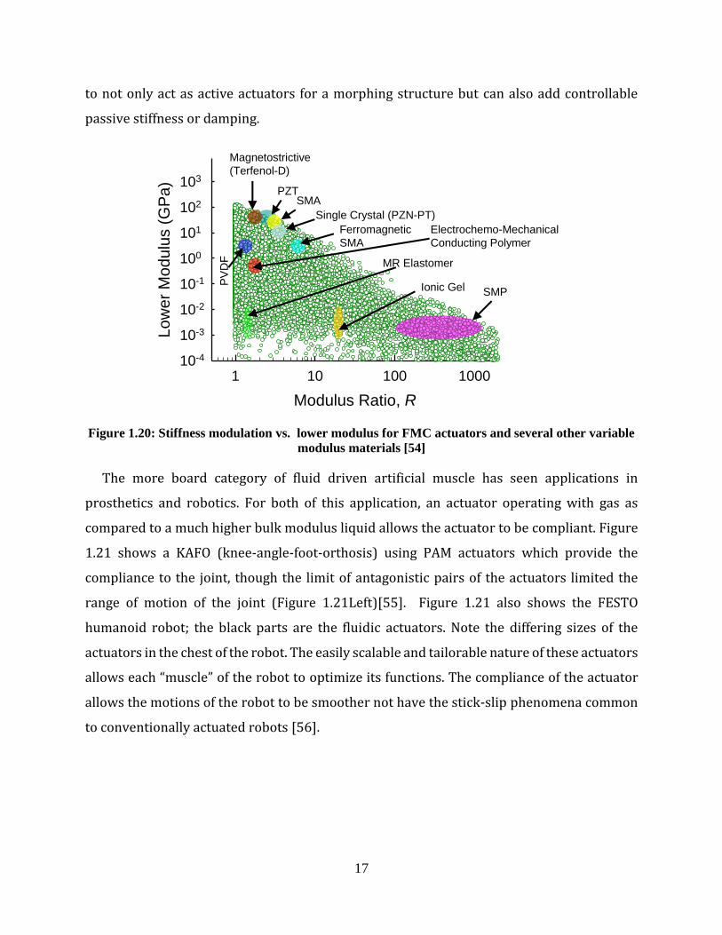
FMC actuators can operate using either liquid or gas as the working fluid. It has been

shown that when the FMC actuators are filled with a high bulk modulus fluid, they can exhibit

stiffness modulation through control of the valve which allows fluid to enter or exit the

actuator [54]. Figure 1.20 shows that different FMC designs (open green circles) can cover

a wide portion of the design space when looking at the lower modulus and modulus

modulation when compared to several other variable modulus materials. This allows FMCs

17

to not only act as active actuators for a morphing structure but can also add controllable

passive stiffness or damping.

Figure 1.20: Stiffness modulation vs. lower modulus for FMC actuators and several other variable

modulus materials [54]

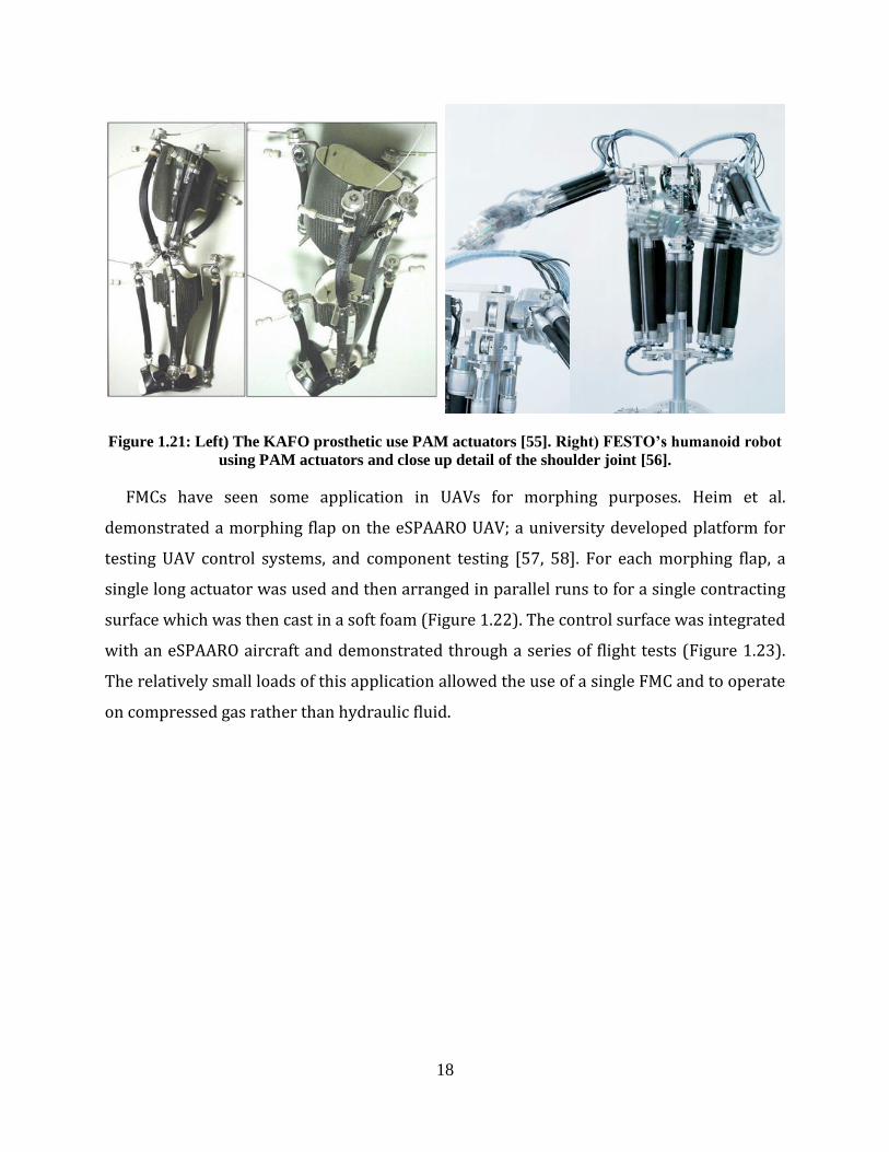
The more board category of fluid driven artificial muscle has seen applications in

prosthetics and robotics. For both of this application, an actuator operating with gas as

compared to a much higher bulk modulus liquid allows the actuator to be compliant. Figure

1.21 shows a KAFO (knee-angle-foot-orthosis) using PAM actuators which provide the

compliance to the joint, though the limit of antagonistic pairs of the actuators limited the

range of motion of the joint (Figure 1.21Left)[55]. Figure 1.21 also shows the FESTO

humanoid robot; the black parts are the fluidic actuators. Note the differing sizes of the

actuators in the chest of the robot. The easily scalable and tailorable nature of these actuators

allows each “muscle” of the robot to optimize its functions. The compliance of the actuator

allows the motions of the robot to be smoother not have the stick-slip phenomena common

to conventionally actuated robots [56].

Modulus Ratio, R

1 10 100 1000

Lo

we

r M

od

ulu

s (

GP

a)

10-4

10-3

10-2

10-1

100

101

102

103

SMP

SMAPZT

Magnetostrictive

(Terfenol-D)

Single Crystal (PZN-PT)

Ferromagnetic

SMA

Electrochemo-Mechanical

Conducting Polymer

Ionic Gel

MR Elastomer

PV

DF

18

Figure 1.21: Left) The KAFO prosthetic use PAM actuators [55]. Right) FESTO’s humanoid robot

using PAM actuators and close up detail of the shoulder joint [56].

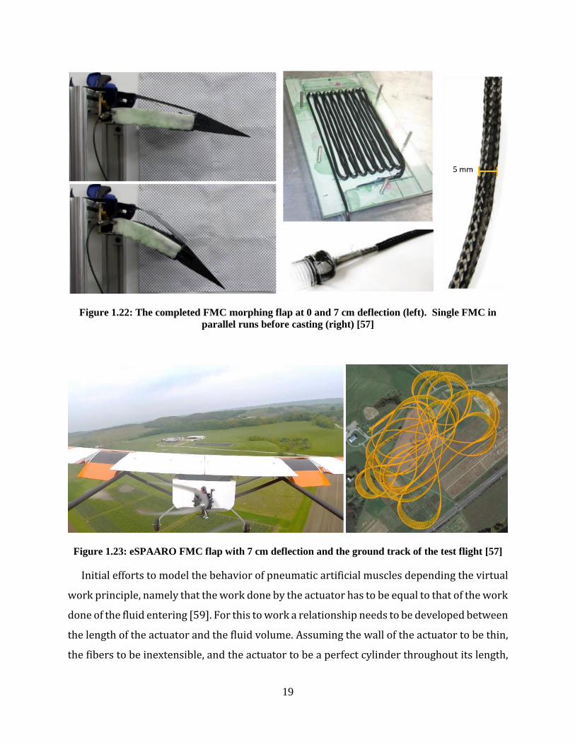
FMCs have seen some application in UAVs for morphing purposes. Heim et al.

demonstrated a morphing flap on the eSPAARO UAV; a university developed platform for

testing UAV control systems, and component testing [57, 58]. For each morphing flap, a

single long actuator was used and then arranged in parallel runs to for a single contracting

surface which was then cast in a soft foam (Figure 1.22). The control surface was integrated

with an eSPAARO aircraft and demonstrated through a series of flight tests (Figure 1.23).

The relatively small loads of this application allowed the use of a single FMC and to operate

on compressed gas rather than hydraulic fluid.

19

Figure 1.22: The completed FMC morphing flap at 0 and 7 cm deflection (left). Single FMC in

parallel runs before casting (right) [57]

Figure 1.23: eSPAARO FMC flap with 7 cm deflection and the ground track of the test flight [57]

Initial efforts to model the behavior of pneumatic artificial muscles depending the virtual

work principle, namely that the work done by the actuator has to be equal to that of the work

done of the fluid entering [59]. For this to work a relationship needs to be developed between

the length of the actuator and the fluid volume. Assuming the wall of the actuator to be thin,

the fibers to be inextensible, and the actuator to be a perfect cylinder throughout its length,

20

Equation (1-1) results. Where F is the force generated, D0 is the diameter when the wind

angle is 90°, P is the internal pressure, and θ is the fiber wind angle [59].

𝐹 =𝜋𝐷0

2𝑃

4(3 cos2 𝜃 − 1) (1-1)

This approach is limited since it does not consider many clearly important aspects of the

actuator, namely assuming the actuator to be a cylinder. The ends of the actuator are

typically swaged in an end fitting which forces each end to maintain the original diameter

during actuation. A review of modeling approaches for McKibben muscles was done by

Tondu [60]

A model proposed by Shan et al. allows for nonlinear analysis FMC actuators accounting

for many of the nonlinear effects not addressed in other models [54]. The model takes into

account the material as well as geometric nonlinearities associated with the large change in

shape the fibers and membrane undergo. This eliminates the need to model the actuator as

a perfect cylinder throughout its length and accurately capture the end effects. The model

also allows the extensibility of the fibers to be considered. The model was implemented in

the analysis of a sheet of parallel FMC tubes being used for a variable stiffness structure [54]

and as part of a novel actuator inspired by plants fibrillar networks with the internal

pressure controlled by electroosmotic transport mechanism [61].

1.3 Motivation and Dissertation Outline

Each of the previously discussed designs undoubtedly contributes to different aspects of

morphing for aircraft control. Each also has its limits, creating small gaps in the technology.

That is the motivation of this dissertation. The Wright brothers and bioinspiration started

the very idea of morphing, but their wing warping was born more of out of necessity and

opportunity than purposeful design and was quickly replaced by the conventional aileron as

flight speeds increased. The VCCTEF studies show the possible benefits in commercial

transport aircraft, but it is limited to a paper study only. Little consideration is given as to

exactly how the morphing surfaces could be designed, actuated, and implemented. The

FishBAC concept and others tested on UAVs provide insight into different designs and novel

ways to go about morphing, but the scale of aircraft, which allows that line of research to be

so dynamic also limits its application in manned flight. The FlexSys ACTE flight tests show

21

promise in the future of morphing designs for manned aircraft, but many questions remain

unanswered about the actual design. Unlike the previously mentioned morphing projects

scaled for UAVs, the ACTE offers a straightforward application to manned flight, but this also

hampers the ability of the research to explore new designs. Though little is known about the

inner workings of the ACTE, it is known that the design uses “conventional” actuators. The

next generation of morphing designs should not be limited to actuators of the past. This work

aims to explore a morphing aircraft design for commercial transport aircraft, using novel

methods of actuation, while considering and demonstrating the design beyond paper studies

alone through benchtop prototypes.

This dissertation consists of six chapters, which are organized as follows.

The first chapter introduces background information on morphing aircraft specifically

looking at control surfaces, actuation methods, and structural layout. Additionally,

background on the flexible matrix composite actuator (FMC) is presented.

The second chapter discusses the use of FMC in a morphing active spoiler for use in a

commercial aircraft. A functional prototype was fabricated and tested demonstrating, that

FMCs can be used in morning control surface.

Based on the concept of the active spoiler, the third chapter looks at the challenges of

designing an FMC morphing aileron. An analysis combining structural, fluid, and actuator

models is presented.

The fourth chapter takes the model developed in the prior chapter and looks at the effect

that each of the design variables has on the morphing aileron. Trend plots show how the

design changes throughout the design space.

The fifth chapter looks at how to optimize the morphing FMC aileron for a particular

design case and presents not only the solution to this particular design case but also

guidelines for adapting the FMC aileron to other control surface position and design cases.

The final chapter summarizes the work done and looks at possible areas for future work.

22

Chapter 2

2 Design and Testing of a Morphing FMC Spoiler

One of the motivations and goals of this research is to demonstrate the morphing FMC

actuator control surface concept through full-scale benchtop prototypes. This chapter will

look at the development of a high performance morphing spoiler for air gap control with a

deployed Fowler flap using pressurized flexible matrix composites (FMC) actuators (Figure

2.1). This design takes the surface normally used as a spoiler to dump lift and allow it to

control the gap between it and the deployed Fowler flap for increased flow control. More

specifically, the objectives are to (1) design an FMC morphing spoiler control surface, (2)

fabricate a full-scale prototype, (3) achieve the performance requirements under expected

aerodynamic loading, and to (4) demonstrate closed-loop control for position control. For

objective (3) based on requirements provided by the sponsor, the spoiler needed to be able

to achieve 12 cm of tip deflection under anticipated aerodynamic load with closed-loop

control. Using a morphing spoiler allows the gap between what would normally be the fixed

portion of the wing and a deployed Fowler flap to be controlled. This has the potential to

increase flap performance, reduce acoustic emissions and reduce overall system weight by

potentially eliminating a panel from the Fowler flap system and reducing the size of the

kinematic tracks mechanism.

The approach for meeting the technical objectives are to employ a series of finite element

(FE) models to analyze, perform studies, and access performance considering different

configurations to yield a final design. Next, the fabrication and testing of individual FMC

actuators were performed to characterize the actuation response and test for failure before

being installed in the prototype spoiler. The final phase of the work was the fabrication and

testing of a full-size prototype morphing spoiler. A series of tests were performed to look at

23

the spoiler’s: passive stiffness, deflection under different simulated aerodynamic loads, and

closed-loop control under different loading conditions.

Figure 2.1: Morphing Spoiler Concept

2.1 Model-Based Design

As specified in the performance requirements, deflection was required in only one

direction for the morphing control surface, and thus the basic concept for the morphing

spoiler control surface used extending actuators near the top surface and contracting

actuators near the bottom surface (Figure 2.1). Several versions of the morphing spoiler

design were considered utilizing a series of finite element models, and the results of these

models guided the design process leading to the final design that was fabricated and tested.

The morphing spoiler has three basic sections as highlighted in Figure 2.2. The manifold

assembly provided the hydraulic pressure and mounting point for the FMC actuators. The

active portion of the actuators were embedded in a deformable material and thus referred

to as the active section in this paper. As the spoiler’s thickness decreases approaching the

trailing edge, there was a location where the FMCs could no longer physically fit. At this

location, the rigid trailing edge fairing completes the profile.

The FE model used a 2D analysis of the spoiler employing Abaqus CAE plane strain

elements (CPE3 and CPE4) using the nonlinear geometry solution. Using this 2D approach

allowed for multiple designs to be considered efficiently with minimum computational time.

The spoiler’s profile was first partitioned into the three basic areas of the spoiler: manifold,

an active region, and trailing edge section (Figure 2.2). Attachment points were also

designated on the manifold and trailing edge section that allowed following surface traction

forces to be applied representing the FMC actuators. The spoiler is 50 cm in the chord

Flap

Contracting

FMC actuators

Extensional

FMC actuators

Wing

Flap

Wing trailing

edge (spoiler)

24

direction, and the position of the FMC aft mount points was set at 38 cm aft of the manifold

where the spoiler has a thickness of 4 cm. This is a minimum thickness of the spoiler at which

the FMCs could be mounted due to space constraints.

Figure 2.2: Partitioned and meshed FE model

The intent of this analysis was to determine the material and structural layout that

generated the required forces and displacements to meet performance specifications. For

this reason, the FMCs themselves were not modeled, but rather loads were applied at the

attachment points. Once loads were determined, then estimations of required actuation

pressure could be determined using actuator characterization data collected from

experiments.

The first design considered the entire active section cast in a polyurethane rubber (Shore

A-80 hardness, E=6.7 MPa). The first loading condition considered a blocked condition

where the trailing edge was constrained to have zero vertical motion (Figure 2.3A). As the

loads representing the FMCs were increased, the resulting force generated at the trailing

edge was measured. Before the loads could be increased to even a small fraction of the FMC’s

maximum output, the model showed significant undesired deflections (Figure 2.3B).

Figure 2.3: A) Boundary conditions and loads for blocked case. B) First design iteration showing

undesired deflection

25

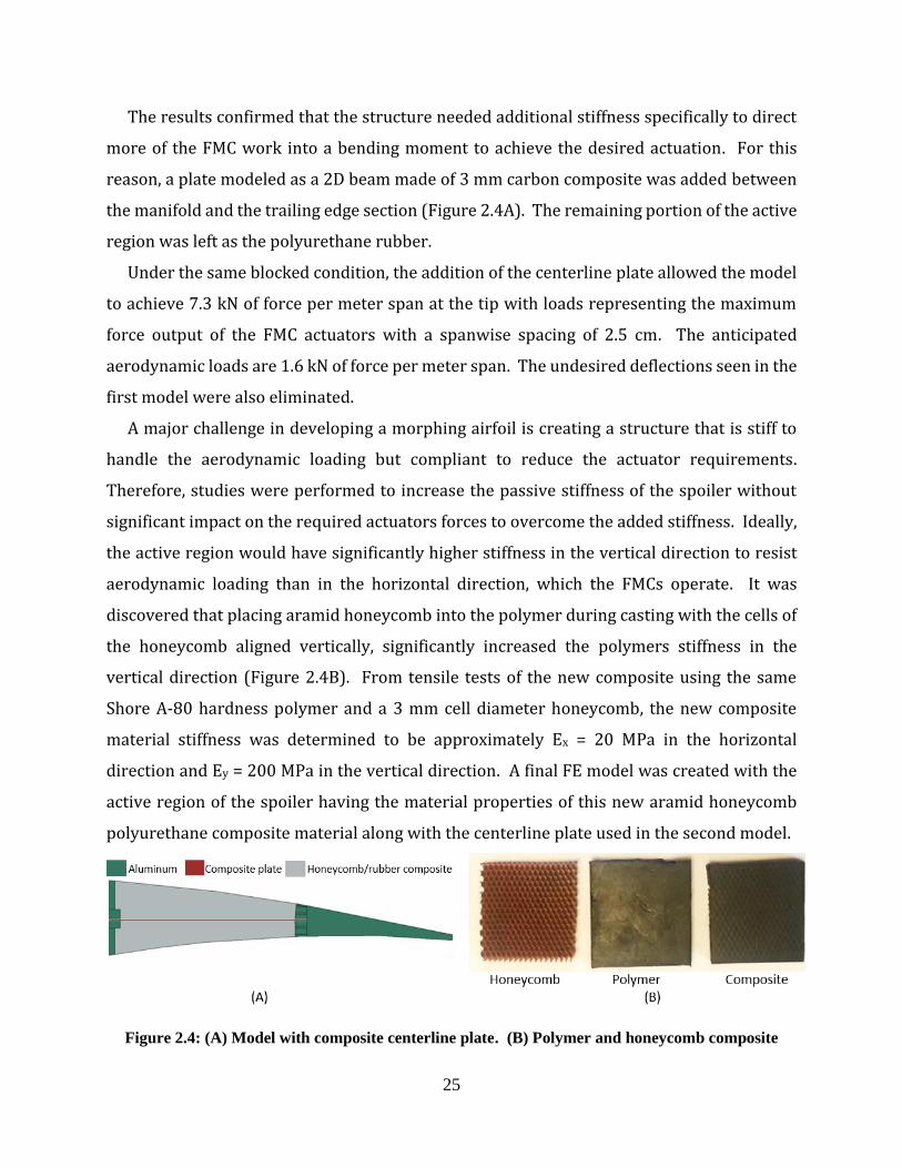
The results confirmed that the structure needed additional stiffness specifically to direct

more of the FMC work into a bending moment to achieve the desired actuation. For this

reason, a plate modeled as a 2D beam made of 3 mm carbon composite was added between

the manifold and the trailing edge section (Figure 2.4A). The remaining portion of the active

region was left as the polyurethane rubber.

Under the same blocked condition, the addition of the centerline plate allowed the model

to achieve 7.3 kN of force per meter span at the tip with loads representing the maximum

force output of the FMC actuators with a spanwise spacing of 2.5 cm. The anticipated

aerodynamic loads are 1.6 kN of force per meter span. The undesired deflections seen in the

first model were also eliminated.

A major challenge in developing a morphing airfoil is creating a structure that is stiff to

handle the aerodynamic loading but compliant to reduce the actuator requirements.

Therefore, studies were performed to increase the passive stiffness of the spoiler without

significant impact on the required actuators forces to overcome the added stiffness. Ideally,

the active region would have significantly higher stiffness in the vertical direction to resist

aerodynamic loading than in the horizontal direction, which the FMCs operate. It was

discovered that placing aramid honeycomb into the polymer during casting with the cells of

the honeycomb aligned vertically, significantly increased the polymers stiffness in the

vertical direction (Figure 2.4B). From tensile tests of the new composite using the same

Shore A-80 hardness polymer and a 3 mm cell diameter honeycomb, the new composite

material stiffness was determined to be approximately Ex = 20 MPa in the horizontal

direction and Ey = 200 MPa in the vertical direction. A final FE model was created with the

active region of the spoiler having the material properties of this new aramid honeycomb

polyurethane composite material along with the centerline plate used in the second model.

Figure 2.4: (A) Model with composite centerline plate. (B) Polymer and honeycomb composite

26

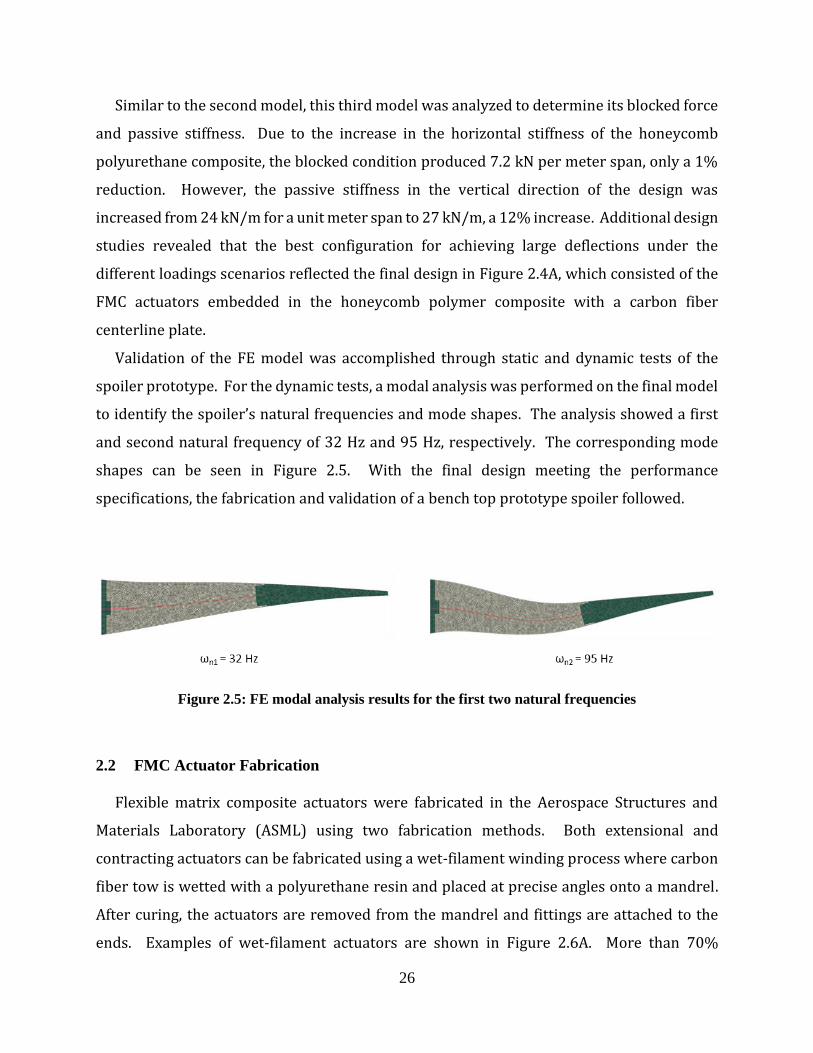
Similar to the second model, this third model was analyzed to determine its blocked force

and passive stiffness. Due to the increase in the horizontal stiffness of the honeycomb

polyurethane composite, the blocked condition produced 7.2 kN per meter span, only a 1%

reduction. However, the passive stiffness in the vertical direction of the design was

increased from 24 kN/m for a unit meter span to 27 kN/m, a 12% increase. Additional design

studies revealed that the best configuration for achieving large deflections under the

different loadings scenarios reflected the final design in Figure 2.4A, which consisted of the

FMC actuators embedded in the honeycomb polymer composite with a carbon fiber

centerline plate.

Validation of the FE model was accomplished through static and dynamic tests of the

spoiler prototype. For the dynamic tests, a modal analysis was performed on the final model

to identify the spoiler’s natural frequencies and mode shapes. The analysis showed a first

and second natural frequency of 32 Hz and 95 Hz, respectively. The corresponding mode

shapes can be seen in Figure 2.5. With the final design meeting the performance

specifications, the fabrication and validation of a bench top prototype spoiler followed.

Figure 2.5: FE modal analysis results for the first two natural frequencies

2.2 FMC Actuator Fabrication

Flexible matrix composite actuators were fabricated in the Aerospace Structures and

Materials Laboratory (ASML) using two fabrication methods. Both extensional and

contracting actuators can be fabricated using a wet-filament winding process where carbon

fiber tow is wetted with a polyurethane resin and placed at precise angles onto a mandrel.

After curing, the actuators are removed from the mandrel and fittings are attached to the

ends. Examples of wet-filament actuators are shown in Figure 2.6A. More than 70%

27

actuation strain has been achieved with the extensional actuators, and 25%-30% actuation

strains are typical with contracting actuators. Another fabrication method for creating FMC

actuators uses a dry braided sleeve with an inner bladder that is later cast in a polymer resin,

forming the FMC actuator. The advantage of this technique is the increased bond strength

of the dry sleeve with the metal fitting using epoxy (e.g. 3M DP460). Under high loads and

pressures, the wet-filament wound actuators are more likely to fail due to the poor bonding

between the composite laminate having a soft polymer and the metal fittings. The actuators

selected for the spoiler were sized (diameter) based on the anticipated force requirements

in the FE model. The contracting actuators fabricated using the dry braided sleeve method

had a wind angle of ±15º which has been shown to provide large forces and displacements

[62]. All actuators are pressurized to approximately 5 MPa in a blocked setup prior to casting

into the final system, and forces exceeding 4000 N are typically measured. Figure 2.6B shows

a typical force vs. displacement curve for an FMC actuator. The lines of constant pressure

were obtained using a pneumatic regulator to maintain constant pressure. For safety

concerns, the blocked values at the higher pressures were obtained using a hydraulic hand

pump. However, due to limitations of the hydraulic setup, it was not possible to get lines of

constant pressure at values greater than 1.0 MPa.

Figure 2.6: (A) Example FMC actuators – actuators are fabricated using wet-filament winding

process, and dry braided sleeves later cast in a polymer resin and (B) Typical force and strain

results for an actuator at constant pressure and in a blocked condition.

28

2.3 Active Spoiler Prototype

To demonstrate the use of FMCs in the morphing control surface a functional, full-scale

prototype of the active spoiler was created. Through a series of benchtop tests, the spoiler

was shown to meet the design requirements for deflection, load, and to be closed-loop

controlled.

2.3.1 Design and Fabrication

The morphing spoiler prototype was fabricated to match the full-scale profile with a

length of 0.6 m. The span dimension was set at 0.13 m, representing a portion of the full

span. The active spoiler consists of a custom manifold, FMC actuators, perforated carbon

fiber centerline plate, and an aramid honeycomb core (Figure 2.7A). An aluminum mount

was CNC machined for mounting the active spoiler, and a rapid-prototyped tail section was

fabricated using 3D printing. In this prototype, five extensional actuators were placed on

top, and the same number of contracting actuators were placed on the bottom (Figure 2.7B).

The extensional actuators were made from the wet filament winding process, and braided

aramid sleeves were used for the contracting actuators. Based on the FE models a centerline

carbon fiber plate was added. Before casting the polymer to form the spoiler the region

between the centerline plate and the FMC actuators was filled with strips of 3 mm diameter

12.7 mm thickness aramid honeycomb (Figure 2.7C). For casting, a mold of the spoiler’s

outer mold line was 3D printed and the active region filled with PMC-780 polyurethane

rubber. During curing, the entire section was kept under vacuum to remove entrapped air

and ensure that honeycomb had no voids. A black pigment was used in the polymer, and the

spoiler tip was painted black for better visibility (Figure 2.7D). The final mass of the active

section was 8.29 kg.

29

Figure 2.7: (A) Designed spoiler prototype, (B) assembled spoiler before casting without

honeycomb core (C) active spoiler with honeycomb core before casting and (D) active spoiler after

casting in PMC 780 polyurethane

2.3.2 Quasistatic Experiments

The first tests performed with the prototype were quasi-static tests to determine the

relationships between hydraulic pressurization of the FMC actuators, tip displacement, and

force. In these tests, the FMC actuators were slowly pressurized using a hydraulic hand

pump; the tip displacement was measured using an ADMET testing frame extensometer, and

the pressure measured with an Ashcroft 2000 psig pressure transducer. The results showed

a nearly linear relationship of 1.6 cm/MPa and the spoiler was able to achieve 12 cm of tip

deflection (Figure 2.8A).

Using the ADMET testing frame with a 4.4 kN load cell, force measurements were taken

with the active spoiler blocked at three different tip positions, i.e. 0 cm, 6 cm, and 10 cm, as

shown in Figure 2.8B. The spoiler was attached to the load cell on the ADMET testing frame

using a carbon fiber cable. This cable was then connected at the end of the active section,

just before the rapid prototyped tail section, as shown in Figure 2.9A. Similar to the

displacement measurement, the hand pump was used to slowly pressurize the actuators

30

while the testing frame held the spoiler stationary. Pressure and force were simultaneously

measured. In most cases, 400 N stationary force was achieved, which is approximately 2.5

times the estimated aerodynamic loading for a similarly sized spoiler in the span and chord

directions.

Figure 2.8: (A) Tip free displacement with increased actuation pressure and (B) measured force of

the spoiler at different constrained tip displacements

Passive stiffness experiments were performed to determine the unpressurized stiffness

of the spoiler. The test setup shown in Figure 2.9A was used to obtain the force to

displacement measurement without pressurizing the actuators. The force was recorded at

the end of the spoiler was raised using the testing frame with the carbon fiber cable. The

results show that there was very little tip deformation even with a 400 N force. The

experimental results showed the spoiler to be 12% stiffer than the FE model, and one

possible reason is that the stiffness of the actuators was not included in the model (Figure

2.9B). Even though the deflections were small, one can use the actuators to compensate for

any undesired deflections and return the spoiler to the original configuration. During

deflections, some spanwise deflections were observed due to Poisson’s effect during larger

deflections of the spoiler and these deflections were small relative to the spoiler’s width.

31

Figure 2.9: (A) Force measurement testing setup and (B) unpressurized stiffness result

2.3.3 Dynamic Testing of the Active Spoiler and FE Validation

For the dynamic testing to validate the natural frequencies calculated from the FE model,

the spoiler was excited by a shaker while the valve to the manifold was closed. Before closing

the valve, the actuators were pressurized to different values to determine the effects of the

internal pressure on frequency response. For these tests, the active spoiler was mounted

inverted to allow for easier positioning of the shaker. A LDS V408 vibration shaker with

PA100E Power Amplifier was used to excite the spoiler, and a PCB 221A04 force transducer

(1.1218 mV/N) provided force measurement between the spoiler and shaker (Figure 2.10).

Pressure via an Ashcroft 2000 psig pressure transducer was placed on a tee fitting between

the closed valve and the spoiler manifold. Tip velocity was measured using a Polytec laser

vibrometer (Figure 2.10). A National Instruments system with a PXI-4461 (24-Bit, 204.8 kS/s,

2-Input/2-Output) and a PXI-4462 (24-Bit, 204.8 kS /s 4-Input) data acquisition module

recorded the force, velocity, and pressure as well as provides the output signal for the shaker.

The Sound and Vibration Measurement Suite in LabVIEW 2010 was used for calculating the

results, displaying the data, and recording the data for importing into Matlab. The sampling

rate for the data acquisition system was set to 1000 Hz, a Hanning window was used for the

spectral analysis, and a bandwidth-limited random noise signal was used for providing the

excitation signal to the vibration shaker. A total of 10 averages were performed for

computing the frequency response of the system at each internal pressure.

32

Figure 2.10. Experiment setup for dynamic system analysis

Prior to the start of each run, the actuators were pressurized with a hand pump to the

desired pressure and then the valve shut. Figure 2.11A shows the response of tip velocity

over the applied load from the shaker. It shows a first natural frequency for each pressure

to be near 30 Hz, which corresponds well to the first bending mode of 32 Hz found in the FE

model. Additionally, a second resonant frequency appears close to the 95 Hz predicted. Also,

the natural frequency increases with increased initial pressure. In Philen (2012), it was

shown that the internal pressure could be used for tuning the stiffness of an FMC semi-active

isolation mount [63]. Similarly, these results confirm that the natural frequency of the active

spoiler can be altered by adjusting the internal pressure. Figure 2.11B shows the response

of the hydraulic pressure of the closed system over the applied load. While the first

structural natural frequency of 30 Hz does not appear in the pressure response, the 95 Hz

natural frequency can be seen in the pressure results, showing a stronger coupling between

the structure and hydraulic fluid.

Force Transducer

NI Dynamic

Signal Analysis System

LDS Shaker

Laser Vibrometer

Pressure Transducer

Laser Target

33

Figure 2.11: (A) Frequency response of tip velocity to the applied force for different initial

pressures. With an increase in pressure, the first resonant frequency is increasing. (B) Frequency

response of internal pressure to the applied force for different initial pressures.

2.3.4 System identification and closed-loop results for the active spoiler

Due to the complexities in modeling the dynamics of the morphing spoiler, hydraulic

pump, the servo-valve, and the response of the fluid in the hydraulic lines, it was decided to

perform a system identification of the entire system from the input control voltage to the

servo-valve to the output response of the morphing spoiler control surface. This also

avoided the complexities in trying to perform system identification of each component,

which would have required additional instrumentation unavailable in the lab.

To measure displacement during the tests, flex sensors manufactured by Spectra Symbol

were bonded using flexible silicone to the top surface of the active section (Figure 2.12A).

The flex sensors change resistance based on curvature. The flex sensors were calibrated

using displacements measured with a string wound around a rotary encoder, giving a

resolution of 0.6 mm. Instead of a hand pump, a compact hydraulic pump manufactured by

Marathon Electric was used to drive hydraulic fluid through a Parker D1FM servo-valve. To

evaluate the performance of the closed-loop system under loading, a spring (k= 8.75 kN/m)

was attached to the same anchor point used in the in the blocked and passive stiffness tests.

To measure the applied load, a 2.2 kN load cell was attached in line with the spring (Figure

2.12B).

34

Figure 2.12: Experiment setup for open and closed-loop results: (A) Spoiler showing location of flex

sensor and attachment of string at tip of spoiler and (B) images of hardware for conducting the

experiments

A dSpace™ control system using the 1103 board recorded the position from the rotary

encoder, voltage from flex sensors using a voltage divider circuit, and pressure from the

Ashcroft 2000 psig pressure transducer located near the spoiler’s manifold. The dSpace

system was used to control a Parker DFM1 servo spool valve for the open-loop and closed-

loop experiments. Shown in Figure 2.13 is a picture of the active spoiler achieving 14 cm of

tip displacement when unloaded.

Figure 2.13: Frame from video showing the active spoiler achieving 14 cm of tip displacement

Figure 2.14A shows the open-loop results for the unloaded spoiler with a sinusoidal input

to the servo spool valve. For the loaded case with the spring attached, the spoiler was still

able to achieve the 12 cm tip displacement requirement even under 600 N loading at max

deflection (Figure 2.14B).

35

Figure 2.14: Open-loop results for spoiler under cyclic testing: (A) Unloaded: Displacement (solid

blue), Pressure (dashed red) and (B) Loaded: Displacement (solid blue), Force (dashed red)

System identification was performed using input-output frequency response results to

acquire a Single Input Single Output (SISO) analytical model which was used to design the

feedback controller. To obtain the frequency responses of the active spoiler, the servo-valve

was controlled using the National Instruments PXI system with a PXI-4461 (24-Bit, 204.8

kS/s, 2-Input/2-Output). The hydraulic system was excited with a bandwidth limited

random noise signal with a -0.5 V bias being sent to the servo-valve. The bias prevents the

continual slow pressurization of the system due to the natural leakage of fluid through the

spool valves. The laser vibrometer and pressure transducers recorded tip velocity and

pressure, respectively. The sampling rate for the data acquisition system was set to 1000 Hz,

and a Hanning window was used for the spectral analysis. A total of 10 averages were

performed for computing the frequency response of the system. Shown in Figure 2.15 are

the experimentally obtained frequency response results and the identified analytical models.

Figure 2.15A is the output tip velocity in reference to the applied voltage to the servo-valve,

and Figure 2.15B is the output tip velocity in reference to the actuation pressure. The

identified transfer function was computed using the prediction error estimate function (PEM)

in Matlab and is shown in (2.1). This transfer function represents the output tip

displacement to the input voltage to the servo-valve and was obtained by integrating the

identified model shown in Figure 2.15A.

36

Figure 2.15 Frequency response of tip velocity to (A) servo-valve control voltage and (B) actuation

pressure. Blue: Identified system model and Red: Experiment

1 6 2 5 5 4

8 3 11 2 13 1 16

7 2 6 5 5 8 4

10 3 13 2 15 1

3.3763 10 2.3458 10 2.1858 10

3.3237 10 1.4227 10 4.8408 10 1.7652 10

1.0000 5.5481 10 5.9944 10 2.2491 10

8.3285 10 1.9515 10 2.3632 10 3.910

p

s s s

s s sG

s s s s

s s s

171 10

(2.1)

Using the root locus control design technique, a proportional controller having a gain of

5.6 was chosen based upon the desired bandwidth, pole locations, and step response. Shown

in Figure 2.16A is the root-locus for the system, which highlights a stable control region for

a gain range between 0 and 11.73. The effect of integral and derivative controllers was

examined in the analysis, but the objective of this work was to demonstrate accurate tracking

using a simple control system. Future work will investigate more advanced control

algorithms. Figure 2.16B is the closed-loop frequency response for the simple proportional

controller, where the input is the desired tip displacement, and output is actual tip

displacement. Accurate tracking of the desired displacement can be achieved at low

frequencies (input-output ratio is equal to 1 (0 dB) ), and the bandwidth of the system is

approximately 30 Hz.

37

Figure 2.16: (A) Root locus plot of identified plant in Eq. 1 (Maximum proportional gain 11.73)

and (B) frequency response of closed-loop system with proportional gain of 5.6

The feedback control system for position control was programmed using Simulink and

compiled with the Real-Time Workshop, which was downloaded onto the dSpace control

system. For feedback, the calibrated flex sensors attached to the active spoiler were used to

provide the position. Shown in Figure 2.17 are the closed-loop results for the active spoiler

when tracking step displacements between 0 and 12 cm. Figure 2.17A is the tip

displacement, and Figure 2.17B is the control voltage sent to the servo-valve. As seen, there

is good agreement between the analysis and experiment and the system can effectively track

the desired positions with a short response time.

For the loaded case the spring was again attached to the spoiler to resist its motion. The

results in Figure 2.18 demonstrate that the spoiler can effectively track the desired positions

under loading conditions. The small hysteresis seen in the deflection when returning to zero

is primarily due to the limitations of the hydraulic system to drain the fluid during

depressurization. Larger hydraulic lines or the addition of drain valves would mitigate this

further. The spoiler was able to exceed 300 N at 10 cm of deflection. The small local noise

seen in the results is primarily a result of the flex sensor used as the displacement sensor in

the control loop. The flex sensor embedded along the top surface change resistance was

converted to a DC voltage signal for dSpace through a voltage divider. Thus, the relatively

small change in resistance and the use of a simple voltage divider circuit resulted in signal

noise. However, the results demonstrate that accurate tracking control using a simple

38

control system is achievable even under pseudo-aerodynamic loading, and future work will

explore additional control algorithms for improved performance.

Figure 2.17: (A) Closed-loop results for spoiler tracking step displacements between 0 and 12 cm:

Desired displacement (solid blue), simulation results (red) and experiment (green) and (B) Control

output to servovalve: simulation (blue) and experiment (red)

Figure 2.18. Closed-loop results for the loaded spoiler tracking step displacements between 0 and

12 cm: (a) Desired displacement (solid blue), Actual displacement (dashed red) and (b) Control

output to servovalve (solid blue), Pressure (dashed red)

2.4 Active spoiler conclusions

This chapter looked at the design and demonstration of a high-performance actuation

system for morphing spoiler control using pressurized FMC actuators. Various types of

actuators were fabricated and tested under high pressures and loadings to examine their

performance capabilities. Using simplified 2D finite element models, multiple spoiler

39

designs were considered. The models identified the benefit of the composite centerline plate

to allow the FMC’s actuation to be efficiently converted into the desired morphing shape and

the benefit of using the anisotropic materials properties of the honeycomb polyurethane

composite to increase the passive stiffness of the structure.

A final prototype spoiler was created to evaluate the performance in a full-scale design.

The final prototype was full scale in the chord direction and was cast to match the actual

design scenario’s spoiler profile. The final prototype was first tested to determine its

maximum displacement and performance under pseudo-aerodynamic loading. The second

series of tests focused on the dynamic characteristics of the spoiler. Finally, a feedback

controller was designed, and the spoiler was able to be controlled and perform well while

loaded with pseudo-aerodynamic loads. To accompany this, an analytic model of the

system’s response was identified to allow for further analysis of the spoiler’s performance.

This chapter demonstrated through a benchtop prototype that a morphing aircraft

control surface actuated by FMCs is viable for commercial transport aircraft. To further

study this a more detailed analysis model is needed which can take into account the

nonlinear nature of the large defections needed, the energy requirements of the FMCs,

aerodynamic loading and allow for optimization of the design. Additionally, considering

control surfaces which are bidirectional will allow more advanced designs to be considered.

40

Chapter 3

3 Model Development for the Morphing FMC Aileron

The active spoiler concept from the previous chapter demonstrated through a benchtop

prototype and testing how FMCs can be used to create a morphing aircraft control surface

for a commercial transport aircraft. Motivated by the active spoiler work, this chapter and

following chapters look to further the FMC morphing aircraft control surface concept by

developing a model which can be used to optimize the design.

This new analysis includes a coupled structural, fluid and actuator models and is intended

to be a medium fidelity analysis to provide meaningful insight into the design and still be

computationally efficient for use in the optimization. The coupled fluid model allows for the

pressure on the morphing surface to be included in the structural model. An actuator model

based on empirical data is used to accurately take into account the fluid volume, pressure,

and energy requirements of the FMCs.

The model uses contracting actuators in antagonistic pairs to allow for deflection in two

directions in both the up and down direction. This expands the possible applications from

single direction actuation like the spoiler to now consider any flight control surface.

3.1 Design Case Definition and Design Variables

For this model, a specific design case was developed which focused on analyzing a

morphing aileron FMC control surface for a commercial transport aircraft. The initial

concept is similar to the previously discussed FMC morphing spoiler but with the upper

extending actuators replaced by contracting actuators which then operate as antagonistic

sets of contracting actuators. The aileron will deflect up when the top FMC set is pressurized

and down when the lower set of FMCs is pressurized. The model is parametrized allowing

for changes in the structural layout, material properties, FMC parameters, and loading

41

conditions. This parametrized model allows many designs to be considered efficiently to

determine an optimal design.

For this design case, the outboard section of the NASA Common Research Model (CRM)

was select (Figure 3.1). The CRM was developed by NASA to provide a standard set of

geometries, wind tunnel test data, and computational models that researchers could use

when researching modern medium size commercial transport aircraft since the geometries

of current commercial aircraft are often proprietary. The main wing of the CRM uses

multiple profiles; the one selected for this work is the outboard section where conventional

ailerons are located. The same model was used in the VCCTEF work discussed in Section

1.1.2 and seen in Figure 1.6.

Figure 3.1: A) Computational and wind tunnel models of the NASA CRM aircraft [64] [65].

Figure 3.2: Airfoil profile of the outboard section of the NASA CRM main wing.

With the goal of investigating the use of morphing FMC actuator control surface on a

commercial transport aircraft, several other parameters were chosen and presented in

(Table 3.1). The flight conditions and required deflection were selected based on typical

conditions for a commercial transport aircraft.

42

Table 3.1: Aileron case parameters

Design Case Parameters

Chord Length 2 m

Altitude 11 km

Velocity 231 m/s

Atmospheric Pressure 23.5 kPa

Dynamic Pressure 11.0 kPa

Flap Deflection ±20°

The basic concept of the morphing aileron was to be similar to the morphing spoiler, but

the analysis focuses on parameterized design variables related to the structural layout,

materials properties, and the FMC actuators themselves. Looking at an entire cross-section

of the wing it can be broken down into three major sections (Figure 3.3). First, the forward

portion of the wing that remains unchanged from a conventional aileron. Second, the active

portion that will deform for morphing, and finally the trailing edge fairing; which will move

with the active section but is considered a rigid piece. The line separating the active section

from the forward section will be referred to as the hinge line as this would be the location of

the hinge mechanism in a conventional aileron. The aileron uses two sets of antagonistic

actuators. The top set, when pressurized will bring the trailing edge up and when the lower

set is pressurized the aileron will deflect down. There is a center composite plate similar to

the FMC spoiler, and the active section is a flexible polymer rubber.

Figure 3.3: Components and layout of the FMC morphing aileron concept.

There are eight design variables relating to the structural layout: hinge line location,

active length and the forward and aft vertical positions of the upper FMC, lower FMC, and

43

center composite plate. The hinge line location and active length decide the overall position

of the morphing section of the aileron (Figure 3.4). While a conventional aileron would

typically have a hinge line location around 3/4c the morphing aileron design will be able to

consider designs both forward and aft of that location. Similarly, the length of the active

section can vary, deciding what portion of the morphing aileron is active and deforming and

what portion is dedicated to the rigid trailing edge fairing.

Figure 3.4: Example of hinge line location and active length variables

Within the active section, the upper and lower FMC actuators and the composite plate

need to be located. For each component, the vertical position of the forward and aft

attachment points is represented by a percentage of the airfoils thickness at that location

(Figure 3.5). A value of 100% would place an element on the top surface, and a value of 50%

on the camber line. This also means that even if these values are held constant, as both the

hinge line location and active length are varied, the actual vertical position and relative angle

of each element may vary.

44

Figure 3.5: FMC attachment point and center plate location variables. Values are the percentage of

the thickness forward and aft.

Material design variables were also considered by partitioning the active section of the

aileron into five material regions, Figure 3.6. The area where the honeycomb polymer

composite is divided into four regions by the composite plate and the upper and lower

actuators. Each region can be independently varied and can be modeled as isotropic or

anisotropic. The fifth material region is the composite plate. For this, the plates-thickness

will be varied rather than the material properties themselves. For both the forward section

of the airfoil and the trailing edge fairing, the regions are considered rigid.

Figure 3.6: Material regions of the aileron

In addition to the location of the FMC actuators, there are three design variables related

to each set of the FMCs: force output, spanwise spacing, and bias strain. The force being

generated by each actuator is a design variable and input into the structural model. This

value is normalized by a unit span in the model given it units of Newton per meter span. The

dimension between actuators in the span direction can also change for both the top and

bottom set, so a design variable for FMC spacing with units of FMC per meter span is needed

45

for both the top and bottom actuator sets. Finally, bias strain is necessary; this value will be

discussed further in 3.2.5.

In order to investigate this problem a fluid, structural, and actuator model were created

and coupled to form a complete analysis. Since the active spoiler served as the starting point

for the aileron, the same contracting actuators were selected. To predict their performance

in the aileron an empirical model based on test results was developed. This allowed the

unique characteristics of actuators operating in bias and unpressurized passive actuators

being strained in tension to be easily investigated; this model is presented in the following

section. To complete the analysis, a finite element model was developed for the structural

solution, and an aerodynamics model developed to determine surface pressure loads. These

three models are then brought together in a coupled structure-aerodynamic-actuator

analysis.

3.2 Characterization of FMC actuators

To design morphing structures utilizing FMC actuators, it is necessary to characterize the

actuators performance. One option for this is to use numerical models to predict the

performance. Several models have been developed for McKibben and pneumatic artificial

muscles (PAM). FMCs can undergo significant strains during actuation often-requiring

models, which consider both geometric and material nonlinearities. This can lead to

relatively complex models which can have difficulty converging. Additionally, the actuators

used in the aileron operate biased, meaning they are installed at a length less than their

manufactured length. Modeling this nonlinear increase in force as the actuator is

pressurized and the actuator goes from slack to taut also introduces complexity in modeling.

For these reasons, the approach was taken to characterize several actuators through

experiments and create an empirical model of those results. This has the advantages of being

very simple to integrate into the analysis with no issues of convergence and provides a direct

link between the analysis and known actuator performance.

What follows are the results of several experiments for a particular FMC actuator type

which were used to create the empirical model. This was then integrated into the morphing

control surface analysis and optimization program. The experiments characterized the force

46

output, hydraulic pressure, hydraulic fluid volume, and strain. From these, the energy

needed for a given actuation can be found.

3.2.1 Test Specimens

The FMC design, which was characterized, was the same one selected for the contracting

actuators in the FMC spoiler. This contracting actuator consisted of a 10 mm diameter

aramid braided sleeve for the main fiber and a latex tube with a 7.6 mm diameter with a 2.3

mm wall thickness for the bladder (Figure 3.7). These components are then inserted into

the end fittings along with 3M DP-460 epoxy and are then swaged (Figure 3.8). One end

fitting seals the actuators and allows the end to be secured with a threaded bolt. The

opposite end has an NPT thread allowing the pressurized fluid into the actuator, as well as

securing the end of the actuator. The actuators were made with a nominal length of 157mm

between the fittings. The resulting fiber wind angle is ±15º

Figure 3.7: Components of the FMC actuator

47

Figure 3.8: FMC actuator end fitting pre and post-swaging

3.2.2 Fluid Volume Characterization

To use FMC actuators in a morphing aircraft control surfaces, it is important to

understand the hydraulic fluid volume requirements and the energy required for deflections.

To characterize the fluid volume requirements, three actuators were placed in a mechanical

testing frame and pressurized with water from a plenum (Figure 3.9). Each actuator was

bled of trapped air by loosening the top fitting. The actuator was then pressurized at

different values and allowed to strain from its nominal length to its free contraction length

at constant pressure. As the actuator contracted, the water level in the plenum was

measured to determine the volume of fluid in the actuator. Each actuator was run at three

pressures, with a maximum pressure of 827 kPa which was the limit of the pressure source.

The results for change in fluid volume versus. strain shows that pressure has little effect on

the volume of fluid required (Figure 3.10). The empirical model needs to account for

actuators of differing initial lengths. Therefore, the fluid required was normalized by

actuator length and fitted with a second-order polynomial (3.1).

48

Figure 3.9: Fluid volume test setup.

Figure 3.10: Change in FMC fluid volume vs. strain and pressure for a 157 mm length actuator

∆𝐹𝑙𝑢𝑖𝑑 = −1632 𝜖2 + 1054 𝜖 (3.1)

3.2.3 Force, Displacement, and Pressure Characterization

The fluid pressure, the force output, and the displacement of the actuator are each

dependent on the two other parameters. To characterize this relationship, two different

tests were performed. Each test holds one of the three parameters constant while allowing

49

the other two to vary. For the first test, the pressure was held constant while the actuator

was allowed to slowly strain from its nominal length to its zero-force length. The second test

was the blocked force test where the actuator was fixed at zero strain, the fluid pressure was

increased, and the force output was measured.

For both tests, a set of six actuators were placed individually in an Instron 5967 30kN

testing frame. The testing frame provided displacement and force output during the tests.

Fluid pressure was measured using an Ashcroft Type-K1 13.8 MPa pressure transducer,

attached with a T-fitting at the base of the actuator (Figure 3.11).

Figure 3.11: Test setup for force, displacement, and pressure characterization.

First, the constant pressure test was performed on each of the actuators. A pneumatic

pressure source was used for this test since a constant pressure was required and the

pneumatic source was easily regulated. This, however, limited tests to a maximum pressure

of 1.0 MPa. Each actuator was tested at 0.3, 0.7, and 1.0 MPa. For each run, with the actuator

50

at its nominal length, the pressure was set and then the testing frame allowed the actuator

to slowly contract until the force output became zero. Figure 3.12 shows a typical result for

an actuator. As is typical for FMC actuators, the force is maximum at the blocked condition

and decreases with strain until no force is generated, the free strain condition. The force is

approximately linearly proportional to the fluid pressure. The actuators reach a maximum

contractile strain around 30%; this value does not increase with higher pressure.

For the blocked force test, the actuator was held by the testing frame at zero strain as the

pressure increased. During this test force output and pressure were measured. Since a

constant pressure was not required, a hydraulic hand pump was used to apply pressures up

to 5.5 MPa. Figure 3.13 shows the result of one such test. The relationship is linear with

small variations due to the hand pump, which applies increasing pressure during the down-

stroke then holds pressure on the up-stroke.

Figure 3.12: Constant pressure curves vs. strain

51

Figure 3.13: Result of a typically blocked force test

3.2.4 Actuator Passive Stiffness

When FMC actuators are used in a morphing structure which requires deflection in two

different directions, a common approach is to use the actuators in antagonistic pairs. Due to

this configuration, it is possible that when the active actuator is pressurized, the

unpressurized actuator is put in tension being strained beyond the nominal length. For this

reason, it was necessary to understand the passive stiffness of an actuator in tension. This

assumes the actuator is unpressured; meaning effectively all of the stiffness is the result of

the actuator’s fibers. To determine this, actuators used in the constant pressure and blocked

force tests were strained in tension using the same mechanical testing frame. Actuators were

strained from zero to approximately four kN. Figure 3.14 shows the results from a passive

stiffness test and the stiffness model fit to the data (3.2).

52

Figure 3.14: Results of a passive stiffness test with a cubic curve fit.

Force = 3.27e7 𝜖2.49 (3.2)

3.2.5 Empirical Model

The purpose of the empirical model is to output values related to the FMC actuators as

part of a morphing control surface analysis, specifically to the fluid volume required and the

hydraulic energy requirement. These values are based on inputs in the analysis: actuator

length, actuator bias, resulting strain, and force specified. This model will assume that the

FMC actuator itself remains unchanged from the ones previously tested except for the

nominal length, which will vary in the morphing control surface designs.

When actuators are used in an antagonistic pair, it is often required that there be a bias,

meaning the actuator is installed at a length 𝑙𝑖 which is less than its nominal or manufactured

length, 𝑙0. Figure 3.15 illustrates the need for installed bias. In case A, the two actuators are

installed with no bias. As one is pressurized the other unpressurized passive actuator is in

tension, making it difficult to actuate. In case B, there is an installed bias and when

pressurized the active actuator contracts and the passive one can extend due to the installed

bias, case C. Case D shows that continued pressurization of the active actuator could strain

the passive one beyond its nominal length. Because of this the empirical model and

associated structural model need to be able to account for this.

53

Figure 3.15: A) actuator pair with no bias, a locked condition B) Actuators with installed bias C)

Pressured biased pair with the passive actuator pulled to zero strain D) continued pressurization

results in the passive actuator being strained in tension

Bias removes a portion of the stroke of the actuator so that it can be pulled in tension

beyond its installed length when the other actuator is contracting, with little additional

stiffness. Since FMC actuators have decreasing force output with strain, it is necessary that

the empirical model account for the installed bias. In the analysis, the model will allow for

the actuator to be pulled in tension with no stiffness until the bias length, is reached then the

passive stiffness of the actuator found in (3.2) become active.

For the model, two reference lengths for the actuator will be used. The installed length,

𝑙𝑖, being the length of the actuator when installed in the morphing control surface with the

control surface at zero deflection and, 𝑙0, the nominal or manufactured length of the actutor.

The difference between these lengts is the bias (3.3) which will typically have a negative

54

value. This can also be normalized by 𝑙𝑖 to give a strain bias relative to the installed length

(3.4) or a normalized by 𝑙0 for strain bias normalized by bias length (3.5).

𝛿𝑏𝑖𝑎𝑠 = 𝑙𝑖 − 𝑙0 (3.3)

𝜖𝑏𝑖𝑎𝑠 =

𝑙𝑖 − 𝑙0

𝑙0 (3.4)

𝜖�̅�𝑖𝑎𝑠 =

𝑙𝑖 − 𝑙0

𝑙𝑖 (3.5)

When looking at fluid volume requirements for the actuators, the volume of fluid needed

to go from a zero deflection state of the control surface to particular deflection state is an

important quantity. This means the fluid already in the actuator at its installed length is not

needed but rather the additional quantity of fluid to achieve the deflection condition. This

change in volume is the amount of pressurized fluid used which leads to determining the

energy requirements of the actuator. To determine this equation (3.1) must be modified to

account for the biased condition of the actuator. It is also convenient to define the total strain

of the actuator, which takes into account the deflection of the actuator due to morphing,

𝛿𝑚𝑜𝑟𝑝ℎ, and the bias.

𝜖𝑡 =

𝛿𝑚𝑜𝑟𝑝ℎ + 𝛿𝑏𝑖𝑎𝑠

𝑙0

(3.6)

The fluid volume required to actuate a morphing control surface from its zero-state with

the actuator at its biased length to some new state can be written as a function of the bias

strain and total strain at the new state (3.7).

Fluid Volume (ml) = [−1632(𝜖𝑡2 − 𝜖𝑏𝑖𝑎𝑠

2) − 1054(𝜖𝑡 − 𝜖𝑏𝑖𝑎𝑠)] ∗ 𝑙0 (3.7)

Due to the limitations of the pressure sources constant pressure curves were only

obtained for relatively low pressures while block force tests allowed higher pressures to be

tested but with no variation in strain. For this reason, it was necessary for the empirical

modeling to use results from both tests and extrapolate into the typical operating region of

the actuators. Figure 3.16 shows the results of the constant pressure test at the three

pressures tested along with results from the blocked force tests at specific pressures 2, 3, 4,

5, and 5.5 MPa. At these same pressures values, curves of constant pressure resulting from

the empirical model are plotted.

55

Figure 3.16: Experimental results for constant pressure and blocked force with the empirical model

at curves of constant pressure at typical operating conditions.

The empirical model for force output (3.8) is a modified cotangent function to predict the

force output, F, as a function of strain, 𝜖, and hydraulic pressure, P, assuming a linear force

pressure relationship. Coefficients were obtained using Matlab’s nlinfit tool. The function

converges to zero force at approximately 30% strain, which is the typical free contraction

strain of these actuators at pressures above 1.0 MPa. The model also accurately predicts

block force and shows a similar trend to the experimental results of a nonlinear decrease in

force near the blocked condition, and becoming linear as it approaches the free strain

condition.

F = [[5.407 ∗ coth( 𝜖 + 0.0161) + 581.4] − 2001.8 ∗ 𝜖 ] ∗ 𝑃 ∗ 10−3 (3.8)

For the analysis model developed in the following chapters, it is usually the case that force

is input into the structural model and the strain results, meaning for the empirical model the

force and strain will be known and the pressure, energy, and fluid volume are outputs. For

this reason (3.8) can be written as a function of strain and force (3.9).

56

P = F ∗ 103/[[5.407 ∗ coth( 𝜖 + 0.0161) + 581.4] − 2001.8 ∗ 𝜖 ] (3.9)

The hydraulic energy required for a particular actuation can be found by knowing the

fluid volume forced into the actuator and assuming a constant pressure throughout the

deflection. Using the equation for fluid work (3.10) and knowing volume from (3.7) and

pressure from (3.9) the energy needed for a given deflection can be written as a function of

the total strain, 𝜖𝑡, the bias strain, 𝜖𝑏𝑖𝑎𝑠, force generated by the actuator, and the actuator’s

nominal length, 𝑙0 (3.11).

W = P ∗ V (3.10)

W = F ∗ 103/[[(5.407 ∗ coth( 𝜖𝑡 + 0.0161) + 581.4) − 2001.8 ∗ 𝜖𝑡 ]]

∗ [−1632(𝜖𝑡2 − 𝜖𝑏𝑖𝑎𝑠

2) − 1054(𝜖𝑡 − 𝜖𝑏𝑖𝑎𝑠)] ∗ 𝑙0 (3.11)

3.3 Coupled Structural and Fluid Solution

Unlike the analysis of a conventional aileron, where the kinematics of the aileron is

defined by the hinge geometry and not affected by the fluid flow, the compliant nature of the

morphing aileron can assume different shapes under flow. For this analysis this means the

fluid and structural solutions are coupled and can’t be separated. An iterative approach is

used to find the solution for the fluid loads and structural response. To accomplish this, three

programs were used: Abaqus for the structural finite element model (FEM), XFOIL for

determining the aerodynamic loads, and Matlab for converging the solution and integrating

the empirical model.

A flowchart of the developed analysis program can be seen in Figure 3.17. Using Matlab

as the common language between the structural and aerodynamic solvers, the analysis

works by first reading in the design variables and altering the structural layout, material

properties, and FMC properties of the structural model. An assumed aerodynamic loading is

applied to the top, and bottom surfaces since the true aerodynamic loads are unknown, and

the model solved. The deflected shapes for both up and down deflection cases are then

passed to XFOIL to update the aerodynamic loads. With these new loads, the structural

model is updated and solved. This process continues until a converged condition is reached.

Convergence is measured on the basis of equivalent flap deflection and is typically

considered converged when the solution is within ±0.1° of the previous solution. Solutions

57

typically take six minutes, but this can vary between four and twenty minutes depending on

the number of iterations needed.

This method of converging the solution is necessary because the deflections of different

designs will not be kinematically similar; unlike the analysis of a conventional aileron where

the loads may not be the known, but the deflected shape is. In the case of a conventional

control surface, the flow can be modeled as a series of distributed springs and the solution

found in a single iteration.

58

Figure 3.17: Flowchart of the analysis program

59

During the development of the model, several decisions were made concerning the fidelity

needed. Ultimately, the model, presented is a balance between a lower fidelity model, which

may not capture any of the aspects specific to FMC actuator, and a full 3D model, which would

be too computationally expensive for use in the following optimization. The model was

intentionally designed to be easily parameterized so that the design space could be easily

evaluated.

3.4 Structural Solution

The structural solution was created using Abaqus a commercial FEM package. Due to the

large change in geometry between each potential design point of the aileron, it was necessary

that the model be partitioned and meshed for each design point. All changes to the model to

adjust design variables was done via Matlab running Python scripts to within the Abaqus

Python interpreter environment. This allows each design point to be automatically

generated. A 2D plane strain model is used to represent a cross-section of the aileron. All

variables such as FMC force, FMC spacing, the energy required will be normalized by unit

meter span.

To start each run of a design point, the geometry of the CRM profile is loaded. While only

the portion aft of the hinge line location is necessary, the model is easier to control from one

design point to the next if the entire profile is used, keeping a constant frame of reference.

The active portion of the model is then partitioned based on the input design variables for

the location of the hinge line, aft attachment points, and the position of the two FMCs, and

composite plate.

At this point, the model is meshed (Figure 3.18). The active region of the aileron is meshed

with tight uniformly sized elements. The forward region and trailing edge fairing which are

not intended to experience any deformation are meshed with a logarithmic spacing allowing

the transition from coarsely meshed forward region to the finely meshed smooth region be

smooth while still reducing the number of unnecessary elements. The model is meshed with

CPE3H and CPE4RH hybrid plane strain elements. These elements were selected because

the materials likely to be used in the active portion of the aileron are from a honeycomb

polymer composite (HPC) like that used in the FMC morphing spoiler. These materials

typically have a Poisson's ratio approaching 0.5, leading to material incompressibility.

60

Each material region is given material properties based on the input design variables. All

regions are modeled assuming anisotropic material properties. The center plate is modeled

with beam element B21H, a Euler-Bernoulli beam type element with a hybrid formulation

for large displacements. The material of the beam is assumed isotropic, and the beam’s

thickness is adjusted based on the input design variables.

Figure 3.18: Mesh of finite element model

For each run of the model, two load cases are created, a trailing edge up condition and

trailing edge down condition. The previously discussed geometry and material properties

remain the same for each, but the aerodynamic loads and FMC applied loads are different.

Both load cases run using Abaqus’s nonlinear geometry solution.

Figure 3.19 shows the surface loading of the upper and lower surface of the model

representing the aerodynamic load. The pressure curves, for the upper and lower surface in

both the up and down cases, is represented by a sixth order polynomial that is fit to the

results of the fluid model discussed in section 3.5. This is how the structural model is coupled

with the fluid model. During the first iteration of the solution the aerodynamic loads are

unknown, so a default loading is assumed, which is updated in the subsequent iterations

using the fluid model.

61

Figure 3.19: Model with applied surface loads for aerodynamics

3.4.1 Structural Model of FMC actuator

A key part of the structural model is the FMC actuator. Both the upper and lower actuator

are modeled by the two partitioning lines, which are located based on the input design

variables. Each actuator set (upper or lower) has entirely different properties depending on

if it the up or down load case. For instance, in the trailing edge up load case, the upper

actuator is modeled as a contracting actuator applying an internal load. The lower has a

passive stiffness in tension, which is also a function of the bias. The opposite is, true for the

trailing edge down load case.

To allow this kind of control, the actuator is modeled using what is called a connector

element in Abaqus, which allows each element to be easily controlled. Specifically, an Axial

Connector was used. Connectors once defined, can be used to directly prescribe a strain or

a load across the connector or the connector, can be given properties like unique nonlinear

elastic properties, and each of these can be easily controlled and changed from one load

condition to the next. Regardless of the prescribed condition each element is treated

separately and the condition is satisfied at each element individually, meaning even though

the partition line represents an actuator that may be 10 cm in length, it is seeded and meshed

into 100 elements; each element will satisfy the specified condition.

Looking first at the case of the active actuator applying the contractive internal load, the

program reads in the prescribed FMC force. This will have units of N/m being normalized

by unit span. This force is then prescribed to each connector element in the active actuator

62

for the particular load case. When the model solves for displacements, the condition of the

applied force will be satisfied for each element. This means an active actuator is assumed to

apply a constant force across its length, but the surrounding structure can cause a non-

uniform strain along its length (Figure 3.20). This is the advantage of using connector

elements over other options like applying follower forces at the FMC ends. As the structure

morphs, the actuator continues to contract and apply load along its axis. Using this element

along with the nonlinear solution means the model correctly captures the way an actuator

applies a distributed contractive load along its axis throughout the deflection.

To determine the strain of the active actuator the definition of each element is summed

and converted to strain. This value along with the actuator bias and force can be used in

(3.11) to find the hydraulic energy required for a given actuation.

Figure 3.20: Connector element results for an active actuator with prescribed constant force and

resulting strain.

For each load case, one actuator is active and providing the contractive load while the

other is passive. The same connector element is used for this passive actuator, but the state

is changed from providing a contractive load to assuming a nonlinear stiffness. The stiffness

of an unpressurized actuator in tension was modeled with equation (3.2). The connector

element also needs to take into account the biased state of the actuator. The stiffness model

for the actuator has nearly zero stiffness until the strain approaches the bias strain of the

actuator. The stiffness represented in the model is also a function of the spanwise spacing

of actuators. Each actuator provides a given stiffness, and the line of connector elements

assumes a unit span. Figure 3.21 shows several stiffness curves used for connector elements

to represent passive actuator in tension at different bias and spanwise spacing values. Figure

3.22 shows the force in passive actuator at a deflection condition before and after the bias

value of the actuator. At pre-bias, there is a minimal force in the connector elements

63

representing the actuator after the bias strain is reached there is a significant increase in the

force.

Figure 3.21: Stiffness curves for passive actuator connector elements at different installed bias and

spanwise spacing values.

Figure 3.22: Results for tension force a passive actuator at deflection conditions before and after

bias strain

3.5 XFOIL Fluid Solution

For the fluid model, XFOIL is used to update the loads in the interactive solution of the

coupled structure and aerodynamic models and provides output information on the aileron’s

64

aerodynamic performance. At the completion of the structural model through Abaqus, the

deflected geometry for the up and down cases are extracted from Matlab, and then XFOIL is

run using Matlab scripts. XFOIL is run with an inviscid solution. The coefficient of pressure

values (Cp) curves is then read back into Matlab and fit with a sixth order polynomial over

the active and trailing edge fairing portion of the aileron. The coefficient to these equations

for the upper and lower surfaces and the up and down cases are what is then based back to

Abaqus to generate surface loads for an iterative solution.

It is not an accurate comparison to strictly look at the angle of deflection of the morphing

aileron to that of a conventional aileron. Due to the morphing shape, in particular, the

position of the hinge line and length of the active region, a morphing aileron with a deflection

angle the same as conventional could be more or less effective. A metric was created to

directly compare the conventional and morphing ailerons by matching the change in the

coefficient of lift of the two systems, giving an equivalent flap deflection. To do this the same

NASA CRM airfoil section was run in XFOIL with a conventional aileron with a hinge location

3/4c and swept from -20º to 20º and the angle of attack from 0º to 5º and the resulting

coefficient of lift (CL) was plotted (Figure 3.23). These results were then fit with a function,

which allows the CL result of a morphing aileron to be output as an equivalent flap deflection

with units of degrees. This provides a direct metric to compare the two systems with a value

that has an intuitive understanding.

65

Figure 3.23: Geometry for the CRM airfoil with conventional aileron and results of XFOIL analysis

for equivalent flap deflection.

𝛿𝑒𝑞 = [(𝐶𝐿 − 0.456) − 0.118 ∗ 𝛼]/0.073 (3.12)

3.6 Conclusion

An analysis capable of solving this coupled fluid, structure, and actuator model was

presented. One key aspect of the model was the integration of an actuator model based on

empirical results. This model is capable of modeling not only an active actuator contracting

with hydraulic pressure, but also model the passive unpressurized actuator in tension. Using

Abaqus connector elements, the passive actuator can have zero stiffness until the bias strain

is reached and then have a cubic stiffness curve based on test data.

The concept of equivalent flap deflection was also presented. This is a necessary step to

compare conventional to morphing aileron since the rotation of the trailing edge is no longer

66

a valid point of comparison. This was done by matching CL values using the same fluid

analysis for conventional and morphing designs.

67

Chapter 4

4 Parameter Study for the Morphing FMC Aileron

4.1 Observed Trends

Prior to optimization, a series of trend plots were examined by taking a single baseline

design and varying each of the design variables independently. By examining these plots, a

better understanding of the effect of each variable and the design space as a whole was

achieved. For this, all design variables were considered, but the four polymer regions of the

active section were considered a single section so that all four have matching material

properties.

For the following plots, flap deflection refers to the equivalent flap deflection previously

discussed (Figure 3.23). Plots of the energy refer to the hydraulic energy required. Energy

is normalized by the spanwise dimension and therefore has units of J/m. The force input

into the model from the FMCs is also similarly normalized by span giving units of N/m.

Two FMC strain quantities are also presented, passive and active. Considering a

downward deflection, the passive actuator would be the top actuator which is unpressurized,

and the active actuator would be the bottom pressurized actuator, the opposite is true of an

upward deflection. Both strains represent the total strain meaning the summation of the

bias strain and the strain due to the morphing actuation and follow the convention of

contraction having a negative strain. This means that a passive actuator with a positive

strain value has been pulled by the morphing actuation beyond the bias it was installed with;

the actuator is in tension. For the following results in this section, the response of the model

concerning one or two design variables will be looked at while the other design variables

remain fixed at the baseline values in Table 4.1.

68

4.2 Baseline Solution

This section looks at the baseline design point in detail. The trend plots in the following

sections will look at variations about this design point. Table 4.1 shows the design variables

selected which can be broken into geometric, material and FMC related design variables. For

this run, the four polymer regions in the active section will be modeled with the same

isotropic material properties with a Poisson’s ratio of 0.499 a common value for the

polymers being considered.

Table 4.1: Input design variables for the baseline run

Parameter Value Notes

Hinge line 1.58 m As measured from LE to start of the active region

Active length 0.19 m

Upper FMC position 79%/76% Position as a percentage of thickness (forward/aft)

Lower FMC position 27%/26% Position as a percentage of thickness (forward/aft)

Center plate position 52%/51% Position as a percentage of thickness(forward/aft)

Center plate thickness 3 mm

FMC force up 39 kN/m Upper actuator force per meter span

FMC force down 84 kN/m Lower actuator force per meter span

Upper actuator spacing 36 /m Number of actuators per meter span

Lower actuator spacing 36 /m Number of actuators per meter span

Actuator bias -0.038/-0.036 Bias strain of actuator (upper/lower)

Polymer modulus 950 kPa

Polymer Poisson’s ratio 0.499

The design variables are read into Matlab which integrates with Python scripts to create

the Abaqus model. A default set of aerodynamic loads are applied in Abaqus since they are

not initially known. The resulting deflected shape for the up and down case from Abaqus is

then passed to XFOIL to update the aerodynamic loads from the default loading. This

iterative process continues until both equivalent flap deflections up and down converge

within ±0.1° between iterations. Depending on how close the assumed aerodynamic loads

were to the final loads this typically takes between 3-10 iterations.

It is important to realize that FMC force is an input of the model and flap deflection cannot

be directly controlled as it is an output. To find solutions at a specific deflection, typically

69

the ±20° required by the design case, another iterative solution is required. Using a secant

method, the FMC force for the up and down deflections is varied to achieve the desired

deflection. This too typically takes 3-10 interactions depending on the initial value given for

the force. The results of the baseline solution are in Table 4.2 which show that the design

meets the required ±20° of deflection. It also shows that even though this design does not

represent an optimal solution, the hydraulic pressure is within typical operating pressures

for aircraft and the FMCs.

Table 4.2: Output of coupled analysis

Parameter Value

Iterations 4

Equivalent flap deflection (up/down) -20.09° / 20.10°

CL (up/down) -0.776 / 2.311

Active actuator strain (up/down) -0.0784 / -0.0775

Passive actuator strain (up/down) -0.0010 / 0.0009

FMC hydraulic pressure (up/down) 2.22 MPa / 4.74 MPa

Hydraulic energy (up/down) 527 J/m / 1180 J/m

Maximum center plate curvature

(up/down)

2.44 /m / 3.33/m

Figure 4.1 and Figure 4.2 show the final deflected shape of the entire airfoil and FMC

morphing control surface. Figure 4.3 shows the force being applied in the model of the active

actuator and the load being carried by the passive actuator. In this case, the passive actuator

has a negative strain meaning it effectively carries no load as the actuator is still slack. Figure

4.4 shows the same result but assuming the installed bias has been reduced by half from the

original 3% to 1.5%. In this case, the passive strain is positive, and the actuator is taut and

carrying a significant load.

70

Figure 4.1: ±20° deflection of the baseline case, entire airfoil.

Figure 4.2: Deflection for ±20° deflection of the baseline case, active region and trailing edge

fairing.

Figure 4.3: Connector force of the passive and active actuators in the baseline solution with 3%

bias.

71

Figure 4.4: Connector force of the passive and active actuators in the baseline solution with 1.5%

bias.

This baseline solution represents a typical result of the analysis. The following sections

look at varying each design variable independently about this solution while the other design

variables remained fixed at the baseline values outlined in Table 4.1.

4.3 Flap Deflection

The first variable considered is the FMC force input. The forces for the up and down cases

were varied independently to achieve deflections from 0° to 20°. Figure 4.6 shows the

resulting force required to achieve the deflections and the resulting energy required for the

up and down deflections. The force plot shows that approximately a third the amount of

force is required for an upward deflection than a downward. This is expected since the down

deflection deflects into a region of higher aerodynamic pressure and the upward deflects into

a region of lower pressure. Different designs do result in small change in the ratio of up to

down force, but it is always true that the down requires significantly more force. This

difference in pressure on the upper and lower surfaces is also the reason for the force not

converging to zero at zero deflection. A continuous force is required from the lower

actuators to maintain zero deflection under load. The plot also shows that if both actuators

apply no force underflow, the aileron will reach equilibrium at 9° trailing edge up.

72

Figure 4.5: Resulting FMC force and hydraulic energy required for deflection from 0-20°.

In this case, at each point, the passive actuator has a negative strain meaning it remains

slack contributing no additional stiffness. This is why the response remains linear for the

force. Had a smaller actuator bias value been used in the design, a sharp increase in the force

would be seen as the passive actuators transitioned from being slack to taut. The result for

the energy required is nonlinear as a result of the previously discussed nonlinear model used

to determine the hydraulic energy required based on strain and force (3.11).

The previous plots assumed the default aerodynamic load outlined in the design case

definition. The same model can be run with no flow giving some insight into how much

energy is going into resisting the aerodynamic forces and how much is going into the elastic

deformation of the structure. Figure 4.6 shows the resulting force and energy for 0° to 20°

for both the default flow case and no flow case. The plots show that for the no-flow case both

the force and energy required do converge to zero at 0° deflection since there is no flow

provided a constant upward force on the surface at zero deflection. With no flow, there is no

longer the significant difference between the force required for up versus a down deflection.

The force required is not exactly equal between the up and down deflection for the no-flow

case due to the orientation of the FMC actuators, the center plate, and the nonsymmetrical

airfoil geometry. Looking at the energy required it can be seen that a majority of the energy

is going into resisting the aerodynamic loads and not the elastic deformation of the structure,

particularly for the downward deflection.

73

Figure 4.6: Comparing the force and energy required for the default flow case and a case with no

flow

Looking at the resulting deflections in Figure 4.7 it can be seen that the difference between

the tip deflections for the two flow cases is relatively small. However, the resulting shape is

not the same. Looking at the curvatures of the centerline plate which runs from the hinge

line location to the start of the trailing edge fairing best shows the difference in shape in the

two cases (Figure 4.8). The curvature of the center plate for the no-flow case starts off with

greater curvature at the leading edge of the plate, while underflow the point of maximum

curvature moves further aft.

74

Figure 4.7: ±20° deflection for the default flow conditions and no flow.

Figure 4.8: Curvature of the centerline plate for ±20° deflections

This result shows that the morphing control surface’s structural and aerodynamic

solutions are coupled. The morphing control, surface unlike a conventional control surface,

can be thought of as having more than one degree of freedom. A conventional aileron could

75

be deflected to a particular shape under no flow, then flow applied and by adjusting the

hydraulic pressure could maintain the same shape underflow. The same cannot be said of

this morphing design. A morphing aileron could be deflected some amount under no flow,

then flow applied, and while it would be possible to maintain the same CL and therefore the

same equivalent flap deflection, it would not be possible to maintain the same shape.

4.4 Hinge Line Location and Active Length

The hinge line location and active length variables set the overall position and size of the

active section of the morphing aileron. The hinge line location marks the start of the active

section as measured from the leading edge of the entire airfoil. The active length is the

distance from the hinge line location to the start of the trailing edge fairing.

Unlike the prior trend plots which looked at varying the force as an input to see the

resulting flap deflection, this study through an iterative process varies the force to achieve a

required ±20° deflection. This adjusting of the force to achieve the same deflection is

necessary to understand the effect of changing the hinge line and active length variables has

since without the correction the changes would result in drastically different deflections. The

data in the following plots is the result of iteration of the structural and aerodynamic solution

as well as iteration adjusting force to achieve the required equivalent flap deflection. The

iteration is stopped when the equivalent flap deflection converges within ±0.1° of the

required 20° on successive iterations.

In Figure 4.9 the resulting hydraulic energy and strain of the passive actuator for the down

deflection for varying hinge line location and the active length is plotted. All other design

variables remain fixed at their baseline values from Table 4.1. The energy plot shows that

pushing the hinge line aft and increasing the active length results in the lowest energy

required. The results for active lengths of 0.19 and 0.24 m are similar and proportional while

the result of 0.14 m diverges as the hinge line location moves forward on the airfoil. Figure

4.9 also shows the strain required of the passive actuator, which in this case of a downward

deflection is the upper actuator. A positive strain means the actuator is taut being strained

beyond its manufactured length. All circled data point in Figure 4.9 indicat that at that point

the passive actuator is taut. This is why the energy for the 0.14m active length cases

76

increases faster as the hinge line is moved forward. The passive actuator transitions from

causing no additional stiffness to having the cubic stiffness curve described by equation (3.2).

Figure 4.9: Energy and passive FMC strain for a 12° downward deflection with varying hinge line

location and active length. Circled data markers indicate passive actuator is taut.

The upward deflection case shows a similar trend for active lengths of 0.14 m and 0.19 m,

but in the case of the largest active length 0.24 m, the energy increases when the hinge line

is forward of 1.5 m (Figure 4.10). This change is due to a difference in the shape of the

structure as it deflects, Figure 4.11 shows the deflected shape of the hinge line at the aft-most

location. This shape is typical of other design points being a gradual smooth curve up. Figure

4.12 shows the deflection with the hinge line at the forward most location. In this case, the

active portion of the aileron deflects down at some points, and the aileron effectively rotates

the trailing edge fairing about the aft attachment point of the centerline plate at achieve the

necessary shape change for the 20° of equivalent flap deflection.

Figure 4.10: Energy and passive FMC strain for a 12° upward deflection with varying hinge line

location and active length. Circled data markers indicate passive actuator is taut.

77

Figure 4.11: Displacement contour for hinge line location of 1.63 m and active length 0.24 m

Figure 4.12: Displacement contour for hinge line location of 1.38m and active length 0.24m. The

increased size of the active length without an increase in stiffnesses causes undesired deflections.

This difference in deflected shapes can be explained by thinking of the active section as a

cantilevered beam for a downward deflection case (Figure 4.13). The contracting FMC

applies a force (FFMC) through a small moment arm at the tip of the beam causing a neagtive

moment and force. The aerodynamic load, can be thought of as a distributed load along the

active length (Waero). The aerodynamic loads on the trailing edge fairing can be reduced to a

tip force and moment on the beam (FTip and MTip). Each of these loadings is affected by the

active length and hinge line location. As the active length increases, the overall load of Waero

increases. The force and moment of the trailing edge fairing can greatly increase as the area

of the fairing increases by either the hinge line moving forward or the active length

decreasing. Both of these actions increase the size of the fairing. When both the active length

becomes large, and the hinge line is moved forward these aerodynamic loads push the active

section up. To still achieve the required equivalent flap deflection, the aileron rotates to a

larger angle.

78

Figure 4.13: FBD of the centerline plate for an up deflection

Comparing Figure 4.11 and Figure 4.12 shows that the latter is not an efficient actuation.

This is both from the perspective of consuming hydraulic energy and also posing large

curvatures of the center plate and strain of the polymer. By moving the FMC attachment

points and the center plate, as well as adjusting the polymer and beam stiffness this

undesired shape can be corrected. The following chapter looking at optimization will

address this.

When considering the morphing aileron design, two important factors are considered, the

required hydrualic energy and mass of the system. If it is assumed that the region forward

of the hinge line location would have approximately the same density as a conventional

aileron, and the trailing edge fairing would also have approximately the same density of the

aft hollow portion of a conventional aileron then the difference between a conventional and

FMC morphing aileron would only depend on the size of the active region. Figure 4.10 shows

the size of the active region as a percentage of the area of the entire airfoil cross-section. The

mass or active area is only a function of the geometry of the airfoil and the two design

variables, hinge line location and active length. As the hinge line location moves forward the

area increases due to the active region moving to a portion of the airfoil with a greater

thickness. To minimize mass, the hinge line location should be as far aft as possible, and the

active length minimized. This runs counter to the objective of decreasing the energy

required which requires increasing the active length.

79

Figure 4.14: Active area as a percentage of the entire airfoil cross section with varying hinge line

location and active length

4.5 FMC Installed Bias

The FMC bias has two separate effects on the model depending on whether the passive or

active roll o fhte actuator is being considered. The role of the actuator, passive or active

depends on whether a trailing edge up or down deflection is being considered. For an

upward deflection, the top actuator is active or pressurized by the hydraulic fluid; the lower

is passive or unpressurized.

The bias in the active actuator effects the performance of the actuator since a portion of

the stroke is effectively removed. In the model, this comes out in the hydraulic energy

required shown in equation (3.11). For Figure 4.15 the active actuator’s bias is varied and

the resulting energy is plotted for a ±20° deflection. For both the up and the down cases the

energy required gradually decreases as the bias approaches zero. This is expected since the

strain due to the morphing actuation will remain nearly constant, but the increased bias

moves the actuator to a less efficient region of its stroke. This will not affect the structural

solution and only effects the empirical model used to calculate energy.

80

Figure 4.15: Energy for ±20° deflection with varying active FMC bias.

The passive actuator’s bias affects the structural solution. Once the passive actuator is

strained past the bias strain, it transitions from being slack to taut and goes from having zero

stiffness to the cubic stiffness curve defined as part of the empirical model. Figure 4.16

shows the resulting hydraulic energy required for the same series of runs in Figure 4.15. The

circled data points indicate that the passive actuator is taut. In the design where the actuator

is slack, there is no difference in the required energy with changing bias. This is because the

passive element has no stiffness until becoming taut. Once the passive actuator transitions

to being taught there is a significant increase in the energy as the active actuator has to

overcome the additional stiffness to achieve the required deflections.

Figure 4.16: Energy for ±20° deflection with varying passive FMC bias.

81

At the points with a taut passive actuator, there is not just a change in the energy required,

but also in the shape that results in the final deflection. Figure 4.17 compares the deflected

shape of the down deflection with different passive actuator biases. At the 6% bias the

passive actuator is slack, and in the 1% case, it is taut. The taut actuator prevents the upper

portion of the aileron from extended further due to the added stiffness, causing the airfoil to

straighten out with less curvature near the aft end of the active region. In order for the

aileron to still achieve the same deflection the 1% case has a greater curvature at the forward

section of the active region.

Figure 4.17: Deflected shaped for a downward deflection with 1% and 6% bias in the upper

actuator.

From Figure 4.15 it may seem that an optimal would be to use no bias strain at all, but the

same actuator which is active becomes passive in the opposite deflection case. The low bias

value comes with a large energy penalty when the passive actuator is taut. The bias of the

actuator is set during manufacturing and cannot be changed. From this, it is clear that bias

plays an important role in the efficiency of the morphing aileron and that an optimal value

will exist which will not be at either extreme of the possible bias values.

4.6 Position of Internal Components

Six design variables are used to place the forward and aft locations of the upper FMC,

lower FMC, and center plate in the vertical direction. Each of these is given as a percentage

82

of the thickness of the airfoil at that X location. The X location for the forward position is the

hinge line location, and the aft location is the start of the trailing edge fairing (Figure 3.5).

The movement of these three components relative to each has the effect of changing the

moment arm the FMC has on the structure. This change in moment arm serves as a way to

adjust the force or strain required of the active FMC and the same moment arm effects the

passive actuator is the FMC become taut.

Moving the center plate relative to the actuators has the same effect of changing the

moment arm but also affects the neutral axis of the structure. Figure 4.18 shows the change

in the energy required for an upward deflection as the plate’s vertical position is varied. The

aft location cannot be varied as much as the forward point due to the plate approaching the

upper FMC actuator at the aft location. The plot shows a minimum for both locations near

50% of the airfoil’s thickness. As the plate moves lower the energy increases due to the plate

moving away from the active top actuator requiring more strain from the actuator to achieve

the 20° of deflection (Figure 4.19).

Figure 4.18: the Hydraulic energy required for an upward deflection of 20° with varying forward

and aft location of the centerline plate.

83

Figure 4.19: Strain required of the active top actuator set for a 20° deflection with varying plate

location

As the plate is moved up and closer to the active actuator the active strain required

decreases but at this same point the passive actuator transitions from being slack to taut as

indicated by the circled data markers. Figure 4.20 shows the force required for the same

conditions. As expected the force required increases as the plate is moved up and less strain

is required, but there is a significant increase in the force required at the point the passive

actuators becomes taut due to the plate moving further from it.

Figure 4.20: FMC force required for an upward deflection with varying centerline plate position.

84

A similar response was seen when looking at a downward deflection. Similar to the

previously discussed bias quantity the position of the plate cannot be changed from an

upward to downward deflection. So trends seen in a downward deflection have the opposite

but not necessarily equal effect in an upward deflection. For this reason, it is useful to look

at the sum of the energy required for an upward and downward deflection (Figure 4.21).

The plot shows that again a position near half the airfoil’s thickness provides a minimum.

Moving to either side of the value has the effect of causing the passive actuator to become

taut and the active actuator having to provide more force to the shorter moment arm and

increased stiffness of the taut passive actuator. It should be noted that the optimal value

seen here of 50% is true for the basline case considered here, but is not necessarily the case

as different points in the design space are considered.

Figure 4.21: The total energy required for ±20° deflection with varying forward and aft attachment

points of the centerline plate.

Moving the FMC actuators within the active section has a similar effect to that of the center

plate. Figure 4.22 shows the energy required for a 20° downward deflection while varying

the attachment point of the bottom FMC actuator. Since this is a down deflection, the bottom

actuator is active. Moving the actuator vertically effects the moment arm between it and the

plate again causing changes in the required strain (Figure 4.23).

The change in position does also affect the final shape and causes the passive top actuator

to transition to being taut for some conditions. Though the passive actuator’s strain remains

relatively small in this case meaning there is not a significant increase in the energy required.

85

Figure 4.22: Energy required for a 20° downward deflection with varying bottom FMC location

Figure 4.23: Strain for a 20° downward deflection with varying bottom FMC location

The change in position of the lower actuator also has an effect on energy when the

actuator is unpressurized in an upward deflection. Figure 4.24 shows the required energy

for an upward deflection. When the actuator’s endpoints are above 25% of the airfoil’s

thickness the actuator remains slack during the actuation, so there is no change in the

required energy. Once the actuator moves below 25%, the increased moment arm causes

the passive strain to extend beyond the biased length and becomes taut (Figure 4.25),

causing the increase in energy required.

86

Figure 4.24: 20° upward deflection energy requirement with varying bottom FMC position.

Figure 4.25: Passive FMC strain for 20°upward deflection with varying bottom FMC position

When the passive actuator become taut increasing the stiffness, it not only affects the

energy required but also the final shape of the aileron. Figure 4.26 shows the maximum

curvature of the center plate for the same 20° deflection with varying the lower FMC’s

position. The taut actuator causes an increase in the maximum curvature. Figure 4.27 shows

the curvature of the center plate for the two extremes of the leading edge position. When

the attachment point is at the higher position, the curvature is more equally distributed along

87

the length of the plate. Higher curvatures mean more stress and a fatigue point in the plate.

For this reason curvature will be introduced as a constraint in the optimization.

Figure 4.26: Maximum curvature of the center plate for a 20° up deflection with varying center

plate position

Figure 4.27: Change in center plate curvature for change in bottom FMC forward attachment point

position

4.7 Polymer Stiffness and Center Plate Thickness

Both the stiffness of the polymer in the active region and the beam thickness have the

same effect of changing the passive bending stiffness of the morphing aileron. Each portion

of the polymer and the plate are different distances off the neutral axis. Due to the geometry

of the airfoil cross-section, the polymer also changes this distance as you move along the

plate. This means that not only the passive stiffness is affected but also the spatial

distribution of that stiffness.

88

The change in energy required varies linearly with polymer stiffness (Figure 4.28)

resulting in approximately a 10% change in the energy required over the range of polymer

stiffness considered. The energy results for plate thickness do not vary linearly due to the

plate thickness is being adjusted as compared to the material properties. Over the

thicknesses considered a change of approximately 100% is possible. This difference in

response is due partially due to the cubic relationship to stiffness in the second moment of

area in the bending stiffness of the plate. It is also due to the relative bending stiffness of the

two components. The polymer region tapers but always has a thickness much greater than

the center plate, but the difference in the modulus of elasticity is three orders of magnitude.

Depending on the polymer modulus and plate thickness selected the plate can have a

bending stiffness from four to several hundred times stiffer. For the baseline design, the

plate has a bending stiffness 2.5 times greater at the hinge line and 25 times greater at the

trailing edge fairing.

Figure 4.28: Change in energy required for changing polymer stiffness with all four-polymer

regions set equal.

89

Figure 4.29: Change in required energy for changing center plate thickness.

4.8 Conclusion

Several trends have been shown with variations about the baseline solution providing an

understand of how each design variable affects the solutions. It should be noted that it is

possible that these trends could change at different points in the design space. The trend

plots are also limited to looking at the variation of a single parameter, while many of the

design variables are linked.

The trend plots show, the bias strain of the actuators plays an important role in the

efficiency of the aileron. Whether the passive actuator remains slack or in tension is affected

not only by the installed bias but was also shown to depend on the placement of the internal

components, and the overall position and size of the active region.

It was also shown that depending on the state of the passive actuator as either slack or

taut can change whether a design variable has an effect on just a single deflection case (up

or down) or can have an effect on both. This presents a challenge to the following

optimization but creating a discrete condition where the effect of a variable on a particular

deflection direction can be controlled by relatively small changes in an different design

variable for the opposite deflection case.

90

Chapter 5

5 Optimization

Optimization was performed using the model outlined in the previous chapter with the

goal of finding an optimal design for the previously discussed design case. Optimal will be

considered both in terms of minimizing mass and minimizing the hydraulic energy required.

The design case and limitations of the FMC will guide the constraints of the optimization.

Based on the results of the optimization, a series of design guidelines were developed.

5.1 Objective Function

The optimization has two objectives, to reduce the mass of the morphing aileron and have

the most efficient actuation regarding the hydraulic energy required. These two objectives

run counter to each other, meaning no single design can minimize both. A minimal mass

design is not efficient at actuation and a more efficient actuating design results in a higher

mass. A Pareto front was developed to compare the tradeoffs of the two objectives.

The first objective of mass is determined by the area of the active region of the morphing

aileron. The assumption is that the area which remains unchanged forward of the active

section, and the trailing edge faring aft would be of similar construction as a conventional

aileron system having the same density. The active section, however, will be comprised of

the center plate, polymer, and the FMC actuators and has a density greater than the structure

which would otherwise be there. By minimizing the percentage of the airfoil used for the

active region, the mass will be minimized. This simplifies the objective function of mass.

Once an optimal design is found an actual comparison of the mass of an FMC morphing

control surface and a conventional control surface can be made, but during the optimization,

the reduction of the active region gives the required trend. The area of the active region will

be represented as a percentage of the entire airfoil cross section.

91

The second objective of the optimization is to minimize the hydraulic energy

requirements. During both an up and a down deflection, the model provides the hydraulic

energy required by the FMCs to produce the required deflection. For the optimization, the

sum of the energy required for an up and down actuation will be considered. The

minimization of the sum was considered instead of the minimization of the maximum of the

two cases because typically when one aileron moves up, the opposite wing’s aileron moves

down. While there are exceptions to this such as gust load alleviation systems which can

deflect both ailerons in the same direction to control wing loading, these represent only a

small portion of a typical flight.

5.2 Optimization Constraints

The optimization was subject to several constraints which were derived from the design

case, limitation of the actuators and others due to design feasibility. In all, thirteen

constraints were used, and each is numbered for reference in Table 5.1. The first two

constraints state that both deflections up and down must be greater than or equal to the 20°

as required in the design case (Table 3.1). This will be determined using the equivalent flap

deflection discussed in Section 3.5.

Table 5.1: Optimization constraints

Number Constraint

1 Up Deflection ≥ 20°

2 Down Deflection ≥ 20°

3 Hydraulic Pressure Up ≤ 8 MPa

4 Hydraulic Pressure Down ≤ 8 MPa

5 LE Top FMC ≥ 1 cm above plate

6 TE Top FMC ≥ 1 cm above plate

7 LE Bottom FMC ≥ 1 cm below plate

8 TE Bottom FMC ≥ 1 cm below plate

9 LE Top FMC ≥ 1 cm below top surface

10 TE Top FMC ≥ 1 cm below top surface

11 Bottom FMC ≥ 1 cm above bottom surface

12 Maximum curvature of plate up ≤ 3.3 m-1

13 Maximum curvature of plate down ≤ 3.3 m-1

92

The third and fourth constraints limit the hydraulic pressure required by the FMCs in

both the up and down deflection at 8 MPa, a reasonable upper limit for the FMCs used to

develop the empirical model in Section 3.2.5. Due to this constraint on the pressure and

using the empirical model of the FMC no additional constraint was required on the strain or

force output of the actuators.

In the model, the three internal components, the center plate, and both sets of actuators

are represented by line elements with no thickness. As a result, a design could be analyzed

which places any of these line elements ends at the same node, or extremely close. This is

not physically possible, so constraints five through eight limits the ends of each of the three

components to not be within 1 cm of the each other.

When looking at the placement of the FMC actuators, they could be placed in the model at

a point near the upper and lower surfaces of the aileron which are not physically possible.

Constrains nine and ten state that the leading and trailing ends of the upper actuator cannot

be within 1 cm of the upper surface. When looking at the lower surface of the airfoil section

in the region where the active section is located the surface is concave. If similar constraints

were used on the lower FMC like those placed on the upper FMC, it would be possible that

the two ends could be greater than 1 cm from the surface, but a point along the actuator be

less than the 1 cm limit. Depending on the orientation of the lower actuator this point where

the two are closest can move (Figure 5.1). As a result constraint eleven limits the closest

point along the lower actuator to the lower surface be greater than 1 cm. Constraints five

through eleven will prevent the aft location of the active section from moving aft beyond 1.88

m. At this point, the airfoil is 4 cm think, the physical limit at which all the TE constraints can

be satisfied.

93

Figure 5.1: Varying lower FMC placement and angle results in different positions for 1 cm

separation constraint.

The final two constraints place a limit on the curvature of the center plate. For both the

up and down cases the maximum curvature along the beam elements in the model

representing the center plate are constrained to less than 3.33 m-1 curvature based on strain

limits for composite plates of the thickness being considered here.

5.3 Optimization Method

Several approaches were considered for optimization. Initially, Matlab’s default

optimization routine using several derivative-based optimization algorithms mainly SQP

and interior-point were used. Each uses a relatively small step size to estimate the required

derivatives. Within the analysis, convergence criteria are set to stop the convergence

between the structural and fluid solutions and the varying FMC input forces to achieve the

required deflection. Typically, this convergence value is ±0.1° of equivalent flap deflection

between consecutive iterations. As a result, if the change a particular design variable is small

to the point that the resulting change in the flap deflection is less than the convergence

criteria two different input values can result in the same output.

This issue is not uncommon and can typically be addressed several ways. The first is if

possible reduce the convergence criteria in the analysis. While this was possible more

94

iterations would be required for the analysis resulting in impractical solution times. Another

option is to increase the finite difference step size used in the optimization routine. This

makes certain that the step size is greater than the convergence limit of the analysis.

However, a step size which is too large results in a poor approximation of the derivative. It

was found that a step size appropriate for one analysis would not work well for a different

point in the design space.

This behavior of the analysis is similar to a stochastic system. One approach to

optimization of stochastic systems is derivative-free optimization algorithm. Matlab’s

pattern search algorithm using the mesh adaptive search (MADS) algorithm was selected.

Pattern search algorithms work by polling neighboring design points along a mesh centered

around the current point. If one of these polled point’s objective function value is lower than

the current point, then the mesh is recreated centered around that point. The size of the

mesh also increases taking larger steps in the design space. If none of the designs in the polls

has a lower value, then the mesh is recreated with at a smaller size and the polling continues.

The pattern search algorithm was found to be more efficient when the design variables

were each scaled to have similar magnitudes before being passed to the pattern search

algorithm. For instance, the plate thickness is on the order of thousandths of a meter while

material moduli are on the order of tens of thousands of Pascals. To correct for this, each

variable was scaled from a range of 0-10 based on its upper and lower limits. This meant

that the selected upper and lower limits had an important effect on how quickly the run

would converge. For instance, considering the design variable for FMC bias which in theory

could range from 0-0.3 bias, since 30% is the maximum free strain of the FMC actuators. If

this range were used in the optimization, the initial step size used in the pattern search would

typically be 10% of the range or 3% bias. A typical optimal bias is ~3% with 0.1% change

having a large effect. This large step would make it initially impossible for the optimization

to see the effect of actuator bias. The adaptive mesh sizing over iterations would decrease,

and eventually, the bias design variable would change from its initial value, but only after all

other variables have been optimized. Then moving to a new point would cause the mesh

adaptive routine to increase the mesh size again, leading to another set of iterations for each

design variable. This issue can cause the pattern search method to be very slow to converge.

To overcome this as the design space became more defined in subsequent runs the upper

95

and lower bounds of each design variable was adjusted to include only the feasible design

space. Typically, a margin was also added to the upper and lower limits to make certain that

no feasible portions of the design space were excluded.

A Latin Hypercube Sampling (LHS) was performed on the entire design space for all

design variables to give multiple starting points for the optimization. From the LHS many

design points can be removed immediately without analysis because they are infeasible for

having either of the FMC elements or the plate elements intersecting or violated any of the

separation constraints. These design points were then run to produce an initial set of starting

points. In all approximately two thousand runs were done as part of this initial sampling and

used to set the initial limits on the design space used in the optimization. To allow the

optimization to consider further regions of the design space 20% was added to this initial

range for each design variable. Periodically throughout the optimization and development

of the Pareto curve in the following sections, these limits were updated as different regions

of the design space were explored. This limiting of the design space allows pattern search to

operate efficiently, while periodically updating the limits allows the pattern search routine

to explore the entire design space.

The pattern search algorithm can only optimize a single objective function. With the two

objectives of reducing the active area and energy required one option is to use the epsilon-

constraint method. Rather than minimizing the energy and active area objectives at

simultaneously one of the objectives, in this case, the active area can be represented as a

constraint. This then leaves only the remaining objective of energy to be minimized. To

determine how this constraint on flexible area should be formulated comes from looking at

the initial results of the optimization. It will be shown in more detail, but a relationship exists

between the hinge line variable and active length variable, and these are the only two

quantities driving the active area. With that relationship, it becomes simple to impose a

constraint systematically to find the minimal energy for a given flexible area.

Plotting the values for different objectives allows the Pareto front to be determined. In

Figure 5.2, each point represents a valid solution to a model. The position of the point is the

result of two different objectives f1 and f2, for the morphing aileron optimization, this would

be active area and hydraulic energy required. Point A would represent utopia point for the

f1 objective, meaning it is not possible to reduce f1 any further. Similarly, point D represents

96

the utopia point for f2. Looking at point E, it can be seen that moving to either point B or C

would be more efficient since B offers a reduction in f1 with no increase in f2 and the opposite

for moving to point C. Points A through D are consider Pareto efficient or nondominated

points and form the Pareto front. It is not possible to move from a Pareto efficient point to a

point with a lower value for one objective function value without an increase in the other

objective function.

Figure 5.2: Generalized Pareto front.

The weighting factors for each objective function can be difficult to determine to move to

and find a specific point along the Pareto front. In the optimization of the morphing aileron,

this can be avoided since the flexible area objective is only a function of the hinge line

location and active length. A flexible area percentage can be specified and the hinge line and

active length variables adjusted to meet it allowing the optimization to take place on only

one axis of the Pareto plot.

5.4 Optimization Results

The result of the optimization is not a single optimal design but rather a series of designs

along the Pareto front which spans from a design with the minimal, flexible area and greater

hydraulic energy required to design for minimal energy at the expense of greater flexible

area. Figure 5.3 shows the Pareto front for the design problem with the flexible area as a

percentage of the entire cross-section along the x-axis and the total hydraulic energy on the

y-axis. Figure 5.3 also has three design points marked A, B, and C. These points located at

the two extremes of the Pareto front and the middle will be referenced in the following

97

sections when comparing the design points. Figure 5.3 is the end product of thousands of

iterations of the analysis, and the following will examine in detail how the design of the FMC

is morphing aileron changes along the Pareto front.

Figure 5.3: Optimization Pareto front for hydraulic energy and flexible area as a percentage of the

entire airfoil cross section

5.4.1 Hinge Line and Active Length

Figure 5.4 shows the change in the hinge line location and active length concerning

flexible area percentage along the Pareto front. Additionally, plotted is the sum of these two

quantiles which is the point where the active section ends and the trailing edge fairing begins.

This point at 1.775 m only changes a few millimeters from the two extremes of the Pareto

front. At this point, the aileron has a thickness of only 4.16 cm. This is nearly as far aft as the

active section can be due to the 1 cm separation constraint on each side of both FMCs

meaning the thickness can never be less than 4 cm. The optimal for both the reduction in

flexible area and the reduction in energy is to push the active region far aft. To achieve

98

minimal energy required the hinge line location moves forward at the expense of increased

flexible area.

Figure 5.4: Optimal value for the hinge line, active length, and trailing edge fairing concerning

flexible area.

5.4.2 Internal Layout of FMCs and Plate

The positions of the two FMC sets and the center plate are set by design variables which

define their position as a percentage of the thickness at either their leading edge (LE) or

trailing edge (TE) locations (Figure 3.4). Figure 5.5 through Figure 5.7 show the results for

each position variable for the three components.

Figure 5.5: Position of the top FMC’s LE and TE ends as a function of flexible area

99

Figure 5.6: Position of the bottom FMC’s LE and TE ends as a function of flexible area

Figure 5.7: Position of the center plate’s LE and TE ends as a function of flexible area

First looking at the TE location of the three components it can be seen that each has

approximately the same curve though offset by a small percentage of the thickness, at all but

the smallest flexible lengths. This is because the TE locations of both FMCs have converged

to the 1 cm separation constraint between each actuator and the plate, constraint numbers

6 and 8 (Table 5.1).

Since the TE locations for the FMCs remain fixed at 1 cm above and below the center plate

at the TE, the LE positions can be looked at as each component’s angle relative to the chord

line (Figure 5.8Error! Reference source not found.). The top actuator and plate both have

a negative angle, meaning the LE location is higher than the TE. The two are nearly parallel

but converge toward the trailing edge for all flexible lengths. The lower actuator has a nearly

100

level position at the lowest flexible length but increases angle as the flexible length increases.

This is due to the load on the active section is increasing with the increasing size. The

increased angle of the actuator allows more of the force generated by the lower actuator can

contribute to a downward force at the end of the plate with a decrease in the contribution to

the moment at the plate’s end.

Figure 5.8: Angle of internal components relative to the chord line.

The angle of the lower FMC quickly increases from the nearly level as the flexible length

increases but then remains nearly constant at 5° after 4.5% flexible length. Figure 5.9 shows

the X location of the point where the lower FMC is closest to the lower surface (constraint 11

Table 5.1). At the lower flexible areas, the location is at the aft point where the TE fairing is

attached. As the LE positions of the bottom moves down the point where the actuator and

lower surface are closest changes its x-position. Due to the concave shape of the lower

surface both the LE and TE points of the bottom actuator effect this position (Figure 5.1).

This is the reason constraint 11 had to be written as a single constraint compared to the

corresponding constraints 9 and 10 for the top actuator (Table 5.1). This causes the angle of

the lower FMC to have a maximum of 5° and is also the cause of the upper limit on the Pareto

front. For a design to achieve lower energy at larger flexible lengths and extend the Pareto

front the LE position of the bottom FMC would need to move lower. The concave surface of

the airfoil prevents this.

101

Figure 5.9: X position of the point where the lower FMC and surface is smallest, constraint eleven

(Table 5.1)

5.4.3 Convergence Limits of the Analysis

Looking at Figure 5.5Error! Reference source not found. through Figure 5.8 the trend o

bserved for some design variables like bottom FMC LE and TE positions are very apparent

while others like the top FMC LE position do not converge to an obvious curve. This is a result

of the analysis having a limit to which it converges, causing the stochastic response; this is

the same reason pattern search was selected over gradient-based optimization methods. In

the analysis, the equivalent flap deflection is used to measure convergence and stop the

iterations, not the hydraulic energy required. Some design variables have a greater effect on

the solution and tend to converge quickly, while other variables with a smaller effect do not.

To understand this further, the optimal solution for a flexible area of 4.4% (point B in

Figure 5.3), which lies at the middle of the design space, was analyzed multiple times with

different initial values assumed for the up and down FMC force input. This bounds the

variation in the output to identical design case inputs. Solutions were also created for small

steps above and below this design point for each design variable. Figure 5.10 shows the

change in hydraulic energy for ±0.4% change in the LE position of the top and bottom

actuators. The base condition shows a 6 J/m range between the lowest and highest energy.

In the bottom FMC case, a trend showing an increase in energy with increasing LE position

can be seen over the ±0.4% range. In the top case, the change in energy across the ±0.4%

change is not greater than the range of the baseline solutions. The solution is more sensitive

102

to the position of the bottom actuator’s LE position because of the bottom actuator consumes

approximately twice as much energy. Additionally, the top actuator is nearly parallel to the

plate while the lower actuator is at a significant angle to the plate. When the two components

are nearly parallel, the small change in angle has little effect on the portion of the FMC

contribution to moment versus traverse force at the end of the plate.

Figure 5.10: Effect of LE position of top and bottom FMC actuators ±0.4% from the baseline

condition of total hydraulic energy required

The variable which has the most apparent effect on the result is the thickness of the center

plate which provides a majority of the bending stiffness. Figure 5.11 shows that for even

changes as small as a 0.01 mm in thickness causes a change in energy greater than the 6 J/m

variation seen in the baseline case. Appendix A has the sensitivity for all design variables for

energy, strain, plate curvature, and hydraulic pressure.

103

Figure 5.11: Effect of plate thickness varying ±0.02 mm from the baseline condition on total

hydraulic energy required

5.4.4 Passive Stiffness Design Variables

Two factors drive the passive stiffness of the aileron. The center plate thickness and the

modulus of elasticity of the polymer regions. To limit the number of design variables which

had to be considered, the four polymer regions of the active section (Figure 3.6) were

considered in two groups. The two regions making up the upper and lower surface will be

referred to as the outer polymer region and the remaining two section above and below the

center plate will be referred to as the inner region. The material properties are also

considered to be isotropic with a varying modulus of elasticity. The Poisson’s ratio remains

fixed at 0.499 for both the inner and outer polymer regions.

The primary concern with the materials stiffness is in bending. Figure 5.12 shows the

effective bending stiffness of the plate and the inner and outer polymer regions. Since the

polymer regions taper with the geometry of the airfoil and the position of the FMCs their

contribution to the bending stiffness changes from the maximum at the hinge line location

to a minimum at the start of the trailing edge fairing. The contribution of the outer polymer

to bending stiffness is approximately an order of magnitude less than the center plate. The

inner polymer region, being closer to the neutral axis, is another order of magnitude less.

104

Figure 5.12: Contribution to bending stiffness of the center plate and inner and outer polymer

regions for optimal values along the Pareto front.

To minimize the energy required by the morphing aileron, the passive stiffness of the

structure and thereby the strain energy would need to be minimized. Though a certain

amount of passive stiff is required to maintain the shape of the aileron and allow proper

morphing. That is what is seen as the plate’s bending stiffness converges to 1100 Nm2 at the

larger flexible areas. The increase in stiffens of the plate seen at values below 4.4% is due to

the decreased length of the plate and the constraint on the curvature of the plate in the

optimization. A thicker plate prevents the curvature limits from being exceeded.

Figure 5.13 shows the curvature of the center plate for the up and down deflections at the

three design cases A, B, and C highlighted in Figure 5.3. The x-axis is the position along the

plate starting at the hinge line. Constraints 13 which limit the curvature to 3.3 m-1 for the

down case are always active for not just these three designs points but all Pareto optimal

points. Since in all three cases the tip of the plate needs to rotate nearly the same amount

case A with the shortest active length would need to reach and maintain the maximum or

highest possible curvature throughout its length. The longer active lengths in the B and C

case show the optimal designs have less curvature nearer the hinge line, where the aileron

105

has increased bending stiffness due to the thicker cross section. Minimizing the curvature is

directly related to minimizing the hydraulic energy required by reducing the strain energy

of the structure. The longer active lengths with lower energy requirements minimize the

curvature throughout the active length.

Figure 5.13: Change in plate curvature along the length of the plate for the three design points

5.4.5 Strain and Energy of the FMC Actuators

Figure 5.14 shows the installed bias strain for the top and bottom actuators for the

optimal value along the Pareto front. This response is driven by the strain of the actuator

when operating passively. There is considerable variation in the optimal bias strain from

one point to the next. This is again due to the convergence limits of the analysis but is also

indicative of the actual system. The penalty to the energy consumed for an increase in the

bias strain and the actuator operating in a less efficient portion of the stroke is relatively

small. Decreasing the bias strain and having the passive actuator become taught could have

106

a large effect on the energy due to the increased passive stiffness. However, the stiffness

curve used is cubic. The increase in stiffness for the first portion of the curve is negligible. So

a passive actuator with zero strain and a different case with a small positive strain would

have nearly the same energy.

Figure 5.14: Installed bias strain for the top and bottom FMC actuators.

Figure 5.15 shows both the passive actuator’s strain due to morphing from the installed

length and the total strain. The total passive strain for both the up and down cases is nearly

zero for all flexible lengths, meaning that as the control surface morphs the passive actuator

transitions from slack to taught at full deflection. This shows that the penalty due to the

increased passive stiffness of a taught passive actuator is higher than the penalty of the

actuator operating in a less efficient region due to the installed bias.

107

Figure 5.15: Strain due to morphing and the total strain (including bias) of the passive actuators for

Pareto optimal points.

The strain of the active actuator is shown in Figure 5.16. Similar to the passive actuator,

there are two strain quantitates of importance due to the installed bias. The strain due to

morphing (Figure 5.17) is only affected by the deflection and geometry of the morphing

structure, primarily the positions of the FMC attachment points. The total strain is the strain

required of the actuator and is the strain due to the installed bias and due morphing and give

the actual strain the actuators need to be capable of. This is the quantity used in the empirical

model found in Chapter 3 to determine the hydraulic energy required.

108

Figure 5.16: Strain of the active actuator up and down. A is the strain due to morphing, B is the

bias strain, and C is the total strain the actuator needs to be capable of.

The active actuators strain is one quantity along with pressure and force which go into

the calculation of hydraulic energy. Since the strain required remains relatively constant

throughout the designs, the force and pressure vary to account for the changing energy

required along the Pareto front with the down case requiring 1.5-2 times more force and

pressure (Figure 5.17). Figure 5.18 shows the resulting energy required. Due to down

deflection requiring more strain the difference in the up and down cases is further amplified

with the down case requiring 2-3 times the energy.

109

Figure 5.17: Force (left) and pressure (right) for the upward and downward deflection for designs

along the Pareto front.

Figure 5.18: Hydraulic energy required for up and down deflection cases for design along the

Pareto front.

5.5 Design Point Comparison and Conclusions

Three points along the Pareto front were noted as A-C in Figure 5.3. Designs A and C

represent the far ends of the Pareto front and solution B is a design near the middle of the

design space. By looking at these three points in more detail, some conclusion can be drawn

about the optimization, the design case and provide design guidelines for the design of

110

morphing control surfaces using a similar design be but considered for other design cases.

At the end of this chapter, Table 5.2 has the values for all the input and outputs of the analysis

of the three design points.

Design Guidelines

1. When considering a design case scenario, the thickness of the airfoil will play an

important role. Comparing the angle of the upper and lower actuators relative to

the center plate for the three cases (Figure 5.19). The upper actuator remains

nearly parallel, while the lower converges toward the TE. As the active length

increases so does the angle of the lower actuator. If it were not limited by the

geometry and constraints, this angle would only increase further with increasing

flexible area. The FBD (Figure 4.13) of the aileron showed that this angle goes into

determining what portion of the actuators work creates a force versus moment at

the tip. The optimization shows that in the down case, more moment is not needed

as the FMC has not reached its force output limit. The limit that has been reached

due to the geometry is the ability to generate appreciably more force down at the

tip of the plate. Increasing this angle further is what is required to efficiently

increase the flexible length of the morphing section.

2. The shape of the airfoil is an important driver, beyond just the aerodynamic loads.

The camber creating the concave lower surface in the area of the morphing section

was an important driver in the design case. Figure 5.19 has a red X at the location

where the bottom actuator is closest to the surface. In case A this happens at the

TE of the actuator but quickly moves forward with increasing flexible area and it

limited by the concave surface. This behavior was shown in Figure 5.9. A different

design case which considered a symmetric airfoil or one without a concave surface

would not be limited in the same way.

111

Figure 5.19: Internal layout of the three design points.

3. In this design case like any design case for the main wing, the downward deflection

case required considerably more energy than the up case as it deflects the surface

into the flow. This was evident at all the optimal designs, with the down deflections

requiring 2-3 times more energy. Another design case, a vertical stabilizer, for

112

instance, would not have this asymmetric loading, and a different optimal

condition would result. The plate would move to the chord line and the position

and bias values of the actuators would be the same on both sides. Each side would

have a design similar to the down case considered in this work.

4. One of the first trends observed in the optimization was that the active section’s

aft point should be as far aft as possible. The separation constraints placed on the

FMCs and plate prevented this point from moving further aft into the thinner

portion of the airfoil. For future designs finding FMCs capable of operating in, even

more, constrained spaces should be considered. In none of the Pareto optimal

points were the FMCs operating well within the typical pressure and strain limits

of the actuator.

5. The one constraint on the optimization which was active at every point was the

plate’s curvature down. This was shown graphically in Figure 5.13, and actual

deflections for the three designs can be seen in Figure 5.20 and Figure 5.21. This

should be the first point of consideration in a design. Concepts like the FishBAC

(Section 1.1.5) offer good solutions for this using complaint materials which can

also be 3D printed to allow stringers and other needed structure to be arranged to

provide optimal stiffness.

Figure 5.20: Up deflection for the three design points including center plate

113

Figure 5.21: Down deflection for the three design points including center plate

6. As mentioned in the first design guideline the angle of the actuators is the deciding

factor in the contribution to the tip force vs. moment from the FMC. The design is

consistently limited by the vertical force component. Designs should be considered

which can help maximize this. From a design perspective two quantities need to

be controlled tip force and tip moment, but one factor, the FMC angle relative to

the plate, controls them. Implementing a design which can use different actuators

at different angles could allow for more control not only in the design process but

also in control during operation. If a design were considered where the center

plate was not continuous along the span but rather in sections with small breaks

many new designs could be considered. In those open areas between plates

actuators running at the maximum possible angle could be installed, giving

significant control to the vertical force component.

114

Table 5.2: Results for points A-C

Parameter A B C

Flexible Area (%) 3.85 4.40 5.50

Hydraulic Energy Up (J/m) 740 383 333

Hydraulic Energy Down (J/m) 1476 1043 928

FMC Force Up (kN/m) 76.4 40.5 31.8

FMC Force Down (kN/m) 105.6 63.5 57.4

Pressure Up (MPa) 4.24 2.15 1.71

Pressure Down (MPa) 6.37 3.92 3.34

FMC Active Strain Up (%) -7.43 -6.57 -6.86

FMC Active Strain Down (%) -9.03 -9.52 -8.32

FMC Passive Strain Up (%) 0.18 0.03 -0.04

FMC Passive Strain Down (%) -0.20 -0.09 -0.87

Top Installed Bias (%) -3.85 -3.35 -3.87

Bottom Installed Bias (%) -4.09 -4.38 -3.94

Max Plate Curvature Up (m-1) 3.02 3.26 2.97

Max Plate Curvature Down (m-1) 3.33 3.32 3.31

Hinge Line (m) 1.62 1.60 1.57

Active Length (m) 0.15 0.17 0.20

Start Location of TE Faring (m) 1.77 1.77 1.78

Top FMC LE Position (%) 73.78 68.15 70.96

Top FMC TE Position (%) 74.53 74.77 75.24

Bottom FMC LE Positions (%) 31.80 19.63 17.79

Bottom FMC TE Position (%) 26.10 27.06 26.70

Plate LE Position (%) 56.51 51.23 51.16

Plate TE Position (%) 50.75 50.91 50.97

Plate Thickness (mm) 3.47 2.67 2.52

Outer Polymer Modulus (kPa) 839 319 395

Inner Polymer Modulus (kPa) 253 199 340

115

Chapter 6

6 Conclusions and Recommendations

6.1 Conclusions

The purpose of this work was to demonstrate the use of FMC actuators in a morphing

aircraft control surface for a commercial transport aircraft. This was motivated by there

being a gap in the current technology. Concepts like the VCCTEF show the potential benefits

of morphing through analysis and the ACTE shows what is currently possible through

manned test flights while concepts like the FishBAC show the future potential of novel

designs, but are limited to UAV scales. To demonstrate the feasibility of an FMC morphing

control-surface several developments were made:

1. An FMC morphing spoiler was created and tested as a benchtop prototype. This

included testing under pseudo-aerodynamic loads and demonstrating that close loop

control was possible using an embedded flexible sensor.

2. A design case was developed for a morphing aileron on a commercial transport

aircraft. A coupled analysis was created which allowed a morphing FMC aileron to be

designed taking into consideration the structural model, aerodynamic loading, and

FMC performance.

3. Using this model, the design space of the morphing aileron was explored through a

series of trade studies. This identified feasible areas of the design and provided

insight into the interaction of design variables.

4. Optimization of the morphing aileron design case was performed. Optimization of the

mass and hydraulic energy required showed a Pareto front which could consider

different designs optimized for different purposes.

116

5. From this optimization a set of design guidelines were created to guide future designs

for both this design case and what should be considered to alternate design cases.

6.2 Future Work

As previously mentioned this work lies at a point between something like the ACTE which

is highly constrained in the design as it is pushed toward manned flight testing and the more

novel approaches being investigated at smaller UAV scales. For the future work of this design,

several directions should be considered which could further the design through continued

novel research or increase its maturity for integration with an actual airframe.

This work was limited to looking only at a 2D cross-section of a particular point on

the wing. To further the design a clean sheet design approach to how the morphing

system could be used should be considered. This would be similar to the work done

with the VCCTEF but with specific considerations learned from this work related

to the FMC morphing control surface integration.

Current conventional control surfaces attach at hard points in the structure which

require the airframe to handle the point loads at the hinges and particularly at the

attachment of the hydraulic jack used to deflect the control surface. The morphing

design could offer the benefit of a continuous more evenly distributed load which

could have weight saving benefits in the airframe forward of the morphing section.

This point was not considered as part of this work but could show additional

benefits of morphing and offset some of the weight penalty.

The external environment an airframe has to operate in can be extreme from

sitting on the ground in extreme heat to extreme cold at altitude. Additionally, the

UV exposure of the airframe could be an issue for morphing designs using polymer

surfaces. Current composite aircraft parts are painted to prevent UV exposure; this

would not be possible for a morphing surface. The polymers used in this work and

often considered in other morphing research work have temperature dependent

material properties and can prematurely break down with UV exposure. This point

is something which is often overlooked in many of the designs researched for this

117

work. Further work is needed to investigate possible material choices capable of

the required high strains while also operating in the required environment.

New materials should also be considered which are tailored to the design. One

promising area of research for this is the Programmable Honeycomb Polymer

Composite (PHPC) [66]. This material uses a honeycomb structure embedded in a

shape memory polymer to create a controllable stiffness material. This would

allow a morphing control surface to change stiffness as needed and potentially

reduce the load on the FMC actuators.

The control of an FMC morphing control surface was demonstrated in Chapter 2.

Further work in this area is needed in particular to detect and understand possible

failure modes of the design and how the system would respond. Modern aircraft

use sensors throughout, including the hydraulic system to predict failures and put

in for maintenance before even a partial failure. How morphing control surfaces

could be integrated into similar systems should be considered.

The analysis developed in this work was limited 2D. However, in actuality, there

are multiple parallel FMCs. Not all of those FMCs are needed at every point in the

flight or for every deflection of the control surface, only the maximum load and

deflection cases require this. So it would be possible to develop a design which only

uses the FMCs needed. This concept is referred to as variable recruitment and has

been looked at for fluid driven artificial muscles [67]. This also has the potential to

have different FMC designs alternating along the span with some of the design

variables like fiber wind angle and diameter varied. This gives the option to have

groups of FMCs be optimized for very fast actuation required by gust load

alleviation systems, and others could be optimized for more efficient actuation for

the majority of the flight regime.

This work focused strictly on the aviation application of morphing control surfaces.

However, the FMC morphing control surface could have potential applications in the

automotive and naval industries.

This work has demonstrated that an FMC actuated morphing control surface for a

commercial transport aircraft is a viable option for further development. This was

118

accomplished through a benchtop prototype which demonstrated the concept and that

closed-loop control is possible and further supported by analysis and optimization showing

the potential of the design to be used in an aileron application

119

Appendix A

This appendix provides additional plots to those discussed in Section 5.4.3. Each plot

provides the response of the analysis for some output (energy, pressure, etc.) to small

changes of each design variable about a baseline condition at a flexible area of 4.4%.

120

Figure A.1: Energy for the up deflection for small changes about the bassline case.

121

Figure A.2: Energy for the down deflection for small changes about the bassline case.

122

Figure A.3: Strain in the passive actuator for the up deflection for small changes about the bassline

case.

123

Figure A.4: Strain in the passive actuator for the down deflection for small changes about the

bassline case.

124

Figure A.5: Hydraulic pressure for the up deflection for small changes about the bassline case.

125

Figure A.6: Hydraulic pressure for the down deflection for small changes about the bassline case.

126

Figure A.7: Strain in the active actuator for the up deflection for small changes about the bassline

case.

127

Figure A.8: Strain in the active actuator for the down deflection for small changes about the

bassline case.

128

Figure A.9: Plate curvature for the up and down deflection cases for small changes about the

bassline case.

129

References

1. Gern, F.H., D.J. Inman, and R.K. Kapania, Structural and aeroelastic modeling of

general planform wings with morphing airfoils. AIAA Journal, 2002. 40(4): p. 628-637.

2. Sanders, B., F.E. Eastep, and E. Forster, Aerodynamic and aeroelastic characteristics of

wings with conformal control surfaces for morphing aircraft. Journal of Aircraft, 2003.

40(1): p. 94-99.

3. Gern, F.H., D.J. Inman, and R.K. Kapania, Computation of actuation power requirements

for smart wings with morphing airfoils. AIAA Journal, 2005. 43(12): p. 2481-2486.

4. Bae, J.-S., T.M. Seigler, and D.J. Inman, Aerodynamic and static aeroelastic

characteristics of a variable-span morphing wing. Journal of Aircraft, 2005. 42(2): p.

528-534.

5. Samuel, J.B. and D. Pines, Design and testing of a pneumatic telescopic wing for

unmanned aerial vehicles. Journal of Aircraft, 2007. 44: p. 1088-1099.

6. Vocke III, R.D., et al., Development and testing of a span-extending morphing wing.

Journal of Intelligent Material Systems and Structures, 2011. 22(9): p. 879-890.

7. Marks, C.R., J. Joo, and G. Reich. A reconfigurable wing for biomimetic aircraft. in 54th

AIAA/ASME/ASCE/AHS/ASC Structures, Structural Dynamics, and Materials

Conference. 2013. Boston, MA, United states: American Institute of Aeronautics and

Astronautics.

8. Sanders, B., D. Cowan, and L. Scherer, Aerodynamic performance of the smart wing

control effectors. Journal of Intelligent Material Systems and Structures, 2004. 15(4): p.

293.

9. Vos, R., Z. Gurdal, and M. Abdalla, Mechanism for warp-controlled twist of a morphing

wing. Journal of Aircraft, 2010. 47(2): p. 450-457.

10. De Marmier, P. and N.M. Wereley. Morphing wings of a small scale UAV using

inflatable actuators: Sweep control. in 44th AIAA/ASME/ASCE/AHS/ASC Structures,

Structural Dynamics, and Materials Conference. 2003. Norfolk, VA, United states:

American Inst. Aeronautics and Astronautics Inc.

11. Hall, J., et al. Investigation of variable wing-sweep for applications in micro Air Vehicles.

in InfoTech at Aerospace: Advancing Contemporary Aerospace Technologies and Their

Integration. 2005. Arlington, VA, United states: American Institute of Aeronautics and

Astronautics Inc.

12. McGowan, A.-M.R., et al. Recent results from NASA's morphing project. in Proceedings

of SPIE - The International Society for Optical Engineering. 2002. San Diego, CA,

United States: The International Society for Optical Engineering.

13. Barbarino, S., et al., A review of morphing aircraft. Journal of Intelligent Material

Systems and Structures, 2011. 22(9): p. 823-877.

130

14. Sun, J., et al., Morphing aircraft based on smart materials and structures: A state-of-the-

art review. Journal of Intelligent Material Systems and Structures, 2016. 27(17): p. 2289-

2312.

15. Chopra, I., Status of application of smart structures technology to rotorcraft systems.

Journal of the American Helicopter Society, 2000. 45(4): p. 228-252.

16. Giurgiutiu, V. Recent advances in smart-material rotor control actuation. in 41st

Structures, Structural Dynamics, and Materials Conference and Exhibit. 2000.

17. Culick, F.E. and H.R. Jex, Aerodynamics, stability and control of the 1903 Wright Flyer.

1985.

18. Congress, U.S.L.o. First flight, 120 feet in 12 seconds, 10:35 a.m.; Kitty Hawk, North

Carolina. 2018-01-06]; Available from: http://www.loc.gov/pictures/item/00652085/.

19. Wright, O. and W. Wright, Flying-machine. 1906, Google Patents.

20. Weisshaar, T.A., Morphing aircraft technology-new shapes for aircraft design. 2006,

PURDUE UNIV LAFAYETTE IN.

21. Weisshaar, T.A., Morphing aircraft systems: Historical perspectives and future

challenges. Journal of Aircraft, 2013. 50(2): p. 337-353.

22. Lilienthal, O., Birdflight as the Basis of Aviation. Safety, 1911. 2014: p. 04-23.

23. Benson, T. 2018-01-06]; Available from: https://wright.nasa.gov/researched.htm.

24. Abdulrahim, M. Flight performance characteristics of a biologically-inspired morphing

aircraft. in 43rd AIAA Aerospace Sciences Meeting and Exhibit, January. 2005.

25. Flanagan11, J.S., et al., Development and flight testing of a morphing aircraft, the

NextGen MFX-1. 2007.

26. Nguyen, N., NASA Innovation Fund 2010 Project Elastically Shaped Future Air Vehicle

Concept. 2010.

27. Urnes, J., et al. A mission adaptive variable camber flap control system to optimize high

lift and cruise lift to drag ratios of future n+ 3 transport aircraft. in 51st AIAA Aerospace

Sciences Meeting, Grapevine, TX. 2013.

28. Nguyen, N., et al., Elastically shaped wing optimization and aircraft concept for

improved cruise efficiency. AIAA Paper 2013, 2013. 141.

29. Rodriguez, D.L., et al., Optimization of Flexible Wings with Distributed Flaps at Off-

Design Conditions. Journal of Aircraft, 2016. 53(6): p. 1731-1745.

30. Bilgen, O., et al., A novel unmanned aircraft with solid-state control surfaces: Analysis

and flight demonstration. Journal of Intelligent Material Systems and Structures, 2013.

24(2): p. 147-167.

31. Pankonien, A.M. and D.J. Inman. Spanwise morphing trailing edge on a finite wing. in

SPIE Smart Structures and Materials + Nondestructive Evaluation and Health

Monitoring. 2015. SPIE.

32. Pankonien, A. and D.J. Inman. Experimental testing of spanwise morphing trailing edge

concept. in Active and Passive Smart Structures and Integrated Systems 2013. 2013.

International Society for Optics and Photonics.

33. Doepke, E.B., DESIGN AND FLIGHT TESTING OF A WARPING WING FOR

AUTONOMOUS FLIGHT CONTROL. 2012.

34. Thamann, M.A., et al., Modeling and flight testing of wing shaping for roll control of an

unmanned aerial vehicle. Journal of Unmanned Vehicle Systems, 2015. 3(4): p. 192-204.

35. Thamann, M.A., et al., Modeling and Flight Testing of Wing Shaping for Autonomous

Control.

131

36. Woods, B. and M. Friswell. Structural analysis of the fish bone active camber concept. in

Proceedings of the AIDAA XXII Conference. 2013.

37. Woods, B.K., J.H. Fincham, and M.I. Friswell. Aerodynamic modelling of the fish bone

active camber mophing concept. in Proceedings of the RAeS Applied Aerodynamics

Conference, Bristol, UK. 2014.

38. Woods, B.K., O. Bilgen, and M.I. Friswell, Wind tunnel testing of the fish bone active

camber morphing concept. Journal of Intelligent Material Systems and Structures, 2014.

25(7): p. 772-785.

39. Woods, B.K., J.H. Fincham, and M.I. Friswell. Aerodynamic modelling of the fish bone

active camber morphing concept. in Proceedings of the RAeS Applied Aerodynamics

Conference, Bristol, UK. 2014.

40. Kudva, J.N., Overview of the DARPA Smart Wing Project. Journal of Intelligent Material

Systems and Structures, 2004. 15(4): p. 261-267.

41. Woods, B.K. and M.I. Friswell, Multi-objective geometry optimization of the Fish Bone

Active Camber morphing airfoil. Journal of Intelligent Material Systems and Structures,

2016. 27(6): p. 808-819.

42. Kota, S., P. Flick, and F. Collier, Flight Testing of the FlexFloil TM Adaptive Compliant

Trailing Edge, in 54th AIAA Aerospace Sciences Meeting. 2016. p. 0036.

43. Kota, S., et al. Design and application of compliant mechanisms for morphing aircraft

structures. 2003.

44. Kota, S.Q.R.R., Brighton, MI, 48114), System for varying a surface contour. 1999,

KOTA; SRIDHAR: United States.

45. Hetrick, J.A., G.F. Ervin, and S. Kota, Compliant structure design for varying surface

contours. 2013, FlexSys, Inc.: United States. p. 35.

46. Kota, S., et al. Mission adaptive compliant wing–design, fabrication and flight test. in

RTO Applied Vehicle Technology Panel (AVT) Symposium. 2009.

47. Huber, J., N. Fleck, and M. Ashby. The selection of mechanical actuators based on

performance indices. in Proceedings of the Royal Society of London A: Mathematical,

Physical and Engineering Sciences. 1997. The Royal Society.

48. Johnson, B.D., Fairing arrangements for aircraft. 2006, U.S. Patent No. 7,051,982.

49. Woods, B.K.S. and M.I. Friswell. Preliminary investigation of a fishbone active camber

concept. in ASME 2012 Conference on Smart Materials, Adaptive Structures and

Intelligent Systems. 2012. American Society of Mechanical Engineers.

50. Baldwin, H.A., Realizable models of muscle function, in Biomechanics. 1969, Springer.

p. 139-147.

51. Inoue, K. Rubbertuators and applications for robots. in Proceedings of the 4th

international symposium on Robotics Research. 1988. MIT Press.

52. Group, F. DMSP Fluid Muscle 2018 [cited 2018 Januaray 28th]; Available from:

https://www.festo.com/cat/en-us_us/products_DMSP.

53. Zhang, Z. and M. Philen, Review: Pressurized Artificial Muscles. Journal of Intelligent

Material Systems and Structures, 2011: p. 1045389X11420592.

54. Shan, Y., et al., Variable stiffness structures utilizing fluidic flexible matrix composites.

Journal of Intelligent Material Systems and Structures, 2009. 20(4): p. 443-456.

55. Sawicki, G.S. and D.P. Ferris, A pneumatically powered knee-ankle-foot orthosis (KAFO)

with myoelectric activation and inhibition. Journal of NeuroEngineering and

Rehabilitation, 2009. 6(1): p. 23.

132

56. Coroporation, F. Humonoid Muscle-Robot. [cited 2018 Janurary 28]; Available from:

https://www.festo.com/net/SupportPortal/Files/42092/Humanoid_en.pdf.

57. Heim, M., et al. Design and Demonstration of a Flexible Matrix Composite Actuated

Flap in a UAV. in ASME 2015 Conference on Smart Materials, Adaptive Structures and

Intelligent Systems. 2015. American Society of Mechanical Engineers.

58. Kevorkian, C.G., UAS Risk Analysis using Bayesian Belief Networks: An Application to

the VirginiaTech ESPAARO. 2016, Virginia Tech.

59. Chou, C.-P. and B. Hannaford, Measurement and modeling of McKibben pneumatic

artificial muscles. IEEE Transactions on robotics and automation, 1996. 12(1): p. 90-102.

60. Tondu, B., Modelling of the McKibben artificial muscle: A review. Journal of Intelligent

Material Systems and Structures, 2012. 23(3): p. 225-253.

61. Philen, M.K., et al., Fibrillar network adaptive structure with ion-transport actuation.

Journal of Intelligent Material Systems and Structures, 2007. 18(4): p. 323-334.

62. Shan, Y., et al., Nonlinear-elastic finite axisymmetric deformation of flexible matrix

composite membranes under internal pressure and axial force. Composites Science and

Technology, 2006. 66(15): p. 3053-3063.

63. Zhang, Z. and M. Philen, Pressurized artificial muscles. Journal of Intelligent Material

Systems and Structures, 2012. 23(3): p. 255-268.

64. Vassberg, J., et al. Development of a common research model for applied CFD validation

studies. in 26th AIAA Applied Aerodynamics Conference. 2008.

65. Rivers, M.B. and A. Dittberner, Experimental investigations of the NASA common

research model. Journal of Aircraft, 2014. 51(4): p. 1183-1193.

66. Squibb, C.O. and M.K. Philen. Characterization of Honeycomb Polymer Composites for

Use in Adaptable Aerospace Structures. in ASME 2017 Conference on Smart Materials,

Adaptive Structures and Intelligent Systems. 2017. American Society of Mechanical

Engineers.

67. Bryant, M., M.A. Meller, and E. Garcia, Variable recruitment fluidic artificial muscles:

modeling and experiments. Smart Materials and Structures, 2014. 23(7): p. 074009.