Design, implementation and testing of QoE-optimization ...

Universita degli Studi di Padova

Dipartimento di Ingegneria dell’Informazione

Corso di laurea magistrale in Ingegneria delle Telecomunicazioni

Design, implementation andtesting of QoE-optimization

mechanisms for HTTP-basedvideo flows

Laureando

Daniel Zucchetto

Relatore

Dott. Andrea Zanella

Anno Accademico 2013/2014

Sommario

L’attuale crescita del traffico video in Internet richiede l’uso di una strategia effi-

ciente per distribuire le limitate risorse della rete ai flussi video attivi. La strategia

che viene proposta in questo lavoro si basa sull’uso di un Resource Management

proxy che sfrutta lo standard ISO/IEC Dynamic Adaptive Streaming over HTTP

(DASH) per allocare ad ogni utente, in modo trasparente, una porzione delle risorse

disponibili, avendo come obiettivo il mantenimento di un’elevata Quality of Ex-

perience (QoE) per tutti gli utenti. Il proxy, inoltre, garantisce un livello di QoE

minimo per ogni utente in base alla classe di qualita a cui appartiene.

Sono stati condotti diversi esperimenti per valutare l’effetto di diverse scelte

progettuali sulle prestazioni del proxy, in particolare per quanto riguarda l’uso di

algoritmi di allocazione delle risorse che sfruttano la relazione tra rate e qualita

dei vari flussi video, come nel caso degli algoritmi SSIM Fairness (SF) e Improved

SSIM Fairness (ISF), rispetto all’uso di algoritmi che non considerano tale re-

lazione, come nel caso dell’algoritmo Rate Fairness (RF). I risultati sperimentali

mostrano che l’uso del Resource Management proxy permette di migliorare in

maniera sostanziale la qualita percepita dagli utenti rispetto all’uso della sola logica

adattativa gestita indipendentemente da ciascun client, raggiungendo al contempo

un’elevata efficienza nell’uso del canale. Inoltre, l’algoritmo ISF si e dimostrato

l’algoritmo di Resource Management capace di coniugare i migliori aspetti dei

singoli algoritmi analizzati.

Abstract

The current growth of video traffic consumption by Internet users requires the use

of an efficient strategy to distribute limited network resources to the active video

flows. In this work, we propose the use of a Resource Management proxy that

leverages the system model defined by the ISO/IEC Dynamic Adaptive Streaming

over HTTP (DASH) standard to transparently allocate a portion of the available

resources to each user, while keeping high Quality of Experience (QoE) for all

users. The proxy also guarantees a minimum QoE level for each user, depending

on the QoE class the user belongs to.

A comprehensive set of experiments has been carried out to evaulate the ef-

fect of various design choices on the proxy performance, regarding in particular

the use of QoE-aware Resource Management algorithms, namely SSIM Fairness

(SF) and Improved SSIM Fairness (ISF), which exploit the relation between rate

and quality of each video, against the use of a QoE-agnostic algorithm, namely

the Rate Fairness (RF). The experimental results show that the use of Resource

Management proxy is able to greatly improve the quality perceived by the user

with respect to the use of just an adaptation logic governed independently by each

client, plus reaching high efficiency in channel use. Furthermore, ISF proves to be

able to conciliate the best aspects of all other Resource Management algorithms.

Contents

1 Introduction 1

2 Resource Management and Video Admission Control 3

2.1 Video analysis . . . . . . . . . . . . . . . . . . . . . . . . . . . . . . 3

2.2 RM and VAC algorithms . . . . . . . . . . . . . . . . . . . . . . . . 6

2.2.1 RM algorithms . . . . . . . . . . . . . . . . . . . . . . . . . 7

2.2.2 Simulative comparison between the RM algorithms . . . . . 10

3 Adaptive bitrate streaming 17

3.1 Introduction to adaptive streaming . . . . . . . . . . . . . . . . . . 17

3.2 Introduction to MPEG-DASH . . . . . . . . . . . . . . . . . . . . . 18

3.3 DASH data model . . . . . . . . . . . . . . . . . . . . . . . . . . . 19

3.4 Typical DASH client operation . . . . . . . . . . . . . . . . . . . . 24

3.5 Additional DASH features . . . . . . . . . . . . . . . . . . . . . . . 25

4 Resource Management proxy 27

5 Experimental results 33

5.1 Impact of discrete quantization levels . . . . . . . . . . . . . . . . . 34

5.2 Comparison between RF and SF . . . . . . . . . . . . . . . . . . . . 38

5.3 Comparison between classless and classfull RM algorithms . . . . . 42

5.4 Comparison between RM proxy and client adaptation logic perfor-

mance . . . . . . . . . . . . . . . . . . . . . . . . . . . . . . . . . . 44

ii

6 Conclusions 49

Bibliography 50

iii

Chapter 1

Introduction

In recent years, video consumption by Internet users has grown exponentially [1],

resulting in possible network congestion. This happens because the current net-

work infrastructure, especially in the mobile case [2], was not designed to substain

such a large amount of video and multimedia traffic and the upgrade of network

capacity is complex and costly. To support the current growth of video traffic,

which will account for 79% of all IP traffic by 2018 [1], a viable solution is to

specifically design a technology for video traffic shaping and Quality of Experience

(QoE) management.

In this thesis we design and implement a Resource Management proxy dedi-

cated to the control of the channel resources assigned to video flows, with the aim

of keeping the perceived QoE od each user at an acceptable level even in the case

of congested channels. To this end, the proxy groups users in various QoE classes

and provides different QoE to different classes. This feature allows the use of the

Resource Management proxy in commercial streaming services, where premium

users should be given high QoE even to the detriment of other users. To evaluate

the real performance of this solution, it has been compared against the currently

available alternatives by means of experimental results.

The rest of the thesis is organized as follows.

1

Chapter 2 will first explain the relation between video rate and QoE, with a

particular focus on the Structural Similarity (SSIM) quality index [3]. Then, it

will describe how this relation can be used to design various algorithms dedicated

to channel resources allocation, namely the SSIM Fairness (SF) and Improved

SSIM Fairness (ISF) [4]. A simulative comparison between these algorithms and

a QoE-agnostic algorithm is also presented.

Chapter 3 will be dedicated to the description of the ISO/IEC standard Dy-

namic Adaptive Streaming over HTTP (DASH) [5], which is a widely supported

International Standard for adaptive video streaming over HTTP. The Resource

Management proxy will exploit the infrastructure of this standard to provide a

transparent resource allocation to DASH video clients.

Chapter 4 will explain the Resource Management proxy workflow and the im-

plementation choices behind it, that will be tested in Chapter 5 under various

load conditions. Results reported in Chapter 5 will be compared to those obtained

without the use of any centralized resource allocation system. All the comparisons

will be held considering two important and, somewhat, contrasting aspects of video

consumption experience: the video quality as reported by the SSIM index and the

freezing time, which is the time intervals where the playout needs to stop because

the playout buffer runs empty and needs to get filled up again. These experiments

will allow us to get a clear understanding of pros and cons of each solution, which

will be summed up in the final chapter.

2

Chapter 2

Resource Management and

Video Admission Control

The implemented system is based on a group of algorithms to optimally allocate

channel resources to video flows. These algorithms, which will be described in

Section 2.2, are in turn based on the relation between a given quality metric and

the bitrate of the video. This relation, along with the description of the chosen

quality metric, will be introduced in Section 2.1.

2.1 Video analysis

Video coding techniques can compress videos to various target bitrates, obtaining

different quality levels. To evaluate the quality of experience (QoE) of the com-

pressed videos in an objective way, the Structural Similarity (SSIM) index [3] can

be used. It measures the degradation of an image with respect to its uncompressed

version in terms of perceived variation of structural information. Table 2.1 shows

the mappings between SSIM index and Mean Opinion Score (MOS) scale, which

assesses the subjective perceived video quality.

3

SSIM MOS Quality Impairment

≥ 0.99 5 Excellent Imperceptible

[0.95, 0.99) 4 Good Perceptible but not annoying

[0.88, 0.95) 3 Fair Slightly annoying

[0.5, 0.88) 2 Poor Annoying

< 0.5 1 Bad Very annoying

Table 2.1: Mapping SSIM to Mean Opinion Score

The frame SSIM index calculation is performed by averaging the SSIM metric

computed on a rectangular window (usually of size 8 × 8) that moves pixel by

pixel over the entire frame. SSIM index for corresponding windows X and Y of,

respectively, the uncompressed and compressed versions of a frame is calculated

as follows:

SSIM(X, Y ) =(2µXµY + c1)(2σXY + c2)

(µ2X + µ2

Y + c1)(σ2X + σ2

Y + c2)(2.1)

where µ and σ2 are the mean and variance of the luminance value in the used

windows, while c1 and c2 are variables used for numerical stability. The frame

metric computed in this way assumes values between 0 and 1, where values 0 and 1

represent the extreme cases of completely different and perfectly identical frames,

respectively. The overall SSIM index for a compressed video is then obtained

averaging the frame SSIM index over all video frames.

It is of interest to define the Rate Scaling Factor (RSF) as

ρ = log(rv(c)/rv(1)) (2.2)

where rv(c) is the transmit rate of video v compressed at quality level c, while

rv(1) is the maximum (full quality) rate. For a video coded using the H.264 video

compression standard [6], the relation between the video RSF and its SSIM index

4

−2.5 −2 −1.5 −1 −0.5 0

0.84

0.86

0.88

0.9

0.92

0.94

0.96

0.98

1 3inrow

5row1

Akiyo

Boblec

Bowing

Bridge_close

Bridge_far

Vtc1nw

Bus

CaesarsPalace

Cheerleaders

City

Coastguard

Container

Crew

FlamingoHilton

Flower

Football

Football_ext

Foreman

Hall_Monitor

Harbour

Highway

Husky

Ice

Sign_Irene

Washdc

Mobile

Mother_Daughter

News

Pamphlet

Paris

Redflower

Silent

Soccer

Stefan

Tempete

Waterfall

ρ

Fv(ρ)

Figure 2.1: SSIM of the different video clips when varying the RSF: markers show

empirical values, lines are obtained by the 4-degree polynomial approximation Fv(ρ).

is well approximated by the 4-degree polynomial [7]

Fv(ρ) ' 1 + av,1ρ+ av,2ρ2 + av,3ρ

3 + av,4ρ4 . (2.3)

This polynomial relation, which characterizes each video, is a continuous function

that relates SSIM index and RSF, although H.264 standard entails only a discrete

set of quantization levels. For simplicity, in the remaining of this chapter, we will

consider the polynomial approximation as exact.

The polynomial coefficients are specific to a single video, so the problem of

how to calculate these coefficients arises. In recent years, a technique to get the

coefficients starting from the size of frames coded in a GOP has been developed [8].

This technique adopts a machine learning approach to provide a fairly accurate

estimate of these polynomial coefficients. This allows the proxy to calculate the

5

coefficients on the fly, without relying on offline processing of the videos. Because

of this, it is possible to assume that the polynomial coefficients of each video

are known, allowing the resource allocation algorithms to leverage the polynomial

relation between RSF and SSIM index.

2.2 RM and VAC algorithms

The objective of RM and VAC algorithms is to distribute the network resources

amongst video users in order to guarantee maximum QoE. We consider the network

to have a bottleneck link, which can be, for example, the wireless downlink to

mobile users or an ADSL connection, shared by all video traffic directed to the

users. Users are supposed to be distributed in three QoE classes: bronze, silver

and gold. Users in a given class must receive only video flows with SSIM index

greater than or equal to a certain SSIM threshold assigned to that class. The SSIM

thresholds are called F ∗1 , F ∗2 and F ∗3 for, respectively, bronze, silver and gold class.

When the server receives a request for a new video flow, it computes a new

bitrate allocation for all active video flows (including the new request) using the

Resource Management (RM) algorithms described in the next section. Then, the

Video Admission Control (VAC) algorithm checks whether the resulting SSIM

for each video flow is above the threshold imposed by the QoE class it belongs.

In this case, the new video flow is accepted and new rate allocation is enforced.

Conversely, if even one flow does not respect the SSIM threshold imposed by its

class, then the new video request is blocked (i.e., rejected) and the remaining flows

will continue to be served with the previous rate allocation scheme. When a video

ends its playback, the server computes a new bitrate allocation for video flows that

are still active and applies it without further checks.

6

2.2.1 RM algorithms

The objective of the RM algorithm is to maximize the SSIM of video flows following

a certain allocation strategy, which characterizes the specific algorithm. In this

section three different RM algorithms will be described: the Rate Fairness (RF),

the SSIM Fairness (SF) and the Improved SSIM Fairness (ISF) [7, 8, 4].

Defining Γ = {γv} an allocation vector that assigns to the ith video a portion

γv of R, it is possible to rewrite the RSF for video v as

ρv = log

(γvR

rv(1)

). (2.4)

Then, the general problem that an RM algorithm needs to solve can be formally

described as

Γopt = argmaxΓ

U(Γ, R, {Fv}) s.t.∑v

γv ≤ 1 (2.5)

where U(·) is the utility function considered by the optimization algorithm. Now

the three cited RM algorithms will be described in detail.

Rate Fairness (RF)

With this algorithm, resources are distributed to video flows proportionally to

their full quality rate (hence the name Rate Fairness). Therefore, the optimal rate

allocation is given by

γopt,v =rv(1)∑i ri(1)

. (2.6)

The RSF of each video is then ρ = log(R/∑

i ri(1)).

SSIM Fairness (SF)

In this case the utility function is

U(Γ, R, {Fv}) = minv

(Fv(ρv)− F ∗q(v)

); (2.7)

7

where q(v) ∈ {1, 2, 3} is the quality class of the user that has requested video v. In

this way, we force every video flow to have the same difference α = Fv(ρv)− F ∗q(v)

between the actual SSIM and the threshold relative to its class, so the utility

function can also be written as U(Γ, R, {Fv}) = α. Because of this, the channel

allocation Γ depends only on α, so the max-min objective function can also be

written as argmaxΓ U(Γ, R, {Fv}) = argmaxα α, which is equivalently expressed as

αopt = maxα . (2.8)

Also, given that the functions {Fv} are monotone increasing (and so invertible) in

the interval of interest, it is possible to rework the definition of α to obtain

ρv = F−1v

(α + F ∗q(v)

). (2.9)

It is also possible to rework the definition of RSF to get

γv =1

Rrv(1) 10ρv . (2.10)

Consequently, the constraint can be rewritten so that it depends only on α, as

∑v

1

Rrv(1)10F

−1v (α+F ∗

q(v)) ≤ 1 . (2.11)

The maximum α that satisfies (2.11) inequality is then αopt.

Given αopt, the optimal allocation Γopt = {γv} can then be retrieved using

equations (2.9) and (2.10). This result leads to a simple solution solution of the

problem, because the optimal value of α can be obtained finding the zero of mono-

tone function

F (α) =∑v

rv(1)10F−1v (α+F ∗

q(v)) −R (2.12)

8

for 0 ≤ α ≤ maxv

(1− F ∗q(v)

)(e.g., by bisection method). The extreme cases

where the constraint is not satisfied for α = 0 (which means the problem does not

admit solution and the new request must be rejected) or where the constraint is

satisfied for α = maxv

(1− F ∗q(v)

)(which means the new request is accepted and

every video can be trasmitted at its full quality) must be treated separately. Of

course, given that with this approach the SSIM index α + F ∗q(v) could exceed 1

during the intermediate steps of the algorithm, the value of Fv(·) and ρv must be

limited to, respectively, 1 and 0.

Improved SSIM Fairness (ISF)

Similarly to the SF case, we now define the utility function as

U(Γ, R, {Fv}) = minv

Fv(ρv)− F ∗q(v)

1− Fv(ρv). (2.13)

In this way, we force each video flow to have a rate such that α =Fv(ρv)−F ∗

q(v)

1−Fv(ρv)is the

same for all video flows. As in the previous case, the utility function can also be

written as U(Γ, R, {Fv}) = α and the max-min objective function becomes again

αopt = maxα . (2.14)

Again, given that the functions {Fv} are invertible in the interval of interest, it is

possible to rework the definition of α to obtain

ρv = F−1v

(F ∗q(v) + α

1 + α

); (2.15)

using the results obtained in the previous case, the constraint can be rewritten as

∑v

1

Rrv(1)10

F−1v

(F∗q(v)

+α

1+α

)≤ 1 . (2.16)

9

Once again, αopt is the maximum α that satisfies (2.16) inequality.

Given αopt, the optimal allocation Γopt = {γv} can then be retrieved using

equations (2.15) and (2.10). This result leads to a solution similar to that found

in the SF case, which consists in finding the zero of the monotone function

F (α) =∑v

rv(1)10F−1v

(F∗q(v)

+α

1+α

)−R , (2.17)

for 0 ≤ α < +∞. The extreme case where the constraint is not satisfied for α = 0

(which means the problem does not admit solution and the new request must be

rejected) must again be treated separately.

2.2.2 Simulative comparison between the RM algorithms

To appreciate the pros and cons of each algorithm, we have simulated their be-

haviour in a common reference scenario. The trasmission scenario comprises a

video server, a large number of users and a congested link of bitrate R between

the users and the video server. The congested link is shared by a number of video

clients. In the rest of the thesis it is assumed that the time scale of the channel

capacity fluctuations due, for instance, to fading phenomena, is much smaller than

the time scale of the video service, so that VAC and RM algorithms can work with

the time-averaged value of the channel capacity.

Users are uniformly distributed in three QoE classes: bronze, silver and gold.

Users in a given class must receive only video flows with SSIM index greater

than or equal to the SSIM threshold for that class. The SSIM thresholds are

F ∗1 = 0.9, F ∗2 = 0.95 and F ∗3 = 0.98 for bronze, silver and gold class, respectively,

corresponding to an average MOS of 3, 4 and 5 (Table 2.1). Video requests are

generated according to a Poisson process of overall rate λa = 0.1 requests/s. Video

duration, instead, follows an exponential distribution with mean 1/λd = 100 s. In

this way, the offered traffic of full quality videos is G = E[rv(1)]λa/λd, where

E[rv(1)] is the average bitrate of the uncompressed videos in the pool. Moreover,

10

assuming infinite link capacity, the average number of active video flows would be

N∞ = λa/λd = 10, while the average number of active video flows per class would

be N∞/3.

In the following, the algorithms are compared in terms of average SSIM values

for active flows, average number of active flows, blocking probability of a video

request and amount of unallocated channel capacity.

Looking at Figure 2.2, we can see that the average SSIM per class is higher than

the respective SSIM threshold in all cases, as per the VAC objective. However, the

three algorithms behave differently with regards to this aspect: in fact, whilst SF

and ISF exploit the different SSIM thresholds for various classes and they keep,

whenever the channel is highly crowded, the SSIM index of video flows near their

threshold, RF divides the channel rate without considering the impact on the

SSIM index, leading to a less pronounced average SSIM difference between various

classes, as the graph shows. In fact, being RM QoE-agnostic, the only cause for

the gap between SSIM classes in RF curve is the behaviour of the VAC algorithm,

which applies the QoE grouping by accepting and rejecting the video flows.

It is worth noting that SF experiences a slight, yet noticeable, decrease of

the average quality for bronze and silver flows for increasing channel capacity,

until a value of R/G equal to 0.1 is reached. This is followed by a pronounced

increase in quality, common to all algorithms, when R/G > 0.1. The reason for

this behaviour is that, when R/G is small, an increasing channel capacity allows

the algorithm to accommodate an increasing number of video flows in the channel

even at the expense of reducing quality of active video flows. When the value of

R/G is larger than 0.1, however, the channel capacity is sufficient to admit most

of video requests, at least using SF (Figure 2.3), and a higher channel capacity

yields an increased quality of active users.

Comparing the effects that RM algorithms have on the average SSIM for dif-

ferent classes, we can see that gold users benefit from a QoE-aware admission

mechanism whereas silver and bronze flows reach a higher quality when the RF

11

10−2

10−1

100

0.9

0.91

0.92

0.93

0.94

0.95

0.96

0.97

0.98

0.99

1

R/G

Avera

ge S

SIM

RF, gold

RF, silver

RF, bronze

SF, gold

SF, silver

SF, bronze

ISF, gold

ISF, silver

ISF, bronze

Figure 2.2: Average SSIM for active video flows, with 95% confidence intervals

10−2

10−1

100

0

0.1

0.2

0.3

0.4

0.5

0.6

0.7

0.8

0.9

R/G

Pro

ba

bili

ty o

f re

qu

est

blo

ckin

g

RF, gold

RF, silver

RF, bronze

SF, gold

SF, silver

SF, bronze

ISF, gold

ISF, silver

ISF, bronze

Figure 2.3: Video block probability, with 95% confidence intervals

12

10−2

10−1

100

0

0.5

1

1.5

2

2.5

3

3.5

R/G

Nu

mb

er

of

sim

ulta

ne

ou

sly

active

flo

ws

RF, gold

RF, silver

RF, bronze

SF, gold

SF, silver

SF, bronze

ISF, gold

ISF, silver

ISF, bronze

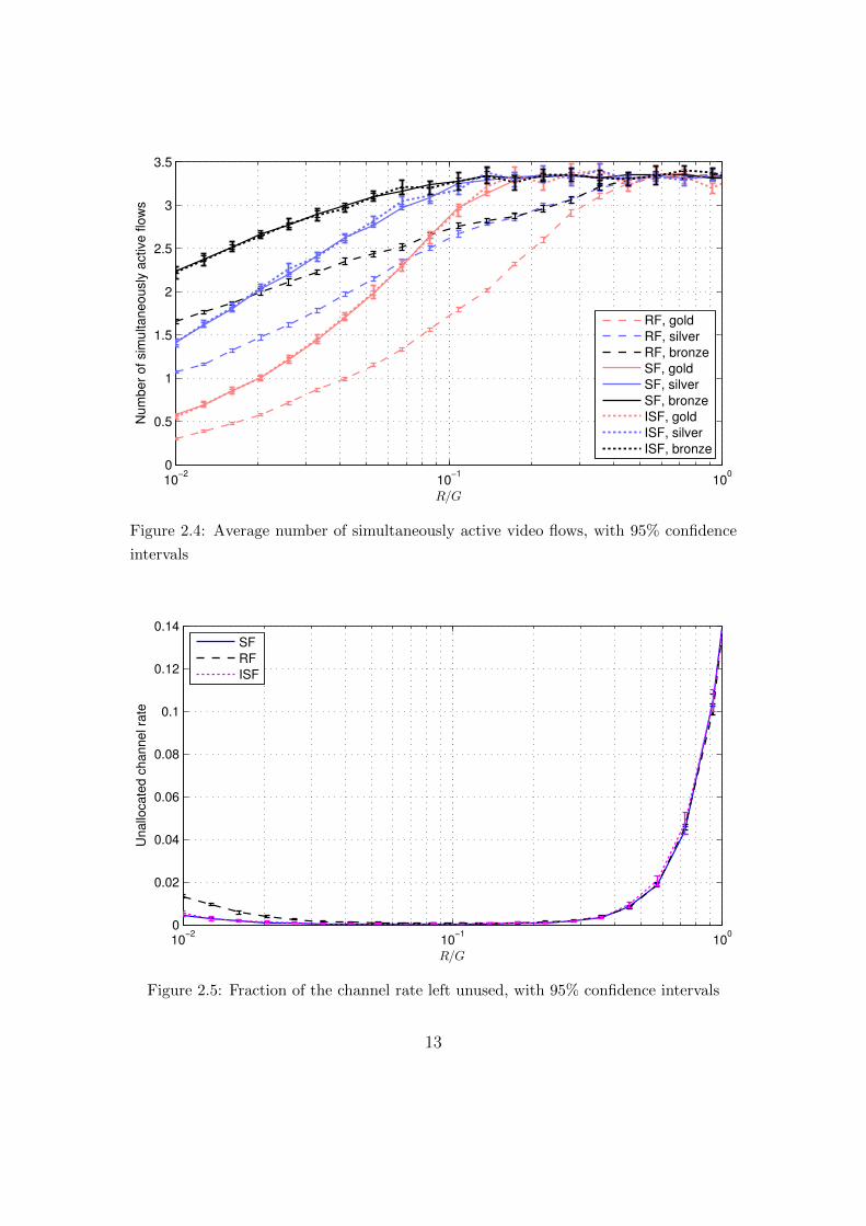
Figure 2.4: Average number of simultaneously active video flows, with 95% confidence

intervals

10−2

10−1

100

0

0.02

0.04

0.06

0.08

0.1

0.12

0.14

R/G

Un

allo

ca

ted

ch

an

ne

l ra

te

SF

RF

ISF

Figure 2.5: Fraction of the channel rate left unused, with 95% confidence intervals

13

scheme is being used. The reason of these results is revealed by the curves shown

in Figures 2.3 and 2.4, where the block probability and the number of active flows

for each quality class using the three RM algorithms are reported. We can ob-

serve, in fact, that in the considered channel rate range, SF and ISF are able to

pack more video flows in the channel and, consequently, the block probability is

smaller for SF and ISF than for RF. This is because RF does not take into account

the relationship between SSIM index and video rate, hence it cannot reduce the

quality of videos with a SSIM much greater than the class threshold in favor of

videos that do not meet the minimum QoE condition. As a consequence, the VAC

algorithm will accept more video requests with SF and ISF than with RF, though

the average quality of the accepted videos will be, on average, lower than that

achieved with RF.

To mitigate this problem, ISF tries to reduce, with respect to the SF allocation,

the rate allocated to gold flows in favor of silver and bronze flows. This allows a

great increase in SSIM values for silver and bronze video flows, at the cost of an

insignificant reduction in quality of gold flows. This is because typical RSF-SSIM

curves (Figure 2.1) are almost flat for values of RSF near 0, so that a small rate

decrease for such video flows does not impact in a significant way the video quality.

When comparing the values of average number of active flows for various classes

of videos using the same RM algorithm, it can be seen that the highest number

of flows are of bronze class, followed by silver class and then gold class, for all

RM algorithms. This is because bronze flows have lower requirements in terms

of minimum SSIM value (and so minimum bitrate), allowing them to be accepted

even when the channel is particularly crowded. Gold video flows require, instead,

higher resources, which could be not available when the channel is already used by

an high number of flows. Analogously, the probability of rejection per class shows

the same situation, where, with any of the considered algorithms, flows belonging

to the gold class are the most likely to be rejected, while bronze video flows have

14

the lowest probability of rejection. Of course, it is possible to encompass a class

downgrade mechanism to avoid blocking, but this variant has not been considered.

In Figure 2.5 the fraction of channel bandwidth that is left unused by RF, SF

and ISF is reported. All algorithms have an U-shaped behaviour as a function of

the ratio R/G. When the aggregate offered traffic for full quality videos is much

higher than the channel rate, namely R/G < 0.1, it is possible to note that the

RF leaves more unallocated capacity or, equivalently, it uses less resources than

SF and ISF. This happens because RF, considering only the nominal video rate

for resource allocation, will not decrease the rate of videos that are well above the

minimum quality threshold in order to make space for additional videos, which will

hence be blocked by the VAC algorithm despite some resources remaining unused.

For R/G > 0.1, instead, the fraction of unused capacity by all algorithms grows

quite rapidly. This happens because the channel rate is comparable with respect

to the sum of full quality rate of all active video flows, so, when the offered traffic

is lower than its average value because of the fluctuations of the video request

process, the channel resources are sufficient to transmit all the active video flows

at full quality, thus leaving some unused resources. This is also confirmed from

Figure 2.2, where we can see that, in this region, the average video quality grows

as quickly as the fraction of unallocated channel bandwidth.

As a general remark, we can see that RF manages to get better average SSIM

values with respect to SF, while, on the contrary, SF allocates videos in such a

way to allow a bigger number of simultaneously active flows with respect to RF.

ISF, instead, manages to get the overall best behaviour amongst the analyzed

algorithms, providing average SSIM values near to the ones obtained using RF,

while keeping video rejection probabilities, average number of active flows and

fraction of unallocated channel rate essentially identical to the ones obtained using

SF.

15

16

Chapter 3

Adaptive bitrate streaming

3.1 Introduction to adaptive streaming

Adaptive bitrate streaming is a technique that enables optimum multimedia stream-

ing over telecommunication networks across a wide range of devices and connection

speeds. Its main peculiarity is the ability to detect and monitor user’s available

bandwidth and CPU capacity to adapt in real-time the video flow bit rate accord-

ingly.

In particular, adaptive streaming is a method of multimedia streaming where

the source content is encoded at multiple bit rates, then each coded content is

splitted in segments with duration of a few seconds. Retrieving a manifest file,

the client can be aware of the presence of these multiple encoded versions and the

location of the various segments. Now the client is able to retrieve the segments

to playback the whole multimedia content choosing, for each temporal interval,

the segment relative to the desired quality level. This choice can be made in an

autonomous way by the client, based on available network bandwidth and on CPU

capacity of user’s device.

A key difference between streaming technologies is the type of used streaming

protocol. While in the past the most adopted solutions used protocols like RTP

17

with RTSP, nowadays adaptive streaming technologies are almost exclusively based

on HTTP. This allows to have various advantages with respect to other solutions,

in particular:

• it allows the reuse of existing server infrastructure, without the need to have

dedicated servers as in the case for RTP streaming;

• it is firewall-friendly, because with HTTP protocol the video streaming pack-

ets are generally not blocked by firewalls;

• it can exploit existing HTTP cache infrastructure to offer video segments

from a nearer location to the user with respect to the original server, enabling

faster video delivery.

3.2 Introduction to MPEG-DASH

MPEG-DASH (Dynamic Adaptive Streaming over HTTP) [5] is an ISO standard

developed by the Motion Picture Experts Group (MPEG) that defines an adaptive

bitrate streaming technique based on HTTP.

DASH development started in 2010, evolving into a Draft International Stan-

dard in January 2011 and an International Standard in November 2011. The

MPEG-DASH standard, first published in April 2012 as ISO/IEC 23009-1, has

been updated on July 2013, incorporating some amendments and corrigenda.

MPEG-DASH is the first HTTP-based adaptive streaming solution that arose

at the level of international standard. It was preceded by similar, but proprietary,

adaptive streaming technologies, like Adobe’s HTTP Dynamic Streaming, Ap-

ple’s HTTP Live Streaming [9] and Microsoft’s Smooth Streaming. The objective

for MPEG-DASH was to replace those technologies by incorporating their strong

points into a widely implemented and vendor-independent standard, in order to

enable the use of a single technology for multimedia streaming on all platforms.

To reach this objective, the standardization group worked together with the most

18

important stakeholders, like Adobe, Apple, Microsoft, Netflix and Qualcomm, and

with other standardization bodies, in particular with 3GPP, that was developing

a similar technology, called Adaptive HTTP Streaming (AHS) [10].

Nowadays the standard is implemented in various products and gained traction

as the only available technology allowing adaptive bitrate streaming on devices

from different vendors.

3.3 DASH data model

MPEG-DASH defines a media content delivery model where the control is pri-

marily client-side. In fact, clients may request data, using HTTP protocol, from

standard web servers that have no DASH-specific capabilities. Because of that,

the DASH standard focalizes on data formats used in data exchanges and not on

client and server procedures.

The set of deliverable encoded versions of media content, along with their

description, forms a Media Presentation. A DASH Media Presentation is described

by an XML manifest file called Media Presentation Description (MPD) [5].

Media content is composed by one or more contiguous periods in time. These

periods could represent parts or episodes of a main program, interleaved with

inserted advertisement periods. The set of the available coded versions of me-

dia content must be consistent throughout a period, i.e., the available languages,

subtitles, bitrates, etc. can not change within a period.

In a period, material is divided in adaptation sets. An adaptation set represents

a set of coded version of a media component. For example, there could be an

adaptation set for the main video component and a separate one for the main audio

component. Other components, like subtitles or other audio tracks, could have a

dedicate adaptation set each. Those media components could also be provided in

multiplexed form. In this case, interchangeable versions of the multiplex may be

described with a single adaptation set. An example for this case is an adaptation

19

Media Presentation Description (MPD)

Period

Adaptation Set

Representation

Segment

Segment

Segment

Representation

Segment

Segment

Segment

Representation

Segment

Segment

Segment

Adaptation Set

Period

Figure 3.1: DASH data model

20

set containing both the main audio and main video for a period, with additional

components being provided in additional adaptation sets.

An adaptation set contains a set of representations. A representation describes

a deliverable encoded version of one or multiple media content components. Each

representation in an adaptation set is sufficient to render the contained media

components, but, grouping together several representations in a single adaptation

set, the Media Presentation author states that those representations represent

perceptually equivalent contents. This means that clients can dynamically swicth

between representations in an adaptation set in order to adapt to network condi-

tions or other factors. Switching refers to the presentation of decoded data of one

representation up to a certain time instant, and the presentation of decoded data

of another representation from that instant onwards. If both representations are

included in the same adaptation set, and the client switches properly, the media

playout is perceived seamless across the switch.

Within a representation, the content may be divided in time into segments. In

order to access a segment, an URL is provided for each segment.

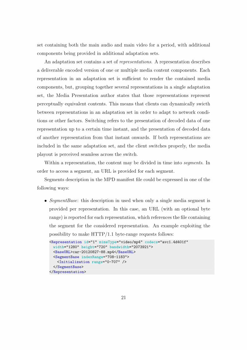
Segments description in the MPD manifest file could be expressed in one of the

following ways:

• SegmentBase: this description in used when only a single media segment is

provided per representation. In this case, an URL (with an optional byte

range) is reported for each representation, which references the file containing

the segment for the considered representation. An example exploiting the

possibility to make HTTP/1.1 byte-range requests follows:

<Representation id="1" mimeType="video/mp4" codecs="avc1.4d401f"

width="1280" height="720" bandwidth="2073921">

<BaseURL>car-20120827-88.mp4</BaseURL>

<SegmentBase indexRange="708-1183">

<Initialization range="0-707" />

</SegmentBase>

</Representation>

21

• SegmentList : in this case the description of each representation includes a

list of segment URLs, one for each segment of the considered representa-

tion. Each segment URL is composed by a file location and, optionally, a

byte range, allowing to make byte-range requests according to HTTP/1.1

specification. A self-explanatory example for this case follows:

<Representation id="1" mimeType="video/mp4" codecs="avc1.640016"


<BaseURL>akiyo0_dashinit.mp4</BaseURL>

<SegmentList timescale="1200000" duration="5952000">

<Initialization range="0-865"/>

<SegmentURL mediaRange="866-4205261" indexRange="866-969"/>



</SegmentList>

</Representation>

• SegmentTemplate: in this case, the list of segment URLs is expressed by a

template and some replacement rules that allows to swap special identifiers

with appropriate dynamic values assigned to segments. The simplest case

is when the template is made by a fixed part and an index that assumes

increasing values for successive segments. In this way it’s possible to use

DASH technology for streaming of live media content, where segments are

delivered to clients while successive ones are still being generated, making

impossible the creation of a segment URLs list beforehand. A simple example

of this case, where $Number$ is the placeholder for the segment number, could

be:

<Representation id="1" mimeType="video/mp4" codecs="avc1.640016"


<SegmentTemplate timescale="1200000" media="seg_bowing0$Number$.m4s"

startNumber="1" duration="2304000" initialization="seg_bowing0init.mp4"/>

</Representation>

22

<?xml version="1.0"?>

<MPD xmlns="urn:mpeg:dash:schema:mpd:2011" minBufferTime="PT1.500000S" type="static"

mediaPresentationDuration="PT0H0M12.00S" profiles="urn:mpeg:dash:profile:full:2011">

<ProgramInformation> <Title>akiyo0_dash.mpd</Title> </ProgramInformation>

<Period duration="PT0H0M12.00S">

<AdaptationSet segmentAlignment="true" maxWidth="352"

maxHeight="288" maxFrameRate="25" par="352:288">

<Representation id="1" mimeType="video/mp4" codecs="avc1.640016" width="352"

height="288" frameRate="25" sar="1:1" startWithSAP="1" bandwidth="6772590">







</SegmentList>

</Representation>









</SegmentList>

</Representation>









</SegmentList>

</Representation>

</AdaptationSet>

</Period>

</MPD>

Figure 3.2: Example of an MPD manifest file

23

3.4 Typical DASH client operation

The typical DASH client procedure to retrieve and render a media stream consists

of the following steps:

1. the client retrieves the MPD manifest file from the server and parses it to be

aware of all available media components and their representations;

2. the retrieval of the media starts with the download of first segments relative

to the desired media components. Usually, the low bitrate version of first

segments are chosen, because of the unknown network conditions. In this

way, it is also possible to get a faster start of video playout. MPD manifest

may also indicate the necessity to retrieve an initialization segment, contain-

ing information needed to initialize the media engines for enabling playout

of the media segments. If this is not the case, segments are said to be self-

initializing, because each of them contains all the necessary information for

its decoding.

3. The client estimates network conditions from metrics calculated from previ-

ous segments download. These metrics will be helpful in chosing the bitrate

of the next media segments to retrieve.

4. Successive segments are retrieved using the metrics calculated in the preced-

ing step. In case of not self-initializing segments, if the new segment belongs

to a different Representation with respect to the previous one, the initializa-

tion segment for that Representation must be retrieved in order to correctly

decode the new segment.

5. Steps 3-4 are repeated until all desired media components are completely

retrieved.

24

3.5 Additional DASH features

DASH technology provides additional features, such as:

• being codec independent, it works with H.264, WebM and other codecs,

allowing this technology to be future-proof and adaptable to new codec that

will be developed;

• the possibility to support all encryption schemes and DRM techniques spec-

ified in ISO/IEC 23001-7 standard enables its use in commercial streaming

services;

• it allows for dynamic ads insertion, useful again for commercial streaming

services;

• it entails special features to support live streaming, like the possibility to

fragment the MPD manifest and download each fragment separately (used

to update the manifest with new information that become available after the

stream start).

25

26

Chapter 4

Resource Management proxy

In this work, we propose the use of a transparent Resource Management proxy

between the clients and the video server. The purpose of the proxy is to intercept

segment requests from clients and redirect them to enforce a resource allocation

according to one of the algorithms seen in Section 2.2.1. The use of a transparent

proxy allows us to not be tied to the support of a dedicated protocol by the clients

and the server. The proxy server is based on mitmproxy [11], an SSL-capable

man-in-the-middle proxy for HTTP. This software is able to act as a transparent

proxy, thus not requiring any special client or server configuration. In fact, the key

property of the RM proxy is to be completely transparent to both the client and

the video server. Software of the RM proxy has been written using Python and

C, through the use of Cython compiler [12], and employs the scientific libraries

NumPy [13] and SciPy [14] to avoid any delay in communications introduced by

the proxy processing.

The RM proxy has to be placed between the DASH clients and the HTTP

servers, in such a way to intercept every request from clients to servers and every

related response. Also, the proxy must know the rate of the channel bottleneck

between client and server.

27

The operations that the proxy performs are different based on the type of inter-

cepted message. In particular, there are three cases: an MPD request from a client,

a media request from a client, a media response from the server. Other messages

are simply forwarded without further processing. Now the three aforementioned

cases will be discussed.

MPD request from a client

In this case a client requests an MPD manifest from the server. The proxy considers

this request as the start of a new flow, so it retrieves itself the manifest file, parses

it and saves the information contained in it, in particular the set of available

representations, along with their bandwidth requirement, and the set of segment

URLs for each representation. Note that the bitrate of full quality version of

the video can also be obtained from these information, picking the maximum

bitrate between all representations. Information allowing the identification of the

requesting client, like its IP address, are also also stored and associated with this

video flow.

Then, the proxy must obtain the polynomial coefficients indicating the relation-

ship between SSIM index and Rate Scaling Factor. As mentioned in the previous

chapters, these coefficients could be obtained directly by the server or estimated

through a machine learning approach [8]. In the first case, an appropriate server

request must be sent and the response must be parsed to retrieve the coefficients.

In the second case, the coefficients have to be estimated with the use of a video

segment. There are two possible options to retrieve the segment:

• Immediately retrieve a video segment from the server. The drawback here

comes from the need, for the server, to support a dedicated protocol. The

advantage is that the coefficients are immediately available for use in the

optimization routine.

28

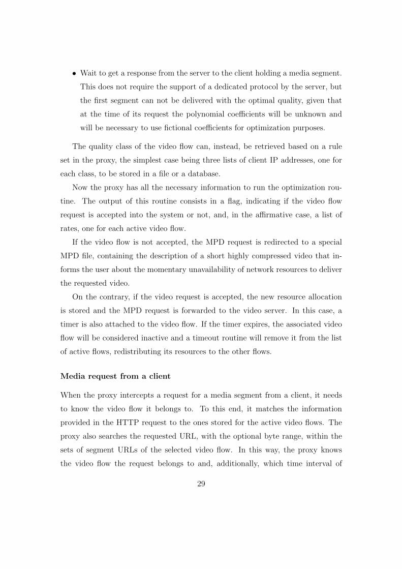
• Wait to get a response from the server to the client holding a media segment.

This does not require the support of a dedicated protocol by the server, but

the first segment can not be delivered with the optimal quality, given that

at the time of its request the polynomial coefficients will be unknown and

will be necessary to use fictional coefficients for optimization purposes.

The quality class of the video flow can, instead, be retrieved based on a rule

set in the proxy, the simplest case being three lists of client IP addresses, one for

each class, to be stored in a file or a database.

Now the proxy has all the necessary information to run the optimization rou-

tine. The output of this routine consists in a flag, indicating if the video flow

request is accepted into the system or not, and, in the affirmative case, a list of

rates, one for each active video flow.

If the video flow is not accepted, the MPD request is redirected to a special

MPD file, containing the description of a short highly compressed video that in-

forms the user about the momentary unavailability of network resources to deliver

the requested video.

On the contrary, if the video request is accepted, the new resource allocation

is stored and the MPD request is forwarded to the video server. In this case, a

timer is also attached to the video flow. If the timer expires, the associated video

flow will be considered inactive and a timeout routine will remove it from the list

of active flows, redistributing its resources to the other flows.

Media request from a client

When the proxy intercepts a request for a media segment from a client, it needs

to know the video flow it belongs to. To this end, it matches the information

provided in the HTTP request to the ones stored for the active video flows. The

proxy also searches the requested URL, with the optional byte range, within the

sets of segment URLs of the selected video flow. In this way, the proxy knows

the video flow the request belongs to and, additionally, which time interval of

29

the video clip the client requested. The proxy is then able to build up a pair

formed by a representation index and a segment index, where the segment index

indicates which time interval the client requested, as retrieved in the previous step,

while the representation index is relative to the representation that best matches

the optimum bitrate allocation for the given flow. There are two possible ways

to choose this optimum representation: the first is to choose the representation

with the most similar bandwidth to the optimal one, the second is to choose the

representation with the highest bandwidth between the ones with a bandwidth

smaller than the optimum. In Section 5.1 the two options will be compared, coming

to the conclusion that, even if the first option allows a better channel exploitation,

it will cause, with a significant probability, the sum of bitrates allocated to video

flows to exceed the available channel rate, causing playout buffer underflows and,

consequently, video freezing phenomena at clients. With the appropriate indices

pair set up, the proxy is then able to search, through the list of segment URLs, the

URL where the request needs to be redirected. The last step, before the request

forwarding, is to check if the request is relative to a last segment of the video, in

one of its representation. If this is the case, the flow is marked for removal after the

reponse will be transmitted. In every case, the timer associated to the video flow

is reset. The headers of the request are then rewritten to apply the redirection to

the correct segment. As a last step, the request is forwarded to the media server.

Media response from the server

When the proxy receives a media response from the server, it checks if the associ-

ated flow is marked for removal. If it is, it forwards the request to the client and

then, at the end of the transmission, it removes the flow from the list of active ones

and runs the RM algorithm to redistribute the freed resources to the other active

flows. It is worth noting that the VAC algorithm needs not to be invoked, because

each video will get equal or more resources than it had before, consequently its

30

quality level can not decrease. If the flow is not marked for removal, the media

response is simply forwarded to the client.

31

32

Chapter 5

Experimental results

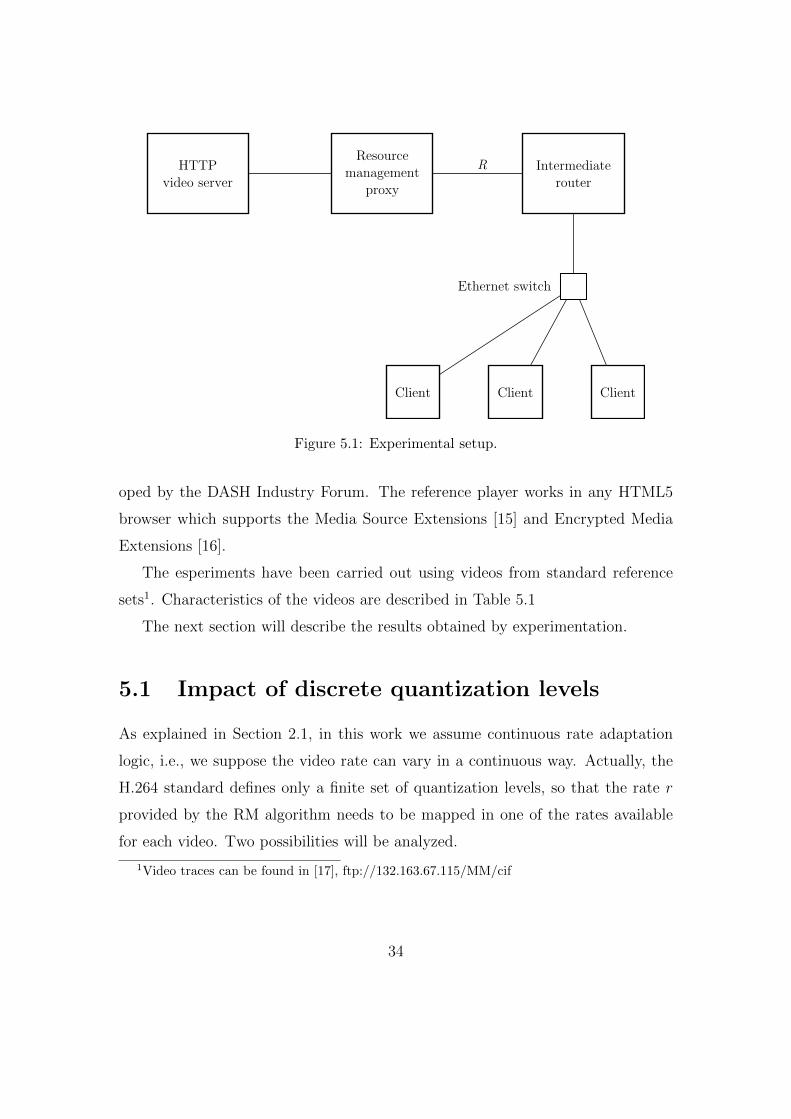
A number of experiments have been carried on to evaluate the RM proxy perfor-

mance. The setting (Figure 5.1) is composed by a video server connected through

a high speed link to the RM proxy, which is, in turn, connected to a router through

a low speed link of rate R, which is the network bottleneck. The router is then con-

nected, through a switch, to the clients. In these experiments all links uses IEEE

802.3 100BASE-TX standard technology with a maximum rate of 100 Mbit/s.

The rate of the bottleneck has been throttled using the netem network emulator

available in the Linux kernel. The server runs Debian 7.6 Linux distribution and

uses Apache HTTP server to provide the functionality of a DASH video server.

The RM proxy runs on Ubuntu 14.04 LTS Linux distribution with Python 2.6,

while the router and the clients all run Debian 7.6 Linux distribution. Clients use

the Google Chrome 37 browser to run the DASH Reference Player dash.js, devel-

Video Length Full quality bitrate

paris 42.6 s 12041 kbit/scoastguard 12 s 14910 kbit/sfootball 3.6 s 14296 kbit/sbowing 12 s 10060 kbit/s

Table 5.1: Video characteristics

33

HTTP

video server

Resource

management

proxy

Intermediate

router

Ethernet switch

Client Client Client

R

Figure 5.1: Experimental setup.

oped by the DASH Industry Forum. The reference player works in any HTML5

browser which supports the Media Source Extensions [15] and Encrypted Media

Extensions [16].

The esperiments have been carried out using videos from standard reference

sets1. Characteristics of the videos are described in Table 5.1

The next section will describe the results obtained by experimentation.

5.1 Impact of discrete quantization levels

As explained in Section 2.1, in this work we assume continuous rate adaptation

logic, i.e., we suppose the video rate can vary in a continuous way. Actually, the

H.264 standard defines only a finite set of quantization levels, so that the rate r

provided by the RM algorithm needs to be mapped in one of the rates available

for each video. Two possibilities will be analyzed.

1Video traces can be found in [17], ftp://132.163.67.115/MM/cif

34

0

2

4

6

8

10

12

14

TH FLOOR NEAR TH FLOOR NEAR

rate

(M

bit

/s)

pariscoastguard

football

3 flows2 flows

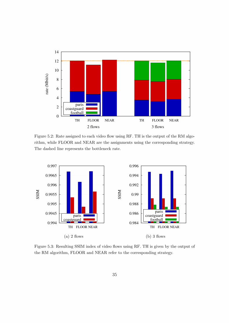
Figure 5.2: Rate assigned to each video flow using RF. TH is the output of the RM algo-

rithm, while FLOOR and NEAR are the assignments using the corresponding strategy.

The dashed line represents the bottleneck rate.

0.994

0.9945

0.995

0.9955

0.996

0.9965

0.997

TH FLOOR NEAR

SS

IM

pariscoastguard

(a) 2 flows

0.984

0.986

0.988

0.99

0.992

0.994

0.996

TH FLOOR NEAR

SS

IM

pariscoastguard

football

(b) 3 flows

Figure 5.3: Resulting SSIM index of video flows using RF. TH is given by the output of

the RM algorithm, FLOOR and NEAR refer to the corresponding strategy.

35

0

2

4

6

8

10

12

14

TH FLOOR NEAR TH FLOOR NEAR

rate

(M

bit

/s)

pariscoastguard

football

3 flows2 flows

Figure 5.4: Rate assigned to each video flow using RF. TH is the output of the RM algo-

rithm, while FLOOR and NEAR are the assignments using the corresponding strategy.

The dashed line represents the bottleneck rate.

0.995

0.9955

0.996

0.9965

0.997

TH FLOOR NEAR

SS

IM

pariscoastguard

(a) 2 flows

0.99

0.9902

0.9904

0.9906

0.9908

0.991

0.9912

0.9914

TH FLOORNEAR

SS

IM

pariscoastguard

football

(b) 3 flows

Figure 5.5: Resulting SSIM index of video flows using SF. TH is given by the output of

the RM algorithm, FLOOR and NEAR refer to the corresponding strategy.

36

VideoRF SF

FLOOR NEAR FLOOR NEAR

paris 0 (0%) 0 (0%) 0 (0%) 0 (0%)coastguard 0 (0%) 0 (0%) 0 (0%) 0 (0%)football 0 (0%) 0.325 (9.03%) 0 (0%) 0.063 (1.75%)

Table 5.2: Freezing time in seconds for each video flow (values in brackets indicate the

freezing time as fraction of video length).

The first, called FLOOR, consists in choosing the maximum available rate that

is smaller than or equal to the given rate r. Formally, if the set of available rates

is denoted r = {r1, r2, . . .}, the chosen rate is

ri = max{rk ∈ r | rk ≤ r}. (5.1)

The second policy, called NEAR, simply chooses the available rate that is the

closest to the given rate r. Formally, the chosen rate is given by

ri = argminrk∈r

{|rk − r|}. (5.2)

To evaluate the impact of the chosen strategy on the proxy performance, an

experiment involving three clients has been set up. The first client sends the

request for the streaming of video paris, which will be immediately activated,

then, 20 seconds later, the second client starts playing the coastguard video, while

video paris is still being streamed. Finally, after other 5 seconds, the football video

starts playing, for a total of three simultaneously active videos. All video flows

have been assigned class bronze. Therefore, SF and ISF perform in the same way,

so that only results obtained using SF are shown. The rate of the bottleneck is

set at R = 12041 kbit/s, which corresponds to the rate of the full quality version

of paris video.

37

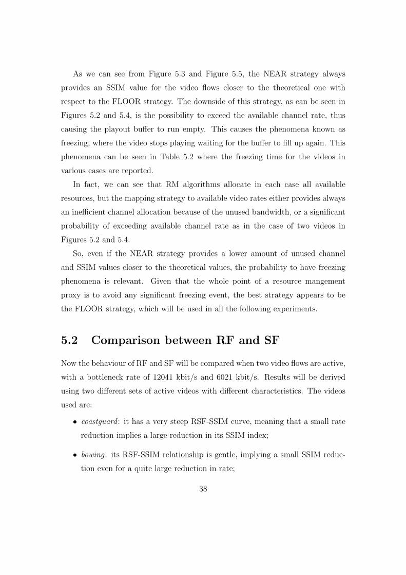
As we can see from Figure 5.3 and Figure 5.5, the NEAR strategy always

provides an SSIM value for the video flows closer to the theoretical one with

respect to the FLOOR strategy. The downside of this strategy, as can be seen in

Figures 5.2 and 5.4, is the possibility to exceed the available channel rate, thus

causing the playout buffer to run empty. This causes the phenomena known as

freezing, where the video stops playing waiting for the buffer to fill up again. This

phenomena can be seen in Table 5.2 where the freezing time for the videos in

various cases are reported.

In fact, we can see that RM algorithms allocate in each case all available

resources, but the mapping strategy to available video rates either provides always

an inefficient channel allocation because of the unused bandwidth, or a significant

probability of exceeding available channel rate as in the case of two videos in

Figures 5.2 and 5.4.

So, even if the NEAR strategy provides a lower amount of unused channel

and SSIM values closer to the theoretical values, the probability to have freezing

phenomena is relevant. Given that the whole point of a resource mangement

proxy is to avoid any significant freezing event, the best strategy appears to be

the FLOOR strategy, which will be used in all the following experiments.

5.2 Comparison between RF and SF

Now the behaviour of RF and SF will be compared when two video flows are active,

with a bottleneck rate of 12041 kbit/s and 6021 kbit/s. Results will be derived

using two different sets of active videos with different characteristics. The videos

used are:

• coastguard : it has a very steep RSF-SSIM curve, meaning that a small rate

reduction implies a large reduction in its SSIM index;

• bowing : its RSF-SSIM relationship is gentle, implying a small SSIM reduc-

tion even for a quite large reduction in rate;

38

0

2

4

6

8

10

12

RF SF RF SF

rate

(M

bit

/s)

paris pariscoastguard bowing

pariscoastguard

bowing

(a) Video rates, the dashed line represents

the bottleneck rate

0.995

0.9955

0.996

0.9965

0.997

0.9975

0.998

RF SF RF SF

SS

IM


pariscoastguard

bowing

(b) SSIM index

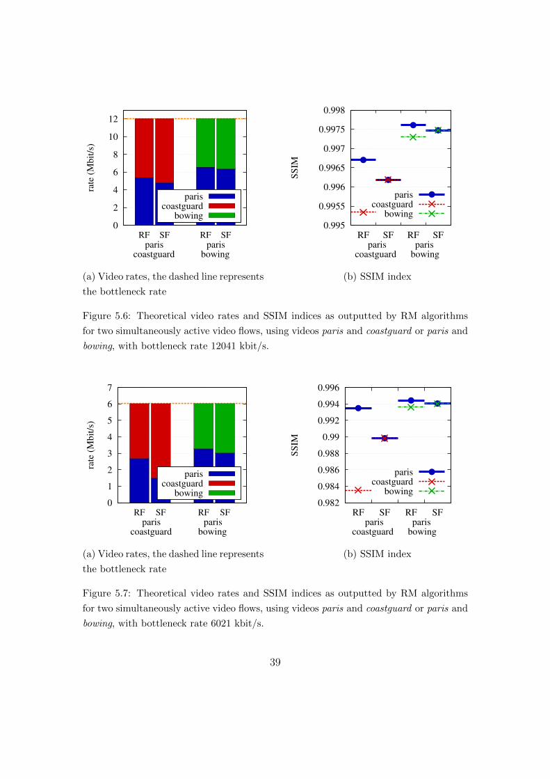
Figure 5.6: Theoretical video rates and SSIM indices as outputted by RM algorithms

for two simultaneously active video flows, using videos paris and coastguard or paris and

bowing, with bottleneck rate 12041 kbit/s.

0

1

2

3

4

5

6

7

RF SF RF SF

rate

(M

bit

/s)


pariscoastguard

bowing


the bottleneck rate

0.982

0.984

0.986

0.988

0.99

0.992

0.994

0.996

RF SF RF SF

SS

IM


pariscoastguard

bowing

(b) SSIM index

Figure 5.7: Theoretical video rates and SSIM indices as outputted by RM algorithms

for two simultaneously active video flows, using videos paris and coastguard or paris and


39

0

2

4

6

8

10

12

RF SF RF SF

rate

(M

bit

/s)


pariscoastguard

bowing


the bottleneck rate

0.9945

0.995

0.9955

0.996

0.9965

0.997

0.9975

RF SF RF SF

SS

IM


pariscoastguard

bowing

(b) SSIM index

Figure 5.8: Resulting video rates and SSIM indices for two simultaneously active video

flows with discrete quantization levels, using videos paris and coastguard or paris and


0

1

2

3

4

5

6

7

RF SF RF SF

rate

(M

bit

/s)


pariscoastguard

bowing


the bottleneck rate

0.982

0.984

0.986

0.988

0.99

0.992

0.994

0.996

RF SF RF SF

SS

IM


pariscoastguard

bowing

(b) SSIM index

Figure 5.9: Resulting video rates and SSIM indices for two simultaneously active video

flows with discrete quantization levels, using videos paris and coastguard or paris and


40

• paris : its RSF-SSIM curve behaviour is halfway between those of the other

two videos.

As we can see from Figure 5.6a, when the active videos are composed by the

couple paris and coastguard, the coastguard flow gets assigned by the RF a higher

rate than that assigned to the paris video, because the full quality rate of coast-

guard is bigger than the one of paris video. Nevertheless, the SSIM value of

coastguard video is still way lower than the one for paris video, as we can see in

Figure 5.6b. To get equal SSIM values for both videos, SF allocates even more rate

to the coastguard video, allowing them to reach an SSIM value of 0.996182, which

is slightly larger than the average between the SSIM indices of the two videos for

the RF case, equal to 0.996021. Since all videos belong to the same class, ISF and

SF provide identical results.

When the active videos are paris and bowing, instead, RF assigns a lower rate

to the bowing video than to paris video. But, in this way, paris video still gets

higher SSIM, so that to reach the same SSIM value for both videos, SF allocates

to bowing video an even higher rate than that allocated by RF, while reducing the

rate of paris video. With these videos the SF provides an average SSIM equal to

0.997473, which is again slightly larger than the one obtained using RF, where the

average SSIM is 0.997453.

It is important to note that using SF, the gap between the rates of paris and

coastguard videos is wider than that given by RF. With videos paris and bowing,

instead, the SF provides a more even rate allocation between the two videos with

respect to the allocation calculated by RF. This indicates that, even if the feature

used by RF to calculate the optimal allocation (the full quality rate of videos)

is correlated to the quality-rate curve, this characteristic does not contain all the

information needed to obtain a real fairness on quality, like the one reached by SF.

Results with the bottleneck rate of 6021 kbit/s (Figure 5.7) confirm what al-

ready observed in the previous paragraphs, showing that these results do not

depend on the bottleneck rate.

41

Plots built using the real values of rate and SSIM for streamed video (instead

of the theoretical results given by the RM algorithms) show that small differences

in rate allocation between the algorithms, as in the case of videos paris and bowing

in Figure 5.6a, often do not make practical difference (Figure 5.8a), because they

are evened out by the application of discrete quantization levels. Bigger differences

in rate allocation between RF and SF, instead, affect the real flow rates and SSIM

values, like in Figure 5.9. Another thing to note analyzing the real SSIM values

of video flows (Figures 5.8b and 5.9b) is that, obviously, exact SSIM fairness can

not be reached even using SF, but, in this regard, SF is still much more capable

of providing quality fairness with respect to RF.

5.3 Comparison between classless and classfull

RM algorithms

One of the most important part of RM algorithms is related to the management

of quality classes. In fact, this feature is one of the most important selling points

of the resource amangement proxy, because clients can not manage quality classes

and, even if they could, the class assigned to a user could be overridden by client,

which is under the user’s control.

With this experiment, we will compare rate allocation and SSIM values ob-

tained by appointing different classes to flows using both SF and ISF. As already

stated, these two algorithms perform equally in the case of single class video flows.

Videos used are the usual paris, coastguard and football. Experiments with a sin-

gle class have been conducted appointing bronze class to all flows. In experiments

using multiple classes, instead, video paris has been assigned bronze class, video

coastguard has been assigned silver class and video football has been assigned gold

class.

As we can see from Figure 5.5, using SF with a single class for all video flows

leads to all flows having the same SSIM value, thus reaching a perfect SSIM fair-

42

0.92

0.93

0.94

0.95

0.96

0.97

0.98

0.99

1

SF ISF

SS

IM

pariscoastguard

(a) 2 flows

0.86

0.88

0.9

0.92

0.94

0.96

0.98

1

SF ISFS

SIM

pariscoastguard

football

(b) 3 flows

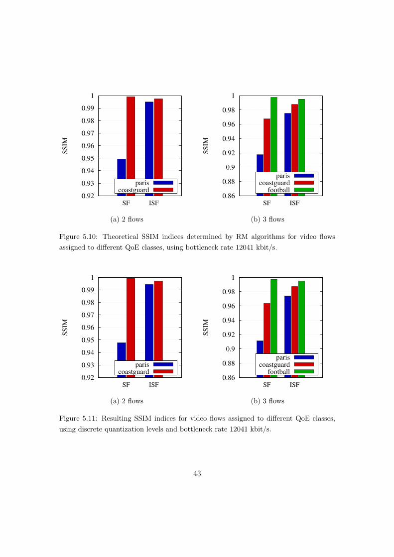
Figure 5.10: Theoretical SSIM indices determined by RM algorithms for video flows

assigned to different QoE classes, using bottleneck rate 12041 kbit/s.

0.92

0.93

0.94

0.95

0.96

0.97

0.98

0.99

1

SF ISF

SS

IM

pariscoastguard

(a) 2 flows

0.86

0.88

0.9

0.92

0.94

0.96

0.98

1

SF ISF

SS

IM

pariscoastguard

football

(b) 3 flows

Figure 5.11: Resulting SSIM indices for video flows assigned to different QoE classes,

using discrete quantization levels and bottleneck rate 12041 kbit/s.

43

ness, as already stated before. When analyzing results obtained using SF with

multiple classes (Figure 5.10), instead, all flows have an SSIM value equal to the

sum of the baseline SSIM for each class and an increment α in common between

all classes. This result is in accordance with the theoretical explanation of SF

in Section 2.2.1. In particular, the increment is α = 0.049164 when two videos

are active and α = 0.017349 when three videos are active. With respect to the

classless case, there is now an increase in SSIM value for coastguard and football

videos, to the detriment of paris video, which gets a low SSIM value because of

its low quality class.

With respect to the SF classfull case, the ISF classfull scenario has an increment

in SSIM values for low quality classes, with a compensating decrement for high

quality classes. In particular, in the case of two videos, paris has an increment of

0.046, while coastguard has a decrement of just 0.002 in SSIM value. In case of

three active flows, paris video has an increment of 0.058 and coastguard gains 0.020

in SSIM value, while football is affected by a SSIM decrement of just 0.002. This

confirms the validity of the reasoning behind ISF: a minimal loss on SSIM for gold

flows allows for big quality gains in the other classes. This is because RSF-SSIM

graph (Figure 2.1) is almost flat for RSF near 0, so that a rate decrement in that

region does not affect significantly the SSIM value.

Both theoretical and experimental results from RM algorithms (Figures 5.10

and 5.11) show the same behaviour concerning this aspect, so that the effects of

discrete quantization levels are not significant when comparing these algorithms.

5.4 Comparison between RM proxy and client

adaptation logic performance

The objective of this experiment is to find out if the use of RM proxy can actually

provide better performance than the use of client adaptation logic alone. The

experiment consists in the successive activation of videos paris, coastguard and

44

0

2

4

6

8

10

12

14

0 5 10 15 20 25 30 35 40

rate

(M

bit

/s)

time (s)

paris (ISF)

paris (CAL)

coastguard (ISF)

coastguard (CAL)

football (ISF)

football (CAL)

(a) Rate values

0.88

0.9

0.92

0.94

0.96

0.98

1

0 5 10 15 20 25 30 35 40

SS

IM

time (s)

paris (ISF)

coastguard (ISF)

football (ISF)

paris (CAL)

coastguard (CAL)

football (CAL)

(b) SSIM values

Figure 5.12: Time evolution of video flows rate and SSIM with ISF and client adaptation

logic (CAL).

45

Video SF CAL

paris 0 (0%) 0 (0%)coastguard 0 (0%) 0 (0%)football 0 (0%) 2.385 (66.25%)

Table 5.3: Freezing time in seconds for each video flow, values between parenthesis

indicate the freezing time as fraction of video length.

football. Results in terms of video rates, SSIM indices and freezing time have been

collected using both the adaptation logic integrated in the clients (indicated with

CAL in the following) and the use of RM proxy. Given that, without the proxy,

clients can not be divided in quality classes, all video flows have been assigned to

quality class bronze when using the RM proxy, to get results comparable to the

ones obtained with the use of client adaptation logic. The RM algorithm used in

the proxy is ISF (it is to note that SF performs as ISF when a single class is used

for all video flows).

In Figures 5.12a and 5.12b we can see the rates and SSIM indices for the video

flows over time. The first thing to note is the oscillatory behaviour of rate and

SSIM values obtained using the client adaptation logic alone. This is because

the clients do not know the bottleneck rate, thus they have to start the play-

out with the lowest quality version of the video and then try to get progressively

better quality segments until the segment download time becomes too high and

they have to resort to a lower quality representation. The first problem with this

approach is that the client can not provide a high quality vision from the very

beginning of the video, as RM proxy allows instead. The second problem appears

when another video starts playing: immediately after this event, in fact, clients of

the already active flows keep downloading a high rate version of the videos, using

more channel resources than what available, thus resulting in freezing events with

high probability. In these occasions, the playout buffer role is really important,

because it also needs to hide the channel congestion other than the usual jitter

problems. When the clients find a congested network, they all resort to an ex-

46

tremely low quality version of the videos at first, trying to progressively increase

the flow rate over time. This behaviour causes the spiky rate and SSIM evolution

in time, visible in Figure 5.12a. This brings the client adaptation logic to incurr in

significant freezing events, summarized in Table 5.3, and yields significantly lower

video quality than using the RM proxy. The consequence of this spiky behaviour

is the alternate reproduction of medium-high quality segments and low quality

segments, which worsens the perceived quality even more. In fact, the continuous

variation of the video quality makes much more evident the image degradation

than a smooth playout with relatively low but constant quality.

The drawback of using the RM proxy is the need to know the available band-

width across the network bottleneck. If this bandwidth is not reserved for video

flows with other mechanisms, like diffserv, it must be estimated, giving the same

problems as those experienced by the client adaptation logic. However, in this case

the competing traffic does not include other video flows, which are demanding in

terms of bandwidth, but only less bandwidth hungry transmissions, which make

the above mentioned problems much less serious.

47

48

Chapter 6

Conclusions

In this thesis, different Resource Management algorithms have been described and

compared via simulations. Then, these algorithms have been used to build a

Resource Management proxy, which allocates channel resources in a QoE-aware

manner. The RM algorithms analyzed are: Rate Fairness, which assigns the rate

to each video flow in a QoE-agnostic way, SSIM Fairness, which allocates resources

such that all video flows get an SSIM value equal to their class threshold incre-

mented by a factor equal for all flows, and Improved SSIM Fairness, which exploits

the RSF-SSIM curves behaviour to improve SF performance.

From simulative results, ISF appeared to be the clear winner, enabling the

video flows to reach high SSIM values while accepting a high number of requests.

Experimentations with the RM proxy proved that the use of the proxy is able

to drastically improve the quality of video flows with respect to the use of client

adaptation logic alone, while avoiding freezing phenomena. Again, the use of ISF

proved to perform really well both in classless and classfull cases. In particular,

with this algorithm, the use of classes proved to be a viable way to provide different

QoE to different users, without penalizing too much users belonging to low QoE

classes.

49

Summing up, the use of RM proxy is particularly effective in increasing the

user experience regarding video playout, and, with the growing adoption of DASH

technology, this technique is also suitable for large scale implementation.

50

Bibliography

[1] CISCO. The Zettabyte Era: Trends and Analysis. White paper, June 2014.

[2] Dong-Hoon Shin, D. Moses, M. Venkatachalam, and S. Bagchi. Distributed

mobility management for efficient video delivery over all-IP mobile networks:

Competing approaches. IEEE Network, 27(2):28–33, March 2013.

[3] Zhou Wang, AC. Bovik, H.R. Sheikh, and E.P. Simoncelli. Image quality

assessment: from error visibility to structural similarity. IEEE Trans. Image

Processing, 13(4):600–612, April 2004.

[4] Daniele Munaretto, Daniel Zucchetto, Andrea Zanella, and Michele Zorzi.

Data-driven QoE optimization techniques for multi-user wireless networks.

In 2015 International Conference on Computing, Networking and Communi-

cations, Invited Position Papers (ICNC’15 Invited), Anaheim, USA, February

2015.

[5] Dynamic adaptive streaming over HTTP (DASH) — Part 1: Media presen-

tation description and segment formats. ISO/IEC 23009-1:2014 standard.

[6] Advanced video coding for generic audiovisual services. ITU-T Rec. H.264 &

ISO/IEC 14496-10 AVC standard.

[7] Marco Zanforlin, Daniele Munaretto, Andrea Zanella, and Michele Zorzi.

SSIM-based video admission control and resource allocation algorithms. In

51

Proceedings of the WiOpt workshop “Wireless Video Performance” (WiVid

2014), May 2014.

[8] Alberto Testolin, Marco Zanforlin, Michele De Filippo De Grazia, Daniele

Munaretto, Andrea Zanella, Marco Zorzi, and Michele Zorzi. A machine

learning approach to QoE-based video admission control and resource alloca-

tion in wireless systems. In 13th Annual Mediterranean Ad Hoc Networking

Workshop (MED-HOC-NET), pages 31–38, June 2014.

[9] R.P. Pantos and W.M. May. HTTP Live Stream-

ing. IETF Internet Draft. https://tools.ietf.org/html/

draft-pantos-http-live-streaming-13.

[10] Transparent end-to-end Packet-switched Streaming Service (PSS); Progres-

sive Download and Dynamic Adaptive Streaming over HTTP (3GP-DASH).

3GPP TS 26.247.

[11] mitmproxy home page. http://mitmproxy.org/.

[12] Cython: C-Extensions for Python. http://cython.org/.

[13] NumPy home page. http://www.numpy.org/.

[14] SciPy home page. http://www.scipy.org/.

[15] Media Source Extensions. W3C Candidate Recommendation, July 2014.

http://www.w3.org/TR/media-source/.

[16] Encrypted Media Extensions. W3C Working Draft, August 2014. http:

//www.w3.org/TR/encrypted-media/.

[17] Test media repository. http://media.xiph.org/video/derf/.

52

Date post:	07-Feb-2022
Category:	Documents
Upload:	others
View:	5 times
Download:	0 times

Design, implementation and testing of QoE-optimization ...

Documents