Design of a Hybrid Ariship Yeo Rui Jovan

NUS High School Of Mathematics And Science

Abstract:

This project explores the possibility of a hybrid

airship that generates lift through its wing-like

design which is less dependent on hydrostatic

buoyancy. Compared to drones or other hybrid

airship proposals that rely on use of rotors to

generate lift, the design explored here can be

optimized for higher speed, yet still retain Short

Take-Off and Landing (STOL) characteristics.

Airship development stagnated in the 1930s due to

safety concerns, but new materials may lead to a

renaissance in their design.

The process of designing the hybrid

airship started with the finding the optimal airfoil.

XFLR5 was used to select an airfoil based on its

Coefficient of lift, Coefficient of Drag, and other

characteristics under the expected flight

parameters. The chosen airfoil was then tested in a

wind tunnel to compare the actual characteristics

against the expected characteristics, which showed

that the characteristics were indeed favorable.

At the same time, a scale model was

constructed from carbon fiber, plywood, string,

wire and Monokote to get weight characteristics for

scaling purposes. Buoyancy characteristics for

pressurized helium were also recorded. From the

airfoil chosen, the internal volume was calculated,

from which the hydrostatic lift that can be

produced was derived

Altogether the model in its current

dimensions was not neutrally buoyant. However, it

was calculated that if it were scaled up by 4 times,

it would not only be neutrally buoyant while

unloaded, but be able to out-perform contemporary

quadcopter drones developed for the purpose of

delivery when fully equipped with comparable

avionics.

I. BACKGROUND AND PURPOSE

Airships are lighter-than-air aircraft which

gain their lift from a lifting gas that is less dense

than the surrounding air. They were common in the

first days of powered flight, but their use decreased

over time as their capabilities were surpassed by

those of heavier-than-air aircraft. They still have

certain benefits, such as the ability to stay

stationary in the air for long periods of time

without the need to refuel. They are silent as well

when just hovering, as they use their buoyancy to

passively stay in position. This means that they

have useful applications in the military as well as in

scientific research, such as area surveillance.

Airships, however, are restricted by

weight limits, as there is a hard limit on how much

weight they can lift while staying less dense than

air. This is what this project seeks to address. A

hybrid airship in this case would combine the

properties of an airship with the lift generating

properties of a fixed- wing aircraft, i.e., they can

generate lift to carry a payload while moving, but

are still able to lift their own weight through

buoyancy [1].

An efficient design for such hybrid aircraft

is the blended wing-body design, which allows the

whole aircraft to generate lift when moving and

still gives reasonable volume inside for lifting gas.

This brings higher efficiency, as engine power is

not being “wasted” in keeping the craft aloft, which

can translate to better endurance [1].

Because the body generates lift, the

airship must have a rigid-body, so that the lift

forces do not cause the wing-body to bend in flight.

The target is for the full-scale airship to float

unloaded, and be able to hold at least 30% of its

unloaded weight while carrying a payload

(comparable to the ratio of the STOL(Short Take-

Off and Landing) C-130 Hercules [2]), with an

intermediate step discussed directly below.

II. SELECTION OF AIRFOIL

This project is a proof-of-of concept that

can be scaled up by the aerospace industry to be

actually used as a remote-delivery drone [3]. The

most important element of the scale model that

needs to perform is the wing-fuselage. It needs to

have a reasonably large internal volume to

maximize the volume to surface area ratio,

allowing for more lifting gas, and yet retain

aerodynamic efficiency. The airfoil was chosen

based on comparisons between simulations on the

software XFLR5 [4]. If necessary, the airfoil may

be thickened to allow for a greater cross-sectional

area by up to 1.5 times without significant penalty

to flight characteristics [5].

The airfoil should ideally have as large a

cross-sectional area as possible to maximize the

internal volume of the wing. Coupled with the

lower Reynolds number range expected for the

prototype (set at 120000 for a projected chord

length of 0.60m with the properties of air at 300K),

this meant that of the literature searched, only

airfoils in the UIUC Airfoil Coordinates Database

were of sufficient thickness and low speed

performance [5], [6], [7]. These were chosen from

proven airfoils to allow some comparison of data.

The airfoils that made the final cut for testing in

XFLR5 are listed in table 1.

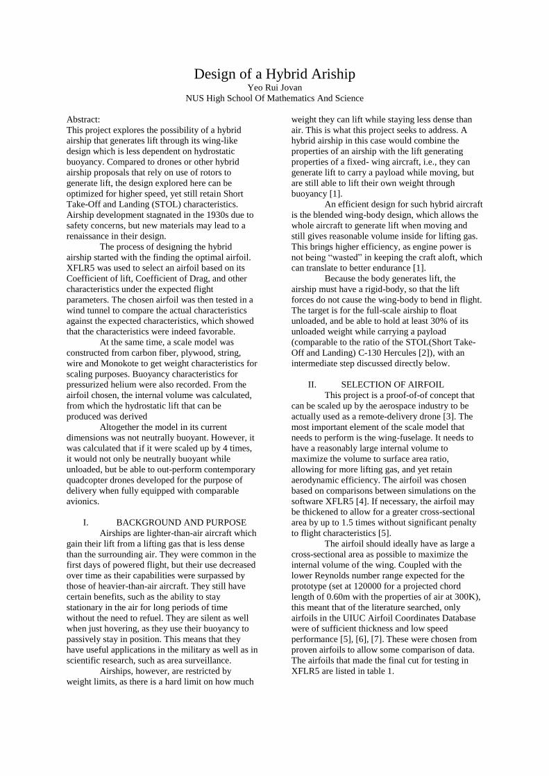
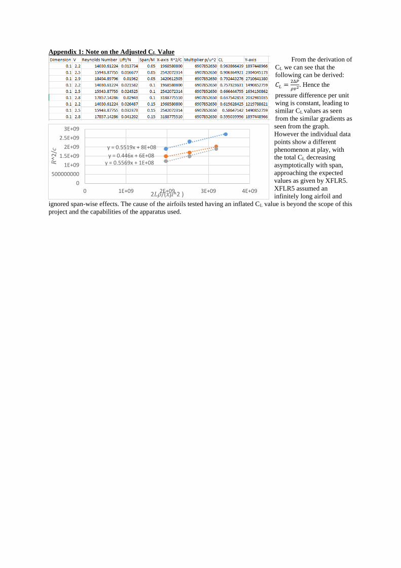
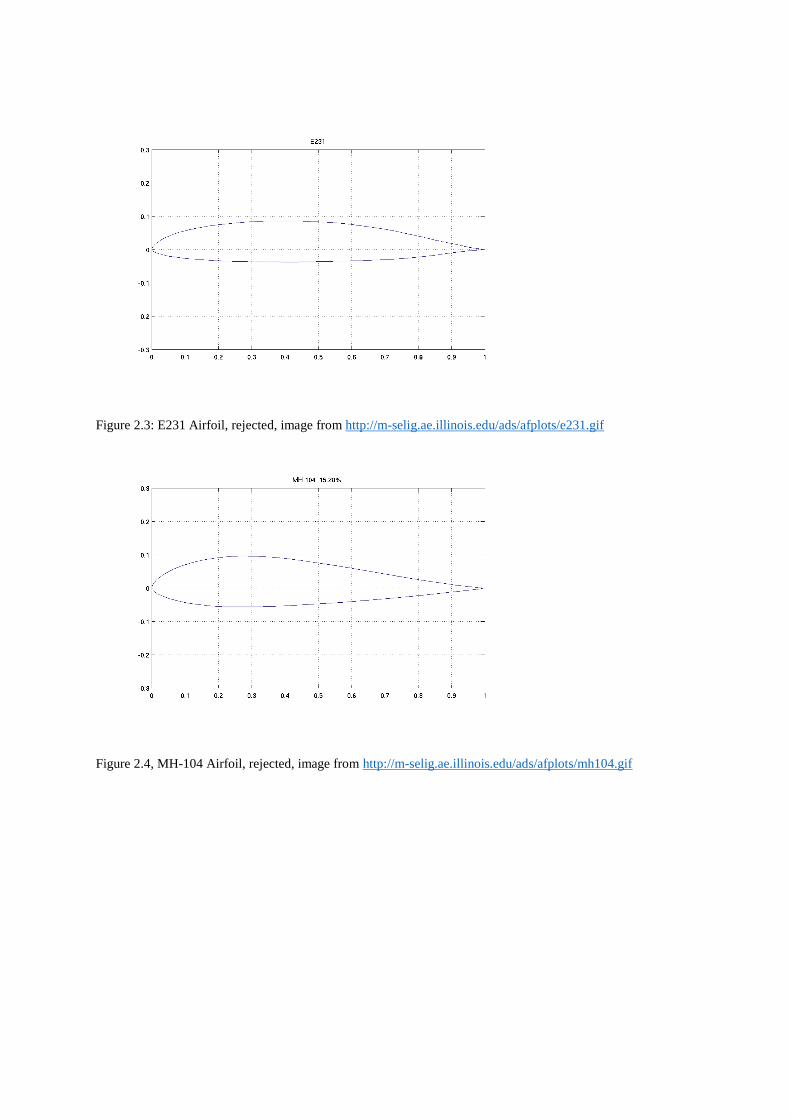
747A315 Eppler 23

MH-104

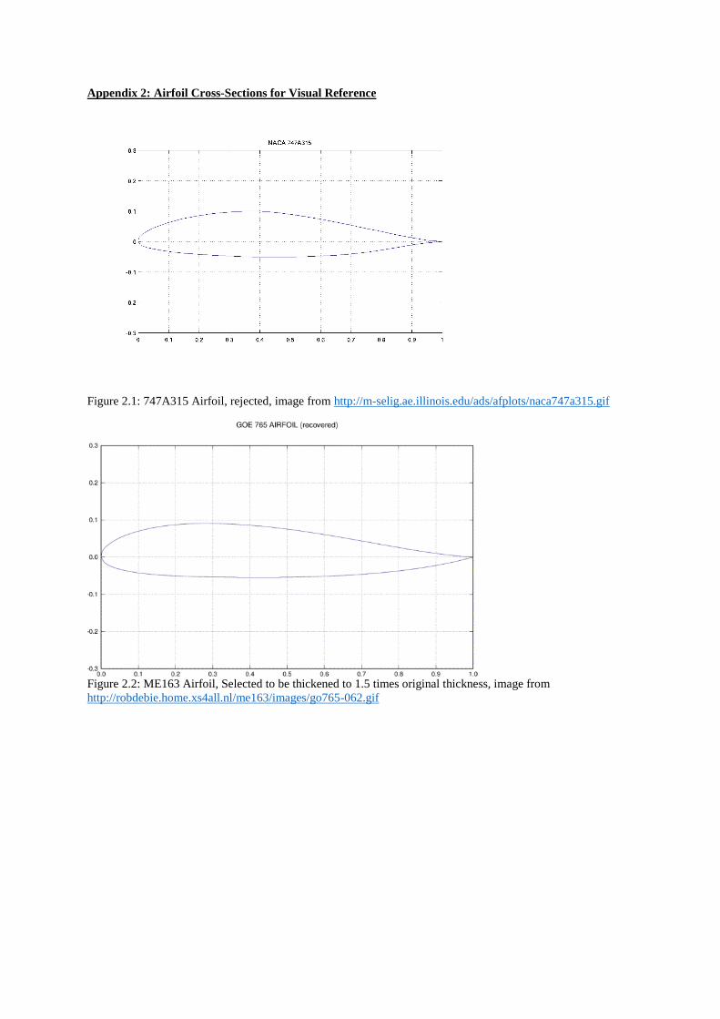
Göttingen 765

airfoil,

abbreviated to

ME163 based

on its

historical use

in this paper

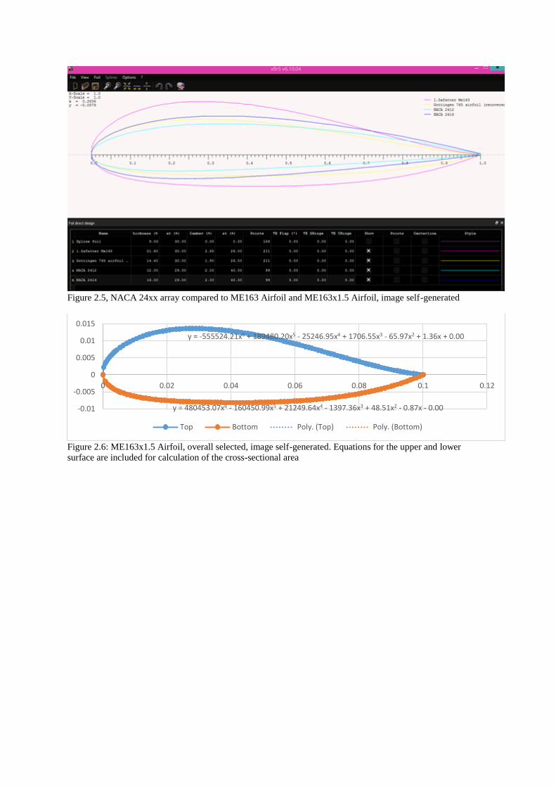
Table 1: Profiles of Airfoils used

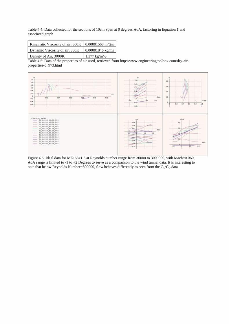
III. SIMULATION OF

PERFORMANCE PARAMETERS

XFLR5 is a software that allows for the

calculation of Coefficients of Lift, Drag, Moment,

and airflow properties based on user-defined data

such as Mach, Reynold’s number, and Angle of

attack, amongst others. For the purposes of this

project, the parameters that were compared were:

(i) the CL against AoA, (ii) CL against CD and (iii)

CL/CD against AoA.

The comparison of selected airfoils was

done in an elimination fashion to reduce demands

on the software. Below is the reason why one

airfoil was chosen over the other, based on the

simulation provided by XFLR5, as well as the

reason why it was chosen. Reynolds number range

was 20000 to 200000, with Mach=0.060 to reflect

the likely full-scale parameters. The corresponding

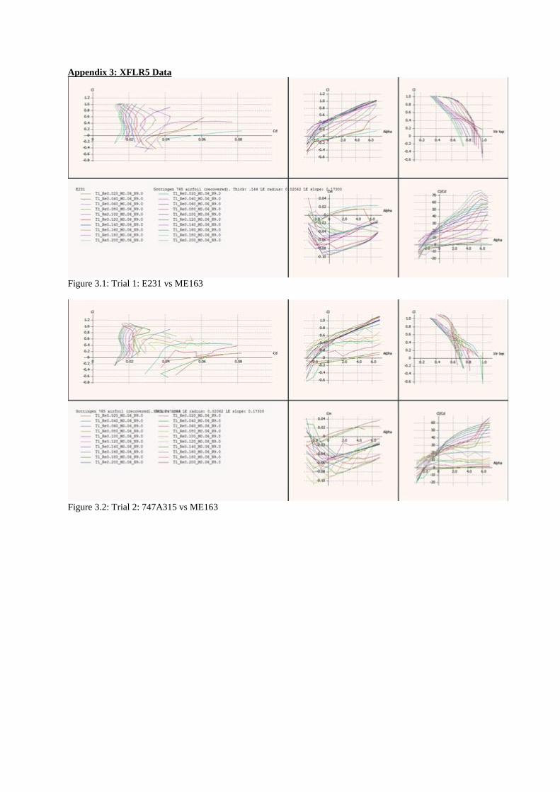
XFLR5 data is in Appendix 2.

Trial 1: E231 vs ME163. Both show similar

performance in all parameters, but ME163 has the

greater cross sectional area of the two, hence E231

was eliminated

Trial 2: 747A315 vs ME163. ME163 shows

generally better performance in all three

parameters, hence 747A315 was eliminated.

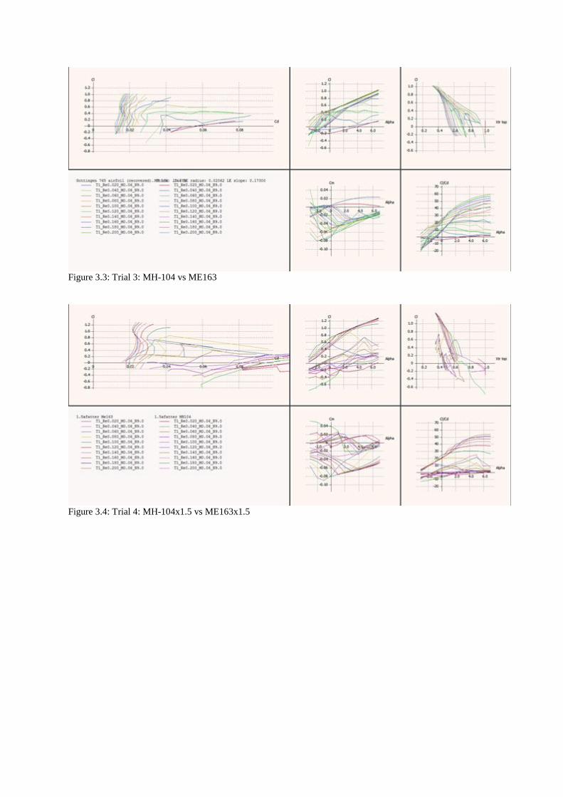
Trial 3: MH-104 vs ME163: Both show similar

performance in all parameters, so both were

selected for thickening and retesting. Thickening

notation for this report is <Name of

airfoil>x<Ratio>.

Trial 4: MH-104x1.5 vs ME163x1.5: ME163

retains superior performance in all parameters more

effectively when scaling, hence it is chosen over

MH-104.

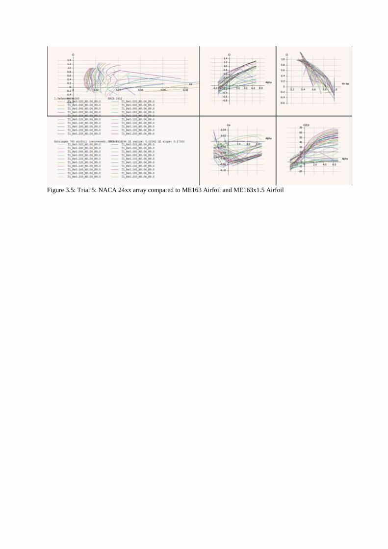
Trial 5: NACA 24xx array compared to ME163

and ME163x1.5: As in Trial 1, both have similar

performance in all parameters, but ME163x 1.5 has

a greater cross-sectional area. Hence, Me163x 1.5

was the canidate chosen for wind tunnel trials.

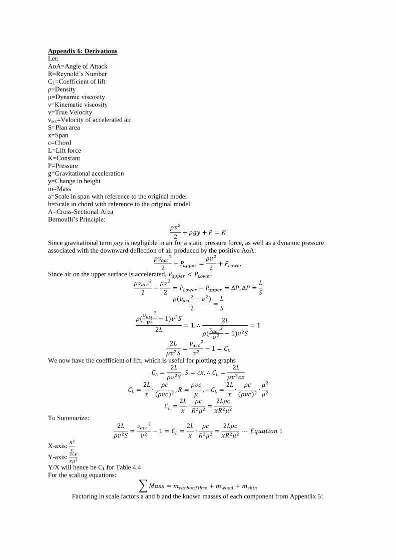
IV. THEORETICAL BASIS OF

CALCULATIONS

We assume that lift can be calculated with

Bernoulli’s Principle, where 𝜌𝑣2

2+ 𝜌𝑔𝑦 + 𝑃 is a

constant K, and the gravitational term ρgy is

negligible in air for a static pressure force, as well

as the dynamic pressure associated with the

downward deflection of air produced by the

positive AoA. The following can hence be derived: 𝜌(𝑣𝑎𝑐𝑐

2−𝑣2)

2=

𝐿

𝑆, and from which we can obtain an

expression for coefficient of lift at 0 degrees AoA: 2𝐿

𝜌𝑣2𝑆=

𝑣𝑎𝑐𝑐2

𝑣2− 1 = 𝐶𝐿 =

2𝐿

𝑥∙

𝜌𝑐

𝑅2𝜇2=

2𝐿𝜌𝑐

𝑥𝑅2𝜇2

We therefore expect the lift to increase with the

square of the Reynold’s Number (A full derivation

is available in Appendix 6).

V. EXPERIMENTAL TESTING OF

MODEL

Once the airfoil was chosen, the surface

area and volume of the model was calculated. To

simplify construction, no wing tapering or sweep

was used. Wind tunnel tests of the selected design

were performed to confirm the data, using two

kinds of models: one to test mass predictions and

one to test aerodynamic performance.

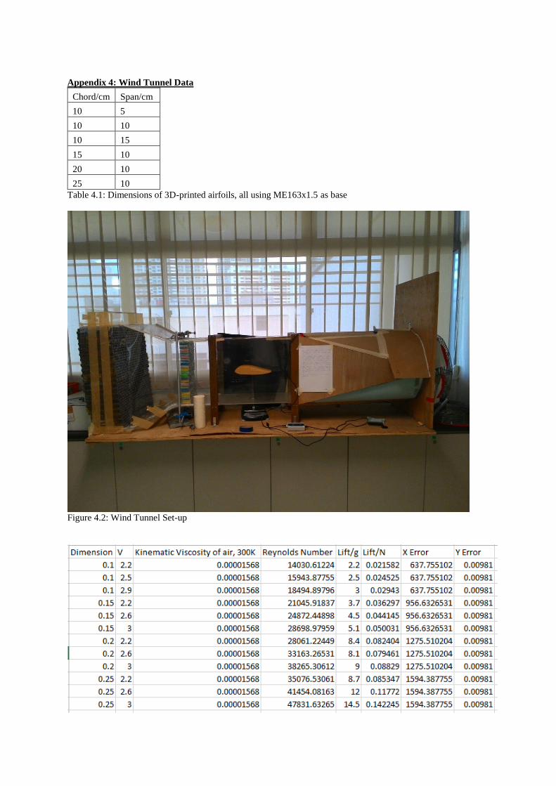
The wind tunnel is a refurbished wind

tunnel left behind from an unrelated student’s

project. It was modified to include a weighing scale

with an accuracy of 0.1g and an anemometer with

an accuracy of 0.1m/s. It has 3 speed settings,

which are 2.2m/s, 2.5-2.6m/s, and 2.9-3m/s

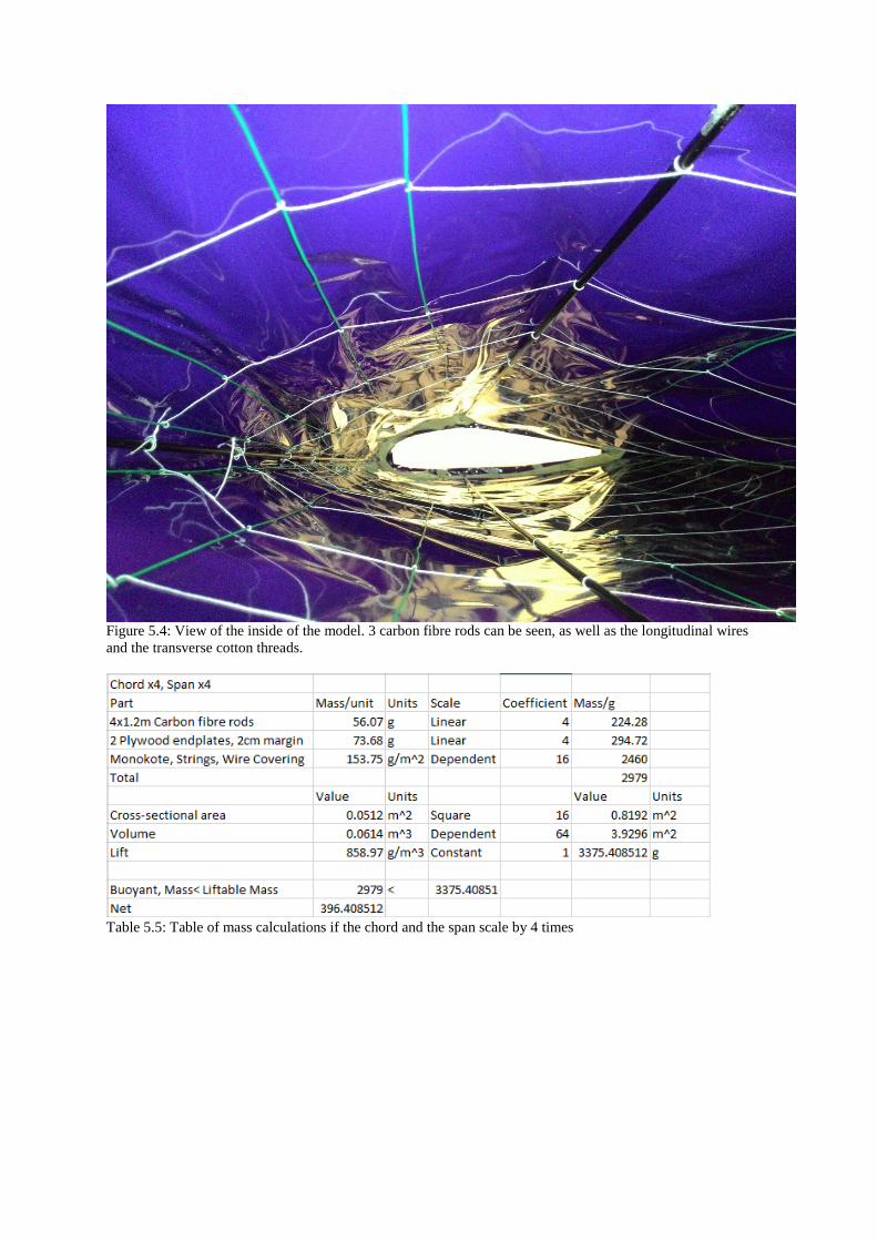
For mass predictions, the model’s weight was

recorded throughout the construction process.

Calibration of the lifting potential of helium also

occurred. It consists of two wooden chord panels

on either end to provide the shape of the airfoil

which are held together by 4 carbon fiber rods to

provide rigidity. To maintain the shape of the

airfoil, metal wire is laid at strategic points

longitudinally and cotton thread is laid

transversally. The inside was hollow so that gas

sacs. Each plywood panel has its center cut out to

leave a 2cm thick inner margin.

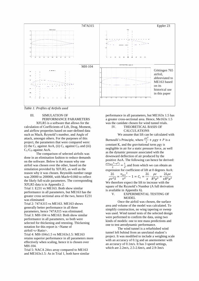
VI. AERODYNAMIC TESTING AND

RESULTS

Figure 1 Graph of Lift against Reynold's Number

3D-printed airfoil sections of ME163x1.5

were made for wind tunnel usage. Their

dimensions are listed in Appendix 4.

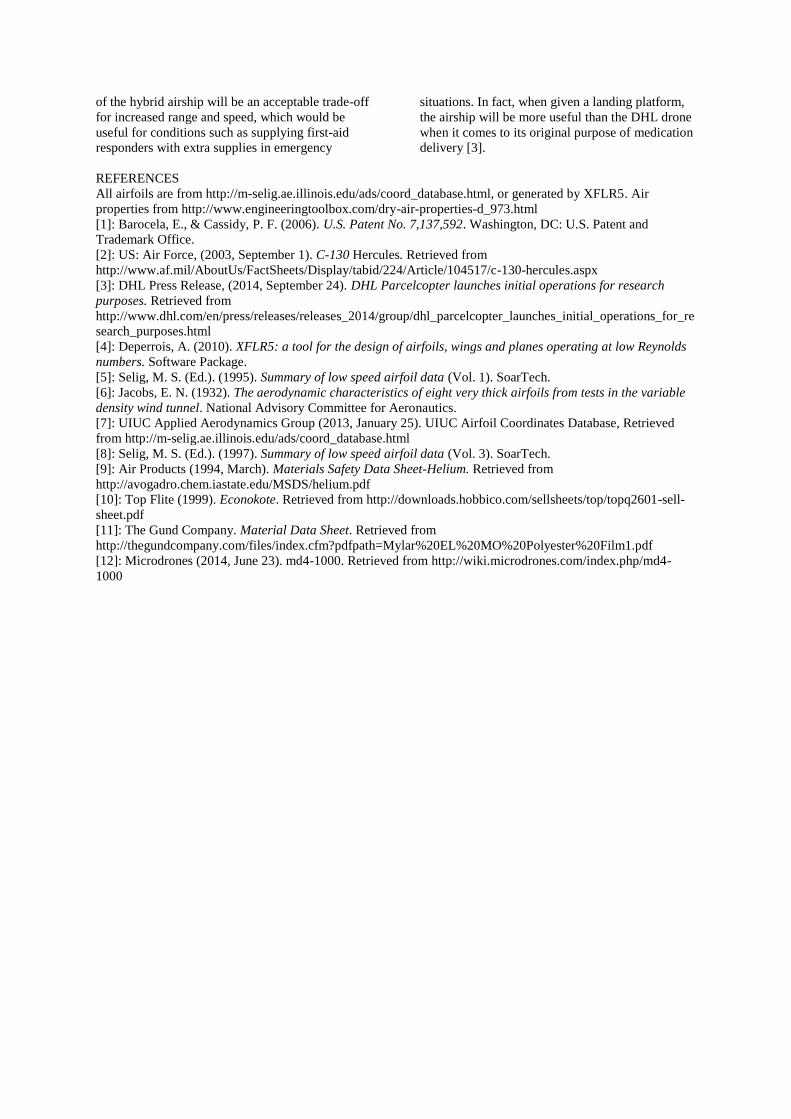
The following table plotted from Table 4.3 in

Appendix 4 shows the power relation between

Reynold’s Number and Lift force. This graph

shows a close fit to the predicted trendline of

Equation 1.

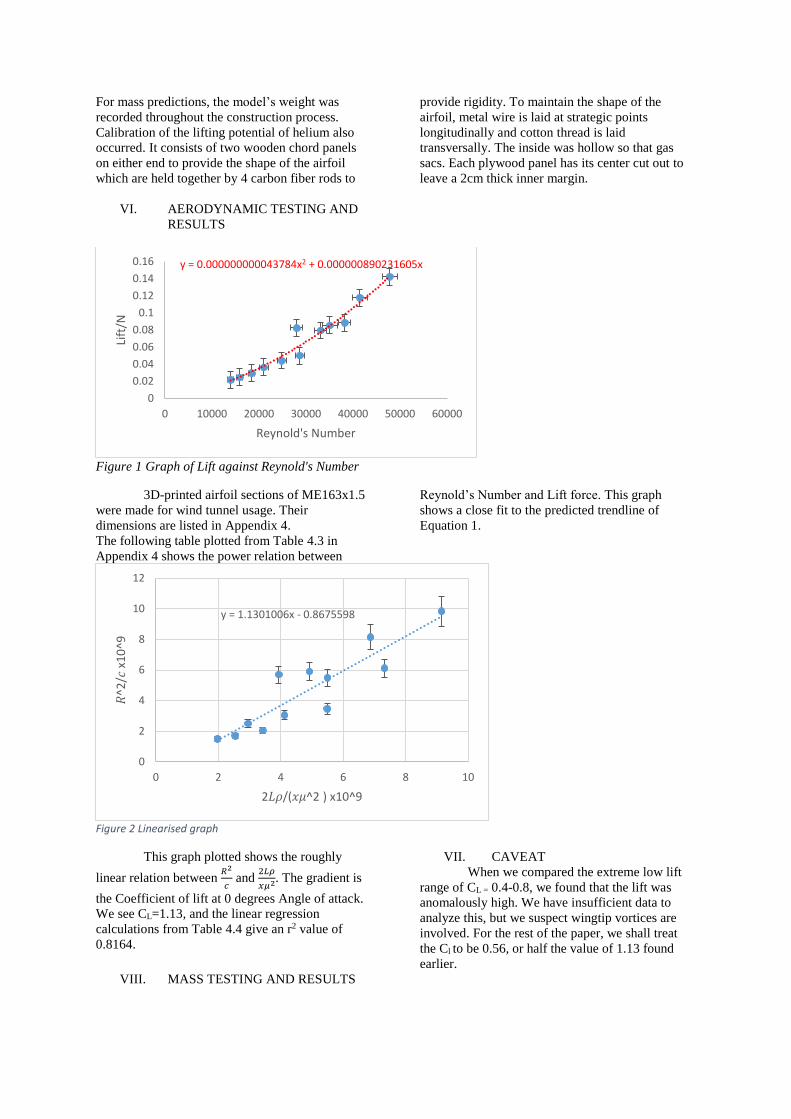
Figure 2 Linearised graph

This graph plotted shows the roughly

linear relation between 𝑅2

𝑐 and

2𝐿𝜌

𝑥𝜇2. The gradient is

the Coefficient of lift at 0 degrees Angle of attack.

We see CL=1.13, and the linear regression

calculations from Table 4.4 give an r2 value of

0.8164.

VII. CAVEAT

When we compared the extreme low lift

range of CL = 0.4-0.8, we found that the lift was

anomalously high. We have insufficient data to

analyze this, but we suspect wingtip vortices are

involved. For the rest of the paper, we shall treat

the Cl to be 0.56, or half the value of 1.13 found

earlier.

VIII. MASS TESTING AND RESULTS

y = 0.000000000043784x2 + 0.000000890231605x

0

0.02

0.04

0.06

0.08

0.1

0.12

0.14

0.16

0 10000 20000 30000 40000 50000 60000

Lift

/N

Reynold's Number

y = 1.1301006x - 0.8675598

0

2

4

6

8

10

12

0 2 4 6 8 10

𝑅^2

/𝑐x1

0^9

2𝐿𝜌/(𝑥𝜇^2 ) x10^9

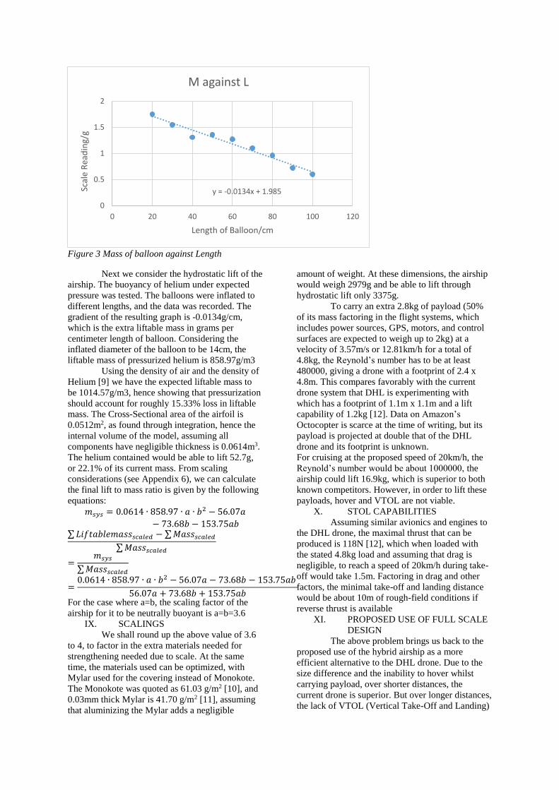
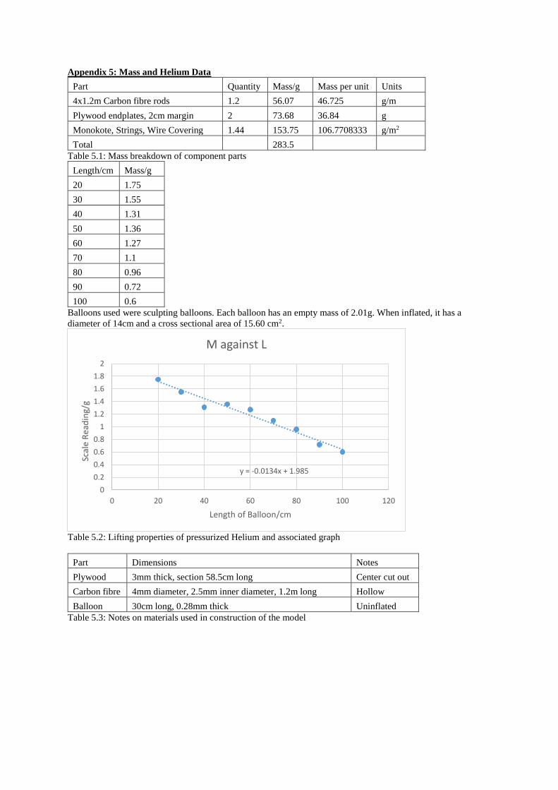
Figure 3 Mass of balloon against Length

Next we consider the hydrostatic lift of the

airship. The buoyancy of helium under expected

pressure was tested. The balloons were inflated to

different lengths, and the data was recorded. The

gradient of the resulting graph is -0.0134g/cm,

which is the extra liftable mass in grams per

centimeter length of balloon. Considering the

inflated diameter of the balloon to be 14cm, the

liftable mass of pressurized helium is 858.97g/m3

Using the density of air and the density of

Helium [9] we have the expected liftable mass to

be 1014.57g/m3, hence showing that pressurization

should account for roughly 15.33% loss in liftable

mass. The Cross-Sectional area of the airfoil is

0.0512m2, as found through integration, hence the

internal volume of the model, assuming all

components have negligible thickness is 0.0614m3.

The helium contained would be able to lift 52.7g,

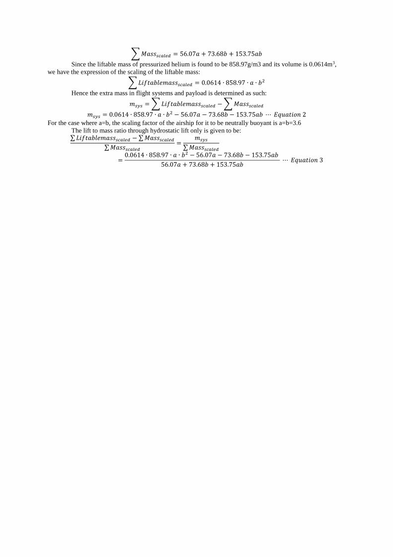
or 22.1% of its current mass. From scaling

considerations (see Appendix 6), we can calculate

the final lift to mass ratio is given by the following

equations:

𝑚𝑠𝑦𝑠 = 0.0614 ∙ 858.97 ∙ 𝑎 ∙ 𝑏2 − 56.07𝑎

− 73.68𝑏 − 153.75𝑎𝑏

∑ 𝐿𝑖𝑓𝑡𝑎𝑏𝑙𝑒𝑚𝑎𝑠𝑠𝑠𝑐𝑎𝑙𝑒𝑑 − ∑ 𝑀𝑎𝑠𝑠𝑠𝑐𝑎𝑙𝑒𝑑

∑ 𝑀𝑎𝑠𝑠𝑠𝑐𝑎𝑙𝑒𝑑

=𝑚𝑠𝑦𝑠

∑ 𝑀𝑎𝑠𝑠𝑠𝑐𝑎𝑙𝑒𝑑

=0.0614 ∙ 858.97 ∙ 𝑎 ∙ 𝑏2 − 56.07𝑎 − 73.68𝑏 − 153.75𝑎𝑏

56.07𝑎 + 73.68𝑏 + 153.75𝑎𝑏

For the case where a=b, the scaling factor of the

airship for it to be neutrally buoyant is a=b=3.6

IX. SCALINGS

We shall round up the above value of 3.6

to 4, to factor in the extra materials needed for

strengthening needed due to scale. At the same

time, the materials used can be optimized, with

Mylar used for the covering instead of Monokote.

The Monokote was quoted as 61.03 g/m2 [10], and

0.03mm thick Mylar is 41.70 g/m2 [11], assuming

that aluminizing the Mylar adds a negligible

amount of weight. At these dimensions, the airship

would weigh 2979g and be able to lift through

hydrostatic lift only 3375g.

To carry an extra 2.8kg of payload (50%

of its mass factoring in the flight systems, which

includes power sources, GPS, motors, and control

surfaces are expected to weigh up to 2kg) at a

velocity of 3.57m/s or 12.81km/h for a total of

4.8kg, the Reynold’s number has to be at least

480000, giving a drone with a footprint of 2.4 x

4.8m. This compares favorably with the current

drone system that DHL is experimenting with

which has a footprint of 1.1m x 1.1m and a lift

capability of 1.2kg [12]. Data on Amazon’s

Octocopter is scarce at the time of writing, but its

payload is projected at double that of the DHL

drone and its footprint is unknown.

For cruising at the proposed speed of 20km/h, the

Reynold’s number would be about 1000000, the

airship could lift 16.9kg, which is superior to both

known competitors. However, in order to lift these

payloads, hover and VTOL are not viable.

X. STOL CAPABILITIES

Assuming similar avionics and engines to

the DHL drone, the maximal thrust that can be

produced is 118N [12], which when loaded with

the stated 4.8kg load and assuming that drag is

negligible, to reach a speed of 20km/h during take-

off would take 1.5m. Factoring in drag and other

factors, the minimal take-off and landing distance

would be about 10m of rough-field conditions if

reverse thrust is available

XI. PROPOSED USE OF FULL SCALE

DESIGN

The above problem brings us back to the

proposed use of the hybrid airship as a more

efficient alternative to the DHL drone. Due to the

size difference and the inability to hover whilst

carrying payload, over shorter distances, the

current drone is superior. But over longer distances,

the lack of VTOL (Vertical Take-Off and Landing)

y = -0.0134x + 1.985

0

0.5

1

1.5

2

0 20 40 60 80 100 120

Scal

e R

ead

ing/

g

Length of Balloon/cm

M against L

of the hybrid airship will be an acceptable trade-off

for increased range and speed, which would be

useful for conditions such as supplying first-aid

responders with extra supplies in emergency

situations. In fact, when given a landing platform,

the airship will be more useful than the DHL drone

when it comes to its original purpose of medication

delivery [3].

REFERENCES

All airfoils are from http://m-selig.ae.illinois.edu/ads/coord_database.html, or generated by XFLR5. Air

properties from http://www.engineeringtoolbox.com/dry-air-properties-d_973.html

[1]: Barocela, E., & Cassidy, P. F. (2006). U.S. Patent No. 7,137,592. Washington, DC: U.S. Patent and

Trademark Office.

[2]: US: Air Force, (2003, September 1). C-130 Hercules. Retrieved from

http://www.af.mil/AboutUs/FactSheets/Display/tabid/224/Article/104517/c-130-hercules.aspx

[3]: DHL Press Release, (2014, September 24). DHL Parcelcopter launches initial operations for research

purposes. Retrieved from

http://www.dhl.com/en/press/releases/releases_2014/group/dhl_parcelcopter_launches_initial_operations_for_re

search_purposes.html

[4]: Deperrois, A. (2010). XFLR5: a tool for the design of airfoils, wings and planes operating at low Reynolds

numbers. Software Package.

[5]: Selig, M. S. (Ed.). (1995). Summary of low speed airfoil data (Vol. 1). SoarTech.

[6]: Jacobs, E. N. (1932). The aerodynamic characteristics of eight very thick airfoils from tests in the variable

density wind tunnel. National Advisory Committee for Aeronautics.

[7]: UIUC Applied Aerodynamics Group (2013, January 25). UIUC Airfoil Coordinates Database, Retrieved

from http://m-selig.ae.illinois.edu/ads/coord_database.html

[8]: Selig, M. S. (Ed.). (1997). Summary of low speed airfoil data (Vol. 3). SoarTech.

[9]: Air Products (1994, March). Materials Safety Data Sheet-Helium. Retrieved from

http://avogadro.chem.iastate.edu/MSDS/helium.pdf

[10]: Top Flite (1999). Econokote. Retrieved from http://downloads.hobbico.com/sellsheets/top/topq2601-sell-

sheet.pdf

[11]: The Gund Company. Material Data Sheet. Retrieved from

http://thegundcompany.com/files/index.cfm?pdfpath=Mylar%20EL%20MO%20Polyester%20Film1.pdf

[12]: Microdrones (2014, June 23). md4-1000. Retrieved from http://wiki.microdrones.com/index.php/md4-

1000

Appendix 1: Note on the Adjusted CL Value

From the derivation of

CL we can see that the

following can be derived:

𝐶𝐿 =2∆𝑃

𝜌𝑣2. Hence the

pressure difference per unit

wing is constant, leading to

similar CL values as seen

from the similar gradients as

seen from the graph.

However the individual data

points show a different

phenomenon at play, with

the total CL decreasing

asymptotically with span,

approaching the expected

values as given by XFLR5.

XFLR5 assumed an

infinitely long airfoil and

ignored span-wise effects. The cause of the airfoils tested having an inflated CL value is beyond the scope of this

project and the capabilities of the apparatus used.

y = 0.5519x + 8E+08

y = 0.446x + 6E+08y = 0.5569x + 1E+08

0

500000000

1E+09

1.5E+09

2E+09

2.5E+09

3E+09

0 1E+09 2E+09 3E+09 4E+09

𝑅^2

/𝑐

2𝐿𝜌/(𝑥𝜇^2 )

Appendix 2: Airfoil Cross-Sections for Visual Reference

Figure 2.1: 747A315 Airfoil, rejected, image from http://m-selig.ae.illinois.edu/ads/afplots/naca747a315.gif

Figure 2.2: ME163 Airfoil, Selected to be thickened to 1.5 times original thickness, image from

http://robdebie.home.xs4all.nl/me163/images/go765-062.gif

Figure 2.3: E231 Airfoil, rejected, image from http://m-selig.ae.illinois.edu/ads/afplots/e231.gif

Figure 2.4, MH-104 Airfoil, rejected, image from http://m-selig.ae.illinois.edu/ads/afplots/mh104.gif

Figure 2.5, NACA 24xx array compared to ME163 Airfoil and ME163x1.5 Airfoil, image self-generated

Figure 2.6: ME163x1.5 Airfoil, overall selected, image self-generated. Equations for the upper and lower

surface are included for calculation of the cross-sectional area

y = -555524.21x6 + 189480.20x5 - 25246.95x4 + 1706.55x3 - 65.97x2 + 1.36x + 0.00

y = 480453.07x6 - 160450.99x5 + 21249.64x4 - 1397.36x3 + 48.51x2 - 0.87x - 0.00-0.01

-0.005

0

0.005

0.01

0.015

0 0.02 0.04 0.06 0.08 0.1 0.12

Top Bottom Poly. (Top) Poly. (Bottom)

Appendix 3: XFLR5 Data

Figure 3.1: Trial 1: E231 vs ME163

Figure 3.2: Trial 2: 747A315 vs ME163

Figure 3.3: Trial 3: MH-104 vs ME163

Figure 3.4: Trial 4: MH-104x1.5 vs ME163x1.5

Figure 3.5: Trial 5: NACA 24xx array compared to ME163 Airfoil and ME163x1.5 Airfoil

Appendix 4: Wind Tunnel Data

Chord/cm Span/cm

10 5

10 10

10 15

15 10

20 10

25 10

Table 4.1: Dimensions of 3D-printed airfoils, all using ME163x1.5 as base

Figure 4.2: Wind Tunnel Set-up

Table 4.3: Data collected for the sections of 10cm Span at 0 degrees Angle of attack and associated graph

y = 0.000000000043784x2 + 0.000000890231605x

0

0.02

0.04

0.06

0.08

0.1

0.12

0.14

0.16

0 10000 20000 30000 40000 50000 60000

Lift

/N

Reynold's Number

y = 1.1301006x - 0.8675598

0

2

4

6

8

10

12

0 1 2 3 4 5 6 7 8 9 10

𝑅^2

/𝑐x1

0^9

2𝐿𝜌/(𝑥𝜇^2 ) x10^9

Table 4.4: Data collected for the sections of 10cm Span at 0 degrees AoA, factoring in Equation 1 and

associated graph

Kinematic Viscosity of air, 300K 0.00001568 m^2/s

Dynamic Viscosity of air, 300K 0.00001846 kg/ms

Density of Air, 3000K 1.177 kg/m^3

Table 4.5: Data of the properties of air used, retrieved from http://www.engineeringtoolbox.com/dry-air-

properties-d_973.html

Figure 4.6: Ideal data for ME163x1.5 at Reynolds number range from 30000 to 3000000, with Mach=0.060,

AoA range is limited to -1 to +2 Degrees to serve as a comparison to the wind tunnel data. It is interesting to

note that below Reynolds Number=800000, flow behaves differently as seen from the CL/CD data

Appendix 5: Mass and Helium Data

Part Quantity Mass/g Mass per unit Units

4x1.2m Carbon fibre rods 1.2 56.07 46.725 g/m

Plywood endplates, 2cm margin 2 73.68 36.84 g

Monokote, Strings, Wire Covering 1.44 153.75 106.7708333 g/m2

Total 283.5

Table 5.1: Mass breakdown of component parts

Length/cm Mass/g

20 1.75

30 1.55

40 1.31

50 1.36

60 1.27

70 1.1

80 0.96

90 0.72

100 0.6

Balloons used were sculpting balloons. Each balloon has an empty mass of 2.01g. When inflated, it has a

diameter of 14cm and a cross sectional area of 15.60 cm2.

Table 5.2: Lifting properties of pressurized Helium and associated graph

Part Dimensions Notes

Plywood 3mm thick, section 58.5cm long Center cut out

Carbon fibre 4mm diameter, 2.5mm inner diameter, 1.2m long Hollow

Balloon 30cm long, 0.28mm thick Uninflated

Table 5.3: Notes on materials used in construction of the model

y = -0.0134x + 1.985

0

0.2

0.4

0.6

0.8

1

1.2

1.4

1.6

1.8

2

0 20 40 60 80 100 120

Scal

e R

ead

ing/

g

Length of Balloon/cm

M against L

Figure 5.4: View of the inside of the model. 3 carbon fibre rods can be seen, as well as the longitudinal wires

and the transverse cotton threads.

Table 5.5: Table of mass calculations if the chord and the span scale by 4 times

Appendix 6: Derivations Let:

AoA=Angle of Attack

R=Reynold’s Number

CL=Coefficient of lift

ρ=Density

μ=Dynamic viscosity

ν=Kinematic viscosity

v=True Velocity

vacc=Velocity of accelerated air

S=Plan area

x=Span

c=Chord

L=Lift force

K=Constant

P=Pressure

g=Gravitational acceleration

y=Change in height

m=Mass

a=Scale in span with reference to the original model

b=Scale in chord with reference to the original model

A=Cross-Sectional Area

Bernoulli’s Principle:

𝜌𝑣2

2+ 𝜌𝑔𝑦 + 𝑃 = 𝐾

Since gravitational term ρgy is negligible in air for a static pressure force, as well as a dynamic pressure

associated with the downward deflection of air produced by the positive AoA:

𝜌𝑣𝑎𝑐𝑐2

2+ 𝑃𝑢𝑝𝑝𝑒𝑟 =

𝜌𝑣2

2+ 𝑃𝐿𝑜𝑤𝑒𝑟

Since air on the upper surface is accelerated, 𝑃𝑢𝑝𝑝𝑒𝑟 < 𝑃𝐿𝑜𝑤𝑒𝑟

𝜌𝑣𝑎𝑐𝑐2

2−

𝜌𝑣2

2= 𝑃𝐿𝑜𝑤𝑒𝑟 − 𝑃𝑢𝑝𝑝𝑒𝑟 = ∆𝑃, ∆𝑃 =

𝐿

𝑆

𝜌(𝑣𝑎𝑐𝑐2 − 𝑣2)

2=

𝐿

𝑆

𝜌(𝑣𝑎𝑐𝑐

2

𝑣2 − 1)𝑣2𝑆

2𝐿= 1, ∴

2𝐿

𝜌(𝑣𝑎𝑐𝑐

2

𝑣2 − 1)𝑣2𝑆= 1

2𝐿

𝜌𝑣2𝑆=

𝑣𝑎𝑐𝑐2

𝑣2− 1 = 𝐶𝐿

We now have the coefficient of lift, which is useful for plotting graphs

𝐶𝐿 =2𝐿

𝜌𝑣2𝑆, 𝑆 = 𝑐𝑥, ∴ 𝐶𝐿 =

2𝐿

𝜌𝑣2𝑐𝑥

𝐶𝐿 =2𝐿

𝑥∙

𝜌𝑐

(𝜌𝑣𝑐)2, 𝑅 =

𝜌𝑣𝑐

𝜇, ∴ 𝐶𝐿 =

2𝐿

𝑥∙

𝜌𝑐

(𝜌𝑣𝑐)2∙

𝜇2

𝜇2

𝐶𝐿 =2𝐿

𝑥∙

𝜌𝑐

𝑅2𝜇2=

2𝐿𝜌𝑐

𝑥𝑅2𝜇2

To Summarize:

2𝐿

𝜌𝑣2𝑆=

𝑣𝑎𝑐𝑐2

𝑣2− 1 = 𝐶𝐿 =

2𝐿

𝑥∙

𝜌𝑐

𝑅2𝜇2=

2𝐿𝜌𝑐

𝑥𝑅2𝜇2 ⋯ 𝐸𝑞𝑢𝑎𝑡𝑖𝑜𝑛 1

X-axis: 𝑅2

𝑐

Y-axis: 2𝐿𝜌

𝑥𝜇2

Y/X will hence be CL for Table 4.4

For the scaling equations:

∑ 𝑀𝑎𝑠𝑠 = 𝑚𝑐𝑎𝑟𝑏𝑜𝑛𝑓𝑖𝑏𝑟𝑒 + 𝑚𝑤𝑜𝑜𝑑 + 𝑚𝑠𝑘𝑖𝑛

Factoring in scale factors a and b and the known masses of each component from Appendix 5:

∑ 𝑀𝑎𝑠𝑠𝑠𝑐𝑎𝑙𝑒𝑑 = 56.07𝑎 + 73.68𝑏 + 153.75𝑎𝑏

Since the liftable mass of pressurized helium is found to be 858.97g/m3 and its volume is 0.0614m3,

we have the expression of the scaling of the liftable mass:

∑ 𝐿𝑖𝑓𝑡𝑎𝑏𝑙𝑒𝑚𝑎𝑠𝑠𝑠𝑐𝑎𝑙𝑒𝑑 = 0.0614 ∙ 858.97 ∙ 𝑎 ∙ 𝑏2

Hence the extra mass in flight systems and payload is determined as such:

𝑚𝑠𝑦𝑠 = ∑ 𝐿𝑖𝑓𝑡𝑎𝑏𝑙𝑒𝑚𝑎𝑠𝑠𝑠𝑐𝑎𝑙𝑒𝑑 − ∑ 𝑀𝑎𝑠𝑠𝑠𝑐𝑎𝑙𝑒𝑑

𝑚𝑠𝑦𝑠 = 0.0614 ∙ 858.97 ∙ 𝑎 ∙ 𝑏2 − 56.07𝑎 − 73.68𝑏 − 153.75𝑎𝑏 ⋯ 𝐸𝑞𝑢𝑎𝑡𝑖𝑜𝑛 2

For the case where a=b, the scaling factor of the airship for it to be neutrally buoyant is a=b=3.6

The lift to mass ratio through hydrostatic lift only is given to be: ∑ 𝐿𝑖𝑓𝑡𝑎𝑏𝑙𝑒𝑚𝑎𝑠𝑠𝑠𝑐𝑎𝑙𝑒𝑑 − ∑ 𝑀𝑎𝑠𝑠𝑠𝑐𝑎𝑙𝑒𝑑

∑ 𝑀𝑎𝑠𝑠𝑠𝑐𝑎𝑙𝑒𝑑

=𝑚𝑠𝑦𝑠

∑ 𝑀𝑎𝑠𝑠𝑠𝑐𝑎𝑙𝑒𝑑

=0.0614 ∙ 858.97 ∙ 𝑎 ∙ 𝑏2 − 56.07𝑎 − 73.68𝑏 − 153.75𝑎𝑏

56.07𝑎 + 73.68𝑏 + 153.75𝑎𝑏 ⋯ 𝐸𝑞𝑢𝑎𝑡𝑖𝑜𝑛 3