DESIGN OF A SIMULATOR OF A RESERVOIR · PDF fileInternational Journal of Engineering and...

International Journal of Engineering and Advanced Technology Studies

Vol.4, No.4, pp.36-64, September 2016

___Published by European Centre for Research Training and Development UK (www.eajournals.org)

36 ISSN 2053¬5783(Print), ISSN 2053¬5791(online)

DESIGN OF A SIMULATOR OF A RESERVOIR INVESTIGATING THE EFFECT OF

SURFACTANT MIXTURE IN AN ENHANCED OIL RECOVERY PROCESS

Kamilu Folorunsho Oyedeko1 and Alfred Akpoveta Susu

2

1Department of Chemical & Polymer Engineering, Lagos State University, Epe, Lagos, Nigeria

2Department of Chemical Engineering, University of Lagos, Lagos, Nigeria

E-mail:[email protected]; [email protected]

ABSTRACT: In this paper, we present development of a simulator for multidimensional,

multiphase and multicomponent surfactant flooding concerned with the characteristics of the

chemical slugs for an enhanced oil recovery process. The development starts with the description

of the fluid flow in permeable media from the basic conservation laws and with linear

constitutive theory. From this physical basis a mathematical formulation of the flow problem

may be posed in the form of an initial-boundary value system of partial differential equations.

The form is presented in detail for the general multicomponent, multiphase system and several

special cases. A surfactant flood model for a two or three dimensions, two fluid phases (aqueous,

oleic) and one adsorbent phase and four components (oil, water, surfactants 1 and 2) system is

presented and analyzed. It is ruled by a system of non-linear, partial, differential equations; the

continuity equation for the transport of each component, Darcy’s equation for the flow of each

phase and algebraic equations. This system is numerically solved in the one-dimensional case.

The orthogonal collocation and finite difference techniques were used in solving the equations

that characterized the multidimensional, multiphase and multicomponent flow problem. The

simulator is fed with the physical properties that are concentration dependent functions. The

material transport equations are decoupled from the momentum transport equations and the

complex, time changing flow-field requires a numerical solution. Matlab computer programs

were used for the numerical solution of the model equations. The results of the orthogonal

collocation solution were compared with those of finite difference solutions. The results indicate

that the concentration of surfactants for orthogonal collocation show more features than the

predictions of the finite difference, offering more opportunities for further understanding of the

physical nature of the complex problem and chemical effectiveness. Also, comparison of the

orthogonal collocation solution with computations based on finite difference method offers

possible explanation for the observed differences especially between the methods and the two

reservoirs.

KEYWORDS: Chemical flooding, Surfactant, Multicomponent, Multidimensional and

Multiphase System, Orthogonal Collocation Technique, Finite Difference Method





INTRODUCTION

The study of displacement process required the understanding of the porous formation of

complex reservoir and multiphase and multicomponent flow taking place in the reservoir. This is

essential for development of a simulator of a reservoir in a surfactant assisted waterflood.

In order to maximize oil recovery from reservoirs, operators consider Enhanced Oil Recovery as

effective method. Also increasing high oil prices and declining production in many regions

around the globe makes this advance technologies called “Enhanced Oil Recovery“(EOR) of

recovering trapped oil in reservoir attractive for exploration and production operations.This

implies the injection of a fluid or fluids or materials into a reservoir to supplement the natural

energy present in a reservoir, where the injected fluids interact with the reservoir rock /oil /brine

system to create favourable conditions for maximum oil recovery [1,2]

The technical insights into enhanced oil recovery technologies are developed to increase the

extraction of crude oil from reservoirs after primary production. Since not all the original oil in

place can be recovered by the primary and secondary processes. Chemical enhanced oil recovery

is used to mobilize the trapped oil in reservoir pores after a secondary recovery after water

flooding. Surfactant flooding is a form of chemical flooding process. Surfactants are injected to

decrease the interfacial tension between oil and water in order to mobilize the oil trapped after

secondary recovery by water flooding.This is achieved by lowering the oil-water interfacial

tension and allowing oil to flow within the pores of reservoir rock and into the well bores.

In a surfactant flood, a multi-component multiphase system is involved. The theory of multi-

component, multiphase flow has been presented by several authors.The surfactant flooding is

represented by a system of nonlinear partial differential equations: the continuity equation for the

transport of the components and Darcy‟s equation for the phase flow [3]. The present work

describes the development of a simulator for an Enhanced Oil Recovery process for surfactant

assisted waterflooding by applying different mathematical methods, orthogonal collocation

method and finite difference methods to solve the basic model transport equations.The approach

adopted here involves the use of different mathematical techniques; orthogonal collocation

method and finite difference for the development and simulation of the relevant nonlinear partial

differential equations. The two mathematical techniques further less the burden in this complex

problem because of the multi-component, multiphase, multidimensional displacement

phenomena in porous systems.

The different mathematical techniques; orthogonal collocation method and finite difference are

to be utilized to identify a particular type of physical behaviour and enable the understanding of

the involved propagation phenomena in terms of cause and effects. More so, the techniques will

in particular be utilized to predict what happens in EOR process and show the complexity of the

problem can be reduced by intensive calculation.





This work applied different techniques; orthogonal collocation method and finite difference to

solve the basic model transport equations. The approach is multidimensional. It involved at least

three independent variables, which mean that the various composition path spaces required to

map the composition routes of the system are at most two dimensional, allowing for a great

simplification in complexity.

Systems of coupled, first-order, nonlinear hyperbolic partial differential equations (p.d.e.s)

govern the transient evolution of a chemical flooding process for enhanced recovery. The method

of characteristics (MOC) provides a way in which such systems of hyperbolic p.d.e.s can be

solved by converting them to an equivalent system of ordinary differential equations. In some

cases, the characteristic solution has been used to track the flood-front in two-dimensional

reservoir problems [4]. The characteristic method was combined with a finite element approach

to solve the problems [5]. The MOC and an adjustable number of moving particles were used to

track three-dimensional solute fronts in groundwater systems; adjusting the number of particles

serves to maintain an accurate material balance and save computational time [6].

At the simple level, the results of simulation using these techniques are analogous to the

Buckley-Leverett theory for waterflooding, the latter being evident in the work for polymer

flooding [7], for dilute surfactant flooding [8], for carbonated waterflooding [9], and for miscible

and immiscible surfactant flooding [10,11], for isothermal, multiphase, multicomponent fluid

flow in permeable media [12]. Also, Case studies for the feasibility of sweep improvement in

surfactant-assisted waterflooding [17].

High oil prices and declining production in many regions around the globe, makes enhanced oil

recovery (EOR) increasingly attractive for researchers. As evident in the work for a new class of

viscoelastic surfactants for EOR [14], for microbially enhanced oil recovery at simulated

reservoir conditions by use of engineered bacteria [15], for co-optimization of enhanced oil

recovery and carbon sequestration [16], for development of improved surfactants and EOR

methods for small operators [17]..

The present work describes the design of a simulator of reservoir using the effect of surfactant

mixture assisted water flooding an Enhanced Oil Recovery process by applying two different

mathematical methods, orthogonal collocation and finite difference method, to solve the basic

model transport equations. The approach is multidimensional and involves at least three

independent variables.

METHODOLOGY

This work considered the solution of a multidimensional, multicomponent and multiphase flow

problem associated with enhanced oil recovery process in petroleum engineering. The process of

interest involves the injection of surfactant of different concentrations and pore volume to

displace oil from the reservoir.

http://academic.research.microsoft.com/Publication/49451950/co-optimization-of-enhanced-oil-recovery-and-carbon-sequestration






The methodology used here is illustrated by the steps utilized in executing the solution using the

developed mathematical models describing the physics of reservoir depletion and fluid flow in

which one of the main aims is the determination of the areal distribution of fluids in the flooded

reservoir. The system is for two or three dimensions, two fluid phases (aqueous, oleic) and one

adsorbent phase, four components (oil, water, surfactants 1 and 2).

The reservoir may be divided into discrete grid blocks which may each be characterized by

having different reservoir properties. The flow of fluids from a block is governed by the principle

of mass conservation coupled with Darcy‟s law. The following are taken into consideration in

the modeling effort: (i) the simultaneous flow of oil, gas, and water in three dimensions, (ii) the

effects of natural water influx, fluid compressibility, mass transfer between gas and liquid phases

and (iii) the variation of such parameters as porosity and permeability, as functions of pressure.

The model is developed from the basic law of conservation of mass with the following

assumptions [18].

1. Fluid phases are incompressible, and individually obey Darcy‟s law. Fractional flows are

unaffected by the presence of surfactants, due to their low concentrations.

2. Relative permeabilities are given by simple power law relationships. Fractional flow

relationships are derived from relative permeability equations.

3. The effect of gravity and capillary forces are neglected. The effects of viscous fluid forces

on the process will dominate by choosing a high oil viscosity, and by considering cases in which

reservoir permeability variations are large.

4. The reservoir minerals are water wet, leading to complete contact between the solid phase

and the aqueous phase. Local phase equilibrium (adsorption, solubility) is attained by virtue of a

small mobile phase velocity. Adsorption of each surfactant component individually obeys the

Trogus model. There is negligible partitioning of surfactant into the oleic phase, since the

aqueous phase concentrations are relatively low, and hydrophobic chain lengths are relatively

short.

5. Surfactant components react instantaneously and completely to form a pore blocking phase.

Reaction occurs at a single interface; any solid or gel phase is deposited wherever it is formed.

This leads to a permeability reduction of a fixed magnitude over the volume in which the phase

separation occurs. The magnitude of this reduction is controllable by altering the concentrations

at which the surfactants interact (and thus the amount of precipitate formed per unit volume).

The following simplifications are also made:

a. The presence of reservoir fractures is precluded, in order to investigate the effects of

rock matrix heterogeneity unambiguously.

b. The effects of molecular diffusion and fluid dynamic dispersion on the process are

secondary and significant.

c. Temperature and pressure changes have negligible effects on physico-chemical

equilibrium relationships.

d. The breakdown of plugs under high pressure gradients, or dissolution and weakening

of the plugs, is ignored.





e. No volume change occurs in the aqueous phase upon mixing or precipitation. Porosity

relations are neglected. (The actual volume of precipitate formed is very small.)

The developed partial differential equation is converted to ordinary differential equation using

finite difference and orthogonal collocation methods.

The finite difference method is a technique that converts partial differential equations into a

system of linear equations. There are essentially three finite difference techniques. The explicit,

finite difference method converts the partial differential equations into an algebraic equation

which can be solved by stepping forward (forward difference), backward (backward difference)

or centrally (central difference). The orthogonal collocation method converts partial differential

equations into a system of ordinary differential equations using the Lagrangian polynomial

method. This set of ordinary differential equations generated is then solved with appropriate

numerical technique such as the Runge Kutta.

The rock and fluid properties such as density, porosity, viscosity, oil and water etc, and other

parameters are listed in Tables 1, 2, 3 and 4. Table 1 is the reservoir characteristics [18]. Table 2

is the reservoir characteristics used for the simulation [19]. Parameter values used in Trogus

adsorption model.[20] for verification runs are shown in Table 3, while Table 4 contains

additional reservoir parameters [18].In considering the more general form of the multiphase,

multicomponent problem, the explicit Runge-Kutta method is chosen for the solution of the

problem. The motivation for this explicit method is its simplicity and computational efficiency

with regard to the reduction of truncation errors more effectively than other methods. The

MATLAB computer program was used to obtain the solutions.

The model encompasses two fluid phases (aqueous and oleic), one adsorbent phase (rock), and

four components (oil, water, surfactants 1 and 2). The oil is displaced by water flooding. In-situ

interaction of surfactant slugs may occur, with consequent phase separation and local

permeability reduction. The model accommodates two (or three) physical dimensions and an

arbitrary, nonisotropic description of absolute permeability variation and porosity.For most of

the simulated cases [18], the reservoir consisted of a rectangular composite of horizontal oil

bearing strata, sandwiched above and below by two impervious rocks. Oil is produced from the

reservoir by means of water injection at one end and a production well at the other. Data for the

hypothetical reservoir simulated are given in Table 1 [18].

Momentum Transport Equations

According to Darcys‟ law, the flux of a phase j is:

,abs m rj

mj

j

K k pq

m

(1)

The total fluid flux in the m -direction is then:

2

,

1

jrj

mj abs m

j j

k pq K

m

(2)





Denoting

2

,

1

jrj

m abs m

j j

kK K

(2a)

mj m

pq K

m

(3)

where the effective permeability mK is a function of phase saturation through the dependence of

relative permeability on the latter; mq also represents the superficial fluid velocity :

m mq v (3a)

where mv is the interstitial velocity, and the porosity.

Hence from Eqn. 3

xx

K pv

x

and

y

y

K pv

x

(4)

From the continuity equation for incompressibility fluids:

0yx

vv

x y

(5)

And substitution of eqn. (4) leads to:

yx

KK p p

x x y y

(6)

Relative permeabilities are given by the following relationships [18]:

4

1

1

w roro

iw ro

S SK

S S

(7)

4

1

w iwrw

iw

S SK

S

(8)

where wS is the water saturation, iwS is the connate water saturation, and roS is the residual oil

saturation. The fractional flow of phase j , jf is given by:

2

1

/j mj mk

k

f q q

(9)

Substitution of Eqns. 1, 7, and 8 in Eqn.9, then yields the fractional flow of water [18]:

4

4 4

1

1

1 1

w iw

iw

w

w iw w w ro

iw o iw ro

S S

Sf

S S S S

S S S

(10)

Assuming that 0.1iwS , 0.2roS , 1.0w cp and 5.0o cp ,then





4

4 4

0.1

0.1 0.5465 0.8

w

w

w w

Sf

S S

(11)

And

3 2

5

1.5302 0.8

0.1

w www

w w

S fdff

dS S

(11a)

Note that:

For 0 0.1wS 0wf ' 0wf

for 0.1 0.8wS 11wf ' 11wf a

for 0.8 wS 1.0wf ' 0wf

The effective permeability in Eqn. 2a may be calculated from Eqns. 7 and 8.

Material Transport Equations

In the following analysis, we assume and to be constant. However, a slight modification

allows these quantities to be variable. For simplicity, the corresponding analysis is not presented

here. The general material conservation equation, in the absence of diffusion, for a component i

is [18]:

ii

Cr

t

i

J (12)

where iC is the concentration of i in moles per unit total volume.

iJ is the flux of i in moles per unit area and time, and ir is the net reactive loss of i in moles per

unit volume and time.

2.3 Adsorbates

If the surfactants partition solely between the solid and aqueous phases, then.

, 1 ii w i wC S C C

(13)

And

,w i wf Ci

J = V (14)

where iC

is the adsorption density of i on the reservoir minerals, moles per unit mass; ,i wC is

the concentration of surfactant i in the aqueous phase, moles per unit volume; V is the

interstitial fluid velocity vector.

Substituting Eqns. 13 and 14 in Eqn. 12 yields [18]:

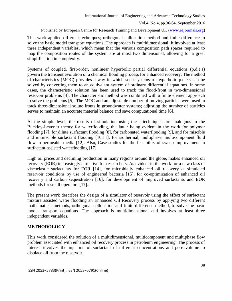
, , ,1 1,2iw i w x w i w y w i w i

CS C V f C V f C r i

t t x y

(15)

Fluid Phases





For incompressible phases, we can work in terms of volumes rather than moles. Thus, in Eqn.

12, j jC S and j jfJ = V so that:

0j

x j y j

SV f v f

t x y

(16)

Since there is no reactive fluid losses then eliminating of , carrying out the product

differentiation by the chain rule, multiplying the continuity equation (Eqn. 5) by jf , and

subtracting from Eqn.16, we obtain:

0 ,j j j

x y

S f fv v j o w

t x y

(17)

Again, multiplying Eqn.17 (for j w ) by ,i wC , Eqn.5 by ,w i wf C , and subtracting these from

Eqn.15 with application of the triple chain-rule leads to [18];

, , ,1 1,2

i w i w i wiw x w y w i

C C CCS v f v f r i

t t x y

(18)

The term ir represents the rate of loss of surfactant due to precipitation: for a one-to-one reaction

stoichiometry, 1 2r r . Since reaction occurs instantaneously at a sharp interface, this term may

be ignored away from the singular region of the interface.

Adsorption Model

It is possible to approximate the adsorption isotherm of a pure surfactant on a mineral oxide by

use of a simple model. At low concentration the adsorption obeys Henry‟s law, while above the

critical micelle concentration (CMC), the total adsorption remains constant. The Trogus

adsorption model [18, 20] is used in this work. The following assumptions are made:

(a) The composition and concentration of surfactant in the monomer and in the micelles can be

approximated by assuming that these are separate phases in thermodynamic equilibrium.

(b) Adsorption is a function of monomer composition only.

(c) Adsorption of an individual surfactant component is a linear function of its monomer

concentration (Henry‟s law), and is independent of micelle concentration and the other

component monomer concentrations.

Application of Finite Difference to Solution of Model Equations

First-order, finite-difference expressions for the spatial derivatives were substituted into the

hyperbolic chromatographic transport equations (Eq. 18), yielding 2 x m coupled ordinary

differential equations which may then be integrated simultaneously (also known as the

„numerical method of lines‟).





(19)

where i = 1,2 and h = 1,2,. .. m .

Eqn. 19 is the finite-difference form of Eqn.18 written for one spatial dimension , where ijm

are the adsorption coefficients , is dimensionless time ( injected volume/ pore volume), and

is dimensionless distance (pore volumes travelled). In two dimensions, the finite-difference

terms are multiplied by dimensionless velocities. The distortion of the solution in the direction

may be neglected by using a 4th

order Runge-Kutta method and a sufficiently small time step.

The above equation is now transformed to the original form of Eqns. 18 using the following

defined variables:

wiwi CC ,

'

, (20)

_

'_

' )1( ii CC (20)

'

,

_'

,

wj

iji

C

Cm

(21)

Again, recall that differentiation of a function of another function (chain rule) is of the form

x

u

u

y

x

y

(22)

Applying the chain rule above, Eqn. 19 becomes:

0),(),(

),(..1

'

,

'

,

'

,2

'

,2

_''

,1

'

,1

_''

,

hwihwi

hw

w

w

iw

w

iwi

w

CCf

C

C

CC

C

CCS

(24)

Eliminating the primes (') and bars (-) and introducing jim , terms yield

0,1,2

12

,1

11

w

w

ww

w

Cf

Cm

CmS

(25)

0,2,1

21

,2

22

w

w

ww

w

Cf

Cm

CmS

(26)

Applying the method of lines, a partial transformation to a difference equation, to the equations

above yield:

0)1,(),( ,1,1,2

12

,1

11

hhww

w

ww

w

CCf

Cm

CmS

(27)

2

, , 1, ,

1

, ,, 0

i w i wh hi w i ww ij w h

j

C CC Cs m f





0)1,(),( ,2,2,1

21

,2

22

hhww

w

ww

w

CCf

Cm

CmS

(28)

This can also be written as follows

0)1,(),(

),(

,1,1

,2

12

),(,1

11

hh

hh

ww

www

w CCfC

mC

mS

(29)

0)1,(),(

),(),(

,2,2

,1

21

,2

22

hh

hh

ww

www

w CCfC

mC

mS

(30)

Since we have a set of simultaneous ODE‟s, we will attempt to solve the equations

0)1,(),(

),(

,1,1

,2

12

),(,1

11

hh

hh

ww

www

w CCfC

mC

mS

(31)

0)1,(),(

),(),(

,2,2

,1

21

,2

22

hh

hh

ww

www

w CCfC

mC

mS

(32)

where

Substitution of these terms in Eqs. 31 and 32 yield:

0)1,(),(

),(

,1,1

,2

,2

1),(,1

,1

1

hh

hh

ww

ww

w

w

w

w CCfC

C

CC

C

CS

(33)

And

0)1,(),(

),(),(

,2,2

,1

,1

2,2

,2

2

hh

hh

ww

ww

w

w

w

w CCfC

C

CC

C

CS

(34)

These on simplification yield

w

w

w

w

C

Cm

C

Cm

C

Cm

C

Cm

,2

222

,1

221

,2

112

,1

111





02

02

0

0..

)1,(),(

)1,(),(

)1,(),(

)1,(),(

),(

,2,22),(,2

,1,11),(,1

,1,111),(,1

,1,1

,2

,2

1),(,1

,1

1),(,1

hh

h

hh

h

hh

h

hh

hhh

ww

ww

w

ww

ww

w

ww

ww

w

ww

ww

w

w

w

w

w

CCfCC

S

similarly

CCfCC

S

CCfCCC

S

CCfC

C

CC

C

CCS

(35)

(36)

From the Trogus model,

w

w

CkC

CkC

,222

,111

A final substitution results in the equation below:

0)2(

0)(

2

0)2(

02

0)(

2

)1,(),(

)1,(),(

)1,(),(

)1,(),(

)1,(),(

,2,2

,2

2

,2,2

,22),(,2

,1,1

,1

1

,1,1

,1

1

),(,1

,1,1

,11),(,1

hh

hh

h

hh

hh

h

hh

h

ww

ww

w

ww

www

w

ww

ww

w

ww

www

w

ww

www

w

CCfC

kS

CCfCkC

S

and

CCfC

kS

CCfC

kC

S

CCfCkC

S

(38)

Application of Orthogonal Collocation to Solution of Model Equations

Equation 24 can be written as:

0),(),(

),(21

'

,

'

,

_''

,

hwihwi

hw

iwi

w

CCf

CCS (39)

0),]([),]([

),(])1([

2][ 1,,

_

,

hwihwi

hw

iwi

w

CCf

CCS

(40)

(37)





0),(),(

),()1(21,,

_

,

hwihwi

hw

iwi

w

CCf

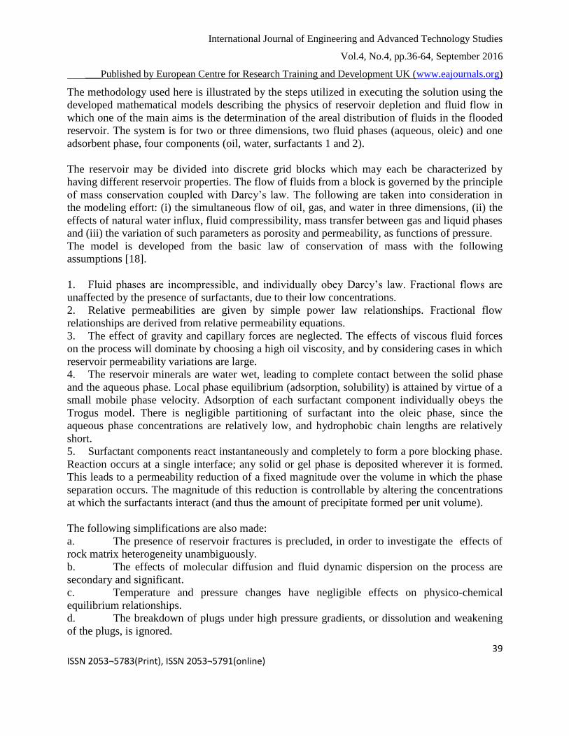
CCS (41)

Now, from the Trogus model,

wiii CC ,

_

(42)

0),(),(

),()(

)1(21,,,,

hwihwi

hw

wiiwi

w

CCf

CCS (43)

0),(),(

),()1(21,,,,

hwihwi

hw

wi

i

wi

w

CCf

CCS (44)

0),()1(2,,,

wi

hw

wi

i

wi

w

Cf

CCS (45)

0),()]1(2[,,

wi

hw

wi

iw

Cf

CS (46)

Let

w

iw

fB

SR

)]1(2[

The above equations now become:

0

CB

CR (47)

where C is a function of both ԑ (dimensionless distance) and τ (dimensionless time).

Using the method of orthogonal collocation, let C be approximated by the expression

1

1

)()(),(N

I

IJI XCC (48)

Equation 47 can now be expressed as follows:

0)()(1

1

N

I

IJI XCBC

R

(48)

0])()([1

1

N

I

IJI XCBC

R

(49)

0)(].)([1

1

I

N

I

IJ CXBC

R (50)

)( IJJI Xa

(51)

01

1

I

N

I

JI

J CaBC

R

(52)





01

1

I

N

I

JI

J CaR

BC

(53)

I

N

I

JI

J CaR

BC

1

1 (54)

For I = 1, 2, 3, 4… N+1

Therefore,

1144332211 ...

NJNJJJJ

J CaCaCaCaCaR

BC

(55)

Again J = 1, 2, 3, 4… N+1

Therefore the following system of ODE‟s can be generated

111414313212111

1 ...

NN CaCaCaCaCa

R

BC

112424323222121

2 ...

NN CaCaCaCaCa

R

BC

113434333232131

3 ...

NN CaCaCaCaCa

R

BC

114444343242141

4 ...

NN CaCaCaCaCa

R

BC

:

::

:

111414313212111

1 ...

NNNNNNN

N CaCaCaCaCaR

BC

(57)

In matrix form, we have the following expression:





1

211 12 13 14 1 1

21 22 23 24 2 1

331 3 1

41 4 14

11 12 1 1

1

... ... ... ... ...

:

:

: :

: ::

: ::

: ::

: ::

... ... ... ... ... ... ...:

N

N

N

N

N N N N

N

C

C a a a a a

a a a a aC

a a

a aC

B

R

a a a

C

1

2

3

4

1

( )

( )

( )

( )

( )N

C

C

C

C

C

(58)

Similarly, the following expression defines aJI [21,22].

)(

)(1

)(

)(

2

1

)1(

1

)1(

1

)1(

1

)2(

1

JN

IN

JI

IN

IN

JI

P

P

P

P

a

(59)

where

1)(

0)()(

)(2)()()(

)()()()(

1,...,3,2,1);()()(

0

)2(

0

)1(

0

)1(

1

)2(

1

)2(

1

)1(

1

)1(

1

P

PP

PPP

PPP

NJPP

JJJJ

JJJJ

JJJ

(60)

Recall that the elements of the matrix can be generated from the following Lagrange polynomial

For J = I

For I ≠ J





jijN

iN

ji

ijiN

iN

ij

ij

xP

xP

xx

xP

xP

dx

xdla

)(

)(1

)(

)(

2

1

)(

)1(

1

)1(

1

)1(

1

)2(

1

(61)

For i = j, the elements here refer to the leading diagonal of the matrix to be generated

For i ≠ j, the elements here refer to all other elements of the matrix

Also, the following recurrence relations are defined below.

)(2)()()(

)()()()(

)()()(

1)(

)1(

1

)2(

1

)2(

1

)1(

1

)1(

1

xPxPxxxP

xPxPxxxP

xPxxxP

xp

jjjj

jjjj

jjj

o

(62)

For j = 2, 3, 4, ..., N+1

The following substitutions and manipulations will now be made to redefine Eqn.61.

Substituting the recurrence relations into Eqn.61 yields:

jijjjjjj

ijijji

ji

ijijijji

ijijji

ij

xPxPxx

xPxPxx

xx

xPxPxx

xPxPxx

a

)()()(

)()()(1

)()()(

)(2)()(

2

1

1

)1(

1

1

)1(

1

1

)1(

1

)1(

1

)2(

1

(63)

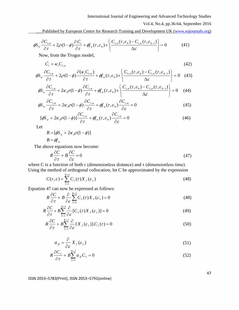
Now, some terms will be cancelled out.

Since j = i,

(xi – xj) = 0

and

(xj – xj)=0





jijj

ijijji

ji

ijij

ij

ij

xP

xPxPxx

xx

xP

xP

a

)(

)()()(1

)(

)(2

2

1

1

1

)1(

1

1

)1(

1

(64)

The above becomes:

jijj

ij

jijjji

ijji

ijij

ij

ij

xP

xP

xxxPxx

xPxx

xP

xP

a

)(

)(1

)()(

)()(

)(

)(

1

1

1

)1(

1

1

)1(

1

(65)

This becomes:

jijj

ij

jijj

ij

ijij

ij

ij

xP

xP

xxxP

xP

xP

xP

a

)(

)(1

)(

)(

)(

)(

1

1

1

)1(1

1

)1(1

(66)

Rewriting the above in terms of epsilon, (ε):

jijj

ij

jijj

ij

ijij

ij

ij

P

P

P

P

P

P

a

)(

)(1

)(

)(

)(

)(

1

1

1

)1(1

1

)1(1

(67)

The matrix now looks like this:

)(

)(

10

1

)1(

011

P

Pa





)(

)(1

)(

)(

21

11

2121

1

)1(

1

12

P

P

P

Pa

)(

)(1

)(

)(

32

12

2132

1

)1(

2

13

P

P

P

Pa

)(

)(1

)(

)(

10

20

1210

2

)1(

0

21

P

P

P

Pa

)(

)(

11

2

)1(

1

22

P

Pa

)(

)(1

)(

)(

32

22

3232

2

)1(

2

23

P

P

P

Pa

)(

)(1

)(

)(

10

30

1310

3

)1(

0

31

P

P

P

Pa

)(

)(1

)(

)(

21

31

2321

3

)1(

1

32

P

P

P

Pa

)(

)(

32

3

)1(

2

32

P

Pa

(68)

The recurrence relations below will again be used to evaluate the terms of the matrix.

1

(1) (1)

1 1

(1)

0

( ) 1

( ) ( ) ( )

( ) ( ) ( ) ( )

( ) 0

o

j j j

j j j j

p

P P

P P P

P

(69)

Let ԑ assume the range:

ԑ = [0:0.01:0.09]

where

ԑ1 = 0 (70)

ԑ2 = 0.01 (71)

ԑ3 = 0.02 (72)

RESULTS

The reservoir response, as predicted by the simulation on the basis of the theory of coherence, is

compared with the numerical predictions obtained using traditional finite difference method and

orthogonal collocation. The case studies are chosen to be both hypothetical and using of existing





Nigerian well data with simple representative of the important elements of the simulator. The

main objective of these case studies has been to demonstrate that the mathematical techniques of

orthogonal collocation, finite difference and coherent theory in the context of application of the

simulator can be used to obtain wave behaviour in a reservoir. A gradually increasing level of

complexity is introduced, representing a range of systems from aqueous phase flow, to surfactant

chromatography in two phase flow, to surfactant chromatography in two dimensional porous

medium. The initial and injected surfactant compositions corresponding to cases 1, and 2 are

shown in Table 5 in appendix. The rock and fluid properties are listed in Table 1, 2,3, 4 in

appendix. These were taken as uniform for convenience.

The two fluid phases consisted of a water phase and an oil phase, which, for convenience are

considered incompressible. The density of oil, the viscosity of oil, the salinity of water, and the

formation volume factor of oil and water are listed in Table 3.2 in appendix. All cases mentioned

above were run by using anionic sodium dodecyl sulfate (SDS) and cationic dodecyl pyridinium

chloride (DPC) as surfactants.

The system of equations is complete with the equations representing physical properties of the

fluids and the rock. From a physical-chemical point of view, there are three components - water,

petroleum and chemical. They are in fact, pseudo-components, since each one consists of several

pure components. Petroleum is a complex mixture of many hydrocarbons. Water is actually

brine, and contains dissolved salts. Finally, the chemical contains different kinds of surfactants.

These three pseudo-components are distributed between two phases –the oleic phase and the

aqueous phase. The chemical has an amphiphilic character. It makes the oleic phase at least

partially miscible with water or the aqueous phase at partially miscible with petroleum.

Interfacial tension depends on the surfactant partition between the two phases, and hence of

phase behaviour. Residual phase saturation decrease as interfacial tension decreases. Relative

permeability parameters depend on residual phase saturations. Phase viscosities are functions of

the volume fraction of the components in each fluid phase. Therefore, the success or failure of

surfactant flooding processes depends on phase behaviour. Phase behaviour influences all other

physical properties, and each of them, in turn influences oil recovery.

Results of Reservoir Prediction in an Aqueous Phase Chromatographic Flow in One

Dimension

Figure 1a is the result obtained for solving Equation 19 using the numerical technique for both

orthogonal collocation and finite difference. The graph is for the bed composition profile for one

dimensional aqueous-phase chromatography (case 1) at one half pore volume injected.

If a one-dimensional, adsorbing porous medium is initially equilibrated with an aqueous

composition C1 = 0.21, C2 = 0.181 ( concentrations normalized as moles in solution per m3 off

bed) and is then injected with a composition C1 = 0.17, C2 = 0.013 (Riemann-type problem: case





1, refer to Table 5 ), the composition upstream of this injected fluid and composition downstream

of the initial or previously injected fluid follows the slow “path” from the injected composition

to the junction with the “fast path” from the final composition, where it switches to this “fast”

path. In figure 1a, the profile C1 of finite difference (FD) shows a steady rise from C1 = 0.17 to

C1 = 0.21 and then attainecd a constant state. Also the profile C1 of the orthogonal collocation

(OC) increased steadily from C1 = 0.17 to C1 = 0.21 after which it started depressing from C1=

0.2 at distance 0.3 epsilon to C1 = 0.07 at distance 0.5 epsilon before rising back to attain a

constant state with the finite difference method. Similarly, the C2 of finite difference (FD)

increased steadily from C2 =0.017 to a constant state as for C1. The constant state is at C2 = 0.18.

The orthogonal collocation (OC) for C2 first moves at constant state before rising steadily to C2 =

0.18 and then declined from C2 = 0.18 to a minimum of C2 = 0.08 before rising to a constant

state. The profiles for finite difference (FD) and that of orhogonal collocation (OC) agree except

for the depressions of the orthogonal collocation profiles.

Figure 1b shows the result obtained for solving Equation 19 by using orthogonal collocation

(OC) and finite difference (FD) as the numerical technique. The graph is for the bed composition

profile for one dimensional aqueous phase chromatography for case 1 at one pore volume

injected.

In this case also, the adsorbing porous medium is initially equibrated with an aqueous

composition. C1 = 0.21, C2 = 0.181 ( concentrations normalized as moles in solution per m3 off

bed) and is then injected with a composition C1 = 0.17, C2 = 0.013 (Riemann-type problem: case

1,( refer to Table 5 ). The profile C1 of finite difference (FD) indicates rise in concentration from

C1 = 0.17 to 0.21 after which the concentration maintained a constant state. The profile of C1 of

the orthogonal collocation (OC) also rise from C1 = 0.17 to C1 = 0.21 but falls to 0.03 at distance

0.4 epsilon and then increased steadily to constant state as for C1 finite difference (FD). The C2

of finite difference increased steadily from C2 = 0.02 to attain constant state at 0.18. Also the

profile of C2 of the orthogonal collocation (OC) increase gradually from C2 = 0.02 to C1 = 0.18

at distance 0.2 epsilon for short constant state and then decline to C2 = 0.02 at distance 0.4

epsilon before rising back to reach constant state with the finite difference.

The bed composition profile for one dimensional aqueous phase chromatography for case 1 at

two pore volume injected is shown in Figure 1c. This is the result obtained for solving Equation

19 by using numerical technique for both the orthogonal collocation (OC) and finite difference

(FD). The adsorbing porous medium is initially equibrated with an aqueous composition. C1 =

0.21, C2 = 0.181 (concentrations normalized as moles in solution per m3 off bed) and is then

injected with a composition C1 = 0.17, C2 = 0.013 (Riemann-type problem: case 1,( refer to

Table 5 in appendix) ), The profile C1 of finite difference (FD) and the profile C1 of orthogonal

collocation (OC) indicate that there is steady increase from C1 = 0.17 to C1 = 0.21 at distance 0.1

epsilon and then attained a constant state for both profiles. Similarly, the profile C2 of finite

difference (FD) shows a steady rise from C2 = 0.02 to C2 = 0.18 and then maintained a constant

state. Also, the profile C2 for orthogonal collocation (OC), follows the same pattern, which

indicate an increase from C2 = 0.02 to C2 = 0.18 and then attained a constant state. The

orthogonal collocation (OC) profiles match the finite difference (FD) profiles.





0 0.1 0.2 0.3 0.4 0.5 0.6 0.7 0.8 0.9 10

0.05

0.1

0.15

0.2

0.25

dimensionless distance, epsilon

C1,C

2,C

C1,C

C2(m

ole

s in s

oln

/m3 b

ed)

CC1-FD

CC2-FD

CC1-OC

CC2-OC





FIGURE 1a. CASE 1 C1,C2,CC1,CC2 vs epsilon at τ = 0.5. Bed composition profile for one-

dimensional aqueous-phase chromatography; case 1, at one-half pore volume injected. The plots

are for two methods: Orthogonal collocation (OC), and finite difference (FD).

FIGURE 1b CASE 1 C1,C2, CC1,CC2 vs epsilon at τ = 1.0. Bed composition profile for one-

dimensional aqueous-phase chromatography; case 1, at one pore volume injected. The plots are

for two methods: Orthogonal collocation (OC), and finite difference (FD).

0 0.1 0.2 0.3 0.4 0.5 0.6 0.7 0.8 0.9 10

0.05

0.1

0.15

0.2

0.25


C1,C

2,C

C1,C

C2(m

ole

s in s

oln

/m3 b

ed)

CC1-FD

CC2-FD

CC1-OC

CC2-OC





FIGURE 1c CASE 1 C1,C2 CC1,CC2 vs epsilon at τ = 2.0. Bed composition profile for one-

dimensional aqueous-phase chromatography; case 1, at two pore volumes injected. The plots are


Figure 2a shows the bed concentration profiles for one dimensional aqueous phase

chromatography for case 2 at one-half pore volume injected in the adsorbing porous medium

initially devoid of surfactant and then injected with a mixture C1 = 0.042, C2 = 0.115

(Riemann-type problem: case 2 ( refer to Table 5 ), with the numerical result obtained for solving

Equation 19 by using orthogonal collocation (OC) and finite difference (FD) as the numerical

technique.The profile C1 of finite difference (FD) indicates a steady fall from in concentration

from C1 = 0.04 to a constant state of zero. The profile of C1 of the orthogonal collocation (OC)

falls steadily from C1 = 0.04 but however oscillates between 0.01 and 0.04 jumping to its

injection value before attaining constant state with the finite difference (FD). Similarly the C2 of

finite difference (FD) decreased steadily from C2 = 0.119 to a constant state as for C1. Also the

profile C2 of orthogonal collocation (OC) decreases steadily from C2 = 0.119 but however gives

a more pronounced oscillation from C2 = 0.02 and C2 = 0.119 jumping to its injection value

before attaining constant state with the finite difference(FD).

0 0.1 0.2 0.3 0.4 0.5 0.6 0.7 0.8 0.9 10

0.05

0.1

0.15

0.2

0.25


C1,C

2,C

C1,C

C2(m

ole

s in s

oln

/m3 b

ed)

CC1-FD

CC2-FD

CC1-OC

CC2-OC





Figures 2b and 2c compare the bed concentration profiles expected at one and two pore volume

injected with a mixture C1 = 0.042, C2 = 0.115 in the adsorbing porous medium initially devoid

of surfactant (Riemann-type problem: case 2,( refer to Table 5)). The graph shows the results

obtained using the numerical technique; finite difference (FD) and orthogonal collocation (OC)

In figure 2b, the profile C1 of finite difference (FD) shows steady decline from from C1 = 0.04 to

a constant state. Also the C1 of orthogponal collocation falls steadily from C1= 0.04 to a constant

state as for finite difference (FD). The profile C2 of finite difference decreased steadily from C2 =

0.119 to a constant state as for C1. Similarly, the C2 of orthogonal collocation (OC) falls steadily

from C2 = 0.119 to a constant state.

In figure 2c, the profiles C1 of orthogonal collocation (OC) follow the same pattern as that in

figure 2b. Similarly, the profiles C2 of finite difference (FD) and orthogonal collocation (OC)

have the same pattern as in figure 2b

FIGURE 2a CASE 2. C1,C2, CC1,CC2 vs epsilon at τ = 0.5. Bed composition profile for one-

dimensional aqueous-phase chromatography; case 2, at one-half pore volume injected. The plots

are for two methods: Orthogonal collocation (OC), and finite difference (FD).

0 0.1 0.2 0.3 0.4 0.5 0.6 0.7 0.8 0.9 10

0.02

0.04

0.06

0.08

0.1

0.12


C1,C

2,C

C1,C

C2(m

ole

s in s

oln

/m3 b

ed)

CC1-FD

CC2-FD

CC1-OC

CC2-OC





FIGURE 2b.CASE 2 C1,C2, CC1,CC2 vs epsilon at τ = 1.0. Bed composition profile for one-

dimensional aqueous-phase chromatography; case 2, at one pore volume injected. The plots are


FIGURE 2c CASE 2. C1,C2, CC1,CC2 vs epsilon at τ = 2.0. Bed composition profile for one-

dimensional aqueous-phase chromatography; case 2, at two pore volumes injected. The plots are

for two methods: Orthogonal collocation (OC) and finite difference (FD).

0 0.1 0.2 0.3 0.4 0.5 0.6 0.7 0.8 0.9 10

0.02

0.04

0.06

0.08

0.1

0.12


C1,

C2,

CC

1,C

C2(

mol

es in

sol

n/m

3 bed

)

CC1-FD

CC2-FD

CC1-OC

CC2-OC

0 0.1 0.2 0.3 0.4 0.5 0.6 0.7 0.8 0.9 10

0.02

0.04

0.06

0.08

0.1

0.12


C1,

C2,

CC

1,C

C2(

mol

es in

sol

n/m

3 bed

)

CC1-FD

CC2-FD

CC1-OC

CC2-OC





DISCUSSION OF RESULTS

The prediction of the appropriate surfactant concentration necessary for the required enhanced

oil recovery from reservoirs and the basic physical principle employed by the simulator is that of

mass conservation. Usually those quantities are conserved at stock tank conditions and related to

reservoir fluid quantities through the pressure dependent parameters. The profiles of two cases

1and 2, one dimensional aqueous phase chromatography and two-phase chromatography for one,

one-half, and two pore volume injected were developed using simulated solutions to model

equations. These equations are solved by finite difference (FD) and orthogonal collocation (OC).

The use of these methods permit the determination of the relative efficiency of the methods and

how well they predicts the complex characteristics of the enhanced oil recovery process.

Injecting a mixture of low concentration aqueous surfactant composition into adsorbing porous

medium that is initially injected with high concentration aqueous surfactant composition. This

variation may exist in the initial profile or be generated by injection. The initial fluid or

previously injected fluid has the composition downstream of the change in amount while the

newly injected fluid has the composition upstream of the original variation. The composition

route along the bed follows the slow path from the injected composition and then switches to the

fast path which leads to the previously injected composition. The route passes along paths and

follows the paths in the sequence of increasing wave velocities.

Injecting a mixture of an aqueous composition into a porous medium, initially devoid of

surfactant, the expected composition is a self-sharpening shock wave. The steepness in all the

profiles generated by finite difference (FD), and orthogonal collocation (OC), confirms the self

sharpening behaviour. It may be noted in all cases of these natures the waves trajectories

gradually fall, as a result of a gradual increase in the associated eigenvalues of the waves as

salinity increases. The consequence of this steepening is that the flows are sharpening, so that

they break through both earlier and over a smaller injected volume. For the dependent variables

such as component concentration, common velocity exists at each point in the wave, and the

associated composition route remains unchanged and the same during relative shifts of waves

associated with other dependent variable waves as shown in the methods. This is in agreement

with other work [3].

The complexities could not have been detected by using only the coherent technique [18]. This is

a major accomplishment of this work. Not only was the discontinuities discovered by this work,

it also provides an insight into the complex behaviour of enhanced oil recovery process.

CONCLUSIONS

The applicability of the simulator for the solution of the model equations of multiphase,

multicomponent flow and transport in a reservoir has been demonstrated using orthogonal

collocation solution and finite difference. The results of the orthogonal collocation solution were

compared with those of finite difference. The results obtained using this methodology revealed





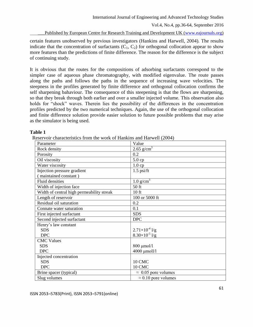
certain features unobserved by previous investigators (Hankins and Harwell, 2004). The results

indicate that the concentration of surfactants (C1, C2) for orthogonal collocation appear to show

more features than the predictions of finite difference. The reason for the difference is the subject

of continuing study.

It is obvious that the routes for the compositions of adsorbing surfactants correspond to the

simpler case of aqueous phase chromatography, with modified eigenvalue. The route passes

along the paths and follows the paths in the sequence of increasing wave velocities. The

steepness in the profiles generated by finite difference and orthogonal collocation confirms the

self sharpening bahaviour. The consequence of this steepening is that the flows are sharpening,

so that they break through both earlier and over a smaller injected volume. This observation also

holds for “shock” waves. Therein lies the possibility of the differences in the concentration

profiles predicted by the two numerical techniques. Again, the use of the orthogonal collocation

and finite difference solution provide easier solution to future possible problems that may arise

as the simulator is being used.

Table 1

Reservoir characteristics from the work of Hankins and Harwell (2004) Parameter Value

Rock density 2.65 g/cm3

Porosity 0.2

Oil viscosity 5.0 cp

Water viscosity 1.0 cp

Injection pressure gradient

( maintained constant )

1.5 psi/ft

Fluid densities 1.0 g/cm3

Width of injection face 50 ft

Width of central high permeability streak 10 ft

Length of reservoir 100 or 5000 ft

Residual oil saturation 0.2

Connate water saturation 0.1

First injected surfactant SDS

Second injected surfactant DPC

Henry‟s law constant

SDS

DPC

2.71×10-4

l/g

8.30×10-5

l/g

CMC Values

SDS

DPC

800 μmol/l

4000 μmoll/l

Injected concentration

SDS

DPC

10 CMC

10 CMC

Brine spacer (typical) ≈ 0.05 pore volumes

Slug volumes ≈ 0.10 pore volumes





TABLE 2

Reservoir Characteristics used for the Simulation work by Oyedeko (2012) Parameter Value

Rock density 2.65 g/cm3

Porosity 0.2

Oil viscosity 0.40 cp

Water viscosity 0.30 cp

Injection pressure gradient

( maintained constant )

1.5 psi/ft

Fluid densities 1.0 g/cm3

Width of injection face 50 ft

Width of central high permeability streak 10 ft

Length of reservoir 100 or 5000 ft

Residual oil saturation 0.2

Connate water saturation 0.2

First injected surfactant SDS

Second injected surfactant DPC

Henry‟s law constant

SDS

DPC

2.71×10-4

l/g

8.30×10-5

l/g

CMC Values

SDS

DPC

800 μmol/l

4000 μmoll/l

Injected concentration

SDS

DPC

10 CMC

10 CMC

Brine spacer (typical) ≈ 0.05 pore volumes

Slug volumes ≈ 0.10 pore volumes

Table 3

Parameter values used in Trogus adsorption model for verification runs Parameter Value

Pure component CMCs C1*=1.0 mol/m3

C2*=0.35 mol/m3

Phase separation model parameter θ=1.8

Henry‟s law constants for adsorption

,i i i wC k C

(,i wC = aqueous monomer concentration)

k1 =0.21×10-3

m3/kg

k2= 0.80×10-3

m3/kg

Henry‟s law constant for oleic partitioning , ,i o i i wC q C

(,i wC = aqueous monomer concentration)

q1=7.1

q2=1.3

Adsorbent properties ρs =2.1× 10+3

m3/kg

∅ =0.2





Table 4

Additional Reservoir Parameters for the coherence work by Hankin and Harwell (2004)

Model designation A B

Grid points in the horizontal direction ( m+1) 21 21

Grid points in the vertical direction (n+1) 11 21

Coherent waves of water saturation 28 28

Initial number of points per coherent wave

Water

Surfactant

41

81

41

81

Maximum number of points required per coherent

wave

≈ 300 ≈300

Average time step size (days)

Short reservoir (100 ft)

200 mD streak

1000 mD streak

Long reservoir (5000ft)

200 mD streak

1000 mD sreak

3.47

0.69

174.0

34.7

3.47

0.69

174.0

34.7

Typical number of time steps required to inject first

pore volume

Short reservoir

Long reservoir

33

75

33

75

Table 5

Conditions for case studies of surfactant chromatography[18].

Case Injected

composition:

CC1(mol/m3 bed)

Injected

composition:

CC2(mol/m3bed)

Initial

composition:

C1(mol/m3bed)

Initial

composition:

C2(mol/m3bed)

1 0.17 0.013 0.21 0.181

2 0.042 0.115 0 0

3 0.66 0.875 0.35 0.15

REFERENCES

[1]. S.M. Bidner, and G.B. “Savioli, On the numerical modeling for surfactant flooding of oil

Reservoirs.” Mecanica Computational vol.xxl, pp556-585, 2002.

[2]. S.C. Ayirala, “Surfactant-induced Relative Permeability Modifications For Oil Recovery

Enhancement”, LSU, Louisiana, 2002.

[3]. F.G. Helfferich. “Theory of Multicomponent, Multiphase Displacement in Porous Media.” Soc.

Pet. Eng. J., 21: 51-62, 1981.

[4]. J. Glimm, B. Lindquist, O.A. McBryan, B. Plohr, B. and S. Yaniv. “Front Tracking for





Petroleum Reservoir Simulation.” Paper SPE 12238 Presented at the seventh SPE Symposium on

Reservoir Simulation, San Francisco, Society of Petroleum Engineers of AIME, Dallas, Texas

(USA). Nov. 16-18, 1983.

[5]. R.E. Ewing, T.F. Russel and M.F. Wheeler. “Simulation of Miscible Displacement using Mixed

Methods and a Modified Method of Characteristics.” Paper SPE 12241 Presented at the seventh

SPE Symposium on Reservoir Simulation, San Francisco, Society of Petroleum Engineers of AIME,

Dallas, Texas (USA). Nov. 16-18, 1983.

[6]. C. Zheng. “Extension of the Method of Characteristics for Simulation of Solute Transport in 3

Dimensions.” Ground Water, 31(3): 456-465, 1993.

[7]. J.R. Patton, K.H. Coats and G.T. Colegrove. “Prediction of Polymer Flood Performance.”

Soc.Pet. Eng., 11: 72-84, 1971.

[8]. F.J. Fayers and R.I. Perrine. “Mathematical Description of Detergent Flooding in Oil

Reservoirs.” Petroleum Trans. AIME, 216: 277-283, 1959.

[9]. E.L. Claridge and P.I. Bondor. (1974). “A Graphical Method for Calculating Linear

Displacement with Mass Transfer and Continuously Changing Mobilities.” Soc. Pet. Eng. J., 14;

609-618, 1974.

[10]. R.G. Larson.” The Influence of Phase Behaviour on Surfactant Flooding.” Soc. Pet. Eng. J.,

19: 411-422, 1979.

[11]. G.I. Hirasaki. “Application of the Theory of Multicomponent, Multiphase Displacement to

Three-Component, Two-Phase Surfactant Flooding.” Soc. Pet. Eng. J., 21: 191-204, 1981.

[12]. G.A. Pope, G.F. Carey and K. Sepehrnoori. “Isothermal, Multiphase, Multicomponent Fluid

Flow in Permeable Media. Part II: Numerical Techniques and Solution.” In Situ, 1984, 8(1): 1-40

[13] N.P. Hankins and J.H. Harwell. “Case Studies for the Feasibility of Sweep Improvement in

Surfactant-assisted Waterflooding.” J. Pet. Sci. Eng., 17: 41-62, 1997.

[14]. L. Siggel, M. Santa, M. Hansch, M. Nowak, M. Ranft, H. Weiss, D. Hajnal, E. Schreiner, G.

Oetter, G. and J. Tinsley. “A New Class of Viscoelastic Surfactants for Enhanced Oil Recovery

BASFSE SPE Improved Oil Recovery Symposium,”, Tulsa, Oklahoma, USA. 14-18 April, 2001.

[15]. Y. Xu, and M. Lu. “Microbially Enhanced Oil Recovery at Simulated Reservoir Conditions

by Use of Engineered Bacteria.” J. Petr. Sci. Eng., 78(2): 233-238, 2001.

[16]. A. Leach, A. and C.F. Mason. “Co-optimization of Enhanced Oil Recovery and Carbon

Sequestration.” J. Resource and Energy Economics, 33(4): 893-912, 2011.

[17]. J.H. Harwell. “Enhanced Oil Recovery Made Simple.” J. Petr. Technol., 60(10): 42-43,

2012.

[18] N.P. Hankins. and J.H. “Harwell. Application of Coherence Theory to a Reservoir

Enhanced Oil Recovery Simulator.” J. Pet. Sci. Eng., 42: 29-55, 2004.

[19]. K.F. Oyedeko. “Design and Development of a Simulator for a Reservoir Enhanced Oil

Recovery Process.” PhD Dissertation, Lagos State University, Ojo, Lagos, Nigeria, 2014.

[20]. F.J. Trogus, R.S. Schecchter, G.A. Pope and W.H. Wade. “New Interpretation of

Adsorption Maxima and Minima.” J. Colloid Interface Sci., 70(3): 293-305, 1979.

[21] J.V. Villadsen and W.E. Stewart. “Solution of Boundary Value Problems by Orthogonal

Collocation.” Chem. Eng. Sci., 22: 1483-1501, 1967.

[22] J.V. Villadsen and W.E. Stewart. “Solution of Boundary Value Problems by Orthogonal

Collocation.” Chem. Eng. Sci., 23: 1515, 1968.

http://academic.research.microsoft.com/Author/21447279/yaohui-xu

http://academic.research.microsoft.com/Author/21907865/mang-lu

http://academic.research.microsoft.com/Journal/6436/j-pet-sci-engineering-journal-of-petroleum-science-and-engineering

http://academic.research.microsoft.com/Author/5820784/andrew-j-leach

http://academic.research.microsoft.com/Author/22644663/charles-f-mason



http://academic.research.microsoft.com/Journal/5010/resour-energy-econ-resource-and-energy-economics

Date post:	08-Mar-2018
Category:	Documents
Upload:	truongthuan
View:	219 times
Download:	2 times

DESIGN OF A SIMULATOR OF A RESERVOIR · PDF fileInternational Journal of Engineering and...

Documents