Design of a SystemView Simulation of a Stepped Frequency Continuous Wave Ground Penetrating Radar Prepared By Andile Mngadi Final year Electrical Engineering Student University of Cape Town This thesis is submitted to the Department of Electrical Engineering, University of Cape Town, in partial fulfilment of the requirements for the degree of Bachelor of Science in Engineering. Cape Town, October 2004 25th October 2004 Document No: rrsg:00
Transcript
Design of a SystemView Simulation of a Stepped
Frequency Continuous Wave Ground Penetrating
Radar
Prepared By
Andile Mngadi
Final year Electrical Engineering Student
University of Cape Town
This thesis is submitted to the Department of Electrical Engineering,
University of Cape Town, in partial fulfilment of the requirements
for the degree of Bachelor of Science in Engineering.
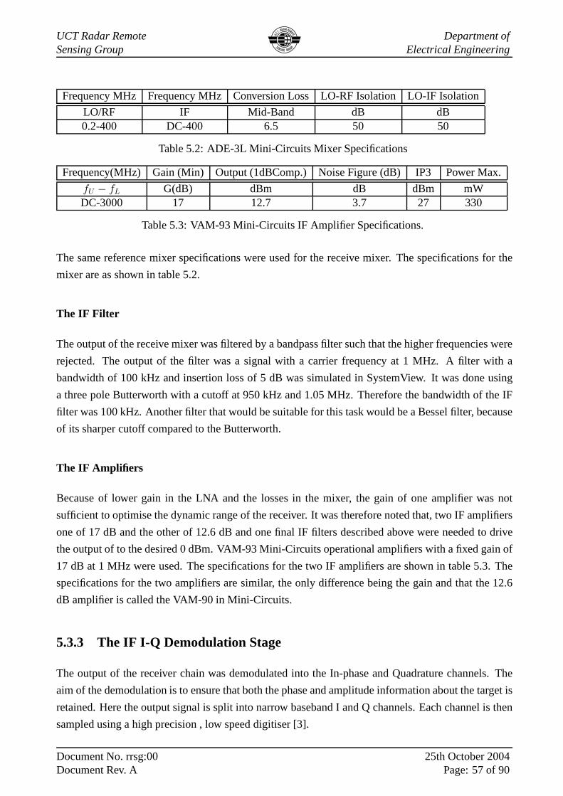
Frequency(MHz) Gain (Min) Output (1dBComp.) Noise Figure (dB) IP3 Power Max.
fU − fL G(dB) dBm dB dBm mWDC-3000 17 12.7 3.7 27 330
Table 5.3: VAM-93 Mini-Circuits IF Amplifier Specifications.
The same reference mixer specifications were used for the receive mixer. The specifications for the
mixer are as shown in table 5.2.
The IF Filter
The output of the receive mixer was filtered by a bandpass filter such that the higher frequencies were
rejected. The output of the filter was a signal with a carrier frequency at 1 MHz. A filter with a
bandwidth of 100 kHz and insertion loss of 5 dB was simulated in SystemView. It was done using
a three pole Butterworth with a cutoff at 950 kHz and 1.05 MHz.Therefore the bandwidth of the IF
filter was 100 kHz. Another filter that would be suitable for this task would be a Bessel filter, because
of its sharper cutoff compared to the Butterworth.
The IF Amplifiers
Because of lower gain in the LNA and the losses in the mixer, the gain of one amplifier was not
sufficient to optimise the dynamic range of the receiver. It was therefore noted that, two IF amplifiers
one of 17 dB and the other of 12.6 dB and one final IF filters described above were needed to drive
the output of to the desired 0 dBm. VAM-93 Mini-Circuits operational amplifiers with a fixed gain of
17 dB at 1 MHz were used. The specifications for the two IF amplifiers are shown in table 5.3. The
specifications for the two amplifiers are similar, the only difference being the gain and that the 12.6
dB amplifier is called the VAM-90 in Mini-Circuits.
5.3.3 The IF I-Q Demodulation Stage
The output of the receiver chain was demodulated into the In-phase and Quadrature channels. The
aim of the demodulation is to ensure that both the phase and amplitude information about the target is
retained. Here the output signal is split into narrow baseband I and Q channels. Each channel is then
sampled using a high precision , low speed digitiser [3].
Document No. rrsg:00Document Rev. A
25th October 2004Page: 57 of 90
UCT Radar RemoteSensing Group
Department ofElectrical Engineering
So
Spitter L.O @ 1MHz
90
0
Spitter90
o
Resampler
Resampler Quantizer
QuantizerI signal
Q signal Q
I
LPF
LPF
IFcos(w t )cos(wt)
Figure 5.4: Diagram showing how the I-Q Demodulation in SystemView was achieved.
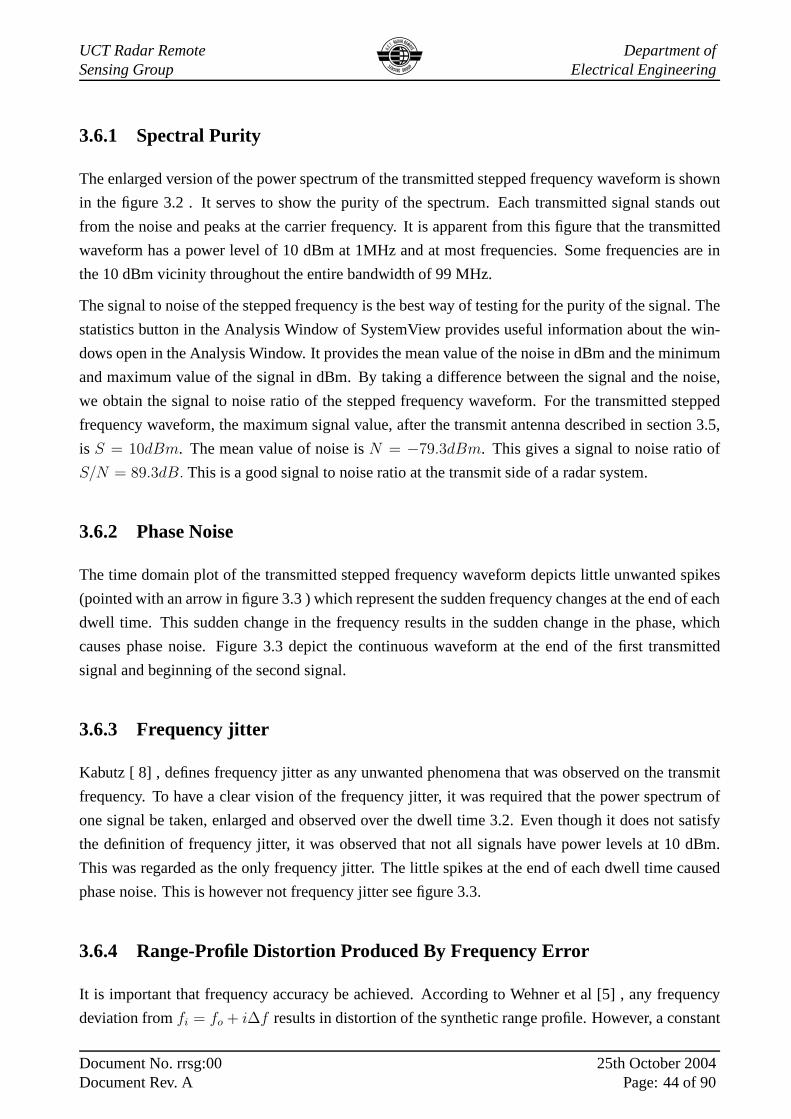
5.3.3.1 Simulation of the Demodulation Stage
The output of the receiver chain was demodulated into the In-phase and Quadrature channels as shown
in figure 5.4 . SystemView does not have a I-Q demodulator, thus a group of tokens were assembled
together to simulate the demodulator. The final output IF signal from the IF filter, was split into two
similar signals using a SystemView splitter PSplitter-2. Because the output signal is at 1 MHz, the
local oscillator shown in figure 5.3 was used for demodulation. The one signal was demodulated
with a local oscillator signal, that iscos(ωIF tn) , to produce the In-phase. The other signal was
demodulated using the900 phase shifted local oscillator signal, that issin(ωIF tn) , to produce the
Quadrature signal. This means that the reference of the local oscillator was split into two signal, one
of them shifted by900. The two I and Q signals were lowpass filtered using a 3 pole Butterworth IIR
filter with a cutoff frequnecy of 1.05 MHz. The I and Q time representation before the quantisation
of the signals is shown in figure 5.5 for the first three frequencies.
5.3.3.2 Analogue to Digital Conversion or Quantisation
The analogue to digital conversion was done using a quantiser. In SystemView a quantiser performs
the same task as the analogue to digital converter. But is simpler because the quantiser does not need
clock synchronisation. The I and Q signals have a quoted minimum signal value of -2.686 mV and
-2.441 mV respectively. And a quoted maximum value of 5.371 mV and 18.42 mV respectively. The
I and Q signals have a quoted mean noise value of7.201 × 10−2mV and4.682mV respectively. A
14 bit quantiser with a voltage span of 2 V was used. The stepsize of the quantiser therefore was
a = Vspan
214 = 122 × 10−3mV and the number of quantisation levels is214 − 1 = 16383 . To be able
to do signal integration of the system, the thermal noise must be greater thana/2 . The minimum
noise value was7.201 × 10−2mV which is greater than61.035µV . When no signal was present the
Document No. rrsg:00Document Rev. A
25th October 2004Page: 58 of 90
UCT Radar RemoteSensing Group
Department ofElectrical Engineering
(a)
(b)
Figure 5.5: The In-phase and Quadrature time domain plots before the quantisation or digitisation.
Document No. rrsg:00Document Rev. A
25th October 2004Page: 59 of 90
UCT Radar RemoteSensing Group
Department ofElectrical Engineering
noise toggled the quantiser and it sampled even when no signal was present. The output data values
of the quantiser were then taken to Matlab for further signalprocessing. A SystemView diagram of
the completed receiver is shown in Appendix C. The range profile plots of Matlab are also shown in
Appendix C.
5.4 Receiver Performance
The performance of the receiver system was based on the output SNR, the receiver dynamic range,
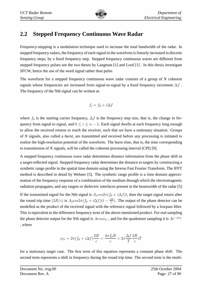
the MDS. The purity of the power spectrum of the output signalwas also observed. Figure 5.6 show
the output spectrum of the receiver given that the transmitted signal was 10 dBm and the medium was
10 dB. The power of the output signal was observed to be -7 dBm.The I and Q plots show an average
noise of 7.201x10⁻² [mV] as as input to the quantiser. Thus the toggles the quantiser to sample even
when no input signal is present.
5.4.1 Signal to Noise Ratio
.
5.4.2 Noise Figure
When the receiver simulation was designed above, it was found that more gain was needed in the
IF stage in order to optimise the dynamic range of the receiver. It was therefore noted that, two
IF amplifiers one of 17 dB and the other of 12.6 dB and one final IFfilters described above were
needed to drive the output of to the desired 0 dBm. The input signal to noise ratio at the input of the
receiver was calculated atSi
Ni= 89.54dB. From the above section the output signal to noise ratio is
S0
N0
= 126.89dB with the noise atN0 = −126.9dBm, all being system values. Thus the noise figure isSi/Ni
S0/N0= −37.356dB. This value of the noise figure does not make sense. The longhand-calculation
of the noise figure gives
F = F1 +F2 − 1
G1+
F3 − 1
G1G2+ ...... = 5dB
whereF1 = 2.7dB andG1 = 16dB. The long hand calculation gives a noise figure better thanthe
specifications requirements. This is the genuine noise figure of the system for the following reason.
The writer found that the dBm values of SystemView are in essence dB. Because of that error in
the SystemView analysis window, the successive mean, minimum and maximum values for the noise
Document No. rrsg:00Document Rev. A
25th October 2004Page: 60 of 90
UCT Radar RemoteSensing Group
Department ofElectrical Engineering
(a)
Figure 5.6: Power Spectra at the receiver output.
Document No. rrsg:00Document Rev. A
25th October 2004Page: 61 of 90
UCT Radar RemoteSensing Group
Department ofElectrical Engineering
and signal are circumstantially erroneous. However, the writer decided to use the SystemView noise
figure value for the rest of the receiver analysis for simplicity reasons.
5.4.3 Compression and Third-Order Intermodulation
The power levels that exceed the 1 dB compression pointP1 of an amplifier will cause harmonic
distortion and power levels in excess of the third order intercept pointP3 will cause intermodulation
distortion. Therefore it is important to track the power levels through the stages of the receiver to
ensure thatP1 andP3 are not exceeded. This was conveniently done with a graph of the form shown
in figure 5.7. It was found that theP1 andP3 of the amplifiers and mixer were not exceeded as shown
in the figure 5.7.
The third-order intercept pointP3 was taken as the smallest of all the components in the system since
that is the minimumP3 that should not be exceeded by the signal. Similar analogy was used forP1
. Thus the values forP1 andP3 respectively are 12.7 and 27 dBm. TheP3 values are not shown in
figure 5.7, because they are well above theP1. If P1 cannot be exceed,P3 cannot be exceeded as well.
5.4.4 Receiver Dynamic Range
The linear dynamic range of the system was calculated at
DRl = P1 − N0 = 12.7 − (−126.9) = 139.6dB
The spurious free dynamic range was calculated at
DRf =2
3(P3 − N0 − SNR) =
2
3(27 − (−126.9) − 119.9) = 22.67dB
5.5 Summary
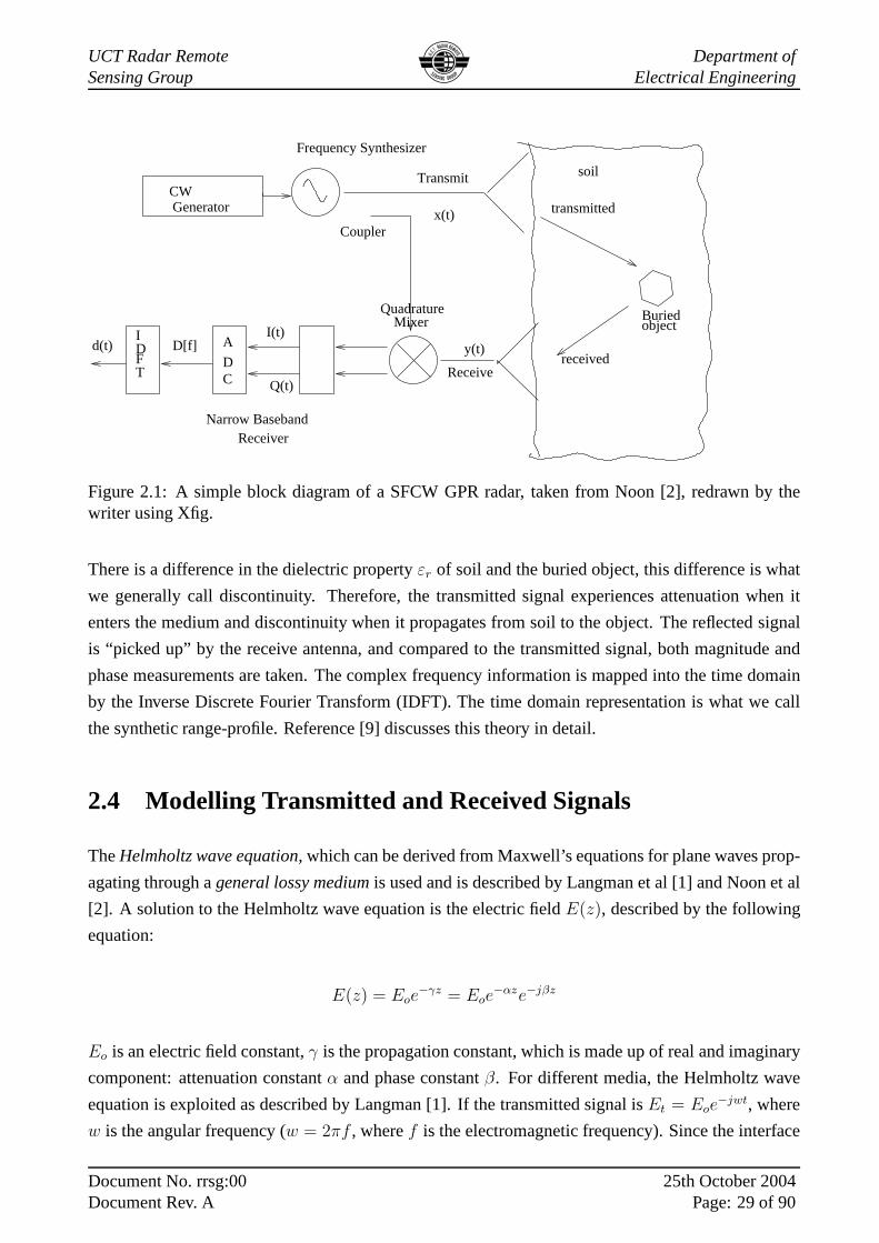
This chapter can be summarised as follows. A heterodyne architecture was chosen because the homo-
dyne architecture has limitations that the heterodyne easily overcome. Thus the receiver simulation
was a single conversion heterodyne with three stages. The first stage was the RF stage with a preselect
filter of 100MHz bandwith and a Mini-Circuit GALI-52 LNA RF amplifier. The function of thepre-
selectfilter is to reject out-of-band interference, which is particularly important for preventing strong
interference signals from saturating the RF amplifier or mixer.The second stage, the IF stage, the
bandpass filtered output of the low-noise amplifier is down-converted to an intermediate frequency.
Document No. rrsg:00Document Rev. A
25th October 2004Page: 62 of 90
UCT Radar RemoteSensing Group
Department ofElectrical Engineering
LO @ 1MHz
Reference of Tx
1 − 100MHz
Rx
LNA
100kHz
IF Filter IF Amp
1MHz
Mixer
100MHz G=16dB
L =6.5dB
Mixer
L = 6.5dB
100kHz
So To
Demodulation
Antenna
Receive
PreselectBPF BPF
20
10
0
10
20
30
40
50
60
70
80
90
100
110
120
130
140
Pow
er−
level
dB
m
−
−
−
−
−
−
−
−
−
−
−
−
−
−
Input Signal
G=29.6dBL = 5 dB
L = 5 dB L = 1 dB
−27.06
LNA P1
(output)15.5
IF AMP P1(output)12.7
Noise
Figure 5.7: Diagram of noise and signal at consecutive stages of the receiver.
Document No. rrsg:00Document Rev. A
25th October 2004Page: 63 of 90
UCT Radar RemoteSensing Group
Department ofElectrical Engineering
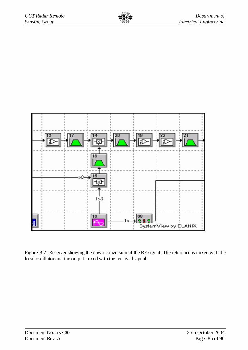
A reference of the transmitted frequency is mixed with the local oscillator frequencyfL0 . This RF
mixing signal is then used to drive the receiver mixer. Thus the received frequencyfRx is mixed by
fTx ± fLO , the transmit frequency offset by the IF frequency. The output of the receiver mixer will
consist of the two difference terms added at the IF and the twosum terms which are rejected by the
IF filter. The two mixers used in the simulation were Mini-Circuit ADE-3L mixers with a conversion
loss of 6.5 dB. The bandwidth of the IF filter was 100 kHz. This filter was designed in SystemView
using a three pole Butterworth filter with a cutoff at 950 kHz and 1.05 MHz. The output of the filter
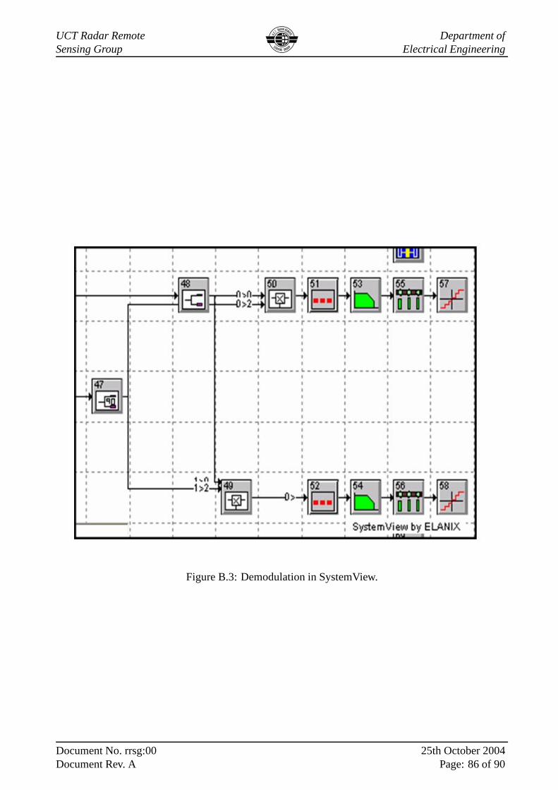
was a signal with a 1 MHz carrier frequency. The third stage was the demodulation stage where the 1
MHz signal was demodulated into In-phase and Quadrature components using the local oscillator sig-
nal. The 1 MHz was split into two equal signals using SystemView’s power splitter. The two signals
were then mixed with local oscillator at 1 MHz to baseband using ADE-3L mixers. The basebanded
signals were then digitised using high precision and low speed 14 bit quantisers. The data was kept
into a file for further analysis in Matlab. The performance ofthe receiver was then conducted based
on the SNR, the third-order intermodulation and the dynamicrange.
Document No. rrsg:00Document Rev. A
25th October 2004Page: 64 of 90
UCT Radar RemoteSensing Group
Department ofElectrical Engineering
Chapter 6
The Comparison of SFCW GPR to Impulse
GPR
6.1 Introduction
In this chapter the results of the comparison simulated SFCWGPR system will be presented. In
chapters 3, 4, and 5 the performance of the transmitter, the medium and the receiver was discussed
and results with regard their performance were shown. For the transmitter, its performance is inves-
tigated in section 3.6. The propagation medium performanceis shown in section 4.4. The receiver
performance is tested section 5.4. Therefore those resultswill not be repeated in this chapter.
For comparison purposes, both the Impulse and SFGPR radar systems were modified to have the
same propagation medium characteristics. Further modification that was made to the existing SFCW
system is described in section 6.2. The modified SFCW GPR system performance is discussed in
section 6.3. A summary of how range profiling and what it meansis included followed by range
profiles of the two systems in section 6.5. The last section briefly summarise the performance of the
SFCW GPR compared to the Impulse GPR.
6.2 Modifying the existing system
When the SFGPR system performance was compared to the Impulse radar system the following
modifications were made to the SFGPR.
• The system was simulated to do 50 profile per second, with eachprofile made up of 64 frequen-
cies. The number of frequency stepsn, was equal to 64. The 64 frequencies were transmitted
for a total of 20 milliseconds, such that 50 profiles were taken in one second. This required that
Document No. rrsg:00Document Rev. A
25th October 2004Page: 65 of 90
UCT Radar RemoteSensing Group
Department ofElectrical Engineering
each frequency be transmitted at most for a dwell time,Tdwell = 20x10−3/64 = 312.5µs . For
the first carrier frequency,f0 = 1MHz , the period isT0 = 1000ns . Therefore the dwell time
of 312.5µs was adequate to allow a few cycles of each frequency to be transmitted as explained
in subsection 3.4. Thus the stop time in SystemView was set atthe dwell time value to allow
50 profiles to be taken per second.
• The total radar bandwidth was made 100 MHz for the 64 frequencies transmitted. This resulted
in a calculated frequency stepsize of∆f = Btot/(n−1) = 1.5873MHz . The theoretical range
resolution of the system therefore was∆R = 611.96mm for the same relative permittivityεr
. The theoretical unambiguous range for the medium wasRunam = 37.95m, which is 18.79
m better than for the above system which had 32 frequency steps. The range bin spacing was
calculated at∆z = 602.4mm .
• The IF filter bandwith was not changed, it was 100 kHz. The digitisation of the analogue
signal was being performed by a 14 bit quantiser. The quantiser was set to take 129 sample
per frequency which required a sample rate of 407.6 kHz . The quantiser sample rate did not
change the system sample rate which was 400 MHz.
• The transmit signal power was 10mW into 50 ohm and the receiver was simulated to have a
noise figure of 5dB.
6.3 Testing The Modified System
The modified system performance was tested for the signal to noise ratio and the minimum detectable
signal and dynamic range. The test results are shown below.
Signal to Noise Ratio
The performance of the modified system was tested briefly as follows. First to ensure that the trans-
mitted signal had a power level of 10 dBm, the power spectrum of the transmitted signal was observed
figure 6.1 (a). The transmitted signal propagated into a 10 dBattenuative medium. The input to the
receiver, which is the output form the medium is shown in figure 6.1 (b). From the two plots, the side-
lobes are very tightly packed and narrower, because the number of frequency steps was increased and
the frequency stepsize decreased. At a carrier frequency of1 MHz, the first transmitted and received
signal peaks. Theoretically, a 10 dB attenuator with an input power of 10 dBm, has a 0 dBm power
output.
Practically, the signal at the output of the medium was not zero but -7.129 dB. The SNR of the input
to the receiver was calculated atSNRi = S0 − N0 = −7.129 − (−83.47) = 76.34 dB. The received
Document No. rrsg:00Document Rev. A
25th October 2004Page: 66 of 90
UCT Radar RemoteSensing Group
Department ofElectrical Engineering
(a)
(b)
Figure 6.1: Figure 6.1 (a) shows the transmitted spectrum ofthe first transmitted signal. Figure 6.1(b) shows the received spectrum with a power level close to zero.
Document No. rrsg:00Document Rev. A
25th October 2004Page: 67 of 90
UCT Radar RemoteSensing Group
Department ofElectrical Engineering
Figure 6.2: Power Spectrum of the Receiver Output.
signal entered the receiver described in section 5.3. The output power spectrum at the receiver chain
is shown in figure 6.2
The output power spectrum of this system had a peak power level of -40 dBm at 1 MHz. The SNR
at the output is 101.3 dB, with the mean noise value at the output beingN0 = −141.3dBm. Thus
the noise figure of the receiver wasF = SNRi − SNR0 = 76.34 − 101.3 = −24.959 dB. This was
another error by SystemView. Notice that adding 30 dB to thisvalue gives 5 dB. This also proves that
the SystemView analysis window is giving erroneous values in dBm.
Minimum Detectable Signal
The minimum detectable signal calculated from the above values and from the fact thatP1andP3
equal to 12.7 and 27 dBm,see5.4.3, is shown here. The linear dynamic range was calculated at
DRl = 154 dB and the spurious free dynamic range was calculated atDRf = 44.67 dB.
I-Q Demodulation
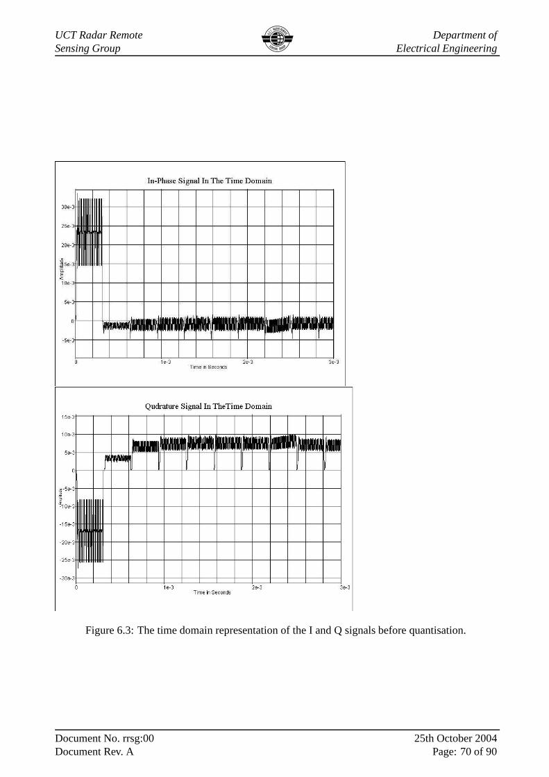
The output signals at the output of the I and Q channels are shown in figure 6.3. The time domain plots
shown here are at the input of the quantiser, before quantisation. The important aspect of this figure
is the average signal and noise voltage. The average noise voltage is important because it toggles the
Document No. rrsg:00Document Rev. A
25th October 2004Page: 68 of 90
UCT Radar RemoteSensing Group
Department ofElectrical Engineering
quantiser. As explained in subsection 5.3.3.2, a 14 bit quantiser with a 2 V voltage span has a stepsize
a = Vspan
214 = 122 × 10−3mV . To be able to do signal integration of the system, the thermal noise
must be greater thana/2 . The minimum average noise value between I and Q for this system was
1.879 × 10⁻¹mV which is greater thana/2 . This is done so that signal averaging in post processing
can be possible. The peak quantisation power for this systemis Pqnt,pk = 30 + 10log(a2/1250
) =
−16.05[dBm].
6.4 Range Binning
The first step in the computer processing of the stepped frequency signals is range binning, that is
organising the data in a range-frequency matrix. Each of the64 frequencies has 129 samples of it
taken both in the I and the Q channel. Each sample is a number. In each frequency an average value
of the sample numbers was taken for each I and Q. Since there are 64 frequency steps, it means 64
averages were taken forming 64 complex samplesI + jQ . This is shown below for onlyf0 , f1 and
f2 of the I channel.
1
fo f1 f2
channel
Io I I21
average average average
In Phase
129 258 387
Figure 6.4: This figure shows the number of samples that are taken for each frequency. An averageof the sample values is then taken which gives one I value. This figure only depicts three frequencies.
These complex samples form an array with 64 rows. The inversefast Fourier transform of these
complex was taken and the time plot is called the high range resolution profile. The number of
frequencies is in the x-axis of the plot and the y-axis represent the magnitude of the IFFT.
6.5 Range Profiling
The final step in the processing of the stepped frequency signal is range profiling. This was also done
using Matlab. The Matlab code shown in Appendix D, was used toplot the range profiles for this
comparison system. The formula of subsection 3.6.4 was usedto plot the range profile. This was
done in Matlab. The Matlab code is included in apppendix D. Figure 6.5 shows the range profiles of
Document No. rrsg:00Document Rev. A
25th October 2004Page: 69 of 90
UCT Radar RemoteSensing Group
Department ofElectrical Engineering
Figure 6.3: The time domain representation of the I and Q signals before quantisation.
Document No. rrsg:00Document Rev. A
25th October 2004Page: 70 of 90
UCT Radar RemoteSensing Group
Department ofElectrical Engineering
(a)
0 2 4 6 8 10 12
−0.04
−0.03
−0.02
−0.01
0
0.01
0.02
GeoMole BHR Model Pulse Range Profile
Range in metres
Pul
se A
mpl
itude
(b)
Figure 6.5: The Range Profiles of both the SFCW GPR and the GeoMole BHR Impulse radar systems.
Document No. rrsg:00Document Rev. A
25th October 2004Page: 71 of 90
UCT Radar RemoteSensing Group
Department ofElectrical Engineering
Transmitted Power,Pt Generated PowerP Transmitter Bandwidth Pulse Repetitive Period
26 dBm 48 dBm 100 MHz 550 ns
Transmitted VoltageVp Generated VoltageVp Pulse Repetition Frequency Pulse width
-65.29 V 1000 V 1.8018 MHz 8 ns
Table 6.1: GeoMole Transmitter Specifications
Gain Bandwidth Noise Figure Dynamic Range Penetration Depth Range Resolution
100 MHz 5 dB
Table 6.2: GeoMole Receiver Specifications
the SFCW and the impulse system. Because zero padding was notdone for the SFCW shown here,
the smooth peaking of the sinusoid with noise is now shown as noise. This was done so as to show the
effect of zero padding in signal processing. Plots are included in Appendix D that show a zero padded
signal and a signal that is not zero padded. With zero padding, the signal would be smooth. The peak
signal value at R = 15 m wasVp =0.055 and the average noise isVrms =0.015 for the SFCW. From
figure 6.5 (b) it was noted that the peak signal value at R = 5 m was 0.02 and the average noise is 0.
The peak signal to noise power for the SFCW is thereforePSNR = V 2p /Vrms =
6.6 GeoMole BoreHole Impulse Radar Specifications
The reader is referred to a dissertation by Guma et al [4] for the simulation, discussion and per-
formance testing of the GeoMole BHR impulse radar system referred to here. The transmitter and
receiver specification values for the GeoMole impulse radarare summarised in tables ?/ and ?/.
6.6.1 GeoMole Impulse Radar Transmitter
6.6.2 GeoMole Impulse Radar Receiver
6.7 SFCW GPR vs GeoMole BHR Impulse GPR
From table 6.2, the impulse radar has a receiver dynamic range of 74.8 dB and the SFCW GPR has
a dynamic range of 154 dB . The comparison between the SFCW andthe Impulse is shown in table
6.3. The stepped frequency radar transmits the smallest power but still proves to be the better system.
Document No. rrsg:00Document Rev. A
25th October 2004Page: 72 of 90
UCT Radar RemoteSensing Group
Department ofElectrical Engineering
SFCW GPR GeoMole BHR Impulse GPR
Pt 10 dBm 26 dBmL 10 dB 10 dB
SNR0 101.3 dB 5.09 dBDRl 154 dB 74.8 dBDRf 44.67 dB 47.47 dBRmax 15m [no stacking] 13.5 m [no stacking]
P1 12.7 dBm 13 dBm
P3 27 dBm 14.5 dBm
Table 6.3: The SFCW versus GeoMole BHR Impulse Radar.
6.8 Summary
The performance of a SFGPR system was found to be better than the impulse system as shown in
the table6.3. The SNR and linear DR of the SFCW was better thanthe impulse. The spurious free
dynamic range of the impulse is greater than that of the SFCW.The receiver of the SFCW was seen
to have a lower first order compression point, but a higher third-order point. The general SFCW
compared to the GeoMole BHR Impulse system was better.
Nonetheless, it was found that stacking of signals was impossible in SystemView for a SFCW since
memory ran out. This resulted into stacking not being performed for the SFCW system. It was
however found that stacking would possible in Matlab. This was not done because of time constraints.
A Matlab code for stacking 64 signals would have consumed much time and affect the completion of
the project. The stacking is thus mentioned here for future work.
Document No. rrsg:00Document Rev. A
25th October 2004Page: 73 of 90
UCT Radar RemoteSensing Group
Department ofElectrical Engineering
Chapter 7
Conclusion and Recommendations
Based on the findings of this report and the experience gainedduring the work, the following conclu-
sion can be drawn:
• A stepped frequency continuous wave ground penetrating radar was simulated using SystemView
and found to operate satisfactorily. Several limitations were found and recommendations on an
improved second simulation are given.
• A 1-100 MHz CW transmitter was simulated using the variable parameter method, and its
performance was tested. The transmitter performance was exceptional well. The spectrum
purity of the transmitter led to a good signal to noise ratio at the transmitter output. The phase
noise was found not degrading the performance of the transmitter. Even thou not all transmitted
signals were observed to have power level of 10 dBm, no frequency jitter was experienced in
the transmitter. The transmitter simulation was completedwith a transmit antenna simulated
with filter models and attenuators.
• The propagation medium simulation was kept simple. A bettermedium simulation was sug-
gested where the attenuation versus frequency relationship was used. Research had shown that
attenuation increases with frequency, this fact was used tosuggest an alternative to the simple
ground simulation. Furthermore, how this can be done in SystemView was described in great
detail.
• A heterodyne architecture receiver system was chosen over the homodyne because of its capa-
bilities. A 1-100 MHz CW receiver using a single IF system wassimulated, and its performance
tested. The dynamic range of this receiver was measured to bewhich is less than or greater than
. Improvements on the receiver simulation to increase the dynamic range are given in the rec-
ommendations.
Document No. rrsg:00Document Rev. A
25th October 2004Page: 74 of 90
UCT Radar RemoteSensing Group
Department ofElectrical Engineering
• The demodulation stage of the receiver was simulated and found to operate satisfactory. The
amount of noise signal at the demodulator output was found tobe important of signal averaging.
The mean noise value was used to toggle the quantiser, so thatwhen signal integration takes
place the signal would separates itself from noise.
• A Signal processing code was compiled in Matlab and used to obtain the high range resolution
of the radar. The code was found to operate unsatisfactory. The range profile obtained from the
code is shown in Appendix D. Improvements on the code are given in the recommendations.
The performance of the completed simulation was tested against a Geo Mole BHR impulse
radar system. Practically , the performance of the SFCW was found satisfactory. The linear
dynamic range of the SFCW was 79.2 dB above the impulse systemwhen the transmit power
of SFCW was 10 dBm. The transmit power of the GeoMole Impulse radar was calculated at
26 dBm and the losses in both systems were 10 dB. Also, both systems were simulated to have
antenna gains of 0 dB. The overall performance of the SFGPR radar compared to impulse radar
system is better.
Based on the findings of this report, the experienced gained through the work and the above conclu-
sions, recommendations on improvements on the system and future work are made. These recom-
mendations should be used to optimise the simulation into the next level.
7.1 Transmit Antenna Improvements
The transmit antenna simulation was merely done using filtermodels with a gain of 0 dB in the
passband for this simulation. It is recommended that , real antenna imperfections used in SFCW
GPR, be simulated and incorporated with this design. This will improve the signal to noise ratio at
the output of the transmitter even more.
7.2 Propagation Medium
The concept of developed in chapter 4, of the linear relationship between the attenuation and the
frequency should be investigated further. Ground models based on that concept will then be simulated
and incorporated in the simulation. This will drive the simulation more to the real SFCW GPR
simulator.
Document No. rrsg:00Document Rev. A
25th October 2004Page: 75 of 90
UCT Radar RemoteSensing Group
Department ofElectrical Engineering
7.3 Signal Processing
The time extent to which this project could be finished was underestimated. Therefore better signal
processing methods could not be covered. It is highly recommended to improve the signal processing
code used. Improvements on the code will result in huge improvements in the range profile plots.
Because also SystemView runs out of memory when stacking wasdone, methods that will eliminate
this problem can be of great significance.
Document No. rrsg:00Document Rev. A
25th October 2004Page: 76 of 90
UCT Radar RemoteSensing Group
Department ofElectrical Engineering
Bibliography
[1] Alan Langman,”Design of Hardware and Signal Processingfor a Stepped Frequency Continuous
Wave Ground Penetrating Radar”, PhD Thesis, University of Cape Town, March 2002
[2] D.A.Noon, “Stepped-Frequency Radar Design and Signal Processing Enhances Ground Pene-
trating Radar Performance”, PhD Thesis, Univeristy of Queensland,1996
[3] Richard Thomas Lord, “Aspects of Stepped-frequency Processing for Low-Frequency SAR sys-
tems”, PhD Thesis, University of Cape Town, 2000
[4] G.M. Kahimbaara, “Investigation and Simulation of an Impulse Ground Penetrating Radar Ap-
plication”, BSc. Thesis, University of Cape Town, 2004
[5] D.R. Wehner,“High Resolution Radar”, Norwood, MA : Artech House ,1995,
[6] M.I. Skolnik, “Introduction to Radar Systems”, McGraw-Hill, New York , USA, 1962
[7] M.I.Skolnik, “Radar Handbook”, McGraw-Hill, New York,NY, USA, 1990
[ 8] Marten Kabutz, “RF Hardware Design of a Stepped Frequency Continuous Wave Ground Pen-
etrating Radar”, MSc. Thesis, University of Cape Town, 1995
[9] James D. Taylor, “Ultra Wideband Radar Technology”, CRCPress, Boca Raton, FL, 2001
[10] J.C. Fowler, S.D. Hale, and R.T. Houck. Coal Mine HazardDetection Using Sythetic Pulse
Radar. RnMines OFR 79-81,ENSCO Inc., US Bereau of Mines Contract HO292925, January
1981.
[11] Gordon Farquharson, “Design and Implementing of a 200 -1600 MHz Stepped Frequency
Ground Penetrating Radar”, MSc. Thesis, University of CapeTown, 1999
[12] David M. Pozar, “ Microwave and RF Design, John Wiley & Sons, Inc. New York, 2001
[15] Michael K. Cope, ” Design, Simulation and Implementation of a digital Quadrature Demodula-
tor for a Stepped Frequency Radar”
[16] http:www//minicircuits.com/
[17] S.A. Hovanessian, “Radar System Design and Analysis”,Artech House, Norwood, MA, January
1984
Document No. rrsg:00Document Rev. A
25th October 2004Page: 78 of 90
UCT Radar RemoteSensing Group
Department ofElectrical Engineering
Appendix A
Dynamic Range
A.1 The Dynamic Range
Since thermal noise is generated by almost any lossy realistic component, the ideal linear component
does not exist in the sense that its output is always exactly proportional to its input excitation. Thus
all realistic components are non-linear at very low power levels due to noise effects. And all practi-
cal components become non-linear at high power levels.For instance, in amplifiers the gain tend to
decrease for large values of the output voltage, this effectis calledgain compressionor saturation.
Physically, this is usually due to the fact that the instantaneous output voltage of an amplifier is limited
by the power supply voltage used to bias the active device. Ineither case, these effects set a minimum
and maximum realistic power range ordynamic rangeover which a given component will operate as
desired.
To quantify the linear operating range of the amplifier, we define the1dB compression pointas the
power level for which the output power has decreased by 1dB from the ideal characteristic. This
power level is usually denoted byP1 , and can be stated in terms of either the input or the output
power. That is, either referred to the input or referred to the output. We then define intermodulation
distortion.
A.1.1 Intermodulation Distortion
Consider atwo toneinput voltage, consisting of two closely spaced frequencies,ω1 andω2 :
vi = V0(cosω1t + cosω2t)
The output voltage will consist of harmonics of the form
Document No. rrsg:00Document Rev. A
25th October 2004Page: 79 of 90
UCT Radar RemoteSensing Group
Department ofElectrical Engineering
ww
1w
22w−− w
12w − w
1 22w − w
2 1
2w2
2w1
3w 3w1 2
0
Figure A.1: Output spectrum of second and third order two-tone intermodulation products, assumingω1 < ω2 . This figure was taken from [12], but redrawn by the writer using Xfig.
mω1 + nω2
with m, n = 0,±1±2 ±3,.......These combinations of the two inputs frequencies are calledintermodu-
lation products, and theorderof a given product is defined as|m|+ |n|. All the second order products
are undesired in an amplifier, but in a mixer the sum or difference form the desired outputs. In either
case, ifω1 andω2 are close, all the second-order products will be far fromω1 or ω2, and can easily be
filtered (either passed or rejected) from the output of the component.
The cube term leads to six intermodulation products:3ω1, 3ω2, 2ω1 + ω2, 2ω2 + ω1, 2ω1 − ω2 and
2ω2 − ω1. The first four of these will be located far fromω1andω2 and will typically be outside the
passband of the component. But the two difference terms produce products located near the original
input signals as shown in figure A.1 , and so cannot be easily filtered from the passband of an amplifier.
Figure A.1 shows a typical spectrum of the second- and third-order two tone intermodulation products.
For an arbitrary input signal consisting of many frequencies of varying amplitude and phase, the
resulting in-band intermodulation products will cause distortion of the output signal. This effect is
calledthird order intermodulation distortion. Finally we define the third-order intercept point.
A.1.2 Third-Order Intercept Point
The output power of the first order, or linear product, is proportional to the input power and so the line
describing this response has a slope of unity before compression. The line describing the response
of the third-order products has a slope of three. The second-order products are outside the passband,
therefore do not affect the response. The linear and third -order responses will exhibit compression at
Document No. rrsg:00Document Rev. A
25th October 2004Page: 80 of 90
UCT Radar RemoteSensing Group
Department ofElectrical Engineering
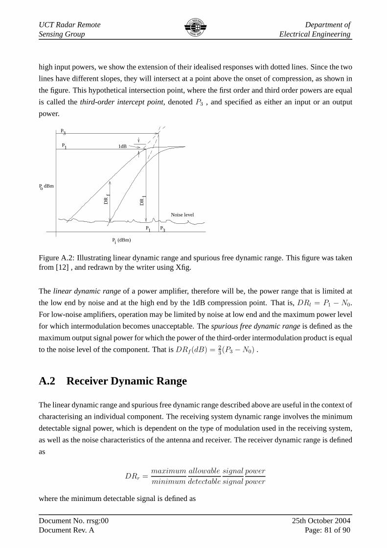
high input powers, we show the extension of their idealised responses with dotted lines. Since the two
lines have different slopes, they will intersect at a point above the onset of compression, as shown in
the figure. This hypothetical intersection point, where thefirst order and third order powers are equal
is called thethird-order intercept point, denotedP3 , and specified as either an input or an output
power.
P1
P3
Noise level
P (dBm)i
Po dBm
1dB
P P31
fD
R
DR
l
Figure A.2: Illustrating linear dynamic range and spuriousfree dynamic range. This figure was takenfrom [12] , and redrawn by the writer using Xfig.
The linear dynamic rangeof a power amplifier, therefore will be, the power range that is limited at
the low end by noise and at the high end by the 1dB compression point. That is,DRl = P1 − N0.
For low-noise amplifiers, operation may be limited by noise at low end and the maximum power level
for which intermodulation becomes unacceptable. Thespurious free dynamic rangeis defined as the
maximum output signal power for which the power of the third-order intermodulation product is equal
to the noise level of the component. That isDRf(dB) = 23(P3 − N0) .
A.2 Receiver Dynamic Range
The linear dynamic range and spurious free dynamic range described above are useful in the context of
characterising an individual component. The receiving system dynamic range involves the minimum
detectable signal power, which is dependent on the type of modulation used in the receiving system,
as well as the noise characteristics of the antenna and receiver. The receiver dynamic range is defined
as
DRr =maximum
minimum
allowable
detectable
signal
signal
power
power
where the minimum detectable signal is defined as
Document No. rrsg:00Document Rev. A
25th October 2004Page: 81 of 90
UCT Radar RemoteSensing Group
Department ofElectrical Engineering
Simin= kB(Ta + Te)(
S0
N0)min
and Ta is the antenna temperature,Te is the equivalent temperature of the receiving system, and
( S0
N0
)min is the minimum SNR required for that application. This appendix is an extract from Pozar et
al [12] , summarised by the writer.
Document No. rrsg:00Document Rev. A
25th October 2004Page: 82 of 90
UCT Radar RemoteSensing Group
Department ofElectrical Engineering
Appendix B
SystemView Figures
Because SystemView does not support copy of its token figuresinto Lyx. The SystemView token
figures were printed separately.
Figure B.1 is the simulation of the transmit antenna system,showing also the sinusoid that generates
the SFCW.
Figure B.2 is the figure showing demodulation.
Document No. rrsg:00Document Rev. A
25th October 2004Page: 83 of 90
UCT Radar RemoteSensing Group
Department ofElectrical Engineering
Figure B.1: SystemView Transmit Antenna
Document No. rrsg:00Document Rev. A
25th October 2004Page: 84 of 90
UCT Radar RemoteSensing Group
Department ofElectrical Engineering
Figure B.2: Receiver showing the down-conversion of the RF signal. The reference is mixed with thelocal oscillator and the output mixed with the received signal.
Document No. rrsg:00Document Rev. A
25th October 2004Page: 85 of 90
UCT Radar RemoteSensing Group
Department ofElectrical Engineering
Figure B.3: Demodulation in SystemView.
Document No. rrsg:00Document Rev. A
25th October 2004Page: 86 of 90
UCT Radar RemoteSensing Group
Department ofElectrical Engineering
Appendix C
Matlab Signal Processing
This is a Matlab code that was used to compute the average value per frequency for the I channel. The
code below was used in the comparison system of chapter 7, hence 64 frequencies. All these Matlab
code were compiled with the assistance of Guma Kahimbaara.
% this code computes the average sample
%value per frequency for the I channel
%there should be 64 average values since
%there are 64 frequencies per channel
I = Finalvalue_3pulses_Iout;
N =64; %Number of frequency steps
n =129; %Number of samples per frequency
Sv =0; %sum of all sample values per frequency
Sav = []; %average sample value for 129 samples
for i =1:N
for j = 1+((i-1)*129):129+((i-1)*129)
if j < 8193
Sv = Sv + I(j,2) %jth row second column
end
end
Sav(i)= Sv/129; %taking the average value of the sum
Sv = 0;
end
Sav
A similar code was used to obtain the 64 average values for theQ channel. The difference being the
data values that were used.
Document No. rrsg:00Document Rev. A
25th October 2004Page: 87 of 90
UCT Radar RemoteSensing Group
Department ofElectrical Engineering
Q = Finalvalue_3pulses_Iout;
N =64;
n =129;
Sv =0;
Sqav = [];
for i =1:N
for j = 1+((i-1)*129):129+((i-1)*129)
if j < 8193
Sv = Sv + I(j,2)
end
end
Sqav(i)= Sv/130;
Sv = 0;
end
Sqav
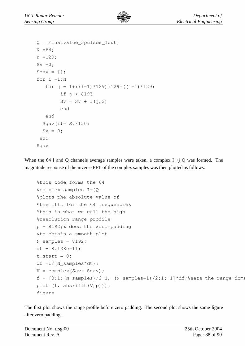
When the 64 I and Q channels average samples were taken, a complex I +j Q was formed. The
magnitude response of the inverse FFT of the complex sampleswas then plotted as follows:
%this code forms the 64
&complex samples I+jQ
%plots the absolute value of
%the ifft for the 64 frequencies
%this is what we call the high
%resolution range profile
p = 8192;% does the zero padding
&to obtain a smooth plot
N_samples = 8192;
dt = 8.138e-11;
t_start = 0;
df =1/(N_samples*dt);
V = complex(Sav, Sqav);
f = [0:1:(N_samples)/2-1,-(N_samples+1)/2:1:-1]*df;%sets the range domain
plot (f, abs(ifft(V,p)));
figure
The first plot shows the range profile before zero padding. Thesecond plot shows the same figure
after zero padding .
Document No. rrsg:00Document Rev. A
25th October 2004Page: 88 of 90
UCT Radar RemoteSensing Group
Department ofElectrical Engineering
(a)
(b)
Figure C.1: Range profiles for the comparison system showingbefore zero padding and after zeropadding.
Document No. rrsg:00Document Rev. A
25th October 2004Page: 89 of 90
UCT Radar RemoteSensing Group
Department ofElectrical Engineering
Zero padding was done onto the 64 frequencies in order to smooth the range profile plot. The plot had
sharp corners without zero padding. Thus it was very important that zero padding be implemented.
The concept of zero padding comes from the relationship between the number of frequency steps and
the range resolution. For a SFCW GPR withn = 64 and∆f = 1.5MHz , and bandwidth of 100
MHz transmitted for 20 ms. Each frequency is transmitted for312.5 microseconds. Without zero
padding or adding extra samples, the same time spacing wouldapply to the range profile in the time
domain. This will not lead to HRR, 312.5 IS > 10 ns.The IFFT of the 64 frequency steps leads to a
time domain profile with a two way time resolution of 10 nanoseconds.This is the ability to resolve
between two targets separated by a time t seconds.Nw zero padding adds extra samples in the time
domain, which makes high range resolution possible. With zero padding the samples are separated by
a very small time interval, and thus can resolve targets separated by small time space. That is, targets
separated by a small amount t will be resolved because there are more samples taken in the time plot.
As the number of frequency steps increases, the range resolution alos becomes better.