Design of an Automatic Defect Identification Method Based...

Research ArticleDesign of an Automatic Defect Identification Method BasedECPT for Pneumatic Pressure Equipment

Bo Zhang1 YuHua Cheng 1 Chun Yin 1 Xuegang Huang 2

Sara Dadras3 and Hadi Malek 3

1School of Automation Engineering University of Electronic Science and Technology of China Chengdu 611731 China2Hypervelocity Aerodynamics Institute China Aerodynamics Research amp Development Center Mianyang 621000 China3Electrical and Computer Engineering Department Utah State University Logan UT 84321 USA

Correspondence should be addressed to YuHua Cheng yhchenguestceducn

Received 4 July 2018 Revised 31 August 2018 Accepted 25 September 2018 Published 22 October 2018

Academic Editor Lingzhong Guo

Copyright copy 2018 Bo Zhang et alThis is an open access article distributed under theCreative Commons Attribution License whichpermits unrestricted use distribution and reproduction in any medium provided the original work is properly cited

In this paper in order to achieve automatic defect identification for pneumatic pressure equipment an improved feature extractionalgorithm eddy current pulsed thermography (ECPT) is presented The presented feature extraction algorithm contains fourelements data block selection variable step search relation value classification and between-class distance decision functionThe data block selection and variable step search are integrated to decrease the redundant computations in the automatic defectidentificationThe goal of the classification and between-class distance calculation is to select the typical features of thermographicsequenceThe main image information can be extracted by the method precisely and efficiently Experimental results are providedto demonstrate the capabilities and benefits (ie reducing the processing time) of the proposed algorithm in automatic defectidentification

1 Introduction

As one of the most significant energy storage and transmis-sion kind of equipment the pneumatic pressure equipmenthas been widely used in modern aerospace industries suchas manned spacecraft and ground wind tunnel testing inFigure 1 Moreover given its wide range of applications theequipment possesses a variety of specifications that make itflexibleThe flexibility of their specifications adds complexityto problem of inspecting and testing this important equip-ment to identify defects Researchers have studiedmethods tocharacterize pressure vessel properties in recent years J Leeet al proposed a method of estimating the design pressure ina prismatic storage vessel for liquefied natural gas [1] H Al-Gahtaniet et al studied the local pressure testing of sphericalvessels with nozzles [2] J Proczka et al reported guidelinesfor the efficient design and sizing of Small-Scale CompressedAir Energy Storage (SS-CAES) pressure vessels [3] P Blancstudied the residual burst pressure of composite cylindersafter mechanical impacts on their cylindrical part [4]

These studies however do not explore the impact of defectsrelated to the on-going use of pressure vesselsmade of diversematerials in a wide range of operating environments

The complicated usage environments and diversity ofmaterials cause the pneumatic pressure equipment to gener-ate fatigue cracks corrosion pits and other defects Thereforeit is important to detect the potential defects for the pressureequipment Nondestructive testing and evaluation (NDTampE)[5ndash10] are important to ensure the safety of manufacturingenvironments and equipment operation K Schabowicz et alpresented some nondestructive methods for the testing ofconcretemembers and fibre cement boards [11] Furthermorethe criteria for special specimen inspection are distinctso various detection methods are needed including surfacenondestructive testing appearance inspection and physic-ochemical test The surface nondestructive testing mainlyincludes magnetic particle testing and penetrant testing Dueto the advantages of surface nondestructive testing likehigh sensitivity and easy identification this method beenbroadly adopted However there are many problems that

HindawiComplexityVolume 2018 Article ID 5423924 16 pageshttpsdoiorg10115520185423924

2 Complexity

Figure 1 Pneumatic pressure equipment

need to be resolved in its practical application like highlabor intensity low efficiency pollution of the environmentpoor safety and so on In recent years ECPT has beendeveloping rapidly In addition to not damaging the bodythe method is fast is efficient and can solve the issues ofregular methods So in this paper the eddy current pulsedthermography is implemented in the detection of defects ofpneumatic pressure equipment Researchers also have madevaluable contributions in processing data [12ndash15] whichcan be applied in (NDTampE) P Zhu et al presented animproved feature extraction algorithm for automatic defectidentification based on eddy current pulsed thermography[16] H Yu utilized the normalized fuzzy weighting functionsto dispose the records of experiment [17]

Nevertheless the above-mentioned researches possesslow efficiency and limitations in processing data from low-alloy steel material Besides there are many methods suchas Independent Component Analysis (ICA) the processedfeature information will be distorted after restructuringbecause of data normalization lending to no visual effect indetection In recent years adaptive technique has gained a lotof interest to enhance the efficiency of processing data [18ndash21]To make the detection system be more useful for detectingthe defect it may own the ability of adapting property Anovel characteristic identification algorithm that uses thesimilarity of the typical transient thermal responses (119879119879119877119904)with the mixing vectors (the vectors of the pseudo-inversematrix of the demixing matrix) in ICA is proposed It solvesthe poor accuracy and low efficiency of the ICA efficientlyby using the choice of a known message The proposedalgorithm has four steps First the thermal imager collectsthe thermal image sequence of the pneumatic pressureequipment Second the 119879119879119877119904 are separated into parts usingthreshold values with a variable interval search The variableinterval search in an infrared image sequence can reducethe repetitive computation and hold the typical feature ofthe pneumatic pressure equipment Third the membershipmatrix and the clustering center are calculated to classify theacquired 119879119879119877119904 Moreover the rule of the largest distance oftwo class is used to identify the typical 119879119879119877119904 Fourth thetypical 119879119879119877119904 are transformed into a two-dimension matrix inlinear timeThemain features of the infrared image sequencein the pneumatic pressure equipment can be extracted by thetypical119879119879119877119904 Experimental results indicate the algorithm canselect the typical feature more precise than ones of the ICAFurthermore the processing time of the presented algorithmis shorter than ones of the ICATherefore the new algorithm

Figure 2 Pneumatic pressure equipment in China AerodynamicsResearch amp Development Center

can extract the main image information of the pneumaticpressure equipment accurately and efficiently in comparisonto the ICA

2 Background Pneumatic PressureEquipment and Nondestructive Testing

21 Pneumatic Pressure Equipment Themanufacture of highpressure vessels is complex involving the coordination ofsubject knowledge and professional technology in manyindustries including metallurgy corrosion and protectionmechanical processing safety protection chemical engineer-ing and testing The recent advances in technologies acrossvarious industries including nondestructive testing haveenabled considerable progress in pressure vessel manufactur-ing

(1) Varieties and specifications the types of materialcan be mainly divided into carbon steel low-alloy steeland a small amount of stainless steel Moreover the mainspecification of external diameter has dozens of kinds

(2) Complex usage environment pressure vessels andpipes often suffer from high pressure some special aerody-namic erosion and environmental corrosion in the open airwhich usually lead to cracks perforation fatigue damage andcorrosion of the equipment

(3) Devastating consequences of defects accidents notonly endanger the safety of personnel equipment and theplant but also lead to delay of test task failures and so on

22 Nondestructive Testing Surface nondestructive testing isthe key test method of pressure equipment such as pressurepiping and pressure vessels Surface nondestructive testingbasically includes magnetic particle testing and penetranttesting The method possesses numerous advantages such

Complexity 3

as high defect detection rate and high sensitivity But thereare also many problems including high labor intensity longoverhaul cycle low efficiency pollution of the environmentand poor safety So there exist a great many obstructorsfor development of detection skill In flammable explosiveenvironment because of the safety risks the traditional typesof surface nondestructive testing methods (magnetic particlepenetrant) cannot be implemented in the field

In recent years surface detection by eddy current hasbeen (developing) rapid In addition to not damaging thebody the method is fast and efficient and can achievelarge area rapid detection reducing manpower and materialresources The surface detection by eddy current is a methodthat utilizes thermal infrared image analysis

The temperature field distribution is based on a vortexphenomenon that can be measured using infrared detectionThe device is a thermal infrared imager with high speedand high resolution Moreover through the analysis ofthe infrared thermal image sequence we could detect thechanges of electromagnetic and thermal characteristics ofthe structure and material defects It can detect the surfaceand near surface by using the eddy current effect it alsocan detect deeper defects In the light of Joulersquos law theeddy current is turned into Joule heat in the testing piecegenerating high temperature and low temperature zonesTheinfrared thermal imager collects these temperature changesin the specimen The collected data are analyzed to computeanticorrelation results and detect the presence of defects

Eddy density can be indicated as 119869119890 = 120590 times (120597119860120597119905) inwhich 119860 expresses the magnetic vector bit and 120590 indicatesthe electrical conductivity ofmaterials In the depth directionthe eddy current density is 119869119890(119911) = 119869119890(0) sdot 119890minus119911radic120587120583120590119891 in which119911 is the depth 120583 is the permeability of testing material and119891 is the frequency of alternating current flowing through anexciting coil The depth of eddy density has an attenuation tothe 1119890 of the strength surface which is called as skin depth120575 = 1radic120587120583120590119891 According to Joulersquos law the heat power is119875119908 = (1120590)|119869119890|2 = (1120590)|120590119864|2 and E is electric field intensityThe Joule heat Q is transmitted inside the material and theheat propagation equation is 120588119862119901(120597119879120597119905) minus Δ(120590119879nabla119879) = 119876in which 120588 is material density 119862119901 is specific heat capacity ofmaterials 120590119879 is thermal conductivity of materials and 119879 istemperature of materials The crack depth is larger than eddycurrent skin depth in this specimen so

119869119890 = radic2120573119867radiccosh (2120573119909) minus cos (2120573119909)radiccosh (120573119887) + cos (120573119887)

(1)

in which 119887 is height H is magnetic field intensity and

120573 = radic120587119891120590120583 = 1120575 (2)

The thermal power in the unit volume of the two sidesof the crack is 119875119908 = 05(1120590) int 1198692119890119889119909 when the eddy skindepth is smaller than the plate thickness (120575 ≪ 119887) the thermalpower 119875119908 = 1205731198672(2120590) Recognizing the defects change theheat distribution in the parts or zones of a specimen the

principal component analysis enhances the zones where thethermal response and the eigenvector has similar trends Soin the enhancement of defects in a principal component theamplitude of other regionswill be inhibited and distributed ina very small range In this paper a new algorithm in view ofprincipal component selection is presented to automaticallyextract the principal components containing defects

3 Introduction of ProposedAlgorithm in ECPT

First of all some definitions are introduced in the Appendixto make the algorithm clear Then the proposed algorithm isexplicit as follows

Step 1 3D matrix 119863 saves the initial image sequence Everypixels value of thermal images is saved in the matrix 119863 Thethird-dimension of 119863 is the time axis t

Step 11 Search for 119863(119877119898119898 119862119898119898 119879119898119898) To find the length ofthe interval in the column coordinate this step sets (119870 =1 2 sdot sdot sdot 119896 sdot sdot sdot ) temperature thresholds 119879(119898) (119898 = 1 2 sdot sdot sdot 119870)from large to small moreover the row which includes thehighest temperature point 119863(119877119898119898 119862119898119898 119879119898119898) is divided into119870 + 1 parts

Step 12 Set temperature thresholds 119879 119862119871119896 for each partand the highest temperature point 119863119896(119877119898119898 119862119896 ) (119896 =1 2 sdot sdot sdot 119870) will be found in every part

Step 13 Set 119875 (119875 = 1 2 sdot sdot sdot 119901 sdot sdot sdot ) temperature thresholds119879(119899) (119899 = 1 2 sdot sdot sdot 119875) from large to small at the same timethe column which includes the highest temperature point119863(119877119898119898 119862119898119898 119879119898119898) is divided into 119875 + 1 parts After the rowis divided the temperature value of the column also shouldbe cut apart rationally in order to extract the characteristicsof the defect more accurately

Step 14 Set temperature thresholds 119879 119877119871119875 for each partand the highest temperature point 119863119901(119877119898119898 119862119901 ) (119901 =1 2 sdot sdot sdot 119875) will be found in every part The number of eachblock is regarded as 119897119890119899119901 (119901 = 1 2 sdot sdot sdot ) Moreover the samemethod as that of column is employed to find the row variableinterval 119877119871119901 The specific procedure of searching for intervalis in the following

(a) Set (119870 = 1 2 sdot sdot sdot 119896 sdot sdot sdot ) temperature thresholds todivide the 119879119879119877 into 119870 + 1 parts

(b) Set temperature thresholds 119879 119862119871119896 for each part(c) Search for the highest temperature point119863119896(119877119898119898 119862119896

)(d) Calculate the PCC of (119863119896(119877119898119898 119862119896 ) with 119863119896(119877119898119898

119888 ))(e) until their PCC is less than 119879 119862119871119896(f) The number of (119863119896(119877119898119898 119862119896 ) whose PCCs with

119863119896(119877119898119898 119888 )) are more than 119879 119862119871119896 is regarded as 119862119871119896(g) Set (119875 = 1 2 sdot sdot sdot 119901 sdot sdot sdot ) temperature thresholds to

divide the 119879119879119877 into 119875 + 1 parts(h)The same process as the searching for column interval

to find the row interval

4 Complexity

(i) The row interval is regarded as 119877119871119901

Step 15 What is more set the threshold DD initialize 119901 =1 119899 = 1 119911 = 1 and carry out the following procedures

(a) Set 119903 = 1 save the119863119901119896 (119903 119888 ) into the119883(119911 ) 119903 = 119903+119877119871119901

(b) If 119903 le 119897119890119899119901 Compute the PCC of 119863119901119896 (119903 119888 ) with

119883(119911 ) else go to step (d)(c) If 119875119862119862 lt 119863119863 119911 = 119911 + 1 119883(119911 ) = 119863119901

119896(119903 119888 ) 119903 =119903 + 119877119871119896 return step (b) else 119903 = 119903 + 119877119871119896 back to step (b)

(d) If 119903 lt 119872 119901 = 119901 + 1 119911 = 119911 + 1 back to step (a) else119888 = 119888 + 119862119871119896

(e) If 119888 lt 119897119890119899119896 back to step (a) else go to step (f)(f) If 119888 lt 119873 119896 = 119896 + 1 119888 = 1 back to step (a) else the

steps are finishedPneumatic pressure equipment includes high medium

and low pressure storage containers and inletoutlet gaspipelines as shown in Figure 2 The pneumatic pressureequipment stores and conveys compressed air The mainfeatures of these pressure vessels and the significance of theirdefect inspection are reflected in the following aspects

The specific calculation process is shown as Figure 3

Remark 1 For the interval 119862119871119896 the suitable method toseek out is searching for the length of region with largesttemperature variation What is more the 119879119879119877 with largestpeak value is always contained in the region with the largesttemperature variation As analysis of Step 1 the length ofregion with largest temperature variation can be found bythe coordinate value of 119879119862119871 For 119877119871119901 the homologoussetting rule is analogous to 119862119871119896 The proposed algorithmcan include the total typical temperature variations Andthe representative temperature variations express the featurein the corresponding image sequence characteristic pick-upalgorithm is put forward to handle data In the proposedalgorithm the appropriate interval values of column and row119862119868119896 (119896 = 1 2 sdot sdot sdot 119870)119877119868119901 (119901 = 1 2 sdot sdot sdot 119875) are set to reduce therepeated calculation Moreover the variable interval also cansave the significant features At the same time the proposedalgorithm possesses less redundant computation than ICA

Step 2 Divide 119883( 119911) into 119871 parts The specific calculationprocess is shown as Figure 4

(a) Set the cluster number L And at the same timeinitialize the cluster center 119898119900 moreover set the number ofiterations 119888 and set the weighting coefficient 119887 finally setterminating iterative threshold 120576

(b) Utilize formula to calculate membership function119906119895(119909119894) = 119889minus2(119887minus1)

119895119894 sum119871119904=1 119889minus2(119887minus1)

119904119894 in which 119894 = 1 2 sdot sdot sdot 119892119889119895119896 = 119883119896 minus 119898119895 119895 = 1 2 sdot sdot sdot 119871 119889119895119894 expresses the Euclideandistance between the 119894119905ℎ information weight value and the119895119905ℎ cluster center 119883119896 is the information weight value 119887is weighting coefficient 119906119895(119909119894) indicates the degree of theinformation weight value 119909119894 attached to the 119895119905ℎ part

(c) Update cluster center 119898119895 = sum119892119894=1[119906119895(119909119894)]119887119909119894

sum119892119894=1[119906119895(119909119894)]119887 in which119898119895 presents the 119895119905ℎ cluster center(d) Judge whether the absolute value of the objective

function difference is smaller than the threshold value If

119869119891(119888) minus 119869119891(119888 minus 1) ge 120576 and 119894 lt 119892 119894 = 119894 + 1 go back tostep (b) If 119894 gt 119892 and 119895 lt 119871 119895 = 119895 + 1 return to step (b) If119895 ge 119871 stop If 119869119891(119888) minus 119869119891(119888 minus 1) lt 120576 stop too

(e) The membership maximization rule is used to deblurall characteristic information weight and get the category ofeach information weight119872119896 = argmax(119906119895(119909119894))

Remark 2 Making use of the method of computing member-ship function and updating the clustering center in algorithmcan extract feature information accurately and effectivelyTaking advantage of the COV to classify data is called harddivision Hard division divides every object into a certaincategory strictly and each class is unrelated to each otherHowever the actual defect information objective exists inter-mediation in form and category Moreover there is no definiteboundary conditions to distinguish the class Thereforeclassifying the categories according to the membership andcluster centers of each class can bemore accurateThe featureinformation weights in each category represent the optimalweight of the feature information making the extractedfeatures more accurate and more reliable

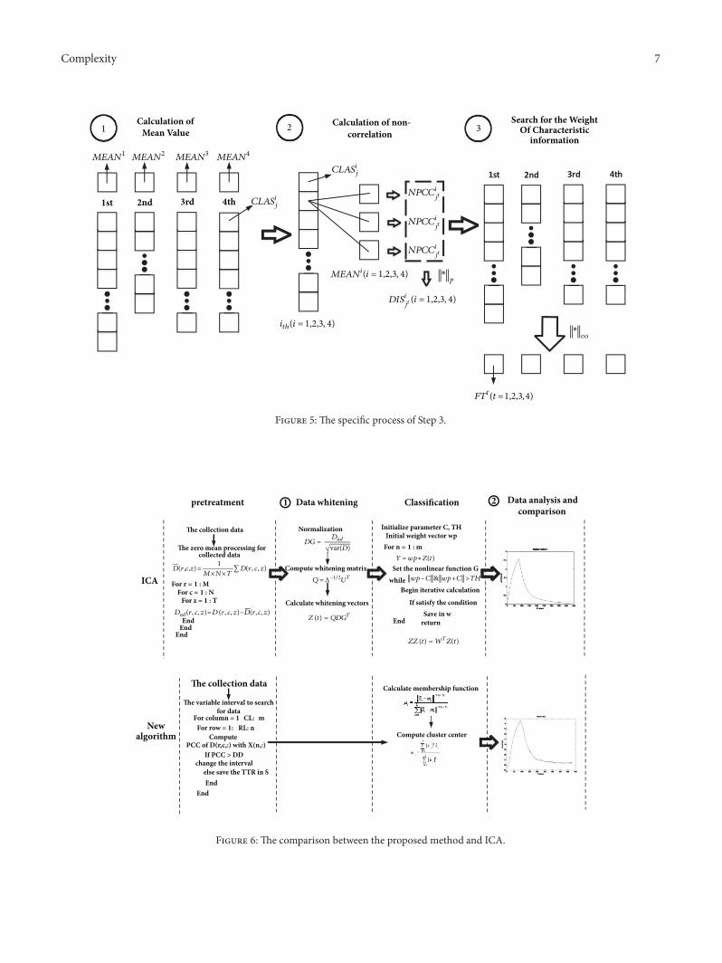
Step 3 The mean value of the 119894119905ℎ classification is 119872119864119860119873119894 =(1119877(119894))sum119895=12sdotsdotsdot 119877(119894) 119862119871119860119878119894119895 119894 = 1 2 sdot sdot sdot 119871 in which 119877(119894)presents the total number of 119879119879119877119904 in the 119894119905ℎ classification119873119875119862119862119894

119895119905 (119895 = 1 2 sdot sdot sdot 119877(119905)) is the noncorrelation value of119872119864119860119873119894 and 119862119871119860119878119905119895 119905 = 1 2 sdot sdot sdot 119871 and 119894 = 1 2 sdot sdot sdot 119905 minus 1 119905 +1 sdot sdot sdot 119871 (the 119895119905ℎ 119879119879119877 does not belong to the 119894119905ℎ classification)Let 119863119868119878119894119895119905 = 119873119875119862119862119894

119895119905119901 where 119863119868119878119894119895119905 expresses the distanceof two classes of 119879119879119877119904 119895 in the 119905119905ℎ classification with otherclasses In 119905119905ℎ (119905 = 1 2 sdot sdot sdot 119871) classification 119865119879119905 =119863119868119878119894119895119905infin in which 119865119879119905 is the final representation 119879119879119877 of 119905119905ℎclassification Save119865119879119905 (119905 = 1 2 sdot sdot sdot 119871) into119884 (ie119884( 119905) 119905 =1 2 sdot sdot sdot 119871 saves 119865119879119905 119905 = 1 2 sdot sdot sdot 119871) The specific calculationprocess is shown in Figure 5

Remark 3 The noncorrelation value of 119872119864119860119873119894 and 119862119871119860119878119905119895119905 = 1 2 sdot sdot sdot 119871 is expressed as 119873119875119862119862119894

119895119905 = 1 minus 119875119862119862(119872119864119860119873119894119862119871119860119878119905119895)

Remark 4 lowast119901 is P-norm lowastinfin is infinity-norm and lowast 119883 997888rarr 119877 satisfies the following

(1) positivity 119909 ge 0 and 119909 = 0 lArrrArr 119909 = 0(2) positivehomogeneity 119888119909 = |119888|119909(3) trigonometric inequality 119909+119910 le 119909 + 119910119909119901 = (|1199091|119901 + |1199091|119901 + sdot sdot sdot + |1199091|119901)1119901 and119909infin = max(|1199091| |1199092| sdot sdot sdot |119909119899|)

Remark 5 The purpose of the proposed algorithm in Step 1to Step 3 is to select the typical thermal responses Thesetypical responses have less intimately connection with eachother in ECPT The noncorrelation is larger and the thermalresponses are more representative Moreover the selectedaccurate data is classified by Steps 2 and 3 the cluster centerand membership function are carried out to classify thedefect feature The classification simplifies the data of imageprocessing and makes the postprocessing more precise

Complexity 5

RL

i = i minus M j = j + CLk

j + CLk gtN

i + RLP gtM

r = r + RLP

PCC gt DD

X(z)

z = z + 1X( z) = D(r c)

Get the final typical TTRs By means of the

way in above

NY

Y

Y

END

Transient thermal response

Search for typical TTRs in deferent column interval value

Block 1

Block 2

Block p

RL

RL

1

p

p

RL

RL

RL

RL

Through the different row

TTRs in row

Block 1 Block 2 Block k

1 2 22


Set temperature thresholds to divide

TTRs into many

Set r=1 c=1 z=1

interval value of correspondingblock Search for new typical

parts in row

Block 1

Block 2

Block p

N

N

Compute PCC of

CLCLCLCLCLCL k CLk1

with

2

2

2

D (r c)

1

Figure 3 The specific process of Step 1

Step 4 The 3119889 initial image sequence matrix 119863 will be trans-formed into 2119889 matrix 119880 The elements in one row of 119880 aretaken columnwise from 119863( 119901) 119901 = 1 2 sdot sdot sdot 119875 Calculate and solve this linear transformation 119878 = lowast 119880 in which expresses the pseudo-inverse matrix of 119884 and 119877 represents

the result of the proposed algorithm It includes the featuresof the initial image sequence processed by new algorithmMoreover continue to utilize the following way to achievethe extraction of defect feature 119874 = (1119873)sum(119909119910)isin119878 119891(119909 119910)in which 119874 expresses the mean of sum of the pixel values

6 Complexity

j lt L

i lt g

j = j + 1

i = i + 1

Jf(c) minus Jf(c minus 1) lt

djk =Xk minus mj

According to the maximumt

g

g

4

3

2

1

g

g

g

g

4L

3L

2L

1L

END

END

N

N

N

Y

Y

Y

Computer membership function

The weight of characteristic information

membership criterion the weight of

feature information is classified

Obtain the classified weightvalue of the characteristic

information

Computer distance

= g4g+ + +3g2g1g

Set c=100 L=4 i=1 j=1 =10minus5

j(xi) =dji

minus2(bminus1)

L

sums=1

dsiminus2(bminus1)

mj =

g

sumi=1

[j(xi)]bxi

g

sumi=1

[j(xi)]b

j(xi)

X( g)

X( g)

Xgtimest


f(x y) is the pixel values and 119873 is the number of pixelvalues Then we can obtain the uniform measurement of Sie max|119891(119909 119910) minus 119898|(119909119910)isin119878 lt 119881 in which 119881 is a thresholdFinally we can pick up the defect feature from the image

Remark 6 The final purpose of the proposed algorithm is toextract the defect feature and ignore redundant informationThemean value of selected region is obtained by the similaritycriterion of the method Moreover the calculation of theuniform measurement divides the region into defect featureand other areas

Remark 7 In order to highlight the efficiency and reason-ability of the proposed method the comparison of the ICAand the proposed algorithm is shown in Figure 6 In the

first part ldquoData whiteningrdquo the data in the ICA is dealtwith by normalization and then is computed to obtain thewhitening vectors according to the corresponding featurevectors and feature matrix These processes of calculationtake a lot of time to dispose data and reduce efficiencyof processing However the new algorithm does not havethese computational procedures to avoid the redundancycalculation Hence the amount of data in the proposedalgorithm after processing of pretreatment and whitening ismuch less than that in the ICA so in the postprocessingthe proposed algorithm avoids redundancy calculation andpossesses higher efficiency than the ICA 2) In the secondpart ldquoData analysis and comparisonrdquo compared with theextracted defect feature information graph the amplitudeof the graph extracted by the new algorithm contains the

Complexity 7

MEAN1 MEAN2 MEAN3 MEAN4

CLASij

CLASij

itℎ(i = 123 4)

NPCCij

NPCCij

NPCCij

(i = 123 4)MEANi lowastp

lowastinfin

(i = 123 4)DISij

(t =1234)FTt

Calculation of non- Search for the WeightOf Characteristic

information321 correlation

1st 2nd 3rd 4th

Calculation ofMean Value


D(rcz)= 1

MtimesNtimesTsumD(r c z)

Dad(r c z)=D(r c z)minusD(r cz)

DG =Dad

radicＰＬ(D)

Q=Λminus12UT

Z(t) = QDGT

ZZ(t) = WTZ(t)

wpminusCampwp+C

gtTHICA

1 2

algorithmNew

The collection data

Calculate whitening vectors

The variable interval to searchfor data

For column = 1 mCLnRLFor row = 1

Data whitening

Normalization

pretreatment Data analysis andcomparison

Classification

The zero mean processing for

EndEnd

End

EndEnd

collected data

The collection data

ComputePCC of D(rc) with X(n)

If PCC gt DDchange the interval

else save the TTR in S

Compute whitening matrix

For r = 1 MFor c = 1 N

For z = 1 T

Initialize parameter C TH

For n = 1 m

Set the nonlinear function G

Initial weight vector wp

whileBegin iterative calculation

If satisfy the conditionSave in w

Calculate membership function

End return

Compute cluster center

Y= wplowastZ(t)

Figure 6 The comparison between the proposed method and ICA

8 Complexity

PulseGenerator

Coil

IRCamera

Induction Heater

Excitation Signal

Specimen

Computer

Trigger Signal

Figure 7 The experimental schematic diagram

Figure 8 The damaged pneumatic pressure device

Defect

Defect

Figure 9 The specimen 1 and specimen 2

physical characteristics of the defect and the content iscloser to the defect feature information Thus the proposedalgorithm is more accurate and reasonable than the ICA

Remark 8 Step 1 realizes the segmentation of data block andthe calculation of column interval and row interval Step 2and Figure 3 show the process of the variable interval searchStep 3 is the correlation value classification Step 4 selectsthe 119871 typical 119879119879119877119904 based on the distance of two classes andextracts the typical features

4 Experimental Design

The setup of the experiment is shown in Figure 7 It includesfive functional parts induction heater coil PC timingtrigger and IR camera The induction heater produces highfrequency alternating current for coil excitation A rectangu-lar coil applies directional excitation to heat the sample Thetiming trigger controls the time for heating the sample TheIR camera records the thermal image sequence of the sampleThe analysis of experimental data is represented below

Figure 8 shows the damaged pneumatic pressure equip-ment All the test materials in this paper are provided bythe China Aerodynamics Research amp Development Centerwhich broadly supports research on aerodynamic equipmentIn view of the devices volume and degree of damagespecimen 1 and specimen 2 shown in Figure 9 are extractedfrom the pneumatic pressure equipment to analyze

Thedefects have beendetected using themethod of ECPTand the algorithm presented in Section 3 The two specimensare analyzed as follows For sample 1 the parameter index ofspecimen 1 is presented in Table 1

The process of Steps 3 and 4 is represented in Figure 10In Step 3 set p=1 b=1 c=100 120576 = 10minus5 There are 4613 35 and 2 119879119879119877119904 in the corresponding parts Throughthe algorithm of Step 3 in the 1119904119905 part compared withother 119879119879119877119904 the 2119899119889 possesses the maximum noncorrelation11986311986811987811989421 = 13124 The same as in the 2119899119889 part the 11(119905ℎ)possesses the maximum noncorrelation 119863119868119878119894112 = 13876 Inthe 3119903119889 part the 35119905ℎ possesses the maximum noncorrelation119863119868119878119894353 = 13097 In the 4119905ℎ the 1119904119905 possesses the maximumnoncorrelation 11986311986811987811989414 = 13951 1198791198791198771 1198791198791198772 1198791198791198773 and1198791198791198774 have been extracted by Steps 3 and 4 The extractionresults of proposed algorithm and the ICA result are shownin Figure 11 It is obvious that the features of the selected119879119879119877119904are similar to the ICs In Figure 12 the difference of 119879119879119877119904 isshown Comparing the proposed algorithm result with theresult of ICA in Figure 13 the trends of the red curves aresimilar to the blue curves respectively Moreover Figure 14illustrates the precise and accurate defect feature processedby the algorithm When comparing the proposed algorithmresult with the result of the ICA in Figure 15 the finalresult of the algorithm ignores more redundant informationthan the ICA result At the same time the defect featureextracted by the proposed algorithm is more precise andaccurate than the ICA result Consequently the algorithmhas selected the typical thermal responses and extractedmain features successfully The proposed method can notonly extract the main features like the ICA but also reducethe processed time substantially Its biggest advantage is theefficiency Figure 16 shows the processing time of the ICAand the proposed algorithm It is obvious that the proposedalgorithm needs less time to complete the feature extractionprocess

Complexity 9


j_th

Calculate non-correlation of

1st

2nd

3rd

4th

2

1

Calculate mean ofeach part

Calculation of noncorrelation

And search for thetypical CLASs

For the st part For the nd part

For the rd part For the th part

L_ st=

13

46

ndL_ =

24thL_ =

353

2

1

rdL_ =

MEAN1

MEAN2

MEAN3

MEAN4

j_th with MEANi

So in the stthe th

CLAS could be chosen

So in the rdthe th

CLAS could be chosenSo in the ththe th


So in the ndthe th


MEANi ==

1

R(i)sum

j 12middotmiddotmiddotR(i)

CLASij

CLASij

NPCCij

(i=123 4)

Figure 10 Steps 3 and 4 in proposed algorithm of sample 1

10 Complexity

New AlgorithmResult

Selected TTR ICA Result Mixing Vector

Mixing Vector 1

Mixing Vector 2

Mixing Vector 3

Mixing Vector 4

NO

1

2

3

4

50

100

150

200

250

300

350

400

450

50

100

150

200

250

300

350

400

450

50

100

150

200

250

300

350

400

450

50

100

150

200

250

300

350

400

450

TTR 1

TTR 2

TTR 3

TTR 4

600500400300200100

600500400300200100

600500400300200100

600500400300200100

50

100

150

200

250

300

350

400

450

600500400300200100

50

100

150

200

250

300

350

400

450

50

100

150

200

250

300

350

400

450

50

100

150

200

250

300

350

400

450

600500400300200100

600500400300200100

600500400300200100

1

08

06

04

02

0

Am

plitu

de

1

08

06

04

02

0

Am

plitu

de

1

08

06

04

02

0

Am

plitu

de

1

08

09

06

07

04

05

02

03

01

0

Am

plitu

de

1

08

09

06

07

04

05

02

03

01

0

Am

plitu

de

1

08

09

06

07

04

05

02

03

01

0

Am

plitu

de

1

08

09

06

07

04

05

02

03

01

0

Am

plitu

de

1

08

09

06

07

04

05

02

03

01

0

Am

plitu

de

Frames450400350300250200150100500

Frames450400350300250200150100500

Frames450400350300250200150100500

Frames450400350300250200150100500

Frames450400350300250200150100500

Frames450400350300250200150100500

Frames450400350300250200150100500

Frames450400350300250200150100500

Figure 11 The proposed algorithm and ICA result of sample 1

TTR i i=1234

TTR 1

TTR 2

TTR 3

TTR 4

0

02

04

06

08

Am

plitu

de

1

TTR 1TTR 2

TTR 3TTR 4

Frames450400350300250200150100500

Figure 12 The comparison of 1198791198791198771 1198791198791198772 1198791198791198773 and 1198791198791198774 of sample 1

Complexity 11

Mixing Vector 1 and TTR 1 Mixing Vector 2 and TTR 2 Mixing Vector 3 and TTR 3 Mixing Vector 4 and TTR 4


TTR 1Mixing Vector 1

Am

plitu

de

1

0

08

04

02

06

Am

plitu

de

1

0

08

04

02

06

Am

plitu

de

1

0

08

04

02

06

Am

plitu

de

1

0

08

04

02

06

TTR 1 Mixing Vector 1Frames

450400350300250200150100500

TTR 2

TTR 2

Mixing Vector 2

Mixing Vector 2

Frames450400350300250200150100500

TTR 3

TTR 3

Mixing Vector 3

Mixing Vector 3

Frames450400350300250200150100500

TTR 4

TTR 4

Mixing Vector 4

Mixing Vector 4

Frames450400350300250200150100500

Figure 13 The normalized mixing vector 1 mixing vector 2 mixing vector 3 mixing vector 4 and 1198791198791198771 1198791198791198772 1198791198791198773 and 1198791198791198774

Table 1 Parameter index of specimen 1

119878119886119898119901119897119890119879119894119898119890 119879119890119898119901119890119903119886119905119906119903119890119879ℎ119903119890119904ℎ119900119897119889119904 119879119867119877119864 119862119871 119877119864119865119877 11987117119904 119879(1) = 40 119879(2) = 80 098 1198771198641198651198771 = 098 1198771198641198651198772 = 096 1198771198641198651198773 = 094 2


119878119886119898119901119897119890119879119894119898119890 119879119890119898119901119890119903119886119905119906119903119890119879ℎ119903119890119904ℎ119900119897119889119904 119879119867119877119864 119862119871 119877119864119865119877 11987118119904 119879(1) = 29 119879(2) = 40 097 1198771198641198651198771 = 097 1198771198641198651198772 = 095 1198771198641198651198773 = 093 2

Defect

Figure 14 The defect feature of final result

For sample 2 the parameter index of specimen 2 ispresented in Table 2

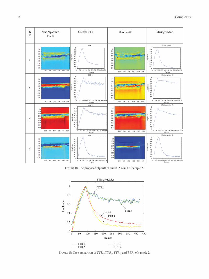
The process of Steps 3 and 4 is represented in Figure 17 InStep 3 set p=1 b=1 c=100 120576 = 10minus5 There are 30 30 24 and19 119879119879119877119904 in the corresponding parts Through the algorithmof Step 3 in the 1119904119905 part compared with other 119879119879119877119904 the 12119905ℎpossesses the maximum noncorrelation 119863119868119878119894121 = 16693The same as in the 2119899119889 part the 27119905ℎ possesses the maximumnoncorrelation 119863119868119878119894272 = 18238 In the 3119903119889 part the 6119905ℎpossesses the maximum noncorrelation 11986311986811987811989463 = 13921In the 4119905ℎ the 18119905ℎ possesses the maximum noncorrelation119863119868119878119894184 = 11842 1198791198791198771 1198791198791198772 1198791198791198773 and 1198791198791198774 havebeen extracted by Step 3 The extraction results of proposedalgorithm and the ICA result are shown in Figure 18 ThePearson correlation coefficients between mixing vectors 12 3 and 4 and 1198791198791198771 1198791198791198772 1198791198791198773 and 1198791198791198774 are 09786

09435 09678 and 09878 respectively It is obvious thatthe features of the selected 119879119879119877119904 are similar to the ICs InFigure 19 the difference of 119879119879119877119904 is shown Comparing theproposed algorithm result with the result of ICA in Figure 20the trends of the red curves are similar to the blue curvesrespectively Moreover Figure 21 illustrates the precise andaccurate defect feature processed by the algorithm Whencomparing the proposed algorithm result with the result ofthe ICA in Figure 22 the final result of the algorithm ignoresmore redundant information than the ICA result At the sametime the defect feature extracted by the proposed algorithm ismore precise and accurate than the ICA result Consequentlythe algorithm has selected the typical thermal responses andextracted main features successfully The proposed methodcan not only extract the main features like the ICA but alsoreduce the processed time substantially Its biggest advantageis the efficiency Figure 23 shows the processing time ofthe ICA and the proposed algorithm It is obvious that theproposed algorithm needs less time to complete the featureextraction process

5 Conclusion and Future Work

In this paper an accurate and more efficient algorithm inECPT is proposedThe validity and efficiency of the proposedmethod are demonstrated with experimental results Thephysical meaning of ECPT and the mathematical foundationof ICA are integrated in this proposed method The resultscontribute to advancing the use of ECPT to detect defects asfollows

(1) The primary features of the thermal image sequencescan be extracted by the proposed approach Meanwhile themain features can be utilized to detect defects

(2) Experimental results show that whitening preproce-dure is time-consuming The proposed algorithm has no data

12 Complexity

Specimen defect ICA Result Final Result

45040035030025020015010050

500 600400300200100

Figure 15 The specimen defect the ICA result and the final result

Table 3

119878119910119898119887119900119897 119873119900119905119886119905119894119900119899119904119863 3 dimensional matrix119877 the total number of rows in D119862 the all number of columns in D119885 the total number of the images at the t axis119863(119903 119888 ) the transient thermal response

119863(119877119898119898 119862119898119898 119879119898119898) the peak temperature point 119863(119877119898119898 119862119898119898 119879119898119898) =

max

119903 = 1 2 sdot sdot sdot119872119888 = 1 2 sdot sdot sdot 119873119905 = 1 2 sdot sdot sdot 119879

[119863(119903 119888 119905)]

119879119867119877119864 119862119871119896 the temperature thresholds in searching for the variable interval 119862119871119896


119897119890119899119896 the number of each block in searching for the variable interval 119862119871119896


(119863119901119896 (119903 119888 ) the transient thermal response in k part of row and p part of column

2 le 119871 le 119892 the final number of classifications in Step 2119875119862119862(119883119884) the computation of 119875119862119862(119883119884) = (1(119899 minus 1))sum119899

119894=1((119883119894 minus 119883)120590119883)((119884119894 minus 119884)120590119884)119862119871119860119878119894119895 the 119895119905ℎ 119879119879119877 of 119894119905ℎ class119895119905 the 119895119905ℎ 119879119879119877 in 119905119905ℎ classification

250

200

150

100

50

0

Tim

e (s)

The Processing Time

50376s

977s

Specimen 1ICA The new algorithm

Figure 16 The time comparison for specimen 1

whitening procedure So the proposed algorithm is moreeffective

(3) After processing of pretreatment and whiteningthe amount of data in the proposed algorithm is much

less than that of in ICA Hence in the postprocessingthe proposed algorithm avoids redundancy calculation andpossesses higher efficiency than the ICA So the proposedalgorithm is more accurate and reasonable than the ICA

Future work will pay more attention to how to enhancethe efficiency and accuracy of the novel algorithm In theexperiment some external interference will bring plentyof noise to influence the precision Moreover the changeof threshold values in the algorithm is also anticipated toimpact the efficiency of the detection Therefore it is worthresearching how to reduce the external interference and toadjust the threshold value

Appendix

Notations of the Proposed Algorithm

To make the algorithm explicit and clear the mathematicsdefinitions in the algorithm are shown in Table 3

Complexity 13


2

1

MEAN1

MEAN2

MEAN3

MEAN4


CLASij

194thL_ =

30ndL_ =2

L_ st=301

243rdL_ =

1st

2nd

3rd

4th

Calculation of non-correlation

And search for thetypical CLASs Calculate non-correlation of

j_th with MEANi

j_th


So in the stthe th

CLAS could be chosenSo in the ndthe th



So in the rdthe th



MEANi ==

1

R(i)sum


CLASij

NPCCij

(i=123 4)


14 Complexity

New AlgorithmResult


Mixing Vector 1

Mixing Vector 2

Mixing Vector 3

Mixing Vector 4

NO

1

2

3

4

50

100

150

200

250

300

350

400

450

50

100

150

200

250

300

350

400

450

50

100

150

200

250

300

350

400

450

50

100

150

200

250

300

350

400

450

TTR 1

TTR 2

TTR 3

TTR 4

600500400300200100

600500400300200100

600500400300200100

600500400300200100

50

100

150

200

250

300

350

400

450

600500400300200100

50

100

150

200

250

300

350

400

450

50

100

150

200

250

300

350

400

450

50100

150

200

250

300

350

400

450

600500400300200100

600500400300200100

600500400300200100

1

08

09

06

07

04

05

02

03

01

0

Am

plitu

de

1

0809

0607

0405

0203

010

Am

plitu

de

1

08

09

06

07

04

05

02

03

01

0

Am

plitu

de

1

0809

0607

0405

0203

010

Am

plitu

de

1

08

09

06

07

04

05

02

03

01

0

Am

plitu

de

1

0809

0607

0405

0203

010

Am

plitu

de

1

0809

0607

0405

0203

010

Am

plitu

de

1

0809

0607

0405

0203

010

Am

plitu

de

Frames450400350300250200150100500

Frames450400350300250200150100500

Frames450400350300250200150100500

Frames450400350300250200150100500

Frames450400350300250200150100500

Frames450400350300250200150100500

Frames450400350300250200150100500

Frames450400350300250200150100500


TTR i i=1234

0

02

04

06

08

Am

plitu

de

1

TTR 1TTR 2

Frames450400350300250200150100500

TTR 1

TTR 2

TTR 3

TTR 4

TTR 3TTR 4


Complexity 15



TTR 1Mixing Vector 1A

mpl

itude

1

0

08

04

02

06

Am

plitu

de

1

0

08

04

02

06

Am

plitu

de

1

0

08

04

02

06

Am

plitu

de

1

0

08

04

02

06


450400350300250200150100500


450400350300250200150100500


450400350300250200150100500


450400350300250200150100500

TTR 2 TTR 3

TTR 4Mixing Vector 2 Mixing Vector 3 Mixing Vector 4


Defect



45040035030025020015010050

500 600400300200100


ICA The new algorithmSpecimen 1

The Processing Time

7787s

634s

9080706050403020100

Tim

e (s)


16 Complexity

Data Availability

The data used to support the findings of this study areavailable from the corresponding author upon request

Conflicts of Interest

The authors declare that they have no conflicts of interest

Acknowledgments

This work was supported by National Basic Research Pro-gram of China (Grants nos 61873305 61671109 U183020751502338 and 61503064) 2018JY0410 Open Foundationof Hypervelocity Impact 20181102 and the FundamentalResearch Funds for the Central Universities

References

[1] J Lee Y Choi C Jo and D Chang ldquoDesign of a prismaticpressure vessel An engineering solution for non-stiffened-typevesselsrdquo Ocean Engineering vol 142 pp 639ndash649 2017

[2] H Al-Gahtani A Khathlan M Sunar and M Naffarsquoa ldquoLocalpressure testing of spherical vesselsrdquo International Journal ofPressure Vessels and Piping vol 114-115 pp 61ndash68 2014

[3] J J Proczka K Muralidharan D Villela J H Simmons and GFrantziskonis ldquoGuidelines for the pressure and efficient sizingof pressure vessels for compressed air energy storagerdquo EnergyConversion and Management vol 65 pp 597ndash605 2013

[4] P Blanc-Vannet ldquoBurst pressure reduction of various thermosetcomposite pressure vessels after impact on the cylindrical partrdquoComposite Structures vol 160 pp 706ndash711 2017

[5] X Maldague eory and Practice of Infrared Technology forNondestructive Testing John Wiley amp Sons 2001

[6] S Marinetti E Grinzato P G Bison et al ldquoStatistical analysisof IR thermographic sequences by PCArdquo Infrared Physics ampTechnology vol 46 no 1-2 pp 85ndash91 2004

[7] Y Cheng L Tian C Yin X Huang and L Bai ldquoA magneticdomain spots filtering method with self-adapting thresholdvalue selecting for crack detection based on theMOIrdquoNonlinearDynamics vol 86 no 2 pp 741ndash750 2016

[8] X Huang C Yin J Huang et al ldquoHypervelocity impactof TiB2-based composites as front bumpers for space shieldapplicationsrdquo Materials and Corrosion vol 97 pp 473ndash4822016

[9] X Xie D Yue H Zhang and Y Xue ldquoFault EstimationObserver Design for Discrete-Time Takagi-Sugeno Fuzzy Sys-tems Based on Homogenous Polynomially Parameter-Depend-ent LyapunovFunctionsrdquo IEEETransactions on Cybernetics vol47 no 9 pp 2504ndash2513 2017

[10] X Huang C Yin S Dadras Y Cheng and L Bai ldquoAdaptiverapid defect identification in ECPTbased onK-means and auto-matic segmentation algorithmrdquo Journal of Ambient Intelligenceand Humanized Computing pp 1ndash18 2017

[11] K Schabowicz and T Gorzelanczyk ldquoA nondestructive metho-dology for the testing of fibre cement boards by means ofa non-contact ultrasound scannerrdquo Construction and BuildingMaterials vol 102 pp 200ndash207 2016

[12] A Salazar L Vergar and R Llinares ldquoLearning material defectpatterns by separating mixtures of independent componentanalyzers from NDT sonic signalsrdquo Mechanical Systems andSignal Processing vol 24 no 6 pp 1870ndash1886 2010

[13] C-L Lim R Paramesran W Jassim Y-P Yu and K N NganldquoBlind image quality assessment for Gaussian blur images usingexact Zernikemoments and gradientmagnituderdquo Journal ofeFranklin Institute vol 353 no 17 pp 4715ndash4733 2016

[14] D Liu CWuQ Zhou and H-K Lam ldquoFuzzy guaranteed costoutput tracking control for fuzzy discrete-time systems withdifferent premise variablesrdquo Complexity vol 21 no 5 pp 265ndash276 2016

[15] P Liu and F Teng ldquoMultiple criteria decision making methodbased on normal interval-valued intuitionistic fuzzy general-ized aggregation operatorrdquo Complexity vol 21 no 5 pp 277ndash290 2016

[16] P Zhu C Yin Y Cheng et al ldquoAn improved feature extractionalgorithm for automatic defect identification based on eddycurrent pulsed thermographyrdquo Mechanical Systems amp SignalProcessing vol 113 pp 5ndash21 2018

[17] H Yu X Xie J Zhang D Ning and Y-W Jing ldquoRelaxed fuzzyobserver-based output feedback control synthesis of discrete-time nonlinear control systemsrdquo Complexity vol 21 no S1 pp593ndash601 2016

[18] J Cao K Zhang M Luo C Yin and X Lai ldquoExtreme learn-ingmachine and adaptive sparse representation for image class-ificationrdquo Neural Networks vol 81 pp 91ndash102 2016

[19] C Yin X Huang Y Chen S Dadras S-M Zhong and YCheng ldquoFractional-order exponential switching technique toenhance sliding mode controlrdquo Applied Mathematical Mod-elling Simulation and Computation for Engineering and Envi-ronmental Systems vol 44 pp 705ndash726 2017

[20] C Yin S Dadras X Huang J Mei H Malek and Y ChengldquoEnergy-saving control strategy for lighting system basedon multivariate extremum seeking with Newton algorithmrdquoEnergy Conversion andManagement vol 142 pp 504ndash522 2017

[21] Y Song Z Wang S Liu and G Wei ldquoN-step MPC with per-sistent bounded disturbances under stochastic communicationprotocolrdquo IEEE Transactions on Systems Man and CyberneticsSystems pp 1ndash11 2018

Hindawiwwwhindawicom Volume 2018

MathematicsJournal of


Mathematical Problems in Engineering

Applied MathematicsJournal of


Probability and StatisticsHindawiwwwhindawicom Volume 2018

Journal of


Mathematical PhysicsAdvances in

Complex AnalysisJournal of


OptimizationJournal of



Engineering Mathematics

International Journal of


Operations ResearchAdvances in

Journal of


Function SpacesAbstract and Applied AnalysisHindawiwwwhindawicom Volume 2018

International Journal of Mathematics and Mathematical Sciences


Hindawi Publishing Corporation httpwwwhindawicom Volume 2013Hindawiwwwhindawicom

The Scientific World Journal

Volume 2018

Hindawiwwwhindawicom Volume 2018Volume 2018

Numerical AnalysisNumerical AnalysisNumerical AnalysisNumerical AnalysisNumerical AnalysisNumerical AnalysisNumerical AnalysisNumerical AnalysisNumerical AnalysisNumerical AnalysisNumerical AnalysisNumerical AnalysisAdvances inAdvances in Discrete Dynamics in

Nature and SocietyHindawiwwwhindawicom Volume 2018

Hindawiwwwhindawicom

Dierential EquationsInternational Journal of

Volume 2018


Decision SciencesAdvances in


AnalysisInternational Journal of


Stochastic AnalysisInternational Journal of

Submit your manuscripts atwwwhindawicom

2 Complexity

Figure 1 Pneumatic pressure equipment

need to be resolved in its practical application like highlabor intensity low efficiency pollution of the environmentpoor safety and so on In recent years ECPT has beendeveloping rapidly In addition to not damaging the bodythe method is fast is efficient and can solve the issues ofregular methods So in this paper the eddy current pulsedthermography is implemented in the detection of defects ofpneumatic pressure equipment Researchers also have madevaluable contributions in processing data [12ndash15] whichcan be applied in (NDTampE) P Zhu et al presented animproved feature extraction algorithm for automatic defectidentification based on eddy current pulsed thermography[16] H Yu utilized the normalized fuzzy weighting functionsto dispose the records of experiment [17]

Nevertheless the above-mentioned researches possesslow efficiency and limitations in processing data from low-alloy steel material Besides there are many methods suchas Independent Component Analysis (ICA) the processedfeature information will be distorted after restructuringbecause of data normalization lending to no visual effect indetection In recent years adaptive technique has gained a lotof interest to enhance the efficiency of processing data [18ndash21]To make the detection system be more useful for detectingthe defect it may own the ability of adapting property Anovel characteristic identification algorithm that uses thesimilarity of the typical transient thermal responses (119879119879119877119904)with the mixing vectors (the vectors of the pseudo-inversematrix of the demixing matrix) in ICA is proposed It solvesthe poor accuracy and low efficiency of the ICA efficientlyby using the choice of a known message The proposedalgorithm has four steps First the thermal imager collectsthe thermal image sequence of the pneumatic pressureequipment Second the 119879119879119877119904 are separated into parts usingthreshold values with a variable interval search The variableinterval search in an infrared image sequence can reducethe repetitive computation and hold the typical feature ofthe pneumatic pressure equipment Third the membershipmatrix and the clustering center are calculated to classify theacquired 119879119879119877119904 Moreover the rule of the largest distance oftwo class is used to identify the typical 119879119879119877119904 Fourth thetypical 119879119879119877119904 are transformed into a two-dimension matrix inlinear timeThemain features of the infrared image sequencein the pneumatic pressure equipment can be extracted by thetypical119879119879119877119904 Experimental results indicate the algorithm canselect the typical feature more precise than ones of the ICAFurthermore the processing time of the presented algorithmis shorter than ones of the ICATherefore the new algorithm

Figure 2 Pneumatic pressure equipment in China AerodynamicsResearch amp Development Center

can extract the main image information of the pneumaticpressure equipment accurately and efficiently in comparisonto the ICA

2 Background Pneumatic PressureEquipment and Nondestructive Testing

21 Pneumatic Pressure Equipment Themanufacture of highpressure vessels is complex involving the coordination ofsubject knowledge and professional technology in manyindustries including metallurgy corrosion and protectionmechanical processing safety protection chemical engineer-ing and testing The recent advances in technologies acrossvarious industries including nondestructive testing haveenabled considerable progress in pressure vessel manufactur-ing

(1) Varieties and specifications the types of materialcan be mainly divided into carbon steel low-alloy steeland a small amount of stainless steel Moreover the mainspecification of external diameter has dozens of kinds

(2) Complex usage environment pressure vessels andpipes often suffer from high pressure some special aerody-namic erosion and environmental corrosion in the open airwhich usually lead to cracks perforation fatigue damage andcorrosion of the equipment

(3) Devastating consequences of defects accidents notonly endanger the safety of personnel equipment and theplant but also lead to delay of test task failures and so on

22 Nondestructive Testing Surface nondestructive testing isthe key test method of pressure equipment such as pressurepiping and pressure vessels Surface nondestructive testingbasically includes magnetic particle testing and penetranttesting The method possesses numerous advantages such

Complexity 3






(1)


120573 = radic120587119891120590120583 = 1120575 (2)

















4 Complexity
















119895119894 sum119871119904=1 119889minus2(119887minus1)












119895119905 = 1 minus 119875119862119862(119872119864119860119873119894119862119871119860119878119905119895)




Complexity 5

RL


j + CLk gtN

i + RLP gtM

r = r + RLP

PCC gt DD

X(z)

z = z + 1X( z) = D(r c)


way in above

NY

Y

Y

END



Block 1

Block 2

Block p

RL

RL

1

p

p

RL

RL

RL

RL


TTRs in row


1 2 22



TTRs into many

Set r=1 c=1 z=1


parts in row

Block 1

Block 2

Block p

N

N

Compute PCC of

CLCLCLCLCLCL k CLk1

with

2

2

2

D (r c)

1




6 Complexity

j lt L

i lt g

j = j + 1

i = i + 1


djk =Xk minus mj


g

g

4

3

2

1

g

g

g

g

4L

3L

2L

1L

END

END

N

N

N

Y

Y

Y






information

Computer distance

= g4g+ + +3g2g1g

Set c=100 L=4 i=1 j=1 =10minus5

j(xi) =dji

minus2(bminus1)

L

sums=1

dsiminus2(bminus1)

mj =

g

sumi=1

[j(xi)]bxi

g

sumi=1

[j(xi)]b

j(xi)

X( g)

X( g)

Xgtimest






Complexity 7


CLASij

CLASij

itℎ(i = 123 4)

NPCCij

NPCCij

NPCCij


lowastinfin

(i = 123 4)DISij

(t =1234)FTt



1st 2nd 3rd 4th



D(rcz)= 1



DG =Dad

radicＰＬ(D)

Q=Λminus12UT

Z(t) = QDGT

ZZ(t) = WTZ(t)

wpminusCampwp+C

gtTHICA

1 2

algorithmNew

The collection data




Data whitening

Normalization


Classification


EndEnd

End

EndEnd

collected data

The collection data






For z = 1 T


For n = 1 m






End return


Y= wplowastZ(t)


8 Complexity

PulseGenerator

Coil

IRCamera

Induction Heater

Excitation Signal

Specimen

Computer

Trigger Signal



Defect

Defect









Complexity 9


j_th


1st

2nd

3rd

4th

2

1






L_ st=

13

46

ndL_ =

24thL_ =

353

2

1

rdL_ =

MEAN1

MEAN2

MEAN3

MEAN4

j_th with MEANi

So in the stthe th


So in the rdthe th



So in the ndthe th


MEANi ==

1

R(i)sum


CLASij

CLASij

NPCCij

(i=123 4)


10 Complexity

New AlgorithmResult


Mixing Vector 1

Mixing Vector 2

Mixing Vector 3

Mixing Vector 4

NO

1

2

3

4

50

100

150

200

250

300

350

400

450

50

100

150

200

250

300

350

400

450

50

100

150

200

250

300

350

400

450

50

100

150

200

250

300

350

400

450

TTR 1

TTR 2

TTR 3

TTR 4

600500400300200100

600500400300200100

600500400300200100

600500400300200100

50

100

150

200

250

300

350

400

450

600500400300200100

50

100

150

200

250

300

350

400

450

50

100

150

200

250

300

350

400

450

50

100

150

200

250

300

350

400

450

600500400300200100

600500400300200100

600500400300200100

1

08

06

04

02

0

Am

plitu

de

1

08

06

04

02

0

Am

plitu

de

1

08

06

04

02

0

Am

plitu

de

1

08

09

06

07

04

05

02

03

01

0

Am

plitu

de

1

08

09

06

07

04

05

02

03

01

0

Am

plitu

de

1

08

09

06

07

04

05

02

03

01

0

Am

plitu

de

1

08

09

06

07

04

05

02

03

01

0

Am

plitu

de

1

08

09

06

07

04

05

02

03

01

0

Am

plitu

de

Frames450400350300250200150100500

Frames450400350300250200150100500

Frames450400350300250200150100500

Frames450400350300250200150100500

Frames450400350300250200150100500

Frames450400350300250200150100500

Frames450400350300250200150100500

Frames450400350300250200150100500


TTR i i=1234

TTR 1

TTR 2

TTR 3

TTR 4

0

02

04

06

08

Am

plitu

de

1

TTR 1TTR 2

TTR 3TTR 4

Frames450400350300250200150100500


Complexity 11




Am

plitu

de

1

0

08

04

02

06

Am

plitu

de

1

0

08

04

02

06

Am

plitu

de

1

0

08

04

02

06

Am

plitu

de

1

0

08

04

02

06


450400350300250200150100500

TTR 2

TTR 2

Mixing Vector 2

Mixing Vector 2

Frames450400350300250200150100500

TTR 3

TTR 3

Mixing Vector 3

Mixing Vector 3

Frames450400350300250200150100500

TTR 4

TTR 4

Mixing Vector 4

Mixing Vector 4

Frames450400350300250200150100500



119878119886119898119901119897119890119879119894119898119890 119879119890119898119901119890119903119886119905119906119903119890119879ℎ119903119890119904ℎ119900119897119889119904 119879119867119877119864 119862119871 119877119864119865119877 11987117119904 119879(1) = 40 119879(2) = 80 098 1198771198641198651198771 = 098 1198771198641198651198772 = 096 1198771198641198651198773 = 094 2


119878119886119898119901119897119890119879119894119898119890 119879119890119898119901119890119903119886119905119906119903119890119879ℎ119903119890119904ℎ119900119897119889119904 119879119867119877119864 119862119871 119877119864119865119877 11987118119904 119879(1) = 29 119879(2) = 40 097 1198771198641198651198771 = 097 1198771198641198651198772 = 095 1198771198641198651198773 = 093 2

Defect









12 Complexity


45040035030025020015010050

500 600400300200100


Table 3



max


[119863(119903 119888 119905)]








250

200

150

100

50

0

Tim

e (s)

The Processing Time

50376s

977s







Appendix



Complexity 13


2

1

MEAN1

MEAN2

MEAN3

MEAN4


CLASij

194thL_ =

30ndL_ =2

L_ st=301

243rdL_ =

1st

2nd

3rd

4th



j_th with MEANi

j_th


So in the stthe th




So in the rdthe th



MEANi ==

1

R(i)sum


CLASij

NPCCij

(i=123 4)


14 Complexity

New AlgorithmResult


Mixing Vector 1

Mixing Vector 2

Mixing Vector 3

Mixing Vector 4

NO

1

2

3

4

50

100

150

200

250

300

350

400

450

50

100

150

200

250

300

350

400

450

50

100

150

200

250

300

350

400

450

50

100

150

200

250

300

350

400

450

TTR 1

TTR 2

TTR 3

TTR 4

600500400300200100

600500400300200100

600500400300200100

600500400300200100

50

100

150

200

250

300

350

400

450

600500400300200100

50

100

150

200

250

300

350

400

450

50

100

150

200

250

300

350

400

450

50100

150

200

250

300

350

400

450

600500400300200100

600500400300200100

600500400300200100

1

08

09

06

07

04

05

02

03

01

0

Am

plitu

de

1

0809

0607

0405

0203

010

Am

plitu

de

1

08

09

06

07

04

05

02

03

01

0

Am

plitu

de

1

0809

0607

0405

0203

010

Am

plitu

de

1

08

09

06

07

04

05

02

03

01

0

Am

plitu

de

1

0809

0607

0405

0203

010

Am

plitu

de

1

0809

0607

0405

0203

010

Am

plitu

de

1

0809

0607

0405

0203

010

Am

plitu

de

Frames450400350300250200150100500

Frames450400350300250200150100500

Frames450400350300250200150100500

Frames450400350300250200150100500

Frames450400350300250200150100500

Frames450400350300250200150100500

Frames450400350300250200150100500

Frames450400350300250200150100500


TTR i i=1234

0

02

04

06

08

Am

plitu

de

1

TTR 1TTR 2

Frames450400350300250200150100500

TTR 1

TTR 2

TTR 3

TTR 4

TTR 3TTR 4


Complexity 15




mpl

itude

1

0

08

04

02

06

Am

plitu

de

1

0

08

04

02

06

Am

plitu

de

1

0

08

04

02

06

Am

plitu

de

1

0

08

04

02

06


450400350300250200150100500


450400350300250200150100500


450400350300250200150100500


450400350300250200150100500

TTR 2 TTR 3



Defect



45040035030025020015010050

500 600400300200100



The Processing Time

7787s

634s

9080706050403020100

Tim

e (s)


16 Complexity

Data Availability




Acknowledgments


References





























Journal of












Journal of







Volume 2018






Volume 2018








Complexity 3






(1)


120573 = radic120587119891120590120583 = 1120575 (2)

















4 Complexity
















119895119894 sum119871119904=1 119889minus2(119887minus1)












119895119905 = 1 minus 119875119862119862(119872119864119860119873119894119862119871119860119878119905119895)




Complexity 5

RL


j + CLk gtN

i + RLP gtM

r = r + RLP

PCC gt DD

X(z)

z = z + 1X( z) = D(r c)


way in above

NY

Y

Y

END



Block 1

Block 2

Block p

RL

RL

1

p

p

RL

RL

RL

RL


TTRs in row


1 2 22



TTRs into many

Set r=1 c=1 z=1


parts in row

Block 1

Block 2

Block p

N

N

Compute PCC of

CLCLCLCLCLCL k CLk1

with

2

2

2

D (r c)

1




6 Complexity

j lt L

i lt g

j = j + 1

i = i + 1


djk =Xk minus mj


g

g

4

3

2

1

g

g

g

g

4L

3L

2L

1L

END

END

N

N

N

Y

Y

Y






information

Computer distance

= g4g+ + +3g2g1g

Set c=100 L=4 i=1 j=1 =10minus5

j(xi) =dji

minus2(bminus1)

L

sums=1

dsiminus2(bminus1)

mj =

g

sumi=1

[j(xi)]bxi

g

sumi=1

[j(xi)]b

j(xi)

X( g)

X( g)

Xgtimest






Complexity 7


CLASij

CLASij

itℎ(i = 123 4)

NPCCij

NPCCij

NPCCij


lowastinfin

(i = 123 4)DISij

(t =1234)FTt



1st 2nd 3rd 4th



D(rcz)= 1



DG =Dad

radicＰＬ(D)

Q=Λminus12UT

Z(t) = QDGT

ZZ(t) = WTZ(t)

wpminusCampwp+C

gtTHICA

1 2

algorithmNew

The collection data




Data whitening

Normalization


Classification


EndEnd

End

EndEnd

collected data

The collection data






For z = 1 T


For n = 1 m






End return


Y= wplowastZ(t)


8 Complexity

PulseGenerator

Coil

IRCamera

Induction Heater

Excitation Signal

Specimen

Computer

Trigger Signal



Defect

Defect









Complexity 9


j_th


1st

2nd

3rd

4th

2

1






L_ st=

13

46

ndL_ =

24thL_ =

353

2

1

rdL_ =

MEAN1

MEAN2

MEAN3

MEAN4

j_th with MEANi

So in the stthe th


So in the rdthe th



So in the ndthe th


MEANi ==

1

R(i)sum


CLASij

CLASij

NPCCij

(i=123 4)


10 Complexity

New AlgorithmResult


Mixing Vector 1

Mixing Vector 2

Mixing Vector 3

Mixing Vector 4

NO

1

2

3

4

50

100

150

200

250

300

350

400

450

50

100

150

200

250

300

350

400

450

50

100

150

200

250

300

350

400

450

50

100

150

200

250

300

350

400

450

TTR 1

TTR 2

TTR 3

TTR 4

600500400300200100

600500400300200100

600500400300200100

600500400300200100

50

100

150

200

250

300

350

400

450

600500400300200100

50

100

150

200

250

300

350

400

450

50

100

150

200

250

300

350

400

450

50

100

150

200

250

300

350

400

450

600500400300200100

600500400300200100

600500400300200100

1

08

06

04

02

0

Am

plitu

de

1

08

06

04

02

0

Am

plitu

de

1

08

06

04

02

0

Am

plitu

de

1

08

09

06

07

04

05

02

03

01

0

Am

plitu

de

1

08

09

06

07

04

05

02

03

01

0

Am

plitu

de

1

08

09

06

07

04

05

02

03

01

0

Am

plitu

de

1

08

09

06

07

04

05

02

03

01

0

Am

plitu

de

1

08

09

06

07

04

05

02

03

01

0

Am

plitu

de

Frames450400350300250200150100500

Frames450400350300250200150100500

Frames450400350300250200150100500

Frames450400350300250200150100500

Frames450400350300250200150100500

Frames450400350300250200150100500

Frames450400350300250200150100500

Frames450400350300250200150100500


TTR i i=1234

TTR 1

TTR 2

TTR 3

TTR 4

0

02

04

06

08

Am

plitu

de

1

TTR 1TTR 2

TTR 3TTR 4

Frames450400350300250200150100500


Complexity 11




Am

plitu

de

1

0

08

04

02

06

Am

plitu

de

1

0

08

04

02

06

Am

plitu

de

1

0

08

04

02

06

Am

plitu

de

1

0

08

04

02

06


450400350300250200150100500

TTR 2

TTR 2

Mixing Vector 2

Mixing Vector 2

Frames450400350300250200150100500

TTR 3

TTR 3

Mixing Vector 3

Mixing Vector 3

Frames450400350300250200150100500

TTR 4

TTR 4

Mixing Vector 4

Mixing Vector 4

Frames450400350300250200150100500



119878119886119898119901119897119890119879119894119898119890 119879119890119898119901119890119903119886119905119906119903119890119879ℎ119903119890119904ℎ119900119897119889119904 119879119867119877119864 119862119871 119877119864119865119877 11987117119904 119879(1) = 40 119879(2) = 80 098 1198771198641198651198771 = 098 1198771198641198651198772 = 096 1198771198641198651198773 = 094 2


119878119886119898119901119897119890119879119894119898119890 119879119890119898119901119890119903119886119905119906119903119890119879ℎ119903119890119904ℎ119900119897119889119904 119879119867119877119864 119862119871 119877119864119865119877 11987118119904 119879(1) = 29 119879(2) = 40 097 1198771198641198651198771 = 097 1198771198641198651198772 = 095 1198771198641198651198773 = 093 2

Defect









12 Complexity


45040035030025020015010050

500 600400300200100


Table 3



max


[119863(119903 119888 119905)]








250

200

150

100

50

0

Tim

e (s)

The Processing Time

50376s

977s







Appendix



Complexity 13


2

1

MEAN1

MEAN2

MEAN3

MEAN4


CLASij

194thL_ =

30ndL_ =2

L_ st=301

243rdL_ =

1st

2nd

3rd

4th



j_th with MEANi

j_th


So in the stthe th




So in the rdthe th



MEANi ==

1

R(i)sum


CLASij

NPCCij

(i=123 4)


14 Complexity

New AlgorithmResult


Mixing Vector 1

Mixing Vector 2

Mixing Vector 3

Mixing Vector 4

NO

1

2

3

4

50

100

150

200

250

300

350

400

450

50

100

150

200

250

300

350

400

450

50

100

150

200

250

300

350

400

450

50

100

150

200

250

300

350

400

450

TTR 1

TTR 2

TTR 3

TTR 4

600500400300200100

600500400300200100

600500400300200100

600500400300200100

50

100

150

200

250

300

350

400

450

600500400300200100

50

100

150

200

250

300

350

400

450

50

100

150

200

250

300

350

400

450

50100

150

200

250

300

350

400

450

600500400300200100

600500400300200100

600500400300200100

1

08

09

06

07

04

05

02

03

01

0

Am

plitu

de

1

0809

0607

0405

0203

010

Am

plitu

de

1

08

09

06

07

04

05

02

03

01

0

Am

plitu

de

1

0809

0607

0405

0203

010

Am

plitu

de

1

08

09

06

07

04

05

02

03

01

0

Am

plitu

de

1

0809

0607

0405

0203

010

Am

plitu

de

1

0809

0607

0405

0203

010

Am

plitu

de

1

0809

0607

0405

0203

010

Am

plitu

de

Frames450400350300250200150100500

Frames450400350300250200150100500

Frames450400350300250200150100500

Frames450400350300250200150100500

Frames450400350300250200150100500

Frames450400350300250200150100500

Frames450400350300250200150100500

Frames450400350300250200150100500


TTR i i=1234

0

02

04

06

08

Am

plitu

de

1

TTR 1TTR 2

Frames450400350300250200150100500

TTR 1

TTR 2

TTR 3

TTR 4

TTR 3TTR 4


Complexity 15




mpl

itude

1

0

08

04

02

06

Am

plitu

de

1

0

08

04

02

06

Am

plitu

de

1

0

08

04

02

06

Am

plitu

de

1

0

08

04

02

06


450400350300250200150100500


450400350300250200150100500


450400350300250200150100500


450400350300250200150100500

TTR 2 TTR 3



Defect



45040035030025020015010050

500 600400300200100



The Processing Time

7787s

634s

9080706050403020100

Tim

e (s)


16 Complexity

Data Availability




Acknowledgments


References





























Journal of












Journal of







Volume 2018






Volume 2018








4 Complexity
















119895119894 sum119871119904=1 119889minus2(119887minus1)












119895119905 = 1 minus 119875119862119862(119872119864119860119873119894119862119871119860119878119905119895)




Complexity 5

RL


j + CLk gtN

i + RLP gtM

r = r + RLP

PCC gt DD

X(z)

z = z + 1X( z) = D(r c)


way in above

NY

Y

Y

END



Block 1

Block 2

Block p

RL

RL

1

p

p

RL

RL

RL

RL


TTRs in row


1 2 22



TTRs into many

Set r=1 c=1 z=1


parts in row

Block 1

Block 2

Block p

N

N

Compute PCC of

CLCLCLCLCLCL k CLk1

with

2

2

2

D (r c)

1




6 Complexity

j lt L

i lt g

j = j + 1

i = i + 1


djk =Xk minus mj


g

g

4

3

2

1

g

g

g

g

4L

3L

2L

1L

END

END

N

N

N

Y

Y

Y






information

Computer distance

= g4g+ + +3g2g1g

Set c=100 L=4 i=1 j=1 =10minus5

j(xi) =dji

minus2(bminus1)

L

sums=1

dsiminus2(bminus1)

mj =

g

sumi=1

[j(xi)]bxi

g

sumi=1

[j(xi)]b

j(xi)

X( g)

X( g)

Xgtimest






Complexity 7


CLASij

CLASij

itℎ(i = 123 4)

NPCCij

NPCCij

NPCCij


lowastinfin

(i = 123 4)DISij

(t =1234)FTt



1st 2nd 3rd 4th



D(rcz)= 1



DG =Dad

radicＰＬ(D)

Q=Λminus12UT

Z(t) = QDGT

ZZ(t) = WTZ(t)

wpminusCampwp+C

gtTHICA

1 2

algorithmNew

The collection data




Data whitening

Normalization


Classification


EndEnd

End

EndEnd

collected data

The collection data






For z = 1 T


For n = 1 m






End return


Y= wplowastZ(t)


8 Complexity

PulseGenerator

Coil

IRCamera

Induction Heater

Excitation Signal

Specimen

Computer

Trigger Signal



Defect

Defect









Complexity 9


j_th


1st

2nd

3rd

4th

2

1






L_ st=

13

46

ndL_ =

24thL_ =

353

2

1

rdL_ =

MEAN1

MEAN2

MEAN3

MEAN4

j_th with MEANi

So in the stthe th


So in the rdthe th



So in the ndthe th


MEANi ==

1

R(i)sum


CLASij

CLASij

NPCCij

(i=123 4)


10 Complexity

New AlgorithmResult


Mixing Vector 1

Mixing Vector 2

Mixing Vector 3

Mixing Vector 4

NO

1

2

3

4

50

100

150

200

250

300

350

400

450

50

100

150

200

250

300

350

400

450

50

100

150

200

250

300

350

400

450

50

100

150

200

250

300

350

400

450

TTR 1

TTR 2

TTR 3

TTR 4

600500400300200100

600500400300200100

600500400300200100

600500400300200100

50

100

150

200

250

300

350

400

450

600500400300200100

50

100

150

200

250

300

350

400

450

50

100

150

200

250

300

350

400

450

50

100

150

200

250

300

350

400

450

600500400300200100

600500400300200100

600500400300200100

1

08

06

04

02

0

Am

plitu

de

1

08

06

04

02

0

Am

plitu

de

1

08

06

04

02

0

Am

plitu

de

1

08

09

06

07

04

05

02

03

01

0

Am

plitu

de

1

08

09

06

07

04

05

02

03

01

0

Am

plitu

de

1

08

09

06

07

04

05

02

03

01

0

Am

plitu

de

1

08

09

06

07

04

05

02

03

01

0

Am

plitu

de

1

08

09

06

07

04

05

02

03

01

0

Am

plitu

de

Frames450400350300250200150100500

Frames450400350300250200150100500

Frames450400350300250200150100500

Frames450400350300250200150100500

Frames450400350300250200150100500

Frames450400350300250200150100500

Frames450400350300250200150100500

Frames450400350300250200150100500


TTR i i=1234

TTR 1

TTR 2

TTR 3

TTR 4

0

02

04

06

08

Am

plitu

de

1

TTR 1TTR 2

TTR 3TTR 4

Frames450400350300250200150100500


Complexity 11




Am

plitu

de

1

0

08

04

02

06

Am

plitu

de

1

0

08

04

02

06

Am

plitu

de

1

0

08

04

02

06

Am

plitu

de

1

0

08

04

02

06


450400350300250200150100500

TTR 2

TTR 2

Mixing Vector 2

Mixing Vector 2

Frames450400350300250200150100500

TTR 3

TTR 3

Mixing Vector 3

Mixing Vector 3

Frames450400350300250200150100500

TTR 4

TTR 4

Mixing Vector 4

Mixing Vector 4

Frames450400350300250200150100500



119878119886119898119901119897119890119879119894119898119890 119879119890119898119901119890119903119886119905119906119903119890119879ℎ119903119890119904ℎ119900119897119889119904 119879119867119877119864 119862119871 119877119864119865119877 11987117119904 119879(1) = 40 119879(2) = 80 098 1198771198641198651198771 = 098 1198771198641198651198772 = 096 1198771198641198651198773 = 094 2


119878119886119898119901119897119890119879119894119898119890 119879119890119898119901119890119903119886119905119906119903119890119879ℎ119903119890119904ℎ119900119897119889119904 119879119867119877119864 119862119871 119877119864119865119877 11987118119904 119879(1) = 29 119879(2) = 40 097 1198771198641198651198771 = 097 1198771198641198651198772 = 095 1198771198641198651198773 = 093 2

Defect









12 Complexity


45040035030025020015010050

500 600400300200100


Table 3



max


[119863(119903 119888 119905)]








250

200

150

100

50

0

Tim

e (s)

The Processing Time

50376s

977s







Appendix



Complexity 13


2

1

MEAN1

MEAN2

MEAN3

MEAN4


CLASij

194thL_ =

30ndL_ =2

L_ st=301

243rdL_ =

1st

2nd

3rd

4th



j_th with MEANi

j_th


So in the stthe th




So in the rdthe th



MEANi ==

1

R(i)sum


CLASij

NPCCij

(i=123 4)


14 Complexity

New AlgorithmResult


Mixing Vector 1

Mixing Vector 2

Mixing Vector 3

Mixing Vector 4

NO

1

2

3

4

50

100

150

200

250

300

350

400

450

50

100

150

200

250

300

350

400

450

50

100

150

200

250

300

350

400

450

50

100

150

200

250

300

350

400

450

TTR 1

TTR 2

TTR 3

TTR 4

600500400300200100

600500400300200100

600500400300200100

600500400300200100

50

100

150

200

250

300

350

400

450

600500400300200100

50

100

150

200

250

300

350

400

450

50

100

150

200

250

300

350

400

450

50100

150

200

250

300

350

400

450

600500400300200100

600500400300200100

600500400300200100

1

08

09

06

07

04

05

02

03

01

0

Am

plitu

de

1

0809

0607

0405

0203

010

Am

plitu

de

1

08

09

06

07

04

05

02

03

01

0

Am

plitu

de

1

0809

0607

0405

0203

010

Am

plitu

de

1

08

09

06

07

04

05

02

03

01

0

Am

plitu

de

1

0809

0607

0405

0203

010

Am

plitu

de

1

0809

0607

0405

0203

010

Am

plitu

de

1

0809

0607

0405

0203

010

Am

plitu

de

Frames450400350300250200150100500

Frames450400350300250200150100500

Frames450400350300250200150100500

Frames450400350300250200150100500

Frames450400350300250200150100500

Frames450400350300250200150100500

Frames450400350300250200150100500

Frames450400350300250200150100500


TTR i i=1234

0

02

04

06

08

Am

plitu

de

1

TTR 1TTR 2

Frames450400350300250200150100500

TTR 1

TTR 2

TTR 3

TTR 4

TTR 3TTR 4


Complexity 15




mpl

itude

1

0

08

04

02

06

Am

plitu

de

1

0

08

04

02

06

Am

plitu

de

1

0

08

04

02

06

Am

plitu

de

1

0

08

04

02

06


450400350300250200150100500


450400350300250200150100500


450400350300250200150100500


450400350300250200150100500

TTR 2 TTR 3



Defect



45040035030025020015010050

500 600400300200100



The Processing Time

7787s

634s

9080706050403020100

Tim

e (s)


16 Complexity

Data Availability




Acknowledgments


References





























Journal of












Journal of







Volume 2018






Volume 2018








Complexity 5

RL


j + CLk gtN

i + RLP gtM

r = r + RLP

PCC gt DD

X(z)

z = z + 1X( z) = D(r c)


way in above

NY

Y

Y

END



Block 1

Block 2

Block p

RL

RL

1

p

p

RL

RL

RL

RL


TTRs in row


1 2 22



TTRs into many

Set r=1 c=1 z=1


parts in row

Block 1

Block 2

Block p

N

N

Compute PCC of

CLCLCLCLCLCL k CLk1

with

2

2

2

D (r c)

1




6 Complexity

j lt L

i lt g

j = j + 1

i = i + 1


djk =Xk minus mj


g

g

4

3

2

1

g

g

g

g

4L

3L

2L

1L

END

END

N

N

N

Y

Y

Y






information

Computer distance

= g4g+ + +3g2g1g

Set c=100 L=4 i=1 j=1 =10minus5

j(xi) =dji

minus2(bminus1)

L

sums=1

dsiminus2(bminus1)

mj =

g

sumi=1

[j(xi)]bxi

g

sumi=1

[j(xi)]b

j(xi)

X( g)

X( g)

Xgtimest






Complexity 7


CLASij

CLASij

itℎ(i = 123 4)

NPCCij

NPCCij

NPCCij


lowastinfin

(i = 123 4)DISij

(t =1234)FTt



1st 2nd 3rd 4th



D(rcz)= 1



DG =Dad

radicＰＬ(D)

Q=Λminus12UT

Z(t) = QDGT

ZZ(t) = WTZ(t)

wpminusCampwp+C

gtTHICA

1 2

algorithmNew

The collection data




Data whitening

Normalization


Classification


EndEnd

End

EndEnd

collected data

The collection data






For z = 1 T


For n = 1 m






End return


Y= wplowastZ(t)


8 Complexity

PulseGenerator

Coil

IRCamera

Induction Heater

Excitation Signal

Specimen

Computer

Trigger Signal



Defect

Defect









Complexity 9


j_th


1st

2nd

3rd

4th

2

1






L_ st=

13

46

ndL_ =

24thL_ =

353

2

1

rdL_ =

MEAN1

MEAN2

MEAN3

MEAN4

j_th with MEANi

So in the stthe th


So in the rdthe th



So in the ndthe th


MEANi ==

1

R(i)sum


CLASij

CLASij

NPCCij

(i=123 4)


10 Complexity

New AlgorithmResult


Mixing Vector 1

Mixing Vector 2

Mixing Vector 3

Mixing Vector 4

NO

1

2

3

4

50

100

150

200

250

300

350

400

450

50

100

150

200

250

300

350

400

450

50

100

150

200

250

300

350

400

450

50

100

150

200

250

300

350

400

450

TTR 1

TTR 2

TTR 3

TTR 4

600500400300200100

600500400300200100

600500400300200100

600500400300200100

50

100

150

200

250

300

350

400

450

600500400300200100

50

100

150

200

250

300

350

400

450

50

100

150

200

250

300

350

400

450

50

100

150

200

250

300

350

400

450

600500400300200100

600500400300200100

600500400300200100

1

08

06

04

02

0

Am

plitu

de

1

08

06

04

02

0

Am

plitu

de

1

08

06

04

02

0

Am

plitu

de

1

08

09

06

07

04

05

02

03

01

0

Am

plitu

de

1

08

09

06

07

04

05

02

03

01

0

Am

plitu

de

1

08

09

06

07

04

05

02

03

01

0

Am

plitu

de

1

08

09

06

07

04

05

02

03

01

0

Am

plitu

de

1

08

09

06

07

04

05

02

03

01

0

Am

plitu

de

Frames450400350300250200150100500

Frames450400350300250200150100500

Frames450400350300250200150100500

Frames450400350300250200150100500

Frames450400350300250200150100500

Frames450400350300250200150100500

Frames450400350300250200150100500

Frames450400350300250200150100500


TTR i i=1234

TTR 1

TTR 2

TTR 3

TTR 4

0

02

04

06

08

Am

plitu

de

1

TTR 1TTR 2

TTR 3TTR 4

Frames450400350300250200150100500


Complexity 11




Am

plitu

de

1

0

08

04

02

06

Am

plitu

de

1

0

08

04

02

06

Am

plitu

de

1

0

08

04

02

06

Am

plitu

de

1

0

08

04

02

06


450400350300250200150100500

TTR 2

TTR 2

Mixing Vector 2

Mixing Vector 2

Frames450400350300250200150100500

TTR 3

TTR 3

Mixing Vector 3

Mixing Vector 3

Frames450400350300250200150100500

TTR 4

TTR 4

Mixing Vector 4

Mixing Vector 4

Frames450400350300250200150100500



119878119886119898119901119897119890119879119894119898119890 119879119890119898119901119890119903119886119905119906119903119890119879ℎ119903119890119904ℎ119900119897119889119904 119879119867119877119864 119862119871 119877119864119865119877 11987117119904 119879(1) = 40 119879(2) = 80 098 1198771198641198651198771 = 098 1198771198641198651198772 = 096 1198771198641198651198773 = 094 2


119878119886119898119901119897119890119879119894119898119890 119879119890119898119901119890119903119886119905119906119903119890119879ℎ119903119890119904ℎ119900119897119889119904 119879119867119877119864 119862119871 119877119864119865119877 11987118119904 119879(1) = 29 119879(2) = 40 097 1198771198641198651198771 = 097 1198771198641198651198772 = 095 1198771198641198651198773 = 093 2

Defect









12 Complexity


45040035030025020015010050

500 600400300200100


Table 3



max


[119863(119903 119888 119905)]








250

200

150

100

50

0

Tim

e (s)

The Processing Time

50376s

977s







Appendix



Complexity 13


2

1

MEAN1

MEAN2

MEAN3

MEAN4


CLASij

194thL_ =

30ndL_ =2

L_ st=301

243rdL_ =

1st

2nd

3rd

4th



j_th with MEANi

j_th


So in the stthe th




So in the rdthe th



MEANi ==

1

R(i)sum


CLASij

NPCCij

(i=123 4)


14 Complexity

New AlgorithmResult


Mixing Vector 1

Mixing Vector 2

Mixing Vector 3

Mixing Vector 4

NO

1

2

3

4

50

100

150

200

250

300

350

400

450

50

100

150

200

250

300

350

400

450

50

100

150

200

250

300

350

400

450

50

100

150

200

250

300

350

400

450

TTR 1

TTR 2

TTR 3

TTR 4

600500400300200100

600500400300200100

600500400300200100

600500400300200100

50

100

150

200

250

300

350

400

450

600500400300200100

50

100

150

200

250

300

350

400

450

50

100

150

200

250

300

350

400

450

50100

150

200

250

300

350

400

450

600500400300200100

600500400300200100

600500400300200100

1

08

09

06

07

04

05

02

03

01

0

Am

plitu

de

1

0809

0607

0405

0203

010

Am

plitu

de

1

08

09

06

07

04

05

02

03

01

0

Am

plitu

de

1

0809

0607

0405

0203

010

Am

plitu

de

1

08

09

06

07

04

05

02

03

01

0

Am

plitu

de

1

0809

0607

0405

0203

010

Am

plitu

de

1

0809

0607

0405

0203

010

Am

plitu

de

1

0809

0607

0405

0203

010

Am

plitu

de

Frames450400350300250200150100500

Frames450400350300250200150100500

Frames450400350300250200150100500

Frames450400350300250200150100500

Frames450400350300250200150100500

Frames450400350300250200150100500

Frames450400350300250200150100500

Frames450400350300250200150100500


TTR i i=1234

0

02

04

06

08

Am

plitu

de

1

TTR 1TTR 2

Frames450400350300250200150100500

TTR 1

TTR 2

TTR 3

TTR 4

TTR 3TTR 4


Complexity 15




mpl

itude

1

0

08

04

02

06

Am

plitu

de

1

0

08

04

02

06

Am

plitu

de

1

0

08

04

02

06

Am

plitu

de

1

0

08

04

02

06


450400350300250200150100500


450400350300250200150100500


450400350300250200150100500


450400350300250200150100500

TTR 2 TTR 3



Defect



45040035030025020015010050

500 600400300200100



The Processing Time

7787s

634s

9080706050403020100

Tim

e (s)


16 Complexity

Data Availability




Acknowledgments


References





























Journal of












Journal of







Volume 2018






Volume 2018








6 Complexity

j lt L

i lt g

j = j + 1

i = i + 1


djk =Xk minus mj


g

g

4

3

2

1

g

g

g

g

4L

3L

2L

1L

END

END

N

N

N

Y

Y

Y






information

Computer distance

= g4g+ + +3g2g1g

Set c=100 L=4 i=1 j=1 =10minus5

j(xi) =dji

minus2(bminus1)

L

sums=1

dsiminus2(bminus1)

mj =

g

sumi=1

[j(xi)]bxi

g

sumi=1

[j(xi)]b

j(xi)

X( g)

X( g)

Xgtimest






Complexity 7


CLASij

CLASij

itℎ(i = 123 4)

NPCCij

NPCCij

NPCCij


lowastinfin

(i = 123 4)DISij

(t =1234)FTt



1st 2nd 3rd 4th



D(rcz)= 1



DG =Dad

radicＰＬ(D)

Q=Λminus12UT

Z(t) = QDGT

ZZ(t) = WTZ(t)

wpminusCampwp+C

gtTHICA

1 2

algorithmNew

The collection data




Data whitening

Normalization


Classification


EndEnd

End

EndEnd

collected data

The collection data






For z = 1 T


For n = 1 m






End return


Y= wplowastZ(t)


8 Complexity

PulseGenerator

Coil

IRCamera

Induction Heater

Excitation Signal

Specimen

Computer

Trigger Signal



Defect

Defect









Complexity 9


j_th


1st

2nd

3rd

4th

2

1






L_ st=

13

46

ndL_ =

24thL_ =

353

2

1

rdL_ =

MEAN1

MEAN2

MEAN3

MEAN4

j_th with MEANi

So in the stthe th


So in the rdthe th



So in the ndthe th


MEANi ==

1

R(i)sum


CLASij

CLASij

NPCCij

(i=123 4)


10 Complexity

New AlgorithmResult


Mixing Vector 1

Mixing Vector 2

Mixing Vector 3

Mixing Vector 4

NO

1

2

3

4

50

100

150

200

250

300

350

400

450

50

100

150

200

250

300

350

400

450

50

100

150

200

250

300

350

400

450

50

100

150

200

250

300

350

400

450

TTR 1

TTR 2

TTR 3

TTR 4

600500400300200100

600500400300200100

600500400300200100

600500400300200100

50

100

150

200

250

300

350

400

450

600500400300200100

50

100

150

200

250

300

350

400

450

50

100

150

200

250

300

350

400

450

50

100

150

200

250

300

350

400

450

600500400300200100

600500400300200100

600500400300200100

1

08

06

04

02

0

Am

plitu

de

1

08

06

04

02

0

Am

plitu

de

1

08

06

04

02

0

Am

plitu

de

1

08

09

06

07

04

05

02

03

01

0

Am

plitu

de

1

08

09

06

07

04

05

02

03

01

0

Am

plitu

de

1

08

09

06

07

04

05

02

03

01

0

Am

plitu

de

1

08

09

06

07

04

05

02

03

01

0

Am

plitu

de

1

08

09

06

07

04

05

02

03

01

0

Am

plitu

de

Frames450400350300250200150100500

Frames450400350300250200150100500

Frames450400350300250200150100500

Frames450400350300250200150100500

Frames450400350300250200150100500

Frames450400350300250200150100500

Frames450400350300250200150100500

Frames450400350300250200150100500


TTR i i=1234

TTR 1

TTR 2

TTR 3

TTR 4

0

02

04

06

08

Am

plitu

de

1

TTR 1TTR 2

TTR 3TTR 4

Frames450400350300250200150100500


Complexity 11




Am

plitu

de

1

0

08

04

02

06

Am

plitu

de

1

0

08

04

02

06

Am

plitu

de

1

0

08

04

02

06

Am

plitu

de

1

0

08

04

02

06


450400350300250200150100500

TTR 2

TTR 2

Mixing Vector 2

Mixing Vector 2

Frames450400350300250200150100500

TTR 3

TTR 3

Mixing Vector 3

Mixing Vector 3

Frames450400350300250200150100500

TTR 4

TTR 4

Mixing Vector 4

Mixing Vector 4

Frames450400350300250200150100500



119878119886119898119901119897119890119879119894119898119890 119879119890119898119901119890119903119886119905119906119903119890119879ℎ119903119890119904ℎ119900119897119889119904 119879119867119877119864 119862119871 119877119864119865119877 11987117119904 119879(1) = 40 119879(2) = 80 098 1198771198641198651198771 = 098 1198771198641198651198772 = 096 1198771198641198651198773 = 094 2


119878119886119898119901119897119890119879119894119898119890 119879119890119898119901119890119903119886119905119906119903119890119879ℎ119903119890119904ℎ119900119897119889119904 119879119867119877119864 119862119871 119877119864119865119877 11987118119904 119879(1) = 29 119879(2) = 40 097 1198771198641198651198771 = 097 1198771198641198651198772 = 095 1198771198641198651198773 = 093 2

Defect









12 Complexity


45040035030025020015010050

500 600400300200100


Table 3



max


[119863(119903 119888 119905)]








250

200

150

100

50

0

Tim

e (s)

The Processing Time

50376s

977s







Appendix



Complexity 13


2

1

MEAN1

MEAN2

MEAN3

MEAN4


CLASij

194thL_ =

30ndL_ =2

L_ st=301

243rdL_ =

1st

2nd

3rd

4th



j_th with MEANi

j_th


So in the stthe th




So in the rdthe th



MEANi ==

1

R(i)sum


CLASij

NPCCij

(i=123 4)


14 Complexity

New AlgorithmResult


Mixing Vector 1

Mixing Vector 2

Mixing Vector 3

Mixing Vector 4

NO

1

2

3

4

50

100

150

200

250

300

350

400

450

50

100

150

200

250

300

350

400

450

50

100

150

200

250

300

350

400

450

50

100

150

200

250

300

350

400

450

TTR 1

TTR 2

TTR 3

TTR 4

600500400300200100

600500400300200100

600500400300200100

600500400300200100

50

100

150

200

250

300

350

400

450

600500400300200100

50

100

150

200

250

300

350

400

450

50

100

150

200

250

300

350

400

450

50100

150

200

250

300

350

400

450

600500400300200100

600500400300200100

600500400300200100

1

08

09

06

07

04

05

02

03

01

0

Am

plitu

de

1

0809

0607

0405

0203

010

Am

plitu

de

1

08

09

06

07

04

05

02

03

01

0

Am

plitu

de

1

0809

0607

0405

0203

010

Am

plitu

de

1

08

09

06

07

04

05

02

03

01

0

Am

plitu

de

1

0809

0607

0405

0203

010

Am

plitu

de

1

0809

0607

0405

0203

010

Am

plitu

de

1

0809

0607

0405

0203

010

Am

plitu

de

Frames450400350300250200150100500

Frames450400350300250200150100500

Frames450400350300250200150100500

Frames450400350300250200150100500

Frames450400350300250200150100500

Frames450400350300250200150100500

Frames450400350300250200150100500

Frames450400350300250200150100500


TTR i i=1234

0

02

04

06

08

Am

plitu

de

1

TTR 1TTR 2

Frames450400350300250200150100500

TTR 1

TTR 2

TTR 3

TTR 4

TTR 3TTR 4


Complexity 15




mpl

itude

1

0

08

04

02

06

Am

plitu

de

1

0

08

04

02

06

Am

plitu

de

1

0

08

04

02

06

Am

plitu

de

1

0

08

04

02

06


450400350300250200150100500


450400350300250200150100500


450400350300250200150100500


450400350300250200150100500

TTR 2 TTR 3



Defect



45040035030025020015010050

500 600400300200100



The Processing Time

7787s

634s

9080706050403020100

Tim

e (s)


16 Complexity

Data Availability




Acknowledgments


References





























Journal of












Journal of







Volume 2018






Volume 2018








Complexity 7


CLASij

CLASij

itℎ(i = 123 4)

NPCCij

NPCCij

NPCCij


lowastinfin

(i = 123 4)DISij

(t =1234)FTt



1st 2nd 3rd 4th



D(rcz)= 1



DG =Dad

radicＰＬ(D)

Q=Λminus12UT

Z(t) = QDGT

ZZ(t) = WTZ(t)

wpminusCampwp+C

gtTHICA

1 2

algorithmNew

The collection data




Data whitening

Normalization


Classification


EndEnd

End

EndEnd

collected data

The collection data






For z = 1 T


For n = 1 m






End return


Y= wplowastZ(t)


8 Complexity

PulseGenerator

Coil

IRCamera

Induction Heater

Excitation Signal

Specimen

Computer

Trigger Signal



Defect

Defect









Complexity 9


j_th


1st

2nd

3rd

4th

2

1






L_ st=

13

46

ndL_ =

24thL_ =

353

2

1

rdL_ =

MEAN1

MEAN2

MEAN3

MEAN4

j_th with MEANi

So in the stthe th


So in the rdthe th



So in the ndthe th


MEANi ==

1

R(i)sum


CLASij

CLASij

NPCCij

(i=123 4)


10 Complexity

New AlgorithmResult


Mixing Vector 1

Mixing Vector 2

Mixing Vector 3

Mixing Vector 4

NO

1

2

3

4

50

100

150

200

250

300

350

400

450

50

100

150

200

250

300

350

400

450

50

100

150

200

250

300

350

400

450

50

100

150

200

250

300

350

400

450

TTR 1

TTR 2

TTR 3

TTR 4

600500400300200100

600500400300200100

600500400300200100

600500400300200100

50

100

150

200

250

300

350

400

450

600500400300200100

50

100

150

200

250

300

350

400

450

50

100

150

200

250

300

350

400

450

50

100

150

200

250

300

350

400

450

600500400300200100

600500400300200100

600500400300200100

1

08

06

04

02

0

Am

plitu

de

1

08

06

04

02

0

Am

plitu

de

1

08

06

04

02

0

Am

plitu

de

1

08

09

06

07

04

05

02

03

01

0

Am

plitu

de

1

08

09

06

07

04

05

02

03

01

0

Am

plitu

de

1

08

09

06

07

04

05

02

03

01

0

Am

plitu

de

1

08

09

06

07

04

05

02

03

01

0

Am

plitu

de

1

08

09

06

07

04

05

02

03

01

0

Am

plitu

de

Frames450400350300250200150100500

Frames450400350300250200150100500

Frames450400350300250200150100500

Frames450400350300250200150100500

Frames450400350300250200150100500

Frames450400350300250200150100500

Frames450400350300250200150100500

Frames450400350300250200150100500


TTR i i=1234

TTR 1

TTR 2

TTR 3

TTR 4

0

02

04

06

08

Am

plitu

de

1

TTR 1TTR 2

TTR 3TTR 4

Frames450400350300250200150100500


Complexity 11




Am

plitu

de

1

0

08

04

02

06

Am

plitu

de

1

0

08

04

02

06

Am

plitu

de

1

0

08

04

02

06

Am

plitu

de

1

0

08

04

02

06


450400350300250200150100500

TTR 2

TTR 2

Mixing Vector 2

Mixing Vector 2

Frames450400350300250200150100500

TTR 3

TTR 3

Mixing Vector 3

Mixing Vector 3

Frames450400350300250200150100500

TTR 4

TTR 4

Mixing Vector 4

Mixing Vector 4

Frames450400350300250200150100500



119878119886119898119901119897119890119879119894119898119890 119879119890119898119901119890119903119886119905119906119903119890119879ℎ119903119890119904ℎ119900119897119889119904 119879119867119877119864 119862119871 119877119864119865119877 11987117119904 119879(1) = 40 119879(2) = 80 098 1198771198641198651198771 = 098 1198771198641198651198772 = 096 1198771198641198651198773 = 094 2


119878119886119898119901119897119890119879119894119898119890 119879119890119898119901119890119903119886119905119906119903119890119879ℎ119903119890119904ℎ119900119897119889119904 119879119867119877119864 119862119871 119877119864119865119877 11987118119904 119879(1) = 29 119879(2) = 40 097 1198771198641198651198771 = 097 1198771198641198651198772 = 095 1198771198641198651198773 = 093 2

Defect









12 Complexity


45040035030025020015010050

500 600400300200100


Table 3



max


[119863(119903 119888 119905)]








250

200

150

100

50

0

Tim

e (s)

The Processing Time

50376s

977s







Appendix



Complexity 13


2

1

MEAN1

MEAN2

MEAN3

MEAN4


CLASij

194thL_ =

30ndL_ =2

L_ st=301

243rdL_ =

1st

2nd

3rd

4th



j_th with MEANi

j_th


So in the stthe th




So in the rdthe th



MEANi ==

1

R(i)sum


CLASij

NPCCij

(i=123 4)


14 Complexity

New AlgorithmResult


Mixing Vector 1

Mixing Vector 2

Mixing Vector 3

Mixing Vector 4

NO

1

2

3

4

50

100

150

200

250

300

350

400

450

50

100

150

200

250

300

350

400

450

50

100

150

200

250

300

350

400

450

50

100

150

200

250

300

350

400

450

TTR 1

TTR 2

TTR 3

TTR 4

600500400300200100

600500400300200100

600500400300200100

600500400300200100

50

100

150

200

250

300

350

400

450

600500400300200100

50

100

150

200

250

300

350

400

450

50

100

150

200

250

300

350

400

450

50100

150

200

250

300

350

400

450

600500400300200100

600500400300200100

600500400300200100

1

08

09

06

07

04

05

02

03

01

0

Am

plitu

de

1

0809

0607

0405

0203

010

Am

plitu

de

1

08

09

06

07

04

05

02

03

01

0

Am

plitu

de

1

0809

0607

0405

0203

010

Am

plitu

de

1

08

09

06

07

04

05

02

03

01

0

Am

plitu

de

1

0809

0607

0405

0203

010

Am

plitu

de

1

0809

0607

0405

0203

010

Am

plitu

de

1

0809

0607

0405

0203

010

Am

plitu

de

Frames450400350300250200150100500

Frames450400350300250200150100500

Frames450400350300250200150100500

Frames450400350300250200150100500

Frames450400350300250200150100500

Frames450400350300250200150100500

Frames450400350300250200150100500

Frames450400350300250200150100500


TTR i i=1234

0

02

04

06

08

Am

plitu

de

1

TTR 1TTR 2

Frames450400350300250200150100500

TTR 1

TTR 2

TTR 3

TTR 4

TTR 3TTR 4


Complexity 15




mpl

itude

1

0

08

04

02

06

Am

plitu

de

1

0

08

04

02

06

Am

plitu

de

1

0

08

04

02

06

Am

plitu

de

1

0

08

04

02

06


450400350300250200150100500


450400350300250200150100500


450400350300250200150100500


450400350300250200150100500

TTR 2 TTR 3



Defect



45040035030025020015010050

500 600400300200100



The Processing Time

7787s

634s

9080706050403020100

Tim

e (s)


16 Complexity

Data Availability




Acknowledgments


References





























Journal of












Journal of







Volume 2018






Volume 2018








8 Complexity

PulseGenerator

Coil

IRCamera

Induction Heater

Excitation Signal

Specimen

Computer

Trigger Signal



Defect

Defect









Complexity 9


j_th


1st

2nd

3rd

4th

2

1






L_ st=

13

46

ndL_ =

24thL_ =

353

2

1

rdL_ =

MEAN1

MEAN2

MEAN3

MEAN4

j_th with MEANi

So in the stthe th


So in the rdthe th



So in the ndthe th


MEANi ==

1

R(i)sum


CLASij

CLASij

NPCCij

(i=123 4)


10 Complexity

New AlgorithmResult


Mixing Vector 1

Mixing Vector 2

Mixing Vector 3

Mixing Vector 4

NO

1

2

3

4

50

100

150

200

250

300

350

400

450

50

100

150

200

250

300

350

400

450

50

100

150

200

250

300

350

400

450

50

100

150

200

250

300

350

400

450

TTR 1

TTR 2

TTR 3

TTR 4

600500400300200100

600500400300200100

600500400300200100

600500400300200100

50

100

150

200

250

300

350

400

450

600500400300200100

50

100

150

200

250

300

350

400

450

50

100

150

200

250

300

350

400

450

50

100

150

200

250

300

350

400

450

600500400300200100

600500400300200100

600500400300200100

1

08

06

04

02

0

Am

plitu

de

1

08

06

04

02

0

Am

plitu

de

1

08

06

04

02

0

Am

plitu

de

1

08

09

06

07

04

05

02

03

01

0

Am

plitu

de

1

08

09

06

07

04

05

02

03

01

0

Am

plitu

de

1

08

09

06

07

04

05

02

03

01

0

Am

plitu

de

1

08

09

06

07

04

05

02

03

01

0

Am

plitu

de

1

08

09

06

07

04

05

02

03

01

0

Am

plitu

de

Frames450400350300250200150100500

Frames450400350300250200150100500

Frames450400350300250200150100500

Frames450400350300250200150100500

Frames450400350300250200150100500

Frames450400350300250200150100500

Frames450400350300250200150100500

Frames450400350300250200150100500


TTR i i=1234

TTR 1

TTR 2

TTR 3

TTR 4

0

02

04

06

08

Am

plitu

de

1

TTR 1TTR 2

TTR 3TTR 4

Frames450400350300250200150100500


Complexity 11




Am

plitu

de

1

0

08

04

02

06

Am

plitu

de

1

0

08

04

02

06

Am

plitu

de

1

0

08

04

02

06

Am

plitu

de

1

0

08

04

02

06


450400350300250200150100500

TTR 2

TTR 2

Mixing Vector 2

Mixing Vector 2

Frames450400350300250200150100500

TTR 3

TTR 3

Mixing Vector 3

Mixing Vector 3

Frames450400350300250200150100500

TTR 4

TTR 4

Mixing Vector 4

Mixing Vector 4

Frames450400350300250200150100500



119878119886119898119901119897119890119879119894119898119890 119879119890119898119901119890119903119886119905119906119903119890119879ℎ119903119890119904ℎ119900119897119889119904 119879119867119877119864 119862119871 119877119864119865119877 11987117119904 119879(1) = 40 119879(2) = 80 098 1198771198641198651198771 = 098 1198771198641198651198772 = 096 1198771198641198651198773 = 094 2


119878119886119898119901119897119890119879119894119898119890 119879119890119898119901119890119903119886119905119906119903119890119879ℎ119903119890119904ℎ119900119897119889119904 119879119867119877119864 119862119871 119877119864119865119877 11987118119904 119879(1) = 29 119879(2) = 40 097 1198771198641198651198771 = 097 1198771198641198651198772 = 095 1198771198641198651198773 = 093 2

Defect









12 Complexity


45040035030025020015010050

500 600400300200100


Table 3



max


[119863(119903 119888 119905)]








250

200

150

100

50

0

Tim

e (s)

The Processing Time

50376s

977s







Appendix



Complexity 13


2

1

MEAN1

MEAN2

MEAN3

MEAN4


CLASij

194thL_ =

30ndL_ =2

L_ st=301

243rdL_ =

1st

2nd

3rd

4th



j_th with MEANi

j_th


So in the stthe th




So in the rdthe th



MEANi ==

1

R(i)sum


CLASij

NPCCij

(i=123 4)


14 Complexity

New AlgorithmResult


Mixing Vector 1

Mixing Vector 2

Mixing Vector 3

Mixing Vector 4

NO

1

2

3

4

50

100

150

200

250

300

350

400

450

50

100

150

200

250

300

350

400

450

50

100

150

200

250

300

350

400

450

50

100

150

200

250

300

350

400

450

TTR 1

TTR 2

TTR 3

TTR 4

600500400300200100

600500400300200100

600500400300200100

600500400300200100

50

100

150

200

250

300

350

400

450

600500400300200100

50

100

150

200

250

300

350

400

450

50

100

150

200

250

300

350

400

450

50100

150

200

250

300

350

400

450

600500400300200100

600500400300200100

600500400300200100

1

08

09

06

07

04

05

02

03

01

0

Am

plitu

de

1

0809

0607

0405

0203

010

Am

plitu

de

1

08

09

06

07

04

05

02

03

01

0

Am

plitu

de

1

0809

0607

0405

0203

010

Am

plitu

de

1

08

09

06

07

04

05

02

03

01

0

Am

plitu

de

1

0809

0607

0405

0203

010

Am

plitu

de

1

0809

0607

0405

0203

010

Am

plitu

de

1

0809

0607

0405

0203

010

Am

plitu

de

Frames450400350300250200150100500

Frames450400350300250200150100500

Frames450400350300250200150100500

Frames450400350300250200150100500

Frames450400350300250200150100500

Frames450400350300250200150100500

Frames450400350300250200150100500

Frames450400350300250200150100500


TTR i i=1234

0

02

04

06

08

Am

plitu

de

1

TTR 1TTR 2

Frames450400350300250200150100500

TTR 1

TTR 2

TTR 3

TTR 4

TTR 3TTR 4


Complexity 15




mpl

itude

1

0

08

04

02

06

Am

plitu

de

1

0

08

04

02

06

Am

plitu

de

1

0

08

04

02

06

Am

plitu

de

1

0

08

04

02

06


450400350300250200150100500


450400350300250200150100500


450400350300250200150100500


450400350300250200150100500

TTR 2 TTR 3



Defect



45040035030025020015010050

500 600400300200100



The Processing Time

7787s

634s

9080706050403020100

Tim

e (s)


16 Complexity

Data Availability




Acknowledgments


References





























Journal of












Journal of







Volume 2018






Volume 2018








Complexity 9


j_th


1st

2nd

3rd

4th

2

1






L_ st=

13

46

ndL_ =

24thL_ =

353

2

1

rdL_ =

MEAN1

MEAN2

MEAN3

MEAN4

j_th with MEANi

So in the stthe th


So in the rdthe th



So in the ndthe th


MEANi ==

1

R(i)sum


CLASij

CLASij

NPCCij

(i=123 4)


10 Complexity

New AlgorithmResult


Mixing Vector 1

Mixing Vector 2

Mixing Vector 3

Mixing Vector 4

NO

1

2

3

4

50

100

150

200

250

300

350

400

450

50

100

150

200

250

300

350

400

450

50

100

150

200

250

300

350

400

450

50

100

150

200

250

300

350

400

450

TTR 1

TTR 2

TTR 3

TTR 4

600500400300200100

600500400300200100

600500400300200100

600500400300200100

50

100

150

200

250

300

350

400

450

600500400300200100

50

100

150

200

250

300

350

400

450

50

100

150

200

250

300

350

400

450

50

100

150

200

250

300

350

400

450

600500400300200100

600500400300200100

600500400300200100

1

08

06

04

02

0

Am

plitu

de

1

08

06

04

02

0

Am

plitu

de

1

08

06

04

02

0

Am

plitu

de

1

08

09

06

07

04

05

02

03

01

0

Am

plitu

de

1

08

09

06

07

04

05

02

03

01

0

Am

plitu

de

1

08

09

06

07

04

05

02

03

01

0

Am

plitu

de

1

08

09

06

07

04

05

02

03

01

0

Am

plitu

de

1

08

09

06

07

04

05

02

03

01

0

Am

plitu

de

Frames450400350300250200150100500

Frames450400350300250200150100500

Frames450400350300250200150100500

Frames450400350300250200150100500

Frames450400350300250200150100500

Frames450400350300250200150100500

Frames450400350300250200150100500

Frames450400350300250200150100500


TTR i i=1234

TTR 1

TTR 2

TTR 3

TTR 4

0

02

04

06

08

Am

plitu

de

1

TTR 1TTR 2

TTR 3TTR 4

Frames450400350300250200150100500


Complexity 11




Am

plitu

de

1

0

08

04

02

06

Am

plitu

de

1

0

08

04

02

06

Am

plitu

de

1

0

08

04

02

06

Am

plitu

de

1

0

08

04

02

06


450400350300250200150100500

TTR 2

TTR 2

Mixing Vector 2

Mixing Vector 2

Frames450400350300250200150100500

TTR 3

TTR 3

Mixing Vector 3

Mixing Vector 3

Frames450400350300250200150100500

TTR 4

TTR 4

Mixing Vector 4

Mixing Vector 4

Frames450400350300250200150100500



119878119886119898119901119897119890119879119894119898119890 119879119890119898119901119890119903119886119905119906119903119890119879ℎ119903119890119904ℎ119900119897119889119904 119879119867119877119864 119862119871 119877119864119865119877 11987117119904 119879(1) = 40 119879(2) = 80 098 1198771198641198651198771 = 098 1198771198641198651198772 = 096 1198771198641198651198773 = 094 2


119878119886119898119901119897119890119879119894119898119890 119879119890119898119901119890119903119886119905119906119903119890119879ℎ119903119890119904ℎ119900119897119889119904 119879119867119877119864 119862119871 119877119864119865119877 11987118119904 119879(1) = 29 119879(2) = 40 097 1198771198641198651198771 = 097 1198771198641198651198772 = 095 1198771198641198651198773 = 093 2

Defect









12 Complexity


45040035030025020015010050

500 600400300200100


Table 3



max


[119863(119903 119888 119905)]








250

200

150

100

50

0

Tim

e (s)

The Processing Time

50376s

977s







Appendix



Complexity 13


2

1

MEAN1

MEAN2

MEAN3

MEAN4


CLASij

194thL_ =

30ndL_ =2

L_ st=301

243rdL_ =

1st

2nd

3rd

4th



j_th with MEANi

j_th


So in the stthe th




So in the rdthe th



MEANi ==

1

R(i)sum


CLASij

NPCCij

(i=123 4)


14 Complexity

New AlgorithmResult


Mixing Vector 1

Mixing Vector 2

Mixing Vector 3

Mixing Vector 4

NO

1

2

3

4

50

100

150

200

250

300

350

400

450

50

100

150

200

250

300

350

400

450

50

100

150

200

250

300

350

400

450

50

100

150

200

250

300

350

400

450

TTR 1

TTR 2

TTR 3

TTR 4

600500400300200100

600500400300200100

600500400300200100

600500400300200100

50

100

150

200

250

300

350

400

450

600500400300200100

50

100

150

200

250

300

350

400

450

50

100

150

200

250

300

350

400

450

50100

150

200

250

300

350

400

450

600500400300200100

600500400300200100

600500400300200100

1

08

09

06

07

04

05

02

03

01

0

Am

plitu

de

1

0809

0607

0405

0203

010

Am

plitu

de

1

08

09

06

07

04

05

02

03

01

0

Am

plitu

de

1

0809

0607

0405

0203

010

Am

plitu

de

1

08

09

06

07

04

05

02

03

01

0

Am

plitu

de

1

0809

0607

0405

0203

010

Am

plitu

de

1

0809

0607

0405

0203

010

Am

plitu

de

1

0809

0607

0405

0203

010

Am

plitu

de

Frames450400350300250200150100500

Frames450400350300250200150100500

Frames450400350300250200150100500

Frames450400350300250200150100500

Frames450400350300250200150100500

Frames450400350300250200150100500

Frames450400350300250200150100500

Frames450400350300250200150100500


TTR i i=1234

0

02

04

06

08

Am

plitu

de

1

TTR 1TTR 2

Frames450400350300250200150100500

TTR 1

TTR 2

TTR 3

TTR 4

TTR 3TTR 4


Complexity 15




mpl

itude

1

0

08

04

02

06

Am

plitu

de

1

0

08

04

02

06

Am

plitu

de

1

0

08

04

02

06

Am

plitu

de

1

0

08

04

02

06


450400350300250200150100500


450400350300250200150100500


450400350300250200150100500


450400350300250200150100500

TTR 2 TTR 3



Defect



45040035030025020015010050

500 600400300200100



The Processing Time

7787s

634s

9080706050403020100

Tim

e (s)


16 Complexity

Data Availability




Acknowledgments


References





























Journal of












Journal of







Volume 2018






Volume 2018








10 Complexity

New AlgorithmResult


Mixing Vector 1

Mixing Vector 2

Mixing Vector 3

Mixing Vector 4

NO

1

2

3

4

50

100

150

200

250

300

350

400

450

50

100

150

200

250

300

350

400

450

50

100

150

200

250

300

350

400

450

50

100

150

200

250

300

350

400

450

TTR 1

TTR 2

TTR 3

TTR 4

600500400300200100

600500400300200100

600500400300200100

600500400300200100

50

100

150

200

250

300

350

400

450

600500400300200100

50

100

150

200

250

300

350

400

450

50

100

150

200

250

300

350

400

450

50

100

150

200

250

300

350

400

450

600500400300200100

600500400300200100

600500400300200100

1

08

06

04

02

0

Am

plitu

de

1

08

06

04

02

0

Am

plitu

de

1

08

06

04

02

0

Am

plitu

de

1

08

09

06

07

04

05

02

03

01

0

Am

plitu

de

1

08

09

06

07

04

05

02

03

01

0

Am

plitu

de

1

08

09

06

07

04

05

02

03

01

0

Am

plitu

de

1

08

09

06

07

04

05

02

03

01

0

Am

plitu

de

1

08

09

06

07

04

05

02

03

01

0

Am

plitu

de

Frames450400350300250200150100500

Frames450400350300250200150100500

Frames450400350300250200150100500

Frames450400350300250200150100500

Frames450400350300250200150100500

Frames450400350300250200150100500

Frames450400350300250200150100500

Frames450400350300250200150100500


TTR i i=1234

TTR 1

TTR 2

TTR 3

TTR 4

0

02

04

06

08

Am

plitu

de

1

TTR 1TTR 2

TTR 3TTR 4

Frames450400350300250200150100500


Complexity 11




Am

plitu

de

1

0

08

04

02

06

Am

plitu

de

1

0

08

04

02

06

Am

plitu

de

1

0

08

04

02

06

Am

plitu

de

1

0

08

04

02

06


450400350300250200150100500

TTR 2

TTR 2

Mixing Vector 2

Mixing Vector 2

Frames450400350300250200150100500

TTR 3

TTR 3

Mixing Vector 3

Mixing Vector 3

Frames450400350300250200150100500

TTR 4

TTR 4

Mixing Vector 4

Mixing Vector 4

Frames450400350300250200150100500



119878119886119898119901119897119890119879119894119898119890 119879119890119898119901119890119903119886119905119906119903119890119879ℎ119903119890119904ℎ119900119897119889119904 119879119867119877119864 119862119871 119877119864119865119877 11987117119904 119879(1) = 40 119879(2) = 80 098 1198771198641198651198771 = 098 1198771198641198651198772 = 096 1198771198641198651198773 = 094 2


119878119886119898119901119897119890119879119894119898119890 119879119890119898119901119890119903119886119905119906119903119890119879ℎ119903119890119904ℎ119900119897119889119904 119879119867119877119864 119862119871 119877119864119865119877 11987118119904 119879(1) = 29 119879(2) = 40 097 1198771198641198651198771 = 097 1198771198641198651198772 = 095 1198771198641198651198773 = 093 2

Defect









12 Complexity


45040035030025020015010050

500 600400300200100


Table 3



max


[119863(119903 119888 119905)]








250

200

150

100

50

0

Tim

e (s)

The Processing Time

50376s

977s







Appendix



Complexity 13


2

1

MEAN1

MEAN2

MEAN3

MEAN4


CLASij

194thL_ =

30ndL_ =2

L_ st=301

243rdL_ =

1st

2nd

3rd

4th



j_th with MEANi

j_th


So in the stthe th




So in the rdthe th



MEANi ==

1

R(i)sum


CLASij

NPCCij

(i=123 4)


14 Complexity

New AlgorithmResult


Mixing Vector 1

Mixing Vector 2

Mixing Vector 3

Mixing Vector 4

NO

1

2

3

4

50

100

150

200

250

300

350

400

450

50

100

150

200

250

300

350

400

450

50

100

150

200

250

300

350

400

450

50

100

150

200

250

300

350

400

450

TTR 1

TTR 2

TTR 3

TTR 4

600500400300200100

600500400300200100

600500400300200100

600500400300200100

50

100

150

200

250

300

350

400

450

600500400300200100

50

100

150

200

250

300

350

400

450

50

100

150

200

250

300

350

400

450

50100

150

200

250

300

350

400

450

600500400300200100

600500400300200100

600500400300200100

1

08

09

06

07

04

05

02

03

01

0

Am

plitu

de

1

0809

0607

0405

0203

010

Am

plitu

de

1

08

09

06

07

04

05

02

03

01

0

Am

plitu

de

1

0809

0607

0405

0203

010

Am

plitu

de

1

08

09

06

07

04

05

02

03

01

0

Am

plitu

de

1

0809

0607

0405

0203

010

Am

plitu

de

1

0809

0607

0405

0203

010

Am

plitu

de

1

0809

0607

0405

0203

010

Am

plitu

de

Frames450400350300250200150100500

Frames450400350300250200150100500

Frames450400350300250200150100500

Frames450400350300250200150100500

Frames450400350300250200150100500

Frames450400350300250200150100500

Frames450400350300250200150100500

Frames450400350300250200150100500


TTR i i=1234

0

02

04

06

08

Am

plitu

de

1

TTR 1TTR 2

Frames450400350300250200150100500

TTR 1

TTR 2

TTR 3

TTR 4

TTR 3TTR 4


Complexity 15




mpl

itude

1

0

08

04

02

06

Am

plitu

de

1

0

08

04

02

06

Am

plitu

de

1

0

08

04

02

06

Am

plitu

de

1

0

08

04

02

06


450400350300250200150100500


450400350300250200150100500


450400350300250200150100500


450400350300250200150100500

TTR 2 TTR 3



Defect



45040035030025020015010050

500 600400300200100



The Processing Time

7787s

634s

9080706050403020100

Tim

e (s)


16 Complexity

Data Availability




Acknowledgments


References





























Journal of












Journal of







Volume 2018






Volume 2018








Complexity 11




Am

plitu

de

1

0

08

04

02

06

Am

plitu

de

1

0

08

04

02

06

Am

plitu

de

1

0

08

04

02

06

Am

plitu

de

1

0

08

04

02

06


450400350300250200150100500

TTR 2

TTR 2

Mixing Vector 2

Mixing Vector 2

Frames450400350300250200150100500

TTR 3

TTR 3

Mixing Vector 3

Mixing Vector 3

Frames450400350300250200150100500

TTR 4

TTR 4

Mixing Vector 4

Mixing Vector 4

Frames450400350300250200150100500



119878119886119898119901119897119890119879119894119898119890 119879119890119898119901119890119903119886119905119906119903119890119879ℎ119903119890119904ℎ119900119897119889119904 119879119867119877119864 119862119871 119877119864119865119877 11987117119904 119879(1) = 40 119879(2) = 80 098 1198771198641198651198771 = 098 1198771198641198651198772 = 096 1198771198641198651198773 = 094 2


119878119886119898119901119897119890119879119894119898119890 119879119890119898119901119890119903119886119905119906119903119890119879ℎ119903119890119904ℎ119900119897119889119904 119879119867119877119864 119862119871 119877119864119865119877 11987118119904 119879(1) = 29 119879(2) = 40 097 1198771198641198651198771 = 097 1198771198641198651198772 = 095 1198771198641198651198773 = 093 2

Defect









12 Complexity


45040035030025020015010050

500 600400300200100


Table 3



max


[119863(119903 119888 119905)]








250

200

150

100

50

0

Tim

e (s)

The Processing Time

50376s

977s







Appendix



Complexity 13


2

1

MEAN1

MEAN2

MEAN3

MEAN4


CLASij

194thL_ =

30ndL_ =2

L_ st=301

243rdL_ =

1st

2nd

3rd

4th



j_th with MEANi

j_th


So in the stthe th




So in the rdthe th



MEANi ==

1

R(i)sum


CLASij

NPCCij

(i=123 4)


14 Complexity

New AlgorithmResult


Mixing Vector 1

Mixing Vector 2

Mixing Vector 3

Mixing Vector 4

NO

1

2

3

4

50

100

150

200

250

300

350

400

450

50

100

150

200

250

300

350

400

450

50

100

150

200

250

300

350

400

450

50

100

150

200

250

300

350

400

450

TTR 1

TTR 2

TTR 3

TTR 4

600500400300200100

600500400300200100

600500400300200100

600500400300200100

50

100

150

200

250

300

350

400

450

600500400300200100

50

100

150

200

250

300

350

400

450

50

100

150

200

250

300

350

400

450

50100

150

200

250

300

350

400

450

600500400300200100

600500400300200100

600500400300200100

1

08

09

06

07

04

05

02

03

01

0

Am

plitu

de

1

0809

0607

0405

0203

010

Am

plitu

de

1

08

09

06

07

04

05

02

03

01

0

Am

plitu

de

1

0809

0607

0405

0203

010

Am

plitu

de

1

08

09

06

07

04

05

02

03

01

0

Am

plitu

de

1

0809

0607

0405

0203

010

Am

plitu

de

1

0809

0607

0405

0203

010

Am

plitu

de

1

0809

0607

0405

0203

010

Am

plitu

de

Frames450400350300250200150100500

Frames450400350300250200150100500

Frames450400350300250200150100500

Frames450400350300250200150100500

Frames450400350300250200150100500

Frames450400350300250200150100500

Frames450400350300250200150100500

Frames450400350300250200150100500


TTR i i=1234

0

02

04

06

08

Am

plitu

de

1

TTR 1TTR 2

Frames450400350300250200150100500

TTR 1

TTR 2

TTR 3

TTR 4

TTR 3TTR 4


Complexity 15




mpl

itude

1

0

08

04

02

06

Am

plitu

de

1

0

08

04

02

06

Am

plitu

de

1

0

08

04

02

06

Am

plitu

de

1

0

08

04

02

06


450400350300250200150100500


450400350300250200150100500


450400350300250200150100500


450400350300250200150100500

TTR 2 TTR 3



Defect



45040035030025020015010050

500 600400300200100



The Processing Time

7787s

634s

9080706050403020100

Tim

e (s)


16 Complexity

Data Availability




Acknowledgments


References





























Journal of












Journal of







Volume 2018






Volume 2018








12 Complexity


45040035030025020015010050

500 600400300200100


Table 3



max


[119863(119903 119888 119905)]








250

200

150

100

50

0

Tim

e (s)

The Processing Time

50376s

977s







Appendix



Complexity 13


2

1

MEAN1

MEAN2

MEAN3

MEAN4


CLASij

194thL_ =

30ndL_ =2

L_ st=301

243rdL_ =

1st

2nd

3rd

4th



j_th with MEANi

j_th


So in the stthe th




So in the rdthe th



MEANi ==

1

R(i)sum


CLASij

NPCCij

(i=123 4)


14 Complexity

New AlgorithmResult


Mixing Vector 1

Mixing Vector 2

Mixing Vector 3

Mixing Vector 4

NO

1

2

3

4

50

100

150

200

250

300

350

400

450

50

100

150

200

250

300

350

400

450

50

100

150

200

250

300

350

400

450

50

100

150

200

250

300

350

400

450

TTR 1

TTR 2

TTR 3

TTR 4

600500400300200100

600500400300200100

600500400300200100

600500400300200100

50

100

150

200

250

300

350

400

450

600500400300200100

50

100

150

200

250

300

350

400

450

50

100

150

200

250

300

350

400

450

50100

150

200

250

300

350

400

450

600500400300200100

600500400300200100

600500400300200100

1

08

09

06

07

04

05

02

03

01

0

Am

plitu

de

1

0809

0607

0405

0203

010

Am

plitu

de

1

08

09

06

07

04

05

02

03

01

0

Am

plitu

de

1

0809

0607

0405

0203

010

Am

plitu

de

1

08

09

06

07

04

05

02

03

01

0

Am

plitu

de

1

0809

0607

0405

0203

010

Am

plitu

de

1

0809

0607

0405

0203

010

Am

plitu

de

1

0809

0607

0405

0203

010

Am

plitu

de

Frames450400350300250200150100500

Frames450400350300250200150100500

Frames450400350300250200150100500

Frames450400350300250200150100500

Frames450400350300250200150100500

Frames450400350300250200150100500

Frames450400350300250200150100500

Frames450400350300250200150100500


TTR i i=1234

0

02

04

06

08

Am

plitu

de

1

TTR 1TTR 2

Frames450400350300250200150100500

TTR 1

TTR 2

TTR 3

TTR 4

TTR 3TTR 4


Complexity 15




mpl

itude

1

0

08

04

02

06

Am

plitu

de

1

0

08

04

02

06

Am

plitu

de

1

0

08

04

02

06

Am

plitu

de

1

0

08

04

02

06


450400350300250200150100500


450400350300250200150100500


450400350300250200150100500


450400350300250200150100500

TTR 2 TTR 3



Defect



45040035030025020015010050

500 600400300200100



The Processing Time

7787s

634s

9080706050403020100

Tim

e (s)


16 Complexity

Data Availability




Acknowledgments


References





























Journal of












Journal of







Volume 2018






Volume 2018








Complexity 13


2

1

MEAN1

MEAN2

MEAN3

MEAN4


CLASij

194thL_ =

30ndL_ =2

L_ st=301

243rdL_ =

1st

2nd

3rd

4th



j_th with MEANi

j_th


So in the stthe th




So in the rdthe th



MEANi ==

1

R(i)sum


CLASij

NPCCij

(i=123 4)


14 Complexity

New AlgorithmResult


Mixing Vector 1

Mixing Vector 2

Mixing Vector 3

Mixing Vector 4

NO

1

2

3

4

50

100

150

200

250

300

350

400

450

50

100

150

200

250

300

350

400

450

50

100

150

200

250

300

350

400

450

50

100

150

200

250

300

350

400

450

TTR 1

TTR 2

TTR 3

TTR 4

600500400300200100

600500400300200100

600500400300200100

600500400300200100

50

100

150

200

250

300

350

400

450

600500400300200100

50

100

150

200

250

300

350

400

450

50

100

150

200

250

300

350

400

450

50100

150

200

250

300

350

400

450

600500400300200100

600500400300200100

600500400300200100

1

08

09

06

07

04

05

02

03

01

0

Am

plitu

de

1

0809

0607

0405

0203

010

Am

plitu

de

1

08

09

06

07

04

05

02

03

01

0

Am

plitu

de

1

0809

0607

0405

0203

010

Am

plitu

de

1

08

09

06

07

04

05

02

03

01

0

Am

plitu

de

1

0809

0607

0405

0203

010

Am

plitu

de

1

0809

0607

0405

0203

010

Am

plitu

de

1

0809

0607

0405

0203

010

Am

plitu

de

Frames450400350300250200150100500

Frames450400350300250200150100500

Frames450400350300250200150100500

Frames450400350300250200150100500

Frames450400350300250200150100500

Frames450400350300250200150100500

Frames450400350300250200150100500

Frames450400350300250200150100500


TTR i i=1234

0

02

04

06

08

Am

plitu

de

1

TTR 1TTR 2

Frames450400350300250200150100500

TTR 1

TTR 2

TTR 3

TTR 4

TTR 3TTR 4


Complexity 15




mpl

itude

1

0

08

04

02

06

Am

plitu

de

1

0

08

04

02

06

Am

plitu

de

1

0

08

04

02

06

Am

plitu

de

1

0

08

04

02

06


450400350300250200150100500


450400350300250200150100500


450400350300250200150100500


450400350300250200150100500

TTR 2 TTR 3



Defect



45040035030025020015010050

500 600400300200100



The Processing Time

7787s

634s

9080706050403020100

Tim

e (s)


16 Complexity

Data Availability




Acknowledgments


References





























Journal of












Journal of







Volume 2018






Volume 2018








14 Complexity

New AlgorithmResult


Mixing Vector 1

Mixing Vector 2

Mixing Vector 3

Mixing Vector 4

NO

1

2

3

4

50

100

150

200

250

300

350

400

450

50

100

150

200

250

300

350

400

450

50

100

150

200

250

300

350

400

450

50

100

150

200

250

300

350

400

450

TTR 1

TTR 2

TTR 3

TTR 4

600500400300200100

600500400300200100

600500400300200100

600500400300200100

50

100

150

200

250

300

350

400

450

600500400300200100

50

100

150

200

250

300

350

400

450

50

100

150

200

250

300

350

400

450

50100

150

200

250

300

350

400

450

600500400300200100

600500400300200100

600500400300200100

1

08

09

06

07

04

05

02

03

01

0

Am

plitu

de

1

0809

0607

0405

0203

010

Am

plitu

de

1

08

09

06

07

04

05

02

03

01

0

Am

plitu

de

1

0809

0607

0405

0203

010

Am

plitu

de

1

08

09

06

07

04

05

02

03

01

0

Am

plitu

de

1

0809

0607

0405

0203

010

Am

plitu

de

1

0809

0607

0405

0203

010

Am

plitu

de

1

0809

0607

0405

0203

010

Am

plitu

de

Frames450400350300250200150100500

Frames450400350300250200150100500

Frames450400350300250200150100500

Frames450400350300250200150100500

Frames450400350300250200150100500

Frames450400350300250200150100500

Frames450400350300250200150100500

Frames450400350300250200150100500


TTR i i=1234

0

02

04

06

08

Am

plitu

de

1

TTR 1TTR 2

Frames450400350300250200150100500

TTR 1

TTR 2

TTR 3

TTR 4

TTR 3TTR 4


Complexity 15




mpl

itude

1

0

08

04

02

06

Am

plitu

de

1

0

08

04

02

06

Am

plitu

de

1

0

08

04

02

06

Am

plitu

de

1

0

08

04

02

06


450400350300250200150100500


450400350300250200150100500


450400350300250200150100500


450400350300250200150100500

TTR 2 TTR 3



Defect



45040035030025020015010050

500 600400300200100



The Processing Time

7787s

634s

9080706050403020100

Tim

e (s)


16 Complexity

Data Availability




Acknowledgments


References





























Journal of












Journal of







Volume 2018






Volume 2018








Complexity 15




mpl

itude

1

0

08

04

02

06

Am

plitu

de

1

0

08

04

02

06

Am

plitu

de

1

0

08

04

02

06

Am

plitu

de

1

0

08

04

02

06


450400350300250200150100500


450400350300250200150100500


450400350300250200150100500


450400350300250200150100500

TTR 2 TTR 3



Defect



45040035030025020015010050

500 600400300200100



The Processing Time

7787s

634s

9080706050403020100

Tim

e (s)


16 Complexity

Data Availability




Acknowledgments


References





























Journal of












Journal of







Volume 2018






Volume 2018








16 Complexity

Data Availability




Acknowledgments


References





























Journal of












Journal of







Volume 2018






Volume 2018















Journal of












Journal of







Volume 2018






Volume 2018








Date post:	14-Mar-2019
Category:	Documents
Upload:	vukhanh
View:	217 times
Download:	0 times

Design of an Automatic Defect Identification Method Based...

Documents