Design of Biped Robot AAU-BOT1

Design of Biped Robot AAU-BOT1

Master’s Thesis by Synopsis _____________________________________ Mikkel Melters Pedersen _____________________________________ Allan Agerbo Nielsen _____________________________________ Lars Fuglsang Christiansen Supervisor: Associate Professor, PhD, Michael R. Hansen. Co-supervisor: Professor, PhD, Torben O. Andersen. Project group: DMS10, Group 43A, Pon103. Theme: Design of Mechanical Systems. Semester: 9th - 10th semester. Duration: September 2006 to June 2007. ECTS: 60. Printed reports: 7. Pages: 195. Appendices: Appendix report + CD-ROM. Enclosures: 4 (in appendix report). Project web-site: www.aau-bot.dk (created by project authors) Official web-site: www.aaubot.aau.dk (AAU’s official site)

The aim of this project is to develop the mechanical design, including power transmission, of a dynamic walking humanoid robot. Initially existing robots and human walking principles are investigated, and the requirements are specified. The dimensioning loads are established through inverse dynamic analysis of recorded human motion from experiments. Suitable actuators are selected, and the mechanical design is developed to accommodate these. The design includes a lightweight six-axis force/torque sensor which shall provide input for the final control of the robot. The final design and composition of actuators are verified by time domain simulation. Through the implementation of a preliminary control strategy, it is concluded that dynamic walking is possible. Lastly, an optimization scheme for weight minimi-zation of the structural parts is set up, and applied to the heaviest part of the robot.

M SEKTOREN

Fibigerstræde 169220 Aalborg Ø

Melters

Typewritten Text

Preface This thesis has been created over two semesters from September 2006 to June 2007 at the Institute of Mechanical Engineering at Aalborg University. It describes the development of the mechanical design of the first human-sized anthropomorphic biped robot at Aalborg University, the AAU-BOT1. As the name implies, the AAU-BOT1 is meant to be the first of many biped robots developed at the University. This work presented in this thesis covers the complete physical design of the AAU-BOT1. The remaining task of developing and implementing the necessary control systems will be initiated by student groups in the subsequent autumn semester, September 2007. The AAU-BOT project was initiated by Professor Jakob Stoustrup, of the Section for Automation and Control, who received a research grant from the Dannin Foundation, for construction of a limping biped robot. This grant was doubled by the Faculty of Engineering, Science and Medicine, such that a total budget of 500.000DKK is available for the project. From the viewpoint of the Faculty and the Dannin Foundation, the overall aim of the project is to close the gab between health sciences and robotics and increase collaboration in these fields.

Acknowledgements

The project has been supported by researches from the following departments at Aalborg University; Section for Actuation and Control / Department of Electronic Systems, Institute for Production, Institute of Mechanical Engineering, Department of Health Science and Technology, Center for Sensory-Motor Interaction, Institute of Energy Technology. The manufacturing of the AAU-BOT1 was undertaken by the staff at the workshop associated with the Institute of Mechanical Engineering, whose collaboration has been highly appreciated.

Reading Instructions References are given using the Harvard method, presented as (author, year). The associated appendix report includes extensive supplementary information, including; result graphs and images, program codes and technical drawings. Furthermore, a CD-ROM is enclosed in the appendix report, which contains; Matlab programs, a SolidWorks CAD model and Ansys FEM analysis files.

II

Abstract The aim of this project is to develop the mechanical design of a human-sized anthropomorphic biped robot, including the mechanic and electric power transmission. The design is verified and documented in technical drawings. Manufacturing and subsequent assembly of the robot is initiated, such that a finished robot is ready before the initiation of the autumn semester of 2007. An overview of the task at hand are obtained through initial analyses of existing biped robots and the principals of human walking, including the concepts of balance maintenance. Based on this, the requirements for the robot to be developed are set up in collaboration with all researchers participating in the project. The dimensioning loads are established by inverse dynamic analysis of the motion pattern of a test person, obtained experimentally through motion capture. A dimensioning approach is then set up, which will lead to a very lightweight design. The design is developed iteratively because of the interdependency of the structural parts and the power transmission components. The power transmission components are chosen by computational determination the lightest possible motor/gear combination from a population of candidates. The structural parts, i.e. the limbs of the robot, are designed in parallel, applying intuitive weight minimization. The final design is verified in terms of structural adequacy and power transmission fatigue life. The selected power transmission components are exploited to their limit, in order to secure a low total weight. A maximum current limit is therefore set up for each motor, which ensures that the selected components are not damaged due to excessive loads. A time domain simulation environment is created, based on forward dynamics and a developed preliminary control strategy. The composition of the selected actuation and the final mechanical design is then verified, including all dynamic and contact effects, by simulating the execution of different walking cycles. A lightweight six axis force/torque sensor is furthermore developed, which shall provide input regarding the contact forces between the feet and the floor, for the final control strategy. The developed sensor is calibrated and its functionality is verified experimentally. Lastly, an optimization scheme for weight minimization of the structural parts is developed, which is based on the complex optimization routine in collaboration with the FEM program Ansys. The optimization routine continuously suggests improvements to a given design, which is then subjected to an automated structural analysis using FEM for evaluation.

III

Resumé Formålet med dette projekt er at udvikle det mekaniske design til en antropomorf tobenet robot med menneskeproportioner, inklusive den mekaniske og elektriske effekttransmission. Designet verificeres og dokumenteres i form a tekniske tegninger. Fremstilling og efterfølgende montage igangsættes, således at en færdig robot står klar før påbegyndelsen af efterårssemestret 2007. Et overblik over den forhåndenværende opgave præsenteres gennem indledende analyser af eksisterende robotter og principperne bag menneskelig gang, herunder koncepter vedrørende balance vedligeholdelse. En kravspecifikation for robotten, baseret herpå, opstilles i samarbejde med alle forskere der deltager i projektet. De dimensionerende belastninger tilvejebringes gennem invers dynamisk analyse af bevægelsesmønstret for en testperson, hvilket opnås eksperimentelt vha. motion capture. Et dimensioneringsgrundlag der leder til et meget let design opstilles efterfølgende. Designet udvikles iterativt pga. den indbyrdes afhængighed af strukturelle dele og effekttransmissionsdele. Den lettest mulige motor/gear kombination udvælges fra en population af kandidater vha. et computerprogram. De strukturelle dele designes parallelt hermed under anvendelse af intuitiv vægtminimering. Det endelige design verificeres mht. strukturel tilstrækkelighed og levetid for de udvalgte effekttransmissionskomponenter. Disse belastes hårdt for at opnå en lav totalvægt, ved brug af lette komponenter. For at sikre at effekttransmissionskomponenterne ikke beskadiges pga. for store belastninger opstilles en øvre grænse for hvor meget strøm der må ledes til hver enkelt motor. Et tidsdomæne simuleringsværktøj fremstilles, baseret på forward dynamisk analyse og en foreløbig styringsstrategi. Vha. dette kan kompositionen af de udvalgte effekttransmissionskomponenter og det endelige mekaniske design verificeres, under hensyntagen til alle dynamiske og kontaktrelaterede effekter, ved at simulere forskellige gangcyklusser. Tillige udvikles en letvægts kraft og moment sensor, som skal levere input til den endelige styring, angående kontaktkræfter mellem fødderne og gulvet. Den udviklede sensor kalibreres og dens funktion verificeres eksperimentelt. Slutteligt udvikles en optimeringsrutine til vægtminimering af strukturelle dele. Dette baseres på complex optimeringsmetoden i samspil med FEM programmet Ansys. Optimeringsrutinen foreslår kontinuerligt forbedrede designs som evalueres automatisk vha. FEM, indtil et optimum findes.

IV

Abbreviations BC Boundary Conditions BSG Ball Screw Gear BW Belt Width CMC Cubic root of the Mean Cubed

CoM Center of Mass CoP Center of Pressure DoF Degree of Freedom DP Design Power DSP Double Support Phase EoM Equation of Motion EWC Electrical discharge Wire Cutter FBD Free Body Diagram FDA Forward Dynamic Analysis FRI Foot Rotation Index FTS Force Torque Sensor fZMP fictitious Zero Moment Point GCoM Ground Projection of the Center of Mass GUI Graphical User Interface HD Harmonic Drive HDG Harmonic Drive Gear IDA Inverse Dynamic Analysis KD Kinetic Diagram KP Key Point LC Load Case LSC Last Squares Calibration RHS Right Hand Side RJ Revolute Joint RMS Root Mean Square SA Servo Amplifier SG Strain Gauge SM Servo Motors SSP Single Support Phase QTM Qualisys Track Manager WR Weight Reduction ZMP Zero Moment Point 3D-LIPM 3D Linear Inverted Pendulum Mode

V

Contents Preface ...................................................................................................................................................... II Abstract ...................................................................................................................................................III Resumé ................................................................................................................................................... IV Abbreviations ......................................................................................................................................... V 1 Introduction .......................................................................................................................................... 1

1.1 Goals and Objectives ............................................................................................................. 1 1.2 Definition of Work................................................................................................................. 2

2 Existing Biped Robots.......................................................................................................................... 5 2.1 Presentation............................................................................................................................ 5 2.2 Mechanical Design................................................................................................................. 6 2.3 Summary ................................................................................................................................ 9

3 Human Gait and Anatomy.................................................................................................................. 11 3.1 Definitions............................................................................................................................ 11 3.2 Human Gait .......................................................................................................................... 11 3.3 Balance Related Terms ........................................................................................................ 15 3.4 Summary .............................................................................................................................. 18

4 Requirements Specification................................................................................................................ 19 4.1 Demands............................................................................................................................... 19 4.2 Wishes.................................................................................................................................. 19

5 Gait Experiment.................................................................................................................................. 21 5.1 Laboratory Equipment ......................................................................................................... 21 5.2 Experiment Procedure.......................................................................................................... 22 5.3 Summary .............................................................................................................................. 26

6 Inverse Dynamic Analysis.................................................................................................................. 27 6.1 Definitions and Assumptions ............................................................................................... 27 6.2 Kinematic Analysis .............................................................................................................. 28 6.3 Kinetic Analysis................................................................................................................... 35 6.4 Inverse Dynamics Program.................................................................................................. 42 6.5 Results from the IDA Program ............................................................................................ 45 6.6 Summary .............................................................................................................................. 46

7 Designing AAU-BOT1....................................................................................................................... 47 7.1 Loading Spectrum Considerations ....................................................................................... 47 7.2 Design Approach.................................................................................................................. 50

8 Power Transmission Selection ........................................................................................................... 51 8.1 Motor Selection.................................................................................................................... 51 8.2 Gear Selection ...................................................................................................................... 60 8.3 Selection of Batteries ........................................................................................................... 67 8.4 Selection of Servo Amplifiers.............................................................................................. 69 8.5 Summary .............................................................................................................................. 70

9 Mechanical Design ............................................................................................................................. 71 9.1 Design Overview.................................................................................................................. 71 9.2 Design Considerations ......................................................................................................... 72 9.3 Design Details Explained..................................................................................................... 74 9.4 Evaluation of the Design...................................................................................................... 81

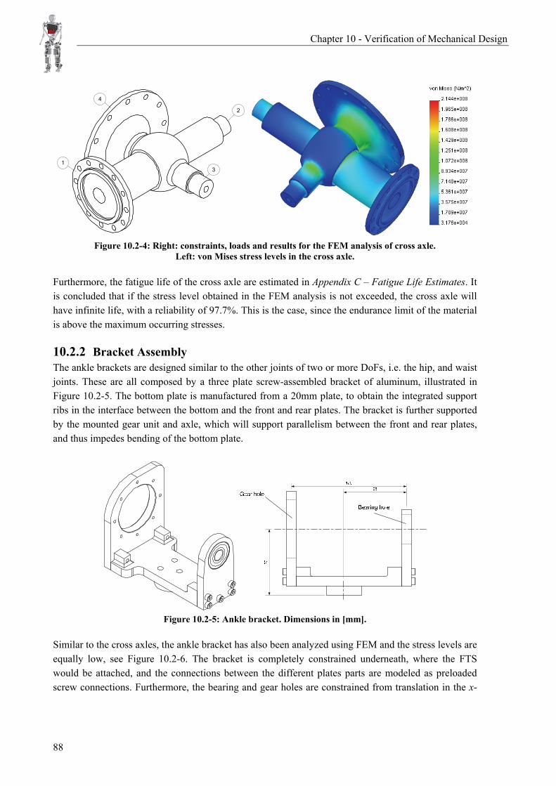
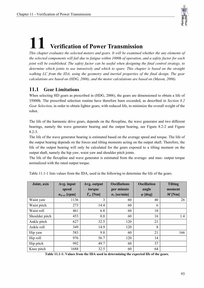
10 Verification of Mechanical Design................................................................................................... 83 10.1 Construction Materials ......................................................................................................... 83 10.2 Case Study: Ankle................................................................................................................ 84 10.3 Summary .............................................................................................................................. 91

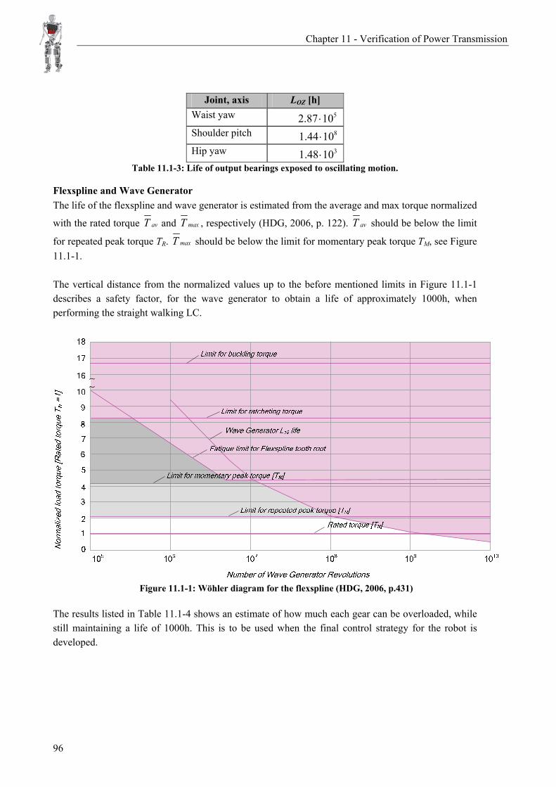
11 Verification of Power Transmission................................................................................................. 93 11.1 Gear Limitations .................................................................................................................. 93

11.2 Motor Limitations ................................................................................................................ 97 11.3 Summary............................................................................................................................ 100

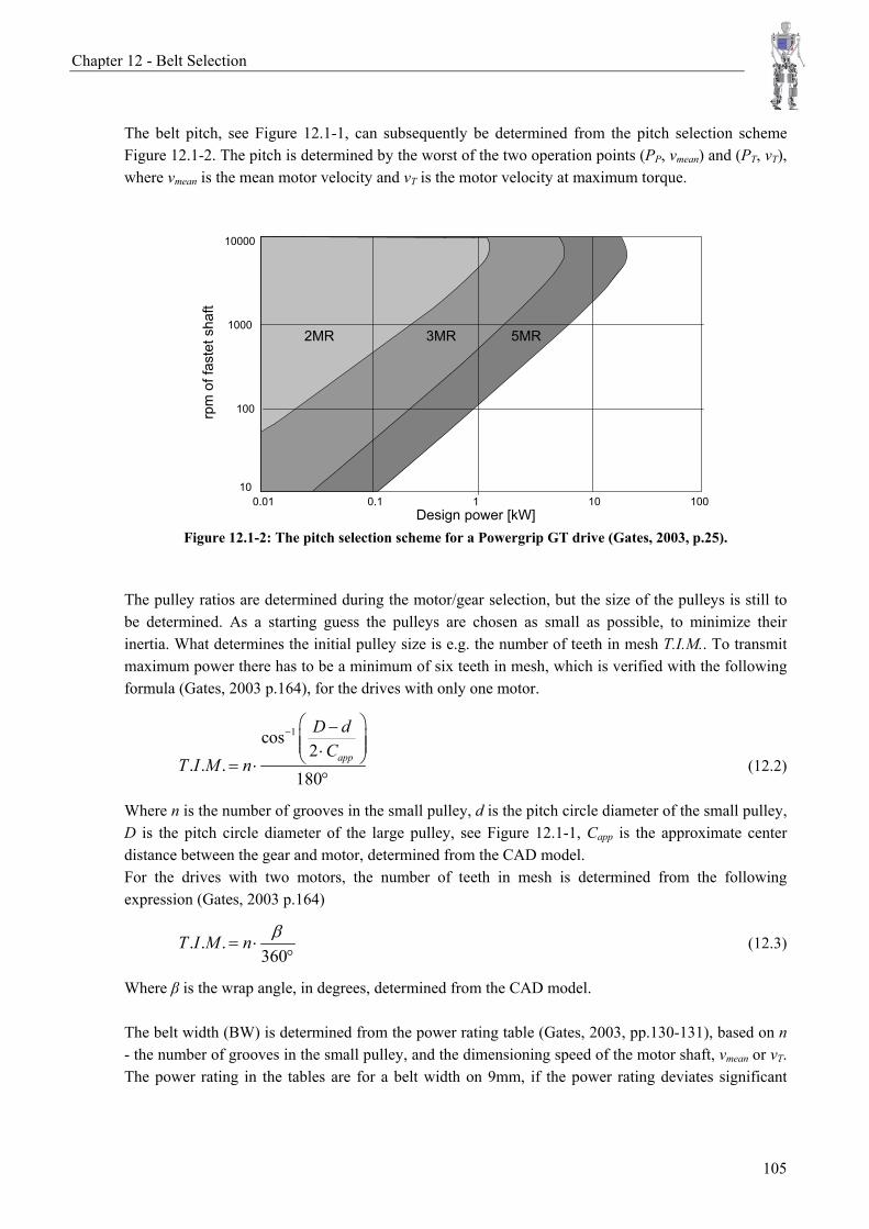
12 Belt Selection ................................................................................................................................. 103 12.1 Belt Types.......................................................................................................................... 103 12.2 Summary............................................................................................................................ 109

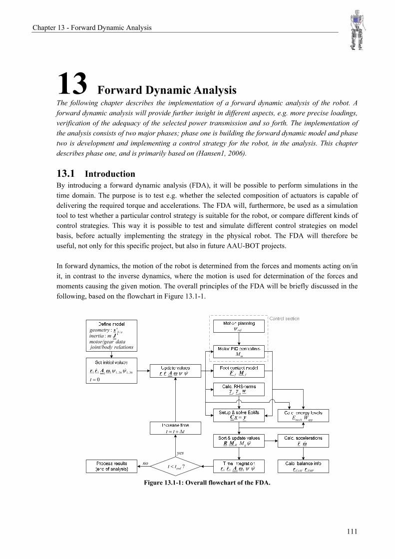
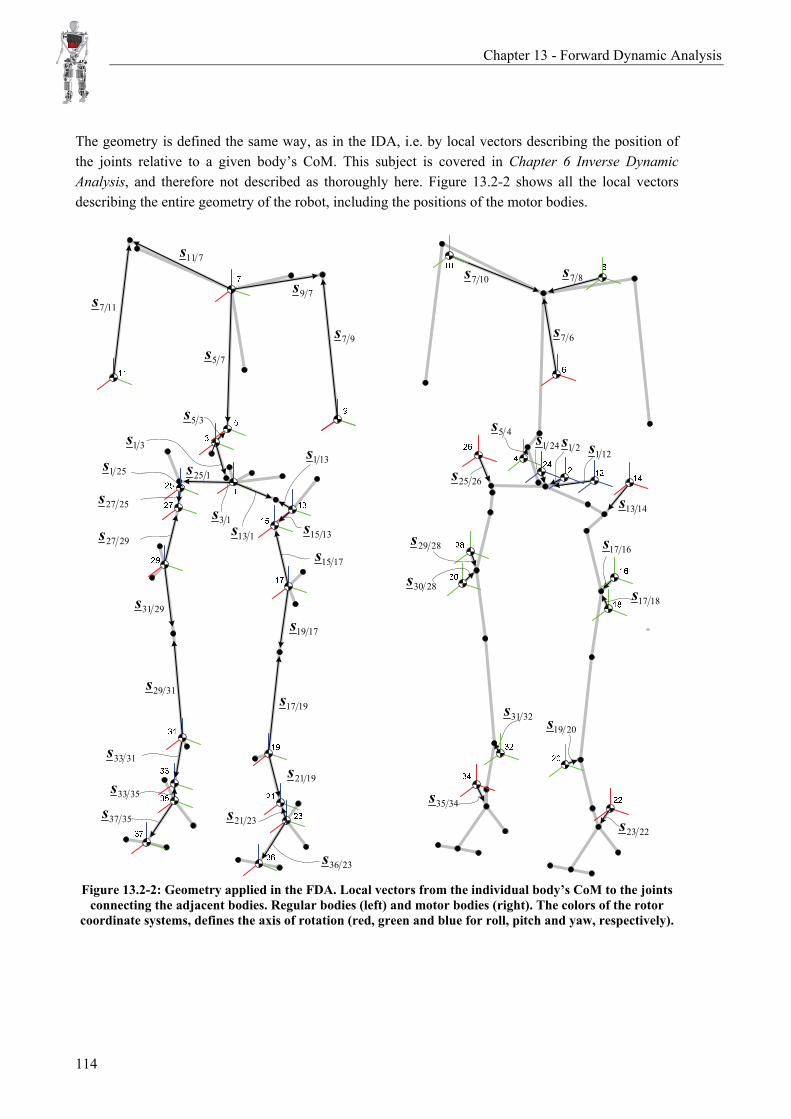
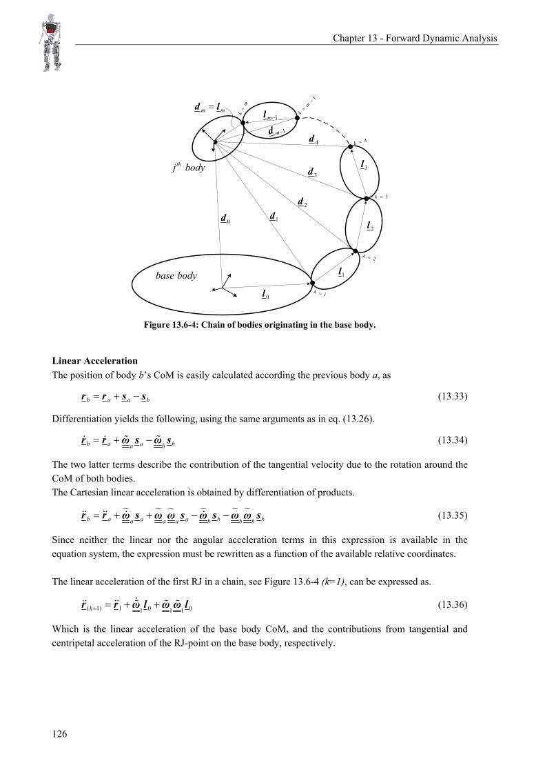
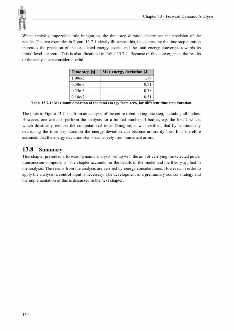
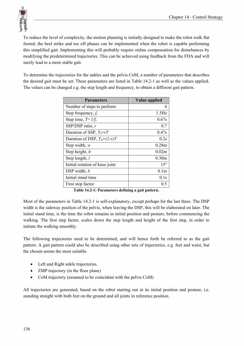
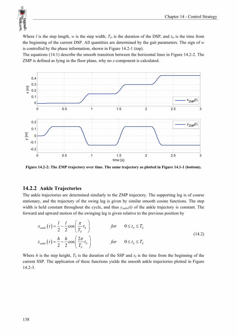
13 Forward Dynamic Analysis............................................................................................................ 111 13.1 Introduction........................................................................................................................ 111 13.2 Model Definition................................................................................................................ 112 13.3 Relative Coordinates.......................................................................................................... 115 13.4 Kinematics ......................................................................................................................... 116 13.5 Foot Contact Model ........................................................................................................... 118 13.6 Setting Up and Solving Equations of Motion .................................................................... 121 13.7 Energy Balance .................................................................................................................. 131 13.8 Summary............................................................................................................................ 134

14 Control Strategy ............................................................................................................................. 135 14.1 Overview of Control Strategy............................................................................................ 135 14.2 Offline Motion Planning.................................................................................................... 135 14.3 Online Control ................................................................................................................... 146 14.4 Implementing Controls in the FDA ................................................................................... 150 14.5 Evaluation of the FDA and Control Strategy..................................................................... 152 14.6 Summary............................................................................................................................ 153

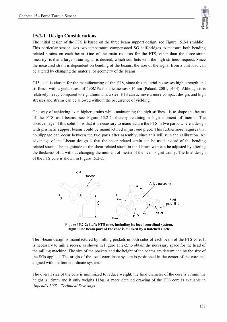
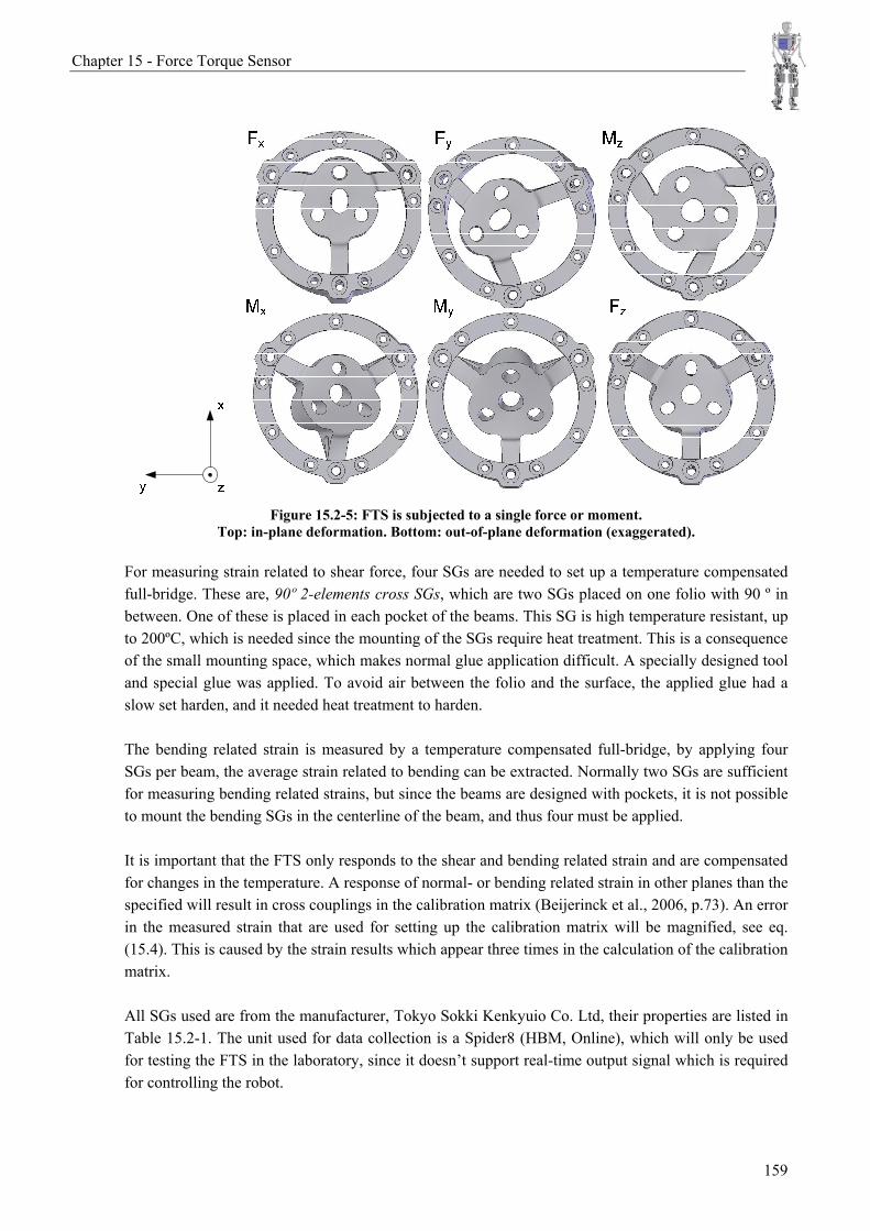
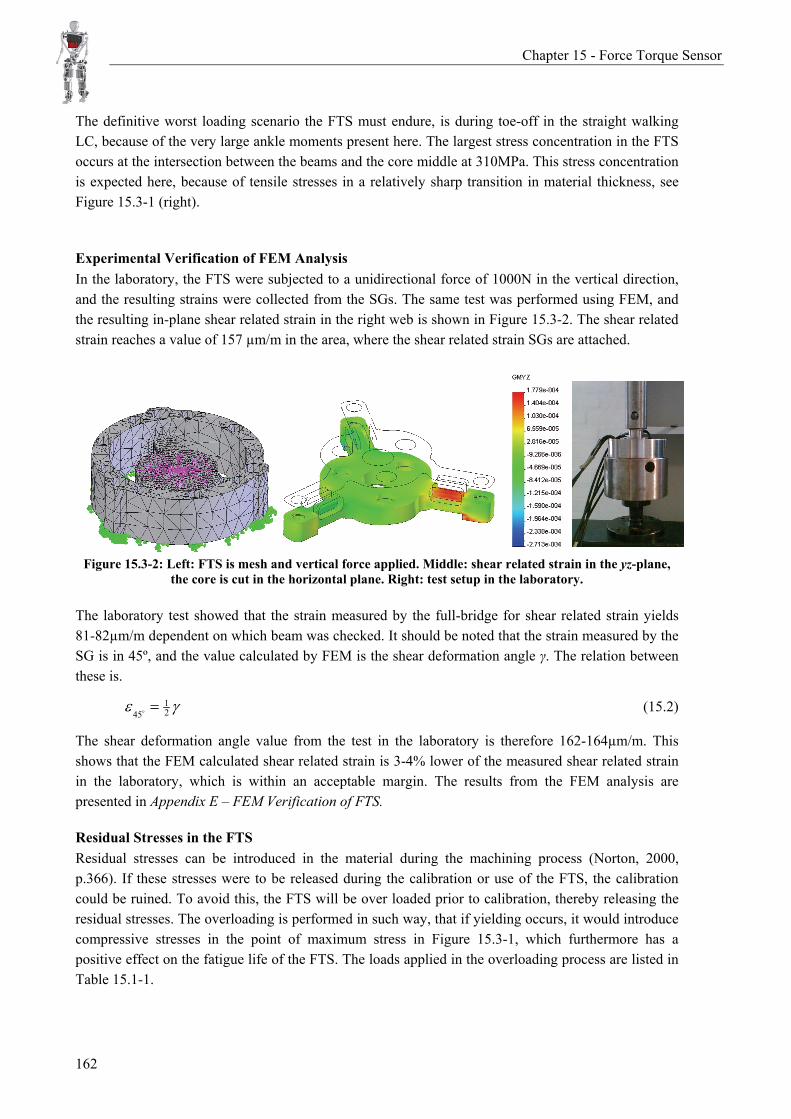
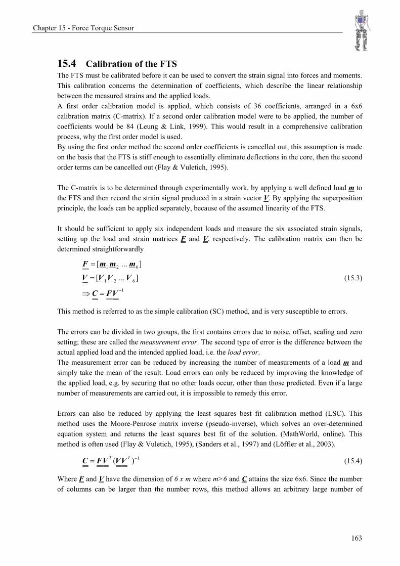
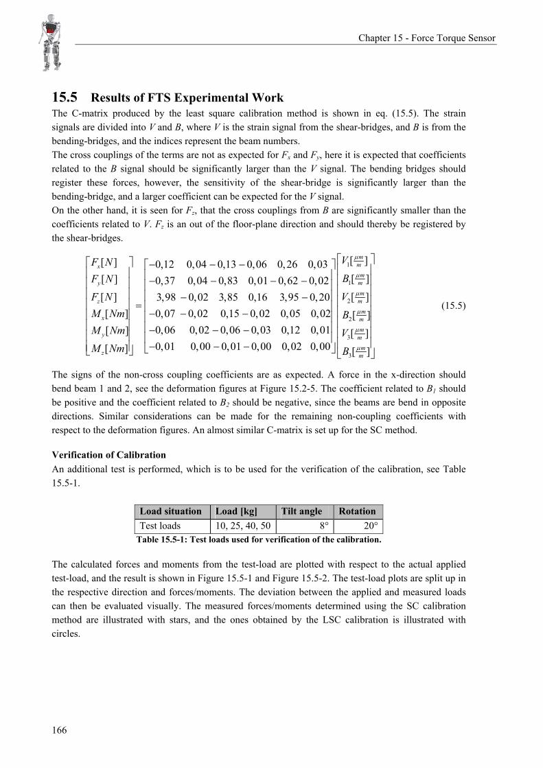
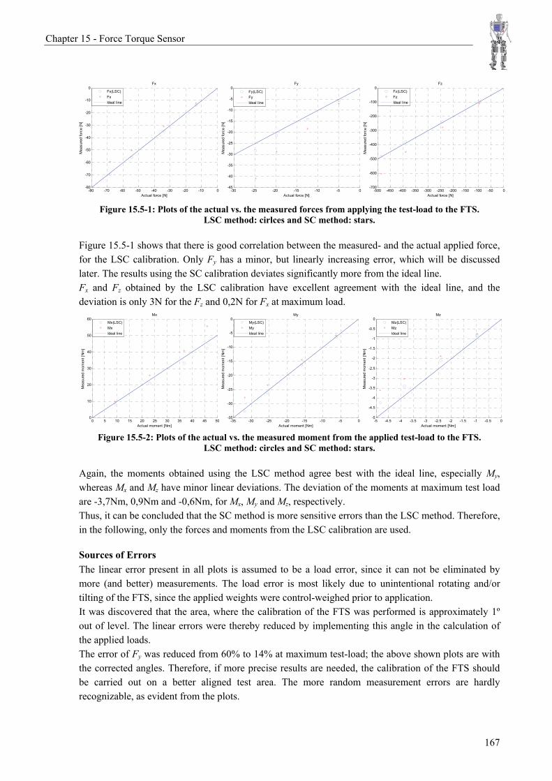
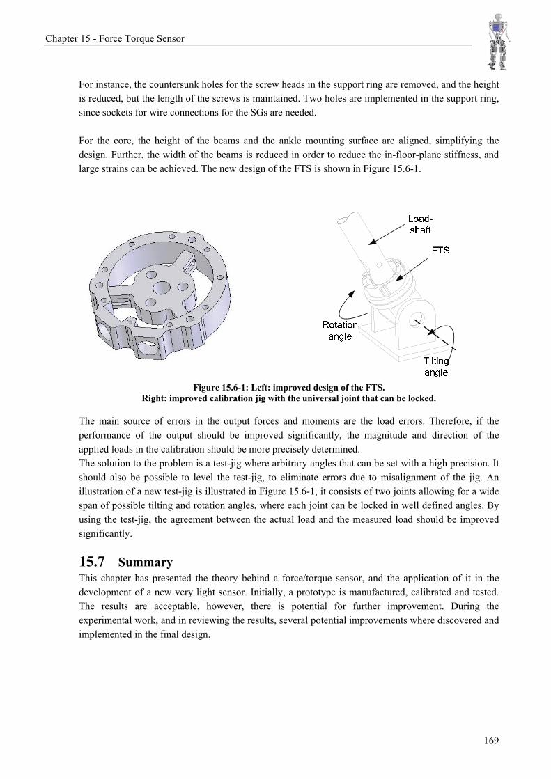
15 Force Torque Sensor ...................................................................................................................... 155 15.1 Purpose .............................................................................................................................. 155 15.2 Design of the Six Axis FTS ............................................................................................... 156 15.3 FEM Verification of the FTS............................................................................................. 161 15.4 Calibration of the FTS ....................................................................................................... 163 15.5 Results of FTS Experimental Work................................................................................... 166 15.6 Improvements and Final Design ........................................................................................ 168 15.7 Summary............................................................................................................................ 169

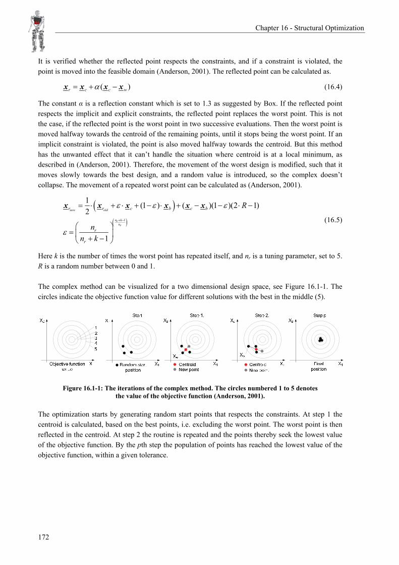
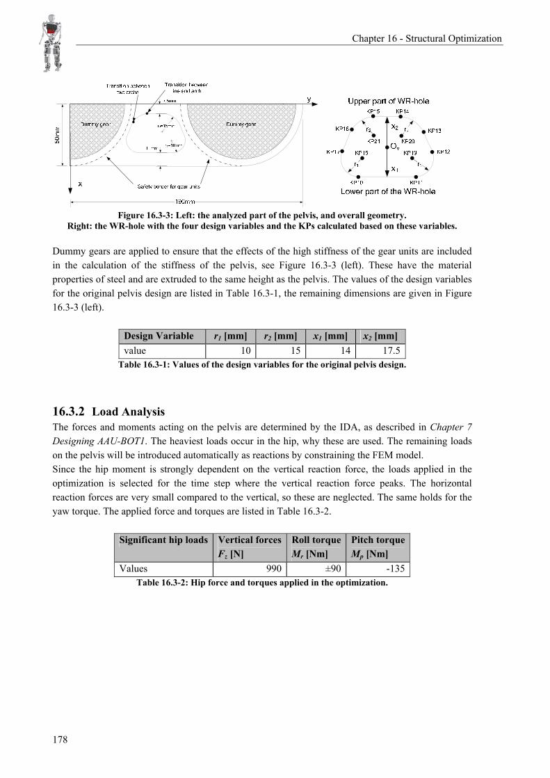
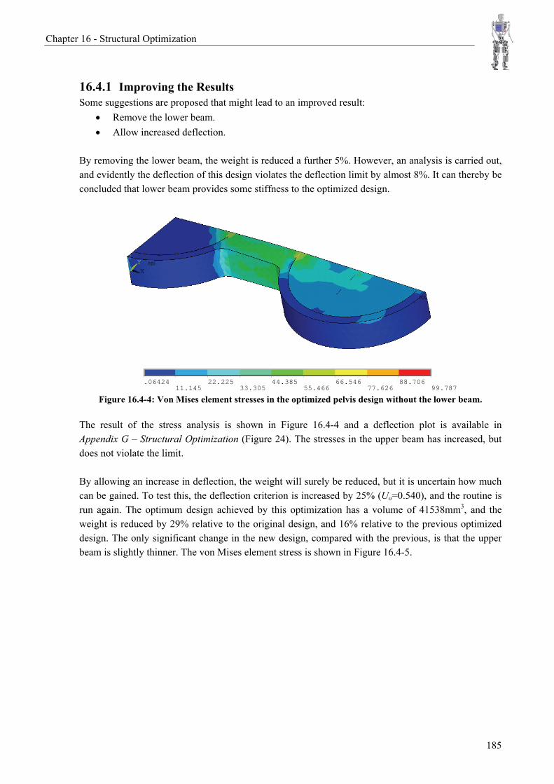
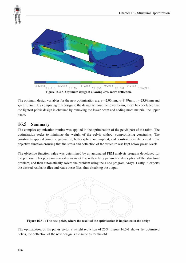
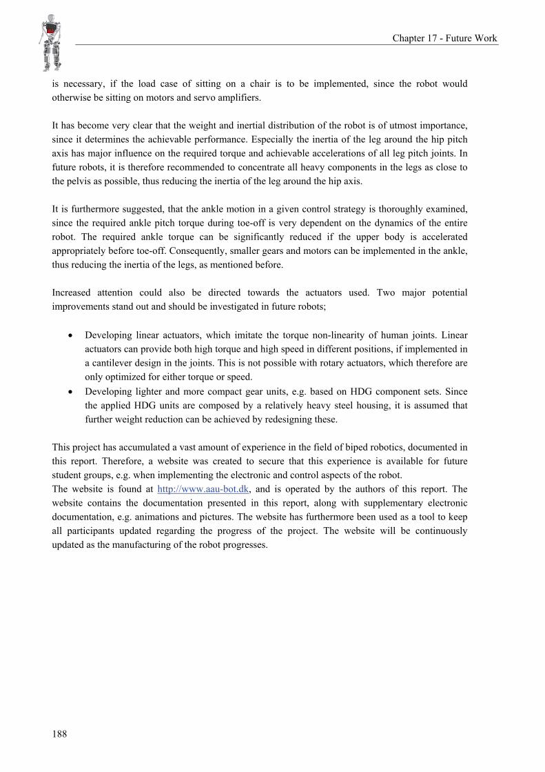
16 Structural Optimization .................................................................................................................. 171 16.1 The Complex Method ........................................................................................................ 171 16.2 Implementing the Complex Routine.................................................................................. 173 16.3 Optimization of the Pelvis ................................................................................................. 175 16.4 Results From the Pelvis Optimization ............................................................................... 182 16.5 Summary............................................................................................................................ 186

17 Future Work ................................................................................................................................... 187 18 Conclusion...................................................................................................................................... 189 19 References ...................................................................................................................................... 191

Chapter 1 - Introduction

1

1 Introduction Biped robots have been an interesting research topic for many years, especially in Japan where studies in this field have been conducted for more than 40 years. Recent developments in actuators, sensors and computers have enabled the realization of more and more sophisticated anthropomorphic biped robots. The state of the art biped robots, e.g. Honda’s ASIMO, Waseda University’s WABIAN-2 or TUM’s Johnnie, is capable of fairly human-like walking, even running in the case of ASIMO. However, their gait is comparable to that of an old human with back pain. All of them walk somewhat slowly, only up to about 3km/h, and with their feet flat on the floor. In order to enter this scientific field AAU has initiated the development of its own anthropomorphic biped robot, named AAU-BOT1, which will also be referred to in this text as the robot. This first robot should serve to gain insight in the field, and form a basis for further research, i.e. be a launch pad for future anthropomorphic biped robots. Although the project budget is limited to 500.000DKK, the project has other advantages, primarily in the form of free labor, both for design and manufacturing, and a vast amount of expertise available. Additionally, after developing AAU-BOT1, fundraising for further projects in this field should be easier.

1.1 Goals and Objectives The goal of the AAU-BOT1 project is to develop and manufacture a dynamic walking biped robot of human proportions. While it is optimistic to develop a robot which is overall more sophisticated than the previously mentioned, because of time and budget limitations. The novelty and differentiation from other projects is to be realized via a more human-like gait, so-called dynamic walking. This project concerns the development of the mechanics of the AAU-BOT1; this includes the structural parts as well as the mechanical and electrical power transmissions. The robot should be able to imitate dysfunctional walking e.g. limping, however this is only to be implemented through control. When the mechanical design is complete, other projects dealing with control and electronics will be initiated, by other student groups. The main feature of the AAU-BOT1 should be the realization of a more human like gait than seen before in existing biped robots. This should be achieved through the implementation of heel-strike and toe-off capabilities in the feet. This will be elaborated on later, but basically means not walking with the feet flat on the floor. Another point, where the AAU-BOT1 stands out is that it will be developed by students only, something that hasn’t been done before. In lay terms, this first robot should serve as a beginning, from which experience can be harvested, so that in the future, more sophisticated robots can be developed at AAU.


2

1.2 Definition of Work The main tasks and work flow of this project is outlined in the following. The introductory parts comprise an introduction of the state of the art existing biped robots, and a survey is presented for inspirational purpose. Furthermore, an analysis of the human gait is conducted, in order to achieve the necessary understanding of gait kinematic , dynamics and the terminology used in this field. The introductory part is concluded by the definition of a requirements specification, which is set up in collaboration with all the participants of the AAU-BOT project, see Appendix L – Project Participants. The kinematics of human gait is thereafter obtained experimentally by means of motion capture facilities. Based on these data, a fair estimate of the loads acting on the robot can be established, using inverse dynamic modeling. The obtained loads are sorted and the dimensioning loads are emphasized. These loads, especially the joint torques, are then utilized in the power transmission design, for selection of motors, servo amplifiers and gears. Knowing the dimensions of these components, the load-carrying structure can then be designed and its adequacy verified. This process is somewhat iterative due to the many unknown dependent factors. This phase is concluded by documenting the design via technical drawings and initiation of the manufacturing and subsequent assembly of the robot. Since the power transmission components are discrete design components, a compromise is made in the selection of these, such that some joints are under-powered and some are over-powered. This is done in order to reduce the overall weight of the robot and to ensure surplus power to handle unforeseen control issues. Because of the redundancy of the robot, this can easily be compensated for by using the different joints smartly. Therefore, limitations for the final control strategy for the robot are set up, thus clarifying which joints to use intensively and which to spare, this information is especially useful for future students that are to develop the final control of the robot. To verify whether the selected actuators are capable of making the robot walk, a detailed forward dynamic analysis is performed. This provides a simulation environment, in which different aspects can be investigated. To make the robot perform a walking cycle in the forward dynamic analysis, it is necessary to implement a control strategy. This analysis can also be a powerful tool in future student projects, e.g. to test a developed control strategy. To obtain a force feedback from the feet, a six-axis force/torque sensor is developed and implemented in the physical robot. This is of major importance for the final control strategy. Furthermore, weight reduction is sought by developing a scheme for shape optimization of the structural parts. This scheme is applied to one of the heavier parts, for testing and verification.


3

Project Work Flow • Research and map existing biped robots. • Establish requirements specification. • Analyze human gait and anatomy. • Obtain human gait kinematics. • Determine loads. • Design power transmission. • Design mechanism. • Verify mechanical and power transmission design. • Create technical drawings and commence manufacturing. • Determine control limitations to ensure lifespan. • Build simulation environment, for further analysis and verification. • Develop and implement preliminary control strategy in simulation. • Develop six-axis force/torque sensor. • Reduce weight by shape optimization.

The work flow is illustrated schematically in Figure 1.2-1. As evident some iteration are necessary during the selection of power transmission components and mechanical design phases, since they are highly inter-dependent.

Figure 1.2-1: Work flow, PT denotes power transmission.

Furthermore, because of the wide span of tasks, it has not been possible to maintain a strict chronological order of the treatment of subjects in the report. This is also illustrated in Figure 1.2-1, where e.g. the belt drive selection and force/torque sensor development is not necessary for the further work, but still required in the final robot.

Chapter 2 - Existing Biped Robots

5

2 Existing Biped Robots This chapter describes and evaluates three advanced biped robots. This is a small, but representative collection of the existing biped robots, using servo motors as actuation. The overall features, degrees of freedom (DoFs), performance and certain soft- and hardware aspects will be discussed. However, the scope of this chapter is to investigate the mechanical design and power transmission specifications of existing robots, such to achieve inspiration for the design of AAU-BOT1. This chapter is based on (ASIMO, Online), (WABIAN, Online), (Johnnie, Online) and (Wollherr, 2005).

2.1 Presentation The three selected biped robots are ASIMO, WABIAN-2 and Johnnie, see Figure 2.1-1. They give a good impression of what is achievable of a biped robot at this time, and how different technical solutions can be obtained. Since there are no detailed technical drawings or part lists available, the technical solutions and performance are evaluated from online photos and video clips. Honda’s ASIMO is covered by a plastic shield, which complicates the investigation. The non-corporate WABIAN-2 and Johnnie, however is not, hence the description of these will be more thorough. The technical specifications for the three robots are listed in Appendix A – Technical Data for the Existing Robots.

Figure 2.1-1: Left: ASIMO, Middle: WABIAN-2 and Right: Johnnie (not same scale).


6

ASIMO ASIMO is developed by the Honda motor company. The research started in 1986, and the first humanoid robot P1 was introduced in 1993. On the success of the P- robots, ASIMO was introduced in year 2000, and a number of updates have followed since, including one capable of running at 3km/h in 2004. In 2005 the model new ASIMO, which is often referred to as the state of art biped robot, was introduced. It is capable of straight running at 6km/h and circling at 5km/h. Furthermore, ASIMO is completely autonomous, can turn when walking and climb stairs. During turning, the center of mass (CoM) is shifted to the inside of the turn and the length of the inner leg is decreased with respect to the outer leg. To obtain human-like walking, ASIMO has soft projections under its feet which imitate toes. Aside from walking and running, ASIMO understands spoken commands and recognizes human faces.

WABIAN-2 Waseda University, started researching biped robots in 1966, and published their first humanoid robot in 1973. Since then, a number of biped robots have been developed, concluded by WABIAN-2 in 2003. This biped robot differs from ASIMO and Johnnie because of its 41 DoFs, which is more than twice that of Johnnie, and eight more than ASIMO. Extra DoFs in the ankles allow moving the knees sideways, when both feet are fixed on the ground and reduce the impact force due to heel strike, when walking on rugged terrain (Lim et al, 2005). Extra DoFs in the torso allows for walking with stretched knees, due to independent orientation of the trunk (WABIAN, Online). These extra DoFs support a more smooth human-like walk.

Johnnie The Johnnie robot was developed at the Technical University of Munich to initiate research in bipedal walking. Johnnie was built for the German Research Foundation in the Priority Program Autonomous Walking. This program started in 1998, with the intention to create a human-like dynamically stable gait for a humanoid robot. Johnnie can pass obstacles on its gait trajectory, e.g. step over or step onto. This is achieved by a visual guiding system, based on a stereo camera system. Johnnie is a European built biped robot, whereas ASIMO and WABIAN-2 are made in Japan, where most research in biped robotics are conducted.

2.2 Mechanical Design The mechanical designs to be investigated are divided into the segments; foot/ankle, knee, hip and waist. Honda has released a low resolution video clip of ASIMO, without the plastic shield, which makes it possible to examine the knee and ankle designs.

Foot/Ankle The ankles are constructed in two different ways. ASIMO and WABIAN-2 use Harmonic Drive gears (HDG) with a belt drive connection to DC servo motors (SM), whereas Johnnie uses a ball screw system. ASIMO has two DoFs (roll, pitch) in the ankle, and WABIAN has three, see Figure 2.2-2, this gives ASIMO the advantage of a lighter foot compared to WABIAN. Furthermore, ASIMO’s ankle pitch SM is located near the knee; see Figure 2.2-4 (left), which lowers the inertia of the shin around the knee axis, but requires a long belt drive. It is desirable to keep the inertia of the legs at a minimum to reduce the joint torque requirements (Huang et al., 2001). On the other hand, three DoFs in the ankle can provide a more human-like walk, and a shorter belt drive yields less backlash.


7

Johnnie has two DoFs in the ankle, but applies a ball screw gear (BSG) system instead. This gives the advantage that the ankle SMs can be placed near the knee, without the undesirable backlash of a belt drive connection. Johnnie has two BSGs on each leg, see Figure 2.2-3, where the system is illustrated for Johnnie’s right foot. Furthermore, an illustration from behind of the next generation of Johnnie, LOLA shows the same system. The BSG system enables pitch and roll rotation of the ankle by SM rotation the same, and opposite ways, respectively. This joint actuator operates very similar to the human muscle, which potentially could provide a more human-like walk, although the joint torque produced will be nonlinear.

Ankle pitch

Ankle roll

Ball screw

Figure 2.2-1:

ASIMO; 2 DoFs. Figure 2.2-2:

WABIAN-2; 3DoFs Figure 2.2-3: Right: Johnnie; 2DoFs BSG.

Left: LOLA; 2 DoF ankle, 1DoF toes. Most biped robots observed applies quite large feet compared to humans, especially the width are out of proportions, but apparently necessary in order to maintain sideway balance. None of the observed existing robots incorporates toes, since they are unnecessary when walking flat-footed. The foot is an essential part for human-like walking, as mentioned earlier ASIMO has soft projections under the feet that can absorb the impact and can be controlled to imitate the effect of toes. Johnnie’s feet are designed with four point ground contacts with integrated damping. The Johnnie group wanted sophisticated foot dynamics, but didn’t achieve it, because of the lack of toes. This problem is taken into consideration in their next generation robot LOLA, where toes has been implemented, see Figure 2.2-3 (right).

Knee All three robots apply similar actuation of the knees, which consists of a HDG and a SM with a belt drive connection. The SM on ASIMO is located near the hip which lowers the inertia of the thigh, where the two other robots have the SM installed near the knee, see Figure 2.2-4. ASIMO is the only of the three robots capable of running, which necessitates low inertia legs, when swinging them rapidly. The load carrying structure of ASIMO is mainly based on cast magnesium alloy, where Johnnie and WABIAN primarily employ milled high strength aluminum.


8

Figure 2.2-4: Knee design of the robots. Left: ASIMO, Middle: WABIAN-2 and Right: Johnnie.

Hip The human hip is a spherical joint, which is reproduced in all three robots by a 3 DoF joint. No photos of ASIMO’s hip construction are available, but it is assumed to be similar to that of WABIAN. All three axes of WABIAN’s hip construction are intersecting in the same point; see Figure 2.2-6. This means that no extra joint torque is required to counteract a moment introduced by an offset joint axis. The hip construction in Johnnie has a slightly offset pitch axis, see Figure 2.2-5 left. Since the human hip is a spherical joint, it is assumed that the most human like gait is achieved by implementing a joint with intersecting axes, although production of such joint might be more challenging due to the very compact design required. It should be noted that Johnnie applies two DC motors, connected to one HDG at the hip pitch axis. Thereby, two small motors can be used instead of one larger motor, since this yields a higher performance-to-weight-ratio (Gienger et al., 2000). A better illustration of the concept is found in the Korean made robot KIAST; see Figure 2.2-5. Furthermore, 3 DoF hips are assumed necessary for turning a robot properly.

Figure 2.2-5: Left: a detail view of Johnnie’s hip. Right: Thigh of the KAIST robot (Park et al., 2003).

Figure 2.2-6: WABIAN’s hip and pelvis

construction (Ogura, 2006).


9

Waist/Trunk ASIMO do not include a waist joint, and Johnnie has only one DoF in the waist and no trunk joint. Johnnie has a yaw axis, which allows rotation around vertical of the torso relative to the pelvis. The next generation of Johnnie (LOLA), has five DoFs more than Johnnie, one of which is located in the waist, see Figure 2.2-8, which adds the possibility to roll the torso independently. WABIAN has two DoFs in the waist and two in the trunk. The waist joint can roll and yaw and the trunk can roll and pitch, see Figure 2.2-7. The torso can therefore rotate completely independent from the lower part of the body. However, the redundancy of having two roll axes between the torso and pelvis is not clear. Since humans have a very flexible connection between the pelvis and the torso, composed by the spine, it seems necessary to implement at least 3DoFs in this joint.

Figure 2.2-7: DoF illustration for WABIAN-2. (WABIAN, Online).

Figure 2.2-8: DoF illustration for LOLA, red axes marks additions to Johnnie (Johnnie, Online).

2.3 Summary This chapter has introduced three of the leading biped robots that exist today. Though the robots are all based on human beings, the technical solutions and the number of DoFs varies greatly. The state of the art biped robot use DC servo motors primarily connected to Harmonic Drive gears by belt drive connections. It has in the vicinity of 6 DoFs per leg and 1-3DoFs in waist, arms and hands are not considered as relevant at this stage. The robots walks relatively slow, i.e. less than 1m/s, they all walk with their feet flat on the floor, ASIMO even has the ability to run this way. They naturally seek a very light, stiff and strong construction, in order to increase controllability and reduce power consumption and actuator size. The current robot’s main ability is walking, interaction with the environment using arms and hands still remains to be implemented properly. However, a prerequisite of this, is that overall stability needs improving.

Chapter 3 - Human Gait and Anatomy

11

3 Human Gait and Anatomy This chapter presents a brief investigation of human gait and anatomy. The different phases and events of the walking cycle will be explained, and definitions used throughout this report will be introduced. The purpose of this chapter is to obtain the necessary understanding of the subject needed in the load determination and design phases. The chapter is mainly based on (Vaughan et al., 1999) and (Inman et al., 1981).

3.1 Definitions In this section the terminology, regarding human gait and anatomy, used in the report will be defined in order to eliminate ambiguities. Firstly the robot parts will be defined. Some of the definitions in Figure 3.1-1 might seem obvious, but all names are presented in order to clarify which are regarded as body parts and joints, respectively.

Shoulder

Waist

Hip

Knee

Ankle

Torso

Arm

Pelvis

Thigh

Shin

Foot

Toe joint

Toe

Joints: Bodies:

Figure 3.1-1: Right: Definition of body parts and joints used in this report.

Left: Planes and orientation of main coordinate system used in this report. (Inman et al., 1981, p.34) Figure 3.1-1 illustrates the primary coordinate system orientation and associated planes used in this report. Furthermore, it seems that the literature on biped robotics has adopted the terminology of flight dynamics, i.e. roll, pitch and yaw means rotation about the x, y and z-axes respectively.

3.2 Human Gait Gait can be defined as periodic movement of the legs, called steps, making up a complete cycle of walking. This cycle can be divided into two primary and eight secondary phases as illustrated in Figure 3.2-1 and Figure 3.2-2. By convention, the cycle is set to begin with the right heel touching the ground.


12

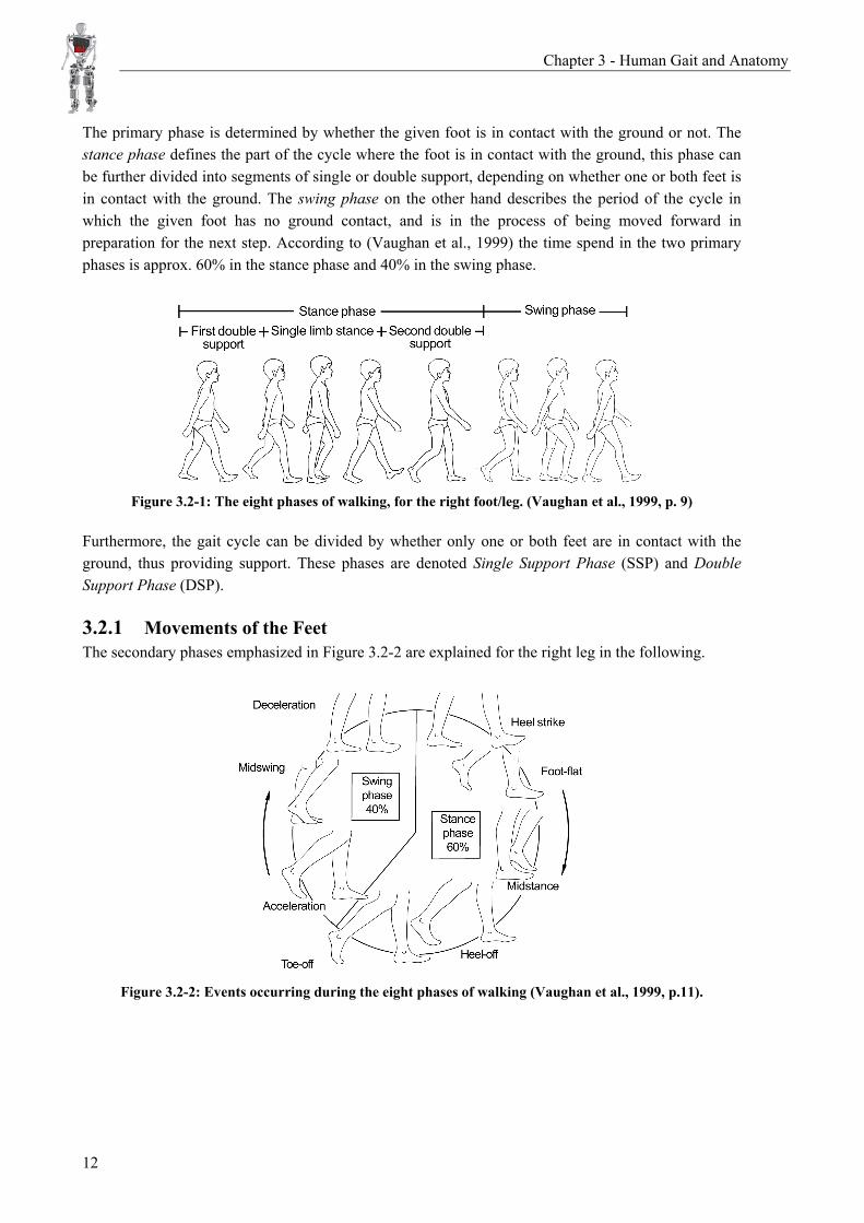
The primary phase is determined by whether the given foot is in contact with the ground or not. The stance phase defines the part of the cycle where the foot is in contact with the ground, this phase can be further divided into segments of single or double support, depending on whether one or both feet is in contact with the ground. The swing phase on the other hand describes the period of the cycle in which the given foot has no ground contact, and is in the process of being moved forward in preparation for the next step. According to (Vaughan et al., 1999) the time spend in the two primary phases is approx. 60% in the stance phase and 40% in the swing phase.

Figure 3.2-1: The eight phases of walking, for the right foot/leg. (Vaughan et al., 1999, p. 9)

Furthermore, the gait cycle can be divided by whether only one or both feet are in contact with the ground, thus providing support. These phases are denoted Single Support Phase (SSP) and Double Support Phase (DSP).

3.2.1 Movements of the Feet The secondary phases emphasized in Figure 3.2-2 are explained for the right leg in the following.

Figure 3.2-2: Events occurring during the eight phases of walking (Vaughan et al., 1999, p.11).


13

Stance Phase: • The cycle begins in the stance phase with heel strike of the right foot, thus achieving the initial

contact with the ground. At this point the CoM is at its lowest vertical position. Note that the impact force of heel-strike does not produce high ankle moments, since there is almost no arm for the force to act in.

• Secondly the right foot rolls over in what is called foot flat, so that the entire right foot is now in contact with the ground, and the left is preparing to enter its swing phase.

• Then the left foot swings past the right, which is called midstance, it also marks the point at which the CoM is at its highest vertical position. The right foot remains flat on the ground.

• Subsequently at heel-off, the right heel looses contact with the ground as the foot rolls up upon the toes, by pitch rotation in the ankle.

• The last event of the stance phase is called toe-off, which occurs when the right foot completely looses contact with the ground.

Swing Phase: • The swing phase starts with the angular acceleration of the entire leg around the hip pitch aics

as soon as the foot loose contact with the ground. • Then midswing occurs when the right foot swings past the left, which is currently in

midstance. • Lastly deceleration of the foot occurs, which prepares for the next heel strike, and a new

cycle.

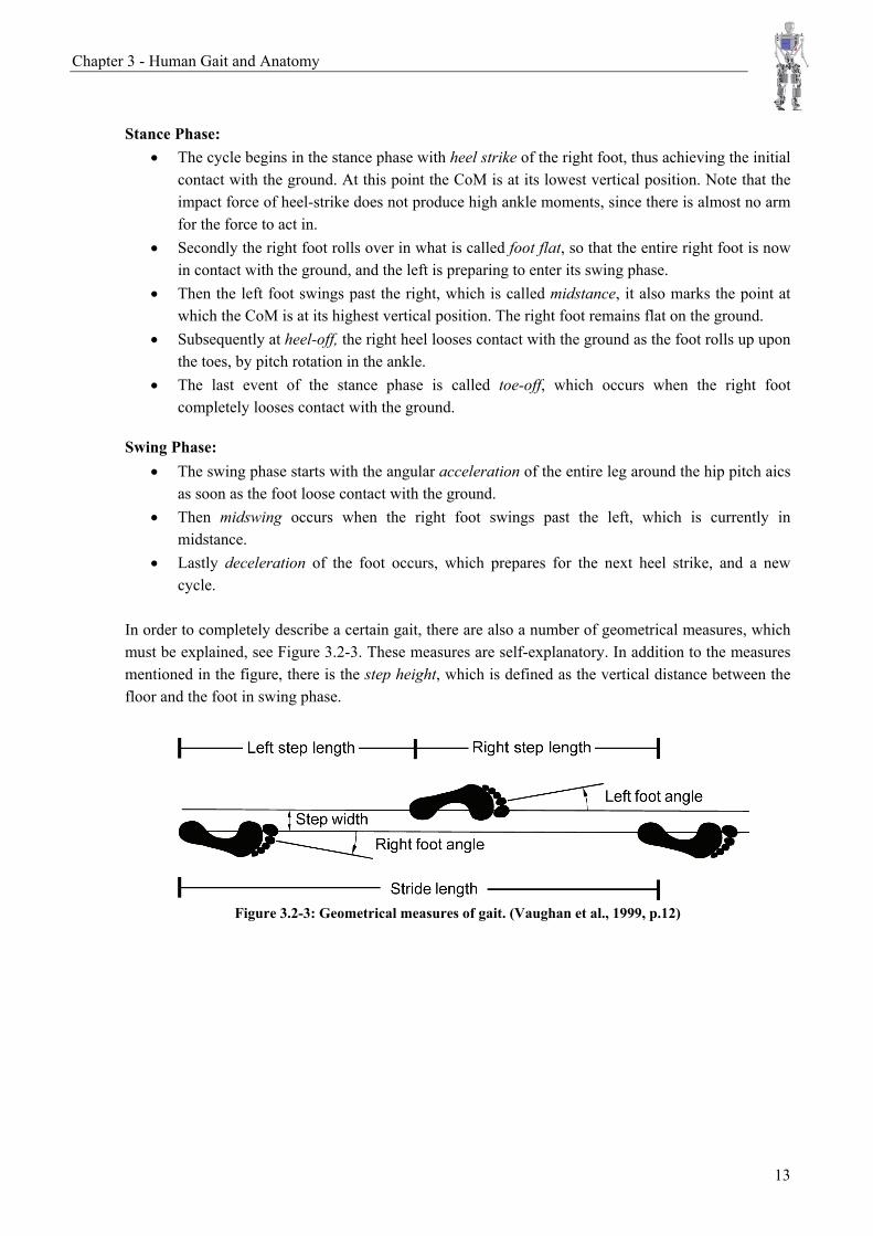
In order to completely describe a certain gait, there are also a number of geometrical measures, which must be explained, see Figure 3.2-3. These measures are self-explanatory. In addition to the measures mentioned in the figure, there is the step height, which is defined as the vertical distance between the floor and the foot in swing phase.

Figure 3.2-3: Geometrical measures of gait. (Vaughan et al., 1999, p.12)


14

3.2.2 Movements of the Body This section is based on (Inman et al., 1981, pp.2-22). All major body parts move during walking; the legs, the pelvis, the torso and the arms. These movements will be described in the following.

• Pelvic rotation describes the rotation of the pelvis around the yaw axis. The rotation is approximately 4° to the right and 4° to the left alternately under normal walking conditions. This effect elongates the step length.

• Pelvic list describes the tendency of the pelvis to list downward in the non-weight bearing

side. This results in an angular displacement of approximately 5° in the frontal plane, i.e. around the roll axis. The displacement occurs in the hip joints. Because of the pelvic list, the non-weight bearing leg must contract itself, by flexing the knee, in order to steer free of the ground during the swing phase.

• Knee flexion in stance phase. During heel-strike the knee of the supporting leg is almost

straight, but it begins to flex until the foot is flat on the ground. This flexion is equivalent to a rotation of approximately 15° in the knee. The knee flexion both absorbs some of the impact of the heel-strike as well as decreases the elevation of the center of mass.

• Sideway displacement of the body. During the stance phase the entire body shifts slightly over

the weight bearing leg. The magnitude of this shifting is about 4-5cm per stride, depending on the step width. This motion is maintained by rotation about the roll axis of the hip and ankle.

• Rotations in the transverse plane; i.e. yaw. Apart from the pelvic rotation, the body also

rotates in the transverse plane in the following locations.

o Rotations of the torso. During walking the torso rotate 180° out of phase with the pelvic rotation, in the waist. This causes swinging motion in the arms. When a leg swings forward, the opposite arm simultaneously swings forward.

o Rotations of the thigh and shin. The lower parts of the legs rotate in phase with the

pelvis, but the rotation increases from the pelvis to shin. The bottom of the shin rotates approximately 15° relative to the pelvis. The legs rotate inwards from the beginning of the swing phase until midstance, where the outwards rotation commences.

o Rotations in the ankle and foot. The ankle joint and the foot, contain mechanisms that allow for rotation of the leg, while keeping the foot stationary during the stance phase, thus absorbing the rotation. This is possible through many complex flexible joints in the foot and ankle.


15

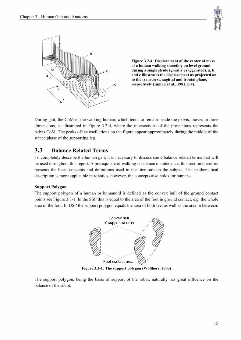
Figure 3.2-4: Displacement of the center of mass of a human walking smoothly on level ground during a single stride (greatly exaggerated). a, b and c illustrates the displacement as projected on to the transverse, sagittal and frontal plane, respectively (Inman et al., 1981, p.4).

During gait, the CoM of the walking human, which tends to remain inside the pelvis, moves in three dimensions, as illustrated in Figure 3.2-4, where the intersections of the projections represents the pelvis CoM. The peaks of the oscillations on the figure appear approximately during the middle of the stance phase of the supporting leg.

3.3 Balance Related Terms To completely describe the human gait, it is necessary to discuss some balance related terms that will be used throughout this report. A prerequisite of walking is balance maintenance, this section therefore presents the basic concepts and definitions used in the literature on the subject. The mathematical description is more applicable in robotics, however, the concepts also holds for humans.

Support Polygon The support polygon of a human or humanoid is defined as the convex hull of the ground contact points see Figure 3.3-1. In the SSP this is equal to the area of the foot in ground contact, e.g. the whole area of the foot. In DSP the support polygon equals the area of both feet as well as the area in between.

Figure 3.3-1: The support polygon (Wollherr, 2005)

The support polygon, being the basis of support of the robot, naturally has great influence on the balance of the robot.


16

Center of Mass & Ground Projection The center of mass of a number of bodies, the CoM, is a well known term; the position vector of rCoM is calculated as follows

1

1

b

b

niii

CoM nii

m

m=

=

= ∑∑

rr (4.1)

Where mi is the mass of the ith body of the robot and ri is the position of the ith body’s CoM. The ground projection of the center of mass (GCoM) is the orthogonal projection on the floor. The position of the GCoM determines whether a motionless robot is balanced, i.e. if the GCoM falls within the support polygon, the robot is balanced. This means that the gravity forces exerted on the robot does not produce any tilting moments around the ground contact.

Zero Moment Point The zero moment point (ZMP) is the dynamic equivalent of the GCoM. It is the point on the ground where the total external reaction force has to act, to completely balance the robot. At this point both reaction moments about the horizontal axes equals zero, hence the name zero moment point. Likewise the ZMP determines whether a moving robot is in balance

Sagittal plane Frontal plane

im g im g

, ,i y i yJ ω

, ,i x i xJ ωi im x

i im zi im z

i im y

,T zR

iz iz

iyix

ZMPx,T zRZMPy

yx

z

yx

z

x

z

yx

z

y

Figure 3.3-2: Free body- and kinetic diagrams for calculation of the ZMP. The appropriate terms for the ith body is illustrated at the overall CoM.

The position of this point is determined by demanding moment equilibrium around origin in the sagittal and frontal planes respectively, this way one can determine first the x-position and then the y-position of the point. For illustration, the calculation of the x-position is shown here, the terms are illustrated in Figure 3.3-2, moment equilibrium is taken around the y-axis in the global origin.

, ,1 1 1 1: b b b bn n n n

T z i i i T z i i iz i i i iF R m g m z R m g m z

= = = =+ = ⇔ = − +∑ ∑ ∑ ∑ ∑ (4.2)

, , ,1 1 1 1: b b b bn n n n

y T z i i i i i i i i y i yi i i iZMPM R x x m g z m x x m z J ω

= = = =− + − + =∑ ∑ ∑ ∑ ∑ (4.3)


17

Where ,i ix y and iz refers to the acceleration in the respective directions of the ith body, g= -9.82 is the

acceleration due to gravity, Ji,y is the mass moment of inertia and ,i yω is the angular acceleration, both

around the y-axis of the ith body. The x-position of the ZMP can now be computed by inserting (4.2) in to (4.3) and solving for xZMP. The expressions of the ZMP coordinates is shown explicitly here

, ,1 1 1

1

( )

( )

b b b

b

n n ni i i i i i y i yi i ii

ZMP ni ii

m z g x m x z Jx

m z g

ω= = =

=

+ − −=

+

∑ ∑ ∑∑

(4.4)

, ,1 1 1

1

( )

( )

b b b

b

n n ni i i i i i x i xi i ii

ZMP ni ii

m z g y m y z Jy

m z g

ω= = =

=

+ − +=

+

∑ ∑ ∑∑

(4.5)

It should be noted that the ZMP is an aged term in the biped robotics literature, introduced by Vukobratovic in 1968 (Vukobratovic, 2006), and given a special meaning. Vukobratovic stated that if the ZMP resides within the support polygon, the robot would be balanced; on the other hand, if the ZMP was to leave the support polygon, then the robot would loose its balance and fall over. Furthermore, the notion of ZMP should only apply to the point, as long as it resides within the support polygon, outside it is known as the imaginary or fictitious ZMP. The fictitious ZMP (fZMP) is also known as the Foot Rotation Index (FRI), introduced by (Goswami, 1999), both points are calculated identically to the ZMP, but they are used to describe different things. When the ZMP leaves the support polygon and becomes fZMP or FRI, it describes the degree of instability. This information might prove useful in this project, where the heel-strike and toe-off is to be implemented in the gait pattern. In this report we will define the ZMP as the point on the ground where the total external reaction force should act to balance robot, regardless of it being inside or outside the support polygon. This is justified since the ZMP is not used in regard to control or balance keeping, but just as a support point.

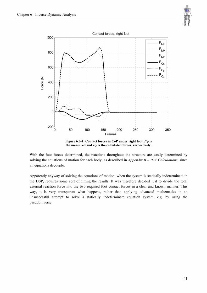
Center of Pressure The center of pressure (CoP) is the point on the ground where the resultant of the ground reaction forces is acting. This is per definition a point within the support polygon, since no force can act outside of it. When the ZMP resides within the support polygon in the SSP, the CoP and ZMP coincides for balanced walking (Sardain & Bessonet, 2004). According to (Wollherr, 2005) the CoP can be calculated easily using feedback from force-torque sensors in the feet.


18

Balanced Gait As previously mentioned the goal of this project is to produce a biped robot capable of dynamic walking, including the heel-strike and toe-off phases of gait. Wollherr (2005) distinguishes between the following types of gait balances

• Statically balanced gait: GCoM and the ZMP always reside within the support polygon. • Dynamically balanced gait: ZMP resides inside the support polygon, but GCoM leaves it.

o Balletic gait: when the support polygon is reduced to a line in e.g. the toe-off phase in SSP and the ZMP lies on that line.

• Unbalanced gait: Both ZMP and GCoM leave the support polygon. Statically balanced gait is characterized by being slow and applying short steps, whereas dynamically balanced gait is faster and can utilize longer steps. Balletic gait is presumably the most difficult to achieve, but will probably also be the most human-like kind of gait, why it is desired. Unbalanced gait can be further divided into a forward or sideways unbalance. If the robot is out of balance sideways, it will lead to overturning of the whole robot. If, on the other hand the robot is only out of balance forward, in the sense that it is rotating around the contact point of the trailing leg. This does not necessarily lead to overturning, because it can regain its balance by accepting the weight of the falling robot with the leading leg.

3.4 Summary This chapter has described some of the essential definitions of human gait, both motion descriptive, as well as balance related terms. The chapter concludes the initial analysis of the challenge of designing a biped robot. Existing robots have been investigated and the main principles of walking is now clear. Hence, a requirements specification is setup for the robot to be designed, based on the previous chapters.

Chapter 4 - Requirements Specification

19

4 Requirements Specification Through the investigation of existing robots and human walking principles, it has become clear which degrees of freedom that is the most important in order to obtain a dynamic gait, and that it is important to implement a foot capable of performing toe off. The requirements presented here have been established in collaboration with all participants of the project. The specification is subdivided into wishes and demands. These requirements will be evaluated at the end of the report.

4.1 Demands • The robot must be able to perform dynamic walking.

o Include starts and stops and standing still. o The robot must be able to make a turn. o The robot must use the heel strike, toe off method while walking.

• The robot must consist of 17 actuated DoFs, distributed as illustrated in Figure 4.2-1. • The robot must be autonomous in terms of actuators, sensors, computer and power supply. • The topology of the robot must be anthropomorphic

o Height 1800mm, higher than most existing robots. o Body parts should have human proportions.

• The budget is limited to 500.000DKK o Mainly to cover expenses of raw material and components, not workshop hours.

• The robot must be able to walk with a constant velocity of 1m/s. • It must be possible to determine the reaction forces between the ground and foot. • The robot should have a lifespan of 1000 operating hours. • The robot must include onboard power supply for 15 minutes of operation. • The mechanics of the robot must be completed before the autumn semester 2007.

4.2 Wishes • Minimize the total weight and energy consumption. • Maximize the similarity of the robot gait compared to that of humans. • The robot should distinguish itself from the existing

o Ability to sit down and rise from a chair. o Ability to climb a 0.15m high curb/obstacle.

• Ability to accumulate and release energy to reduce power consumption. • High degree of modularity in the design, for future upgrades. • Ability to imitate dysfunctional walking, however only through control.

Chapter 4 - Requirements Specification

20

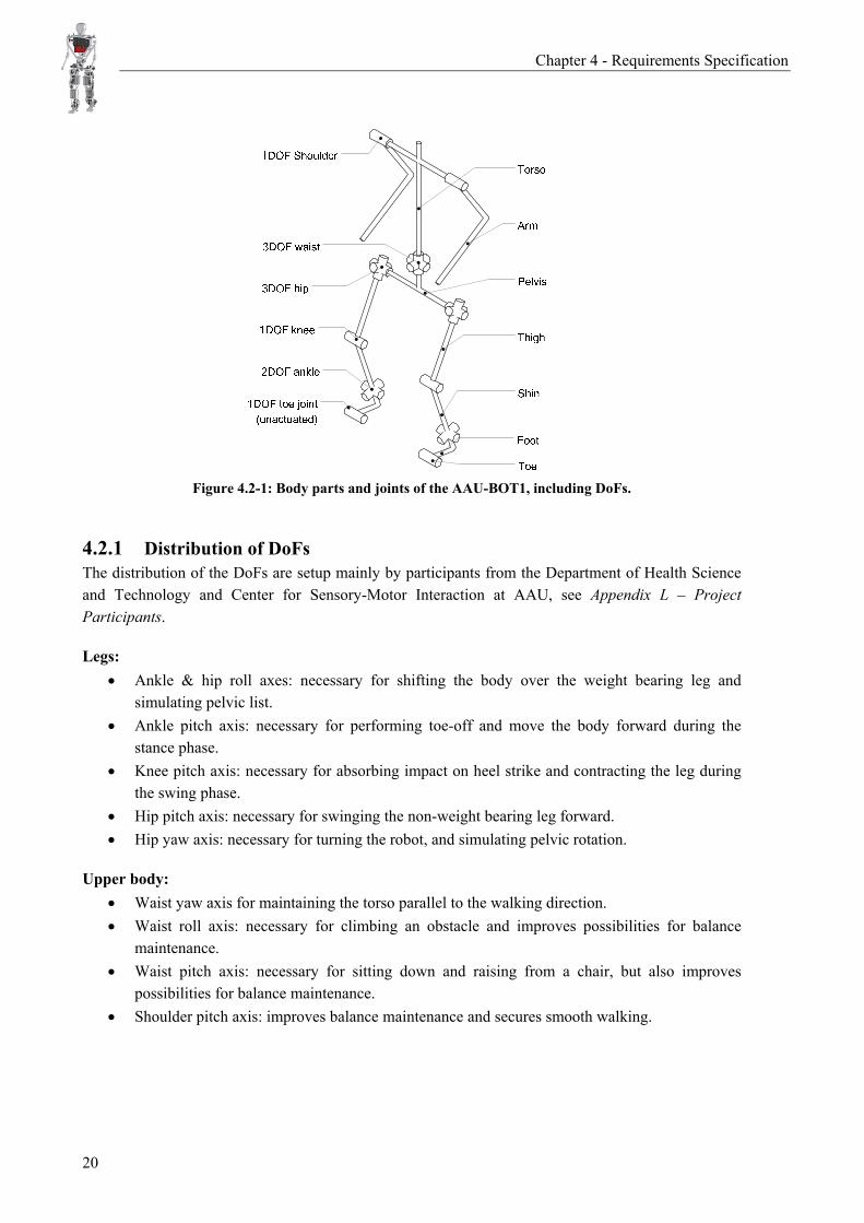
Figure 4.2-1: Body parts and joints of the AAU-BOT1, including DoFs.

4.2.1 Distribution of DoFs The distribution of the DoFs are setup mainly by participants from the Department of Health Science and Technology and Center for Sensory-Motor Interaction at AAU, see Appendix L – Project Participants.

Legs: • Ankle & hip roll axes: necessary for shifting the body over the weight bearing leg and

simulating pelvic list. • Ankle pitch axis: necessary for performing toe-off and move the body forward during the

stance phase. • Knee pitch axis: necessary for absorbing impact on heel strike and contracting the leg during

the swing phase. • Hip pitch axis: necessary for swinging the non-weight bearing leg forward. • Hip yaw axis: necessary for turning the robot, and simulating pelvic rotation.

Upper body: • Waist yaw axis for maintaining the torso parallel to the walking direction. • Waist roll axis: necessary for climbing an obstacle and improves possibilities for balance

maintenance. • Waist pitch axis: necessary for sitting down and raising from a chair, but also improves

possibilities for balance maintenance. • Shoulder pitch axis: improves balance maintenance and secures smooth walking.

Chapter 5 - Gait Experiment

21

5 Gait Experiment This chapter describes the gait experiment performed in an effort to obtain a valid and thorough description of a human gait kinematics. These data are essential in the subsequent inverse dynamics analysis, which shall determine the loads used for designing the robot. The experiment is performed in the Gait Laboratory facility of the Center for Sensory-Motor Interaction department of AAU.

5.1 Laboratory Equipment The applied laboratory equipment is investigated prior to the experiment in order to avoid potential pitfalls, and secure the best use of the equipment. The motion of a test person is recorded by a motion capture system and the ground reaction forces under the feet are measured using force platforms, both systems are connected to the same data logger, and are thus synchronized in time.

5.1.1 QTM Motion Capture The laboratory possesses a Qualisys Track Manager (QTM) system, which is a 3D motion capture system that consists of 8 cameras, arranged as illustrated in Figure 5.1-1. QTM records the positions of multiple markers attached to the body of a test person. At least three markers on each limb are necessary for calculation of both position and orientation. To clarify the markers during the experiment, the cameras are equipped with LED’s that emits infrared flashes to illuminate the markers (QTM, 2005). A suitable sampling rate of 240frames/sec is applied, the maximum for the system, which has proven sufficient in earlier experiments. The system output is the spatial coordinates of all the markers over time. The system only covers a measuring space of approximately 3m long (x), 1m wide (y) and 2m high (z), so the motion to be recorded is to be choreographed carefully.

Figure 5.1-1: Screenshot from the QTM data handling program, illustrating the camera set up and the

positioning and orientation of the global coordinate system. The green dots represent the markers and the white lines represent virtual bones.


22

5.1.2 Force Platform The force platform system is an OR6-7-1000, with a vertical load capacity up to 4450N, by Advanced Mechanical Technology Inc, based on strain gauge measurements. Two of these force platforms are installed in the Gait Laboratory for the measurement of the ground reactions under the feet of the test person. They are placed on the gait trajectory, such that the test person will step on them within the measuring space of the motion capture system. They are placed in such a way, that the test person will step on one with each foot, thereby measuring the ground reactions in both SSP and DSP. The size of a force platform is 508x464mm (AMTI, online), so it requires some timing of the gait pattern and step length, to ensure stepping on both platforms. The force platforms can measure all six components of the ground reaction, and calculate the CoP, relative to the platform coordinate system, see Figure 5.1-2. These values can easily be transformed to global by recording the position of the force platform’s local coordinate system in the motion capture system.

Figure 5.1-2: A force platform and its local coordinate system (AMTI, online).

5.2 Experiment Procedure The experiment is performed by recording the motion and ground reactions of the test person as he performs the specified load cases. In order to achieve a certain level of repeatability, the load cases must be very specific, and the experiments must be performed very similarly. A total of six experiments are performed for each load case to verify that the obtained results possesses the required repeatability. The repeatability can then be visually verified, and an average can be applied in the further analysis.

5.2.1 Positioning of Markers The principal issue of the experiment is to record the global position of the test person, and the positions of the various body parts relative to each other, with respect to time. To achieve sufficient information from the experiments, the markers have to be placed correctly. The key is to eliminate the DoFs of the human body that is not to be implemented in the robot, while simultaneously securing that the significant motion of the remaining DoFs is recorded properly.


23

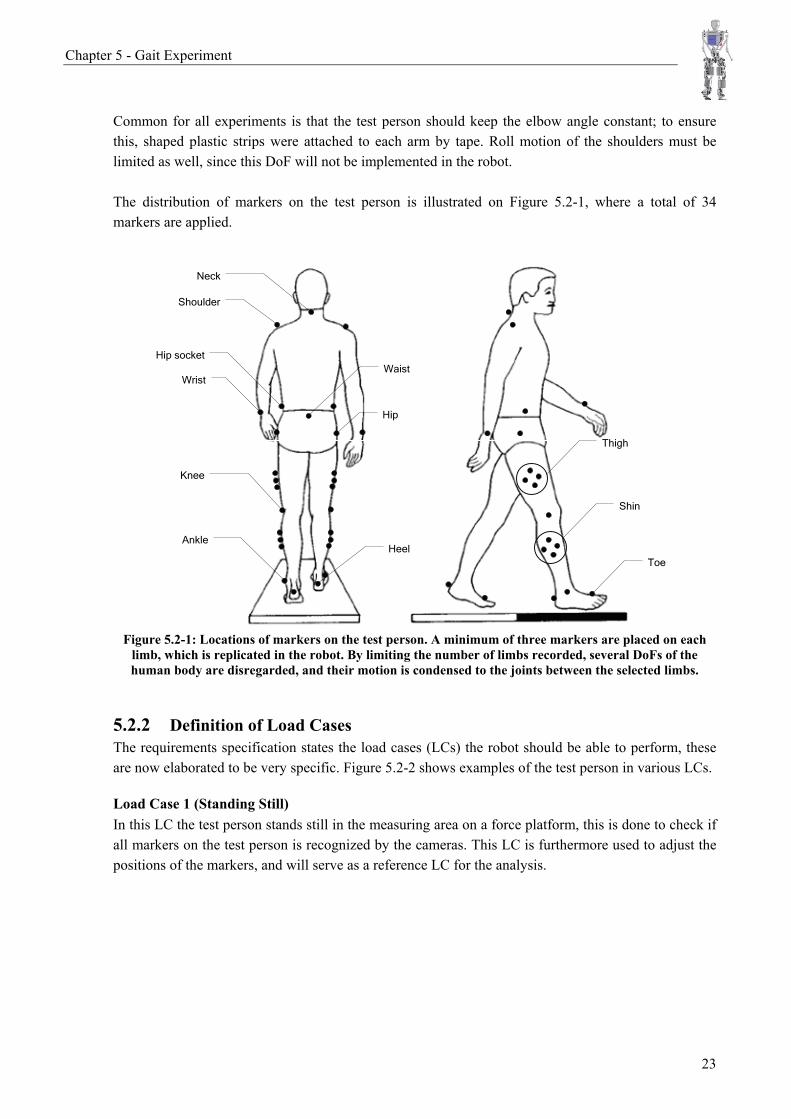
Common for all experiments is that the test person should keep the elbow angle constant; to ensure this, shaped plastic strips were attached to each arm by tape. Roll motion of the shoulders must be limited as well, since this DoF will not be implemented in the robot. The distribution of markers on the test person is illustrated on Figure 5.2-1, where a total of 34 markers are applied.

Shoulder

Neck

Hip socketWaist

Wrist

Hip

Knee

AnkleHeel

Toe

Shin

Thigh

Figure 5.2-1: Locations of markers on the test person. A minimum of three markers are placed on each

limb, which is replicated in the robot. By limiting the number of limbs recorded, several DoFs of the human body are disregarded, and their motion is condensed to the joints between the selected limbs.

5.2.2 Definition of Load Cases The requirements specification states the load cases (LCs) the robot should be able to perform, these are now elaborated to be very specific. Figure 5.2-2 shows examples of the test person in various LCs.

Load Case 1 (Standing Still) In this LC the test person stands still in the measuring area on a force platform, this is done to check if all markers on the test person is recognized by the cameras. This LC is furthermore used to adjust the positions of the markers, and will serve as a reference LC for the analysis.


24

Load Case 2 (Straight Walking) To make the experiments as similar as possible, the cycle should start with heel-strike of the right leg, and they should be performed with a uniform velocity of 1m/s. To accommodate the latter request, a treadmill was applied to adjust the walking velocity of the test person and using a metronome, the step frequency was maintained stable. The test person starts walking outside the measuring space of the motion capture system, achieving a stable constant velocity of 1m/s before entering the measuring space. While the test person walks along the specified path, he is to step on the two force platforms, marking the start of the recorded cycle with the heel-strike of the right leg on the first force platform. This LC, together with LC 6 and 7, is considered the most important, because it is of top priority that the biped should be able to walk straight, including starting and stopping. This LC is probably the most demanding regarding the joint velocities.

Load Case 3 (Sitting Down) LC 3 starts with the test person standing straight up with both feet positioned on a force platform and his arms hanging relaxed along his torso. Thereafter, the test person sits down on a chair with a steady operation without making use of his arms for support.

Load Case 4 (Raise From Seat) LC 4 is the exact opposite situation of LC 3. LC 4 starts when the test person is sitting straight up on a chair, with both feet positioned on a force platform and his arms hanging relaxed along his torso. The next phase in LC 4 is for the test person to rise from the seat, without using his arms to push off, which is analogue to the way the robot will raise from a chair. Thereafter the test person shall stand in straight posture with his arms hanging along his torso. This LC, together with LC 3 and 5, will probably be the most demanding, regarding the knee and hip joint torques. Together with LC 3 this LC will give information about the most extreme movements that will occur in the knee, hip and waist joints.

Load Case 5 (Curb Climbing) In LC 5 the test person stands in front of a 0,15m high obstacle, positioned on a force platform, with his right foot positioned on the other force platform. The test person will raise his left leg, and step on to the obstacle. The test person stands still on the obstacle for approximately 3 seconds, where after he steps down backwards.

Load Case 6 (Start Walking) In LC 6 the measurement starts when the test person is in standing position in front of a force platform, the test person starts with his right leg and steps forward on to the force platform, the test person continues walking throughout the measuring area, approaching a velocity of 1m/s. Several experiments are performed to record the ground reactions under both feet.


25

Load Case 7 (Stop Walking) In LC 7 the test person starts walking outside the measuring area with a velocity of 1m/s, when the test person enters the measuring area, he slows down and stops. Like the previous LC, several experiments are performed to record the ground reactions under both feet.

Figure 5.2-2: The test person with markers attached to the body. Load cases; straight walking (left), curb climbing (middle) and sitting on / raising from chair (right).

5.2.3 Experiment Evaluation The results from the gait experiment are the trajectories of the markers attached to the test person. Figure 5.2-3 shows an example of one such trajectory, i.e. the trajectory of the marker attached to the waist/pelvis.

0 0.2 0.4 0.6 0.8 1

0

0.5

1Recorded pelvis trajectory

x [m

]

0 0.2 0.4 0.6 0.8 10.35

0.4

0.45

y [m

]

0 0.2 0.4 0.6 0.8 11.02

1.04

1.06

z [m

]

time [s]

Figure 5.2-3: Example of the results from the gait experiment; the recorded pelvis trajectory during the straight walking load case.


26

During and after the execution of the experiment several issues of uncertainty presented themselves. Firstly, the markers attached to the test person were attached to his skin or clothes, with the consequence that they could move relative to the bones. A similar effect is present in the foot/ankle, since the skeleton is not particularly rigid in this area. Therefore, the three markers that define e.g. the foot can move relative to each other, without the foot moving, which will be perceived as motion by the system, even though the skeleton is stationary. Secondly, the floor in the Gait Laboratory, being very soft and with the markers attached relatively loosely to the skeleton, and due to the relative slow sample rate, the effects of impact on heel-strike is not observable in the recording. The computational treatment of the results data also inflicts on the precision. During recording recurring glitches is present in the marker trajectories, e.g. due to markers being hidden by body parts. These are repaired manually by spline interpolation, and data loss should be minimal. However, the results are also quite scattered, and it was necessary to apply some smoothing in order to obtain nice two times differentiable curves.

5.3 Summary This chapter has described the conducted gait experiment in terms of equipment and approach. Since none of the above mentioned issues can be improved upon by available means, the results are regarded as the best available. The task is now to determine the joint loads associated with the recorded motion. This is done using inverse dynamics, as described in the next chapter.

Chapter 6 - Inverse Dynamic Analysis

27

6 Inverse Dynamic Analysis This chapter describes the development of a parametric program/model for the inverse dynamic analysis (IDA) of a human or humanoid robot. Initially the analysis is carried out for a human, but the parametric nature of the program allows for easy replacement of inertial and geometric specifications for the subject analyzed. Using input generated by motion capture described in the previous chapter, the purpose of the analysis is to determine the forces and moments present in the joints of the given multibody structure. These loads are of great importance for the design of the robot, and will serve as a basis for the dimensioning of this. The procedure applied for the analysis is to use motion capture data as input for a kinematic analysis which will provide input for a kinetic analysis which in turn will provide the forces and moments responsible for the analyzed motion. The chapter is widely based on (Nikravesh, 1988), (Damsgaard, 2001), (Wollherr, 2005) and (Hansen, 2006).

6.1 Definitions and Assumptions In order to perform this kind of inverse dynamic analysis it is necessary to idealize the problem a great deal. The major assumption taken, is that the motion of the test person, measured using motion capture, is based on many more DoFs and bodies than considered for the robot. The movement of the different bodies (body segments) of the test person therefore has to be condensed to the 17DoFs and 10 bodies of the robot. Furthermore, the exact geometric and inertial properties of the body segments of test person are unknown and very difficult to determine, why estimates from (Vaughan et al., 1999) have been applied in the analysis. The estimates are listed in Table 6.1-1.

Body Mass [kg] Mass moment of inertia [kg*m2] Torso, head 35.5 Iξξ=1.962 Iηη=1.771 Iζζ=0.052 Pelvis 7.9 Iξξ=0.091 Iηη=0.032 Iζζ=0.096 Arms 5.8 Iξξ=0.151 Iηη=0.171 Iζζ=0.034 Thighs 6.8 Iξξ=0.087 Iηη=0.086 Iζζ=0.021 Shins 3.6 Iξξ=0.053 Iηη=0.052 Iζζ=0.005 Feet 1.1 Iξξ=0.001 Iηη=0.007 Iζζ=0.006

Table 6.1-1: Estimates of inertial properties around the body’s CoM. The bodies that constitute the robot in the analysis are considered completely rigid, i.e. no deformation is considered, which definitely, is not the case for human body segments. This assumption allows for splitting up the motion of the bodies in to linear and angular motion of the CoMs of the bodies, since all particles making up the bodies cannot move relative to each other. This assumption is justified by the fact that the motion due to deformations of the bodies is negligible compared to the over-all motion of the bodies.


28

6.1.1 Notation In the following i refers to the body number, and nb denotes total number of bodies, in this analysis nb=10. All vector quantities are defined positive in the directions of the positive global coordinate system axes. Vectors are denoted bold underlined letters: e.g. s, matrices are similar, but with a double underlining e.g. A, scalars use standard italic typography e.g. k.

Skew Matrix The skew matrix is a tool used to ease vector multiplication, i.e. taking the cross-product of two vectors. (Nikravesh, 1988) defines the skew matrix a for an arbitrary three-dimensional vector a as

follows

00

0

x z y

y z x

z y x

a a aa a aa a a

⎡ ⎤−⎡ ⎤⎢ ⎥⎢ ⎥= ⇒ = −⎢ ⎥⎢ ⎥⎢ ⎥⎢ ⎥ −⎣ ⎦ ⎣ ⎦

a a (6.1)

The skew matrix is used instead of the cross-product

× =a b ab (6.2)

The name obviously refers to the fact that the matrix is skew symmetric. The use of the skew matrix allows for the application of a wider range of manipulations (matrix-vector operations) to a given expression.

6.2 Kinematic Analysis The purpose of the kinematic analysis is to determine both the translational and angular accelerations and other kinematic quantities to provide for the kinetic analysis. Furthermore the angular velocities determined in this analysis are used in the selection of actuators. The kinematic analysis of an open chain system comprising position, velocity and acceleration analysis, of both translatory and rotary motion, can be divided into the following steps according to (Hansen, 2002).

• Determine number of bodies and apply local coordinate system to each. • Determine the transformation matrix associated with each body. • Determine the position of each local coordinate system in local coordinates. • Determine the same in global coordinates. • Determine the relative (angular) velocity and acceleration of each joint. • Determine angular velocity of each body. • Determine angular acceleration of each body. • Determine the velocity of each body. • Determine the acceleration of each body.

This approach has been applied in the analysis, although not strictly in this sequence.


29

Open vs. Closed Chain Systems In this analysis the robot is regarded as an open chain system. The ground connection(s) are modeled as applied forces at variable positions under the feet. This way, the robot is considered as a floating open chain, with the waist joint as a floating base. Open chain systems are characterized by being easily handled analytically, since every body can be completely described relative to the previous body in the chain. Closed chain systems, on the other hand, often result in nonlinear equations of such complexity, that they cannot be handled analytically. Closed chain systems therefore often have to be analyzed using iterative equation solvers, e.g. Newton Raphson solvers.

Kinematic Determinacy A system is said to be kinematically determined if it comprises as many drivers as DoFs, as it is the case in this IDA. In this case, the kinematic analysis can be performed independently from and prior to the kinetic analysis, which eases the process greatly. The equations of motion (EoMs) will only have the reaction forces as unknowns in the kinetic analysis, which results in a system of linear equations that is easily solved. If fewer drivers than DoFs are present, the system is kinematically indeterminate. This means that the kinematic and kinetic problems are coupled and must be solved simultaneously, which often results in a combination of differential and algebraic equations that must be solved numerically.

6.2.1 Position and Orientation Analysis The notation regarding position analysis used, is presented in Figure 6.2-1. The global coordinates system xyz serves as main reference, whereas the local body-fixed ξηζ serves as a tool in the analysis, since several parameters are easier expressed locally than globally, e.g. geometry and inertial properties. Each body is assigned a body number i, the global vector ri describes the position of the ith body’s CoM in global coordinates. The local coordinate systems are all positioned in the CoM of the bodies. All local terms are denoted with an prime, e.g. s’j/i, which is the vector from the CoM of the ith body to the joint connecting the ith body to the jth, expressed in local i-coordinates. The s vectors describe the position of either joints between bodies or other points of interest for the analysis, e.g. ground contact points.

iη

iξiζ jη

jξjζ

body i

body j

x

y

z

irjr

/j is/i j

sP

Figure 6.2-1: Coordinate systems and vector notation.


30

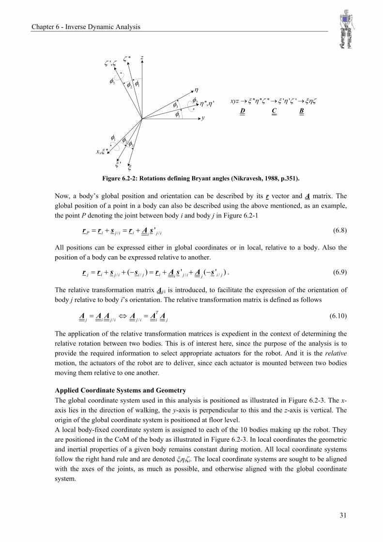
In order to completely define the global position of an arbitrary point, e.g. P, one must also describe the orientation of the local coordinate systems relative to the global. This furthermore provides the ability to transform quantities between local and global coordinates and vice versa. In this analysis, Bryant angles are chosen for the description of the angular orientation of the local coordinate systems and thus the bodies. Bryant angles describe the angular orientation of a given coordinate system relative to another, by three consecutive rotations around the system axes. The sequence of rotations is fixed to rotation about the '' 'x η ζ− − axes respectively, see Figure 6.2-2. The orientation of a body i can be described by its transformation matrix, either relative to the main reference or relative to another body j, using the Bryant angles. These transformation matrices are denoted Ai and Aj/i respectively. These matrices are formed by the direction cosines (or unit vectors) of the new axes that follow the three rotations, as explained in the following. As illustrated in Figure 6.2-2 the rotations 1 2,φ φ and 3φ transforms the initial xyz coordinate system

into the resulting ξηζ coordinate system. The temporary transformations due to a single rotation can be described by the partial transformation matrices

2 3 3

1 1 3 3

1 1 2

1 0 0 0 00 0 1 0 00 0 0 0 1

c s c sc s s cs c s c

φ φ φ φφ φ φ φφ φ φ φ

−⎡ ⎤ ⎡ ⎤ ⎡ ⎤⎢ ⎥ ⎢ ⎥ ⎢ ⎥= − = =⎢ ⎥ ⎢ ⎥ ⎢ ⎥⎢ ⎥ ⎢ ⎥ ⎢ ⎥−⎣ ⎦ ⎣ ⎦ ⎣ ⎦

2

2

D C B (6.3)

The total transformation is described by the matrix A

2 3 2 3 2

1 3 1 2 3 1 3 1 2 3 1 2

1 3 1 2 3 1 3 1 2 3 1 2

c c c s sc s s s c c c s s s s cs s c s c s c c s s c c

φ φ φ φ φφ φ φ φ φ φ φ φ φ φ φ φφ φ φ φ φ φ φ φ φ φ φ φ

−⎡ ⎤⎢ ⎥= = + − −⎢ ⎥⎢ ⎥− +⎣ ⎦

A DC B (6.4)

Where c and s denotes cosine and sine, respectively. A is orthogonal, which means that its transpose is its inverse (Kreyszig, 1999, p.381)

1 T− =A A (6.5)

This property is widely used. The transformation is carried out by matrix-vector multiplication, as an example, the local vector s’ is transformed to global coordinates in eq. (6.6) and back in eq. (6.7).

'=s As (6.6)

' T=s A s (6.7)


31

z''ζ',ζ ζ

y

'', 'η η

η

, ''x ξ

'ξ ξ

1φ2φ3φ

1φ 2φ3φ

1φ

2φ3φ

'' '' '' ' ' 'xyz ξ η ζ ξ η ζ ξηζ→ → →D C B

Figure 6.2-2: Rotations defining Bryant angles (Nikravesh, 1988, p.351).

Now, a body’s global position and orientation can be described by its r vector and A matrix. The global position of a point in a body can also be described using the above mentioned, as an example, the point P denoting the joint between body i and body j in Figure 6.2-1

/ /'P i ij i j ii= + = +r r s r A s (6.8)

All positions can be expressed either in global coordinates or in local, relative to a body. Also the position of a body can be expressed relative to another.

/ / / /( ) ' ( ' )j i ij i i j j i i ji j= + + − = + + −r r s s r A s A s . (6.9)

The relative transformation matrix Aj/i is introduced, to facilitate the expression of the orientation of body j relative to body i’s orientation. The relative transformation matrix is defined as follows

/ /T

j i j i j i i j= ⇔ =A A A A A A (6.10)

The application of the relative transformation matrices is expedient in the context of determining the relative rotation between two bodies. This is of interest here, since the purpose of the analysis is to provide the required information to select appropriate actuators for the robot. And it is the relative motion, the actuators of the robot are to deliver, since each actuator is mounted between two bodies moving them relative to one another.

Applied Coordinate Systems and Geometry The global coordinate system used in this analysis is positioned as illustrated in Figure 6.2-3. The x-axis lies in the direction of walking, the y-axis is perpendicular to this and the z-axis is vertical. The origin of the global coordinate system is positioned at floor level. A local body-fixed coordinate system is assigned to each of the 10 bodies making up the robot. They are positioned in the CoM of the body as illustrated in Figure 6.2-3. In local coordinates the geometric and inertial properties of a given body remains constant during motion. All local coordinate systems follow the right hand rule and are denoted ξiηiζi. The local coordinate systems are sought to be aligned with the axes of the joints, as much as possible, and otherwise aligned with the global coordinate system.


32

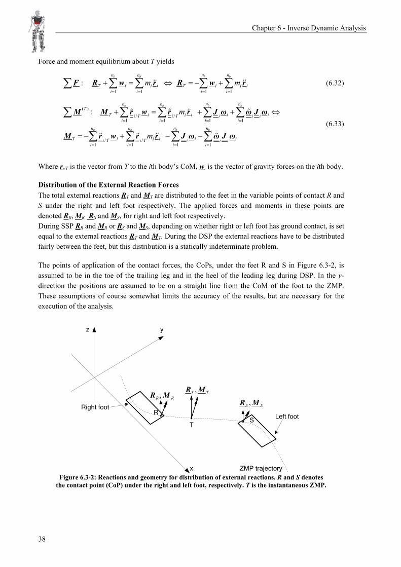
Furthermore, the local coordinate systems are defined in such way, that they lock out oblivious DoFs, i.e. the DoFs comprised by a human body, but not by the robot. This is done by defining them dependent on each other, e.g. axes of coordinates systems on different bodies are defined as being perpendicular or parallel. In Figure 6.2-3, the body numbers are denoted in squares, the joints are denoted by a letter. R, S and T are the points defining the ground contact, R is the variable point under the right foot, where the external reaction force acts on the robot, S is the corresponding point for the left foot. T is the point where the total external reaction is calculated, which will be elaborated on later.

1ξ 1

η

1ζ

Figure 6.2-3: Body and joint numbering, position

and orientation of global and local coordinate systems. The axes of coordinate system 1 are shown

in the top-left for exemplification.

R

S

s 4/1

s3/1

s2/1

s1/4

s8/10

sS/10

sR/9

s7/9

s 1/2

s 1/3

s5/4s6/4s 4

/5

s 7/5

s 4/6

s 8/6

s5/7

s9/7

s6/8

s10/8

Figure 6.2-4: Vectors from CoMs to joints,

defining the geometry applied in the analysis.

Local Coordinate System Orientation The unit vectors ξi, ηi and ζi define the axes of the local coordinate systems. They are set up based on the marker positions described in Chapter 5 Gait Experiment. The trajectories of markers include the points denoted A-K, in Figure 6.2-3. These of course varies through time as the marker positions vary, therefore new axes have to be calculated for each time-step in the input. The unit vectors describing the orientation of coordinate system 1 is shown in Figure 6.2-3, these are determined as follows. A support point L is defined in the middle between points B and C in Figure 6.2-3, with the position


33

( )12L B C= +r r r (6.11)

Using L and known marker positions, the unit vectors describing orientation of body 1, can be defined

1C B

C B

−=

−r rηr r

, 1

L A

L A

−=

−r rζr r

and 1 11=ξ η ζ . (6.12)

Based on these vectors one can setup the transformation matrix for body 1 as.

1 11 1⎡ ⎤= ⎣ ⎦A ξ η ζ . (6.13)

The transformation matrices for the remaining bodies are set up using the same approach, see Appendix B – IDA Calculations, for details.

Body Positions The position and orientation of all bodies are determined using transformation matrices and the geometry vectors established in Figure 6.2-4. In the lack of a constant ground connection or base, the waist joint (A in Figure 6.2-4) is used as such, and the measured trajectory is applied to describe its motion. The structure is thus analyzed as an open chain with a floating base. The base position r0 is given by

0 A=r r (measured waist point trajectory). (6.14)

The position of body 1 (the torso) is then given as

1 0 4 /11( )= + −r r A s . (6.15)

The position of body 2 (right arm) is

2 1 2 /1 1/ 21 2( ) ( )= + + −r r A s A s (6.16)

And so forth. This way all bodies’ position and orientation are described by their r-vector and A-matrix respectively.

6.2.2 Relative Motion The relative motion between bodies is important because it defines the range, in which the mechanical counterpart to the human body segments and the actuators need to be able to operate.

Relative Rotations

The relative rotations (Bryant angles 1 2 3/[ ]T

j iφ φ φ φ= ) are extracted from the relative

transformation matrices as described by (Nikravesh, 1988, p.352)

2 13

231

2

123

2

sin

sincos

sincos

aa

a

φ

φφ

φφ

=−

=

−=

22 2

331

2

113

2

cos 1 sin

coscos

coscos

a

a

φ φ

φφ

φφ

= ± −

=

=

(6.17)


34

Where akl is the components of the relative transformation matrix Aj/i. The angles are obtained by the inverse tangent as follows

1 sintancos

ii

i

φφφ

− ⎛ ⎞= ⎜ ⎟

⎝ ⎠ (6.18)

In the program, atan2 is used since it is singularity-free, and yields the angle in the correct quadrant. As it is seen from eq. (6.17) there is a singularity for 22 nπφ π= + , where n is an integer.

Relative Angular Velocity The relative angular velocity ωj/i of body j relative to body i, in global coordinates is obtained by

( )/ /j i j i

ω φ=ω T (6.19)

And in local coordinates of body i

( )/ /

' 'j i j iω φ=ω T (6.20)

Where /j i

φ is the time derivative of the relative rotations, and T(ω) is a coefficient matrix given by

1 3 3( ) ( )( )

2 3 3

2

cos cos sin 0cos sin cos 0 , '

sin 0 1

Ti

ω ωω

φ φ φφ φ φφ

⎡ ⎤⎢ ⎥= − =⎢ ⎥⎢ ⎥⎣ ⎦

T T A T (6.21)

It is seen that the angular velocity is dependent on both the relative rotations and their time derivatives, through the T(ω) matrix. The angular acceleration on the other hand is straightforwardly determined by time differentiation of the angular velocity. In the analysis, both the relative angular velocity and acceleration are calculated in local coordinates, since these values are sufficient for the analysis.

6.2.3 Velocity Analysis The velocity and angular velocity of all bodies are determined by the following equations, using the open chain approach, thus referring both quantities to previous body in the chain.

/ /'j i j i i j ii= + = +ω ω ω ω A ω (6.22)

The angular velocity of the first body (the torso) is calculated in relation to the global reference frame, which has zero angular velocity and acceleration. The velocity of the jth body’s CoM is obtained by differentiation of eq. (6.9), and is given by

/ /' ( ' )j i j i i ji ji j= + + −r r ω A s ω A s (6.23)

since i ii=A ω A . Actually eq. (6.23) is a result of the use of the product differentiation rule, but since

both local s vectors are constant in their respective local coordinates, they have zero time derivatives.


35

6.2.4 Acceleration Analysis By differentiation of eq. (6.22), the angular acceleration of a body is given as

/ /' 'j i j i j ii ii= + +ω ω A ω ω A ω (6.24)

The acceleration of the jth body’s CoM is likewise obtained by differentiation of eq. (6.23).

/ / / /' ' ( ' ) ( ' )j i j i j i i j i ji i j ji i i j j j= + + + − + −r r ω A s ω ω A s ω A s ω ω A s (6.25)

Thus all kinematic quantities are determined, and the objective of the kinematic analysis is fulfilled. These quantities are now used in the kinetic analysis.

6.3 Kinetic Analysis The purpose of the kinetic analysis is to determine the forces and moments that entail the observed motion. These are to be applied as a basis for the dimensioning of the mechanical parts of the robot and in the selection of suitable actuators. The foundation of the kinetic analysis is the equations of motion or equilibrium equations, i.e. Newton’s second law of linear motion and Euler’s equation of rotational motion. These equations establish a relationship between the motion and the forces and moments that result in this motion. By solving these equations for every time-step a complete overview, of the distribution of the unknown forces and moments throughout the structure, are obtained, since the motion is already completely determined.

6.3.1 Newton-Euler Equations of Motion The very familiar equation of linear motion is defined as follows. The application of this equation demands that the reference coordinate system is an inertial frame, i.e. a frame that does not accelerate. The chosen global coordinate system applied in this analysis is assumed to be an inertial frame, since it is positioned stationary on the floor.

iiim=∑F r (6.26)

This equation states that the sum of forces acting on the ith body equals the mass times the acceleration of the CoM of the same body. To ease the analysis, the equation is modified to separate the gravity forces acting on a body, such that

ii iim m= −∑F r g (6.27)

Where g is a vector containing the acceleration term due to gravity. Using (6.27) the sum of forces only counts reaction forces in the joints and/or contact points. Euler’s equation of rotational motion is most conveniently expressed about the CoM of a body as follows

i i ii i i= +∑M J ω ω J ω (6.28)


36

This way both gravity and linear acceleration associated terms vanishes. If expressed about other points, the forces originating from gravity and acceleration will act in a lever arm, and thus contribute to the equilibrium of moments. The right hand side in eq. (6.28) is known as the rate of change of angular momentum, the first term is the rotational equivalent of the right hand side in eq. (6.26) and the last term includes moments due to centripetal, centrifugal and Coriolis forces. The equations of motion are setup for all bodies using Free Body Diagrams (FBD) and Kinetic Diagrams (KD). These can be found in Appendix B – IDA Calculations. The equations can be set up both in local and global coordinates, here the global expressions are chosen.

6.3.2 Inertial Properties The right hand side of the equations of motion consists of kinematic terms and inertial terms. These inertial terms are the mass mi and the inertia matrix Ji, which are associated with linear and angular motion, respectively. The inertia matrix contains the mass moments of inertia for the ith body around all applicable axes. It is defined as

' ' 'V

dm= −∫J s s (6.29)

Which is, the integral over the volume V of a body, where the vector s’ describes the position of the mass element dm, in a local centroidal body fixed coordinate system. It is most conveniently expressed in local coordinates, since the moments of inertia are constant here regardless of the orientation of the body.

'i i i i i i

i i i i i i

i i i i i i

i

I I I

I I I

I I I

ξ ξ ξ η ξ ζ

η ξ ηη η ζ

ζ ξ ζ η ζ ζ

⎡ ⎤⎢ ⎥

= ⎢ ⎥⎢ ⎥⎢ ⎥⎣ ⎦

J (6.30)

Where the diagonal terms indicate the mass moments of inertia around the local coordinate system axes, the off-diagonal terms are the products of inertia, which are only present for non-symmetric structures. Since the equations of motion are computed in global coordinates, the inertia matrix also has to be transformed to global coordinates.

Transformation of the Inertia Matrix The moments of inertia applied in the analysis are extracted from CAD models, because of the relative advanced geometry applied. Analytical calculation of the moments of inertia could be very interesting in other contexts, e.g. in optimization tasks or other contexts where explicit formulation and inherent easy altering is an advantage. In such case it is expedient to setup the inertia matrix for subsystems of simple geometries, e.g. cylinders or cubes.


37

Transformation of J’ by the rotation A yields a new inertia matrix, J.

' T=J A J A (6.31)

By applying (6.31), a local inertia matrix is easily transformed to global coordinates. Now the right hand sides of the equations of motion are accounted for. The left hand side is merely a summation of reaction and contact forces and moments.

6.3.3 Solving the Equations of Motion In order to solve the systems of equations of motion, setup in Appendix B – IDA Calculations, it is necessary to divide the analysis in two cases; SSP and DSP. During the SSP, the entire external reaction force must be applied to the foot in the CoP, which coincides with ZMP in SSP. The system of equations is easily solved by starting in the extremities and calculating all reactions for each body towards the waist joint. During the DSP the distribution of reactions between the two feet becomes statically indeterminate, and it is only possible to determine the sum of the reactions.

Determination of External Reactions

TT

1

bn

iii

m=∑ r

1

bn

iii=∑J ω

1

bn

ii ii=∑ω J ω

1

n

ii=∑w

TRTM

RS

/1

bn

iii Ti

m=∑r r

Figure 6.3-1: FBD and KD for the entire robot, T is positioned in the ZMP.

The total external reactions caused by the interaction between the robot and the environment are denoted RT and MT. These are calculated in the ZMP (point T), why MT only has a vertical component. By calculating the external reactions here, one avoids the distribution of eventual horizontal reaction moments between the feet. The position of the ZMP is pre-calculated by kinematic values only.


38

Force and moment equilibrium about T yields

1 1 1 1:

b b b bn n n n

T i T ii ii ii i i i

m m= = = =

+ = ⇔ = − +∑ ∑ ∑ ∑ ∑F R w r R w r (6.32)

( )/ /

1 1 1 1

/ /1 1 1 1

:b b b b

b b b b

n n n nT

T ii i iii T i T i i ii i i i

n n n n

T ii i iii T i T i i ii i i i

m

m

= = = =

= = = =

+ = + + ⇔

= − + − −

∑ ∑ ∑ ∑ ∑

∑ ∑ ∑ ∑

M M r w r r J ω ω J ω

M r w r r J ω ω J ω (6.33)

Where ri/T is the vector from T to the ith body’s CoM, wi is the vector of gravity forces on the ith body.

Distribution of the External Reaction Forces The total external reactions RT and MT are distributed to the feet in the variable points of contact R and S under the right and left foot respectively. The applied forces and moments in these points are denoted RR, MR, RS and MS, for right and left foot respectively. During SSP RR and MR or RS and MS, depending on whether right or left foot has ground contact, is set equal to the external reactions RT and MT. During the DSP the external reactions have to be distributed fairly between the feet, but this distribution is a statically indeterminate problem. The points of application of the contact forces, the CoPs, under the feet R and S in Figure 6.3-2, is assumed to be in the toe of the trailing leg and in the heel of the leading leg during DSP. In the y-direction the positions are assumed to be on a straight line from the CoM of the foot to the ZMP. These assumptions of course somewhat limits the accuracy of the results, but are necessary for the execution of the analysis.

T

ZMP trajectoryx

z y

RS

,T TR M,R RR M

,S SR M

Left footRight foot

Figure 6.3-2: Reactions and geometry for distribution of external reactions. R and S denotes

the contact point (CoP) under the right and left foot, respectively. T is the instantaneous ZMP.


39

To handle this problem of indeterminacy several approaches were considered. They are discussed briefly below.

1. Distributing the sum of reactions using a spline distribution, see Figure 6.3-3, to achieve a smooth transition of weight bearing from trailing to leading leg, assuming the point of contact under the feet to be approximated as being stationary during DSP. This approach was tested, however it does not satisfy equilibrium in the structure, since the assumed magnitude and position of the applied forces does not match the real distribution completely.

2. Employing a FEM beam model, but this would require estimates of the stiffnesses of the structure. This approach was not tested, since it would be quite time demanding, both in setting up and carrying out, because a new analysis would have to be set up and conducted for every time-step.

3. Solving the system of equations using the pseudoinverse, this resembles finding the least squares solution to a system with indefinitely many solutions. This approach was tested, but the resulting distribution was un-natural and therefore not satisfactory.

The first approach was chosen since, it seems to yield the most promising results. As seen in Appendix B – IDA Calculations the reactions on the bodies are calculated from the extremities and towards the waist joint connecting the torso and pelvis (A in Figure 6.2-3). Using this approach it is possible to verify whether equilibrium is maintained in the structure, by comparing the reactions in joint A. These reactions must be identical if equilibrium is to be maintained. On the other hand, if the reactions deviates, it is an indication that the forces applied to the feet differs from the actual foot forces experienced during the gait experiment. This is because the reactions in point A, when calculated from the feet up, are determined by the applied foot forces. Whereas the reactions in point A, when calculated from above down through the torso, are determined by the motion of the test person in the gait experiment. The contact (foot) forces are a highly dependent on the geometric and inertial properties as well as the motion of the test person / robot. Since only the motion are measured and geometric and inertial properties are estimates, which not only affect the contact forces, but also the motion (due to deviations in geometry), it is very difficult to determine an exact set of contact forces. Not even the measured contact forces from the gait experiment can be regarded as exact for this analysis, since the analysis is based on estimated geometry and inertia. Therefore, inaccuracies are to be expected. The total external reactions RT and MT are distributed to the feet in the variable points of contact R and S under the right and left foot respectively, in the following way.

R TR

S TL

ff

= ⋅= ⋅

R RR R

(6.34)

fR and fL are distribution factors, that together equals one. The value of e.g. fR – the factor that scales the reactions acting on the right foot – is determined by whether the right leg currently is the leading or trailing and time, i.e. the progression through the DSP as illustrated on Figure 6.3-3.


40

::

:R lead

R trail

leading f fRight leg

trailing f f=⎧

⎨ =⎩ (6.35)

::

:L lead

L trail

leading f fLeft leg

trailing f f=⎧

⎨ =⎩ (6.36)

The moment MT is distributed similarly, but is of less interest since it only has a small component around the vertical axis.

leadf1

[ ]time s0

trailf

.duration of DSP

Figure 6.3-3: Factors for distributing the total external reactions between the feet during the DSP,

determined by fitting at cubic spline. ftrail is associated with the trailing leg and flead with the leading. The entire weight of the robot shifts from the trailing leg to the leading leg during the DSP.

The reactions obtained by application of this distribution agree quite well with the reactions measured during the gait experiment, discussed in Chapter 5 Gait Experiment, as seen in Figure 6.3-4. Furthermore, by applying this distribution the calculation of the foot reactions becomes completely independent of the inertial properties of the test person, for whom the measured distribution applies. However, after dividing the total external reaction forces in to two, RR and RS respectively, they need be moved from the ZMP to a point under the feet, where they act. This leads to some uncertainty regarding the results of the analysis, but visual inspection of the results show that the error is insignificant in the sense that it doesn’t affect the maximum joint torques. These naturally occur during the SSP, where the entire weight of the robot is applied to one leg, and this phase of the walking cycle is not affected by this problem.


41

0 50 100 150 200 250 300 350-200

0

200

400

600

800

1000

Frames

Forc

e [N

]

Contact forces, right foot

FMxFMy

FMz

FCx

FCyFCz

Figure 6.3-4: Contact forces in CoP under right foot, FM is the measured and FC is the calculated forces, respectively.

With the foot forces determined, the reactions throughout the structure are easily determined by solving the equations of motion for each body, as described in Appendix B – IDA Calculations, since all equations decouple. Apparently anyway of solving the equations of motion, when the system is statically indeterminate in the DSP, requires some sort of fitting the results. It was therefore decided just to divide the total external reaction force into the two required foot contact forces in a clear and known manner. This way, it is very transparent what happens, rather than applying advanced mathematics in an unsuccessful attempt to solve a statically indeterminate equation system, e.g. by using the pseudoinverse.


42

6.4 Inverse Dynamics Program Because of the immense amount of bookkeeping required, the IDA described in the previous was carried out in a program, see Appendix PQ – Inverse Dynamics Program. This program is briefly described here, and the routine is illustrated in Figure 6.4-1.

Read associated input:Define load case

Align and take average

Get contact states Set gait phases

Correct trajectories

Data structures

Visualize results

/j iA

/' j iφ

/' j iφ /' j iω

/' j iω

iω

iω

ir

ir

ir

iA

( )' ωT

Forceplate data ..x zF

Marker trajectories ..A Kr

Inertial properties , 'i im J

Geometry specs. / /' , 'i j j is s

Geometry specs. / /' , 'i j j is s

Marker trajectories ..A Kr

Joint associated

Body associated

Inertial properties , 'i im J

Kinematics , , ,i i i ir r ω ω

Setup local CS’s i i iξ η ζ

ZMPr TRContact state

Gait phase

iJ

Body orientation iA Geometry specs. / /,i j j is s Reactions ,R MSetup & solve:

iii

i ii i i i

m=

= +

∑∑

F r

M J ω ω J ω

Contact forces ,R SR R

Figure 6.4-1: Schematic representation of inverse dynamics program.

Initialization The program is initiated by defining which load case to investigate, this determines which set of marker trajectories and forceplate data is read from files. Furthermore, the geometry and inertial properties of the structure (human/robot) to be analyzed are read from files. These data are parametrically defined, such that they can easily be replaced, and an analysis of a different design can be performed. Several data structures are initiated to facilitate the bookkeeping and ease the transfer of data internally in the program and externally for the handling of the results. These data structures contain all relevant information sorted under joint, body and general associations.


43

The input from the gait experiment, i.e. marker trajectories and forceplate data, is read for 5 data sets and aligned in time, then an average data set is extracted. The marker positions are corrected to match joint positions in the human body, i.e. shifted inwards in the body to the center of e.g. the hip socket. Based on the forceplate data, information regarding the feet’s contact state throughout the analysis is setup to assist the later kinetic analysis, also information describing the different gait phases is setup. All data that varies through time is stored for each time-step, which in this analysis equals each frame shot by the cameras of the motion capture equipment. A sample rate of 240Hz was applied, which for a normal walking cycle of approximately 1.2sec yields a total number of 288 frames / time-steps.

Kinematic analysis Local body fixed coordinate systems are setup based on the marker trajectories, which, together with the defined local geometry specifications, form the foundation of the entire kinematic analysis. As illustrated in Figure 6.4-1, all kinematic quantities are determined from these and their variation through time.

Kinetic analysis The kinetic analysis uses the kinematic results as input, together with the geometry and inertial properties and the predetermined contact / gait phase information. Firstly the inertia matrix is transformed to global coordinates based on the current body orientation. This and the kinematic results are then used in the calculation of the ZMP trajectory. Then the external reactions are calculated in the ZMP and distributed to the feet according to the current contact state (SSP or DSP) and gait phase (feet orientation, e.g. toe-off position). The point of application of the (foot) contact forces are determined from the gait phase information and the discussed assumptions. The equations of motion are then setup and solved for the joint reactions, which are the only unknowns. The equation system is linear and completely decoupled and therefore easily solved.

Visualization of results All results are stored in files for easy handling and later visualization. These files are then read by the graphical user interface (GUI) called AAU-BOT Animator. A screenshot from this GUI is illustrated in Figure 6.4-2. The main purpose of the GUI is to present the results in an easy-to-understand manner and assist in the design process. This is handled by implementing an animation of the robot next to the graph showing user selected results, the graph contains a vertical line synchronized with the animation, that illustrates the instantaneous results. The GUI comprises the following features; switching between load cases, selecting animation view -3D or projected, setting time-step/frame number by slider or simply playing the animation from start. Additional visualization options include plotting of; CoM, GCoM & ZMP trajectories, global & local coordinate systems, external and foot reaction vectors. Also vectors illustrating joint reaction forces and moments and body accelerations can be shown in the animation for all or selected bodies / joints.


44

Figure 6.4-2: Graphical user interface for visualization of results from the IDA. The user selects the desired set of results from the IDA in the section Monitor parameters, here the following results are available for plotting

• Body associated: o CoM position. o CoM velocity. o CoM acceleration. o Inertial & gravity forces. o Moments from inertia. o Angular velocity. o Angular acceleration.

• Joint associated: o Relative rotation. o Relative angular velocity. o Relative angular acceleration. o Reaction forces. o Reaction moments. o Position.

Conclusively, when visualizing the joint moment- and body acceleration vectors, the animation gives a clear view to the smartness of the human body. It becomes evident how the human body e.g. lessens the knee moments by accelerating the upper body, and how the overall CoM is shifted to maintain balance. Many such observations can be made using this GUI.


45

6.5 Results from the IDA Program The results are easiest obtained from the GUI mentioned in the previous section. This section only covers a small portion of the results (straight walking load case), meant for exemplification and verification. Already published results from inverse dynamic analyses of adult humans are presented as basis for comparison. The joint reaction forces are all correct, they can easily be verified based on simple hand calculations. The joint torques, on the other hand, deserve more discussion.

0 50 100 150 200 250-100

0

100

200

Hip

Mη [N

m]

AAU-BOTReference

0 50 100 150 200 250-50

0

50

100

Kne

e Mη [N

m]

AAU-BOTReference

0 50 100 150 200 250-200

-100

0

100

Frames

Ank

le M

η [N

m]

AAU-BOTReference

Figure 6.5-1: Selected kinetic results from the IDA. The bold line shows calculated joint torques and the

thin hatched lines represent same values adapted from (Inman et al., 1981, p.86). As it is seen from Figure 6.5-1, the calculated joint torques agree quite well with published reference values. The reference values are from (Inman et al., 1981, p.86) and represent joint torques in the right legs, for four adult male test subjects walking at 1,4m/s, almost similar to the test person in the gait experiment. No reference data was found for the remaining joints; the waist, and shoulders. The human waist cannot be considered as a single biological joint, like e.g. a knee, since the flexibility of the waist originate in the spine. The results obtained for the shoulder joints are considered fairly reliable, since they only depend on the motion of the arms. The results for the waist, on the other hand is probably the most uncertain, see Figure 6.5-2. There are several issues causing this, firstly, since the waist is the final joint in the chains of bodies, the reactions calculated here must equilibrate the entire robot. The lower part is applied forces in the feet, based on harsh estimates and the only place the error in these foot forces can be remedied is in the waist. Thus, one must expect the calculated waist reactions to deviate somewhat from the correct values.


46

0 50 100 150 200 250-100

-50

0

50

100

Nm

Waist moments

Frames

Mξ,e

Mη,e

Mζ,e

Mξ,k

Mη,k

Mζ,k

Figure 6.5-2: Calculated waist moments, those with subscript k are calculated based on the kinematics of the upper body, subscript e are calculated to equilibrate the reactions from the legs. The full vertical lines

separate the SSP and DSP. From Figure 6.5-2 it is seen that especially Mη varies greatly in the vicinity of the DSP. Just before entering the DSP it is evident from animation that the robot is out of balance, since the ZMP leaves the support polygon. This is a consequence of the estimates (geometric and inertial) made in the analysis that leads to the motion not matching the analyzed structure (robot/human). The motion recorded in the gait experiment will most likely not render a different person in balance, other than the test person, because the inertia is distributed differently. Although there are some problems regarding the waist moments, the results are considered sufficient for the design of the robot. To be conservative, the waist moments of the largest magnitude is applied in the design, see Figure 6.5-2. This way, the robot will have some power reserve in the waist, applicable for recapturing balance if subjected to some unknown disturbances.

6.6 Summary This chapter has provided a complete description of the IDA, in terms of theory applied and approach used. The results cover both kinematic and kinetic quantities necessary for designing the robot, which are all available on the enclosed CD-ROM. The coming chapter describes how these quantities are applied in the dimensioning process.

Chapter 7 - Designing AAU-BOT1

47

7 Designing AAU-BOT1 This chapter presents an overview of the design phase, both in terms of the loading spectrum applied and the design approach used. Initially an appropriate loading spectrum is set up, which will lead to an appropriate overall design. Secondly, an overview of the approach used throughout the design phase is presented.

7.1 Loading Spectrum Considerations Since the mechanical structure of the AAU-BOT1 is to be designed prior to the development of the control, it is impossible to determine the exact loadings, it will be exposed to, because they will be dependent on the final control strategy. This dilemma has lead to the dimensioning approach described in the following.

7.1.1 Basis for Initial Dimensioning The most valid loading spectrum available is the one obtained from the IDA, based on the gait experiments of a test-person with roughly the same mass and geometry as the final robot design. However, this loading spectrum lacks the inclusion of effects from:

• Loads due to impact on heel-strike. • Loads due to the actual control strategy. • Loads required for balancing different inertia distribution.

To remedy these shortcomings, it is chosen to use the before mentioned loading spectrum, but scaled with a factor of 1.8. This is used both in the selection of power transmission components and the initial dimensioning of the structural components, and should lead to a suitable overall design of the robot. It is decided not to iterate over the loading spectrum using slightly altered inertia/geometry as the design takes shape, since it will still be quite uncertain, and might loose some of the validity associated with it. This is a primary concern, since the kinematics and kinetics of the analysis is highly related. If altering the inertia distribution and thus the kinetics, it is unlikely that the kinematics associated with the former inertia distribution is sufficient for balance maintenance of the new inertia distribution.

7.1.2 Loading Spectrum The selection of power transmission and initial structural dimensioning uses the loads from the inverse dynamic analysis, with the test-person inertia and multiplied by a factor of 1.8, see Appendix H - Loading Spectrum. Only the results from the straight walking load case is applied for dimensioning, since the loads obtained from the remaining load cases is regarded as being too control dependent. That is, if the motion of e.g. sitting down is not performed i perfect balance; it requires very large joint torques.


48

However, static joint torques are calculated for the robot in several extreme poses, e.g. with knees bend 90° or torso bend 45° forwards, see Appendix M – Extreme Static Joint Torques. The robot must be adequate for these static loads, and if so, it should be possible to implement the remaining load cases using intelligent control.

Straight walking Static Joint Moment axis / force direction 1.8·Max force

[N] 1.8·Maxt torque[Nm]

Max torque [Nm]

Roll / x 140 70 46 Pitch / y 158 224 107 Ankle Yaw / z 1535 45 Roll / x 119 153 Pitch / y 144 119 121 Knee Yaw / z 1467 45 Roll / x 147 244 100 Pitch / y 121 207 78 Hip Yaw / z 1346 48 - Roll / x 146 63 42 Pitch / y 83 108 115 Waist Yaw / z 961 27 - Roll / x 40 7 Pitch / y 23 9 - Shoulder Yaw / z 118 2

Table 7.1-1: Magnitude of extreme joint torques and forces, both static and from the straight walking LC, including the factor of 1.8. Actuated axes are marked with gray. Values are given in the coordinate system

of the previous body in the chain, originating in the pelvis. As evident from Table 7.1-1, the straight walking load case clearly exceeds the static loads. It is therefore only necessary to consider this load case in the dimensioning of the robot. It would be too extensive to display all plots of different aspects of the loading spectrum here, since there are several both kinetic and kinematic values for each joint/body, and all of them can be regarded in different coordinate systems depending on the purpose of their use. These data can be obtained by applying the visualization tools for the IDA, available on the enclosed CD-ROM. The required angular range of the joints can, as well as the loads, be extracted from the IDA; these are listed in Table 7.1-2. The movement range of the joints is determined based on all load cases. Not surprisingly, the knee requires the widest range for operation, primarily due to the sitting on and raising from a chair LCs.


49

Joint Axis Range Span

roll -10° 15° 25°Ankle

pitch -19° 19° 38°Knee pitch 1° 95° 94°

roll -17° 11° 28°pitch -81° 11° 92°Hip yaw -19° 27° 46°roll -13° 11° 24°pitch -56° 1° 57°Waist yaw -19° 28° 47°

Shoulder pitch -33° 6° 39°Table 7.1-2: Required angular range of joints, (Bryant angles).

The angles listed in Table 7.1-2, are regarded as minimum values. Where possible, some additional movable range is therefore preferable, also since this would allow different types of walking patterns, e.g. longer steps.

7.1.3 Basis for Verification It is chosen to leave the optimization of the system performance to be performed in the control strategy. This way, the performance of the selected power transmission can be maximized by intelligent use of different joints. Since the power transmission components comes in incremental sizes, some joints will have excess power and some will have minimum power, relative to the reference gait. This can be exploited in the final control strategy, by sparing the joints having only minimum power and using the ones with excess power intensively. To implement this, the structural parts should be dimensioned after the maximum torque of the selected power transmission components, making these the limiting factor in the design, thus enabling them to be fully exploited. The verification of the design should therefore be approached differently from the initial dimensioning, not looking at what is required, but what can be achieved. This should eliminate potential bottlenecks and maximize performance. The verification is therefore to be based on the final inertia distribution and inherent loads, without any scaling factors. It should then determine the level of excess power available, if any, in each joint such that this can be utilized when designing the final control strategy.


50

7.2 Design Approach The design phase has of course proceeded somewhat iteratively, however, the following sequence describes the overall approach.

• Selecting appropriate power transmission components i.e. motors, gears and belt drives. • Developing a mechanical design that accommodates the selected components. • Verification of the structural adequacy of the mechanical design. • Verification of power transmission components, i.e. setting appropriate restrictions which will

lead to the required life span of the robot. The necessary power transmission components are selected based on the scaled up loading spectrum described in the previous section. These account for approx. half the total weight of the robot. It is therefore necessary to select these before the mechanical structure can be designed, since the dimensions of this will be very dependent on the chosen power transmission components. The mechanical design is developed and verified in parallel using hand calculations and FEM analysis. Subsequently, when the geometry and inertia of all structural parts, and the gear and motor specifications are determined, it is possible to verify the selected gears and motors. The approach used here, is to set appropriate restrictions for the individual joint, for use in the development of the final control strategy. These restrictions shall secure the required lifespan of the robot. The remainder of the report treats the following subjects, which further verifies the design, enables contact feedback for control and suggests improvements applicable in future robots.

• Simulation of the final robot, verifying the design and components in time domain. • Development of a force/torque sensor to obtain feedback for the final control • Development of a structural optimization scheme for weight minimization.

By building a simulation environment and implementing a preliminary limited control strategy, it is possible to verify whether the composition of the mechanical design and power transmission is adequate, including all dynamic effects. This simulation is very detailed, modeling the rotating parts in the power transmission and the contact between the feet and floor, thus including the so far unknown elements affecting the loading spectrum. A six axis force/torque sensor is then developed in order to achieve a feedback signal describing the contact forces between the feet and floor, for use in the final control of the robot. This sensor is developed as a prototype and subsequently improved through experiments. Lastly, a structural optimization scheme is developed, which can be used for weight minimization of all structural components in the robot. The scheme is applied to one component for verification, but is more directed towards use in future robots, possible based on the current robot.

Chapter 8 - Power Transmission Selection

51

8 Power Transmission Selection This chapter presents the selection of the power transmission for the robot i.e. motors, gears and belt drives. A high power-to-weight ratio is necessary to minimize the overall weight. The components are selected based on the loading spectrum described in the previous chapter. This chapter is mainly based on (Maxon, 2006) and (HDG, 2006). The power transmission components for the robot is the most expensive, both financially and in their contribution to the overall weight. In order to obtain a fast dynamic walking robot, it is essential to keep the overall weight at an absolute minimum. However, selection of power transmission components, if based on manufacturer specifications, will often lead a conservative choice with inherent long operation life. The required life span of the robot is only 1000h, it is therefore necessary to review the suggested methods in order to achieve lighter, but less durable power transmission components. Furthermore, stock items are preferred, due toe the limited budget and time frame.

8.1 Motor Selection It was decided to use Maxon DC motors, since these come with excellent documentation, high performance and are used in several other biped robots, e.g. Johnnie. The Johnnie group describes how they encountered a performance limit for DC motors at 150W, if more powerful motors are required, the power-to-weight-ratio will be reduced (Gienger et al., 2000). The Johnnie group solved the problem by applying two DC motors to actuate one joint, if more than 150W is needed. DC motors have the advantage that they are easy to control, because the motor speed is proportional to the input voltage, and the torque is proportional to the current. The DC motors comes with either permanent magnet stator or a stator with field windings. Maxon DC motors are made with a wound field stator and a permanent magnet rotor, which according to (Maxon, 2006) is up to 90% more efficient than other systems. Maxon presents a stock program for each DC motor type with different properties for these stators. Brushes of e.g. graphite or metal are often used to transmit current to the rotor. The advantages of using DC motors with brushes are; low cost and easy control, only requiring a variable-resistor. On the other hand, motors with brushes can create sparks, and when the brushes press against the commutator, they create a friction force, reducing performance. DC motors can also be brushless, but then an electronic speed controller is then required for operation, making them more expensive. However, a brushless DC motor is more efficient than one with brushes, since it is not affected by the friction force from brushes. Maxon Company offers two series of DC motors that are feasibly for the robot; the RE- and the EC-series – with and without brushes, respectively. The RE-series with brushes are grouped in graphite- and metal brushes. Graphite brushes are typically used in motors with high current loads, start/stop- and reverse operations. Metal brushes are typically used in motors with small current loads and continuous operation. The motors relevant for the robot are therefore with graphite brushes. Both can


52

be delivered with encoders for position feedback. The RE series with brushes was chosen, based on experience from earlier projects at Aalborg University considering control of small DC motors, because of the inherent easier control (Rasmussen, verbal).

8.1.1 DC Motor Characteristics The characteristics of a DC motor are illustrated in a diagram that describes the linear torque / speed relationship. For constant voltage, a line describing the mechanical behavior of a DC motor can be drawn between two points; no load speed and stall torque, see Figure 8.1-1. The no load speed and stall torque is based on the nominal voltage.

Figure 8.1-1: DC motor diagram. The area under the torque-speed line is the workspace for nominal

voltage. The grey area is the continuous operation zone, in which overheating is prevented. If the voltage is lowered, a line parallel to the torque-speed line shifts to a lower value and vice versa. The behavior of the DC motor will then follow the new line made by decreasing the voltage. The motor can operate at any point under the torque-speed line, but it should be kept in mind, that the windings can be damaged if the motor overheats. To ensure that the temperature doesn’t exceed the thermal limit, it is important to limit the area under the torque-speed line to a zone for continuous operation. This zone is defined by two limits; max permissible speed and max continuous torque. Operation points within these limits will not produce wear on the commutation system and are not critical for the winding temperature. Speeds higher than the no load speed is possible, but increases electro-erosion, and shortens the service life of 20.000 hours significantly.

8.1.2 Loading Spectrum Maxon offers a calculation method for selection of suitable motors, given the loading spectrum. In this method, the working cycle for the DC motor is split up in operation points and plotted in a torque/speed workspace. There can be several points of operation, i.e. at acceleration, breaking or sudden operation stops. The operation points of maximum torque, -speed and -power will be considered here. A program is developed for the selection of feasible motors for each joint and plotting of the operation curve in the torque/speed workspace, see Appendix R – Motor & Gear Selection Program.


53

The loading specter is given by the joint moments from the inverse dynamics analysis, where the local components of the actuated axes determine the required torque to be produced by the selected motor and gear combination, see Table 7.1-1, these are determined as follows

jointaxisT

axisM = e M (8.1)

Where Maxis is the torque requried for driving a given axis, eaxis is a unit vector in global coordinates describing the axis of rotation roll/pitch/yaw and Mjoint is the determined joint moment, also in global coordinates.

8.1.3 Selection of DC Motors To identify feasible DC motors for the joints, the selection can be split up in two. One is based on continuous loads and another on momentary peak loads. Table 8.1-1 lists the final range of motors, which is selected from.

Motor Stall torqueMH [Nm]

Nom. TorqueMnom [Nm]

No load speed n0 [rpm]

Mass [g]

RE 60W 1.020 0.0882 8490 238 RE 90W 0.967 0.0965 7270 340 RE 150W 2.500 0.1840 7580 480 2x RE 150W 5.000 0.3680 7580 960

Table 8.1-1: The final range of motors to be selected from. The joint torque and velocity are calculated with respect to the motor shaft. This means that it is necessary to take the gear ratio and efficiency into consideration, when determining the requirements for the motor. The required torque to be delivered by a motor can be calculated as.

,axis,max

m max

MM

u η=

⋅ (8.2)

Where Mm,max is the maximum required motor torque, Maxis,max is the max occurring joint torque around the given axis, u is the total gear-ratio, including belt drive, and η is the efficiency of the gear. Eq. (8.2) is valid when the motor torque and velocity is in the same direction. Otherwise, if the torque and velocity is in opposite directions, the motor will act as a generator, and the gear efficiency will move to the numerator in the fraction of eq. (8.2). The required brake-torque will thereby be reduced by the gear efficiency. The required motor speed nm is traditionally given in rpm, and calculated as

60[ ] [ ]2

sminrad

sm axis,max radrev

n rpm uωπ

= ⋅ ⋅ (8.3)

Where the max angular velocity ωaxis,max is transformed to rpm. The two values, eqs. (8.2) and (8.3), are checked in the DC motor workspace, thus determining whether the values are under the torque-speed line, see Figure 8.1-1.


54

Momentary Peak Loads It should be noted that the stall torque for a DC motor is a theoretical value, and the magnets in the motor can be damaged if it should deliver this torque. The Danish distributor of Maxon motors, COMPOWER A/S, informs that the maximum allowed torque for Maxon RE motors is approximately four times the nominal torque, if only loaded for a short time (Gregersen, verbal). Thus the maximum motor torque must be obey the following limit.

4m,max nomM M< (8.4)

Continuous Loads For continuous operation, the motor workspace is restricted further by the limit of maximum continuous torque, i.e. the nominal torque. If crossing the limit of nominal torque the motor gradually heat up and within a certain time operation failure due to overheating will occur. To determine whether the DC motor overheats or not, the root-mean-square (RMS) value of the torque-time cycle can be held against the nominal torque value, provided by the manufacturer. The RMS value is a statistical measure of the magnitude of the varying torque applied, since the torque both has negative and positive signs in the work cycle, and the ordinary mean value therefore is not descriptive of the average torque delivered

21, 0

T

m RMS mTM M (t) dt= ∫ (8.5)

Where T is the cycle time and Mm(t) is the time-varying motor torque over a cycle.

Motor Overloading The DC motor can be overloaded with torques higher than the nominal torque, but only for a limited time, due to heating. This allowed overloading of the motor depends on the duration of the subsequent cooling period available. The work cycle of one step, for most of the motors, can be split up in two phases; a working phase and a resting phase, see Figure 8.1-2. These arise from the walking pattern where the legs alternately are in stance and swing phases. It can be shown that most motors in the legs have these characteristic working cycles, see Appendix F – Workspace Plots for DC Motors.


55

0 0.2 0.4 0.6 0.8 1 1.2 1.4-0.5

0

0.5

1

Time [s]

Torq

ue [N

m]

Motor Torque

Pitch Torque

0 0.2 0.4 0.6 0.8 1 1.2 1.4-0.5

0

0.5

1

Time [s]

Torq

ue [N

m]

Motor Torque

Pitch Torque

Figure 8.1-2: Examples of motor torques during the straight walking cycle;

right hip pitch motor (top) and right knee pitch motor (bottom). Since the motor only peaks a fraction of the cycle, the limit of maximum peak can be set as four times the nominal torque. An estimate of the allowed duration of maximum peak torque is based on an exponentially decreasing function, shown in Figure 8.1-3.

Figure 8.1-3: Allowed overloading of a motor as a function of

the percentage of time it is turned on (Maxon, 2006, p.36). Here T is the duration of one repeated load cycle, tON is the loaded phase and tOFF is the resting phase, the primary axis describes the percentage of the cycle in which the motor is turned on. The secondary axis describes the ratio of allowed overloading. It should be noted that the current is proportional to the torque, and thereby the value of nominal torque can be used instead. As seen, four times nominal torque is only allowed approximately 8% of the working cycle. The duration of torque peak varies in the range of 5% to 15% of the cycle time depending on the joint. Since the selections of the motors are based on the inertia of the test-person, the limit four times nominal torque will be used as a guideline. In Chapter 11, the selected DC motors will be checked for overheating with respect to the straight walking LC.


56

Motor Acceleration To verify that the selected motors can deliver the required acceleration, an equivalent mass moment of inertia is to be determined. This consists of the inertia of all the rotating parts i.e. the rotor, the belt drive, the gear unit and the driven body parts. This inertia is important to take into consideration, since choosing a larger DC motor also means that the inertia of the rotor increases, and a larger torque is thereby needed to maintain the same acceleration. The equivalent mass moment of inertia can be found by (Hansen, Note 1)

( )22 2G

m

P G Jeq R P

B B B G

J J JJ J Ju u u u

= + + + ++

(8.6)

J is the mass moment of inertia, the indices; R is the rotor, Pm is the pulley on the motor shaft, PG is the pulley on the gear input shaft, G is rotating part of the gear. JJ is the equivalent inertia of the driven bodies. uB is the gearing ratio of the belt drive, and uG is the ratio of the gear unit. The mass moment of inertia of the driven bodies is calculated as

JJ

J

MJα

= (8.7)

Where MJ is the joint torque and αJ is the acceleration of the joint. The maximum deliverable angular acceleration of the motor can then be expressed as

Hmax

eq

MJ

α = (8.8)

Which is the stall torque divided by the equivalent mass moment of inertia. This value must be larger than the required acceleration of a given joint.

Criteria used in Selecting Feasible Motors The following criteria is used in the selection, however, it proved necessary to make comprises for a few motors, since it would otherwise require more than two motors in some joints. This will be further discussed in Chapter 11Verification of Power Transmission.

,

0

4m,max nom

m RMS nom

m,max max

m

M MM M

n nα α

<

<

<

<

(8.9)

Furthermore, the motor trajectory must under no circumstance exceed the torque-speed line, since this would lead to saturation.


57

8.1.4 Motor Selection Program The selection of motors and gears is combined in a program, since they are dependent, see Appendix R – Motor & Gear Selection Program. The main criterion for a motor/gear combination, other than delivering the right torque and speed, is low weight. Figure 8.1-4 shows a flow chart of the structure of the program for the selection of feasible motor/gear combinations. The program treats one axis at the time.

Start

Check limits for DC motor (5)

Check limits for CPU-S units (10)

Calculate efficiency of gear

units (9)

Motors that respects limits is

set to 1. (7)

Gear units that respects limits is

set to 1. (11)

Motor and gear combination that

respects the limits(12)

Calculate weight of combinations

(13)

Plot the lightest combination (14)

Gear selection

Get torque and speed from IDA

(3)

Input:Joint, axis &

belt drive ratio (1)

Transform load data to local axis

(4)

DC motor data library (6)

HDG CPU-S unit datalibrary (8)

Pulley datalibrary (2)

Figure 8.1-4: Flow chart of the motor and gear selection. The gear selection will be described later.

Structure of the Motor Selection Program To limit the amount of motor/gear combinations, only roughly suitable motors and gears are considered. Therefore, 4 different motors and 5 different gears each with 5 different ratios are chosen for further consideration. Selection of a feasible motor/gear combination is based on a discrete choice, so in order to handle all possible combinations, a 3D binary array is build that is used to keep track on whether a combination is adequate or not. The array is arranged as gear size x gear ratio x motor size. Then, if a combination respects a set up limit, its associated position in the array is given the value 1 and if not the value 0. Thus, after checking all limits, all combinations of motors and gears in the array with the value one will be adequate, and the lightest can be extracted. The structure of the program is explained in the following.


58

1. The joint and axis is entered, for which a motor and gear combination is sought. The size of pulleys in the belt drive, if any, is also entered. The size of the pulleys are chosen manually, since some of these are limited by the space available at the joint.

2. The data of the chosen pulleys are added. The data contains; weight, inertia and radius of the selected pulley.

3. The results from the IDA are loaded. 4. The kinetic and kinematics from the IDA are transformed to the local coordinates of the body

where the DC motor should be mounted. 5. The restriction for the DC motor is set, and the efficiencies of all gear units are calculated. 6. Data from the DC motor library is loaded. The number of DC motors are limited to four types

of DC motors; a 60W, 90W, 150W and 2x150W. 7. All motors/gear combinations are checked against the limits set at (5). The array of

combinations is updated with 1 and 0, as described. 8-11. See gear selection in Section 8.2 Gear Selection. 12. The result from the motor selection is multiplied elementwise with the results from the gear

selection. To update the combination array to include only adequate gears and motors. 13. The weight of the DC motor, gear unit and the belt drive is calculated for each feasible

combination and the lightest is chosen. 14. Several plots are made, describing the joint workspace including limits, for evaluation.

This approach yields the selection of the following DC motors, see Table 8.1-2, where the calculated max. torque / speed and nominal torque / speed is shown as well. The robot is symmetric in the sagittal plane, why the most heavily loaded side is used in the selection of motors for both sides.

Requirements Selected Joint, axis Type

Peak motor torque [Nm]

Max speed [rpm]

4 x Nominal torque [Nm]

Nominal speed [rpm]

Waist roll 90W 0.17 2774 0.386 6490Waist pitch 150W 0.42 1585 0.744 7000Waist yaw 60W 0.15 6774 0.3528 7750Shoulder 60W 0.15 913 0.3528 7750Hip roll 2x150W 1.55 5650 1.512 7000Hip pitch 150W 0.72 6332 0.744 7000Hip yaw 60W 0.22 3033 0.3528 7750Knee pitch 2x150W 1.70 6036 1.512 7000Ankle roll 90W 0.33 2219 0.386 6490Ankle pitch 2x150W 2.02 3700 1.512 7000

Table 8.1-2: All selected DC motors are 48V. The ordering info is listed in Appendix F – Workspace Plots for DC Motors. Detailed motor specifications are available in Enclosure C – Maxon Motor Specifications.

It is assumed that two DC motors can deliver twice the torque of one motor dynamically. Since the motors are almost in standstill in the point of maximum torque, this assumption is based on a statically point of view, where two motors can deliver twice the torque of one, (Rasmussen, verbal).


59

It should be noted that the DC motors chosen for hip roll and pitch, knee pitch and ankle roll joint s have a higher RMS torque than allowed. Thus, these motors will heat up during the straight walking load case. This issue will be further addressed in Chapter 11 Verification of Power Transmission.

Motor Workspace Three plots are made for each joint, one where the motor torque is plotted with respect to the speed, another where the motor torque is plotted with respect to time and one for the gear unit. The last plot will be discussed in Section 8.2 Gear Selection. Examples of the torque-time plot is already presented in Figure 8.1-2. An example of a torque-speed plot is shown in Figure 8.1-5, for the hip and knee pitch joints, which is among the heaviest loaded.

-0.8 -0.6 -0.4 -0.2 0 0.2 0.4 0.6 0.8-1.5

-1

-0.5

0

0.5

1

1.5x 104

Torque [Nm]

Spe

ed [R

PM

]

Motor workspace. Joint No: 4 Axis: Pitch, Safety factor: 1.1

-1.5 -1 -0.5 0 0.5 1 1.5-1.5

-1

-0.5

0

0.5

1

1.5x 104

Torque [Nm]

Spe

ed [R

PM

]

Motor workspace. Joint No: 6 Axis: Pitch, Safety factor: 1.9

Figure 8.1-5: Torque-speed workspace plots for the hip pitch motor (top) and knee pitch motor (bottom). These motors are the most critical with respect to overheating, as evident from Figure 8.1-5, almost half the motor trajectory exceeds the continuous operation limit. The motor trajectory should furthermore not cross the torque-speed line, which would lead to saturation. This is not the case for any of the selected motors. The continuous operation limits can be exceeded for short periods of time, but the momentary peak torque limit should never be exceeded, since it would damage the motor. The plots of the remaining DC motors are listed in Appendix F – Workspace Plots for DC Motors. Motors for each joint are thereby selected and the basis for this selection is thoroughly discussed. The associated gears are selected simultaneously, as described in the following section.


60

8.2 Gear Selection Selecting the right gears for the motors is of major importance, since the selected DC motors operate at high speeds and low torques. For the joints of the robot, the speed-torque demand is the other way around. Suitable gears for the robot should posses the following qualities:

• High gear ratio • High efficiency • Zero backlash (or low) • Low weight

These individual points will be explained later. The volume of the gear unit should also be kept at a minimum, in order to obtain a compact humanlike design, e.g. long planetary gear heads should be avoided. The gear units should therefore have a high torque-to-volume ratio. After researching the field of existing biped robots, it was discovered that the main part of the biped robots uses Harmonic Drive gears (HDG), see Chapter 2 Existing Biped Robots. The only robot of the three investigated, that applies another gearing system is Johnnie. This is a ball screw gear system (BSG) that is implemented at the ankles joints. However, the remaining joints in Johnnie also apply HDGs. The two systems both have high efficiency and low backlash (about 1arc min.). The advantage of the HD gear system is its high gear ratios 1:50-1:160, where the BSG ratios are about 1:10-1:25 (SKF, online). An even higher output ratio is obtained by implanting a belt drive connection between the DC motor and the gear system. This way, the gear ratio can be increased, depending on the space available at the joint. Furthermore, the axes of the motors and gears can be positioned parallel instead of on the same axis.

8.2.1 Harmonic Drive Gears Harmonic Drive AG has a stock program of different ratios and gear types, for which a relative short delivery time can be expected. The company has had a close collaboration with the Johnnie group, during its production, to develop gears that fulfills the specific requirements for the robot, (Wtec, online).

Harmonic Drive Gear Design The harmonic drive gear is an assembly of three main parts; an outer ring named circular spline, a metal cup named flexspline and an elliptic steel disk named the wave generator, see Figure 8.2-2. The wave generator is used as the input and is mounted inside the flexspline, which is usually used as the output. The wave generator is mounted in the flexspline, which will deform to an elliptical shape. This assembly is inserted inside the circular spline; see Figure 8.2-1, which give two points of intersection between the circular spline and the wave generator. The flexspline has teeth machined into the outer surface of the steel cup, and the circular spline has teeth machined on the inner surface of the ring, see Figure 8.2-2. The flexspline has two teeth less than the circular spline. When turning the wave


61

generator one reversal, assuming that the circular spline is fixed, the flexspline will rotate two teeth in the opposite direction. The gear ratio of the HDG depends on whether the circular spline or the flexspline are fixed. When the circular spline is fixed, the ratio of the HDG can be calculated as

flexspline teethRatioflexspline teeth circular spline teeth

=−

(8.10)

If instead the output is on the circular spline, and the flexspline is fixed, the gear ratio will be the same plus one and in the same direction.

Figure 8.2-1: Operation of a Harmonic Drive gear. Left: the HDG in initial position; the grey arrows are opposite to each other. Middle: the wave generator is turned 90 deg clockwise. Right: the wave generator

is turned one revolution clockwise and the flexspline is rotated two teeth in opposite direction. (Powertransmission, online)

The advantage of the HDG system is that there are always up to 30% teeth engaged. In comparison, a planetary gear set has only about six teeth engaged (Powertransmission, Online). The large number of teeth provides minimum backlash, in the order of 1 arc min, whereas e.g. in a Maxon planetary Gearhead GP 81 (20-120 Nm) the backlash is from 1-2 deg (Maxon, 2006).

Figure 8.2-2: HDG component set.

(Powertransmission, Online)

Figure 8.2-3: HDG unit. This model is a CSD unit, but the configuration is similar to the applied CPU-S, that is shown to

the right. (HDG, 2006)


62

To reduce the number of parts in the robot it was decided to apply HDG units, and not component sets where housings should be designed separately for each gear. The HDG units are compact assemblies, where the three parts of the HDG system and an out- and input shaft are integrated in a gear house, see Figure 8.2-3 (right). The units are heavier than component sets, due to the bearings, shafts and house, but the advantage is that they can be mounted directly on the robot. Harmonic Drive AG offers a wide selection of HDG units for all purposes. One of these units is interesting for the robot; which are the CPU-S unit that has an input shaft, which makes implementation of a belt drive easy, see Figure 8.2-3 (right).

CPU-S Mass [kg]

Nominal torque TN [Nm]

Max repeatedpeak torque TR [Nm]

Max momentarypeak torque TM [Nm]

Max dynamic tilting moment MT [Nm]

Max input speed nin [rpm]

14 0.64 7.8 28 54 73 850017 0.95 24 54 110 114 730020 1.50 40 82 147 172 650025 2.50 67 157 304 254 560032 5.40 137 333 647 587 4800Table 8.2-1: Properties of the gears, which is selected from (ratio 1:100), see Enclosure D – CPU-S.

As described in Chapter 2 Existing Biped Robots WABIAN uses the HDG unit systems, whereas Johnnie uses the HDG component sets. The HDG component set has the advantage that the designer of the joint can decide where to reinforce the joint structure. As mentioned earlier the group that built the Johnnie robot had a close collaboration with Harmonic Drive AG and had some gears specially manufactured for them. For instance, a wave generator in aluminum, and a circular spline modified as a T-shape in order to reduce weight. This reduced the mass moment of inertia by 50% compared to a standard HDG (Pfeiffer et al., 2002). This way, a lighter and faster accelerating gear unit can be achieved.

8.2.2 Selection of HDG Units Harmonic Drive AG, offers a calculation method for gear selection. This method is based on the output torque, tilting moment and operating life. Mainly the output torque based approach will be used here. Figure 8.2-4 shows the five smallest CPU-S units plotted with respect to their weight and the limit for repeated peak torque.

Figure 8.2-4: Left: weight of CPU-S units. Right: limit for repeated peak torque (ratio 1:100).


63

As seen, the weight of the CPU-S units increases exponentially with respect to the unit size, which is also the case for the torque. However, the torque-to-weight ratio is almost constant. The maximum torque occurring during straight walking should not exceed the limit for repeated peak torque, according to the calculation method recommended from HD. A first hand calculation of the weight of all gear units, based on the above plots and maximum joint torques in Chapter 7 Designing AAU-BOT1, yields a total of 45.8kg gears. This is almost the same weight as the entire Johnnie robot, which has the same number of DoFs. The calculation method is based on the wave generator bearing life, and should lead to a service life of 35.000h, if the average input speed is 2000rpm (HDG, 2006, pp.124-153). Since the required life of the robot is only 1000h, the recommended calculation method is therefore reviewed. After some iteration in gear selection, it was decided to disregard the repeated peak torque limit and furthermore disregard the safety factor of 1.8, discussed in Chapter 7 Designing AAU-BOT1, to minimize the total mass of the gears. This approach allowed for selection of gears weighing only 18.1kg. The consequences in form of reduced fatigue life and possible degraded performance must be accepted, and will be discussed later. The CPU-S unit contains grease for lubrication of bearings and flexspline. Exceeding the allowed average torque TA will lead to heating of this grease. However, since the operation time for the robot will be in relative short separated periods of time, exceeding TA is accepted. The maximum allowed tilting moment of the gear unit should not be exceeded. This value is not based on the life of the bearings or the flexspline. This value is based on the maximum allowed deflection of the components in the gear unit, and exceeding it will damage the gear.

Criteria Used in Determining Feasible HDGs In order to avoid excessively heavy gears, the loading spectrum is only scaled up when considering the limit for the tilting moment, because, if exceeded, the gear will be damaged. Exceeding the remaining limits only shortens the expected service life of the gears.

• Avg. output torque < repeated peak torque limit TR. • Max. output torque < momentary peak torque limit TM. • Max. tilting moment (including a factor of 1.8) < tilting moment limit MT • Input speed nm < max input speed nin.

8.2.3 Efficiency of the HDG Unit The efficiency of the gear unit depends on the following values; input speed, working temperature, output torque, unit size and gear ratio. The efficiency of a lubricated CPU-S unit at rated torque can be determined by using the efficiency graph (HDG, 2006, p.152). Assuming that the ambient temperature is constant at 20°C, a linear relationship between speed and efficiency can be assumed, see Figure 8.2-5.


64

Figure 8.2-5: Left: efficiency depending on the ambient temperature and the average input speed.

Right: efficiency depending on speed at constant ambient temperature. This relationship can be established for all units, and the efficiency for the units at rated torque ηR can be determined. Since the torque vary over time, it is necessary to compensate the rated torque, by calculating a torque constant V. By using the average torque the average efficiency can be calculated

, 0.2 1.0av

N

TV VT

= ≤ ≤ (8.11)

The torque constant V is based on the average torque Tav at the output shaft and the rated-torque at rated-speed TN, this value can be found in the technical data for the HDG units. V is used to determine the correction factor K by using the V-K-graph, see Figure 8.2-6 (left), it should be noted that the value of V is between 0.2 to 1. If V exceeds this interval, it is set to the boundary value.

1.0

0.8

0.7

0.6

0.5

0.4

0.30.2

0.9

0.2 0.4 0.6 0.8 1

500rpm1000rpm2000rpm3500rpmC

orre

ctio

n fa

ctor

6 6 7 0 04 4 6 8 02 2 5 7 00 0 3 5 50 0 0 2 2

⎡ ⎤⎢ ⎥⎢ ⎥⎢ ⎥⎢ ⎥⎢ ⎥⎢ ⎥⎣ ⎦

Figure 8.2-6: Left: V-K graph for the gear unit (HDG, 2006, p.152).

Right: correction values ηe in percent for the gear units, dependent on ratio and unit size. The efficiency is to be corrected by ηe which represents the gear unit size and its ratio. The total efficiency η can then be found.

( )R eKη η η= ⋅ + (8.12)


65

For the gear selection program the V-K-graph is approximated as a log-function by taking 9 readings of the V-K-graph at the mean input speed of 1000rmp.

0.3log( ) 1K V= + (8.13)

This gives a small error in the result, but is estimated as slightly conservative. But since most of the gear units operate in the vicinity of the maximum torque limit, the correction factor K becomes one, and a relative high efficiency is achieved.

Program for Selection of HDG Units The selection of the gear units applies the same discreet method as for the DC motors, illustrated by the flow charts in Figure 8.2-7, see Appendix R – Motor & Gear Selection Program.

Check limits for CPU-S units (10)

Calc. efficiency of gear units (9)

Gear units that respects limits is

set to 1. (11)

Get torque / speed(7)

DC motor selection

HDG CPU-S units data library

(8)

Figure 8.2-7: Flow chart for the gear unit selection.

The program procedure is briefly described below

7. Torque and speed are calculated with respect to the input shaft of the gear unit. The speed of the DC motor is reduced by the belt drive ratio, and the torque is multiplied by the belt drive ratio and efficiency.

8. The specifications of five CPU-S units with five gear-ratios each are loaded. It should be noted that the CPU-S-14 and 17 don’t have five ratios, but are given five ratios. For the non-existing ratios of these units, the combinations marked as unfeasible by a 0 in the combination-array.

9. The efficiency of each gear unit and gear-ratio is calculated with respect to the load cycle. The mean efficiency of each gear unit with respect to the gear-ratio is send to the DC motor selection program.

10. The limits for speeds and torques are set. Speeds are checked at the input shaft and torques at the output shaft.

11. The gear-ratio for each gear unit is checked against the limits. The combination-array are updated simultaneously, keeping track of whether a combination is feasible (1) or not (0).

Finally, the lightest gear-ratio-motor combination that respects all limits are chosen for the robot design.


66

Selected Gear Units The following gear units are all selected using the program, except for the hip and waist yaw joints, which are discussed later.

Joint Size Ratio Required torque / avg. speed

[Nm] / [rpm]

Selected Max. torque / avg. speed

[Nm] / [rpm] Waist roll 14 100 35 395 54 3500Waist pitch 17 120 60 216 86 3500Waist yaw 17 100 15 1076 110 3500Shoulder pitch 14 100 5 431 54 3500Hip roll 20 120 135 555 147 3500Hip pitch 20 120 115 1222 147 3500Hip yaw 17 100 27 601 110 3500Knee pitch 17 100 66 1943 110 3500Ankle roll 14 100 39 224 54 3500Ankle pitch 20 160 124 1106 147 3500Table 8.2-2: The selected CPU-S gear units for the robot. The maximum torque is at the output shaft and

the average speed is at the input shaft. The maximum torque is the momentary peak torque. The yaw-axis gears in the hip and waist are the only ones that have no support on the output shaft, see Chapter 9 Mechanical Design. Therefore, these gear units are controlled for violating the limit of tilting moment. The worst case tilting moment is the vector sum of the roll and pitch peak moments occurring in the hip and waist joints. The maximum output torque values and the average input speed are listed in Table 8.2-3. The maximum allowed speed is not listed since the only motor that can deliver a speed higher than the allowed maximum input speed is the 60W DC motor if it is applied to a CPU-20-S gear, and such combination does not occur. Joint Actual

moment [Nm] Dynamic tilting moment [Nm] CPU-14-S CPU-17-S

Static tilting moment [Nm] CPU-14-S CPU-17-S

Hip 207 Waist 109

73 114 144 328

Table 8.2-3: Tilting moments of hip and waist yaw gear units. Since both the hip- and the waist joint tilting moments are larger than the allowed dynamic tilting moments of the CPU-14-S units, which are otherwise adequate, they are discarded. Instead CPU-17-S units were chosen. The waist joint tilting moment is under the dynamic limit, and the hip joints having a speed of only 4rpm at peak moment is considered as statically loaded. The selection of motors and associated gear units are now complete. It is now possible to select a suitable power supply, i.e. batter, which will be discussed in the following.


67

8.3 Selection of Batteries One of the demands for the robot is to make it autonomous, and therefore carry a battery. The nominal voltage of the battery should be 48V, required by the DC motors. The power needed for operating the robot has to be calculated, in order to determine a suitable battery.

Power Loss in DC Motors When a DC motor is subjected to an input voltage from a power supply, an electrical power Pel is applied to the motor. Since an electrical motor has internal resistance, the Pel used for running the motor can be divided in two. That is; mechanical power Pmech associated with the speed and torque, and Joule power loss PJ arising from the resistance of the windings, associated with heat.

el mech JP P P= + (8.14)

The motor input is the voltage U and current I, which produces a torque M and a velocity ω. The current makes the internal resistance Rwindings heat up, causing a power loss.

2, ,el mech J windingP U I P M P I Rω= ⋅ = ⋅ = ⋅ (8.15)

The mechanical power and the Joule power loss over a walking cycle are calculated for each DC motor, using the same program as for the motor and gear selection. Thus, the total electrical power can be estimated, and suitable batteries and servo amplifiers can be chosen. It was decided to use 48V DC motors to minimize the required current. A low current is to be preferred since the power loss is dependent on the current squared, and servo amplifiers are restricted by the current. Servo amplifiers with less current capacity can therefore be applied. As mentioned before, the drawn current of the motor is proportional to the produced torque. Therefore, the current can simply be calculated by multiplying the torque with a constant, given by the manufacturer. The trajectory of the DC motors involves all four quadrants of the workspace; see e.g. Section 0 Motor Selection. When a DC motor operates in the 1st and 3rd quadrants, it requires power, and when in 2nd and 4th quadrant, it generates power. Figure 8.3-1 shows the torque and velocity direction for each quadrant.

ω ω

ωω

Figure 8.3-1: The four quadrants of a DC motor workspace (Maxon, 2006).


68

Since the DC motors generates power when the torque and speed have different directions, it can theoretically deliver power to other motors that are using power. However, in order to be conservative in the selection of batteries, this issue is not included and the produced power is neglected. The power delivered by the battery can be split up in three parts. The mechanical power and Joule power loss, but power loss in the servo amplifiers also have to be taken into consideration. In the calculation of power used by the robot, the Joule power loss is therefore doubled to compensate for the power loss in the servo amplifier. The max efficiency of the servo amplifier is above 95%, according to (Maxon, 2006). The maximum and mean currents to be drawn from the battery are determined by summation of the currents to the individual motors over the load cycle. The power loss from each DC motor can then be found by using the calculated current in eq. (8.15). The maximum and the mean current for the battery and each DC motor are shown at Table 8.3-1. Battery capacity can easily be determined based on the calculated power, so that it can perform the straight walking cycle for 15 minutes, as specified in Chapter 4 Requirements Specification A rule of thumb says that only 2/3 of the capacity of the battery must be used, so extra capacity must be included. Since high currents are needed when starting the DC motors, a battery of Nickel Metal Hydride (Ni-MH) is used, since it can deliver a high starting current and is rechargeable.

Current Maximum [A] Mean [A] Waist roll 2.2 0.8Waist pitch 5.8 3.1Waist yaw 2.5 1.1Shoulder pitch 2.0 0.7Hip roll 9.2 1.4Hip pitch 9.6 3.3Hip yaw 4.0 1.4Knee pitch 14.1 4.5Ankle roll 5.3 1.3Ankle pitch 16.6 4.7Total, all motors 9.1

Table 8.3-1: The maximum and mean current from all DC motors. The selected battery is a Ni-MH battery with a capacity of 3,3Ah, a nominal voltage of 7,2V and a continuously discharge current of 30A. By connecting seven of these in series, a final voltage of 50,4V can be achieved. The weight of the seven assembled battery is 2,6kg. A fully charged battery has enough power for 15 minutes of walking, see Figure 8.3-2. The only drawback of this battery is that it takes up to 16 hours to recharge an empty battery, but since they are cheap and easy to replace, this is not considered a problem. Both the maximum peak and mean current required by the robot is well beneath the limits of this battery. The data sheet of the battery is found in Enclosure A – Battery Specifications.


69

Figure 8.3-2: Plot of the discharge time for one battery cell, see Enclosure A - Battery

Since the peak current of each motor is now determined, a suitable set of servo amplifiers can be selected for the local control of the motors.

8.4 Selection of Servo Amplifiers The DC motors can be controlled by a simple variable resistance, but since high performance and reliability are required, servo amplifiers (SA) from Maxon are chosen, because they are optimized for the chosen Maxon motors. They have three types of control; speed, position and current control. Since the DC motor trajectories are in all four quadrants, as mentioned above, the SAs should also be able to operate in all four quadrants. The SAs comes in two models, a standard Eurocard format and one in a module house. There is no difference in performance, but the weight of the Eurocard version for a 5A SA is only 175g, whereas the one in module housing weighs 400g. Since students should handle the robot, the SAs in module housing are chosen. The module housing SAs exist in two versions; 5A or 10A. Both allow a maximum current of twice the nominal current. The weight is the same, and the price is only 10% higher for the 10A version.

DC motor Max current DC motor[A]

Max SA current [A]

SA Model (4-Q-DC-ADS)

Number

Waist roll 2.2 10 4-Q-DC-ADS 50/5 1Waist pitch 5.8 10 4-Q-DC-ADS 50/5 1Waist yaw 2.5 10 4-Q-DC-ADS 50/5 1Shoulder pitch 2.0 10 4-Q-DC-ADS 50/5 2Hip roll 9.2 20 4-Q-DC-ADS 50/10 4Hip pitch 9.6 20 4-Q-DC-ADS 50/10 2Hip yaw 4.0 10 4-Q-DC-ADS 50/5 2Knee pitch 14.1 20 4-Q-DC-ADS 50/10 4Ankle roll 5.3 10 4-Q-DC-ADS 50/5 2Ankle pitch 16.6 20 4-Q-DC-ADS 50/10 4

Table 8.4-1: The selected servo amplifiers for the robot. The 10A version is chosen, for the motors with a maximum current close to or above 10A. The specifications and distribution of the SAs are listed in Table 8.4-1.


70

8.5 Summary This chapter has presented the approach used in the selection of suitable power transmission components. Initially, a set of limits are determined, which separates feasible motors and gears from infeasible. A selection is then made using a developed program, which determines the lightest possible combination of motor and gear for a given joint. Furthermore, a suitable battery is selected, which will provide onboard power supply for 15minutes of walking. Lastly, electronic components, i.e. servo amplifiers, are selected for local motor control. The next chapter presents the development of the physical structure of the robot, which accommodates the selected power transmission components.

Chapter 9 - Mechanical Design

71

9 Mechanical Design This chapter presents the robot design, in terms of the mechanical structure as well as integration of the power transmissions selected in the previous chapter. The mechanical structure will be described to explain some of the underlying considerations that have led to this solution. After an introductory overview of the robot, some general considerations regarding available manufacturing technologies and materials will be discussed. This is followed by an in-depth discussion of the design details, concluded by an evaluation of the overall design. The complete design is documented in the enclosed technical drawings, see Appendix XYZ – Technical Drawings.

9.1 Design Overview Figure 9.1-1 presents a CAD model of the robot, seen from the front (right) and back (left), the overall dimensions are; height 1800mm, width 660mm and depth 270mm. The total mass is approximately 70kg, assuming 2kgs of bolts, screws and wiring. The 17 actuated joints are driven by 23 DC motors, which each require their own servo amplifier. The mechanical power transmission for all joints is composed by a HD gear unit connected to the motors by a belt drive. Detailed images of the final design, is available in Appendix O – Design Overview.

9.1.1 Weight Distribution The main objective in the design of the robot is to keep the weight on a minimum. As illustrated in Table 9.1-1, the structural/load carrying components, only accounts for less than a third of the total mass of the robot. The remaining covers other necessary components, such as power transmission, electronics and minor construction elements.

Item Mass [kg] Share [%] Electronics, wiring (est.) 4.0 5.7Motors, encoders 9.9 14.1Servo amplifiers 10.0 14.3Belt drives, tightening, mounting 2.5 3.6Gears 18.1 25.8Batteries 2.6 3.7Bearings, bolts, screws (est.) 2.0 2.9Non-structural components, total 49.1 70.1Structural components 20.9 29.9Total 70.0 100

Table 9.1-1: Distribution of weight by component type.


72

Figure 9.1-1: Overview of the design of the AAU-BOT1, front (right) and back (left).

9.2 Design Considerations The key to a successful robot design is low weight, since reducing weight starts a positive circle, reducing the demanded joint torques and thereby the requirements on both motors and gears, which again can reduce the weight of the structural components. Lower weight will also ensure low power consumption and reduce stresses in the load carrying structure, prolonging its life. Low weight is sought by removing as much material as possible from areas with low stress levels, and exploiting the necessary components, e.g. gears and servo amplifier housing, in the load carrying structure. This way, very little material is needed around a gear or under a servo amplifier box.


73

To obtain an efficient and durable power transmission, the rotation axes of gears, axles, bearings and motors must be sufficiently aligned, both angular and translational. Each HD gear unit contains two bearings, which is exploited in one side of every joint, together with 3rd bearing in the opposite side of most joints. But when adding an output axle and a third bearing to the gears any misalignment will shorten the life of the gear. This is to be compensated for by two measures. Applying plain spherical bearings allows for angular misalignment. Mounting the third bearing axially floating in an in-plane adjustable plate allows for elimination of possible translational misalignment. Due to the quite limited time available for construction of a structure this complicated, the design process is based on simple calculations and estimates for many parts. The more critical parts are analyzed using FEM (CosmosWorks), but many parts are designed by intuition. The results from the IDA are applied as the loading spectrum in the design phase, although multiplied by 1.8 as discussed in Chapter 7 Designing AAU-BOT1.

9.2.1 Manufacturing Technologies The robot is manufactured in the workshop associated with the Institute of Mechanical Engineering. Due to the ongoing development of the robot it was decided, in collaboration with the workshop staff, that they should manufacture all parts. This would not only keep the manufacturing costs at a minimum, and last minute design changes could easily be implemented, contrary to what might be expected if manufactured outside the University. This choice limits the design freedom to what is possible to manufacture in the workshop. Fortunately, the workshop possesses a number of advanced manufacturing machines, including a 5 axis milling / turning center, a CNC lathe and an electrical-discharge wire cutting (EWC) machine. Since both budget and time is limited, effort is put into designing simple parts with many functions integrated in order to minimize the workload on the workshop. The human body is symmetric (mirrored) in the sagittal plane, which suggests the use of identical parts for both right and left side. This is exploited fully where possible. Furthermore, since most joints are similar, the parts constituting these joints should also be similar.

9.2.2 Materials Since weight is of the essence, it was decided early in the design phase to construct most of the robot of high strength aluminum. This material was found very suitable due to easy accessibility, high strength to weight ratio, many raw-material dimensions and good machining properties. Furthermore, none of the usual drawbacks of aluminum, when compared to steel, applies here, except maybe for the lower stiffness. The inferior fatigue strength is not assumed to cause any problems, since the lifespan of the robot is relatively short. The possible corrosion of aluminum, when joined with steel, is not considered a problem either, since the robot will never be exposed to a corrosion catalyst like water. The specific grade of aluminum chosen is 6082-T6, however lower quality of aluminum is accepted in lesser loaded parts, e.g. motor mounting parts.


74

Most of the structure, especially the parts with medium stress levels and high precision requirements, e.g. joint brackets, are made from aluminum plate, mostly 10mm, which are to be milled and/or cut by the EWC machine. This design provides two features, firstly high precision is easily obtained by these processes, secondly the 10mm thickness of the plate provides relative high stiffness in the out of plane direction. Highly stressed parts, e.g. axles, are to be constructed from high strength steel, in order to exploit the higher stiffness and resulting lower deflection, together with the higher strength. Utilizing steel keeps dimensions smaller compared to aluminum, and thereby ensures a compact design, which is preferable due to the lesser bending moment occurring and the application of smaller bearings or bushings. C45 steel was chosen because of easy accessibility and machining properties. Lastly, some polymers are applied as well. Rubber, of unknown quality, is used to ensure adequate friction between the feet and floor. Rubber is also used to lower impact forces, both in the feet and in mechanical stops limiting the moving range of joints. The idler wheels, applied in the belt tightening devices, are made from nylon, since there are no particular loads or tolerances on these, only a requirement of low weight.

9.3 Design Details Explained This section presents a detailed explanation of the design details, part by part, from the feet and up. Each part is illustrated separately, but an overview is presented in Figure 9.1-1.

Feet The base of the foot is the foot plate on which the heel, toe and force/torque sensor, see Chapter 15 Force Torque Sensor, are mounted, see Figure 9.3-1. The toe is mounted on the foot plate through a stationary clamped axle and brass bushings, and is secured axially by a snap-ring on both sides. The main features of the toe comprises, width – for balance maintenance, well-defined axis of rotation – for easy control, and a thin layer of rubber underneath – for increased friction. The toe is furthermore equipped with a spring return system and a bolt-adjustable initial/unloaded angle.

Figure 9.3-1: Foot design.


75

According to (Bjålie et al., 1998) one of the main functions of the human feet is their capability to reduce the impact loading due to heel-strike. This feature has been implemented mechanically in the robot feet design by applying a spring/damper system in the heel. Damping is provided by a rubber pad attached to the aluminum heel. The heel is allowed to translate vertically, guided by three fitting bolts in bushings. The heel is spring-loaded by a relatively stiff spring between the heel and the foot plate. The heel is rounded; imitating a human heel. Contrary to a rectangular heel, there is no risk of ground contact on a corner which could lead to high joint torques in the ankle. The foot is constructed in such way, that the different demands occurring through the walking cycle will all be satisfied. Heel-strike is cushioned by the spring/damping capabilities. During the subsequent forward pitch motion of the foot, the heel spring will be completely compressed and the heel will gain contact with the foot plate. This way, the foot will be completely horizontal and stable, since the effect of the spring no longer applies. In the toe-off phase, the foot will rotate around the toe axis, which is preloaded with a loose spring, for returning the toe after toe off. Both feet are completely identical for easy manufacturing. The foot is mounted onto the ankle joint through the 6 axis force/torque sensor, which also provides stiffness to the rear part of the foot due to the outer ring. The force/torque sensor is described thoroughly in Chapter 15 Force Torque Sensor.

Ankles The load carrying construction of the ankles consists of a three plate bracket bolted together and a set of cross axles connected to the bracket through the HDG unit and a spherical bearing, see Figure 9.3-2. The ankles comprise two actuated axes; roll and pitch, which runs through the intersecting cross axles. The alignment of the roll axis components are secured by tight parallel tolerances in the bottom plate. Furthermore, the rear plate is positioned by two pins in the connection to the bottom plate, the front plate on the other hand is mounted by screws in loose holes. This way, when assembling, it can be positioned to negate potential effects of misalignment relative to the rear plate. The ankle brackets are mounted on the force/torque sensors on the feet using a pin/screw connection for easy exchangeability of the feet. Although mirrored, the right/left ankles are made from identical components, which is possible since the rear plate is reversible and thereby allows mounting of the motor on both sides of the bracket.

Figure 9.3-2: Ankle design.


76

The ankle roll motor is mounted in a special mount which allows for two way adjustment of the motor; vertical and axial. The belt drive can be aligned through axial adjustment, and tightened through the vertical displacement of the motor. The motor itself is held on its cylindrical housing by friction by the motor mount The shin is mounted on the cross axle by a HD gear unit in one side and a spherical bearing in the other. The actuation of the ankle pitch axis is located in the lower part of the shin such that it can pitch the foot by rotating the cross axle attached to the gear output axle.

Shins The shins are also mainly composed by milled plates, see Figure 9.3-3. The overall topology is given by the parallel inner and outer plates, which is assembled by two intermediate plates and two supporting rods. The inner plate serves as mounting surface for the actuation of the ankle pitch joint, which is composed by two DC motors, a belt drive and a HD gear unit. The motors are mounted in cylindrical mounts, which provides a mounting flange for the motor axially aligned with the gear input axle.

(ser

vo a

mpl

ifier

s hi

dden

)

Figure 9.3-3: Shin design. Notice that the servo amplifiers are hidden in the left view.

The intermediate plates provide parallelism due to fine tolerances and torsional stiffness around the longitudinal axis of the shin. The intermediate plates simultaneously offer a mounting surface for two of the three servo amplifiers. By mounting the servo amplifiers on the intermediate plates, they serve


77

as a part of the load carrying structure of the shin, since they provide stiffness in the frontal plane. This way the shins have plate fields in all three planes making it a robust construction. Both the two side plates and the intermediate plates have been milled out to reduce weight. Whereas the intermediate plates have holes for wiring, the side plates only have milled out pockets, to maintain stability. Both bearings are mounted in a loose fit with no axial support, allowing them to float axially and thereby avoid unnecessary stresses due to incorrect mounting or thermal expansion. The gear unit housing are manufactured in steel, thus having high strength and stiffness, which are exploited. This allows the load carrying structure to be relatively weak in this area, thereby reducing weight. The shin is connected to the ankle through the cross axle in the lower part, only one half of the cross axle is shown in Figure 9.3-3, whereas both halves are shown in Figure 9.3-2. The cross-axles are shrink-fitted together to completely lock the parts. This construction will be elaborated on later.

Thighs and Knees The design of the thighs are very similar to the shins, they are composed by four milled plates, arranged the same way. The servo amplifiers are exploited even more here, than in the shin, since the inner plate is completely milled out and is therefore stabilized by the servo amplifier mounted on this side. The right/left configurations of the thighs are identical, except for the outer plate, which is mirrored in one configuration. The thigh contains the actuation for the pitch axes of the knee and hip, like the shin pitch axis, the knee is also heavily loaded and requires two DC motors for input torque. The motors are mounted in the same type of flange mounts as the motors on the shin.

Hip pitch axis

Knee pitch axis

Inner plate

Outer plate

Flange axle

Plain sphericalbearing

Accessory mounting

3x Maxon RE 150W

HD CPU-17-100-S

HD CPU-20-120-S

Cross axle(connected to hip)

28/60 belt drive

24/32 belt drive

2x belt tightening

3x servo amplifier

3x motor mount

Knee joint(connected to shin)

Hip roll axis

Mounting for servo amplifier

x

yz

xy

z

Figure 9.3-4: Thigh design. Notice that the servo amplifiers have been hidden on the left view.


78

The knee joint simply consists of the HD gear unit in the outer side and a small axle stub with a flange in the inner side, which is mounted on the shin. Both joints of the thigh are prepared for mounting of accessories. The thighs are connected to the hips trough the cross axle in the top, which is also shrink fitted over the second part of the cross axle, illustrated in Figure 9.3-5.

Hips The hips are fairly similar to the ankles, both the right and left configuration consists of identical parts, since the rear plate can be reversed in one of them, see Figure 9.3-5. The hips have 3 DoFs but only the actuation for the roll axis is placed in the hip component. The motors driving the roll gear are mounted in a slot, similar to the one in the ankle, but on an extended arm since they have to steer clear of the thigh and pelvis. The three axes of rotation are intersecting in the same point, which is preferable since no additional joint torque will arise due to the introduction of an offset axis.

Figure 9.3-5: Hip design.

The extra DoF compared to the ankle is the yaw axis. This is incorporated by mounting the hip bracket on the output shaft of the yaw gear on the pelvis. This connection is guided by a recess in the hip bracket top plate, which ensures precise mounting.

Pelvis The pelvis is constructed by a 20mm plate milled out to contain the three HD gear units responsible for the yaw axes of the hips and the waist, as seen in Figure 9.3-6. The rear part of the pelvis is designed to accommodate motors through the use of both prior described types of motor mounts. The three yaw joints differ from the remaining joints described so far, since no extra bearing is implemented to support the gear, the entire legs are supported only by the gear bearings. This choice provides a very simple design for the 3DoF joints, but requires a slightly oversized gear because of the large tilting moments introduced in the gear. Since there is no axle connected to the gear output shaft and very little room between the gear and attached brackets, it is not possible to mount a traditional encoder directly on the gear output shaft. However, another type of encoder can be used, i.e. a yo-yo style encoder, which can be placed elsewhere and connected to the bracket by a string.


79

Figure 9.3-6: Pelvis design.

The pelvis might seem relatively weak, with a wall thickness of the sides around the gears of only 8mm, but since the gears are so firmly mounted, their strength and stiffness will support the pelvis structure, and provide sufficient strength.

Waist The waist joint is similar to the hip joints, only not as compact or heavily loaded, see Figure 9.3-7.

Figure 9.3-7: Waist design.


80

The joint is composed by two sets of three piece brackets of milled plates; these are the waist pitch and roll brackets, respectively. The third axis of the joint, the yaw axis, is provided by the gear in the pelvis on which the waist joint is mounted. The joint is centered around a pair of cross axles like the remaining joints of more than one DoF. The joint is relatively high, which allows for mounting the pitch motor inside the bracket, and provides the necessary clearance between the torso and the pelvis, e.g. when rolling the torso.

Torso The torso, see Figure 9.3-8, is primarily composed by a welded square aluminum tube construction, making up the outer frame on which everything is mounted. The main purposes of the torso is to encompass the required electronics, batteries and onboard computer, also it must act as an inverted pendulum applied in the process of balance maintenance.

Head

11x servo amplifier

4x ring nut

Shoulder plate

Welded frame

Shoulder mounting

Batteries

Waist mounting

Electronics

Support plate

2x cross beams

x y

z

x

y

z

Figure 9.3-8: Torso design, front (left) and back (right).

The welded frame is equipped with milled plate components where precision is essential, i.e. the mounting of the shoulders and waist. Furthermore, the frame is outfitted with bushings in the mounting holes to avoid compression of the plate field of the pipes. Four ring nuts are located on the top of the frame for suspension of the entire robot, e.g. by a small crane or similar, which will be necessary in the testing phase. A head is mounted on top of the torso, primarily of aesthetic reasons, but the head and the hollow neck is also prepared for mounting of future electronic components, e.g. cameras.


81

Arms and Shoulders The arms and shoulders are mounted on the shoulder plates on the torso, as illustrated in Figure 9.3-9. The only purpose of the arms so far, is balance maintenance, but they are prepared for some simple use, since they contain an internal thread in the hand for accessory mounting, e.g. extra weight to increase the inertia of the arms or simple tools. The arms have been designed for easy construction because of the light loading and simple function, (just swinging freely), both right and left are completely identical. The structure is plain aluminum tubes mounted inside simple milled and turned components. The arm is mounted directly on the output axle of the HD gear unit of the shoulder. The angle of the elbows can be easily adjusted by a few screws only, this way one can fine-tune the inertia of the arms around the shoulder axis.

Figure 9.3-9: Arm and shoulder design.

The shoulder pitch motor is mounted in a simple plate offset from the shoulder plate by four threaded rods and nuts in longitudinal slots. This construction allows both longitudinal and axial adjustment of the motor, and thereby both tightening and aligning the belt drive.

9.4 Evaluation of the Design The presented design is considered a good first start, although there is still room for improvement, mainly further weight reduction. Effort has been put into creating a simple design in order to ease the manufacturing process, e.g. by making as many identical parts as possible and integrate many functions in few parts. The design although, suffers a little from this and the limited manufacturing technologies available. Other biped robots have been known to apply magnesium cast legs, which provides greater design freedom, and a higher level of integration of functions.


82

A trade-off was made by choosing to use relatively many combinations of gears and motors, with the following many different mounting parts. However, using only fewer different motor-gear combinations would have increased the weight of the robot, since oversized components should have been applied. The overall weight distribution is close to that of a human, since the global center of mass is located within the pelvis area. However, the local distribution varies somewhat, especially the mass distribution of the shins and ankles are not comparable to humans, but somewhat heavier. This is a consequence of having two actuated DoFs in the ankle with relatively heavy gears, motors and assembly components. The ankle is an unfortunate area to carry extra weight, since it will be accelerated severely during the walking cycle, which leads to higher power consumption, stresses and heavier power transmission components. A better solution is to concentrate the actuation of the lower limbs as high as possible in the leg, e.g. by using linear actuators like Johnnie, see Chapter 2 Existing Biped Robots. Weight minimization was sought through the employment of the necessary components, e.g. gear units and servo amplifier boxes, in the load carrying structure, which brings the weight of the purely load carrying structural parts to only 30% of the total. This is also due to an intuitive weight minimization of most of the manufactured parts. Due to the complexity and compactness of the structure all motors and other sensitive components unfortunately haven’t been covered mechanically. Because of the flexibility and redundancy it will also be very difficult to design mechanical protection of all components, without undesirably limiting the robots freedom of movement. The robot will though be fitted with mechanical protection after the robot has been assembled, to avoid the most obvious collisions.

9.4.1 Perspectives As the actual loading, the structure will be exposed to is unknown due to the unknown control strategy, it would be difficult optimizing the structure further, before a strategy is decided upon, and more precise loading will be known. Especially effects from impact forces and forces related to the control of the robot are completely unknown, and they might become the dimensioning factor in the design. Therefore, in order to really optimize the structure, one must first determine the control strategy and either simulate and/or measure the actual loading spectrum. Another way of reducing weight would be to implement lighter servo amplifiers, which apparently are available, but the applied ones where chosen for their durability since the robot are to be operated by students. Also batteries could be abandoned, since the robot probably will be suspended for safety anyway, it might as well receive the current from a cable. Finally, weight reduction could be obtained through control optimization, i.e. determining the control strategy requiring the absolute least amount of total joint torque, and thereby reduce requirement for the power transmission components.

Chapter 10 - Verification of Mechanical Design

83

10 Verification of Mechanical Design This section presents calculations verifying different design aspects of the robot. Most details of e.g. screw connections, bearing mounts or axles are very similar throughout the structure, and have only been investigated for the heaviest loaded part, i.e. the ankle. This approach was deemed necessary in order to simplify manufacturing and shorten the design process.

10.1 Construction Materials The construction materials applied in the robot are introduced, in terms of their mechanical properties. The materials chosen for the components in the medium – high stress level range are EN AW-6082 T6-AlMgSi aluminum and C45 steel, both chosen for their properties as well as their availability in the workshop. AW-6082 T6-AlMgSi is a wrought alloy, which means that the material has been plastic deformed to reach its final shape. The alloy is furthermore heat treated to age harden the material which all together results in increased strength. It is the alloy elements, magnesium and silicon, that makes it possible to age harden the material, and they also increases the formability of the material in heated condition. The material is weldable and has excellent machining capabilities (Sasak, 2001). C45 steel is hardened and subsequently tempered to regain ductility. The C45 steel is a non weldable material, but has excellent machining capabilities. The material is furthermore well suited for hardening after the machining operation.

Allowable Stresses According to DS419, DS412 and (Paland, 2001), the material properties for the applied material are as listed in Table 10.1-1.

Material σy / σ0,2%

[MPa] Min. σal

[MPa] Sut

[MPa]E

[GPa]ν ρ

[kg/m3]AW-6082-T6 ALMgSi 240-260 205 310 70 0.3 2700C45 Steel 430-490 368 700 210 0.3 7850

Table 10.1-1: Characteristic material properties for the selected materials. The allowable stresses σal are determined by scaling the σy / σ0.2% stress values with the partial coefficient method, i.e. dividing by 1.17, as specified in DS412 and DS419 for low cycle fatigue.


84

10.2 Case Study: Ankle Most joints in the robot structure are composed by a set of cross axles and brackets of plates bolted together, see Figure 10.2-1, this composition allows actuated rotation around two axes. Where needed, a third axis can be added by mounting the bracket on the output shaft of a HD gear unit, as described in Section 9.3 Design Details Explained.

Figure 10.2-1: Ankle overview (simplified).

The ankles, having only two DoFs are chosen for investigation for two reasons; simple design and heavy loading. The ankle is essentially an actuated universal joint, as seen in the simplified overview presented in Figure 10.2-1. The location in the lower part of the robot, makes the ankle both carry and rotate the entire body weight of the robot. The two load carrying parts of the ankle, i.e. the cross axle and the bracket, will be analyzed to verify their structural adequacy. Furthermore the bearings, screw-connections and shrink-fit elements of this assembly will be investigated.

Loading Situation The following ankle loads are determined by the IDA. The inertial and geometric data used corresponds to the final robot design. The values listed in Table 10.2-1 describe the imaginary worst case scenario, i.e. the loads from the straight walking LC and the maximum gear torques at same time. Forces and moments from the straight walking LC are calculated positive in the directions of the global coordinate system, see e.g. Figure 10.2-1, and as positive on the shin and negative on the foot.

Load case Straight walking Max (gears)Fx [N] -30 -Fy [N] 40 -Fz [N] 700 ±1450Mroll [Nm] 35 ±54Mpitch [Nm] -68 ±147Myaw [Nm] 20 -

Table 10.2-1: Peak joint loads in the right ankle, during the straight walking LC and the maximum gear torques and radial force.


85

As seen in Table 10.2-1, the worst case scenario for the straight walking LC is less than the allowed gear loads. The maximum of the two values are applied in the analysis, in order to ensure that the gears can deliver the maximum torque without damaging the structural parts.

10.2.1 Cross Axles The steel cross axles are composed by two primarily lathe-turned components shrink-fitted together, to form a set of perpendicular axles, see Figure 10.2-2. The purpose of the cross axles is to connect the two HD gear units in the ankle in a way where the stresses in the joint will be propagated appropriately, while at the same time keeping the manufacturing process relatively simple. Alternatives to the illustrated solution where investigated, these mainly concerned advanced milled components having the same features in terms of functional faces, but the current design was chosen because of low weight and easy manufacturing. Both axles are initially turned using a CNC lathe, and then further processed by milling to produce the holes for gear mounting and faces in the pitch axle. Using a CNC lathe enables turning of the sphere in the middle of the pitch axle, which offer weight reduction compared to a cylindrical face. The through-going hole in the pitch axle is cut by the EWC machine to ensure perpendicularity.

3035

Ø24 Ø

19

Figure 10.2-2: Cross axle assembly (ankle). Dimensions in [mm].

Both axles have a flange for gear mounting, which include a recess that ensures precise concentric gear mounting. The diameter-shifts are filleted to alleviate stress concentrations and prolong life of the components. Both axles are hollowed out for weight reduction.


86

Shrink-fitting Calculations based on (Norton, 2000, p.574) are used iteratively in the process of determining a suitable tolerance specification for the cross axles, which can transmit the required torque. These calculations equate the hub of the shrink fit with a thick-walled cylinder subjected to internal pressure. The inner, outer and nominal radii, illustrated in Figure 10.2-3, are given, only the radial interference Δr is to be determined by the tolerances specified to the workshop. The workshop has access to an oven capable of heating components to 300°C, which limits the maximum possible radial interference.

rΔ

10r=10

r=

15or=

5ir=

l Figure 10.2-3: Shrink fitting (Norton, 2000, p.574), Dimensions in [mm].

The pressure experienced by the components in the shrink fit can be calculated as follows

2 2 2 2

2 2 2 2o i

o io o i i

rpr r r r r r

E r r E r rν ν

Δ=

⎛ ⎞ ⎛ ⎞+ ++ + +⎜ ⎟ ⎜ ⎟− −⎝ ⎠ ⎝ ⎠

(10.1)

Where E and ν refers to the usual material parameters, i and o denotes the inner and outer material, respectively, which in this case are identical. This pressure determines the torque that can be transmitted by the interference fit, due to friction, by the following relationship

22T r plπ μ= (10.2)

Where μ is the coefficient of friction, suggested by AGMA (Norton, 2000) to be set at 0.15. Using this approach several different tolerance specifications were tested and a H7s6 fit was decided upon. This fit yields the properties in Table 10.2-2, based on the following data from DS/EN 20286-2.

0.021 0.0480 0.035: 7 20 : 6 20Hub H Ø Shaft s Ø +

+⇒ ⇒ (10.3)

As illustrated in Table 10.2-2, the selected fit will not only transmit the required torque of 54Nm with a reasonable safety margin, even if the minimum possible interference occurs after manufacturing. Also, it is still possible to heat the hub sufficiently using the oven available in workshop, even if the maximum possible interference occurs. Furthermore, the fit pressure will not exceed the yield stress of the material, thus causing the fit to become loose. Table 10.2-2 also lists the properties of the actually manufactured components, which was measured after manufacturing.


87

Min Manufactured Max Diametral interference (2Δr) 0.014mm 0.035mm 0.048mm Fit pressure 34Mpa 86MPa 118MPa Transmittable torque (roll-axis) 65Nm 162Nm 223Nm Min. heating of hub 70°C 145°C 191°C Safe heating of hub 95°C 208°C 277°C

Table 10.2-2: Properties of the shrink-fit of the ankle cross axle. According to (Mouritsen, 2006) the minimum heating temperature for a shrink fit should be multiplied by a factor of 1.5, these values are listed in the above table under safe heating of hub. This ensures easy mounting of the fit. If the hub is not heated sufficiently, it will quickly heat the shaft during mounting, thus expanding it and possibly ruin both the assembled components.

FEM Analysis To verify that the cross axle possesses the necessary strength, it is analyzed using FEM. It is clear that the ankles, as well as all the other joints, are statically indeterminate, because of the way designed. To keep the analysis simple and conservative, the gear unit- and bearing connections between the cross axles and the bracket is assumed to be completely rigid connections. The cross axle assembly is completely fixed on the face marked (1) in Figure 10.2-4 to simulate the foot being bonded to the ground, the edge marked (2) is fixed radial, but allowed axial and rotational displacement. The max loads through a cycle, listed in Table 10.2-1 are then applied to the faces (3) and (4). This way of constraining the cross axles does not capture the effects of flexibility of the bracket, since the two constraints models the bracket as completely rigid. This approach is used to keep the analysis simple, and the error in the results should be acceptably small and conservative. Standard second order tetrahedral elements are used, and mesh refinements are applied where appropriate. As evident from Figure 10.2-4, the stresses in the cross axle does not approach the allowable level for the selected steel, and due to proper use of fillets, no significant stress concentrations occurs. Not surprisingly, there are high stresses in the pitch axle, especially near the flange, where the shear stresses are highest, but also in the transition between the middle sphere and the bearing mount, where the bending stresses are highest. The maximum stresses occur at the external edge of the shoulder on the roll axle, where it supports the pitch axle, but no yielding occur.


88

1

2

3

4

Figure 10.2-4: Right: constraints, loads and results for the FEM analysis of cross axle.

Left: von Mises stress levels in the cross axle. Furthermore, the fatigue life of the cross axle are estimated in Appendix C – Fatigue Life Estimates. It is concluded that if the stress level obtained in the FEM analysis is not exceeded, the cross axle will have infinite life, with a reliability of 97.7%. This is the case, since the endurance limit of the material is above the maximum occurring stresses.

10.2.2 Bracket Assembly The ankle brackets are designed similar to the other joints of two or more DoFs, i.e. the hip, and waist joints. These are all composed by a three plate screw-assembled bracket of aluminum, illustrated in Figure 10.2-5. The bottom plate is manufactured from a 20mm plate, to obtain the integrated support ribs in the interface between the bottom and the front and rear plates. The bracket is further supported by the mounted gear unit and axle, which will support parallelism between the front and rear plates, and thus impedes bending of the bottom plate.

Figure 10.2-5: Ankle bracket. Dimensions in [mm].

Similar to the cross axles, the ankle bracket has also been analyzed using FEM and the stress levels are equally low, see Figure 10.2-6. The bracket is completely constrained underneath, where the FTS would be attached, and the connections between the different plates parts are modeled as preloaded screw connections. Furthermore, the bearing and gear holes are constrained from translation in the x-


89

direction, to model the rigid cross axle. The joint loads is applied to the gear and bearing holes. However, if the effects of the cross axle should be modeled properly, the connection should be modeled as a contact pair, since the connection is free to rotate and translate in the bearing hole. Therefore, not to overcomplicate the analysis unnecessarily, the effect of the rigid axle is model by the constraint in the x-direction. Not surprisingly the maximum stress occurs in the stress concentrations around the holes for foot mounting.

Figure 10.2-6: Von Mises stresses from FEM analysis of the ankle bracket.

The fatigue life of the ankle bracket assembly is also estimated in Appendix C – Fatigue Life Estimates. It is also concluded that this component will not fail due to fatigue during the life of the robot of 1000h, however, it will not have infinite life. Both the front and rear plates are mounted by five M4x20 screws, whereas the rear plate is furthermore supported and positioned by two pins.

Screw Assembly According to DS419, the following criteria need be fulfilled when designing friction screw assemblies in aluminum:

• Shear forces may not exceed the friction load capacity. • No yielding may occur beneath the screw head.

The maximum shear force occurs during toe off, where both the vertical force from the full body weight of the robot and the maximum ankle pitch torque occurs. This shear force is estimated to approx. Fs=2.0kN in the connection between the front and the bottom plate. Using DS419 a pre-tension force of 3.1kN is needed. A pre-tension force of this magnitude can be obtained by applying a torque wrench set at 2.5Nm, which will not lead to yielding in the material beneath the screw heads. The tensile stresses in a 4mm bolt-shaft with this pre-tension will become approx. 350MPa. To achieve a reasonable safety margin and because of availability, 8.8 screws are applied.


90

(Sasak, 2001) mentions the following rules, for designing screw assembled aluminum components, which has been considered in the design process:

• Apply washers to reduce stresses beneath the screw head. • Specify hole-depths of at least 1.5-2.5 times the nominal screw diameter. • Increase friction of assembled surfaces by sandblasting.

Bearings The bearings applied in the robot are all SKF GE-12-E plain spherical bearings. They are chosen due to suitable size, high static load rating and their ability to compensate for angular misalignment. The static approach to bearing calculations are applied, since none of the bearings will not even experience half a revolution, and no faster than approx. 40rpm. In this case, according to (SKF, online), it will be the permanent deformation of the raceway and not the material fatigue that determines the bearing performance. Calculating bearing life based on dynamic considerations will therefore yield incorrect optimistic results. The heaviest loaded bearing is the one in the ankle roll joint, since it will carry both the entire body weight of the robot, and the forces descending from the high pitch torque in the ankle during toe-off. The total radial force on this bearing is approx. 2.0kN. Table 10.2-3 list the different types of bearings considered for the robot. The regular deep groove ball bearings are discarded due to their lack misalignment accommodation, which are assumed necessary because of the three-plate-assembly brackets. Reducing demands for alignment reduces manufacturing time. The next choice is the self-aligning type ball bearing, which obviously can accommodate some misalignment. This bearing unfortunately has a low static load rating, and quite large and heavy bearings should therefore have been applied.

Bearing type, and designation

Deep groove 6201-2RSH

Self-aligning 1201-ETN9

Plain spherical GE-12-E

Picture

Permissible misalignment 0.033-0.167° 2.5˚ 10˚ Static load rating C0 3.1kN 1.4kN 54.0kN Dynamic load rating C 7.3kN 6.2kN 10.8kN Mass 37g 40g 17g

Table 10.2-3: Properties of different bearing possibilities, 12mm internal diameter. Pictures from (SKF, online).

The final bearing chosen is the plain spherical type, which is very suitable for slow motion and heavy static loading. This bearing is also lighter and can accommodate greater misalignment than the two other candidates. One drawback of the plain spherical bearing compared to the others is higher friction and more backlash, but the advantages easily overshadow this.


91

10.3 Summary The approach used in the verification of the mechanical design has been presented. It has been shown that the ankle joint, which is representative for the remaining has sufficient dimensions. It has furthermore been verified that the components making up the ankle will not fail due to fatigue, within the robot life of 1000h. Furthermore, minor details of the construction have been accounted for, i.e. bearings, shrink fits and screw connections. The following chapter will treat the verification of the selected power transmission components.

Chapter 11 - Verification of Power Transmission

93

11 Verification of Power Transmission This chapter evaluates the selected motors and gears. It will be examined whether the any elements of the selected components will fail due to fatigue within 1000h of operation, and a safety factor for each joint will be established. The safety factor can be useful when designing the final control strategy, to determine which joints to use intensively and which to spare. This chapter is based on the straight walking LC from the IDA, using the geometry and inertial properties of the final design. The gear calculations are based on (HDG, 2006), and the motor calculations are based on (Maxon, 2006).

11.1 Gear Limitations When selecting HD gears as prescribed in (HDG, 2006), the gears are dimensioned to obtain a life of 35000h. The prescribed selection routine have therefore been exceeded, as described in Section 8.2 Gear Selection, in order to obtain lighter gears, with reduced life, to minimize the overall weight of the robot. The life of the harmonic drive gears, depends on the flexspline, the wave generator and two different bearings, namely the wave generator bearing and the output bearing, see Figure 8.2-2 and Figure 8.2-3. The life of the wave generator bearing is estimated based on the average speed and torque. The life of the output bearing depends on the forces and tilting moments acting on the output shaft. Therefore, the life of the output bearing will only be calculated for the gears exposed to a tilting moment on the output shaft, namely the hip yaw, waist yaw and shoulder pitch joints. The life of the flexspline and wave generator is estimated from the average- and max- output torque normalized with the rated output torque. Table 11.1-1 lists values from the IDA, used in the following to determine the life of the gears.

Joint, axis Avg. input speed

nin av [rpm]

Avg. output torque

Tav [Nm]

Oscillations per minute n1 [oz/min]

Oscillation angle φ [deg]

Tilting moment M [Nm]

Waist yaw 1136 3 60 40 26Waist pitch 273 14.4 60 6 Waist roll 461 6.8 60 10 Shoulder pitch 453 0.8 60 16 1.4Ankle pitch 627 32.5 120 21 Ankle roll 349 14.9 120 8 Hip yaw 583 9.8 60 21 166Hip roll 976 56.7 120 14 Hip pitch 992 49.7 60 37 Knee pitch 1688 32.5 60 64

Table 11.1-1: Values from the IDA used in determining the expected life of the gears.


94

Wave Generator Bearing The mean life of the wave generator bearing can be estimated from the following expression (HDG, 2006, p. 434).

3

50N N

ninav av

n TL Ln T

⎛ ⎞= ⋅ ⎜ ⎟

⎝ ⎠ (10.4)

Ln is the life of the bearing when the gear is exposed to the rated torque and speed, which is 35000h for the CPU-S units used in this project. nN is the rated input speed in rpm, which is 2000rpm (HDG, 2006, p.122). TN is the rated output-torque which is a table value available in (HDG, 2006, p.122). Tav is the average output torque of the gear. nin av is the average input speed on the gear in rpm, see Table 11.1-1. The average torque Tav is calculated as the CMC (Cubic root of the Mean Cubed) of the output torque which is used in fatigue calculations.

( ) ( ) ( )1

3 3 3 31 1 1 2 2 2

1 1 2 2

......

n n nav

n n

n t T n t T n t TT

n t n t n t

⎛ ⎞⋅ ⋅ + ⋅ ⋅ + + ⋅ ⋅⎜ ⎟=

⋅ + ⋅ + + ⋅⎜ ⎟⎝ ⎠

(10.5)

As illustrated in Table 11.1-2, it is clear that the wave generator bearing will not fail due to fatigue within the 1000h limit.

Joint, axis L50 [h] Waist yaw 73.00 10⋅

Waist pitch 61.19 10⋅

Waist roll 52.30 10⋅

Shoulder pitch 81.33 10⋅

Ankle pitch 52.08 10⋅

Ankle roll 42.87 10⋅Hip yaw 61.75 10⋅

Hip roll 42.52 10⋅Hip pitch 43.67 10⋅Knee pitch 41.67 10⋅

Table 11.1-2: L50 is the life of the wave generator bearing with 50% reliability.


95

Output Bearing The output bearing in all gears are exposed to oscillating motion when the robot is going through the straight walking LC, the life of the output bearing is therefore calculated from the following expression (HDG, 2006, p. 446).

6

1

10 18060

B

OZW C

CLn f Pϕ

⎛ ⎞°= ⋅ ⋅⎜ ⎟⋅ ⋅⎝ ⎠

(10.6)

n1 is the number of oscillations of the output shaft per minute, determined from the IDA. φ is the oscillating angle of the output shaft, i.e. the maximum angular span of the output shaft, see Table 11.1-1. C is the dynamic load rating for the output bearing which is defined as the load that will give a life of 1 million revolutions on the inner race (Norton, 2000, p.660). C is available in table 124.1 (HDG, 2006, p.124). fw is an operating factor that describes the load conditions expected, fw is set to 1.5 since the load conditions of the AAU-BOT1, is expected to have a certain degree of impact effects. B is 3 for the gear type applied, this is related to the output bearing type which is cross roller bearings. PC is the dynamic equivalent load determined from the following equation.

2C rav aav

MP x F y Fdp

⎛ ⎞= ⋅ + + ⋅⎜ ⎟

⎝ ⎠ (10.7)

x is the radial load factor and y is the axial load factor, which are 1 and 0.45 respectively, determined from table 447.4 (HDG, 2006, p447). M is the total tilting moment acting on the output shaft, determined from the IDA, see Table 11.1-1. dp is the pitch diameter of the output shaft. Frav and Faav are the equivalent radial and the axial force applied to the output shaft respectively, see equation (10.8). They are likewise determined from values extracted from the IDA.

( ) ( ) ( )

( ) ( ) ( )

13

1 1 1 2 2 2

1 1 2 2

13

1 1 1 2 2 2

1 1 2 2

......

......

B B Br r n n rn

ravn n

B B Ba a n n an

aavn n

n t F n t F n t FF

n t n t n t

n t F n t F n t FF

n t n t n t

⎛ ⎞⋅ ⋅ + ⋅ ⋅ + + ⋅ ⋅⎜ ⎟=

⋅ + ⋅ + + ⋅⎜ ⎟⎝ ⎠

⎛ ⎞⋅ ⋅ + ⋅ ⋅ + + ⋅ ⋅⎜ ⎟=

⋅ + ⋅ + + ⋅⎜ ⎟⎝ ⎠

(10.8)

Where tn is the length of the time step, which is 1/240 seconds, and Frn and Fan is the radial and axial load on the output shaft at the nth time step. The life of the output bearings is listed in Table 11.1-3, calculated from the before mentioned equations. It is clear that the output bearings will not fail due to fatigue within the 1000h.


96

Joint, axis LOZ [h]

Waist yaw 52.87 10⋅Shoulder pitch 81.44 10⋅Hip yaw 31.48 10⋅

Table 11.1-3: Life of output bearings exposed to oscillating motion.

Flexspline and Wave Generator The life of the flexspline and wave generator is estimated from the average and max torque normalized

with the rated torque avT and maxT , respectively (HDG, 2006, p. 122). avT should be below the limit

for repeated peak torque TR. maxT should be below the limit for momentary peak torque TM, see Figure 11.1-1. The vertical distance from the normalized values up to the before mentioned limits in Figure 11.1-1 describes a safety factor, for the wave generator to obtain a life of approximately 1000h, when performing the straight walking LC.

The results listed in Table 11.1-4 shows an estimate of how much each gear can be overloaded, while still maintaining a life of 1000h. This is to be used when the final control strategy for the robot is developed.

Figure 11.1-1: Wöhler diagram for the flexspline (HDG, 2006, p.431)


97

Joint, axis nw avT maxT Nf

Waist yaw 76.82 10⋅ 0.07 0.24 10.4

Waist pitch 71.64 10⋅ 0.33 0.53 6.4

Waist roll 72.76 10⋅ 0.48 0.85 4.4

Shoulder pitch 72.72 10⋅ 0.06 0.14 27

Ankle pitch 73.76 10⋅ 0.45 0.9 4.7

Ankle roll 72.09 10⋅ 1.06 2.56 1.5

Hip yaw 73.49 10⋅ 0.22 0.44 7.2

Hip roll 65.86 10⋅ 0.78 1.4 2.7

Hip pitch 75.95 10⋅ 0.69 1.8 1.4

Knee pitch 81.01 10⋅ 0.75 1.62 1.2Table 11.1-4: Lists nw, the wave generator revolutions in 1000 hours, normalized average and maximum

torques and Nf, the fatigue safety factor. The grey cells mark the dimensioning value for the safety factor. It is furthermore verified that if the gears are overloaded with the safety factors Nf from Table 11.1-4, the mean life L50 of the wave generator bearing is still more than the required 1000h.

11.2 Motor Limitations The motor limitations should, as well as the gear limitations, be examined to obtain an overall picture of the power reserve available in each joint. The limiting factors that will be examined are the ball bearings, supporting the output shaft, and winding temperature in the motor.

11.2.1 Heating of DC Motors The DC motors selected in Chapter 8 Power Transmission Selection can all deliver the required torque and speed. However, heating of the motor windings must also be considered, since overheating can reduce the expected life of the motors. This section will therefore verify whether overheating of the motors occur during the straight walking load case. The increased temperature of the windings is caused by the Joule power loss and can be determined based on the thermal resistance of the motors. Table 11.2-1 lists the maximum winding temperature allowed, the thermal resistance and the winding resistance for the applied motors.

DC motor type Inom [A]

Max. Twinding

[°C] Rth1

[K/W]Rth2

[K/W]Rwinding

[Ω] 60W 1.72 125 4.2 9.7 2.52 90W 1.63 155 2.0 6.2 3.09 150W 3.12 155 1.93 4.65 1.16

Table 11.2-1: Maximum winding temperature, thermal and winding resistance for the DC motors.


98

The thermal resistance of a DC motor is determined from the thermal resistance between the rotor and the stator Rth1, and from the housing to the environment Rth2. The increased temperature ΔTw in a motor is calculated as.

1 2( )w th th JT R R PΔ = + ⋅ (10.9)

The thermal resistances Rth1 and Rth2 are experimentally determined and are given by the manufacturer. In these experiments, the motor is end-mounted on a plastic plate, and the obtained Rth2 is therefore conservative, because the motors on the robot are mounted on aluminum, which is a better heat conductor. The manufacturer suggests that this value can be reduced by 50%, if the motor is to be mounted on a good heat sink, like aluminum, which is the case for all motors applied in the robot. A safety factor is calculated with respect to the straight walking LC, listed in Table 11.2-2. This factor describes the minimum of the safety factors, regarding:

• Exceeding the maximum winding temperature. • Exceeding 4 times nominal torque. • Crossing the torque speed line.

Joint, Axis Max. winding

temp. [°C] Max. torque

[Nm] Max. current

[A] RMS. Current

[A] Safety factor

Waist roll 53 0.35 5.71 1.83 1.7 Waist pitch 52 0.70 11.57 3.26 1.6 Waist yaw 33 0.20 3.69 1.20 3 Shoulder pitch 50 0.19 3.48 1.47 4 Hip roll 73 1.23 *10.21 *3.85 2.1 Hip pitch 65 0.74 12.25 3.63 1.1 Hip yaw 125 0.34 5.44 2.34 1 Knee pitch 51 1.23 *10.17 *3.21 1.9 Ankle roll 75 0.32 5.16 2.18 2.2 Ankle pitch 39 1.20 *9.96 *2.81 2.5

Table 11.2-2: The maximum occurring values for the selected DC motors. (* the current is only for one motor only)

As seen in Table 11.2-2, the hip yaw motor has a safety factor of only 1, whereas the ankle roll motor has a safety factor of 2.2. Since these two motors are to be mounted in the same way, they can easily be exchanged. This will bring the safety factors of both motors to a more reasonable level, the results of this exchange are listed in Table 11.2-3.

Joint, Axis Max. winding temp. [°C]

Max. torque [Nm]

Max. current [A]

RMS Current [A]

Safety factor

Hip yaw, 90W 86 0.37 5.93 2.33 1.7 Ankle roll, 60W 110 0.30 5.56 2.20 1.4

Table 11.2-3: The new values for hip yaw and ankle roll DC motors, after being exchanged.


99

11.2.2 Motor Bearings The DC motors chosen for the robot is equipped with ball bearings, which partly determine the life of the motors, which is 20000h, if the motor is exposed to loadings as specified by the manufacturer. The maximum equivalent radial force allowed 5mm from the flange is 28N for all the selected motors. The radial force on the output shaft is determined from the following equation, for the joints with only one motor.

cmcr

MFr u η

=⋅ ⋅

(10.10)

Where Mcmc is the equivalent torque on the gear output shaft, which is calculated similarly to the equivalent force in eq. (10.8). r is the pitch radius of the pulley mounted on the motor output shaft, u is the total gearing and η is the gear efficiency which in this context is set to 0.5 for all gears. The pre-tensioning force of the belt drive is neglected while determining Fr, but will be considered later. For the joints containing two motors, the force resultants on both motor shafts are calculated, by assuming a 50/50 division of the gear torque onto each motor shaft. This results in a force distribution as illustrated in Figure 11.2-1. Where the belt force F is determined for each time step.

2MF

r uη=

⋅ ⋅ ⋅ (10.11)

From this belt force, a radial force on each motor is calculated from the following expressions for each time step.

( )

( )

1 1

2

1

2 2

½ cos0

½

½0

½ cos

r

r

r

r

F F FM

F F

F FM

F F F

ϕ

ϕ

⎧ = + ⋅⎪< ⇒ ⎨=⎪⎩

⎧ =⎪> ⇒ ⎨ = + ⋅⎪⎩

(10.12)

These forces are implemented in eq. (10.8) to calculate a resultant CMC radial force on the motor output shafts.


100

2ϕ

1ϕ

Figure 11.2-1: Force distribution in a belt drive with two motors, here the hip roll joint.

M is the output torque in the joint and Mmot is the motor torque. The radial forces acting on the motor output shafts, including the safety factors determined for each joint, i.e. the minimum of Table 11.2-2 and Table 11.1-4, are below the critical value of 28N for all motors, as illustrated in Table 11.2-4.

Joint, axis Fr [N] Waist yaw 9.9 Waist pitch 18.4 Waist roll 8.2 Shoulder pitch 11.4 Ankle pitch* 7.4 / 4.6 Ankle roll 9.9 Hip yaw 2.8 Hip roll* 16 / 5.5 Hip pitch 19.1 Knee pitch* 7.4 / 4.6

Table 11.2-4: Radial force on motor output shafts (* two motors applied). However, some of the joints have only a slim margin for pre-tensioning of the belt. This is not considered a problem, at this stage. The issue will be further addressed after selection of the final pulleys for the belt drives, in Chapter 12 Belt Selection.

11.3 Summary In the preceding chapter, a set of loading limitations have been established for all joints. This provides an overview of how heavily the individual joints can be loaded. This information can be utilized when the final control strategy is to be developed. The safety factors for the motors and gears are presented in Table 11.3-1.


101

Selected components Safety factor Joint, Axis

Gear CPU-S Motor RE Gear Motor Waist roll 14-100 90W 4.4 1.7 Waist pitch 17-120 150W 6.4 1.6 Waist yaw 17-100 60W 10.4 3 Shoulder pitch 14-100 60W 27 4 Hip roll 20-120 2x150W 2.7 2.1 Hip pitch 20-120 150W 1.4 1.1 Hip yaw 17-100 90W 7.4 1.7 Knee pitch 17-100 2x150W 1.2 1.9 Ankle roll 14-100 60W 1.5 1.4 Ankle pitch 20-160 2x150W 4.7 2.5

Table 11.3-1: The safety factors for the gears and motors, the smallest factors are marked with grey. This shows that the only joint where the gear is the limiting factor, is the knee pitch joint. Furthermore it is seen that most of the dimensioning safety factors are in the vicinity of the factor of 1.8, set to consider the dynamic effects in Chapter 7 Designing AAU-BOT1. It should be noted that the safety factors mentioned in Table 11.3-2 are based on the life on the motors and gears, when exposed to a working cycle identical to the one applied in the IDA. Table 11.3-2 list the information needed for calculation of the maximum motor current allowed. The servo amplifiers should be limited to this current in order to avoid damaging both motors and gears. It should be noted though, that the motors can only be overloaded for a short period of time, to avoid overheating, see Figure 8.1-3.

Joint, axis Gearingratio

Mm,n [Nm]

Mg,max

[Nm] Max overloading of motors

Max motor current [A]

Waist roll 300 0.097 54 370% 6.0 Waist pitch 300 0.186 86 390% 12.2 Waist yaw 300 0.088 110 400% 6.9 Shoulder pitch 111 0.088 54 400% 6.9 Hip roll 288 0.372 147 270% 8.4 Hip pitch 257 0.186 147 400% 12.5 Hip yaw 250 0.097 110 400% 6.5 Knee pitch 133 0.372 110 400% 12.5 Ankle roll 200 0.088 54 400% 6.9 Ankle pitch 320 0.372 147 250% 7.8

Table 11.3-2: Information needed in calculating the maximum motor current. Table 11.3-2 lists the momentary maximum overloading of the motors, it is not recommended to apply this overload in a standard load case. It should only be considered as a power reserve to be used in demanding situations. To be able to transmit this power reserve in the individual joints, it is necessary to select belt drives that can transmit the required power including the power reserve.

Chapter 12 - Belt Selection

103

12 Belt Selection The belt drive selection is based on the loads including the safety factors determined in the previous chapter. This ensures that the belt drives are capable of transmitting the potential power reserve in the individual joints. The belt drives are dimensioned according to the procedure described in (Gates, 2003 p.23 - 28).

12.1 Belt Types It has been decided to apply Gates products for the belt drives, primarily because of the documentation available, specifically PowerGrip GT belts. The PowerGrip GT belts are, among other things, specially designed for high precision servomotor drives, which makes them suitable for the robot joints. It has though been necessary to apply another belt type, because of the lack of Powergrip GT standard pulley and belt sizes. Powergrip HTD drives are applied in the remaining joints, due to the wide range of standard pulley and belt dimensions available. However, they can only transmit approximately 50% less power than the Powergrip GT drives.

Pitch diameter

Outside

diameter

Pitch (circular pitch )

Belt pitch line

Pitch circle

Pitch

Figure 12.1-1: Geometrical definitions of a belt drive (Gates, 2003 p. 9).

12.1.1 Dimensioning The dimensioning approach for Powergrip GT and Powergrip HTD drives is identical, except for the application of different pitch selection schemes and power rating tables, which will be explained later (Gates, 2003).


104

When designing a belt drive, a number of things need to be determined and calculated. Firstly, a service factor Sf, which depends on the drive conditions. The conditions of the belt drives in the robot is identified as intermittent service, and the joints are compared to light woodworking equipment and band saws, therefore the Sf for all drives is initially determined to be 1.3, (Gates, 2003, p. 24). An additional factor is added to the initially determined service factor, as illustrated in Table 12.1-1.

Pulley ratio Additional factor 1 to 1.24 None

1.25 to 1.74 0.1 1.75 to 2.49 0.2 2.50 to 3.49 0.3

3.50 and over 0.4 Table 12.1-1: Additional power rating factor (Gates, 2003, p.23)

Furthermore, if an idler is applied, an additional factor of 0.2 is added to Sf. The final service factors are listed in Table 12.1-2 for all joints. The design power (DP) of a drive is determined from the following equation, based on the service factor.

DP Sf P= ⋅ (12.1)

Where P is the power requirement of the drive. The design power is determined for two different cases to ensure the inclusion of the worst case scenario, which is necessary since the transmittable power is highly dependent on the belt velocity. The design power is determined for the following two situations. PP - the maximum power to be transmitted by the joint, and PT - the power transmitted at maximum torque in the walking cycle. The values are listed in Table 12.1-2.

Joint, axis Sf PP [W]

PT [W]

vmax [rpm]

vT [rpm]

vmean [rpm]

Waist yaw 1.8 35 11 6774 1435 3408Waist pitch 1.8 44 44 1250 646 819Waist roll 1.8 38 36 2113 1055 1382Shoulder pitch 1.5 12 11 913 503 503Ankle pitch 1.7 151 5 5376 1815 1253Ankle roll 1.7 8 3 1903 599 698Hip yaw 1.8 56 4 3350 1605 1457Hip roll 1.7 120 6 3181 1191 2342Hip pitch 1.7 122 3 7187 3088 2125Knee pitch 1.6 324 310 5560 3716 2069

Table 12.1-2: Transmitted power and associated velocities of the output shaft.


105

The belt pitch, see Figure 12.1-1, can subsequently be determined from the pitch selection scheme Figure 12.1-2. The pitch is determined by the worst of the two operation points (PP, vmean) and (PT, vT), where vmean is the mean motor velocity and vT is the motor velocity at maximum torque.

rpm

of f

aste

t sha

ft

10

100

1000

10000

0.01 0.1 1 10 100Design power [kW]

2MR 3MR 5MR

Figure 12.1-2: The pitch selection scheme for a Powergrip GT drive (Gates, 2003, p.25).

The pulley ratios are determined during the motor/gear selection, but the size of the pulleys is still to be determined. As a starting guess the pulleys are chosen as small as possible, to minimize their inertia. What determines the initial pulley size is e.g. the number of teeth in mesh T.I.M.. To transmit maximum power there has to be a minimum of six teeth in mesh, which is verified with the following formula (Gates, 2003 p.164), for the drives with only one motor.

1cos2

. . .180

app

D dC

T I M n

−⎛ ⎞−⎜ ⎟⎜ ⎟⋅⎝ ⎠= ⋅

° (12.2)

Where n is the number of grooves in the small pulley, d is the pitch circle diameter of the small pulley, D is the pitch circle diameter of the large pulley, see Figure 12.1-1, Capp is the approximate center distance between the gear and motor, determined from the CAD model. For the drives with two motors, the number of teeth in mesh is determined from the following expression (Gates, 2003 p.164)

. . .360

T I M n β= ⋅

° (12.3)

Where β is the wrap angle, in degrees, determined from the CAD model. The belt width (BW) is determined from the power rating table (Gates, 2003, pp.130-131), based on n - the number of grooves in the small pulley, and the dimensioning speed of the motor shaft, vmean or vT. The power rating in the tables are for a belt width on 9mm, if the power rating deviates significant


106

from DP the power rating can be corrected by the belt width correction factor, to examine whether it is possible to adjust the belt width. Instead of increasing the belt width, if necessary, it is also possible to increase the pulley sizes, which increases the power rating for the joint and thereby avoids enlarging the belt width. When the pulley dimensions are determined, the approximate belt length is determined by using the design nomograph (Gates, 2003, p.28). When the approximate belt length is determined, a standard belt length can be chosen from (Gates, 2003 p.15), and the exact belt length L is established. A corrected center distance is calculated from the following equation

( )22 3216

K K D dC

⋅ − ⋅ −= (12.4)

Where K is

( )4 6.28K L D d= ⋅ − ⋅ + (12.5)

To consider the assembly of the belt drives, 2mm are subtracted from the corrected center distance. This makes it possible to assemble the drive, if the flanged pulleys are removed during installation. The center distance of the pulleys is subsequently adapted in the CAD model of the robot. The excess belt length is compensated for by implementing an idler in the drive for pre-tension, where translating the motor is not a possibility. The dimensions of the selected belts and associated pulleys for each joint is listed Table 12.1-3.

Pre-Tension Force This approach used in the determination of suitable pre-tension forces is based on the requirement, that the belt must be in tension at all times, i.e. the belt force must be positive. To analyze the worst case scenario, the maximum motor torque is applied in the calculation. The belt forces are calculated by considering the flexibility of the belt, due to the statically indeterminacy of the belt drives. When applying this method, virtual rotations of the motor output shafts φ, are introduced which causes a virtual deformation of the belt, see Figure 12.1-3. By assuming that the belt is linear elastic, Hooke’s law can be applied to calculate the force in each section of the belt. The method can be used for the joints with both one and two motors. Here, it is shown for the hip roll joint, which has two motors.


107

Fp

Fp

Fp

FP

Fp Fp

rB

F2

F2

F1

F1

F3

F3MC

MB

rA

rc

L1

L2

L3

φC

φBB

C

1

2

3

MA

A

Figure 12.1-3: Belt forces and geometry used for calculating the pre-tension forces. Left: the belt is loaded

with a pre-tension force. Right: the belt is furthermore loaded with the motor torques that causes deformations of each section of the belt.

The pre-tension force Fp is determined iteratively, until all forces calculated in the belt sections, turn out positive when the maximum motor moments are applied. The forces in the belt sections are calculated as follows, exemplified by calculating the forces in the hip roll joint illustrated in Figure 12.1-3.

p pLF F A F F A E

Lσ Δ

= + ⋅ ⇒ = + ⋅ (12.6)

The cross section area of the belt A, is considered to be constant, and E is the modulus of elasticity for the belt. The AE term is set to an arbitrary constant because it cancels out in the calculations. The change in length of each belt section 1-3, see Figure 12.1-3 (left), can be expressed as a function of the before mentioned virtual rotations applied to the motor pulleys.

L rϕΔ = Δ ⋅ (12.7)

The virtual rotations φ are only applied to the two motor pulleys B and C, while the gear pulley is kept stationary in the calculations. Where r is the pitch radius of the pulleys, see Figure 12.1-3 (left). Thereby eq. (12.6) can be written in terms of the virtual rotations

pA EF F r

Lϕ⋅

= + ⋅Δ ⋅ (12.8)


108

The forces in the belt can therefore be determined as follows.

( )

11

22

33

p B B

p C C

p C C B B

A EF F rL

A EF F rL

A EF F r rL

ϕ

ϕ

ϕ ϕ

⋅= + ⋅

⋅= − ⋅

⋅= + ⋅ − ⋅

(12.9)

In eq. (12.9) there are five unknown values, but only three equations, therefore moment equilibrium equations are applied, which results in additionally three equations and one unknown. The moments on each pulley, are determined from the force difference in each section of the belt, as follows

( )( )( )

1 2

1 3

3 2

a A

b B

c C

M F F r

M F F r

M F F r

= − ⋅

= − ⋅

= − ⋅

(12.10)

From these six equations, the six unknown values, namely F1, F2, F3, φB, φC and MA, can easily be determined, see Appendix PQ – Inverse Dynamics Program. The resulting pre-tension forces are listed in Table 12.1-3.

Joint, axis Type BW [mm] n / d [mm] N / D [mm] C [mm] L [mm] Fp [N] Waist yaw 3HTD 9 16 / 15.28 48 / 45.84 102 306 12 Waist pitch 3HTD 15 20 / 18.34 60 / 56.54 74.5 285 21 Waist roll 3MR 9 20 / 18.34 60 / 56.54 130.5 390 11 Shoulder pitch 3HTD 9 18 / 17.19 20 / 19.10 49.5 159 11 Ankle pitch 3MR 9 28 / 25.98 40 / 37.44 360 35 Ankle roll 3MR 9 22 / 21.01 44 / 42.02 60 225 10 Hip yaw 3HTD 9 16 / 15.28 40 / 38.02 134 357 12 Hip roll 3MR 9 30 / 28.65 72 / 68.75 480 33 Hip pitch 3MR 9 28 / 25.98 60 / 56.54 110 360 15 Knee pitch 5MR 9 24 / 38.20 32 / 50.93 450 38

Table 12.1-3: Types and dimensions of the belt drives and the associated pre-tension force. From the results of the pre-tension force calculations, it is seen that some of the forces exceed the 28N which is the radial force limit for the motor bearings, which leads to a life of 20.000h. Furthermore, the total radial force Fr,tot acting on the motor shafts is the sum of the radial force calculated in section XX Motor bearings, due to the motor torque, and the pre-tension force, see Table 12.1-4. An estimate of the life of the motor bearings can be calculated based on the slope of the Wöhler diagram. E.g. a doubling of the load will reduce the expected life with a factor of 8. This is done for all motors and the resulting life estimate is presented in Table 12.1-4.


109

Motor Fr [N] Fp [N] Fr,tot

[N] Estimated life [h] Waist yaw 9.9 12 21.9 >20.000 Waist pitch 18.4 21 39.4 7.100 Waist roll 8.2 11 19.2 >20.000 Shoulder pitch 11.4 11 22.4 >20.000 Ankle pitch 7.4 / 4.6 34 74 / 72 1.000 / 1.100 Ankle roll 9.9 10 19.9 >20.000 Hip yaw 2.8 12 14.8 >20.000 Hip roll 16 / 5.5 33 62 / 52 1.800 / 3.100 Hip pitch 19.1 15 34.1 11.000 Knee pitch 7.4 / 4.6 38 61 / 58 1.900 / 2.200 Table 12.1-4: Radial forces on the motor shafts and estimated life of the motor bearings.

As seen in Table 12.1-4, the estimated life of all motor bearings meets the requirement of 1000h. Several joints, but especially the ankle pitch joint approaches the limit. However, since the motors are easily replaceable, this is not considered a problem.

12.2 Summary In the preceding section, a suitable set of belt drives was selected for the robot. The belt drives was dimensioned to transfer the power occurring in each joint, including the power reserve of each joint. Subsequently, the pre-tensioning force for each joint was determined based on an alternative approach that prevents negative forces in the belt.

Chapter 13 - Forward Dynamic Analysis

111

13 Forward Dynamic Analysis The following chapter describes the implementation of a forward dynamic analysis of the robot. A forward dynamic analysis will provide further insight in different aspects, e.g. more precise loadings, verification of the adequacy of the selected power transmission and so forth. The implementation of the analysis consists of two major phases; phase one is building the forward dynamic model and phase two is development and implementing a control strategy for the robot, in the analysis. This chapter describes phase one, and is primarily based on (Hansen1, 2006).

13.1 Introduction By introducing a forward dynamic analysis (FDA), it will be possible to perform simulations in the time domain. The purpose is to test e.g. whether the selected composition of actuators is capable of delivering the required torque and accelerations. The FDA will, furthermore, be used as a simulation tool to test whether a particular control strategy is suitable for the robot, or compare different kinds of control strategies. This way it is possible to test and simulate different control strategies on model basis, before actually implementing the strategy in the physical robot. The FDA will therefore be useful, not only for this specific project, but also in future AAU-BOT projects. In forward dynamics, the motion of the robot is determined from the forces and moments acting on/in it, in contrast to the inverse dynamics, where the motion is used for determination of the forces and moments causing the given motion. The overall principles of the FDA will be briefly discussed in the following, based on the flowchart in Figure 13.1-1.

1 1 1 1..36 1..361

0t

ψ ψ

=

r r A ω ψ ψr r A ω

t t t= + Δ

?endt t<1 1 11

ψ ψr r A ω

R gM ψR M

=C x y

mM

refψ

r ω

CoM ZMPr rno

yes

/: '':b ageometry

inertia mmotor/gear datajoint/body relations

sJ

f fF M

r ωγ γ w

mech appE W

Figure 13.1-1: Overall flowchart of the FDA.


112

Initially, the necessary properties of the physical structure, i.e. the robot, are defined in mathematical terms. This mainly concerns the geometry and inertial properties of all bodies, a definition of the relations between bodies and joints and the specifications of the motors and gears. A set of initial values are needed, which describes the initial position and velocity of the basebody and the relative coordinates ψ of all joints, which describes the robots posture. These are mostly set to zero, making the robot stand straight with all limbs in reference position. However, the three pitch joints in the legs are set at an angle, i.e. bending the knees, which is necessary for the robot to perform a step. This will be elaborated on later. A time loop is then initiated, which increases the time in very small steps. The equations of motion (EoMs), which are ordinary differential equations, can then be solved discretely using forward Euler methods. The kinematic quantities of the remaining bodies are then updated, i.e. calculated in Cartesian space, which is required for the remainder of the analysis. This is done using the exact same approach as in the IDA, and is therefore not described here. Then, the forces and moments acting on and in the robot are determined. These are the motor torques, determined by control, see Chapter 14 Control Strategy, and the foot forces and moments, determined from a contact model. Subsequently, a set of right hand side (RHS) terms are calculated, which consist of the values that can be determined prior to the solution of the EoMs. All quantities needed for setting up the EoMs for all bodies are then determined, and the equation system containing these can be set up. Solving this system yield the unknowns, i.e. the accelerations of all a bodies, the gear torques and the reaction forces and moments in the joints. These are then sorted and all dependent values are updated. One of the results is the linear and angular acceleration of the basebody in Cartesian coordinates, which are integrated in time twice, and thus yields the linear and angular velocity, position and orientation of the basebody. The angular acceleration of all joints are also obtained and integrated similarly in time. The time is then increased one time step and the procedure repeats itself, as illustrated in Figure 13.1-1. Several quantities are also calculated in the time loop that are unnecessary for the further analysis, but only serves as interesting output. These are the energy level of the system, used to verify the analysis, and the acceleration of all bodies in Cartesian coordinates, used in determining the ZMP. The following sections will explain the different elements of the analysis in detail.

13.2 Model Definition This section describes how the robot is modeled in the FDA, i.e. how the robot is described in mathematical terms and how the bookkeeping are handled in the analysis. For the values applied, see Appendix N – Data Applied in FDA. The robot is modeled as a structure, consisting of 37 bodies connected by 36 revolute joints. The robot is treated as a multiple open chain structure with the pelvis as the basebody, thus all quantities are calculated relative to the previous in a chain, originating in the pelvis. 17 of the bodies are motors that actuate the same number of geared joints in the robot. Each motor is connected to a revolute joint (RJ) through a gearing u, simulating the HD gear and the belt drive connections. In the final robot design, a total of 23 motors are implemented to drive the 17 associated RJs. To simplify matters, the joints


113

containing 2 motors are modeled as a single motor, with its properties appropriately scaled. Furthermore, two passive joints are implemented for the modeling of the toes. Figure 13.2-1 illustrates the bodies considered in the analysis, their relative position and name. Both bodies and RJs are identified by a number, the body numbers are illustrated in Figure 13.2-1. The joint number connecting a body to the previous body in the chain is defined as the body number, minus one. Furthermore, all joints have information associated with them that determines both their own position in the chains, but also the body number of the body before and after them in a chain.

7

91110 8

5

3

6

4

1

2

24 12

25 13

1527

1729

1931

21

23 36

33

3537

26 14

1628

1830

2032

2234

xyz

1r

1. Pelvis 2. Waist yaw motor 3. Waist pitch joint 4. Waist pitch motor 5. Waist cross axle 6. Waist roll motor 7. Torso 8. Left shoulder pitch motor 9. Left arm 10. Right shoulder pitch motor 11. Right arm 12. Left hip yaw motor 13. Left hip roll joint 14. Left hip roll motor 15. Left hip cross axle 16. Left hip pitch motor 17. Left thigh 18. Left knee pitch motor 19. Left shin 20. Left ankle pitch motor 21. Left ankle cross axle 22. Left ankle roll motor 23. Left foot 24. Right hip yaw motor 25. Right hip roll joint 26. Right hip roll motor 27. Right hip cross axle 28. Right hip pitch motor 29. Right thigh 30. Right knee pitch motor 31. Right shin 32. Right ankle pitch motor 33. Right ankle cross axle 34. Right ankle roll motor 35. Right foot 36. Right toe 37. Left toe

Figure 13.2-1: The robot is described by 37 bodies, where the pelvis serves as the base body. The remaining bodies are connected by 36 RJs. The motors are connected to the driven body parts through a

gearing, illustrated by the dotted lines. The inertial properties of all bodies are extracted from CAD, and consist of the mass and the inertia matrix. The inertia of the motor rotor bodies, are composed by the inertia around the axis of rotation of all intermediate bodies between the rotor and the gear output shaft. These count the motor rotor itself, the belt and pulleys, the gear input shaft, bearings and the wave generator. This way, the analysis will show, whether the motors are capable of accelerating all these intermediate bodies, and at the same time the limbs of the robot, sufficiently fast for the robot to achieve an acceptable gait.


114

The geometry is defined the same way, as in the IDA, i.e. by local vectors describing the position of the joints relative to a given body’s CoM. This subject is covered in Chapter 6 Inverse Dynamic Analysis, and therefore not described as thoroughly here. Figure 13.2-2 shows all the local vectors describing the entire geometry of the robot, including the positions of the motor bodies.

7 11s

11 7s

7 9s

9 7s

5 7s

5 3s

1 3s

3 1s

25 1s1 25s

27 25s

27 29s

31 29s

29 31s

33 31s

33 35s

37 35s

13 1s

1 13s

15 13s

15 17s

19 17s

17 19s

21 19s

21 23s

36 23s

7 10s 7 8s

7 6s

5 4s1 2s

29 28s

30 28s

31 32s

1 12s

13 14s

17 18s

19 20s

23 22s

17 16s

1 24s

25 26s

35 34s

Figure 13.2-2: Geometry applied in the FDA. Local vectors from the individual body’s CoM to the joints

connecting the adjacent bodies. Regular bodies (left) and motor bodies (right). The colors of the rotor coordinate systems, defines the axis of rotation (red, green and blue for roll, pitch and yaw, respectively).


115

13.3 Relative Coordinates An issue, where the FDA is significantly different from the inverse, is that it applies relative coordinates, which are discussed in the following. Since only revolute joints are applied in the analysis, all relative coordinates describe a rotation ψk for a given joint k. The global position and orientation of the basebody is calculated in Cartesian coordinates, whereas the remaining bodies are described relative to this, using the relative coordinates. The orientation of the basebody, relative to the global coordinate system is described by Bryant angles, as discussed in Chapter 6 Inverse Dynamic Analysis. The orientation of the remaining bodies is described using Euler parameters, which will be elaborated on later. By applying relative coordinates, the unknowns can be limited to the independent only, which yields a total of 222, to be determined from 222 equations, as specified in Table 13.3-1. Should Cartesian coordinates have been applied, the number of unknowns would have been >400 with as many equations. Since the equations are to be solved discretely for each time step, a smaller equation system will have great influence on the total computation time. The main advantage of applying relative coordinates is that the number of accelerations to be determined is strongly reduced. If applying Cartesian coordinates a total of six accelerations is to be determined for each body, however, five of them will be dependent on the last one. The equation system is therefore reduced by 5 x 36 unknowns/equations. The only drawback of this approach is that the system of equations of motion becomes more complicated, which will be illustrated later.

Unknowns Amount Total RJ reactions (3 force & 2 moment components) 5 x 36 180 Gear torques 1 x 17 17 Basebody accelerations 1 x 6 6 Independent relative angular accelerations 36 – 17 19 Total unknowns 222 Equilibrium Equations 37 x 6 222

Table 13.3-1: The size of the equation system. The system of EoMs is solved numerically by Gaussian elimination. The number of computational operations involved when using Gaussian elimination is 2n3/3, where n is the number of equations (Lund and Condra, 2005, p.30). The total number of operations eliminated for each time step is specified in Table 13.3-2. This shows the effect of minimizing the number of equations to solve, to keep the computational time at a minimum.

Coordinates Number of operations Cartesian 4.33e7 Relative 7.29e6 Operations eliminated: 3.57e7

Table 13.3-2: The number of operations eliminated by applying relative coordinates compared to Cartesian.


116

13.4 Kinematics The kinematic quantities are updated every time step, using the same approach as described for the IDA, except for the following issues; updating the relative transformation matrices, the angular velocity, the basebody kinematics and the relative coordinates. In the following, k denotes a joint number, and a and b denotes the body numbers of the body nearest the basebody and farthest from the basebody in the joint, respectively.

kψ

a

b

aζ

aηaξ

bζ

bξ

bη

keas

bs

Figure 13.4-1: A single rotation ψ around an axis e defines the orientation and position of the next body.

Euler Parameters Using Euler parameters, an arbitrary rotation of a body can be accomplished by a single rotation ψ around a suitable axis e’. The Euler parameters are defined by

0 1 2 3cos [ ] 'sin2 2

Te e e eψ ψ≡ ≡ e (13.1)

Where e’ is a local unit vector that defines the direction of the axis of rotation, given in the coordinate system of the previous body (a) and ψ is the rotation. The relative transformation matrix, based on Euler parameters is written as

2 2 10 1 1 2 0 3 1 3 0 22

2 2 11 2 0 3 0 2 2 3 0 12/

2 2 11 3 0 2 2 3 0 1 0 3 2

2b a

e e e e e e e e e ee e e e e e e e e ee e e e e e e e e e

⎡ ⎤+ − − +⎢ ⎥= ⋅ + + − −⎢ ⎥⎢ ⎥− + + −⎣ ⎦

A (13.2)

A total derivation of the Euler Parameters is presented in (Nikravesh, 1988, pp.157-162). In contrast to the before mentioned Bryant angles, there are no critical angles causing singularities, applying Euler parameters can therefore be an advantage.


117

Angular Velocity The angular velocity of the next body in the chain ωb is easily given, since the time derivative of the relative rotation ψ is available, and describes the relative angular velocity of the next body, relative to the previous, such that.

b a kkψ= +ω ω e (13.3)

Where ωa is the angular velocity of the previous body, and ek is a unit vector in global coordinates that describe the axis of rotation, and thus transforms ψ to global coordinates.

'k ka=e A e (13.4)

The local unit vector e’ is determined as follows, and is associated with all RJs, given in the local coordinate system of the previous body in a joint.

[1 0 0]' [0 1 0]

[0 0 1]

for roll axesfor pitch axesfor yaw axes

⎧⎪= ⎨⎪⎩

e (13.5)

Time Integration The kinematic quantities of all bodies are determined based on the basebody kinematics and the relative coordinates, which are given from time integration of the accelerations from the previous time step. The time integration is performed using the trapezoidal rule and the kinematic quantities are updated using the forward Euler method as follows

-111 1

1 12

n nn nt −+= Δ +

r rr r (13.6)

-111 1

1 12

n nn nt −+= Δ +

r rr r (13.7)

The method is exemplified by updating the linear velocity and position of the basebody (1). The superscript denotes the time step number, and Δt is the time step duration. The remaining quantities that need to be updated, 1 1 kφ ψω and kψ , which are the basebody angular

velocity, Bryant angles and the relative coordinates (rotations) of all RJs, are updated similarly. The determination of the Bryant angles

1φ of the basebody is slightly more complicated, since they must be

transformed as described in Chapter 6 Inverse Dynamic Analysis. Solving the EoMs only yields the relative coordinates of the motor joints, however, the relative coordinates of the associated gear joints are updated via the gearing ratio.


118

13.5 Foot Contact Model The purpose of the foot model is to determine the reaction forces and moments a floor will exert on the robot. These are critical in the analysis since they have great influence on almost all other parameters, and thereby determines the final performance of the analysis. The contact is modeled as spring-damper systems, as seems to be customary in the literature on the subject. More specifically, the contact is modeled as a set of 3D translational and rotational springs and dampers attached to the floor and the CoM of each foot. The spring-damper systems are activated/ deactivated depending on whether a given foot is in contact with the floor. The contact state of the feet is continuously evaluated, and contact is reported, if the foot penetrates a virtual floor.

13.5.1 Calculation of Foot Forces and Moments Initially both feet have contact, and the translational spring reference position is recorded as the initial position of the feet. Thereafter, the state of contact is continuously monitored. If the previous state of the foot was no contact and contact is detected, the current position of the foot will be set as the new reference position for the translational springs of the given foot. The reference angle for the rotational springs is always set to zero rotation around all three global coordinate axes. The spring and damper coefficients are set based on the following simple calculations and some trial-and-error fitting. As seen, both translational and rotational damper coefficients are nonlinear; they are scaled depending on the level of spring compression. This ensures a more smooth application of the foot forces during impact. t and r denotes translational and rotational, respectively and ΔLz is the vertical penetration depth.

2

,max

70 9.82687400

0.001

ms N

t mz

kgmgkL m

⋅= = =Δ

[0.5 0.2 1.0]Tt tk=k

7000 N st mc ⋅=

,max

[0.5 0.2 1.0]T zt t

z

LcLΔ

= ⋅Δ

c

5000 Nmr radk = [1.0 1.0 0.5]T

r rk= ⋅k

35000 Nm sr radc ⋅=

,max

[1.0 1.0 0.5]T zr r

z

LcLΔ

= ⋅ ⋅Δ

c

Choosing the spring and damper coefficients is a trade-off between ensuring low penetration and keeping the contact forces limited. If the feet penetrate the virtual floor to much, the overall balance of the robot will be compromised. The swing leg will not achieve contact as expected, but earlier or later in the walking cycle. Less penetration can be secured by increasing the spring damper coefficients, which increase the applied foot forces. This might lead to saturation of the motors, which can also compromise the balance of the robot. The chosen coefficients are relatively stiff in order to ensure low penetration. The inherent high impact forces are acceptable and though some saturation occurs, the robot does not loose its balance.


119

The resulting forces and moments acting on the CoM of the foot f are calculated as the sum of the spring and damper forces and moments as follows.

T Tf ft tf= Δ −F k L c r (13.8)

T Tf r f r f= Δ −M k θ c ω (13.9)

The translational and angular velocities of the feet are known from the analysis, and the linear ΔL and angular Δθ displacements are easily calculated.

13.5.2 Applying Limits The foot forces and moments calculated above needs to be restricted, to correctly simulate the interaction between the feet and the ground. The foot forces and moments are calculated positive on the feet and negative on the floor. Firstly, the vertical force Fz on the feet can never become negative since that would indicate the floor pulling the robot down.

0zF ≥ (13.10)

Secondly, the two horizontal moments Mroll and Mpitch must be limited according to the foot geometry and the vertical force. In this context, the actual curved contour of the feet are approximated as being rectangular.

d2d1

rollM

pitchM

Figure 13.5-1: Foot geometry.

2 1z pitch zd F M d F− ≤ ≤ (13.11)

3 3z roll zd F M d F− ≤ ≤ (13.12)

If the horizontal moments exceed their limits they are simply set equal to them.


120

The traction forces are also limited, thereby allowing slip. The magnitude of the horizontal forces must not exceed the following condition, if they do, they are scaled down

2 2x y zF F Fμ+ ≤ (13.13)

The coefficient of friction is set to μ=0.5. Lastly, if a foot moves upwards, all damping and traction forces are ignored, such that only the vertical spring forces acts on the foot. This proved very helpful in the analysis, since the feet had a tendency to stick to the ground otherwise.

13.5.3 Resulting Foot Forces and Moments Figure 13.5-2 shows an example of the calculated foot forces and moments for both feet. As seen, the vertical force shifts smoothly from one foot to the other, which is essential in the analysis, since the robot could otherwise loose the balance. Furthermore, the magnitude of the vertical force increases somewhat during impact and returns to a steady state which is also expected, since it resembles the force variation measured in the gait experiment, see Chapter 5 Gait Experiment.

0 200 400 600 800 1000-500

0

500

1000Foot forces

N

FLxFLy

FLz

FRx

FRyFRz

0 200 400 600 800 1000-50

0

50

100Foot moments

Nm

time steps [0.0005s]

MLx

MLy

MLzMRx

MRy

MRz

Figure 13.5-2: Example of foot forces and moments acting on the robot.

Indices L and R denotes left and right, respectively. The traction forces also behaves expectedly, the sideway force Fy pushes towards the center of the robot while in SSP and Fx mainly pushes the robot forward, which agrees with the walking direction. The moments are below their limits, and therefore need no restriction.


121

One of the drawbacks of this way of modeling the contact is that the robot experiences some swaying sideways, due to the springs. This is evident in Figure 13.5-2, where the first SSP approx. time step 350-550 is not planned, but occurs involuntarily. This is caused by the robot shifting the CoM towards the future stance leg. The first SSP should occur in time step 650, approximately. Here, the problem quickly resolves itself and the robot sways back on both feet. However, if walking faster, the problem gets worse and ultimately causes the robot to overturn.

13.5.4 Alternative Foot Model An alternative foot contact model is presented in Appendix IJ – Alternative Foot Model. This model is based on a translational spring-damper system in each corner of the foot. This eliminates the need for rotational springs and dampers, since the translational ones produces the necessary moments, when positioned in the corners. This model was tested, but proved inferior to the described model. When applying more spring-damper systems, one or more of them will inevitably loose contact before the remaining, which caused oscillations in the robot and thereby compromised the balance. The performance of the alternative model would probably be greatly improved, if the time step duration was decreased. However, the current model is more robust to quite large time steps, and therefore more suitable for the analysis.

13.6 Setting Up and Solving Equations of Motion The core of the FDA is the system of EoMs, where the solution determines all the unknown terms in the analysis. This section describes the process of setting up and solving this system. The system can be contained in 222 equations with 222 unknowns, which due to the complexity of the robot and the application of relative coordinates are heavily coupled. Setting up this massive equation system without introducing errors requires a very systematic approach, and is considerably eased by the use of computer programming, because of the sheer number of bodies. The very familiar equation system is given by the Newton-Euler equations (13.14), which applied to each body yields six equations. However, since the analysis applies relative coordinates, the Cartesian acceleration terms are not readily available, and must therefore be expressed in terms of the relative coordinates.

m=

= +∑∑

F r

M Jω ωJω (13.14)

The equation system is organized as follows.

1

1

1

36

222 222 222 1222 1

:

x xx

force and moment summations acceleration terms

⎡ ⎤⎡ ⎤ ⎡ ⎤⎢ ⎥⎢ ⎥ ⎢ ⎥⎢ ⎥⎢ ⎥ ⎢ ⎥⎢ ⎥⎢ ⎥ ⎢ ⎥= =⎢ ⎥⎢ ⎥ ⎢ ⎥⎢ ⎥⎢ ⎥ ⎢ ⎥⎢ ⎥⎢ ⎥ ⎢ ⎥⎣ ⎦ ⎣ ⎦⎣ ⎦

rω

C x y X

X

(13.15)


122

Where C is a coefficient matrix, relating the unknowns. x is a vector of unknowns, the first six elements are the Cartesian accelerations of the base body, followed by sets of unknowns for the remaining bodies. y is a vector of the pre-determinable values of the EoMs. Xk, the set of six

unknowns associated with the kth revolute joints, is given as.

R R

g

for motor bodies for regular bodies

orMψ

⎡ ⎤⎡ ⎤⎢ ⎥⎢ ⎥= = ⎢ ⎥⎢ ⎥⎢ ⎥⎢ ⎥⎣ ⎦ ⎣ ⎦

R RX M X M (13.16)

All joints are modeled as RJs, from the connection between the motor stators and rotors, through the geared joints, to the unactuated toes. Therefore, the reaction moments MR in the joints only holds two components, whereas R, the reaction forces in the joints, holds all three components. The ψ and Mg is the scalar values of the angular acceleration of the motors and the gear torques, respectively. The related values for the angular acceleration of the gears are determined through the gearing ratio.

13.6.1 Dynamic Equilibrium Equations The EoMs are determined by demanding dynamic equilibrium for all bodies, i.e. regular bodies and the motor bodies. The equilibrium equations for the motor bodies are fairly standard, but for the remaining bodies, the equations vary depending on how many motors and/or gears are mounted on a given body, if any.

Equilibrium for the Motor Rotor Bodies The motors are greatly simplified in the model, see Figure 13.6-1, they are assumed to be constrained in their CoM only, since the reactions in the motor bearings is not of interest in this analysis. The determined reaction forces R and moments MR are therefore somewhat fictive. The body coordinate system ξηζ is located in the CoM, defining the position of the motor. The orientation of the motor is defined by an axis of rotation, denoted by the unit vector e and the rotation around this axis ψ. The motor bodies are subjected to the motor torque Mm generated by the magnetic field in the motor, this torque is input to the analysis since it is predetermined by the local motor control. The output torque from the motor is denoted Mg/u, in order to relate it to the gear torque.

g

u−

Me

mMRζ−M

ξ

ζη

Rη−M

mw

−R

mr

ωJω

Jω

ψ

Figure 13.6-1: Free body and kinetic diagrams for the motor rotors. Sign convention explained later.


123

The dynamic equilibrium of forces and moments, respectively, can be written in global coordinates as

m m− + =R w r (13.17)

gm Ru− − = +

MM M Jω ωJω (13.18)

Where

m mM=M e and g gM=M e (13.19)

The reaction forces R does not produce any moments since it passes directly through the CoM, where the motor is assumed to be constrained. Mm and Mg/u are transformed to global coordinates by e.

Equilibrium for the Regular Bodies Demanding dynamic equilibrium for the regular bodies results in somewhat more complicated equations than for the motor bodies, since the configurations of attached motors and gears vary greatly. The following configurations can be encountered for a regular body.

• 0-3 motors can be attached. • 0-3 gears can be attached. • Can be attached to 0-2 gears output shafts.

ξ

ζη

mr

ωJω

Jω

R±M

mw

±R

m−M

g±M

1(1 )g u± −M

s

s

::

ab

+−

Figure 13.6-2: Free body and kinetic diagrams for an arbitrary regular body.

An attached motor contributes with the motor torque Mm to the equation system. An attached gear contributes with the difference between the motor torque and the gear output torque Mg(1-1/u). Being attached to the output shaft contributes the gear output torque Mg. The latter three torques, Mm, Mg(1-1/u) and Mg has only one component, i.e. around the axis of rotation of the joint to which they relate. However, they are transformed to global coordinates, where all three components are present. Any RJ, regardless of it being between motors, gears or just bodies, contributes with a reaction force R and a reaction moment MR.


124

Dynamic equilibrium of forces and moments respectively, for regular bodies yields.

mRJs

m+ ± =∑w R r (13.20)

1( ) (1 )R m g guRJs motors gears on gear

attached attached output

± ± + − + ± − + ± = +∑ ∑ ∑ ∑M sR M M M Jω ωJω (13.21)

The usual dynamic terms reappears on the right hand side of the equations. A sign convention is needed in order to determine the signs for the reactions in the RJs. It is chosen to relate this sign to the chain structure, such that the reactions are calculated as positive on the body nearest to the base body (a) and negative on the outmost body (b) in a RJ. This explains the negative signs of the reactions in Figure 13.6-1, since the motors will always be the outmost body in a chain. The gears on the other hand can be orientated in two different ways. The next body in a chain can be mounted on the gear output shaft or on the gear stator, thus one must choose the sign accordingly.

Equilibrium for the Gear Units The gears are calculated as mass- and inertialess, since these quantities are distributed to the two bodies connected by the gear. Hence, the dynamic equilibrium of a gear does not encompass any acceleration terms. The efficiency of the gears are initially neglected, but will be included and elaborated on later.

gMu gM−

1(1 )g uM −

Figure 13.6-3: Free body diagram for gear units, which are assumed mass- and inertialess,

since mass and inertia is distributed to the two bodies connected by the gear. Moment equilibrium, see Figure 13.6-3, for the gears around the axis of rotation yields.

1(1 ) 0gg gu

MM M

u+ − − = (13.22)

This shows that the body, on which the gear stator is mounted, will be subjected to a torque equal to the difference between the motor output torque and the gear output torque, which is Mg(1-1/u).

13.6.2 Deduction of Acceleration Terms Since the EoMs are expressed in terms of Cartesian linear and angular accelerations, which are unavailable due to the choice of relative coordinates, these must be rewritten to be expressed by the relative coordinates. The reader is reminded that the indices a and b denotes the body numbers of the bodies nearest to - and furthest from the base body in a RJ k, respectively.


125

Angular Acceleration The deduction is based on the expression of the angular velocity, in global coordinates.

/b a b a a kkψ= + = +ω ω ω ω e (13.23)

Where

'k ka=e A e (13.24)

The angular velocity of the next body in the chain is simply given by the angular velocity of the previous added with relative angular velocity of the joint between the bodies. This is exactly what is expressed by kψ , which is transformed to global coordinates by the multiplication of ek.

Differentiation of products yields.

( ) ( )( )k k k kd ddb a a k kdt dt dt

ψ ψ ψ= + = + +e eω ω ω e (13.25)

Where

( ' )( ) ' 'kk addkk kdt dt a aa a

= = = =A ee A e ω A e ω e (13.26)

Thus

( )b a k kk k a kψ ψ= + +ω ω e ω e (13.27)

The angular acceleration aω of the previous body is not available, but the relative angular

acceleration can be determined as

( )k b a k kk k a kψ ψΔ = − = +ω ω ω e ω e (13.28)

The angular acceleration of an arbitrary body j can then be expressed based on the angular acceleration of the base body and all the m bodies in the chain until the jth body, see Figure 13.6-4.

1 1 ( )1 1 1

j j

m m m

j k k kk a kk k k

ω ω

ψ ψ= = =

= + Δ = + +∑ ∑ ∑Φ γ

ω ω ω ω e ω e (13.29)

The resulting terms are divided, by whether they depend on acceleration terms, in jω

Φ if they do and

jωγ if they don’t. This way, eq. (13.29) can be expressed in coefficient form as

1 1 2, [ ... ]Tj mj j j jω ω ω ω

ψ ψ ψ= + =ω Φ q γ q ω (13.30)

Where

1 2[ ... ]mjω=Φ I e e e (13.31)

( )1

m

ka kjk

ωψ

=

=∑γ ω e (13.32)


126

thj body

0l

1l

2l

3l

1m−lm m=d l

1m−d

0d 1d2d

3d

4d

base body

1k =

2k =

3k =

4k =

1

km

=

−

km

=

Figure 13.6-4: Chain of bodies originating in the base body.

Linear Acceleration The position of body b’s CoM is easily calculated according the previous body a, as

b a a b= + −r r s s (13.33)

Differentiation yields the following, using the same arguments as in eq. (13.26).

b a a ba b= + −r r ω s ω s (13.34)

The two latter terms describe the contribution of the tangential velocity due to the rotation around the CoM of both bodies. The Cartesian linear acceleration is obtained by differentiation of products.

b a a a b ba a a b b b= + + − −r r ω s ω ω s ω s ω ω s (13.35)

Since neither the linear nor the angular acceleration terms in this expression is available in the equation system, the expression must be rewritten as a function of the available relative coordinates. The linear acceleration of the first RJ in a chain, see Figure 13.6-4 (k=1), can be expressed as.

( 1) 1 0 01 1 1k= = + +r r ω l ω ω l (13.36)

Which is the linear acceleration of the base body CoM, and the contributions from tangential and centripetal acceleration of the RJ-point on the base body, respectively.


127

Similarly, the linear acceleration of the second RJ point (k=2) in the chain can be written.

( 2) 1 0 0 1 11 1 1 ( 1) ( 1) ( 1)k b k b k b k= = = == + + + +r r ω l ω ω l ω l ω ω l (13.37)

Where the latter two terms describes the contribution of tangential and centripetal acceleration due to the second body in the chain. For an arbitrary body j in the chain, the linear acceleration will be described by eq. (13.36) plus the sum of the contributions from all the previous bodies in the chain.

1 0 01 1 1 ( ) ( ) ( )1

( )m

j k kb k b k b kk

unavailable=

= + + + +∑r r ω l ω ω l ω l ω ω l (13.38)

The sum is split up, and the skew-matrix-products of the tangential accelerations is reversed, remembering to change the sign, to obtain.

1 1 0 ( )0 1 1 ( ) ( )1 1

m m

j b k kk b k b kk k= =

= − + − +∑ ∑r r l ω ω ω l l ω ω ω l (13.39)

The only term still in need of our attention is the tangential acceleration in the first sum, which can be rewritten to be expressed by eq. (13.28), and the notation in Figure 13.6-4.

1 1 1 1 2 1 1 21 2

1 1 21 2 1 2 2

1 1 21 1 2

11

( )1

( ) ( ) ... ( ... )

( ... ) ( ... ) ( ... ) ...

...

mm

mm m m m

mm

k

m

b kkk=

= + Δ + + Δ + Δ + + + Δ + Δ + + Δ

= + + + + + + + Δ + + + Δ + + Δ

= + Δ + Δ + + Δ

+= Δ

∑l ω ω l ω ω ω l ω ω ω ω

l l l ω l l l ω l l ω l ω

d ω d ω d ω d ω

d ω d

l ω

1k

m

k=∑ ω

(13.40)

Which is inserted back into eq. (13.39) to become

11

10

1 1 00 1 1 ( ) ( )1 1

1 01 1 ( ) ( )1 1

kk

kk

m m

j kb k b kk k

m m

kb k b kk k

= =

= =

= − − + − Δ +

= − + − Δ +

∑ ∑

∑ ∑

d ω d ω

d ω d ω

r r l ω ω ω l ω ω l

r ω ω l ω ω l (13.41)

Where the following shorter definitions have been applied, see Figure 13.6-4.

0 1 0 ,m

k nn k=

= + =∑d d l d l (13.42)

Now eq. (13.28) can be inserted in the first sum of eq. (13.41), thus eliminating all dependency on the Cartesian accelerations.


128

10

10

1 01 1 ( ) ( ) ( )1 1 1

1 0( ) ( ) ( ) 1 11 1 1

rj rj

k k

k k

m m m

j k k kk k a k b k b kk k k

m m m

k k kk k a k b k b kk k k

ψ ψ

ψ ψ

= = =

= = =

= − + − − +

= − − − + +

∑ ∑ ∑

∑ ∑ ∑Φ γ

d ω d d

d ω d d

r r ω ω l e ω e ω ω l

r e ω e ω ω l ω ω l (13.43)

Finally, the Cartesian formulation of the linear acceleration has been rewritten to be expressed in terms of the relative coordinates applied in this analysis. Eq. (13.43) can be divided in to acceleration-dependent and non-acceleration dependent terms,

rjΦ and

rjγ respectively.

1, [ ]Tj rj rj rj rj jω= + =r Φ q γ q r q (13.44)

Where

1 20 1 2[ ... ]mrj m

= − − − −Φ I d d e d e d e (13.45)

01 1 ( ) ( ) ( )1 1

k

m m

k kk a k b k b krjk kψ

= =

= − +∑ ∑dγ ω ω l ω e ω ω l (13.46)

Both angular and linear accelerations are now rewritten such that they depend only on the unknowns selected for the analysis. Thus, it is now possible to setup the equation system.

13.6.3 Building the Equation System All terms relevant for setting up the system of EoMs have now been accounted for. The system of equations is therefore established, by combining eq. (13.17) - (13.21) for each of the 37 bodies, in a matrix equation. The left hand side of the system is the summation of forces and moments, setup in the coefficient matrix C, and the right hand side holds the pre-determined terms in the vector y . The

system is setup in global coordinates, thus all local quantities must be transformed. In this description, the indices j and k describes body and RJ numbers, respectively.

1

1

1

36

'( , ) ( )

. '

th

th

th

The unknowns related to the k RJ

all predeterminedvalues related toThe j body s

j k jequilibrium eqs the j body s

↓

⎡ ⎤⎡ ⎤ ⎡ ⎤⎢ ⎥⎢ ⎥ ⎢ ⎥⎢ ⎥⎢ ⎥ ⎢ ⎥⎢ ⎥⎢ ⎥ ⎢ ⎥→ = ←⎢ ⎥⎢ ⎥ ⎢ ⎥⎢ ⎥⎢ ⎥ ⎢ ⎥⎢ ⎥⎢ ⎥ ⎢ ⎥⎣ ⎦ ⎣ ⎦⎣ ⎦

yC x

rωX

X.equilibrium eqs

(13.47)

As illustrated in eq. (13.47), the rows of the equation system describes the equilibrium equations for the jth body, whereas the columns describe the unknowns related to the kth RJ. There is one exception from this rule, i.e. the first columns describe the relations between the base body and the remaining bodies.


129

As an example, the coefficients from the contributions of the reaction forces Rk in the kth RJ to the force equilibrium jΣF on the jth body should be entered into C in the following positions.

( , ) ([1: 3] 6( -1),[7 : 9] 6( -1)) j k j kΣ ≡ + +C F R C (13.48)

The notation to the left in eq. (13.48) is used because it is shorter and more descriptive. Another example is e.g. the pre-determinable values of the moment equilibrium for the jth body, which should be entered in y in the positions.

( ) ([4 : 6] 6( -1))j jΣ ≡ +y M y (13.49)

Reaction Forces and Moments The coefficients of the reaction forces are implemented by looping the RJs, inserting identity matrices in the positions relating the force summations of bodies a and b with the reaction force of the kth RJ.

( , )

( , )a k

b k

Σ =

Σ = −

C F R I

C F R I (13.50)

Similarly, the coefficients of the moments descending from the reaction forces are implemented by inserting the skew matrices describing the arm in which the reaction forces produce moments.

/

/

( , )

( , )a k k a

b k k b

Σ =

Σ = −

C M R s

C M R s (13.51)

The reaction moments are transformed to global coordinates by the A-matrix of the body on which they act. The reaction moments only counts two components, excluding the component around the driven axis in the RJ.

( ) (3 2)

( ) (3 2)

( , )

( , )a R k a x

b R k b x

Σ =

Σ = −

C M M A

C M M A (13.52)

All coefficients of the reaction forces and moments have thereby been inserted in to C.

Inertial Forces The coefficients of the usual right hand side of the dynamic force equilibrium equation, e.g. eq. (13.14), are among the most complex to enter in to C. Because of the relative coordinates used, they relate the relative angular acceleration of all bodies in a chain to the base body.

( , )

( )j j rjrj

j j rj

m

m

Σ = −

Σ =

C F q Φ

y F γ (13.53)

The sign is reversed in C, since C originally holds the force summation.


130

Moments due to Inertia Like the linear acceleration, the angular also introduces a vast amount of couplings in the equation system. The coefficients are also implemented by looping over bodies, inserting acceleration dependent coefficients in C and pre-determinable ones in y . The sign is also reversed in C, since C

holds the force summations.

( , )

( )j jjj

j jj j jj

ωω

ω

Σ = −

Σ = +

C M q J Φ

y M J γ ω J ω (13.54)

y furthermore holds the pre-calculated squared velocity terms of the jth body. The inertia-matrices

are of course transformed to global coordinates before application in the above expression.

Gear Torques The gear torques are implemented depending on how the gear is orientated relative to the base body, i.e. whether the next body in the chain is mounted on the gear output shaft or on the gear stator. Only the first situation is described here, since only the indices a and b should be exchanged in the equations. The index c represents the body number of the motor driving the gear.

,

,

1( )

( )

1( )

( , ) (1 )

( , )

( , )

k eff

k eff

a kg k u

b kg k

c kg k u

M

M

M

Σ = − −

Σ =

Σ = −

C M e

C M e

C M e

(13.55)

The efficiency of the gears is implemented by scaling the gearing ratio as follows.

( ) ( ), 1

( ) ( )

00

k

k k g k g kk eff

k g k g k

u for Mu

u for Mμ

μ ωω

<⎧⎪=⎨ ≥⎪⎩ (13.56)

Where Mg(k) is the gear torque and ωg(k) is the angular velocity of the kth joint.

Motor Torques The motor torque is given by the local motor control, and is therefore pre-determined. Upon insertion in to y , the sign is reversed, since y originally holds the acceleration terms.

( )

( )

( )

( )a km k

b km k

M

M

Σ =

Σ = −

y M e

y M e (13.57)

Body Weights The gravitational force exerted on each body is inserted in to y , since it is easily pre-determined. The

sign is again reversed.

( )( )j m jΣ = −y F w (13.58)


131

Foot Forces and Moments The foot forces are pre-calculated in the foot contact model, the resulting forces and moments acting in the feet CoMs are determined and inserted in to y with reversed sign.

34 ,

34 ,

35 ,

35 ,

( )

( )

( )

( )

f left

f left

f right

f left

Σ = −

Σ = −

Σ = −

Σ = −

y F F

y M M

y F F

y M M

(13.59)

The equation system describing the dynamics of the system is now completely established, and is ready for being solved.

Solving and Organizing Output The equation system is solved by the use of a linear equation system solver, based on Gaussian elimination. This is a somewhat extensive process due to the size of the system. The results stored in the vector x are sorted and the dependent relative coordinates of the non-motor bodies are updated using the gearing ratio. Selected results are saved, and the time loop increases the time one time step and repeats from the beginning.

13.7 Energy Balance In order to verify the results from the forward dynamic analysis, one can examine the energy balance of the system, i.e. the robot. If the system is stable, the change in mechanical energy of the system should equal the work done on it by external forces, as the work equation states

, ,app mech mech f mech iW E E E= Δ = − (13.60)

Where Wapp is the work done on the system by external forces and Emech is the mechanical energy of the system, the indices i and f denotes initial and final states, respectively. The energy level of the system should remain constant at the initial level Emech,i, thus

, , .mech i mech f appE E W cst= − = (13.61)

The left hand side of eq. (13.61) is denoted Etot, i.e. the total energy of the system.

Mechanical Energy The mechanical energy of the system is given by the sum of kinetic and potential energy.

mech kin potE E E= + (13.62)

The components of the mechanical energy of a system are state variables, meaning that they are instantaneous values that relate to the state of the system. The applied work, however, needs be determined by integration over time, thereby relating to the history of the system.


132

The potential energy related to gravity on each body is obtained by summation over the bodies.

1

bodiesnT

jpot jj

E m=

= ∑ g r (13.63)

Where g = [0 0 9.82]T is the gravitational acceleration vector, mj is the mass and rj is the position of the jth body’s CoM. In order to facilitate the plotting of the potential energy, the reference is set such that the system will have zero potential energy in its initial state. The total kinetic energy is given by a translational and a rotational contribution, likewise obtained by summation over all bodies.

1 1, , 2 2

1 1

' ' 'bodies bodiesn n

T Tj jkin kin t kin r j j j

j j

E E E m= =

= + = +∑ ∑r r ω J ω (13.64)

Where r j is the velocity, ω’j is the local angular velocity and J’j is the local inertia matrix of the jth body.

Work Done by External Forces The external forces doing work on the system are the motor torques and the foot forces and moments. Furthermore, the energy dissipation due to friction in the gears is calculated as negative applied work.

app motor feet gearW W W W= + + (13.65)

In general, the work done by a force is calculated as the integral of the force F over the distance r. However, this is easily rewritten as an integral in time.

T TW d W dt= ⇒ =∫ ∫F r F r (13.66)

Similarly, the work done by a moment can be expressed as.

T TW d W dt= ⇒ =∫ ∫M θ M ω (13.67)

The total work done by the motors are determined as follows.

( ) ( )1

motorsn f

motor m k m kik

W M dtω=

= ∑ ∫ (13.68)

Where Mm(k) and ωm(k) is the motor torque and angular velocity of the kth motor, respectively, both calculated in the local coordinate system of the previous body in the chain. It should be noted that the motors generate energy, when the directions of the torque and velocity is opposite. This generated energy is appropriately subtracted from the applied work in eq. (13.68). The forces and moments acting on the feet are determined by the foot-model. The work done by these is mainly negative, since they counteract the movement of the robot, and thus transfers energy away from the system. The work is calculated by summation over the two feet and integration over time.


133

2 2

1 1

f fT Tj j j jfeet i i

j jW dt dt

= =

= +∑ ∑∫ ∫F r M ω (13.69)

Where Fj and Mj is the forces and moments determined by the foot model, jr and ωj is the linear and

angular velocities of the jth foot. All quantities are calculated in the global coordinate system. The work done by friction forces in the gears can be calculated as follows

( )

1( ) ( )

( ) ( )1 ( ) ( ) ( )

1 0,

1 0

gearsg k

nf g k g k

gear eff g k g k effik g k g k g k

for MW M dt

for Mμ ω

μ ω μμ ω=

− <⎧⎪= − = ⎨− ≥⎪⎩

∑ ∫ (13.70)

Where μg(k) is the efficiency, Mg(k) is the gear torque and ωg(k) is the angular velocity of the kth joint, all calculated in the local coordinate system of the previous body in the chain. The negative sign indicates that the friction reduces the energy level of the system. The efficiency μeff depends on the directions of the torque and velocity of the gear, i.e. whether a gear drives a body or is being driven by a body. Furthermore, eq. (13.70) is only correct for gears where the next body in the chain is mounted on the output shaft of the gear. For reversed gears, where the next body is mounted on the gear stator, the efficiency terms in eq. (13.70) are interchanged.

Energy Balance An overview of whether the energy balance of the system remains constant, and the analysis therefore is valid, can be obtained by calculating eq. (13.61) at each time step during the analysis, and plotting the results. The trapezoidal rule is used for integration, which leads to some numerical error. The number of integrations is 2x6 for the foot forces/moments, and 2x17 for the motors and gears, totaling 46 integrations per time step. The numerical error from all these integrations will be accumulated in the calculation of the total energy of the system.

0 200 400 600 800 1000

-10

-5

0

5

10

15

20

ener

gy le

vel [

J]

time steps [0.001s]0 2000 4000 6000 8000 10000 12000

-10

-5

0

5

10

15

20

time steps [0.0001s]

Etot

EpotEkin

Emech

Wgear

WfeetWmotor

Wapp

Figure 13.7-1: Two examples of the energy balance. The time step length is 1ms (left) and 0.1ms (right).

As seen, Etot converges towards zero with shorten time steps.


134

When applying trapezoidal rule integration, the time step duration determines the precision of the results. The two examples in Figure 13.7-1 clearly illustrates this, i.e. decreasing the time step duration increases the precision of the calculated energy levels, and the total energy converges towards its initial level, i.e. zero. This is also illustrated in Table 13.7-1. Because of this convergence, the results of the analysis are considered valid.

Time step [s] Max energy deviation [J] 1.00e-3 1.790.50e-3 0.710.25e-3 0.580.10e-3 0.51

Table 13.7-1: Maximum deviation of the total energy from zero, for different time step duration. The plots in Figure 13.7-1 is from an analysis of the entire robot taking one step, including all bodies. However, one can also perform the analysis for a limited number of bodies, e.g. the first 7 which, which drastically reduces the computational time. Doing so, it was verified, that by continuously decreasing the time step duration the energy deviation can become arbitrarily low. It is therefore assumed, that the energy deviation stems exclusively from numerical errors.

13.8 Summary This chapter presented a forward dynamic analysis, set up with the aim of verifying the selected power transmission components. The chapter accounts for the details of the model and the theory applied in the analysis. The results from the analysis are verified by energy considerations. However, in order to apply the analysis, a control input is necessary. The development of a preliminary control strategy and the implementation of this is discussed in the next chapter.

Chapter 14 - Control Strategy

135

14 Control Strategy A preliminary control strategy is developed for the robot, which is to be used in collaboration with the forward dynamic analysis. The purpose is to verify whether the loading spectrum determined by the IDA is valid and if possible, improve the precision of the loading spectrum. Furthermore it will verify, whether the selected power transmission components are adequate. The control strategy is based on two phases; offline motion planning and online control, see Figure 14.1-1. The offline motion planning concerns establishing a feasible gait pattern and transforming this into joint reference trajectories. The online control makes the robot follow the predetermined trajectories, using local PID feedback controllers for transforming the position references into suitable joint torques.

14.1 Overview of Control Strategy Figure 14.1-1 schematically presents the developed control strategy. The user first sets a number of parameters that completely describes the desired gait. A gait pattern is then generated, which the necessary reference trajectories in Cartesian coordinates rref, which is thereafter transformed by inverse kinematics to joint reference trajectories qref. The forward dynamic analysis is then initiated and the joint trajectories are followed using PID controllers, which determines the joint torques Mm based on the position error qerr. The output from the analysis q can then be evaluated.

Generate gait pattern

Inversekinematics

Local PID motor control

Forward dynamicanalysis

refr refq errq qmM

_+

Offline Motion Planning Online control

Define gaitparameters

Figure 14.1-1: Overview of the developed control strategy.

14.2 Offline Motion Planning This section describes the offline motion planning applied in the control strategy. The motion planning is based on a ZMP approach to determine the ankle trajectories, and an Inverted Pendulum approach to determine the pelvis trajectory. Lastly, inverse kinematics is applied for the transformation of the ankle and pelvis trajectories into joint angular trajectories. The following section is primarily based on (Wollherr, 2005), (Park and Kim, 1998), (Kajita et al., 2002) and (Shih et al., 1992). The gait pattern recorded in the Gait Lab, see Chapter 5 Gait Experiment, was tested as input in the FDA. However, it became apparent that this gait pattern was not compatible with the different geometry and inertial distribution of the robot. A new gait pattern and associated joint trajectories is therefore created from scratch.


136

To reduce the level of complexity, the motion planning is initially designed to make the robot walk flat footed, the heel strike and toe off phases can be implemented when the robot is capable performing this simplified gait. Implementing this will probably require online compensation for disturbances by modifying the predetermined trajectories. This can be achieved using feedback from the FDA and will surely lead to a more stable gait. To determine the trajectories for the ankles and the pelvis CoM, a number of parameters that describes the desired gait must be set. These parameters are listed in Table 14.2-1 as well as the values applied. The values can be changed e.g. the step length and frequency, to obtain a different gait pattern.

Parameters Value applied Number of steps to perform 4Step frequency, fs 1.5HzStep time, T=1/fs 0.67sSSP/DSP ratio, r 0.7Duration of SSP, TS=rT 0.47sDuration of DSP, TD=(1-r)T 0.2sStep width, w 0.28mStep height, h 0.02mStep length, l 0.30mInitial rotation of knee joint 15°DSP width, b 0.1mInitial stand time 0.1sFirst step factor 0.5

Table 14.2-1: Parameters defining a gait pattern. Most of the parameters in Table 14.2-1 is self-explanatory, except perhaps for the last three. The DSP width is the sideway position of the pelvis, when leaving the DSP, this will be elaborated on later. The initial stand time, is the time the robot remains in initial position and posture, before commencing the walking. The first step factor, scales down the step length and height of the first step, in order to initiate the walking smoothly. The following trajectories need to be determined, and will hence forth be referred to as the gait pattern. A gait pattern could also be described using other sets of trajectories, e.g. feet and waist, but the chosen seems the most suitable.

• Left and Right ankle trajectories. • ZMP trajectory (in the floor plane) • CoM trajectory (assumed to be coincident with the pelvis CoM)

All trajectories are generated, based on the robot starting out in its initial position and posture, i.e. standing straight with both feet on the ground and all joints in reference position.


137

14.2.1 Bookkeeping and ZMP trajectory Decent bookkeeping is essential in motion planning, since all trajectories are generated based on the individual phases of walking, the robot goes through. Figure 14.2-1 illustrates some of the basic bookkeeping information needed, i.e. phase (left/right SSP or DSP), step number, foothold positions and ZMP trajectory. As seen, one step is here defined as a DSP followed by a SSP. All this information is relatively easy set up as functions of time, based on the gait parameters mentioned in Table 14.2-1. The ZMP trajectory is initially only set for the SSPs, where the ZMP should be located stationary under the supporting leg, see Figure 14.2-1 (bottom). During the DSP, the ZMP should be moved smoothly from under the trailing foot to under the leading.

0 0.5 1 1.5 2 2.5 3-1

0

1

time [s]

Pha

se

-1=right SSP, 0=DSP, 1=left SSP

0 0.5 1 1.5 2 2.5 3

0

2

4Step number

time [s]

Ste

p no

.

-0.5 0 0.5 1

-0.1

0

0.1

ZMP trajectory

y [m

]

x [m]

ZMPFootholds

Figure 14.2-1: Bookkeeping information for the motion planning.

One step is defined as a SSP followed by a DSP. In the first DSP both feet are positioned in their initial positions and the ZMP is positioned vertically under the robot CoM. In the remaining DSPs, the feet are positioned as illustrated in Figure 14.2-1 (bottom). Either way, during a DSP, the ZMP is always moved from the previous position to the next, determined by the footholds. As seen, the ZMP is moved half a step length forward, and a whole step width sideways. To ensure a smooth movement of the ZMP, the following cosine functions are applied. They are both given relative to the previous position of the ZMP.

( )

( )

cos 04 4

cos 02 2

ZMP D D DD

ZMP D D DD

l lx t t for t TT

w wy t t for t TT

π

π

⎛ ⎞= − ≤ ≤⎜ ⎟

⎝ ⎠⎛ ⎞

= − ≤ ≤⎜ ⎟⎝ ⎠

(14.1)


138

Where l is the step length, w is the step width, TD is the duration of the DSP, and tD is the time from the beginning of the current DSP. All quantities are determined by the gait parameters. The sign of w is controlled by the phase information, shown in Figure 14.2-1 (top). The equations (14.1) describe the smooth transition between the horizontal lines in Figure 14.2-2. The ZMP is defined as lying in the floor plane, why no z-component is calculated.

0 0.5 1 1.5 2 2.5 3

0

0.1

0.2

0.3

0.4

x [m

]

0 0.5 1 1.5 2 2.5 3

-0.2

-0.1

0

0.1

0.2

time [s]

y [m

]

yZMP(t)

xZMP(t)

Figure 14.2-2: The ZMP trajectory over time. The same trajectory as plotted in Figure 14.1-1 (bottom).

14.2.2 Ankle Trajectories The ankle trajectories are determined similarly to the ZMP trajectory. The supporting leg is of course stationary, and the trajectory of the swing leg is given by similar smooth cosine functions. The step width is held constant throughout the cycle, and thus yankle(t) of the ankle trajectory is constant. The forward and upward motion of the swinging leg is given relative to the previous position by

( )

( )

cos 02 2

2cos 02 2

ankle S S SS

ankle S S SS

l lx t t for t TT

h hz t t for t TT

π

π

⎛ ⎞= − ≤ ≤⎜ ⎟

⎝ ⎠⎛ ⎞

= − ≤ ≤⎜ ⎟⎝ ⎠

(14.2)

Where h is the step height, TS is the duration of the SSP and tS is the time from the beginning of the current SSP. The application of these functions yields the smooth ankle trajectories plotted in Figure 14.2-3.


139

0 0.5 1 1.5 2 2.5 30

0.2

0.4

0.6

Right anklex po

s [m]

0 0.5 1 1.5 2 2.5 30

0.2

0.4

0.6

Left ankle

0 0.5 1 1.5 2 2.5 3-0.5

0

0.5

y pos [m

]

0 0.5 1 1.5 2 2.5 3-0.5

0

0.5

0 0.5 1 1.5 2 2.5 30.1

0.12

0.14

time [s]

z pos [m

]

0 0.5 1 1.5 2 2.5 30.1

0.12

0.14

time [s]

Figure 14.2-3: The ankle trajectories as a function of time. As seen in Figure 14.2-3, the first step of the right ankle has only half the amplitude of the remaining. Since the ankle and ZMP trajectories are now defined, it is possible to determine a suitable trajectory for the pelvis CoM.

14.2.3 Pelvis Trajectory To obtain a reference trajectory for the pelvis CoM, the gait is as in the previous section divided in two, namely SSP and DSP. In the SSP, the robot is approximated as a inverted pendulum as illustrated in Figure 14.2-4 where the base of the pendulum coincides with the ZMP under the supporting leg (ankle). This is a rather crude approximation, which means that the dynamics of the moving parts e.g. the swing leg, is neglected. This approach was first introduced by (Kajita & Tani, 1991) and is called the 3D-LIPM, for 3D Linear Inverted Pendulum Mode. It is a way to obtain a pelvis trajectory analytically that will maintain the balance of the robot, without any demand for ankle torques. It is thereby advantageous, both in terms of stability and efficiency. The overall idea is to initiate a desired motion during the DSP and then, when entering into SSP, the natural dynamics of the system will provide the desired motion. The 3D-LIPM approach implies the following assumptions and restrictions:

• The CoM of the entire robot is coincident with the pelvis CoM. • The legs are massless and telescopic. • No (ankle) torques are applied at the base of the pendulum. • The height of the pelvis CoM remains constant.


140

Derivation of the 3D-LIPM The 3D-LIPM is a constrained version a general 3D inverted pendulum. The deduction of the equation of motion for the 3D-LIPM is shown in the following. x and y describes the position of the CoM in a coordinate system aligned with the global, but positioned in the base of the pendulum.

Figure 14.2-4: The 3D Linear Inverted Pendulum. Left: The desired motion seen from above.

The equations of motion for the 3D-LIPM can be obtained by demanding force and moment equilibrium, thereby firstly determining the reactions in the origin.

:

:

:

x x

y y

z z

F R mx

F R my

F R mg

=

=

=

∑∑∑

(14.3)

Note that there is no acceleration in the vertical direction, since the height is constrained, zc is determined from the initial posture of the robot. Demanding moment equilibrium around the point mass of the pendulum yields equations without angular acceleration terms, since the point mass has zero inertia. Hence, the moment equilibrium around the x and y axis of the pendulum mass becomes.

: 0 0

: 0 0x y c z c

y x c z c

M R z R y myz mgy

M R z R x mxz mgx

− = ⇒ − =

− + = ⇒ − + =∑∑

(14.4)

This can be written into the following two differential equations, which describes the dominant dynamics of the robot. They describe a relationship between the position and acceleration of the CoM which will maintain the balance of the robot.

c

c

gx xzgy yz

=

= (14.5)


141

Solving 3D-LIPM Equations Because of their simplicity, the equations can be solved analytically by applying the following general solutions. The differential equations in (14.5) are initial value problems, and their solution is given as

( )( )

1 2

3 4

t t

t t

x t C e C e

y t C e C e

ω ω

ω ω

−

−

= +

= + (14.6)

Where cg zω = and the constants C1…C4 depends on the initial values of the pelvis CoM position

and velocity. The constants are

1 2

3 4

1 1 1 12 21 1 1 12 2

i i i i

i i i i

C x x and C x x

C y y and C y y

ω ω

ω ω

⎛ ⎞ ⎛ ⎞= + = −⎜ ⎟ ⎜ ⎟⎝ ⎠ ⎝ ⎠⎛ ⎞ ⎛ ⎞= + = −⎜ ⎟ ⎜ ⎟⎝ ⎠ ⎝ ⎠

(14.7)

The initial values of the position and velocity of the pelvis CoM when the SSP initiates, are still to be determined, see Figure 14.2-5. The initial values can be determined from the assumption that the trajectory of the pelvis CoM should follow the ZMP trajectory, in the DSP should, see Figure 14.2-5. The SSP is set to be initiated at a defined time, however, it is also necessary to define the sideway position of the pelvis CoM at this given time. This position is denoted b in Figure 14.2-5 and defines both yi and yf. xi and xf is then determined by the intersection between the line defined by b and the ZMP trajectory. The initial and final position of the pelvis CoM is thereby determined.


142

( ),n nf fx y

nfx

nfy

( ),n ni ix y

nix

niy

l

w Figure 14.2-5: The pelvis CoM trajectory to be followed during SSP and DSP respectively, n indicates the

step number The motion of the inverted pendulum in step n is given in the x’y’ coordinate system. It is then possible to determine the associated initial and final velocities of the pelvis CoM fx and fy

from the following relationship (Kajita et al., 2002, eq.41), which is identical for both x and y.

( ) ( ), cosh , sinh

n nT C Tf i

n nT C Tf i

C c T S C T S C

C T Sx xS T Cx x

T z g C T T S T T

⎡ ⎤ ⎡ ⎤⎡ ⎤=⎢ ⎥ ⎢ ⎥⎢ ⎥

⎢ ⎥ ⎣ ⎦ ⎣ ⎦⎣ ⎦

= = =

(14.8)

Where n indicates the step number, TS is the duration of the SSP, i and f indicates the initial or final position and velocity, respectively. From these equations, it is possible to determine the trajectory of the pelvis CoM in the SSP, for each step. The trajectory of the pelvis CoM in the DSP is simply determined by connecting the SSP trajectories, for the adjacent steps, with a cubic spline to ensure a smooth transition between the SSP and DSP. As an example, the x-component of the pelvis CoM is given by

3 2 3 2 3 2 3 2( ) (2 3 1) ( 2 ) ( 2 3 ) ( )i i f fx t t t x t t t x t t x t t x= − + + − + + − + + + (14.9)

The time variable t in eq. (14.9) runs from 0 to 1, thus the velocities must be scaled to achieve the appropriate tangential transition in the trajectory between the DSP and SSP. The expression for the y component is similar.


143

The before mentioned trajectories, namely the ZMP, the pelvis CoM and the ankle trajectories all together constitutes the gait pattern for the robot. The trajectories are illustrated in Figure 14.2-6 as function of time, and in Figure 14.2-7 in both 2D and 3D Cartesian space.

0 0.5 1 1.5 2 2.5 3

0

0.1

0.2

0.3

0.4

0.5

x [m

]

xZMP(t)

xCOM(t)

Rankle,x(t)

Lankle,x(t)

0 0.5 1 1.5 2 2.5 3-0.15

-0.1

-0.05

0

0.05

0.1

0.15

time [s]

y [m

]

yZMP(t)

yCOM(t)

Rankle,y(t)

Lankle,y(t)

Figure 14.2-6: Gait pattern as function of time.

-0.2

0

0.2

0.4

0.6-0.2

0

0.2

0

0.1

0.2

0.3

0.4

y [m]x [m]

z [m

]

0 0.1 0.2 0.3 0.4 0.5 0.6

-0.3

-0.2

-0.1

0

0.1

0.2

0.3

x [m]

y [m

]

ZMPCOMRankle

Lankle

Footholds

Figure 14.2-7: Gait pattern in 3D and 2D (from above). Notice that the pelvis CoM has been offset 0.5m downwards and that the step height has been exaggerated (x2.5) in the 3D plot.


144

14.2.4 Joint Angular Trajectories To make the ankles and pelvis CoM follow their respective trajectories, the joint angles are to be determined over time. It is assumed that the only joints that contributes to the motion of the before mentioned body parts, are the joints located below the waist joint. The remaining joints are to maintain their initial positions. Because of the redundancy in the legs, there are multiple solutions of joint angle trajectories that can provide the determined ankle and pelvis CoM trajectories. In order to reduce the complexity of the problem and eliminate the redundancy, a restriction is applied to the feet and pelvis, namely that they must remain parallel in all three planes, throughout the walking cycle. This restriction satisfies both the SSP and DSP phases, and the problem of determining the joint angle trajectories becomes kinematically determined. The joint angle trajectories are therefore determined using simple inverse kinematics.

CoMr

ar

/ha

s

/h psh

p

k

a

1θ2θ

3θ

4θ

5θ6θ

Figure 14.2-8: Overview of the geometry used in the determination of the joint trajectories, illustrated for

the right leg, where the ankle, knee, hip and pelvis (CoM) are denoted by their initial letter. The ankle ra and pelvis CoM rCoM trajectories are determined, and the restriction that the feet and pelvis must remain parallel in all three planes together with the chosen flat-footed walking causes both the feet and the pelvis to be aligned with the global coordinate system. It is therefore easy to determine the position of the hip in the coordinate system of the foot/ankle, sh/a.

/ /[ ]TCoM ah a h ph h hx y z= = − +s r r s (14.10)

The position of the hip relative to the pelvis sh/p is constant, again since the pelvis is aligned with the global coordinate system. Furthermore, θ3 must be zero for the pelvis and foot to remain parallel. The angle trajectory of the ith joint is denoted θi as illustrated in Figure 14.2-8 and are calculated as discrete values for each time step, by trigonometry. Each angle is given relative to the previous body in the chain. The calculation of the angles are presented in the following, referring to the geometry in Figure 14.2-9. The approach is based on inspiration from (Shih et al., 1992).


145

1θ−

6θ

2θ−

4θ5θ−

2 2 2h h hx y z+ +

( ), ,h h hx y z( ), ,h h hx y z

2 2h hy z+

Figure 14.2-9: The geometry associated with the task to determine the joint rotations.

The roll angles of both ankle and foot are easily determined.

16 1 tan h

h

yz

θ θ − ⎛ ⎞= − = ⎜ ⎟

⎝ ⎠ (14.11)

The knee pitch angle is calculated by the cosine relations and cos(π-θ) =-cos(θ).

2 2 2 2 21 1 2

41 2

cos2

h h hx y z d dd d

θ − ⎛ ⎞+ + − −= ⎜ ⎟

⎝ ⎠ (14.12)

The ankle pitch rotation is determined by right-angled triangle trigonometrics.

( )1 41 15 2 2 2 2 2

sinsin tan h

h h h h h

d xx y z y z

θθ − −

⎛ ⎞ ⎛ ⎞⎜ ⎟ ⎜ ⎟= − −⎜ ⎟ ⎜ ⎟+ + +⎝ ⎠ ⎝ ⎠

(14.13)

The hip pitch angle θ2 is determined from the previously calculated pitch joint angles, θ4 and θ5, using summation of the angles in a triangle.

2 4 5θ θ θ= − − (14.14)

No problems, e.g. sign errors, arise from using the trigonometrics because of the limited range of the joints. All these angles are calculated for both legs for each time step in the walking cycle and the definition of the joint trajectories are thereby complete. The determined angles θk are associated with the corresponding relative coordinates ψk in the FDA.

Verification of Joint Angle Trajectories To verify the calculated joint ankle trajectories, kinematics of the legs and pelvis is plotted over time, while applying the calculated joint trajectories to the model. Figure 14.2-10 shows the body vectors that constitute the legs and pelvis, and the trajectories to follow through a four step walking cycle.


146

-0.2

-0.1

0

0.1

0.2

0.3

0.4

0.5

0.6

-0.2

-0.1

0

0.1

0.2

0

0.1

0.2

0.3

0.4

0.5

0.6

0.7

0.8

0.9

1

x [m]

y [m]

z [m

]

-0.2 0 0.2 0.4 0.6 0.80

0.1

0.2

0.3

0.4

0.5

0.6

0.7

0.8

0.9

1

x [m]

z [m

]

Figure 14.2-10: Visual verification of the calculated joint angles in 3D (left) and sagittal plane (right). As shown in Figure 14.2-10, the calculated joint trajectories makes the pelvis CoM and ankles follow their respective trajectories perfectly through a walking cycle. In order to apply the joint trajectories as reference in the FDA model, it is necessary to implement a local controller in each joint that calculates the joint torque, required for achieving the desired trajectory. This is described in the following section.

14.3 Online Control The following section describes the implementation of the local motor control in the FDA. It is decided to apply a PID feedback controller, to control the individual joint actuators, in order to make the robot follow the specified trajectories determined in the previous section. Firstly, a brief overview of a PID controller is presented, followed by the description of how the controllers are implemented in the FDA model. Furthermore, different precautions regarding implementing the controllers in the FDA are also discussed. This section is based on (Holm and Pedersen, 2003) and (Ogata, 2002).

14.3.1 PID Feedback Control System A PID controller is the combination of three different controller types, Proportional P, Integral I and Differential D. The three different controller types are rarely used alone, because they are not very precise individually. All three controller types are not necessarily used at the same time, it is also possible to apply them as PI and PD controllers, respectively. The controller type to use should be decided for the individual control task. This section describes the PID controller, since this is the controller type applied in the FDA model.


147

A feedback control system in general, is a controller that calculates a feasible input signal to a system, to obtain an output that follows a desired reference. The input to the system is calculated from the error of the system output, relative to the desired reference. The input will in the course of time eliminate the error if the controller is properly tuned, which will be explained later. A feedback control system can be applied in any system with a measurable output. Individually the controller types each have their advantages and disadvantages, which should be considered when choosing a controller. The individual controllers are described briefly below.

Proportional The Proportional controller works by multiplying the error e(t), at the time t, by a proportional gain KP. This means that when the error is zero the output of the controller is zero, but when the error increases, the output of the controller increases proportionally. The advantage of using a proportional controller is the rapid response, which thereby stabilizes the error quickly. The disadvantage of this controller is that the error almost never reaches zero, if the reference value varies as a function of time, but the stabilized error is offset from the reference, this phenomenon is called steady state error. To compensate for this steady state error, the integral controller can be implemented.

Integral The Integral controller considers the error throughout the whole cycle. The error through the cycle is integrated up and multiplied by a gain KI. This means that if a steady state error is present, the integrated error increases in time, which results in the influence of the integral controller increasing as well, thereby eliminating the steady state error, caused by the proportional controller, in course of time. The advantage of using an integral controller is that it keeps correcting as long as an error is present, which results in an accurate controller. The disadvantages are that it is very slow and can cause oscillations in the output. To compensate for the oscillations a derivative controller can be implemented.

Derivative The Derivative controller only contributes to the input when the error changes. The derivative controller multiplies the slope of the error by a derivative gain KD, this way the derivative controller can reduce majors errors in advance. The advantages of using the derivative controller are that it has a damping effect on the output and prevents major errors. The disadvantage is that it has no effect on a steady state error.

Combination As mentioned before, the three controller types can be united, either in pairs or all of them together. This way the advantages from the different controllers can be utilized, and the disadvantages from the individual controllers can be reduced. When the individual controllers are used together they are coupled through a parallel connection, in a feedback control system, as illustrated in Figure 14.3-1.


148

∑ ∑

( )pK e t⋅

0( )

t

iK e dτ τ⋅ ∫

( )d

de tKdt

⋅

Figure 14.3-1: A block diagram illustrating a PID feedback controlled system.

14.3.2 PID Control Issues PID controllers are easily implemented in discrete systems as in the FDA. This is because of the discrete time step approach used, which makes integration and differentiation of the error easy, by applying numerical methods. The individual contribution from the proportional, integral and derivative controllers are calculated and summarized as illustrated in Figure 14.3-1. To calculate the correct input for the system, this loop is completed for each time step in the FDA.

References The reference used for the local motor controls in the FDA, are the relative angles between two adjacent body parts, given by the joint trajectories, as described in the previous section.

Tuning To make a controller work properly, the gains must be determined; this is called tuning the controller. The controllers in the FDA are iteratively tuned, which has proven a tedious job, since all controllers are mutually dependent. Figure 14.3-2 illustrates the effect of implementing a PID controller in the left ankle pitch joint, when the robot is walking straight.

500 1000 1500 2000 2500

-25

-20

-15

-10

-5

RJ: 20 Left ankle pitch joint Kp: 100 Ki: 0 Kd: 0

ψ

500 1000 1500 2000 2500

-24

-22

-20

-18

-16

-14

-12

-10

-8

-6

RJ: 20 Left ankle pitch joint Kp: 100 Ki: 10 Kd: 10

ψ

Figure 14.3-2: The effects of different gains in the PID controller in the left ankle pitch joint.

Reference (blue) and actual (red) joint trajectories. The left plot shows a P controller alone, whereas the right is a full PID controller, the gains are shown in the plot titles.


149

As illustrated in Figure 14.3-2, the effects of the P controller alone makes the joint oscillate, but when applying the I and D controllers, the response becomes very close to the reference. The gains could probably be tuned even better, however, the response obtained is more than adequate for making the robot walk smoothly and maintain balance.

Saturation To obtain a trustworthy result from the FDA, the motor properties for the individual joints are implemented in the data structure of the program. This prevents the motors from delivering more torque than they are actually capable of. This means that if the controller calculates an input larger than the motor can deliver, the motor saturates, and the input torque is set to the limit. Another control issue occurs when the motor saturates, a phenomenon called integrator windup. Integrator windup occurs when the motor saturates and the integral controller continues integrating the error, which might increase significantly. To prevent this phenomenon, the error needs to be reset when saturation occurs.


150

14.4 Implementing Controls in the FDA When implementing the before mentioned controls in the FDA, all the local controllers needs to be tuned, to make the individual motor deliver the required torque to follow the joint references. Figure 14.4-1 shows the joint reference and actual trajectories, for the ankle, knee and hip joints. The tuning parameters associated with each local controller is shown above each plot.

500 1000 1500 2000 2500-1

-0.5

0

0.5

1

Left hip yaw joint Kp: 100 Ki: 10 Kd: 10

time steps

ψ [d

eg]

500 1000 1500 2000 2500

-6

-4

-2

0

2

4

6

Left hip roll joint Kp: 100 Ki: 10 Kd: 10

time steps

ψ [d

eg]

500 1000 1500 2000 2500

-20

-15

-10

-5

0

Left hip pitch joint Kp: 100 Ki: 15 Kd: 20

time steps

ψ [d

eg]

500 1000 1500 2000 250020

25

30

35

40

Left knee joint Kp: 110 Ki: 15 Kd: 10

time steps

ψ [d

eg]

500 1000 1500 2000 2500

-20

-15

-10

-5

Left ankle pitch joint Kp: 100 Ki: 0 Kd: 10

time steps

ψ [d

eg]

500 1000 1500 2000 2500

-5

0

5

Left ankle roll joint Kp: 100 Ki: 10 Kd: 2

time steps

ψ [d

eg]

500 1000 1500 2000 2500-1

-0.5

0

0.5

1

Right hip yaw joint Kp: 100 Ki: 10 Kd: 10

time steps

ψ [d

eg]

500 1000 1500 2000 2500

-6

-4

-2

0

2

4

6

Right hip roll joint Kp: 100 Ki: 10 Kd: 10

time steps

ψ [d

eg]

500 1000 1500 2000 2500

-20

-15

-10

-5

0

Right hip pitch joint Kp: 100 Ki: 15 Kd: 20

time steps

ψ [d

eg]

500 1000 1500 2000 250020

25

30

35

40

Right knee joint Kp: 110 Ki: 15 Kd: 10

time steps

ψ [d

eg]

500 1000 1500 2000 2500

-20

-15

-10

-5

Right ankle pitch joint Kp: 100 Ki: 0 Kd: 10

time steps

ψ [d

eg]

500 1000 1500 2000 2500

-5

0

5

Right ankle roll joint Kp: 100 Ki: 10 Kd: 2

time steps

ψ [d

eg]

Figure 14.4-1: Joint reference (blue) and actual trajectories (red).


151

The references are, in general, followed in a satisfactory way, as seen in Figure 14.4-1, apart from the hip pitch joints, which both deviates somewhat when the swing phase initiates for the given leg. This problem occurs because the hip motor saturates, as illustrated in Figure 14.4-2. This happens both when the swing phase initiates and ends. The leg is greatly accelerated in these phases.

0 500 1000 1500 2000 2500-0.4

-0.2

0

0.2

0.4Right hip yaw motor

time steps

[Nm

]

0 500 1000 1500 2000 2500-1.5

-1

-0.5

0

0.5

1

1.5Right hip roll motor

time steps

[Nm

]0 500 1000 1500 2000 2500

-0.6

-0.4

-0.2

0

0.2

0.4

0.6

Right hip pitch motor

time steps

[Nm

]

0 500 1000 1500 2000 2500-1.5

-1

-0.5

0

0.5

1

1.5Right knee motor

time steps[N

m]

0 500 1000 1500 2000 2500-1.5

-1

-0.5

0

0.5

1

1.5Right ankle pitch motor

time steps

[Nm

]

0 500 1000 1500 2000 2500-0.4

-0.2

0

0.2

0.4

Right ankle roll motor

time steps

[Nm

]

0 500 1000 1500 2000 2500-0.4

-0.2

0

0.2

0.4Left hip yaw motor

time steps

[Nm

]

0 500 1000 1500 2000 2500-1.5

-1

-0.5

0

0.5

1

1.5Left hip roll motor

time steps

[Nm

]

0 500 1000 1500 2000 2500

-0.6

-0.4

-0.2

0

0.2

0.4

0.6

Left hip pitch motor

time steps

[Nm

]

0 500 1000 1500 2000 2500-1.5

-1

-0.5

0

0.5

1

1.5Left knee motor

time steps

[Nm

]

0 500 1000 1500 2000 2500-1.5

-1

-0.5

0

0.5

1

1.5Left ankle pitch motor

time steps

[Nm

]

0 500 1000 1500 2000 2500-0.4

-0.2

0

0.2

0.4

Left ankle roll motor

time steps

[Nm

]

Figure 14.4-2: Motor torques for each joint. The red dotted lines illustrate the saturation limits.


152

It is assumed though, that this problem can be solved by implementing the hip yaw joints to perform pelvic rotation. This reduces the required hip pitch torque, because the hip yaw joint can contribute to the acceleration of the swing leg, by rotating the entire body around the supporting leg.

14.5 Evaluation of the FDA and Control Strategy The implemented control strategy, although simple, has proven successful in the FDA. The robot in the analysis easily walks several steps (>4), and the balance is maintained without any use of feedback and compensation of any kind. This verifies that trajectories are correctly set up and implemented. Furthermore, the detailed modeling of the motors verifies that they are able to deliver the required torque, which will both accelerate and rotate a given joint sufficiently fast to obtain an acceptable gait. Due to limitations on the control strategy, its has not been possible to verify whether the motors are sufficient for the fast walking of 1m/s, as specified in the requirements specification. However, this will also be very strongly dependent on the final control strategy and the properties of the physical robot, e.g. the deflection of the limbs, and must therefore be verified experimentally. The control strategy developed in the previous sections, it not suitable for implementation in the robot in its current condition, due to the lack of compensation for disturbances. However, the control strategy can be extended to include online manipulation of the trajectories, based on feedback. One example of such could be manipulating the ZMP, calculated online from the output of the FTS. The ZMP could be controlled by changing the position of the torso or by accelerating it by actuating the waist joint. The control strategy could be also be improved further by calculating the joint reference trajectories online and considering instantaneous the power reserve in the individual joints when planning trajectories. In its current condition, the control strategy only enables relatively slow, flat footed walking. Faster walking with heel-strike and toe-off implementation, as applied in the IDA, will require a significantly more advanced control strategy. It is therefore not possible to compare the results from the FDA with the results from the IDA, because of the different gait parameters applied. However, a rough comparison of the joint reaction forces and gear torques are presented in the following Figure 14.5-1 shows an example of the right hip loads determined by the inverse and forward dynamic analysis, respectively. The yaw-moment in the FDA results are obtained as the gear torque, and the remaining two components are the reaction moments on the gear. It is clear that loads will not be identical due to the very different gait parameters applied, however, some resemblance is observable. Especially the joint forces shows some resemblance, but the forces determined by the FDA shifts more rapidly during impact. This is due to the control strategy which do not land the foot smoothly, and the foot model based on very stiff spring-damper systems. Furthermore, the kinematics used in the IDA was obtained by recording real human motion of a test person walking smoothly in a room with a soft floor. The resulting forces do therefore lack the inclusion of effects from impact, which is visible in Figure 14.5-1.


153

The joint moments are not alike either, here it is also evident that the FDA is more prone to high loads due to impact. The roll moment is actually very close to a factor of 1.8 larger in the FDA during impact, than in the IDA, where after both reach a steady state of approximately 100Nm. The remaining moments do not seem to be comparable. It is therefore difficult to reach a definitive conclusion of whether the application of the factor of 1.8 on the IDA loads, used in the dimensioning phase, is justified. However, both forces and moments are significantly higher in the FDA during impact, so it seems suitable to scale the IDA results up when applying these in the dimensioning.

0 0.2 0.4 0.6 0.8 1-500

0

500

1000

[N]

IDA joint forces: right hip

0 0.2 0.4 0.6 0.8 1-100

0

100

200

Time [s]

[Nm

]

IDA joint forces: right hip

1 1.2 1.4 1.6 1.8-500

0

500

1000

1500

N

FDA joint forces: right hip

Rx

Ry

Rz

1 1.2 1.4 1.6 1.8-200

-100

0

100

200

time [s]

Nm

FDA joint moments: right hip

Mξ

Mη

Mζ

Figure 14.5-1: Example of joint forces and moments obtained from the IDA (left) and the FDA (right). The plots shows the loads in the right hip during a step, however, using quite different gait parameters.

The remaining joint loads obtained from the FDA are presented in Appendix K - Joint Loads from FDA, however, they do not resemble the ones obtained from the IDA neither.

14.6 Summary This chapter has described the implementation of a preliminary control strategy in the FDA. The control strategy is verified visually, by animation of the resulting kinematics, where the simulated robot clearly walks as specified. In conclusive remarks, the FDA with implemented control proves that the actuators selected for the robot are adequate for making the robot walk. They are at least sufficient for obtaining a slow flat-footed walk. This was a major concern, especially in the selection of the motors, because of the rather complex dynamics involved. Furthermore, the magnitude of the loads used in the dimensioning process seems to be correct. In order to implement control in the physical robot, feedback is necessary which describes the robot’s interaction with the environment, i.e. the contact with the floor. The next chapter therefore presents the development of a six axis force/torque sensor to be mounted in each foot.

Chapter 15 - Force Torque Sensor

155

15 Force Torque Sensor A six axis force/torque sensor (FTS) is developed for measuring the ground reaction, which is required for feedback in the final control of the robot. With a FTS in each ankle, it is possible to determine the CoP based on the output from the FTS, and thereby evaluate the overall stability of the robot. This chapter presents the design of an FTS prototype and the subsequent improvement of it, due to experimental work and simulations. Lastly, the performance of the developed FTS will be evaluated based on tests.

15.1 Purpose A FTS is a well proven concept for acquiring input for calculation the position of the center of pressure (CoP) in many biped robots. The earlier mentioned biped robots in Chapter 2 Existing Biped Robots, all have FTSs in their ankles. If the robot walks on a horizontal plane, it is only necessary to know the vertical reaction-force, as well as the roll and pitch torques acting on the foot, to calculate position of the CoP. The FTS should therefore, as a minimum requirement be able to measure these. On the other hand, if the robot is climbing stairs where both feet are not in the same horizontal plane, or walking in rough terrain, the traction forces become more useful. Even the yaw torque can be applied in order to achieve non-slipping walk (Nishiwaki el al. 2002). It is therefore decided to develop a six axis FTS, since one of the load cases is climbing a curb, why it would be preferable to measure all components of the ground reaction. Existing commercial six axis FTSs were investigated, to determine whether it would be more feasible to purchase one, and to harvest inspiration. The required load capacity for the FTS is listed in Table 15.1-1, these values are selected based on an assumption, that the loads in the ankle will never exceed these, see e.g. Chapter 7 Designing AAU-BOT1.

Force/torque Maximum load / overloadFx ±1000NFy ±1000NFz ±2000NMx (roll) ±200NmMy (pitch) ±230NmMz (yaw) ±30Nm

Table 15.1-1: Required load capacities for the FTS. The commercial FTSs that fulfill the demands of the roll/pitch torque are quite heavy. One of the leading manufacturers of FTSs is ATI Inc, provides one of the lightest six axis FTS which has a max roll/pitch torque capacity of 220Nm and weighs 910g (BL-sensor, online), see enclosure B – Commercial Force/Torque Sensors. The FTS is to be mounted in the foot, see Figure 9.3-1, and it is thereby very important to keep the weight on a minimum. It was therefore decided to develop a lighter FTS. A prototype is manufactured, to get hands-on experience and verify the performance of the selected design experimentally.


156

15.2 Design of the Six Axis FTS The concept of a FTS is simple; by measuring independent strains various places in the sensor, one can estimate the forces/torques which generated them. The problem can be written as an applied load vector m that is converted to a measurement vector V in the FTS, where m = [Fx Fy Fz Mx My Mz]T and V = [v1 v2 v3 v4 v5 v6]T. If linearity in the FTS is secured, the relationship between the applied load vector and the measurement vector will be a constant matrix C, called a calibration matrix. Thus, by knowing the calibration matrix and the measurement vector, one can calculate the applied load vector as follows (Voyles et al., 1992).

=CV m (15.1)

The problem is to determine the calibration matrix C, which will be discussed later. The core of the FTS is the basic element of the sensor. There is a large span of existing designs and material selections for this part, see Figure 15.2-1. One thing they have in common, is that they all use strain gauges (SG) for signal generation.

Figure 15.2-1: Left: FTS design based on a cantilever beam (Joo et al., 2001). Middle: FTS based on a three beam support (Sanders et al., 1997). Right: FTS based on four beams support (Park et al., 2003).

The number of SGs used in the different FTSs, varies from 12 to 24 in the three examples above. To limit the price of the FTS, it was decided that the number of SGs should be kept on a minimum. Furthermore, more SGs potentially also require more channels in the data acquiring unit, thereby increasing the price and weight of this unit. It is estimated that an error of 5-8%, which is the normal margin for the design in Figure 15.2-1 (middle), is acceptable for the control of the robot. This design also seems to be more compact than the remaining, why it is very suitable for the current application. The choice of material for the FTSs varies from aluminum and steel alloys to titanium. The material selection for the FTS is an important issue, since linear material characteristics is essential to fulfill eq. (15.1) and to achieve acceptable performance. It is therefore critical that the material posses sufficiently high strength in order to avoid yielding in the FTS, which would ruin the calibration. Geometrical nonlinearity is also undesirable, thus a high stiffness of the FTS is sought. The high stiffness is furthermore a request in the issue of controlling the robot, since an excessively flexible robot will be very difficult to control. On the other hand the FTS must be flexible enough to ensure sufficiently large strains, which can be measured by strain gauges.


157

15.2.1 Design Considerations The initial design of the FTS is based on the three beam support design, see Figure 15.2-1 (middle). This particular sensor uses two temperature compensated SG half-bridges to measure both bending related strains on each beam. One of the main requests for the FTS, other than the force-strain linearity, is that a large strain signal is desired, which conflicts with the high stiffness request. Since the measured strain is dependent on bending of the beams, the size of the signal from a unit load can be altered by changing the material or geometry of the beams. C45 steel is chosen for the manufacturing of the FTS, since this material possesses high strength and stiffness, with a yield stress of 490MPa for thicknesses <16mm (Paland, 2001, p144). Although it is relatively heavy compared to e.g. aluminum, a steel FTS can achieve a more compact design, and high stresses and strains can be allowed without the occurrence of yielding. One way of achieving even higher strains while maintaining the high stiffness, is to shape the beams of the FTS as I-beams, see Figure 15.2-2, thereby retaining a high moment of inertia. The disadvantage of this solution is that it is necessary to manufacture the FTS in two parts, where a design with prismatic support beams could be manufactured in just one piece. This furthermore requires that no slippage can occur between the two parts after assembly, since this will ruin the calibration. An advantage of the I-beam design is that the shear related strain can be used instead of the bending related strain. The magnitude of the shear related strain in the I-beam web can be adjusted by altering the thickness of it, without changing the moment of inertia of the beam significantly. The final design of the FTS core is shown in Figure 15.2-2.

Figure 15.2-2: Left: FTS core, including its local coordinal system.

Right: The beam part of the core is marked by a hatched circle. The I-beam design is manufactured by milling pockets in both sides of each beam of the FTS core. It is necessary to mill a recess, as shown in Figure 15.2-2, to obtain the necessary space for the head of the milling machine. The size of the pockets and the height of the beams are determined by the size of the SGs applied. The origin of the local coordinate system is positioned in the center of the core and aligned with the foot coordinate system. The overall size of the core is minimized to reduce weight, the final diameter of the core is 77mm, the height is 15mm and it only weighs 118g. A more detailed drawing of the FTS core is available in Appendix XYZ – Technical Drawings.


158

Figure 15.2-3: Left: top view of support ring. Right: exploded view of FTS unit.

A support ring was designed to secure a high stiffness of the support of the FTS. This ring is placed between the foot plate and the core of the FTS, thereby increasing the stiffness of this area considerably. This stiffness is important for achieving a good calibration, which will be discussed later. The support ring is manufactured in aluminum 6082-T6 for a high strength and low weight (88g) design. The core is mounted by three M4 screws, with threads in the steel core. A detailed drawing of the support ring is available in Appendix XYZ – Technical Drawings.

15.2.2 FTS Strain Signal Two types of full-bridge SG couplings are applied in the FTS, these are for measuring strains related to shear and bending, respectively, see Figure 15.2-4. The SG full bridges are coupled as described in (Hoffmann, 1989, pp.238-262).

Figure 15.2-4: Left: location of the SGs on the core of the FTS. Right: photo of the core with SGs.

The SGs for measuring the shear related strain are primarily applied in the determination of the out of floor-plane reactions, i.e. the vertical force Fz and the two horizontal moments Mx and My see Figure 15.2-5 (bottom row). The SGs for measuring the bending related strain are used for determination of the in floor-plane traction forces Fx and Fy and the moment around the vertical axis Mz, see Figure 15.2-5 (top row). The deformation of the FTS core for the above mention forces and moments are illustrated at Figure 15.2-5.


159

Figure 15.2-5: FTS is subjected to a single force or moment.

Top: in-plane deformation. Bottom: out-of-plane deformation (exaggerated). For measuring strain related to shear force, four SGs are needed to set up a temperature compensated full-bridge. These are, 90º 2-elements cross SGs, which are two SGs placed on one folio with 90 º in between. One of these is placed in each pocket of the beams. This SG is high temperature resistant, up to 200ºC, which is needed since the mounting of the SGs require heat treatment. This is a consequence of the small mounting space, which makes normal glue application difficult. A specially designed tool and special glue was applied. To avoid air between the folio and the surface, the applied glue had a slow set harden, and it needed heat treatment to harden. The bending related strain is measured by a temperature compensated full-bridge, by applying four SGs per beam, the average strain related to bending can be extracted. Normally two SGs are sufficient for measuring bending related strains, but since the beams are designed with pockets, it is not possible to mount the bending SGs in the centerline of the beam, and thus four must be applied. It is important that the FTS only responds to the shear and bending related strain and are compensated for changes in the temperature. A response of normal- or bending related strain in other planes than the specified will result in cross couplings in the calibration matrix (Beijerinck et al., 2006, p.73). An error in the measured strain that are used for setting up the calibration matrix will be magnified, see eq. (15.4). This is caused by the strain results which appear three times in the calculation of the calibration matrix. All SGs used are from the manufacturer, Tokyo Sokki Kenkyuio Co. Ltd, their properties are listed in Table 15.2-1. The unit used for data collection is a Spider8 (HBM, Online), which will only be used for testing the FTS in the laboratory, since it doesn’t support real-time output signal which is required for controlling the robot.


160

Measurement Type of SG Resistance

[Ω] Folio length/width

[mm] Shear QFCT-2.350-11 350 7.6 / 5.3 Bending FLA-3-11 120 8.8 / 1.7

Table 15.2-1: Properties for the SGs used in the FTS (Tokyo, online).

15.2.3 Contact Between Core and Support Ring To secure the linearity of the FTS, no slippage may occur in the contact area between the core and the support ring. This connection is secured by three M4 screws, see Figure 15.2-3, where the area of connection is shown. By pre-tensioning these screws, slippage can be avoided and the connection will be self-locking (Norton, 2002, c.14). The calculation of the screw connection is based on two load cases.

• Momentary overload of the FTS. The force and moment applied for releasing potential residual stresses in the FTS. These values should be larger than the loads determined by the IDA, which was originally scaled by a factor 1.8, why a factor of 2.0 is used here.

• Repeated peak loadings for straight walking, see Chapter 7 Designing AAU-BOT1. Based on the maximum values for the gear units in the ankle and the weight of the robot.

Furthermore, the screws are tested for fatigue with the repeated peak loadings, since a failure in this connection will render the calibration useless.

A

A

Section A-A

Cut view

Core

Support ring

Thread

12.5

Area for screw head

Area of connection

Am

6

Figure 15.2-6: Screw connection between the core and the support ring. Left: a section view of the FTS.

Right: the FTS seen from above, the effective area of a screw connection is hatched and named Am. Obeying the following rule ensures that the screw connection can be sufficiently pre-tensioned and that it will be maintenance free. The screws should have a free shaft length of at least four times the diameter and the thread should be at least as long as the diameter. Since the length of the free screw shaft is 12,5mm and the screw is a M4, the free shaft length is only 3.1 times the diameter. But this is assumed not to be critical, since no severe vibrations or shear forces occur in the connection


161

The screw connection is verified in Appendix D - FTS screw connection, where the following assumptions have been made. The contact area Am is assumed to be circular, see Figure 15.2-6, and the shear force (the traction forces) should be absorbed by a single screw. The results from the verification of the screw connection are listed in Table 15.2-2, which lists the safety factors for different failure modes. All factors are well above 1, why the connection is sound.

Failure mode Safety factor Fatigue of screw, Nfat 1.55 Separation of connection, Nsep 1.4 Slip of connection, Nslip 3.6

Table 15.2-2: Safety factors for the screw connection between core and support ring.

15.3 FEM Verification of the FTS A FEM analysis was performed on the FTS in order to verify its adequacy since it is to be overloaded, to release potential residual stresses, before calibration. The analysis covers the following loading situations; repeated peak loads from the straight walking LC, and the maximum loads from overloading. The FEM analysis is verified by a comparison using an analogue experimental test. The applied boundary conditions for the analysis of the FTS:

• The lower surface of the support ring is clamped. The parts of the core that is level with the clamped surface of the support ring is free.

• All loads are applied as equivalent forces/moments on the top surface of the core with respect to the local coordinate system.

• The contact areas are assumed perfectly bonded. The default mesh was applied, but surfaces of special interest were mesh-refined such that stress concentration could be detected, see Figure 15.3-1 (left).

Figure 15.3-1: Left: mesh applied in the analysis.

Right: von Mises stress levels during the toe-off phase of straight walking.


162

The definitive worst loading scenario the FTS must endure, is during toe-off in the straight walking LC, because of the very large ankle moments present here. The largest stress concentration in the FTS occurs at the intersection between the beams and the core middle at 310MPa. This stress concentration is expected here, because of tensile stresses in a relatively sharp transition in material thickness, see Figure 15.3-1 (right).

Experimental Verification of FEM Analysis In the laboratory, the FTS were subjected to a unidirectional force of 1000N in the vertical direction, and the resulting strains were collected from the SGs. The same test was performed using FEM, and the resulting in-plane shear related strain in the right web is shown in Figure 15.3-2. The shear related strain reaches a value of 157 µm/m in the area, where the shear related strain SGs are attached.

Figure 15.3-2: Left: FTS is mesh and vertical force applied. Middle: shear related strain in the yz-plane, the core is cut in the horizontal plane. Right: test setup in the laboratory.

The laboratory test showed that the strain measured by the full-bridge for shear related strain yields 81-82µm/m dependent on which beam was checked. It should be noted that the strain measured by the SG is in 45º, and the value calculated by FEM is the shear deformation angle γ. The relation between these is.

1245

ε γ= (15.2)

The shear deformation angle value from the test in the laboratory is therefore 162-164µm/m. This shows that the FEM calculated shear related strain is 3-4% lower of the measured shear related strain in the laboratory, which is within an acceptable margin. The results from the FEM analysis are presented in Appendix E – FEM Verification of FTS.

Residual Stresses in the FTS Residual stresses can be introduced in the material during the machining process (Norton, 2000, p.366). If these stresses were to be released during the calibration or use of the FTS, the calibration could be ruined. To avoid this, the FTS will be over loaded prior to calibration, thereby releasing the residual stresses. The overloading is performed in such way, that if yielding occurs, it would introduce compressive stresses in the point of maximum stress in Figure 15.3-1, which furthermore has a positive effect on the fatigue life of the FTS. The loads applied in the overloading process are listed in Table 15.1-1.


163

15.4 Calibration of the FTS The FTS must be calibrated before it can be used to convert the strain signal into forces and moments. This calibration concerns the determination of coefficients, which describe the linear relationship between the measured strains and the applied loads. A first order calibration model is applied, which consists of 36 coefficients, arranged in a 6x6 calibration matrix (C-matrix). If a second order calibration model were to be applied, the number of coefficients would be 84 (Leung & Link, 1999). This would result in a comprehensive calibration process, why the first order model is used. By using the first order method the second order coefficients is cancelled out, this assumption is made on the basis that the FTS is stiff enough to essentially eliminate deflections in the core, then the second order terms can be cancelled out (Flay & Vuletich, 1995). The C-matrix is to be determined through experimentally work, by applying a well defined load m to the FTS and then record the strain signal produced in a strain vector V. By applying the superposition principle, the loads can be applied separately, because of the assumed linearity of the FTS. It should be sufficient to apply six independent loads and measure the six associated strain signals, setting up the load and strain matrices F and V, respectively. The calibration matrix can then be determined straightforwardly

1 2 6

1 2 6

1

[ ... ]

[ ... ]−

=

=

⇒ =

F m m m

V V V V

C FV

(15.3)

This method is referred to as the simple calibration (SC) method, and is very susceptible to errors. The errors can be divided in two groups, the first contains errors due to noise, offset, scaling and zero setting; these are called the measurement error. The second type of error is the difference between the actual applied load and the intended applied load, i.e. the load error. The measurement error can be reduced by increasing the number of measurements of a load m and simply take the mean of the result. Load errors can only be reduced by improving the knowledge of the applied load, e.g. by securing that no other loads occur, other than those predicted. Even if a large number of measurements are carried out, it is impossible to remedy this error. Errors can also be reduced by applying the least squares best fit calibration method (LSC). This method uses the Moore-Penrose matrix inverse (pseudo-inverse), which solves an over-determined equation system and returns the least squares best fit of the solution. (MathWorld, online). This method is often used (Flay & Vuletich, 1995), (Sanders et al., 1997) and (Löffler et al., 2003).

1( )T T −=C FV VV (15.4)

Where F and V have the dimension of 6 x m where m>6 and C attains the size 6x6. Since the number of columns can be larger than the number rows, this method allows an arbitrary large number of


164

measurements in the calibration. The FTS can therefore be calibrated with respect to the expected load cycle, improving the accuracy. Both calibration models are tested in the laboratory. Ideally the C-matrix is a diagonal matrix if the SGs are placed so that each strain signal only relates to one force or moment component. Since this is not the case for the chosen design, the C-matrix will not be diagonal, but some of the coefficients in it should be significantly lager than the rest. A good calibration matrix can therefore be recognized by having small cross coupling values, and larger significant values relating the given force to the SG signal(s) intended for measuring it.

15.4.1 Experimental Calibration Calibration of the FTS was conducted using a simple test-jig, see Figure 15.4-1, so that both above mentioned methods of calculating the C-matrix could be tested. The two methods will be evaluated by plotting the measured versus the applied load. To calibrate the FTS using the SC method, six independent loads of 20kg is applied and the six associated strain signals are recorded, see Table 15.4-1. The C-matrix is then calculated as in eq. (15.3). To calibrate the FTS using the LSC method, six independent loading situations with four different magnitudes are applied, and the 24 associated strain signals are recorded, see Table 15.4-1. The C-matrix is then calculated based on eq. (15.4). The six different loading situations are defined such that one force/torque is significantly larger than the rest in each situation. The four different magnitudes of each load should be with large intervals in between, in order to achieve the best possible precision of the slope of the force-strain curve. To ensure that all forces and moments are represented in the measurements, the FTS is tilted and rotated. Furthermore the applied load is connected, such that it is allowed to hang on a line completely vertical beneath the application point, see Figure 15.4-1. The tilting of the FTS was obtained by using a spacer under the support-plate. The support plate contains a series of holes, for mounting the FTS, which provides the possibility of rotation of the FTS in 10°, 20° and 30°.


165

Figure 15.4-1: Test-jig in workshop used for calibrating the FTS. The tilting and rotation of the FTS are

illustrated with respect to a global coordinate system. Right: the final test-load of 50kg.

Calibration Loads The six different loading situations for the calibration are listed in Table 15.4-1. The calibration is carried out in a program, see Appendix TU – FTS Calibration Program.

Loading situation Tilting Rotation SC method load [kg]

LSC method load [kg]

1 16° 10° 20 5, 15, 20, 302 16° 20° 20 5, 15, 20, 303 16° 30° 20 5, 15, 20, 304 25° 10° 20 5, 15, 20, 305 25° 20° 20 5, 15, 20, 306 25° 30° 20 5, 15, 20, 30

Table 15.4-1: Loads used for calibration of the FTS.


166

15.5 Results of FTS Experimental Work The C-matrix produced by the least square calibration method is shown in eq. (15.5). The strain signals are divided into V and B, where V is the strain signal from the shear-bridges, and B is from the bending-bridges, and the indices represent the beam numbers. The cross couplings of the terms are not as expected for Fx and Fy, here it is expected that coefficients related to the B signal should be significantly larger than the V signal. The bending bridges should register these forces, however, the sensitivity of the shear-bridge is significantly larger than the bending-bridge, and a larger coefficient can be expected for the V signal. On the other hand, it is seen for Fz, that the cross couplings from B are significantly smaller than the coefficients related to V. Fz is an out of the floor-plane direction and should thereby be registered by the shear-bridges.

[ ] 0,12 0,04 0,13 0,06 0,26 0,03[ ] 0,37 0,04 0,83 0,01 0,62 0,02[ ] 3,98 0,02 3,85 0,16 3,95 0,20[ ] 0,07 0,02 0,15 0,02 0,05 0,02

0,06 0,02 0,06 0,03 0,12 0,01[ ]0,01 0,00 0[ ]

x

y

z

x

y

z

F NF N

F NM NmM Nm

M Nm

⎡ ⎤ − − −⎢ ⎥

− − − −⎢ ⎥⎢ ⎥ − −⎢ ⎥ =

− − −⎢ ⎥⎢ ⎥ − − −⎢ ⎥

− −⎢ ⎥⎣ ⎦

1

1

2

2

3

3

[ ]

[ ]

[ ]

[ ]

[ ],01 0,00 0,02 0,00 [ ]

mm

mm

mm

mmm

m

mm

V

B

V

B

V

B

μ

μ

μ

μ

μ

μ

⎡ ⎤⎡ ⎤ ⎢ ⎥⎢ ⎥ ⎢ ⎥⎢ ⎥ ⎢ ⎥⎢ ⎥ ⎢ ⎥⎢ ⎥ ⎢ ⎥⎢ ⎥ ⎢ ⎥⎢ ⎥ ⎢ ⎥⎢ ⎥ ⎢ ⎥−⎣ ⎦ ⎣ ⎦

(15.5)

The signs of the non-cross coupling coefficients are as expected. A force in the x-direction should bend beam 1 and 2, see the deformation figures at Figure 15.2-5. The coefficient related to B1 should be positive and the coefficient related to B2 should be negative, since the beams are bend in opposite directions. Similar considerations can be made for the remaining non-coupling coefficients with respect to the deformation figures. An almost similar C-matrix is set up for the SC method.

Verification of Calibration An additional test is performed, which is to be used for the verification of the calibration, see Table 15.5-1.

Load situation Load [kg] Tilt angle Rotation Test loads 10, 25, 40, 50 8° 20°

Table 15.5-1: Test loads used for verification of the calibration. The calculated forces and moments from the test-load are plotted with respect to the actual applied test-load, and the result is shown in Figure 15.5-1 and Figure 15.5-2. The test-load plots are split up in the respective direction and forces/moments. The deviation between the applied and measured loads can then be evaluated visually. The measured forces/moments determined using the SC calibration method are illustrated with stars, and the ones obtained by the LSC calibration is illustrated with circles.


167

-80 -70 -60 -50 -40 -30 -20 -10 0-80

-70

-60

-50

-40

-30

-20

-10

0Fx

Actual force [N]

Mea

sure

d fo

rce

[N]

Fx(LSC)FxIdeal line

-30 -25 -20 -15 -10 -5 0-45

-40

-35

-30

-25

-20

-15

-10

-5

0Fy

Actual force [N]

Mea

sure

d fo

rce

[N]

Fy(LSC)FyIdeal line

-500 -450 -400 -350 -300 -250 -200 -150 -100 -50 0-700

-600

-500

-400

-300

-200

-100

0Fz

Actual force [N]

Mea

sure

d fo

rce

[N]

Fz(LSC)FzIdeal line

Figure 15.5-1: Plots of the actual vs. the measured forces from applying the test-load to the FTS. LSC method: cirlces and SC method: stars.

Figure 15.5-1 shows that there is good correlation between the measured- and the actual applied force, for the LSC calibration. Only Fy has a minor, but linearly increasing error, which will be discussed later. The results using the SC calibration deviates significantly more from the ideal line. Fx and Fz obtained by the LSC calibration have excellent agreement with the ideal line, and the deviation is only 3N for the Fz and 0,2N for Fx at maximum load.

0 5 10 15 20 25 30 35 40 45 500

10

20

30

40

50

60Mx

Actual moment [Nm]

Mea

sure

d m

omen

t [N

m]

Mx(LSC)MxIdeal line

-35 -30 -25 -20 -15 -10 -5 0-35

-30

-25

-20

-15

-10

-5

0My

Actual moment [Nm]

Mea

sure

d m

omen

t [N

m]

My(LSC)MyIdeal line

-5 -4.5 -4 -3.5 -3 -2.5 -2 -1.5 -1 -0.5 0-5

-4.5

-4

-3.5

-3

-2.5

-2

-1.5

-1

-0.5

0Mz

Actual moment [Nm]

Mea

sure

d m

omen

t [N

m]

Mz(LSC)MzIdeal line

Figure 15.5-2: Plots of the actual vs. the measured moment from the applied test-load to the FTS. LSC method: circles and SC method: stars.

Again, the moments obtained using the LSC method agree best with the ideal line, especially My, whereas Mx and Mz have minor linear deviations. The deviation of the moments at maximum test load are -3,7Nm, 0,9Nm and -0,6Nm, for Mx, My and Mz, respectively. Thus, it can be concluded that the SC method is more sensitive errors than the LSC method. Therefore, in the following, only the forces and moments from the LSC calibration are used.

Sources of Errors The linear error present in all plots is assumed to be a load error, since it can not be eliminated by more (and better) measurements. The load error is most likely due to unintentional rotating and/or tilting of the FTS, since the applied weights were control-weighed prior to application. It was discovered that the area, where the calibration of the FTS was performed is approximately 1º out of level. The linear errors were thereby reduced by implementing this angle in the calculation of the applied loads. The error of Fy was reduced from 60% to 14% at maximum test-load; the above shown plots are with the corrected angles. Therefore, if more precise results are needed, the calibration of the FTS should be carried out on a better aligned test area. The more random measurement errors are hardly recognizable, as evident from the plots.


168

Quality of the C-matrix The error between the reported and applied loads is mainly linear, and the deviation is therefore practically constant. The RMS deviations in the results, are listed in Table 15.5-2.

Output force/moment

Deviation in % SC method

Deviation in % LSC method

Fx 7.1 1.7Fy 38.4 8.9 Fz 13.4 1.1 Mx 10.4 6.2 My 7.1 1.7 Mz 16.5 9.0

Table 15.5-2: RMS deviation between the measured and applied loads in percent, for both methods. As seen in the above table, the values needed for calculating the center of pressure CoP, Fz Mx and My, are within an acceptable margin of error, i.e. approx. 6 %. The FTS can be used for plane movement of the robot, but for climbing stairs and walking in rough terrain, increased precision might be required. The CoP for the applied test-load can be calculated by demanding moment equilibrium in the two vertical planes, as discussed in Chapter 6 Inverse Dynamic Analysis. Recalling that the CoP is the point on the ground, where the external reaction force acts, it can be calculated by the two horizontal moments and the vertical reaction force as follows.

,

,

32,7 67,7482,5

42, 4 87,9482,5

yCoP CoP

z R

xCoP CoP

z R

M Nmx x mmF N

M Nmy y mmF N

−= = ⇒ = −

− −= = ⇒ = −

(15.6)

Where xCoP and yCoP are the coordinates of the CoP in the local coordinate system of the FTS and Fz,R is the vertical reaction force, see Figure 15.4-1. The values applied are extracted from Figure 15.5-1 and Figure 15.5-2. The exact CoP should be directly beneath the applied load, which is in [x, y] = [-61.6mm, -93.4mm]. The difference between the real and calculated CoP is; 6.1mm for the x-coordinate and -5.5mm for the y-coordinate. The foot of the robot is 120mm wide and 245mm long and a small deviation is therefore accepted.

15.6 Improvements and Final Design The potential improvements of the FTS can be split up in two; design and calibration. One of the advantages of changing the design of the FTS, is that the weight can be reduced. Another is that the strain signals can be improved. The design of the support ring and core is altered, which reduces the weight by 43g. This results in a FTS that weighs less than 200g, which is approx. one fifth of the weight of a commercial FTS. Furthermore, the new design can reduce the manufacturing time, since some of the more complicated features are changed to a more simple design.


169

For instance, the countersunk holes for the screw heads in the support ring are removed, and the height is reduced, but the length of the screws is maintained. Two holes are implemented in the support ring, since sockets for wire connections for the SGs are needed. For the core, the height of the beams and the ankle mounting surface are aligned, simplifying the design. Further, the width of the beams is reduced in order to reduce the in-floor-plane stiffness, and large strains can be achieved. The new design of the FTS is shown in Figure 15.6-1.

Figure 15.6-1: Left: improved design of the FTS.

Right: improved calibration jig with the universal joint that can be locked. The main source of errors in the output forces and moments are the load errors. Therefore, if the performance of the output should be improved significantly, the magnitude and direction of the applied loads in the calibration should be more precisely determined. The solution to the problem is a test-jig where arbitrary angles that can be set with a high precision. It should also be possible to level the test-jig, to eliminate errors due to misalignment of the jig. An illustration of a new test-jig is illustrated in Figure 15.6-1, it consists of two joints allowing for a wide span of possible tilting and rotation angles, where each joint can be locked in well defined angles. By using the test-jig, the agreement between the actual load and the measured load should be improved significantly.

15.7 Summary This chapter has presented the theory behind a force/torque sensor, and the application of it in the development of a new very light sensor. Initially, a prototype is manufactured, calibrated and tested. The results are acceptable, however, there is potential for further improvement. During the experimental work, and in reviewing the results, several potential improvements where discovered and implemented in the final design.

Chapter 16 - Structural Optimization

171

16 Structural Optimization This chapter presents the development of a structural shape optimization scheme with regards to weight minimization. All construction parts of the robot could be optimized using the same approach, time however, does not permit so and only the pelvis are optimized as an example. The overall weight of the robot is critical, since it determines the achievable performance level, e.g. reducing the weight enables the robot to move faster. The optimization is based on the complex method, which is briefly discussed and implemented in a simple model for verification. Subsequently, a parametric and automated FEM model of the pelvis is developed, which shall provide information for the objective function. Lastly, the results are used in an evaluation of the original design.

16.1 The Complex Method The complex method is a non-gradient based optimization routine, first presented by Box in 1965, based on the simplex method. The description of the complex method is primarily based on (Box, 1965). An objective function f(x), describes the quality of a given design x, subjected to n explicit- and m implicit constrains. The design is described by a set of design variables x = [x1 x2 … xn].

, 1, 2,....,( ) , 1, 2,...,

i i i

l l i l

g x h i ng q x h l m< < =< < =

(16.1)

Where gi and hi is the lower and upper explicit constraints, xi is the design variables, gl and hl are the implicit constraints. The method is based on a feasible domain, called the complex, containing several possible designs (points). The number of points in the domain has to be larger than the number of design variables. Box suggests that the number of points should be twice the number of independent design variables. Each start point is based on a randomly generated value of each design variable, which respects both the explicit and the implicit constraints. The objective function is evaluated for each start point, and the point associated with the highest value of the objective function is then set as the worst point xw and the lowest as the best point xb. The original complex method searches the maximum value of an objective function. However, by defining the worst and best points as described, it will search for the minimum. The method works by reflecting the worst point in a centroid xc and replacing the worst point by the new reflected point xr. The centroid is calculated as follows.

, ,1

1 , , 1, 2,..1

n

i c i i i wi

x x x x i nn =

= ≠ =− ∑ (16.2)

1, 2, ,[ ... ]c c c n cx x x=x (16.3)


172

It is verified whether the reflected point respects the constraints, and if a constraint is violated, the point is moved into the feasible domain (Anderson, 2001). The reflected point can be calculated as.

( )r c c wα= + −x x x x (16.4)

The constant α is a reflection constant which is set to 1.3 as suggested by Box. If the reflected point respects the implicit and explicit constraints, the reflected point replaces the worst point. This is not the case, if the reflected point is the worst point in two successive evaluations. Then the worst point is moved halfway towards the centroid of the remaining points, until it stops being the worst point. If an implicit constraint is violated, the point is also moved halfway towards the centroid. But this method has the unwanted effect that it can’t handle the situation where centroid is at a local minimum, as described in (Anderson, 2001). Therefore, the movement of the worst design is modified, such that it moves slowly towards the best design, and a random value is introduced, so the complex doesn’t collapse. The movement of a repeated worst point can be calculated as (Anderson, 2001).

( )( )1

1 (1 ) ( )(1 )(2 1)2

1

new old

n krnr

r r c b c b

r

r

R

nn k

ε ε ε

ε

+ −

= ⋅ + ⋅ + − ⋅ + − − ⋅ −

⎛ ⎞= ⎜ ⎟+ −⎝ ⎠

x x x x x x

(16.5)

Here k is the number of times the worst point has repeated itself, and nr is a tuning parameter, set to 5. R is a random number between 0 and 1. The complex method can be visualized for a two dimensional design space, see Figure 16.1-1. The circles indicate the objective function value for different solutions with the best in the middle (5).

Figure 16.1-1: The iterations of the complex method. The circles numbered 1 to 5 denotes

the value of the objective function (Anderson, 2001). The optimization starts by generating random start points that respects the constraints. At step 1 the centroid is calculated, based on the best points, i.e. excluding the worst point. The worst point is then reflected in the centroid. At step 2 the routine is repeated and the points thereby seek the lowest value of the objective function. By the pth step the population of points has reached the lowest value of the objective function, within a given tolerance.


173

16.2 Implementing the Complex Routine The structural optimization is composed of two tasks; creation of an optimization routine and creation of an automated and parametric FEM model for evaluation of a given design, to be used in the objective function. The objective function for the optimization of the pelvis should seek to minimize the weight. But at the same time, it must ensure that neither the stresses nor the deflection exceeds some preset values. This is verified by using the FEM program Ansys, which is chosen because of its prompt-based mode of operation that can easily be exploited by an external program. The optimization routine should be able to find the minimum of any objective function, why it is firstly tested on simple mathematical expressions for which the minimum can be analytically determined. The implemented routine can thereby be verified.

16.2.1 Complex Optimization Program The complex routine implemented in a program, see Appendix VW – Complex Optimization Programs, where the number of design variables and constraints can be set arbitrarily. Starting points are generated randomly with large intervals in between, to spread the population of designs over the entire design space. As described earlier the required number of iterations is dependent on the start points. To reduce this dependence, different ways of moving the violated points inside the feasible domain were attempted. Three ways of moving a point inside the feasible domain were set up:

• Moving only the violating design variable of the point inside the feasible domain. • Moving all variables of a point by the line of reflection inside, until no violations occur. • Moving the point halfway towards the best design, if violations occur.

The last method proved to be the most efficient, and a reduction of the required iterations is achieved. The routine is initially tested with an objective function with a well known minimum, i.e. the multidimensional Rosenbrock banana function.

2 2 21 2 2 1 1( , ) 100( ) (1 )f x x x x x= − + − (16.6)

The minimum of this function is at f(1,1) = 0. The required number of iterations varies from approximately 120 to 250 iterations, dependent on the initial points. A stop criterion was implemented, which stopped the iterations, if the difference between the maximum and minimum objective function value was less than 0.0004.


174

16.2.2 Automated Parametric FEM Program After verifying that the optimization routine works, the program was expanded to include results from a FEM analysis in the objective function. This introduce the following demands for the program.

• Write input file containing geometry, material constants, loads and boundary conditions. • Load Ansys, read input file, perform analysis and export necessary results to files. • Read results from Ansys output files. • Iterate using the complex optimization routine.

Firstly, an optimization of a simple beam model is performed, to verify the implemented interaction between the optimization routine and the FEM program. The beam model is set up with two design variables x1 and x2, describing the height of both ends of the beam, the length is kept constant. Constraints are set for both design variables x1, x2 > 2mm, such that the beam would not collapse. The beam model is illustrated at Figure 16.2-1 (left) for a situation where x2 > x1.

18.096

32.70947.322

61.93476.547

91.16105.773

120.385134.998

149.611

MN

MX

X

Y

Z

Figure 16.2-1: Left: beam model, where the heights at the ends are the two design variables. Right:

optimized beam model, with color plot of the von Mises element stresses. The input-file for the beam-model was set up using four key points (KPs) to describe the geometry, where the two KPs (2 and 3) describing x1 are restricted for displacement in the x- and y-direction. At the other end at KP (1) a negative force in the y-direction is applied. The input-file also contains the material properties, element type and all the commands necessary for performing an analysis in Ansys. The default element mesh in Ansys is used, since it performs well and makes the meshing operation easier and more reliable. A 2D-solid element (Plane182) with thickness is used, which limits the calculation time in Ansys (each iteration; approx. 1sec). The output data (element stresses and volume) was exported to a file using a macro in Ansys. In order to avoid that the maximum stress is reported at the KP where the force is applied, the element stresses is used instead of the nodal stresses. This works since the element stresses is not as susceptible to stress concentrations as the nodal stresses are. Since the material density is uniform for the entire beam, weight minimization is equivalent to minimizing the volume. However, in order to avoid that the optimization routine collapses the beam and infinite stresses occur, a penalty function is introduced in the objective function. This way, if the stress level exceeds some preset value, a penalty value will be added to the objective function, and the design leading to this stress level will appear less good.


175

The optimum design of the beam-model is achieved in 100-170 iterations and the final geometry is; x1=12.6mm, x2=2.2mm, and the volume is 3675mm3, illustrated in Figure 16.2-1 (right). To verify that this is in fact the optimum design, another analysis is carried out; where x1 is further reduced by 1mm, see Appendix G – Structural Optimization (Figure 18). This analysis shows that the maximum stress level is exceeded, and that x1 therefore cannot be further reduced.

16.2.3 Final Optimization Routine The final optimization routine developed is schematically presented in Figure 16.2-2. As seen, the routine is iteratively executed until the stop criterion is fulfilled.

Set random start points

Check constraints for each start point

Write input-file for all starts points

Perform FEM analysis (Ansys)

Read result from Ansys

Locate worst design and

reflect itCheck constraints

Move point halfway towards

best design

Violate

Yes

No

Write input-file

| |<0.004

Stop

Yes

No

Calculate the objective function for each start point

Calculate objective function

Perform FEM analysis (Ansys)

Figure 16.2-2: Flow chart of the optimization routine.

16.3 Optimization of the Pelvis The heaviest structural part of the robot is the pelvis, which is therefore chosen for optimization. The requirements for the pelvis are basically limited to containing the three gear units for the three yaw joints, but it must also include the motor-rack for the associated motors. This last feature will be ignored in the optimization of the pelvis, since the structural demands for this feature is insignificant. Furthermore, the occurring stresses must not exceed the allowable stress level for the material. It is also important that the deflection of the pelvis is kept on a minimum. The deflection is to be limited in order to ease the control of the robot. Whether the final control strategy will be able to compensate for deflection of the structural parts is unknown so far. Since the control strategy is not developed at this time, the deflection limit is set to the maximum deflection of the original design. This way, the optimized design will at least be better than the original. The optimization model of the pelvis, its constraints, boundary conditions and the assumptions of the model are described in the following.


176

16.3.1 FEM Model of the Pelvis To reduce the calculation time in Ansys, only a quarter of the pelvis is analyzed with respect to stress and deflection, which is possible due to symmetry and other assumptions, discussed in the following. In order to exploit symmetry, it is required for both geometry and loads, which is not exactly the case. Symmetry of geometry is fulfilled, since the motor-rack is ignored, see Figure 16.3-1. The loads acting on the pelvis is not completely symmetric though, but a loading scenario that is sufficiently equivalent is set up.

Motor-rack

y

xWeight Reduction (WR) hole

Holes for gear units

Cut off area

Figure 16.3-1: The area of pelvis to be optimized. The hatched area

is cut off, due to of symmetry and other assumptions. The motor-rack can be disregarded, since it has no structural influence on the rest of the structure. The right half of the pelvis can be disregarded, since the pelvis is completely symmetric in the xz-plane, regarding geometry, see Figure 16.3-2 (left). The magnitude and the directions of the loads acting on the pelvis in the right hip are identical (mirrored) to the ones acting on the left, only shifted in time. The right half of the pelvis is therefore disregarded.

Figure 16.3-2: Left: Overview of the pelvis part. Right: Left half of the pelvis and significant loads.

The left side of the pelvis is geometrically symmetric in the yz-plane, but the loads are not symmetric. However, the only significant loads acting on the pelvis is the vertical force Fz and the roll and pitch moments Mr and Mp, see Figure 16.3-2 (right). Fz and Mr are practically constant throughout the stance phase, whereas Mp is completely reversed during the same phase. One can therefore conclude that the two weight reduction (WR) holes will experience the exact same loading situation, only shifted in time, which means that they have the same optimal shape. It is therefore desired to optimize just the lower or upper part of the left half, see Figure 16.3-2 (right), since it would drastically decrease the required computational time. Further assumptions are therefore taken in order to justify this. Firstly, half of Fz and Mr can easily be applied to e.g. the lower half, and


177

the analysis would yield the same result as if the whole left side was analyzed. The presence of Mp, on the other hand complicates the analysis somewhat. There is the question of which direction of Mp to use in the optimization, both seems equally justified. However, if the WR-holes are kept symmetric over the line denoted (s) in Figure 16.3-2 (right), the direction of Mp becomes insignificant. Finally, application of Mp on the model also poses a problem, if the upper part is disregarded. This is handled by offsetting the axis around which Mp acts, to the middle of the lower part. This makes it possible to emulate Mp with a force couple acting in the remaining part of the pelvis, but does also introduce some error in the analysis. The magnitude of this error is investigated by analyzing both the entire pelvis part and only the before mentioned quarter, see Appendix G – Structural Optimization (Figure 19, 20). The deviation in the total deflection between the two models is merely 0.7%, which is found acceptable, for the use in optimization. The implementation of the mentioned assumptions, will be discussed when appropriate in the coming sections. The optimization of the pelvis can thereby be reduced to the lower left half with one WR-hole. It is decided that only four design variables will be used to describe the WR-hole, since more variables will increase the required number of iterations, and they would probably end up being dependent. Therefore, some assumptions regarding the optimum design are taken.

• The best transition between two geometric entities (line/arch) is the tangent to both. • The optimum width of the WR-hole is the maximum possible between the two gear units

without violating the safety border for the gear units, see Figure 16.3-3. • The two upper corner fillets have the same radius (r2), as do the two lower (r1).

Based on these assumptions the WR-hole can be described by four variables, namely, x1, x2, r1 and r2. The height of the WR-hole is described by the two variables x1 and x2. The two lower corners fillets are described by the r1 radius, and the upper are described by r2, see Figure 16.3-3 (right). The positions of the KPs are calculated by trivial trigonometry such that an arbitrary WR-hole can be described by KPs and used as input in Ansys. The input-file for Ansys contains the constant positioned KPs of the outer geometry and the dummy gears. Since, the pelvis is subjected to forces and moments in three dimensions, a 3D model is needed. The 2D model described by the KPs is extruded in Ansys to its actual height. The extrusion is made symmetric, so that the 2D model lies in the middle of the final 3D model.


178

Figure 16.3-3: Left: the analyzed part of the pelvis, and overall geometry.

Right: the WR-hole with the four design variables and the KPs calculated based on these variables. Dummy gears are applied to ensure that the effects of the high stiffness of the gear units are included in the calculation of the stiffness of the pelvis, see Figure 16.3-3 (left). These have the material properties of steel and are extruded to the same height as the pelvis. The values of the design variables for the original pelvis design are listed in Table 16.3-1, the remaining dimensions are given in Figure 16.3-3 (left).

Design Variable r1 [mm] r2 [mm] x1 [mm] x2 [mm] value 10 15 14 17.5

Table 16.3-1: Values of the design variables for the original pelvis design.

16.3.2 Load Analysis The forces and moments acting on the pelvis are determined by the IDA, as described in Chapter 7 Designing AAU-BOT1. The heaviest loads occur in the hip, why these are used. The remaining loads on the pelvis will be introduced automatically as reactions by constraining the FEM model. Since the hip moment is strongly dependent on the vertical reaction force, the loads applied in the optimization is selected for the time step where the vertical reaction force peaks. The horizontal reaction forces are very small compared to the vertical, so these are neglected. The same holds for the yaw torque. The applied force and torques are listed in Table 16.3-2.

Significant hip loads Vertical forces Fz [N]

Roll torque Mr [Nm]

Pitch torque Mp [Nm]

Values 990 ±90 -135 Table 16.3-2: Hip force and torques applied in the optimization.


179

The loads listed in Table 16.3-2 are transformed to equivalent forces, which are then applied in the analysis, see Figure 16.3-4.

,12

req Mr

gear

MFD

= ⋅ (16.7)

, 12

12

peq Mp

gear

MF

D= ⋅ (16.8)

1, 2eq Fz zF F= (16.9)

Where the Dgear is the diameter of the gear units (Dgear = 88mm), only half the loads are used since the analysis is only performed for half of the left side of the pelvis. The diameter of the gear unit is divided by 2 in eq. (16.8), since only half the width (in the x-direction) of the gear is used in the analysis. This poses some problems in the analysis, since the resulting torque produced by the equivalent forces Feq,Mp will not be around the original axis, but shifted in the x-direction. However, this way of modeling still captures the effect of a torque around the longitudinal axis (y) of the pelvis. This issue will be further discussed in the coming sections.

Eq. loads Feq,Mr [N] Feq,Mp [N] Feq,Fz [N] Force 495 Force couple 767 1023

Table 16.3-3: Equivalent forces applied to the pelvis-model. The equivalent forces are applied in such way, that the resulting torques are in the same directions as the original.

16.3.3 Boundary Conditions The boundary conditions (BCs) of the pelvis-model do not change between the iterations, only the geometry of the WR-hole does. Therefore, the BCs applied to the arbitrary design have to be independent of changes in mesh and node/element numbering. Thus, the load BCs are applied to the KPs and the lines defined by these. The constraint BCs are applied to the model of the waist gear unit (dummy gear), which is clamped, see Figure 16.3-4.

XY

Z

Figure 16.3-4: Boundary conditions, schematically (left) and in Ansys (right).


180

No BCs are applied to the edges of the cutoff area, since they would introduce false stiffness and thereby not allow the structure to deflect as intended. If symmetry constraints were to be applied, the structure would not be able to deflect due to the pitch moment (around y). If, on the other hand, anti-symmetry constraints were to be applied, the structure would not be able to deflect due to the roll moment nor the vertical force. Both types of constraints are illustrated in Figure 16.3-5.

Figure 16.3-5: DoFs permitted for a node in a plane of symmetry or anti-symmetry. The single headed-

arrow is allowed translation and the double-headed arrow is allowed rotation (Cook et al, 2002). Forces were applied to the KPs of the hip gear unit as described above, but this leads to a stress concentration at the KPs, since the forces will be transferred directly to the corresponding nodes. An easy way of avoiding the effects of these stress concentration is to use in the von Mises stresses of elements instead of the von Mises stress at the nodes. The default element mesh in Ansys is used, which applies smaller elements in areas with increased curvature. The deviation between the element stress and the node stress is therefore small in these areas. Because of the out-of-plane forces applied to the pelvis model, a three dimensional element is needed, thus a solid92 element is chosen. This element is a tetrahedral structural solid element with 10 nodes. The total number of nodes is in the range of 60000, whereas the simple beam model only contains approx. 30 nodes. The calculation time also increases from 1sec for the beam model to 15sec for the pelvis model.

16.3.4 Constraints To ensure that WR-hole doesn’t cross the free edges of the pelvis, the height of the WR-hole is constrained with minimum and maximum values. The minimum limit ensures problem-free generation of the Ansys input files, since the program creating these does not permit radical changes in topology. The corner fillets are also limited with a minimum and maximum radius. The maximum radius ensures that the geometry stays within the boundaries, and the minimum radius is determined by the smallest milling-tool available in the workshop which can be used for manufacturing the pelvis. The mentioned constraints are explicit constraints, but implicit constraints are also needed to ensure that radius of the corner fillets do not exceed the height. The explicit constraints are illustrated in Figure 16.3-6.


181

Figure 16.3-6: Explicit constraints illustrated by dashed lines.

The explicit constraints are set to the following [mm].

1

2

1

2

2 232 231 241 24

rrxx

≤ ≤≤ ≤≤ ≤≤ ≤

(16.10)

The implicit constraints are written as.

1 1

2 2

r xr x<<

(16.11)

16.3.5 Objective Function The objective function describes the quality of the design, in this case the weight of the pelvis. However, since the volume is proportional to the weight and easier accessible, it is used instead. Two penalty functions are set up, which ensures that upper limits for deflection and stresses are obeyed. The criterion for the deflection penalty function is that the deflection must not exceed the deflection of the original design (vector sum of the deflection); UO=0.435mm. Similarly, the von Mises stress of any element must not exceed the allowed stress level of the material σO=205MPa. The objective function is written as.

1 2 1 2( ) , [ ]stress deflectionf V P P x x r r= + + =x x (16.12)

Where the x1, x2, r1, r2 are the design variables of one point x, V is the volume of the pelvis-model which is based on these variables. The penalty functions Pσ and PU only applies if the stress or the deflection exceeds the preset values.


182

The penalty functions are calculated as.

( )

( )

max

max

( ) 10

( ) 1000

O

OU UU

P e

P e

σ σσ

− ⋅

− ⋅

=

= (16.13)

The penalty functions are exponential, such that the penalty increases rapidly if the limit is exceeded. The arguments of the exponential functions are scaled up, in order to attain arguments significantly larger than 1. This is necessary, since the exponential of numbers between 0 and 1 yield very small values.

16.4 Results From the Pelvis Optimization The resulting design from the optimization is shown in Figure 16.4-1, compared with the original design. The Ansys models are found on the enclosure CD-ROM. The solution to the optimization problem is achieved in 309 iterations with nine designs (points it the complex). The optimization task is repeated, and the same result is achieved each time, but with small differences in the number of iterations required. Furthermore, the optimization task is tested with both smaller and larger populations of designs than 9, but it seems that for this particular problem, 9 is sufficient and smaller populations does not find the correct optimum design.

MN

MX

X

YZ

MN

MXXY

Z

.039356

9.18718.336

27.48436.632

45.7854.928

64.07673.224

82.372 Figure 16.4-1: Von Mises element stress plot of the original design (top) and the

optimized design (bottom). The color bar is in MPa and fits for both models.


183

Both the lower and upper radii of the WR hole are reduced in the optimized design. The upper radii are approximately cut in half, whereas the lower approaches the constraints. The lower height of the WR-hole x1 is increased and x2 is decreased, see Table 16.4-1.

Design variable Original [mm] Optimized [mm] x1 14 23.9 x2 17.5 8.15 r1 10 2.02 r2 15 6.58

Table 16.4-1: Design variables of original and optimized designs. The stress distribution in the upper beam (created by x2) has become more uniform, and the lower beam (created by x1) obtains a small stress concentration, otherwise no significant changes are observed in the stress distribution. The optimized design is clear in retrospect, since the lower beam is almost three times as long as the upper, it is significantly cheaper to apply more material at the upper as opposed to the lower beam. The final weight reduction is 25% relative to the original design of the pelvis, excluding the gear units. The maximum occurring von Mises element stress is 82MPa, which indicates that it is the deflection penalty that limits the optimization of the WR hole. The convergence of the volume of the worst design is illustrated in Figure 16.4-2 (top), where also the volume of the original design is plotted as a straight line. After 5 iterations, the worst design becomes better than the original design, and after approx. 150 iterations, the volume of the worst design reaches a steady state. The stop criterion for this optimization is that the difference between the objective function value of the worst and the best design should be less than 0.0004, however, as visible in Figure 16.4-2, this criterion can be relaxed. Therefore, it is expected that further optimizations will require fewer iterations. The objective function value is plotted for the best design in Figure 16.4-2 (bottom). It is seen that during the first 13 iterations, the best design doesn’t shift place in the complex. The volume of the worst design is decreasing though, thus the first 13 iterations are used for reduction of the volume of the nine other designs. The best design shifts place 34 times during the 309 iterations, but for the last 150 iterations the best design only shifts place four times. This is because, only the insignificant digits are changed in the remaining iterations.


184

0 50 100 150 200 250 300 3504

5

6

7x 104

Iteration No

Vol

ume

[mm

3 ]

Volume of worst design

0 50 100 150 200 250 300

4.4

4.6

4.8

5

5.2

5.4x 104 Function value of best design

Iteration No

Func

tion

valu

e

Figure 16.4-2: Top: Volume of the worst design. Bottom: Objective function value of the best design. The volume of the worst design is plotted instead of the objective function value, since the objective value of

the worst design becomes very large, because of the penalties. Figure 16.4-3 shows plots of the design variables associated with the best and worst designs, respectively. Here, it is evident how the worst design converges towards the best, mainly during the 50th to 120th iteration.

0 50 100 150 200 250 300 3500

5

10

15

20

25

Iteration No

Hei

ght/r

adiu

s of

var

iabl

es [m

m]

Best Height/radius

r1r2x1x2

0 50 100 150 200 250 300 3500

5

10

15

20

25

Iteration No

Hei

ght/r

adiu

s of

var

iabl

es [m

m]

Worst Height/radius

r1r2x1x2

Figure 16.4-3: Convergence plots for the design variables. Left: Best design. Right: Worst design.

Since both r1 and x1 approaches the constraints, it can be assumed that a better design can be achieved by completely removing the lower beam, thus achieving further weight reduction.


185

16.4.1 Improving the Results Some suggestions are proposed that might lead to an improved result:

• Remove the lower beam. • Allow increased deflection.

By removing the lower beam, the weight is reduced a further 5%. However, an analysis is carried out, and evidently the deflection of this design violates the deflection limit by almost 8%. It can thereby be concluded that lower beam provides some stiffness to the optimized design.

MN

MX

XY

Z

.06424

11.14522.225

33.30544.385

55.46666.546

77.62688.706

99.787 Figure 16.4-4: Von Mises element stresses in the optimized pelvis design without the lower beam.

The result of the stress analysis is shown in Figure 16.4-4 and a deflection plot is available in Appendix G – Structural Optimization (Figure 24). The stresses in the upper beam has increased, but does not violate the limit. By allowing an increase in deflection, the weight will surely be reduced, but it is uncertain how much can be gained. To test this, the deflection criterion is increased by 25% (Uo=0.540), and the routine is run again. The optimum design achieved by this optimization has a volume of 41538mm3, and the weight is reduced by 29% relative to the original design, and 16% relative to the previous optimized design. The only significant change in the new design, compared with the previous, is that the upper beam is slightly thinner. The von Mises element stress is shown in Figure 16.4-5.


186

MN

MXX

YZ

.042361

11.84523.648

35.4547.253

59.05670.858

82.66194.463

106.266 Figure 16.4-5: Optimum design if allowing 25% more deflection.

The optimum design variables for the new optimization are; r1=2.06mm, r2=8.79mm, x1=23.99mm and x2=11.01mm. By comparing this design to the design without the lower beam, it can be concluded that the lightest pelvis design is obtained by removing the lower beam and adding more material the upper beam.

16.5 Summary The complex optimization routine was applied in the optimization of the pelvis part of the robot. The optimization seeks to minimize the weight of the pelvis without compromising constraints. The constraints applied comprise geometric, both explicit and implicit, and constraints implemented in the objective function ensuring that the stress and deflection of the structure was kept below preset levels. The objective function value was determined by an automated FEM analysis program developed for the purpose. This program generates an input file with a fully parametric description of the structural problem, and then automatically solves the problem using the FEM program Ansys. Lastly, it exports the desired results to files and reads these files, thus obtaining the output.

Figure 16.5-1: The new pelvis, where the result of the optimization is implanted in the design

The optimization of the pelvis yields a weight reduction of 25%. Figure 16.5-1 shows the optimized pelvis, the deflection of the new design is the same as for the old.

Chapter 17 - Future Work

187

17 Future Work The work presented in this report, only covers the first phase of the AAU-BOT1 project, i.e. the mechanical design. The remaining phases concern selection and implementation of suitable electronics, and development and implementation of a final control strategy. These phases are initiated by students in the autumn semester, starting primo September 2007, and are expected to last from one to several years. This chapter describes the experiences acquired in the project and recommendations, which can be helpful in future projects. Regarding electronics, it is recommended to implement safety switches in all joints, which disconnects the power supply to the motors, if a preset movement limit is exceeded. This is necessary, since the joints of the robot are quite powerful, and it can therefore damage itself, e.g. by rotating the ankle more than 90°. Furthermore, other biped robots are known to apply significantly lighter and smaller servo amplifiers for the local motor control. The current selection of servo amplifiers accounts for 10kg of the total weight of the robot. This would therefore be an obvious choice for further weight reduction. Regarding control, it is recommended that the control strategy will be developed in parallel with the mechanical design in future robots. This way, a more reliable motion pattern is available for the group designing the mechanics, and the inherent loads can be determined more precisely, which ultimately leads to better design. Simultaneously, the group responsible for the control can easily request changes in the mechanical design, to accommodate a desired control strategy. The control strategy presented in Chapter 14 Control Strategy is not suitable for implementation in the physical robot in its current state, due to the lack of online trajectory manipulation. However, it does perform basic motion planning, and can be used as a foundation in the initial stage of developing the final control strategy. It is suggested, as a minimum to implement the following features, if the strategy is to be applied in the physical robot.

• Include pelvic rotation by implementing the hip yaw joints, since this will significantly reduce the torque and acceleration demands for the hip pitch joints. The pelvic rotation can e.g. follow a smooth sine function or similar.

• Include a foot landing controller, which when contact is detected e.g. by the FTS, slows down the swinging foot and manipulates the reference trajectory of the ankle joint online. This can be accomplished by controlling the roll and pitch angles of the ankle, according to the roll and pitch torques detected by the FTS.

• Implement online manipulation of the ZMP, if it leaves the support polygon. This can be achieved by applying the waist joint to control the position and acceleration of the upper body, and thereby the ZMP.

Regarding mechanics it is recommended to implement some sort of shielding of the motors and belt drives, both to protect the robot, but also to protect the people working with it. Furthermore, shielding

Chapter 17 - Future Work

188

is necessary, if the load case of sitting on a chair is to be implemented, since the robot would otherwise be sitting on motors and servo amplifiers. It has become very clear that the weight and inertial distribution of the robot is of utmost importance, since it determines the achievable performance. Especially the inertia of the leg around the hip pitch axis has major influence on the required torque and achievable accelerations of all leg pitch joints. In future robots, it is therefore recommended to concentrate all heavy components in the legs as close to the pelvis as possible, thus reducing the inertia of the leg around the hip axis. It is furthermore suggested, that the ankle motion in a given control strategy is thoroughly examined, since the required ankle pitch torque during toe-off is very dependent on the dynamics of the entire robot. The required ankle torque can be significantly reduced if the upper body is accelerated appropriately before toe-off. Consequently, smaller gears and motors can be implemented in the ankle, thus reducing the inertia of the legs, as mentioned before. Increased attention could also be directed towards the actuators used. Two major potential improvements stand out and should be investigated in future robots;

• Developing linear actuators, which imitate the torque non-linearity of human joints. Linear actuators can provide both high torque and high speed in different positions, if implemented in a cantilever design in the joints. This is not possible with rotary actuators, which therefore are only optimized for either torque or speed.

• Developing lighter and more compact gear units, e.g. based on HDG component sets. Since the applied HDG units are composed by a relatively heavy steel housing, it is assumed that further weight reduction can be achieved by redesigning these.

This project has accumulated a vast amount of experience in the field of biped robotics, documented in this report. Therefore, a website was created to secure that this experience is available for future student groups, e.g. when implementing the electronic and control aspects of the robot. The website is found at http://www.aau-bot.dk, and is operated by the authors of this report. The website contains the documentation presented in this report, along with supplementary electronic documentation, e.g. animations and pictures. The website has furthermore been used as a tool to keep all participants updated regarding the progress of the project. The website will be continuously updated as the manufacturing of the robot progresses.

Chapter 18 - Conclusion

189

18 Conclusion The overall aim of this project, i.e. the development of the mechanical design for an anthropomorphic biped robot of human proportions, is fulfilled. As of this writing, the manufacturing of the robot is nearing completion, it is estimated that the final assembly will be completed ultimo June 2007. The robot is constructed primarily in aluminum, for the intermediate loaded parts, and steel for the heavily loaded parts, or where a compact design is required. Consequently, the load-carrying structure only accounts for 30% of the total mass of the robot. A shape optimization scheme is developed, which can reduce the overall weight of the load-carrying structure even further, while maintaining or reducing the stress and deflection levels. A lightweight six axis force/torque sensor is developed, for implementation in the robot feet, for control feedback. The force/torque sensor is considerably lighter than comparable commercial sensors, and it performs very well in experiments. Since most of the performance related requirements specified for the robot depends on the final control strategy, they cannot be evaluated here. It is verified though, by time domain simulation, that the final design of the robot with the selected power transmission components is able to walk dynamically. However, only relatively slow walking is tested, due to limitations in the applied preliminary control strategy. The mechanical design is dimensioned to obtain a minimum life of 1000h. It is though difficult to predict the final loading situation, and therefore impossible to predict the actual life of the robot. However, a set of limitations for each joint is established, which if obeyed leads to life of approximately 1000h. The expenses of the project so far are listed in the table below for comparison with the budget set for this phase. The expenses are well below the budget limit, which leaves further funds for the remaining phases of the project.

Item Expenses (DKK) Budget (DKK) Maxon DC motors 43,729 103,500 Maxon servo amplifiers 57,685 21,000 HD gear units 94,914 170,000 Belt drives + bearings 8,590 59,500 Strain Gauges 1.861 10,000 Total 206,779 364,000

Chapter 19 - References

191

19 References Books / Papers / Notes: (Andersson, 2001): Johan Andersson, Multiobjective Optimization in Engineering Design, Institute of Technology, Linköpings Universitet, Sweden, 2001. ISBN 91-7219-943-1 (Beijerinck et al. 2006): H.C.W. Beijerinck, T.J.C. van Terwisga, J.Tukker, Model-scale Podded Propellers for Maritime Research, Technische Universiteit Eindhoven, ISBN-10:90-386-2082-9 (Bjålie et al., 1998): Jan G Bjålie, Egil Haug, Olav Sand, Øystein V Sjaastand, Menneskets Anatomi og Fysiologi, 1. Udgave, Gads Forlag, ISBN 87-12-03264-6 (Box, 1965): M. J. Box: A new method of constrained optimization and a comparison with other methods, Computer J., vol. 8, 1965. (Cook et al, 2002): Robert D. Cook, David S. Malkus, Michael E. Plesha, Robert J Witt. Concept and applications of finite element analysis. University of Wisconsin, USA 2002. ISBN 0-471-35605-0. (Damsgaard, 2001): M. Damsgaard, An Introduction to Dynamics of Rigid-Body Systems, Institute of Mechanical Engineering, Aalborg University, 2001. (Flay & Vuletich, 1995): R.G.J Flay and I.J.Vuletich, Development of wind tunnel test facility for yacht aerodynamic studies, University of Auckland, Mechanical Engineering Department, New Zealand. (Gates, 2003): Gates Design Manual Industrial Synchronous Belts. www.gates.com/europe [email protected] (Gienger et al., 2000): M.Ginger, K.Löffler, F.Pfeiffer. A Biped Robot that Jogs. Lehrstuhl B für Mechanik, Technische Universität München, 2000. (Goswami, 1999): Goswami, A., Foot Rotation Indicator (FRI) point: A new gait planning tool to evaluate postural stability of biped robots, University of Pennsylvania, Computer and Information Science Department, Philadelphia. (Hansen, 2002): M.R. Hansen, Opgaver til kursusgang 4 i mekanik, Institute of Mechanical Engineering, Aalborg University, 2002. (Hansen, 2006): M.R. Hansen, Verbal source (supervisor of this project), Institute of Mechanical Engineering, Aalborg University, 2006.


192

(Hansen, Note1): M.R. Hansen, Note til 8. og 9. kursusgang i Elektronik og Aktueringssystemer. Institute of Mechanical Engineering, Aalborg University. (Hansen1, 2006): M.R. Hansen, Notes on Forward Dynamic Analysis, Institute of Mechanical Engineering, Aalborg University, 2006. (HDG, 2006): Harmonic Drive AG Program 06/07, Available from: www. Harmonicdrive.de (Hoffmann, 1989): Karl Hoffmann, An Introduction to Measurements using Strain Gauges, Hottinger Baldwin Messtechnik GmbH, Darmstadt, (Holm and Pedersen, 2003): Hans Holm and Peder Pedersen, Lecture notes from “Styring og regulering”, Institute of Production and Institute of Energy Technology, Aalborg University, 2003 (Huang el al, 2001): Qiang Huang, Kazuhito Yokoi, Shuuji Kajita: Planning Walking Patterns for a Biped Robot, IEEE Transactions on Robotics and Automation, vol.17 no.3, june 2001. (Inman et al., 1981): Inman, V.T., Ralston, H.J. & Todd, F., Human Walking, Williams & Wilkins, Baltimore, 1981, ISBN: 0-683-04348-X. (Joo et al, 2001): J.W.Joo, K.SNa, D.I.Kang, Design and evaluation of a six-component load cell. Department of Mechanical Engineering, Chungbuk National University, 2001 South Korea. (Kajita et al., 2002): Shuuji Kajita, Fumio Kanehiro, Kenji Kaneko, Kiyoshi Fujiwara, Kazuhito Yokoi and Hirohisa Hirukawa, Biped walking pattern generation by a simple three-dimensional inverted pendulum model, National Institute of Advanced Industrial Science and Technilogy (AIST), Japan (Kajita & Tani, 1991): Shuuji Kajita and Kazou Tani, Experimental Study of Biped Dynamic Walking, Presented at IEEE International Conference on Robotics and Automation, Nagoya, Japan, May 21-27 1995 (Kreyszig, 1999): Erwin Kreyszig, Advanced Engineering Mathemathics, 8th edition, 1999, John Wiley & Sons, INC, ISBN 0-471-33328-X. (Leung & Link,1999): Sunny Yin Fat Leung, Yoel Y. Link, Comparison and Analysis of Strain Gauge Balance Calibration Matrix Mathematical Models. Aeronautical and Maritime Research Laborary, Melbourne Australia. (Lim et al, 2005): Hun-ok Lim, Yu Ogura, Atsuo Takanishi: Mechanism and Motion of New Biped Leg Machine. Department of Mechanical Engineering, Waseda University, 2005. (Löffer et al., 2003): K. Löffer, M. Gienger, F. Pfeiffer, Sensor and Control Concept of Walking ”Johnnie”, Institute of Applied Mechanics, Technical Univercity of Munich.


193

(Lund and Condra, 2005): Erik Lund and Thomas Condra: Notes and exercises for courses on numerical methods. Institute of Mechanical Engineering and Institute of Energy Technology, Aalborg University, Denmark, 2005. (Maxon, 2006): Maxon motor Program 06/07, Available from: www.maxonmotor.com (Mouritsen, 2006): Ole Ø Mouritsen, Lecture notes, Brudmekanik 3, Maskinelementer2, Aalborg Universitet, 2006 Aalborg (Nikravesh, 1988): P.E. Nikravesh, Computer Aided Analysis of Mechanical Systems, Prentice Hall, New Jersey, 1988, ISBN 0-13-164220-025. (Nishiwaki et al, 2002): Koichi Nishiwas, Yoshifumi Murakami, Satoshi Kagami, Yasuo Kuniyoshi, A Six-axis Force Sensor with Parallel Support Mechanism to Measure the Ground Reaction Force of Humanoid Robot, Science and Technology Univ.of Tokyo 2002. (Norton, 2000): Robert L Norton: Machine design an integrated approach 2ed. ISBN 0-13-017706-7 (Ogata, 2002): Katsuhiko Ogata, Modern Control Engineering, fourth edition, Prentice Hall, New Jersey, 2002, ISBN 0-13-043245-8 (Ogura et al., 2006): Yu Ogura, Hun-ok Lim, Atsuo Takanishi. Development of a New Humanoid Robot WABIAN-2, Graduate School of Science and Engineering, Waseda University, 2006. (Paland. 2001): Ernst-Günter Paland, Technisches Taschenbuch, Universität Hannover 2001. (Park et al, 2003): Ill-Woo Park, Jung-Yup Kim, Seo-Wook Park, Jun-Ho Oh. Development of Humanoid Robot Platform KHR-2 (KAIST Humanoid Robot-2), Department of Mechanical Engineering, Korea Advanced Institute of Science and Technology, 2003. (Park and Kim, 1998): Jong H. Park and Kyoung D. Kim, Biped Robot Walking Using Gravigy-Compensated Inverted Pendulum Mode and Computer Torque Control. Mechatronics Lab School of Mechanical Engineering, Hanyang University, Seul Korea. (Pfeiffer et al, 2002): F.Pfeiffer, K.Löffler, M.Gienger. The concept of Jogging JOHNNIE. Technical University of Munich 2002. (Quinn, 2004): D. Dane Quinn. A New Regularization of Coulomb Friction, Department of Mechanical Engineering, The University of Akron. (Rao, 2004): Singiresu S. Rao, Mechanical Vibrations, 4th edition, Pearson Prentice Hall, New Jersey, 2004, ISBN 0-13-120768-7.


194

(Sanders et al. 1997): Joan E. Sanders, Robert A Miller, David N Berglund, Santosh Zachariah, A modular six-directional force sensor for prosthetic assessment, Center of Bioengineering and Department of Mechanical Engineering, University of Washington, 1997 Seattle. (Sardain & Bessonet, 2004): Phillipe Sardain and Guy Bessonet, Force Acting on a Biped Robot. Center of Pressure – Zero Moment Point, IEE Transactions on Systems, man and Cybernetics – Part A: Systems and Humans, Vol. 34, No. 5. September 2004. (Sasak, 2001): Søfartsstyrelsen.: SASAK Aluminiumshåndbog 1. udgave, 2001, et udviklingsprojekt for søfartsstyrelsen, ISBN 87-7784-105-0. (Shih et al., 1992): Ching-Long Shih, William A. Gruver and Tsu-Tian Lee, Inverse Kinematics and Dynamics for Control of a Biped Walking Machine. Center for Robotics and Manufacturing Systems, University of Kentycky, Lexington. (Vaughan et al., 1999): Vaughan, C.L., Davis, B.L. & O’Connor, J.C. Dynamics of Human Gait, 2nd edition, Kiboho Publishers, Cape Town, ISBN: 0-620-23558-6. (Voyles et al. 1992): Richart M. Voyles Jr, J Daniel Morrow, Pradeep K. Khosla. The shape motion approach to rapid and precise force/torque sensor calibration, Carnegie Mellon University, Pittsburgh Pennsylvania. (Vukobratovic, 2006): Miomir Vukobratovic, Thirty Five Years of Its life, University of Novi Sad, Faculty of Technical Sciences. (Wollherr, 2005): D. Wollherr, Design and Control Aspects of Humanoid Walking Robots, Ph.D. Thesis, Technical University Munich, 2005. (QTM, 2005): Qualisys Track Manager User Manual. Qualisys Track Manager 1.8.2xx, 2005-08-31

WWW: (AMTI, online): OR6-7Force platform. Available from: http://www.amtiweb.com/brochures/OR6-7lowres.pdf [Accessed 13 November 2006]. (ASIMO, Online): Data of ASIMO. Available from: http://world.honda.com/ASIMO [Accessed 20 October 2006] (BL-sensor, Online): Commercial Force-Torque-sensor, Available from: http://www.bl-autotec.co.jp/english/pdf/bl-sensor.pdf [Accessed 9 marts 2007] (HBM, Online): Spider8 Measurement Technology, Data sheet, Available from:


195

www.hbm.com/data/softdoc/hbm/data/s2002.pdf [Accessed 15 January 2007] (HD Engineering, Online): Efficiency graph for CPU Units. Available from: http://www.harmonicdrive.de/contenido/cms/upload/pdf/en/cpu_m6.pdf [Accessed 20 November 2006] (HDG Technical, Online): Technical data for CPU Units. Available from: http://www.harmonicdrive.de/contenido/cms/upload/pdf/en/cpu_h4.pdf [Accessed 20 November 2006] (Johnnie, Online): Data of Johnnie, Available from: http://www.amm.mw.tu-muenchen.de/index.php?id=182&L=1 [Accessed 20 October 2006] (MathWorld, Online): Moore-Penrose Matrix Inverse, Available from: http://mathworld.wolfram.com/Moore-PenroseMatrixInverse.html [Accessed 18 marts 2007] (Powertransmission, Online): Harmonic Drive Gearing. Available from: http://www.powertransmission.com/issues/0706/harmonic.htm [Accessed 17 November 2006] (SKF, Online): Ball Screws. Available from: http://www.linearmotion.skf.com/documentation.aspx?ref=PR-2&cat=121&lang=en&cou=0 [Accessed 19 November 2006] (Tokyo, Online): Strain gauges properties, Available from: http://www.tml.jp/e/product/strain_gauge/index.html [Accessed 17 marts 2007] (WABIAN, Online): Data of WABIAN2, Available from: http://www.takanishi.mech.waseda.ac.jp/research/wabian/index.htm [Accessed 20 October 2006] (Wtec, Online): Site report from Technical University of Munich. Available from: http://www.wtec.org/robotics/report/C-SiteReports-Europe.pdf [Accessed 13 November 2006]

Verbal: (Rasmussen, verbal): Peter Omand Rasmussen, Institute of Energy Technology, Aalborg University. (Gregersen, verbal): Søren Gregersen, Engineer at COMPOWER A/S, Herlev, Denmark.

Date post:	02-Jan-2017
Category:	Documents
Upload:	lythien
View:	227 times
Download:	3 times

Design of Biped Robot AAU-BOT1

Documents