Design of C-RAN Fronthaul for Existing LTE Networks Hugo da Silva Instituto Superior Técnico / INESC-ID University of Lisbon Lisbon, Portugal [email protected]Luis M. Correia Instituto Superior Técnico / INESC-ID University of Lisbon Lisbon, Portugal [email protected]Abstract— C-RAN is a mobile network architecture that enables the share of network resources in a centralised data centre, being cost-effective to the operators. The objective of this thesis was to design and analyse a C-RAN architecture implemented in an existing LTE network. This work consists of a study of the impact of C-RAN and virtualisation in an operator’s network, namely the fronthaul connections and the capacity needed per data centre, taking into account the latency and capacity constraints. It is also analysed the costs associated with the implementation of C-RAN, comparing it with the correspondent decentralised network. A model was implemented taking as an input the positioning of RRHs and possible BBU Pools available, as well as the costs associated with each component. The model presents five types of connection algorithms based on technical issues in order to test different aspects of the network. Finally, an analysis of Minho and Portugal is made using typical values for the various delay and capacity contributions. An approach to the different areas of the scenario is made, classified as dense urban, urban and rural. Results show that Minho and Portugal require respectively 9 and 43 BBU Pools. In what concerns to the fronthaul connections, the outcomes illustrate that a microwave link is not cost effective comparing with fibre. It is also shown that the cost savings, comparing a decentralised with a C-RAN architecture, is around 13%. Due to the dimension of the scenarios, the fronthaul costs reveals to be the most expensive component. Keywords- LTE, C-RAN, Fronthaul, OPEX, CAPEX. I. INTRODUCTION The way that people communicate with each other have changed due to the mobile communications. In the last years, the impact mobile communications have these days is justified by the increased number of mobile subscriptions compared to the population growth worldwide. According to [1], the rise of mobile data subscriptions, along with a continued increase in average data volume per subscription, generates a growth in data traffic. The network operators must find solutions to overcome the critical challenges imposed by the mobile data traffic growth trend. The success of cloud technology provides one of the possible solutions. In order to take advantage of the cloud to obtain benefits, the vision of the telecommunication industry is to develop economies of scale, cost effectiveness, scalability, lower Capital Expenditure (CAPEX) and Operational Expenditure (OPEX). CAPEX is mainly associated with network infrastructure built, while OPEX is mainly associated with network operation and management. The introduction of the new Cloud-RAN (C-RAN) is an alternative to the available RAN solutions. The architecture changes created a new connectivity segment between the multiple distributed Remote Radio Head (RRH) and the centralised Baseband Unit (BBU) called “fronthaul”. This new transport segment is one of the main interests of network operators in what concerns capacity, latency, jitter and synchronisation. For that reason, the design of this section may be either implemented in wired or wireless links. This brings a lot of benefits from the economic as well as from the performance and flexibility perspectives. Figure 1 evidences that, with centralisation, instead of having peaks of traffic in each cell, the presence of the could produces a constant traffic generated by the aggregation of each cell. Figure 1. Statistical multiplexing gain in C-RAN architecture (extracted from [2]). The paper is organized as follows. Section II presents the state of the art. Section III presents the model development, starting by presenting the model parameters, following by the model implementation. Section IV contains the results analysis, where the scenario is described, followed by the impact of different parameters on the deployment. In Section V, the most important conclusions of this work are drawn. (b) C-RAN. (a) Traditional RAN.
Transcript
Design of C-RAN Fronthaul for Existing LTE
Networks
Hugo da Silva Instituto Superior Técnico / INESC-ID
Abstract— C-RAN is a mobile network architecture that enables the share of network resources in a centralised data centre, being cost-effective to the operators. The objective of this thesis was to design and analyse a C-RAN architecture implemented in an existing LTE network. This work consists of a study of the impact of C-RAN and virtualisation in an operator’s network, namely the fronthaul connections and the capacity needed per data centre, taking into account the latency and capacity constraints. It is also analysed the costs associated with the implementation of C-RAN, comparing it with the correspondent decentralised network. A model was implemented taking as an input the positioning of RRHs and possible BBU Pools available, as well as the costs associated with each component. The model presents five types of connection algorithms based on technical issues in order to test different aspects of the network. Finally, an analysis of Minho and Portugal is made using typical values for the various delay and capacity contributions. An approach to the different areas of the scenario is made, classified as dense urban, urban and rural. Results show that Minho and Portugal require respectively 9 and 43 BBU Pools. In what concerns to the fronthaul connections, the outcomes illustrate that a microwave link is not cost effective comparing with fibre. It is also shown that the cost savings, comparing a decentralised with a C-RAN architecture, is around 13%. Due to the dimension of the scenarios, the fronthaul costs reveals to be the most expensive component.
Keywords- LTE, C-RAN, Fronthaul, OPEX, CAPEX.
I. INTRODUCTION The way that people communicate with each other have
changed due to the mobile communications. In the last years, the impact mobile communications have these days is justified by the increased number of mobile subscriptions compared to the population growth worldwide. According to [1], the rise of mobile data subscriptions, along with a continued increase in average data volume per subscription, generates a growth in data traffic.
The network operators must find solutions to overcome the critical challenges imposed by the mobile data traffic growth trend. The success of cloud technology provides one of the possible solutions. In order to take advantage of the cloud to obtain benefits, the vision of the telecommunication industry is to develop economies of scale, cost effectiveness, scalability,
lower Capital Expenditure (CAPEX) and Operational Expenditure (OPEX). CAPEX is mainly associated with network infrastructure built, while OPEX is mainly associated with network operation and management.
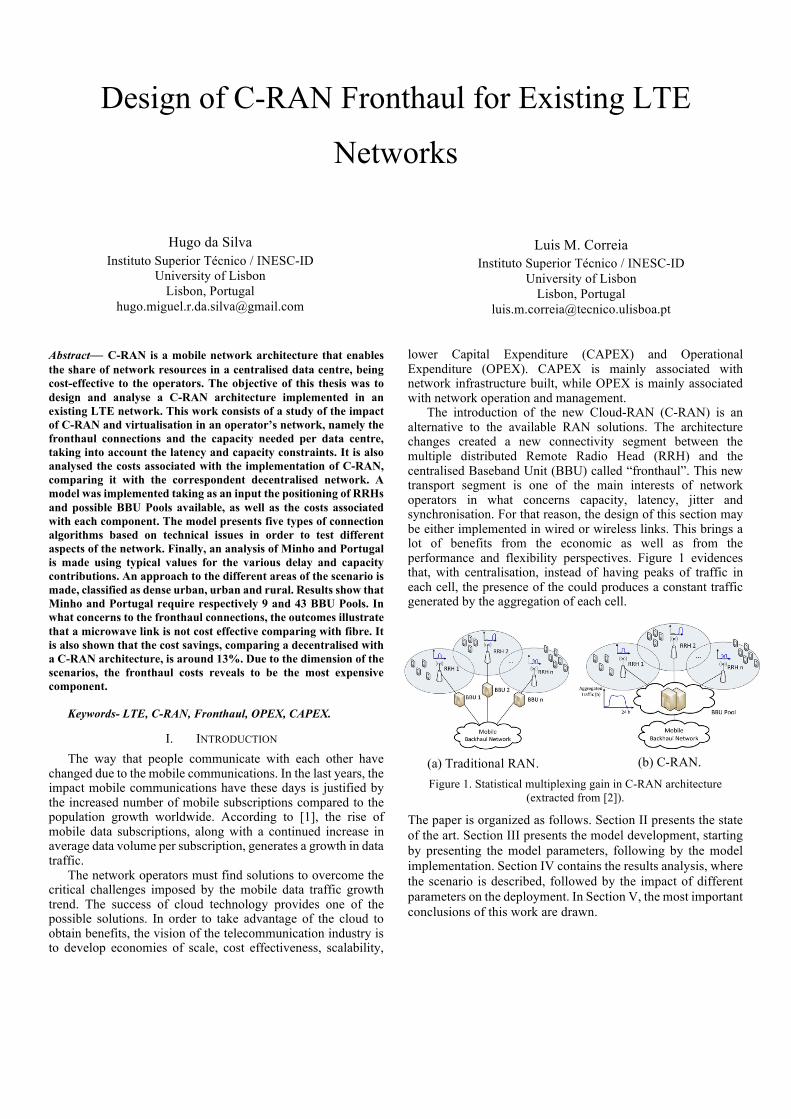
The introduction of the new Cloud-RAN (C-RAN) is an alternative to the available RAN solutions. The architecture changes created a new connectivity segment between the multiple distributed Remote Radio Head (RRH) and the centralised Baseband Unit (BBU) called “fronthaul”. This new transport segment is one of the main interests of network operators in what concerns capacity, latency, jitter and synchronisation. For that reason, the design of this section may be either implemented in wired or wireless links. This brings a lot of benefits from the economic as well as from the performance and flexibility perspectives. Figure 1 evidences that, with centralisation, instead of having peaks of traffic in each cell, the presence of the could produces a constant traffic generated by the aggregation of each cell.
Figure 1. Statistical multiplexing gain in C-RAN architecture (extracted from [2]).
The paper is organized as follows. Section II presents the state of the art. Section III presents the model development, starting by presenting the model parameters, following by the model implementation. Section IV contains the results analysis, where the scenario is described, followed by the impact of different parameters on the deployment. In Section V, the most important conclusions of this work are drawn.
(b) C-RAN. (a) Traditional RAN.
II. STATE OF THE ART The potential of Heterogeneous Networks (HetNets) has
been proved to satisfy the increasing data rates, proximity to end user, efficient spatial spectrum reuse and indoor coverage. According to [3], the most efficient physical link in the fronthaul of HetNet is Radio-over-Fibre (RoF). It simplifies the distribution of Millimetre-Wave (MMW) signals, which minimise interference with existing wireless services in HetNet. To support MMW small cells, the authors propose a local centralised optical Coordinated Multipoint (CoMP) thought RoF fronthaul using only local information and local high capacity RoF links.
[4] also presents an approach focused on the fibre - MMW link. The experimental results show that the effect of fibre dispersion is negligible when the fibre length is shorter than 50 km. The MMW-wireless link was limited to 3 m because of space limitations and because it was used a low-gain antenna. Nevertheless, it is expected that it can be significantly increased to an appropriately long range if a high-gain antenna is used. This technology is an attractive method for realising broadband radio signal delivery where broadband wireless infrastructure and fibre cables are not available.
The traffic distribution can change in case new cells are added to the network or if existing cells change their traffic profile. Therefore, [5] proposes using a packet-based fronthaul based on Ethernet that RRHs can be dynamically assigned to BBU Pools. Consequently, the overall multiplexing gain of the BBU Pools can be maximised. The optimal gain can be obtained connecting 20-30% of office base stations and 70-80% of residential base stations to the BBU Pool.
Besides consuming power for operation, support equipment sites remain unused as traffic load varies throughout the day. For that reason, [6] states that, unless the mobile operator already owns large fibre infrastructure, deployment of fibre exclusively for C-RAN may not be cost-effective unless a majority of sites remain served by microwave radio. The cost of fibre in a C-RAN deployment constitutes one of the largest CAPEX components, then, to solve this issue, the usage of microwave radio to replace fibre is warranted for population densities of over 8000 users/km2 when considering cheap fibre.
Cloud computing and virtualisation techniques are considered an opportunity to reduce operation costs and provide flexible and dynamic systems. For that reason, [7] focus on multiplexing gains induced from user load and data traffic heterogeneity. Here, the evaluation shows the increase of the multiplexing gain when a higher number of sectors are aggregated in a single fronthaul link. In fact, the aggregation of five sectors saves 9% of the compute resources.
From an economical viewpoint, [8] proposes a model to compare the local BBU with three strategies for BBU hoteling, such as BBU staking, BBU Pooling and C-RAN. The model includes cost comparisons and sensitivity analysis with respect to pooling and virtualisation gain. A scenario handling 100 cells was created to do the assessment of the model. In terms of relative cost, the CAPEX and OPEX decreases as the level of resource sharing increases.
Due to user mobility and network usage, the traffic load in mobile networks is an issue to take into consideration the variations during the day. Therefore, [9] presents the energy and cost savings in C-RAN are evaluated numerically using OPNET.
Here, a real case scenario was built upon the mobile traffic forecast for the year 2017. It is stated that C-RAN enables reduction of user data signal processing resources 4 times comparing with the traditional architecture.
The cost issues related to deploying C-RAN was investigated by [10] in order to find the most feasible configurations and choice of technologies. The model proposed minimises the length of fibre while at the same time maximises the statistical multiplexing gain for each BBU Pool.
III. MODEL DEVELOPMENT
A. Model Overview The main objective of this thesis is to develop and study a
solution for C-RAN implementation in a certain area with a focus on the fronthaul link, whether it be through fibre or microwave, which is the key aspect related to the investment [6]. The model pretends to analyse the network configuration with different specifications, regardless of the scenario of study, in order to get a weighed result. The model can be basically divided into three layers: • Physical. • Technical. • Costs. The first layer aims at computing the distances between the
RRHs and the BBUs. Associated to the calculation, the possible connections that one RRH can have with all the BBUs are also computed. This assignment is made based on the maximum latency that a fronthaul link can have, taking into account the different propagation velocities both in fibre and in microwave links.
The second layer deals with five different algorithms, highlighted in Subsection III.D: • Minimise Delay. • Number of RRH per BBU Balance. • Minimise Number of BBU Pools. • Flatness. • Capacity Load Balance. This layer is responsible for determine the most accurate
assignment within the existing possibilities, taking into account the algorithm. The different algorithms focus on different network aspects such as fronthaul distance and delay, number of RRH that one BBU handle, the number of BBUs used, the traffic load of each RRH and consequently of each BBU and the capacity of the BBU. After weighting the options, the model produces the connections between RRHs sites and BBU Pools ones.
The costs layer is divided in two more layers, each one with steps. One layer is related with CAPEX and the other with OPEX.
B. Model Parameters 1) Latency
There are several applications that do not require a very high data rate but require a very low delay. Latency is one of the main constraints for the fronthaul in a C-RAN architecture. This parameter determines the maximum length of the link between RRH and BBU Pool.
It is important to note that usually latency is represented by the measure of Round Trip Time (RTT), which has a more meaningful impact on Quality of Experience (QoE) than One-Way Delay (OWD). For simplicity, the present work assumes that RTT is given by: δ"## = 2 ∙ δ'() (1)
The length of the fronthaul link is dictated by its characteristic speed and by the fronthaul OWD, hence: d+,-./0123 56 = v[56/6:] ∙ δ+,-./0123[6:] (2)
where: • d+,-./0123 – Fronthaul distance. • 𝑣 – Transmission speed in the link. • δ+,-./0123 – Fronthaul OWD.
Equation (2) can also be used to obtain the RTT in the fronthaul as a function of the length of the fronthaul link.
Splitting the Base Station (BS) functionalities between BBUs and RRHs and centralising BBUs into few hotels brings many benefits, in terms of costs and RAN performance. However, this requires a proper network to transport the new fronthaul traffic, exchanged by BBUs and RRHs [11], in addition to the conventional backhaul traffic. Transporting fronthaul traffic over access networks is critical from the latency point of view. Strict latency constraints must be met when transporting fronthaul. Thus the physical distance between BBUs and RRHs is limited and a trade-off between higher BBU consolidation and fronthaul latency requirements arises.
As specified in [12], a maximum total round-trip latency δ"##,>>?@""A is 2ms. Regarding different latency contributions, the following condition must be held: δ"##,>>?@""A = 2δ+,-./0123 + δ""A,?C + δ>>?,?C
The maximum δ"##,>>?@""A directly translates to a maximum admissible OWD for every Common Public Radio Interface (CPRI) flow or, equivalently, to a maximum length of its route. The range of maximum length is typically between 20 and 40 km [13].
2) Cost Functions Due to the centralisation, collateral systems, such as
cabinets, racks, the power supplying, cooling, and aggregation gateways, can be re-implemented to save energy and costs. Cloud computing and virtualisation, technologies introduced on a C-RAN approach, provide an effective way to share the processing resources.
In order to face the high traffic demand that requires an increase in computational resources and transmission capacity, mobile operators are investigating novel solutions for cost-effective network expansion and upgrade. In [8], it is proposed a model to compare, in terms of costs, the local BBUs and the
three different strategies for BBU hoteling: BBU stacking, BBU Pooling, and C-RAN.
Given that the obtainable data do not fulfil all the parameters of the cost model proposed by [8], which are related to specific components and technology unknown at the time being, it was necessary to make some changes in order to adapt to the information available.
The adapted model is divided into two main costs functions, one for CAPEX and the other for OPEX. 𝐶JKLMN[€] = 𝐶PQRST[€] + 𝑁VWMXY𝐶ZRST[€/[\1,] (4)
where: • 𝐶JKLMN – Total cost of the architecture. • 𝐶PQRST – Total cost of CAPEX. • 𝐶ZRST – Total cost of OPEX per year. • 𝑁VWMXY – Number of years considered for OPEX. The adjustment just takes into consideration the recent
technology available in the network (local) and the futuristic one (C-RAN), which are the first and the last proposed by [8], respectively.
The aspects to take into account for the CAPEX calculation are the cost of the hardware, licences and civil works. In this way, the costs for the local architecture is: 𝐶PQRST,NK]MN[€] = 𝑁^^_`𝐶^^_`[€] + 𝑁^^a`𝐶^^a`[€]
where: • 𝐶PQRST,NK]MN – Cost of CAPEX for a local architecture. • 𝐶^^_`/a` – Cost of construction of a 10/20MHz cell. • 𝐶PMbcdWL,NK]MN – Cost of a local cabinet. • 𝐶YcLW,NK]MN – Cost of a local site. • 𝐶ecbWX – Cost of dark fibre per kilometre. • 𝑁^^_`/a` – Number of 10/20MHz cells. • 𝑁]Mb,N – Number of aggregation points in a local
architecture. • 𝑁YcLW – Number of sites. • 𝑁eN – Number of kilometres of the fibre link. Since that the C-RAN architecture have a virtualisation
approach and an additional cost for the fronthaul, the CAPEX cost is: 𝐶PQRST,P@hQi[€] = 𝑉 𝑁^^_`𝐶^^_`[€] + 𝑁^^a`𝐶^^a`[€]
architecture. • 𝐶PMbcdWL,P@hQi – Cost of a C-RAN cabinet. • 𝐶YcLW,P@hQi – Cost of a C-RAN site. • 𝐶gc]XKkMlW – Cost of microwave equipment. • 𝑁]Mb,] – Number of aggregation points in a C-RAN
architecture. • 𝑁gN – Number of the microwave link. • 𝑉 – Virtualisation factor.
In what concerns to project the fixed costs every year, the OPEX takes into consideration three main factors: 𝐶ZRST[€] = 𝐶WdWXmV[€] + 𝐶XWdLcdm[€] + 𝐶gMcdLdWd]W[€]
+ 𝐶ecbeXKdLnMoN[€] + 𝐶gkNc]Wd]WY[€] (7)
where: • 𝐶WdWXmV – Cost of the energy consumption. • 𝐶XWdLcdm – Cost of renting. • 𝐶gMcdLdWd]W – Cost of a maintenance of infrastructures. • 𝐶ecbeXKdLnMoN – Cost of maintenance of fibre fronthaul. • 𝐶gkNc]Wd]WY – Cost of microwave fronthaul licences. The energy consumption is related to air-conditioning and
telecom equipment associated for each RRH to BBU connection. The virtualisation in a local approach is 1. This factor exists in a C-RAN architecture, which has energy savings due to the centralisation. 𝐶\.\,p[[€] = 24 ∙ 365𝐸>>? 5(0 𝐶+\\ €/(5(0) 𝑁""A,w-.𝑉 (8) where: • 𝐸^^x – Energy consumed per hour for a BBU. • 𝐶eWW – Energy fee. • 𝑁hhy,]Kd – Number of RRH connected. The feature related with renting takes into consideration the
average price per m2 per month in different areas: 𝐶XWdLcdm[€] = 12[6-./0]𝐴[6|]𝑉 𝑁}x𝐶}x[€/6|/6-./0]
+ 𝑁x𝐶x[€/6|/6-./0]+ 𝑁h𝐶h[€/6|/6-./0]
(9)
where: • 𝐶}x/x/h – Cost of rent a square metre per month in a
dense urban/urban/rural area. • 𝑁}x/x/h – Number of RRHs in a dense urban/urban/rural
area. • 𝐴 – Area occupied by an RRH. The conditions that allow the prediction of the maintenance
are related to the deployment of the network, the hardware that is not related to the baseband processing and the computer boards responsible for deal with signal processing. For that reason, maintenance is computed by a multiplication between the different aspects of CAPEX and different coefficients. 𝐶gMcdLdWd]W[€] = 0.01𝐶PQRST,�W�NKVgWdL[€]
+ 0.1𝐶PQRST,nMX�kMXW[€]+ 0.25𝐶PQRST,]Kg�oLWX[€]
(10)
where: • 𝐶PQRST,�W�NKVgWdL – Cost of deployment investment. • 𝐶PQRST,nMX�kMXW – Cost of hardware investment. • 𝐶PQRST,]Kg�oLWX – Cost of computer investment. The fibre infrastructure also requires maintenance, which is
a percentage of the investment in fibre links: 𝐶ecbeXKdLnMoN[€] = 0.06𝑁eN[56]𝐶ecbXW[€/56] (11)
To compute the licences costs due to the microwave transmission it is necessary to consider three factors: the distance of the link, the frequency band of transmission and the bandwidth used. One should consider also a Cross Polarisation Cancellation Interface (XPCI) factor. 𝐶gkNc]Wd]WY[€]
= 𝑘_[€/�A�/ 56] 𝑑eXKdLnMoN[56]𝐵[�A�]ϕ���� (12)
where: • 𝑘_ – Factor related with the bandwidth. • 𝐵 – Bandwidth. • ϕ���� – XPCI factor. 3) Multiplexing Gain
To evaluate the performance of the C-RAN architecture in what concerns to traffic fluctuations, [5] proposes a metric to weigh the benefits from the statistical multiplexing gain viewpoint. The statistical multiplexing gain compares resources needed in a traditional RAN to resources needed in a C-RAN. As the number of baseband resources are proportional to the traffic they need to process, it is compared the sum of the traffic peaks in a traditional RAN to the peak in a BBU Pool in a C-RAN:
𝐺go� =𝑇�WMf,c[�>/0]
������_
𝑇�WMf,�[�>/0]������_
(13)
where: • 𝑁hhy – Number of RRHs. • 𝑇�WMf – Peak of traffic during the day.
C. Model Implementation The model has the objective of analysing the network
configuration, based on locations and traffic profile, to better understand the fronthaul connections and the type of fronthaul links deployed over a C-RAN architecture. In Figure 2, it is possible to analyse a detailed perspective of the overall workflow of the model.
Figure 2. Model Flowchart.
D. Algorithms To illustrate how the algorithms work, a scenario with 2
BBU Pools and 10 RRHs was created, being assumed that both BBU Pools do not have capacity limits and that all RRHs can connect to both BBU Pools, which means that there are no restrictions concerning distance/latency.
The first four algorithms have the same principle, differing in the key aspect to analyse. There are three kinds of RRHs, based on the maximum fronthaul distance, in what concerns to number of possible BBU Pools connections: • The ones that cannot be connected to any BBU Pool,
which means that do not respect the distance requirement.
• The ones that may be connected to one BBU Pool, which means that they just respect the distance requirement to that BBU Pool.
• The ones that respect the distance requirement to more than one BBU Pool, which means that they will ponder the options to may connect to the most appropriate BBU Pool for each algorithm.
To connect an RRH to an BBU Pool, there are two network requirements that must be fulfilled: the first is maximum fronthaul distance and the second is the maximum capacity of the BBU Pool, both specified by the input parameters. Thus, the RRHs that do not respect at least one of the restrictions cannot be connected to any BBU Pool. For that reason, they will have their own BBU decentralised, which means that the BBU stays as in the traditional RAN.
1) Minimise Delay The Minimise Delay Algorithm aims to connect the RRH
closer to the possible BBU Pool location, Figure 3. Each RRH has possible locations of BBU Pools to connect. Thus, knowing all the distance between that possible connections, the RRH will check the capacity requirement to the nearest BBU Pool until it is able to start the connection.
Figure 3. Minimise Delay algorithm diagram.
2) Number of RRH per BBU Balance The Number of RRH per BBU Balance Algorithm aims to
equilibrate the number of RRHs in every BBU Pools, Figure 4. The information of the number of RRH that each BBU Pool have is always available and updated. In this way, each RRH, before pondering the decision, has the information to analyse the possible connections. Thus, the RRH will check the maximum capacity of the BBU Pool with less RRHs already connected until it is capable of start the connection. With this approach, it is guaranteed that the BBU Pools have almost same number of RRHs.
Figure 4. Number of RRH per BBU Balance algorithm diagram.
3) Flatness The Flatness Algorithm aims to force a horizontal traffic
profile in every BBU Pools, Figure 5. This approach has the objective to avoid peaks of traffic. Taking into consideration the three types of RRHs: residential, commercial and mixed. Those have specific time intervals throughout the day with traffic. The ideal BBU Pool traffic profile should have a constant traffic load throughout the day in order to obtain multiplexing gains and energy efficiency in a C-RAN approach comparing with the
traditional RAN. The algorithm takes the hours of the day selected at the input parameters. That hours must be a vector of integers ranging between 1 and 24, which can have any size.
Knowing that the information of the traffic profile of each BBU Pool is always updated, each RRH will evaluate the possible connections. This evaluation is based on the vector of hours. The RRH, before connect to one BBU Pool considers the traffic load, assuming that the connection is made, doing a linear regression on the points of time of the vector. The linear regression that has lower slope is the one that provides higher gains. Thus, until there are no more BBU Pools to analyse and taking into consideration the maximum capacity limit of each BBU Pool, the RRH will start the connection with the BBU Pool with lower slope provided by the linear regression. With this decision, it is ensured that the BBU Pools will have constant traffic throughout the day.
Figure 5. Flatness algorithm diagram.
4) Capacity Load Balance The Capacity Load Balance Algorithm aims to equilibrate
the traffic load in every BBU Pool, Figure 6. The information of traffic load of each BBU Pool is always available and updated. Before pondering the decision, each RRH has the information of traffic of the possible BBU Pools connections. Thus, the RRH will check not only maximum capacity limit of the BBU Pool but also the possible load if the connection occurs. The possible BBU Pool connection that has the lower traffic load after the link happens starts the connection. With this approach, it is guaranteed that the BBU Pools have a balance in what concerns to traffic load.
5) Minimise Number of BBU Pools The Minimise Number of BBU Pools Algorithm aims to
minimise the number of BBUs that are used, Figure 7. The key aspect of this algorithm is to understand, for each RRH, the possible BBU Pools that are already in use. This information is always available and updated. There are three hypotheses of number of possibilities, based on number of BBU Pools that are already in use for each RRH: • The RRHs that only can connect to one BBU Pool
already in use, which means that the RRHs may be connected to that BBU Pool.
• The RRHs that can connect to more than one BBU Pool already in use, which means that the RRHs will weigh the options to may connect to the most appropriate BBU Pool.
• The RRHs that cannot connect to any BBU Pool already in use, which means that the RRHs will ponder the options and may connect to an unused BBU Pool.
To ponder the connections to the ones that have more than one possibility, the RRHs check the maximum capacity limit of each possibility and connect to the one that has a traffic load flatness, based on the third algorithm. The remain ones that does not have possibilities to connect to one BBU Pool already in use are forced to connect to the BBU Pool that has the possibilities to connect the larger number of RRHs. With this approach it is guaranteed that the number of BBU Pools is minimised. The RRHs that does not respect at least one of the requirements, distance or capacity limits, cannot be connected to any BBU Pool. For that reason, they will have their own BBU decentralised, which means that the BBU stays as in the traditional RAN.
Figure 7. Minimise Number of BBU Pools algorithm diagram.
IV. RESULTS ANALYSIS
A. Scenarios To study the performance of a C-RAN architecture when it
is implemented on a large scale, this thesis has two different scenarios: • Minho, in which all the data was provided by NOS, such
as the possible locations of the BBU Pools and the location of the RRHs with the respective traffic data. This scenario has 374 cell sites, 1 176 RRHs and 42 possible BBU Pools.
• Portugal, illustrated in Figure 8, in which the possible locations of the BBU Pools are pondered all over the country based on the NOS stores, the RRHs locations provided by NOS and the traffic load was extrapolated from the data from the previous scenario. This scenario has 2 755 cell sites, 8 065 RRHs and 86 possible BBU Pools.
Figure 8. Portugal map with RRHs and possible BBU Pools
locations.
To classify the RRHs for areas, such as dense urban, urban and rural, one has established metrics based on the density of RRH. Analysing the number of neighbours in a 2 km radius, it was defined two thresholds to split the three types of areas justified by empirical tests to correspond to a real case scenario.
In what concerns to the traffic profile of the RRHs, considering that the day has 24 hours, there are three intervals to analyse: • Dawn – between 00:00 and 08:00. • Labour – between 08:00 and 17:00. • Night – between 17:00 and 00:00. The RRHs are divided into three classifications according to
the hours of the day with higher traffic load: • Commercial – if the traffic in the labour period
substantially higher comparing with the night. • Residential – if the traffic in the night period substantially
higher comparing with the labour. • Mixed – if the difference between the traffic in the labour
and the night period is not significant.
B. Analysis of Minho Scenario 1) Latency Impact
The first insight that one can extract from the latency is the expected decrease in the percentage of dense urban RRHs and an increase in the percentage of rural RRHs as the maximum fronthaul delay increases. The Figure 9 depicts this evolution of the percentage of RRHs type of area, according to the capacity balance algorithm. The figure also illustrates a dominance on rural RRHs above 10 km of the radius with the centre in the BBU Pool positions. One can clearly understand that with the increase of the percentage of connected RRHs, the rural ones can also increase with the same trend. One should notice that are BBU Pools in rural areas which means that the centralisation in a denser scenario may have a different tendency.
Figure 9 Area type of shared RRHs with different fronthaul distances in Minho.
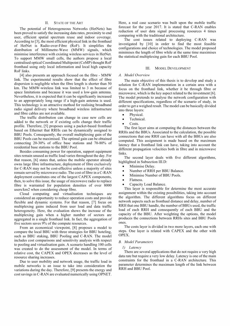
The manipulation of the maximum fronthaul distance constraint has a direct impact on the multiplexing gain. Figure 10 shows, with the capacity balance algorithm, the variation of user multiplexing gain in BBU Pools positioned in dense urban, urban and rural areas considering the fronthaul link length. The classification of dense urban, urban and rural BBU Pool was made based on the percentage of dense urban, urban and rural RRHs that are connected to that BBU Pool. Each BBU Pool is classified according to the higher percentage of the connected RRHs type. One can easily see that the total multiplexing gain do not have a significant variation, only 3% when the fronthaul distance increases. This behaviour reaches a maximum value between the 4 and 6 km and a minimum at 16km. This fact is justified by the distribution of commercial, residential and mixed traffic, that are represented in Figure 11. Here, when the percentage of mixed RRHs increases, the total multiplexing gain decreases. This algorithm is computed to make the BBU Pools balanced in terms of traffic and, as the fronthaul distance increases, the percentage of mixed RRHs also increases. This
kind of RRHs, having a non-well established traffic profile when connected, introduces a negative impact in terms of multiplexing gain. Since the dense urban percentage decreases, as illustrated in Figure 9, the percentage of BBU Pools characterised as dense urban also decreases. Consequently, the multiplexing gain in dense urban BBU Pools decreases. The multiplexing gain in urban BBU Pools reaches a maximum value, at 4 km, when the percentage of urban RRHs also reaches his maximum. After that, the gain remains almost constant varying 2% as the fronthaul distance increases. As expected, the rural BBU Pools have a minimum gain at 2 km, where the existence of rural RRHs is at a reduced number. The majority of rural RRHs have mixed traffic profile. For that reason, as far as the fronthaul distance increases as well as the percentage of rural RRHs and consequently the mixed RRHs, the multiplexing gain remain with the same trend, having a variation of almost 2%.
Figure 10. Multiplexing gain in variation for different fronthaul distances.
Figure 11. Traffic type of shared RRHs with different fronthaul distances.
It is expected a decrease in the percentage of possible microwave links caused by the increasing of the maximum fronthaul distance. This possibility is an option that occurs when the fronthaul distance is below 1.5 km, assuming that are a line of sight. It is important to understand the different behaviours of Minimise Delay and capacity balance algorithms. In fact, Figure 12 shows that, as the maximum distance increases from 10 km to 40 km, the percentage of possible microwave links decreases approximately 5% in both algorithms. This means that the saturation of the percentage of possible microwave fronthaul links starts at the 10km. In the Minimise Delay algorithm, once that the connections are made between the BBU Pool to the closer RRH it is guaranteed that above the 1.5 km all the possible microwave fronthauls are established at the first point of the graph. As the maximum fronthaul increases the number of connections also increases justifying the decrease of percentage in microwave links. However, using the capacity balance algorithm, the connections do not have a specific trend in what concerns to distance variation. In this algorithm, between some points, the tendency is contrary to the descending trend. Increasing the maximum distance imposed, each BBU Pool may have more possible RRHs to connect. The additional possibilities provided by the increasing of the fronthaul distance
are above the 1.5 km, but each BBU Pool already has possibilities below the 1.5 km. The algorithm allows a balance distribution in capacity between BBU Pools. For that reason, to increase the distance constraint, the number of possible connections per BBU Pool may also increase, providing more options to do a more balanced network, not considering the fronthaul distance in the decision. If one considers that microwave technology could only support the traffic demand of the considered RRHs for shorter distances (e.g., 1 km or less), it would reduce these percentages, even if the curve should exhibit a similar behaviour. Here, a polynomial model is used for the fitting, since it was the one with the higher correlation R2.
Figure 12 Shared possible microwave links for different
fronthaul distance.
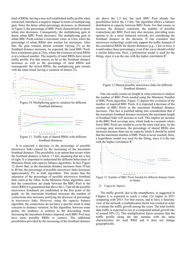
One can easily extract an insight in what concerns to analyse the number of BBU Pools needed using the Minimise Number of BBU Pools algorithm. Figure 13 depicts this evolution of the number of required BBU Pools. It is expected a decrease of the number of BBU Pools as the maximum fronthaul distance increases. This fact is justified taking into consideration that if the maximum fronthaul distance increases, the maximum length of fronthaul links will increase as well. This implies an increase in the BBU Pool coverage area, which leads to a scenario where fewer BBU Pools are needed to cover the same total area. As the coverage area increases, the percentage of shared RRHs also increases because there are no capacity limits It should be noted that the maximum number of BBU Pools is never reached. Here, a logarithmic model was used for the fitting, since it is the one with the higher correlation R2.
Figure 13. Number of BBU Pools Needed for different distance limits
in Minho.
2) Capacity Impact
The traffic growth, due to the smartphones, as suggested in Chapter I, is expected to reach a value 12x higher in 2021 comparing with 2015. For that reason, and to have a futuristic view of the network, a multiplication factor was created in order to evaluate the traffic growth among the years. The total mobile data traffic is expected to rise at a compound annual growth rate of around 50% [1]. This multiplication factor assumes that the traffic profile along the day remains with the same characteristics for each RRH and it does not change geographically.
Table 1. Traffic multiplication factor among the years.
The maximum capacity of a BBU Pool needs to be dimensioned with a margin considering the planned consumption, allowing to deal with higher traffic peaks if they occur and to account with forecasted traffic growth, as Figure 14 suggests. The figure shows, using the capacity balance algorithm, not only the maximum traffic of the BBU Pool with the highest peak of traffic but also the maximum traffic of the BBU Pool with the lowest peak of traffic. One should note that the figure does not take into consideration with the margin. That need to be considered by the operator and it is a percentage of the maximum peak of traffic. Usually, this margin takes percentages between 10% and 20%. Here, the fitting represents an exponential model with R2=1, which proves that the two quantities are directly proportional as it was intuitively expected.
Figure 14. Maximum and minimum traffic variation in the BBU
Pools for until 2021.
When BBUs are aggregated in a BBU Pool, such a margin can be shared, allowing additional pooling gain in C-RAN architecture comparing to a traditional RAN. In Figure 15, it can be seen that establishing a limit of capacity per BBU Pool, the network take advantage of that possibility, reaching almost the maximum value. From 5 GB/h to 30 GB/h, the maximum capacity is almost equal to the maximum established, but with 50 GB/h the margin is 8%. For that reason, such an additional margin is especially applicable to resources required to support traffic peaks in different cells. In other words, in C-RAN, the capacity can be scaled and dimensioned based on peak utilisation in all BBU Pool, rather than all RRHs peak utilisation.
Figure 15. Maximum and minimum traffic for different capacity limits per BBU Pool.
3) Costs analysis The CAPEX and OPEX are important parameters when a
network is deployed. As it can be seen in Figure 16, adopting the proposed model, the CAPEX cost reduction using a C-RAN instead of a traditional RAN is 14% considering the haul component and 51% not considering the investment in this connections. The main component of CAPEX analysis is, as
expected, the haul. The backhaul has almost the same cost as the fronthaul. Nevertheless, comparing the local with C-RAN architecture, the haul increases around 0.2% due to the fronthaul microwave links. The fact that the microwave link can only be established for distances below 1.5 km contributes to the increasing cost. Since each microwave link costs 12 000 € and one kilometre of fibre costs 6 000 €, the fibre links are advantageous from an economical viewpoint for distances bellow 2 km. The haul factor, due to the expensive cost of fibre in long distances, appears as the most significant element even though it is assumed that the mobile operator owns 85% of the infrastructure. Furthermore, analysing the cost without the haul it is evident that the sites construction represents the CAPEX principal component. This is justified by the fact that the BS is the most expensive factors of a wireless network infrastructure. The variation of 59% in this element takes into consideration the difference in costs between a local and a C-RAN architecture assumed in the reference parameters. In what concerns to cabinets cost it is important to understand that, as expected, the cost increases 50% in C-RAN. Once that the price of a cabinet normalised per cell in C-RAN is 1.5 times higher than in a local architecture, it is expected that the total cost of this component remains with the same trend. In the BB component, the fact that the virtualisation factor is considered makes a 14% cost reduction in C-RAN comparing to the local. The virtualisation factor is the key feature in this component because the cost of a BB unit is the same in both architectures whether it be 10 MHz or 20 MHz cell.
Figure 16. Local and C-RAN CAPEX with its components in Minho.
The OPEX cost reduction using C-RAN instead of a traditional RAN, as Figure 17 suggests for one year, is 13% considering the haul component and 30% not considering these connections. Likewise, the CAPEX analysis, the most significant influence is also the haul because its value is a percentage of the initial investment considering the fibre, which is the most significant transmission link. Leaving aside matters related with the haul, the most obvious reduction is in the renting, around 37% due to the area considered to be occupied per cell in C-RAN is lower comparing with the local architecture. Moreover, the costs ratio in different geographical areas is also considered in renting factor, which also increases the savings. Justified by the fact that the reduction in power consumption between the two architectures is related with the virtualisation factor, the cost saving in energy is approximately 14%. The cost reduction of 17% in the maintenance component is based on the reduction of BB hardware and computers virtualised in the BBU Pools. This centralisation also influences the savings in what concerns to civil work.
Figure 17. Local and C-RAN OPEX per year with its components in Minho.
C. Analysis of Portugal Scenario Taking the possible 86 BBU Pools and considering that are
no capacity limits in any data centre, using the Minimise Number of BBU Pools algorithm, is illustrated in Figure 18 the number of BBU Pools used for different values of maximum fronthaul distance. As expected, the number of BBU Pools that are needed in the network decreasing trend as the maximum fronthaul distance increases. This behaviour happens because as the coverage areas increase the overlapped areas also increase, making some BBU Pools locations redundant to cover the same region. The minimum number of BBU Pools needed for Portugal are 44, almost 5 times more than in Minho. This number only allow the connection of 96,6% of the total RRHs. One should notice that the total number of BBU Pools never reaches the maximum number of possibilities and using less BBU Pools, the costs both in CAPEX and OPEX will rise due to the increase of the fronthaul links length. Here, a linear model was used for the fitting in both architectures, since it is the one with the higher correlation R2. It should be noted that increasing the scenario in 8 times, the number of possible BBU Pools only increase twice.
Figure 18. Number of BBU Pools Needed for different distance limits
in Portugal.
The key concern of a C-RAN dimensioning is to provide a network that is cost-effective for the operator, and this fact aggravates when the scenario is Portugal. Figure 19 illustrates the total CAPEX for a local and a C-RAN architecture. One should remember that haul refers to the backhaul in local and fronthaul in C-RAN. It is assumed in this comparison that the operator owns 85% of the haul infrastructure. The first insight that is taken from the figure is the 13% of cost savings using C-RAN. It is noticeable that the component with higher relevance is the haul, representing 78% and 90% of the total CAPEX in local and C-RAN, respectively. This component does not contribute positively to the savings, around 0.08% more expensive in C-RAN due the cost of the microwave fronthaul links in comparison with the correspondent fibre backhaul links. In fact, the most responsible factor for saving is the sites construction, which is 69%. This large percentage of savings are
related to the fact that in a local architecture, the cost of sites construction is, by reference, 3 times higher than in C-RAN. Being 1% of the total CAPEX in both architectures, the baseband component introduces 4% of savings introduced by the multiplexing gain, that exists in C-RAN in contrast with local. This low multiplexing and consequently, low percentage of saving in this component is justified by the fact that in this scenario only three curves of traffic are considered. This three traffic profile are based on the average traffic in Minho. So, the diversity of traffic profile is poor, which generates lows and unreal multiplexing gains. The cabinets component is characterised to be 1.5 times expensive in C-RAN comparing with local. Thereby, it represents a negative impact of 50% in terms of saving.
Figure 19. Local and C-RAN CAPEX with its components in Portugal.
Apart from the initial investment, it is important to keep the network providing a reasonable QoS for users along the years. In order to make it happen, a continuous investment is needed in order to maintain the network under the intended conditions. For that reason, Figure 20 suggests the OPEX per year in a local and in a C-RAN architecture. By analysing the figure, it is possible to see, as expected, a reduction in the OPEX using a C-RAN architecture comparing with local. This cost reduction represents 10% of cost savings. It is also evident that the main component in both architectures is the haul. Here, it is also assumed that the network operator owns 85% of the haul. This component represents 64% of the total CAPEX. Comparing the savings using C-RAN and using local, the haul represents a negative impact of 0.07% regarding that the licences of the fronthaul microwave links are high-priced than the maintenance of the correspondent backhaul fibre links. The component that introduces a high percentage of savings, approximately 38%, is the renting. As already discussed, the cost of a dense urban, urban and rural square metre, are respectively 1.15, 1.25 and 1.25 times higher in local comparing with C-RAN. When the scenario is Portugal, where the number of RRHs is relative to a country and the percentage of rural is higher than the sum of dense urban and urban, the savings in renting become notorious. The maintenance also contributes positively to the savings, having 15% of cost reduction. The influence of this component is related to the reduction in CAPEX sites construction. Although the sites construction is the component with the lower percentage in the maintenance, the fact that sites construction is the second most significant in factor in CAPEX contributes the savings in OPEX. As introduced in Subsection III.B.2, the differentiator feature in the energy component is the virtualisation factor. The fact that the traffic curves that are used in Portugal are based on the average curves of Minho, it creates only three types of traffic profiles. Thus, the multiplexing gain
generated is low and consequently, the virtualisation factor is near to,1 providing only a 4% savings in the energy.
Figure 20. Local and C-RAN OPEX per year with its components in Portugal.
V. CONCLUSIONS Regarding the locations of the RRHs, three classes of RRHs
were defined based on the geographical density of the RRHs, namely dense urban, urban and rural. Based on the traffic profile of each RRHs, also three classifications were made, namely commercial, residential and mixed. This classification is established by variation of the traffic along the day.
In Minho, as the maximum fronthaul distance increases from 2 km to 40 km, the percentage of connected RRHs also increases from 40% to 100%. The maximum overall multiplexing gain is obtained at 4 km, where the residential and commercial RRHs have a majority and the residential ones reach its maximum value. In this way, by having complementary curves, the gain is maximised to 1.15. In [5], the maximum multiplexing gain achievable is 1.6. In fact, only two types of traffic profiles, namely commercial and residential for every RRHs, are considered to connect just one BBU Pool. This shows that with a real case scenario, a vast diversity of traffic profiles and more BBU Pools, the multiplexing gain achievable decreases. In this way, the mixed cells, resulting from rural areas, is a drawback for the multiplexing gain. Nevertheless, in smaller scenarios, the multiplexing gain should be higher due to the diversity of traffic profiles.
Using the Minimise Delay algorithm, one can conclude that the percentage of microwave fronthaul links is always above with the reference algorithm, which is around 9% and 24% greater at 2km and 40km, respectively.
Testing the Minimise Number of BBU Pools algorithm, as the fronthaul distance increases, the number of required BBU Pools decreases. Justified by the overlapping of BBU Pools coverage areas, the scenario never uses all the 42 BBU Pools available, using only 31 and 9 BBU Pools, respectively at 2 km and 40 km of maximum fronthaul distance.
The traffic in 2021 will be 7.59 times higher comparing with 2016. Therefore, it is expected that in Minho scenario, using the capacity balance algorithm, the maximum capacity of the most loaded BBU Pool behaves proportionally to the growth rate, reaching a maximum of 350 GB/h in 2021.
Evaluating the costs associated with Minho scenario, there is 14% of CAPEX savings by comparing the C-RAN with local architecture. One should notice that is assumed that the operator owns 85% of the haul (backhaul in local and fronthaul in C-RAN) infrastructure. In this way, the investment is 8.6 and 7.4 million € in local and C-RAN, respectively. The annual OPEX
has a reduction of 13% considering the C-RAN architecture. This reduction is represented for an OPEX of 669 and 584 thousand € per year in local and C-RAN, respectively. In what concerns to the fronthaul connections, the outcomes illustrate that a microwave link is not cost effective comparing with fibre.
In Portugal, the CAPEX has the 13% of cost savings using C-RAN. Thus, the investment is 66.2 and 76.5 million € in local and C-RAN, respectively. As well as the cost savings percentage is higher comparing with Minho, the amount of money saved is also greater, being almost 9 times superior. The amount of money saved in Portugal assures the development of Minho scenario, and there is still money left. The OPEX presents 10% of cost savings. In local, the annual investment is around 5.6 million €. Considering the C-RAN architecture, the investment is approximately 4.9 million €. Although the percentage of savings decreases comparing with Minho, justified by the decrease of the multiplexing gain, the amount of money that is saved is around 8 times greater comparing both scenarios.
REFERENCES [1] Ericsson, Ericsson Mobility Report, Public Consultation, Lisbon,
Portugal, June 2015, (http://www.ericsson.com/mobility-report). [2] A. Checko, H.L. Christiansen, Y. Yan, L. Scolari, G. Kardaras, M.S.
Berger and L. Dittmann, “Cloud RAN for Mobile Networks—A Technology Overview”, IEEE Communications Surveys & Tutorials, Vol. 17, No. 1, Sep. 2014, pp. 405-426 (http://ieeexplore.ieee.org/ stamp/stamp.jsp?tp=&arnumber=6897914).
[3] L. Cheng, C. Liu, M. Zhu, J. Wang and G.K. Chang, “Optical CoMP Transmission in Millimeter-Wave Small Cells for Mobile Fronthaul”, Optical Fiber Communications Conference (OFC), San Francisco, CA, USA, Mar. 2014 .
[4] P. Dat, A. Kanno, N. Yamamoto and T. Kawanishi, “Full-Duplex Transmission of LTE-A Carrier Aggregation Signal over a Bidirectional Seamless Fiber-Millimeter-Wave System”, J. Lightwave Technol., Aug. 2015.
[5] A. Checko, H. Holm and H. Christiansen, “Optimizing Small Cell Deployment by the Use of C-RANs”,Proc. Of 20th European Wireless Conference - European Wireless 2014, Barcelona, Spain, May 2014.
[6] R. Al-obaidi, A. Checko, H. Holm and H. Christiansen, “Optimizing Cloud-RAN Deployments in Real-Life Scenarios Using Microwave Radio”, European Conference On Networks and Communications (EuCNC), Paris, France, June 2015.
[7] T. Werthmann, H. Grob-Lipski and M. Proebster, “Multiplexing Gains Achieved in Pools of Baseband Computation Units in 4G Cellular Networks”, PIMRC, 2013 IEEE 24th International Symposium, London, United Kingdom, Sep. 2013.
[8] M. Andrade, M. Tornatore, A. Pattavina, A. Hamidian and K. Grobe, “Cost Models for Baseband Unit (BBU) Hotelling: from Local to Cloud”, CloudNet, 2015 IEEE 4th International Conference on Cloud Networking, Niagara Falls, ON, Canada, Oct. 2015.
[9] A. Checko, H. Christiansen and M. Berger, “Evaluation of energy and cost savings in mobile Cloud Ran”, in Proc. of OPNETWORK 2013, Washington, D.C., USA, Aug. 2014.
[10] H. Holm, A. Checko, R. Al-obaidi and H. Christiansen, “Optimal Assignment of Cells in C-RAN Deployments with Multiple BBU Pools”, in Proc. of EuCNC’15 – 24th European Conference on Networks and Communications, Paris, France, June 2015.
[11] A. Pizzinat, P. Chanclou, F. Saliou and T. Diallo, “Things you Should Know About Fronthaul”, Journal of Lightwave Technology, Vol. 33, No. 5, Jan. 2015, pp. 1077-1083.
[12] 3GPP, Technical Specification Group Services and System Aspects, Quality of Service (QoS) Concept and Architecture (Release 12), Report TS 23.107, V12.0.0, Sep. 2014 (http://www.3gpp.org/ftp/Specs/html-info/23107.htm)
[13] F. Musumeci, C. Bellanzon, N. Carapellese, M. Tornatore, A. Pattavina and S. Gosselin, “Optimal BBU Placement for 5G C-RAN Deployment Over WDM Aggregation Networks”, Journal of Lightwave Technology, Vol. 34, No. 8, April 2015, pp. 1963-1970