General rights Copyright and moral rights for the publications made accessible in the public portal are retained by the authors and/or other copyright owners and it is a condition of accessing publications that users recognise and abide by the legal requirements associated with these rights. Users may download and print one copy of any publication from the public portal for the purpose of private study or research. You may not further distribute the material or use it for any profit-making activity or commercial gain You may freely distribute the URL identifying the publication in the public portal If you believe that this document breaches copyright please contact us providing details, and we will remove access to the work immediately and investigate your claim. Downloaded from orbit.dtu.dk on: May 02, 2020 Design of Computer Experiments Dehlendorff, Christian Publication date: 2010 Document Version Publisher's PDF, also known as Version of record Link back to DTU Orbit Citation (APA): Dehlendorff, C. (2010). Design of Computer Experiments. Kgs. Lyngby, Denmark: Technical University of Denmark. IMM-PHD-2010-237
Transcript
General rights Copyright and moral rights for the publications made accessible in the public portal are retained by the authors and/or other copyright owners and it is a condition of accessing publications that users recognise and abide by the legal requirements associated with these rights.
Users may download and print one copy of any publication from the public portal for the purpose of private study or research.
You may not further distribute the material or use it for any profit-making activity or commercial gain
You may freely distribute the URL identifying the publication in the public portal If you believe that this document breaches copyright please contact us providing details, and we will remove access to the work immediately and investigate your claim.
Downloaded from orbit.dtu.dk on: May 02, 2020
Design of Computer Experiments
Dehlendorff, Christian
Publication date:2010
Document VersionPublisher's PDF, also known as Version of record
Link back to DTU Orbit
Citation (APA):Dehlendorff, C. (2010). Design of Computer Experiments. Kgs. Lyngby, Denmark: Technical University ofDenmark. IMM-PHD-2010-237
Technical University of DenmarkInformatics and Mathematical ModellingBuilding 321, DK-2800 Kongens Lyngby, DenmarkPhone +45 45253351, Fax +45 [email protected]
IMM-PHD: ISSN
Summary
The main topic of this thesis is design and analysis of computer and simulationexperiments and is dealt with in six papers and a summary report.
Simulation and computer models have in recent years received increasingly moreattention due to their increasing complexity and usability. Software packagesmake the development of rather complicated computer models using predefinedbuilding blocks possible. This implies that the range of phenomenas that areanalyzed by means of a computer model has expanded significantly. As thecomplexity grows so does the need for efficient experimental designs and analysismethods, since the complex computer models often are expensive to use in termsof computer time.
The choice of performance parameter is an important part of the analysis ofcomputer and simulation models and Paper A introduces a new statistic forwaiting times in health care units. The statistic is a measure of the extentof long waiting times, which are known both to be the most bothersome andto have the greatest impact on patient satisfaction. A simulation model foran orthopedic surgical unit at a hospital illustrates the benefits of using themeasure.
Another important consideration in connection to simulation models is the de-sign of experiments, which is the decision of which of the possible configurationsof the simulation model that should be tested. Since the possible configurationsare numerous and the time to test a single configuration may take minutes orhours of computer time, the number of configurations that can be tested is lim-ited. Papers B and C introduce a novel experimental plan for simulation models
ii
having two types of input factors. The plan differentiates between factors thatcan be controlled in both the simulation model and the physical system and fac-tors that are only controllable in the simulation model but simply observed inthe physical system. Factors that only are controllable in the simulation modelare called uncontrollable factors and they correspond to the environmental fac-tors influencing the physical system. Applying the experimental framework onthe simulation model in Paper A shows that the effects of changes in the un-controllable factors are better understood with the proposed design comparedto the alternative and commonly used methods.
In papers D and E a modeling framework for analyzing simulation models withmultiple noise sources is presented. It is shown that the sources of variationof the simulation model can be divided in two components corresponding tochanges in the environmental factors (the uncontrollable factor settings) andto random variation. Moreover, the structure of the environmental effects canbe estimated, which can be used to put the system in a more robust operatingmode.
The interpolation technique called Kriging is the topic of Paper F, which isa widely applied technique for building so called models-for-the-model (meta-models). We propose a method that handles both qualitative and quantitativefactors, which is not covered by the standard model. Fitting the final Krigingmodel is done in two stages each based on fitting regular Kriging models. It isshown that this method works well on a realistic example such as a simulationmodel for a surgical unit.
Resume
Hovedomraderne i denne afhandling er design and analyse af computer- og simu-lationseksperimenter. De er afdækket i seks artikler samt en sammenfattendeintroduktion.
Simulations- og computereksperimenter har i de senere ar faet stadig størrebevagenhed pa grund af kompleksiteten og anvendeligheden af disse modeller.Der findes adskillelige software pakker, der muliggør udvikling af meget kom-plekse modeller ved hjælp af prædefinerede byggeblokke. Dette betyder, atstadig flere systemer kan analyseres ved hjælp af computermodeller. Med denøgede kompleksitet er behovet for effektive eksperimentelle planer og analysemetoder steget, idet de komplekse modeller typisk er tidskrævende at bruge.
Valg af performance parameter er en vigtig del af analysen af computer- ogsimulationsmodeller, og i artikel A introduceres en ny statistik for ventetider ihospitalsenheder. Statistikken er et mal for størrelsen og udbredelsen af langeventetider, som er de mest generende og har den største indflydelse pa patient-tilfredsheden. En simulationsmodel for en ortopædkirurgisk operationsgang paet hospital blev brugt til at illustrere fordelene ved statistikken.
En vigtig overvejelse i forbindelse med simulationsmodeller er den eksperimentelleplan, hvilket er valget af hvilke af de mulige konfigurationer af simulations-modellen, der skal afprøves. De mulige konfigurationer for en simulationsmodeler ofte mange, og tiden for at teste en enkelt konfiguration kan tage flere min-utter eller timer i computertid. Dette betyder, at antallet af konfigurationer,der kan testes, er begrænset. Artiklerne B og C introducerer en ny eksperi-mentel plan for simulationsmodeller, der har to typer af input faktorer. Planenskelner mellem faktorer, der kan kontrolleres i modellen og i det fysiske sys-
iv
tem, og faktorer, der kun kan kontrolleres i modellen. Sidstnævnte kaldes ogsaukontrollerbare faktorer og svarer til de miljøfaktorer, der influerer det fysiskesystem. For simulationsmodellen for den kirurgiske operationsgang blev det vist,at sammenlignet med eksisterende eksperimentelle planer giver det nye designen bedre forstaelse af de ukontrollerbare faktorers betydning.
I artikel D og E blev et framework til analyse af simulationsmodeller med flerestøjkilder præsenteret. Det blev vist, at variationskilderne kan opdeles i tokomponenter svarende til ændringer i de ukontrollerbare faktorer og tilfældigvariation. Ydermere blev det vist, at effekten af variationer i de ukontrollerbarefaktorer kan estimeres, hvilket kan udnyttes til at sætte systemet i en mererobust konfiguration.
Artikel F omhandler interpolationsteknikken Kriging, som er en ofte anvendtteknik til at estimere sakaldte modeller for modellen (meta-modeller). En nymetode, der muliggør Kriging for simulationmodeller med bade kvalitative ogkvantitative faktorer, introduceres. Krigingmodellen estimeres i to skridt, sombegge bestar af estimation af sædvanlige Krigingmodeller. Metoden testes pasimulationsmodellen for den kirurgiske operationsgang, hvor det vises, at meto-den virker bedre end eksisterende metoder.
Preface
This thesis was prepared at DTU Informatics (Informatics and MathematicalModelling) at the Technical University of Denmark in partial fulfillment of therequirements for acquiring the Ph.D. degree in engineering. It was funded by theTechnical University of Denmark and was supervised by Klaus Kaae Andersenand Murat Kulahci.
The thesis deals with different aspects of design and analysis of computer andsimulation experiments. The thesis consists of a summary report and a collec-tion of six research papers written during the period 2007–2010, and elsewherepublished.
Lyngby, August 2010
Christian Dehlendorff
vi
Papers included in the thesis
A Christian Dehlendorff, Murat Kulahci, Søren Merser and Klaus Kaae An-dersen, Conditional Value at Risk as a Measure for Waiting Time in Sim-ulations of Hospital Units. Published in Quality Technology and Quanti-tative Management (2009). N C T U Press,. Vol. 7(3), p. 321-336
B Christian Dehlendorff, Murat Kulahci and Klaus Kaae Andersen, Design-ing Simulation Experiments with Controllable and Uncontrollable Factors.Published in Proceedings of Proceedings of the 2008 Winter SimulationConference, S. J. Mason, R. R. Hill, L. Monch, O. Rose, T. Jefferson, J.W. Fowler eds.
C Christian Dehlendorff, Murat Kulahci and Klaus Kaae Andersen, Design-ing simulation experiments with controllable and uncontrollable factors forapplications in health care. Published in Journal of the Royal StatisticalSociety, series C (2011), 1
D Christian Dehlendorff, Murat Kulahci and Klaus Kaae Andersen, Analysisof Computer Experiments with Multiple Noise Sources (European Networkfor Business and Industrial Statistics). Published in Proceedings of EN-BIS8, Athens 2008, non peer-reviewed
E Christian Dehlendorff, Murat Kulahci and Klaus Kaae Andersen, Analysisof Computer Experiments with Multiple Noise Sources. Published in Qual-ity and Reliability Engineering International, Volume 26 Issue 2, March2010, p. 147-155 (Special issue for ENBIS8)
F Christian Dehlendorff, Murat Kulahci and Klaus Kaae Andersen, 2-stageapproach for Kriging for simulation experiments with quantitative andqualitative factors. Submitted to Technometrics
viii
Acknowledgements
First of all I would like to thank my two supervisors Klaus Kaae Andersen andMurat Kulahci for all their valuable comments, ideas, suggestions and encour-agements.
I would also like to thank Dr. John Fowler and Dr. Douglas Montgomery foran interesting stay at Arizona State University. And Murat and his wife Stinafor all their help during my stay in Arizona.
The staff at the orthopedic surgical unit at Gentofte Hospital was helpful inthe collection of the data for the simulation model. Michel Boeckstyns assistedin the description of the surgical unit and collecting data. Søren Merser fromFrederiksberg Hospital has been a great help in building the simulation modeland providing the contact to Gentofte Hospital.
Also Klaus Kaae Andersen and Henrik Spliid are to be thanked for the manyinteresting projects that I have had the possibility to participate in during myemployments at IMM’s Statistical Consultancy Center.
During my ph.d. study I have had the great pleasure of working together withseveral other researchers in areas outside the topic of my thesis. This has beenextremely interesting and useful, so thank you to Sigrid Tibæk, Tom SkyhøjOlsen and Rigmor Jensen.
A special thanks to my wonderful wife Maiken, who has supported me all the wayand listened patiently to my latest findings, results and challenges. Without herthe last three years would definitely not have been as joyful and good. Finally,
x
a thank you to my daughter Isabella for keeping my spirits up with her cutelittle smiles and always positive ”dada”s during the last eleven months.
A Conditional Value at Risk as a Measure for Waiting Time inSimulations of Hospital Units 51
B Designing Simulation Experiments with Controllable and Un-controllable Factors 85
C Designing simulation experiments with controllable and uncon-trollable factors for applications in health care 95
D Analysis of Computer Experiments with Multiple Noise Sources (Eu-ropean Network for Business and Industrial Statistics) 115
E Analysis of Computer Experiments with Multiple Noise Sources131
F 2-stage approach for Kriging for simulation experiments withquantitative and qualitative factors 153
List of abbreviations 51
Bibliography 183
Chapter 1
Introduction
The title of this thesis is ”design of computer experiments” and it deals withthe planning and analysis of experiments with a computer model as a replace-ment for physical experimentation. Computer models are used in many areas inwhich physical experimentation is either not possible or expensive. One exam-ple of a physical system in which experimentation is impossible (or at least verylimited) is an orthopedic surgical unit at a hospital. For such a system, patientsafety concerns restrict the experimentation and moreover the cost of certainexperiments may make them infeasible to do, e.g., putting in an extra operatingroom to test how it would improve the performance is a very expensive exper-iment. Another example is crash testing of cars, which can be simulated witha computer model in order to save the costs of actually crashing a car. Using acomputer model allows the designers and engineers to test many configurationsat a low cost. A third example is the design of hip replacements (Chang et al.,1999), which may reduce the costs for clinical trials significantly.
1.1 Simulation models
A computer model generates a set of outputs (although usually only one outcomeis considered at a time) that depends on a set of input factors. For a surgicalunit the input factors are, e.g., the number of doctors and operating rooms,
2 Introduction
whereas the output, e.g., is the patient waiting time. Computer models areusually classified as being either deterministic or stochastic; that is, the outputeither stays the same (deterministic) or varies (stochastic) for replicated runswith the same settings of the input factors.
(a) Computer model with one factortype
(b) Computer model with one factortype and stochastic output
(c) Computer model with two factortypes
(d) Computer model with two factortypes and stochastic output
Figure 1.1: Basic structures for computer models
Four basic structures of computer models are shown in Figure 1.1. The mostsimple model (Figure 1.1(a)) is a model which takes an input vector, x, cor-responding to several variables and generates the output, y. The output mayalso be influenced by a stochastic component as indicated by ε in Figure 1.1(b),e.g., the arrival times of acute patients at the surgical unit. Another distur-bance is environmental/uncontrollable factors such as the arrival rate of acutepatients at a surgical unit, which is indicated by the input u in Figures 1.1(c)and 1.1(d). The uncontrollable factors may significantly influence the output,which implies that the signal, f(x, u), becomes a function of both the control-lable input factors, x, and the uncontrollable input factors, u. Likewise thestochastic component may influence the output from one run to the next for thestochastic computer model.
A subtype of computer models is simulation models and in this thesis a discreteevent simulation model is considered. In such a model a series of events issimulated using a computer. The case study in this thesis is a model for anorthopedic surgical unit at a hospital, which simulates the patients’ route fromthe ward (or the emergency room) to the discharge. Animation is included inthe model as a tool for verifying the patient and staff flow in the model, whichis a valuable tool for presenting the model as illustrated in Figure 1.2.
Several performance measures are possible outputs for the surgical unit, e.g.,waiting time and patient throughput. In this thesis the performance of the unit
1.2 Experimental design 3
Figure 1.2: Extend model of surgical unit
is primarily measured by the extent of long waiting times since they from apatient perspective are the most bothersome. In Paper A a new measure forwaiting time is introduced and compared to other existing measures. The mea-sure is called the Conditional Value at Risk waiting time (CVaR) and measuresthe extent of long waiting times. In Papers C-E CVaR is reconsidered togetherwith the number of patients treated and the fraction of planned surgery beingdone outside regular hours. The latter indicates the level of overtime needed.The surgical unit is used as case-study throughout the thesis and the model isdescribed in more detail in section 2.2.
1.2 Experimental design
Computer models are often very complicated and hence may take long timeto run. This implies that simply trying all possible combinations of the inputfactors becomes computationally infeasible, e.g., the simulation model in sec-tion 2.2 has 16 inputs and if two settings are considered for each input thisgives a total simulation time of 45 days (a single run takes seven minutes tocomplete). Much of the literature on computer experiments is therefore relatedto choosing the experiments to be performed, i.e., the settings of the inputs tobe tested. Such a selection of experiments is called an experimental design.
An experimental design consists of a set of experiments called design sites orruns. One such run corresponds to one specific setting of the s input factorsto the model. The objective of an experimental plan is typically to choose theruns in such a way that the information in the output (and thus the model)
4 Introduction
is maximized. In computer experiments both the costs of a single run and thenumber of input factor are typically high, which implies that only relatively fewruns in a high dimensional space can be chosen.
The experimental plan also depends on which of the four model types in sec-tion 1.1 the computer model belongs to. For stochastic computer models repli-cations, i.e., repeated runs of the model with the same input setting x, yieldsadditional information of the stochastic components, whereas repetitions fordeterministic computer models are redundant. The presence of uncontrollablefactors as in Figures 1.1(c) and 1.1(d) also implies different experimental de-signs compared to the first two model types in Figures 1.1(a) and 1.1(b), sincethe controllable and uncontrollable factors have different interpretation in thephysical system and are therefore treated differently in the design and analysisof the computer model. The design of computer experiments is discussed inmore detail in Chapter 3 and a new experimental plan is proposed in Papers Band C.
1.3 Output analysis
The second major topic of computer experiments is the analysis of the outputgenerated from the experimental design. One objective of output analysis maybe to find the optimal setting of the system, e.g., how to setup a surgical unitsuch that the maximum number of patients is treated. Another objective couldbe to build a (simpler) model for the computer model. Such a model-for-the-model is called a meta-model and is (and should be) considerable faster to runcompared to the actual computer model. The computer model corresponds toan equivalent but unknown (and perhaps very complex) mathematical modeland the meta-model is an approximation of this unknown model. Such a meta-model may be used for optimization in order to avoid the computational costsof using a time consuming computer model.
A natural question is: Why would anyone construct a complicated computermodel if it can be reduced to a simpler model? Considering a surgical unit ata hospital, it may not be very clear how the relationship between the numberof different staff types and the patient waiting time is. However, modeling theprocesses and resources needed for each sub-process is more intuitive and inter-pretable. The complex model may then be a result of combining several simplermodels of sub-processes. Thus, modeling the quantity of interest indirectly maysometimes be the only feasible approach.
The methods used in the output analysis depend on the type of the computer
1.4 Outline of the thesis 5
model, i.e., whether the output is deterministic or stochastic. In the determin-istic case a natural criterion is that the model for the output interpolates thedata; that is, the meta-model equals the model output at the design sites. Fig-ure 1.3(a) shows a meta-model for a deterministic computer model. It can beseen that the meta-model (an interpolator called Kriging) is an adequate de-scription of the underlying signal, whereas the linear regression line ignores theperiodic part of the underlying model. From Figure 1.3(b) it can be seen thatinterpolating the output from a stochastic computer model gives a highly wigglyand inappropriate predictor, whereas the regression line is seen to be a betterdescription of the underlying model. In the stochastic setting a vast literaturefrom the analysis of physical experimentation exists, which also (potentiallywith some modifications) can be applied for computer models.
0.0 0.2 0.4 0.6 0.8 1.0
02
46
x
y
●
● ●
●
●
●
●
●
(a) Deterministic output with underlyingmodel given as: y = cos(6.8πx/2)+6x
●
●
●
●
●
●
●
●
0.2 0.4 0.6 0.8
02
46
x
y
(b) Stochastic output with underlyingmodel given as y = 6x+ ε
Figure 1.3: Examples of deterministic (a) and stochastic output (b), where ”o”is the observations, the solid black lines are Kriging interpolators(see section 4.1), the red dashed lines are the true signals and theblack dotted lines are linear regression lines (see section 4.2)
1.4 Outline of the thesis
This thesis consists of three major topics, simulation, design of experiments andoutput analysis as outlined in this chapter. In Chapter 2 a general introduc-tion to simulation is given followed by an introduction to experimental designin Chapter 3. Moreover, a case-study is introduced in section 2.2 and used
6 Introduction
throughout as motivating example. In Chapter 4 an introduction to the differ-ent analysis methods is given, which includes both regression and interpolationtechniques. The included papers in Appendix A-F are summarized in Chapter 5and the main conclusions given in Chapter 6.
Chapter 2
Simulation models
The literature concerning the design and analysis of deterministic simulationmodels is usually covered by the name: “Design and Analysis of Computer Ex-periments” (DACE) and is described by for example Sacks et al. (1989b). In thebook by Kleijnen (2008) design and analysis of simulation experiments (DASE)are presented for both deterministic and stochastic simulation. A simulationmodel is an example of a computer model and can be either deterministic orstochastic. In this thesis a simulation model is used as case-study and it isdescribed in more detail in section 2.2.
2.1 Model types
Simulation models are as for computer models divided into two classes: deter-ministic and stochastic. These two classes of simulation models are differentboth in terms of the type of physical phenomena they model, the experimentaldesigns to apply and the analysis methods to use. In this chapter we briefly in-troduce simulation and the case-study, whereas design and analysis of simulationexperiments are covered in Chapters 3 and 4, respectively.
In deterministic simulation the simulation model generates the same output forreplicated runs with the same settings of the input factors. Kleijnen (2008) gives
8 Simulation models
several examples of deterministic simulation models including the ”IMAGE”model for the increasing global temperatures (Bettonvil and Kleijnen, 1997).Deterministic simulation models behave differently from physical phenomenasince repeated runs with the same settings yield exactly the same output. Inphysical experiments all factors can usually not be controlled completely andhence the outcome changes from one replicate to the next. This implies that dif-ferent experimental designs and analysis techniques are needed for deterministicsimulation models (Sacks et al., 1989a, Fang et al., 2006).
Many simulation models however involve some sort of stochastic disturbancemaking the output also stochastic and thus repeated runs with the same inputgive different output. The stochastic components are procedures, arrival pro-cesses, etc., which are generated by streams of random numbers. The stream iscontrolled by a seed, which is a number that initialize the state of the generator.The variation coming from the stochastic components implies that the modeloutput behaves more like a physical experiment, i.e., the stochastic componentssomehow correspond to having the experimental error in physical experimenta-tion.
Although stochastic simulation is seen to be more similar to physical experi-mentation in contrast to deterministic simulation, it is important to note thatthe variation in the output is artificially generated and controlled in the simula-tion model. In discrete event simulation the seed controls the stream of randomnumbers, which are used to generate stochastic arrival processes etc. This im-plies that the simulation model can be put in a deterministic operating mode byusing the same seed. Controlling the seed is utilized in the variance reductiontechnique known as common random numbers (CRN) (Schruben and Margolin,1978, Donohue, 1995, Banks et al., 2005, Kleijnen, 2008).
Another difference compared to physical experimentation is that environmentalfactors in simulation models can be controlled, i.e., the arrival rate of acutepatients to a surgical unit can be controlled in the simulation model but notin the physical system. Moreover, the uncontrollable factors are required tohave values assigned in each run, which implies that the settings of these factorsbecome an important part of the experimental plan. Simulation models are assuch the ideal experiment, since all sources of variation can be controlled.
An often used simulation technique is Discrete Event Simulation (DES), whichis a simulation type where the system changes at discrete time points corre-sponding to a series of events (Law and Kelton, 2000). An event is, e.g., thata patient arrives at a hospital unit or a surgeon is called to the operating roomat a surgical unit at a hospital unit such as in the case-study presented in sec-tion 2.2. The simulation model is controlled by a clock, which jumps to thetime point for the next event on the event stack, performs the event, updates
2.2 Case-study: a surgical unit at a hospital 9
the event stack, jumps to the next event and set the clock, etc.
2.2 Case-study: a surgical unit at a hospital
Within health care simulation is a widely used technique due to the limitationsof physical experimentation in these systems (see for example Brailsford (2007)).Moreover, since health care budgets not only tend to be large but also increasingin size there is a potential for significant savings. The long list of applications ofsimulation in health care covers topics such as disease modeling, e.g., the spreadof HIV (Mellor et al., 2007) and optimization of hospital units, e.g., optimizingan emergency department (Ferrin and McBroom, 2007). Another example is thesimulation of pandemic influenza preparedness plans as considered by Lant et al.(2008), who evaluate different plans for evacuating a public university during apandemic influenza using simulation. All three examples illustrate cases wherephysical experimentation is either impossible (Mellor et al., 2007, Lant et al.,2008) or too expensive (Ferrin and McBroom, 2007).
We consider a discrete event simulation model for an orthopedic surgical unit,which is implemented in the simulation software Extend (Krahl, 2002) and con-trolled from a Visual Basics for Applications (VBA) script in Excel. A singlerun corresponds to simulating six months operation (approximately 2000 surgi-cal procedures) with a warm-up period of one week, which in Dehlendorff et al.(2010b) was shown to be a good compromise between simulation time and ac-curacy. The model takes approximately seven minutes to complete a single run,which is long enough to prohibit brute force analysis, i.e., running all possiblecombinations of factor settings.
Figure 2.1: Outline of surgical unit
The outline of the surgical unit is given in Figure 2.1. It consists of three mainmodules: arrival, treatment and recovery. Patients arrive from either one of the
10 Simulation models
wards or from the emergency room. They are either acute or elective, i.e., anacute patient arrives from the emergency room (or from other departments inthe hospital) for an operation not a planned in advance, whereas the operationsfor the elective patients are scheduled. In the simulation model the staff iscontrolled through resource pools, e.g., a pool for surgeons (as well as otherstaff) and a pool for operating rooms. The pools contain the idle resourcesand release them as soon as they become available when a procedure makes arequest.
The route through the surgical unit consists of several stages as outlined inFigure 2.2. The patients arrive for either planned or acute operations and areadmitted to a ward (a separate ward is reserved for the acute patients) andthereafter brought to the surgical unit. At the surgical unit the patients aresedated and prepared for surgery either in the operating room or in a preparationroom and then brought to the operating room. After surgery the patients aretransported to the recovery room for wake up and thereafter returned back tothe ward for final recovery and discharge.
Figure 2.2: Flowchart for the patient’s route through the orthopedic surgicalunit
For each process in Figure 2.2, teams consisting of potentially multiple staffgroups are required, e.g., for transportation of patients a porter is required, forsedation an anesthesiologist is required and for the surgical procedure nursesand surgeons are required. It entails a delay for the patient if one or more ofthe required resource pools are empty corresponding to the time it takes beforeall required resources become available.
The performance of the surgical unit may also be influenced by its surround-ings, e.g., the arrival rate of acute patients can usually not be controlled in thephysical system. Since the system may behave very differently depending onthe settings of these uncontrollable factors, they are also included in the model.The controllable and uncontrollable factors are summarized in Table 2.1, where
2.2 Case-study: a surgical unit at a hospital 11
a controllable factor is controllable in both the model and the physical systemand an uncontrollable factor only in the model.
Type Factors
Controllable
Porters AnesthesiologistsORs Recovery beds
Cleaning teams Elective patientsOperating days Acute intake
Uncontrollable
Porters occupied Anesthesiologist occupiedOR cleaning time Recovery bed occupied
Cleaning teams occupied Surgeon occupiedLength of procedures Acute arrival rate
Table 2.1: Factors used in simulation model for surgical unit
The performance of the surgical unit is measured by the waiting time experi-enced by the patients. Bielen and Demoulin (2007) show that patient satisfac-tion decreases as the waiting time increases; that is, from a patient satisfactionpoint of view long waiting times are troublesome. In Paper A a statistic, CVaR,for measuring the extent of long waiting time is introduced, which is used asprimary outcome in the remainder of the thesis. Figure 2.3 shows two waitingtime distributions: the gamma distributions Γ(2, 1) and Γ(10, 5). The expectedwaiting time is for both distributions two time units, but the lengths of the tailsare very different. The focus in this thesis is the extent of long waiting time andCVaR, which is marked with vertical lines in Figure 2.3, clearly indicates thatΓ(10, 5) has fewer long waiting times compared to Γ(2, 1).
Although patient satisfaction is an important aspect, a surgical unit is alsorequired to treat a reasonable amount of patients (total throughput). Moreover,planned surgery should preferably be conducted within regular hours to avoidthe costs of overtime. These two outcomes are considered in Papers A, D and Etogether with the extent of the long waiting times.
A surgical unit is highly stochastic, since the list of environmental factors in-fluencing the system is long. This implies that also the resulting simulationmodel is stochastic. The model can however be put into a deterministic sim-ulation model by keeping the seed that controls the random number generatorconstant. This implies that the case-study can be used for illustrating bothstochastic and deterministic simulation. In the deterministic setting the modeloutput corresponds to a single scenario and hence may not be representativefor the performance in general, but the model nonetheless represents a complexdeterministic simulation model.
12 Simulation models
0 2 4 6 8 10
0.0
0.1
0.2
0.3
0.4
0.5
0.6
0.7
Time
Den
sity
Γ(2, 1)Γ(10, 5)
Figure 2.3: Waiting time distributions with the 5 % longest waiting times high-lighted and the average waiting times of these marked by the verticaldashed lines
2.3 Queuing systems
In paper E an M/M/m-queuing system is considered, which is a system that hasseveral appealing properties. The literature on these queuing systems is vastand their theoretical behaviour is therefore well-known and described; that is,new modeling techniques can be validated since the true input-output relationis known (as for example utilized in Kleijnen (2008) and Dehlendorff et al.(2010a)). An M/M/m-queuing system consists of a poisson arrival process andm parallel servers having exponential service times. The rate of utilization forthe servers is ρ = λ/(µm), where λ is the arrival rate of items (items arrivingper time unit) and µ the service rate of the servers(items processed per timeunit). At time points with no idle servers arriving items are queued in a queuewith unlimited capacity. A typical outcome is the expected waiting time inqueue, which also is the main outcome in the case-study in section 2.2 (wherethe queue corresponds to the delays when the resources are missing).
Figure 2.4 illustrates the outline of a M/M/4 queuing system for a hospital unit.The model in Figure 2.4 can be seen as a simplified version of the surgical unitdescribed in section 2.2. It has four operating rooms as the model in section 2.2,but in the simplified version of the surgical unit all processes between arrival anddischarge are collapsed into a queue and four parallel processes. Moreover, theM/M/4-queuing system consists of a single arrival process, whereas the surgical
2.3 Queuing systems 13
unit in section 2.2, e.g., has two separate arrival processes corresponding toacute and planned patients.
Figure 2.4: M/M/4 queue
For an M/M/m-queuing system with up to four servers the expected waitingtime in the queue is given as (see e.g., Gross and Harris, 1998)
E[Wq] =
λµ
1µ−λ = ρ2
λ(1−ρ) m = 1λ2
µ(2µ+λ)1
2µ−λ = 2ρ3
λ(1−ρ2) m = 2λ3
µ(6µ2+4λµ+λ2)1
3µ−λ = 9ρ4
λ(1−ρ)(2+4ρ+3ρ2) m = 3λ4
µ(24µ3+18λµ2+6λ2µ+λ3)1
4µ−λ = 32ρ5
λ(1−ρ)(3+9ρ+12ρ2+8ρ3) m = 4
(2.1)
that is; the expected waiting time in the queue can be expressed as relativelysimple functions of, e.g., (λ, µ) or (λ, ρ). The relationship between ρ and Wq isvisualized in Figure 2.5, which shows that with the same server utilization andarrival rate the waiting time decreases with the number of servers. This implies,e.g., that two servers with service rates µ2 are better in terms of reducing thetime spend in the queue than one twice as fast server with service rate µ1 = 2µ2
due to the synergy effects of two servers. For the total time spend in the systemhaving a fast single server is better, but we only consider the waiting time inthe queue.
The M/M/m-queuing system is an example of a system which can be analyzedanalytically. It is however clear that if the system becomes much more compli-cated than this, simulation becomes the preferred method and hence conclusions
14 Simulation models
Figure 2.5: Expected waiting time in queue as function of ρ (λ = 0.5) withm = 1, . . . , 4 servers
must be based on the analysis of the simulation output. This applies in many ar-eas where the system consists of several connected components, which makes thesystem difficult to analyze analytically. In Paper E we use M/M/1 and M/M/2-queuing systems to illustrate three different modeling techniques for simulationmodels being both stochastic and influenced by uncontrollable factors.
Chapter 3
Experimental design
The relationship between input and output of a simulation or computer modelis typically analyzed with a set of observations (experiments) on the model. Anexperimental plan (design) is a scheme for which experiments to do and in whichorder to run them. Such an experimental design may be organized in an n× s-matrix with the ijth element containing the value of the jth of s factors in theith of n runs. Constructing an experimental plan is a way of choosing a set ofn points in the s-dimensional hypercube and many experimental design criteriaare therefore based on distances between the design points in the s-dimensionaldesign space (section 3.2 deals with optimal designs).
The first major contributions to the design and analysis of computer exper-iments (DACE) literature are McKay et al. (1979) and Sacks et al. (1989b),who introduce the basic foundations for DACE. In the book by Santner et al.(2003) some of the key sampling strategies and interpolation techniques aresummarized. Fang et al. (2006) also discuss design and analysis of computerexperiments and provide techniques for generating optimal designs. Sacks et al.(1989b) and Santner et al. (2003) consider deterministic computer experiments,i.e., computer models that generate the same output for replicated runs withthe same settings of the input factors.
Experimental planning known from physical experimentation is often not wellsuited for deterministic computer models since, e.g., replication is deemed to
16 Experimental design
be redundant. Optimal factorial designs are popular in physical experimenta-tion, but they are usually not applied for deterministic computer models, sinceprojecting onto subspaces gives replicated runs; that is, if a factor turns outto be insignificant deleting this factor from the design may produce replicatedruns. Consider a 23 full factorial design with factor B being insignificant andits projection onto factors A and C
It can be seen that the reduced design without factor B (the second column inthe first design) only has four unique factor settings, which are replicated twice.Instead of using the experimental framework from physical experimentation, aseparate design framework is used for computer and simulation experiments,which deals directly with the properties of these experiments.
In physical experimentation important aspects are randomization and replica-tion (Montgomery, 2009). In computer experiments the randomization aspectis somewhat different as the random error is either not present (deterministiccomputer model) or controlled through a seed controlling the random numbergenerator (stochastic computer model). Replications are for deterministic com-puter models redundant, since they produce the same output. Another aspect isthat computer models often have many factors, complex response surfaces andlong run times, which implies that typically only a very limited number of runsis affordable in a high dimensional space.
A desired property of an experimental plan for computer experiments is thatthe set of points chosen are space-filling (Fang et al., 2006), which implies thatthe design points are chosen such that they are representative for the entiredesign space. The space-filling requirement is motivated by the overall meanmodel (Fang et al., 2006), i.e., obtaining the best estimator for the overall meanof the computer model. Fang et al. (2006) state that: ”... space-filling designshave a good performance not only for estimation of the overall mean, but also forfinding a good approximate model”. In Chapter 4 the estimation of approximatemodels (meta-models) is considered.
The space-filling requirement implies that the design space is required to berepresented by design points in all regions and not only at, e.g., the corner pointsas for 2k-factorial designs. Obviously this becomes increasingly more challenging
3.1 Latin hypercube sampling 17
as the number of factors increases, i.e., the coverage of the design space tendsto become sparse due to the curse of dimensionality. Another important aspectis that projecting the design onto a subset of factors should preferably resultin a design without replicated runs to avoid redundant information in case ofinsignificant factors.
3.1 Latin hypercube sampling
A popular choice for obtaining a set of space-filling design points is latin hy-percube sampling (LHS) and the associated design with n observations and svariables/factors is called a latin hypercube design (LHD(n,s)) (see for exam-ple McKay et al. (1979)). In LHS each factor’s range is first divided into nintervals, which are denoted 1, . . . , n. For each factor a random permutationof the numbers 1, . . . , n is chosen and the combination of these s permutationsforms the design. For s = 2 and n = 4 one plan could be {3, 2, 1, 4}×{3, 2, 4, 1},which corresponds to the design shown in Figure 3.1(a). A different design isshown in Figure 3.1(b) and it corresponds to {1, 2, 3, 4} × {4, 3, 2, 1}.
0.0 0.2 0.4 0.6 0.8 1.0
0.0
0.2
0.4
0.6
0.8
1.0
x1
x 2
XX
XX
(a)
0.0 0.2 0.4 0.6 0.8 1.0
0.0
0.2
0.4
0.6
0.8
1.0
x1
x 2
XX
XX
(b)
Figure 3.1: LHD(3,2) experimental plans
The general constructing method for a LHD(n, s) is to combine s permutationsof the numbers 1, . . . , n and scale the resulting design D to the unit hyper-cube. The scaling can be done in multiple ways and Fang et al. (2006) considertwo principal ways. The first scaling method is the midpoint latin hypercubesampling method, which for the ith run for the jth factor is given as
Dmij =
Dij − 0.5n
(3.2)
18 Experimental design
The midpoint scaling method is used in Figure 3.1 and places the design pointsin the center of the squares (hypercubes in general) formed by the slicing ofeach factor in n intervals. The second method uses random numbers to placethe design points and is given as
Drij =
Dij − Uijn
(3.3)
where Uij ∼ U(0, 1), i.e., comes from an uniform distribution. This methodplaces the points in each hypercube randomly instead of at its center as inmidpoint scaling.
In Figure 3.1 the midpoint scaling method is used and it can be seen that pro-jecting the design onto a single factor distributes the design points evenly withno replicates. Using the random scaling method preserves that projections donot produce replicated runs, but the distribution of design points for projec-tions onto a single factor does not give evenly spaced points. The LHD is seento be easy to generate, it can handle many factors and projection on to anysubspace (e.g., removing a column) results in another LHD. The LHD possessesmany appealing properties, however as seen from Figure 3.1 not all LHDs areequally good, e.g., the design in Figure 3.1(b) has perfectly correlated columnsand hence the two factors are confounded.
3.2 Optimal designs
The problem with, e.g., correlated columns led to the development of so calledoptimal LHDs. Optimal LHD designs are chosen from the set of LHDs, butaccording to some criterion evaluating certain properties of the design. In theliterature (see for example Fang et al. (2006) for a comprehensive summary)several optimality criteria are summarized, e.g., integrated mean square error(IMSE) by Sacks et al. (1989a), maximin distance by Johnson et al. (1990)and uniformity by Fang and Ma (2001). In the following it is assumed that allfactors have been scaled down to [0, 1] and hence that the design space is thes-dimensional unit cube [0, 1]s.
The maximin design proposed by Johnson et al. (1990) is a design where theshortest distance between design sites is maximized
maxD
minx1,x2∈D
d(x1,x2) (3.4)
where d() is a distance measure in [0, 1]s. The design idea is to push the designpoints apart such that clustering of design points is avoided, which implies that
3.2 Optimal designs 19
the points are ordered such that they fill the design space. Johnson et al. (1990)also consider the minmax design
minD
maxx∈[0,1]s
d(x, D) (3.5)
where d(x, D) is the shortest distance between x and the design points. Theidea behind the minmax design is that any point in [0, 1]s should not be toofar away from a design point. The minmax design is intuitively easy to identifyas being space-filling, since the criterion says that the design points should bechosen such that no region is too far away from a design point. It is howevercomputationally much harder to find compared to the maximin design, since themaximum distance from any design point to any potential point in the designspace is required.
Uniformity is another optimality criteria related to space-filling designs. It isdescribed in great detail by Fang et al. (2006) and can be measured by, e.g.,the wrap-around discrepancy (WD) as proposed by Fang and Ma (2001). Theintuition behind the WD is that the fraction of design points in the hypercubespanned by any two points should match the fraction of the total volume spannedby this hypercube, which is the expected distribution of the points if they areuniformly scattered. The criteria in a computational efficient version is given as
(WD(D))2 = −(
43
)s + 1n
(32
)s + 2n2
n−1∑
k=1
n∑
j=k+1
s∏
i=1
qi(j, k) (3.6)
where qi(j, k) = 32 − |xik − xij |(1 − |xik − xij |), n is the number of points, s
is the number of factors (the dimension), and xik is the ith coordinate of thekth point. A low WD value corresponds to a high degree of uniformity. Sincexik ∈ [0, 1], qi(j, k) is maximal when the distance between xik and xij is either 0or 1 and minimal with a distance of 0.5. The wrap around part of the criteriaarises since the hypercube spanned by two design points may potentially wraparound the bounds of the unit cube, which is illustrated by the highlighted areain Figure 3.2. The L2 relates to how the discrepancy between the fraction ofpoints contained in the hypercube spanned by two design points and its volumeis measured. L2 is simply the squared difference, which is given as
∣∣∣∣number of points in hypercube
total number of points−Volume of hypercube
∣∣∣∣2
(3.7)
Other measures exist, such as the centered discrepancy, which however dependson the corner points, whereas the wrap-around discrepancy is said to be unan-chored. Fang et al. (2006) points out that there is a connection between orthog-onal designs and uniform designs for example that ”any orthogonal design is auniform design under a certain discrepancy”.
20 Experimental design
●
●
●
●
●
●
●
●
●
●
●
●
●
●
●
●
●
●
●
●
●
●
●
●
●
●
●
●
●
●
●
●
●●
●
●
●
●
●
●
●
●
●
●
●
●
● ●
●
●
0.0 0.2 0.4 0.6 0.8 1.0
0.0
0.2
0.4
0.6
0.8
1.0
x1
x 2
Figure 3.2: Illustration of wrap-around discrepancy
In Papers B and C uniform designs are used, since they according to Fang et al.(2006) are robust against the a priori model assumption for the meta-model,i.e., they do not rely on a specific model structure. The uniform designs canbe generated by the good lattice point method described in Fang et al. (2006).The construction of the design is based on a lattice {1, . . . , n} and a generatorh(k) = (1, k, k2, . . . , ks−1)(mod n), with k fulfilling that k, k2, . . . , ks−1(mod n)are distinct. The generator h(k) is chosen such that the resulting design con-sisting of the elements uij = ih(k)j(mod n) scaled down to [0, 1]s has the lowestWD value.
3.3 Crossed designs
In some simulation applications the input factors of the model consist of bothcontrollable and uncontrollable factors. This implies that a different experi-mental design strategy is needed, since the two factor types have different rolesand interpretation in the physical system. For example optimization of theperformance of the system only involves choosing the best combinations of thecontrollable factors, since in the physical system the uncontrollable factors cannot be fixed at certain values. However, the performance of the system maydepend on the settings of the uncontrollable factors, which implies that several
3.4 Top-Down design 21
settings of the uncontrollable factors must be tested at each setting of the con-trollable factors in order to ensure that conclusions based on the controllablefactors are robust.
Crossed designs are used for combining two or more designs. In particular inapplications with controllable and uncontrollable factors this method is usedto test the controllable factor settings under different uncontrollable factor set-tings (Kleijnen, 2008, 2009). One could for example consider a factorial designfor the controllable factors and a LHD for the uncontrollable factors and ob-tain a combined design by crossing the two designs. This is illustrated by thefollowing example
which shows the result of crossing a 22−1 fractional factorial design with aLHD(4,3) (the low and high levels of the factors in the factorial design arecoded ”−1” and ”+1”, respectively).
It can be argued that crossing two designs may not be the optimal way ofchoosing the settings for the uncontrollable factors, since the settings of theuncontrollable factors are replicated nc times each. Covering the uncontrollablefactor space is important in order to obtain a better understanding of the un-controllable factors and to ensure that important uncontrollable factor effectsare not overlooked. Moreover, since the specific setting of the uncontrollablefactor is not of interest, then more information from the simulation model isobtained by using different settings of the uncontrollable factors for each settingof the controllable factors. One challenge is to construct the sub-designs suchthat they are similar, i.e., that the controllable factor settings are exposed tothe same range of uncontrollable factor settings. This is achieved by the designwe propose in section 3.4.
3.4 Top-Down design
The replications of the uncontrollable factor settings in the crossed design in-spired us to develop a different experimental plan, which is presented in Papers B
Table 3.1: Top-down design with nc = 5 and nu = 4 compared to a crosseddesign of same size
and C. In this design different uncontrollable factor settings are used for eachcontrollable factor setting and has a ”top-down” structure and hence denoted atop-down design (Dehlendorff et al., 2008, 2011).
The construction of the top-down design is illustrated in Figure 3.3 and it con-sists of five steps:
1. construct a uniform design for the uncontrollable factors with n = nc×nuruns (Figure 3.3(a)), where nc is the size of the design for the controllablefactors and nu is the number of uncontrollable factor settings to test ateach setting of the controllable factors.
2. split the overall design into nu initial subregions (Figure 3.3(b))
3. add nu center points (Figure 3.3(c))
4. permute the assignment of points such that the subregions are well de-fined/more compact (Figure 3.3(d))
5. assign each controllable factor setting one point from each subregion suchthat all points are assigned to a controllable factor setting (Figure 3.3(e)).
The benefit of using the top-down design compared to the crossed design isthat nc as many different settings of the uncontrollable factors are tested, whichimplies that the uncontrollable factor space has a higher coverage. The highercoverage is in Paper C shown to reveal important interactions between con-trollable and uncontrollable factors, which may be used to put the system in amore robust operating mode. The main challenge in the construction methodis to assign the uncontrollable factor settings such that the variations in the un-controllable factors (corresponding to the environment) is comparable from onesetting of the controllable factors to the next. The top-down design is describedin greater detail in the summaries of Papers B and C in sections 5.2 and 5.3.
3.4 Top-Down design 23
●
●
●
●
●
●
●
●
●
●
●
●
●
●
●
●
●
●
●
●
●
●
●
●
●
●
●
●
●
●
●
●
●
●
●
●
●
●
●
●
●
●
●
●
●
●
●
●
●
●
●
●
●
●
●
●
●
●
●
●
●
●
●
●
●
●
●
●
●
●
●
●
●
●
●
●
●
●
●
●
●
●
●
●
●
●
●
●
●
●
●
●
●
●
●
●
●
●
●
●
●
●
●
●
●
●
●
●
●
●
●
●
●
●
●
●
●
●
●
●
●
●
●
●
●
●
●
●
●
●
●
●
●
●
●
●
●
●
●
●
●
●
●
●
●
●
●
●
●
●
●
●
●
●
●
●
●
●
●
●
●
●
●
●
●
●
●
●
●
●
●
●
●
●
●
●
●
●
●
●
●
●
●
●
●
●
●
●
●
●
●
●
●
●
●
●
●
●
●
●
0.0 0.2 0.4 0.6 0.8 1.0
0.0
0.2
0.4
0.6
0.8
1.0
x1
x 2
(a) First construct an uniform design (n =nc × nu
●
●
●
●
●
●
●
●
●
●
●
●
●
●
●
●
●
●
●
●
●
●
●
●
●
●
●
●
●
●
●
●
●
●
●
●
●
●
●
●
0.0 0.2 0.4 0.6 0.8 1.0
0.0
0.2
0.4
0.6
0.8
1.0
x1
x 2
(b) Divide the design into nu sub-regionsconsisting of nc points
●
●
●
●
●
●
●
●
●
●
●
●
●
●
●
●
●
●
●
●
●
●
●
●
●
●
●
●
●
●
●
●
●
●
●
●
●
●
●
●
0.0 0.2 0.4 0.6 0.8 1.0
0.0
0.2
0.4
0.6
0.8
1.0
x1
x 2
(c) Add nu center points
●
●
●
●
●
●
●
●
●
●
●
●
●
●
●
●
●
●
●
●
●●
●
●
●
●
●
●
●
●
●
●
●
●
●
●
●
●
●
●
0.0 0.2 0.4 0.6 0.8 1.0
0.0
0.2
0.4
0.6
0.8
1.0
x1
x 2
(d) Reorganize points into nu well definedsub-regions around the center points
●
●
●
●
●
●
●
●
●
●
●
●
●
●
●
●
●
●
●
●
●
●
●
●
●
●
●
●
●
●
●
●
●
●
●
●
●
●
●
●
●
●
●
●
●
●
●
●
●
●
●
●
●
●
●
●
●
●
●
●
0.0 0.2 0.4 0.6 0.8 1.0
0.0
0.2
0.4
0.6
0.8
1.0
x1
x 2
(e) Assign one point from each subregionto each controllable factor setting
Figure 3.3: Top-down algorithm
24 Experimental design
Chapter 4
Output analysis
An often occurring challenge with computer and simulation models is that theycan be very expensive in terms of the time it takes to complete a single run. Thisimplies that the models are not well suited for optimization, since this usuallyrequires many evaluations. For computational expensive computer models anoften used technique is therefore to build a computationally cheaper model calleda meta-model. A meta-model is thus an approximation of the input-outputrelationship of the computer model (Santner et al., 2003, Fang et al., 2006,Kleijnen, 2009).
In this thesis two groups of analysis methods are considered: Kriging and regres-sion models. Kriging (Matheron, 1963) is the preferred model for deterministicsimulation and computer models, since it interpolates the observations (see sec-tion 4.1). Regression models as described in section 4.2 are extensively used inthe analysis of physical experiments, but can also be used for stochastic simu-lation and computer models. In section 4.3 we give a small example of how acomputer model can be optimized using a meta-model.
26 Output analysis
4.1 Kriging
A natural requirement for meta-models for deterministic computer models isthat they interpolate the data, i.e., that the meta-model equals the computermodel at the design sites. A popular modeling framework is Kriging, whichoriginates from geo-statistics. The method was developed by Krige and im-proved by Matheron (1963) and is often applied in the field of computer ex-periments (Sacks et al., 1989b, Santner et al., 2003, Martin and Simpson, 2005,Kleijnen, 2009). The method has several advantages 1) the predictor interpo-lates the data points, 2) the model is global and 3) it can fit complex responsesurfaces. However using the model outside the data range is known to give poorpredictions as noted by van Beers and Kleijnen (2004).
We consider a function or model that, given the input vector x, generates thescalar and deterministic output y(x). The Kriging model relies on the assump-tion that the deterministic output y(x) can be described by the random function
Y (x) = f(x)Tβ + Z(x) (4.1)
where f(x)Tβ is a parametric trend with p parameters and Z(x) is a random fieldassumed to be second order stationary with covariance function σ2R(xi,xj) (Sant-ner et al., 2003), where σ2 is the variance and R() is the correlation function,which usually is assumed to be the gaussian correlation function given as
R(x1,x2) = exp
−
p∑
j=1
θj(xj1 − xj2)2
(4.2)
where xji is the value of the jth factor of observation i and θj ≥ 0 the corre-sponding correlation parameter. θj = 0 implies that the correlation along thejth factor is 1.
We consider a set of n design points X = {x1, . . . ,xn} and corresponding obser-vations y = {y(x1), . . . , y(xn)} where y() is the true function (computer model).The correlation matrix for the design points is denoted R(θ) where the ijth ele-ment is the correlation between the ith and jth design points given as R(xi,xj).Likewise the vector of correlations between the point, x, and the design pointsis defined as
r(x) = [R(x1,x), . . . , R(xn,x)]T (4.3)
The regressor f(x) is given by a vector with p regressor functions
f(x) = [f1(x) . . . fp(x)]T (4.4)
4.1 Kriging 27
and the regressors for the design sites are given as
F = [f(x1)T · · · f(xn)T ]T (4.5)
Usually ordinary Kriging is used and hence f(x) reduces to f(x) = 1 corre-sponding to the model
Y (x) = µ+ Z(x) (4.6)
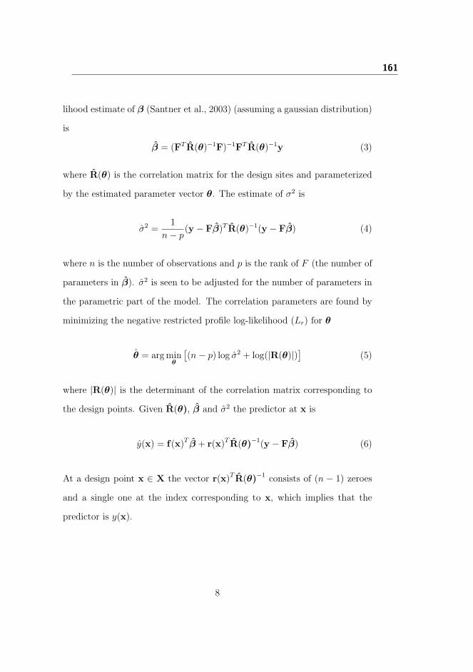
The correlation function is parameterized by a set of parameters θ as describedin (4.2). Given θ, the restricted maximum likelihood estimate of β (Santneret al., 2003) (assuming a gaussian distribution) is
β = (FT R(θ)−1F)−1FT R(θ)−1y (4.7)
where R(θ) is the correlation matrix for the design sites and parameterized bythe parameter vector θ. The estimate of σ2 is
σ2 =1
n− p (y − Fβ)T R(θ)−1(y − Fβ) (4.8)
where n is the number of observations and p is the rank of F (the numberof parameters in β). The correlation parameters are found by minimizing thenegative restricted profile log-likelihood (Lr) for θ
θ = arg minθ
[(n− p) log σ2 + log(|R(θ)|)
](4.9)
where |R(θ)| is the determinant of the correlation matrix corresponding to thedesign points. σ and β are functions of R−1 (equation (4.7) and (4.8)); thatis, inverting the correlation matrix for the design sites is required in order toevaluate the likelihood function. This inversion is a computational expensivetask since it takes O(n3) operations. Moreover, the likelihood function may beflat around the optimum, which implies that the search for the optimum maybecome slow (Lophaven et al., 2002a, Li and Sudjianto, 2005). These aspectsare dealt with in the Matlab toolbox DACE by Lophaven et al. (2002b).
Given R, β and σ2 the predictor at x is
y(x) = f(x)T β + r(x)T R−1(y − Fβ) (4.10)
At a design point, x ∈ X, the vector r(x)T R−1 consists of (n − 1) zeroes anda single one at the index corresponding to x, which implies that the predictorbecomes y(x) and thus interpolates the data at the design points. The interpo-lation property is one of the main advantages of using Kriging for deterministiccomputer models.
28 Output analysis
An example of the Kriging predictor is shown in Figure 4.1. It can be seen thatthe interpolator is improving as more design points are added, i.e., the differencebetween the interpolator and the true function is not visible for n = 10 designpoints (Figure 4.1(d)). The performance of the predictor can be measured bythe accuracy, 1/(1 + RMSE), where RMSE is the root mean square predictionerror over a set of test sites. The accuracy is in Figure 4.1 seen to increase as thenumber of design points is increasing. Likewise the correlation between pointsis seen to increase (θ is decreasing) as more design points are included. It canbe seen that the interpolator is able to fit a quite wiggly curve using only twoparameters: β and θ.
Figure 4.1: Illustration of Kriging predictor for 4-10 points. Solid black linescorrespond to the true function, dashed red lines are the Krigingpredictors and ”o” corresponds to the design points. The underlyingsignal is y = cos(6.8πx/2) + 6x
4.2 Regression models 29
4.2 Regression models
If the output of the computer model is stochastic, an interpolator such as theKriging model may not be the best predictor (see for example Figure 1.3(b)).Instead regression methods from physical experimentation can be applied. How-ever, one difference is that in simulation the random error is usually controlledthrough the seed to the random number generator, which implies that the ob-servations may not be independent. In such cases, e.g., generalized least squaresmethods can be used (Kleijnen, 2008). In this thesis we however only considerexperiments with the seed either kept fixed (deterministic simulation) or chosenrandomly for each run (stochastic simulation).
In the following we consider the most general simulation model, which is stochas-tic and has controllable and uncontrollable factors. Let xci be the ith controllablefactor setting, xuj the jth uncontrollable factor setting and sijk the seed in theijkth run. Moreover, we focus on modeling the variation coming from the un-controllable factors and the seed, i.e., consider the combinations of the settingsof the controllable factors as a single categorical variable to simplify the analysisand focus on the uncontrollable factors.
A simple model for stochastic simulation is the general linear model, i.e., themodel
y(xci , xuj , sijk) = βi + εijk (4.11)
where βi is the parameter for the ith controllable factor setting and εijk ∼N(0, σ2). In equation (4.11) the variation due to the uncontrollable factors isignored and pooled into a single variance component together with the variationdue to the seed. The variation coming from changes in the uncontrollable factorscan be estimated by fitting a linear mixed effects model, which is given as
y(xci , xuj , sijk) = βi + Uj + Sijk (4.12)
In the linear mixed effects model the variation due to the uncontrollable factorsis captured in Uj ∼ N(0, σ2
U ), whereas the variation due to the seed is capturedin Sijk ∼ N(0, σ2
S). Uj and Sijk are assumed to be independent, which impliesthat the variance of a single test/run can be written as σ2 = σ2
U + σ2S .
In Paper C a generalized additive model (Hastie and Tibshirani, 1990, Wood,2006) is applied to the output from a top-down and a crossed experiment onthe simulation model for the surgical unit. The model is also used in Papers Dand E as an extension to the linear and linear mixed effects models. The gen-eralized additive model (GAM) is given as a function of both controllable and
30 Output analysis
(a) Linear model (b) Linear mixed effectsmodel
(c) GAM model
Figure 4.2: Illustration of models for output from stochastic simulation modelwith controllable and uncontrollable factors
uncontrollable factors
y(xci , xuj , sk) = βi +
m∑
l=1
fl(xu(l)j ) + Sijk (4.13)
with xu(l)j being the jth setting for the lth uncontrollable factor and Sijk ∼
N(0, σ2S) the residual or seed term. fl is a spline based smooth function with
the smoothness determined by a penalty term. By estimating the functionalrelationship between the uncontrollable factors and the outcome, the uncontrol-lable factors that are needed to be tightly controlled may be identified. Butmore importantly interactions between controllable and uncontrollable factorsmay also be estimated by fitting different smooth functions depending on thesettings of the controllable factors. The interactions between controllable anduncontrollable factors may be used to put the system in a more robust operatingmode as suggested by Bursztyn and Steinberg (2006) and Myers et al. (2009).The estimation of the β’s and the smooth functions can for example be donewith the R-library (R Development Core Team, 2007) provided by Wood (2006).
A graphical overview of the three models is given in Figure 4.2, which showsthat the models have increasingly more structure for the uncontrollable factors.The models may also be expanded by putting more structure in the controllablefactor part, e.g., including low order polynomials to account for the effects of thecontrollable factors. In this thesis we, however, primarily focus on describing thevariations in the uncontrollable factors. For all three models generalized versionsexist such that, e.g., binomial and count data can be fitted. The generalizedversions are considered in Paper D for estimating the risk of putting the surgicalunit in a worse operating mode compared to the current setting.
4.3 Example: Optimization using a meta-model 31
4.3 Example: Optimization using a meta-model
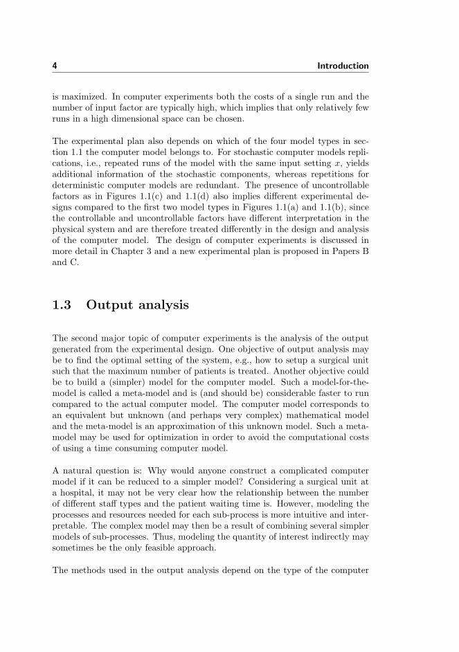
If the computer or simulation model is too expensive to use directly for opti-mization a meta-model can be used as a replacement of the expensive model.Optimization can, e.g., be done in the following four stages
1. run initial design on expensive computer model
2. fit a meta-model based on the observations from the initial design
3. optimize the system using the meta-model
4. validate the optimal setting by running a small number of control runs onthe computer model (and possibly return to the second step after addingmore observations if optimum is not reached)
Using the meta-model not only speeds up the optimization but may also in-crease the understanding of the complex computer model if the simpler meta-model has a more explicit relationship between the input factors and the output(provided that the meta-model is an adequate description). However, using ameta-model assumes that the optimum is within the design region (local opti-mization), whereas the response surface methodology is generally preferred forglobal optimization (see for example Myers et al., 2009).
We now illustrate optimization using a meta-model by a small example with aknown function, which is given as y(x1, x2) = (10x1 − 6) exp[−(10x1 − 6)2 −(10x2−6)2] for (x1, x2) ∈ [0, 1]2. A contour plot of the true function is shown inFigure 4.3, which shows that the function is mostly flat and has its maximumand minimum in the same proximity. The objective of the optimization is tofind the minimum of the function y(x∗) = y(x∗1, x
∗2) by using a meta-model for
the optimization task. In this example a Kriging model is used, since the outputis deterministic.
First an initial maxmin LHD(10,2) is constructed and then the computer modelrun for these ten settings. This gives a set of observations y1, . . . , y10 at thedesign sites (x1
1, x12), . . . , (x10
1 , x102 ) for which a Kriging model is fitted. Opti-
mization can then be done by evaluating the Kriging predictor over a fine gridof say 10.000 points or by using standard optimization software, e.g., optim inR (R Development Core Team, 2007). This gives the estimated minimum x∗
with the predicted value y(x∗).
The estimated minimum, x∗, based on the initial ten points is marked by ”1” inFigure 4.3(a). It can be seen that x∗ is in the neighborhood of the true minimum,
32 Output analysis
x1
x 2
0.0
0.2
0.4
0.6
0.8
1.0
0.0 0.2 0.4 0.6 0.8 1.0
1
●
●
●
●
●
●
●
●
●
●
True function
0.0 0.2 0.4 0.6 0.8 1.0
1
●
●
●
●
●
●
●
●
●
●
Kriging
−0.4
−0.2
0.0
0.2
0.4
(a) 10 initial data points (maxmin LHD)
x1
x 2
0.0
0.2
0.4
0.6
0.8
1.0
0.0 0.2 0.4 0.6 0.8 1.0
12
34
●
●
●
●
●
●
●
●
●
●
●
●
●
●●
True function
0.0 0.2 0.4 0.6 0.8 1.0
12
34
●
●
●
●
●
●
●
●
●
●
●
●
●
●●
Kriging
−0.4
−0.2
0.0
0.2
0.4
(b) After 15 additional data points
Figure 4.3: Optimizing computer model by using a meta-model. a) shows theinitial model to the right and the true function to the left. Theestimated optimum is marked with ”1” and the data points with”O”. b) shows the model after three iterations with the estimatedoptimums marked by connected lines.
4.3 Example: Optimization using a meta-model 33
but still not entirely correct. The relative difference between y(x∗) and y(x∗)(the difference between the true function value at the estimated minimum andthe estimated function value at the estimated minimum) is more than 50 %(Figure 4.4(a)).
To improve the estimated minimum new points are added and evaluated bythe true function and the Kriging model and x∗ are updated until the relativedifference between y(x∗) and y(x∗) is under 1 %. In this example we add fournew points around x∗ and reuse the already calculated value at the estimatedminimum (calculated for the evaluation of the estimated minimum). It canbe seen from Figure 4.4 that after 15 additional points the difference betweenthe estimated and true minimum is small in both location and function value.Actually the estimated optimums are close in location after 10 additional points,but the predicted value is not. If the computer code is very time consuming,this method may give huge savings in computing time, since the Kriging modelis very cheap to evaluate. This is also utilized by Dellino et al. (2009) to findrobust solutions in simulation by using methods inspired by Taguchi (Taguchi,1987).
34 Output analysis
10 15 20 25
0.01
0.02
0.05
0.10
0.20
0.50
Number of points
Rel
ativ
e di
ffere
nce
(a) Relatively difference between y(x∗) and y(x∗)
10 15 20 25
0.00
00.
002
0.00
40.
006
0.00
80.
010
0.01
2
Number of points
Dis
tanc
e to
true
opt
imum
(b) Distance to true minimum
Figure 4.4: Improvement in Kriging estimator for the minimum of the func-tion considered in Figure 4.3 in terms of function value 4.4(a) andlocation 4.4(b)
Chapter 5
Summary of papers
5.1 Paper A
Conditional Value at Risk as a Measure for Waiting Time in Simula-tions of Hospital Units
The topic of Paper A is comparison of statistics describing waiting time distribu-tions. In health care applications patient waiting time is a frequently occurringmeasure of quality. The objective is therefore to summarize a sample of wait-ing times, T = t1, . . . , tN , such that certain properties are highlighted. Thebackground of the paper is the simulation model in section 2.2 for which reduc-ing long waiting times for the patients is an important performance parameter.Avoiding or reducing long waiting times is important since according to Bielenand Demoulin (2007) patient satisfaction decreases as the waiting time increases.
Several statistics for samples of waiting times such as the average and maximumwaiting time are used in the literature. In Paper A we propose Conditional Valueof Risk (CVaR) (Kibzun and Kuznetsov, 2003, 2006) as a measure of the extentof long waiting times. CVaR originates from economics where it is used in, e.g.,portfolio management as a measure of risk. For waiting times it becomes ameasure of the risk of long waiting times, which is an important parameter interms of patient satisfaction (Bielen and Demoulin, 2007). Often waiting time
36 Summary of papers
distributions are right skewed consisting of mainly short waiting times, but mayalso have long tails corresponding to the less frequently occurring long waitingtimes.
The average waiting time taken over all patients corresponds to disregard thedistribution of the waiting times and only focus on the overall waiting time. Thisis in economics known to be a risk neutral strategy, i.e., it only considers theexpected loss and not the risk of big losses. Another measure is the maximumwaiting time, which is seen to belong to the other extreme where the shape ofthe distribution once again is ignored but now only the longest waiting timeis used. Using the maximum is in economics known as a risk averse strategy.The maximum waiting time is also a problematic statistic, since it is a measureof an extreme (it relies on a single observation); that is, the uncertainty of themaximum waiting time is high and hence may require a large sample and manyreplications to estimate properly. Moreover, it may be a too restrictive strategyand may also not represent the performance of the system, e.g., be an extremelyrare observation in an otherwise well performing system.
In Paper A we propose CVaR as a compromise between these two extremes.CVaR is the average of the (1− α)100% longest waiting times and is given as
CV aRα(T ) =1
1− α
[(iαN− α
)tiα +
N∑
i=iα+1
tiN
](5.1)
where α is the level of risk aversion, t1 ≤ t2 ≤ · · · ≤ tN are the ordered waitingtimes, iα is the index satisfying iα
N ≥ α > iα−1N (the α-percentile) and N is the
sample size. It can be seen that CV aR0(T ) = T (the average waiting time)and limα→1 CV aRα(T ) = maxi=1,...,N ti (the maximum waiting time). CVaRcan therefore be seen as a compromise between the average and the maximumwaiting time and α determines the relative importance of the longest waitingtimes or the level of risk aversion. A related measure is the Value at Riskwaiting time (VaR), which is given as V aR = tiα . It is however generally notrecommended, since it is not sensitive to the shape of the distribution of the(1− α)100% longest waiting times.
The benefits of using CVaR are illustrated by a simulation model of an ortho-pedic surgical unit. The model was developed in collaboration with GentofteUniversity Hospital, Copenhagen. The paper consists of two examples; in thefirst example the porter resource is varied from one to four porters and in thesecond example the volume of the elective patients is increased by 7, 14 and29 % while the number of porters is kept constant at four. The examples illus-trate that the average waiting time is not always the best statistic since it mayoverlook important shifts in the tail of the waiting time distribution. Figure 5.1and 5.2 show that the absolute changes in CVaR are larger compared to the
5.1 Paper A 37
Waiting time (minutes)
Density
0.000
0.005
0.010
0.015
0.020
0.025
20 40 60 80 100 120
0
0.001
0.002
0.003
0.004
70 80 90 100
4 porters 4 porters a 4 porters b 4 porters c
Density
0.000
0.005
0.010
0.015
0.020
0.025
20 40 60 80 100 120
0
0.001
0.002
0.003
0.004
70 80 90 100
1 porter 2 porters 3 porters 4 porters
Figure 5.1: Estimated densities for seven different scenarios: 1-4 porters (top)and 4 porters with 7, 14 and 29 % more elective patients (bot-tom). The average waiting times are marked with solid verticallines, whereas the CVaR waiting times are marked with dashed ver-tical lines.
WT
Porters
30
31
32
33
34
1 2 3 4 4a 4b 4c
●
●● ●
● ●●
●●
●
●●
●
● ●
●
●●
MWT
Porters
100
120
140
160
1 2 3 4 4a 4b 4c
●
● ● ● ● ● ●
●●
●●
●
●
●
●
●
●
●
●
TT
Porters
1600
1700
1800
1900
2000
2100
1 2 3 4 4a 4b 4c
● ● ● ●
●
●
●
●●●●●
●●
●
●
EOUT
Porters
10
15
20
1 2 3 4 4a 4b 4c
●● ● ●
●●
●
●
●
●
●●
●
CVaR
Porters
70
75
80
1 2 3 4 4a 4b 4c
●
●● ●
● ●●
●●
●
VaR
Porters
58
60
62
64
66
68
1 2 3 4 4a 4b 4c
●
● ● ●●
●●
●●
Figure 5.2: Comparison of six different performance measures for seven differentscenarios: 1-4 porters and 4 porters with 7 % (4a), 14 % (4b) and29 % (4c) more elective patients. WT is the average waiting time,MWT is the maximum waiting time, TT is the total throughput,EOUT the percentage of elective patients treated outside regularhours, CV aR is the CVaR waiting time and V aR is the VaR waitingtime.
38 Summary of papers
average waiting time, since CVaR is more sensitive to changes in the tail of thewaiting time distribution.
Figure 5.2 furthermore shows that using the maximum waiting time may beproblematic due to the uncertainty of this statistic; that is, the maximum wait-ing time is close to being the same regardless the number of porters and electivepatient volume. The example shows that the compromise between the averagewaiting time and the maximum waiting time given by the CVaR waiting timeis a reliable measure for measuring the extent of long waiting time.
Dellino et al. (2009) use constrained optimization, i.e., they optimize the meangiven a standard deviation constraint. This leads to the so-called Pareto-optimalfrontier, i.e., a curve showing the relationship between the risk (standard de-viation) and the profit (the mean). They fit separate Kriging models for themean and for the standard deviation and use bootstrapping to estimate regionsof confidence for the mean and standard deviation given a specific constraint.As also mentioned by the authors, CVaR may be used as replacement of themean-variance technique.
5.2 Paper B
Designing Simulation Experiments with Controllable and Uncontrol-lable Factors
In Paper B design of simulation experiments with two types of factors (con-trollable and uncontrollable) is considered. The two factor types have differentinterpretation in the physical system and hence need to be treated differently;that is, the system is optimized in the controllable factors such that the settingis optimal disregarding the settings of the uncontrollable factors. The exper-imental design is therefore required to be run under various settings of theuncontrollable factors for each combination of the controllable factors.
Models with controllable and uncontrollable factors are often analyzed using acrossed design (Kleijnen, 2008). This implies that the same combinations of set-tings for the uncontrollable factors are used for all combinations of the control-lable factor settings (whole plots) and hence that the uncontrollable factor spaceis sparsely covered due to the replications as discussed in section 3.3. It couldtherefore be argued that using different settings of the uncontrollable factors foreach whole plot is a better way of choosing the settings of the uncontrollablefactors. For nc whole plots this gives nc as many different uncontrollable factorscombinations, i.e., a higher coverage of the uncontrollable factor space.
5.2 Paper B 39
The main challenge in designing such an experimental plan is to make the sub-designs for the uncontrollable factors similar from one whole plot to the nextwhile ensuring that the overall design is uniform. In Paper B this is achievedin two different ways. The first strategy has a bottom-up structure and thedesign is constructed from nu regions each consisting of nc space-filling points(see Figure 5.3).
0.0 0.2 0.4 0.6 0.8 1.0
0.0
0.2
0.4
0.6
0.8
1.0
x1
x 2
●
●
●
●
●
●
●
●
●
●
●
●
●
●
●
●
●●
●
●
Figure 5.3: Illustration of bottom-up design with four subregions
The whole plots are then assigned one design point from each of the nu re-gions such that all points are assigned. However, the bottom-up strategy doesnot guarantee the uniformity of the combined design, which can be seen fromFigure 5.4. The best bottom-up design with 200 runs (five controllable factorsettings each with 40 uncontrollable factor settings) for two uncontrollable fac-tors is seen to have a WD-value approximately five times higher than an uniformdesign generated directly.
Instead we propose a second strategy, which has more of a top-down structurewhere the overall design is constructed first to guarantee the overall uniformity(see section 3.4). The overall design is then split into subdesigns one for eachwhole plot. The subdesigns are generated by splitting the N = nunc pointsinto nu subgroups of nc points and then assigning each whole plot one pointfrom each subgroup. The assignment of points can be done in many ways andthe WD-values of the subdesigns are used as criteria for the best assignment,we choose the assignment where the maximum WD-value of the subdesigns
40 Summary of papers
●
●
● ●●
●
●
●
●●
●●
●●
●●
●●
● ●
0.0 0.5 1.0 1.5 2.0
12
510
2050
100
Ratio of minimum distance
Nor
mal
ized
WD
●
●
●
●●
●
●
●
●
●
●
●
●
●
●
●
●
●
●
●
Uniform subdesignMaximin subdesign
Maximin full design
Figure 5.4: Uniformity of combined design with bottom-up strategy
is lowest. In Paper C the top-down design is considered in more detail andcompared to the crossed design using the simulation model from section 2.2.
The main contribution in Paper B is the development of an experimental plangiving a high coverage in the uncontrollable factor space for simulation modelshaving both controllable and uncontrollable factors. In paper C we show thatthe higher coverage leads to a better understanding of the uncontrollable factors.
5.3 Paper C
Designing simulation experiments with controllable and uncontrol-lable factors for applications in health care
In Paper C we reconsider the proposed experimental design in Paper B. Thebenefit of using the top-down design is illustrated by the simulation model de-scribed in section 2.2 (see also Paper 5.1). The top-down design is comparedwith the crossed design (see equation 3.8), which is the most commonly useddesign for simulation experiments with controllable and uncontrollable factors.The output is analyzed with generalized additive models (Hastie and Tibshirani,1990, Wood, 2006) for both of the considered experiments (see section 4.2).
5.3 Paper C 41
The model output is modeled by the GAM model, i.e., a flexible regressionmethod. In the paper it is shown that the top-down design identifies importantinteractions between the controllable and uncontrollable factors, which in theexample is not identified using the crossed design (see Figure 5.5). These in-teractions are important, since they may be used to put the system in a robustoperating mode.
Recovery bed occupancy(% increase)
Par
tial e
ffect
on
CV
aR (
min
utes
)
6 Recovery beds
−2
0
2
4
−20 −2 15 32 50
Top−down design
Recovery bed occupancy(% increase)
Par
tial e
ffect
on
CV
aR (
min
utes
)
8 Recovery beds
−2
0
2
4
−20 −2 15 32 50Anesthesiologists occupancy
(% increase)
Par
tial e
ffect
on
CV
aR (
min
utes
)
2 Anesthesiologists
−2
0
2
4
−20 −2 15 32 50Anesthesiologists occupancy
(% increase)
Par
tial e
ffect
on
CV
aR (
min
utes
)
3 Anesthesiologists
−2
0
2
4
−20 −2 15 32 50
Recovery bed occupancy(% increase)
Par
tial e
ffect
on
CV
aR (
min
utes
)
6 Recovery beds
−4
−2
0
2
4
−20 −2 15 32 50
Crossed design
Recovery bed occupancy(% increase)
Par
tial e
ffect
on
CV
aR (
min
utes
)
8 Recovery beds
−4
−2
0
2
4
−20 −2 15 32 50Anesthesiologists occupancy
(% increase)
Par
tial e
ffect
on
CV
aR (
min
utes
)
2 Anesthesiologists
−30
−20
−10
0
10
20
30
−20 −2 15 32 50Anesthesiologists occupancy
(% increase)
Par
tial e
ffect
on
CV
aR (
min
utes
)
3 Anesthesiologists
−30
−20
−10
0
10
20
30
−20 −2 15 32 50
Figure 5.5: Interactions between controllable and uncontrollable factors
The top-down design may also be used as a method for generating a sequentialsampling scheme in the following manner: disregard the controllable/uncontrollablesetup, instead we consider the top-down design as nc batches of runs, which arerun sequentially one batch at the time. This may give a faster completion ofthe experiment if not all batches are needed. However, this only works in thesimple case with only one type of factors in which the controllable factors set-tings correspond to batches and the uncontrollable factors to the factors of themodel. Kleijnen and van Beers (2004) also consider sequential sampling usingKriging as a meta-model, which is extended in van Beers and Kleijnen (2008)who consider sequential sampling for random simulation. Sequential samplingfits very well with simulation, since the simulation experiments are run sequen-tially. Strategies for generating the next sampling point and/or stopping theprocedure can therefore be implemented between two runs or between batchesof runs.
A modification of the top-down design is to consider a different distribution of
42 Summary of papers
the points, i.e., instead of an uniform distribution in each dimension, it may bemore relevant to spread the points out corresponding to a gaussian distribution.In such a design the emphasis is put on the center of the gaussian distributioncorresponding to that certain regions are of greater importance than others, e.g.,a-priori knowledge lead us to believe that the optimum or the function is highlyvariable in these regions. The uniform design spread the points evenly on eachfactor, which can be transformed to a gaussian distribution in the following way
1. Construct a top-down design withN = ncnu runs and p uncontrollable fac-tors and denote the settings of i’th uncontrollable factor xi = [xi1, . . . , x
iN ],
which all belong to the interval [0, 1]
2. for the ith uncontrollable factor define a mean ui and a standard deviationσi corresponding to the area of interest
3. transform xi by the transformation xi = [Φ−1(xi1), . . . ,Φ−1(xiN )] whereΦ−1() is the quantile function for the standard gaussian distribution
4. transform xi to xiG = µi + σixi
This gives uncontrollable factor settings that independently of each other aregaussian with mean µi and standard deviation σi. Figure 5.6 illustrates themethod for N = 4× 25 runs for one uncontrollable factor, which shows that thesubdesigns can be assumed to be gaussian (p-values for shapiro-wilk’s test fornormality are p > 0.93 for the subdesigns and p ≈ 1 for the combined design).This procedure can be generalized to other distributions by replacing Φ−1()with the relevant quantile functions in step 3 and skipping or modifying step 4.
5.4 Papers D and E
Analysis of Computer Experiments with Multiple Noise Sources (Eu-ropean Network for Business and Industrial Statistics)
Paper D illustrates several modeling techniques for the output from simulatingthe surgical unit from section 2.2. The paper was expanded and modified to thejournal article in Paper E and is hence covered by the summary for Paper E
Analysis of Computer Experiments with Multiple Noise Sources
Paper E is an extension of Paper D for the ”ENBIS8” special issue in QualityReliability Engineering International. The modeling techniques in Paper D are
5.4 Papers D and E 43
xG
Den
sity
0.0
0.1
0.2
0.3
−4 −2 0 2 4
● ●●●●●●●●●●●●●●●●●●●●●● ● ●
Whole plot 1
● ● ●●●●●●●●●●●●●●●●●●●●●● ●
Whole plot 2
● ●●●●●●●●●●●●●●●●●●●●●● ● ●
Whole plot 3
−4 −2 0 2 4
0.0
0.1
0.2
0.3
● ● ●●●●●●●●●●●●●●●●●●●●● ● ●
Whole plot 4
Figure 5.6: Transformation of uncontrollable factor settings in a top-down de-sign to gaussian distributions
in this paper also evaluated on a simpler example in which the output functionis known.
In Paper E we consider the M/M/m-queuing system to illustrate the methodsapplied on the more complicated model from section 2.2, since the M/M/m-queuing system is a well-known system and is expected to behave similarlyto the simulation model. The M/M/m-queuing system has a vast literatureand possesses many nice properties including that the expected waiting timeis known (see section 2.3). This implies that the modeling techniques can becompared with the true underlying signal.
The simulation models considered are both influenced by uncontrollable factorsand stochastic sources, which is dealt with in three different manners as de-scribed in section 4.2. The paper shows that the variation in the output can besplit up in two sources by techniques known from physical experimentation. Ina linear mixed effects model a variance component for the variation coming fromchanges in the settings of the uncontrollable factors and an estimator for thevariance coming from changes in the seed (the random error) can be estimated.Moreover, the variation coming from changes in the setting of the uncontrollablefactors can be analyzed and interpreted by means of generalized additive models(GAMs).
For the case-study two scenarios are considered: 1) the current setup and 2)20 new settings of the controllable factor. The 20 new settings were found in
44 Summary of papers
Acute interarrival(a)
CV
aR
6570
75
−1 −0.5 0 0.5 1
1.00
2.54
Porter occupancy(b)
CV
aR
6570
75
−1 −0.5 0 0.5 1
0.52
1.04
Anesthesiologists occupancy
(c)
CV
aR
6570
75
−1 −0.5 0 0.5 1
3.93
5.41
Recovery bed occupancy
(d)
CV
aR
6570
75
−1 −0.5 0 0.5 1
0.61
5.79
Figure 5.7: Estimated effects of the uncontrollable factors. Top curves are thereference setting and the bottom curves the new settings
a pilot study and were chosen such that the CVaR waiting time is expected tobe low while maintaining the same total throughput and percentage of electivepatients treated outside regular hours (EOUT). The analysis shows that withthe current setting the output varies more both due to the uncontrollable factorsettings and the seed, i.e., it is less robust compared to the new settings. Thiscan also be seen from Figure 5.7, which shows that the estimated effects of theuncontrollable factors are flatter for the new settings compared to the currentsetup. Moreover, the estimated CVaR waiting time is 6.5 minutes shorter withthe new settings, which shows that the improvement is significant. It was alsoshown that the methods worked well on the M/M/m-queuing system, i.e., wasable to estimate the true function accurately.
The GAM framework also provides methods for handling binary and count out-comes, which in Paper E was used to estimate the likelihood that a new settingwould perform at least as good as the current settings. The analysis highlightedthree different settings of the controllable factors that had both higher through-puts, smaller percentages of elective patients treated outside regular hours andshorter CVaR waiting times compared to the current setting. All three settingssuggested changing the number of operating days (for elective surgery) from fiveto four, i.e., fewer but longer days.
5.5 Paper F 45
5.5 Paper F
2-stage approach for Kriging for simulation experiments with quan-titative and qualitative factors
The topic of Paper F is Kriging for simulation models with quantitative andqualitative factors. The simulation model in section 2.2 is used for illustrationof the extension of the Kriging interpolator after being put in a deterministicoperating mode. The controllable factors are now thought of as being qualitative(they are ordinal having a few levels only), whereas the uncontrollable factorscorrespond to the quantitative factors. In section 4.1 the basic Kriging model isdescribed and the following is based on those definitions. To ease the notationwe denote one setting of the qualitative factors a whole plot, which reflects thestructure of the top-down experiment (Dehlendorff et al., 2011) applied to thesimulation model.
The usual correlation function given in equation (4.2) is now modified by in-cluding an extra term depending on the whole plots of the observations, i.e.,R(xij , xkl) = R(xij , xkl) · (I(i = k) + I(i 6= k)αik), where xij is the ith wholeplot and jth observation. Five different correlation structures are considered
1. αik = θc: correlations between observations from different whole plots arereduced by a constant quantity
2. αik = g(µi, σi, µk, σk): correlations between observations from differentwhole plots are reduced by a quantity depending on the sample meansand standard deviations of whole plot i and k
3. 2-stage procedure (described below)
4. αik = exp
(−
dz∑q=1
θzqI(zqi 6= zqk)
)where zqi is the level of the qth qualita-
tive factor for the ith observation (see Hung et al. (2009))
5. αik is parameterized by a hypersphere parameterization as proposed by Zhouet al. (2010)
In the 2-stage procedure we first fit a Kriging model for each whole plot in thequantitative factors
Yi(xij) = µi + Zi(xij) i = 1, . . . ,m (5.2)
New design sites are then generated by adding the correlation parameters ofmodel i to all observations from whole plot i, i.e., the design sites becomes
46 Summary of papers
X =[X
[CT
1 ⊗ 11×q1 . . . CTm ⊗ 11×qm
]T ] where X is the original designsites ordered by whole plot, qi is the number of observations from whole plot iand Ci the correlation parameters for whole plot i. An overall model is thenestimated using y and the new design sites X using the standard Kriging modelin (4.1). This implies that whole plots that have similar correlation structureare defined to be close and therefore correlated. The idea is similar in the mean-variance case, but now Ci = [µi σi]. This structure assumes that whole plotswith the same mean and variance are similar.
The five correlation functions are first evaluated on six test functions, whichshows that the mean-standard deviation and 2-stage procedures give the mostaccurate meta-models. On two realistic examples using the simulation model ofthe surgical unit from section 2.2 the 2-stage procedure outperforms the othercorrelation structures.
One drawback of correlation structures 1-4 is that they can not handle negativecorrelations between whole plots, which is possible with the fifth correlationstructure. However, the flexibility of the fifth correlation structure comes witha price, which is the number of parameter required for correlation between wholeplots. This may result in overfitting for small data sets with many levels of thequalitative factors, which is a likely scenario since computer and simulationmodels tend to be very time consuming and have many factors. In the 2-stageprocedure several Kriging models are fitted, they are however somewhat easierto fit since they are fitted on subsets of the data set in the initial step. Moreover,the total number of correlation parameters in the combined model is twice thenumber of quantitative factors and thus still manageable.
Kriging is a very powerful tool and many new methods within simulation arebased on this method. Stochastic Kriging models as considered by van Beersand Kleijnen (2008) and Ankenman et al. (2010) handle simulation models withstochastic output. Robustness analysis through Kriging is also a relatively newtopic and is for example considered by Dellino et al. (2009), who fit separateKriging models for the mean and standard deviation to estimate the Paretofrontier. The method in this paper is seen to perform well on a simple yetrealistic case-study and hence is an alternative the more complex model by Zhouet al. (2010).
Chapter 6
Discussion
Design and analysis of computer and simulation experiments is a relatively newresearch area. Many challenges are encountered in this area and hence a widerange of methods has been developed. In this thesis contributions in both thedesign and the analysis part of the area are introduced.
The first major contribution is the development of the top-down experiment,which provides an experimental plan with a better coverage of the uncontrollablefactor space compared to the crossed design. Furthermore, application of thedesign on a simulation model showed that the coverage of the uncontrollablefactors improved the understanding of the interactions between controllable anduncontrollable factors. The design is based on uniform designs and one ideafor future research is to consider different underlying designs such as, e.g., themaximin design.
Qian et al. (2009a) and Qian et al. (2009b) consider nested space-filling designs,i.e., a high accuracy experiment is nested within a low accuracy experiment.Qian and Wu (2009) consider sliced space-filling designs based on orthogonaldesigns. The overall design principal of the nested and sliced space-filling designsare seen to be similar to ours, i.e., that the design on both the overall and sublevel is taking to account. In future research it would be interesting to comparethe performance of the top-down design with the nested and sliced designs.Another interesting approach is sequential sampling as considered by Kleijnen
48 Discussion
and van Beers (2004) and van Beers and Kleijnen (2008), who use an adaptivesampling scheme, i.e., the next sampling point is based on a criteria based on theinformation from the already simulated settings. The adaptive procedure mayserve as a benchmark for evaluating the performance of deterministic sequentialsampling based on the top-down design structure as discussed in section 5.3.
The second area of contribution is related to output analysis of simulation mod-els. First the CVaR statistic for waiting time distribution was introduced. Nextmethods for analyzing simulation models with multiple noise sources were con-sidered, and finally a method for Kriging for analyzing computer and simulationmodels with quantitative and qualitative factors was proposed.
The CVaR statistic is a measure originating from finance as a measure of risk.CVaR is relevant if the long waiting times are the primary concern, whereas theaverage waiting time may be more appealing to the management for example ifthe waiting times are related to the staff and not the patients. One drawbackof the CVaR criteria is that the required size of the sample increases as (1− α)decreases. However, it may be seen as a robustness measure, i.e., a low CVaR(close to the mean) indicates a setting that is robust since it implies that therisk of long waiting times is low.
For stochastic simulation several modeling techniques from physical experimen-tation were considered, which were shown to perform well for our case-study.Stochastic Kriging is introduced in a recent paper by Ankenman et al. (2010),who include an extra stochastic element in the usual Kriging model to accountfor the variation from one replicate to the next. Kriging is a very flexible andpowerful meta-model for deterministic simulation and hence the stochastic ver-sion is expected to be useful in applications, in which for example regressionmethods fail. Fitting Kriging models for the average at each setting is an-other method to deal with stochastic simulation as considered by van Beers andKleijnen (2003) and Kleijnen (2008), who apply boot-strapping to estimate theuncertainty related to the replications.
Finally a Kriging model for simulation models with quantitative and qualitativefactor is introduced. The fitting procedure is done in two steps and each stepconsists of ordinary Kriging models with simple correlation structures. Zhouet al. (2010) also consider Kriging for models with quantitative and qualitativefactors and introduces a parameterization that can handle negative correlationbetween different settings of the qualitative factors, which is not handled in ourmethod. For a simple yet realistic case-study it was shown that our methodperformed better than the method by Zhou et al. (2010), it is however expectedthat their method will perform better in cases where negative correlations arepresent. Moreover, if the number of qualitative factors is low and the number ofquantitative factors is high the model by Zhou et al. (2010) uses fewer param-
49
eters compared to our method, whereas with many qualitative factor settingsour method is more efficient in terms of the number of parameters.
Kriging is a popular method and interesting extensions to the Kriging modelmay be analysis of models with multiple outputs and robustness studies asconsidered by Dellino et al. (2009). In this thesis several methods for analysisof the output from our case-study have been considered and robustness is aninteresting extension of our current results. Our results based on regressionmethods indicate that the case-study may be put in a more robust operatingmode, but using methods based on Kriging may expand the knowledge aboutthe uncontrollable factors.
50 Discussion
Paper A
Conditional Value at Risk as aMeasure for Waiting Time inSimulations of Hospital Units
Accepted for publication in Quality Technology and Quantitative Management,Volume 7(2) September 2010, p. 321-336
Conditional Value at Risk as a Measure for
Waiting Time in Simulations of Hospital Units
Christian Dehlendorff1∗ Murat Kulahci1 Søren Merser2
Klaus Kaae Andersen1
1DTU Informatics
Technical University of Denmark
2Clinic of Orthopaedic Surgery
Frederiksberg Hospital
Abstract
The utility of conditional value at risk (CVaR) of a sample of waiting
times as a measure for reducing long waiting times is evaluated with spe-
cial focus on patient waiting times in a hospital. CVaR is the average of the
longest waiting times, i.e. a measure at the tail of the waiting time distribu-
tion. The presented results are based on a discrete event simulation (DES)
model of an orthopedic surgical unit at a university hospital in Denmark. Our
52Conditional Value at Risk as a Measure for Waiting Time in Simulations of
Hospital Units
analysis shows that CVaR offers a highly reliable performance measure. The
measure targets the longest waiting times and these are generally accepted
to be the most problematic from the points of view of both the patients and
the management. Moreover, CVaR can be seen as a compromise between
the well known measures: average waiting time and the maximum waiting
time.
Keywords: Waiting time distribution, Conditional Value at Risk, Simu-
lation, Health Care
2
53
1 Introduction
Simulation studies are widely used in health care applications due to the large
number of uncertainties involved. The complexity of these systems together with
the physical and legal constraints in the actual systems make simulation a very
powerful tool for experimentation to serve as a basis for analytic optimization
methods [4, 9].
Simulation models in health care applications are used both for optimization of
existing facilities [8] and in planning new facilities [18]. Ferrin and McBroom [8]
maximized hospital revenue by process improvements in the emergency depart-
ments. Length of stay (LOS), the number of patients leaving without receiving
care, the percentage of admissions accepted and ambulance diversion hours were
used as outcomes. Miller et al. [18] considered the merging of six emergency de-
partments into one and focused on the average LOS. Their results show that the
LOS can indeed be considerably reduced. They further show that the distribution
of LOS is right-skewed with a long tail. Jun et al. [14] reviewed the health care
simulation literature and concluded that simulation is often used to optimize allo-
cations and as a tool in staff planning. They cited various studies related to patient
scheduling and to staff sizing and planning. They also reported that many studies
use trade-offs between the utilization of doctors, rooms etc. and patients’ waiting
times as outcomes.
Denton et al. [7] studied expected surgical suite waiting time, surgical suite
idle time and total overtime and used a linear trade-off combination of these mea-
3
54Conditional Value at Risk as a Measure for Waiting Time in Simulations of
Hospital Units
sures as a single measure. This linear combination is a cost measure which takes
into account the discomfort of patient waiting time and considers it together with
the lost revenue corresponding to idle surgical suite time and the cost of overtime.
Cayirli and Veral [5] reviewed out-patient scheduling and summarized a num-
ber of possible performance measures related to the quality of such systems. The
time-based measures included the mean, the maximum and the frequency distribu-
tion of the waiting times. Their summary for the suggested performance measures
showed that the majority of studies used mean waiting time, total costs of waiting,
percentage of patient waiting less than a certain threshold, and the variation of
waiting time.
The main objective in this article is to compare Conditional Value at Risk
(CVaR) as a optimization measure for patients’ waiting time with existing mea-
sures and to report on the performance of this new measure based on a specific
case-study of an orthopedic surgical unit. The concept of CVaR is formally in-
troduced in section 3.1 and originates from economics. CVaR was introduced by
Rockafellar and Uryasev [21] as a measure to quantify a distribution of losses;
typically in portfolio scenarios. The measure was introduced as an extension to
Value at Risk (VaR), one of the most commonly used performance measures in
portfolio management. The CVaR criterion focuses on the right tail of the loss
distribution and provides a measure of the expected value of the highest losses.
The CVaR criterion has been used in a wide variety of applications (see for exam-
ple [1], [10] and [27]), but not in the context of our study. The suggested use of
CVaR is for optimization of a given system’s performance in terms of waiting time
4
55
and is relevant in cases where the frequency of long waiting times is the primary
concern.
In this article, a discrete event simulation model of an orthopedic surgical unit
in Copenhagen, Denmark is presented as the case-study. The long term goal for
the simulation study is to minimize the total waiting time, with special focus on
long delays. In the case-study analysis of the uncertainties and behaviour of differ-
ent performance measures including CVaR under various resource and simulation
settings are presented. Moreover, CVaR is compared to other measures using this
model as illustration. The article is structured in the following way: Section 2 de-
scribes the case-study. CVaR is defined in section 3 followed by section 4 where
the performance measure is evaluated by considering the simulation model under
different resource and simulation setups. Finally the key findings are summarized
in section 5.
2 Simulation model
In this section, we present our case-study for evaluating the performance of the
CVaR waiting time criterion in the simulation of an orthopaedic surgery unit. The
level of detail of the model is intentionally kept low, since our main objective is
to use it as an illustration of the CVaR measure.
5
56Conditional Value at Risk as a Measure for Waiting Time in Simulations of
Hospital Units
2.1 The surgical unit
As in much of the rest of the world, over the past decade the Danish public health
care system has been subject to increasing demands for efficiency [14]. The sys-
tem is now under considerable pressure for higher throughput in order to reduce
waiting lists. Avoiding or reducing delays in the system is certainly one of the
many options to reach this goal. Furthermore, fewer and/or shorter delays may
also increase patient satisfaction, an issue that is central to today’s quality and
productivity improvement strategies in general.
The case-study is a surgical unit, which is part of an orthopedic department at a
university hospital in Copenhagen, Denmark. The unit undertakes both acute and
elective surgery and performs more than 4,600 operative procedures a year. While
the patients come from various wards throughout the hospital, the main sources of
incoming patients are the four stationary orthopaedic wards or the emergency care
unit. The outpatients treated in outpatient clinics are not considered in this model
but the resources shared between outpatients clinics and the surgical unit are in-
cluded. Also day-case surgery patients with short recovery times are included in
the model.
2.2 Model description
The conceptual model is outlined in Figure 1. It consists of three main modules: 1)
the incoming module with arrival and wards, 2) the surgical unit with preparation
and operating rooms and 3) the recovery. Module 3 is linked back to module 1,
6
57
since the patients return to the wards for final recovery and discharge.
Figure 1: Conceptual model for an orthopedic surgery unit. The 3 modules areseparated by vertical lines and the arrows indicate the patient flow
The simulation model is implemented in ExtendTM version 6 [17] and con-
trolled from a Microsoft Excel spreadsheet with a Visual Basic for application
script. The patient flow is outlined in Figure 2. All patients are either acute or
elective and are admitted to one of the four stationary wards from where the pa-
tients are collected when an operating theater is ready. Patients are then either
sedated, sent to a preparation room and brought to the operating room or brought
directly to the operating room for sedation and preparation. The patients are op-
erated and hereafter attended to by an anesthesiologist before being moved to the
recovery room. As the patients are moved out of the operating room, cleaning and
preparation of the rooms for the next patients are started.
The resource constraints in the system are process related: available surgeons
for the operation, a free recovery bed and an available porter for moving the patient
to the recovery room, etc. These resources are controlled by a central mechanism
7
58Conditional Value at Risk as a Measure for Waiting Time in Simulations of
Hospital Units
Figure 2: Process diagram for patient flow through the system from ward to dis-charge.
controlled by different schedules, e.g. more resources during regular hours. Shar-
ing between different specialties is handled with the resource pools. In our model
the resources include staff and physical facilities such as operating rooms and re-
covery beds. It should be noted that some resources such as surgeons, anesthesiol-
ogists, porters and recovery beds are shared with other departments or procedures
not directly related to the surgical unit.
2.3 Empirical Data
Prior to the simulation study, a simple registration of the time from patients’ ar-
rival at the surgical unit until their departure to the recovery room was done by
the staff for a period of 3 months. The initial data set held no information on sub-
processes, which implied that a more elaborate registration system was needed.
In the new registration system, the nurses at the surgical unit recorded the patient
flow through the unit from the ward to the recovery room, i.e. each subprocess
8
59
was recorded over a period of 1 month.
The new data was validated on the data collected routinely by the staff prior
to the simulation study by comparing the total time spent at the surgical unit
recorded in the two data sets with a Kolmogorov-Smirnoff (K-S) goodness of
fit test [6], which indicated no significant difference. Furthermore, tests for cor-
relation [12, 2] between processes in the new data set indicated that the subpro-
cess durations were statistically uncorrelated indicating that subprocesses could
be modeled individually.
2.4 Validation and verification
The model was inspected graphically by the management of the department to
verify the patient routing and the procedures. Animation was included in the
model to assist and simplify verification during the presentation of the model.
Model validation corresponding to patient volume and waiting time was car-
ried out by comparing the simulation output with the observed data. All validation
was carried out using graphical methods (QQ-plots, density plots and histograms)
and formal statistical tests (K-S and Wilcoxon rank-sum tests [13]) with a signifi-
cance level of 5 %. A more elaborate validation was also carried out correspond-
ing to the scheme outlined by Sargent [22] and although this concluded that the
model was adequate, it is not presented in this article.
The model parameters were calibrated on the individual processes and queu-
ing times, and finally validated on the total duration defined as the time from
the patient leaving the ward to the the time the patient is moved to the recovery
9
60Conditional Value at Risk as a Measure for Waiting Time in Simulations of
Hospital Units
Total duration (minutes)
Den
sity
0.000
0.002
0.004
0.006
0.008
0 100 200 300 400 500
Observed Simulated
Figure 3: Estimated density functions for observed (black solid line) and 100simulation runs (gray dotted lines) for total time at surgical unit
room. Figure 3 shows that the model tends to mimic the system’s overall behav-
ior, which was confirmed with K-S and Wilcoxon tests indicating no statistical
difference. The throughput, mixture of patients and distribution of patients per
day were validated as a part of the tuning and calibration process.
The incoming rate of elective patients per day was shown to fit a discretized
triangular distribution function, which was also validated by a K-S test. The acute
patients were assumed to have exponentially distributed inter-arrival times. K-
S tests indicated that the distribution of acute patients per day and the ratio of
elective to acute patients were modeled adequately. The acute incoming rate was
much more volatile compared to the one for elective patients. The coefficient of
10
61
variation (CV ), which is defined as the standard deviation divided by the mean,
was 2.5 times higher for the acute patients compared to the elective patients. In
both cases the variation in the observed data set was large with CV greater than
90 %.
3 Performance measures
One of the most essential issues in any simulation study is to define sound and
reliable performance measures [19]. Each simulation run is summarized in a set
of measures, which characterizes the overall performance of the system. Often
more than one measure is investigated in order to quantify the objectives of the
study, e.g. avoiding long waiting times while keeping a certain level of patient
throughput. In this paper Conditional Value at Risk is introduced as a waiting
time measure targeting the longest waiting times and compared to other existing
measures.
3.1 Conditional Value at Risk
Conditional Value at Risk is a concept originating from finance as a measure of
risk [21, 15, 16]. For a distribution of waiting times, T , CVaR is defined as the
expected value of the (1−α)-tail of T , i.e. given as
CVaRα(T ) = E[T |T > qα ] (1)
11
62Conditional Value at Risk as a Measure for Waiting Time in Simulations of
Hospital Units
where qα is the α-quantile, where P(T ≤ qα) = α . For a sample of simulated
waiting times, Tx = {tx1, . . . , txN} (obtained from the xth run), the CVaRα(Tx) is
estimated by
CVaRα(Tx) =1
1−α
[(iαN−α
)txiα +
N
∑i=iα+1
txi
N
](2)
with tx1 ≤ tx2 ≤ ·· · ≤ txN , iα is the index satisfying iαN ≥ α > iα−1
N , txiα is the
α-quantile and in economics denoted as the Value at Risk (VaR). VaR is seen
to be indifferent to the shape of the (1−α)-tail, i.e. a given VaR value covers
situations from short (1−α)-tails to long (1−α)-tails. In most applications of
CVaR the estimate is based on the (1−α)100% = 5% longest waiting times and
in the following CVaR is therefore estimated by equation (2) with α = 0.95.
For waiting times the VaR waiting time is the value of the α-quantile of the
total waiting times, e.g. for α = 0.95, 95 % of the patients have a total waiting
time less than or equal to VaR. CVaR is the average of the 5% longest waiting
times, i.e. a measure about the tail of the waiting time distribution. It is seen that
CVaR is at least as large as VaR and that the difference indicates the skewness of
the distribution, hence the two measures are correlated. CVaR is seen to be more
sensitive to samples with very long waiting times compared to VaR. However,
Webby et al. [27] noted that CVaR, as opposed to VaR, is more stable with changes
in the α-value. This can be explained by the fact that CVaR is an average of the
tail, whereas VaR is the quantile defining the tail. The quantile is likely to jump
with a small sample, whereas the average will shrink this effect.
12
63
The rationale for introducing CVaR waiting time measure is that it is a well
known measure of risk in finance. It fits well in an optimization framework with
the objective of minimizing the overall waiting time while controlling the risk of
experiencing very long waiting times. The tail of the waiting time distribution
in these studies is quite important since as shown by Bielen and Demoulin [3],
in terms of patient satisfaction, waiting time influences satisfaction negatively.
That is, longer waiting times decrease patient satisfaction significantly. Using the
average waiting time inherently imply that the distribution of the waiting times
is unimportant as long as the overall waiting time is low. This is, however, not
in accordance with patient satisfaction and quality perception. On the other hand
the maximum waiting time may be a too risk averse measure and could potentially
confound good settings with bad settings since it is based on only the most extreme
observation.
The benefits of using CVaR as performance measure are that it is easy to com-
pute, easy to interpret and targets the long waiting times. As mentioned above,
if the mean waiting time (denoted risk neutral) is used, an increase in the longest
waiting times can be overlooked since a shift in the tail may be averaged out by
the rest of the distribution. On the other hand, using the maximum waiting time
(risk averse) may corrupt the results, since a single long waiting time may be an
outlier in an otherwise well performing setup. CVaR can be seen as a compro-
mise between the average waiting time (α = 0) and the maximum waiting time
(1−1/N < α < 1), with (1−α) reflecting the risk of long waiting times. Hence
a low α corresponds to a high risk of overlooking long waiting times since the
13
64Conditional Value at Risk as a Measure for Waiting Time in Simulations of
Hospital Units
importance of these is low.
3.2 Other measures
Other measures have been suggested in the health care literature, which are dis-
cussed in the following. Tang et al. [26] presented mean residual life, i.e. the
expected residual life time given that a unit has lived a certain amount of time.
In terms of waiting time this is equivalent to the expected residual waiting time
having waited a certain amount of time. Length of additional stay (LAS) is an-
other metric for measuring waiting times, Silber et al. [24] defined it as the re-
maining length of stay (LOS) after the transition point at which the stay becomes
prolonged. A stay may become prolonged at the first time point, x, where the
probability of a total length of stay of x + y is greater than the probability for a
LOS of y from the beginning. The test for the prolonging point is done with the
Hollander-Proschan test [11]. LAS is seen to be the mean residual life at the point
where the stay becomes prolonged. The rationale behind LAS is that if a stay is
prolonged it is more likely to be associated with a complicated case [24].
Both LAS (the MRL at the prolongation point) and MRL are similar to the
CVaR measure. However, CVaR is the expected waiting time of the (1−α)100%
longest waiting times, whereas mean residual life at the α-quantile is the expected
remaining waiting time after having waited txiα minutes. Silber et al. [24] suggest
using the point at which a stay becomes prolonged as the choice for α . This im-
ply that for different setups the corresponding LAS’s (or MRL’s) are the average
residual waiting times for the prolonged stays, i.e. for different α-values. Fur-
14
65
thermore, the scale is different depending on the setting: in one case it may the
residual waiting time after having waited 30 minutes while in another it may be
the residual waiting time after having waited 60 minutes. For LAS and MRL in
general unlike for CVaR the interpretation is seen to be dependent on the distri-
bution. This implies that the scale and interpretation are maintained for different
settings, which makes it suited for use in optimization. Moreover, the distribu-
tion of waiting times may be on time, i.e. no prolongation point is present, which
implies that the LAS concept breaks down.
From a quality point of view the waiting time may be more interesting than the
residual waiting time, since the patient’s perception of the quality of the treatment
is related to his/her total waiting time and not the residual waiting time after hav-
ing already waited for x minutes. In terms of waiting times the length of additional
stay may not be as important as for the length of a hospital stay, since the waiting
time indicates something about the system’s performance and not of the severity
of the operation or complications for the individual patient. Moreover, the waiting
time is the time between activities and hence complicated cases have longer ac-
tivity times and more difficult recovery, which do not influence the waiting time.
Silber et al. use the LAS as an indicator of health care outcomes and the measure
is hence not targeted at evaluating a system’s performance. The LAS framework
does not seem to be well suited for evaluating waiting times, whereas it is highly
relevant for seeking complicated hospital stays.
15
66Conditional Value at Risk as a Measure for Waiting Time in Simulations of
Hospital Units
4 Case Study
This section presents the performance measures by applying them to output from
the simulation model presented in section 2. The measures are initially examined
under the existing setup in terms of the variation from run to run and the sensitivity
to length and number of runs. They are then considered under different resource
settings. The proposed measure, CVaR, is analyzed and compared to other well
known measures presented in section 4.3.
4.1 Simulation setup
The simulation model is run for at least 300,000 minutes (see section 4.4). This
corresponds to 30 weeks with a warm-up period of 10,080 minutes (1 week) for
each run. In each run different performance measures are obtained as described
in section 4.3. These measures are summarized by their minimum, maximum, av-
erage and coefficient of variation (sample standard deviation in % of the average)
across runs.
4.2 Analysis methods
The results from the simulation model are analyzed using statistical test methods.
Wilcoxon two-sample tests [13] are used to compare two samples in terms of their
location. The test is a non-parametric test. Comparing two samples in terms of
their distributions is done with Kolmogorov-Smirnoff two- sample test [6], which
is also a non-parametric method. Here we compare the empirical distributions
16
67
and test whether they can be assumed to be identical. Significance of correlation
coefficients is tested based on Spearman’s rho [12, 2], a non-parametric approach
based on ranks. The main rationale for using non-parametric tests is that they do
not rely on specific distribution assumptions and are robust against outliers. All
data analysis was done in R version 2.7.1 [20].
Densities functions are estimated with the density procedure from the stats-
package and plotted with the densityplot function from the lattice-package
in R [20, 23] using the default values. The defaults are a Gaussian kernel with
a bandwidth, h = 0.9n−1/5 min[σx, IQRx/1.34], where x is the sample, which has
sample standard deviation σx, inter-quartile range IQRx and sample size n (Silver-
man’s rule-of-thumb) [25].
4.3 Performance measures
The main focus of the simulation study is on the waiting times defined as the
time wasted between processes and is measured in minutes. For each patient a
number of waiting times are identified: waiting time before the surgeon talks to
the patient before sedation, waiting time for the anesthesiologist, waiting time
before operating room is ready and waiting time for a porter and a free recovery
bed, etc. The total waiting time for the jth patient in the ith simulation run, ti j,
is estimated as the sum of K sub waiting times, ti jk. The waiting time measures
considered in this article are
• Average waiting time, WT
17
68Conditional Value at Risk as a Measure for Waiting Time in Simulations of
Hospital Units
• Maximum waiting time, MWT
• Conditional Value at Risk, CVaR, waiting time, CVaR(WT )
• Value at Risk, VaR, waiting time VaR(WT )
Additionally total throughput (total number of patients treated, TT ) and percent-
age of elective patients treated outside regular hours, EOUT , are considered.
These measures are included in the simulation study to ensure that the throughput
remains the same and the elective patients are not treated outside regular hours,
hence without creating additional costs due to overtime. The average and maxi-
mum waiting times are frequently used measures to quantify the waiting time [5].
VaR is included to highlight the additional information contained in our main
measure, CVaR, and to illustrate its close relationship to CVaR.
4.4 Run length and sample size analysis
The first example consists of simulations on the system at its current configuration.
Here, the main objective is to examine the performance measures under different
run lengths and numbers of repetitions (runs). Table 1 shows the summary for
three types of simulation runs for the system as it is: 1) 30-weeks simulation
repeated over 100 runs, 2) 30-weeks simulation repeated over 200 runs and 3)
60-weeks simulation repeated over 60 runs.
From the first block in Table 1 it is seen that the total waiting times are highly
skewed with an average WT of around 31 minutes, a 95 % quantile of around 61
and a maximum of 111 minutes. It is seen from the CV column in the first block
18
69
Table 1: Summary for performance measures over runs, e.g. the minimum, maxi-mum, average and CV of total throughput for three types of simulation setups. TheMin-entry for the first row e.g. summarizes the minimumWT of the 100 runs, Maxthe maximum, Mean the average and CV the standard deviation in percent of themean. The units for the waiting time statistics are minutes, the unit for EOUT ispercent and TT is measured in number of patients.
70Conditional Value at Risk as a Measure for Waiting Time in Simulations of
Hospital Units
Number of runs
CV
(%
)
10 20 30 40 50 60 70 80 90 100
0
1
2
3
7
8
9
10
11
12
13
WT MWT TT EOUT CVaR VaR
Figure 4: Coefficient of variation as function of included runs for the 6 perfor-mance measures
in Table 1 that the most varying measure is the MWT (CV = 11.3%) followed by
EOUT (CV = 9.2 %). The remaining four measures are comparable in terms of
coefficient of variation (1.5% ≤CV ≤ 2.5%).
Figure 4 illustrates the evolution of the CV ’s as the number of runs is increased.
It can be seen that all CV ’s are stabilized after 70 runs, however subdivided into the
two groups as described previously. It can also be seen that the two upper curves
take more runs to settle in compared to the bottom four. Clearly the maximum
20
71
Simulation duration (minutes)
CV
(%
)
100000 175000 250000 325000 400000 475000 550000
0
1
2
3
4
5
6
7
8
9
10
11
12
13
14
15 WT MWT TT EOUT CVaR VaR
Figure 5: Coefficients of variation for 60 runs with varying run lengths for the 6performance measures
waiting time is a measure highly dependent on the simulation run, since it is the
most extreme observation in each run. The average waiting time is as expected the
least varying measure, whereas the CVaR and VaR are seen to vary almost equally
much. Figure 4 indicates that the four best performing measures have stabilized
after 30-40 repetitions.
Figure 5 shows that a run-length of 300,000 minutes (30 weeks) seems to
be adequate for obtaining a low CV for 5 out of 6 measures (no significant im-
21
72Conditional Value at Risk as a Measure for Waiting Time in Simulations of
Hospital Units
provements hereafter). EOUT is seen to be improving by more than 2 %-points
from 300,000 minutes to 600,000. Simulating 30 weeks repeated 60 times is a
good trade-off between simulation time and precision for MWT , which leads to
an approximate half width of a 95 % confidence interval for the average of MWT
corresponding to 2.7% of its estimated value. For WT , TT , VaR and CVaR con-
siderably fewer repetitions are needed. In fact Figure 4 suggests that fewer than
20 repetitions will be sufficient.
In the 100 run simulation of 30 weeks each CVaR is significantly correlated
with VaR (as expected), MWT and WT . Moreover, VaR is significantly correlated
with WT , whereas TT is correlated both with EOUT and WT . The correlations
are all positive, which implies that higher throughput is associated with longer
waiting times. The VaR is seen to be uncorrelated with the MWT , whereas CVaR
is. This in fact fits well with the definition of CVaR and VaR. The connection
between CVaR and WT and MWT was shown in section 3.1.
4.5 Sensitivity to Changes in Resource Allocation
The sensitivities of the measures to changes in resource allocation are analyzed by
changing the number of porters at the surgical unit in regular hours. Three porters
are available in regular hours in the current system described in section 4.4. This
number is set to 1, 2 and 4 in the following analysis. The porters are a relatively
less costly resource to adjust than the number of surgeons, nurses and operation
rooms. The expectations are that lowering the number of porters will increase the
waiting times and decrease the throughput or increase the percentage of patients
22
73
being treated outside regular hours. Hence increasing the number of porters may
enable an increase in the incoming flow of patients without increasing the waiting
times if the remaining resources are underutilized in the current setup.
Table 2 summarizes the results from 60 runs of 30 weeks for three different
settings of porters. It can be seen that having 2 or 4 porters are equivalent with
the results for 3 porters in Table 1, whereas having 1 porter clearly increases the
waiting times in terms of the average, CVaR and VaR waiting time. In the top part
of Figure 6 the associated estimated density functions indicate that 2-4 porters lead
to equivalent waiting time distributions, whereas the 1 porter distribution seems
to differ.
With 1 porter it is observed that all measures besides the total throughput are
changed significantly (Wilcoxon two-sample test [13]: p < 0.001) compared to
having 3 porters. The patients wait longer on average (8.56 % increase on av-
erage), have higher maximum waiting times (8.41 % increase on average), more
patients are treated outside regular hours (19.41 % increase on average) and CVaR
and VaR are increased significantly (7.53 % and 6.97 %, respectively). Figure 6
shows that the primary change from 2-4 porters to 1 porter is a heavier tail. This
is reflected in the CVaR in Table 1 and 2, which show that the increase is around
2 times the increase in the average waiting time. The top part of Figure 6 shows
that the estimated density function with 1 porter is flatter around the peak and has
a thicker tail, which increase the CVaR more than WT . The increase by 5 minutes
in CVaR from 3 to 1 porter corresponds to an increase in waiting time for the
approximately 85 patients with the 5 % longest waiting times of 7 hours. In our
23
74Conditional Value at Risk as a Measure for Waiting Time in Simulations of
Hospital Units
Table 2: Summary for performance measures over runs for three different config-urations as in Table 1. The units for the waiting time statistics are minutes, theunit for EOUT is percent and TT is measured in number of patients.
Figure 6: Estimated densities for 1, 2, 3 and 4 porters (top) and 4 porters withdifferent patient load (bottom). Vertical lines correspond to mean waiting time(solid lines) and CVaR value (dashed lines). Porters 4a, 4b, and 4c correspondto 4 porters with 7 %, 14 % and 29 % more elective patients, respectively. Thedashed area in the lower right of each panel is highlighted in the upper right.
simulation study the difference in CVaR is statistical significant, but the practical
importance of the increase may be limited.
Adding an extra porter does not shorten the waiting times (top block in Ta-
ble 2), the situation is comparable with the original 3 porter setting. The perfor-
mance measures were not significantly different. The lowest p-value is obtained
for VaR with a p-value of 0.18. Figure 7 furthermore shows that increasing the
number of elective patients leads to a significantly worse performance compared
to both the 3 and 4 porter situation (for all measures other than MWT ). The bot-
25
76Conditional Value at Risk as a Measure for Waiting Time in Simulations of
Hospital Units
WT
Porters
30
31
32
33
34
1 2 3 4 4a 4b 4c
MWT
Porters
100
120
140
160
1 2 3 4 4a 4b 4c
TT
Porters
1600
1700
1800
1900
2000
2100
1 2 3 4 4a 4b 4c
EOUT
Porters
10
15
20
1 2 3 4 4a 4b 4c
CVaR
Porters
70
75
80
1 2 3 4 4a 4b 4c
VaR
Porters
58
60
62
64
66
68
1 2 3 4 4a 4b 4c
Figure 7: Box plots for comparing performance criteria for different resourcesettings. 4a, 4b, and 4c correspond to 4 porters with 7 %, 14 % and 29 % moreelective patients, respectively.
tom part of Figure 6 indicates that the patients are waiting longer on average as
the incoming rate is increased and that the tail of the waiting time distribution has
the same length (MWT the same) but is heavier (VaR and CVaR increased).
It can be seen that CVaR has a higher absolute increase compared to WT for
the 3 vs. 1 porter comparison, showing that the 5 % longest waiting times are in-
creased the most. For increased patient input MWT does not increase, whereas
CVaR and VaR do. This shows that using the MWT as criterion for judging the
waiting time performance is a poor choice as it may not pick up differences in the
waiting time distribution due the large uncertainty on this measure of the extreme.
Moreover, the MWT does not consider the shape of the waiting time distributions,
26
77
which may differ in the thickness of the tails but have the same MWT . It is seen
that CVaR picks up the change in the distribution of waiting times by using infor-
mation from the whole tail rather than relying on the most extreme observation in
each run.
5 Conclusions
The analysis of simulation studies needs reliable performance measures to answer
the relevant research questions. In this article CVaR is suggested as a measure
of the tail distribution of waiting times for a surgical unit with the objective of
avoiding long waiting times. Our analysis shows that CVaR is a reliable measure
that is specific to the tail. Moreover, CVaR can be seen as a compromise between
the risk neutral average waiting time and the risk averse maximum waiting time.
The results presented in this article show that using the maximum waiting time is
a poor choice since it is highly variable and ignores changes in the shape of the
waiting time distribution.
The average waiting time is not always representative for the waiting times,
since such distributions often are skewed and long waiting times may potentially
be more problematic from the points of view of patients and management. The
VaR criterion is a measure of a quantile in the distribution but is indifferent to
the tail distribution and does not quantify the tail distribution. In terms of quality
management with patient satisfaction as outcome CVaR is highly relevant since
it quantifies the problematic long waiting times. Moreover, the CVaR criteria
27
78Conditional Value at Risk as a Measure for Waiting Time in Simulations of
Hospital Units
is more stable compared to VaR with respect to the chosen α-level since it is a
sample average. It has nice properties as it is easy to compute and interpret and it
is robust. CVaR of the waiting times may therefore be a relevant outcome in many
quality improvement studies within health care with the objective of reducing the
risk of long waiting times.
6 Author biographies
Christian Dehlendorff is a PhD-student in Informatics and Mathematical Model-
ing at the Technical University of Denmark. He has a M.Sc. in Engineering within
data analysis and statistics. His research interests are within design of experiments
and computer experiments.
Murat Kulahci is an Associate Professor in Informatics and Mathematical
Modeling at the Technical University of Denmark. His research interests include
design of experiments, statistical process control, and financial engineering. He is
a member of the American Statistical Association, European Network of Business
and Industrial Statistics (ENBIS), and the Institute of Operations Research and the
Management Sciences.
Søren Merser is a surgeon (MD) at Clinic of Orthopedic Surgery at Frederiks-
berg Hospital, Denmark. He is a member of Danish Orthopedic Society and his
primary research interest is on-line quality control in hospital units.
Klaus K. Andersen is an Associate Professor in Informatics and Mathematical
Modeling at the Technical University of Denmark. He has a PhD in time series
28
79
analysis and his research interests are within design of experiments and statistical
consulting.
References
[1] Alexander, S., Coleman, T. and Li, Y. (2006). Minimizing cvar and var for a
portfolio of derivatives. Journal of Banking and Finance, 30(2), 583–605.
[2] Best, D. and Roberts, D. (1975). Algorithm as 89: The upper tail probabili-
ties of spearman’s rho. Applied Statistics, 24, 377–79.
[3] Bielen, F. and Demoulin, N. (2007). Waiting time influence on the
satisfaction-loyalty relationship in services. Managing Service Quality,
17(2), 174–193.
[4] Brailsford, S. C. (2007). Tutorial: Advances and challenges in healthcare
simulation modelling. Proceedings of the 2007 Winter Simulation Confer-
ence, 1436–1448.
[5] Cayirli, T. and Veral, E. (2004). Outpatient scheduling in health care: a
review of literature. Production and Operations Management, 12(4), 519–
49.
[6] Conover, W. J. (1971). Practical Nonparametric Statistics. New York: John
80Conditional Value at Risk as a Measure for Waiting Time in Simulations of
Hospital Units
[7] Denton, B. T., Rahman, A. S., Nelson, H. and Bailey, A. C. (2006). Simu-
lation of a multiple operationg room surgical suite. Proceedings of the 2006
Winter Simulation Conference, 414–424.
[8] Ferrin, D. M. and McBroom, D. L. (2007). Maximizing hospital financial
impact and emergence department throughput with simulation. Proceedings
of the 2007 Winter Simulation Conference, 1566–1573.
[9] Fone, D., Hollinghurst, S., Temple, M., Round, A., Lester, N., Weightman,
A., Roberts, K., Coyle, E., Bevan, G. and Palmer, S. (2003). Systematic
review of the use and value of computer simulation modelling in population
health and health care delivery. Journal of Public Health Medicine, 25(4),
325–35.
[10] Garca-Gonzlez, J., Parrilla, E. and Mateo, A. (2007). Risk-averse profit-
based optimal scheduling of a hydro-chain in the day-ahead electricity mar-
ket. European Journal of Operational Research, 181(3), 1354–1369.
[11] Hollander, M. and Proschan, F. (1972). Testing whether new is better than
used. The Annals of Mathematical Statistics, 78(4), 1136–1146.
[12] Hollander, M. and Wolfe, D. A. (1973). Nonparametric Statistical Methods.
New York: John Wiley & Sons. Pages 185-94.
[13] Hollander, M. and Wolfe, D. A. (1973). Nonparametric Statistical Methods.
New York: John Wiley & Sons. Pages 27-33 (one-sample), 68-75 (two-
sample).
30
81
[14] Jun, J., Jacobson, S. and Swisher, J. (1999). Application of discrete-event
simulation in health care clinics: a survey. Journal of the Operational Re-
search Society, 50(2), 109–23.
[15] Kibzun, A. and Kuznetsov, E. (2003). Comparison of var and cvar criteria.
Automation and Remote Control, 64(7), 153–164.
[16] Kibzun, A. I. and Kuznetsov, E. A. (2006). Analysis of criteria var and cvar.
Journal of Banking & Finance, 30(2), 779–796.
[17] Krahl, D. (2002). The extend simulation environment. Proceedings of the
2002 Winter Simulation Conference, 205–213.
[18] Miller, M., Ferrin, D., Ashby, M., Flynn, T. and Shahi, N. (2007). Merging
six emergency departments into one: A simulation approach. Proceedings
of the 2007 Winter Simulation Conference, 1574–1578.
[19] Nakayama, M. K. (2006). Output analysis for simulations. Proceedings of
the 2006 Winter Simulation Conference, 36–46.
[20] R Development Core Team (2007). R: A Language and Environment for Sta-
tistical Computing. R Foundation for Statistical Computing, Vienna, Austria.
ISBN 3-900051-07-0.
URL http://www.R-project.org
[21] Rockafellar, R. T. and Uryasev, S. (2002). Conditional value-at-risk for gen-
eral loss distributions. Journal of Banking & Finance, 26, 1443–1471.
31
82Conditional Value at Risk as a Measure for Waiting Time in Simulations of
Hospital Units
[22] Sargent, R. G. (1998). Verification and validation of simulation models.
Proceedings of the 1998 Winter Simulation Conference, 121–130.
[23] Sarkar, D. (2009). lattice: Lattice Graphics. R package version 0.17-22.
URL http://CRAN.R-project.org/package=lattice
[24] Silber, J. H., Rosenbaum, P. R., Koziol, L. F., Sutaria, N., Marsh, R. R. and
Even-Shoshan, O. (1999). Quality and outcomes of care - conditional length
of stay. Health Services Research, 34(12), 349–363.
[25] Silverman, B. W. (1986). Density Estimation. Chapman and Hall. Page 48.
[26] Tang, L., Lu, Y. and Chew, E. (1999). Mean residual life of lifetime distri-
butions. IEEE Transactions on Reliability, 48(1), 73–78.
[27] Webby, R., Adamson, P., Boland, J., Howlett, P., Metcalfe, A. and Pianta-
dosi, J. (2007). The mekong-applications of value at risk (var) and condi-
tional value at risk (cvar) simulation to the benefits, costs and consequences
of water resources development in a large river basin. Ecological Modelling,
201(1), 89–96.
32
83
84Conditional Value at Risk as a Measure for Waiting Time in Simulations of
Hospital Units
Paper B
Designing SimulationExperiments with Controllable
and Uncontrollable Factors
Invited conference paper published in Proceedings of Proceedings of the 2008Winter Simulation Conference, S. J. Mason, R. R. Hill, L. Monch, O. Rose, T.Jefferson, J. W. Fowler eds.
Proceedings of the 2008 Winter Simulation ConferenceS. J. Mason, R. R. Hill, L. Moench, O. Rose, eds.
DESIGNING SIMULATION EXPERIMENTS WITHCONTROLLABLE AND UNCONTROLLABLE FACTORS
Christian DehlendorffMurat Kulahci
Klaus Kaae Andersen
Department of Informatics and Mathematical ModellingTechnical University of Denmark
Bygning 321, Richard Petersens PladsLyngby, DK-2800, DENMARK
ABSTRACT
In this study we propose a new method for de-signing computer experiments inspired by thesplit plot designs used in physical experimen-tation. The basic layout is that each set of con-trollable factor settings corresponds to a wholeplot for which a number of subplots, each cor-responding to one combination of settings ofthe uncontrollable factors, is employed. Thecaveat is a desire that the subplots within eachwhole plot cover the design space uniformly.A further desire is that in the combined de-sign, where all experimental runs are consid-ered at once, the uniformity of the design spacecoverage should be guaranteed. Our proposedmethod allows for a large number of uncon-trollable and controllable settings to be run ina limited number of runs while uniformly cov-ering the design space for the uncontrollablefactors.
1 INTRODUCTION
With the current advances in computing tech-nology, computer and simulation experimentsare increasingly being used to study complexsystems for which physical experimentation isusually not feasible. Our case study involves adiscrete event simulation model of an orthope-
dic surgical unit. The discrete event simulation(DES) model describes the individual patient’sprogress through the system and has been de-veloped in collaboration with medical staff atGentofte University Hospital in Copenhagen.The unit undertakes both acute and electivesurgery and performs more than 4,600 opera-tive procedures a year. While the patients comefrom various wards throughout the hospital, themain sources of incoming patients are the fourorthopedic wards or the emergency care unit.
The simulation model is implemented inExtend version 6 (Krahl 2002) on a WindowsXP platform and controlled from a MicrosoftExcel spreadsheet with a Visual Basic for ap-plication script. The model consists of 3 mainmodules: The wards and arrival, the operatingfacilities, and the recovery and discharge. In-teractionwith thesurroundinghospital is forex-ample modeled with simplified processes usingthe same resources as the processes in the surgi-cal unit (occupying the resources) and with thepatients entering and exiting the model. Oper-ating rooms, recovery beds, wards and staff areincluded in the model. The average run time forsimulating 6 months (with one week of warm-up) operations is around 7 minutes. Typicaloutcomes are waiting times, patient through-put and the amount of overtime.
86Designing Simulation Experiments with Controllable and Uncontrollable
Factors
Dehlendorff, Kulahci and Andersen
The simulation model has two sources ofnoise coming from variations in the uncontrol-lable factors (a.k.a. environmental factors inphysical experimentation) and from changes intheseedcontrolling therandomnumbergenera-tionprocessembedded in thesimulationmodel.The controllable factors are for example thenumber of operating rooms and the numberof surgeons, whereas the uncontrollable fac-tors may include for example the arrival rateof acute patients and the time required to cleanthe operating rooms.
In this type of application, several issuesneed to be considered. First, the controllablefactors tend to be numerous and often discrete.Moreover a single experiment usually takesseveral minutes to run. Therefore a simple ex-haustive method, where all possible combina-tions of the factor settings are considered, isoften computationally infeasible due to the ex-ponentially increasing number of factor com-binations. Furthermore, the settings of the un-controllable factors, e.g. the acute patient ar-rival rate or the duration of surgical procedures,are also of interest and must be determined asthey may influence the outcome of the simula-tions and hence the robustness of the simulationanalysis.
The paper is organized in the followingmanner: Section2 introduces design of com-puter experiments and defines the performancemeasure for the designs. Section3 describesthe proposed design method and contrasts itwith other methods. In section4 opportunitiesfor future research are presented. Finally themain conclusions are summarized in section5.
2 DESIGN OF COMPUTEREXPERIMENTS
2.1 Literature Review
A general discussion on the issues regardingthe design and analysis of computer exper-iments can be found inSacks et al. (1989),
Santner, Williams, and Notz (2003)and Fang, Li, and Sudjianto (2006). Theoutputs from the computer experiments areoften considered to come from a determin-istic computer code. In such experiments,the classical design of experiment meth-ods such as replication is deemed to beredundant as replication of an experiment,for example, yields exactly the same result(see Santner, Williams, and Notz (2003)andFang, Li, and Sudjianto (2006)).
Experiments based on a simulationmodel often involve some stochastic com-ponent; making the output also stochastic.Kleijnen (2008) discusses the design andanalysis of simulation experiments whichtypically have some sort of noise in the output.Therefore these experiments differ from thedeterministic computer experiments. Further-more, a typical simulation application willhave both controllable and uncontrollable (en-vironmental) factors, which should be handleddifferently. In these applications the aim isto manipulate the controllable factors so thatthe system is insensitive (robust) to changesin the uncontrollable factors. As describedby Kleijnen (2008) and Sanchez (2000)thesolution’s robustness needs to be considered inorder to obtain applicable solutions in systemswith uncontrollable factors. That is, a goodsolution needs to perform well over the entirerange of uncontrollable factors.
The original concept of robustnessin physical systems is often attributedto Taguchi (1987). Taguchi’s methods involvean inner array for the controllable factors andan outer array for the uncontrollable factors.In simulation studies,Kleijnen (2008) sug-gests using a crossed design, e.g. combininga central composite design (CCD) for thecontrollable factors and a Latin HypercubeDesign (LHD) for the uncontrollable factors.In a crossed design the same set of subplots isused for each whole plot. However, as we will
87
Dehlendorff, Kulahci and Andersen
show in this study, this may not be the mostefficient way of running such experiments.
2.2 Simulation Model
Our basis is a discrete event simulation modelgeneratingoutput,y = f (xc,xe), for thesettingsfor the sc controllable factors,xc, and the set-tings for these uncontrollable factors,xe. Theobjective is not only to select the settings,x∗c ,such that the solution is robust to changes in theuncontrollable factor settings as described in p.130-134 inKleijnen (2008), but also to under-stand the variation coming from the changes inthe uncontrollable factor settings.
Since little prior knowledge of both con-trollableanduncontrollable factors isavailable,we require that a good design is simultaneouslyuniform over the design space of the control-lable and uncontrollable factors. In the follow-ing, we will assume that the uniform coverageof the design space of the controllable factorsis already achieved and that we are only con-cerned with the uncontrollable factors.
Robustness studies in physical exper-imentation often involve split-plot de-signs (Montgomery 2005). We will thereforeuse similar terminology when robustnessstudies are performed using computer exper-iments. In classic split-plot designs, a set ofexperiments called whole-plots is designed sothat for each whole-plot another set of exper-iments called subplots are run. In robustnessstudies, the settings of the controllable factorsoften constitute the whole-plots, whereas thesettings of the uncontrollable factors constitutethe subplots. In Table1, a whole-plot corre-sponds to a row in which randomly selectedcombinations of settings for the uncontrollablefactors are run. It should be noted that therandomization issue is irrelevant for computerexperiments.
In the proposed method, each whole-plotcorresponds to one combination of settings ofthe controllable factors (a row in Table1), i.e.
a total ofnc whole-plots are needed (nc = 5 inTable1). Each subplot (a column entry in anyrow in Table1) corresponds to a combinationof settings for the uncontrollable factors witha total ofk subplots for each whole-plot. Thusthe overall design consists ofN = nck runs. In acrossed design as proposed byKleijnen (2008)thesek subplots would be the same from onewhole-plot to the next. Therefore there willonly be a total ofk combinations of settingsfor the uncontrollable factors. In our proposedmethodology, differentk combinations of set-tings for the uncontrollable factors will be usedfor each whole-plot. This is expected to givebetter overall coverage of the uncontrollablefactor space compared to the crossed design.The challenge with the proposed method is tomake the uncontrollable factor settings compa-rable from one whole-plot to the next.
Table 1: Uncontrollable factor design for fivecontrollable settings and five environmentalsettings within each controllable setting
In order to evaluate the designs presented in thefollowing sections a measure of uniformity isneeded.Fang, Li, and Sudjianto (2006)sum-marize a set of performance measures fre-quently used for measuring the uniformity ofa design: the star discrepancy, centered dis-crepancy and the wrap-around discrepancy.The centered and the wrap-around discrep-ancy were proposed byHickernell (1998b)andHickernell (1998a), respectively. Both havedesirable properties. They are easy to compute,
88Designing Simulation Experiments with Controllable and Uncontrollable
Factors
Dehlendorff, Kulahci and Andersen
invariant to permutations of factors or runs androtation of coordinates, and reliable measure-ments for the uniformity of projections. How-ever the wrap-around discrepancy is said to beunanchored (i.e. it only involves the designpoints), while the centered discrepancy is not,since it involves the corners of the unit cube.
In this study only the wrap-around dis-crepancy is considered as the measure ofuniformity with a low value correspondingto a high degree of uniformity. The mea-sure is chosen since the literature generallysuggests it as a good measure of unifor-mity (see for exampleFang and Ma (2001);Fang, Lin, and Liu (2003);Fang, Li, and Sudjianto (2006)). The ideabehind this measure is that for any two pointsfrom a uniform design,x1 and x2, spanninga hyper cube (potentially wrapping aroundthe bounds of the unit cube); the hypercubeshould contain a fraction of the total numberof points equal to the fraction of total volumecovered by the cube. An analytic expressionfor the wrap-around discrepancy (WD(D)) isgiven byFang and Ma (2001)as
(WD(D))2 = −(
43
)s + 1n
(32
)s
+ 2n2
n−1
∑k=1
n
∑j=k+1
s
∏i=1
di( j,k)(1)
with di( j,k) = 32 −|xki − x ji|(1−|xki − x ji|), n
being the number of points,s the number of fac-tors (the dimension), andxki thei’th coordinateof thek’th point.
There are various ways of constructing uni-form designs. In this study the good lat-tice point method based on the power gener-ator is used with the modification describedin Fang, Li, and Sudjianto (2006). The designconstruction is based on a lattice{1, . . . ,n} anda generatorh(k) = (1,k,k2, . . . ,ks−1)(modn),with k fulfilling that k,k2, . . . ,ks−1(modn) aredistinct. h(k) is chosen such that the result-
ing design consisting of the elementsui j =ih(k) j(mod n) scaled down to[0,1]s has thelowest WD-value.
3 DESIGN ALGORITHM
A method for generating good designs for sim-ulation models with both controllable and un-controllable factors is presented in the follow-ing section. Here we assume that all factorshave been scaled to[0,1] and that the wrap-around discrepancy is the measure of unifor-mity. It is furthermore assumed that a designfor the controllable factors is available. That is,we are primarily concerned with designing ex-periments for the uncontrollable factors. Twoand three dimensional examples are used sincethey can be illustrated graphically. However,the method is general and results for 4 and 10factors are also presented.
3.1 Bottom-up Approach
In section2.2 the limitations of crossing a de-sign for the controllable factors with a designfor the uncontrollable factors were described.A better method in terms of covering the uncon-trollable factor space compared to the crosseddesign is to generate different designs for thewhole-plots, each withk different combina-tions of uncontrollable factor settings. Thisimplies thatnc designs of sizek should be con-structed. For this method to succeed in thecombined design, not only sets ofk subplotsfordifferentwhole-plotsshouldbecomparable,but alsonck subplots need to cover the designspace for the uncontrollable factors uniformly.This can be achieved by dividing the designhyperspace for the uncontrollable factors intok sub-regions and samplenc settings in each.As shown in Figure1, this can be achievedfairly easily in two dimensions. However, inhigher dimensions an efficient way of generat-ing the sub-regions is required since the curseof dimensionality dictates that exponentially
89
Dehlendorff, Kulahci and Andersen
0.0 0.2 0.4 0.6 0.8 1.0
0.0
0.2
0.4
0.6
0.8
1.0
X1
X2
xx
x
x
x
x
x
x
xx
x x
xx
x
x
x
xx x
x
x
x
x
x
xx
x
x
x
x
x
x
x
x
x
x
xx
x
x
x
x
x
x
x
x x
x
x
x
x
x
x
x
x
x
x
x
x
x
x
x
x
xx x x
x
x
xx
xx
x x
xx
x
x
x x
x x
x
x
x xx
x
xx
xx
x
x
x
x
x x
x
xx
x
x
xx x
x
x x
x
x
x
xx
x
xx
x
x xx
x
x
xx
x
x
x
xx
x
x
x
x
x xx
x
x
x
x
x
xx
xx
x
x
xx
x
x
x
x
x
x
x x
Figure 1: A total design of size 160 settingsin 16 regions with 10 settings in each. Circlescorrespond to centers and crosses to samplesettings.
increasing numbers of runs have to be used inhigher dimensions to obtain the same densityof runs as in the lower dimensions.
If regular partitioning of the hypercube ispossible, a design can be generated by ran-domly taking a run from each sub-region foreach whole-plot. Figure1 illustrates the ap-proach in two dimensions with 16 subplots ineach of the 10 whole plots. The design in Fig-ure 1 has poor overall uniformity, which canalso be seen from WD-values being 12 to 51times higher compared to a uniform design ofthe same size.
A general method for generating the sub-regions is to generate a uniform design of sizek and use these points as center points ofkhypercubes or spheres that will constitute thesub-regions. The subplots are then generatedwithin these sub-regions by either uniform de-signs or maxi-min distance designs for whichthe minimum distance of two runs in a sub-region is maximized. Figure2 illustrates theperformance of these methods for five control-lable and 40 environmental settings for two en-
0.0 0.5 1.0 1.5 2.0
12
510
2050
100
Ratio of minimum distance
Nor
mal
ized
WD
Uniform subdesignMaximin subdesign
Maximin full design
Figure 2: Average WD-value normalized us-ing theWD-valueobtained forauniformdesignwith 200 runs. Black curve with marks is forthe maximum design and the red for the uni-form design with dashed curves correspondingto approximate 95 % confidence intervals, thebottom black solid curve indicates a ratio of 1,i.e. no difference. The black dotted curve cor-responds to a maxi-min distance. The overalldesign consists of 200 settings with the numberof environmental settings being 40.
vironmental factors. The performance param-eter in the figure is the WD-value for the com-bined environmental factor design, normalizedby the WD-value of a uniform design of size200. It can be seen that, compared to a uni-form design generated directly for the samenumber of runs, both bottom-up methods aresignificantly worse. A maxi-min design gen-erated directly is also seen to be better thanthe bottom-up generated designs. Figure2 il-lustrates that using a bottom-up approach doesnot ensure an overall uniform design for theuncontrollable factors.
3.2 Top-down Approach
The second method we propose has more ofa ”top-down” structure. First, we generate a
90Designing Simulation Experiments with Controllable and Uncontrollable
Factors
Dehlendorff, Kulahci and Andersen
uniform design of sizeN which is equal toknc.This assures that the combined design is indeeduniform. But this does not solve the problemof assigningk settings to each of thenc whole-plots such that in each whole-plot the subplotsare uniformly spaced.
One approach to generate the designs is firstto constructk sub-regions aroundk centers,where each region consists ofnc points. Amethod to obtain such a structure is to gener-ate another uniform design of sizek and usethese points as starting center points,c, in anoptimization algorithm that finds the optimalcenter points by minimizing
∑j
mini||x j − ci||+ k∑
i
(ni −nc)2 (2)
In the above expression,ni is the number ofpoints having centeri as the closest center. Thatis, the objective is to choose the centers,c∗ suchthat they minimize the sum of the smallest dif-ferencesbetweenpointsandthecenters, andthedeviations from the required size of the region.This should ensure reasonably good separationof the points.
Based on the optimal centers,c∗, the Npoints need to be assigned to a center such thatall points are assigned and all centers have ex-actly nc points. This can be done in variousways, for example by assigning the point withthe smallest distance to its nearest center, orby assigning the point with the largest second-shortest distance to its nearest center, or bysimply considering the points’ membership toeach center based on euclidean distances.
A resultofassigning400points to10groupsof40pointseach isshownonthe leftofFigure3,where it can be seen that the resulting groupsare not well defined. Applying an exchange-algorithm on the assignment significantly im-proves the assignment as seen on the right ofFigure3. The total distances of the points totheir center are reduced by 5 % by swappingless than 20 points and the points are grouped in
well-defined clusters. An example in three di-mensions is shown in Figure4. The grouping inFigure4 is generated by applying the exchangealgorithm to a completely random assignmentleading to a 49 % improvement in the distanceof the points to the centers by more than 200swaps.
3.2.1Generating Whole Plots
After grouping the subplots ink groups, wegenerate the whole-plots. Each whole-plot isassignedtoonesetting fromeachof thek groupsso that all settings are assigned. One method isto assign the settings such that the maximumWD-value of the sub-designs is minimized,which can be obtained by repeatedly assigningthe settings randomly to the whole-plots untila certain degree of uniformity is obtained.
Another method is to move the small uni-form design of sizek so that the point closestto the origin in the small design is placed atthe points in the group closest to the originand then assign points based on the smallestdistance. The advantage of this approach com-pared to random assignment is that the whole-plot approximately mimics the uniform designstructure.
For the designs considered in Figure3and4the performance of each whole-plot is com-pared to a uniform design generated directly inTable2. The table shows that the overall unifor-mity of the combined design cannot be fulfilledwithout getting sub-designs that are not com-pletely uniform. The designs with lowest max-imum relative WD-value all have WD-valuesbelow 3.7 times and the highest minimum WD-values are less than twice the reference designs.
It can be seen from Table2 that the resultsare consistent for up to 10 factors. The meanand the smallest maximum WD-value are alldecreasing, whereas the remaining values areinconclusive with respect to the number of fac-tors. It can also be seen from Table2 that adesign, which ensures relative WD-values for
91
Dehlendorff, Kulahci and Andersen
0.0 0.2 0.4 0.6 0.8 1.0
0.0
0.2
0.4
0.6
0.8
1.0
X1
X2
1
2
3 4
5
67
8
910
0.0 0.2 0.4 0.6 0.8 1.0
0.0
0.2
0.4
0.6
0.8
1.0
X1
X2
Figure 3: Left: The optimal assignment corresponding to a membership assignment. Right: Theassignment after swapping in the optimal design.
all whole-plots between 2 (Max min) and 3.7(Min max) can be achieved for up to 10 fac-tors. The results seem to be independent of thenumber of settings but with 10 factors generallygiving significantly lower values. This may becaused by the sparsity of the settings in the 10dimensional design space.
4 DISCUSSION
This study was originated from application ofdiscrete event simulation and computer exper-imentation at a hospital unit. In health- careapplications in general, it is desireable that thefinal solutions are robust to changes in the un-controllable factors. In the proposed design alarge set of combinations of the uncontrollablefactor settings is achieved using only a limitednumber of runs in each whole-plot. This is dueto the fact that in each whole-plot a different setof subplots is used. When considered together,however, the subplots in the combined designshow a uniform coverage of the design space.
Based on the proposed design, a meta-model of the following form
y(xe,xc) = f1(xc)+ f2(xe)+ f12(xc,xe)+ e(3)
could be considered withf1(xc) being a func-tion describing the fixed effects related to thecontrollable setting,f2(xe) and f12(xc,xe) be-ing random effects describing the variations onthe mean effect and the effect of the uncontrol-lable factor variations on the fixed effects.
By ensuring the overall uniformity of theuncontrollable factor settings, the functionsf2(xe) and f12(xc,xe) can be estimated overthe whole region. The functionsf2(xe) andf12(xc,xe) describe the impacts of the varia-tions in the uncontrollable factors. These canbe used for quality improvement purposes ifthe variation in some of the uncontrollable fac-tors is somehow possible to reduce. Moreover,f12(xc,xe) is of interest in robustness studiessince the interaction between controllable anduncontrollable factors is the key to reducingthe impact from changes in the uncontrollablefactors.
92Designing Simulation Experiments with Controllable and Uncontrollable
Factors
Dehlendorff, Kulahci and Andersen
X1X2
X3
1
X1X2
X3
2
X1X2
X3
3
X1X2
X3
4
X1X2
X3
5
X1X2
X3
6
X1X2
X3
7
X1X2
X3
8
X1X2
X3
9
X1X2
X3
10
Figure 4: 400 settings assigned to 10 groups in3 dimensions. Each panel corresponds to onegroup.
Table 2: Summary for relative WD-values for2, 3 and 4 dimensional examples with 40 con-trollable factors, each with 10 environmentalsettings (400) or 20 controllable factors, eachwith 10 environmental settings (200). The per-formance is summarized by minimum (Min),mean (Mean) and maximum (Max) relativeWD-value and by the highest minimum (Maxmin)and lowestmaximum(Minmax). Theval-ues are relative to the WD-value for a uniformdesign of the same size as the whole-plots
Factors Min Max min Mean Min max Max2 (400) 1.15 1.99 2.78 3.67 8.393 (400) 1.19 1.93 2.70 3.47 7.214 (400) 1.25 1.94 2.56 3.20 7.2810 (400) 1.32 1.60 1.76 2.00 2.382 (200) 1.14 2.17 2.69 2.94 7.203 (200) 1.17 2.21 2.68 2.94 6.984 (200) 1.22 2.22 2.50 2.54 5.6510 (200) 1.29 1.63 1.73 1.78 2.45
5 CONCLUSION
In this study, a methodology to design uni-formly distributed experiments for simulationexperimentation in the presence of both con-trollable and uncontrollable factors is intro-duced. The method ensures that the subplotsin the combined design for the uncontrollablefactors are uniform while keeping an accept-able level of uniformity of the subplots withineach whole-plot. Complete uniformity com-pared to uniform design of the size equal to thetotal number of subplots could not, however,be achieved.
The proposed methodology is primarilybased on Euclidian distances. Therefore themethod can be used in designs with manyuncontrollable/environmental factors. Our re-sultsshowthatauniformitymeasureof the indi-vidual whole-plots can be minimized to withintwo to four times the value of an overall uni-form design. Furthermore, it was shown thatthe method was applicable to designs with 2 to10 uncontrollable factors. Since the methodol-ogy is based on distances, increasing the num-ber of factors may be possible, although spar-sity of the experiments in the design space maybecome an issue.
The proposed design contains as many un-controllable factor settings as the number ofruns (N), which in contrast to a crossed de-sign of the same size hask = N/nc unique un-controllable factor settings. This implies thatthe simulation time for a crossed design withthe same number of unique uncontrollable fac-tor settings becomesnc times longer. For afixed experimental design size, the proposeddesign optimally covers the uncontrollable fac-tor space in terms of overall uniformity. In themodeling and analysis of the simulation out-put, the uniformity provides good coverage forthe uncontrollable factor effects.
93
Dehlendorff, Kulahci and Andersen
AUTHOR BIOGRAPHIES
CHRISTIAN DEHLENDORFF is a Ph.D.student at the Department of Informaticsand Mathematical Modelling, Technical Uni-versity of Denmark. His email and webaddresses are<[email protected]> and<http://www.imm.dtu.dk/˜cd> .MURAT KULAHCI is an Associate Pro-fessor at the Department of Informatics andMathematical Modelling, Technical Uni-versity of Denmark. His email address is<[email protected]> .KLAUS KAAE ANDERSEN is an AssociateProfessor at the Department of Informaticsand Mathematical Modelling, Technical Uni-versity of Denmark. His email address is<[email protected]> .
REFERENCES
Fang, K.-T., R. Li, and A. Sudjianto. 2006.Design and modeling for computer experi-ments. Chapman & Hall/CRC.
Fang, K.-T., D. K. J. Lin, and M.-Q. Liu. 2003.Optimalmixed-levelsupersaturateddesign.Metrika 58 (3): 279–291.
Fang, K.-T., and C.-X. Ma. 2001. Wrap-aroundl2-discrepancy of random sampling, latinhypercube and uniform designs.Journal ofComplexity 17 (4): 608–624.
Hickernell, F. 1998a.Random and quasi-random point sets, Chapter Lattice rules:How well do they measure up?, 106–166.Springer-Verlag, New York.
Hickernell, F. J. 1998b. A generalized discrep-ancy and quadrature error bound.Mathe-matics of Computation 67 (221): 299–322.
Kleijnen, J. P. 2008.Design and analysis ofsimulation experiments. Springer.
Krahl, D. 2002. The extend simulation envi-ronment. InProceedings of the 2002 WinterSimulation Conference, 205–213.
Montgomery, D. C. 2005.Design and analy-sis of experiments. 6th ed. John Wiley andSons, Inc.
Sacks, J., W. J. Welch, T. J. Mitchell, and H. P.Wynn. 1989. Design and analysis of com-puter experiments.Statistical Science 4 (4):409–423.
Sanchez, S. M. 2000. Robust design: Seekingthe best of all possible worlds. InProceed-ings of the 2000 Winter Simulation Confer-ence, 69–76.
Santner, T. J., B. J. Williams, and W. I. Notz.2003.The design and analysis of computerexperiments. Springer.
Taguchi, G. 1987.System of experimental de-sign, volumes 1 and 2. UNIPUB/Krauss In-ternational, White Plains, New York.
94Designing Simulation Experiments with Controllable and Uncontrollable
Factors
Paper C
Designing simulationexperiments with controllableand uncontrollable factors for
applications in health care
Accepted for publication in Journal of Royal Statistical Society series C 2011
Designing simulation experiments with controllable anduncontrollable factors for applications in health care
Christian DehlendorffMurat KulahciKlaus Kaae AndersenDTU Informatics, Technical University of Denmark
DK-2800 Lyngby
Denmark
Summary.We propose a new methodology for designing computer experiments inspired by the split plotdesigns often used in physical experimentation. The methodology has been developed for asimulation model of a surgical unit in a Danish hospital. We classify the factors as controllableand uncontrollable based on their characteristics in the physical system. The experimentsare designed so that for a given setting of the controllable factors, the various settings of theuncontrollable factors cover the design space uniformly. Moreover the methodology allows foroverall uniform coverage in the combined design when all settings of the uncontrollable factorsare considered at once.
With the current advances in computing technology, computer and simulationexperiments are increasingly being used to study complex systems for whichphysical experimentation is usually not feasible. Our case study involves adiscrete event simulation model of an orthopedic surgical unit at GentofteUniversity Hospital in Copenhagen. The discrete event simulation (DES)model describes the individual patient’s progress through the system and hasbeen developed in collaboration with medical staff at the hospital. The surgicalunit undertakes both acute and elective surgery, and performs more than 4,600operative procedures a year. Even though the patients come from severalwards throughout the hospital, the main sources of incoming patients are fourorthopedic wards and the emergency care unit. The patient’s route throughthe unit is sketched in Figure 1.
Fig. 1. Patient route through orthopedic surgical unit
96Designing simulation experiments with controllable and uncontrollable
factors for applications in health care
2 Dehlendorff et al.
The simulation model consists of three main modules: the wards (admis-sion and discharge), the operating facilities, and the recovery. Interaction withthe surrounding hospital is modeled as auxiliary processes using the same re-sources as the processes in the surgical unit (occupying the resources) and withthe flow of patients between the unit and the rest of the hospital. Resourcesin the model are operating rooms, recovery beds and wards. The staff is alsoincluded in the model as a resource and controlled by resource pools. Outpa-tients treated in outpatient clinics are not considered in this model but theresources shared between outpatient clinics and the surgical unit are included.
The simulation model is implemented in Extend version 6 (Krahl, 2002) ona Windows XP platform and controlled from a Microsoft Excel spreadsheetwith a Visual Basic for application script. The average run time for simulatingsix months’ (with one week of warm-up) operation is approximately sevenminutes excluding summarizing the run. Typical outcomes are waiting times,patient volume and amount of overtime. Waiting time is defined as the timea patient unnecessarily waits between procedures and it is closely related topatient satisfaction as described in Bielen and Demoulin (2007). As patientwaiting time and patient satisfaction are the primary concerns, we restrict ourfocus to the patient waiting times; i.e., a single performance measure.
The simulation model has two sources of noise: external noise Ankenmanet al. (2010) coming from variations in the uncontrollable factors (a.k.a. en-vironmental factors in physical experimentation) and internal noise comingfrom changes in the seed controlling the random number generation processembedded in the simulation model. In addition, a set of controllable factorsinfluence the system in a deterministic manner. The controllable factors are,for example, the number of recovery beds and the number of anesthesiologists,whereas the uncontrollable factors include the arrival rate of acute patientsand the amount of time the recovery beds and anesthesiologists are being usedby other processes.
In this type of application, several issues need to be considered. First,the controllable factors tend to be numerous and often discrete. Moreover asingle experiment takes several minutes to run, and simple exhaustive meth-ods, where all possible combinations of the factor settings are considered, arecomputationally unfeasible due to the exponentially increasing number of fac-tor combinations. Thus, the selected factor combinations for experimentationmust be chosen carefully. The second issue is that the settings of the uncon-trollable factors are also of interest and must be analyzed, as their effect mayinfluence the outcome of the simulations.
This paper is organized in the following manner: Section 2 introduces de-sign of computer experiments and defines the performance measure for thedesigns. Section 3 describes the proposed design method and contrasts itwith other methods. The design is illustrated by experimentation on the casestudy in section 4. In section 5 possible areas for future research are presented.Finally the main conclusions are summarized in section 6.
97
Designing simulation experiments with controllable and uncontrollable factors 3
2. Design of computer experiments
A general discussion on the issues related to the design and analysis of com-puter experiments can be found in Sacks et al. (1989), Santner et al. (2003)and Fang et al. (2006). The main characteristic of computer experimentsis that output is most often considered to come from a deterministic com-puter code. In such experiments, the classical design of experiment methodssuch as replication, randomization and blocking are deemed to be redundant(see Santner et al. (2003) and Fang et al. (2006)).
Experiments based on simulation models often involve some stochastic com-ponent; making the output also stochastic. Kleijnen (2008, 2009) discusses thedesign and analysis of simulation experiments which typically have some sortof noise in the output. Therefore these experiments differ from determin-istic computer experiments. As in the case of physical experimentation, atypical simulation application will have both controllable and uncontrollable(environmental) factors. In these applications the aim is to manipulate thecontrollable factors so that the system is insensitive (robust) to changes in theuncontrollable factors. As described by Kleijnen (2008) and Sanchez (2000)the solution’s robustness needs to be considered in order to obtain applicablesolutions in systems with uncontrollable factors.
The original concept of robustness in physical systems is often attributedto Taguchi (1987). Taguchi’s methods involve an inner array for the control-lable factors and an outer array for the uncontrollable factors. In simulationstudies, Kleijnen (2008, 2009) suggests using a crossed design, e.g., combininga central composite design (CCD) for the controllable factors and a Latin Hy-percube Design (LHD) for the uncontrollable factors. In a crossed design thesame set of uncontrollable factor settings is used for each controllable factorsetting. However, as we will show in this study, it can be argued that thismay not be the most efficient way of running such experiments.
2.1. Simulation modelWe consider a discrete event simulation model generating output, y = f(xc,xu),for the settings for the sc controllable factors given in xc and the settings forthe su uncontrollable factors given in xu. The objective is not only to selectthe settings, x∗c, such that the solution is robust to changes in the uncontrol-lable factor settings as described in Kleijnen (2008, p. 130-134), but also toprovide insight into how the variation coming from changes in the uncontrol-lable factor settings causes variation in the output.
In the following, we will assume that an experimental plan for the con-trollable factors is already available (for example, a factorial design) so thatwe are only concerned with choosing the uncontrollable factor settings. Be-cause little prior knowledge of the effects of these factors is usually available,we require that the factor space for the uncontrollable factors is uniformlycovered for each controllable factor setting (the sub-designs) as well as in thecombined design for which all uncontrollable factor settings are consideredat once. Overall uniformity is important for the robustness of the analy-sis (Fang et al., 2006) and the uniformity of the sub-designs is required inorder to achieve similar environmental variations for all combinations of the
98Designing simulation experiments with controllable and uncontrollable
factors for applications in health care
4 Dehlendorff et al.
controllable factor settings. Another objective of the experiment plan couldbe to generate informative data for building computationally less expensivesurrogates for the simulation models.
Robustness studies in physical experimentation often involve split plot de-signs (Montgomery, 2009). We will apply a similar terminology when robust-ness studies are performed using computer experiments. In classical split plotdesigns, a set of experiments called whole plots is designed so that for eachwhole plot another set of experiments called subplots is run. In robustnessstudies, the settings of the controllable factors often constitute the whole plots,whereas the settings of the uncontrollable factors constitute the subplots. InTable 1, a whole plot corresponds to a row in which randomly selected com-binations of settings for the uncontrollable factors are run.
In physical experimentation, the whole plots and subplots are randomizedseparately; that is, for each randomly selected whole plot, corresponding sub-plots are run in a random order. The separate randomization of whole plotsand subplots is typically applied when the whole plot factors are hard tochange; i.e., keeping them at a fixed level while varying the subplot factorsmakes the experiment less time consuming and/or expensive. Our design isnot a split plot experiment, but it has some similarities in the structure. Forcomputer and simulation experiments the randomization is not an issue, sinceeverything is controlled. To ease the notation in the rest of the paper, we willuse a whole plot for a setting of the controllable factors and a subplot for asetting of the uncontrollable factors.
In the proposed method, each whole plot corresponds to one combinationof settings of the controllable factors (a row in Table 1); i.e., a total of nc
whole plots are needed (nc = 5 in Table 1). Each subplot (a column entryin any row of Table 1) corresponds to a combination of settings for the un-controllable factors with a total of k subplots for each whole plot. Thus, theunreplicated overall design consists of N = nck runs. In a crossed design asproposed by Kleijnen (2008) these k subplots would be the same from onewhole plot to the next. Therefore there will only be a total of k unique com-binations of settings for the uncontrollable factors in a crossed design. In ourproposed methodology, different k combinations of settings for the uncontrol-lable factors will be used for each whole plot. This is expected to give betteroverall uniform coverage of the uncontrollable factor space compared to thecrossed design, which is thought to be of increasing importance as the num-ber of uncontrollable factors increases. One of the greatest challenges withthe proposed method is to make the variations in the uncontrollable factorsettings comparable from one whole plot to the next.
2.2. Measure of uniformityIn order to evaluate the proposed designs, a measure of uniformity is needed.Fang et al. (2006) summarize a set of performance measures frequently usedfor measuring the uniformity of a design: the star discrepancy, the cen-tered discrepancy and the wrap-around discrepancy. The centered and thewrap-around discrepancies were proposed by Hickernell (1998b) and Hick-ernell (1998a), respectively, and both have desirable properties. They are
99
Designing simulation experiments with controllable and uncontrollable factors 5
Table 1. Uncontrollable factor design for five control-lable settings and five environmental settings withineach controllable setting
easy to compute, invariant to permutations of factors, runs and rotation ofcoordinates, geometrically interpretable, and reliable measurements for theuniformity of projections. However, the wrap-around discrepancy is said tobe unanchored (i.e. it only involves the design points), while the centereddiscrepancy also involves the corners of the unit cube. The computationalcosts of the star discrepancy make this criterion unsuitable as a uniformitymeasure (Fang et al., 2006).
Fang et al. (2006) do not give any recommendations for whether to choosethe centered discrepency or the wrap-around discrepency. In this study weconsider the wrap-around discrepancy, since it has the same desirable proper-ties as the centered discrepancy, but involves the design points only and notthe corner points as mentioned above. However, the method is not limitedto this particular uniformity measure. The idea behind this measure is thatfor any two points from a uniform design, x1 and x2, spanning a hypercube(potentially wrapping around the bounds of the unit cube), the hypercubeshould contain a fraction of the total number of points equal to the fraction oftotal volume covered by the cube. An analytic expression for the wrap-arounddiscrepancy for an experimental plan D is given by Fang and Ma (2001) as
(WD(D))2 = −(
43
)s+ 1
n
(32
)s+ 2
n2
n−1∑
k=1
n∑
j=k+1
s∏
i=1
di(j, k) (1)
with di(j, k) = 32 − |xki − xji|(1− |xki − xji|), n being the number of points, s
the number of factors (the dimension), and xki the i’th coordinate of the k’thpoint. It is required that xki ∈ [0, 1], which shows that di(j, k) is maximalwith a distance of 0 or 1 between xki and xji and minimal with a distance of0.5. A low WD value corresponds to a high degree of uniformity. For moredetails about the properties of WD, see for example Fang and Ma (2001), Fanget al. (2003) and Fang et al. (2006).
There are various ways of constructing uniform designs. In this study thegood lattice point method based on the power generator is used with the mod-ification described in Fang et al. (2006). The design construction is based ona lattice {1, . . . , n} and a generator h(k) = (1, k, k2, . . . , ks−1)(mod n), with kfulfilling that k, k2, . . . , ks−1(mod n) are distinct. The generator h(k) is chosensuch that the resulting design consisting of the elements uij = ih(k)j(mod n)scaled down to [0, 1]s has the lowest WD value.
100Designing simulation experiments with controllable and uncontrollable
factors for applications in health care
6 Dehlendorff et al.
3. Design algorithm
In this study we will assume that all factors have been scaled to be in theinterval [0, 1] and that a design for the controllable factors is available; that is,we are primarily concerned with designing experiments for the uncontrollablefactors. A two dimensional example is used as the primary example, since itcan be easily visualized. However, the method is general and results for 3 to19 factors are also presented.
In section 2.1 the limitations of crossing a design for the controllable factorswith a design for the uncontrollable factors were discussed. A better methodin terms of improving the coverage of the uncontrollable factor space comparedto the crossed design is to generate different designs for the whole plots, eachwith k different combinations of uncontrollable factor settings. This impliesthat nc designs of size k should be constructed. For this method to succeedin the combined design, not only should sets of k subplots for different wholeplots be comparable, but also when the combined design is considered as awhole, the nck subplots should cover the design space for the uncontrollablefactors uniformly.
In Dehlendorff et al. (2008) we analyzed a ”bottom-up” approach in whichthe overall design is constructed by splitting the hypercube spanning the un-controllable factor space into k sub-regions. These k sub-regions are con-structed so that each contains nc points. We then select one point from eachsub-region to form a set of k points and assign those to a single whole plot.The main problem with this construction method is that the overall uniformityof the combined design cannot be guaranteed. For a two dimensional exam-ple this yields WD values at least five-times higher than a uniform designgenerated directly for the entire uncontrollable factor space.
3.1. Top-down approachThe method we propose here has more of a ”top-down” structure. First, wegenerate a uniform design of size N = knc in the uncontrollable factor space.This assures that the combined design will indeed be uniform. But this doesnot solve the problem of assigning k settings of the uncontrollable factorsto each of the nc whole plots such that in each whole plot the subplots areuniformly spaced.
One approach to generate various k settings is first to construct k sub-regions around k centers, where each region consists of nc points. A methodto obtain such a structure is to generate another uniform design of size k inthe hyperspace for the uncontrollable factors and use these points as startingcenter points, C = {c1, . . . , ck}, in an optimization algorithm that finds theoptimal center points as
C∗ = {c1, . . . , ck}∗ = arg min{c1,...,ck}
N∑
j=1
mini||xj − ci||+ k
k∑
i=1
(ni − nc)2 (2)
where ni is the number of points having center ci as the closest center; that is,the objective is to choose the centers, C, such that they minimize the sum ofthe smallest differences between points and their respective centers, and the
101
Designing simulation experiments with controllable and uncontrollable factors 7
deviations from the required size of the region. This should ensure reasonablygood separation of the points.
On the basis of the optimal centers, C∗, the N points need to be assignedto a center such that all points are assigned and all centers have exactly nc
points. This can be done in various ways, for example by simply consideringthe points’ membership to each center based on Euclidean distances and thenassigning them to their closest center (if the center has fewer than nc pointsassigned already). The results of this initial grouping may be that some groupsare not well defined; i.e., have points separated from the core of the group. Inorder to obtain well defined regions some sort of exchange algorithm may beneeded after the initial grouping. One way to obtain more well defined regionsis to swap the centers of two points as long as the total distance between pointsand their center becomes smaller. For example, we would exchange the centersfor the points xi and xj if
where c(xi) is the location of xi’s center and d() measures the Euclideandistance. The implemented algorithm chooses the pair of points giving thehighest reduction in each iteration and terminates when no further reductionis possible; i.e., ∆ij ≤ 0 ∀i, j.
0.0 0.2 0.4 0.6 0.8 1.0
0.0
0.2
0.4
0.6
0.8
1.0
X1
X2
1
2
3 4
5
67
8
910
(a)
0.0 0.2 0.4 0.6 0.8 1.0
0.0
0.2
0.4
0.6
0.8
1.0
X1
X2
(b)
Fig. 2. (a): The optimal assignment corresponding to a membership assignment. (b): The assign-ment after applying an exchange algorithm to the optimal design.
The resulting scheme of assigning 400 points to 10 groups of 40 pointseach is shown in Figure 2(a), where it can be seen that the resulting groupsare not well defined, e.g., group 3 in Figure 2(a) has a single point placedbetween groups 2, 5, 6 and 10. Applying the exchange algorithm on the initialgrouping improves the tightness of the groups, as seen in Figure 2(b). Thetotal distances of the points to their center are reduced by 5 % by swappingless than 20 points and the points are now grouped in well defined clusters.An example in three dimensions leads to a 49 % improvement in the distanceof the points to the centers by approximately 200 swaps after a random initialassignment.
102Designing simulation experiments with controllable and uncontrollable
factors for applications in health care
8 Dehlendorff et al.
3.2. Generating whole plotsAfter grouping the subplots into k groups, of course the next question is abouteffectively assigning subplots for each whole plot. In the previous section weshowed how to efficiently group the subplots in k groups of nc points each.For a given group of nc points, we assign each subplot to a whole plot sothat all nc subplots of a group are assigned to nc distinct whole plots. Inthe assignment of the subplots we want the resulting nc designs (sub-designs),corresponding to the nc whole plots, to be as uniform as possible. One wayis to choose the assignment minimizing the maximal (min-max) WD value ofthe sub-designs, and this reduces the risk of getting a sub-design with a lowdegree of uniformity.
Assignment of the points can be done by repeatedly assigning the subplotswithin each region randomly to the nc whole plots and then choosing theassignment giving the lowest min-max value. However, this strategy becomescomputationally intensive for a large number of subplots. Another method isto mimic the structure of the uniform design for the k centers used as startingpoints for the minimization in equation (2). This can be achieved by, for eachof the nc whole plots, superimposing the same uniform design of size k as usedfor construction of the center points on the combined design of size N suchthat the point closest to the origin in the design of size k matches one of thenc subplots (the anchoring point) in the region closest to the origin. Havingsuperimposed the design of size k, the i’th whole plot is generated by assigning,in each of the k regions, the subplot (which is not already assigned) closestto the superimposed design, such that the i’th whole plot is assigned exactlyone subplot from each region. This can be repeated by choosing differentsequences of subplots as anchoring points until the best assignment is chosen.A top-down design with nc whole plots with sc factors and k subplots with su
factors is denoted TD(nc, sc, k, su).We summarize the procedure of constructing the top-down design in the
following steps
(a) Generate uniform design (Ub) with N = nck points and su factors(b) Split Ub into k sub-regions with nc points each as follows
(i) generate uniform design (Us) with k points and su factors(ii) use Us as starting points for optimizing equation (2) for C∗
(iii) assign nc points to each center by considering the Euclidean dis-tances
(iv) exchange centers as long as equation (3) is valid for a pair of points
(c) Assign k points to nc whole plots as follows
(i) find sub-region closest to the origin (i)(ii) find point in Us closest to the origin (j)(iii) set current whole plot number to 1(iv) superimpose Us on Ub such that the j’th point in Us is placed in a
random point not already assigned in the i’th sub-region of Ub
(v) in each sub-region assign the point closest to Us (if not alreadyassigned) to the current whole plot
103
Designing simulation experiments with controllable and uncontrollable factors 9
Table 2. Whole plot performance for different numbers of uncontrollable factors (su) anddifferent numbers of overall number of subplots (N ). The whole plot size is kept fixed atk = 10 corresponding nc = 20 and nc = 40 for N = 200 and N = 400, respectively.The performance for the nc whole plot is summarized in the max-min corresponding tothe highest minimum relative WD value and the min-max corresponding to the smallestmaximum .
(vi) if current whole plot number is nc then stop, otherwise incrementcurrent whole plot number by 1 and go to step c(iv)
(d) repeat step c and keep best assignment according to the min-max value,TD(nc, sc, k, su)
For each combination of su and N , the sub-designs are summarized inTable 2 in terms of the maximal minimum (max-min) relative WD value (rel-ative to a uniform design of size k generated directly for the same region) ofthe k sub-designs and the minimal maximum relative WD value (min-max).This implies that a design with all sub-design WD-values lying between themax-min and min-max can be constructed. Table 2 shows that the overall uni-formity of the combined design cannot be fulfilled without getting sub-designsthat are not completely uniform. The designs with lowest maximum relativeWD value all have WD values less than 5.3 times the reference designs and thehighest minimum WD values are less than three times the WD values of thereference designs. For the design considered in Figure 2(b) the performance ofeach whole plot is compared to a uniform design generated directly in Table 2for su = 2 and N = 400, and shows that the uniformity of the whole plots isbetween 1.65 and 3.08 higher than of a comparable uniform design generateddirectly.
It can be seen from Table 2 that the results are consistent for up to 19factors. The max-min value is highest for 5 factors, whereas the min-maxvalue is highest for 3 factors. It can also be seen from Table 2 that a designthat ensures relative WD values for all whole plots between 2.8 (max-min) and5.3 (min-max) can be achieved for up to 19 factors. The values for max-minand min-max tend to go down with increasing su. This could be caused bythe increasing sparsity in higher dimensions.
104Designing simulation experiments with controllable and uncontrollable
factors for applications in health care
10 Dehlendorff et al.
Table 3. Controllable factors for simulation experi-ment. Current corresponds to the current setting atthe surgical unit
Factor Low High Current
Anesthesiologists (A) 2 3 2
Porters (B) 3 4 3
Recovery beds (C) 6 8 6
Operating days (D) 5 4 5
4. Case study
To illustrate the advantages of using the top-down design, two different exper-iments with the simulation model are studied. The first experimental plan isa crossed design between nc controllable factor settings and k uncontrollablefactor settings. The results from this design are compared to the results froma top-down design of the same size.
We consider four controllable factors with two levels, each as shown inTable 3. The variable Operating days is constructed such that the number ofweekly hours remains the same irrespective of the number of Operating days.The remaining three factors are related to the staffing during regular hours.Moreover, the levels are organized such that the current setting is the reference(low level) for all factors, which for Operating days implies that five days isthe low level and four days the high level. For the controllable part of thedesign a 24 factorial design is employed (Montgomery, 2009); i.e., nc = 16.
Because an important goal is to analyze the system performance underchallenging settings of the uncontrollable factors, they are varied around theircurrent estimated settings from a 20 % better scenario to a 50 % worse foreach. This implies that the majority of the scenarios will have more challengingoperating conditions compared to the current estimated settings. We selectk = 10 uncontrollable factor settings for each controllable factor setting.
For the crossed design, a uniform design with k = 10 runs and eight uncon-trollable factors is constructed and crossed with the 24 factorial experimentfor the controllable factors. Moreover, a TD(16, 4, 10, 8) is also constructed;i.e., a top-down design of the same size as the crossed design. This gives atotal of two experimental plans, each with 160 (= 16 × 10) runs, togetherrequiring around 40 hours of simulation time.
Even though the uncontrollable factors used in our example come from athorough study of the real system, we suspect (and to some extent expect)that the list is incomplete. For the effects of “unknown” factors that may havean effect, albeit small, on the response and hence creating additional noise, wechoose to use random seed in our simulation model causing our simulations tobecome stochastic rather than deterministic. Hence a robust setting shouldnot only be robust against the uncontrollable factors, it should also be robustagainst the intrinsic uncertainty introduced by the queues and procedures.The commonly used variance reduction technique of using common randomnumbers was tested, but gave similar results and did not give a clear-cutreduction in the variance of the estimates in section 4.2. Moreover, usingdifferent seeds implies that the observations can be assumed to be independentand this means that standard techniques can be applied.
105
Designing simulation experiments with controllable and uncontrollable factors 11
As the response, we primarily focus on long patient waiting times measuredby the average of the α = 5 % longest waiting times. This corresponds to theconditional value at risk (CVaR), which is frequently used in finance (seee.g., Kibzun and Kuznetsov, 2003; Alexander et al., 2006). Dehlendorff et al.(2010) compared CVaR to other measures in the literature and found thatCVaR was a reliable measure of the tail distribution of waiting times. Themain advantage of using CVaR compared to, for example, the average or themaximum waiting time is that it is related to the distribution of the tail,whereas the average waiting time is based on the whole distribution and themaximum waiting time is a measure of an extreme. The two α-extremes 0 %and 100 % for CVaR correspond to the maximum and the average waitingtime respectively, and CVaR forms a compromise between the two. In financethe average and the maximum waiting time correspond to risk-neutral andrisk-averse strategies, respectively.
4.1. Taguchi approachIn Figure 3 the standard deviations and sample averages for each controllablefactor setting (whole plot) are plotted for each of the designs. The resultsare similar with some minor differences, however as shown in Figure 4 and inthe analysis based on equation (4) the difference is in the estimation of theuncontrollable factors. It can be seen that the crossed design (Figure 3(a)) hasfour settings in the lower left corner (marked with x) and the top-down design(Figure 3(b)) has the same four plus an additional two settings. These settingsgive both low and reliable waiting times. It can be seen that factor A is at itshigh level, indicated by a, in all settings having both low average and standarddeviation, i.e. the anesthesiologist resource is potentially an important factorin obtaining consistently low waiting times. Likewise the four settings in theupper right corners of Figure 3(a) and 3(b) have factor A at its low level.
Taguchi (1987) uses the signal-to-noise ratio as the robustness measurein systems with controllable and uncontrollable factors. It is given as SN =20 log(y/s), where y is the sample average for a given setting of the controllablefactors and s the sample standard deviation. Taguchi proposes the signal-to-noise ratio as a trade-off between high mean and low uncertainty to quantifythe robustness of a system. Using SN on the sample averages and standarddeviations in Figure 3 gives different optimal solutions for the two designs;i.e., the top-down design suggests that acd is the optimal setting, whereas thecrossed design suggests that abc is the optimal setting. Bursztyn and Steinberg(2006) point out that using signal-to-noise is not an optimal way to assess therobustness of the system, instead they recommend that the noise factors areincluded in the analysis, and this is considered in the following. The maindrawback of the signal-to-noise performance measure is that it disregards thesettings of the uncontrollable factors.
4.2. Spline methodIn order to use the information in settings of the environmental factors, weconsider models with the environmental factors included. The experiments are
106Designing simulation experiments with controllable and uncontrollable
factors for applications in health care
12 Dehlendorff et al.
0 1 2 3 4 5
62
64
66
68
70
72
Sample standard deviation (minutes)
Sam
ple
mea
n (m
inut
es) (1)
a
b
ab
c
ac
bc
abc
d
ad
bd
abd
cd
acd
bcd
abcd
+
o
+
o
o
x
o
x
+
o
+
o
o
x
o
x
(a)
0 1 2 3 4 5
62
64
66
68
70
72
Sample standard deviation (minutes)
Sam
ple
mea
n (m
inut
es)
(1)
a
b
ab
c
ac
bc
abc
d
ad
bd
abd
cd
acd
bcd
abcd
+
o
+
x
o
x
o
x
+
o
+
x
o
x
o
x
(b)
Fig. 3. Sample mean and standard deviation of the CVaR waiting times summarized by setting forthe crossed design (a) and the top-down design (b). The natural grouping is indicated by symbols; xrepresents the group with low sample mean and sample standard deviation, o the middle group and+ the group with high mean and standard deviation. (1) corresponds to having all factors at theirlow levels and e.g., acd to having factors A, C and D at their high level as described in Montgomery(2009)
analyzed following the standard techniques for factorial experiments (Mont-gomery, 2009) for the controllable factors A-D, while the uncontrollable/environ-mental factors are handled differently. Since little knowledge is available inadvance, and to make the analysis as robust as possible, we use a generalizedadditive model (Hastie and Tibshirani, 1990; Wood, 2003, 2006) to estimatethe impact of the environmental factors on the CVaR waiting times. By usingthe generalized additive model framework, the environmental effects are esti-mated in a non-parametric fashion. The effect of each uncontrollable factor onthe output is fitted by penalized regression splines (fj(xej ) in equation (4)),which implies that the model covers the range from simple regression linesto complex non-linear functions. Combining the two model parts gives theoverall model as
E(CV aR) = β0 +
4∑
j=1
βjxj +
3∑
j=1
4∑
k=j+1
βj,kxjxk +
2∑
j=1
3∑
k=j+1
4∑
l=k+1
βj,k,lxjxkxl
+ β1,2,3,4x1x2x3x4 +8∑
j=1
fj(xej) (4)
where xej is the j’th environmental factor, fj its smooth function and x1
corresponds to factor A, x1x2 to the interaction between factors A and B, etc.The four controllable factors are all coded as -1 and 1 for the low and highlevels, respectively.
In terms of the controllable factors the significant effects are the main effectsof factors A, C and D in both designs. Reducing the model to having only thesignificant controllable factors together with the uncontrollable factors leads toinsignificant increases in the residual deviance with p = 0.30 and p = 0.23 forthe crossed and the top-down design, respectively. Table 4.2 summarizes the
107
Designing simulation experiments with controllable and uncontrollable factors 13
Table 4. Significant parametric effects forcrossed and top-down designs, where β0 cor-responds to the intercept, β1 is the effect ofanesthesiologists, β3 the effect of recoverybeds and β4 the effect of operating days
Estimate (S.E)Parameter Crossed Top-down
β0 70.37(0.27) 70.29(0.26)
β1 −3.60(0.27) −3.69(0.25)
β3 −2.33(0.27) −1.95(0.28)
β4 −0.60(0.27) −0.90(0.27)
parametric effects and it can be seen that the estimates coincide. Furthermorethe optimal strategy is to increase the number of anesthesiologists and recoverybeds while having a week with four operating days. The number of porters isseen to have an insignificant impact on the CVaR waiting time.
The difference between the top-down design and the crossed design is, how-ever, substantial in terms of estimating the significant environmental factors.The crossed design suggests that only the environmental factor related to occu-pancy of the recovery beds is significant, and this is only borderline (p = 0.07as the highest p-value). In contrast, the top-down design identifies three highlysignificant factors; the acute arrival rate, the occupancy of the recovery bedsand the occupancy of the anesthesiologist (p ≤ 0.02). The effects of the sig-nificant environmental factors in the top-down design are shown in Figure 4.The corresponding plots for the crossed design are shown in the lower part ofFigure 4 as reference, which shows that only the environmental factor relatedto occupancy of the recovery beds is borderline significant.
The crossed design is based on only ten environmental settings, which im-plies that the corresponding estimated effects become highly uncertain. Incontrast the effects estimated with the top-down design are estimated withmuch higher certainty. From Figure 4, for example, it can also be seen thatas the acute arrivals are increased, the waiting time increases. Likewise theeffects of having less access to recovery beds and anesthesiologists (higher oc-cupancy) cause significant increases in the waiting time. The impact on thewaiting time is seen to be most pronounced for occupancy of the recovery bedsand the anesthesiologists.
By combining the parametric and smoothed functions it is seen that factorsA (the anesthesiologists) and C (the recovery beds) are the the most importantfactors; they have the largest estimated effects and moreover the environmen-tal effects related to factors A and C (the occupancy of the anesthesiologistand the occupancy of the recovery beds) are also highly significant.
In order to further investigate the significant uncontrollable factors in thetop-down design, we include interaction terms between the controllable fac-tors recovery beds and anesthesiologists and their associated uncontrollablefactors, occupancy of recovery beds and occupancy of anesthesiologists, in thereduced model. We restrict ourselves to considering only these interactions be-cause there is a direct connection between the controllable and uncontrollablefactors for these two factors. The inclusion of interactions between control-lable and uncontrollable factors is also recommended by for example Bursztyn
108Designing simulation experiments with controllable and uncontrollable
factors for applications in health care
14 Dehlendorff et al.
Acute arrival rate(% increase)
Par
tial e
ffect
on
CV
aR (
min
utes
)
−2
−1
0
1
2
3
−20 −2 15 32 50
Acute arrival rate(% increase)
Par
tial e
ffect
on
CV
aR (
min
utes
)
−30
−20
−10
0
10
20
30
−20 −2 15 32 50
Recovery beds occupancy(% increase)
Par
tial e
ffect
on
CV
aR (
min
utes
)
−2
−1
0
1
2
3
−20 −2 15 32 50
Top−down design
Recovery beds occupancy(% increase)
Par
tial e
ffect
on
CV
aR (
min
utes
)
−30
−20
−10
0
10
20
30
−20 −2 15 32 50
Crossed design
Anesthesiologist occupancy(% increase)
Par
tial e
ffect
on
CV
aR (
min
utes
)
−2
−1
0
1
2
3
−20 −2 15 32 50
Anesthesiologist occupancy(% increase)
Par
tial e
ffect
on
CV
aR (
min
utes
)
−30
−20
−10
0
10
20
30
−20 −2 15 32 50
Fig. 4. Significant environmental factors. The solid lines indicate the mean effect and the dashedlines the uncertainty of the mean effect. The x axis is measured in % corresponding to the 20 %better and 50 % worse scenario range used in the experiment plan for the environmental factors
and Steinberg (2006) and Myers et al. (2009) for physical experimentation.This gives the following model
where x1, x3 and x4 are as defined in equation (4), xe2 is the acute inter- arrivalrate, xe1 is the occupancy of the anesthesiologists and xe3 is the occupancyof the recovery beds and zij is an indicator variable for whether controllablefactor xj has level i.
Estimating the model in equation (5) shows that two environmental fac-tors interact with their respective controllable factors (the occupancy of therecovery beds and the anesthesiologists) in the top-down design. Figure 5shows the interactions, which can be seen to be a steeper linear effect at thelow level of the recovery beds (factor C) compared to the high level for theoccupancy of the recovery beds. For the anesthesiologist resource, it can beseen that, at the low level, the estimated effect is linear and, at the high level,an S-shaped curve is seen, the latter indicating that the setting is robust upto a certain level, as we initially observe a flat curve. For the crossed designthe occupancy of the anesthesiologist is insignificant and the occupancy of therecovery beds is only (borderline) significant at the low level for the numberof recovery beds.
From Figure 5 it can be seen that the analysis of the top-down experimentsuggests that the system is much more robust in terms of the CVaR with highlevels of recovery beds and anesthesiologists. However this is not picked upby the crossed design, for which the analysis shows a borderline significantinteraction between occupancy of the recovery beds and the number of recov-
109
Designing simulation experiments with controllable and uncontrollable factors 15
ery beds. Moreover, the interaction for anesthesiologists and occupancy of theanesthesiologists is seen to be insignificant.
Recovery bed occupancy(% increase)
Par
tial e
ffect
on
CV
aR (
min
utes
)
6 Recovery beds
−2
0
2
4
−20 −2 15 32 50
Top−down design
Recovery bed occupancy(% increase)
Par
tial e
ffect
on
CV
aR (
min
utes
)
8 Recovery beds
−2
0
2
4
−20 −2 15 32 50Anesthesiologists occupancy
(% increase)
Par
tial e
ffect
on
CV
aR (
min
utes
)
2 Anesthesiologists
−2
0
2
4
−20 −2 15 32 50Anesthesiologists occupancy
(% increase)
Par
tial e
ffect
on
CV
aR (
min
utes
)
3 Anesthesiologists
−2
0
2
4
−20 −2 15 32 50
Recovery bed occupancy(% increase)
Par
tial e
ffect
on
CV
aR (
min
utes
)
6 Recovery beds
−4
−2
0
2
4
−20 −2 15 32 50
Crossed design
Recovery bed occupancy(% increase)
Par
tial e
ffect
on
CV
aR (
min
utes
)
8 Recovery beds
−4
−2
0
2
4
−20 −2 15 32 50Anesthesiologists occupancy
(% increase)
Par
tial e
ffect
on
CV
aR (
min
utes
)
2 Anesthesiologists
−30
−20
−10
0
10
20
30
−20 −2 15 32 50Anesthesiologists occupancy
(% increase)
Par
tial e
ffect
on
CV
aR (
min
utes
)
3 Anesthesiologists
−30
−20
−10
0
10
20
30
−20 −2 15 32 50
Fig. 5. Estimated interactions between environmental and controllable factors. The solid lines arethe estimated mean effects and the dashed lines indicate the uncertainty of the mean effects
5. Discussion
This study is based on an application of a discrete event simulation modelof a hospital unit. In healthcare applications in general, it is desirable thatthe final solutions are robust to changes in the uncontrollable factors. Inthe proposed design a large set of combinations of the uncontrollable factorsettings is achieved by using only a limited number of runs for each controllablefactor setting. This is done by using a different set of uncontrollable factorsettings for each controllable factor setting. Moreover the subplots are selectedso that, when considered together, they provide uniform coverage of the designspace. One restriction in the design method is the number of subplots whichneeds to be the same in all whole plots. Unbalanced designs may also be ofinterest, but this would require a more general construction method.
Qian et al. (2009) and Qian et al. (2009) propose designs where a high-accuracy experiment is nested within a low-accuracy experiment. The mainidea is to construct two experiments, where the smaller one is nested in thecomplete design. Qian et al. use this for cases where two computer codesfor the same problem are available; one slow but accurate and one fast butless accurate. Thus the experimenter wants to run fewer experiments withthe slow code but more using the fast code. Qian and Wu (2008) integratethe information in the two experiments using a Bayesian hierarchical model.The model is primarily built on the low-accuracy experiment, whereas thehigh-accuracy experiments are used to calibrate and correct the model suchthat it fits the high-accuracy code. Calibration is done on points that the
110Designing simulation experiments with controllable and uncontrollable
factors for applications in health care
16 Dehlendorff et al.
two experiments have in common. In a recent paper Qian and Wu (2009)consider a slice space-filling design, which is based on latin hypercubes from acustomized orthogonal array for the quantitative factors. The overall designis then sliced into subdesigns corresponding to the setting of the qualitativefactor settings.
Rennen et al. (2009) consider nested maximin latin hypercube designs.They consider the nested design useful in the dual experiments described byQian et al., but also for developing training and test data sets and for se-quential experimentation. For the development of the training and test datasets, the design procedure can provide the experimenter with a space-filling(with respect to the max-min criteria) design for the training data and a largertest data set, which, together with the training data set, is also space-filling.Similarly for sequential experimentation, a small space-filling experiment isinitially run and then potentially expanded with further experimentation byevaluating the complete design, which once again, together with the initialdesign, also forms a space-filling design. Sequential sampling is also consid-ered by for example van Beers and Kleijnen (2008, 2003) and Kleijnen andvan Beers (2004) for metamodeling with kriging. Sequential sampling withcontrollable and uncontrollable factors is an interesting strategy for futureresearch but beyond the scope of the current work.
In the case study presented in section 4 it is shown that the top-down de-sign is better suited for estimating the environmental effects compared to thecrossed design. The estimated parametric effects in the two designs coincidein terms of the three factors of major importance. It was shown that thecrossed design overlooked some of the important environmental effects, sincethe coverage of the environmental factor space was worse. More importantly,the crossed design overlooked significant interactions between controllable anduncontrollable factors. Identifying these interactions is crucial to being ableto set the system in a robust operating mode. Thus, the significantly bettercoverage of the environmental factor space implies that analysis based on thetop-down approach is less likely to overlook important effects of the uncon-trollable factors as well as important interactions between controllable anduncontrollable factors.
In this paper we consider spline models for analyzing the output from thesimulation model. In the deterministic computer experiments literature thekriging (DACE) model is often used (Santner et al., 2003; Sacks et al., 1989).For simulation models Kleijnen (2008, 2009) and Ankenman et al. (2010) con-sider kriging for stochastic simulation models. Kleijnen (2008, 2009) usesbootstrap methods for estimating the uncertainty around the kriging predic-tor, whereas Ankenman et al. (2010) expand the usual kriging model withan extra stochastic component corresponding to the variation for replications.These methods may be relevant for the type of application presented in thispaper. One limitation of the above methods is that the factors are consideredto be continuous, which is not the case for the controllable factors in our study.
111
Designing simulation experiments with controllable and uncontrollable factors 17
6. Conclusion
In this study, a methodology for the design of uniformly distributed exper-iments for simulation experimentation in the presence of both controllableand uncontrollable factors is introduced. The methodology ensures that theuncontrollable factor settings in the combined design for the uncontrollablefactors are uniform, while keeping an acceptable level of uniformity of thesubplots for each controllable factor setting.
The proposed methodology is primarily based on Euclidean distances. There-fore the method can be used in designs with many uncontrollable/environmentalfactors. Our results show that the method is applicable to designs with twoto 19 uncontrollable factors. Because the methodology is based on distances,increasing the number of factors may be possible, although the sparsity ofexperiments in the design space may become an issue.
For our case study it was shown that the effects of the uncontrollable fac-tors, together with the interaction between controllable and uncontrollablefactors, were significantly better estimated with the proposed design com-pared to a crossed design. The crossed experiment overlooked the importantinteractions between controllable and uncontrollable factors, and these areimportant for making the system robust. This also implies that the uncon-trollable effects are better understood with the top-down design. Moreover,since the uncontrollable factor space is better covered with the top-down ap-proach, the reliability of the results is higher compared to a crossed design.The results in terms of the controllable part of the model were seen to be thesame in both designs, which implies that the benefit of the proposed design isprimarily related to the extended coverage of the uncontrollable factor space.
In future work we focus on the analysis part; i.e., applying the Krigingmodel on the output from the proposed design. The Kriging model is verypopular in simulation and an useful extension to the Kriging model will be toincorporate the uncontrollable/controllable factor framework discussed in thispaper.
References
Alexander, S., T. Coleman, and Y. Li (2006). Minimizing cvar and var for aportfolio of derivatives. Journal of Banking and Finance 30 (2), 583–605.
Ankenman, B. E., B. L. Nelson, and J. Staum (2010). Stochastic kriging forsimulation metamodeling. Operations Research. forthcoming.
Bielen, F. and N. Demoulin (2007). Waiting time influence on the satisfaction-loyalty relationship in services. Managing Service Quality 17 (2), 174–193.
Bursztyn, D. and D. Steinberg (2006, july). Screening: Methods for Exper-imentation in Industry, Drug Discovery and Genetics, Chapter ScreeningExperiments for Dispersion Effects, pp. 21–47. Springer New York. Editors:A. Dean and S. Lewis.
Dehlendorff, C., M. Kulahci, and K. K. Andersen (2008). Designing simulationexperiments with controllable and uncontrollable factors. In Proceedings ofthe 2008 Winter Simulation Conference, Miami, FL, 2008.
112Designing simulation experiments with controllable and uncontrollable
factors for applications in health care
18 Dehlendorff et al.
Dehlendorff, C., M. Kulahci, S. Merser, and K. K. Andersen (2010). Condi-tional value of risk as a waiting time measure in simulations of an orthopedicsurgery. Quality Technology and Quantitative Management . To appear.
Fang, K.-T., R. Li, and A. Sudjianto (2006). Design and Modeling for Com-puter Experiments. Chapman & Hall/CRC.
Fang, K.-T., X. Lu, and P. Winker (2003). Lower bounds for centered andwrap-around l2-discrepancies and construction of uniform designs by thresh-old accepting. Journal of Complexity 19 (5), 692–711.
Fang, K.-T. and C.-X. Ma (2001). Wrap-around l2-discrepancy of random sam-pling, latin hypercube and uniform designs. Journal of Complexity 17 (4),608–624.
Hastie, T. and R. Tibshirani (1990). Generalized Additive Models. Chapman& Hall/CRC.
Hickernell, F. (1998a). Random and Quasi-Random Point Sets, Chapter Lat-tice rules: How well do they measure up?, pp. 106–166. Springer-Verlag,New York.
Hickernell, F. J. (1998b). A generalized discrepancy and quadrature errorbound. Mathematics of Computation 67 (221), 299–322.
Kibzun, A. and E. Kuznetsov (2003). Comparison of var and cvar criteria.Automation and Remote Control 64 (7), 153–164.
Kleijnen, J. and W. van Beers (2004). Application-driven sequential designs forsimulation experiments: Kriging meta-modeling. Journal of the OperationalResearch Society 55, 876–883.
Kleijnen, J. P. (2008). Design and Analysis of Simulation Experiments.Springer.
Kleijnen, J. P. (2009). Kriging metamodeling in simulation: A review. Euro-pean Journal of Operational Research 192 (3), 707–716.
Krahl, D. (2002). The extend simulation environment. In Proceedings of the2002 Winter Simulation Conference, pp. 205–213.
Montgomery, D. C. (2009). Design and Analysis of Experiments (7th ed.).John Wiley and Sons, Inc.
Myers, R., D. Montgomery, and C. Anderson-Cook (2009). Response surfacemethodology: process and product optimization using designed experiments(3rd ed.). Wiley, New York.
Qian, P. Z. G., M. Ai, and C. F. J. Wu (2009). Construction of nestedspace-filling designs. The Annals of Statistics 37 (6A), 3616–3643. DOI:10.1214/09-AOS690.
Qian, P. Z. G., B. Tang, and C. J. Wu (2009). Nested space-filling designsfor computer experiments with two levels of accuracy. Statistica Sinica 19,287–300.
113
Designing simulation experiments with controllable and uncontrollable factors 19
Qian, P. Z. G. and C. F. J. Wu (2008). Bayesian hierarchical modeling for inte-grating low-accuracy and high-accuracy experiments. Technometrics 50 (2),192–204.
Qian, P. Z. G. and C. F. J. Wu (2009). Sliced space-filling designs.Biometrika 96 (4), 945–956.
Rennen, G., B. Husslage, E. R. van Dam, and D. den Hertog (2009). Nestedmaximin latin hypercube designs. CentER Discussion Paper (2009-06).
Sacks, J., W. J. Welch, T. J. Mitchell, and H. P. Wynn (1989). Design andanalysis of computer experiments. Statistical Science 4 (4), 409–423.
Sanchez, S. M. (2000). Robust design: Seeking the best of all possible worlds.In Proceedings of the 2000 Winter Simulation Conference, pp. 69–76.
Santner, T. J., B. J. Williams, and W. I. Notz (2003). The Design and Analysisof Computer Experiments. Springer.
Taguchi, G. (1987). System of experimental design, volumes 1 and 2.UNIPUB/Krauss International, White Plains, New York.
van Beers, W. and J. Kleijnen (2003). Kriging for interpolation in randomsimulation. Journal of the Operational Research Society 54, 255–262.
van Beers, W. C. and J. P. Kleijnen (2008). Customized sequential designs forrandom simulation experiments: Kriging metamodeling and bootstrapping.European Journal of Operational Research 186 (3), 1099–1113.
Wood, S. (2003). Thin plate regression splines. Journal of the Royal StatisticalSociety, Series B 65, 95–114.
Wood, S. (2006). Generalized Additive Models - An Introduction with R. Chap-man & Hall/CRC.
114Designing simulation experiments with controllable and uncontrollable
factors for applications in health care
Paper D
Analysis of ComputerExperiments with Multiple
Noise Sources (EuropeanNetwork for Business and
Industrial Statistics)
Conference paper published in Proceedings of ENBIS8, Athens 2008 (non peer-reviewed)
Analysis of Computer Experiments with Multiple NoiseSources
Christian Dehlendorff Murat Kulahci Klaus Kaae Andersen
1 Introduction
In the classic computer experiments analysis the output from the computer model is de-terministic [18, 16]. For deterministic output a natural requirement is that the predictorinterpolates the data, since the output is observed without noise. Kriging [8, 10] is anoften used modeling technique, where interpolation is incorporated by the specification ofa covariance function depending on distances to the observed data.
The focus in computer experiments is often the deterministic/fixed effects, i.e. which pa-rameter settings yield the best outcomes. However, some applications includes factors thatare uncontrollable in the sense that they can not be controlled in the physical system. Suchuncontrollable factors could for example be the customer arrival frequency in a grocerystore or the room temperature in a laboratory. The levels of the uncontrollable factors cannot be decided by experimenter and the factors therefore need to be treated differently inthe analysis. The analysis of uncontrollable factors is the focus of this paper.
Kleijnen [7] considers simulation models as a special class of computer models, which typ-ically includes one (or more) stochastic part(s). The sources of variation are the seed con-trolling the random number generator and the uncontrollable factors included in the modelto account for environmental variations. The variation from varying the seed in a simula-tion model arises from the embedded stochastic components such as queues and activitiesand can be considered as corresponding to experimental error in a physical experiment.
The second type of variation in simulation models is coming from changes in the uncontrol-lable factors. The uncontrollable factors are settings that, although in the simulation modelare fixed, can not be controlled in the physical system. To mimic the uncertainty from theenvironment the settings of the uncontrollable factors are varied (see section 4). The ran-dom effects associated with the uncontrollable factors are important for the robustness [17].Often the functional relationship between the uncontrollable factors and the outcome is left
1
116Analysis of Computer Experiments with Multiple Noise Sources (European
Network for Business and Industrial Statistics)
unspecified and considered merely as a source of variation. Kleijnen [7] suggests for robust-ness analysis to summarize the mean and the variability for each controllable factor settingsand model them by two separate second order polynomials.
Another approach would be to model the functional relationship between the outcome andthe uncontrollable factor. This may unveil which uncontrollable factors are important.Moreover, if the uncertainty of an important uncontrollable factor can be improved by e.g.quality improvements the functional relationship could quantify the gain by doing so.
In this paper the sources of variation are quantified by means of a linear mixed effects modelto separate the variation into a component corresponding to changing the uncontrollablefactor settings and a component corresponding to the seed. Additionally, a generalizedadditive model is introduced as an easy to use tool for modeling the functional relationshipbetween the outcome and the uncontrollable factors, i.e. model the variance componentsfrom the linear mixed effects model.
2 The case-study
The system considered in this paper is a discrete event simulation model of an orthopaedicsurgical unit. The discrete event simulation model describes the individual patient’s flowthrough the unit (illustrated in Figure 1) and is developed in collaboration with medicalstaff at Gentofte University Hospital in Copenhagen. The unit undertakes both acute andelective (planned) surgery and performs more than 4,600 operative procedures a year. Whilepatients come from various wards throughout the hospital, the main sources of incomingpatients are the four orthopedic wards and the emergency care unit.
The simulation model includes two sources of noise coming from changes in the uncontrol-lable factors (a.k.a. environmental factors in physical experimentation) and from changesin the seed controlling the random number generation process embedded in the simulationmodel. The uncontrollable factors are for example the arrival rate of acute patients andcleaning time of the operating rooms. Moreover, a set of controllable factors, for examplethe number of operating rooms and the number of surgeons, is included. Typical out-comes are waiting times, patient throughput (the total number of patients treated) andthe amount of overtime used on elective operations. The simulation model is implementedin Extend [9] and controlled from a Microsoft Excel spreadsheet with a Visual Basic forapplications script.
2
117
Figure 1: Basic layout of surgical unit. The patient flow is from left to right.
2.1 Performance measures
The performance measures considered for the simulation model are the total throughput(TT), the percentage of elective patients treated outside regular hours (EOUT) and theextent of long waiting times. Often the long waiting times are the most important onessince they from the patient perspective tend to be the most bothersome [1]. The waitingtime distribution for the case-study is highly right-skewed with a minimum of 0 minutes, amean of 28 minutes, a 95 % quantile of 51 minutes and a maximum of 140 minutes, whichshows that long waiting times are present.
We suggest measuring the extent of long waiting times by the Conditional Value at Risk(CVaR) measure. The measure originates from economics as an extension of Value atRisk (VaR) [15, 5, 6]. Both measures quantify a distribution of losses in e.g. portfoliomanagement with a single statistic. For the set of waiting times Tx = {tx1, . . . , txN} fromthe x’th run, CV aRα(Tx) is defined as the expected value of the α-tail distribution ofTx [15], i.e.
CV aRα(Tx) =
(iαN− α
)txiα +
N∑i=iα+1
txi
N
1− α(1)
with tx1 ≤ tx2 ≤ · · · ≤ txN , iα is the index satisfying iαN≥ α > iα−1
N. tiα is the α-quantile and
in economics denoted the Value at Risk (VaR). CVaR can be seen as a compromise betweenthe average waiting time (α = 0) and the maximum waiting time (1−1/N < α < 1), whereα reflects the weight of the longest waiting times in the measure. In the following α = 0.95is used corresponding to that CVaR is the average of the 5% longest waiting times.
TT and EOUT are quality measures that are required to fulfill the quality constraints
1. At least the same number of patients treated compared to the reference setting
3
118Analysis of Computer Experiments with Multiple Noise Sources (European
Network for Business and Industrial Statistics)
2. At least the same percentage of elective patients treated outside regular hours com-pared to the reference setting
where the reference setting corresponds to the current setting (see section 4), i.e. corre-sponding to the performance under the current resource allocation at the department. Therequirements are constraints that ensures that a low CVaR is not obtained by treating fewerpatients or by treating more patients outside regular hours.
Two main questions that involves treatment of the uncontrollable factors are addressed inthis paper
1. How big are the variations in long waiting times?
(a) from which sources do they arise?(b) which uncontrollable factors are influential?
2. Can the risk of not meeting the quality requirements for the total patient throughputand the extent of overtime be minimized?
3 Model
Models that interpolate the data are not a requirement for non-deterministic output, whichimply that the kriging framework looses its intuitive appeal. Our case study furthermorecomplicates the analysis, since most controllable factors are discrete. Moreover, the pres-ence of uncontrollable factors implies that the factors fall in two groups with differentinterpretations. We focus on the uncontrollable factors and treat the controllable factorsettings as a single factor. As a starting point a linear model is considered
y(xci, xej
, sk) = βi + εk (2)
where βi is the effect of controllable setting i and εk ∼ N(0, σ2ε ) the residual variation. This
model has parameters for each contpollable factor setting and a single erros term for thevariation corresponding to the seed and the uncontrollable factor settings.
The linear model estimates the variations related to the uncontrollable factors and theseed separately. To target both types of variations explicitly a linear mixed effects model(LME) [13] is proposed. The LME is formulated such that it quantifies the two sources ofvariation, i.e.
y(xbi, xej
, sk) = βi + Ej + Sk (3)
where βi is the effect of controllable setting i, Ej ∼ N(0, σ2E) is the variation from the
varying uncontrollable factor settings and Sk ∼ N(0, σ2S) the variation corresponding to
4
119
the seed. The variation corresponding to changes in the uncontrollable factors is modeledby considering the j’th uncontrollable factor setting’s effect as random Ej ∼ N(0, σ2
E). Theremaining variation is contained in the Sk’s. In gage R&R terminology the seed variation,σ2
S, corresponds to the repeatability and the total variance (the σ2ε in the linear model),
σ2T = σ2
E + σ2S, to the reproducibility [12].
An alternative approach is to model the functional relationships between y and the un-controllable factors. This functional relationship can straight forward be estimated with aGeneralized Additive Model (GAM) [19]. The GAM models the functional relationship bya sum of additive smooth functions
y(xci, xej
, sk) = βi +m∑
l=1
fl(xlej
) + Sk (4)
with xlej
being the j’th setting for the l’th uncontrollable factor and Sk ∼ N(0, σ2S) the
residual or seed term. fl is a spline based smooth function with the smoothness determinedby a penalty term. By estimating the functional relationship between the uncontrollablefactors and the outcome, the factors most important to control (if possible) are identified.This could be the basis for focused strategies for reducing the environmental variations, i.e.corresponding to reducing σ2
E in the LME.
The risk of not fulfilling the quality requirements can also be analyzed within the GAMframework. For the output yq and the quality requirement cq, the outcome is binary,I(yq < cq). A GAM with a binomial distribution family is considered and the linearpredictor is given as
E
[log
(p
1− p
)
ij
]= βi +
m∑
l=1
fl(xlej
) (5)
where p is the risk of not meeting the requirements.
The advantage of using the GAM framework is that the interpretation of the smoothedfunctions is intuitive and can for example be presented graphically to the medical staff.Moreover, the GAM does not impose a parametric form on the functional form (besidesthe additivity), which imply that the data drives the analysis. Another advantage is thatthe controllable factor settings are corrected by the levels of the uncontrollable factors.The disadvantage of the GAM framework is the additivity assumption, which in this paperimplies that only marginal effects are considered. It is possible to expand the GAM toinclude functions of more than one variable and interactions with e.g. controllable factors,which potentially could involve rather complex meta models. Moreover, GAM modelingmethods are freely available in statistical software [19, 14].
5
120Analysis of Computer Experiments with Multiple Noise Sources (European
Network for Business and Industrial Statistics)
60 70 80 90 100 110 120
0.00
0.05
0.10
0.15
0.20
CVaR
Den
sity
ReferenceNew settings
15 20 25
0.00
0.05
0.10
0.15
0.20
TT (in hundres)
Den
sity
ReferenceNew settings
10 20 30 40 50
0.00
0.02
0.04
0.06
0.08
0.10
Elective
Den
sity
ReferenceNew settings
Figure 2: Estimated densities for CVaR (top), TT (middle) and EOUT (bottom) for referencedesign (dashed lines) and new settings (solid lines)
6
121
4 Data
In the remaining part of the paper output from the simulation model is considered. Theaverage run time for simulating 6 months operation (with one week of warm-up) is around7 minutes. For each run the system’s performance is summarized in a set of measures, e.g.the total patient throughput, the percentage of elective patients treated outside regularhours and the CVaR waiting time. Two sets of data are considered:
1. 1 controllable factor setting corresponding to the current setting with
(a) 400 different uncontrollable factor settings chosen such that the ranges of the 8uncontrollable factors are uniformly covered with respect to the wrap around L2
discrepancy [4, 3]
(b) 2 repetitions with different seeds for each uncontrollable factor setting, i.e. atotal of N = 800 runs
2. 20 different controllable factor settings, which were found in a pilot study with theobjective of finding good settings in terms of reducing the predicted CVaR waitingtime while maintaining the performance on TT and EOUT
(a) each controllable setting was assigned 20 different uncontrollable factor settingsby splitting a 400 run uniform design with 8 factors into 20 sub designs
(b) sub designs were generated such that the wrap around L2 discrepancy uniformitycriteria was minimized
(c) 5 repetitions with different seeds for each uncontrollable and controllable factorcombination, i.e. a total of N = 2000 runs
The analysis here is concerned about the second experiment if not stated otherwise, whereasthe first experiment serves as reference. The outputs from the two simulation experimentsare shown in Figure 2. The CVaR waiting times are the averages of the 5 % longest waitingtimes in each run corresponding to the 90-100 longest waiting times. The potential range isfrom the 95 % quantile (51 minutes) to the maximal waiting time (140 minutes). However,as the waiting time distribution is right skewed the CVaR-values tend to be in the rangefrom 55 to 80 minutes with the exception of 4 observations in the reference experiment.
5 Results
Figure 2 shows the CVaR waiting times for the 20 new settings and the current settings. Itis seen that the waiting times for the new settings are lower compared to the current setup.Furthermore, the coefficient of variation is lower for CVaR for the new settings (CV=2.58 %)
7
122Analysis of Computer Experiments with Multiple Noise Sources (European
Network for Business and Industrial Statistics)
Repetitions
CV
aR
60
65
70
75
80
0 1 2 3 4
1
0 1 2 3 4
2
0 1 2 3 4
3
0 1 2 3 4
4
0 1 2 3 4
50 1 2 3 4
6
0 1 2 3 4
7
8 9 10 11 12 13
60
65
70
75
8014
60
65
70
75
8015 16 17 18 19 20 Reference
Figure 3: Box plots of CVaR for the 20 new setting (the panels labeled 1 to 20 above the panel)and the reference setting (labeled Reference). The dashed line corresponds to theoverall mean in the reference design, the dot-dashed to the overall mean of the 20 newsettings and the solid lines to the individual setting means. Note that the box plot forthe reference has been cut off at 80, which imply that 4 observations are missing seesection 5
8
123
Table 1: Variance components, overall means and adjusted R2 for the 20 suggested settings andthe reference scenario, respectively. † Linear regression model. ? The outcome has beensquare root transformed. ∗ The linear model corresponds to the null-model since onlyone controllable factor setting is present.
New settingsOutcome Model σ2
E σ2S R2
a µ
CVaRLM† - 1.632 0.02
63.77LME 1.172 1.162 -GAM - 1.152 0.51
EOUT? LM - 0.502 0.334.77LME 0.482 0.182 -
GAM - 0.182 0.91
TTLM - 223.502 0.18
2005.45LME 224.012 42.412 -GAM - 42.742 0.97
Reference scenarioσ2
E σ2S R2
a µ
CVaRLM† - 4.342 0∗
70.23LME 2.192 3.742 -GAM - 3.692 0.28
EOUT? LM - 0.522 0∗
4.68LME 0.482 0.192 -GAM - 0.182 0.88
TTLM - 226.802 0∗
1888.92LME 222.602 43.732
GAM - 41.702 0.97
compared to the reference (CV=6.18 %), TT (CVold = 12.01 % and CVnew = 12.23 %)and EOUT 1 (CVold = 11.03 % and CVnew = 12.81 %). The increase in the CV in thereference scenario for the CVaR waiting times is caused by the right skewed distributionwith observations ranging from 63.40 to 121.17 minutes. Without the 4 largest observationsthe CV reduces to 4.13 %, i.e. still considerable higher. The overall mean of the CVaRwas estimated to 63.77 and 70.23 minutes for the new settings and the reference setting,respectively.
The CVaR waiting times from the two experiments are summarized by box plots in Figure 3.From the figure it is seen that most of the variation in the new settings can be attributed tovariations in the uncontrollable factors and the seed. The controllable factor setting meansare seen to be distributed closely. The linear model considered in Table 1 does indicatesignificant differences between the 20 new settings with setting 2 being the setting with thelowest CVaR waiting time. Furthermore, the variances of for the residuals by controllablesetting show evidence of being heterogeneous (p = 0.005 for Bartlett’s test of variancehomogeneity). Moreover, Figure 3 indicates that the reference setting is more sensitive tothe uncontrollable factor settings compared to the new settings.
9
124Analysis of Computer Experiments with Multiple Noise Sources (European
Network for Business and Industrial Statistics)
5.1 LME
The REML variance components in the LME of the CVaR for the new settings are sum-marized in Table 1. The two components for CVaR are seen to be comparable in sizeand a bootstrapped 95 % confidence band [2] for the intraclass correlation [11] gives
0.46 ≤ σ2E
σ2E+σ2
S≤ 0.55. For the reference setup the variance components of the CVaR
are seen to be significantly larger, which shows that not only is the current setup inferiorto the proposed setups it also tends to be more sensitive to changes in the uncontrollablefactors and the seed.
Figure 2 shows that the CVaR waiting time in the reference scenario is a highly rightskewed distribution with 4 runs with values above 100, whereas the remainder of the runsare contained in the interval [63.40; 79.87]. The 4 observations furthermore violate themodel assumptions: Bj ∼ N(0, σ2
E) and Sk ∼ N(0, σ2S). Omitting the observations from
the analysis gives σ2E = 2.362 and σ2
S = 1.672, which is seen to increase σ2E and decrease
σ2S (the average decreases from 70.23 to 70.00). The intraclass correlations before and after
removing the 4 observations are 0.26 and 0.67 corresponding to the difference between seedsis significantly smaller after the removal. The diagnostics after omitting the observationsdo not indicate problems with the model assumptions. The size of the variance componentsfor TT and EOUT are seen to be equivalent for the two experiments. The analysis showsthat the old setting is most sensitive to changes in the uncontrollable factors.
5.2 GAM
To identify the important uncontrollable factors a GAM model with smooth functionsfor each of the 8 uncontrollable factor and a parameter corresponding to each of the 20controllable factor settings is fitted. The GAM shows that 4 uncontrollable factors aresignificant associated with the CVaR waiting times while the remaining 4 uncontrollablefactors seem not to be related to the CVaR waiting time. The significant factors are theincoming rate of acute patients and the amount of time the anesthesiologists, porters andthe recovery beds are occupied by other activities.
The estimated functional forms of the 4 significant factors are illustrated in Figure 4. Thecurves fitted for each of the 5 repetitions for the new settings show that the functionalform is consistent from one repetition to the next. It is from Table 1 seen that the residualvariation is estimated to σ2
S = 1.152, which is seen to match the component from the LME.This indicates that no information is lost by requiring the smooth functions to be additive.Moreover, the adjusted R2s show that the benefits of including the uncontrollable factorsare significant with absolute improvements in R2 by 0.50 or more compared to the linear
1Square root transformed for symmetry and for consistency with Table 1
10
125
Acute interarrival(a)
CV
aR
6570
75
−1 −0.5 0 0.5 1
1.00
2.54
Porter occupancy(b)
CV
aR
6570
75
−1 −0.5 0 0.5 1
0.52
1.04
Anesthesiologists occupancy
(c)
CV
aR
6570
75
−1 −0.5 0 0.5 1
3.93
5.41
Recovery bed occupancy
(d)
CV
aR
6570
75
−1 −0.5 0 0.5 1
0.61
5.79
Figure 4: Significant uncontrollable factors. The two top curves in each of the 4 sub figurescorrespond to the 95 % confidence limits in the reference design. The bottom curvesconsists of two solid curves corresponding to a 95 % confidence limits in a model withall 5 repetitions included and 5 dashed curves corresponding to each of the repetitions.
model.
Figure 4 shows that the same functional relationships are present for the uncontrollablefactors in the reference design except for the occupancy of the recovery beds. The occupancyof the recovery beds has a steeper increase in CVaR in the reference setting compared tothe new settings, which is likely to be caused by the fact that fewer beds are available inthe reference setting. The smoothed curves for the occupancy of the recovery beds showthat the new settings are more robust against variations in this factor.
5.3 Risk profiles
The risk profiles of CVaR, TT and EOUT as function of the controllable settings are shownin Figure 5. The risks are defined as the risk of not fulfilling the quality requirementsdefined in section 2.1 after adjusting for the uncontrollable factor settings. In addition tothe already defined requirements, it is for CVaR waiting time required that the new settings
11
126Analysis of Computer Experiments with Multiple Noise Sources (European
Network for Business and Industrial Statistics)
0 5 10 15 20
0.0
0.2
0.4
0.6
0.8
1.0
Setting
Ris
k
3 33 3 3 3
33 3
3 33 3 3 3 3 3 3 3 3
2
2
2 2
2
2
2
2 2
2
2 2 2 2 2
2
2
2
2 21 1
1 1
1
1
1
1
1
1
1 1 1 1 1
1
1
1
1 1
2 5 10
Figure 5: Risk profiles for CVaR (dotted line marked 3 ), TT (dashed line marked 2 ) and EOUT(solid line marked 1 ). Arrows indicate settings with risks lower than 0.5 (marked bydashed line) for TT and EOUT.
have a lower CVaR-value than the 5 % quantile in the reference setting (65.43 minutes).Table 1 shows that the performance in both mean value and variance components is similarfor TT and EOUT with the new setting compared to the current setting. On average theTT is better (higher) with the new settings, whereas EOUT is worse (higher).
The risks are estimated with a GAM, which models the 8 uncontrollable factors with smoothfunctions and the controllable factors settings as one factor. For the risks correspondingto TT and EOUT, it is seen that settings 2, 5 and 10 perform well for both measures. Itcan also be seen that the TT and EOUT risks are negatively correlated (Spearman’s rho:−0.89), i.e. that lowering the risk of treating to few patients increases the risk of treatingmore elective patients outside regular hours.
The risk of exceeding the 5 % quantile in the CVaR distribution for the reference scenariois lowest for setting 2, which coincide with Figure 3. The 3 solutions are quite similar, i.e.they operate with 4 operating days, 4 operating rooms and an increase in elective patientsby 2 per day. The 3 proposed settings use more resources compared to the current setupwith the lowest additional costs for setting 5. It is seen that all 3 suggested settings onaverage fulfill the requirements in more than 80 % of the runs.
12
127
6 Conclusion
The main contribution in this paper was the analysis of the simulation model, which in-volved two sources of variation. The results showed that the variations in the CVaR waitingtime with a linear mixed effects model could be split into two equally large variance com-ponents for the new settings, whereas the seed variance in the reference scenario was lowercompared to the variance caused by changes in uncontrollable factors. The generalizedadditive model showed that the main source of variation for the new settings was the oc-cupancy of the anesthesiologist. Moreover, the new settings eliminated the impact of oneof the important uncontrollable factors with the reference setting.
The use of the linear mixed effects model gave insight to the extent of uncontrollablevariation and the generalized additive model identified the most important uncontrollablefactors. This may assist decision makers to construct focused strategies to control theuncontrollable factors better.
Moreover, the quality constraints were seen to be fulfilled in more than 80 % of the timefor 3 specific settings. The total throughput and the CVaR waiting time criteria were theconstraints most easy to fulfill. The draw back of the improvements in the CVaR waitingtime was the cost of the additional resources needed. By combining cost and performance itmay be possible to find solutions with a CVaR performance inferior to the new settings butat a significant lower cost while still improving the performance compared to the reference.Moreover more complex model structures may give a deeper understanding of the system.
References
[1] Frederic Bielen and Nathalie Demoulin. Waiting time influence on the satisfaction-loyalty relationship in services. Managing Service Quality, 17(2):174–193, 2007.
[2] B. Efron and R. Tibshirani. An Introduction to the Bootstrap. Chapman & Hall, 1993.
[3] Kai-Tai Fang, Runze Li, and Agus Sudjianto. Design and Modeling for ComputerExperiments. Chapman & Hall/CRC, 2006.
[4] Kai-Tai Fang and Chang-Xing Ma. Wrap-around l2-discrepancy of random sampling,latin hypercube and uniform designs. Journal of Complexity, 17(4):608–624, 2001.
[5] A.I. Kibzun and E.A. Kuznetsov. Comparison of var and cvar criteria. Automationand Remote Control, 64(7):153–164, 2003.
[6] Andrey I. Kibzun and Evgeniy A. Kuznetsov. Analysis of criteria var and cvar. Journalof Banking & Finance, 30(2):779–796, 2006.
13
128Analysis of Computer Experiments with Multiple Noise Sources (European
Network for Business and Industrial Statistics)
[7] Jack P.C. Kleijnen. Design and Analysis of Simulation Experiments. Springer, 2008.
[8] Jack P.C. Kleijnen. Kriging metamodeling in simulation: a review. European Journalof Operational Research, 2008.
[9] David Krahl. The extend simulation environment. In Proceedings of the 2002 WinterSimulation Conference, pages 205–213, 2002.
[10] Jay D. Martin and Timothy W. Simpson. Use of kriging models to approximatedeterministic computer models. AIAA Journal, 43(4):853–863, 2005.
[11] Douglas C. Montgomery. Design and Analysis of Experiments. John Wiley and Sons,Inc, 6th edition, 2005.
[12] Douglas C. Montgomery. Introduction to Statistical Quality Control. John Wiley &Sons, Inc., 2005.
[13] Jose Pineiro and Douglas Bates. Mixed Effects Models in S and S-PLUS. Springer,2000.
[14] R Development Core Team. R: A Language and Environment for Statistical Comput-ing. R Foundation for Statistical Computing, Vienna, Austria, 2007. ISBN 3-900051-07-0.
[15] R. Tyrell Rockafellar and Stanislav Uryasev. Conditional value-at-risk for general lossdistributions. Journal of Banking & Finance, 26:1443–1471, 2002.
[16] Jerome Sacks, William J. Welch, Toby J. Mitchell, and Henry P. Wynn. Design andanalysis of computer experiments. Statistical Science, 4(4):409–423, 1989.
[17] Susan M. Sanchez. Robust design: Seeking the best of all possible worlds. In Proceed-ings of the 2000 Winter Simulation Conference, pages 69–76, 2000.
[18] Thomas J. Santner, Brian J. Williams, and William I. Notz. The Design and Analysisof Computer Experiments. Springer, 2003.
[19] S.N. Wood. Generalized Additive Models - An Introduction with R. Chapman &Hall/CRC, 2006.
14
129
130Analysis of Computer Experiments with Multiple Noise Sources (European
Network for Business and Industrial Statistics)
Paper E
Analysis of ComputerExperiments with Multiple
Noise Sources
Published in Quality and Reliability Engineering International, Volume 26 Issue2, March 2010, p. 147-155 (special issue for ENBIS8)
Analysis of Computer Experiments with MultipleNoise Sources
Christian Dehlendorff, Murat Kulahci and Klaus Kaae Andersen
Abstract
In this paper we present a modeling framework for analyzing computer mod-els with two types of variation. The paper is based on a case study of an or-thopedic surgical unit, which has both controllable and uncontrollable factors.Our results show that this structure of variation can be modeled effectively withlinear mixed effects models and generalized additive models.
1 Introduction
Computer and simulation experiments are becoming the preferred method for ana-lyzing systems for which physical experimentation is usually not feasible. Computerexperiments are based on computer codes for which a given set of inputs generatesthe output(s) frequently in a deterministic manner [1, 2]. Therefore in the analysisof computer experiments, interpolation models such as Kriging are used to guaranteethe zero prediction error at the data points [3, 4, 5]. In some applications however theoutcome is stochastic. In stochastic simulation models for example a seed controls arandom number stream and changing the seed results in different outcomes. Thereare also applications where the factors can be separated into two groups as "con-trollable" and "uncontrollable" based on their characteristics in the physical system.The uncontrollable factors could for example be the customer arrival rate in a grocerystore or the room temperature in a laboratory and the controllable factors could forexample be the number of checkout counters. Since the uncontrollable factors cannot be controlled in the actual physical system, their input values in the simulationmodel have to be varied. These uncontrollable factors are different from the control-lable factors and thus need to be treated differently in the analysis as well as when
1
132 Analysis of Computer Experiments with Multiple Noise Sources
designing the experiments. The analysis of the uncontrollable factors is the primaryfocus of this paper.
Kleijnen [3, 5] considers simulation models as a special class of computer models,which typically include one or more stochastic elements. The sources of variation arethe seed controlling the random number generator and the set of uncontrollable factorsthat are included in the computer model to account for the environmental variationsof the underlying physical system. The variation in the output from varying theseed in a simulation model originates from the embedded stochastic components suchas queues, arrival processes and procedures and can be considered to correspond tothe experimental error in a physical experiment. The second type of variation insimulation models is coming from changes in the uncontrollable factors. To mimicthe uncertainty from the environmental factors in the physical system the settingsof the uncontrollable factors are varied in the simulation model (see section 5). Thevariation associated with the uncontrollable factors is important for robustness [6],since the results from a simulation model generally need to be reliable under differentenvironmental settings in the actual physical system.
The functional relationship between the uncontrollable factors and the outcome isoften left unspecified and considered merely as a source of variation. Kleijnen [5]suggests for robustness analysis to summarize the mean and variance for each con-trollable factor settings and model them by two separate second order polynomials.Another approach is to model the functional relationship between the outcome andthe uncontrollable factors. This may unveil the important uncontrollable factors.But more importantly it may unveil important interactions between controllable anduncontrollable factors, which may then be used to set the system in a more robustoperating mode.
In this article the sources of variation are quantified by means of a linear mixedeffects model to separate the variation into a component corresponding to changingthe uncontrollable factor settings and a component corresponding to changes in theseed. Additionally, a generalized additive model is used to model the functionalrelationship between the outcome and the uncontrollable factors, which replaces thevariance components in the linear mixed effects model.
2
133
Figure 1: Basic layout of surgical unit. The patient flow is from left to right.
2 The case study
The computer model considered in this paper is a discrete event simulation modelof an orthopaedic surgical unit. The model simulates the individual patient’s flowthrough the unit (illustrated in Figure 1) and has been developed in collaborationwith the medical staff at Gentofte University Hospital in Copenhagen. The unitundertakes both acute and elective (planned) surgery and performs more than 4,600operations a year. The patients come from several wards throughout the hospital,but the main sources of incoming patients are the four orthopedic wards and theemergency care unit.
2.1 Input factors
The simulation model has several noise sources; these can be separated into noisecaused by variations in the uncontrollable factors and noise caused by variation inthe seed. The seed controls the random number stream embedded in the simulationmodel and thus variations influence the embedded queues and processes and mimicthe experimental error in a physical experiment. The uncontrollable factors are forexample the arrival rate of acute patients and the cleaning time of the operating rooms(ORs). Moreover, a set of controllable factors, for example the number of operatingrooms and the number of surgeons, is influencing the performance of the model. Thefactors in the model are summarized in Table 1, which shows that the majority of theuncontrollable factors are related to resources being shared with other segments ofthe department and other departments of the hospital and hence might be occupiedfor other tasks. The outcomes from the simulation model are waiting times, patientthroughput (the total number of patients treated) and the amount of overtime usedon elective surgery. The simulation model is implemented in Extend [7] and controlledfrom a Microsoft Excel spreadsheet with a Visual Basic for applications script.
3
134 Analysis of Computer Experiments with Multiple Noise Sources
Table 1: Controllable and uncontrollable factors used in the simulation modelControllable factors Uncontrollable factorsPorters Porters occupiedElective patients Surgeon occupiedORs OR cleaning timeRecovery beds Recovery bed occupiedCleaning teams Cleaning teams occupiedAnesthesiologists Anesthesiologist occupiedOperating days Length of proceduresAcute intake Acute arrival rate
2.2 Performance measures
As performance measures, we consider the total throughput (TT), the percentage ofelective patients treated outside regular hours (EOUT) and the extent of long waitingtimes. Often the longest waiting times are the most important ones since from thepatient’s perspective they are the most bothersome [8]. The waiting time distributionfor the case study is highly right-skewed with a minimum of 0 minutes, a mean of 28minutes, a 95 % quantile of 51 minutes and a maximum of 140 minutes.
We suggest measuring the extent of long waiting times by the Conditional Value atRisk (CVaR) measure [9]. The measure originates from finance as an extension ofValue at Risk (VaR) [10, 11, 12]. Both VaR and CVaR quantify a distribution oflosses for example of a portfolio of assets in a single statistic. For the set of waitingtimes Tx = {tx1, . . . , txN} from the x’th run, CV aRα(Tx) is defined as the expectedvalue of the α-tail distribution of Tx [10], i.e.
CV aRα(Tx) =
(iαN− α
)txiα +
N∑i=iα+1
txi
N
1− α(1)
with tx1 ≤ tx2 ≤ · · · ≤ txN , iα is the index satisfying iαN≥ α > iα−1
N. tiα is the
α-quantile and in economics denoted the Value at Risk (VaR). CVaR can be seen asa compromise between the average waiting time (α = 0) and the maximum waitingtime (1−1/N < α < 1), where α reflects the weight put on the longest waiting timesin the sample: A high α implies fewer waiting times used in the statistic and hencemore weight on the longest waiting times. In the following α = 0.95 is used so thatCVaR is the average of the 5% longest waiting times.
The two other outcomes, TT and EOUT, are quality measures. They are required to
4
135
fulfill the following quality constraints
1. At least the same number of patients treated compared to the reference setting2. The percentage of elective patients treated outside regular hours compared to
the reference setting may not increase
where the reference setting corresponds to the current setting (see section 5), i.e.corresponding to the performance under the current resource allocation at the de-partment. The requirements are constraints that ensure that a performance improve-ment in terms of CVaR is not obtained by treating fewer patients or generating moreovertime by treating more patients outside regular hours. In this study, we focuson estimating the size of the variations in CVaR and from which sources they arise.Moreover, we want to analyze the possibility of lowering CVaR while fulfilling thequality requirements.
3 Modeling framework
As mentioned earlier, the output from the simulation model is stochastic with twotypes of noise coming from the uncontrollable factors and the seed controlling the ran-dom number stream. The Kriging framework often used in analysis of computer expe-riments is seen not to be well suited in our case, since the output is non-deterministic.There are further complications, since in our case study most controllable factorsare discrete and thus interpolation is not necessarily appropriate. The presence ofuncontrollable factors implies that the factors fall in two groups with different in-terpretations. In this study the focus is on the uncontrollable factors and we treatthe controllable factor settings as a single factor. As initial model a linear model isconsidered
y(xci, xej
, sk) = βi + εjk (2)
where βi is the effect of controllable setting xciand εjk ∼ N(0, σ2
ε ) the residualvariation. xci
is the i’th controllable factor setting, xejthe j’th environmental factor
setting and sk the seed in the k’th replicate. The model has parameters for eachcontrollable factor setting and a single error term covering the variation due to boththe seed and the uncontrollable factor setting.
The linear model does not estimate the variations related to the uncontrollable factorsand the seed separately. To target both types of variations explicitly a linear mixedeffects model (LME) is proposed [13]. The LME is formulated such that it quantifies
5
136 Analysis of Computer Experiments with Multiple Noise Sources
the two sources of variation by estimating the variance component for each in thefollowing model
y(xci, xej
, sk) = βi + Ej + Sk (3)
βi is the effect of controllable setting i, Ej ∼ N(0, σ2E) is the random effect of the j’th
uncontrollable factor setting and Sk ∼ N(0, σ2S) is the variation corresponding to the
seed. The model is estimated by restricted maximum likelihood estimation (REML)as described in Venables and Ripley [14].
The LME model quantifies the variation corresponding to varying the settings of theuncontrollable factors in a single term. It is estimated in the variance componentσ2
E . An alternative approach is to model the functional relationship between y andeach of the uncontrollable factors. These functional relationships can for example beestimated using a generalized additive model (GAM) [15]. In this modeling frame-work the effects of the uncontrollable factors are modeled as non-parametric smoothadditive functions and the resulting model is given as
y(xci, xej
, sk) = βi +
m∑
l=1
fl(xlej
) + Sk (4)
with xlej
being the j’th setting for the l’th uncontrollable factor and Sk ∼ N(0, σ2S)
the residual or seed term. fl is a spline based smooth function with the smoothnessdetermined by a penalty term. By estimating the functional relationship between theuncontrollable factors and the outcome, the uncontrollable factors that are needed tobe tightly controlled may be identified. But more importantly interactions betweencontrollable and uncontrollable factors may also be estimated. The estimation of theβ’s and the smooth functions can for example be done with the R-code provided byWood [16, 17].
The fraction of runs not fulfilling the quality requirements can also be analyzed withinthe GAM framework. For the output yq, q ∈ {CV aR, TT, EOUT}, and the qualityrequirement cq, the outcome is binary, I(yq < cq) (1 if fulfilled and 0 if not). A GAMwith a binomial distribution family is considered with the linear predictor given as
E
[log
(p
1− p
)
ij
]= βi +
m∑
l=1
fl(xlej
) (5)
where p is the fraction of runs not meeting the requirements for a given controllablefactor setting.
The advantage of using the GAM framework is the employment of the smooth func-tions, which for example implies that a potential complex effect of an uncontrollable
6
137
factor can be easily presented graphically. Moreover, the GAM does not impose aparametric form on the functional relationship except for the spline-based functionsand the additivity, which implies that the data decides the model. Another advantageis that the controllable factor effects can be corrected for the effect of the uncontrol-lable factors. The disadvantage of the GAM framework is the additivity assumption,which in this paper implies that only marginal effects are considered. It is possibleto expand the GAM to include functions of more than one variable and interactionswith e.g. controllable factors, which could potentially lead to rather complex models.
4 Example
To illustrate our modeling framework presented in section 3, we consider a simplequeuing-system operating in one of two modes: M/M/1 or M/M/2 (2 servers workingin parallel). The M/M/1 (M/M/2) queue consists of a single arrival process withPoisson arrivals and one (two) server(s) with exponential service times. The arrivalrate, the service rate and the number of servers are denoted λ, µ and m, respectively.In the single server system the service time is defined to be approximately half aslong as the service time of the servers in the two server system, which corresponds tothe server utilization, ρ = λ
mµ, being constant for fixed λ.
We consider the expected waiting time in the queue, Wq, as the performance param-eter of the system. The expected waiting time is known to be
Wq =
{λ
µ(µ−λ)= ρ2
λ(1−ρ)m = 1
λ2
µ(4µ2−λ2)= 2ρ3
λ(1−ρ2)m = 2
(6)
instead of considering µ directly, we use ρ. On log-scale the expected waiting time inthe queue is given as
The advantage of considering the expected waiting time on log-scale is that it providesa more interpretable model that separates λ from ρ. Another advantage is that itgives a more symmetric distribution of the output, which would be the argument fortransforming the data if the true model were not known. In the following we setLWq = log(Wq) for ease of notation. We treat m as a controllable factor, and λ and ρas uncontrollable factors since it is deemed possible to control the number of serversbut not the average arrival nor the service rates. The difference in waiting time form = 2 vs. m = 1 is LWq(2)− LWq(1) = log(ρ)− log(1 + ρ) + log(2).
7
138 Analysis of Computer Experiments with Multiple Noise Sources
4.1 Design
A simulation model that can operate as both a M/M/1 and a M/M/2 queue is im-plemented in Extend [7]. Each run of the simulation model is run for 20000 minuteswhere the first 10000 minutes are used as warm up period to ensure that the waitingtime is stabilized. Moreover the seed controlling the random number generator ischanged before each run, which makes the simulation model stochastic.
Two experimental plans are constructed; one for each setting of m. Each experimentalplan consists of a uniform design with 2 factors (λ, ρ) and 100 runs. We use uniformdesigns since they are robust against model misspecification and do not rely on acertain model structure [18]. The uncontrollable factor region is given as the rectanglespanned by the intervals λ ∈ [0.67, 1] and ρ ∈ [0.48, 0.72] corresponding to varying theuncontrollable factors 20 % around their average values. The simulation model takesµ = λ
mρas input value, but the design and analysis are done for ρ. To estimate the
variation related to the random seed, 5 replications are taken for each combinationof m, λ and ρ, which in total gives 1000 runs.
4.2 Results
The LM, LME and GAM models defined in section 3 are used to model the LWq
values obtained from the simulation model. The parametric part of the models isgiven as
LWq = β0 + β1I(m = 2) (8)
where I() is the indicator function. ρ and λ are included in the GAM model on theiroriginal scale with a smoother for each m, yielding the following combined model
where the smooth functions are expected to be f1(λ) = f2(λ) = − log(λ), f3(ρ) =2 log(ρ) − log(1 − ρ) and f4(ρ) = log(2) + 3 log(ρ) − log(1 + ρ) − log(1 − ρ). In theLME model each combination of m, ρ and λ corresponds to one level of Ej.
Table 2 summarizes the parameters of the models for LWq. The estimates for theLME model show that the residual variation in the LM model for LWq mostly consistsof variation caused by varying the uncontrollable factors. The residual variation inthe LM-model is split into a main component corresponding to the variation related
to the uncontrollable factors and a minor component corresponding to the variation inthe seed in the LME model. The residual variance in the GAM is seen to be the sameas in the LME model, which indicates that the variation related to the uncontrollablefactors is modeled adequately by the smooth function. Moreover, it is seen that sumof the variance component in the LME models is comparable with the total variationin the linear model.
The estimated partial effects of ρ and λ on LWq are shown in Figure 2 with thecorresponding theoretical partial effects superimposed. It can be seen that the effectsof the uncontrollable factors are close to the theoretical values of the effects. For λsome minor deviations from the expected functions are seen and the two estimatedcurves are not perfectly parallel. The smoothed and theoretical curves are tightlysuperimposed, since a simple simulation model is used and the outcome is additive.The difference between the estimated effect of λ for one and two servers is howeverinsignificant, whereas the difference for ρ is highly significant. The model explainsmore than 98 % of the variation in the data and the residual variation is seen to be0.082 compared to the LWq values varying from −1.82 to 1.62.
The estimates of the parameters do also coincide with the true values. Together themodels provide insight on the properties of the two queuing system, by using no priorinformation. In the next section, we return to the case study given in section 2 andapply the proposed approach to model the CVaR waiting times.
5 Case study continued
For the case study given in section 2, the average computer time needed for simulating6 months of operation (with one week of warm-up) is around 7 minutes. For each runthe system’s performance is summarized in a set of measures, e.g. the total patientthroughput, the percentage of elective patients treated outside regular hours and theCVaR waiting time. Two experimental designs are considered
9
140 Analysis of Computer Experiments with Multiple Noise Sources
Figure 2: Estimated partial effects of ρ and λ on LWq. Lines indicated with "o" areestimated partial effects of ρ and λ on LWq, solid lines are the theoretical partialeffects. For both ρ and λ the top curves correspond to m = 1 and the bottom curvesto m = 2.
1. The current controllable factor setting corresponding to the current setup sim-ulated with
(a) 400 different uncontrollable factor settings chosen such that the ranges ofthe 8 uncontrollable factors are uniformly covered
(b) 2 repetitions with different seeds for each setting of the uncontrollablefactors, i.e. a total of N = 800 runs
(c) the combined design is denoted DC
2. 20 new controllable factor settings, which were found in a pilot study withthe objective of finding good settings in terms of reducing the predicted CVaRwaiting time while maintaining the performance on TT and EOUT. Each settingis simulated under
(a) 20 different uncontrollable factor settings chosen from the 400 run uniformdesign with 8 factors consider in the reference design
(b) 5 repetitions under different seeds for each uncontrollable and controllablefactor combination, i.e. a total of N = 2000 runs
(c) the combined design is denoted DN
10
141
60 70 80 90 100 110 120
0.00
0.05
0.10
0.15
0.20
CVaR
Den
sity
ReferenceNew settings
15 20 25
0.00
0.05
0.10
0.15
0.20
TT (in hundres)
Den
sity
ReferenceNew settings
10 20 30 40 50
0.00
0.02
0.04
0.06
0.08
0.10
Elective
Den
sity
ReferenceNew settings
Figure 3: Estimated densities for CVaR (top), TT (middle) and EOUT (bottom) forreference design (dashed lines) and new settings (solid lines)
The sub-designs (the designs for the uncontrollable factors used for a certain setting ofthe controllable factor) considered in DN are generated such that all 400 settings areassigned to one controllable factor setting each. This is done by first constructing auniform design with 400 runs, then assigning each run to a whole plot (a combinationof the settings of the controllable factors) such that all runs are assigned and eachwhole plot has 20 runs. The uniformity of the design is measured by the wrap-around discrepancy as suggested by Fang et al. [18]. Likewise the optimal constructionof the sub-designs is achieved through the assignment of runs that minimize themaximal value of the wrap around values of the sub-designs. The main benefit of thedesign is that more uncontrollable factor settings can be tried compared to a crosseddesign, which is often used in applications with controllable and uncontrollable factors.This gives a better coverage of the uncontrollable factor space. For more detail, seeDehlendorff et al. [19].
11
142 Analysis of Computer Experiments with Multiple Noise Sources
The analysis here is focused on the output from DN if not stated otherwise. Theresults from DC serve as baseline. The outputs from both designs are shown inFigure 3 and are seen to be similar for TT and EOUT. The CVaR waiting timesare seen to be lower for the new settings. Each run consists of approximately 2000patients. Thus the CVaR waiting time becomes the average of the approximately 100longest waiting times. The potential range for CVaR is from the 95 % quantile (51minutes) to the maximal waiting time (140 minutes). However, as the waiting timedistribution is right skewed the range of the CVaR-values goes from 55 to 80 minuteswith the exception of 4 runs.
5.1 Results
Figure 3 shows the CVaR waiting times for the 20 new settings and the currentsettings. It can be seen that the CVaR waiting times for the new settings are shortercompared to the current setup as expected from the pilot study. Furthermore, thecoefficient of variation (CV) is lower for CVaR for the new settings (CV=2.58 %)compared to the reference (CV=6.18 %). The CVs for CVaR are also seen to belower compared to TT (CVcur = 12.01 % and CVnew = 12.23 %) and EOUT (CVcur =11.03 % and CVnew = 12.81 %). For EOUT, we use the square root transformationfor symmetry and consistency with Table 3. The significant increase in the CVin the reference scenario for the CVaR waiting times reflects a more right skeweddistribution with observations ranging from 63.40 to 121.17 minutes. Without the 4largest observations in the reference scenario the CV reduces to 4.13 %, which is stillconsiderably high compared to the new settings. The overall mean CVaR is estimatedto be 63.77 and 70.23 minutes with the new and reference settings, respectively. Theinitial analysis suggests that the new settings give lower CVaR on average and theperformance is less sensitive to changes in the controllable factors.
Fitting the linear model (LM in Table 3) does indicate significant differences in meanCVaR among the 20 new settings with setting 2 having the lowest CVaR waiting time.Furthermore, the variances around the means for each setting of the controllablefactors show evidence of being heterogeneous with p = 0.005 for Bartlett’s test ofvariance homogeneity. From Table 3 it can also be seen that the residual variation inthe reference scenario is 7 times higher compared to the new settings, which indicatesthat the new settings are more robust against changes in the uncontrollable factors.
12
143
Table 3: Estimate for models in section 3. The variance components are summarizedin σE and σS, the overall means in µ, and the adjusted R2 in R2
a for the 20 suggestedsettings and the reference scenario for CVaR, EOUT and TT, respectively. † Linearregression model. ? The square root of the outcome is used. ‡ The linear modelcorresponds to the null-model since only one controllable factor setting is present.
New settingsOutcome Model σE σS R2
a µ
CVaRLM† - 1.63 0.02
63.77LME 1.17 1.16 -GAM - 1.15 0.51
EOUT? LM - 0.50 0.334.77LME 0.48 0.18 -
GAM - 0.18 0.91
TT LM - 223.50 0.182005.45LME 224.01 42.41 -
GAM - 42.74 0.97Reference scenario
σE σS R2a µ
CVaRLM† - 4.34 0‡
70.23LME 2.19 3.74 -GAM - 3.69 0.28
EOUT? LM - 0.52 0∗
4.68LME 0.48 0.19 -GAM - 0.18 0.88
TT LM - 226.80 0∗
1888.92LME 222.60 43.73GAM - 41.70 0.97
13
144 Analysis of Computer Experiments with Multiple Noise Sources
5.2 LME
The REML estimates of the variance components in the LME analysis of the CVaRwaiting times are also included in Table 3. The two components for CVaR are seento be comparable in size for DN and a bootstrapped 95 % confidence band [20] forthe intraclass correlation [21] gives 0.46 ≤ σ2
E
σ2E+σ2
S≤ 0.55. For the reference setup, the
variance components of the CVaR are seen to be significantly larger. This shows thatnot only is the current setup inferior to the proposed setups on average, but it alsotends to be more sensitive to changes in the uncontrollable factors and the seed. Thetotal reduction in variance with the new settings compared to the reference settings is86 % with the largest relative reduction for variation corresponding to the seed being90 %.
From Figure 3 it can be seen that the CVaR waiting times in the reference scenariohave a highly right skewed distribution with 4 runs with CVaR-values greater than 100minutes, whereas the remainder of the runs are contained in the interval [63.40, 79.87].Furthermore, the 4 observations violate the model assumptions: Bj ∼ N(0, σ2
E) andSk ∼ N(0, σ2
S). Omitting the observations from the analysis gives σ2E = 2.362 and
σ2S = 1.672 which means an increase in σ2
E and a decrease in σ2S with the average
also decreasing from 70.23 to 70.00. The reduction in total variation without the 4observations from the reference settings to the new settings is 68 %. The diagnosticsafter omitting the observations do not indicate problems with the model assumptions.It is seen that the current setting (with or without the 4 observations) is more sensitiveto changes in the uncontrollable factors. The size of the variance components for TTand EOUT are equivalent for the two experiments, whereas the sample means arehigher with the new settings.
5.3 GAM
To identify the significant uncontrollable factors a GAM model is fitted to the CVaRwaiting times. From the estimated model it can be seen that 4 uncontrollable factorsare significantly affecting the CVaR waiting times while the remaining 4 uncontrol-lable factors do not have an effect on the CVaR waiting times. The significant factorsare the incoming rate of acute patients and the amount of time the anesthesiologists,porters and the recovery beds that are occupied by other processes.
The estimated effects of the significant uncontrollable factors are shown in Figure 4.The curves fitted individually for each of the 5 repetitions for the new settings show
14
145
that the functional form is consistent from one repetition to the next. In Table 3 it canalso be seen that the residual variation is estimated to be σ2
S = 1.152, which matchesthe component from the LME model. This compared to the LME indicates thatno information is lost by restricting the smooth functions to be additive. Moreover,the adjusted R2’s show that the benefit of including the uncontrollable factors issignificant with 50 % or more improvements in R2 compared to the linear model.
From Figure 4 it can be seen that the same functional relationships exist for both thecurrent setting and the new settings for the occupancy of the anesthesiologists andthe porters. The occupancy of the recovery beds has a steeper increase in CVaR inthe reference settings compared to the new settings, which is likely to be caused bythe fact that fewer beds are available in the reference settings. The smoothed curvesfor the occupancy of the recovery beds show that the new settings are more robustagainst variations in this factor. It can further be seen that the new settings are lesssensitive to the arrival rate of the acute patients (Figure 4(a)). Moreover, it can alsobe seen from the curves for the occupancy of the porters and the anesthesiologiststhat the curves for the new settings are flatter compared to the current settings.This indicates an interaction between the controllable and the uncontrollable factors,and shows that with the new controllable settings the system is more robust againstchanges in the arrival rate and the occupancy of the recovery beds. Compared toFigure 2, the effect of increasing the arrival rate shown in Figure 4(a) correspondingto shortening the time between arrivals, is similar to the M/M/1 and M/M/2 queuesfor which it also increases the waiting time.
5.4 Risk profiles
The risk profiles of CVaR, TT and EOUT for each combination of the controllablefactor settings are shown in Figure 5. The risks are defined as the risk of not fulfillingthe quality requirements defined in section 2.2. In addition to the already definedrequirements, we require that the new settings have a lower CVaR-value than the5 % quantile in the reference setting (65.43 minutes). From Table 3 it can be seenthat the performances in mean value and variance components are similar for TT andEOUT with the new settings compared to the baseline scenario. On average the TTis 6 % better (higher) in the new settings, whereas EOUT is 2 % worse (higher). Thisimplies that it can be expected that meeting the requirement for EOUT will be morechallenging.
The risks are estimated with the model in equation (5), which estimates the effect ofthe uncontrollable factors on the linear predictor with smooth functions. For the risks
15
146 Analysis of Computer Experiments with Multiple Noise Sources
Acute interarrival(a)
CV
aR
6570
75
−1 −0.5 0 0.5 1
1.00
2.54
Porter occupancy(b)
CV
aR
6570
75
−1 −0.5 0 0.5 1
0.52
1.04
Anesthesiologists occupancy
(c)
CV
aR
6570
75
−1 −0.5 0 0.5 1
3.93
5.41
Recovery bed occupancy
(d)
CV
aR
6570
75
−1 −0.5 0 0.5 1
0.61
5.79
Figure 4: Estimated effects of the significant uncontrollable factors. (a) Acute inter-arrival time, (b) amount of time porters are occupied by other procedures, (c) amountof time anesthesiologists are occupied by other procedures and (d) amount of timethe recovery beds are used for other patients. The two top curves in each of the 4sub figures correspond to the 95 % confidence limits for the estimated effects in thereference design. The bottom curves consist of two solid curves corresponding to a95 % confidence limits for the estimated effect in a model with all 5 repetitions in DN
included and 5 dashed curves corresponding to a model for each of the 5 repetitions.
16
147
0 5 10 15 20
0.0
0.2
0.4
0.6
0.8
1.0
Setting
Ris
k
3 33 3 3 3
33 3
3 33 3 3 3 3 3 3 3 3
2
2
2 2
2
2
2
2 2
2
2 2 2 2 2
2
2
2
2 21 1
1 1
1
1
1
1
1
1
1 1 1 1 1
1
1
1
1 1
2 5 10
Figure 5: Risk profiles for CVaR (dotted line marked 3 ), TT (dashed line marked 2 )and EOUT (solid line marked 1 ). Arrows indicate settings with risks lower than 0.5(marked by dashed line) for TT and EOUT.
corresponding to TT and EOUT, it can be seen that settings 2, 5 and 10 perform wellfor both measures. It can also be seen that the TT and EOUT risks are negativelycorrelated with Spearman’s rho is equal to−0.89, i.e. that lowering the risk of treatingtoo few patients increases the risk of treating more elective patients outside regularhours. Settings 2, 5 and 10 are quite similar, that is they operate with 4 operatingdays, 4 operating rooms and an increase in elective patients by 2 per day. The 3settings use more resources compared to the current setup with the lowest additionalcosts for setting 5. It can be seen that settings 2, 5 and 10 on average fulfill all therequirements in more than 80 % of the runs. Compared to the reference setting themost interesting difference in the controllable factors is the use of 4 operating dayscompared to 5 as in the current setting.
6 Conclusion
In this article, we present the analysis of a simulation model with two types of vari-ation due to changing seed and changes in the settings of the uncontrollable factors.The usefulness of using a generalized additive model and a linear mixed model modelswere illustrated by a theoretical queuing system, which showed that the suggestedmodeling framework performed equally well for the well-known queuing systems. Theanalysis for our case study shows that the variation in the CVaR waiting time witha linear mixed effects model can be split into two equally large variance components
17
148 Analysis of Computer Experiments with Multiple Noise Sources
for a set of new settings, whereas the seed variance in the reference scenario is lowercompared to the variance caused by changes in uncontrollable factors. A generalizedadditive model shows that the main source of variation for the new settings is theuse of the anesthesiologist for other tasks. Moreover, the new settings eliminate theimpact of one of the most important uncontrollable factors.
The use of the linear mixed effects model provides additional insight on the variationrelated to the settings of the uncontrollable factors and the generalized additive modelidentifies the most important uncontrollable factors. This may assist decision makersin constructing focused strategies for controlling the uncontrollable factors better andif possible to improve the robustness of the system. In this application for exampleto ensure a more reliable access to the anesthesiologist seemed to be beneficial. Theanalysis also shows that the uncontrollable factors interacted with the controllablefactors. Given the new settings the system was deemed more robust to changes inthe uncontrollable factors.
Moreover, specific settings of the controllable factors improved the long waiting timessignificantly while keeping a low risk of treating fewer patients or more patients outsideregular hours. The drawback of the improvements in the CVaR waiting time was thecost of the additional resources needed. By combining cost and performance, it maybe possible to find cost-effective solutions balancing cost and waiting time. The cost-effectiveness issue is important for further analysis as resources are a constraint. Thiscould be done by translating waiting time into cost or by letting waiting time serveas a risk measure in a Pareto frontier analysis.
References
[1] Santner TJ, Williams BJ, Notz WI. The Design and Analysis of ComputerExperiments. Springer, 2003.
[2] Sacks J, Welch WJ, Mitchell TJ, Wynn HP. Design and analysis of computerexperiments. Statistical Science 1989; 4(4):409–423.
[3] Kleijnen JP. Kriging metamodeling in simulation: A review. European Journalof Operational Research 2009; 192(3):707–716.
[4] Martin JD, Simpson TW. Use of kriging models to approximate deterministiccomputer models. AIAA Journal 2005; 43(4):853–863.
[5] Kleijnen JP. Design and Analysis of Simulation Experiments. Springer, 2008.
18
149
[6] Sanchez SM. Robust design: Seeking the best of all possible worlds. In Proceed-ings of the 2000 Winter Simulation Conference. 69–76.
[7] Krahl D. The extend simulation environment. In Proceedings of the 2002 WinterSimulation Conference. 205–213.
[8] Bielen F, Demoulin N. Waiting time influence on the satisfaction-loyalty rela-tionship in services. Managing Service Quality 2007; 17(2):174–193.
[9] Dehlendorff C, Kulahci M, Merser S, Andersen KK. Conditional value at risk asa measure for waiting time in simulations of hospital units. Quality Technologyand Quantitative Management 2009; Submitted, in review.
[10] Rockafellar RT, Uryasev S. Conditional value-at-risk for general loss distribu-tions. Journal of Banking & Finance 2002; 26:1443–1471.
[11] Kibzun A, Kuznetsov E. Comparison of var and cvar criteria. Automation andRemote Control 2003; 64(7):153–164.
[12] Kibzun AI, Kuznetsov EA. Analysis of criteria var and cvar. Journal of Banking& Finance 2006; 30(2):779–796.
[13] Pineiro J, Bates D. Mixed Effects Models in S and S-PLUS. Springer, 2000.
[14] Venables WN, Ripley BD. Modern Applied Statistics with S. Springer-Verlag,2002.
[16] R Development Core Team. R: A Language and Environment for StatisticalComputing. R Foundation for Statistical Computing, Vienna, Austria, 2007.ISBN 3-900051-07-0.
[17] Wood S. Generalized Additive Models - An Introduction with R. Chapman &Hall/CRC, 2006.
[18] Fang KT, Li R, Sudjianto A. Design and Modeling for Computer Experiments.Chapman & Hall/CRC, 2006.
[19] Dehlendorff C, Kulahci M, Andersen KK. Designing simulation experimentswith controllable and uncontrollable factors. In Proceedings of the 2008 WinterSimulation Conference.
[20] Efron B, Tibshirani R. An Introduction to the Bootstrap. Chapman & Hall, 1993.
19
150 Analysis of Computer Experiments with Multiple Noise Sources
[21] Montgomery DC. Design and Analysis of Experiments. 7th edition. John Wileyand Sons, Inc, 2009.
20
151
152 Analysis of Computer Experiments with Multiple Noise Sources
Paper F
2-stage approach for Krigingfor simulation experiments
with quantitative andqualitative factors
Working paper
2-stage approach for Kriging for simulation
experiments with quantitative and qualitative
factors
Christian Dehlendorff Murat Kulahci
Klaus K. Andersen
Abstract
Kriging is often used to obtain meta-models for deterministic sim-
ulation. In this article we propose a procedure that handles simulation
experiments with both quantitative and qualitative factors, i.e., with
the input domain divided into two strata. The proposed procedure
relies on the usual Kriging framework, but introduces an initial step
to assess the similarity of the model segments, which is used in the
where R(xij,xkl) is the correlation function in equation (9) evaluated as if
the observations were from the same whole plot, I() is the indicator function
and 0 ≤ αik ≤ 1. Three simple ways of defining αik are
11
1642-stage approach for Kriging for simulation experiments with quantitative
and qualitative factors
1. αik = 0: xij and xkl are uncorrelated for i 6= k
2. αik = θc: same correlation reduction for observations from different
whole plots, where θc ∈ [0, 1]
3. αik = 1: no reduction
Clearly correlation structures 1 and 3 are special cases of correlation structure
2 and hence we only need to consider structure 2. In correlation structure 2
the θc-parameter is estimated together with the other correlation parameters.
One issue in the choice of αik is that the resulting correlation matrix should
be positive definite (Qian et al., 2008), which is ensured by the correlation
structure in (10).
Hung et al. (2009) (HRM) propose a different correlation function, which is
developed for computer experiments with branching, nested and shared fac-
tors. Of theses factors the branching factors are considered to be qualitative
factors in this study. If one disregard the nested factor aspect the computer
model in this study can be analyzed using their model. HRM propose the
following correlation function for the Kriging model
R((zi, xi), (zk, xk)) = exp
(−
dx∑
p=1
θp(xpi − xpk)2
)exp
(−
dz∑
q=1
θzqI(zqi 6= zqk)
)
(11)
where zqi is the qth qualitative/branching factor and xpi the pth quantita-
tive/shared factor for observation i and I() is the indicator function. With
one qualitative factor this is seen to be similar to the correlation structure
with αik = θc.
12
165
Zhou et al. (2010) (ZQZ) consider a hypersphere parameterization of the cor-
relation between observations with different qualitative factor levels. They
consider the combinations of the qualitative factor levels as a single categor-
ical variable with m levels. The correlation structure has the same structure
as in equation (10), where αik is given by the (ik)th element of matrix T. The
penalty matrix is constructed by the hypersphere decomposition in two steps.
Step 1 is a Cholesky decomposition T = LLT and step 2 is the construction
of the lower triangular matrix L given as
Lrs =
1 r = s = 1
cos(θr,s) s = 1 (r > 1)
sin(θr,1) · · · sin(θr,s−1) cos(θr,s) s = 2, . . . , r − 1 (r > 1)
sin(θr,1) · · · sin(θr,r−2) sin(θr,r−1) r = s (r > 1)
(12)
where Lrs is the (rs)th element of L and θr,s ∈ [0, π]. This way T is ensured
to be positive definite matrix with unit diagonal elements and hence the
correlation function in equation (10) is a valid correlation function. The cor-
relation structure can handle both negative and positive correlations between
observations from different levels of the categorical factors. One drawback of
the method is the number of correlation parameters needed for T is given as
1/2m2 + 1/2m− 1, e.g., 209 parameters are required to be estimated for 20
qualitative factor settings. This implies that the model requires a lot of data
and estimation may become slow.
A simpler approach is to use the sample averages and standard deviations for
13
1662-stage approach for Kriging for simulation experiments with quantitative
and qualitative factors
each whole plot as a measure of their similarity. This implies that αik may
be defined as αik = exp (−θµ(µi − µk)2 − θσ(log(σi)− log(σk))2), where µi
and σi are the sample average and standard deviation for the ith whole plot
(log-transformed to make it robust to outliers). This correlation structure is
motivated by the fact, that we expect similar whole plots to have the similar
average and standard deviations, i.e., observations with similar mean and
standard deviation are also expected to be correlated.
The mean-standard deviation model can be estimated within the usual Krig-
ing framework by augmenting the input matrix X in (8) with a matrix M
X =
[X M
](13)
where
M =
µ1 log(σ1)
µ2 log(σ2)
......
µm log(σm)
⊗ 1q×1 (14)
and fit the Kriging model on X. It can be seen that the model allows for
predictions for whole plots not already observed provided that estimates for
the mean and standard deviation are available. This can be handled by the
ZQZ-model, but requires correlation parameters for the correlation between
the new whole plot and all existing whole plots, which may be more difficult
to give.
14
167
4.3 2-stage procedure
Instead of using the average and standard deviations as whole plot similar-
ity measures as suggested in section 4.2, one could argue that the similarity
between the whole plots should be judged on a measure relating to the cor-
relation structure. Instead of using the levels of the whole plot factors or the
sample mean and standard deviation, the similarity of observations from the
different whole plots is measured by the similarity of the correlation function
parameters for the whole plots. This can be done with a procedure in two
stages: 1) fit m Kriging models for the quantitative factors in the m subsets
of the data corresponding to m whole plots and 2) use the correlation pa-
rameters estimated in these m Kriging models as similarity measures. The
first stage gives m models for the quantitative factors in each whole plot
Yi(xij) = µi + Zi(xij) i = 1, . . . ,m (15)
where Zi() has the correlation function
Ri(xij,xik) = exp
(−
dx∑
p=1
θip(xpij − xpik)
2
)i = 1, . . . ,m (16)
This gives a matrix of correlation parameters
C =
θ11 · · · θ1dx
.... . .
...
θm1 · · · θmdx
(17)
15
1682-stage approach for Kriging for simulation experiments with quantitative
and qualitative factors
where θij is the correlation parameter for the jth quantitative factor in the
ith whole plot and Ci the correlation parameters for the ith whole plot.
The intuition is that similar whole plots tend to have similar correlation
parameters and thus the difference in the correlation parameters determines
the correlation. To measure the whole plot similarity the information in the
C-matrix is added to the original design sites X such that the design sites
are given as
X =
[X C
](18)
where
C = C⊗ 1q×1 (19)
This can straightforward be generalized to the general case where the number
of quantitative factor settings tried at the whole plots is not the same for all
whole plots. The combined Kriging model with X becomes
Y (xij) = µ+ Z(xij) (20)
where Z() has correlation function
R(xij, xkl) = exp
(−
2×dx∑
p=1
θp(xpij − xpkl)
2
)(21)
Estimating the parameters for the models in equations (15) and (20) can be
done with the methods described in section 3.
The main challenge of this method is to get reliable correlation parameters in
the first stage in which the models are based on few data points. Moreover,
16
169
the time for fitting the models is an issue, since m models need to be fitted.
This may however not be a problem if the number of whole plots is not too
small, since the execution time of the fitting procedure is proportional to
n3 (Lophaven et al., 2002a); that is, fitting m model with n/m observations
each gives an execution time in the order of n3/m2. In the final model the
full data set is used, but from the C-matrix in equation (17) a good initial
guess for the dx first correlation parameters can be found to speed up the
convergence, e.g., by using the column-wise averages.
A potential benefit of using this correlation function compared to the one
proposed by HRM is that it uses the correlation structure as the similarity
measure instead of the levels of the qualitative factors. The latter may run
into problems if the similarity of the whole plots depends for example on an
interaction between two factors. Compared to the method proposed by ZQZ
fewer correlation parameters are used, i.e., for m whole plots and dimension
dx, the 2-stage model uses dx parameters to parameterize the whole plot cor-
relation in the final model, whereas ZQZ use m2/2 + m/2 − 1 parameters.
Figure 2 illustrates the difference in the number of parameters needed to
parameterize the whole plot correlation, which shows that for example with
m = 10 whole plots the number of quantitative factors must be more than 54
to favor the ZQZ parameterization. The 2-stage model is considerably easier
to fit compared to the model by ZQZ, but it can not handle the negative cor-
relations between whole plots as in ZQZ. Furthermore, the ZQZ is a simpler
model if the number of whole plots is limited and the number of quantitative
factors is large (see Figure 2).
17
1702-stage approach for Kriging for simulation experiments with quantitative
and qualitative factors
50 100 150 200 250 300
1020
3040
dx
m
Figure 2: Comparison of correlation parameters needed for parameteriz-ing the whole plot correlation in the ZQZ and 2-stage models. The darkarea corresponds to cases in which the 2-stage model has fewer parame-ters
5 Test functions
In this section we consider three functions as test cases, which are listed in
Table 2. They represent three situations: identical whole plots, whole plots
with one active factor in common and whole plots with completely different
active factors. All three cases consist of two groups of whole plots, such that
whole plots from different groups are different, whereas whole plots from the
same group are similar. The constant h in the sinusoidal function determines
the variance of this whole plot group.
FunctionWhole plots 1 2 3
1, 2 xi1 exp (−x2i1 − x2
i2) h sin(xi1) h sin(xi3)3, 4 xi1 exp (−x2
i1 − x2i2) xi1 exp (−x2
i1 − x2i2) xi1 exp (−x2
i1 − x2i2)
Table 2: Test functions
18
171
In Table 3 the performance for four different correlation structures are com-
pared in terms of their mean squared prediction error. Each model is based on
the same training data, which has 50 observations in each whole plot. Like-
wise the same validation data set is used for all combinations of functions
and correlation structures and consists of 10.000 randomly chosen points.
Table 3: MSPE for test functions. h = 0.56 corresponds to 14 timeshigher variance in sinusoidal group and h = 0.15 to equal variance
In the first example in Table 3, the whole plot groups are designed such
that the variance in the sinusoidal part of functions 2 and 3 is approximately
14 times higher than the other group (with h = 0.56). This should favor
the mean-standard deviation correlation structure, since it uses the standard
deviation in the correlation among whole plots. The results show that the
correlation structure that bases the similarity of whole plots on the sample
averages and standard deviations performs better than the 2-stage approach.
The 2-stage procedure uses the first correlation parameter estimates to differ-
entiate between whole plots, whereas the correlation structure using the mean
and standard deviations utilizes the information contained in the difference
in standard deviations.
19
1722-stage approach for Kriging for simulation experiments with quantitative
and qualitative factors
The HRM-model corresponds to a constant reduction, since only one branch-
ing (qualitative) factor is present. In section 6 a more general model is
considered for which the whole plots are generated from several qualitative
factors, i.e., better suited for model considered by HRM. Finally it can be
seen that the model proposed by ZQZ has a performance comparable with
the 2-stage model. Figure 3 compare the correlation between whole plots
estimated with the four methods. It can be seen that they are similar except
for the correlation structure with a constant reduction.
1 2 3 4
12
34
i
k
2−stage
1 2 3 4
12
34
i
k
θc
1 2 3 4
12
34
i
k
g(μi, σi)
1 2 3 4
12
34
i
k
ZQZ
Figure 3: Correlation matrices for the correlation between whole plotscorresponding to αik in equation (10) for Function 3 with h = 0.56. Thecolor scale is goes from white (αik = 0) to black (αik = 1). In the modelby ZQZ the small negative correlations (in the order of 10−2) have beentruncated to 0.
In the lower half of Table 3 the performances of the different correlation
structures are shown for the three test functions, in which the variances of
the whole plot groups are designed to be equal. It can be seen that the
2-stage method performs better in terms of MSPE compared to the other
correlation structures for the third function. For the first function the all
three models give the same Kriging model and the same prediction error
(with some minor numerical variation). It can be seen that using the sample
means and standard deviations is a viable option as long as the whole plots
20
173
are not too different. Thus it performs a little better than the 2-stage model
for the second model.
In section 6, we evaluate the correlation structures on a discrete event simula-
tion model, which illustrates the benefits of using the 2-stage Kriging model
in a more realistic setting.
6 Case-study continued
We now return to the case-study from section 2 for which two experiments are
considered. In the first example the whole plots are expected to be different,
whereas in the second example the whole plots are chosen such that they are
expected to be similar.
The first example consists of a 24 factorial design for the qualitative factor
and the design for the quantitative factors is constructed using the “top-
down”-design in Dehlendorff et al. (2011). The design has ten quantitative
factor settings for each whole plot. The four qualitative factors are: anaes-
thesiologists (2 or 3), porter (3 or 4), recovery beds (6 or 8) and operating
days (5 or 4). Operating days is the number of days with elective surgery,
i.e., four days implies longer days compared to five days. We treat the factors
as qualitative, since the number of levels of the factors is small and hence
interpolation may not be reasonable. In Dehlendorff et al. (2011) this data
set was analyzed by a generalized additive model (GAMs) (Hastie and Tib-
shirani, 1990; Wood, 2006). In this paper we however use a constant seed,
which makes the output deterministic, and hence the performance of the
21
1742-stage approach for Kriging for simulation experiments with quantitative
and qualitative factors
GAM models is updated.
The second example has 20 qualitative factor settings, which were chosen
from an initial design such that their predicted CVaR waiting time would be
short. For each whole plot 20 quantitative factor settings are tested and the
design was constructed by the “top-down” method as for the first example.
These 20 qualitative factor combinations have 6 active factors: porters (4-5),
operating days (4-5), operating rooms (3-4), recovery beds (9-12), cleaning
teams (2-4) and increase in elective patient volume (0-5). The second example
was in Dehlendorff et al. (2010a) also analyzed by GAM, where it was shown
that these settings give better and more robust performance compared to
the existing setup of the unit. The model is however in this paper kept in a
deterministic operating mode through a constant seed.
6.1 Performance
In Table 4 the 2-stage Kriging model’s performance in terms of predicting the
CVaR waiting time in the first example at 16×5 = 80 new sites is summarized
and compared with the methods discussed previously. As mentioned earlier
in this example the 16 whole plots are generated to perform differently in
terms of the CVaR waiting time. It can be seen that the 2-stage model is
performing better than the GAM model and the other Kriging models.
In the second example 20×5 = 100 new quantitative factor settings are used
as test cases. The prediction performance for the 2-stage model is better
than the other Kriging models, but not as good as the GAM model. This
indicates that the Kriging models tend to overfit the data. In both examples
1822-stage approach for Kriging for simulation experiments with quantitative
and qualitative factors
Bibliography
Ankenman, B. E., B. L. Nelson, and J. Staum (2010). Stochastic kriging forsimulation metamodeling. Operations Research 58 (2), 371–382.
Banks, J., J. S. Carson II, B. L. Nelson, and D. M. Nicol (2005). Discrete-EventSystem Simulation (Fourth ed.). Pearson Education, Inc.
Bettonvil, B. and J. P. Kleijnen (1997). Searching for important factors in sim-ulation models with many factors: Sequential bifurcation. European Journalof Operational Research 96 (1), 180–194.
Bielen, F. and N. Demoulin (2007). Waiting time influence on the satisfaction-loyalty relationship in services. Managing Service Quality 17 (2), 174–193.
Brailsford, S. C. (2007). Tutorial: Advances and challenges in healthcare simu-lation modelling. In Proceedings of the 2007 Winter Simulation Conference,pp. 1436–1448.
Bursztyn, D. and D. Steinberg (2006). Screening: Methods for Experimentationin Industry, Drug Discovery and Genetics, Chapter Screening Experimentsfor Dispersion Effects, pp. 21–47. Springer New York. Editors: A. Dean andS. Lewis.
Chang, P., B. Williams, T. Santner, W. Notz, and D. Bartel (1999). Robust op-timization of total joint replacements incorporating environmental variables.Transactions of the ASME. Journal of Biomechanical Engineering 121 (3),304–310.
Dehlendorff, C., M. Kulahci, and K. K. Andersen (2008). Designing simulationexperiments with controllable and uncontrollable factors. In Proceedings ofthe 2008 Winter Simulation Conference, Miami, FL, 2008.
184 BIBLIOGRAPHY
Dehlendorff, C., M. Kulahci, and K. K. Andersen (2010a). Analysis of computerexperiments with multiple noise sources. Quality and Reliability EngineeringInternational 26 (2), 137–46. DOI: 10.1002/qre.1035.
Dehlendorff, C., M. Kulahci, and K. K. Andersen (2011). Designing simulationexperiments with controllable and uncontrollable factors for applications inhealth care. Journal of Royal Statistical Society: Series C 60 (1). DOI:10.1111/j.1467-9876.2010.00724.x.
Dehlendorff, C., M. Kulahci, S. Merser, and K. K. Andersen (2010b). Condi-tional value at risk as a measure for waiting time in simulations of hospitalunits. Quality Technology and Quantitative Management 7 (3), 321–336.
Dellino, G., J. Kleijnen, and C. Meloni (2009). Robust optimization in simu-lation: Taguchi and Krige combined. Working paper: http://center.uvt.nl/staff/kleijnen/RO_Krige.pdf ( July 28th 2010).
Donohue, J. (1995). The use of variance reduction techniques in the estimation ofsimulation metamodels. In Simulation Conference Proceedings, 1995. Winter,pp. 194 –200.
Fang, K.-T., R. Li, and A. Sudjianto (2006). Design and Modeling for ComputerExperiments. Chapman & Hall/CRC.
Fang, K.-T. and C.-X. Ma (2001). Wrap-around l2-discrepancy of random sam-pling, latin hypercube and uniform designs. Journal of Complexity 17 (4),608–624.
Ferrin, D. M. and D. L. McBroom (2007). Maximizing hospital financial impactand emergency department throughput with simulation. In Proceedings of the2007 Winter Simulation Conference, pp. 1566–1573.
Gross, D. and C. M. Harris (1998). Fundemental of Queueing Theory (Thirded.). Wiley Series in Probability and Statistics. John Wiley & Sons, Inc.
Hastie, T. and R. Tibshirani (1990). Generalized Additive Models. Chapman &Hall/CRC.
Hung, Y., V. Roshan Joseph, and S. N. Melkote (2009). Design and analy-sis of computer experiments with branching and nested factors. Technomet-rics 51 (4), 354–365.
Johnson, M. E., L. M. Moore, and D. Ylvisaker (1990). Minimax and maxmindistance design. Journal of Statistical Planning and Inference 26 (2), 131–148.
Kibzun, A. and E. Kuznetsov (2003). Comparison of var and cvar criteria.Automation and Remote Control 64 (7), 153–164.
Kibzun, A. I. and E. A. Kuznetsov (2006). Analysis of criteria var and cvar.Journal of Banking & Finance 30 (2), 779–796.
Kleijnen, J. and W. van Beers (2004). Application-driven sequential designs forsimulation experiments: Kriging meta-modeling. Journal of the OperationalResearch Society 55, 876–883.
Kleijnen, J. P. (2008). Design and Analysis of Simulation Experiments. Springer.
Kleijnen, J. P. (2009). Kriging metamodeling in simulation: A review. EuropeanJournal of Operational Research 192 (3), 707–716.
Krahl, D. (2002). The extend simulation environment. In Proceedings of the2002 Winter Simulation Conference, pp. 205–213.
Lant, T., M. Jehn, O. M. Araz, and J. W. Fowler (2008). Simulation pandemicinfluenza preparedness plans for a public university: A hierarchical systemdynamics approach. In S. Mason, R. Hill, L. Monch, O. Rose, T. Jefferson,and J. Fowler (Eds.), Proceedings of the 2008 Winter Simulation Conference,Miami, pp. 1305–1313.
Law, Awerill M. and Kelton, W. David (2000). Simulation Modeling and Anal-ysis (3rd ed.). McGraw-Hill.
Li, R. and A. Sudjianto (2005). Analysis of computer experiments using penal-ized likelihood in gaussian kriging models. Technometrics 47 (2), 111–120.
Lophaven, S., H. Nielsen, and J. Søndergaard (2002a). Aspects of the matlabtoolbox dace. Technical Report IMM-REP-2002-13, Informatics and Mathe-matical Modelling, Technical University of Denmark. http://www.imm.dtu.dk/~hbn/publ/TR0213.ps.
Lophaven, S., H. Nielsen, and J. Søndergaard (2002b). Dace - a matlab krigingtoolbox version 2.0. Technical Report IMM-REP-2002-12, Informatics andMathematical Modelling, Technical University of Denmark. http://www.imm.dtu.dk/~hbn/publ/TR0212.ps.
Martin, J. D. and T. W. Simpson (2005). Use of kriging models to approximatedeterministic computer models. AIAA Journal 43 (4), 853–863.
Matheron, G. (1963). Principles of geostatistics. Economic Geology 58 (8),1246–1266.
McKay, M., R. Beckman, and W. Conover (1979). A comparison of three meth-ods for selecting values of input variables in the analysis of output from acomputer code. Technometrics 21 (2), 239–245.
Mellor, G. R., C. S. Currie, E. L. Corbett, and R. C. Cheng (2007). Targetedstrategies for tubercoulosis in areas of high hiv prevalence: A simulation study.In Proceedings of the 2007 Winter Simulation Conference, pp. 1487–1493.
Montgomery, D. C. (2009). Design and Analysis of Experiments (7th ed.). JohnWiley and Sons, Inc.
Myers, R., D. Montgomery, and C. Anderson-Cook (2009). Response surfacemethodology: process and product optimization using designed experiments(3rd ed.). Wiley, New York.
Qian, P. Z. G., M. Ai, and C. F. J. Wu (2009a). Construction of nested space-filling designs. The Annals of Statistics 37 (6A), 3616–3643. DOI: 10.1214/09-AOS690.
Qian, P. Z. G., B. Tang, and C. J. Wu (2009b). Nested space-filling designsfor computer experiments with two levels of accuracy. Statistica Sinica 19,287–300.
Qian, P. Z. G. and C. F. J. Wu (2009). Sliced space-filling designs.Biometrika 96 (4), 945–956.
R Development Core Team (2007). R: A Language and Environment for Statis-tical Computing. Vienna, Austria: R Foundation for Statistical Computing.ISBN 3-900051-07-0.
Sacks, J., S. B. Schiller, and W. J. Welch (1989a). Designs for computer exper-iments. Technometrics 31 (1), 41–47.
Sacks, J., W. J. Welch, T. J. Mitchell, and H. P. Wynn (1989b). Design andanalysis of computer experiments. Statistical Science 4 (4), 409–423.
Santner, T. J., B. J. Williams, and W. I. Notz (2003). The Design and Analysisof Computer Experiments. Springer.
Schruben, L. W. and B. H. Margolin (1978). Pseudorandom number assignmentin statistically designed simulation and distribution sampling experiments.Journal of the American Statistical Association 73 (363), 504–520.
Taguchi, G. (1987). System of experimental design, volumes 1 and 2.UNIPUB/Krauss International, White Plains, New York.
van Beers, W. and J. Kleijnen (2003). Kriging for interpolation in randomsimulation. Journal of the Operational Research Society 54, 255–262.
van Beers, W. and J. Kleijnen (2004). Kriging interpolation in simulation. asurvey. In R. Ingalls, M. Rosetti, J. Smith, and B. Peters (Eds.), Proceedingsof the 2004 Winter Simulation Conference, pp. 113–121.
BIBLIOGRAPHY 187
van Beers, W. C. and J. P. Kleijnen (2008). Customized sequential designs forrandom simulation experiments: Kriging metamodeling and bootstrapping.European Journal of Operational Research 186 (3), 1099–1113.
Wood, S. (2006). Generalized Additive Models - An Introduction with R. Chap-man & Hall/CRC.
Zhou, Q., P. Z. Qian, and S. Zhou (2010). A simple approach to emulation forcomputer models with qualitative and quantitative factors. Working paper:http://www.stat.wisc.edu/~zhiguang/qpqq2.pdf.