33
TECHNICAL BULLETIN No. 96 JUNE 1974 Design of Drip .Irrigation Lines I-P AI WU and H. M. GITLIN HAWAII AGRICULTURAL EXPERIMENT STATION, ,UNIVERSITY OF HAWAII
| Date post: | 12-Sep-2018 |
| Category: |
Documents |
| Upload: | nguyenhanh |
| View: | 216 times |
| Download: | 0 times |
TECHNICAL BULLETIN No. 96 JUNE 1974
Design of Drip .Irrigation Lines
I-PAI WU and H. M. GITLIN
HAWAII AGRICULTURAL EXPERIMENT STATION, ,UNIVERSITY OF HAWAII
THE AUTHORS
I-PAl Wu is Associate Agricultural Engineer and Associate Professorof Agricul tural Engineering, University of Hawaii.
H. M. GITLIN is Specialist in Agricultural Engineering, CooperativeExtension Service, University of Hawaii.
SUMMARY
The friction drop in a drip irrigation line can be determined byconsidering turbulent flow in a smooth pipe. The pattern of frictiondrop along the length of a drip line is determined and expressed as adimensionless curve. This curve combined with the slope effect willshow the pressure distribution along the line. Design charts areintroduced for determining pressure and length of drip irrigation lines.
Hawaii Agricultural Experiment StationCollege of Tropical Agriculture
University of HawaiiTechnical Bulletin 96
DESIGN OF DRIP IRRIGATION LINES
ERRATA
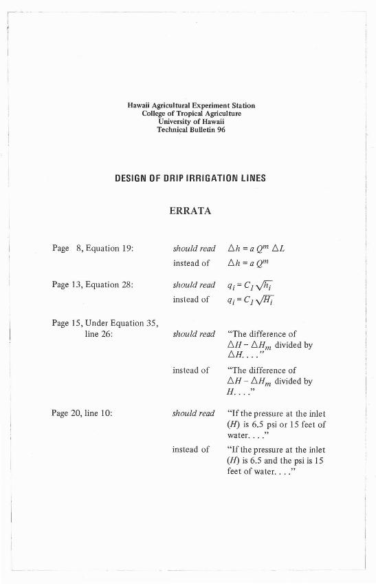
Page 8, Equation 19:
Page 13, Equation 28:
Page 15, Under Equation 35,line 26:
should read 6h =a Qm 6L
instead of 6h =a Qm
should read qi =C j Vhfinstead of qi =C j y'Hj
should read "The difference of6H - 6Hm divided by6H... . "
instead of "The difference of6H - 6Hm divided byH .. . ."
Page 20, line 10: should read "If the pressure at the inlet(H) is 6.5 psi or 15 feet ofwater. ..."
instead of "If the pressure at the inlet(H) is 6.5 and the psi is 15feet of water. ..."
CONTENTS
PAGE
In trodu ction " 3Friction Drop 4
Low F low in a Small Tubing . . . . . . . . . . . . . . . . . . . . . . . . . . .. 4Along a Lat eral Lin e . . . . 6
Pressure Distribution 10Pressure Affected by Slo pes 10Alon g a Dri p Lin e . . . . . . . . . . . . . . . . . . . . . . . . . . . . . . . . . . . . 11
Emitter Discharge 13Along a Lat eral Line 13Uni form ity Coefficient 14
Design Cha rts. . . . . . . . . . . . . . . . . . . . . . . . . . . . . . . . . . . . . . . . .. 15For Laterals 15Enginee ring Application 20For Submains 2 1
Summary and Discussion 25Referen ces Cite d 27A ppendix: Notation s 28
Figures
NUMBER PAGE
1. Water distribution and pressure along a dripirrigation line. . . . . . . . . . . . . . . . . . . . . . . . . . . . . . . . . . .. 3
2. Pressure drop by friction in a Y2-inch plastic lateral line .. 53. Dimensionless curves showing the friction drop pattern
caused by laminar flow, turbulent flow in a smooth pipe,and complete turbulent flow in a lateral line . . . . . . . . . . .. 9
4. Laboratory experiments of pressure distribution alonga lateral line com pared with theoretical dimensionlesscurves 10
Sa. Pressure distribution along a drip irrigation line(down slope) 12
5b. Pressure distribution along a drip irrigation line(up slope) 12
6. Design chart of a Y2-inch lateral line (down slope) 167. Design chart of a Y2-inch lateral line (upslope) . . . . . . . .. 18
8. Relationship between discharge ratio q /q . andmax min
the uniformity coefficient 209. Design chart of a 3t4-inch submain (down slope) 21
10. Design chart of a l-inch submain (down slope) 2211. Design chart of a 1~-in ch submain (down slope) 2212. Design chart of a 1Y2-inch submain (down slope) 2313. Design chart of a %-inch su bmain (u p slope) . . . . . .. 2314. Design chart of a l-inch submain (up slope) 2415. Design chart of a 1~-i n ch submain (up slope) . . . . . . . . .. 2416 Design chart of a 1Y2-inch submain (up slope) 25
Design of Drip Irrigation Lines
I-PAI WU and H. M. GITLIN
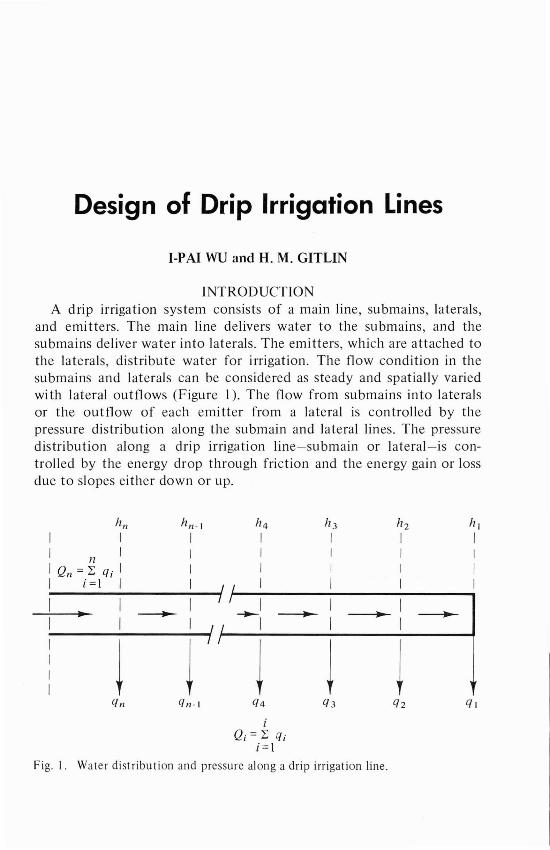
INTRODUCTIONA drip irrigation system cons ists of a main lin e, subma ins , later als,
and emitters . The main lin e deliver s wat er to th e submains , and th esubma ins deliver wa te r into lat er als. The em itters , which are attache d tothe later als, dist ribute wa ter fo r irri gation. The flow co ndit io n in th esubma ins and lat er als ca n be cons ide red as steady and spat ially va riedwith lat er al outflows (F igure I ). The flow from subma ins into later alsor the outflow of eac h emi tt er from a lat eral is con trolled by th epressure distribu tion alo ng the subma in and lat eral lin es. The press u redistribu tion along a drip irrigation lin e- submain or lat er al -is co ntrolled by the energy drop through fr ic t ion and the ene rgy gain or lossdu e to slopes eithe r down or up.
hn n«, h4 h 3 h 2 h II I I I I I II I I I I I I11
I o; =~ qi I I I I I II i =1 I I I I I I I
I I I}
I I II
.,~
~I~
I • ~I I I II
~ ~}
~ ~ ~III
qn qn-I q4 q3 q2 ql
iQi = l; a.
[ =1
Fig. 1. Water dist ribu tion and pressure along a drip irrigation line.
4 HAWAII AGRICULTURAL EXPERIMENT STATION
If the pressure distribution along a lateral line can be determined,uniform irrigation can be achieved by adjusting the size of emitters, assuggested by Myers and Bucks (4), adjusting the length and size of themicrotube-a special type of emitter used by Kenworthy (3) , or slightlyadjusting the spacing between emitters (7). If the design allows a certainvariation of emitter outflow along the lateral line , a single type ofemitter can be used, eliminating the troubles of adjustments. Thedegree of variation of emitter outflow can be shown by using theuniformity coefficient equation by Christiansen (2) (see p. 14).
The variation of discharge from emitters along a lateral line is afunction of the total length and inlet pressure, emitter spacing, andtotal flow rate. This creates a design problem to select the rightcom bination of length and pressure in order to achieve an acceptable,non-uniform pattern of irrigation.
This report presents a simple way of estimating friction drop alongthe lateral line, pressure distribution along the drip line , and variationof emitter discharge along the lateral. Design charts are presented fordetermining pressure and length of the lateral lines and submains of adrip irrigation system.
FRICTION DROP
Low Flow in a Small Tubing
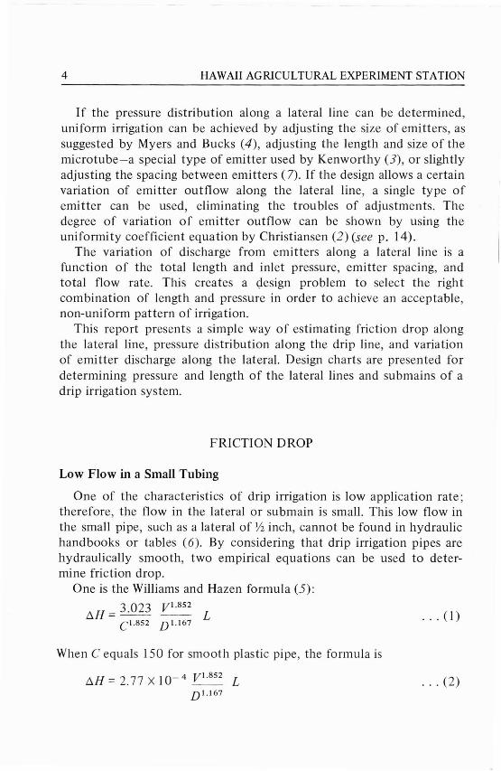
One of the characteristics of drip irrigation is low application rate;therefore, the flow in the lateral or submain is small. This low flow inthe small pipe , such as a lateral of Y2inch, cannot be found in hydraulichandbooks or tables (6). By considering that drip irrigation pipes arehydraulically smooth, two empirical equations can be used to determine friction drop.
One is the Williams and Hazen formula (5):
3.023 Vl. 852
!::..H = - - -- L ... (l)Cl. 852 D 1.167
When C equals 150 for smooth plastic pipe, the formula is
!::..H = 2.77 X 10- 4 Vl.852 LD 1.167
... (2)
DESIGN OF DRIP IRRIGATION LINES 5
... (3)
where llH is the total friction drop, in feet ; V is the m ean velocity , infeet per second; D is the diameter, in feet; and L is the pipe length, infeet.
The other is Blasius' formula (5):
[=0.3164(N )0.25
R
where [is the friction coefficient and NR
is the Reynolds number. Thefriction drop equation of pipe flow is
llH =[ ~ V2D 2g
... (4)
By combining equations 3 and 4, and simplifying, the formula becomes
VI.75llH=2.79 X 10⁻⁴ L ... (5)
D 1.25
__ Williams and Hazen_ _ _ _ Blasius
pipe diameter = J(, inch
//
I/
II
I/
//
//
/I
/I
//
//
//
/I
//
I/
//
/.....::::
b
2DISCHARGE (gpm)
Fig. 2. Pressure drop by friction in a ~-inch plastic lateral line.
6 HAWAII AGRICULTURAL EXPERIM ENT STATION
. .. (6)
It is interesting to note that equations 2 and 5 are similar- bu t with aslight differ ence. Sin ce the lat eral line is usually yz inch , a plot o ffri ction drop agains t discharge for a yz-inc h pipe, using both equations 2and 5, is shown in Figure 2. Figure 2, wh ich shows th e two curves areclose to each other, can be used to determine friction drop in th eY2-inc h lat er al line. For ot~ler sizes, use equations 2 and 5 to calculateDoH or use th e tabl es, whi ch were calcula te d by using equa tion 2, forPVC pipe.
Along a Lateral Line
The flow condition in th e lat eral line is st eady and spa tially vari edwith decreasing discharge (Figure I ) . Assume th e outflows for nsec t ions ar e ql , q 2 , q3 , ... , qn - counting from the end-and th ecorresponding pressures are hI , h2 , h 3, .. . , h n . Sin ce the end isplugged , the flow in sec tion I , whi ch is between th e outlet s I and 2, isq 1 and the flow in sec tion 2 is q 1 + q 2. The flow in eac h sec tion can beex pr essed as
i
Qj = 2: «,I
i = I , 2, 3 , ... , n
The total disch arg e supplied from th e head end is
or
nQ = 2: q,n
I. .. (7)
... (8)
The fri ction drop of pipe flow given by equa ti on 4 shows that th efri ction drop from eac h sec tion is
Doh =f Do L V2D 2g
. .. (9)
DESIGN OF DRIP IRRIGATION LINES 7
where 6.h is the friction drop at a given section and 6.L is the length ofthe section. Assume the drip line is smooth and Blasius' empiricalformula is used. By substituting equation 3 into equation 9 andsimplifying, the formula becomes
6.1z = KQI.75 6.L ... (10)
where
K = 2.53 (v)O.25 (A)O .25 _2 525 - Constant
g1T D .
where v is the kinematic viscosity. If uniform discharge is distributedfrom each outlet , the energy drop along the line can be calculated as
6.1z = K [nq] 1.75 6.Ln
6.lzn
_1
=K[(n -l)q]1.75 6.L
6./z2
= K [2q] 1.75 6.L
6./z1 = K [q] 1.75 6.L
The total energy drop will be
6.H = Kq 1.75 [n 1.75 + (n - 1) l.75 + ... 21.75 + 11.75] Ln
· .. (11)
· .. (12)
The total energy drop at the first quarter of the total length will be
6.HO
.25 = Kq l.75 [n1.75 + (n - 1)1.75 ... + (0.75n)1.75] ... (13)
The total energy drop at half the total length will be
6.H 0.5 = Kq 1.7 5 [ n 1.7 5 + (n - 1) 1.75 . . . + (0. 5n ) 1.75 ] · .. (14)
A general equation expressing the total friction at any section will be
6.H. = Kq l.75 {n1.75 + [n - 1] 1.75 ... [(1 - On ] 1.75} ... (15)I
i = 0.1, 0.2, 0.3, ... , 1.0
8 HAWAII AGRICULTURAL EXPERIMENT STATION
. .. (16)
where i represents the percentage of the length.
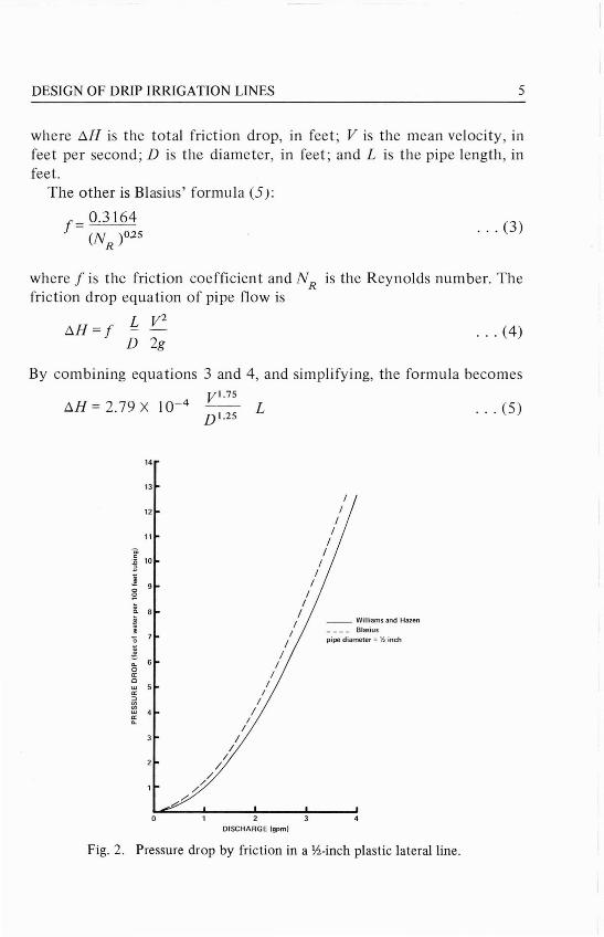
By comparing equation 15 with equation 12 the shape of the energygradient line can be determined. A computer program was made todetermine the friction drop ratio, fj,Hi/fj,H (i = 0.1, 0.2, ... ,0.9); itwas found that for different n values (50, 100, 200, ... , 1000) theratios are about the same. Therefore, the shape of the friction droppattern can be obtained. 'A dimensionless curve showing the frictiondrop ratio fj,H./fj,H and length ratio Q/L can be plotted as shown in
I
Figure 3.If the flow in each section of the drip line is small enough and the
laminar flow condition exists, then the friction coefficient is
f= 64NR
By substituting equation 16 into equation 9 and simplifying, theformula becomes
... (17)
where
K1
= 512Av = ConstantgrrD6
And , if the flow in each section is large enough so that full turbulencedevelops where the friction coefficient is a constant, the friction dropcan be expressed from equation 9 as
fj,h = K 0 2 fj,L ... (18)2 -
where
K = f = Constant2 DA 22g
Equations 17 and 18 can be used to determine the friction drop for alaminar flow and a fully turbulent flow , respectively. The differencebetween these two equations and equation lOis only the power ofdischarge. A general equation expressing friction drop can be shown as
fj,h = a Qm . .. (19)
DESIGN OF DRIP IRRIGATION LINES 9
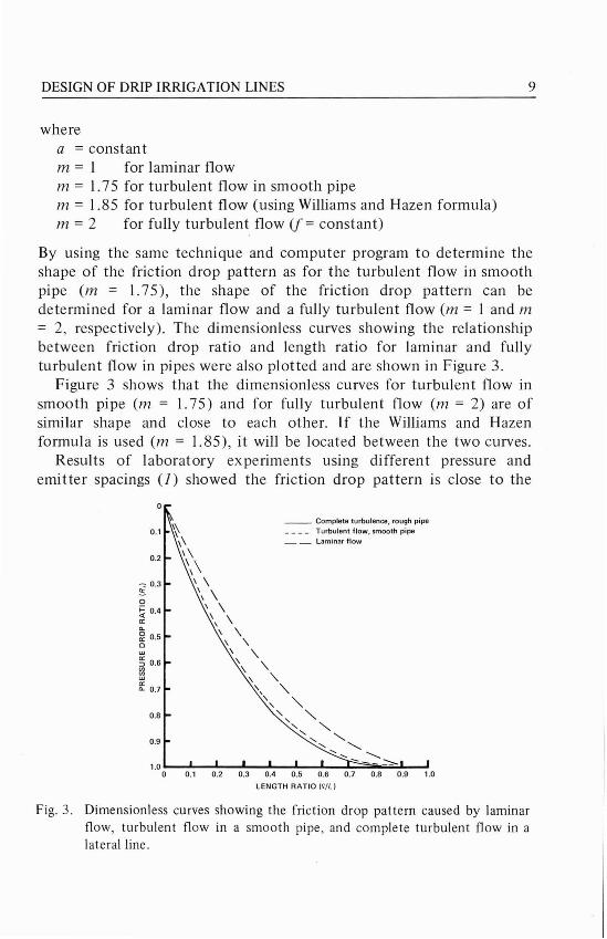
wherea = constantm = 1 for laminar flowm = 1.75 for turbulent flow in smooth pipem = 1.85 for turbulent flow (using Williams and Hazen formula)m = 2 for fully turbulent flow (j = constant)
By using the same technique and computer program to determine theshape of the friction drop pattern as for the turbulent flow in smoothpipe (m = I. 75), the shape of the friction drop pattern can bedetermined for a laminar flow and a fully turbulent flow (m = I and m= 2, respectively). The dimensionless curves showing the relationshipbetween friction drop ratio and length ratio for laminar and fullyturbulent flow in pipes were also plotted and are shown in Figure 3.
Figure 3 shows that the dimensionless curves for turbulent flow insmooth pipe (m = 1.75) and for fully turbulent flow (m = 2) are ofsimilar shape and close to each other. If the Williams and Hazenformula is used (m = 1.85) , it will be located between the two curves.
Results of laboratory experiments using different pressure andemitter spacings (1) showed the friction drop pattern is close to the
0.1
0.2
-c:: 0.3so~ 0.4a:0..
~ 0.5ow
~ 0.6~wa:0.. 0.7
0.8
0.9
__ Complete turbulence, rough pipe_ _ _ _ Turbulent flow. smooth pipe__ Laminar flow
1.0 __......._ .......--I_........_&.-........_..a....;;;;;;;;;;ii;",,;;;,,;;;;;.&..---I
a 0.1 0.2 0.3 0.4 0.5 0.6 0.7 0.8 0.9 1.0
LENGTH RATIO ( ~/L)
Fig. 3. Dimensionless curves showing the friction drop pattern caused by laminarflow, turbulent flow in a smooth pipe , and complete turbulent flow in alateral line.
10 HAWAII AGRICULTURAL EXPERIMENT STATION
__ Complete turbulence, rough pipe_ _ _ _ Turbulent flow, smooth pipe__ Lamin ar flow
0.8 0.90.3 0.4 0.5 0.6 0.7LENGTH RATIO ( ~/L)
1.0
1/ = 4 '35'35'~4 '
Exp crime nral d .uaL = ~OO M . = (,(J "
~OO ~() "
~OO 15"20() ~O "
o(-)
~
0.20.1
0.8
0.9
-:: 0.3so~ 0.4CCc..~ 0.5cw
gj 0.6en~CCc.. 0.7
Fig. 4. Laboratory experiments of pressure distribution along a lateral linecompared with theoretical dimensionless curves.
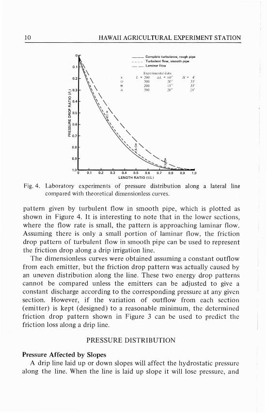
pattern given by turbulent flow in smooth pipe , which is plotted asshown in Figure 4. It is interesting to note that in the lower sections,where the flow rate is small , the pattern is approaching laminar flow.Assuming there is only a small portion of laminar flow, the frictiondrop pattern of turbulent flow in smooth pipe can be used to representthe friction drop along a drip irrigation line.
The dimensionless curves were obtained assuming a constant outflowfrom each emitter, but the friction drop pattern was actually caused byan uneven distribution along the line. These two energy drop patternscannot be compared unless the emitters can be adjusted to give aconstant discharge according to the corresponding pressure at any givensection. However, if the variation of outflow from each section(emitter) is kept (designed) to a reasonable minimum, the determinedfriction drop pattern shown in Figure 3 can be used to predict thefriction loss along a drip line.
PRESSURE DISTRIBUTION
Pressure Affected by SlopesA drip line laid up or down slopes will affect the hydrostatic pressure
along the line. When the line is laid up slope it will lose pressure, and
DESIGN OF DRIP IRRIGATION LINES 11
· .. (20)
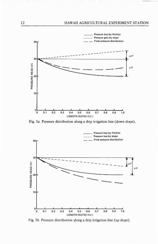
when the line is laid down slope it will gain pressure. The loss or gain inpressure is linearly proportional to the slope and length of the line.
Along a Drip LineThe total energy at any section of a drip line can be expressed by the
formula
H=Z+h + V22g
where H is the total energy expressed in feet, Z is the potential head, orelevation, in feet, h is the pressure head, in feet, and V2 /2g is thevelocity head, in feet. The change of energy with respect to the lengthof line can be expressed as
V2d(-)
dH = dZ + dh + 2g
dL dL dL dL· . . (21)
· .. (22)
Considering the outflow from emitters is low, the change of velocityhead wi th respect to the length (dL) is small and neglected. Therefore,the energy equation can be reduced to
dH = dZ + dlzdL dL dL
where dH/dL is the slope of energy line or energy slope, then
dH
dL· .. (23)
The minus sign means friction loss with respect to the length. ThedZ/dL represents the slope of the line , as in
dZ- = - S o (down slope) ... (24)dL
and
dZ
dLSo (up slope) · .. (25)
12 HAWAII AGRICULTURAL EXPERIMENT STATION
40
__ Pressure loss by friction_ _ _ _ Pressure gain by slope
__ Final pressure distribution
- ------------
----s«
30!"c;~=-=-------------------------I1_
~o<iwJ:w 20a:::>enenwa:a.
t:.H
10
1.00.20.1O.....-""""-----I--..I-----&.--........--'----II---~-.....I.---'o 0.3 0.4 0.5 0.6 0.7 0.8 0.9
LENGTH RATIO (Q!L)
Fig. Sa. Pressure distribution along a drip irrigation line (down slope).
40
__ Pressure loss by friction_ _ _ _ Pressure loss by slope__ Final pressure distribution
30"---=,....-----------------------......-__
-- -
-- --
2;o<iwJ:w 20a:::>~wa:a.
---
---- ------ - --- s n:
t:.H
10
OL.-_~_ ___I__.L__ __&.__.L__...&.._ __II___~_ ___I_ __'
o 0.1 0.2 0.3 0.4 0.5 0.6 0.7 0 .8 0.9 1.0
LENGTH RATIO (Q!L)
Fig. Sb. Pressure distribution along a drip irrigation line (up slope).
----- ---- -~ . - ._------
DESIGN OF DRIP IRRIGATION LINES
The pressure dist ribution for a drip line if it is laid down slope is
13
The pressure distribution for a drip line if it is laid up slope is
dhdL = - So -Sf
... (26)
... (27)
If the dimensionless curve (turbulent flow in smooth pipe) shown inFigure 3 can be used, the friction drop at any given length of the linecan be predicted when a total energy loss (6J.H) is known. If the length ofline and slope are known, the pressure head gain or drop (6J.H') at anysection of the line can be calculated. The pressure distribution along adrip line, if an initial pressure is given , can be determined fromequations 26 and 27, as shown in Figures Sa and 5b.
EMITTER DISCHARGE
Along a Lateral LineThe discharge (emitter outflow) at any section of a drip line is
controlled by the pressure at that section. Hydraulically the emitterou tflow is a function of the square root of the pressure, as in
a. = C !Jr (28)I 1 Vfli ...
where C1
is a coefficient and a constan t, qi is the emitter discharge atth e .th section, and hi is the pr essure at th e ith section.
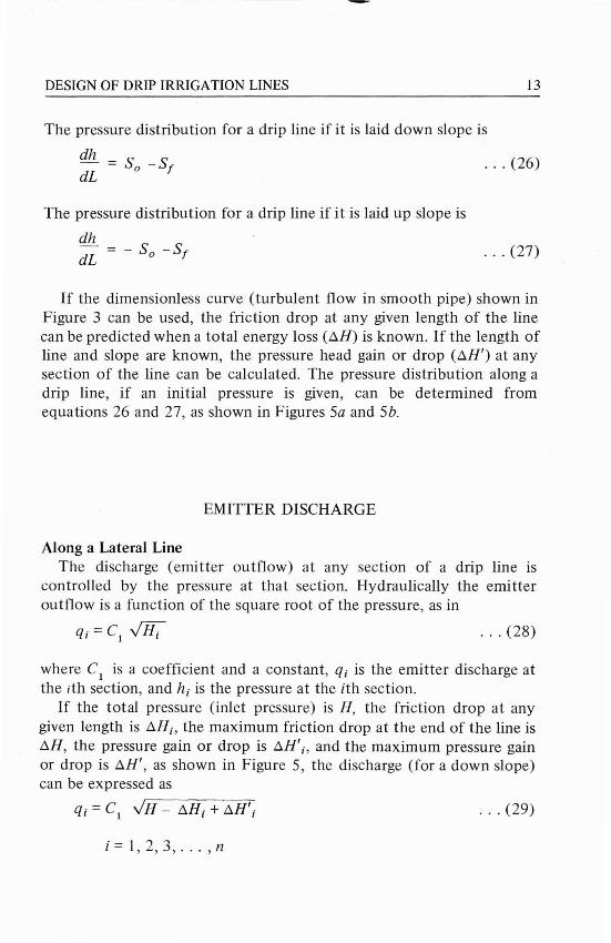
If the total pressure (inl et pressure) is H, the friction drop at anygiven length is 6J.Hi, the maximum friction drop at the end of the line is6J.H, the pre ssure gain or drop is 6J.H'i , and the maximum pressure gainor drop is 6J.H' , as shown in Figure 5, the discharge (for a down slope)can be ex pressed as
q, =C1 vlH - 6J.Hi + 6J.H'i ... (29)
i= 1, 2,3 , ... , n
14 HAWAII AGRICULTURAL EXPERIMENT STATION
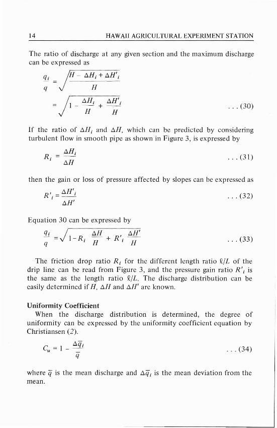
The ratio of discharge at any given section and the maximum dischargecan be expressed as
qi /H - f1H, + f1H',
q .... H
j f1H AH'·__I· .. (30)= 1 - HI +
H
If the ratio of AHi and AH, which can be predicted by consideringturbulent flow in smooth pipe as shown in Figure 3, is expressed by
AH·R. = __I
1 AH · .. (31)
· .. (32)
then the gain or loss of pressure affected by slopes can be expressed as
R'. = AR'i1
AH'
Equation 30 can be expressed by
q, J AH AH'-; = 1- n, H + ir, H · .. (33)
... (34)
The friction drop ratio R, for the different length ratio QjL of thedrip line can be read from Figure 3, and the pressure gain ratio R', isthe same as the length ratio QjL. The discharge distribution can beeasily determined if H, AH and AH' are known.
Uniformity CoefficientWhen the discharge distribution is determined, the degree of
uniformity can be expressed by the uniformity coefficient equation byChristiansen (2).
C = 1 _ Aqiu _q
where q is the mean discharge and Aqi is the mean deviation from themean.
DESIGN OF DRIP IRRIGATION LINES
DESIGN CHARTS
15
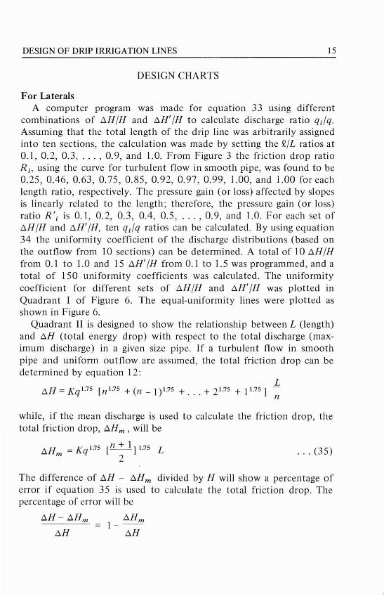
For LateralsA computer program was made for equation 33 using different
combinations of 6.H/H and 6.H' /H to calculate discharge ratio q.lq.Assuming that the total length of the drip line was arbitrarily assignedinto ten sections, the calculation was made by setting the £/L ratios at0.1,0.2,0.3, ... ,0.9, and 1.0. From Figure 3 the friction drop ratioRi, using the curve for turbulent flow in smooth pipe, was found to be0.25,0.46,0.63,0.75,0.85,0.92,0.97,0.99, 1.00, and 1.00 for eachlength ratio, respectively. The pressure gain (or loss) affected by slopesis linearly related to the length; therefore, the pressure gain (or loss)ratio R', is 0.1,0.2,0.3,0.4,0.5, ... ,0.9, and 1.0. For each set of6.H/H and 6.H' /H, ten q;/q ratios can be calculated. By using equation34 the uniformity coefficient of the discharge distributions (based onthe outflow from 10 sections) can be determined. A total of 10 6.H/Hfrom 0.1 to 1.0 and 15 6.H' /H from 0.1 to 1.5 was programmed, and atotal of 150 uniformity coefficients was calculated. The uniformitycoefficient for different sets of 6.H/H and 6.H' /H was plotted inQuadrant I of Figure 6. The equal-uniformity lines were plotted asshown in Figure 6.
Quadrant II is designed to show the relationship between L (length)and 6.H (total energy drop) with respect to the total discharge (maximum discharge) in a given size pipe. If a turbulent flow in smoothpipe and uniform outflow are assumed, the total friction drop can bedetermined by equation 12:
L6.H = Kq 1.75 [n 1.75 + (n _ 1) 1.75 + ... + 21.75 + 11.75] --;;
while, if the mean discharge is used to calculate the friction drop, thetotal friction drop, 6.Hm , will be
n + 16.H = Kq1.75 [- -] 1.75 L (35)m 2 ...
The difference of 6.H - 6.Hm divided by H will show a percentage oferror if equation 35 is used to calculate the total friction drop. Thepercentage of error will be
6.H - 6.Hm 6.Hm1--6.H 6.H
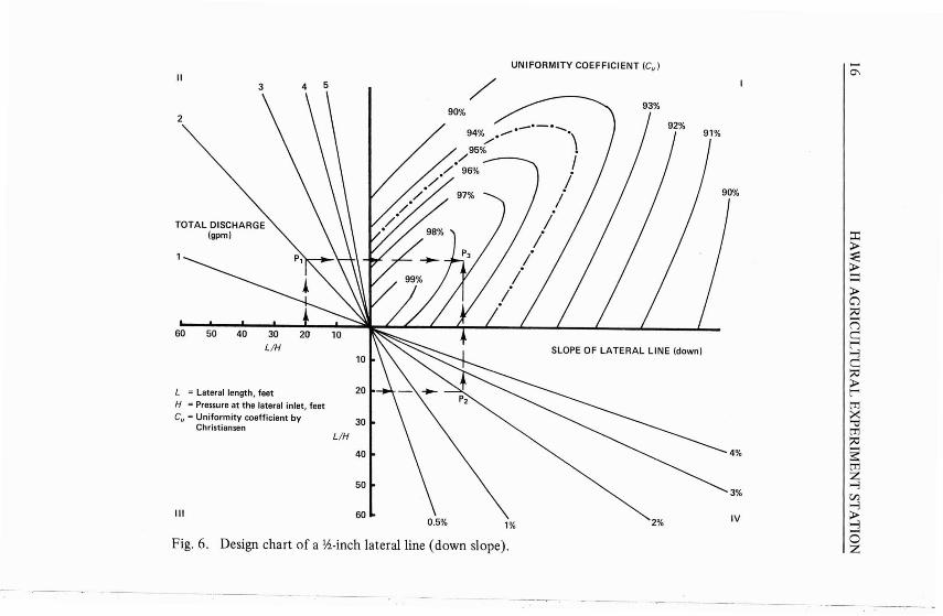
Fig . 6. Design chart of a ~-inch lateral line (down slope) .
L = Lateral length, feetH = Pressure at the lateral inlet, feetCu = Uniformity coefficient by
Christiansen
II3
2
60 50 40 30
LlH
III
4 5
30
LlH
40
50
60
/UNIFORMITY COEFFICIENT ICu )
1%
......0\
::r::>::EE;>CJC!nc:~c:~t'"""tTl
?dtTl~
4% I~tTlZ
3% ,--3en--3
IV I>--3<3z
DESIGN OF DRIP IRRIGATION LINES
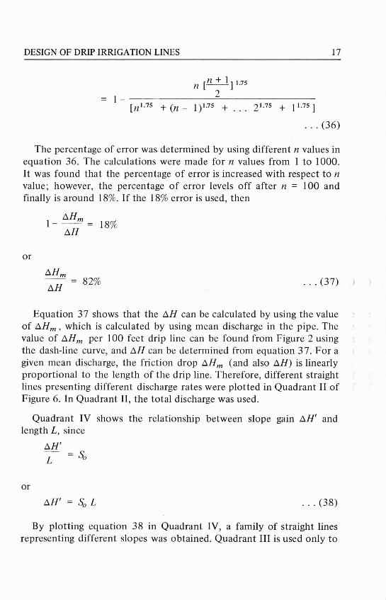
n [n + 1] 1.75
1_ 2[n1.75 + (n - 1)1.75 + . .. 21.75 + 11.75]
17
.. . (36)
The percentage of error was determined by using different n values inequation 36. The calculations were made for n values from 1 to 1000.H was found that the percentage of error is increased with respect to nvalue ; however, the percentage of error levels off after n = 100 andfinally is around 18%. If the 18% error is used, then
!J.Hm1 - - -= 18%
!J.H
or
!J.Hm
!J.H82% ... (37)
Equation 37 shows that the !J.H can be calculated by using the valueof !J.Hm , which is calculated by using mean discharge in the pipe. Thevalue of !J.Hm per 100 feet drip line can be found from Figure 2 usingthe dash-line curve, and !J.H can be determined from equation 37 . For agiven mean discharge, the friction drop !J.Hm (and also !J.H) is linearlyproportional to the length of the drip line. Therefore, different straightlines presenting different discharge rates were plotted in Quadrant II ofFigure 6. In Quadrant II, the total discharge was used.
Quadrant IV shows the relationship between slope gain !J.H' andlength L, since
!J.H'
L
or
... (38)
By plotting equation 38 in Quadrant IV, a family of straight linesrepresenting different slopes was obtained. Quadrant III is used only to
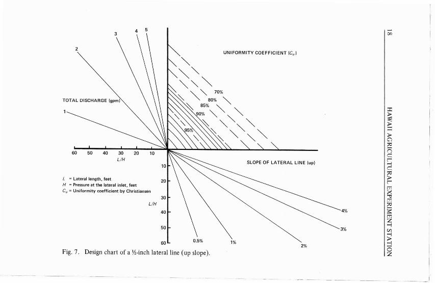
Fig . 7. Design chart of a ~-inch lateral line (up slope).
40
30
00
::r:;1>:E=::-;1>()
c:nCr'....,C10;1>r-tT:l
?atT:l10
4% ,~rnZ....,
3% len....,;1>
2% ,:j0Z
1%
UNIFORMITY COEFFICIENT (Cu )
0.5%
50
60
4 5
40 30L!H
5060
L!H
2
TOTAL DISCHARGE (gpm)
L = Lateral length, feet
H = Pressure at the lateral inlet, feet
Cu = Uniformity coefficient by Christiansen
--- - - - .- - - - ---
DESIGN OF DRIP IRRIGATION LINES 19
... (39)
show the scales of L /H, and it can be considered a design parameter.Figure 6 is a design chart; a designer can try different Ls and Hs andcheck the uniformity coefficient of the design.
The same design chart can be constructed for the drip line having anup slope merely by changing equation 33 to
fJJ = } _ R. ~H _ R' . '~H'q I H I H
and following the same procedure for designing Figure 6. The designchart for having a drip line laid up slope can be obtained and is shownin Figure 7.
Figures 6 and 7 show different uniformity patterns; Figure 6 shows ahigher uniformity pattern than Figure 5. It is reasonable to expect thehigh uniformity pattern for Figure 6 when the energy drop is combinedwith energy gain from the down slope, whereas, in Figure 7, energydrop is combined with energy loss from the up slope.
A design criterion should be set regarding the uniformity coefficientthat will be used. The concept here of uniformity coefficient should beconsidered differently from the uniformity coefficient used in sprinklerirrigation design, even though the definition and equation of uniformitycoefficient is the same. A uniformity coefficient of 80 to 90%, which isconsidered good enough, may not be acceptable in a drip irrigationdesign. A sprinkler irrigation system irrigates a whole area where watercan be redistributed easily after irrigation, whereas a drip irrigationsystem irrigates discrete points where a point of low application maywell affect the growth of crops.
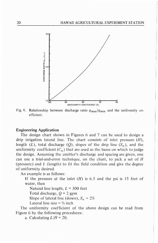
A study was made of the relation between uneven distribu tion andthe uniformity coefficient. It was found that a discharge ratioqmax /qmin can be correlated with the uniformity coefficient; this wasplotted as shown in Figure 8. Figure 8 shows that the q max is 40 %more than the qmin when the uniformity coefficient is 90%; and the qmax
is 85% more than the qmin when the uniformity coefficient is 80%.Considering the discharge variations, design criteria were set so that auniformity of 98% or more is considered to be desirable where theqmax and qmin variation is less than 10%; a uniformity coefficientfrom 95 to 98 is considered to be acceptable where the qmax and qmin
variation is less than 20%; a uniformity coefficient of less than 95% isnot recommended.
20
3.0
E~
:1oi=ct 2.0CCUJClccctJ:Ueno
HAWAII AGRlCULTURAL EXPERIMENT STATION
90 80 70 60UNIFORMITY COEFFICIENT (%)
Fig. 8. Relationship between discharge ratio qrnax/qrnin and the uniformity coefficient.
Engineering ApplicationThe design chart shown in Figures 6 and 7 can be used to design a
drip irrigation lateral line. The chart consists of inlet pressure (H),length (L), total discharge (Q), slopes of the drip line (So), and theuniformity coefficient (Cu ) that are used as the bases on which to judgethe design. Assuming the emi tter's discharge and spacing are given, onecan use a trial-and-error technique, on the chart, to pick a set of H(pressure) and L (length) to fit the field condition and give the degreeof uniformity desired.
An example is as follows:If the pressure at the inlet (H) is 6.5 and the psi is 15 feet ofwater, then
Natural line length, L = 300 feetTotal discharge, Q = 2 gpmSlope of lateral line (down) , So = 2%Lateral line size = ~ inch
The uniformity coefficient of the above design can be read fromFigure 6 by the following procedures:
a. Calculating L/H = 20.
DESIGN OF DRIP IRRIGATION LINES 21
b. Drawing a vertical dash line in Quadrant II of Figure 6 fromL [H = 20 up to meet 2 gpm discharge line at a point Pl.
c. Drawing a horizontal dash line from L [H = 20 in Quadrant IVto the right to meet the 2% slope line at a point P2.
d. Drawing a horizontal dash line from PI and a vertical line fromP2 ' so that the two lines will meet at a point , P3 ' which willshow the uniformity coefficient, Cu = 97%.
This procedure shows the design is acceptable.Suppose the same drip irrigation system is used except the line is laid
up slop e. Using the same procedure and Figure 7, the uniformitycoefficient is found to be 85%, whi ch is not acceptable.
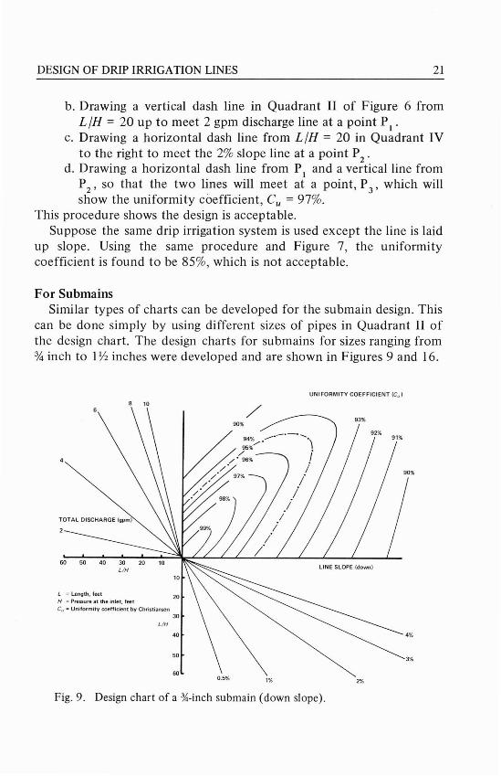
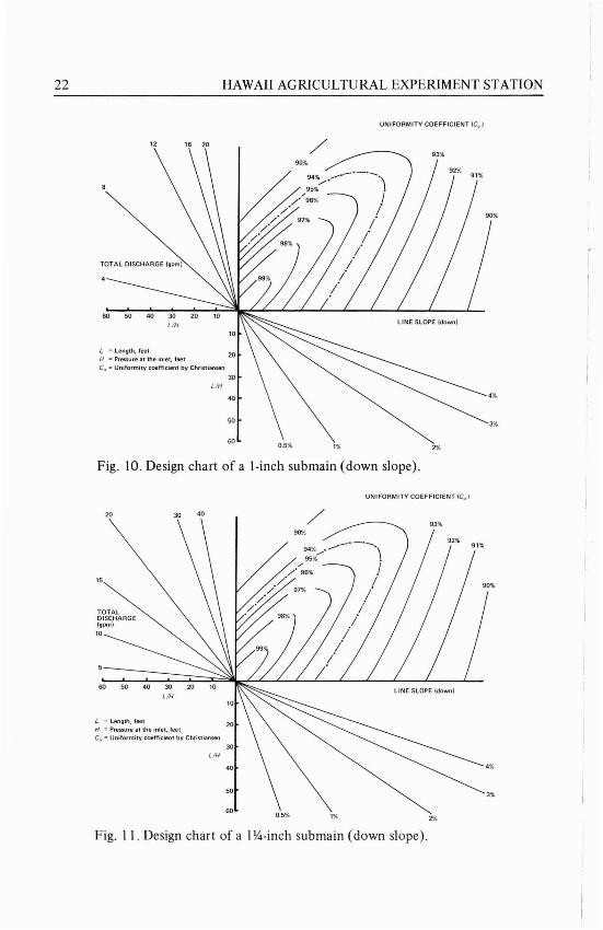
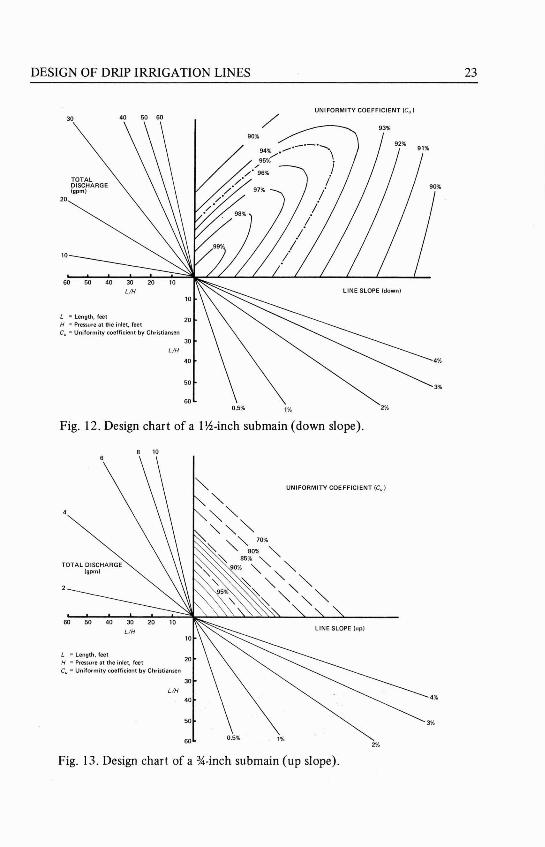
For SubmainsSimilar types of charts can be developed for th e submain design. This
can be done simply by using different sizes of pipes in Quadrant II ofthe design chart. The design charts for submains for sizes ranging from% inch to 112 inches were developed and are shown in Figures 9 and 16.
UNIFORMITY COE FFICIENT leu)
8 10
60 50 40 30 20LlH
L = Length, fee tH = Pressure at th e inlet. feetCu = Unifor mity coe fficie nt by Chr ist iansen
30LlH
40
50
600.5 % 1% 2%
Fig . 9 . Design chart of a ~-inch submain (down slope).
22 HAWAII AGRICULTURAL EXPERIMENT STATION
UN IFORM IT Y COEFFICIENT ICu )
12 16 20
60 50 40 30
LlH
L = Length, feetH = Pressure at the inlet , feetCu = Uniform ity coeff icient by Christiansen
LlH
50
600.5% 1% 2%
3%
Fig . 10. Design chart of a l-inch submain (down slope) .
UN IFO RMITY COEFF ICIENT ICu )
LlH
3%
2%1%0.5%60
50
30
40
30 4020
60 50 40 30 20
LlH
15
L = Length , feetH = Pressure at the inlet, feetCu .. Unifor mity co effi cient by Christiansen
Fig. 11. Design cha rt of a 1~-inch subma in (down slope) .
DESIGN OF DRIP IRRIGATION LINES 23
40
50
30
60
40 50 6030
60 50 40 30
LlH
LlH
10
20
L = Length. feetH = Pressureat the inlet, feeteu = Uniformity coefficient by Chri stiansen
0.5% 1% 2%
Fig. 12. Design chart of a 1~-inch submain(down slope).
10
60 50 40 30
LlH
L = Length. feetH = Pressureat the inlet, feetell::;: Uniformity coeffi cient by Christiansen
30
LlH40
50
UNIFORMITY COEFFICIENT (Cu )
4%
3%
60 0.5% 1%2%
Fig. 13. Design chart of a %-inch submain(up slope).
24
12 16 20
HAWAII AGRICULTURAL EXPERIMENT STATION
UNIFORMITY COEFF ICIEN T ICu )
60 50 40 30L/H
L = Len gth, feelH = Pressure at the inlet, feetCu = Uniformity coeffic ient by Christiansen
30
L/H
40
50
60 1%2%
4%
3%
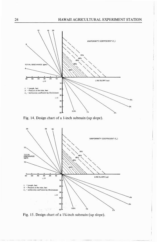
Fig. 14. Design chart of a l-inch submain (up slope).
20 30 40
15
10
60 50 40 30 20
L/H
L = Len gth , feelH = Pressure at the inlet, feetCu = Uniformity coeffi cient by Christiansen
30
L/H
40
50
600.5 % 1%
UNIFORMITY COEFFICIENT (Cu I
2%
4%
Fig. 15. Design chart of a 1~-inch submain (up slope).
DESIGN OF DRIP IRRIGATION LINES
30 40 50 60
20
10
60 50 40 30L/H
L = Length, feetH = Pressure at the inlet . feetCu =Uniformity coeff icient by Christiansen
30
L/H
40
50
UNIFORMITY COEFFICIENT (Cu )
4%
3%
25
600.5% 1% 2%
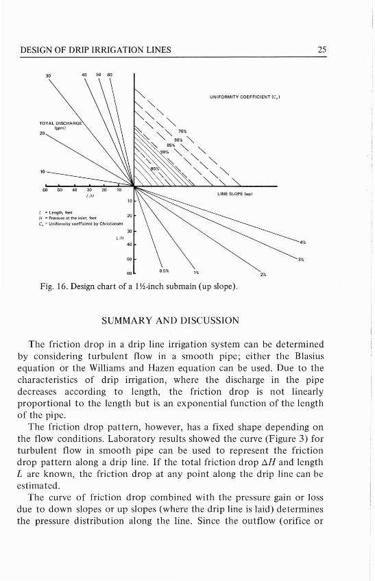
Fig . 16. Design chart ofa l~-inch submain (up slope).
SUMMARY AND DISCUSSION
The friction drop in a drip line irrigation system can be determinedby considering turbulent flow in a smooth pipe; either the Blasiusequation or the Williams and Hazen equation can be used. Due to thecharacteristics of drip irrigation, where the discharge in the pipedecreases according to length, the friction drop is not linearlyproportional to the length but is an exponential function of the lengthof the pipe.
The friction drop pattern, however, has a fixed shape depending onthe flow conditions. Laboratory results showed the curve (Figure 3) forturbulent flow in smooth pipe can be used to represent the frictiondrop pattern along a drip line. If the total friction drop t1H and lengthL are known, the friction drop at any point along the drip line can beestimated.
The curve of friction drop combined with the pressure gain or lossdue to down slopes or up slopes (where the drip line is laid) determinesthe pressure distribution along the line. Since the outflow (orifice or
26 HAWAIIAGRICULTURAL EXPERIMENT STATION
emitter outflow) is controlled by the pressure, if the pressuredistribution is known, the emitter discharge distribution can bedetermined. A uniformity coefficient can be calculated from thedischarge distribution.
A design chart has been int roduced , consisting of design pressure andlength of the drip line , total discharge , slope of the line , and uniformitycoefficient. The chart will help to design a drip irrigation line based ona desirable or acceptable uniformity. The designer can try differentcombinations of pressure (H) and length (L) in order to obtain one thatis acceptable and fits the field condition.
The same design chart can be made for up slope conditions, whichlose pressure with respect to the length, and for the different sizes ofpipes that may be used for submain line design.
DESIGN OF DRIP IRRIGATION LINES
REFERENCES CITED
27
1. Bui , U. Hydraulics of trickle irrigation lines. Univ. Hawaii , M.S.Thesis. September 1972.
2. Christiansen, J. E. Hydraulics of sprinkling systems for irrigation.Trans. ASCE 107 :221-239. 1942.
3. Kenworthy, A. L. Trickle irrigation-the concept and guideline foruse. Michigan Agr. Exp. Sta. Res. Rep. 165 (Farm Science). May1972.
4. Myers, L. E., and D. A. Bucks. Uniform irrigation with low-pressuretrickle system. J. Irrig. Drainage Div., ASCE Proc. Paper 917598(IR3):341-346. September 1972.
5. Rouse, H., and J. W. Howe. Basic mechanics of fluids. New York:John Wiley and Sons. 1953.
6. Williams, G. S., and A. Hazen. Hydraulic tables. 3rd ed. New York:John Wiley and Sons. 1960.
7. Wu, I. P., and H. M. Gitlin. Hydraulics and uniformity for dripirrigation. J. Irrig. Drainage Div., ASCE Proc. Paper 9786 99(IR3):157-168. June 1973.
28 HAWAII AGRICULTURAL EXPERIMENT STATION
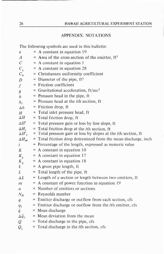
APPENDIX: NOTATIONS
The following symbols are used in this bulletin:a A constant in equation 19A Area of the cross section of the emitter, ft2C A constant in equation 1C
1A constant in equation 28
C; Christiansen uniformity coefficientD Diameter of the pipe, ft2f Friction coefficientg Gravitational acceleration, ft/sec 2
h Pressure head in the pipe , fthi Pressure head at the ith section, ftI::J.h Friction drop, ftH Total inlet pressure head , ftI::J.H Total friction drop, ftI::J.H' Total pressure gain or loss by line slope, ftI::J.Hi Total friction drop at the ith section, ftI::J.H'; Total pressure gain or loss by slopes at the ith section , ftI::J.Hm Total friction drop determined from the mean discharge , inchi Percentage of the length, expressed as numeric valueK A constant in equation 10K I = A constant in equation 17K
2A constant in equation 18
Q A given pipe length, ftL Total length of the pipe, ftI::J.L = Length of a section or length between two emitters, ftm A constant of power function in equation 19n = Number of emitters or sectionsN R Reynolds numberq Emitter discharge or outflow from each section, cfsqj Emitter discharge or outflow from the ith emitter, cfsq = Mean dischargeI::J.qi Mean deviation from the meanQ = Total discharge in the pipe, cfsQ; Total discharge in the ith section , cfs
DESIGN OF DRIP IRRIGATION LINES
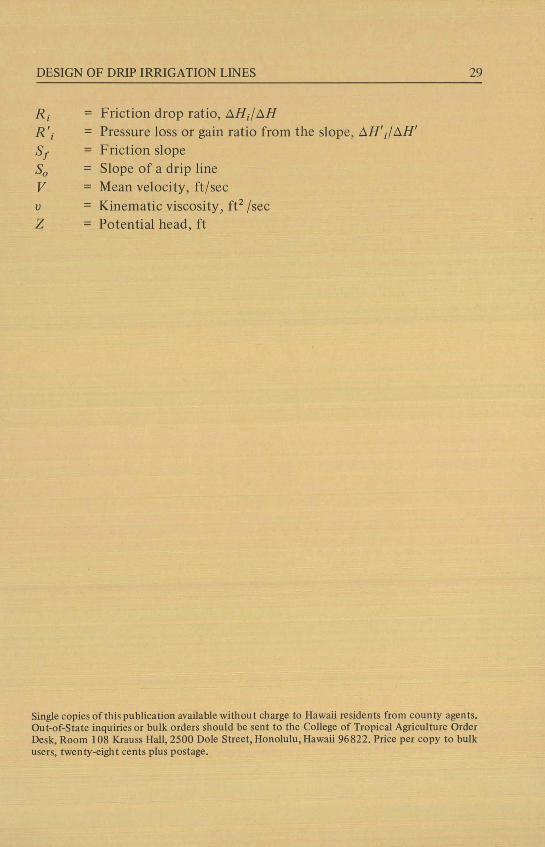
R, Friction drop ratio, 6.H)6.HR', Pressure loss or gain ratio from the slope, 6.H' J6.H'
Sf Friction slopeSo Slope of a drip lineV Mean velocity, ft/secv Kinematic viscosity i ft2 /secZ Potential head, ft
29
Single copies of this publication available withou t charge to Hawaii residen ts from coun ty agents.Out-of-State inquiries or bulk orders should be sent to the College of Tropical Agriculture OrderDesk, Room 108 Krauss Hall, 2500 Dole Street, Honolulu, Hawaii 96822. Price per copy to bulkusers, twen ty-eigh t cents plus postage.
Hawaii Agricultural Experiment StationCollege of Tropical Agriculture, University of HawaiiC. Peairs Wilson, Dean of the College and Director of the Experiment StationLeslie D. Swindale, Associate Director of the Experiment Station
Tech. Bull. 96-June 1974 (2M)


