Design of Experiments and Analysis of Variance...

Design of Experiments and Analysis of Variance Chapter 8

8.2 The treatments are the combinations of levels of each of the two factors. There are 2 × 5 = 10

treatments. They are: (A, 50), (A, 60), (A, 70), (A, 80), (A, 90) (B, 50), (B, 60), (B, 70), (B, 80), (B, 90) 8.4 a. College GPA's are measured on college students. The experimental units are college

students. b. Household income is measured on households. The experimental units are households. c. Gasoline mileage is measured on automobiles. The experimental units are the

automobiles of a particular model. d. The experimental units are the sectors on a computer diskette. e. The experimental units are the states. 8.6 a. The response variable is the amount of the purchase.

b. There is one factor in this problem: type of credit card.

c. There are 4 treatments, corresponding to the 4 levels of the factor. The treatments are VISA, MasterCard, American Express, and Discover.

d. The experimental units are the credit card holders.

8.8 a. The response variable in this problem is the consumer’s opinion on the value of the discount offer.

b. There are two treatments in this problem: Within-store price promotion and between- store price promotion.

c. The experimental units are the consumers.

8.10 a. There are 2 factors in the problem: Type of yeast and Temperature. Type of yeast has 2 levels – Brewer’s yeast and baker’s yeast. Temperature has 4 levels – 45o, 48o, 51o and 54oC.

b. The response variable is the autolysis yield.

c. There are a total of 2 × 4 = 8 treatments in this experiment. The treatments are all the type of yeast-temperature combinations.

d. This is a designed experiment.

256 Chapter 8

8.12 a. The response is the evaluation by the undergraduate student of the ethical behavior of the salesperson.

b. There are two factors—type of sales job at two levels (high tech. vs. low tech.) and sales

task at two levels (new account development vs. account maintenance). c. The treatments are the 2 × 2 = 4 combinations type of sales job and sales task. d. The experimental units are the college students. 8.14 a. From Table IX with ν1 = 4 and ν2 = 4, F.05 = 6.39. b. From Table XI with ν1 = 4 and ν2 = 4, F.01 = 15.98. c. From Table VIII with ν1 = 30 and ν2 = 40, F.10 = 1.54. d. From Table X with ν1 = 15, and ν2 = 12, F.025 = 3.18. 8.16 a. In the second dot diagram #2, the difference between the sample means is small relative

to the variability within the sample observations. In the first dot diagram #1, the values in each of the samples are grouped together with a range of 4, while in the second diagram #2, the range of values is 8.

b. For diagram #1,

11

7 8 9 10 11 546 6

xx

n+ + + +

= = =∑ = 9

22

12 13 14 14 15 16 846 6

xx

n+ + + + +

= = =∑ = 14

For diagram #2,

11

5 5 7 11 13 13 546 6

xx

n+ + + + +

= = =∑ = 9

22

10 10 12 16 18 18 846 6

xx

n+ + + + +

= = =∑ = 14

c. For diagram #1,

SST = 2

2

1(i i

in x x

=

−∑ ) 1 = 6(9 − 11.5)2 + 6(14 − 11.5)2 = 75

54 84 11.512

xx

n⎛ ⎞+

= = =⎜ ⎟⎜ ⎟⎝ ⎠

∑

For diagram #2,

SST = 2

2

1(i i

in x x

=

−∑ ) = 6(9 - 11.5)2 + 6(14 - 11.5)2 = 75

Design of Experiments and Analysis of Variance 257

d. For diagram #1,

21s =

( )2212

11

1

544966

1 6

xx

nn

− −=

− −

∑∑1

=

2544966

6 1

−

− = 2

22s =

( )2222

22

2

8411866

1 6

xx

nn

− −=

− −

∑∑1

= 2

SSE = (n1 − 1) 2

1s + (n2 − 1) 22s = (6 − 1)2 + (6 − 1)2 = 20

For diagram #2,

21s =

( )2212

11

1

545586

1 6

xx

nn

− −=

− −

∑∑1

= 14.4

22s =

( )2222

22

2

8412486

1 6

xx

nn

− −=

− −

∑∑1

= 14.4

SSE = (n1 − 1) 2

1s + (n2 − 1) 22s = (6 − 1)14.4 + (6 − 1)14.4 = 144

e. For diagram #1, SS(Total) = SST + SSE = 75 + 20 = 95

SST is SST 75 100% = 100%SS(Total) 95

× × = 78.95% of SS(Total)

For diagram #2, SS(Total) = SST + SSE = 75 + 144 = 219

SST is SST 75 100% = 100%SS(Total) 219

× × = 34.25% of SS(Total)

f. For diagram #1, MST = SST 75 1 2 1k

=− −

= 75

MSE = SSE 20 12 2n k

=− −

= 2 F = MST 75= MSE 2

= 37.5

For diagram #2, MST = SST 75 1 2 1k

=− −

= 75

MSE = SSE 144 12 2n k

=− −

= 14.4 F = MST 75 = MSE 14.4

= 5.21

258 Chapter 8

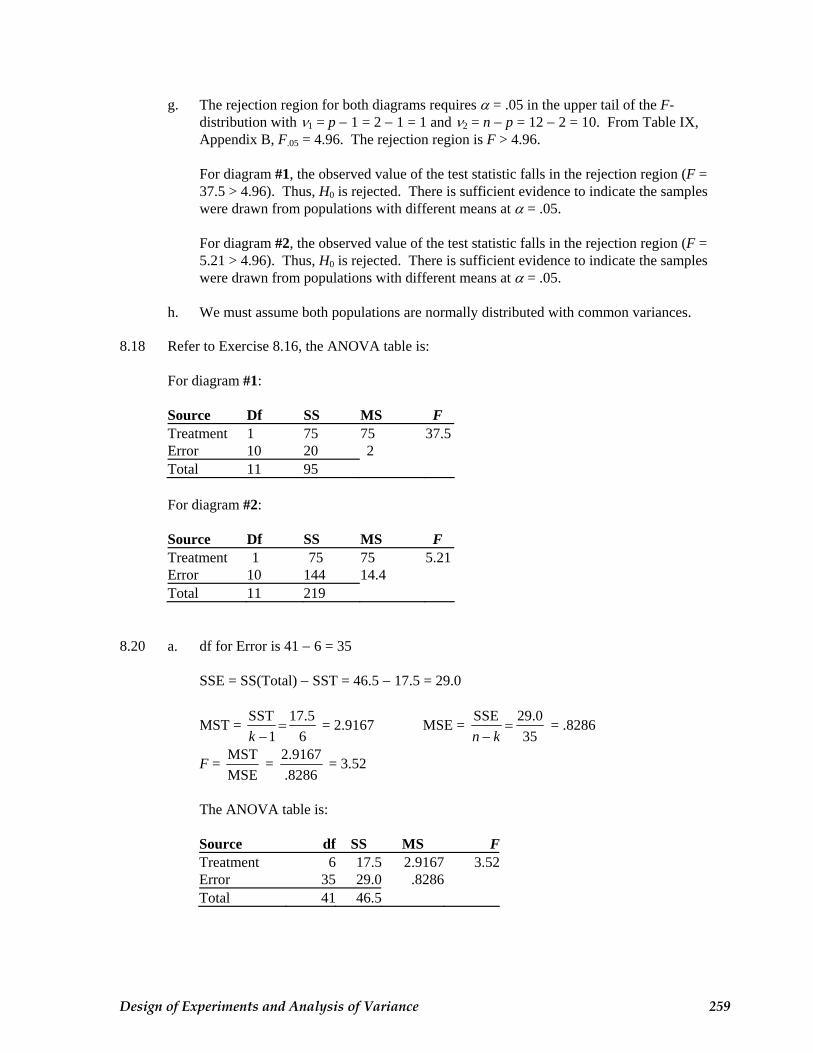
g. The rejection region for both diagrams requires α = .05 in the upper tail of the F-distribution with ν1 = p − 1 = 2 − 1 = 1 and ν2 = n − p = 12 − 2 = 10. From Table IX, Appendix B, F.05 = 4.96. The rejection region is F > 4.96.

For diagram #1, the observed value of the test statistic falls in the rejection region (F =

37.5 > 4.96). Thus, H0 is rejected. There is sufficient evidence to indicate the samples were drawn from populations with different means at α = .05.

For diagram #2, the observed value of the test statistic falls in the rejection region (F =

5.21 > 4.96). Thus, H0 is rejected. There is sufficient evidence to indicate the samples were drawn from populations with different means at α = .05.

h. We must assume both populations are normally distributed with common variances. 8.18 Refer to Exercise 8.16, the ANOVA table is: For diagram #1:

Source Df SS MS F Treatment 1 75 75 37.5Error 10 20 2 Total 11 95

For diagram #2:

Source Df SS MS F Treatment 1 75 75 5.21Error 10 144 14.4 Total 11 219

8.20 a. df for Error is 41 − 6 = 35 SSE = SS(Total) − SST = 46.5 − 17.5 = 29.0

MST = SST 17.5 1 6k

=−

= 2.9167 MSE = SSE 29.0 35n k=

− = .8286

F = MST 2.9167 = MSE .8286

= 3.52

The ANOVA table is:

Source df SS MS F Treatment 6 17.5 2.9167 3.52Error 35 29.0 .8286Total 41 46.5


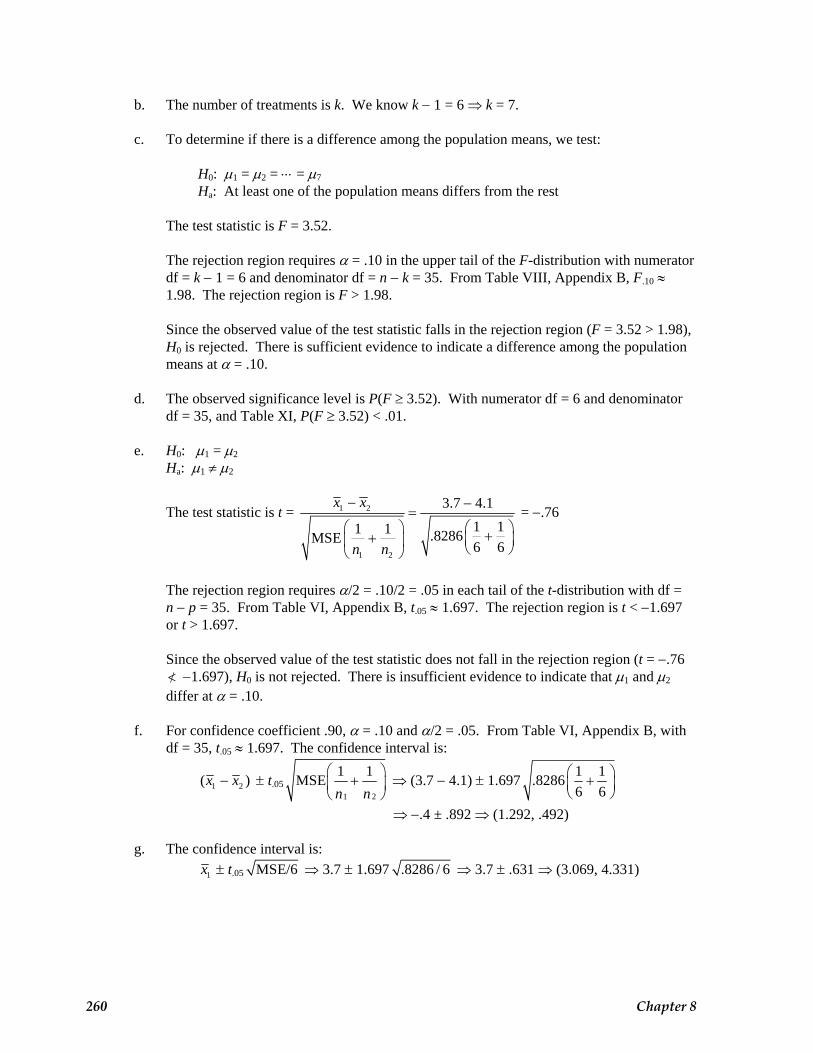
b. The number of treatments is k. We know k − 1 = 6 ⇒ k = 7. c. To determine if there is a difference among the population means, we test: H0: μ1 = μ2 = ⋅⋅⋅ = μ7

Ha: At least one of the population means differs from the rest The test statistic is F = 3.52. The rejection region requires α = .10 in the upper tail of the F-distribution with numerator

df = k − 1 = 6 and denominator df = n − k = 35. From Table VIII, Appendix B, F.10 ≈ 1.98. The rejection region is F > 1.98.

Since the observed value of the test statistic falls in the rejection region (F = 3.52 > 1.98),

H0 is rejected. There is sufficient evidence to indicate a difference among the population means at α = .10.

d. The observed significance level is P(F ≥ 3.52). With numerator df = 6 and denominator

df = 35, and Table XI, P(F ≥ 3.52) < .01. e. H0: μ1 = μ2

Ha: μ1 ≠ μ2

The test statistic is t = 1 2

1 2

3.7 4.11 11 1 .8286MSE 6 6

x x

n n

− −=

⎛ ⎞ ⎛ ++ ⎜ ⎟⎜ ⎟ ⎝ ⎠⎝ ⎠

⎞ = −.76

The rejection region requires α/2 = .10/2 = .05 in each tail of the t-distribution with df =

n − p = 35. From Table VI, Appendix B, t.05 ≈ 1.697. The rejection region is t < −1.697 or t > 1.697.

Since the observed value of the test statistic does not fall in the rejection region (t = −.76

</ −1.697), H0 is not rejected. There is insufficient evidence to indicate that μ1 and μ2 differ at α = .10.

f. For confidence coefficient .90, α = .10 and α/2 = .05. From Table VI, Appendix B, with

df = 35, t.05 ≈ 1.697. The confidence interval is:

1 2( )x x− ± t.051 2

1 1MSE n n

⎛+⎜

⎝ ⎠

⎞⎟ ⇒ (3.7 − 4.1) ± 1.697 1 1.8286

6 6 ⎛ ⎞+⎜ ⎟

⎝ ⎠

⇒ −.4 ± .892 ⇒ (1.292, .492) g. The confidence interval is: 1x ± t.05 MSE/6 ⇒ 3.7 ± 1.697 .8286 / 6 ⇒ 3.7 ± .631 ⇒ (3.069, 4.331)

260 Chapter 8

8.22 a. The experimental unit in the study is the college tennis coach. The dependent variable is the response to the statement “the Prospective Student-Athlete Form on the web site contributes very little to the recruiting process” on a scale from 1 to 7. There is one factor in the study and it is the NCAA division of the college tennis coach. There are 3 levels of this factor, and thus, there are 3 treatments – Division I, Division II, and Division III.

b. To determine if the mean responses of tennis coaches from the different divisions differ, we test:

H0: μ1 = μ2 = μ3

Ha: At least 1 μi differs

c. Since the observed p-value of the test (p < .003) is less than α = .05, H0 is rejected. There is sufficient evidence to indicate differences in mean response among coaches of the 3 divisions.

8.24 a. A completely randomized design was used.

b. There are 4 treatments: 3 robots/colony, 6 robots/colony, 9 robots/colony, and 12 robots/colony.

c. To determine if there was a difference in the mean energy expended (per robot) among

the 4 colony sizes, we test:

H0: μ1 = μ2 = μ3 = μ4 Ha: At least two means differ

d. Since the p-value (<.001) is less than α (.05), H0 is rejected. There is sufficient evidence

to indicate a difference in mean energy expended per robot among the 4 colony sizes at α = .05.

8.26 a. To determine if differences exist in the mean rates of return among the three types of fund groups, we test: H0: μ1 = μ2 = μ3

Ha: At least two means differ

b. The rejection region requires α = .01 in the upper tail of the F-distribution with ν1 = k – 1 = 3 – 1 = 2 and ν2 = N – k = 90 – 3 = 87. From Table XI, Appendix B, F.01 ≈ 4.98. The rejection region is F > 4.98.

c. Since the observed value of the test statistic falls in the rejection region (F = 69.65 >

4.98), H0 is rejected. There is sufficient evidence to indicate differences exist in the mean rates of return among the three types of fund groups at α = .01.


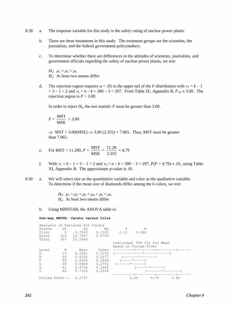
8.28 a. The response variable for this study is the safety rating of nuclear power plants. b. There are three treatments in this study. The treatment groups are the scientists, the

journalists, and the federal government policymakers. c. To determine whether there are differences in the attitudes of scientists, journalists, and

government officials regarding the safety of nuclear power plants, we test: H0: μ1 = μ2 = μ3

Ha: At least two means differ d. The rejection region requires α = .05 in the upper tail of the F-distribution with ν1 = k − 1

= 3 − 1 = 2 and ν2 = n − k = 300 − 3 = 297. From Table IX, Appendix B, F.05 ≈ 3.00. The rejection region is F > 3.00.

In order to reject H0, the test statistic F must be greater than 3.00.

F = MSTMSE

> 3.00

⇒ MST > 3.00(MSE) ⇒ 3.00 (2.355) = 7.065. Thus, MST must be greater than 7.065.

e. For MST = 11.280, F = MST 11.28 = MSE 2.355

= 4.79

f. With ν1 = k − 1 = 3 − 1 = 2 and ν2 = n − k = 300 − 3 = 297, P(F > 4.79) ≈ .01, using Table

XI, Appendix B. The approximate p-value is .01. 8.30 a. We will select size as the quantitative variable and color as the qualitative variable. To determine if the mean size of diamonds differ among the 6 colors, we test:

H0: μ1 = μ2 = μ3 = μ4 = μ5 = μ6


b. Using MINITAB, the ANOVA table is:

One-way ANOVA: Carats versus Color

Analysis of Variance for Carats Source DF SS MS F P Color 5 0.7963 0.1593 2.11 0.064 Error 302 22.7907 0.0755 Total 307 23.5869 Individual 95% CIs For Mean Based on Pooled StDev Level N Mean StDev ----------+---------+---------+------ D 16 0.6381 0.3195 (-------------*------------) E 44 0.6232 0.2677 (-------*-------) F 82 0.5929 0.2648 (-----*-----) G 65 0.5808 0.2792 (------*------) H 61 0.6734 0.2643 (------*------) I 40 0.7310 0.2918 (-------*--------) ----------+---------+---------+------ Pooled StDev = 0.2747 0.60 0.70 0.80

262 Chapter 8

The test statistic is F = 2.11 and the p-value is p = 0.064.

Since the p-value (0.064) is less than α = .10, H0 is rejected. There is sufficient evidence to indicate the mean size of diamonds differ among the 6 colors at α = .10.

c. We will check the assumptions of normality and equal variances. Using MINITAB, the

stem-and-leaf plots are: Stem-and-Leaf Display: Carats Stem-and-leaf of Carats Color= 1 N = 16 Leaf Unit = 0.010 1 1 9 3 2 01 5 3 01 5 4 7 5 23 7 6 (4) 7 1156 5 8 5 9 5 10 00011 Stem-and-leaf of Carats Color = 2 N = 44 Leaf Unit = 0.010 1 1 9 4 2 123 11 3 0011345 12 4 6 (11) 5 00012245668 21 6 23 19 7 000123 13 8 113 10 9 10 10 0000011113 Stem-and-leaf of Carats Color = 3 N = 82 Leaf Unit = 0.010 5 1 88999 12 2 1356667 23 3 01124445567 27 4 0178 (21) 5 000111122333345566678 34 6 0 33 7 00001112367 22 8 0012555 15 9 0 14 10 00000011112224 Stem-and-leaf of Carats Color = 4 N = 65 Leaf Unit = 0.010 5 1 88899 12 2 0001359 21 3 000124455 23 4 08 (12) 5 000013556789 30 6 0034 26 7 0000001348 16 8 0125 12 9 12 10 000000011126


Stem-and-leaf of Carats Color = 5 N = 61 Leaf Unit = 0.010 2 1 89 5 2 457 14 3 012344567 16 4 03 21 5 25778 27 6 001466 (13) 7 0001112233448 21 8 0014669 14 9 14 10 0000011111266 1 11 0

Stem-and-leaf of Carats Color = 6 N = 40 Leaf Unit = 0.010

4 2 5689 8 3 0113 11 4 115 13 5 26 15 6 25 20 7 03355 20 8 002 17 9 0 16 10 0000001111114579

The data for the 6 colors do not look particularly mound-shaped, so the assumption of normality is probably not valid. However, departures from this assumption often do not invalidate the ANOVA results. Using MINITAB, the box plots are:

IHGFED

1.1

1.0

0.9

0.8

0.7

0.6

0.5

0.4

0.3

0.2

Color

Car

ats

The spreads of all the colors appear to be about the same, so the assumption of constant variance is probably valid.

264 Chapter 8

8.32 a. The df for Groups = ν1 = k – 1 = 3 – 1 = 2. The df for Error = ν2 = n – k = 71 – 3 = 68. The completed ANOVA table is:

Source df SS MS F Groups 2 128.70 64.35 0.16 Error 68 27,124.52 398.89

b. To determine if the total number of activities undertaken differed among the three groups

of entrepreneurs, we test: H0: μ1 = μ2 = μ3

Ha: At least one mean differs The test statistic is F = 0.16. The rejection region requires α = .05 in the upper tail of the F-distribution with ν1 = k − 1


Since the observed value of the test statistic does not fall in the rejection region (F = 0.16

>/ 3.15), H0 is not rejected. There is insufficient evidence to indicate that the total number of activities differed among the groups of entrepreneurs at α = .05.

c. The p-value of the test is P(F > 0.16). From Table VIII, Appendix B, with ν1 = 2 and

ν2 = 68, P(F > 0.16) > .10. d. No. Since our conclusion was that there was no evidence of a difference in the total

number of activities among the groups, there would be no evidence to indicate a difference between two specific groups.

e. This study would be observational. The group that each entrepreneur fell into was

observed, not controlled. Since no differences were found, the type of study does not have an impact on the conclusions.

8.34 The experimentwise error rate is the probability of making a Type I error for at least one of all

of the comparisons made. If the experimentwise error rate is α = .05, then each individual comparison is made at a value of α which is less than .05.

8.36 a. From the diagram, the following pairs of treatments are significantly different because

they are not connected by a line: A and E, A and B, A and D, C and E, C and B, C and D, and E and D. All other pairs of means are not significantly different because they are connected by lines.

b. From the diagram, the following pairs of treatments are significantly different because

they are not connected by a line: A and B, A and D, C and B, C and D, E and B, E and D, and B and D. All other pairs of means are not significantly different because they are connected by lines.


c. From the diagram, the following pairs of treatments are significantly different because they are not connected by a line: A and E, A and B, and A and D. All other pairs of means are not significantly different because they are connected by lines.

d. From the diagram, the following pairs of treatments are significantly different because

they are not connected by a line: A and E, A and B, A and D, C and E, C and B, C and D, E and D, and B and D. All other pairs of means are not significantly different because they are connected by lines.

8.38 a. The total number of comparisons conducted is k(k – 1)/2 = 4(4 – 1)/2 = 6.

b. The mean energy expended by robots in the 12 robot colony is significantly smaller than the mean energy expended by robots in any of the other size colonies. There is no difference in the mean energy expended by robots in the 3 robot colony, the 6 robot colony, and the 9 robot colony.

8.40 a. There will be c = ( 1) 3(3 1)2 2

k k − −= = 3 pairwise comparisons.

b. Comparing the mean safety scores for government officials and journalists, the difference

in mean safety scores is 4.2 − 3.7 = .5, The critical value for the Tukey comparison is .23. Since .5 > .23, we conclude that the mean safety score for government officials is higher than the mean safety score for journalists.

Comparing the mean safety scores for government officials and scientists, the difference

in mean safety scores is 4.2 − 4.1 = .1. Since .1 < .23, we conclude that there is no difference in mean safety scores between government officials and scientists.

Comparing the mean safety scores for scientists and journalists, the difference in mean

safety scores is 4.1 − 3.7 = .4, The critical value for the Tukey comparison is .23. Since .4 > .23, we conclude that the mean safety score for scientists is higher than the mean safety score for journalists.

A display of these conclusions is: Journalists Scientists Gov. Officials 3.7 4.1 4.2 8.42 a. The probability of declaring at least one pair of means different when they are not is .01.

b. There are a total of ( 1) 3(3 1) 32 2

k k − −= = pair-wise comparisons. They are:

‘Under $30 thousand’ to ‘Between $30 and $60 thousand’ ‘Under $30 thousand’ to ‘Over $60 thousand’ ‘Between $30 and $60 thousand’ to ‘Over $60 thousand’

266 Chapter 8

c. Means for groups in homogeneous subsets are displayed in the table:

Subsets Income Group N 1 2 Under $30,000 379 4.60 $30,000-$60,000 392 5.08 Over $60,000 267 5.15

d. Two of the comparisons in part b will yield confidence intervals that do not contain 0.

They are:

‘Under $30 thousand’ to ‘Between $30 and $60 thousand’ ‘Under $30 thousand’ to ‘Over $60 thousand’

8.44 From Exercise 8.30, we found that there were differences in the mean carats among the 6 levels

of color From Exercise 8.30, the mean carats for the 6 colors are: G 0.5808 F 0.5929 E 0.6232 D 0.6381 H 0.6734 I 0.7310 Using MINITAB, the Tukey confidence intervals are: Tukey's pairwise comparisons

Family error rate = 0.100 Individual error rate = 0.0101

Critical value = 3.66

Intervals for (column level mean) - (row level mean)

D E F G H E -0.1926 0.2225 F -0.1491 -0.1026 0.2395 0.1631 G -0.1411 -0.0964 -0.1059 0.2558 0.1812 0.1302 H -0.2350 -0.1909 -0.2007 -0.2194 0.1644 0.0904 0.0397 0.0341 I -0.3032 -0.2631 -0.2752 -0.2931 -0.2022 0.1174 0.0475 -0.0010 -0.0074 0.0871


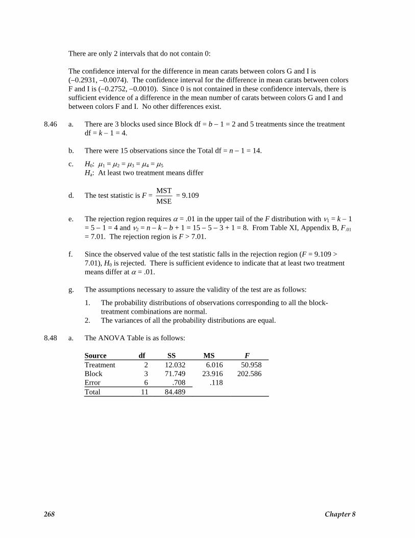
There are only 2 intervals that do not contain 0: The confidence interval for the difference in mean carats between colors G and I is (−0.2931, −0.0074). The confidence interval for the difference in mean carats between colors F and I is (−0.2752, −0.0010). Since 0 is not contained in these confidence intervals, there is sufficient evidence of a difference in the mean number of carats between colors G and I and between colors F and I. No other differences exist.

8.46 a. There are 3 blocks used since Block df = b − 1 = 2 and 5 treatments since the treatment

df = k − 1 = 4. b. There were 15 observations since the Total df = n − 1 = 14.

c. H0: μ1 = μ2 = μ3 = μ4 = μ5

Ha: At least two treatment means differ

d. The test statistic is F = MSEMST = 9.109

e. The rejection region requires α = .01 in the upper tail of the F distribution with ν1 = k − 1

= 5 − 1 = 4 and ν2 = n − k − b + 1 = 15 − 5 − 3 + 1 = 8. From Table XI, Appendix B, F.01 = 7.01. The rejection region is F > 7.01.

f. Since the observed value of the test statistic falls in the rejection region (F = 9.109 >

7.01), H0 is rejected. There is sufficient evidence to indicate that at least two treatment means differ at α = .01.

g. The assumptions necessary to assure the validity of the test are as follows: 1. The probability distributions of observations corresponding to all the block-

treatment combinations are normal. 2. The variances of all the probability distributions are equal. 8.48 a. The ANOVA Table is as follows:

Source df SS MS F Treatment 2 12.032 6.016 50.958 Block 3 71.749 23.916 202.586 Error 6 .708 .118 Total 11 84.489

268 Chapter 8

b. To determine if the treatment means differ, we test: H0: μA = μB = μB C


The test statistic is F = MSEMST = 50.958

The rejection region requires α = .05 in the upper tail of the F distribution with ν1 = k − 1

= 3 − 1 = 2 and ν2 = n − k − b + 1 = 12 − 3 − 4 + 1 = 6. From Table IX, Appendix B, F.05 = 5.14. The rejection region is F > 5.14.

Since the observed value of the test statistic falls in the rejection region (F = 50.958 >

5.14), H0 is rejected. There is sufficient evidence to indicate that the treatment means differ at α = .05.

c. To see if the blocking was effective, we test: H0: μ1 = μ2 = μ3 = μ4

Ha: At least two block means differ

The test statistic is F = MSEMSB = 202.586

The rejection region requires α = .05 in the upper tail of the F distribution with ν1 = k − 1 = 4 − 1 = 3 and ν2 = n − k − b + 1 = 12 − 3 − 4 + 1 = 6. From Table IX, Appendix B, F.05 = 4.76. The rejection region is F > 4.76. Since the observed value of the test statistic falls in the rejection region (F = 202.586 >

4.76), H0 is rejected. There is sufficient evidence to indicate that blocking was effective in reducing the experimental error at α = .05.

d. From the printouts, we are given the differences in the sample means. The difference

between Treatment B and both Treatments A and C are positive (1.125 and 2.450), so Treatment B has the largest sample mean. The difference between Treatment A and C is positive (1.325), so Treatment A has a larger sample mean than Treatment C. So Treatment B has the largest sample mean, Treatment A has the next largest sample mean and Treatment C has the smallest sample mean.

From the printout, all the means are significantly different from each other.

e. The assumptions necessary to assure the validity of the inferences above are:

1. The probability distributions of observations corresponding to all the block-treatment combinations are normal.

2. The variances of all the probability distributions are equal.


8.50 a. This is a randomized block design. The blocks are the 12 plots of land. The treatments are the three methods used on the shrubs: fire, clipping, and control. The response variable is the mean number of flowers produced. The experimental units are the 36 shrubs.

b. Plot c. To determine if there is a difference in the mean number of flowers produced among the

three treatments, we test: H0: μ1 = μ2 = μ3

Ha: The mean number of flowers produced differ for at least two of the methods. The test statistic is F = 5.42 and p = .009. We can reject the null hypothesis at the α > .009 level of significance. At least two of the methods differ with respect to mean

number of flowers produced by pawpaws. d. The means of Control and Clipping do not differ significantly. The means of Clipping

and Burning do not differ significantly. The mean of treatment Burning exceeds that of the Control.

8.52 From the printout, the p-value for treatments or Decoy is p = .589. Since the p-value is not

small, we cannot reject H0. There is insufficient evidence to indicate a difference in mean percentage of a goose flock to approach to within 46 meters of the pit blind among the three decoy types. This conclusion is valid for any reasonable value of α.

270 Chapter 8

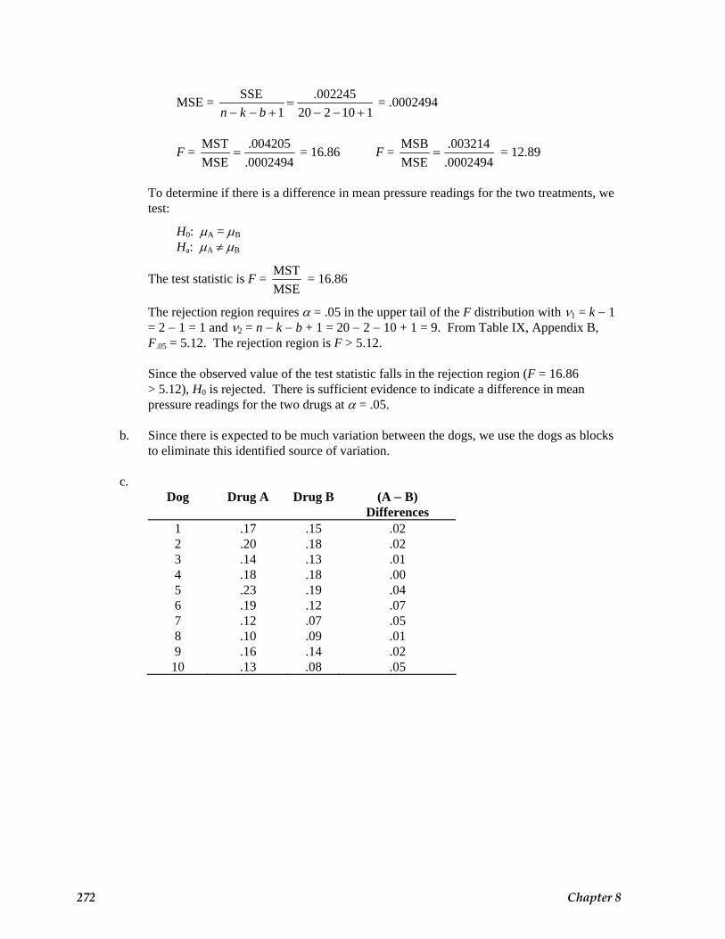
8.54 Using SAS, the ANOVA Table is: The ANOVA Procedure Dependent Variable: temp Sum of Source DF Squares Mean Square F Value Pr > F Model 11 18.53700000 1.68518182 0.52 0.8634 Error 18 58.03800000 3.22433333 Corrected Total 29 76.57500000 R-Square Coeff Var Root MSE temp Mean 0.242076 1.885189 1.795643 95.25000 Source DF Anova SS Mean Square F Value Pr > F STUDENT 9 18.41500000 2.04611111 0.63 0.7537 PLANT 2 0.12200000 0.06100000 0.02 0.9813 To determine if there are differences among the mean temperatures among the three treatments,

we test: H0: μ1 = μ2 = μ3 Ha: At least two treatment means differ The test statistic is F = 0.02. The associated p-value is p = .9813. Since the p-value is very

large, there is no evidence of a difference in mean temperature among the three treatments. Since there is no difference, we do not need to compare the means. It appears that the presence of plants or pictures of plants does not reduce stress.

8.56 a. Some preliminary calculations are:

CM = ( )

1095.2 22

=∑ny

= .435125

SS(Total) = ∑ − CM = .4705 − .435125 = .035375 2y

SST = SS(DRUG) = b

Tb

T 22

21 + − CM =

1033.1

1062.1 22

+ − .435125 = .004205

MST = SST .0042051 2 1k=

− − = .004205, df = k − 1 = 1

SSB = SS(DOG) = 2 2

1 2B Bk k

+ + ⋅⋅⋅ + 2

10Bk

− CM

= 2

21.3.19.19.31.42.36.27.38.32. 2222222222 +++++++++

− .435125 = .028925

MSB = 110

028925.1

SSB−

=−b

= .003214, df = b − 1 = 9

SSE = SS(Total) − SST − SSB = .035375 − .004205 − .028925 = .002245


MSE = SSE .0022451 20 2 10 1n k b=

− − + − − + = .0002494

F = 0002494.004205.

MSEMST

= = 16.86 F = 0002494.003214.

MSEMSB

= = 12.89

To determine if there is a difference in mean pressure readings for the two treatments, we

test: H0: μA = μB B

Ha: μA ≠ μB B

The test statistic is F = MSEMST = 16.86

The rejection region requires α = .05 in the upper tail of the F distribution with ν1 = k − 1

= 2 − 1 = 1 and ν2 = n − k − b + 1 = 20 − 2 − 10 + 1 = 9. From Table IX, Appendix B, F.05 = 5.12. The rejection region is F > 5.12.

Since the observed value of the test statistic falls in the rejection region (F = 16.86

> 5.12), H0 is rejected. There is sufficient evidence to indicate a difference in mean pressure readings for the two drugs at α = .05.

b. Since there is expected to be much variation between the dogs, we use the dogs as blocks

to eliminate this identified source of variation. c.

Dog Drug A Drug B (A − B) Differences

1 .17 .15 .02 2 .20 .18 .02 3 .14 .13 .01 4 .18 .18 .00 5 .23 .19 .04 6 .19 .12 .07 7 .12 .07 .05 8 .10 .09 .01 9 .16 .14 .02

10 .13 .08 .05

272 Chapter 8

Some preliminary calculations are:

.2910

i

d

dd

n= =∑ = .029

( )22

2

2 dd

d

(.29).0129 .00449101 10 1

ii

dd

ns

n

− −= = =

− −

∑∑9

= .0004989

sd = 2d .0004989s = = .02234

To determine if there is a difference in mean pressure readings for the two treatments, we

test: H0: μA = μBB

Ha: μA ≠ μBB

The test statistic is t = d d

0 .029 0/ .02234 / 10

ds n

−=

− = 4.105

The rejection region requires α/2 = .05/2 = .025 in each tail of the t distribution with

df = n − 1 = 10 − 1 = 9. From Table VI, Appendix B, t.025 = 2.262. The rejection region is t < −2.262 or t > 2.262.

Since the observed value of the test statistic falls in the rejection region (t = 4.105

> 2.262), H0 is rejected. There is sufficient evidence to indicate a difference in the treatment means at α = .05.

d. In part a, F = 16.86; and in part c, t = 4.105. Note that t2 = 4.1052 = 16.85 = F. In part a, F.05 = 5.12; and in part c, t.025 = 2.262. Note that = 2.2622

025.t2 = 5.12 = F.05.

e. p-value = P(F ≥ 16.86) with ν1 = 1 and ν2 = 9. Using Table XI, Appendix B, P(F ≥ 10.56) < .01. Thus, the p-value is < .01. The probability of a test statistic this extreme if the treatment means are the same is less

than .01. This is very significant. We would reject H0 in favor of Ha if α is larger than the p-value.

8.58 a. There are two factors. b. No, we cannot tell whether the factors are qualitative or quantitative. c. Yes. There are four levels of factor A and three levels of factor B. d. A treatment would consist of a combination of one level of factor A and one level of

factor B. There are a total of 4 × 3 = 12 treatments.


e. One problem with only one replicate is there are no degrees of freedom for error. This is overcome by having at least two replicates.

8.60 a. Factor A has 3 + 1 = 4 levels and factor B has 1 + 1 = 2 levels. b. There are a total of 23 + 1 = 24 observations and 4 × 2 = 8 treatments. Therefore, there

were 24/8 = 3 observations for each treatment. c. AB df = (a − 1)(b − 1) = (4 − 1)(2 − 1) = 3 Error df = n − ab = 24 − 4(2) = 16

MSA = SS 1

Aa −

⇒ SSA = (a − 1)MSA = (4 − 1)(.75) = 2.25

MSB = SS .95 1 2 1

Bb

=− −

= .95

MSAB = SS( 1)( 1)

ABa b− −

⇒ SSAB = (a − 1)(b − 1)MSAB = (4 − 1)(2 − 1)(.30) = .9

SSE = SS(Total) − SSA − SSB − SSAB = 6.5 − 2.25 − .95 − .9 = 2.4

MSE = SSE 2.4 24 - 4(2)n ab

=−

= .15

SST = SSA + SSB + SSAB = 2.25 + .95 + .90 = 4.1 Treatment df = ab − 1 = 4(2) − 1 = 7

MST = SST 4.1 1 7ab

=−

= .5857 FT = MST .5857 MSE .15

= = 3.90

FA = MSA .75 = = 5.00MSE .15

FB = B 6.33 = .15.95 =

MSEBMS

FAB = MSAB .30 = = 2.00MSE .15

The ANOVA table is:

Source df SS MS FTreatments 7 4.1 .59 3.90A 3 2.25 .75 5.00 B 1 .95 .95 6.33 AB 3 .90 .30 2.00 Error 16 2.40 .15 Total 23 6.50

274 Chapter 8

d. To determine whether the treatment means differ, we test: H0: μ1 = μ2 = ⋅⋅⋅ = μ8


The test statistic is F = MSTMSE

= 3.90

The rejection region requires α = .10 in the upper tail of the F-distribution with ν1 = ab −

1 = 4(2) − 1 = 7 and ν2 = n − ab = 24 − 4(2) = 16. From Table VIII, Appendix B, F.10 = 2.13. The rejection region is F > 2.13.


H0 is rejected. There is sufficient evidence to indicate the treatment means differ at α = .10.

e. To determine if the factors interact, we test: H0: Factors A and B do not interact to affect the response mean Ha: Factors A and B do interact to affect the response mean The test statistic is F = 2.00. The rejection region requires α = .10 in the upper tail of the F-distribution with ν1 =

(a − 1)(b − 1) = (4 − 1)(2 − 1) = 3 and ν2 = n − ab = 24 − 4(2) = 16. From Table VIII, Appendix B, F.10 = 2.46. The rejection region is F > 2.46.


>/ 2.46), H0 is not rejected. There is insufficient evidence to indicate factors A and B interact at α = .10.

To determine if the four means of factor A differ, we test: H0: There is no difference in the four means of factor A Ha: At least two of the factor A means differ The test statistic is F = 5.00. The rejection region requires α = .10 in the upper tail of the F-distribution with ν1 =

a − 1 = 4 − 1 = 3 and ν2 = n − ab = 24 - 4(2) = 16. From Table VIII, Appendix B, F.10 = 2.46. The rejection region is F > 2.46.


H0 is rejected. There is sufficient evidence to indicate at least two of the four means of factor A differ at α = .10.

To determine if the 2 means of factor B differ, we test: H0: There is no difference in the two means of factor B Ha: At least two of the factor B means differ


The test statistic is F = 6.33. The rejection region requires α = .10 in the upper tail of the F-distribution with ν1 =

b − 1 = 2 − 1 = 1 and ν2 = n − ab = 24 − 4(2) = 16. From Table VIII, Appendix B, F.10 = 3.05. The rejection region is F > 3.05.


H0 is rejected. There is sufficient evidence to indicate the two means of factor B differ at α = .10.

All of the tests performed are warranted because interaction was not significant. 8.62 a. The treatments are the combinations of the levels of factor A and the levels of factor B.

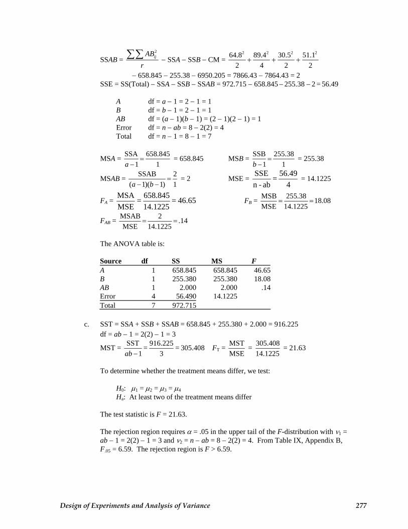
There are 2 × 2 = 4 treatments. The treatment means are:

1111

29.6 35.22 2x

x += =∑ = 32.4 12

1247.3 42.1

2 2x

x += =∑

2121

12.9 17.62 2x

x += =∑ = 15.25 22

2228.4 22.7

2 2x

x += =∑

The factors do not appear to interact—the

lines are almost parallel. The treatment means do appear to differ because the sample means range from 15.25 to 44.7.

b. CM = ( )2

2235.88

ix

n=

∑

SS(Total) = 2x∑ − CM = 7922.92 − 6950.205 = 972.715

SSA = 2 2 2154.2 81.6CM=

2(2) 2(2)iA

br− +∑ = 7609.05 − 6950.205 = 658.845

SSB = 2 2 295.3 140.5CM=

2(2) 2(2)iB

ar− +∑ = 7205.585 − 6950.205 = 255.38

276 Chapter 8

SSAB = 2ijAB

r∑∑ − SSA − SSB − CM =

2 2 264.8 89.4 30.5 51.12 4 2 2

+ + +2

− 658.845 − 255.38 − 6950.205 = 7866.43 − 7864.43 = 2 SSE = SS(Total) − SSA − SSB − SSAB = 972.715 − 658.845 − 255.38 − 2 = 56.49 A df = a − 1 = 2 − 1 = 1 B df = b − 1 = 2 − 1 = 1 AB df = (a − 1)(b − 1) = (2 − 1)(2 − 1) = 1 Error df = n − ab = 8 − 2(2) = 4 Total df = n − 1 = 8 − 1 = 7

MSA = SSA 658.845 1 1a

=−

= 658.845 MSB = SSB 255.38 1 1b=

− = 255.38

MSAB = SSAB 2 ( 1)( 1) 1a b

=− −

= 2 MSE = 4

56.49 = ab-n

SSE = 14.1225

FA = 46.65 = 14.1225658.845 =

MSEAMS

FB = B

MSB 255.38 18.08MSE 14.1225

= =

FAB = MSAB 2 .14MSE 14.1225

= =

The ANOVA table is:

Source df SS MS F A 1 658.845 658.845 46.65 B 1 255.380 255.380 18.08 AB 1 2.000 2.000 .14 Error 4 56.490 14.1225 Total 7 972.715

c. SST = SSA + SSB + SSAB = 658.845 + 255.380 + 2.000 = 916.225 df = ab − 1 = 2(2) − 1 = 3

MST = SST 916.225 = = 305.408 1 3ab −

FT = MST 305.408 = MSE 14.1225

= 21.63

To determine whether the treatment means differ, we test: H0: μ1 = μ2 = μ3 = μ4

Ha: At least two of the treatment means differ The test statistic is F = 21.63. The rejection region requires α = .05 in the upper tail of the F-distribution with ν1 =

ab − 1 = 2(2) − 1 = 3 and ν2 = n − ab = 8 − 2(2) = 4. From Table IX, Appendix B, F.05 = 6.59. The rejection region is F > 6.59.


Since the observed value of the test statistic falls in the rejection region (F = 21.63 > 6.59), H0 is rejected. There is sufficient evidence to indicate the treatment means differ at α = .05.

This agrees with the conclusion in part a. d. Since there are differences among the treatment means, we test for the presence of

interaction: H0: Factors A and B do not interact to affect the response means Ha: Factors A and B do interact to affect the response means The test statistic is F = .14. The rejection region requires α = .05 in the upper tail of the F-distribution with ν1 =

(a − 1)(b − 1) = (2 − 1)(2 − 1) = 1 and ν2 = n − ab = 8 − 2(2) = 4. From Table IX, Appendix B, F.05 = 7.71. The rejection region is F > 7.71.

Since the observed value of the test statistic does not fall in the rejection region (F = .14

>/ 7.71), H0 is not rejected. There is insufficient evidence to indicate the factors interact at α = .05.

e. Since the interaction was not significant, we test for main effects. To determine whether the two means of factor A differ, we test: H0: μ1 = μ2

Ha: μ1 ≠ μ2 The test statistic is F = 46.65. The rejection region requires α = .05 in the upper tail of the F-distribution with ν1 =

a − 1 = 2 − 1 = 1 and ν2 = n − ab = 8 − 2(2) = 4. From Table IX, Appendix B, F.05 = 7.71. The rejection region is F > 7.71.


7.71), H0 is rejected. There is sufficient evidence to indicate the two means of factor A differ at α = .05.

To determine whether the two means of factor B differ, we test: H0: μ1 = μ2

Ha: μ1 ≠ μ2 The test statistic is F = 18.08. The rejection region requires α = .05 in the upper tail of the F-distribution with ν1 = b − 1

= 2 − 1 = 1 and ν2 = n − ab = 8 − 2(2) = 4. From Table IX, Appendix B, F.05 = 7.71. The rejection region is F > 7.71.

278 Chapter 8

Since the observed value of the test statistic falls in the rejection region (F = 18.08 > 7.71), H0 is rejected. There is sufficient evidence to indicate the two means of factor B differ at α = .05.

f. The results of all the tests agree with those in part a. g. Since no interaction is present, but the means of both factors A and B differ, we compare

the two means of factor A and compare the two means of factor B. Since there are only two means to compare for each factor, the higher population mean corresponds to the higher sample mean.

Factor A: 11

29.6 35.2 47.3 42.12(2)

xx

br+ + +

= =∑ = 38.55

22

12.9 17.6 28.4 22.72(2)

xx

br+ + +

= =∑ = 20.4

The mean for level 1 of factor A is significantly higher than the mean for level 2.

Factor B: 11

29.6 35.2 12.9 17.62(2)

xx

ar+ + +

= =∑ = 23.825

22

47.3 42.1 28.4 22.72(2)

xx

ar+ + +

= =∑ = 35.125

The mean for level 2 of factor B is significantly higher than the mean for level 1. 8.64 a. There are a total of 2 × 4 = 8 treatments.

b. The interaction between temperature and type was significant. This means that the effect of type of yeast on the mean autolysis yield depends on the level of temperature.

c. To determine if the main effect of type of yeast is significant, we test:

H0: μBa = μBr

Ha: μBa ≠ μBr

To determine if the main effect of temperature is significant, we test: H0: μ1 = μ2 = μ3 = μ4

Ha: At least one mean differs

d. The tests for the main effects should not be run until after the test for interaction is conducted. If interaction is significant, then these interaction effects could cover up the main effects. Thus, the main effect tests would not be informative.

If the test for interaction is not significant, then the main effect tests could be run.


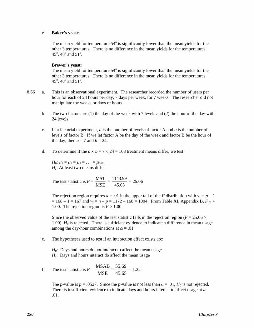
e. Baker’s yeast: The mean yield for temperature 54o is significantly lower than the mean yields for the other 3 temperatures. There is no difference in the mean yields for the temperatures 45o, 48o and 51o. Brewer’s yeast: The mean yield for temperature 54o is significantly lower than the mean yields for the other 3 temperatures. There is no difference in the mean yields for the temperatures 45o, 48o and 51o. 8.66 a. This is an observational experiment. The researcher recorded the number of users per hour for each of 24 hours per day, 7 days per week, for 7 weeks. The researcher did not

manipulate the weeks or days or hours. b. The two factors are (1) the day of the week with 7 levels and (2) the hour of the day with 24 levels. c. In a factorial experiment, a is the number of levels of factor A and b is the number of

levels of factor B. If we let factor A be the day of the week and factor B be the hour of the day, then a = 7 and b = 24.

d. To determine if the a × b = 7 × 24 = 168 treatment means differ, we test: H0: μ1 = μ2 = μ3 = . . . = μ168 Ha: At least two means differ

The test statistic is F = MST 1143.99 = MSE 45.65

= 25.06

The rejection region requires α = .01 in the upper tail of the F distribution with v1 = p − 1

= 168 − 1 = 167 and v2 = n − p = 1172 – 168 = 1004. From Table XI, Appendix B, F.01 ≈ 1.00. The rejection region is F > 1.00.


1.00), H0 is rejected. There is sufficient evidence to indicate a difference in mean usage among the day-hour combinations at α = .01.

e. The hypotheses used to test if an interaction effect exists are: H0: Days and hours do not interact to affect the mean usage Ha: Days and hours interact do affect the mean usage

f. The test statistic is F = 45.6555.69 =

MSEMSAB

= 1.22

The p-value is p = .0527. Since the p-value is not less than α = .01, H0 is not rejected.

There is insufficient evidence to indicate days and hours interact to affect usage at α = .01.

280 Chapter 8

g. To determine if the mean usage differs among the days of the week, we test: H0: μ1 = μ2 = μ3 = μ4 = μ5 = μ6 = μ7


The test statistic is F = 45.65

3122.02 = MSEMSA

= 68.39

The p-value is p = .0001. Since the p-value is less than α = .01, H0 is rejected. There is

sufficient evidence to indicate the mean usage differs among the days of the week at α = .01.

To determine if the mean usage differs among the hours of the day, we test: H0: μ1 = μ2 = μ3 = . . . = μ24 Ha: At least two means differ

The test statistic is F = 45.65

7157.82 = MSEMSB

= 156.80

The p-value is p = .0001. Since the p-value is less than α = .01, H0 is rejected. There is

sufficient evidence to indicate the mean usage differs among the hours of the day at α = .01.

8.68 a. The degrees of freedom for “Type of message retrieval system” is a − 1 = 2 − 1 = 1. The

degrees of freedom for “Pricing option” is b − 1 = 2 − 1 = 1. The degrees of freedom for the interaction of Type of message retrieval system and Pricing option is (a − 1)(b – 1) = (2 − 1)(2 − 1) = 1. The degrees of freedom for error is n − ab = 120 − 2(2) = 116.

Source Df SS MS F Type of message retrieval system 1 - - 2.001 Pricing Option 1 - - 5.019 Type of system × pricing option 1 - - 4.986 Error 116 - - Total 119

b. To determine if “Type of system” and “Pricing option” interact to affect the mean

willingness to buy, we test: H0: “Type of system” and “Pricing option” do not interact Ha: “Type of system” and “Pricing option” interact

c. The test statistic is F = MSE

MSAB = 4.986

The rejection region requires α = .05 in the upper tail of the F distribution with ν1 = (a − 1)(b − 1) = (2 − 1)(2 − 1) = 1 and ν2 = n − ab = 120 − 2(2) = 116. From Table IX,

Appendix B, F.05 ≈ 3.92. The rejection region is F > 3.92.


Since the observed value of the test statistic falls in the rejection region (F = 4.986 > 3.92), H0 is rejected. There is sufficient evidence to indicate “Type of system” and “Pricing option” interact to affect the mean willingness to buy at α = .05.

d. No. Since the test in part c indicated that interaction between “Type of system” and

“Pricing option” is present, we should not test for the main effects. Instead, we should proceed directly to a multiple comparison procedure to compare selected treatment means. If interaction is present, it can cover up the main effects.

8.70 a. The treatments are the 3 × 3 = 9 combinations of PES and Trust. The nine treatments are:

(BC, Low), (PC, Low), (NA, Low), (BC, Med), (PC, Med), (NA, Med), (BC, High), (PC, High), and (NA, High).

b. df(Trust) = 3 − 1 = 2; SSE = SSTot − SS(PES) − SS(Trust) − SSPT = 161.1162 − 2.1774 − 7.6367 − 1.7380 = 149.5641

MS(PES) = SS(PES)df(PES)

= 2.17742

= 1.0887

MS(Trust) = SS(Trust)df(Trust)

= 7.63672

= 3.81835

MS(PT) = SS(PT)df(PT)

= 1.73804

= 0.4345

MSE = SSEdf(Error)

= 149.5641206

= 0.7260

FPES = MS(PES)MSE

= 1.08870.7260

= 1.50 FTrust = MS(Trust)MSE

= 3.818350.7260

= 5.26

FPT = MS(PT)MSE

= 0.43450.7260

= 0.60

The ANOVA table is:

Source df SS MS F PES 2 2.1774 1.0887 1.50Trust 2 7.6367 3.81835 5.26PES × Trust 4 1.7380 0.4345 0.60Error 206 149.5641 0.7260Total 214 161.1162

c. To determine if PES and Trust interact, we test: H0: PES and Trust do not interact to affect the mean tension Ha: PES and Trust do interact to affect the mean tension The test statistic is F = 0.60.

282 Chapter 8

The rejection region requires α = .05 in the upper tail of the F-distribution with ν1 = (a − 1)(b − 1) = (3 − 1)(3 − 1) = 4 and ν2 = n − ab = 215 − 3(3) = 206. From Table IX, Appendix B, F.05 ≈ 2.37. The rejection region is F > 2.37.


>/ 2.37), H0 is not rejected. There is insufficient evidence to indicate that PES and Trust interact at α = .05.

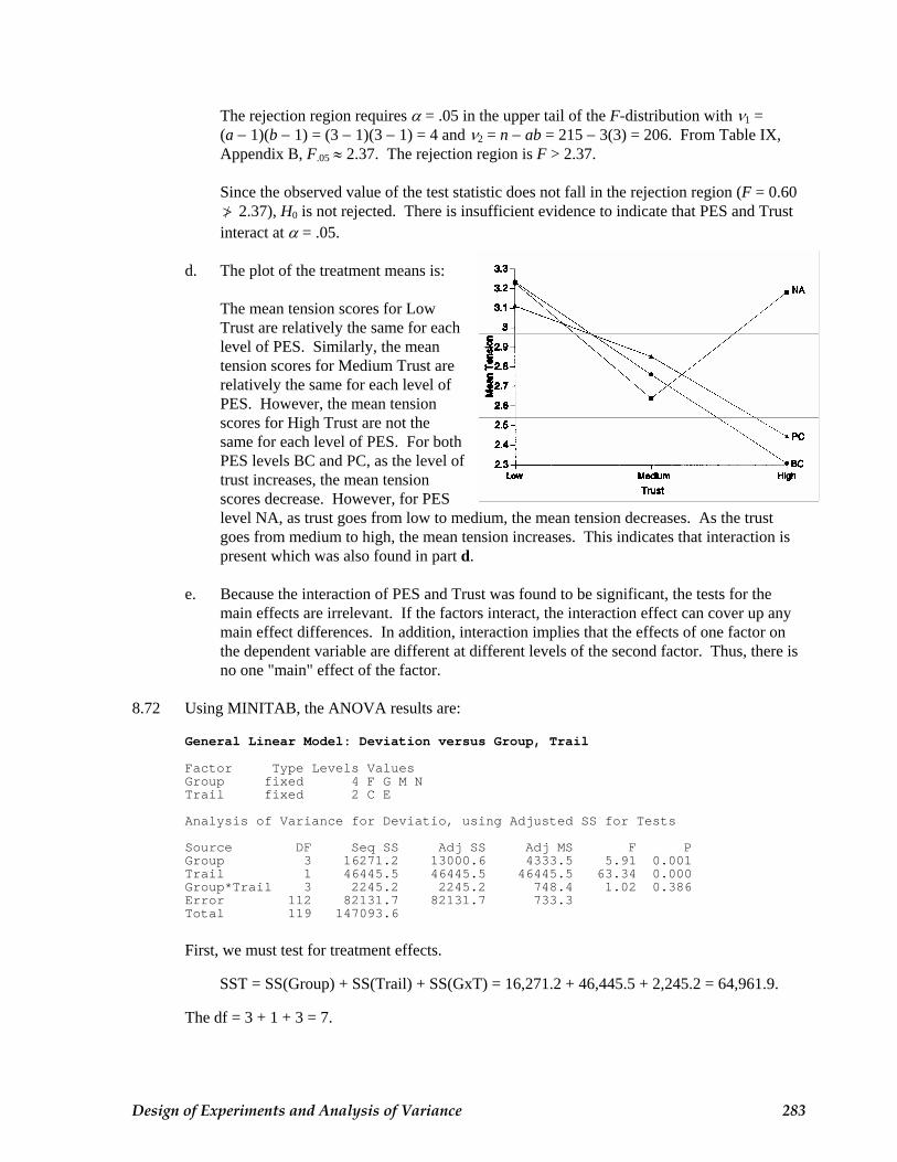
d. The plot of the treatment means is: The mean tension scores for Low

Trust are relatively the same for each level of PES. Similarly, the mean tension scores for Medium Trust are relatively the same for each level of PES. However, the mean tension scores for High Trust are not the same for each level of PES. For both PES levels BC and PC, as the level of trust increases, the mean tension scores decrease. However, for PES level NA, as trust goes from low to medium, the mean tension decreases. As the trust goes from medium to high, the mean tension increases. This indicates that interaction is present which was also found in part d.

e. Because the interaction of PES and Trust was found to be significant, the tests for the

main effects are irrelevant. If the factors interact, the interaction effect can cover up any main effect differences. In addition, interaction implies that the effects of one factor on the dependent variable are different at different levels of the second factor. Thus, there is no one "main" effect of the factor.

8.72 Using MINITAB, the ANOVA results are:

General Linear Model: Deviation versus Group, Trail

Factor Type Levels Values Group fixed 4 F G M N Trail fixed 2 C E

Analysis of Variance for Deviatio, using Adjusted SS for Tests

Source DF Seq SS Adj SS Adj MS F P Group 3 16271.2 13000.6 4333.5 5.91 0.001 Trail 1 46445.5 46445.5 46445.5 63.34 0.000 Group*Trail 3 2245.2 2245.2 748.4 1.02 0.386 Error 112 82131.7 82131.7 733.3 Total 119 147093.6 First, we must test for treatment effects.

SST = SS(Group) + SS(Trail) + SS(GxT) = 16,271.2 + 46,445.5 + 2,245.2 = 64,961.9.

The df = 3 + 1 + 3 = 7.


SST 64,961.9MST 9, 280.27141 4(2) 1ab

= = =− −

MST 9, 280.2714F= 12.66MSE 733.3

= =

To determine if there are differences in mean ratings among the 8 treatments, we test: H0: All treatment means are the same Ha: At least two treatment means differ The test statistic is F = 12.66.

Since no α was given, we will use α = .05. The rejection region requires α = .05 in the upper tail of the F distribution with ν1 = ab – 1 = 4(2) – 1 = 7 and ν2 = n – ab = 120 – 4(2) = 112. From Table IX, Appendix B, F.05 ≈ 2.09. The rejection region is F > 2.09. Since the observed value of the test statistic falls in the rejection region (F = 12.66 > 2.09), H0 is rejected. There is sufficient evidence that differences exist among the treatment means at α = .05. Since differences exist, we now test for the interaction effect between Trail and Group. To determine if Trail and Group interact, we test: H0: Trail and Group do not interact Ha: Trail and Group do interact The test statistic is F = 1.02 and p = .386 Since the p-value is greater than α (p = .386 > .05), H0 is not rejected. There is insufficient evidence that Trail and Group interact at α = .05. Since the interaction does not exist, we test for the main effects of Trail and Group. To determine if there are differences in the mean rating between the two levels of Trail, we test: H0: μ1 = μ2 Ha: μ1 ≠ μ2 The test statistics is F = 63.34 and p = 0.000. Since the p-value is greater than α (p = .000 < .05), H0 is rejected. There is sufficient evidence that the mean trail deviations differ between the fecal extract trail and the control trail α = .05. To determine if there are differences in the mean rating between the four levels of Group, we test: H0: μ1 = μ2 = μ3 = μ4

Ha: At least 2 means differ The test statistics is F = 5.91 and p = 0.001. Since the p-value is less than α (p = 0.001 < .05), Ho is rejected. There is sufficient evidence that the mean trail deviations differ among the four groups at α = .05.

284 Chapter 8

8.74 There are 3 × 2 = 6 treatments. They are A1BB1, A1B2B , A2BB1, A2B2B , A3BB1, and A3B2B . 8.76 a. SSE = SSTot − SST = 62.55 − 36.95 = 25.60 df Treatment = p − 1 = 4 − 1 = 3 df Error = n − p = 20 − 4 = 16 df Total = n − 1 = 20 − 1 = 19

MST = SST/df = 36.953

= 12.32

MSE = SSE/df = 25.6016

= 1.60

F = MSTMSE

= 12.321.60

= 7.70

The ANOVA table:

Source df SS MS F Treatment 3 36.95 12.32 7.70 Error 16 25.60 1.60 Total 19 62.55

b. To determine if there is a difference in the treatment means, we test: H0: μ1 = μ2 = μ3 = μ4

Ha: At least two of the means differ where the μi represents the mean for the ith treatment.

The test statistic is F = MSEMST

= 7.70

The rejection region requires α = .10 in the upper tail of the F-distribution with ν1 = (p − 1) = (4 − 1) = 3 and ν2 = (n − p) = (20 − 4) = 16. From Table VIII, Appendix B,

F.10 = 2.46. The rejection region is F > 2.46. Since the observed value of the test statistic falls in the rejection region (F = 7.70 > 2.46),

H0 is rejected. There is sufficient evidence to conclude that at least two of the means differ at α = .10.

c. 4x = 4

4

575

xn

=∑ = 11.4

For confidence level .90, α = .10 and α/2 = .10/2 = .05. From Table VI, Appendix B,

with df = 16, t.05 = 1.746. The confidence interval is: 4x ± .05 4MSE/t n ⇒ 11.4 ± 1.746⋅ 1.6 /5 ⇒ 11.4 ± .99 ⇒ (10.41, 12.39)


8.78 a. df(AB) = (a − 1)(b - 1) = 3(5) = 15 df(Error) = n − ab = 48 − 4(6) = 24 SSAB = MSAB(df) = 3.1(15) = 46.5 SS(Total) = SSA + SSB + SSAB + SSE = 2.6 + 9.2 + 46.5 + 18.7 = 77

MSA = SS 2.6 .8667 1 3

Aa

= =−

MSB = SS 9.2 1.84 1 5B

b= =

−

MSE = SSE 18.7 .7792 24n ab

= =−

FA = MSA .8667 1.11MSE .7792

= = FB = B

MSB 1.84 2.36MSE .7792

= =

FAB = MS 3.1 3.98MSE .7792

AB= =

Source df SS MS F A 3 2.6 .8667 1.11B 5 9.2 1.84 2.36AB 15 46.5 3.1 3.98Error 24 18.7 .7792 Total 47 77.0

b. Factor A has a = 3 + 1 = 4 levels and factor B has b = 5 + 1 = 6 levels. The number of

treatments is ab = 4(6) = 24. The total number of observations is n = 47 + 1 = 48. Thus, two replicates were performed.

c. SST = SSA + SSB + SSAB = 2.6 + 9.2 + 46.5 = 58.3

MST = SST 58.3 2.5347 1 4(6) 1ab

= =− −

F = MST 2.5347 3.25MSE .7792

= =

To determine whether the treatment means differ, we test: H0: μ1 = μ2 = ⋅⋅⋅ = μ24

Ha: At least one treatment mean is different


= 3.25

The rejection region requires α = .05 in the upper tail of the F-distribution with ν1 = ab −

1 = 4(6) − 1 = 23 and ν2 = n − ab = 48 - 4(6) = 24. From Table IX, Appendix B, F.05 ≈ 2.03. The rejection region is F > 2.03.


H0 is rejected. There is sufficient evidence to indicate the treatment means differ at α = .05.

286 Chapter 8

d. Since there are differences among the treatment means, we test for the presence of interaction:

H0: Factor A and factor B do not interact to affect the response mean Ha: Factor A and factor B do interact to affect the response mean

The test statistic is F = MSMSE

AB = 3.98

The rejection region requires α = .05 in the upper tail of the F-distribution with ν1 =

(a − 1)(b − 1) = (4 − 1)(6 − 1) = 15 and ν2 = n − ab = 48 − 4(6) = 24. From Table IX, Appendix B, F.05 = 2.11. The rejection region is F > 2.11.


H0 is rejected. There is sufficient evidence to indicate factors A and B interact to affect the response means at α = .05.

Since the interaction is significant, no further tests are warranted. Multiple comparisons

need to be performed. 8.80 a. This is a two-factor factorial design. It is also a completely randomized design. b. The two factors are "involvement in topic" and "question wording." Both are qualitative

variables because neither are measured on numerical scales. c. There are two levels of "involvement in topic": high and low. There are two levels of

"question wording": positive and negative. d. There are 2 × 2 = 4 treatments. The are: (high, positive), (high, negative), (low, positive), and (low, negative) e. The experiment's dependent variable is the level of agreement. 8.82 a. To determine if the mean vacancy rates of the eight office-property submarkets in Atlanta differ, we test: H0: μ1 = μ2 = μ3 = μ4 = μ5 = μ6 = μ7 = μ8

Ha: At least two means differ b. If quarterly data were used for nine years, there are 4 × 9 = 36 observations per

submarket. Since there are 8 submarkets, the total sample size is 8 × 36 = 288. Since no value of α is given, we will use α = .05.

The rejection region requires α = .05 in the upper tail of the F-distribution with ν1 = k − 1

= 8 − 1 = 7 and ν2 = n − k = 288 – 8 = 280. From Table X, Appendix B, F.05 ≈ 2.01. The rejection region is F > 2.01.


Since the observed value of the test statistic falls in the rejection region (F = 17.54 > 2.01), H0 is rejected. There is sufficient evidence to indicate the mean vacancy rates of the eight office-property submarkets in Atlanta differ at α = .05.

c. With ν1 = k − 1 = 8 − 1 = 7 and ν2 = n − k = 288 – 8 = 280, P(F > 17.54) < .01, using

Table XI, Appendix B. Thus, the p-value is less than .01. d. We must assume that all eight samples are randomly drawn from normal populations, the

eight populations variances are the same, and the samples are independent. e. The mean vacancy rate for the South submarket is significantly larger than the mean

vacancy rates for all other submarkets. The mean vacancy rate of the Downtown submarket is significantly larger than the mean vacancy rates for all other submarkets except the South. The mean vacancy rate of the North Lake submarket is significantly larger than the mean vacancy rates for all other submarkets except the South and Downtown. The mean vacancy rate of the Midtown submarket is significantly larger than the mean vacancy rates for all other submarkets except the South, Downtown, and North Lake. There are no other significant differences.

8.84 a. The response is the weight of a brochure. There is one factor and it is carton. The

treatments are the five different cartons, while the experimental units are the brochures.

b. CM = ( )2

2.7500540

y

n=

∑ = .01406437506

SS(Total) = − CM = .014066537 − .01406437506 = .00000216264 2y∑ SST =

2i

i

Tn∑ − CM =

2 2 2 2. . . . .14767 15028 14962 15217 150318 8 8 8 8

+ + + +2

− .01406437506

= .01406568209 - .01406437506 = .00000130703 SSE = SS(Total) − SST = .00000216264 - .00000130703 = .00000085561

MST = SST .00000130703 1 5 1k

=− −

= .000000326756

MSE = SSE .00000085561 40 5n k

=− −

= .000000024446

F = MST .000000326756 MSE .000000024446

= = 13.37

Source df SS MS F Treatments 4 .00000130703 .000000326756 13.37Error 35 .00000085561 .000000024446Total 39 .00000216264

To determine whether there are differences in mean weight per brochure among the five

cartons, we test: H0: μ1 = μ2 = μ3 = μ4 = μ5


288 Chapter 8

The test statistic is F = 13.37. The rejection region requires α = .05 in the upper tail of the F-distribution with ν1 = k − 1



2.53), H0 is rejected. There is sufficient evidence to indicate a difference in mean weight per brochure among the five cartons at α = .05.

c. We must assume that the distributions of weights for the brochures in the five cartons are

normal, that the variances of the weights for the brochures in the five cartons are equal, and that random and independent samples were selected from each of the cartons.

d. Using MINITAB, the results of Tukey’s multiple comparison procedure are: Individual 95% CIs For Mean Based on Pooled StDev Level N Mean StDev ---+---------+---------+---------+----- Carton1 8 0.018459 0.000105 (-----*-----) Carton2 8 0.018785 0.000101 (----*-----) Carton3 8 0.018703 0.000109 (----*-----) Carton4 8 0.019021 0.000232 (-----*-----) Carton5 8 0.018789 0.000188 (----*-----) ---+---------+---------+---------+------ 0.01840 0.01860 0.01880 0.01900 Pooled StDev = 0.000156 Tukey 95% Simultaneous Confidence Intervals All Pairwise Comparisons Individual confidence level = 99.32% Carton1 subtracted from: Lower Center Upper Carton2 0.0001013 0.0003262 0.0005512 Carton3 0.0000188 0.0002437 0.0004687 Carton4 0.0003375 0.0005625 0.0007875 Carton5 0.0001050 0.0003300 0.0005550 ------+---------+---------+---------+--- Carton2 (-----*------) Carton3 (-----*-----) Carton4 (-----*-----) Carton5 (-----*------) ------+---------+---------+---------+--- -0.00035 0.00000 0.00035 0.00070 Carton2 subtracted from: Lower Center Upper Carton3 -0.0003075 -0.0000825 0.0001425 Carton4 0.0000113 0.0002363 0.0004612 Carton5 -0.0002212 0.0000037 0.0002287 ------+---------+---------+---------+--- Carton3 (------*-----) Carton4 (------*-----) Carton5 (-----*------) ------+---------+---------+---------+--- -0.00035 0.00000 0.00035 0.00070


Carton3 subtracted from: Lower Center Upper Carton4 0.0000938 0.0003187 0.0005437 Carton5 -0.0001387 0.0000862 0.0003112 ------+---------+---------+---------+--- Carton4 (-----*------) Carton5 (-----*------) ------+---------+---------+---------+--- -0.00035 0.00000 0.00035 0.00070 Carton4 subtracted from: Lower Center Upper Carton5 -0.0004575 -0.0002325 -0.0000075 ------+---------+---------+---------+--- Carton5 (-----*------) ------+---------+---------+---------+--- -0.00035 0.00000 0.00035 0.00070 The means arranged in order are: Carton 1 Carton 3 Carton 2 Carton 5 Carton 4 .018459 .018703 .018785 .018789 .019021 The interpretation of the Tukey results are: The mean weight for carton 4 is significantly higher than the mean weights of all the other cartons. The mean weights of cartons 5, 4, and 3 are significantly higher than the mean weight of carton 1. e. Since there are differences among the cartons, management should sample from many

cartons. 8

.86 a. This is a randomized block design.

Response: the length of time required for a cut to stop bleeding Factor: drug Factor type: qualitative Treatments: drugs A, B, and C Experimental units: subjects

290 Chapter 8

b. Using MINITAB, the results are:

General Linear Model: Y versus Drug, Person

Factor Type Levels Values Drug fixed 3 A B C Person fixed 5 1 2 3 4 5

Analysis of Variance for Y, using Adjusted SS for Tests

Source DF Seq SS Adj SS Adj MS F P Drug 2 156.4 156.4 78.2 3.91 0.066 Person 4 7645.8 7645.8 1911.5 95.51 0.000 Error 8 160.1 160.1 20.0 Total 14 7962.3

Tukey 90.0% Simultaneous Confidence Intervals Response Variable Y All Pairwise Comparisons among Levels of Drug

Drug = A subtracted from:

Drug Lower Center Upper -----+---------+---------+---------+- B -11.56 -4.820 1.922 (-------*-------) C -3.72 3.020 9.762 (--------*-------) -----+---------+---------+---------+- -8.0 0.0 8.0 16.0

Drug = B subtracted from:

Drug Lower Center Upper -----+---------+---------+---------+- C 1.098 7.840 14.58 (--------*-------) -----+---------+---------+---------+- -8.0 0.0 8.0 16.0

Let μ1, μ2, and μ3 represent the mean clotting time for the three drugs.

H0: μ1 = μ2 = μ3 Ha: At least two means differ

The test statistic is F = MSE

MS(Drug) = 3.91

The p-value is p = 0.066. Since the observed level of significance is less than α = .10, H0 is rejected. There is sufficient evidence to indicate differences in the mean clotting times among the three drugs at α = .10.

c. The observed level of significance is given as 0.066. d. To determine if there is a significant difference in the mean response over blocks, we test: H0: μ1 = μ2 = μ3 = μ4 = μ5

Ha: At least two block means differ

The test statistic is F = MSE

MS(Person) = 95.51


The p-value is p = 0.000. Since the observed level of significance is less than α = .10, H0 is rejected. There is sufficient evidence to indicate differences in the mean clotting times among the five people at α = .10.

e. The confidence interval to compare drugs A and B is (-11.56, 1.922). Since 0 is in the

interval, there is no evidence of a difference in mean clotting times between drugs A and B.

The confidence interval to compare drugs A and C is (-3.72, 9.762). Since 0 is in the interval, there is no evidence of a difference in mean clotting times between drugs A and C. The confidence interval to compare drugs B and C is (1.098, 14.58). Since 0 is not in the interval, there is evidence of a difference in mean clotting times between drugs B and C. Since the numbers are positive, the mean clotting time for drug C is greater than that for drug B. In summary, the mean clotting time for drug C is greater than that for drug B. No other differences exist.

8.88 a. MSA = SS

A

Adf

= 243.21

= 243.2 MSB = SS

B

Bdf

= 57.81

= 57.8

SSAB = SSTot- SSA - SSB - SSE = 976.3 - 243.2 - 57.8 - 670.8 = 4.5

MSAB = SS

AB

ABdf

= 4.51

= 4.5 MSE = SSE

Edf = 670.8

77 = 8.712

FA = MSMSE

A = 243.28.712

= 27.92 FB = B

MSEBMS

= 57.88.712

= 6.63

FAB = MSE

ABMS = 4.5

8.712 = 0.52

The ANOVA table is:

Source df SS MS F Recent Performance (A) 1 243.2 243.2 27.92Risk attitude(B) 1 57.8 57.8 6.63AB 1 4.5 4.5 0.52Error 77 670.8 8.712 Total 80 976.3

b. To determine if factors A and B interact, we test: H0: Factors A and B do not interact to affect the mean decision Ha: Factors A and B do interact to affect the mean decision The test statistic is F = 0.52.

292 Chapter 8

The rejection region requires α = .05 in the upper tail of the F-distribution with ν1 = (a − 1)(b − 1) = (2 − 1)(2 − 1) = 1 and ν2 = n − ab = 81 − 2(2) = 77. From Table IX, Appendix B, F.05 ≈ 4.00. The rejection region is F > 4.00.

Since the observed value of the test statistic does not fall in the rejection region (F = .52

>/ 4.00), H0 is not rejected. There is insufficient evidence to indicate that factors A and B interact at α = .05.

c. Since the interaction is not significant, the main effect tests are meaningful. To determine if an individual's risk attitude affects his or her budgetary decisions, we test: H0: No difference exists between the risk attitude means Ha: The risk attitude means differ The test statistic is F = 6.63. The rejection region requires α = .05 in the upper tail of the F-distribution with ν1 = b − 1

= 2 − 1 = 1 and ν2 = n − ab = 81 − 2(2) = 77. From Table IX, Appendix B, F.05 ≈ 4.00. The rejection region is F > 4.00.


H0 is rejected. There is sufficient evidence to indicate an individual's risk attitude affects his or her budgetary decisions at α = .05.

d. To determine if recent performance affects budgeting decisions, we test: H0: No difference exists between the recent performance means Ha: The recent performance means differ The test statistic is F = 27.92. The rejection region requires α = .01 in the upper tail of the F-distribution with ν1 = a − 1

= 2 − 1 = 1 and ν2 = n − ab = 81 − 2(2) = 77. From Table XI, Appendix B, F.01 ≈ 7.08. The rejection region is F > 7.08.


7.08), H0 is rejected. There is sufficient evidence to indicate that recent performance affects his or her budgetary decisions at α = .01.


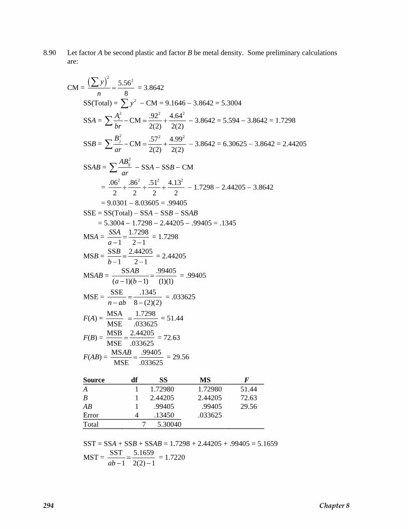
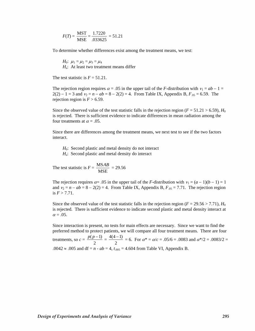
8.90 Let factor A be second plastic and factor B be metal density. Some preliminary calculations are:

CM = ( )2

25.568

yn

=∑ = 3.8642

SS(Total) = − CM = 9.1646 − 3.8642 = 5.3004 2y∑ SSA =

2 2 2.92 4.64CM2(2) 2(2)

iAbr

− = +∑ − 3.8642 = 5.594 − 3.8642 = 1.7298

SSB = 2 2 2.57 4.99CM

2(2) 2(2)jB

ar− = +∑ − 3.8642 = 6.30625 − 3.8642 = 2.44205

SSAB = 2ijAB

ar∑ − SSA − SSB − CM

= 2 2 2.06 .86 .51 4.13

2 2 2 2+ + +

2

− 1.7298 − 2.44205 − 3.8642

= 9.0301 − 8.03605 = .99405 SSE = SS(Total) − SSA − SSB − SSAB = 5.3004 − 1.7298 − 2.44205 − .99405 = .1345

MSA = 1.7298 1 2 1

SSAa

=− −

= 1.7298

MSB = SS 2.44205 1 2 1

Bb

=− −

= 2.44205

MSAB = SS .99405 ( 1)( 1) (1)(1)

ABa b

=− −

= .99405

MSE = SSE .1345 8 (2)(2)n ab

=− −

= .033625

F(A) = MSA 1.7298 MSE .033625

= = 51.44

F(B) = MSB 2.44205 MSE .033625

= = 72.63

F(AB) = MS .99405 MSE .033625

AB= = 29.56

Source df SS MS F A 1 1.72980 1.72980 51.44 B 1 2.44205 2.44205 72.63 AB 1 .99405 .99405 29.56 Error 4 .13450 .033625 Total 7 5.30040

SST = SSA + SSB + SSAB = 1.7298 + 2.44205 + .99405 = 5.1659

MST = SST 5.1659 1 2(2) 1ab

=− −

= 1.7220

294 Chapter 8

F(T) = MST 1.7220 = MSE .033625

= 51.21

To determine whether differences exist among the treatment means, we test: H0: μ1 = μ2 = μ3 = μ4

Ha: At least two treatment means differ The test statistic is F = 51.21. The rejection region requires α = .05 in the upper tail of the F-distribution with ν1 = ab − 1 =

2(2) − 1 = 3 and ν2 = n − ab = 8 − 2(2) = 4. From Table IX, Appendix B, F.05 = 6.59. The rejection region is F > 6.59.

Since the observed value of the test statistic falls in the rejection region (F = 51.21 > 6.59), H0

is rejected. There is sufficient evidence to indicate differences in mean radiation among the four treatments at α = .05.

Since there are differences among the treatment means, we next test to see if the two factors

interact. H0: Second plastic and metal density do not interact Ha: Second plastic and metal density do interact


AB = 29.56

The rejection requires α= .05 in the upper tail of the F-distribution with ν1 = (a − 1)(b − 1) = 1

and ν2 = n − ab = 8 − 2(2) = 4. From Table IX, Appendix B, F.05 = 7.71. The rejection region is F > 7.71.

Since the observed value of the test statistic falls in the rejection region (F = 29.56 > 7.71), H0

is rejected. There is sufficient evidence to indicate second plastic and metal density interact at α = .05.

Since interaction is present, no tests for main effects are necessary. Since we want to find the

preferred method to protect patients, we will compare all four treatment means. There are four

treatments, so c = ( 12

)p p − = 4(4 1)2

− = 6. For α* = α/c = .05/6 = .0083 and α*/2 = .0083/2 =

.0042 ≈ .005 and df = n - ab = 4, t.005 = 4.604 from Table VI, Appendix B.


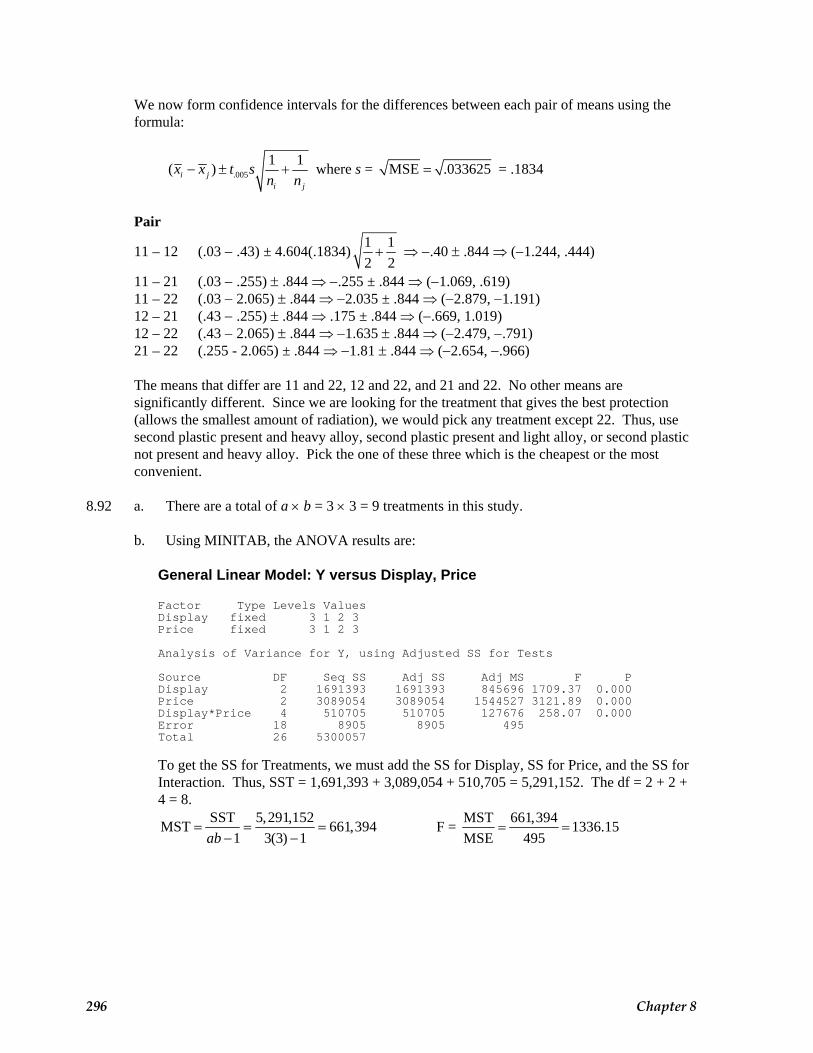
We now form confidence intervals for the differences between each pair of means using the formula:

.0051 1( )i j

i j

x x t sn n

− ± + where s = MSE .033625= = .1834

Pair

11 – 12 (.03 − .43) ± 4.604(.1834) 1 12 2+ ⇒ −.40 ± .844 ⇒ (−1.244, .444)

11 – 21 (.03 − .255) ± .844 ⇒ −.255 ± .844 ⇒ (−1.069, .619) 11 – 22 (.03 − 2.065) ± .844 ⇒ −2.035 ± .844 ⇒ (−2.879, −1.191) 12 – 21 (.43 − .255) ± .844 ⇒ .175 ± .844 ⇒ (−.669, 1.019) 12 – 22 (.43 − 2.065) ± .844 ⇒ −1.635 ± .844 ⇒ (−2.479, −.791) 21 – 22 (.255 - 2.065) ± .844 ⇒ −1.81 ± .844 ⇒ (−2.654, −.966) The means that differ are 11 and 22, 12 and 22, and 21 and 22. No other means are

significantly different. Since we are looking for the treatment that gives the best protection (allows the smallest amount of radiation), we would pick any treatment except 22. Thus, use second plastic present and heavy alloy, second plastic present and light alloy, or second plastic not present and heavy alloy. Pick the one of these three which is the cheapest or the most convenient.

8.92 a. There are a total of a × b = 3 × 3 = 9 treatments in this study.

b. Using MINITAB, the ANOVA results are:

General Linear Model: Y versus Display, Price

Factor Type Levels Values Display fixed 3 1 2 3 Price fixed 3 1 2 3

Analysis of Variance for Y, using Adjusted SS for Tests

Source DF Seq SS Adj SS Adj MS F P Display 2 1691393 1691393 845696 1709.37 0.000 Price 2 3089054 3089054 1544527 3121.89 0.000 Display*Price 4 510705 510705 127676 258.07 0.000 Error 18 8905 8905 495 Total 26 5300057

To get the SS for Treatments, we must add the SS for Display, SS for Price, and the SS for Interaction. Thus, SST = 1,691,393 + 3,089,054 + 510,705 = 5,291,152. The df = 2 + 2 + 4 = 8.

SST 5,291,152MST 661,3941 3(3) 1ab

= = =− −

MST 661,394F = 1336.15MSE 495

= =

296 Chapter 8

To determine whether the treatment means differ, we test: H0: μ1 = μ2 = ⋅⋅⋅ = μ9



= 1336.15

The rejection region requires α = .10 in the upper tail of the F-distribution with ν1 = ab − 1 = 3(3) − 1 = 8 and ν2 = n − ab = 27 − 3(3) = 18. From Table VIII, Appendix B,

F.10 = 2.04. The rejection region is F > 2.04. Since the observed value of the test statistic falls in the rejection region (F = 1336.15 >

2.04), H0 is rejected. There is sufficient evidence to indicate the treatment means differ at α = .10.

c. Since there are differences among the treatment means, we next test for the presence of

interaction. H0: Factors A and B do not interact to affect the response means Ha: Factors A and B do interact to affect the response means


AB = 258.07

The rejection region requires α = .10 in the upper tail of the F-distribution with ν1 = (a − 1)(b − 1) = (3 − 1)(3 − 1) = 4 and ν2 = n − ab = 17 − 3(3) = 18. From Table VIII,

Appendix B, F.10 = 2.29. The rejection region is F > 2.29. Since the observed value of the test statistic falls in the rejection region (F = 258.07 >

2.29), H0 is rejected. There is sufficient evidence to indicate the two factors interact at α = .10.

d. The main effect tests are not warranted since interaction is present in part c. e. The nine treatment means need to be compared. f. From the graph, if the like letters are connected, the lines are not parallel. This implies

interaction is present. This agrees with the results of part c.


8.94 a. This is a completely randomized design with a complete four-factor factorial design. b. There are a total of 2 × 2 × 2 × 2 = 16 treatments. c. Using SAS, the output is:

Analysis of Variance Procedure

Dependent Variable: Y

Sum of Mean

Source DF Squares Square F Value Pr > F

Model 15 546745.50 36449.70 5.11 0.0012

Error 16 114062.00 7128.88

Corrected Total 31 660807.50

R-Square C.V. Root MSE Y Mean

0.827390 41.46478 84.433 203.63

Source DF Anova SS Mean Square F Value Pr > F

SPEED 1 56784.50 56784.50 7.97 0.0123

FEED 1 21218.00 21218.00 2.98 0.1037

SPEED*FEED 1 55444.50 55444.50 7.78 0.0131

COLLET 1 165025.13 165025.13 23.15 0.0002

SPEED*COLLET 1 44253.13 44253.13 6.21 0.0241

FEED*COLLET 1 142311.13 142311.13 19.96 0.0004

SPEED*FEED*COLLET 1 54946.13 54946.13 7.71 0.0135

WEAR 1 378.13 378.13 0.05 0.8208

SPEED*WEAR 1 1540.13 1540.13 0.22 0.6483

FEED*WEAR 1 946.13 946.13 0.13 0.7204

SPEED*FEED*WEAR 1 528.13 528.13 0.07 0.7890

COLLET*WEAR 1 1682.00 1682.00 0.24 0.6337

SPEED*COLLET*WEAR 1 512.00 512.00 0.07 0.7921

FEED*COLLET*WEAR 1 72.00 72.00 0.01 0.9212

SPEE*FEED*COLLE*WEAR 1 1104.50 1104.50 0.15 0.6991

d. To determine if the interaction terms are significant, we must add together the sum of squares for all interaction terms as well as the degrees of freedom.

SS(Interaction) = 55,444.50 + 44,253.13 + 142,311.13 + 54,946.13 + 1,540.13 + 946.13 + 528.13 + 1,682.00 + 512.00 + 72.00 + 1,104.50 = 303,339.78 df(Interaction) = 11

MS(Interaction) = SS(Interacton)df(Interaction)

= 303,339.7811

= 27,576.34364

F(Interaction) = MS(Interaction)MSE

= 27,576.343647128.88

= 3.87

298 Chapter 8

To determine if interaction effects are present, we test: H0: No interaction effects exist Ha: Interaction effects exist The test statistic is F = 3.87. The rejection region requires α = .05 in the upper tail of the F-distribution with ν1 = 11

and ν2 = 16. From Table IX, Appendix B, F.05 ≈ 2.49. The rejection region is F > 2.49. Since the observed value of the test statistic falls in the rejection region (F = 3.87 > 2.49),

H0 is rejected. There is sufficient evidence to indicate that interaction effects exist at α = .05.

Since the sums of squares for a balanced factorial design are independent of each other,

we can look at the SAS output to determine which of the interaction effects are significant. The three-way interaction between speed, feed, and collet is significant

(p = .0135). There are three two-way interactions with p-values less than .05. However, all of these two-way interaction terms are imbedded in the significant three-way interaction term.

e. Yes. Since the significant interaction terms do not include wear, it would be necessary to

perform the main effect test for wear. All other main effects are contained in a significant interaction term.

To determine if the mean finish measurements differ for the different levels of wear, we

test: H0: The mean finish measurements for the two levels of wear are the same Ha: The mean finish measurements for the two levels of wear are different The test statistic is t = 0.05. The rejection region requires α = .05 in the upper tail of the F-distribution with ν1 = 1 and

ν2 = 16. From Table IX, Appendix B, F.05 = 4.49. The rejection region is F > 4.49. Since the observed value of the test statistic does not fall in the rejection region (F = .05

>/ 4.49), H0 is not rejected. There is insufficient evidence to indicate that the mean finish measurements differ for the different levels of wear at α = .05.

f. We must assume that: i. The populations sampled from are normal. ii. The population variances are the same. iii. The samples are random and independent.


Date post:	11-May-2018
Category:	Documents
Upload:	lycong
View:	233 times
Download:	1 times

Design of Experiments and Analysis of Variance...

Documents