76
DR. SHASHANK SHEKHAR MSE, IIT KANPUR FEB 19 TH 2016 TEQIP (IIT KANPUR) Design of Experiments
D R . S H A S H A N K S H E K H A R
M S E , I I T K A N P U R
F E B 1 9 T H 2 0 1 6
T E Q I P ( I I T K A N P U R )
Design of Experiments

Data Analysis
ShS (TEQIP Feb 19th-21st 2016)
2
Ask a Question
What to measure and
how
Chose method and collect data
Summarize data
Analyze data
Draw Conclusions
https://www.bcps.org/offices/lis/researchcourse/statistics_role.html
List of Topics
Objective of experiment
Strategy of Experimentation
Replication, Repetition and Randomization
Various approaches of experimentation
Guidelines for designing experiments
3
ShS (TEQIP Feb 19th-21st 2016)
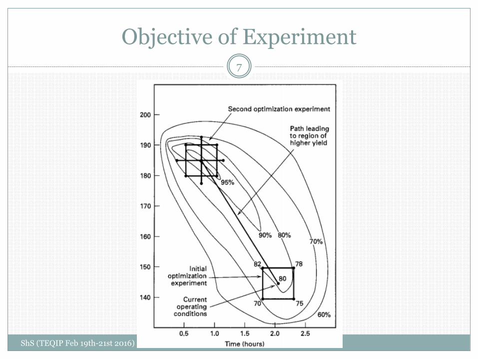
Objective of Experiment
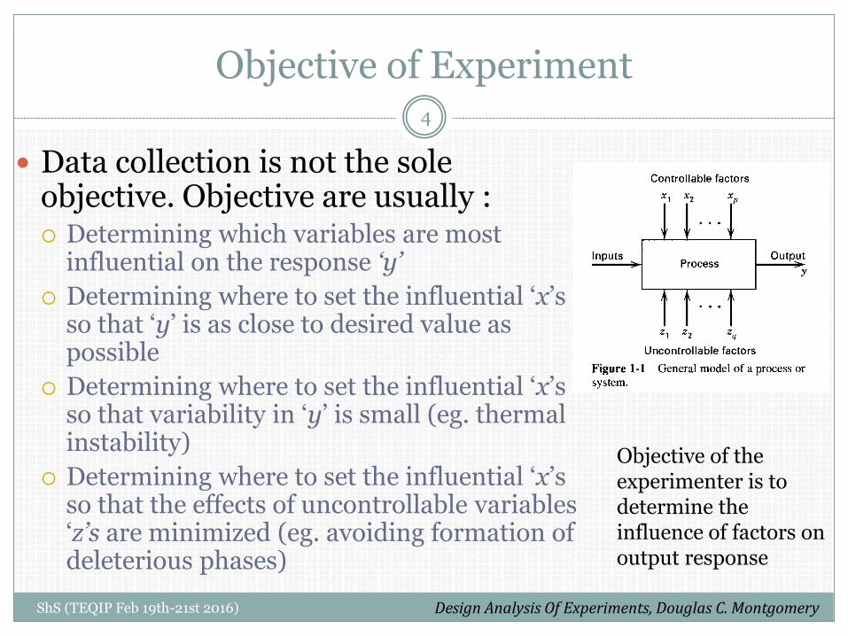
Data collection is not the sole objective. Objective are usually : Determining which variables are most
influential on the response ‘y’
Determining where to set the influential ‘x’s so that ‘y’ is as close to desired value as possible
Determining where to set the influential ‘x’s so that variability in ‘y’ is small (eg. thermal instability)
Determining where to set the influential ‘x’s so that the effects of uncontrollable variables ‘z’s are minimized (eg. avoiding formation of deleterious phases)
Objective of the experimenter is to determine the influence of factors on output response
4
ShS (TEQIP Feb 19th-21st 2016) Design Analysis Of Experiments, Douglas C. Montgomery

Strategy of Experimentation
Experiment may be defined as a test or a series of tests in which purposeful changes are made to the input variables of a process or system so that we may observe and identify the reasons for changes that may be observed in the output response
5
ShS (TEQIP Feb 19th-21st 2016)
An Example
A food processor may be interested in studying the effect of cooking medium (viz. with butter and with ghee) on quality of these cooked popcorns. His objective can be to determine which medium produces the best quality popcorn.
He may conduct tests on a number of collected samples in two different mediums and cook them and measure the quality to compare the effect of source. The quality may be determined, by say, the fraction of pop-corns that fracture under certain pressure. The average fraction of the properly cooked popcorns in the two mediums will be used to determine if there is a difference and which one produces better quality.
6
ShS (TEQIP Feb 19th-21st 2016)
Objective of Experiment
ShS (TEQIP Feb 19th-21st 2016)
7
Example: Questions to ponder
Are there any other factors that might affect quality that should be investigated (eg. Electrical Power of cooking system, time of cooking, moisture, room temperature, room humidity)
How many samples are required for each condition
In what order should the data be collected (eg. what if there is a drift in measurement values)
What method of data analysis should be used
What difference in average fraction between the two cooking media will be considered important (eg. ANOVA)
8
ShS (TEQIP Feb 19th-21st 2016)
Example: Data Collection
Method of data collection is also important
Suppose that the food scientist in the above experiment used specimens from one batch in the butter and specimens from a second batch in ghee
Engineer measures fractured fraction of all the samples cooked in one medium and then the fractured fractions cooked in the other medium
So what is the right method?
Completely randomized design is required
9
ShS (TEQIP Feb 19th-21st 2016)

Components of an Experiment
ShS (TEQIP Feb 19th-21st 2016)
10
A good experimental design must:
Avoid systematic error: it can lead to bias in comparison
Be precise: Random errors need to be reduced
Allow estimation of error: Permits statistical inference of confidence interval etc.
Have broad validity: sample should be good representation to be valid for the whole population
Basic Principles
ShS (TEQIP Feb 19th-21st 2016)
11
Randomization – Random allocation and order
Averaging out
Blocking – to improve precision in comparisons
Replication
Replication vs repeated measurements
Proper selection of sample (where should the corn samples be picked from)
Haphazard is not randomized
ShS (TEQIP Feb 19th-21st 2016)
12
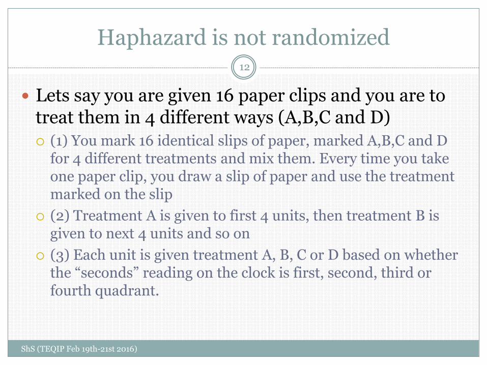
Lets say you are given 16 paper clips and you are to treat them in 4 different ways (A,B,C and D)
(1) You mark 16 identical slips of paper, marked A,B,C and D for 4 different treatments and mix them. Every time you take one paper clip, you draw a slip of paper and use the treatment marked on the slip
(2) Treatment A is given to first 4 units, then treatment B is given to next 4 units and so on
(3) Each unit is given treatment A, B, C or D based on whether the “seconds” reading on the clock is first, second, third or fourth quadrant.

Approaches
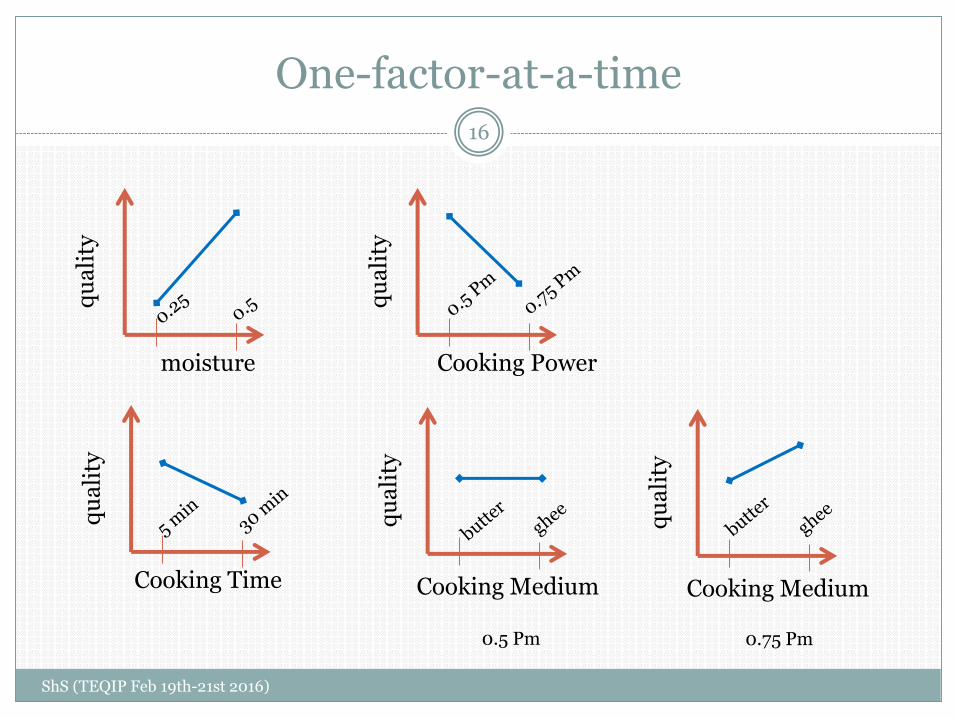
Lets say that there are four factors that need to be considered to understand the response. Lets says quality, (in terms of percentage cracked) is the response that you are interested in maximizing, and the factors are: time of cooking and (t=5mins or t = 30mins)
cooking medium (butter or ghee)
Power of equipment (P= 0.5Pm or P = 0.75 Pm)
Moisture fraction (strain = 0.25 or strain = 0.5)
How will you sort through each and every factor and its effect on quality? For simplicity only two states of each factor are taken and it is given that you have only 8 samples.
13
ShS (TEQIP Feb 19th-21st 2016)
Approaches
Best-guess approach: Test for arbitrary combination and see the outcome. During the test however you noticed that all high power conditions conditions resulted in lower quality and so you may decide to use lower power and keep other factors same as earlier. This process can go on until all the factors are optimized
Disadvantages One has to keep trying combinations, without any guarantee of
success
If the initial combination produces acceptable result, one may be tempted to stop testing
14
ShS (TEQIP Feb 19th-21st 2016)
Approaches
One-factor-at-a-time: Select a baseline set of levels, for each factor, then successively vary each factor over its range with other factors held constant at the baseline level. A series of graphs can represent the output as a response to the change in these factors Interpretation is simple and straight forward, however
interaction between the factors is not highlighted (An interaction is the failure of the one factor to produce the same effect on the response at different levels of another factor)
One-factor-at-a-time experiments are always less efficient that the other methods based on a statistical approach to design
15
ShS (TEQIP Feb 19th-21st 2016)
One-factor-at-a-time
ShS (TEQIP Feb 19th-21st 2016)
16
qu
ali
ty
Cooking Medium
qu
ali
ty
moistureq
ua
lity
Cooking Power
qu
ali
ty
Cooking Time
qu
ali
ty
Cooking Medium
0.5 Pm 0.75 Pm
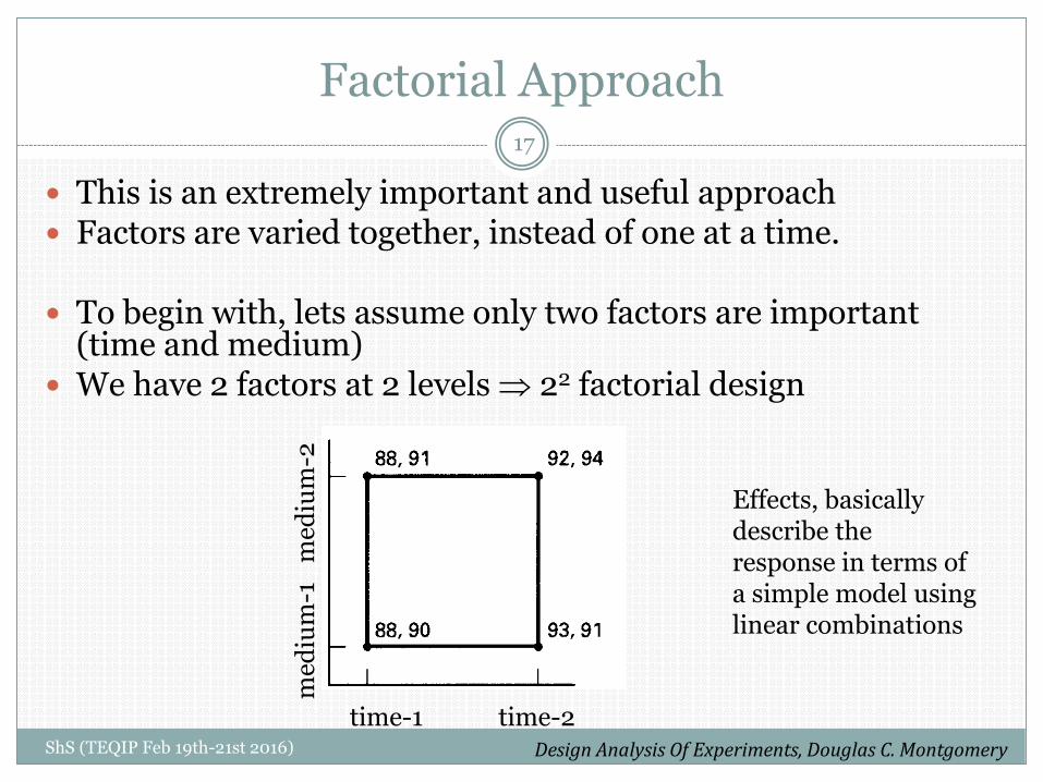
Factorial Approach
This is an extremely important and useful approach Factors are varied together, instead of one at a time.
To begin with, lets assume only two factors are important (time and medium)
We have 2 factors at 2 levels 22 factorial design
time-1 time-2
med
ium
-1
med
ium
-2
Effects, basically describe the response in terms of a simple model using linear combinations
17
ShS (TEQIP Feb 19th-21st 2016) Design Analysis Of Experiments, Douglas C. Montgomery

Factorial Approach
ShS (TEQIP Feb 19th-21st 2016)
18
time-1 time-2
med
ium
-1
med
ium
-2
A= Effect of time = (92+94+93+91)/4 – (88+91+88+90)/4 = 3.25
B = Effect of medium =(88+91+92+94)/4 – (88+90+93+91)/4 =0.75
AB = Measure of interaction =(92+94+88+90)/4 – (88+91+93+91)/4 =0.25
Average = 90.875
A fitted regression model to express the response in terms of the two parameters:
y= 90.875 + A/2*x1 + B/2*x2 +AB/2* x1x2y = 90.875 + 1.625x1 + 0.375x2 + 0.125x1x2
Statistical testing is required to determine whether any of these effects differ from zero
Design Analysis Of Experiments, Douglas C. Montgomery
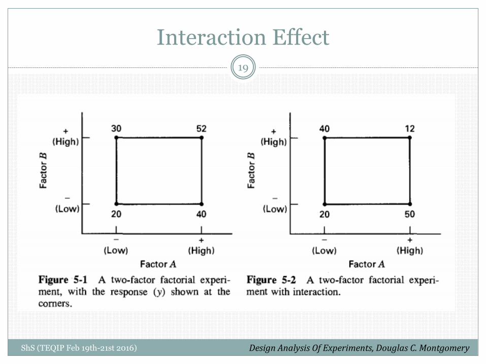
Interaction Effect
ShS (TEQIP Feb 19th-21st 2016)
19
Design Analysis Of Experiments, Douglas C. Montgomery
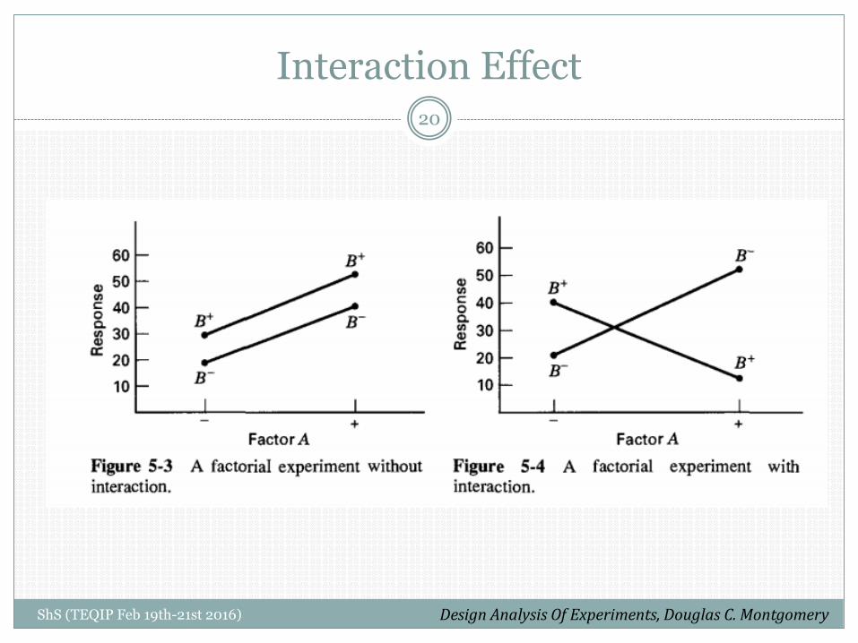
Interaction Effect
ShS (TEQIP Feb 19th-21st 2016)
20
Design Analysis Of Experiments, Douglas C. Montgomery
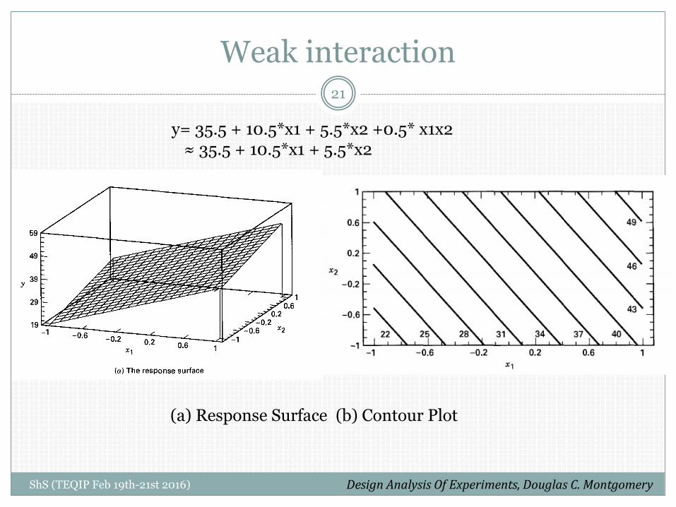
Weak interaction21
ShS (TEQIP Feb 19th-21st 2016)
y= 35.5 + 10.5*x1 + 5.5*x2 +0.5* x1x2≈ 35.5 + 10.5*x1 + 5.5*x2
Design Analysis Of Experiments, Douglas C. Montgomery
(a) Response Surface (b) Contour Plot
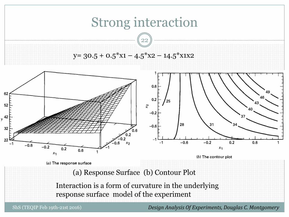
Strong interaction
ShS (TEQIP Feb 19th-21st 2016)
22
y= 30.5 + 0.5*x1 – 4.5*x2 – 14.5*x1x2
Interaction is a form of curvature in the underlying response surface model of the experiment
Design Analysis Of Experiments, Douglas C. Montgomery
(a) Response Surface (b) Contour Plot
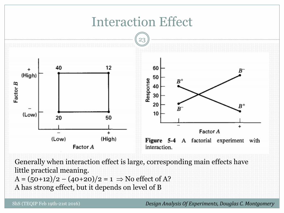
Interaction Effect
ShS (TEQIP Feb 19th-21st 2016)
23
Generally when interaction effect is large, corresponding main effects have little practical meaning. A = (50+12)/2 – (40+20)/2 = 1 No effect of A?A has strong effect, but it depends on level of B
Design Analysis Of Experiments, Douglas C. Montgomery

Advantages of Factorial
ShS (TEQIP Feb 19th-21st 2016)
24
Lets again look at two factors with two levels
No. of experiments for one-factor-approach =
No. of experiments for factorial approach =
Efficiency of factorial approach =
If A-B+ and A+B- gave a better response, then what about A+B+?
Design Analysis Of Experiments, Douglas C. Montgomery
6
4
6/4 = 1.5
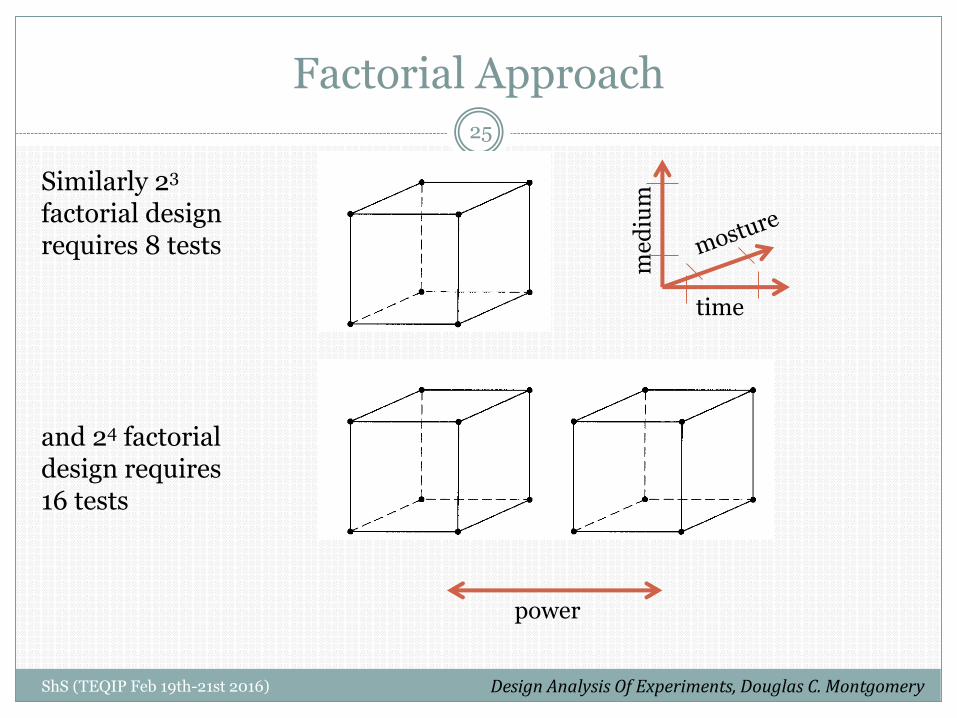
Factorial Approach
Similarly 23
factorial design requires 8 tests
and 24 factorial design requires 16 tests
power
time
med
ium
25
ShS (TEQIP Feb 19th-21st 2016) Design Analysis Of Experiments, Douglas C. Montgomery
Factorial Approach
If there are k factors, each at two levels, the factorial design would require 2k tests
4 factors with 2 levels require 16 tests
10 factors with 2 levels require 1024 tests!!
This is clearly infeasible from time and resource point of view
Fractional factorial design can be used
26
ShS (TEQIP Feb 19th-21st 2016)
Fractional Factorial Design
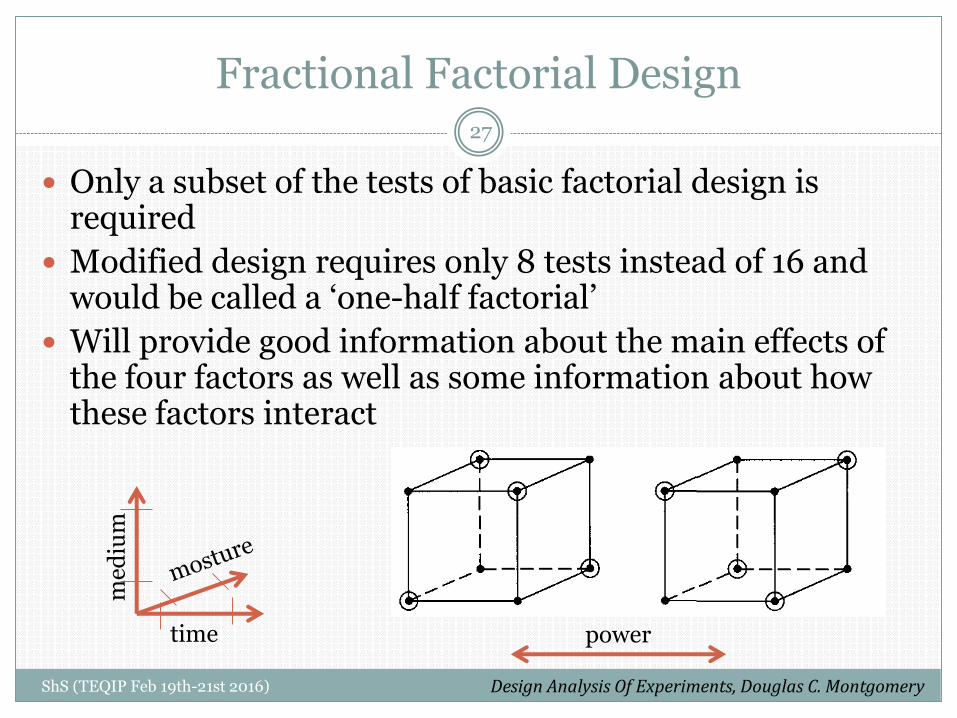
Only a subset of the tests of basic factorial design is required
Modified design requires only 8 tests instead of 16 and would be called a ‘one-half factorial’
Will provide good information about the main effects of the four factors as well as some information about how these factors interact
power
27
ShS (TEQIP Feb 19th-21st 2016) Design Analysis Of Experiments, Douglas C. Montgomery
time
med
ium
Fractional Factorial Designs
If reasonable assumptions can be made that certain high-order interactions are negligible, then fractional factorial designs prove to be very effective
A major use of fractional factorial is in “screening experiments” (eg to identify those factors that have large effects)
It is based on the principle that when there are several variables, the system or process is likely to be driven primarily by some of the main effects and low-order interactions
It is possible to combine the runs of two or more fractional factorial to assemble sequentially a larger design to estimate the factor effects and interactions of interests
28
ShS (TEQIP Feb 19th-21st 2016)
Fractional Factorial Approach
ShS (TEQIP Feb 19th-21st 2016)
29
Design Analysis Of Experiments, Douglas C. Montgomery
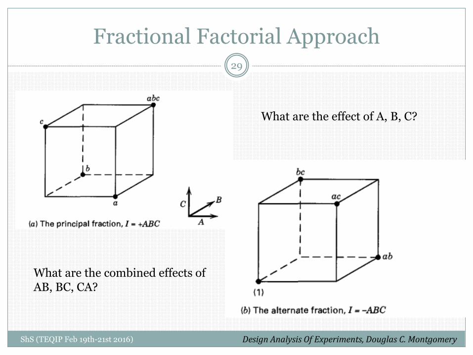
What are the effect of A, B, C?
What are the combined effects of AB, BC, CA?
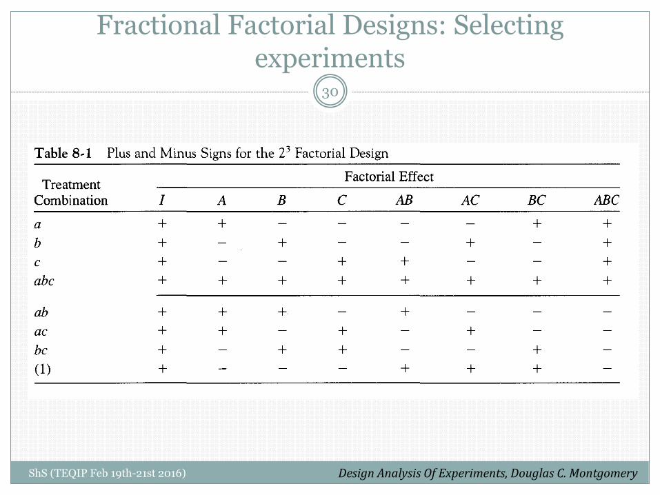
Fractional Factorial Designs: Selecting experiments
30
ShS (TEQIP Feb 19th-21st 2016) Design Analysis Of Experiments, Douglas C. Montgomery
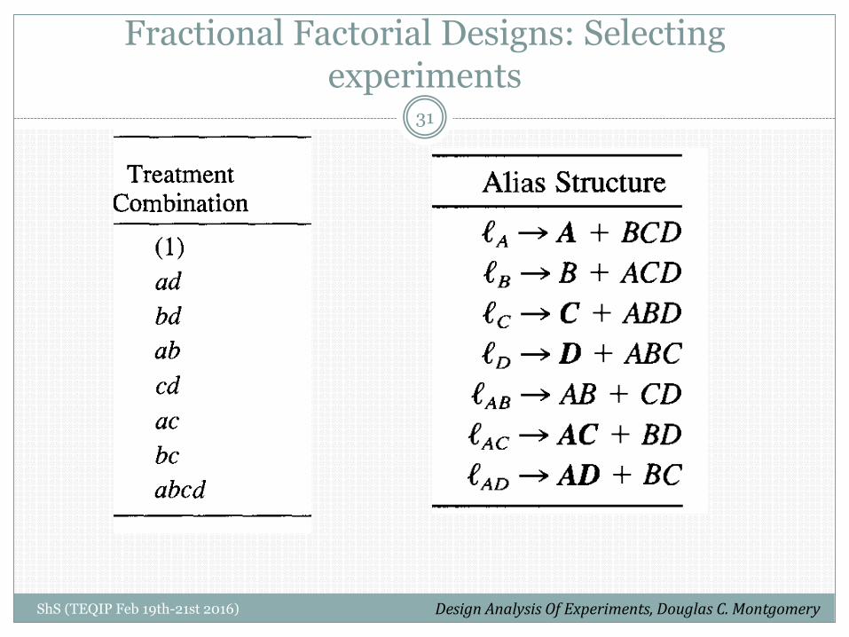
Fractional Factorial Designs: Selecting experiments
31
ShS (TEQIP Feb 19th-21st 2016) Design Analysis Of Experiments, Douglas C. Montgomery

Guidelines for Designing Experiments
Recognition of and statement of the problem (eg. is the objective to characterize response or is it understood well enough to be optimized. Or, is the objective to confirm a discovery, stability)
Choice of factors, levels, and range (eg. are there fixed no. of levels or if there is a range, how many levels to select and how to select so as to represent the whole range)
Selection of the response variable (eg. Measurement of hardness is a better variable but not easy to measure on each popcorn; On the other hand fraction of fractured popcorn is easy to measure, but not a good representation)
32
ShS (TEQIP Feb 19th-21st 2016)
Guidelines for Designing Experiments
Choice of experimental design (eg. consideration of sample size, selection of suitable order for experiments, selecting the methodology based on the objectives)
Performing the experiment (be aware of uncontrollable parameters, sources of errors and other factors that might have been missed earlier. Egdrift in the values of the equipment being used)
Statistical analysis of the data (what does the data mean. How statistically significant or insignificant is a particular factor)
33
ShS (TEQIP Feb 19th-21st 2016)

D R . S H A S H A N K S H E K H A R
M S E , I I T K A N P U R
F E B 1 9 T H 2 0 1 6
T E Q I P ( I I T K A N P U R )
Data Presentation
Data Analysis
ShS (TEQIP Feb 19th-21st 2016)
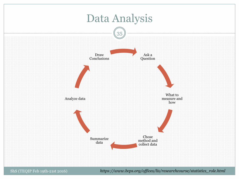
35
Ask a Question
What to measure and
how
Chose method and collect data
Summarize data
Analyze data
Draw Conclusions
https://www.bcps.org/offices/lis/researchcourse/statistics_role.html

List of Topics
Graphical and other means of presenting data
Graphical Summary
Plots
Histograms
Numerical Summary (Mean, Median, Mode etc)
Measures of spread of data
Variance and Standard deviation
Quantifying spread
Chebyshev’s Inequality
Standard Deviation versus Standard Error
36
ShS (TEQIP Feb 19th-21st 2016)

Accuracy vs Precision
Source: https://sites.google.com/a/apaches.k12.in.us/mr-evans-science-website/accuracy-vs-precision
37
ShS (TEQIP Feb 19th-21st 2016)
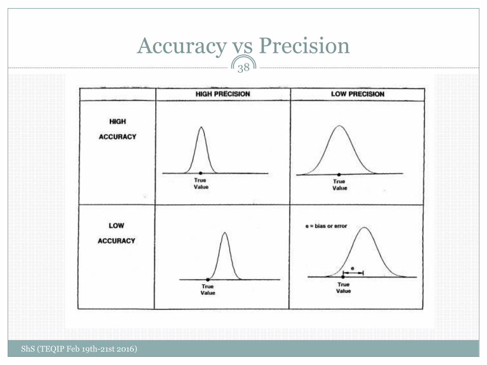
Accuracy vs Precision38
ShS (TEQIP Feb 19th-21st 2016)
Statistics
ShS (TEQIP Feb 19th-21st 2016)
39
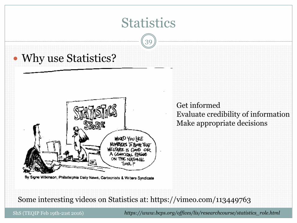
Why use Statistics?
https://www.bcps.org/offices/lis/researchcourse/statistics_role.html
Some interesting videos on Statistics at: https://vimeo.com/113449763
Get informedEvaluate credibility of informationMake appropriate decisions
Statistics
Why use Statistics?
Data Set: A collection of observations
Population vs Sample
Variable: A characteristic of the object
Univariate (height) versus Multivariate (height, weight, race…)
Numerical
Discreet (No. of employees; No. of grains)
Continuous (weight of boxer; Length or area of twin boundary)
Categorical
Ordinal (1st class, 2nd class, 3rd class railway coaches; Course No. MSE201, MSE301 etc)
Not-ordinal (Process condition-1, Process condition-2)
40
ShS (TEQIP Feb 19th-21st 2016)

Summarizing data
Comprehension in exchange of losing data
Graphical Summary
Categorical variable bar charts, pie charts
How not to construct charts
Numerical variables Guidelines to making plots
Numerical Summary
Mean (population versus sample)
Median
Mode
Point estimate of
41
ShS (TEQIP Feb 19th-21st 2016)
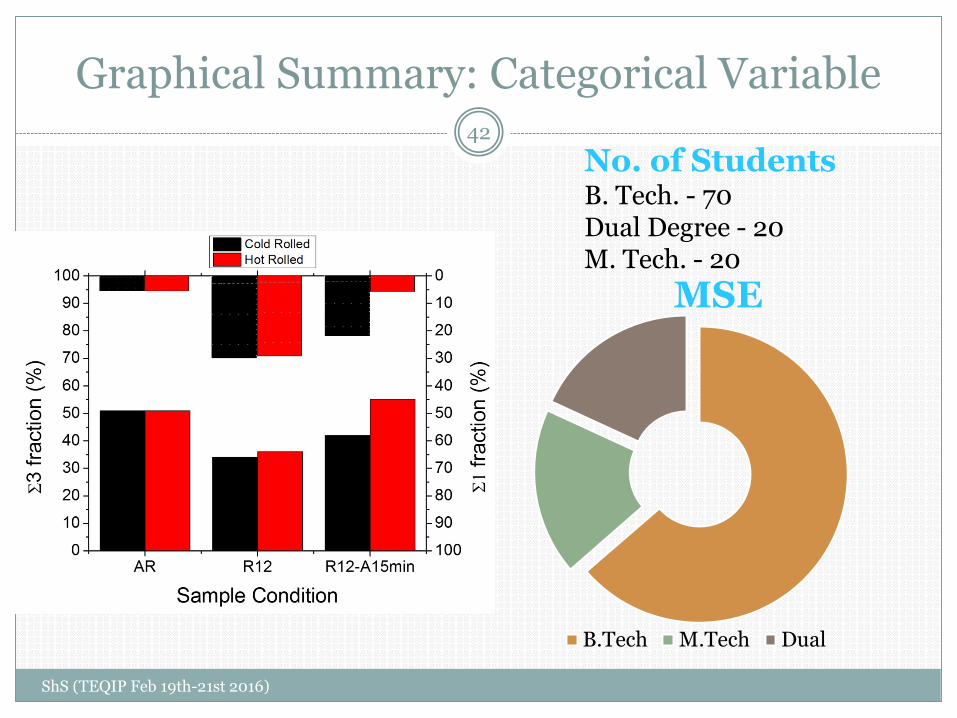
Graphical Summary: Categorical Variable
ShS (TEQIP Feb 19th-21st 2016)
42
MSE
B.Tech M.Tech Dual
No. of StudentsB. Tech. - 70Dual Degree - 20M. Tech. - 20
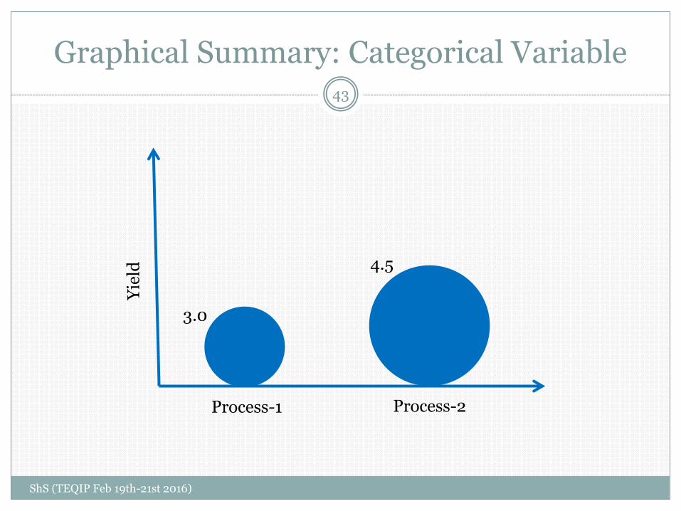
Graphical Summary: Categorical Variable
ShS (TEQIP Feb 19th-21st 2016)
43
Yie
ld
Process-1 Process-2
3.0
4.5
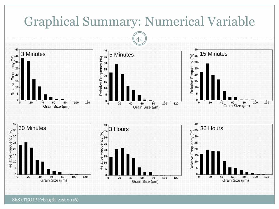
Graphical Summary: Numerical Variable
ShS (TEQIP Feb 19th-21st 2016)
44
0 20 40 60 80 100 1200
5
10
15
20
25
30
35
40
Re
lative F
req
ue
ncy (
%)
30 Minutes
Grain Size (m)
0 20 40 60 80 100 1200
5
10
15
20
25
30
35
40
5 Minutes
Grain Size (m)
Re
lative F
req
ue
ncy (
%)
0 20 40 60 80 100 1200
5
10
15
20
25
30
35
40
Re
lative F
req
ue
ncy (
%)
Grain Size (m)
3 Minutes
0 20 40 60 80 100 1200
5
10
15
20
25
30
35
40
36 Hours
Re
lative F
req
ue
ncy (
%)
Grain Size (m)
0 20 40 60 80 100 1200
5
10
15
20
25
30
35
40
Grain Size (m)
Re
lative F
req
ue
ncy (
%) 15 Minutes
0 20 40 60 80 100 1200
5
10
15
20
25
30
35
40
Grain Size (m)
3 Hours
Re
lative F
req
ue
ncy (
%)
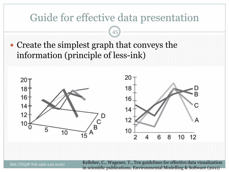
Guide for effective data presentation
ShS (TEQIP Feb 19th-21st 2016)
45
Create the simplest graph that conveys the information (principle of less-ink)
Kelleher, C., Wagener, T., Ten guidelines for effective data visualization in scientific publications, Environmental Modelling & Software (2011)
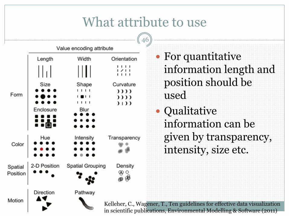
What attribute to use
ShS (TEQIP Feb 19th-21st 2016)
46
For quantitative information length and position should be used
Qualitative information can be given by transparency, intensity, size etc.
Kelleher, C., Wagener, T., Ten guidelines for effective data visualization in scientific publications, Environmental Modelling & Software (2011)
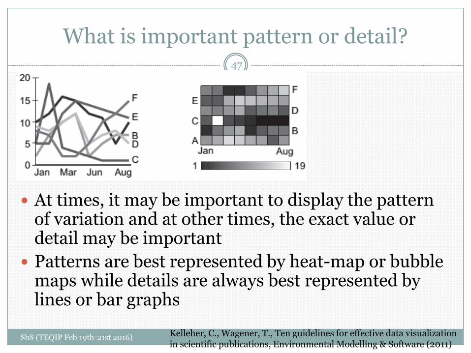
What is important pattern or detail?
ShS (TEQIP Feb 19th-21st 2016)
47
At times, it may be important to display the pattern of variation and at other times, the exact value or detail may be important
Patterns are best represented by heat-map or bubble maps while details are always best represented by lines or bar graphs
Kelleher, C., Wagener, T., Ten guidelines for effective data visualization in scientific publications, Environmental Modelling & Software (2011)
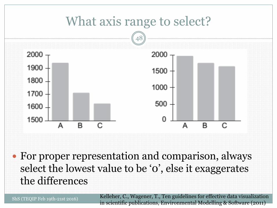
What axis range to select?
ShS (TEQIP Feb 19th-21st 2016)
48
For proper representation and comparison, always select the lowest value to be ‘0’, else it exaggerates the differences
Kelleher, C., Wagener, T., Ten guidelines for effective data visualization in scientific publications, Environmental Modelling & Software (2011)

How to represent scatter plot properly
ShS (TEQIP Feb 19th-21st 2016)
49
Scatter plot may also represent density of data points, hence utilizing transparency attribute may be useful
Kelleher, C., Wagener, T., Ten guidelines for effective data visualization in scientific publications, Environmental Modelling & Software (2011)
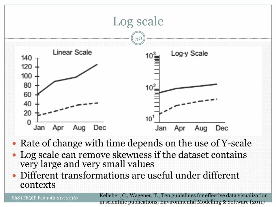
Log scale
ShS (TEQIP Feb 19th-21st 2016)
50
Rate of change with time depends on the use of Y-scale Log scale can remove skewness if the dataset contains
very large and very small values Different transformations are useful under different
contextsKelleher, C., Wagener, T., Ten guidelines for effective data visualization in scientific publications, Environmental Modelling & Software (2011)
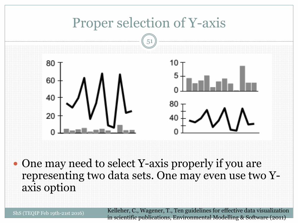
Proper selection of Y-axis
ShS (TEQIP Feb 19th-21st 2016)
51
One may need to select Y-axis properly if you are representing two data sets. One may even use two Y-axis option
Kelleher, C., Wagener, T., Ten guidelines for effective data visualization in scientific publications, Environmental Modelling & Software (2011)

Proper selection of color scheme
ShS (TEQIP Feb 19th-21st 2016)
52
Heat map may be represented in various color scheme
Selection depends on whether you want to emphasize intensity or diversion
Kelleher, C., Wagener, T., Ten guidelines for effective data visualization in scientific publications, Environmental Modelling & Software (2011)
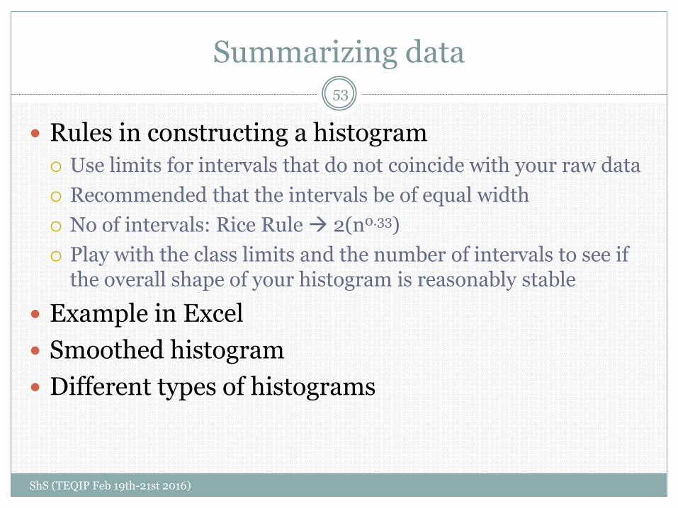
Summarizing data
Rules in constructing a histogram
Use limits for intervals that do not coincide with your raw data
Recommended that the intervals be of equal width
No of intervals: Rice Rule 2(n0.33)
Play with the class limits and the number of intervals to see if the overall shape of your histogram is reasonably stable
Example in Excel
Smoothed histogram
Different types of histograms
53
ShS (TEQIP Feb 19th-21st 2016)
Solved Example in Excel
ShS (TEQIP Feb 19th-21st 2016)
54
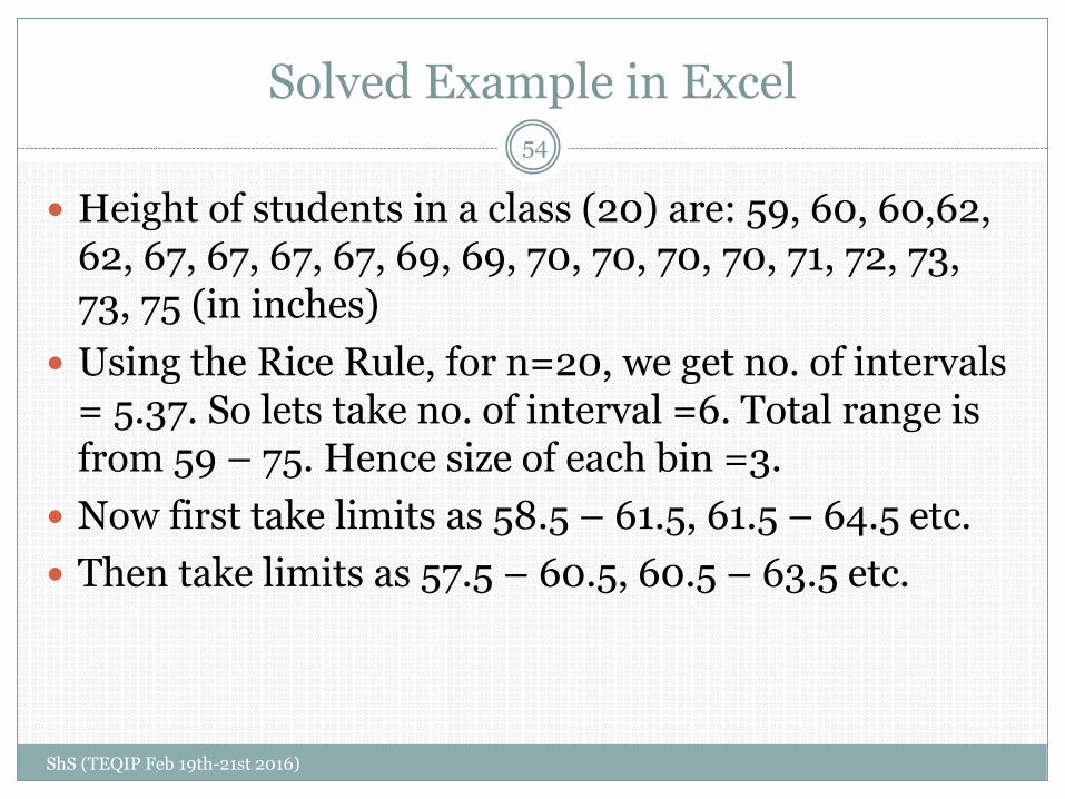
Height of students in a class (20) are: 59, 60, 60,62, 62, 67, 67, 67, 67, 69, 69, 70, 70, 70, 70, 71, 72, 73, 73, 75 (in inches)
Using the Rice Rule, for n=20, we get no. of intervals = 5.37. So lets take no. of interval =6. Total range is from 59 – 75. Hence size of each bin =3.
Now first take limits as 58.5 – 61.5, 61.5 – 64.5 etc.
Then take limits as 57.5 – 60.5, 60.5 – 63.5 etc.
Solved Example in Excel
ShS (TEQIP Feb 19th-21st 2016)
55
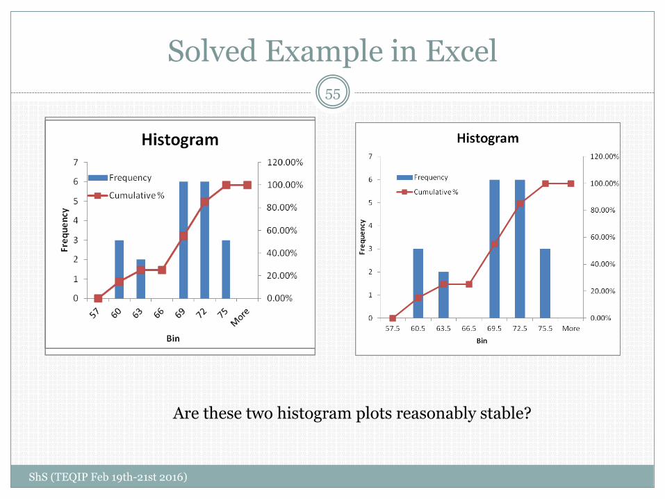
Are these two histogram plots reasonably stable?

Smoothed Histogram
ShS (TEQIP Feb 19th-21st 2016)
56
Smoothed histogram or density estimate can be obtained by taking center point of each limit and connecting a curve through the top of these histograms
Numerical Summary
ShS (TEQIP Feb 19th-21st 2016)
57
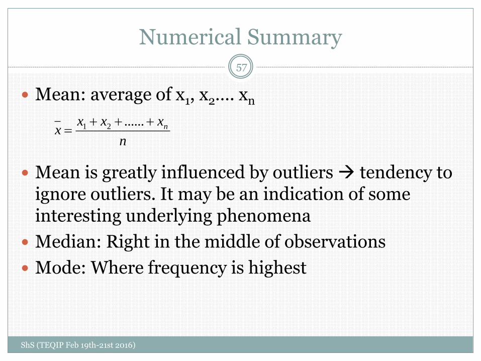
Mean: average of x1, x2…. xn
Mean is greatly influenced by outliers tendency to ignore outliers. It may be an indication of some interesting underlying phenomena
Median: Right in the middle of observations
Mode: Where frequency is highest
n
xxxx n
......21
Example
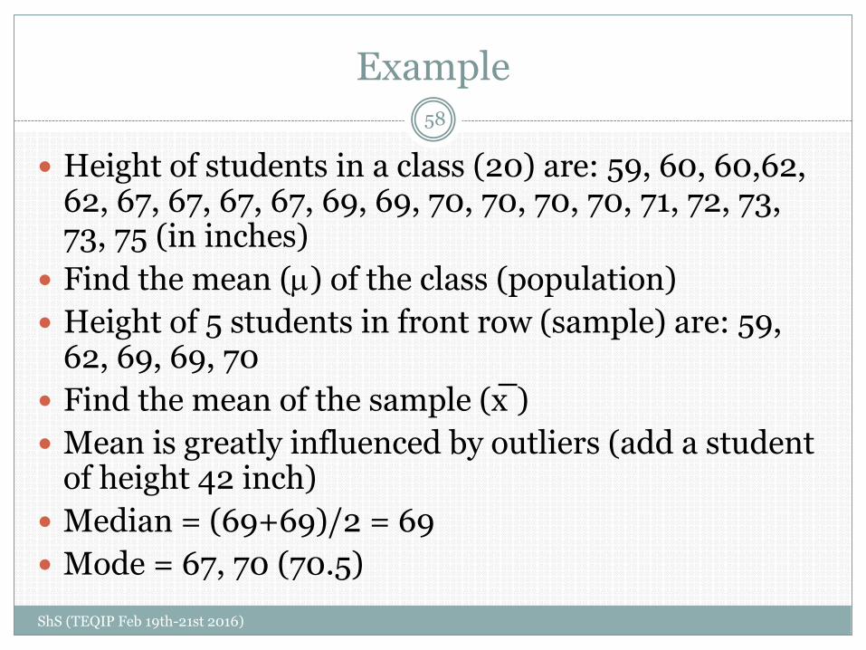
Height of students in a class (20) are: 59, 60, 60,62, 62, 67, 67, 67, 67, 69, 69, 70, 70, 70, 70, 71, 72, 73, 73, 75 (in inches)
Find the mean () of the class (population)
Height of 5 students in front row (sample) are: 59, 62, 69, 69, 70
Find the mean of the sample (x ̅ )
Mean is greatly influenced by outliers (add a student of height 42 inch)
Median = (69+69)/2 = 69
Mode = 67, 70 (70.5)
58
ShS (TEQIP Feb 19th-21st 2016)

Measures of spread
Different data set with same mean and median
Dataset A: -2, -1, 0, 1, 2
Dataset B: -10, -5, 0, 5, 10
Inter-quartile range (Q3-Q1)
Range (max-min)
Standard deviation and variance (s.d. = √variance)
Population vs Sample standard deviation
59
ShS (TEQIP Feb 19th-21st 2016)
1
)( 2
2
n
xxs
i
n
xi
2
2)(
x ̅ (A)=0; s(A)=1.55x ̅ (B)=0; s(B)=7.9
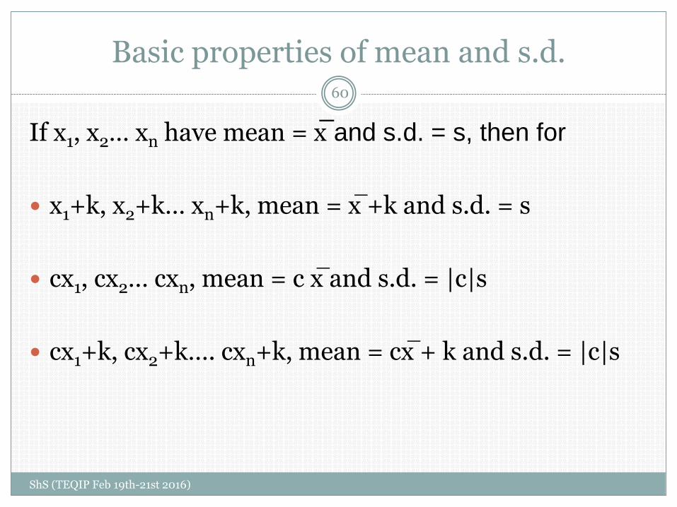
Basic properties of mean and s.d.
If x1, x2… xn have mean = x ̅ and s.d. = s, then for
x1+k, x2+k… xn+k, mean = x ̅ +k and s.d. = s
cx1, cx2… cxn, mean = c x ̅ and s.d. = |c|s
cx1+k, cx2+k…. cxn+k, mean = cx ̅ + k and s.d. = |c|s
60
ShS (TEQIP Feb 19th-21st 2016)
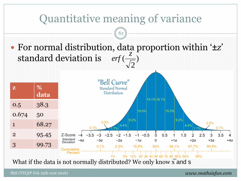
Quantitative meaning of variance
For normal distribution, data proportion within ‘±z’ standard deviation is )
2(
zerf
z % data
0.5 38.3
0.674 50
1 68.27
2 95.45
3 99.73
61
ShS (TEQIP Feb 19th-21st 2016)
What if the data is not normally distributed? We only know x ̅ and s
www.mathsisfun.com
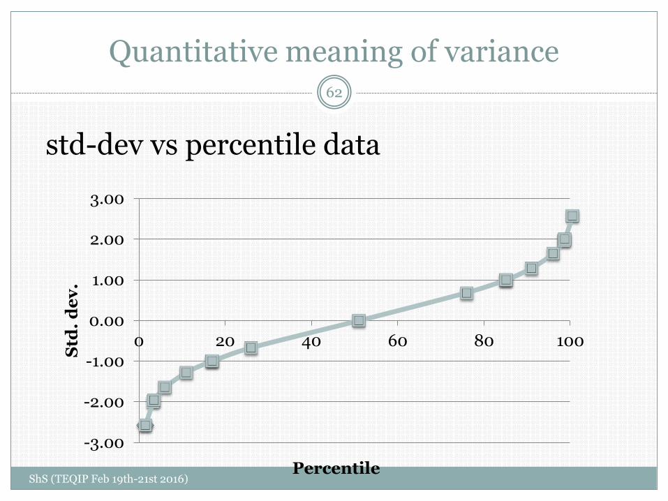
Quantitative meaning of variance
-3.00
-2.00
-1.00
0.00
1.00
2.00
3.00
0 20 40 60 80 100
Std
. d
ev
.
std-dev vs percentile data
62
ShS (TEQIP Feb 19th-21st 2016)Percentile
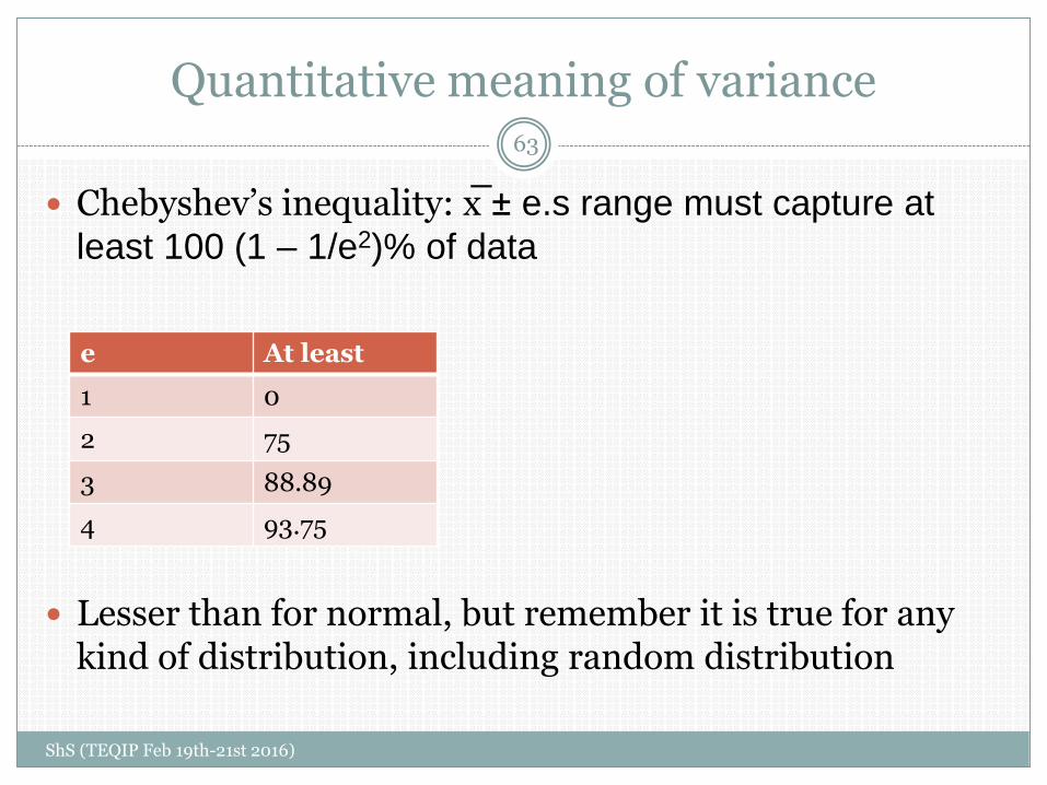
Quantitative meaning of variance
Chebyshev’s inequality: x̅ ± e.s range must capture at
least 100 (1 – 1/e2)% of data
Lesser than for normal, but remember it is true for any kind of distribution, including random distribution
e At least
1 0
2 75
3 88.89
4 93.75
63
ShS (TEQIP Feb 19th-21st 2016)

Example-2
ShS (TEQIP Feb 19th-21st 2016)
64
Example: Average of a midterm in a class of 55 students is 65 and s.d. =10. Cut-off for A is 85. What can you say about how many students got “A”
x ̅ = 65; s = 10; cut-off for A = 85
How many std. deviations away?
x ̅ ± e.10 = 85 e=2 at least 75% data within 65
± 20 (45-85)
% students getting more than 85% is less than 25%
of class (0.25*55 = 13.75)
Max no. of students getting ‘A’ = 13
Standard Error
ShS (TEQIP Feb 19th-21st 2016)
65
Standard error is the standard deviation of the sampling distribution of mean
Different samples drawn from the same population would in general have different values of the sample mean, although there will be a true mean (for a Gaussian distribution)
Std dev versus Std error
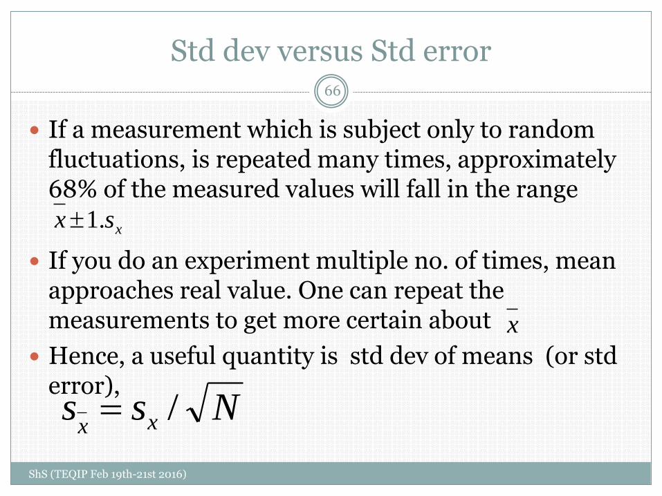
If a measurement which is subject only to random fluctuations, is repeated many times, approximately 68% of the measured values will fall in the range
If you do an experiment multiple no. of times, mean approaches real value. One can repeat the measurements to get more certain about
Hence, a useful quantity is std dev of means (or std error),
xsx .1
x
Nss xx/
66
ShS (TEQIP Feb 19th-21st 2016)

Example-4
Find, mean, s.d. and s.e. for the given data sets
Plot using error bars
67
ShS (TEQIP Feb 19th-21st 2016)
Class Experiment Analysis
ShS (TEQIP Feb 19th-21st 2016)
68
Lets first use data for uncoated sample
Calculate average for each group
Calculate average and std. dev. of raw data
Calculate average and std. dev of mean of each group
What should be the relation between std. dev of raw data and std dev of means?
What can you comment on this
Class Experiment Analysis
ShS (TEQIP Feb 19th-21st 2016)
69
Plot histograms for raw data and for means
What do you see?
Lets look closer at the raw data
One of the data point seems outlier
Plot after removing this. Looks good?
But, can we remove this data point?
Average = 7.4; Std. dev.= 4.8
Outlier = 24; How many std. dev away
Can we reject it?
3.45
3.875
Class Experiment Analysis
ShS (TEQIP Feb 19th-21st 2016)
70
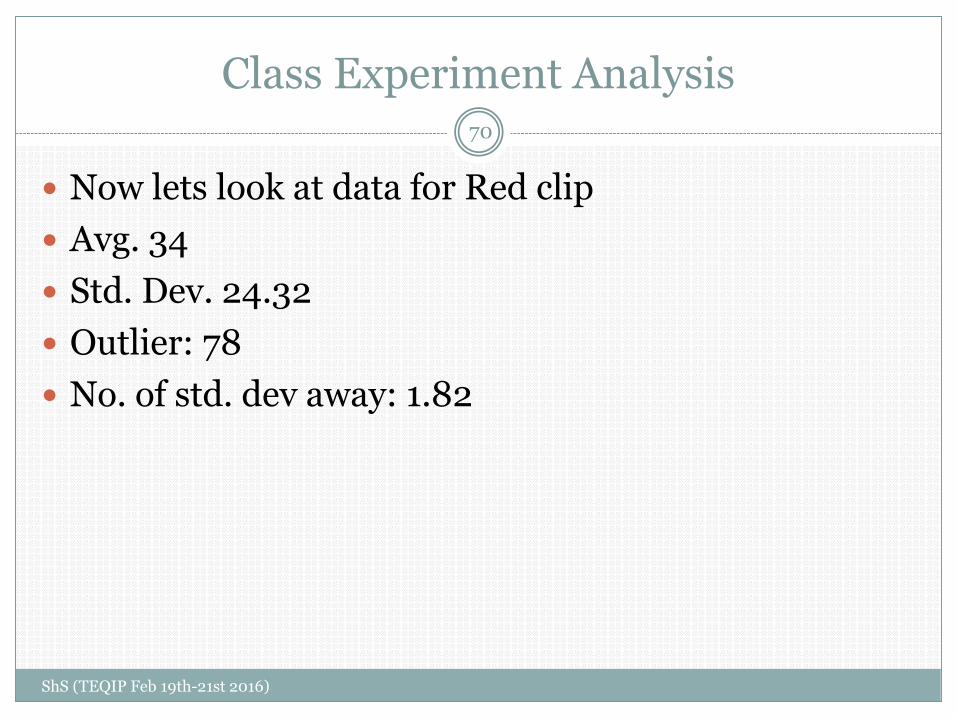
Now lets look at data for Red clip
Avg. 34
Std. Dev. 24.32
Outlier: 78
No. of std. dev away: 1.82

Example-4: Plotting Error bars
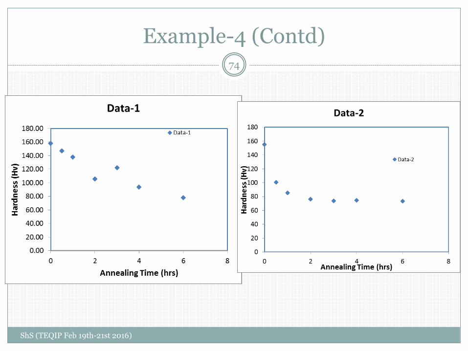
Time (hrs) hardness-1 error-1 hardness-2 error-2
0 158.0 3.5 155.0 5.3
0.5 146.9 3.2 100.6 10.3
1 137.7 7.3 85.4 3.8
2 105.9 19.6 76.4 2.6
3 122.3 17.0 75.5 -
4 93.7 15.1 74.5 4.1
6 78.2 2.0 73.5 3.1
71
ShS (TEQIP Feb 19th-21st 2016)
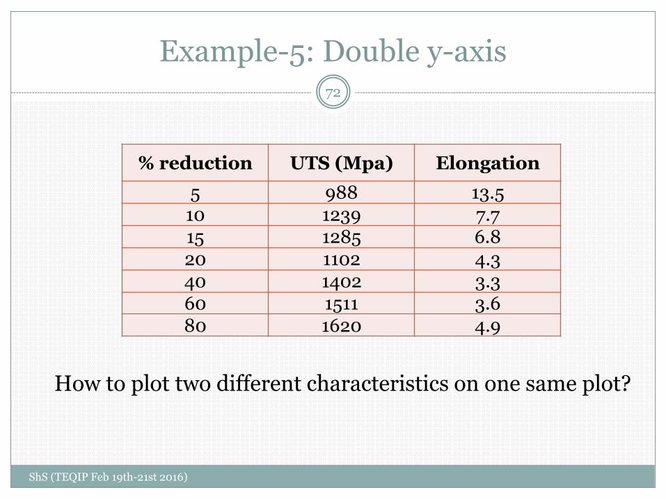
Example-5: Double y-axis
% reduction UTS (Mpa) Elongation
5 988 13.510 1239 7.715 1285 6.820 1102 4.340 1402 3.360 1511 3.680 1620 4.9
How to plot two different characteristics on one same plot?
72
ShS (TEQIP Feb 19th-21st 2016)

Example-5
ShS (TEQIP Feb 19th-21st 2016)
73
Example-4 (Contd)
ShS (TEQIP Feb 19th-21st 2016)
74
Summary
ShS (TEQIP Feb 19th-21st 2016)
75
Data presentation may look like a mundane task, but it involves a lot of intricacies
The sole objective of data presentation should be to convey the full picture to the viewer without hiding any information
Effective data presentation ensures that maximum information is conveyed in minimum ‘ink’

ShS (TEQIP Feb 19th-21st 2016) 76
Questions


