Page 1
HELSINKI UNIVERSITY OF TECHNOLOGY
Faculty of Electronics, Communications and Automation
Department of Radio Science and Engineering
Aki Karttunen
Design of feed systems for hologram-based compact antenna test ranges
The thesis was submitted in partial fulfilment for the degree of Licentiate of Science in
Technology in Espoo,
Supervisor
Professor Antti Räisänen
Second examiner
Pasi Ylä-Oijala, Ph.D.
Page 2
2
Helsinki University of Technology Abstract of the Licentiate’s Thesis
Author: Aki Karttunen
Name of the Thesis: Design of feed systems for hologram-based compact
antenna test ranges
Date: August 26, 2009 Number of pages:
106
Faculty: Faculty of Electronics, Communications and Automation
Professorship: Radio Engineering
Supervisor: Professor Antti Räisänen
Second examiner: Pasi Ylä-Oijala, Ph.D.
A designing method for feed systems for hologram-based compact antenna test ranges
(CATR) is developed. A hologram-based CATR can be used to test large antennas at
millimetre and submillimetre wavelengths. Feed systems are used to provide a modified
illumination for the hologram. Using the modified illumination from a feed system,
narrow slots can be avoided in the hologram pattern. Narrow slots are difficult to
manufacture accurately and limit the polarisation properties of the hologram.
Feed systems use two shaped reflector or lens surfaces to shape the radiation pattern of a
feed horn. The shaped surfaces are calculated with a ray-tracing based synthesis method
and iteratively optimised based on simulation results. This synthesis method was
previously used to design a 310 GHz dual reflector feed system (DRFS). In this work a
650 GHz DRFS is designed as part of large antenna measurement campaign in which a
large antenna was tested in a hologram-based compact antenna test range. The DRFS is
measured by near-field scanning with a planar scanner at 650 GHz. The measured
amplitude ripple is about 0.8 dB peak-to-peak and the phase ripple is about 15° peak-to-
peak. These measurements prove that no significant design or manufacturing errors were
made.
The feed system design and synthesis method has been extended also for feed systems
based on shaped dielectric lenses. A dual lens feed system design example is designed,
with same design goals as those with the 650 GHz DRFS. The design example proves
that the synthesis method can be used also for feed systems based on shaped lenses.
In this thesis, the designing method for feed systems based on either shaped reflector or
lenses is presented. A 650 GHz DRFS is designed, tested, and used in a hologram-based
CATR.
Keywords: feed system, geometrical optics (GO), ray tracing, shaped lens antenna,
shaped reflector antenna, sub-millimetre wavelengths, synthesis
Page 3
3
Teknillinen Korkeakoulu Lisensiaatintyön tiivistelmä
Tekijä: Aki Karttunen
Työn nimi: Syöttöjärjestelmien suunnittelu hologrammiin perustuviin
kompakteihin antennimittauspaikkoihin
Päivämäärä: 26.08.2009 Sivumäärä:
106
Tiedekunta: Elektroniikan, tietoliikenteen ja automaation tiedekunta
Professuuri: Radiotekniikka
Työn valvoja: Professori Antti Räisänen
Toinen tarkastaja: Pasi Ylä-Oijala, Ph.D.
Tässä työssä kehitetään syöttöjärjestelmien suunnittelumenetelmä hologrammiin
perustuviin kompakteihin antennimittauspaikkoihin. Hologrammiin perustuvaa
antennimittauspaikkaa voidaan käyttää suurten antennien testaamiseen millimetri- ja
alimillimetriaaltoalueella. Syöttöjärjestelmiä käytetään muotoillun valaisun aikaan
saamiseksi hologrammille. Kun käytetään muotoiltua valaisua voidaan välttää kapeat
raot hologrammissa. Kapeat raot ovat vaikeita valmistaa tarkasti ja rajoittavat
hologrammin polarisaatio-ominaisuuksia.
Syöttöjärjestelmässä käytetään kahta muotoiltua heijastin- tai linssipintaa syöttötorven
säteilykuvion muokkaamiseen. Muotollut pinnat lasketaan säteenseurantaan perustuvalla
synteesimenetelmällä ja optimoidaan iteratiivisesti simulaatiotulosten perusteella. Tätä
synteesimenetelmää on aiemmin käytetty kaksiheijastimisen syöttöjärjestelmän suun-
nitteluun 310 GHz:lle. Tässä työssä kaksiheijastiminen syöttöjärjestelmä suunnitellaan
650 GHz:lle osana isoa antennimittaus kampanjaa, jossa mitataan suurikokoinen antenni
hologrammiin perustuvassa anitennimittauspaikassa. Suunniteltu syöttöjärjestelmä
mitataan planaarisella lähikenttämittauksella 650 GHz:n taajuudella. Mitattu amplitudi-
vaihtelu on 0,8 dB huipusta huippuun ja vaihevaihtelu on noin 15° huipusta huippuun.
Mittaukset osoittavat, että merkittäviä suunnittelu- tai valmistusvirheitä ei ole tehty.
Syöttöjärjestelmäsuunnittelu ja synteesimenetelmä yleistetään myös dielektrisiin
linsseihin perustuville syöttöjärjestelmille. Kaksilinssinen syöttöjärjestelmä
suunnitellaan samoilla suunnittelutavoitteilla kuin 650 GHz:n kaksiheijastiminen
syöttöjärjestelmä. Tämä suunnitelu esimerkki todistaa, että kyseistä suunnittelu-
menetelmää voi käyttää myös linsseihin perustuvien syöttöjärjestelmien suunnitteluun.
Tässä työssä esitetään suunnittelumenetelmä muotoiltuihin linsseihin tai heijastimiin
perustuville syöttöjärjestelmille. Kaksiheijastiminen syöttöjärjestelmä suunnitellaan,
testataan ja sitä käytetään antennimittauksissa hologrammiin perustuvassa antenni-
mittauspaikassa.
Avainsanat: alimillimetriaallot, geometrinen optiikka (GO), muotoiltu heijastinantenni,
muotoiltu linssiantenni, synteesi, syöttöjärjestelmä, säteenseuranta
Page 4
4
Preface
This work has been done in MilliLab, the Department of Radio Science and Engineering
of Helsinki University of Technology, and partially funded by the Academy of Finland
through its Centre-of-Excellence program SMARAD. This work has been done as a part
of project supported by ESA, ESTEC Contract No. 19131/05/NL/LvH. VTT and Ticra
are acknowledged for allowing the author to use their GRASP8W software for the
simulations. The financial support of Jenny and Antti Wihuri Foundation is greatly
appreciated.
I would like to thank the whole hologram CATR team. Especially I would like to thank
my master’s thesis instructor Janne Häkli. I am also thankful to Juha Ala-Laurinaho and
Antti Räisänen for their help in preparing this thesis.
Tahdon myös kiittää Raija Aaltoa, Teuvo Aaltoa ja Reetta Lahtea tuesta ja
kannustuksesta.
Espoo, August 26, 2009.
Aki Karttunen
Page 5
5
Table of contents
Abstract of the Licentiate’s thesis...............................................................................2
Lisentiaatintyön tiivistelmä..........................................................................................3
Preface ...........................................................................................................................4
Table of contents ..........................................................................................................5
List of symbols ..............................................................................................................7
List of abbreviations ..................................................................................................10
1 Introduction ..........................................................................................................11
2 Antenna measurement techniques......................................................................12 2.1 Far-field measurement .....................................................................................12 2.2 Near-field measurement ...................................................................................13
2.3 Compact antenna test range .............................................................................14 2.3.1 Reflector-based compact antenna test range .............................................14 2.3.2 Lens-based compact antenna test range ....................................................15 2.3.3 Hologram-based compact antenna test range ............................................17
2.3.3.1 History of antenna tests in a hologram-based CATR ....................... 18 2.3.3.2 Feed system for a hologram-based CATR ........................................ 21
3 Calculation of field radiated by an antenna ......................................................23 3.1 Radiation of an aperture ...................................................................................23
3.2 Physical optics .................................................................................................26 3.3 Physical theory of diffraction...........................................................................27
3.4 Geometrical optics ...........................................................................................27
4 Reflector and lens antennas ................................................................................30 4.1 Reflector antennas ............................................................................................30
4.1.1 Rotated conic sections ...............................................................................30 4.1.2 Collimating reflector antennas ..................................................................32 4.1.3 Diverging-beam reflector antennas ...........................................................34
4.2 Lens antennas ...................................................................................................35
4.3 Shaped antennas ...............................................................................................37 4.4 Synthesis methods for shaped antennas ...........................................................37
4.4.1 Reflector synthesis methods......................................................................38
4.4.2 Ray-tracing based reflector synthesis methods .........................................38 4.4.3 Substrate lens synthesis methods ..............................................................39 4.4.4 Dielectric lens synthesis methods .............................................................39
4.5 Feed systems for hologram-based CATR ........................................................40
5 Numerical synthesis method ...............................................................................42 5.1 Properties of rays and ray-tracing ....................................................................42
5.1.1 Ray, ray tube, and field .............................................................................43 5.1.2 Ray direction .............................................................................................43 5.1.3 First-order wave front approximation .......................................................43
5.1.4 Amplitude, phase, and polarisation along a ray ........................................44 5.1.5 Ray direction and known focal point ........................................................45
5.1.6 Ray direction and field phase ....................................................................45 5.1.7 Power, amplitude and ray tubes ................................................................46
Page 6
6
5.1.8 Reflection and refraction from a planar surface ........................................47
5.1.9 Polarisation of reflected and refracted rays ...............................................49 5.2 Feed system design procedure .........................................................................50 5.3 Synthesis of a feed system ...............................................................................51
5.3.1 Basic geometry ..........................................................................................52 5.3.2 Representation of fields with rays .............................................................53
5.3.2.1 Input field .......................................................................................... 53 5.3.2.2 Output field ....................................................................................... 54 5.3.2.3 Aperture mapping ............................................................................. 54
5.3.2.4 Rotationally symmetric aperture mapping ........................................ 55 5.3.3 Synthesis of the surfaces ...........................................................................56
5.4 Simulations ......................................................................................................59 5.4.1 Simulations with GRASP8W ....................................................................59
5.4.2 Ray-tracing simulation ..............................................................................59 5.4.2.1 Ray definition and ray tracing to the aperture .................................. 59 5.4.2.2 Calculation of the aperture field ....................................................... 60
5.4.2.3 Calculation of hologram illumination with Huygens’ principle ....... 62
6 Dual reflector feed systems .................................................................................64 6.1 A 310 GHz DRFS ............................................................................................65 6.2 Design of a 650 GHz DRFS.............................................................................67
6.2.1 Basic geometry ..........................................................................................68 6.2.2 Input and output fields and rays ................................................................69 6.2.3 Synthesised reflector surfaces and mechanical design .............................71
6.2.4 Simulation results ......................................................................................74
6.2.5 Comparison of the 650 GHz DRFS to the 310 GHz DRFS ......................75 6.3 Elliptical and hyperbolical DRFS geometries..................................................76
7 Shaped lens feed systems .....................................................................................78 7.1 Dual lens feed system ......................................................................................78
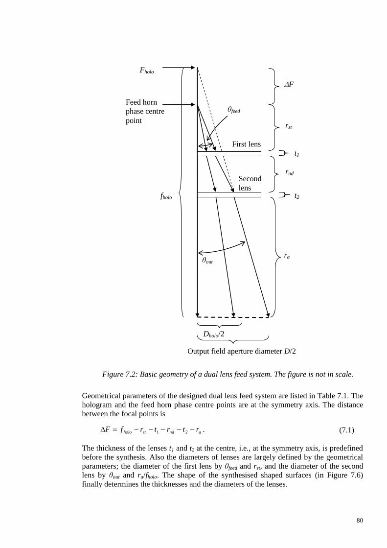
7.1.1 Geometry ...................................................................................................79
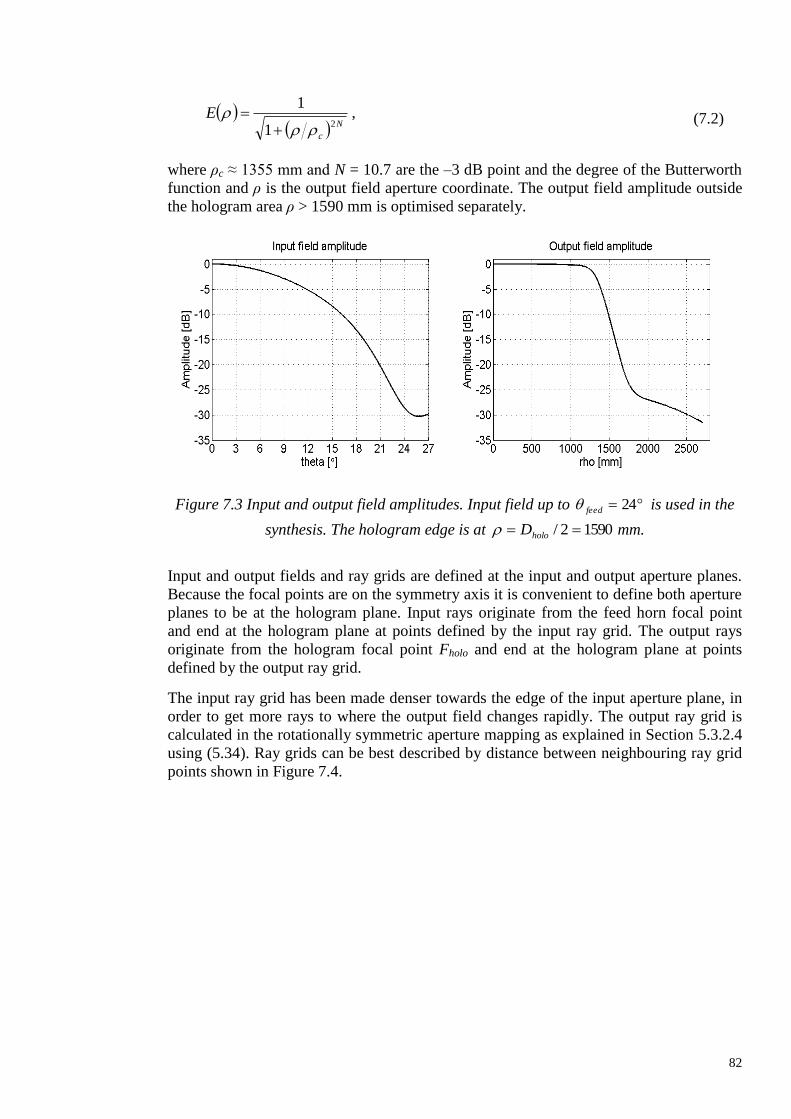
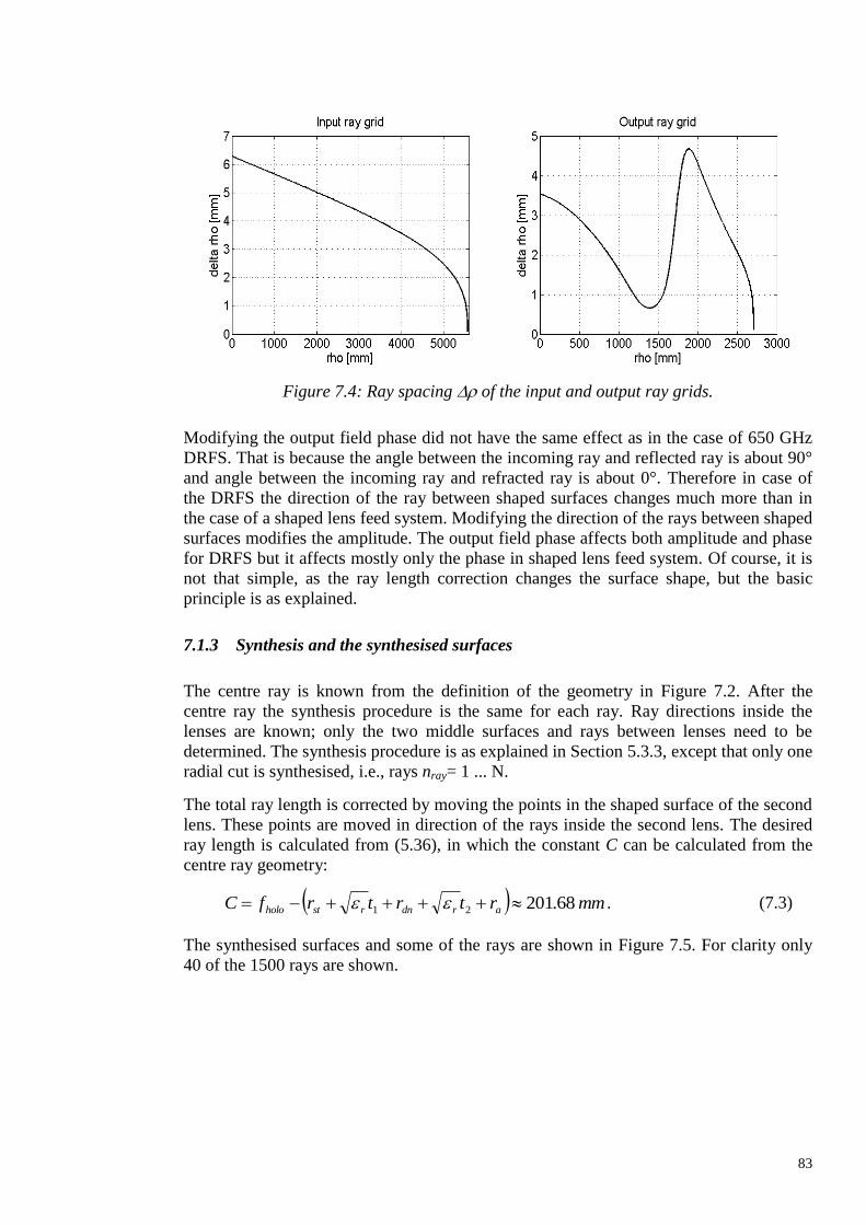
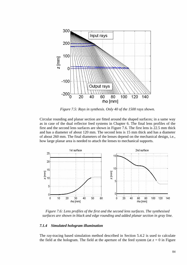
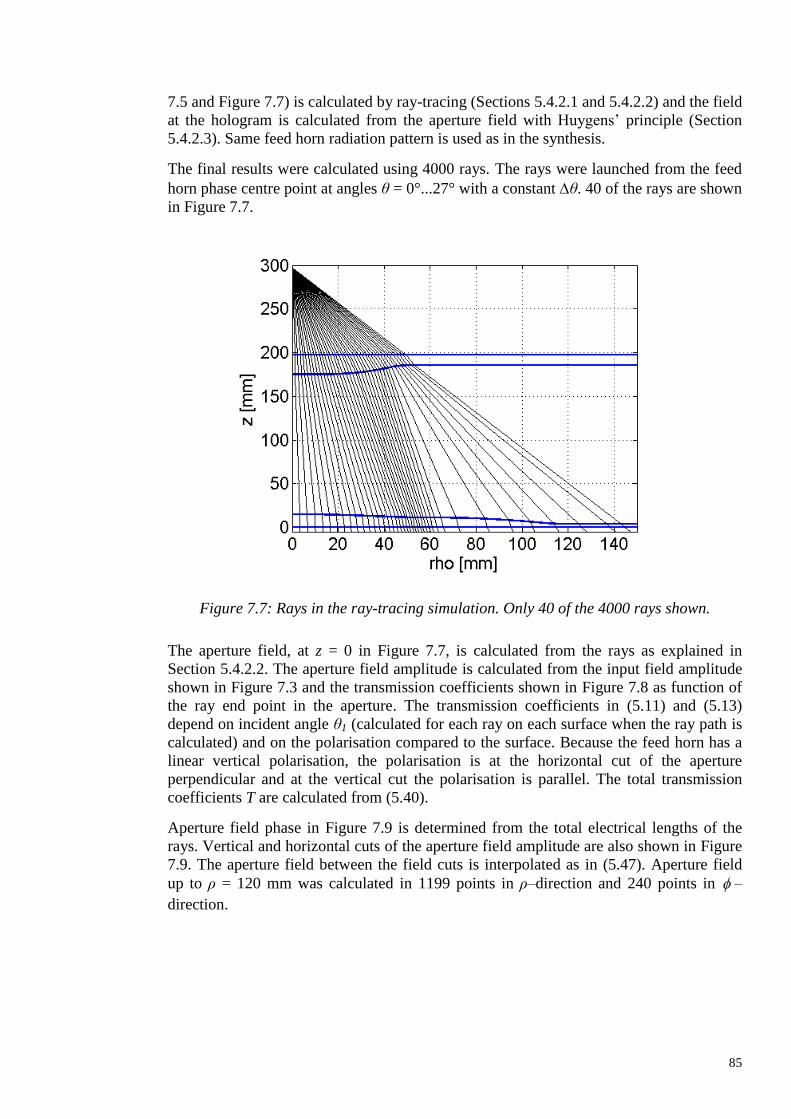
7.1.2 Input and output fields in synthesis...........................................................81 7.1.3 Synthesis and the synthesised surfaces .....................................................83 7.1.4 Simulated hologram illumination..............................................................84
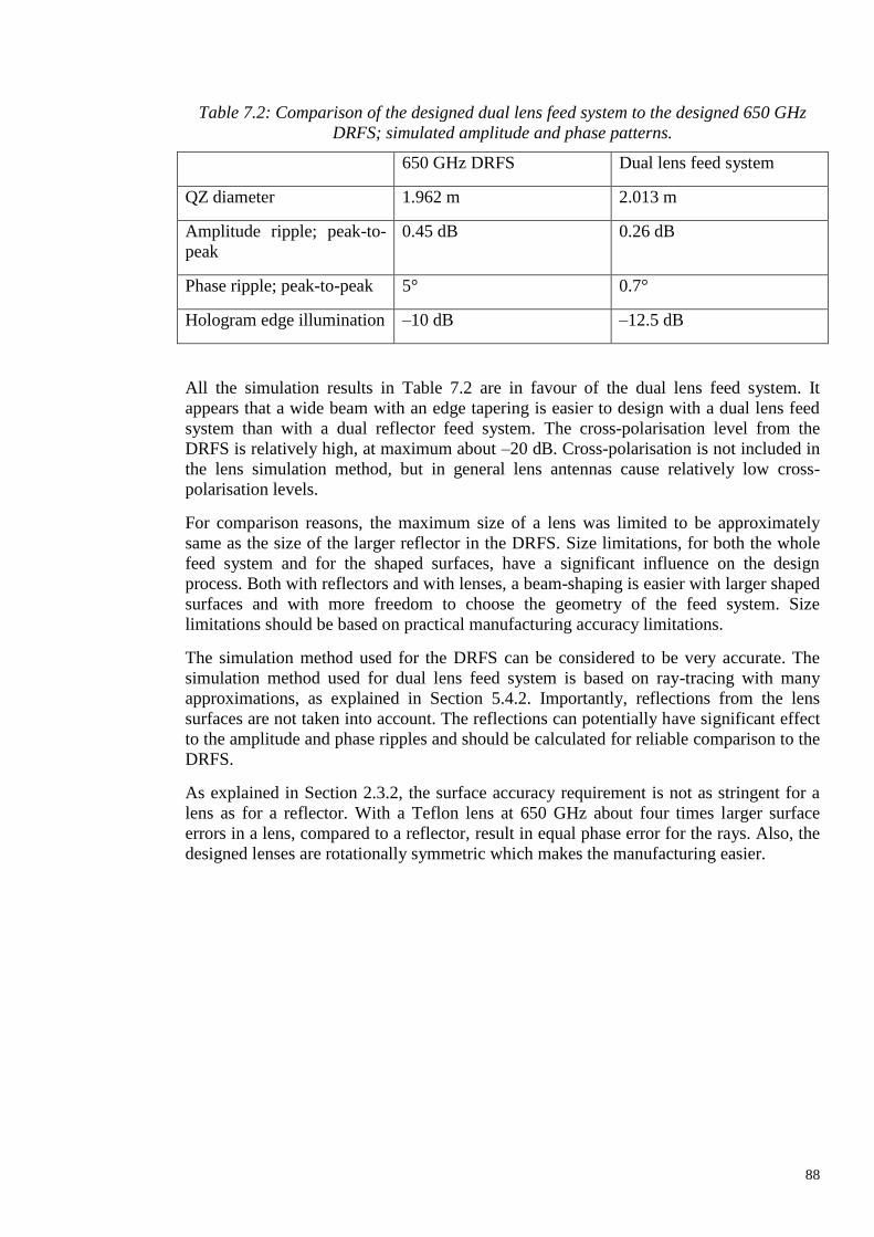
7.1.5 Comparison to the 650 GHz DRFS...........................................................87
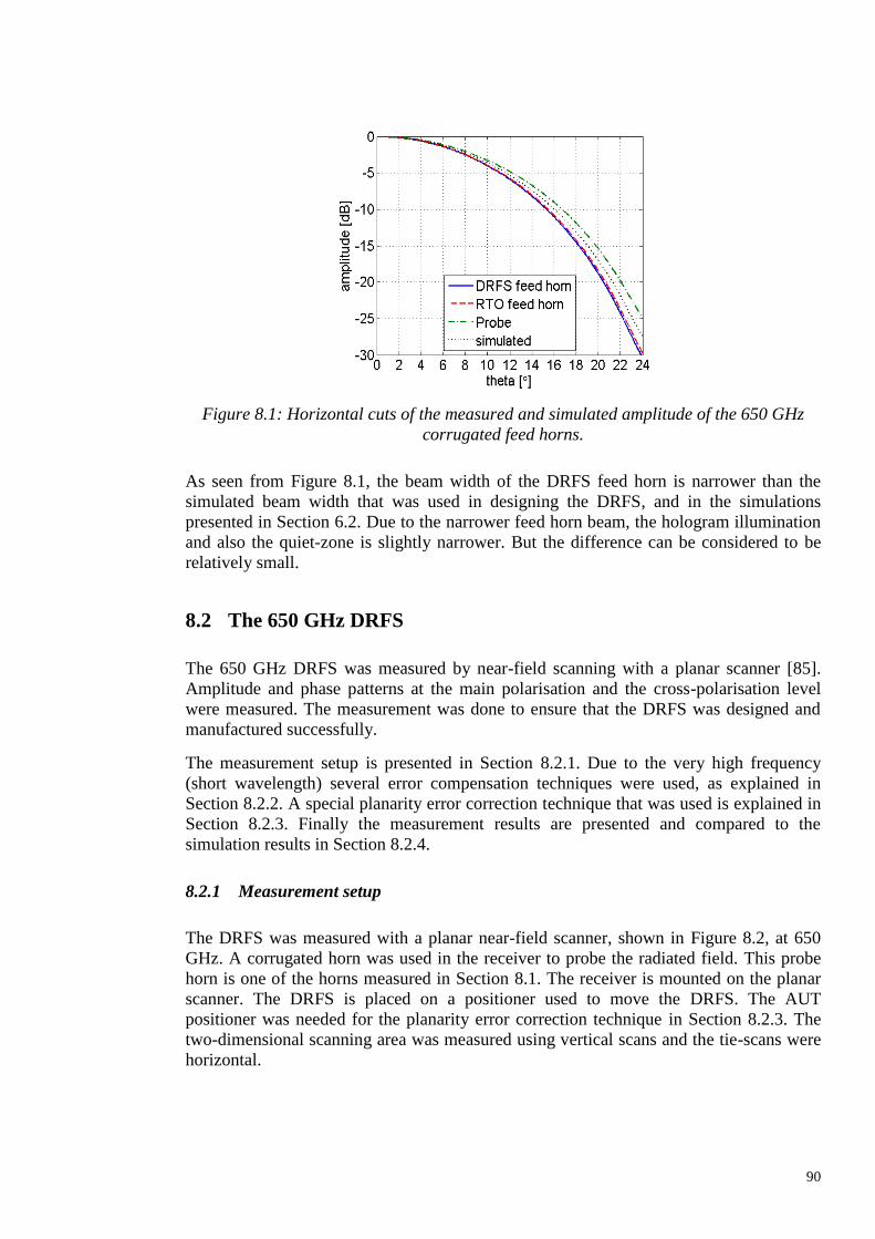
8 Measurements ......................................................................................................89 8.1 The 650 GHz feed horns ..................................................................................89
8.2 The 650 GHz DRFS .........................................................................................90
8.2.1 Measurement setup ...................................................................................90 8.2.2 Error compensation techniques .................................................................91 8.2.3 Planarity error correction technique ..........................................................92 8.2.4 Measurement results of the 650 GHz DRFS .............................................94
8.3 Hologram-based CATR at 650 GHz ................................................................95
9 Conclusions ...........................................................................................................97
References ...................................................................................................................99
Page 7
7
List of symbols
a Index
b Index
e Eccentricity
em Eccentricity of a main reflector
es Eccentricity of a subreflector
fholo Hologram focal length
fsub Subreflector focal length
i Index
j Imaginary unit
k Wave number, index
k0 Wave number in free-space
k Local wave vector, wave vector
l Length, index
mray Number of the ray
mtube Number of the ray tube
n Index of refraction, index
nray Number of the ray
ntube Number of the ray tube
n Normal vector
r Distance, far-field criterion, spherical coordinate
rmain Main reflector distance from the output aperture
rsub Distance between reflectors
r Vector, direction, position
s Distance along a ray
t Time, thickness
t Tangential vector, tangential unit vector of a ray
u Unit vector
iu Unit vector in direction i
x, x’ Cartesian coordinate
y, y’ Cartesian coordinate
z, z’ Cartesian coordinate, cylindrical coordinate
A Area, number of points
B Number of points
C Constant
D Diameter of an antenna, diameter of an aperture
Dholo Diameter of a hologram
Page 8
8
0, EE Electric field
Ea Electric field strength in aperture
Eh Electric field strength of hologram illumination
aE Electric field in aperture
hE Electric field in hologram illumination
POE Electric field calculated with PO
PTDE Electric field calculated with PTD
F Focal point, phase centre point
F Function
Ffeed Focal point of a feed
Fholo Focal point of a hologram
Fmain Focal point of a main reflector
G Green’s function
G Green’s dyad
H Magnetic intensity
aH Magnetic intensity in aperture
iH Incident magnetic intensity
J Electric current density
mJ Magnetic current density
msJ Magnetic surface current density
sJ Electric surface current density
K Number of points
L Eikonal function, number of points
M Number of rays in a ray ring
N Number of ray rings, degree of Butterworth function
Nsurf Number of surfaces
P Power
R Distance, radius
S, S’ Surface
T Total transmission coefficient
α Scaling factor, angle between axis
αfeed Feed offset angle
αsub Subreflector offset angle
β Angle between axis
Permittivity
0 Permittivity of free-space
Page 9
9
r Relative permittivity
η Wave impedance
η0 Wave impedance in free-space
θ Angle
θfeed Feed horn half-beam width
θmain Output half-beam width
λ Wavelength
Permeability
0 Permeability of free-space
r Relative permeability
ρ Cylindrical coordinate, reflection coefficient
ρc Half power (–3 dB) point of Butterworth function
σ Conductivity
σm Magnetic conductivity
τ Transmission coefficient
Cylindrical coordinate
Angular frequency
Phase
Page 10
10
List of abbreviations
AUT Antenna under test
CATR Compact antenna test range
DRFS Dual reflector feed system
ESA European space agency
FDTD Finite-difference time-domain
GA Genetic algorithm
GO Geometrical optics
JAXA Japan aerospace exploration agency
NASA National aeronautics and space administration
NICT National institute of information and communications technology
NURBS Non-uniform rational B-spline
PEC Perfect electric conductor
PMC Perfect magnetic conductor
PO Physical optics
PTD Physical theory of diffraction
QPS Quintic pseudosplines
RAM Radar absorbing material
RCS Radar cross-section
RTO Representative test object
TE Transverse electric
TKK Teknillinen korkeakoulu (Helsinki University of Technology)
TM Transverse magnetic
QZ Quiet zone
Page 11
11
1 Introduction
Large millimetre and submillimetre wave antennas are used to study the earth and the
universe at millimetre and submillimeter wavelengths. Several ongoing space research
projects will study the universe at submillimetre wavelengths, e.g., Herschel (ESA) [1],
[2], Planck (ESA) [1], [2], SPIRIT (NASA) [3], and SPECS (NASA) [3]. Examples of
missions to study the atmosphere at submillimetre wavelengths are EOS MLS (NASA)
[4], and SMILES (NICT, JAXA) [5], [6]. Electrically large reflector antennas are needed
for high angular resolution. Accurate manufacturing of the reflector is very difficult and
therefore the operation of the antenna should be verified with measurements prior to the
launch.
A compact antenna test range (CATR) is best suited for testing large antennas at high
frequencies. In a CATR, the far-field conditions, i.e., a quiet zone (QZ), needed for
testing the antenna under test (AUT), are created with a collimating element.
Conventionally, the collimating element in a CATR is a reflector or a set of reflectors.
The highest usable frequency of a reflector-based CATR is typically limited by the
surface accuracy of the reflectors.
MilliLab at TKK Helsinki University of Technology has developed a hologram-based
CATR since the 1990’s [7], [8]. A hologram-based CATR can be used to test large
antennas at millimetre [9], [10] and submillimetre wavelengths [11], [12]. The hologram
is a light weight planar structure and therefore much easier and cheaper to manufacture
than the large reflectors in the conventional CATRs.
Traditionally a corrugated feed horn has been used to illuminate the hologram. Because
of the high edge illumination, narrow slots have been needed at the edges of the
hologram. These narrow slots are difficult to manufacture accurately and limit the use of
the hologram to a polarisation parallel to the slots, i.e., the vertical polarisation. The
narrow slots can be avoided by using shaped illumination of the hologram. The shaped
illumination can be realised by designing a feed system that modifies both amplitude and
phase pattern of the primary feed, i.e., a corrugated feed horn.
A dual reflector feed system (DRFS) can be used as a feed system for a hologram-based
CATR [13], [12]. Previously, a 310 GHz DRFS for hologram-based CATR has been
demonstrated at 310 GHz [14]. A numerical ray-tracing based synthesis method [15],
[13] was developed specifically for this purpose. Later, a 650 GHz DRFS [16], [17] was
designed as part of a large antenna measurement project [12]. Same ray-tracing principles
can be used to design a feed system based on shaped lenses.
In this thesis, the design principle of the feed systems for hologram-based compact ranges
is presented. The synthesis method and design procedure, used to design the dual
reflector feed systems, is generalised also for shaped lens feed systems. The 650 GHz
DRFS and a design example of a shaped lens feed system are presented in detail.
Page 12
12
2 Antenna measurement techniques
Antenna measurement techniques can be divided into three basic types: far-field
measurements, near-field scanning techniques and compact antenna test ranges (CATR).
In general, antenna measurement aims at determining the antenna radiation pattern. Also,
for example, antenna impedance, radiation efficiency, etc. can be measured.
Antenna pattern includes relative amplitude, relative phase, polarisation, and the power
gain [18]. Often antenna pattern is expressed as amplitude and phase patterns for main
and cross-polarisations.
Far-field and near-field measurements are briefly explained in Sections 2.1 and 2.2,
respectively. In Section 2.3 compact antenna test ranges are explained.
Antenna measurement results of this thesis are in Chapter 8. Many different antenna
measurement techniques are used. In Section 8.1, the 650 GHz feed horns are measured
in the far-field of the AUT. In Section 8.2, the 650 GHz DRFS is measured by near-field
scanning. In Section 8.3, the 650 GHz DRFS is used in a compact antenna test range and
the quiet-zone quality is tested with near-field scanning.
2.1 Far-field measurement
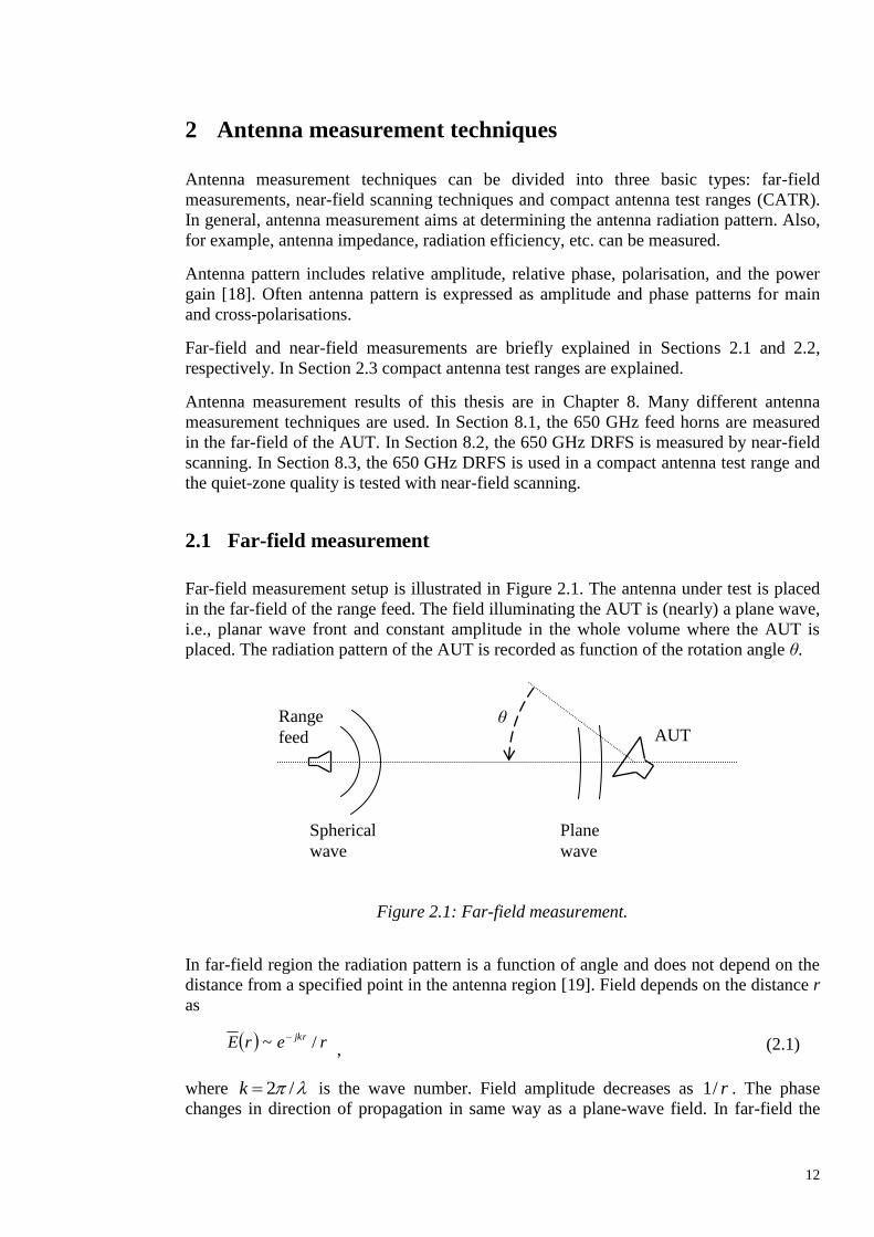
Far-field measurement setup is illustrated in Figure 2.1. The antenna under test is placed
in the far-field of the range feed. The field illuminating the AUT is (nearly) a plane wave,
i.e., planar wave front and constant amplitude in the whole volume where the AUT is
placed. The radiation pattern of the AUT is recorded as function of the rotation angle θ.
In far-field region the radiation pattern is a function of angle and does not depend on the
distance from a specified point in the antenna region [19]. Field depends on the distance r
as
rerE jkr /~
, (2.1)
where /2k is the wave number. Field amplitude decreases as r/1 . The phase
changes in direction of propagation in same way as a plane-wave field. In far-field the
Range
feed AUT
Spherical
wave
Plane
wave
θ
Figure 2.1: Far-field measurement.
Page 13
13
ratio of electric and magnetic field is a constant called a wave impedance η. In vacuum
(and in air) η0 ≈ 377 . The electric and magnetic fields are orthogonal to each other and
to the direction of propagation.
Typically far-field criterion is defined as:
22Dr
, (2.2)
where D is the diameter of the antenna and is the wavelength. The far-field criterion is
defined as the distance from the antenna where the distance to the edge of the antenna is
/16 longer than the distance to the centre of the antenna, i.e., phase deviation from a
plane wave is 22.5. For example, if the first side lobe is at –40 dB then side lobe level
measurement error is 1 dB at a distance of /6 2D [20].
At sub-millimetre wavelengths for a large antenna the far-field criterion can be tens of
kilometres and atmospheric attenuation is very high; therefore far-field measurements can
be impossible. For example, the far-field criterion (2.2) gives about 10 km for a 1.5 m
diameter antenna at 650 GHz. Far-field measurements are possible for small antennas, as
for example the far-field criterion is only about 4 cm for a 3 mm diameter antenna at 650
GHz.
The 650 GHz feed horns, in Section 8.1, are measured in the far-field of the AUT. Instead
of rotating the AUT, the radiation pattern is measured with a planar scanner. The
measurement distance of about 1 m is clearly in the far-field region. A so-called three
antenna method is used to measure the beam widths of the three feed horns.
2.2 Near-field measurement
In near-field antenna measurements the antenna radiation is measured in the near field
and the far-field radiation is calculated from the near-field data for example using the
Fourier-transform. The near field is sampled with a probe antenna on a surface in the
radiating near-field of the AUT. The sampling surface can be planar, spherical or
cylindrical.
The sampling interval has to be smaller than /2 for the full angular coverage [21] and
position accuracy better than /100. The measurements of large high frequency antennas
are very challenging because of the required high dynamic range, probe position accuracy
and very high number of sampling points.
Example of near-field measurements at frequencies up to 650 GHz is in [22]. A very high
precision granite scanner mechanism was used to achieve the required planar accuracy.
Error sources in near-field measurement are analysed for example in [23], [24]. Error
analysis of a near-field measurement system is in general a combination of closed-form
equations, simulations, and measurement tests.
In planar near-field measurements the planarity error of the scanner can be very
significant error source. Planarity errors can affect the measured phase significantly at
high frequencies as the planarity affects directly the measurement distance, i.e., the
Page 14
14
electrical path length. The phase error yx, caused by planarity error yxz , can be
expressed simply as:
360,
,
yxzyx . (2.3)
Equation (2.3) is valid only for incident plane wave but can be used also for incident
spherical wave if the resulting path length error is small (incident angle is small).
Planarity errors can be corrected from the measurement results if the planarity of the
scanner is known.
The 650 GHz DRFS is measured by near-field scanning in Section 8.2. The far-field
pattern was not calculated as the DRFS is used in the near-field region (far-field criterion
gives a few hundred meters and the distance to the hologram is 12.72 m). Averaging of
measurements, drift compensation with tie-scans, probe correction, and a planarity error
correction techniques were used to reduce the measurement errors.
2.3 Compact antenna test range
Compact antenna test range (CATR) is based on using a collimating element that creates
the needed far-field conditions for the antenna measurement. The area where the far-field
conditions are created is called the quiet zone (QZ). The antenna under test (AUT) is
rotated as in the far-field measurements and the radiation pattern is recorded. The
collimating element can be a reflector, a set of reflectors, a lens, or a hologram. Compact
ranges can also be used in radar cross-section (RCS) measurements.
The development of CATRs started in 1950’s with lenses [25], [26]. The reflector based
CATRs have been developed since the 1960’s [27], [26]. A hologram-based CATR was
first proposed in 1992 [7].
Main advantage of a CATR is that the measurements can be done inside in controlled
environment in relatively small space. Also, there is no need to calculate near to far-field
transformation as in the near-field measurements. Usually ripple of 1 dB peak-to-peak
and 10° peak-to-peak is allowed at maximum in the quiet-zone field amplitude and phase,
respectively.
2.3.1 Reflector-based compact antenna test range
The most common CATR is based on a reflector or a set of reflectors. Reflector based
compact antenna test ranges are commonly used at frequencies up to 200 GHz [28], [29].
A reflector-based CATR has been used in antenna test up to 500 GHz [30]. The highest
usable frequency of a reflector-based CATR is typically limited by the surface accuracy
of the reflectors. The surface accuracy requirement is approximately λ/100 [18]. The
lowest usable frequency is limited by the diffracted fields from the edges of the reflectors
as the diffracted fields are strongest at low frequencies [26].
The main reflector has to be larger than the quiet-zone. The quiet-zone diameter is
typically about 1/3 of the main reflector diameter for a single reflector CATR and 2/3 for
dual reflector CATR. Reflector geometries used are: a single offset reflector [27], a dual
Page 15
15
cylindrical reflector [32], a dual offset reflector [29], [33], [34] and a triple offset
reflector [35], [36]. Examples of CATR geometries are illustrated in Figure 2.2.
Offset paraboloidal reflectors produce typically about –30 dB cross-polarisation level to
the QZ [26]. The cross-polarisation performance can be improved by using two reflectors
and by choosing the parameters of the CATR so that the cross-polarisation is minimised
[37], [38]. Examples of cross-polarisation compensated CATRs are in [29], [33].
Diffraction from the reflector edges causes ripples to the QZ. The edge diffraction can be
reduced with reflector edge treatment, e.g. serrations [39], rolled edge [39], or by
reducing the edge illumination by shaping the reflectors [34], [35].
2.3.2 Lens-based compact antenna test range
A lens can be used as a collimating element in a CATR. Geometry of a classical lens-
based CATR is presented in Figure 2.3 [40]. The lens is designed to correct the phase
pattern of the range feed to a plane wave. In [41], plastic foam lens is used with added
loss into the lens so that also the amplitude is nearly uniform behind the lens.
Advantages of the lens-based CATR are [26]: high utilisation factor (ratio of diameter of
the collimating element to the diameter of the QZ), low cross-polarisation level, and that
there is no direct radiation from the feed to the QZ. Disadvantages are [26]: amplitude
taper (due to feed horn amplitude pattern and transmission coefficient at larger incident
angles), relatively long length, and the need to achieve homogeneity in the dielectric.
Feed horn
Paraboloid
Feed horn
Subreflectors
Spherical main reflector
Figure 2.2: Examples of a single offset reflector and a trireflector CATR.
Page 16
16
Figure 2.3: Geometry of a classical lens-based CATR designed for radar cross-section
(RCS) measurements [40].
Lens-type compact antenna test range at mm-waves is studied in [42], in which the lens
shape is calculated with a ray-tracing method presented in [43].
Compact antenna range based on a lens is mainly potential at very high frequencies as the
surface accuracy requirement for a reflector becomes too stringent. Because a lens is a
transmission-type element and because the wave length is shorter inside the lens, the
surface accuracy requirement is weighted by 21r compared to a reflector [42].
r is the relative permittivity of the lens material. The difference of the effect of a surface
error is illustrated in Figure 2.4.
Figure 2.4: The effect of a surface error in case of a reflector and in case of a lens [42].
Page 17
17
2.3.3 Hologram-based compact antenna test range
A computer-generated radio-wave hologram can be used as a collimating element in a
compact antenna test range [8]. The hologram is an interference pattern of the wave-front
illuminating the hologram and the desired goal field [44]. In a CATR, the goal field is a
plane wave in the quiet zone.
Antenna tests that have been done in hologram-based CATRs are listed in Section
2.3.3.1. All holograms used in antenna tests have been transmission-type amplitude
holograms. Also, phase holograms [45], [46], and reflection-type holograms [47] have
been studied.
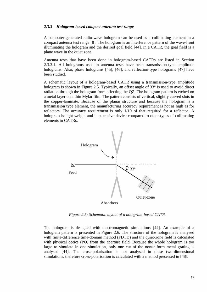
A schematic layout of a hologram-based CATR using a transmission-type amplitude
hologram is shown in Figure 2.5. Typically, an offset angle of 33° is used to avoid direct
radiation through the hologram from affecting the QZ. The hologram pattern is etched on
a metal layer on a thin Mylar film. The pattern consists of vertical, slightly curved slots in
the copper-laminate. Because of the planar structure and because the hologram is a
transmission type element, the manufacturing accuracy requirement is not as high as for
reflectors. The accuracy requirement is only 1/10 of that required for a reflector. A
hologram is light weight and inexpensive device compared to other types of collimating
elements in CATRs.
The hologram is designed with electromagnetic simulations [44]. An example of a
hologram pattern is presented in Figure 2.6. The structure of the hologram is analysed
with finite-difference time-domain method (FDTD) and the quiet-zone field is calculated
with physical optics (PO) from the aperture field. Because the whole hologram is too
large to simulate in one simulation, only one cut of the nonuniform metal grating is
analysed [44]. The cross-polarisation is not analysed in these two-dimensional
simulations, therefore cross-polarisation is calculated with a method presented in [48].
Absorbers
Feed
Quiet-zone
Hologram
33º
Figure 2.5: Schematic layout of a hologram-based CATR.
Page 18
18
Figure 2.6: Example of a transmission-type amplitude hologram pattern. Metal is in
black and slots in white.
A transmission-type hologram can be an amplitude hologram or a phase hologram. In an
amplitude-type hologram the radiation is partially blocked by metal strips and partially
transmitted through slots between the metal strips. A phase hologram is based on locally
varying the effective electrical path length, for example by varying the effective thickness
pattern. A phase hologram can be realized by milling grooves on a dielectric substrate
[45]. With a phase hologram it is possible to have higher conversion efficiency, i.e.,
lower losses.
A phase hologram has been used in a hologram-based compact radar cross section (RCS)
range for scale model measurements at 310 GHz [45]. The layout of the RCS range is
similar to the layout in Figure 2.5. The scale model is placed in the QZ and the
transmitter and receiver are separated with a dielectric slab working as a directional
coupler.
A reflection-type phase hologram CATR has also been designed [47]. In a reflection-type
phase hologram grooves are milled into a metal slab. The main advantages compared to
transmission-type holograms are lower losses and that the harmful reflections inside the
hologram are avoided.
2.3.3.1 History of antenna tests in a hologram-based CATR
Hologram-based CATRs have been used in antenna tests at frequencies from 39 GHz up
to 650 GHz [9]–[12].
In [9], a planar antenna made of array of waveguide fed horns [49] is measured in a
hologram CATR at 39 GHz. The QZ is measured to be 70 cm × 45 cm. The same antenna
was measured also with near-field scanning and with conventional far-field technique and
Page 19
19
the measurement results are found to agree well down to side-lobe levels 30–35 dB below
peak [9].
Measurement of the Odin telescope [50] at 119 GHz is presented in [10]. The Odin
telescope has a 1.1 m offset reflector antenna shown in Figure 2.7. The 2.4 m × 2.0 m
hologram produces about 1.65 m × 1.55 m QZ. The measured main lobe is symmetric
and the beam-width is as designed [10].
Figure 2.7: The 1.1 m offset reflector antenna on the Odin satellite [10].
A 1.5 metre diameter antenna was measured at 322 GHz in 2003. The design and
construction of the CATR and the QZ tests are presented in [51]. The antenna test results
are presented in [11]. The antenna under test was ADMIRALS representative test object
(RTO) [30]. A photograph of the RTO is in Figure 2.8. The 3-m-diameter hologram is
soldered together from three separate pieces. The measured antenna radiation pattern
corresponds reasonably well to the simulated pattern. The effect of the non-ideal quiet-
zone field on the measured radiation pattern was investigated by computing the radiation
of the simulated antenna including the effect of the measured quiet-zone field in [11].
Page 20
20
Figure 2.8: ADMIRALS RTO on the antenna positioner [11].
In 2006, the ADMIRALS RTO was tested at 650 GHz in a hologram-based CATR [12].
This is the highest frequency at which a large antenna has ever been measured in any
CATR. The hologram diameter is 3.16 m. A DRFS is used to provide a modified
illumination for the hologram for a first time in an antenna measurement. The range feed,
i.e., the DRFS, is placed 12.72 m from the hologram and the AUT is placed about 9 m
from the hologram. Layout of the CATR is shown in Figure 2.9.
Figure 2.9: Layout of the CATR [12].
Page 21
21
2.3.3.2 Feed system for a hologram-based CATR
Traditionally a corrugated feed horn has been used to illuminate the hologram [9], [10],
[11]. This leads to high edge illumination of the hologram and the slots in the hologram
pattern need to be narrowed towards the edges to reduce the ripple caused by edge
diffractions.
Traditionally the holograms have been limited to be used only at the linear vertical
polarisation. That is because transmission of a horizontal polarisation through the vertical
slots is nearly independent of the slot width [52]; and therefore edge diffraction at the
horizontal polarisation is not avoided with the narrowing of the slots.
The narrow slots are also difficult to manufacture accurately. It may happen that the
narrow slots are not completely etched and that reduces the hologram size and increase
edge diffraction [44].
The narrow slots can be avoided if the hologram is illuminated with a modified
illumination. For example, a dual reflector feed system (DRFS) can be used to modify the
hologram illumination [14], [17]. The hologram illumination can be designed to have a
flat amplitude to the centre of the hologram and amplitude tapering to the edge of the
hologram. Hologram designed for such modified illumination does not need to change
the amplitude distribution and therefore the narrow slots can be avoided. The hologram is
only used to transform the spherical phase front to a planar one [44]. Avoiding the narrow
slots has several advantages.
An example of slot widths of holograms designed for a modified illumination and for the
traditional Gaussian illumination is shown in Figure 2.10.
Figure 2.10: Example of slot widths of a 310 GHz holograms along the centreline
designed for modified illumination (from DRFS) or for a traditional Gaussian
illumination [53].
The advantages of using the modified illumination are listed in the following paragraphs.
1) The slots in the hologram pattern can be wider and the slot widths can be almost
uniform which simplifies the manufacturing of the hologram.
2) The hologram can be optimised for both vertical and horizontal polarisations [53].
Page 22
22
3) The hologram can be designed to operate almost identically at both linear
polarisations [52]. Hologram that operates identically at both linear polarisations
could be used to test antennas at circular polarisation.
4) Cross-polarization in the QZ with a hologram designed for a corrugated feed horn
is from –15 dB to –20 dB [44], [48]. By using the modified illumination the cross-
polarisation performance of the hologram is improved by about 10 dB [52],
without taking into account the cross-polarisation in the illuminating field. If the
feed system provides sufficiently low cross-polarisation level, the cross-
polarisation in the QZ can be reduced by using a modified illumination from a
feed system.
5) The quiet-zone size is in practice determined by the –1 dB beam width of the
hologram illumination [13], [44]. The QZ diameter is approximately cos(33°)
times the –1 dB beam width in the horizontal direction because of the offset
angle. By designing a feed system with wider beam width it is possible to increase
the QZ to hologram size ratio.
Amplitude and phase ripples in the illumination increase directly the overall ripples in the
quiet-zone field. QZ field ripples are a combination of ripples in the illumination and
ripples caused by the hologram. The ripples in the illuminating field should be as small as
possible.
Two dual reflector feed systems have been made; one at 310 GHz [13], [14] and one at
650 GHz [16], [17]. The numerical synthesis method that is used to design feed systems
for hologram-based CATRs is presented in detail in Chapter 5. The designed DRFSs are
presented in Chapter 6. The same synthesis method is used for a feed system based on
shaped lenses in Chapter 7.
Page 23
23
3 Calculation of field radiated by an antenna
Calculation of field radiated by an antenna is always based on solving the Maxwell’s
equations [54]:
mJHjE (3.1)
JEjH , (3.2)
where E is the electric field, H is the magnetic field, J and mJ are the electric and
magnetic current densities, ω is the angular frequency, μ is permeability, and ε is
permittivity. Time dependence of tje is assumed. Sometimes the current densities are
known with good accuracy. For example for a dipole the current is known and the
radiated field can be calculated with Maxwell’s equations.
Often the antenna structure is too complex to directly determine the current densities. The
antenna structure can be replaced with equivalent current sources without changing the
radiated field. When the equivalent current sources are determined the radiated field can
be calculated with Maxwell’s equations. There are many methods that can be used to
determine these equivalent current sources. Calculation of equivalent current sources
from a known aperture field, and calculation of radiated field from these currents, is
explained in Section 3.1.
If a field illuminating a known metal object (antenna) is known, the surface currents can
be calculated using physical optics (PO). PO is described in Section 3.2. Physical optics
does not take into account diffraction from edges of the antenna structure. Physical theory
of diffraction (PTD) can be used to include the diffracted fields to PO, as explained in
Section 3.3. PO (with PTD) is commonly used to analyse electrically large reflector
antennas. In this thesis, PO and PTD are used to simulate the radiated field of a dual
reflector feed systems (DRFS), as explained in Section 5.4.1.
Geometrical optics (GO) is a high frequency approximation of the Maxwell’s equations.
GO is commonly used to analyse lens and reflector antennas. The basic equations of
geometrical optics are introduced in Section 3.4. The numerical synthesis method used to
design feed systems for hologram-based compact ranges is a GO-based ray-tracing
synthesis method. The numerical synthesis method is explained in detail in Chapter 5. In
this thesis, field radiated by a shaped lens antenna is analysed by calculating the aperture
field with ray-tracing and the radiated field is calculated from the equivalent current
sources. This ray-tracing method is explained in Section 5.4.2.
The antenna radiation analysis methods used in designing the feed systems are described
in Sections 3.1–3.4.
3.1 Radiation of an aperture
Radiation of an aperture antenna can be calculated with Huygens’ principle [54].
Examples of aperture antennas are open-ended waveguide, horn antenna, and reflector or
lens antennas. According to Huygens’ principle sources inside a closed surface S can be
Page 24
24
replaced with surface sources sJ and msJ on the surface. These are called equivalent
sources (or Huygens’ sources) [19]. The equivalent surface currents depend on the
electric and magnetic fields on the surface as: [54], [55]
HnJ s (3.3)
EnJ ms , (3.4)
where n is the surface normal pointing out of the surface. The original antenna problem
can be replaced with these surface currents and air inside the closed surface S. Then the
field radiated by the antenna can be calculated with Maxwell’s equations with these
surface currents as sources.
The problem can be simplified if the volume inside S is filled with either perfect electric
(PEC) or perfect magnetic (PMC) conductor [54]. If the volume is filled with magnetic
conductor, with m ( ), msJ can be eliminated, and if the volume is filled with
electric conductor, with ( ), sJ can be eliminated. Therefore, it is necessary
to evaluate only either magnetic or electric field on the surface S and the sources are
calculated using either (3.3) or (3.4).
It is often convenient to define the surface S to be the aperture plane of the antenna. The
aperture plane divides the antenna problem into two half-spaces, one with the antenna
structure and sources and one source-free half-space where the field is calculated. If the
aperture plane is infinite it is a closed surface and Huygens’ principle applies.
For simplicity from now on we assume that the electric field on the aperture aE is
known, and the antenna problem is replaced with perfect electric conductor and
equivalent magnetic surface currents, as shown in Figure 3.1.
The method of images gives the equivalent surface currents on the surface S:
aE
HE, HE,
PEC
Aperture
ams
s
EnJ
J
2
0
Figure 3.1: The original antenna problem is replaced with perfect conductor
and equivalent magnetic surface currents.
Page 25
25
0sJ (3.5)
ams EnJ 2 . (3.6)
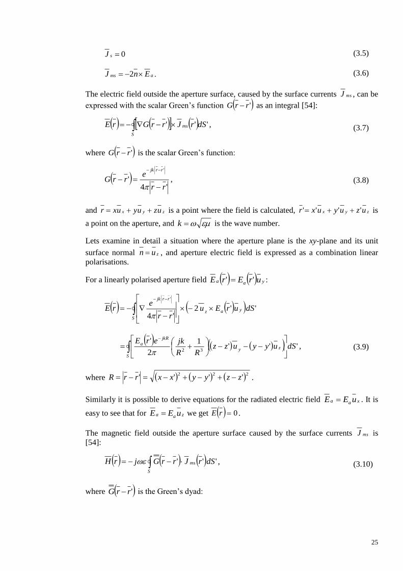
The electric field outside the aperture surface, caused by the surface currents msJ , can be
expressed with the scalar Green’s function 'rrG as an integral [54]:
S
ms dSrJrrGrE ''' , (3.7)
where 'rrG is the scalar Green’s function:
'4
'
'
rr
errG
rrjk
, (3.8)
and zyx uzuyuxr is a point where the field is calculated, zyx uzuyuxr '''' is
a point on the aperture, and k is the wave number.
Lets examine in detail a situation where the aperture plane is the xy-plane and its unit
surface normal zun , and aperture electric field is expressed as a combination linear
polarisations.
For a linearly polarised aperture field yaa urErE '' :
S
yaz
rrjk
dSurEurr
erE ''2
'4
'
S
zy
jkR
a dSuyyuzzRR
jkerE'''
1
2
'32
, (3.9)
where 222'''' zzyyxxrrR .
Similarly it is possible to derive equations for the radiated electric field xaa uEE . It is
easy to see that for zaa uEE we get 0rE .
The magnetic field outside the aperture surface caused by the surface currents msJ is
[54]:
S
ms dSrJrrGjrH ''' , (3.10)
where 'rrG is the Green’s dyad:
Page 26
26
'1'
2rrG
kIrrG
. (3.11)
Alternatively, if the volume inside S is filled with magnetic conductor the surface
currents sJ are calculated by the method of images and 0msJ . The electric and
magnetic fields caused by the surface currents sJ are: [54]
S
s dSrJrrGjrE ''' (3.12)
S
s dSrJrrGrH ''' . (3.13)
In far-field 'rr and the distance from field point to integration point 'rr can be
approximated: (with first two terms of Taylor series)
'' rurrr r . (3.14)
The far-field approximation of the Green’s function is: [54]
'
4
rujkjkr
rer
eG
, (3.15)
and the approximation of the Green’s dyad is: [54]
r
euuIG
jkr
rr
4
, (3.16)
where rurr , r is the distance from the antenna, and ru is the direction from the
antenna to the field point. The far-field is calculated from (3.7), (3.10), (3.12), or (3.13),
using the far-field approximation of the Green’s function (3.13) or Green’s dyad (3.16).
In far-field the relation of electric and magnetic fields is:
ruHE (3.17)
EuH r
1. (3.18)
3.2 Physical optics
Field reflected by a reflector can be calculated using physical optics (PO). Physical optics
is an approximation of surface currents. The physical optics approximation is valid for
scatterers made of perfect electric conductor that are large in terms of wavelengths [56].
In PO, the surface currents on a reflector surface are calculated from the incident field.
Reflected fields are calculated from these surface currents. Using Huygens’ principle, as
Page 27
27
explained in Section 3.1, the antenna structure can be replaced with perfect electric or
magnetic conductor and equivalent surface currents.
The surface is assumed locally flat and infinite. Surface current densities on a perfect
electric conductor are [54], [56]
is HnJ 2 (3.19)
0msJ , (3.20)
where n is the surface normal pointing out of the surface and iH is the incident
magnetic field. In the shadow region, i.e., surface area that is not directly illuminated by
the incident field, the surface currents are assumed to be zero. The reflected fields are
calculated with (3.12) and (3.13).
The surface currents are calculated in discrete points on the antenna surface [56]. At these
points the surface is approximated with the tangential plane and surface currents are
calculated from (3.19). In order to get sufficient accuracy with this approximation the
dimensions and radius of curvature have to be at least a few wavelengths. The number of
current elements has to be large enough for the PO to give accurate prediction of the
reflected field. The required number of the current elements depends on the size and the
shape of the object compared to the wavelength and the desired field accuracy.
3.3 Physical theory of diffraction
Physical theory of diffraction (PTD) can be used to include edge diffractions to PO [56].
In PTD edge currents are calculated from the shape of the edge and the incident field.
The field calculated from edge current is added to PO fields
PTDPO EEE . (3.21)
In the edge current calculations the edge is approximated locally to be a perfectly
conducting half plane. The radius of curvature of the edge and the number of current
elements has to be sufficiently large for this approximation to be valid. The PTD field is
calculated by integrating over the illuminated part of the edge from PTD equivalent edge
currents. These currents are calculated from fringe wave currents along incremental steps
on the edge [56]. A closed form expressions for PTD equivalent edge currents are derived
for truncated incremental wedge strips in [57].
3.4 Geometrical optics
Geometrical or ray optics is widely used in design of electrically large lens and reflector
antennas. The theory is explained in detail for example in [58], [55] (in English) or in
[54] (in Finnish).
Geometrical optics (GO) is a high frequency approximation of the Maxwell equations.
The high frequency approximation is accurate if all distances, radii of curvature, etc. are
large compared to the wavelength. The electric and magnetic fields can be expanded as
power series of inverse powers of the angular frequency [55]
Page 28
28
0
0,i
i
irLjk
j
rEerE
(3.22)
0
0,i
i
irLjk
j
rHerH
, (3.23)
where rL is the so called eikonal function and 000 k . At high frequencies the
0th
order dominates. The 0th
order equations describe the geometrical optics field:
0
0
0 Hk
LE
(3.24)
0
0
0 Ek
LH
(3.25)
00 LE (3.26)
00 LH . (3.27)
The geometrical optics field vectors rE 0 , rH 0 and rLkrk 0 are perpendicular
to each other. The surface where the phase is constant is given by the surface where
LRe is constant. When L is real power propagates in the direction of k , i.e.,
perpendicular to the constant phase front. The eikonal function determines the ray
directions and the wave fronts. The eikonal function is determined from the so the called
eikonal equation:
rnrrrLrL rr
2 , (3.28)
where rrrn rr is the index of refraction of the medium.
The ray equation represents the direction of propagation. For a ray )(sr the ray equation
derived from the eikonal equation is [54]:
rnds
rdrn
ds
dtnt
, (3.29)
where t is the tangential unit vector of the ray and s is the distance along the ray. The ray
equation is a second order non-linear differential equation. It can be solved analytically
for some cases, but usually it is solved numerically.
Field amplitude is calculated from the transport equation [54]:
Page 29
29
000
2
1E
nt
nEnt
nds
Ed
r
r
. (3.30)
The transport equation is a differential equation for an unknown vector 0E . If 0E is
known at some point it can be solved at all points along the ray. It can be proved from
(3.30) that 2
0E integrated over the cross-section of a ray tube is constant. Power
propagates inside the ray tube and the power density depends on the cross-sectional area
of the ray tube. Also polarisation and phase along the ray can be calculated from (3.30).
In geometrical optics the concept of rays is useful in understanding and illustrating the
propagation of geometrical optics fields. A ray is a line in space that represents the
direction of propagation. The ray path and field along the ray can be calculated. The
volume between rays is called a ray tube. Ray tubes are useful in understanding and
calculating propagation of power. In general, rays and ray tubes are used as conceptual
aid in deriving equations or functions that describe analytical solution to the given
problem. In general in geometrical optics, the properties of single rays are not calculated.
In ray-tracing fields are calculated by determining the path of a finite number of rays.
First rays are calculated from a known field and then these rays are traced one by one
(their path is calculated) through material, reflections, refractions, etc., and finally the
desired field is calculated from the resulting ray distributions, ray lengths, etc. Complex
systems can be analysed as it is not necessary to derive an analytical solution.
Page 30
30
4 Reflector and lens antennas
Large reflector and lens antennas are aperture antennas used to redirect the radiation of a
primary feed. Reflector and lens antennas are typically designed and analysed using GO
and PO [54]. The primary feed can be, e.g., a horn, a microstrip or a dipole antenna.
Reflector and lens antennas can be divided to common antenna types and to shaped
antennas. Reflector and lens antennas can also be divided to collimating and diverging-
beam antennas. High gain can be achieved with a collimating antenna. A feed system for
a CATR is an example of a diverging-beam shaped antenna [13], [16].
Common reflector antennas are presented in Section 4.1 and lens antennas in Section 4.2.
Synthesis methods for shaped antennas are presented in Section 4.4. The antenna type
and requirements for a feed system for hologram-type CATR are specified in Section 4.5.
4.1 Reflector antennas
Reflector antennas are widely used in telecommunication applications, radars, and radio
astronomy. Most high-gain antennas are reflector antennas. Reflector antennas are
secondary radiators, which redirect the radiation of the primary source, the feed. The feed
is usually a small horn antenna. Also feed arrays can be used. Reflector antenna has
usually one or two reflectors.
In general, the reflector can be of any shape but most reflector antennas are based on a
rotated conic section [59]: plane, hyperboloid, paraboloid, ellipsoid, or sphere. Properties
of rotated conic sections are discussed in Section 4.1.1. Also shaped reflectors are usually
based on these basic shapes and can be described as (nearly) planar, hyperbolical, etc.
In Section 4.1.2, collimating reflector antennas are presented. Collimating reflector
antennas are based on a parabolic reflector. Diverging-beam antennas based on
hyperboloids and/or ellipsoids are presented in Section 4.1.3.
4.1.1 Rotated conic sections
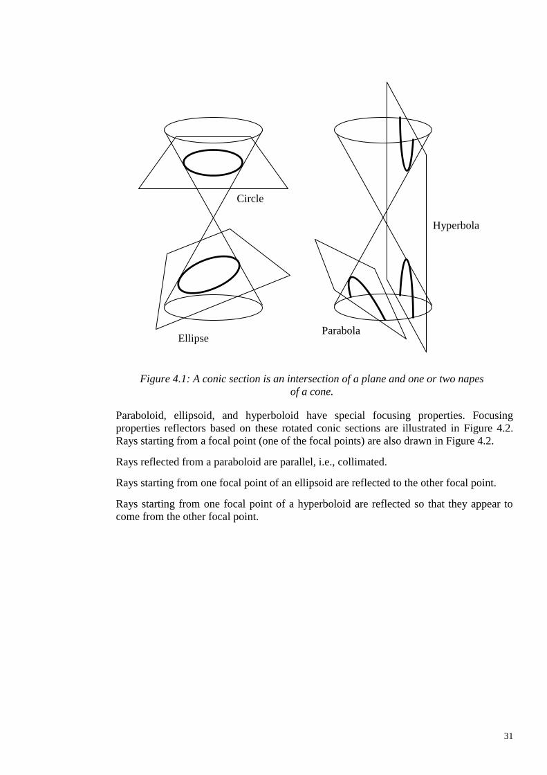
Many reflector antennas are based on rotated conic sections because of their geometrical
properties. An illustration of conic sections is in Figure 4.1. A line, a hyperbola, a
parabola, an ellipse, and a circle are special cases of a general conic section.
Page 31
31
Paraboloid, ellipsoid, and hyperboloid have special focusing properties. Focusing
properties reflectors based on these rotated conic sections are illustrated in Figure 4.2.
Rays starting from a focal point (one of the focal points) are also drawn in Figure 4.2.
Rays reflected from a paraboloid are parallel, i.e., collimated.
Rays starting from one focal point of an ellipsoid are reflected to the other focal point.
Rays starting from one focal point of a hyperboloid are reflected so that they appear to
come from the other focal point.
Parabola Ellipse
Circle
Hyperbola
Figure 4.1: A conic section is an intersection of a plane and one or two napes
of a cone.
Page 32
32
Figure 4.2: Focusing properties of rotated conic sections; a) paraboloid, b) ellipsoid,
and c) hyperboloid [13].
All rotated conic sections can be expressed with the following equation [54]:
)cos(1
)1()(
e
fer , (4.1)
where r is distance from a focal point to the surface in direction θ, e is eccentricity, and f
is the focal length (or radius). For a sphere e = 0, an ellipsoid e < 1, a paraboloid e = 1, a
hyperboloid e > 1 and for a plane |e| .
4.1.2 Collimating reflector antennas
Collimating reflector antennas are usually based on a paraboloid reflector. A paraboloid
reflector antenna is the easiest and cheapest type of antenna to get a high directivity, for
example in communication applications.
A paraboloid collimates the radiation coming from a focal point, i.e., transforms a
spherical wave to a plane wave, as illustrated in Figure 4.2 a). The paraboloid can be fed
directly from the focal point or a subreflector antenna can be used whose focal point
coincides with the focal point of the paraboloid. In a Cassegrain antenna a hyperboloid
subreflector is used. If an ellipsoid subreflector is used then it is called a Gregorian
antenna. The Cassegrain geometry is more common because the structure is more
compact.
A single paraboloid reflector, Cassegrain, or Gregorian antenna can be either centre fed
or offset antenna. With offset structure the aperture blockage effect of the feed or
Page 33
33
subreflector and its supports can be avoided. Aperture blockage causes lowered aperture
efficiency and increased side-lobe level. Figure 4.3 shows a Cassegrain antenna fed from
the vertex of the paraboloid and an offset Cassegrain antenna.
Figure 4.3: Centre fed and offset Cassegrain antennas.
The offset structure causes higher cross-polarisation than the symmetrical centre fed
geometry. For example, the cross-polarization level is typically -20 dB to -25 dB for a
single offset reflector [55]. The cross-polarization caused by the offset structure can be
minimized with so called compensated design that is based on the Mizugutch condition
[37]. The Mizugutch condition is also called “the basic design equation” for offset dual
reflector antennas and its derivation is given e.g. in [60]. The Mizugutch condition is
based on choosing correctly the subreflector eccentricity and the angles between
subreflector and main reflector.
The Mizugutch condition to cancel the cross-polarisation component of an offset
paraboloidal reflector antenna is [37]:
ee
e
2cos1
sin1tan
2
2
, (4.2)
where is the angle between the feed axis and axis of the subreflector, β is the angle
between the axis of the subreflector and that of the paraboloidal main reflector, and e is
the eccentricity of the subreflector (ellipsoid e < 1 or hyperboloid e > 1) [37]. As an
example, a Gregorian geometry is illustrated in Figure 4.4.
Page 34
34
4.1.3 Diverging-beam reflector antennas
The basic diverging-beam reflector antennas are based on using ellipsoid and/or
hyperboloid reflectors. Ellipsoid and hyperboloid reflectors, due to their optical focusing
properties, can be used to relocate the focal point of the antenna system.
Ellipsoids/hyperboloids do not collimate the radiation to one direction and therefore they
alone cannot be used for high gain antenna. Dual reflector ellipsoid/hyperboloid
geometry is mainly usable for initial condition for a shaped-beam reflector antenna.
The Mizugutch condition for hyperboloids and ellipsoids is derived in [38]:
22
2
1cos1
sin1tan
mssm
sm
eeee
ee
, (4.3)
where the subscripts m and s stand for the main and the subreflector, respectively, and e’s
are the eccentricities of the surfaces, is the tilted angle of the subreflector axis with
respect to the axis of main reflector and β is the angle between the axis of subreflector
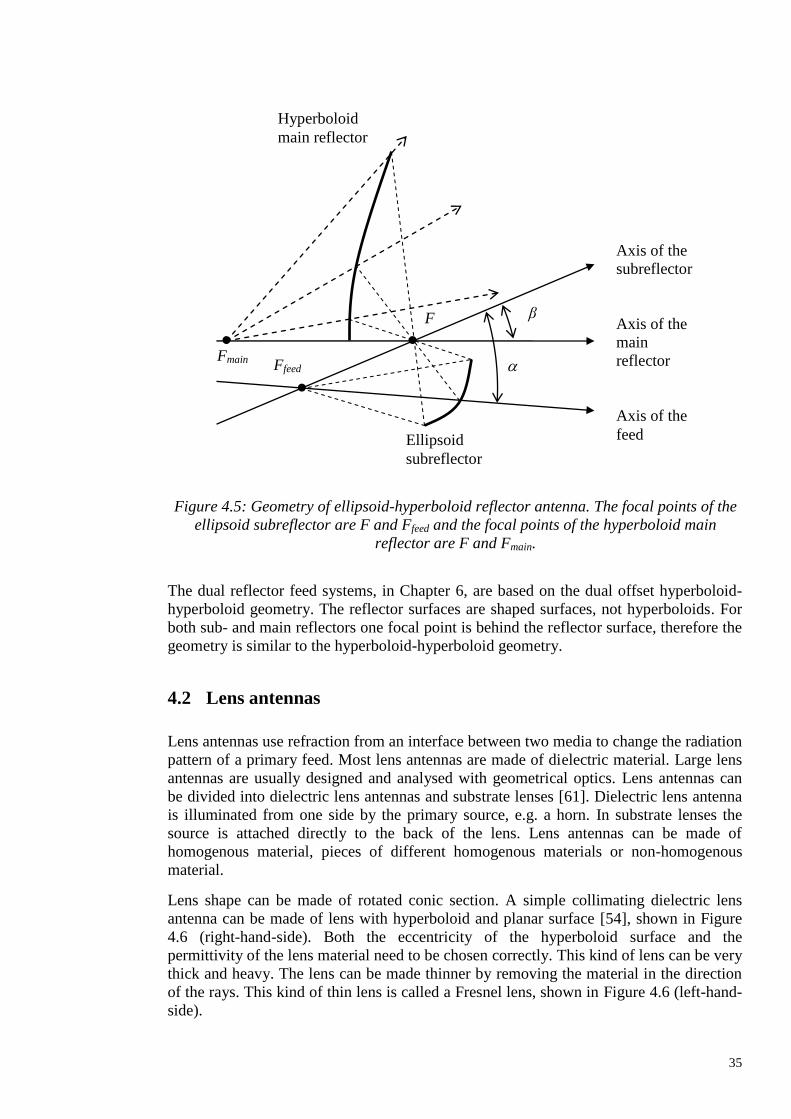
and the axis of feed [38]. As an example, ellipsoid-hyperboloid geometry is illustrated in
Figure 4.5.
Paraboloidal
main reflector
β
Elliptic subreflector
Ffeed
F
Axis of the
subreflector
Axis of the
main
reflector
Axis of the
feed
Figure 4.4: Geometry of a Gregorian type offset reflector antenna. The focal point
of the main reflector is F and the focal points of the subreflector are F and Ffeed.
Page 35
35
The dual reflector feed systems, in Chapter 6, are based on the dual offset hyperboloid-
hyperboloid geometry. The reflector surfaces are shaped surfaces, not hyperboloids. For
both sub- and main reflectors one focal point is behind the reflector surface, therefore the
geometry is similar to the hyperboloid-hyperboloid geometry.
4.2 Lens antennas
Lens antennas use refraction from an interface between two media to change the radiation
pattern of a primary feed. Most lens antennas are made of dielectric material. Large lens
antennas are usually designed and analysed with geometrical optics. Lens antennas can
be divided into dielectric lens antennas and substrate lenses [61]. Dielectric lens antenna
is illuminated from one side by the primary source, e.g. a horn. In substrate lenses the
source is attached directly to the back of the lens. Lens antennas can be made of
homogenous material, pieces of different homogenous materials or non-homogenous
material.
Lens shape can be made of rotated conic section. A simple collimating dielectric lens
antenna can be made of lens with hyperboloid and planar surface [54], shown in Figure
4.6 (right-hand-side). Both the eccentricity of the hyperboloid surface and the
permittivity of the lens material need to be chosen correctly. This kind of lens can be very
thick and heavy. The lens can be made thinner by removing the material in the direction
of the rays. This kind of thin lens is called a Fresnel lens, shown in Figure 4.6 (left-hand-
side).
Hyperboloid
main reflector
β
Ellipsoid
subreflector
Ffeed
F
Axis of the
subreflector
Axis of the
main
reflector
Axis of the
feed
Fmain
Figure 4.5: Geometry of ellipsoid-hyperboloid reflector antenna. The focal points of the
ellipsoid subreflector are F and Ffeed and the focal points of the hyperboloid main
reflector are F and Fmain.
Page 36
36
Figure 4.6: Examples of dielectric lens antennas; 1) Fresnel, and 2) hyperboloid.
Substrate lens made of an ellipsoid fed from a focal point is a collimating antenna. The
eccentricity has to be equal to 1/n, where n is the refractive index of the lens material
[62]. The elliptical lens can be approximated with a simple extended hemispherical lens
[62]. The synthesised ellipsoid with an extended hemispherical lens and a true ellipsoid
lens shape examples are illustrated in Figure 4.7.
Figure 4.7: An example of a substrate lens: synthesised ellipsoid with an extended
hemispherical lens [62].
Classical example of a non-homogenous lens antenna is a Luneburg lens [63], [64]. An
ideal Luneburg lens is a sphere with a varying relative permittivity that follows the
following equation: [63]
2
2
R
rrr , (4.4)
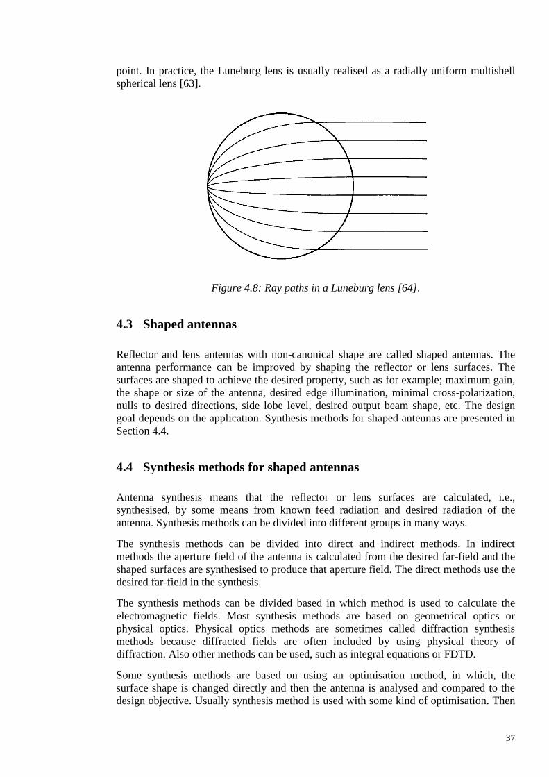
where r is distance from the centre and R is the radius of the lens. The ray paths inside a
Luneburg lens are illustrated in Figure 4.8. The lens collimates all rays from the focal
Page 37
37
point. In practice, the Luneburg lens is usually realised as a radially uniform multishell
spherical lens [63].
Figure 4.8: Ray paths in a Luneburg lens [64].
4.3 Shaped antennas
Reflector and lens antennas with non-canonical shape are called shaped antennas. The
antenna performance can be improved by shaping the reflector or lens surfaces. The
surfaces are shaped to achieve the desired property, such as for example; maximum gain,
the shape or size of the antenna, desired edge illumination, minimal cross-polarization,
nulls to desired directions, side lobe level, desired output beam shape, etc. The design
goal depends on the application. Synthesis methods for shaped antennas are presented in
Section 4.4.
4.4 Synthesis methods for shaped antennas
Antenna synthesis means that the reflector or lens surfaces are calculated, i.e.,
synthesised, by some means from known feed radiation and desired radiation of the
antenna. Synthesis methods can be divided into different groups in many ways.
The synthesis methods can be divided into direct and indirect methods. In indirect
methods the aperture field of the antenna is calculated from the desired far-field and the
shaped surfaces are synthesised to produce that aperture field. The direct methods use the
desired far-field in the synthesis.
The synthesis methods can be divided based in which method is used to calculate the
electromagnetic fields. Most synthesis methods are based on geometrical optics or
physical optics. Physical optics methods are sometimes called diffraction synthesis
methods because diffracted fields are often included by using physical theory of
diffraction. Also other methods can be used, such as integral equations or FDTD.
Some synthesis methods are based on using an optimisation method, in which, the
surface shape is changed directly and then the antenna is analysed and compared to the
design objective. Usually synthesis method is used with some kind of optimisation. Then
Page 38
38
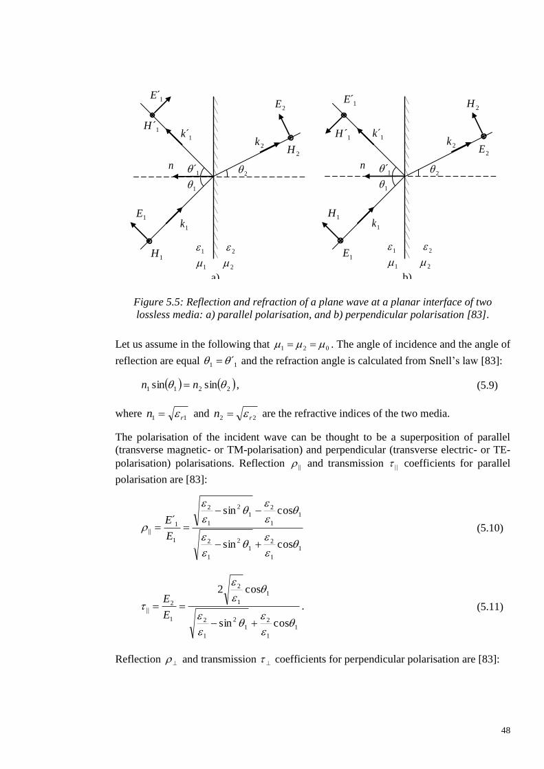
the synthesis objective (or basic geometry etc.) is changed, the shaped surfaces
synthesised, and then the antenna is analysed and compared to the design objective.
Synthesis methods are usually developed for a specific antenna type. Synthesis method
can be divided for reflector synthesis methods and lens synthesis methods. Some
synthesis methods can be used for both reflector and lens antennas.
The synthesis method used to design feed systems for hologram-based CATR is
numerical geometrical optics based direct synthesis method that is used together with an
iterative optimisation. This synthesis method is explained in detail in Chapter 5.
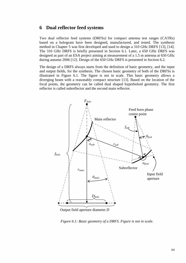
In Sections 4.4.1 and 4.4.2, some examples of reflector synthesis methods are presented.
Examples of lens synthesis methods are presented in Sections 4.4.3 and 4.4.4.
4.4.1 Reflector synthesis methods
A GO-based indirect synthesis method is presented in [65]. The shaped dual reflector
surfaces are determined by solving a pair of first-order ordinary nonlinear differential
equations. Example of dual-reflector system which will produce a uniform phase and
amplitude distribution in the aperture of reflector is given.
A GO-based indirect synthesis method based on solving a nonlinear second-order partial
differential equation of the Monge-Ampère type is presented in [66]. The method is used
for offset dual reflectors. A similar method is presented in [67].
An example of direct PO-based synthesis is in [68]. The reflector surfaces are
characterized with polynomials and Fourier series and optimised based on PO
simulations in comparison to desired gain pattern.
An indirect PO-based method is described in [69]. In this method, GO using Monge-
Ampère approach is used as a starting point for the final PO optimisation. A numerical
example of a contour-beam shaped reflector antenna is given.
A generalized diffraction synthesis technique is described in [70], where the synthesis
method combines optimisation procedures, physical optics and diffraction analysis with
the physical theory of diffraction. The shaped reflectors are represented by a set of
orthogonal global expansion functions and optimised with a safeguarded Newton's
method. The synthesis is generalized for single- and dual-reflector antennas fed by either
a single feed or an array feed.
A direct PO-based method using the successive projections method is presented in [71].
As an example, the technique is used to design a satellite antenna providing shaped beam
for a regional coverage area.
4.4.2 Ray-tracing based reflector synthesis methods
An indirect ray-tracing based synthesis method is presented in [72]. It is formulated for a
shaped dual offset reflector antenna based on a basic geometry of either a Cassegrain or a
Gregorian system. Rotational symmetry is assumed for feed pattern and for the desired
aperture field pattern. First-order approximation is used for the surfaces.
Page 39
39
Reflector surfaces and wave-fronts are described in terms of curvature parameters of the
bi-parabolic expansions in [73]. It is an indirect ray-tracing based synthesis method for
dual offset reflector antennas. To get the aperture mapping exact extra variables are
added to the mapping, i.e., by allowing the radial lines of the aperture ray grid to be
curved. Using the bi-parabolic expansions for surfaces and wave-fronts makes the
solution easier to control [73]. The synthesis technique has been used for shaped offset
dual reflectors antennas and for a dual reflector feed for a spherical reflector.
In [35], an indirect ray-tracing based synthesis method, with first-order approximation for
the surfaces, is presented. The method is used to design a dual reflector feed system
(DRFS) for a single reflector CATR. The system is described as a tri-reflector system
with two shaped reflectors of the DRFS and the parabolic reflector of the original CATR.
Another indirect ray-tracing based synthesis method, with first-order approximation for
the surfaces, is presented in [74].
4.4.3 Substrate lens synthesis methods
A direct GO-based method for axis-symmetric substrate lens is presented in [75]. GO is
used to obtain a first guess of the lens shape and PO formulation is used to compute the
actual far-field radiation pattern. In [76], this method is used for a 3D shaped lens that is
interpolated from two profiles that are calculated independently for two planes of the
lens. In [77], the method is generalised also for a shaped double-shell dielectric lens
antenna.
A direct GO-based method for 3D substrate lenses of arbitrary shape is presented in [78].
Second-order partial-differential equation derived from GO principles is solved with
iterative algorithm. Then, a local surface optimisation of the lens profile a multi-
dimension conjugate-gradient method is carried out to finally optimise the lens profile.
4.4.4 Dielectric lens synthesis methods
Indirect GO-based dielectric lens synthesis method is presented in [79]. The profiles of
rotationally symmetric lens surfaces are calculated numerically from a non-linear
differential equation.
Indirect ray-tracing based dielectric lens synthesis method is presented in [43]. A first-
order approximation is used for the surfaces of the rotationally symmetric lens. Also,
coma correction zoning is used to correct the cubic phase errors associated with the
shaped lens for off-axis beams [43].
In [80], an asymmetric lens is designed by optimising polynomial describing the second
surface of the lens, while the first surface collimates the beam. The shaped surface is used
to produce a shaped phase distribution to the aperture. GO and two dimensional
integration of the aperture distribution is used to calculate radiation patterns.
In [81], a multi-beam lens antenna is designed by optimising the coordinates of the lens
shape and the feed positions with a genetic algorithm (GA). The radiation patterns are
calculated with ray-racing and aperture integration. The GA optimisation is done based
on both high gain and low side-lobe level requirements.
Page 40
40
4.5 Feed systems for hologram-based CATR
Feed system for a hologram-based CATR is used to provide the desired modified
illumination for the hologram. The advantages of using a modified illumination are
discussed in Section 2.3.3.2. Desired modified illumination has a spherical wave, low
cross-polarisation, and amplitude pattern with flat amplitude to the centre of the
hologram and edge tapering to the hologram edge. The desired main polarisation
amplitude distribution is illustrated in Figure 4.9.
Figure 4.9: Desired hologram illumination; rotationally symmetric Butterworth-type
amplitude pattern.
A feed system with two shaped surfaces is used to modify both the amplitude and phase
patterns of a primary feed. A feed system for a hologram-based CATR is either a dual
reflector feed system (DRFS), explained in Chapter 6, or a shaped lens feed system,
explained in Chapter 7. In practice, the first shaped surface modifies the amplitude
pattern and the second corrects the phase pattern.
A corrugated horn is a good choice for a primary feed because corrugated horn typically
has a symmetrical beam and low cross-polarisation. A corrugated feed horn has been
used as the feed in all the designed feed systems for hologram-based CATR. Amplitude
and phase patterns of a 650 GHz feed horn are shown in Figure 4.10.
Page 41
41
Figure 4.10: Feed horn radiation pattern; amplitude and phase of the horizontal, vertical
and diagonal cuts at the vertical polarisation.
The feed system modifies the feed radiation pattern in Figure 4.10 into the hologram
illumination in Figure 4.9. In general, the hologram is not in the far-field of the feed
system, therefore the far-field pattern of the feed system is not of interest. The feed
system is designed to provide the illumination for the hologram area to a given distance,
i.e., to a circular area with the hologram diameter Dholo at distance of the hologram focal
length fholo. In practice, a feed system can be used for any hologram if the ratio fholo/Dholo
remains the same.
A hologram, designed for a modified illumination, is used only to transform the spherical
wave to a plane wave. Therefore, the amplitude pattern of the illumination, i.e., the width
of the area with the flat amplitude, determines the QZ size. The beam width of the feed
system needs to be as wide as possible. Amplitude tapering is needed to the edge of the
hologram to avoid strong diffraction from the hologram edges. The combination of a
wide beam and amplitude tapering to the edge is difficult to realise and a compromise has
to be made.
Page 42
42
5 Numerical synthesis method
Numerical synthesis method for designing a feed system for a hologram-based CATR is
described in this chapter. The synthesis method was developed specifically for designing
a dual reflector feed system (DRFS) for a hologram-based compact antenna test range
(CATR) [14], [13]. In this thesis the method is generalised also for lens antenna feed
systems. Both reflector and lens feed systems are based on modifying the field radiated
by the primary feed with two shaped surfaces.
The synthesis method is a direct ray-tracing-based synthesis procedure, that is based on
the method described in [73] with some simplifications. In the synthesis the
electromagnetic fields are represented with rays that represent the local plane wave
amplitude and phase. The surfaces are approximated with locally planar sections. The
synthesis of the feed system starts with defining the basic geometry. Then input and
output fields and rays are defined. Finally, the reflector (or lens) surfaces are synthesised
and the edges are rounded.
This synthesis method was developed because existing synthesis methods were not
directly applicable [13]. For example, methods in [35] and [74] are based on similar ray-
tracing principles, but are developed for different antenna type. This results in a
somewhat different approach in the synthesis [13]. Also, the optimisation procedure, as
explained in Section 5.2, is an important part of the developed synthesis method.
The basic properties of rays and ray-tracing are explained in Section 5.1 in homogenous,
isotropic, lossless medium using the local plane wave approximation for the wave fronts.
Section 5.1 provides the ray properties that are used in the synthesis of shaped surfaces in
Section 5.3 and in ray-tracing simulation in Section 5.4.2.
The design procedure, explained in Section 5.2, is an iterative process in which the
shaped antenna structure is synthesised (Section 5.3), simulated (Section 5.4) and the
simulation results analysed. The antenna parameters are optimised based on the
simulation results.
Two dual reflector feed systems have been designed using this synthesis method, one for
310 GHz [14], [13] and one for 650 GHz [16], [17]. These feed systems are presented in
Chapter 6. Design of the 650 GHz DRFS is presented in more detail in Section 6.2. A
lens antenna feed system is presented in Chapter 7 to demonstrate that the synthesis
method is usable also for lens antennas.
5.1 Properties of rays and ray-tracing
Properties of geometrical optics fields and rays are described in this section in
homogenous, isotropic, lossless medium using a local plane wave approximation for the
wave fronts. These ray properties are derived from the theory of geometrical optics
introduced in Section 3.4. With these approximations the geometrical optics equations are
greatly simplified. In ray-tracing, a geometrical optics field is represented with a discrete
number of rays, the path of each ray is calculated, and then the field is calculated from
the known rays.
Page 43
43
The purpose of this section is to provide a detailed list of ray properties with the
approximations listed above. First rays and ray tubes are defined and then their properties
and relation to fields are explained in the following sub-sections. Some of the ray
properties, described in this section, are not used in the synthesis of feed systems. Most
importantly polarisation properties are not taken into account in the synthesis.
5.1.1 Ray, ray tube, and field
A ray is a local representation of the electro-magnetic field. A ray represents a plane
wave. Ray properties are the starting point, end point, direction, length, properties of the
medium, and complex electric field vector (field amplitude, phase, and polarisation).
Field phase changes along the ray, therefore, it has to be defined at least at some point
along the ray. The ray amplitude is not (necessarily) the same as the field amplitude
(Section 5.1.7).
A ray tube is a volume between rays (see example in Figure 5.4).
A field is a complex valued vector field E . A field is defined as continuous function or in
discrete points. A field has amplitude, phase and polarisation.
5.1.2 Ray direction
In general, a ray path is solved from Equation (3.29) (ray equation). For homogenous
medium n(r) = n, a ray can be described simply as
rsr 0 , (5.1)
where s is distance along a ray and r is the ray direction and 0r is the starting point of
the ray. A ray in a homogenous medium is a straight line. The ray represents the direction
of propagation, which is the same as that of the local wave vector )(rk .
5.1.3 First-order wave front approximation
A wave front is a surface where the field phase is constant. A wave front is normal to a
ray direction. In GO, the wave front is approximated locally for each ray. Often the wave
front is approximated with a second-order approximation that is characterised with two
principal radii and directions of curvature [54], [55], [73]. A wave front can also be
approximated with a plane-wave, i.e., a first-order approximation [13], [16]. The second-
and first-order approximations are illustrated in Figure 5.1.
Page 44
44
Figure 5.1: Local approximation of a wave front; a) second-order and b) first-order
approximation [13].
The most important difference between these approximations is that with the second-
order approximation amplitude changes along a ray, which is described with the wave
front curvature parameters. With the first-order approximation the ray amplitude does not
change along the ray and the changing field amplitude is represented (or calculated) using
ray tubes as explained in Section 5.1.7.
5.1.4 Amplitude, phase, and polarisation along a ray
One ray represents a plane wave in a homogenous, isotropic, lossless medium. The ray
amplitude E or polarisation does not change along the ray. Phase decreases along the
ray linearly in the direction of propagation (ray direction), so that distance of one
wavelength corresponds to a phase change of -360. The phase depends on a distance
s along a ray as:
sskss rr
0
22 . (5.2)
With one ray (or parallel rays), if the field is known at a point s0 along the ray, the field at
point s along the ray is:
)(
00)()(
ssjkesEsE
. (5.3)
The field phase is a relative quantity defined in relation to a phase reference; therefore
also the ray length calculated from the field phase is a relative quantity.
Page 45
45
5.1.5 Ray direction and known focal point
Ray directions can be determined from a known far-field pattern that is defined as an
angular field distribution originating from a focal point. All rays originate from the focal
point. The field phase affects the ray length, not the ray direction.
5.1.6 Ray direction and field phase
The ray direction can be determined from a known field phase. The phase derivatives
determine tangential vectors of a plane, i.e., the constant phase wave front of a plane
wave. The wave front plane is determined from the phase derivatives using the relation of
the phase and ray length in (5.2). The ray direction is normal to the wave front plane.
For example, let’s consider a rotationally symmetric geometry in Figure 5.2. The field
phase is known on z = 0 plane and the phase pattern is rotationally symmetric, i.e.,
0/ . The field source is known to be somewhere above the z = 0 plane. The ray
direction angle , angle relative to the z-axis, is [82]:
k
1sin . (5.4)
Similarly, if the field is known at discrete points, the ray direction can be calculated from
the geometry shown in Figure 5.3, where s is calculated from the phase difference:
z
θ
/
Figure 5.2: Determining ray direction from field phase; a rotationally
symmetric geometry.
Page 46
46
nns 12
. (5.5)
5.1.7 Power, amplitude and ray tubes
Power stays inside a volume bounded by rays, i.e., inside a ray tube. Power density varies
as a function of cross-sectional area of the ray tube. Power that propagates in a ray tube
that has cross-sectional surface S is calculated from the real part of Poynting’s vector
SS
dSnrEdSHEP2
2
1Re
2
1
, (5.6)
where E is the electric field on the surface S, r is ray direction unit vector and n is
normal unit vector of the surface S.
Lets examine a simple ray tube between three rays 1r , 2r , and 3r with electric fields 1E ,
2E , and 3E , respectively. The ray tube and its planar cross-section are shown in Figure
5.4. In general, a ray tube can be defined between anything from three to an infinite
number of rays and the cross-section does not have to be a plane. Three rays and planar
cross-section is the simplest example without making assumptions on the ray directions.
s
n
1 n
r
θ
Figure 5.3: Determination of ray direction from known field phase in
case of nn 1 .
Page 47
47
The power going through surface S in Figure 5.4 cannot be calculated exactly because the
electric field and ray directions are known only on the discrete points where the rays
intersect the surface. Integral in (5.6) can be approximated for example with an average
nrEnrEnrEA
dSnrEPS
3
2
32
2
21
2
1
2
32
1
2
1
. (5.7)
Sometimes it can be approximated that 1 nr . This approximation is accurate if the ray
direction r is parallel to the normal vector n of the cross-sectional surface, i.e., if the
rays are parallel (or almost parallel) to each other and to the normal n . In this case the
tube power is simply
AEP ave
2
2
1
, (5.8)
where 2
aveE is the average of squared amplitudes of the rays that define the tube.
5.1.8 Reflection and refraction from a planar surface
When a ray (a plane-wave) encounters a boundary between two different media it is
reflected and refracted from the boundary, as illustrated in Figure 5.5. The incident wave
comes at an angle 1 compared to the normal n . Part of the incident wave is reflected at
an angle 1´ and a part is refracted (transmitted) into medium 2 at an angle 2 . The
tangential components of the wave vectors are identical.
1r
2r
3r
n
1E
3E
2E
S
Figure 5.4: Example of a ray tube and its planar cross-section.
Page 48
48
Let us assume in the following that 021 . The angle of incidence and the angle of
reflection are equal 11 ´ and the refraction angle is calculated from Snell’s law [83]:
2211 sinsin nn , (5.9)
where 11 rn and 22 rn are the refractive indices of the two media.
The polarisation of the incident wave can be thought to be a superposition of parallel
(transverse magnetic- or TM-polarisation) and perpendicular (transverse electric- or TE-
polarisation) polarisations. Reflection | | and transmission | | coefficients for parallel
polarisation are [83]:
1
1
21
2
1
2
1
1
21
2
1
2
1
1||
cossin
cossin´
E
E (5.10)
1
1
21
2
1
2
1
1
2
1
2||
cossin
cos2
E
E. (5.11)
Reflection and transmission coefficients for perpendicular polarisation are [83]:
n 1́
1
1´k
1k
2k
2
1H
1E
1´H
1́E
2H
2E
n 1́
1
1´k
1k
2k
2
1E
1H
1´H
1́E
2E
2H
1 2
1 2
a)
1 2
1 2
b)
Figure 5.5: Reflection and refraction of a plane wave at a planar interface of two
lossless media: a) parallel polarisation, and b) perpendicular polarisation [83].
Page 49
49
11
2
1
2
1
2
1
21
1
1
cossin
sincos´
E
E (5.12)
11
2
1
2
1
1
2||
cossin
cos2
E
E.
(5.13)
In (5.10) – (5.13), 1E , 1́E , and 2E are the ray amplitudes of the incident, reflected, and
refracted rays, respectively.
Ray directions can be calculated from Snell’s law and the geometry in Figure 5.5. Other
possibility is to calculate the wave vectors 1k , 1´k , and 2k , as the ray direction is the
same as the wave vector direction. The tangential components of these wave vectors are
identical and the wave-numbers 11 ´kk and 2k are known:
If 21 , a total reflection occurs if [83]:
1
21
1 sin
. (5.14)
In case of a total reflection, reflection coefficients become complex numbers and 1||
and 1 , i.e., all of the incoming power is reflected. Reflection coefficients are
calculated from (5.10) and (5.12) and they affect only the phase of the reflected ray. The
ray amplitude of the refracted ray is set to zero 02 E .
In general, metal can be considered to be perfect electric conductor (PEC). Reflection
coefficient from metal surface for all polarisations and for all incident angles is ρ = –1.
5.1.9 Polarisation of reflected and refracted rays
The electric field vectors of the reflected and refracted (transmitted) rays are calculated
first by dividing the incident field 1E to the parallel ||
1||
1 uE and perpendicular 11 uE
components.
11
||
1||
11 uEuEE , (5.15)
where the amplitudes and directional unit vectors are:
Page 50
50
111 uEE ,
||
11||
1 uEE , (5.16)
1
11
kn
knu
,
11
11||
1
uk
uku . (5.17)
The reflected field is:
11
||
1||
1||1 ´´´ uEuEE , (5.18)
where directional unit vectors of reflected perpendicular and parallel polarisations are:
1
11
´
´´
kn
knu
, 11
11
11
11||
1
´´
´´
´´
´´´
ku
ku
uk
uku
. (5.19)
The refracted (transmitted) field is:
21
||
2||
1||2 uEuEE , (5.20)
where directional unit vectors of refracted perpendicular and parallel polarisations are:
2
22
kn
knu
,
22
22||
2
uk
uku . (5.21)
In (3.17), (3.19), and (3.21) 1k , 1́k , and 2k are the wave vectors, i.e., ray directions, and
n is the surface normal. Field vector, wave vector, and surface normal directions are
illustrated in Figure 5.5.
5.2 Feed system design procedure
The iterative design process used to design the feed systems for hologram-based CATRs
is shown in Figure 5.6. One iteration round of the design process has three parts: the
synthesis of the surfaces, simulations and analysis of the results. The synthesis of a feed
system can be divided into three parts: definition of the basic geometry, definition of
input and output fields and their representation with rays and the synthesis of the reflector
surfaces.
The simulation method depends on the antenna type. The dual reflector feed systems
have been simulated with a commercial reflector antenna simulation software GRASP8W
[84]. The lens antenna feed systems are simulated with a ray-tracing based simulation
method, described in Section 5.4.2. Finally the simulation results are analysed, i.e., the
amplitude and the phase are calculated from the simulation results, and compared to
previous simulation results.
Page 51
51
The design process is an iterative optimisation process. In general, first 1) the parameters
of the basic geometry are optimised, then 2) the input and output fields and their
representation with rays are optimised, and finally 3) the parameters of the synthesis are
optimised. Each of those three steps are discussed separately in detail in Sections 5.3.1 –
5.3.3. In practice the design process is not that straightforward because all of the steps in
the design process affect each other.
Each parameter is optimised by synthesizing the surfaces with a number of different
values for the parameter. Then the synthesised surfaces are simulated and the results
analysed. The best value for the parameter, based on the simulation results, is used when
the next parameters are optimised. In this way it is possible to study separately how each
parameter affects the radiation of the antenna.
It is most important to find the electrical and geometrical parameters that can and must be
optimised. After that it is fairly straightforward (but not easy) to parameterise and to find
the optimal parameter values.
5.3 Synthesis of a feed system
The reflector (lens) surfaces are synthesised from known input and output rays and the
geometry of the feed system by tracing the rays, using the Snell’s law for reflections
(refractions) and ray length adjustment. The synthesis has three steps: 1) defining the
basic geometry, 2) representation of fields with rays, and 3) the synthesis of the surfaces.
Known information in the beginning of synthesis of the surfaces, in case of a dual
reflector feed system, is illustrated in Figure 5.7.
Synthesis method
Synthesised antenna
Simulation
Simulation results
Analysis of the simulation results
Figure 5.6: Design process.
Page 52
52
The centre ray is known from the basic geometry. The centre ray interception points on
the surfaces are the first known points of the surfaces. The origins and the end points of
the input and output rays are determined from the focal points (from the geometry) and
from the input and output fields.
5.3.1 Basic geometry
The basic geometry definition includes:
1. Two focal points: feed horn phase centre point and focal point of the feed system.
The focal point of the feed system is usually the same as the hologram focal point
Fholo.
2. Centre ray path from the feed horn phase centre point to the centre of the output
field aperture, i.e., the hologram. The centre ray defines the first points of the
surfaces.
3. Input and output field aperture planes and diameters. Input and output fields are
defined in the aperture planes.
4. Coordinate systems; global coordinate system, feed horn coordinate system, input
and output aperture plane coordinates.
The definition of the basic geometry is mostly responsible for the size of the reflectors (or
lenses) and for the distances between feed horn, reflectors (lenses), and the hologram.
Output rays
Input rays
Feed horn phase centre point
F
Fholo
Output field aperture
Centre ray
interception
point (on
the main
reflector)
Input
field
aperture
Centre ray
interception
point (on the
subreflector)
Centre ray
Figure 5.7: Known information in the beginning of synthesis of the surfaces.
Page 53
53
The final shape and size of the reflectors (or lenses) are defined only after the synthesis of
the shaped surfaces.
5.3.2 Representation of fields with rays
The electromagnetic fields are represented with rays. A ray represents a plane wave
perpendicular to the ray direction.
The ray grid is defined in polar coordinates in the input and output aperture planes, as
illustrated in Figure 5.8. The ray grid is MN matrix with N rings and M rays on each
ring. The first ring is formed by M rays in the centre of the grid and the rays at = 0º are
duplicated at = 360º to facilitate the calculations. Flux tubes are formed by four
adjacent rays. The flux tubes are numbered so that tube (ntube, mtube) is cornered by rays
(nray, mray), (nray, mray+1), (nray+1, mray), and (nray+1, mray+1).
Ray grid in Figure 5.8 is a constant angular and radial polar grid, i.e., a grid with constant
∆ and constant ∆ρ. Sometimes a grid with varying ∆ρ is used.
5.3.2.1 Input field
The input ray amplitudes are interpolated from the vertical polarisation, i.e., main
polarisation, of the radiation pattern of the feed horn. The input rays are defined so that
they originate from the feed horn phase centre point and intersect the input field aperture
plane at points defined by the input ray grid at MN discrete points. The feed horn phase
centre point and the input field aperture plane are illustrated in Figure 5.7. The phase of
the feed horn main polarisation can be taken into account in ray length adjustment in the
synthesis of the surfaces. Often the feed horn phase pattern has very small effect and it
can be neglected in the synthesis.
∆
∆ρ
1 and M
M-1
M-2
2
3
2 3 4 N
Flux tube (3,2)
Ray (3,2)
Figure 5.8: Ray grid and flux tubes.
Page 54
54
5.3.2.2 Output field
The output field is defined in the output field aperture plane at constant angular and
constant radial polar grid at MN discrete points. Finally the output ray grid is
determined in the aperture mapping. The output rays originate from the hologram focal
point Fholo and end in the output field aperture plane, as shown in Figure 5.7. The desired
output field (main polarisation) amplitude and phase are defined by the user.
The feed system is used to generate a spherical wave-front with flat amplitude in the
centre of the beam and amplitude tapering towards the edge of the hologram. This can be
achieved for example using a rotationally symmetric Butterworth-type function for the
output field amplitude:
N
c
E2)/'(1
1)'(
, (5.22)
where ρc and N are the –3 dB point and the degree of the Butterworth function and ρ’ is
the output field aperture coordinate. The output field phase is modified by adjusting the
total lengths of the rays in the synthesis of the surfaces.
5.3.2.3 Aperture mapping
The input rays are mapped to the output rays, i.e., the output ray grid is changed so that
the power in each ray tube is the same in the output as in the corresponding input ray
tube.
The mapping is done in two parts, first the amplitudes of the output rays are scaled to
make the total output power equal to the total input power and then the new output field
aperture coordinates are calculated so that the power is equal for each ray tube, i.e.,
),(),( tubetubeouttubetubein mnPmnP . (5.23)
The input ray amplitudes and the output ray amplitudes have been normalised so that the
peak values are set to one. The normalised output ray amplitudes Eout,norm are scaled so
that the total power of the output flux tubes is equal to the total power of the input flux
tubes. The scaling factor α is
1
1
1
1
,
1
1
1
1
),(
),(
M
m
N
n
tubetubenormout
M
m
N
n
tubetubein
tube tube
tube tube
mnP
mnP
. (5.24)
The tube powers ),( tubetubein mnP and ),(, tubetubenormout mnP are calculated from (5.6) or (5.8).
The new output field aperture coordinates, i.e., the output ray grid, are calculated from
the integral expressions of (5.23) using scaled output ray amplitudes:
Page 55
55
rayraynormoutrayrayout mnEmnE ,, , . (5.25)
Aperture mapping does not take into account reflection (or transmission) coefficients or
depolarisation (
outin uu , ||||
outin uu ).
5.3.2.4 Rotationally symmetric aperture mapping
Aperture mapping is greatly simplified if the fields are assumed to be rotationally
symmetric. The ray grids are defined by N ray rings. The output field amplitude is
defined as a rotationally symmetric function Eout,norm(nray) and the input field is averaged
1
),(
)(
1
1
M
nmE
nE
M
m
rayrayin
rayin
ray.
(5.26)
The output ray amplitudes are scaled
raynormoutrayout nEnE , , (5.27)
where the scaling factor is
1
1
,
1
1
)(
)(
N
n
tubenormout
N
n
tubein
tube
tube
nP
nP
. (5.28)
The ray ring power, with the approximation of 1 nr , in (5.8) becomes:
22
1
22
2
2
)()1(
2
1
2
1)( nn
rayinrayin
avetubein
nEnEAEnP
, (5.29)
where n and 1n are the input ray ring coordinates at the input aperture for ray rings
nray and nray+1, respectively. The total power in each ray ring is known from (5.29). The
new output field aperture coordinates are calculated so that the power is equal for each
ray ring, i.e.,
)()( tubeouttubein nPnP . (5.30)
The output field Eout(nray) is known in a constant ∆ ' grid (or some other user defined
grid). The power density is approximated to be a linear function between the known
points, i.e., when ' n ≤ ' ≤ ' n+1
)(')()'(2
tubetubeout nbnkE , (5.31)
where )( tubenk and )( tubenb are calculated from Eout(nray) and Eout(nray+1)
Page 56
56
nn
rayoutrayout
tube
nEnEnk
''
1)(
1
22
(5.32)
rayouttube nEnb 2)( . (5.33)
The new output aperture coordinates ρ’ are calculated, starting from the centre of output
field aperture, by solving ρ’n+1 from
1'
'
2 ''2)'(2
1)()(
n
n
dEnPnP outtubeouttubein
, (5.34)
where )'(2 outE is a piece-wise continuous function calculated using (5.31).
The incident angles of the rays to the aperture planes, i.e., nr , could be taken into
account in the mapping by replacing 2E with nrE 2 in (5.28)–(5.34).
5.3.3 Synthesis of the surfaces
The shaped surfaces are synthesised from the known input and output rays and from the
geometry of the feed system by tracing the rays, using Snell’s law for reflections (or
refraction) and ray length adjustment. The surfaces are assumed locally planar. The
synthesis procedure is similar for both dual reflector and lens feed systems as both have
two shaped surfaces. The synthesis is explained for a general offset geometry. Rotational
symmetry in case of lens feed systems in Chapter 7 simplifies the synthesis as only one
radial cut is necessary to synthesise.
The known information in the beginning of the synthesis is illustrated in Figure 5.7. The
centre ray is known from the basic geometry. The centre ray interception points on the
surfaces are the first known points. Synthesis starts from the centre ray and progresses
ring by ring in counter-clock wise direction to the aperture rim. After the centre ray the
synthesis procedure is the same for each ray. The synthesis procedure is described in
Figure 5.9.
The 1st shaped surface is directly illuminated by the feed horn and it is mainly responsible
for modifying the amplitude. The 2nd
shaped surface is used to correct the phase.
Page 57
57
First the tangential planes at the centre ray interception points are calculated using Snell’s
law
ir
ir
rr
rrn
, (5.35)
where n is the surface normal vector, ir is the directional vector of the incident ray and
rr is the directional vector of the reflected ray.
After the centre ray the synthesis procedure is the same for each ray. For a ray (nray, mray)
the input and output rays, the anterior points (nray–1, mray) and the horizontal and vertical
tangents at the anterior points are known. Calculation of the next point of a surface is
illustrated in Figure 5.10.
Input and output rays, anterior points, tangents at
the anterior points
1st interception point
2nd
interception point with ray path length
adjustment
Tangential planes at interception points with
Snell’s law
Repeated
for all
rays
Figure 5.9: Synthesis procedure.
Page 58
58
The 1st surface point (nray, mray) is the interception point of the input ray (nray, mray) and
the tangential plane at the anterior point, i.e., at the point (nray–1, mray).
The 2nd
surface point (nray, mray) is calculated in a similar way as the interception point of
the output ray (nray, mray) and the tangential plane at the anterior point, i.e., point (nray–1,
mray) of the 2nd
surface. The 2nd
surface point is then moved along the output ray to adjust
the total length of the ray l(nray, mray) from the feed horn phase centre point to the output
field aperture. The desired ray length is
),(2
),('),( 022
rayrayinholorayrayrayray mnfmnmnl
Cmn rayrayout ),(2
0
,
(5.36)
where fholo is the hologram focal length, in is the feed horn phase pattern, out is the
desired output field phase, and C is a constant. The desired ray length is known for the
centre ray from the geometry, therefore the constant C can be solved from (5.36) written
for the centre ray. In case of a shaped lens feed system the desired ray length is an
electrical ray length taking into account the electrical properties of the lens.
After the surface points are known, the horizontal and vertical tangents are calculated
from the input ray, the ray from the 1st surface point to the 2
nd surface point and the
output ray using the Snell’s law as explained in Section 5.1.8.
After the synthesis the shaped surfaces are fitted to planes with rounded sections. The
rounding is needed to reduce edge diffraction. Also, the planar sections around the
shaped surfaces facilitate the mechanical construction of the feed system.
antir , antrr ,
antn
antt
ir rr
n
t
antir ,
antn
antt
antrr ,
ir
n
t
rr
a) b)
Anterior point Next point
Figure 5.10: Calculation of the next point of the surface: a) reflection, b) refraction.
Page 59
59
5.4 Simulations
The design procedure, as explained in Section 5.2, is based on iterative optimisation of
the synthesis parameters based on simulation results. The simulation method depends on
the feed system type. The dual reflector feed systems are simulated with GRASP8W, as
described in Section 5.4.1. A ray-tracing method is used to simulate the shaped lens feed
systems. This ray-tracing method is described in Section 5.4.2.
5.4.1 Simulations with GRASP8W
GRASP8W is used to simulate the dual reflector feed systems [13], [16]. In GRASP8W
physical optics (PO) is used to calculate the field radiated by a reflector antenna. Physical
theory of diffraction (PTD) can be used to include diffracted fields from the reflector
edges.
Simulated feed horn radiation pattern and data of the feed system geometry and shape of
the reflectors are needed for the simulation. First, surface currents on the subreflector (1st
surface) are calculated from the feed horn radiation pattern. Then the surface currents on
the main reflector (2nd
surface) are integrated from the currents on the subreflector.
Finally the field illuminating the hologram is calculated from the current elements on the
main reflector. Amplitude, phase and cross-polarisation level can be calculated from the
field data given by the GRASP8W software.
5.4.2 Ray-tracing simulation
A ray-tracing method is used to simulate the shaped lens feed systems. The method is
based on calculating the aperture field by ray-tracing through the lens (or lenses). The
ray-tracing is based on the same principles and approximations as the synthesis in Section
5.3. The hologram illumination is integrated from the aperture field with Huygens’
principle. Ray definition and ray-tracing is explained in Section 5.4.2.1, aperture field
calculation in Section 5.4.2.2, and calculation of the hologram illumination in Section
5.4.2.3.
The shaped lens feed systems are rotationally symmetric and therefore also the ray-
tracing simulation is rotationally symmetric. The rotational symmetry means that it is
necessary to find the ray paths for only one radial cut. After the ray paths have been
found ray tube powers and transmission coefficients can be calculated for both vertical
and horizontal cuts. The two-dimensional hologram illumination field is integrated from
the two-dimensional aperture field, i.e., without the rotational symmetry assumption.
5.4.2.1 Ray definition and ray tracing to the aperture
Rays are set to originate from the feed horn focal point. Number of rays and the input
beam half-beam width θfeed are, in general, different than in the synthesis. The ray path is
calculated from the feed horn focal point to the aperture plane that is a plane
perpendicular to the symmetry axis immediately after the lens (or after lenses).
The geometry and the lens surfaces are known from the synthesis. The surfaces include
the shaped surfaces and the rounded edge regions. The shaped surfaces are defined by the
Page 60
60
interception points of input and output rays and the tangential planes of the anterior
points in the synthesis. In the simulation the surfaces are approximated with planar
sections between the known points from the synthesis.
Calculation of the ray path is identical for each surface of the lens (or lenses). The
geometry involved in calculating the refracted ray is illustrated in Figure 5.11. The
incident ray is known, it is either a ray originating from the feed horn focal point or a
refracted ray from a previous surface. First the interception point of the incoming ray and
the surface is calculated. The refraction angle θ2 is calculated from the incident angle θ1
and from the electrical properties (ε1 and ε2) using Snell’s law (5.9). The refracted ray can
be calculated from the refraction angle θ2.
An example of ray-tracing through two shaped lenses is shown in Figure 7.7 on page 85.
In Figure 7.7, the feed horn focal point is at z = 295 mm and the aperture plane at z = 0
mm.
The final result of the ray-tracing for each ray n = 1 ... N includes: ray end point at the
aperture n' , incident angles θ1 for each surface, and total electrical ray length nl totel, .
The θ1 angles are used to calculate the transmission coefficients. The electrical ray length
is
ll rel , (5.37)
i.e., the electrical ray length is r times longer than the geometrical ray length inside a
lens. Total electrical ray length is the sum of ray lengths from the feed horn focal point to
the aperture.
5.4.2.2 Calculation of the aperture field
The ray tube powers tubein nP are calculated using (5.29) as in the synthesis, except that
now the rays and input aperture plane are the ones used in the ray-tracing simulation. The
vertical polarisation, i.e., the main polarisation, of the radiation pattern of the feed horn is
used in the ray tube power calculations.
θ1
θ2 Refracted ray
Incident ray ε1
ε2
Figure 5.11: Calculation of refracted ray.
Page 61
61
In the aperture plane the ray tube ring ntube is between rays nray and nray+1, i.e., between
ray end points n' and 1' n . The aperture field amplitude is calculated from the ray tube
powers. Instead, the ray lengths and transmission coefficients are determined at the ray
end points. Therefore, the aperture field is first calculated at points
1''2
1' nntuben . (5.38)
Total electrical ray lengths are
12
1,,, raytotelraytoteltubetotel nlnlnl . (5.39)
Transmission coefficients are calculated with (5.11) and (5.13). The total transmission
coefficient at tuben' is
surf surfN
i
N
i
rayirayitube nnnT1 1
)1()(2
1 , (5.40)
where Nsurf is the number of surfaces, and )( rayi n is the transmission coefficient of ith
surface for ray nray.
The tube power at the aperture is
tubeintubetubea nPnTnP2
. (5.41)
The field amplitude at points tuben' is calculated from the tube powers at the aperture.
Using the expression for the tube power in (5.8) the tube power at the aperture is
tubeatubeatubea nAnEnP2
02
1
, (5.42)
where tubea nA is the ray ring area in the aperture:
22
1 '' nntubea nA . (5.43)
The field amplitude at points tuben' is
tubea
tubeintubetubein
tubea
tubeintubetubea
nA
nAnTnE
nA
nPnTnE
02
. (5.44)
The aperture field phase is calculated from the electrical ray lengths, therefore aperture
field is
tubetotel nljk
tubeatubea enEnE ,0 . (5.45)
The radiation pattern of the feed horn is different for vertical and horizontal cuts. Also,
the transmission coefficients depend on the polarisation. The vertical and horizontal cuts
Page 62
62
of the ray amplitudes in the aperture tubever nE and tubehor nE are calculated from
(5.45); tubever nE with | | (5.11) and vertical cut of inP , and tubehor nE with (5.13)
and horizontal cut of inP .
The final two-dimensional aperture field ',' aE is calculated at constant angular and
radial polar grid, i.e., a grid with constant ' and constant ' .
Bbb
AaauEbaE
b
aybaaa
,...3,2,1,'½'
,...3,2,1,'½',',',
. (5.46)
In (5.46), the aperture field points are defined so that '½'' max A and
'½2' B . max' defines the size of the aperture.
Vertical and horizontal cuts of baaE ',' , i.e., averE ' and ahorE ' , are
interpolated from tubever nE and tubehor nE . The aperture field between the field cuts is
interpolated as:
ahorbaverbbaa EEE ''cos''sin',' 22 . (5.47)
5.4.2.3 Calculation of hologram illumination with Huygens’ principle
The field at the hologram is calculated from the aperture field with Huygens’ principle as
explained in Section 3.1. Let’s first define the aperture field and the hologram
illumination field.
Aperture field is ymnaa uEmnE ',', from (5.46). The aperture field is defined at
azz ' , i.e., at the aperture plane. The polarisation of the aperture field is linear vertical
polarisation. The hologram illumination field is: (at 0z )
Lll
KkkuElkE
l
kylkhh
,...3,2,1,
,...3,2,1,,,,
. (5.48)
From (3.9), the vertical polarisation of the hologram illumination is:
B
b
A
a
h badAlkbaFlkE1 1
),(),,,(, , (5.49)
where
Page 63
63
ya
lkbajkR
a uzlkbaRlkbaR
jkebaElkbaF
32
,,,
,,,
1
,,,2
,),,,(
(5.50)
zablak uzuubarlkrlkbaR '',',,,, (5.51)
22'½''½'
2
'),(
aabadA . (5.52)
Equation (5.49) gives the hologram illumination accurately only if the number of aperture
field points is high enough. The required number of aperture field points can be tested by
increasing the number of points and testing the convergence of the resulting hologram
illumination.
In (5.49) the closed integral from (3.9) is replaced with a finite sum. This means that the
aperture field is assumed to be zero outside the area where the aperture field has been
calculated. In practice absorbers are used to limit the aperture size.
Page 64
64
6 Dual reflector feed systems
Two dual reflector feed systems (DRFSs) for compact antenna test ranges (CATRs)
based on a hologram have been designed, manufactured, and tested. The synthesis
method in Chapter 5 was first developed and used to design a 310 GHz DRFS [13], [14].
The 310 GHz DRFS is briefly presented in Section 6.1. Later, a 650 GHz DRFS was
designed as part of an ESA project aiming at measurement of a 1.5 m antenna at 650 GHz
during autumn 2006 [12]. Design of the 650 GHz DRFS is presented in Section 6.2.
The design of a DRFS always starts from the definition of basic geometry, and the input
and output fields, for the synthesis. The chosen basic geometry of both of the DRFSs is
illustrated in Figure 6.1. The figure is not in scale. This basic geometry allows a
diverging beam with a reasonably compact structure [13]. Based on the location of the
focal points, the geometry can be called dual shaped hyperboloid geometry. The first
reflector is called subreflector and the second main reflector.
Fholo
fsub
rmain
Output field aperture diameter D
Dholo
rsub αsub
Feed horn phase
centre point
Subreflector
Main reflector
fholo
Input field
aperture
αfeed
θfeed
θmain
Figure 6.1: Basic geometry of a DRFS. Figure is not in scale.
Page 65
65
The solid line in Figure 6.1 is the centre ray path. The feed horn location is defined by the
feed horn phase centre point. The feed angle is αfeed. The focal length of the subreflector
fsub is the distance between the feed horn phase centre point and the centre point of the
subreflector. The subreflector offset angle is αsub and the distance between the reflectors
is rsub. The focal point of the hologram is Fholo and that is also the focal point of the feed
system. The diameter of the hologram is Dholo. The focal length of the system is fholo and
the distance from main reflector to the hologram centre point is rmain.
For the synthesis of the shaped surfaces, the input and output fields are defined at the
aperture planes illustrated in Figure 6.1. Input field is defined at the input field aperture
from the far-field pattern of the feed horn. Input half-beam width, i.e., the feed half-beam
width, is θfeed. The output field for the synthesis is defined at the output field aperture.
The output half-beam width is θmain. The output field aperture diameter is in general
larger than the hologram diameter.
6.1 A 310 GHz DRFS
Previously, a 310 GHz dual reflector feed system for a hologram-based compact antenna
test range has been designed. This DRFS was designed with a numerical synthesis
method and optimised to illuminate a 600 mm hologram at 310 GHz [13], [14].
The feed horn used is a corrugated horn with Gaussian beam. The –17.5 dB half-beam
width of the 310 GHz horn is about 20º. The desired output field was a Butterworth-type
function in (5.22), where ρc is 210 mm and N is 5. The geometrical parameters are listed
in Table 6.1.
Table 6.1: Geometrical parameters for the 310 GHz DRFS [13].
D 700 mm
Dholo 600 mm
fholo 1800 mm
fsub 100 mm
rsub 150 mm
rmain 1550 mm
αfeed 270º
αmain 90º
θfeed 20º
θmain 11º
Edge illumination was chosen to be less than –15 dB for both reflectors [14] and below
–15 dB for the hologram [13]. 423 401 rays were used in the synthesis. The
dimensions of the concave subreflector are approximately 122 mm 83 mm 4.6 mm
and dimensions of the convex main reflector 165 mm 119 mm 2.8 mm. The DRFS
was manufactured at Thomas Keating Engineering Physics, Ltd., in England. Horizontal
Page 66
66
cross-cuts the shaped reflector surfaces are shown in Figure 6.2. Accuracy of the
synthesis and assemble tolerances are studied with simulations in [13].
Figure 6.2: Horizontal cross-cuts of the subreflector (left-hand-side) and of the main
reflector (right-hand-side) [13].
Simulated and measured hologram illumination of the 310 GHz dual reflector feed
system is presented in [13]. The simulations were done with GRASP8W software [84]
using physical optics (PO) and physical theory of diffraction (PTD). The field radiated by
the DRFS at 310 GHz was measured with planar near-field probing [13]. The
measurements were done with millimetre wave vector network analyser AB Millimétre
MVNA-8-350. The desired, simulated and measured horizontal and vertical beam-cuts
are shown in Figure 6.3 and Figure 6.4, respectively.
Figure 6.3: Measured and simulated amplitude and phase deviation from the spherical
wave in a horizontal beam cross-cut at 310 GHz [14].
Page 67
67
Figure 6.4: Measured and simulated amplitude and phase deviation from the spherical
wave in a vertical beam cross-cut at 310 GHz [14].
The measured amplitude is within ±0.3 dB from the simulated amplitude in the beam
cross-cuts in the central region [13]. The measured phase is within 30 from the ideal
spherical phase within the radius of 150 mm from the centre of the beam. The phase
deviation can be mostly compensated by placing the DRFS about 12 millimetres closer to
the hologram. Measured cross-polarisation level is at maximum about –23 dB.
The 310 GHz DRFS was tested with a demonstration hologram [13]. For comparison, a
hologram illuminated with a Gaussian beam was designed and tested. The main
advantages of using a DRFS were found to be improved manufacturability of the
hologram and the operation of the hologram also at the horizontal polarisation [13].
Conservatively chosen beam width of the DRFS was limiting the size of the quiet zone.
6.2 Design of a 650 GHz DRFS
The design of the 650 GHz DRFS is described in this chapter. The 650 GHz DRFS was
designed as a part of an ESA project aiming at the measurement of a 1.5 m antenna in a
hologram-based CATR at 650 GHz [12]. The design goals and limitations set before
starting the designing were:
Optimised for a 3.18 metre diameter hologram with fholo/Dholo = 4.
Optimised for vertical linear polarisation at 650 GHz.
–1 dB beam width corresponding to a 2 metre diameter of QZ, i.e., –1 dB
beam width radius of 1190 mm in the hologram illumination.
Hologram edge illumination under –10 dB.
The amplitude ripple should be less than 0.7 dB peak-to-peak and the
deviation from a spherical phase originating from the hologram focal point
Fholo should be less than 7 peak-to-peak.
Page 68
68
The maximum diameter of the reflectors about 200 mm. Also the size of
the whole feed system structure should be kept moderate.
Corrugated feed horn with a Gaussian beam and the –30 dB half-beam
width about 25.
The design procedure is described in Section 5.2 and the synthesis of the shaped surfaces
in Section 5.3. The design procedure is an iterative optimisation of the parameters based
on simulation results. The simulations of the dual reflector feed systems are done with
GRASP8W using physical optics (PO) and physical theory of diffraction (PTD), as
described in Section 5.4.1. Measurement results of the 650 GHz DRFS are presented in
Section 8.2.
6.2.1 Basic geometry
The basic geometry parameters of the designed 650 GHz DRFS are listed in Table 6.2.
The geometry is illustrated in Figure 6.1. The fholo/Dholo ratio is 4. fholo and Dholo are
predetermined from the layout of the CATR, in Figure 2.9, and the output field aperture
diameter D is defined by fholo and θmain. The other seven parameters (fsub, rsub, rmain, αfeed,
αmain, θfeed, and θmain) in Table 6.2 define the basic geometry of a DRFS and are
optimised.
Table 6.2: Geometrical parameters of the 650 GHz DRFS.
D 5.883 m
Dholo 3.180 m
fholo 12.720 m
fsub 112 mm
rsub 200 mm
rmain 12.408 m
αfeed 280º
αmain 80º
θfeed 24º
θmain 13º
The reflector sizes are mainly determined by the basic geometry. The subreflector size is
determined by fsub, feed and feed and the main reflector size is determined by rmain, main
and sub. Also the choice of the input and output fields affect the sizes of the reflectors. It
was discovered that the size of the reflectors should be as large as possible to facilitate
the shaping and enable lower edge illumination of the reflectors.
The reflector angles αfeed and αsub are 80° and 280° (instead of 90° and 270° in the 310
GHz DRFS) to keep the structure compact and reflector size reasonable even though fsub
and rsub are increased. This also decreases the maximum cross-polarisation level by about
1.5 dB according to the simulations.
Page 69
69
The basic geometry parameters, together with the input and output field patterns, are used
to choose the reflector edge illuminations. The edge illuminations need to be minimised
to reduce ripples caused by edge diffraction.
6.2.2 Input and output fields and rays
Input and output fields are defined before the synthesis of the shaped surfaces. The input
field is defined at the input field aperture plane. The output field is defined at the output
field aperture plane. These aperture planes are illustrated in Figure 6.1. The input and
output rays are calculated from the field distributions.
The input field is calculated from the simulated radiation pattern of the feed horn. The
radiation pattern used in designing the 650 DRFS is shown in Figure 4.10 on page 41.
The feed horn has a Gaussian beam and the -30 dB half-beam width is about 25.
Amplitude level at the edge of the input field aperture plane defines the subreflector edge
illumination. Input half-beam width θfeed is chosen to achieve low edge illumination.
The output field is optimised to achieve the desired hologram illumination field to the
output of the feed system. A Butterworth-type function (5.22) is used for the amplitude
patterns in the area corresponding to the hologram area. A Butterworth-type function
with ρc 1355 mm and N = 10.7 was used in the final design of the 650 GHz DRFS. Also
the amplitude pattern corresponding to the area outside of the hologram area needs to be
optimised. The field pattern towards the edge of the output field aperture determines the
main reflector edge illumination and also has a large effect on the shape and size of the
main reflector.
The desired output field beam has to be chosen to be wider and the hologram edge
illumination of the output field to be lower than for the desired hologram illumination.
The difference between the output field defined for the synthesis and the simulated output
aperture field is larger if a wider beam is attempted and smaller if a narrower beam is
attempted. Also ripples in the simulated output field are larger with wider output field
beam. Also, the ratio of the input and output field beam widths (and shapes) has to be
right. For a given input beam width there is an optimum output beam width.
The final optimised input and output field normalised amplitude patterns at the field
aperture planes are shown in Figure 6.5.
Page 70
70
Figure 6.5: Input and output fields used in the synthesis of the 650 GHz DRFS: a) input
field amplitude in the input field aperture, and b) output field amplitude in the output
field aperture.
The input and output field phase patterns need to be defined for the synthesis. The phase
patterns affect the desired total ray length in (5.36). For simplicity, the feed horn phase
pattern, shown in Figure 4.10, is not taken into account in the synthesis. In the
simulations the feed horn phase pattern is taken into account.
In the 650 GHz DRFS the output field phase pattern, shown in Figure 6.6, was optimised.
It was found that the shape of both the amplitude and the phase patterns of the DRFS can
be modified by changing the output field phase pattern. The maximum of about –70
corresponds to 90 m longer rays.
Figure 6.6: Phase deviation from the spherical wave of the output field phase in the
output field aperture.
The input and output rays are calculated with rotationally symmetric aperture mapping,
as described in Section 5.3.2.4. First the input rays are chosen then the output rays are
calculated so the ray tube powers are same in the output as in the input. Only the
Page 71
71
amplitude patterns affect the ray directions. Both input and output fields are assumed
rotationally symmetric. 601 601 rays were used.
The ray grids define the points in the field aperture planes where the rays intersect these
planes. For both the input and output, the ray grids are constant in angular direction, i.e.,
∆ is constant. With 601 rays in angular direction ∆ = 0.6°.
Ray spacing in the radial direction in the input and output ray grids is shown in Figure
6.7. The input ray grid was made denser towards the edge of the aperture plane in radial
direction. With a constant the distance between the synthesised surface data points
would be larger, which could lead to interpolation problems. The output ray grid
coordinates in radial direction are calculated in the aperture mapping. With the maximum
’ of the output ray grid of about 47 mm, the maximum distance between the
synthesized surface data points is only a few millimetres.
Figure 6.7: Ray spacing in the radial direction: a) ∆ρ of the input ray grid, and b) ∆ρ’ of
the output ray grid.
6.2.3 Synthesised reflector surfaces and mechanical design
The synthesis of the shaped surfaces is described in Section 5.3.3. The reflector surfaces
are synthesised from the basic geometry, and the input and output rays. The reflector
surface point is determined as the interception point of the input ray (or output ray) and
the tangential plane at the anterior point (the closest known point in radial direction). The
ray path length is adjusted to correspond to the desired spherical phase by moving the
point of the main reflector.
Planes are fitted around the shaped surfaces. The manufacturing of the reflectors require
the milling profile to be known. The fitting is done with a linear extrapolation and
circular rounding illustrated in Figure 6.8. The linear extrapolation is needed because the
rim of the shaped area is not exactly on a same plane. For the final design of the 650 GHz
DRFS, a circular rounding of height 3/4 in the subreflector and /4 in the main reflector
was used.
Page 72
72
Figure 6.8: Reflector edge treatment.
Horizontal cuts of the reflector surfaces are shown in Figure 6.9. The dimensions of the
reflectors of the designed 650 GHz DRFS are 146 mm 109 mm 7.0 mm (width
height depth) for the concave subreflector and 203 mm 160 mm 4.4 mm for the
convex main reflector.
Figure 6.9: Horizontal cuts of the subreflector and the main reflector surfaces.
The 650 GHz DRFS was manufactured in England at Thomas Keating Engineering
Physics, Ltd. The surface data of the reflectors for the manufacturing were defined in 99
99 points. The surface data for the milling machine are computed with meshing
software, which generates NURBS (non-uniform rational B-spline) surfaces. The
NURBS surfaces give a good fit to the given surface data despite the relatively small
number of data points.
Figure 6.10 shows a 3-D model of the whole DRFS structure. The dimensions of the
whole DRFS are approximately 400 mm 210 mm 270 mm, not including the 140 mm
220 mm area reserved for the transmitter behind the feed horn. All the internal walls
around the reflectors and the feed horn, the floor, and the ceiling inside the DRFS
structure are coated with radar absorbing material (RAM). A photograph of the 650 GHz
DRFS is shown in Figure 6.11.
Page 73
73
Figure 6.10: 3-D model of the DRFS structure.
Figure 6.11: A photograph of the 650 GHz DRFS.
Horizontal reference plane Centre ray path
Subreflector
Vertical
reference
plane
Main reflector Feed horn
RAM
Transmitter
Page 74
74
6.2.4 Simulation results
The simulations were done with GRASP8W software by Ticra Engineering Consultants
[84] using physical optics (PO). Sometimes also physical theory of diffraction (PTD) was
used. The effect of the PTD currents to the output aperture field was very small when the
edge illuminations of the reflectors were small. The computation time of simulations with
the PO currents was only a fraction of the time needed for simulations with both PO and
PTD. Therefore, only PO was used during the optimisation. For the final results, both PO
and PTD were used.
To ensure that sufficient number of current elements was used PO Convergence-object of
the GRASP8W was used. The PO Convergence-object calculates the required number of
current elements as the function of the desired field accuracy defined by the user [56].
The reflector surface data for the simulations was interpolated at a regular xy-grid, with
Δx = Δy = 0.5 mm. Cubic interpolation is used in GRASP8W to calculate the surfaces at
the points where the currents are calculated. Large number of points was used to ensure
good accuracy of the surface points despite these two interpolations. Grid with Δx = Δy =
0.5 mm was found to be dense enough.
The simulated amplitude and phase deviation of the 650 GHz DRFS are presented in
Figure 6.12. The phase deviation is defined as a deviation from the phase pattern of a
spherical wave originating from the hologram focal point Fholo. The –1 dB beam area of
the simulated amplitude and phase deviation patterns are shown in Figure 6.13.
The –1 dB beam radius is about 1170 mm (74% of the hologram radius) and the
hologram edge illumination is less than –10 dB. The beam width corresponds to a 1.96-
metre diameter QZ. The amplitude ripple in the –1 dB beam area is 0.45 dB peak-to-peak
and the phase deviation is 5 peak-to-peak. Based on simulations, the phase deviation in
Figure 6.12 can be mostly compensated by moving the whole feed system 2 mm closer to
the hologram. The simulated hologram illumination meets the requirements set for the
650 GHz DRFS.
Figure 6.12: Simulated amplitude and phase deviation of the 650 GHz DRFS at the
linear vertical polarisation.
Page 75
75
Figure 6.13: Simulated amplitude and phase deviations in the –1 dB beam area.
Simulated cross-polarisation level is at maximum about –20 dB below main polarisation
maximum. The simulated cross-polarisation level and phase is presented in Figure 6.14.
The cross-polarisation is the linear horizontal polarisation.
The cross-polarisation level of the feed horn is very small. The cross-polarisation in the
hologram illumination is caused by depolarisation caused by the offset structure and the
shaped surfaces of the reflectors. Cross-polarisation is not taken into account in the
synthesis. There was not any specific design goal set for the cross-polarisation level.
Figure 6.14: Simulated cross-polarisation and phase deviation of the 650 GHz DRFS.
6.2.5 Comparison of the 650 GHz DRFS to the 310 GHz DRFS
The designed 650 DRFS has a wider beam and better beam quality than the 310 GHz
DRFS despite the higher frequency. The most important reasons for this are described in
this section.
Page 76
76
Perhaps the most important improvement to the synthesis procedure was that also the
output field phase pattern was optimised. The output field phase optimisation was found
to be very effective for optimising the simulated hologram illumination.
In the 310 GHz DRFS designing [13], the desired hologram illumination and the output
field for the reflector synthesis were thought to be the same. The difference between
those fields can be considered as a synthesis error. This synthesis error is larger with a
wider beam of the output field for the synthesis. In the 650 GHz DRFS designing, it was
accepted that the desired hologram illumination and the output field for the synthesis are
not the same. A larger synthesis error can be accepted if the (simulated) hologram
illumination is acceptable.
In the 650 GHz DRFS the edge illuminations of the reflectors are lower than in the 310
GHz DRFS. The ripples in the hologram illumination field are largely caused by edge
diffractions.
The time required for one DRFS simulation was reduced significantly. In that version of
the GRASP that was available for designing the 310 GHz DRFS, the reflector surfaces
had to be originally defined for the GRASP in an irregular grid and interpolated with
quintic pseudosplines (QPS) [13]. The QPS interpolation is computationally heavy. Using
the much faster cubic interpolation from the regular xy-grid (and not calculating the PTD
currents every time) reduced the computation time significantly. The reduction in
computation time allowed more simulations to be done.
In the beginning of the design process of the 650 GHz DRFS it was not known how to get
wider beam with a better beam quality. Therefore, also other improvements were
attempted (with less success), for example; non-symmetric aperture mapping, reflector
surface extrapolation from several known points instead of using only one anterior point,
different shapes for the reflector edge rounding, compensation of the feed horn phase
error, and correction functions to the ray end points in the output field aperture and to the
interception points at the subreflector. These attempted improvements had undesired
effects or no effects and therefore were not included in the current version of the
synthesis method.
6.3 Elliptical and hyperbolical DRFS geometries
The possibility to use other than the dual hyperbolical basic geometry for DRFS has been
speculated in [13] and also in [16]. The synthesis program has been generalised for all
elliptical and hyperbolical DRFS geometries, illustrated in Figure 6.15. Both the 310
GHz and the 650 GHz DRFS are based on hyperboloid-hyperboloid geometry in Figure
6.15 a). Other possible basic geometries are ellipsoid-hyperboloid in Figure 6.15 b),
ellipsoid-ellipsoid in Figure 6.15 c), or hyperboloid-ellipsoid in Figure 6.15 d).
Possible advantages are more compact structure, lower cross-polarisation, stronger
shaping allowed, etc. Further study would be needed to test these other basic geometries.
Page 77
77
a)
d)
b)
c)
Figure 6.15: Examples of possible DRFS basic geometries: a) hyperboloid-
hyperboloid, b) ellipsoid-hyperboloid, c) ellipsoid-ellipsoid, and d)
hyperboloid-ellipsoid. Hyperboloid surfaces can be either convex or concave.
Page 78
78
7 Shaped lens feed systems
Shaped lens feed system is used to modify the radiation of a primary feed, i.e., the
amplitude and the phase of the corrugated feed horn. Both amplitude and phase can be
modified by using two shaped surfaces, as in the dual reflector feed systems. The feed
system can have one or two lenses, as illustrated in Figure 7.1. In a single lens feed
system both lens surfaces are shaped. In a dual lens system both lenses have one shaped
and one non-shaped lens surface.
The shaped lens feed systems are rotationally symmetric. Also fields are assumed
rotationally symmetric. This greatly facilitates both designing and manufacturing. In the
synthesis it is necessary to calculate fields, rays, and surfaces only in one radial cut.
To demonstrate that the synthesis method in Chapter 5 is usable also for shaped lens
systems a feed system has been designed with the same design goals as those for the 650
GHz DRFS in Section 6.2.
First a synthesis program was developed for a single lens feed system. But soon it
became apparent that the lens would have to be very thick to enable strong shaping to the
beam shape. The distance between the shaped surfaces needs to be relatively large, as the
distance between the rays, i.e., the power density, changes between the shaped surfaces.
Using two lenses, each of them with one shaped surface, the distance between shaped
surfaces can be chosen to be large. The designed dual lens feed system is described in
Section 7.1.
The dual lens feed system was designed using the iterative design procedure described in
Section 5.2. The parameters of the feed system were optimised by successive synthesis
and simulation. The ray-tracing based simulation method in Section 5.4.2 was used in the
simulations.
7.1 Dual lens feed system
A shaped lens feed system has been designed for a 650 GHz hologram-based CATR.
Same design goals were used as in the 650 GHz DRFS:
Optimised for a 3.18 metre diameter hologram with fholo/Dholo = 4.
Optimised for vertical linear polarisation at 650 GHz.
Figure 7.1: Single and dual lens feed systems.
Page 79
79
–1 dB beam width corresponding to a 2 metre diameter of QZ, i.e., –1 dB
beam width radius of 1190 mm in the hologram illumination.
Hologram edge illumination under –10 dB.
The amplitude ripple should be less than 0.7 dB peak-to-peak and the
deviation from a spherical phase originating from the hologram focal point
Fholo should be less than 7 peak-to-peak.
The maximum diameter of the lenses about 200 mm. Also the size of the
whole feed system structure should be kept moderate.
Corrugated feed horn with a Gaussian beam and the –30 dB half-beam
width about 25.
The geometry of the dual lens feed system is described in Section 7.1.1 and the input and
the output fields and rays used in the synthesis are described in 7.1.2. The final
synthesised surfaces are described in Section 7.1.3 and the simulated hologram
illumination in 7.1.4.
7.1.1 Geometry
The geometrical parameters of a dual lens feed system are illustrated in Figure 7.2. The
feed system is not in scale. Figure 7.2 shows one radial cut of the rotationally symmetric
geometry. The lens directly illuminated by the feed horn is called the first lens and the
other is called the second lens.
Page 80
80
Geometrical parameters of the designed dual lens feed system are listed in Table 7.1. The
hologram and the feed horn phase centre points are at the symmetry axis. The distance
between the focal points is
andstholo rtrtrfF 21 . (7.1)
The thickness of the lenses t1 and t2 at the centre, i.e., at the symmetry axis, is predefined
before the synthesis. Also the diameters of lenses are largely defined by the geometrical
parameters; the diameter of the first lens by θfeed and rst, and the diameter of the second
lens by θout and ra/fholo. The shape of the synthesised shaped surfaces (in Figure 7.6)
finally determines the thicknesses and the diameters of the lenses.
t2
t1
Dholo/2
F
rst
rnd
fholo
Feed horn
phase centre
point
Fholo
ra
First lens
Second
lens
θout
θfeed
Output field aperture diameter D/2
Figure 7.2: Basic geometry of a dual lens feed system. The figure is not in scale.
Page 81
81
Table 7.1: Geometrical parameters of the designed dual lens feed system.
D 5404 mm
Dholo 3180 mm
fholo 12.720 m
rst 100 mm
rnd 160 mm
ra 12.2045 m
t1 22.5 mm
t2 15 mm
θfeed 24º
θout 12º
εr 2.06
F 218 mm
The lens material was chosen to be Teflon with relative permittivity 06.2r . The
choice of lens material is always a compromise between lens size, reflectivity,
manufacturing properties, etc. With very low relative permittivity the reflection
coefficients are small but the lens size tends to be large, and vice versa for high
permittivity.
Two lenses have in total four surfaces. Both lenses have one shaped surface and one non-
shaped surface. The four surfaces are chosen to be; counting from the closest to the feed
horn towards the hologram, 1) planar, 2) shaped, 3) shaped, and 4) planar.
In general, the order of shaped and non-shaped surfaces could be chosen differently, but
the chosen order is easiest for synthesis as then the rays inside the lenses are known
before the synthesis. Also, the non-shaped surfaces can be of any predefined shape.
Planar surfaces are the easiest for the synthesis and also for manufacturing.
7.1.2 Input and output fields in synthesis
The input and output field amplitudes used in the synthesis are shown in Figure 7.3. 1500
rays were used in the synthesis.
The input field amplitude comes from the radiation pattern of the corrugated feed horn
with a Gaussian beam and the -30 dB half-beam width about 25. In fact the feed horn
radiation pattern is not precisely rotationally symmetric, but a rotational symmetry is
assumed in the synthesis. Deviation from the rotational symmetry can be taken into
account in the simulations. The phase pattern of the feed horn is not included in the
synthesis.
The output field is computed from a rotationally symmetric Butterworth-type function:
Page 82
82
N
c
E2
1
1
, (7.2)
where ρc ≈ 1355 mm and N = 10.7 are the –3 dB point and the degree of the Butterworth
function and ρ is the output field aperture coordinate. The output field amplitude outside
the hologram area ρ > 1590 mm is optimised separately.
Figure 7.3 Input and output field amplitudes. Input field up to 24feed is used in the
synthesis. The hologram edge is at 15902/ holoD mm.
Input and output fields and ray grids are defined at the input and output aperture planes.
Because the focal points are on the symmetry axis it is convenient to define both aperture
planes to be at the hologram plane. Input rays originate from the feed horn focal point
and end at the hologram plane at points defined by the input ray grid. The output rays
originate from the hologram focal point Fholo and end at the hologram plane at points
defined by the output ray grid.
The input ray grid has been made denser towards the edge of the input aperture plane, in
order to get more rays to where the output field changes rapidly. The output ray grid is
calculated in the rotationally symmetric aperture mapping as explained in Section 5.3.2.4
using (5.34). Ray grids can be best described by distance between neighbouring ray grid
points shown in Figure 7.4.
Page 83
83
Figure 7.4: Ray spacing of the input and output ray grids.
Modifying the output field phase did not have the same effect as in the case of 650 GHz
DRFS. That is because the angle between the incoming ray and reflected ray is about 90°
and angle between the incoming ray and refracted ray is about 0°. Therefore in case of
the DRFS the direction of the ray between shaped surfaces changes much more than in
the case of a shaped lens feed system. Modifying the direction of the rays between shaped
surfaces modifies the amplitude. The output field phase affects both amplitude and phase
for DRFS but it affects mostly only the phase in shaped lens feed system. Of course, it is
not that simple, as the ray length correction changes the surface shape, but the basic
principle is as explained.
7.1.3 Synthesis and the synthesised surfaces
The centre ray is known from the definition of the geometry in Figure 7.2. After the
centre ray the synthesis procedure is the same for each ray. Ray directions inside the
lenses are known; only the two middle surfaces and rays between lenses need to be
determined. The synthesis procedure is as explained in Section 5.3.3, except that only one
radial cut is synthesised, i.e., rays nray= 1 ... N.
The total ray length is corrected by moving the points in the shaped surface of the second
lens. These points are moved in direction of the rays inside the second lens. The desired
ray length is calculated from (5.36), in which the constant C can be calculated from the
centre ray geometry:
mmrtrtrfC ardnrstholo 68.20121 . (7.3)
The synthesised surfaces and some of the rays are shown in Figure 7.5. For clarity only
40 of the 1500 rays are shown.
Page 84
84
Figure 7.5: Rays in synthesis. Only 40 of the 1500 rays shown.
Circular rounding and planar section are fitted around the shaped surfaces; in a same way
as in case of the dual reflector feed systems in Chapter 6. The final lens profiles of the
first and the second lens surfaces are shown in Figure 7.6. The first lens is 22.5 mm thick
and has a diameter of about 120 mm. The second lens is 15 mm thick and has a diameter
of about 260 mm. The final diameters of the lenses depend on the mechanical design, i.e.,
how large planar area is needed to attach the lenses to mechanical supports.
Figure 7.6: Lens profiles of the first and the second lens surfaces. The synthesised
surfaces are shown in black and edge rounding and added planar section in gray line.
7.1.4 Simulated hologram illumination
The ray-tracing based simulation method described in Section 5.4.2 is used to calculate
the field at the hologram. The field at the aperture of the feed system (at z = 0 in Figure
Page 85
85
7.5 and Figure 7.7) is calculated by ray-tracing (Sections 5.4.2.1 and 5.4.2.2) and the field
at the hologram is calculated from the aperture field with Huygens’ principle (Section
5.4.2.3). Same feed horn radiation pattern is used as in the synthesis.
The final results were calculated using 4000 rays. The rays were launched from the feed
horn phase centre point at angles θ = 0°...27° with a constant θ. 40 of the rays are shown
in Figure 7.7.
Figure 7.7: Rays in the ray-tracing simulation. Only 40 of the 4000 rays shown.
The aperture field, at z = 0 in Figure 7.7, is calculated from the rays as explained in
Section 5.4.2.2. The aperture field amplitude is calculated from the input field amplitude
shown in Figure 7.3 and the transmission coefficients shown in Figure 7.8 as function of
the ray end point in the aperture. The transmission coefficients in (5.11) and (5.13)
depend on incident angle θ1 (calculated for each ray on each surface when the ray path is
calculated) and on the polarisation compared to the surface. Because the feed horn has a
linear vertical polarisation, the polarisation is at the horizontal cut of the aperture
perpendicular and at the vertical cut the polarisation is parallel. The total transmission
coefficients T are calculated from (5.40).
Aperture field phase in Figure 7.9 is determined from the total electrical lengths of the
rays. Vertical and horizontal cuts of the aperture field amplitude are also shown in Figure
7.9. The aperture field between the field cuts is interpolated as in (5.47). Aperture field
up to ρ = 120 mm was calculated in 1199 points in ρ–direction and 240 points in –
direction.
Page 86
86
Figure 7.8: Total transmission coefficient at the aperture; perpendicular polarisation at
the horizontal cut and parallel polarisation at the vertical cut.
Figure 7.9: Aperture field, behind the 2nd
lens, at z = 0; amplitude and phase at vertical
polarisation at 650 GHz.
The hologram illumination was calculated from the aperture field with Huygens’
principle as explained in Section 5.4.2.3. The amplitude and phase deviation from the
spherical wave at the vertical polarisation at 650 GHz is shown in the hologram area in
Figure 7.10.
Page 87
87
Figure 7.10: Simulated hologram illumination; amplitude and phase deviation from the
spherical wave at the vertical polarisation at 650 GHz.
The –1 dB beam width radius is about 1200 mm, which corresponds to a 2 metre
diameter of QZ. Hologram edge illumination is about –12.5 dB, i.e., clearly better than
the required –10 dB. The horizontal and vertical field cuts are nearly identical.
The simulated amplitude and phase deviation ripples are clearly lower than the minimum
requirements specified for the feed system. The amplitude ripple is about 0.32 dB peak-
to-peak. The phase deviation ripple is about 8° peak-to-peak. The phase deviation could
be partially compensated by placing the feed system a few millimetres closer to the
hologram. In the area corresponding to the centre of the QZ, ρ < 800 mm in Figure 7.10,
the amplitude ripple is only 0.26 dB peak-to-peak and the phase ripple only about 0.7°
peak-to-peak. In principle, smooth variations (but not ripple) could be taken into account
in the hologram design.
7.1.5 Comparison to the 650 GHz DRFS
The 650 DRFS, described in Section 6.2, and the designed dual lens feed system are
designed with same design goals. The simulated hologram illuminations are compared in
Table 7.2. The corresponding QZ diameter is calculated to be )33cos( times the –1 dB
beam width of the feed system at the hologram plane. Also, peak-to-peak amplitude and
phase ripples and the hologram edge illumination are given.
Page 88
88
Table 7.2: Comparison of the designed dual lens feed system to the designed 650 GHz
DRFS; simulated amplitude and phase patterns.
650 GHz DRFS Dual lens feed system
QZ diameter 1.962 m 2.013 m
Amplitude ripple; peak-to-
peak
0.45 dB 0.26 dB
Phase ripple; peak-to-peak 5° 0.7°
Hologram edge illumination –10 dB –12.5 dB
All the simulation results in Table 7.2 are in favour of the dual lens feed system. It
appears that a wide beam with an edge tapering is easier to design with a dual lens feed
system than with a dual reflector feed system. The cross-polarisation level from the
DRFS is relatively high, at maximum about –20 dB. Cross-polarisation is not included in
the lens simulation method, but in general lens antennas cause relatively low cross-
polarisation levels.
For comparison reasons, the maximum size of a lens was limited to be approximately
same as the size of the larger reflector in the DRFS. Size limitations, for both the whole
feed system and for the shaped surfaces, have a significant influence on the design
process. Both with reflectors and with lenses, a beam-shaping is easier with larger shaped
surfaces and with more freedom to choose the geometry of the feed system. Size
limitations should be based on practical manufacturing accuracy limitations.
The simulation method used for the DRFS can be considered to be very accurate. The
simulation method used for dual lens feed system is based on ray-tracing with many
approximations, as explained in Section 5.4.2. Importantly, reflections from the lens
surfaces are not taken into account. The reflections can potentially have significant effect
to the amplitude and phase ripples and should be calculated for reliable comparison to the
DRFS.
As explained in Section 2.3.2, the surface accuracy requirement is not as stringent for a
lens as for a reflector. With a Teflon lens at 650 GHz about four times larger surface
errors in a lens, compared to a reflector, result in equal phase error for the rays. Also, the
designed lenses are rotationally symmetric which makes the manufacturing easier.
Page 89
89
8 Measurements
Antenna measurements relevant to this thesis are presented in this chapter. These
measurements are all related to the measurement of the representative test object (RTO)
in a hologram-based CATR at 650 GHz [12]. The 650 DRFS, presented in Section 6.2,
was used to provide the modified illumination for the hologram. A corrugated horn
antenna was used in both the DRFS and in the RTO. The beam widths of the horns were
measured and the results are presented in Section 8.1. The 650 DRFS was measured with
a planar near-field scanner. The 650 DRFS measurements are presented in Section 8.2.
The measured QZ of a hologram-based CATR is presented in Section 8.3.
8.1 The 650 GHz feed horns
The RTO feed horn and the DRFS feed horn was measured together with a third 650 GHz
probe horn using a three antenna method. All the three antennas are corrugated horn
antennas manufactured by Thomas Keating Ltd. with the same specifications.
The antenna technique used to measure the feed horns is the so-called three antenna
method. The gain patterns for antennas A, B, and C are calculated, according to (8.1)-
(8.3), from three measurements.
BC
ACABA
P
PPdBG log10
(8.1)
AC
BCABB
P
PPdBG log10
(8.2)
AB
BCACC
P
PPdBG log10 ,
(8.3)
where )()( jiij GGP is the measured amplitude with antennas i and j. The three
measurements needed were:
PBC : RTO feed horn in the transmitter and the probe in the receiver.
PAC : DRFS feed horn in the transmitter and the probe in the receiver.
PAB : DRFS feed horn in the transmitter and the RTO feed horn in the receiver.
The objective of this measurement was to determine the beam widths of the feed horns.
The horizontal cuts of the measured and simulated amplitude of the 650 GHz corrugated
feed horns are presented in Figure 8.1. To determine the beam width, the simulated
amplitude pattern was slightly modified to best fit to the measured patterns. Therefore,
the measured amplitude ripples are not included in the resulting patterns of the feed
horns.
Page 90
90
Figure 8.1: Horizontal cuts of the measured and simulated amplitude of the 650 GHz
corrugated feed horns.
As seen from Figure 8.1, the beam width of the DRFS feed horn is narrower than the
simulated beam width that was used in designing the DRFS, and in the simulations
presented in Section 6.2. Due to the narrower feed horn beam, the hologram illumination
and also the quiet-zone is slightly narrower. But the difference can be considered to be
relatively small.
8.2 The 650 GHz DRFS
The 650 GHz DRFS was measured by near-field scanning with a planar scanner [85].
Amplitude and phase patterns at the main polarisation and the cross-polarisation level
were measured. The measurement was done to ensure that the DRFS was designed and
manufactured successfully.
The measurement setup is presented in Section 8.2.1. Due to the very high frequency
(short wavelength) several error compensation techniques were used, as explained in
Section 8.2.2. A special planarity error correction technique that was used is explained in
Section 8.2.3. Finally the measurement results are presented and compared to the
simulation results in Section 8.2.4.
8.2.1 Measurement setup
The DRFS was measured with a planar near-field scanner, shown in Figure 8.2, at 650
GHz. A corrugated horn was used in the receiver to probe the radiated field. This probe
horn is one of the horns measured in Section 8.1. The receiver is mounted on the planar
scanner. The DRFS is placed on a positioner used to move the DRFS. The AUT
positioner was needed for the planarity error correction technique in Section 8.2.3. The
two-dimensional scanning area was measured using vertical scans and the tie-scans were
horizontal.
Page 91
91
Figure 8.2: The measurement setup; the AUT positioner and the planar scanner.
The measurement distance was 1.1 meters. In the CATR the distance from the DRFS to
the hologram is 12.72 metres. According to simulations the beam shape is about the same
at both of these distances. Therefore, the beam shape can be verified at the shorter
distance. The measurement distance corresponds to fholo ≈ 1508 mm, i.e., to a hologram
diameter of about 377 mm.
AB Millimetre MVNA-8-350 vector network analyzer was used with a 5th
-harmonic
multiplier in the transmitter and a 5th
-harmonic mixer in the receiver as the sub-
millimetre wave extensions.
8.2.2 Error compensation techniques
Several measurement techniques were used to reduce measurement errors; averaging of
measurements, drift compensation with tie-scans, probe correction, and planarity error
correction. The planarity correction is discussed in Section 8.2.3.
Random errors can be reduced by taking an average of several measurements. The
measurements uncertainty related to random errors is reduced by the square root of the
number of measurements.
During the long two-dimensional measurements amplitude and phase drift can be
significant. The two-dimensional measurements were done with vertical scans. The
amplitude and phase at the centreline was normalised to amplitude and phase of a
separately measured horizontal scan, i.e., a tie-scan.
Probe correction is necessary as the measurement area covers relatively large direction of
arrival area of the probe. The effect of the measured probe amplitude pattern (“Probe” in
Figure 8.1) was removed computationally from the measurements.
Page 92
92
8.2.3 Planarity error correction technique
Planarity error is the most significant phase error source in submillimetre wave planar
field probing [86]. The effects of known planarity error can be corrected from the
measured phase pattern. The phase error yx, caused by the planarity error yxz , is
given in (2.3).
The planarity of the used near-field scanner was measured with a laser tracker
interferometer. The measurement uncertainty in the laser tracker interferometer
measurements was ±20 μm (with 2 sigma specifications), i.e., the planarity correction
accuracy would be ±16° at 650 GHz. Planarity error correction based on laser tracker
measurements was used at 310 GHz in [13], but for the measurement at 650 GHz the
planarity data based on the laser tracker measurement is not accurate enough.
Figure 8.3: Phase deviation with planarity correction based on the laser tracker using
different areas of the scanning plane; a) – i) offsets (x, y) of the measurement areas.
Location of the focal point calculated separately for each of these measurements.
Page 93
93
To test the planarity correction, first the measurement was repeated in a few different
measurement areas, i.e., both the DRFS and the two-dimensional measurement area were
moved between the measurements. After drift compensation with tie-scans, probe
correction, and planarity error correction based on the laser scanner measurements the
resulting phase deviation patterns were clearly different depending on which part on the
scanning plane had been used. In Figure 8.3, there are examples of this kind of phase
deviation patterns.
The differences between the measured phase patterns are caused by errors related to the
position of the probe on the scanning plane. The scanner planarity and position errors as
well as the cable flexing errors can be calculated by minimizing the differences between
the error compensated phase patterns. The error correction method is based on two
principles, as explained in [85]: 1) the planarity corrected phase pattern should be
independent of the used area of the scanning plane, and 2) the differences between the
planarity corrected phase patterns when using different parts of the scanning plane are
caused by the errors in the planarity correction.
The new planarity correction was calculated by optimising parameters hm and hn in (8.4).
The parameter optimisation is based on minimising the average standard deviation of the
planarity error compensated phase deviation patterns in the central region [85].
23
1
2
123
1
2
122
,,n
y
n
m
x
mLS
nm
ehehyxzyxz
, (8.4)
where:
mmnmmn 301330
mmmmmm 301330
mm30 ,
(8.5)
and x and y are the coordinates on the scanning plane. yxzLS , , is the planarity measured
with laser tracker and it provides a good initial value for the planarity correction
optimisation.
The differences between the planarity corrected phase patterns were clearly reduced. The
average standard deviation using the planarity correction measured with laser tracker is
4.8° and with the planarity correction calculated from the measured phase patterns it was
2.7°. The measurement uncertainty due to planarity correction was almost halved.
The planarity correction based on the laser tracker measurements is presented in Figure
8.4 a) and the planarity correction calculated from measured phases is presented in Figure
8.4 b).
For each of the measurements the focal point of the spherical wave was calculated from
the planarity corrected phase patterns. In practice this means that linear slope in the phase
deviation from the spherical wave was assumed to be due to error in the AUT positioner
movement error and not due to linear slope in the planarity.
Page 94
94
Figure 8.4: Planarity correction (degrees in phase at 650 GHz), a) measured with laser
tracker, b) calculated from measured phases [85].
8.2.4 Measurement results of the 650 GHz DRFS
The measured and simulated amplitude patterns at 650 GHz at the vertical polarisation
are presented in Figure 8.5. These simulations were done with GRASP8W with the feed
horn beam width based on the measurements in Section 8.1. The measured amplitude
pattern is an average of all of the measured and drift compensated amplitude patterns
with probe correction.
The measured and simulated phase deviation patterns are shown in Figure 8.6. The
measured phase deviation pattern is an average of all of the measured and drift
compensated amplitude patterns with the calculated planarity correction from
Figure 8.4 b).
The two-dimensional and the tie-scan measurements at the vertical polarisation were
repeated using 13 times slightly different areas of the scanning. In total 20 two-
dimensional measurements were done, reducing the effect of random errors significantly.
The beam shape, i.e., the −1 dB beam width and the hologram edge illumination, is about
the same in the measured and the simulated amplitude patterns. The amplitude ripple in
the central region of the beam is about 0.8 dB peak-to-peak in the measured and about
0.45 dB peak-to-peak in the simulated. The measured phase ripple in the central region is
about 15° peak-to-peak and in the simulated about 5° peak-to-peak.
The cross-polarisation level was measured by turning the DRFS feed horn by 90°. The
measured cross-polarisation level was at maximum about –14.3 dB below the main
polarisation maximum. The simulated cross-polarisation is at maximum about −20 dB.
The difference is probably mainly caused by probe orientation errors, feed horn
orientation, and possible misalignment of the reflectors in the DRFS structure.
Page 95
95
Figure 8.5: Measured and simulated normalised amplitude at 650 GHz at the vertical
polarisation [85].
Figure 8.6: Measured and simulated phase deviation from the spherical wave at 650 GHz
at the vertical polarisation [85].
The measurement results of the 650 GHz DRFS prove that no significant design or
manufacturing errors were made. The beam shape is only slightly different, the ripples
and the cross-polarisation level are larger, but considering the accuracy requirements for
the DRFS structure, and for the surface accuracy, the differences are small.
8.3 Hologram-based CATR at 650 GHz
The 650 GHz DRFS was used in antenna test in a hologram-based compact antenna test
range [12]. This was a first time a feed system has been used in an antenna measurement
in a hologram-based CATR. The description of the CATR, instrumentation, quiet-zone
test results, and the antenna measurement result are presented in [12]. The CATR layout
is illustrated in Figure 2.9. The antenna under test was the RTO, shown in Figure 2.8.
This is the highest frequency at which a large antenna has ever been measured in any
CATR [12].
Page 96
96
Horizontal and vertical scans of the QZ field are shown in Figure 8.7 and Figure 8.8,
respectively. The effects of the ripples in the illuminating beam and the effects due to the
hologram can be identified from the QZ field scans. For example, by comparing Figure
6.12 to Figure 8.7 it can be seen that the beam shape remains the same, including the
ripples in the illuminating field. The hologram adds more ripples and also the effect of
the upper seam of the hologram is clearly visible in the vertical scan at the probe position
of about 650 mm.
The measured QZ phase deviations were very large. Due to problems with the quiet-zone
scanner, and the resulting high quiet-zone phase measurement uncertainty, QZ phase
quality is difficult to estimate reliably. In the region of the AUT, the maximum measured
cross-polarization level is –25 dB.
Figure 8.7: Horizontal scan of the quiet-zone field. AUT centre at 1290 mm [12].
Figure 8.8: Vertical scan of the quiet-zone field. AUT centre at 1290 mm [12].
Page 97
97
9 Conclusions
Feed systems for hologram-based compact antenna test ranges (CATRs) have been
developed. Feed system can be used to provide a modified illumination for the hologram
with shaped amplitude and phase patterns. Hologram-based CATR can be used to test
large antennas at high frequencies.
The main advantage of using a feed system to provide the illumination for the hologram,
instead of a traditional horn antenna, is that narrow slots can be avoided in the hologram
pattern. Narrow slots are difficult to manufacture accurately and limit the polarisation
properties of the hologram.
A numerical synthesis method based on ray-tracing is used to design feed systems for
hologram-based CATRs. Two dual reflector feed systems (DRFSs) have been designed,
manufactured, and tested. The synthesis method was first developed and used to design a
310 GHz DRFS. In this work a 650 GHz DRFS is designed as part of an ESA project
aiming at the measurement of a 1.5 m antenna at 650 GHz.
In the synthesis method, the electromagnetic fields are represented with rays. The rays
and ray tubes represent the local plane wave amplitude and phase. The synthesis of the
feed system starts with defining the basic geometry. Then input and output fields and rays
are defined. Finally, the shaped surfaces are synthesised based on the defined geometry
and fields. The shaped surfaces are approximated with locally planar sections. The design
process used to design the feed systems is based on an iterative optimisation procedure.
One iteration round has three parts: the synthesis of the surfaces, simulation, and analysis
of the simulation results.
The 650 GHz DRFS, presented in this thesis, was optimised based on the simulations
with GRASP8W that were done with physical optics (PO). The simulation results are
better than the minimum requirements defined for the feed system; the beam width
corresponds to a 1.96 metre diameter QZ, the hologram edge illumination is less than
–10 dB, amplitude ripple in the –1 dB beam area is 0.45 dB peak-to-peak, and the phase
deviation from a spherical wave is 5 peak-to-peak.
The designed 650 DRFS has a wider beam and better beam quality than the 310 GHz
DRFS despite the higher frequency. The most important reason for this is that also the
output field phase pattern was optimised. The output field phase optimisation was found
to be very effective for optimising the simulated hologram illumination. In the 650 GHz
DRFS the edge illuminations of the reflectors are lower than in the 310 GHz DRFS. The
ripples in the hologram illumination field are largely caused by edge diffractions.
The 650 GHz DRFS was manufactured at Thomas Keating Engineering Physics, Ltd. It
was measured by near-field scanning with a planar scanner at 650 GHz. The measured
beam shape is about the same as the simulated one. The measured amplitude ripple in the
central region of the beam is about 0.8 dB peak-to-peak and the phase ripple is about 15°
peak-to-peak. The measurement results of the 650 GHz DRFS prove that no significant
design or manufacturing errors were made.
The 650 GHz DRFS was used in a large antenna measurement campaign in which a
1.5 m antenna was tested at 650 GHz in a hologram-based compact antenna test range.
Page 98
98
The feed system design and synthesis method has been extended also for feed systems
based on shaped dielectric lenses. A dual lens feed system design example was designed,
with same design goals as those with the 650 GHz DRFS. In the simulations, the aperture
field of the feed system was calculated with the same ray-tracing principles that are used
also in the synthesis method. The design example proves that the synthesis method can be
used also for feed systems based on shaped lenses.
Page 99
99
References
[1] N. Mandolesi and F. Villa, “FIRST/Planck mission,” 16th IEEE
Instrumentation and Measurement Technology Conference (IMTS’97), vol. 2,
Venice, Italy, May 1999, pp. 975–980.
[2] P. de Maagt, D. de Chambure, D. Doyle, and G. Crone, “Planck and Herschel
instruments and antenna technology,” Antennas and Propagation
International Symposium, 2007 IEEE, Honolulu, Hawaii, USA, 9–15 June
2007, pp. 4361–4364.
[3] D. Leisawitz, et al., “SPECS: The kilometer-baseline far-IR interferometer in
NASA's space science roadmap,” Optical, Infrared, and Millimeter Space
Telescopes, edited by John C. Mather, Proceedings of SPIE, vol. 5487, pp.
1527–1537, 2004.
[4] J. W. Waters, et al., “The Earth Observing System Microwave Limb Sounder
(EOS MLS) on the Aura satellite,” IEEE Transactions on Geoscience and
Remote Sensing, vol. 44, pp. 1075–1092, 2006.
[5] T. Manabe, “Development of superconducting submillimeter-wave limb-
emission sounder (JEM/SMILES) aboard the International Space Station,”
Journal of the Communications Research Laboratory, vol. 49, no. 2, pp. 9–20,
2002.
[6] Y. J. Kasai, J. Urban, C. Takahashi, S. Hoshino, K. Takahashi, J. Inatani, M.
Shiotani, and H. Masuko, “Stratospheric ozone isotope enrichment studied by
submillimeter wave heterodyne radiometry: the observation capabilities of
SMILES,” IEEE Transactions on Geoscience and Remote Sensing, vol. 44,
no. 3, pp. 676–693, Mar. 2006.
[7] J. Tuovinen, A. Vasara, and A. Räisänen, “A new type of compact antenna test
range,” in Proceedings of the 22nd European Microwave Conference, Espoo,
Finland, 1992, pp. 503–508.
[8] T. Hirvonen, J. Ala-Laurinaho, J. Tuovinen, and A. V. Räisänen, “A compact
antenna test range based on a hologram,” IEEE Transactions on Antennas and
Propagation, vol. 45, no. 8, pp. 1270–1276, Aug. 1997.
[9] T. Sehm, J. Ala-Laurinaho, T. Hirvonen, and A. V. Räisänen, “Antenna
measurements using a hologram CATR,” Electronics Letters, vol. 35, no. 10,
pp. 757–758, May 1999.
Page 100
100
[10] J. Ala-Laurinaho, T. Hirvonen, P. Piironen, A. Lehto, J. Tuovinen, A. V.
Räisänen, and U. Frisk, “Measurement of the Odin telescope at 119 GHz with
a hologram-type CATR,” IEEE Transactions on Antennas and Propagation,
vol. 49, no. 9, pp. 1264–1270, Sept. 2001.
[11] J. Häkli, T. Koskinen, A. Lönnqvist, J. Säily, V. Viikari, J. Mallat, J. Ala-
Laurinaho, J. Tuovinen, and A. V. Räisänen, “Testing of a 1.5-m reflector
antenna at 322 GHz in a CATR based on a hologram,” IEEE Transactions on
Antennas and Propagation, vol. 53, no. 10, pp. 3142–3150, Oct. 2005.
[12] A. Karttunen, J. Ala-Laurinaho, M. Vaaja, T. Koskinen, J. Häkli, A.
Lönnqvist, J. Mallat, A. Tamminen, V. Viikari, and A. V. Räisänen, “Antenna
tests with a hologram-based CATR at 650 GHz,” IEEE Transactions on
Antennas and Propagation, vol. 57, no. 3, pp. 711–720, Mar. 2009.
[13] J. Häkli, Shaped reflector antenna design and antenna measurements at sub-
mm wavelengths, Doctoral Thesis, Helsinki University of Technology, 2006,
217 p. Available: URL: http://lib.tkk.fi/Diss/2006/isbn9512283409/.
[14] J. Häkli, T. Koskinen, J. Ala-Laurinaho, and A. V. Räisänen, “Dual reflector
feed system for hologram-based compact antenna test range,” IEEE
Transactions on Antennas and Propagation, vol. 53, no. 12, pp. 3940–3948,
Dec. 2005.
[15] J. Häkli, J. Ala-Laurinaho, and A. V. Räisänen, “Numerical synthesis method
for designing a shaped dual reflector feed system,” IEE Proceedings –
Microwaves, Antennas and Propagation, vol. 152, no. 5, pp. 311–318, Oct.
2005.
[16] A. Karttunen, Design of a 650 GHz dual reflector feed system, Master’s
Thesis, Helsinki University of Technology, 2006, 70 p. Available: URL:
http://lib.tkk.fi/Dipl/2006/urn006242.pdf.
[17] A. Karttunen, J. Häkli, and A. V. Räisänen, “Design of a 650 GHz dual
reflector feed system for a hologram-based CATR,” in Proceedings of the
European Conference on Antennas and Propagation (EuCAP 2006), Nice,
France, Nov. 6–10, 2006, CD-ROM SP-626, paper 359216.
[18] IEEE Standard Test Procedure for Antennas, IEEE Standard 149-1979, the
Institute of Electrical and Electronics Engineers, USA, 1979, 149 p.
[19] IEEE Standard Definitions of Terms for Antennas, IEEE Standard 145-1983,
the Institute of Electrical and Electronics Engineers, USA, 1983, 31 p.
[20] R. C. Hansen, “Measurement distance effects on low sidelobe patterns,” IEEE
Transactions on Antennas and Propagation, vol. AP-32, no. 6, pp. 591–594,
1984.
Page 101
101
[21] E. B. Joy and D. T. Paris, “Spatial sampling and filtering in near-field
measurements,” IEEE Transactions on Antennas and Propagation, vol. 20,
no. 3, pp. 253–261, 1972.
[22] D. Slater, P. Stek, R. Cofield, R. Dengler, J. Hardy, R. Jarnot, and R.
Swindlehurst, “A large aperture 650 GHz near-field measurement system for
the Earth Observing System Microwave Limb Sounder,” in Proceedings of
23rd AMTA, Denver, USA, Oct. 2001, pp. 468−473.
[23] E. B. Joy, “Near-field range qualification methodology,” IEEE Transactions
on Antennas and Propagation, vol. 36, no. 6, pp. 836–844, 1988.
[24] A. C. Newell, “Error analysis techniques for planar near-field measurements,”
IEEE Transactions on Antennas and Propagation, vol. 36, no. 6, pp. 754–768,
1988.
[25] G. A. Woonton, R. B. Borts, and J. A. Caruthers, “Indoor measurements of
microwave antenna radiation patterns by means of a metal lens,” Journal of
Applied Physics, 11, May 1950, pp. 428–430.
[26] A. D. Olver, “Compact antenna test ranges,” in Proceedings of the Seventh
International Conference on Antennas and Propagation (ICAP 91), 15–18
April 1991, vol. 1, pp. 99–108.
[27] R. C. Johnson, H. A. Ecker, and R. A. Moore, “Compact range techniques and
measurements,” IEEE Transactions on Antennas and Propagation, vol. 17,
no. 5, pp. 568–576, 1969.
[28] C. G. Parini, “Radiation pattern measurements of electrically large antennas
using a compact antenna test range at 180 GHz,” Electronics Letters, vol. 24,
no. 25, pp. 1552–1554, 1988.
[29] J. Habersack, H.-J. Steiner, and E. Dudok, “Millimetre wave application up to
204 GHz of the compensated compact range,” in IEE Colloquium on Antenna
Measurements using the Compact Antenna Test Range, 25 Jan. 1991, pp. 3/1–
3/7.
[30] J. Hartmann, J. Habersack, H.-J. Steiner, J. Lemanczyk, and P. de Maagt,
“Calibration and verification measurements in compensated compact ranges
up to 500 GHz,” in Proceedings of 23rd AMTA, Denver, USA, Oct. 2001, pp.
377–382.
[31] A. Lehto and A. Räisänen, Mikroaaltomittaustekniikka (in Finnish), Otatieto,
No. 875, Helsinki 2001, 215 p.
[32] V. J. Vokurka, “Compact-antenna range performance at 70 GHz,” in
Proceedings of the IEEE Antennas and Propagation Society Symposium,
Quebec, Canada, vol. 1, 1980, pp. 260–263.
Page 102
102
[33] C. W. Pistorius, G. C. Clerici, and W. D. Burnside, ”A dual chamber
Gregorian subreflector system for compact range applications,” IEEE
Transactions on Antennas and Propagation, vol. 37, no. 3, pp. 305–313, 1989.
[34] V. Galindo-Israel, S. R. Rengarajan, W. A. Imbriale, and R. Mittra, “Offset
dual-shaped reflectors for dual chamber compact ranges,” IEEE Transactions
on Antennas and Propagation, vol. 39, no. 7, pp. 1007–1013, 1991.
[35] J. R. Descardeci and C. G. Parini, “Trireflector compact antenna test range,”
IEE Proceedings Microwaves, Antennas and Propagation, vol. 144, no. 5, pp.
305–310, 1997.
[36] C. Rieckmann, M. R. Rayner, and C. G. Parini, “Optimisation of cross-
polarisation performance for tri-reflector CATR with spherical main
reflector,” Electronic Letters, vol. 35, pp. 1403–1404, 1999.
[37] Y. Mizugutch, M. Akagawa, and H. Yokoi, “Offset dual reflector antenna,” in
Proceedings of Antennas and Propagation Society International Symposium,
vol. 14, 1976, pp. 2–5.
[38] H. H. S. Luh, “Equivalent hyperboloid (ellipsoid) and its application,” IEEE
Transactions on Antennas and Propagation, vol. 48, no. 4, pp. 581–584, April
2000.
[39] T.-H. Lee and W. D. Burnside, “Performance trade-off between serrated edge
and blended rolled edge compact range reflectors,” IEEE Transactions on
Antennas and Propagation, vol. 44, no. 1, pp. 87–96, Jan. 1996.
[40] J. R. Mentzer, “The use of dielectric lenses in reflection measurements,”
Proceedings of the IRE, 41, Feb 1953, pp. 252–256.
[41] A. D. Olver and A. A. Saleeb, “Lens type compact antenna range,”
Electronics Letters, vol. 15, pp. 409–410, 1979.
[42] T. Hirvonen, J. Tuovinen, and A. Räisänen, “Lens-type compact antenna test
range at mm-waves,” in Proceedings of the 21st European Microwave
Conference, Stuttgart, Germany, 1991, pp. 1079–1083.
[43] J. J. Lee, “Dielectric lens shaping and coma correction zoning, Part 1:
Analysis,” IEEE Transactions on Antennas and Propagation, AP-31, no. 1,
pp. 211–216, 1983.
[44] T. Koskinen, Studies on an amplitude hologram as the collimator in a
submillimeter-wave compact antenna test range, Doctoral Thesis, Helsinki
University of Technology, 2007, 70 p. Available: URL:
http://lib.tkk.fi/Diss/2007/isbn9789512287963/.
Page 103
103
[45] A. Lönnqvist, J. Mallat, and A. V. Räisänen, “A phase hologram based
compact RCS range for scale models,” in Proceedings of the 25th Annual
Meeting & Symposium of the Antenna Measurement Techniques Association
(AMTA), October 19–20, 2003, Irvine, CA, pp. 118–123.
[46] J. Meltaus, J. Salo, E. Noponen, M. M. Salomaa, V. Viikari, A. Lönnqvist, T.
Koskinen, J. Säily, J. Häkli, J. Ala-Laurinaho, J. Mallat, and A. V. Räisänen,
“Millimeter-wave beam shaping using holograms,” IEEE Transactions on
Microwave Theory and Techniques, vol. 51, no. 4, pp. 1274–1280, Apr. 2003.
[47] E. Noponen, J. Häkli, T. Koskinen, A. Lönnqvist, V. Viikari, J. Ala-
Laurinaho, J. Mallat, and A. V. Räisänen, “Synthesis of reflector-type phase
hologram for compact antenna test range at 310 GHz,” in Proceedings of 4th
ESA Workshop on Millimetre-Wave Technology and Applications 8th Topical
Symposium on Millimeter Waves – TSMMW2006 7th Millimeter-Wave
International Symposium – MINT-MIS2006, 15–17 February 2006, Espoo,
Finland, pp. 391–396.
[48] J. Ala-Laurinaho, T. Sehm, J. Säily, and A. V. Räisänen, “Cross-polarization
performance of the hologram compact antenna test range,” Microwave and
Optical Technology Letters, vol. 27, no. 4, pp. 225–229, Nov. 2000.
[49] T. Sehm, A. Lehto, and A. V. Räisänen, “A large planar antenna consisting of
an array of waveguide fed horns,” in Proceedings of 26th
European
Microwave Conference, 9-12 September 1996, Prague, Czech Republic, vol.
2, pp. 610–613.
[50] F. von Schéele, “The Swedish Odin satellite to eye heaven and earth,” 47th
International Astronautical Congress, IAF, October 1996.
[51] A. Lönnqvist, T. Koskinen, J. Häkli, J. Säily, J. Ala-Laurinaho, J. Mallat, V.
Viikari, J. Tuovinen, and A. V. Räisänen, “Hologram-based compact range for
submillimeter-wave antenna testing,” IEEE Transactions on Antennas and
Propagation, vol. 53, pp. 3151–3159, 2005.
[52] T. Koskinen, J. Ala-Laurinaho, J. Häkli, and A. V. Räisänen, ”Studies on an
amplitude hologram as a submillimeter-wave collimator at circular
polarisation,” in Proc. European Conference on Antennas & Propagation
(EuCAP), Nice, France, Nov. 6–10, 2006, CD-ROM, ISBN: 92-9092-937.
[53] T. Koskinen, J. Häkli, J. Ala-Laurinaho, A. Lönnqvist, V. Viikari, J. Mallat,
and A. V. Räisänen, “Study on the dual polarized operation of the hologram
based compact antenna test range,” in Proceedings of 28th ESA Antenna
Workshop on Space Antenna Systems and Technologies, ESTEC, Noordwijk,
The Netherlands, May 31 – June 3, 2005, pp. 401–406.
[54] I. Lindell and K. Nikoskinen, Antenniteoria (in Finnish), Otatieto, no. 848,
Helsinki 1997, 347 p.
Page 104
104
[55] R. E. Collin, Antennas and Radiowave Propagation, McGraw-Hill Book
Company, United States of America, 1985, 508 p.
[56] K. Pontoppidan, Technical Description of GRASP8, Ticra engineering
consultants, 2003, 376 p.
[57] P. M. Johansen, “Uniform physical theory of diffraction equivalent edge
currents for truncated wedge strips,” IEEE Transactions on Antennas and
Propagation, vol. 44, no. 7, pp. 989–995, July 1996.
[58] M. Kline and I. W. Kay, Electromagnetic theory and geometrical optics, John
Wiley & Sons, Inc., New York, United States of America, 1965, 527 p.
[59] V. Jamnejad-Dailami and Y. Rahmat-Samii, “Some important geometrical
features of conic-section-generated offset reflector antennas,” IEEE
Transactions on Antennas and Propagation, AP-28, no. 6, pp. 952–957, Nov.
1980.
[60] R. A. Shore, “A simple derivation of the basic design equation for offset dual
reflector antennas with rotational symmetry and zero cross-polarization,”
IEEE Transactions on Antennas and Propagation, AP-33, no 1, pp. 114–116,
Jan. 1985.
[61] R. Sauleau, C. A. Fernandes, and J. R. Costa, “Review of lens antenna design
and technologies for mm-wave shaped-beam applications,” ANTEM 2005,
Saint Malo, France, June 15–17, 2005, pp. 414–416.
[62] D. F. Filipovic, S. S. Gearhart, and G. M. Rebeiz, “Double-slot antennas on
extended hemispherical and elliptical silicon dielectric lenses,” IEEE
Transactions on Microwave Theory and Techniques, vol. 41, no. 10, pp.
1738–1749, Oct. 1993.
[63] H. Mosallaei and Y. Rahmat-Samii, “Non-uniform luneburg and two-shell
lens antennas: radiation characteristics and design optimization,” IEEE
Transactions on Antennas and Propagation, vol. 49, no. 1, pp. 60–69, Jan.
2001.
[64] A. D. Greenwood and J. Jian-Ming, “A field picture of wave propagation in
inhomogeneous dielectric lenses,” IEEE Antennas and Propagation Magazine,
vol. 41, no. 5, pp. 9–18, Oct. 1999.
[65] V. Galindo, “Design of dual reflector antennas with arbitrary phase and
amplitude distribution,” IEEE Transactions on Antennas and Propagation,
vol. AP-12, pp. 403–408, July 1964.
[66] B. S. Westcott, F. A. Stevens, and F. Brickell, “GO synthesis of offset dual
reflectors,” IEE Proceedings, vol. 128, pp. 11–18, 1981.
Page 105
105
[67] G. Bjøntegaard and T. Pettersen, “An offset dual-reflector antenna shaped
from near-field measurements,” IEEE Transactions on Antennas and
Propagation, vol. 31, no. 6, pp. 973–977, Nov. 1983.
[68] J. Bergman, R. C. Brown, P. J. B. Clarricoats, and H. Zhou, “Synthesis of
shaped-beam reflector antenna patterns,” IEE Proceedings, vol. 135, Pt. H,
no.1, pp. 48–53, Feb. 1988.
[69] B. S. Westcott, A. A. Zaporozhets, and A. D. Searle, “Smooth aperture
distribution synthesis for shaped beam reflector antennas,” Electronic Letters,
vol. 14, no. 14, pp. 1275–1276, July 1993.
[70] D.-W. Duan and Y. Rahmat-Samii, “A generalized diffraction synthesis
technique for high performance reflector antennas,” IEEE Transactions on
Antennas and Propagation, vol. 43, no. 1, pp. 27–40, Jan. 1995.
[71] S. G. Hay, “Dual-shaped-reflector directivity pattern synthesis using the
successive projections method,” IEE Proceedings - Microwaves, Antennas
and Propagation, vol. 146, no. 2, pp. 119–124, Apr. 1999.
[72] J. J. Lee, L. I. Parad, and R. S. Chu, “A shaped offset-fed dual-reflector
antenna,” IEEE Transactions on Antennas and Propagation, vol. AP-27, no.
2, 1979, pp. 165–171, 1979.
[73] P.-S. Kildal, “Synthesis of multireflector antennas by kinematic and dynamic
ray tracing,” IEEE Transactions on Antennas and Propagation, vol. 38, no.
10, pp. 1587–1599, Oct. 1990.
[74] J. O. Rubiños-Lòpez and A. García-Pino, “A ray-by-ray algorithm for shaping
dual-offset reflector antennas,” Microwave and Optical Technology Letters,
vol. 15, no. 1, pp. 20–26, May 1997.
[75] C. A. Fernandes, “Shaped dielectric lenses for wireless millimeter-wave
communications,” IEEE Antennas and Propagation Magazine, vol. 41, no. 5,
pp. 141–150, Oct. 1999.
[76] C. A. Fernandes and L. M. Anunciada, “Constant flux illumination of square
cells for mm-wave wireless communications,” IEEE Transactions on
Microwave Theory and Techniques, vol. 49, no. 11, pp. 2137–2141, Nov.
2001.
[77] M. Silveirinha and C. A. Fernandes, “Shaped double-shell dielectric lenses for
wireless millimeter wave communications,” in Proceedings of 2000 IEEE AP-
S International Symposium, Salt Lake City, Utah, July 2000, pp. 1674–1677.
Page 106
106
[78] B. Chantraine-Barès, R. Sauleau, L. Le Coq, and K. Mahdjoubi, “A new
accurate design method for millimeter-wave homogeneous dielectric substrate
lens antennas of arbitrary shape,” IEEE Transactions on Antennas and
Propagation, vol. 53, no. 3, pp. 1069–1082, March 2005.
[79] D. K. Waineo, “Lens design for arbitrary aperture illumination,” in
Proceedings of Antennas and Propagation Society International Symposium,
1976, Amherst, Mass., U.S.A., pp. 476–479.
[80] J. Thornton, “A low sidelobe asymmetric beam antenna for high altitude
platform communications,” IEEE Microwave and Wireless Components
Letters, vol. 14, no. 2, pp. 59–61, Feb. 2004.
[81] T. Maruyama, K. Yamamori, and Y. Kuwahara, “Design of multibeam
dielectric lens antennas by multiobjective optimization,” IEEE Transactions
on Antennas and Propagation, vol. 57, no. 1, pp. 57–63, Jan. 2009.
[82] J. Tuovinen, T. M. Hirvonen, and A. V. Räisänen, “Near-field analysis of a
thick lens and horn combination: theory and measurements,” IEEE
Transactions on Antennas and Propagation, vol. 40, no. 6, pp. 613–619, June
1992.
[83] A. V. Räisänen and A. Lehto, Radio Engineering for Wireless Communication
and Sensor Applications, Artech House, Boston 2003, 396 p.
[84] Ticra engineering consultants, Available: http://www.ticra.com/
[85] A. Karttunen, M. Vaaja, and A. V. Räisänen, “Antenna measurement at 650
GHz with a planar near-field scanner,” in Proceedings of the 29th Annual
Antenna Measurement Techniques Association (AMTA) Meeting &
Symposium, St. Louis, MO, USA, Nov. 4–9, 2007, pp. 330–336.
[86] M. Vaaja, J. Häkli, J. Mallat, and A. V. Räisänen, ”Assessment of a planar
near-field range for quiet-zone measurements at 650 GHz,” in Proceedings of
the 29th Annual Antenna Measurement Techniques Association (AMTA)
Meeting & Symposium, St. Louis, MO, USA, Nov. 4–9, 2007, pp. 325–329.