Page 1
2006 Copyright 2006 ©Andreas Spanias 13-16-1
Design of FIR Digital Filters;LINEAR PHASELecture 13-15
Andreas [email protected]
2006 Copyright 2006 ©Andreas Spanias 13-16-2
FIR Digital FiltersAdvantages:
Linear Phase DesignQuite Efficient for designing notch filtersAlways Stable
Disadvantages:Requires High Order for Narrowband Design
Applications:Speech Processing, TelecommunicationsData Processing, Noise Suppression, RadarAdaptive Signal Processing, Noise Cancellation, Echo
Cancellation, Multipath channels
Page 2
2006 Copyright 2006 ©Andreas Spanias 13-16-3
FIR Digital Filters
L
ii inxbny
0)()(
nynx
T T
0b
Lb...
.....1b
.
LL zzXbzzXbzXbzY )(...)()()( 1
10
LL zbzbb
zXzYzH ...
)()()( 1
10
2006 Copyright 2006 ©Andreas Spanias 13-16-4
FIR Filter Frequency Response
jLL
jj ebebbeH ...)( 10
sff2
o
o
foldover
Page 3
2006 Copyright 2006 ©Andreas Spanias 13-16-5
FIR Filter Design
1. LINEAR PHASE DESIGN
2. FOURIER SERIES DESIGN
3. ZERO PLACEMENT
4. FREQUENCY SAMPLING
5. LEAST SQUARES
6. IMPLEMENTATIONS
2006 Copyright 2006 ©Andreas Spanias 13-16-6
LINEAR PHASE DESIGN
Linear Phase (constant time delay) FIR filter design is important in pulse transmission applications where pulse dispersion must be avoided. The frequency response function of the FIR filter iswritten as:
jLL
jjj ebebebbeH ...)( 2210
where
))(arg()(,)()( jj eHeHM
)()()( jj eMeH
Page 4
2006 Copyright 2006 ©Andreas Spanias 13-16-7
GROUP DELAY
The time delay or group delay of a filter is defined as
dd )(
therefore if is a linear function of then is aconstant.
is given in terms of samples
2006 Copyright 2006 ©Andreas Spanias 13-16-8
LINEAR PHASE AND IMPULSE RESPONSE SYMMETRIES
It can be shown that linear phase is achieved if
)()( nLhnh
where h(n) is the impulse response of the filter. For L = odd
21
0
)( ))(()(
L
n
nLn zznhzH
21
0
2
2cos)(2)(
L
n
Ljj nLnheeH
Page 5
2006 Copyright 2006 ©Andreas Spanias 13-16-9
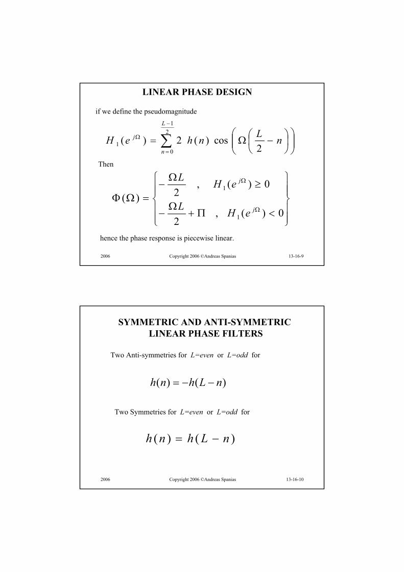
LINEAR PHASE DESIGN
if we define the pseudomagnitude
21
01 2
cos)(2)(
L
n
j nLnheH
Then
0)(,2
0)(,2)(
1
1
j
j
eHL
eHL
hence the phase response is piecewise linear.
2006 Copyright 2006 ©Andreas Spanias 13-16-10
SYMMETRIC AND ANTI-SYMMETRIC LINEAR PHASE FILTERS
Two Anti-symmetries for L=even or L=odd for
)()( nLhnh
)()( nLhnh
Two Symmetries for L=even or L=odd for
Page 6
2006 Copyright 2006 ©Andreas Spanias 13-16-11
EXAMPLES OF SYMMETRIES
nh 4L
0
nh
0
nh
0
nh
0
4L
3L
3L
2006 Copyright 2006 ©Andreas Spanias 13-16-12
EXAMPLES OF PHASE AND SYMMETRY IN h(n)
Normalized frequency (Nyquist == 1)0 0.1 0.2 0.3 0.4 0.5 0.6 0.7 0.8 0.9 1
-200
-150
-100
-50
0
50
Phas
e (d
egre
es)
0 0.1 0.2 0.3 0.4 0.5 0.6 0.7 0.8 0.9 1-200
-100
0
100
Normalized frequency (Nyquist == 1)
Pha
se(d
egre
es)
nh
0
nh
0
4L
4L
Page 7
2006 Copyright 2006 ©Andreas Spanias 13-16-13
Note that for )()( nLhnh
then )()( 1zHzzH L
Hence for L=odd and z = -1 then
)1()1()1( HH L
Thus the filter must have a zero at and is therefore notadequate for high-pass filtering.
HPF USING CERTAIN LINEAR PHASE FILTERS
2006 Copyright 2006 ©Andreas Spanias 13-16-14
Note that for )()( nLhnh
then )()( 1zHzzH L
Hence any L and z = 1 then
)1()1( HH
Thus the filter must have a zero at and is therefore notadequate for low-pass filtering.
0
LPF USING CERTAIN LINEAR PHASE FILTERS
Page 8
2006 Copyright 2006 ©Andreas Spanias 13-16-15
Design of FIR Digital FiltersLecture 14 - FIR DESIGN USING THE FOURIER SERIES
Andreas [email protected]
2006 Copyright 2006 ©Andreas Spanias 13-16-16
Design Using the Fourier Series
In filter design, there is an ideal transfer function Hd(z) that isapproximated by H(z). For example for a low-pass filter, an ideal frequency response is given below:
We like to minimize the mean square error, i.e.,
deHeH jjd
2)()(
21
zHd
c c
Page 9
2006 Copyright 2006 ©Andreas Spanias 13-16-17
Design Using the Fourier Series (Cont.)
Recalling that in general2
1
)()(n
ni
jij eiheH
then
deiheHn
ni
jijd
22
1
)()(2
1
Minimization of the integral above leads to an h(n) sequence that isprecisely equal to the sequence of Fourier series coefficients characterizing Hd(z). The resultant impulse response sequence is a sampled truncated sinc function.
2006 Copyright 2006 ©Andreas Spanias 13-16-18
Fourier Series Design Example
For the ideal low pass filter the impulse response sequence is an infinite length sampled sinc function. Lets say the sampling frequency is 8KHz and we wish to have a cutoff frequency at 2KHz. This results in
28000200022
s
cc f
f
That is
zHd
2n
2n
Page 10
2006 Copyright 2006 ©Andreas Spanias 13-16-19
Fourier Series Design Example (Cont.)The ideal impulse response hd(n) is given by
,...2,1,0,2
sinc21)( nnnh d
For an FIR filter of 11 coefficients
,...0,0,51,0,
31,0,1,
21,1,0,
31,0,
51,0,0...)(nh
This impulse response is not causal, however a shift operator of 5delays (z-5) will convert it into a causal one.
2006 Copyright 2006 ©Andreas Spanias 13-16-20
REALIZATION
. .5/1 3/1 /1 21/
...
.1z 1z 1z 1z 1z
1z 1z 1z 1z 1z
ny
nx
Page 11
2006 Copyright 2006 ©Andreas Spanias 13-16-21
Fourier Series Design Example (Cont.)
51,
31,1,
21,1,
31,
51
10865420 bbbbbbb
0 0.1 0.2 0.3 0.4 0.5 0.6 0.7 0.8 0.9 1-600
-400
-200
0
Normalized frequency (Nyquist == 1)
Pha
se (
degr
ees)
0 0.1 0.2 0.3 0.4 0.5 0.6 0.7 0.8 0.9 1-80
-60
-40
-20
0
20
Normalized frequency (Nyquist == 1)
Mag
nitu
de R
espo
nse
(dB
)
2006 Copyright 2006 ©Andreas Spanias 13-16-22
Fourier Series Design Example L=32
16,15,....0,....,15,16,2
)16(sinc21 nnbn
0 0.1 0.2 0.3 0.4 0.5 0.6 0.7 0.8 0.9 1-2000
-1500
-1000
-500
0
Normalized frequency (Nyquist == 1)
Pha
se (
degr
ees)
0 0.1 0.2 0.3 0.4 0.5 0.6 0.7 0.8 0.9 1-80
-60
-40
-20
0
20
Normalized frequency (Nyquist == 1)
Mag
nitu
de R
espo
nse
(dB
)
Page 12
2006 Copyright 2006 ©Andreas Spanias 13-16-23
Fourier Series Design Example L=64
32,31,....0,....,31,32,2
)32(sinc21 nnbn
0 0.1 0.2 0.3 0.4 0.5 0.6 0.7 0.8 0.9 1-3000
-2000
-1000
0
Normalized frequency (Nyquist == 1)
Pha
se (
degr
ees)
0 0.1 0.2 0.3 0.4 0.5 0.6 0.7 0.8 0.9 1-100
-50
0
50
Normalized frequency (Nyquist == 1)
Mag
nitu
de R
espo
nse
(dB
)
2006 Copyright 2006 ©Andreas Spanias 13-16-24
Truncating with Hamming Window L=64
Hamming(L)*2
)32(sinc21 nbn
0 0.1 0.2 0 .3 0.4 0 .5 0.6 0.7 0 .8 0.9 1-4000
-3000
-2000
-1000
0
Norm aliz ed frequenc y (Ny qu is t = = 1)
Pha
se (
degr
ees)
0 0 .1 0.2 0 .3 0.4 0 .5 0.6 0.7 0 .8 0.9 1-150
-100
-50
0
50
Norm aliz ed frequenc y (Ny qu is t = = 1)
Mag
nitu
de R
espo
nse
(dB
)
Page 13
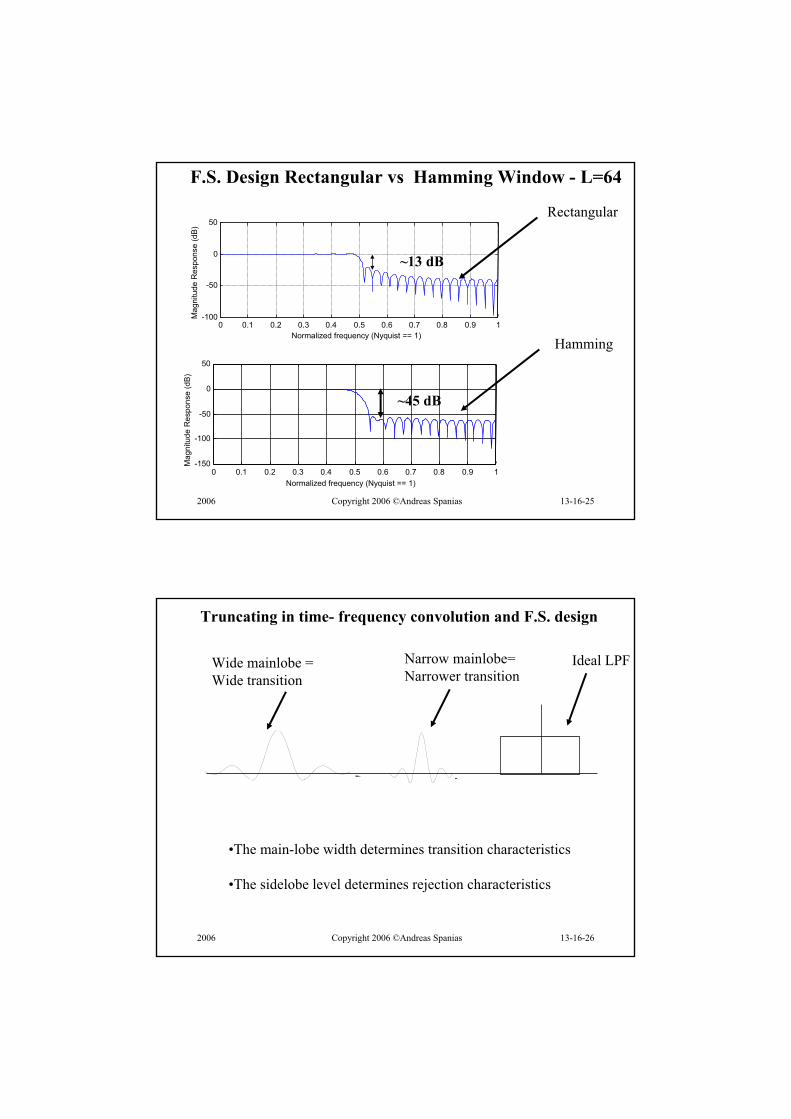
2006 Copyright 2006 ©Andreas Spanias 13-16-25
F.S. Design Rectangular vs Hamming Window - L=64
0 0.1 0.2 0.3 0.4 0.5 0.6 0.7 0.8 0.9 1-150
-100
-50
0
50
Normalized frequency (Nyquist == 1)
Mag
nitu
de R
espo
nse
(dB
)
0 0.1 0.2 0.3 0.4 0.5 0.6 0.7 0.8 0.9 1-100
-50
0
50
Normalized frequency (Nyquist == 1)
Mag
nitu
de R
espo
nse
(dB
)
Hamming
Rectangular
~45 dB
~13 dB
2006 Copyright 2006 ©Andreas Spanias 13-16-26
Truncating in time- frequency convolution and F.S. design
•The main-lobe width determines transition characteristics
•The sidelobe level determines rejection characteristics
Ideal LPFNarrow mainlobe=Narrower transition
Wide mainlobe =Wide transition
Page 14
2006 Copyright 2006 ©Andreas Spanias 13-16-27
Notes On Fourier Series Design
•The design performed in the previous example involved truncationof an ideal symmetric impulse response.A symmetric impulse response produces a linear phase response.
•Truncation involves the use of a window function which is multiplied with the impulse response. Multiplication in the time domain maps into frequency-domain convolution and the spectralcharacteristics of the window function affect the design.
•The main-lobe width determines transition characteristics
•The sidelobe level determines rejection characteristics
2006 Copyright 2006 ©Andreas Spanias 13-16-28
Design of FIR Digital FiltersLecture 15 - FIR DESIGN USING THE KAISER WINDOW
Andreas [email protected]
Page 15
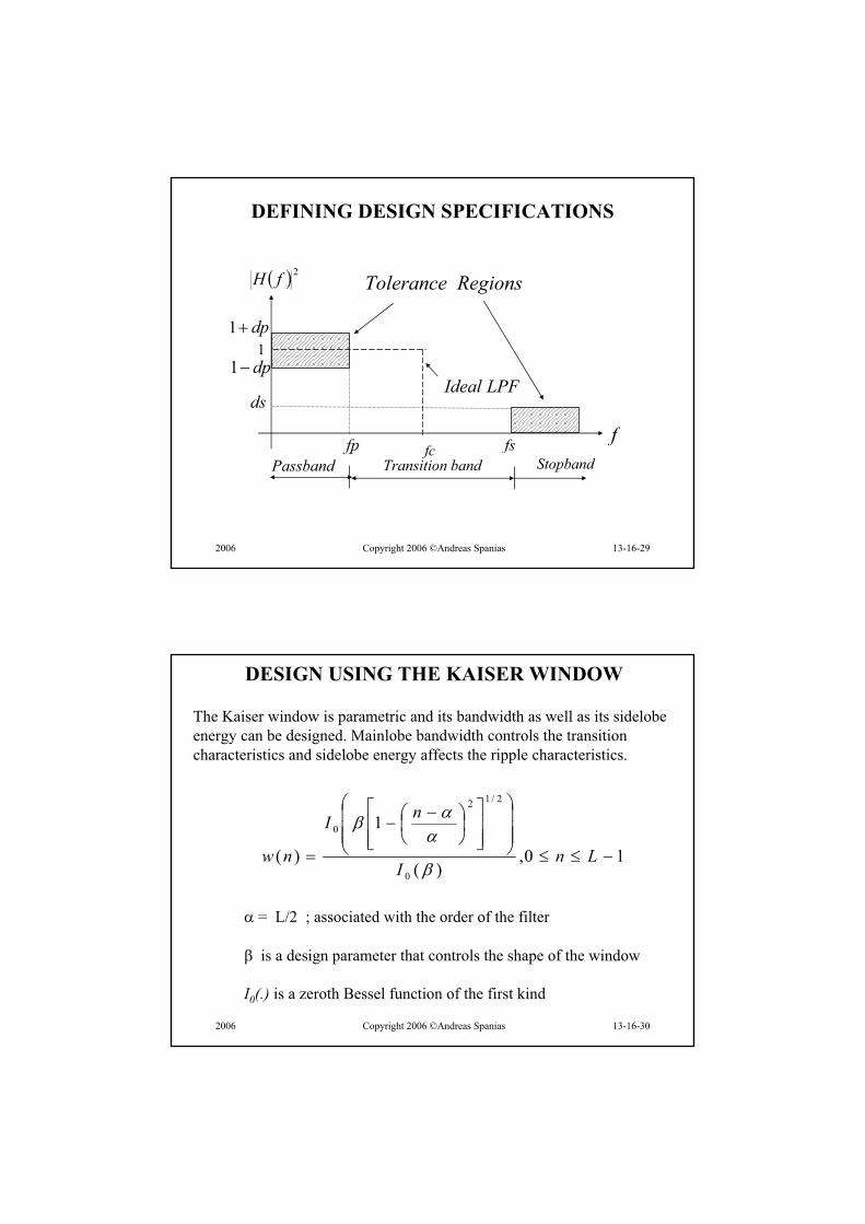
2006 Copyright 2006 ©Andreas Spanias 13-16-29
2fH
dp11dp1
dsLPFIdeal
ffp fcPassband bandTransition Stopband
RegionsTolerance
DEFINING DESIGN SPECIFICATIONS
fs
2006 Copyright 2006 ©Andreas Spanias 13-16-30
DESIGN USING THE KAISER WINDOW
The Kaiser window is parametric and its bandwidth as well as its sidelobeenergy can be designed. Mainlobe bandwidth controls the transition characteristics and sidelobe energy affects the ripple characteristics.
10,)(
1
)(0
2/12
0
LnI
nI
nw
= L/2 ; associated with the order of the filter
is a design parameter that controls the shape of the window
I0(.) is a zeroth Bessel function of the first kind
Page 16
2006 Copyright 2006 ©Andreas Spanias 13-16-31
DESIGN USING THE KAISER WINDOW (Cont.)
I xk
x k
k0
2
11
12
( )!
25 terms from the Bessel function are sufficient
2006 Copyright 2006 ©Andreas Spanias 13-16-32
EXAMPLES OF KAISER WINDOW
0 20 40 60 80 100 120 1400
0.1
0.2
0.3
0.4
0.5
0.6
0.7
0.8
0.9
1 0
1
Page 17
2006 Copyright 2006 ©Andreas Spanias 13-16-33
KAISER WINDOW DESIGN EQUATIONSGiven fp, fs, T and dp, ds determine the FIR filter coefficients.
TffA
dpds
ps )(2log20
),min(
10
The filter order is )2(285.2
8AL
0 1 1 0 2 8 7 5 00 5 8 4 2 2 1 0 0 7 8 8 6 2 1 2 1 5 00 2 1
0 4
. ( . ) ,
. ( ) . ( ) ,,
.
A AA A A
A
and the kaiser parameter is given by
2006 Copyright 2006 ©Andreas Spanias 13-16-34
DESIGN PROCEDURE
1. Determine the cutoff frequency for the ideal Fourier Seriesmethod.
ff f
cs p
22. Design the ideal LPF using the Fourier Series.3. Design the Kaiser window4. Shift and truncate the ideal impulse response
LnLnhnwnh dLPF 0,2
)()(
Note that this procedure can be generalized for the design of BPF, HPF, and BSF.
Page 18
2006 Copyright 2006 ©Andreas Spanias 13-16-35
Design by Zero-Placement
As zeros are placed towards the unit circle the frequency response magnitude decreases at and in the vicinity of the frequency of the zeros. .
o
o
foldover
2006 Copyright 2006 ©Andreas Spanias 13-16-36
Design by Zero-Placement
Example: Design a linear phase FIR filter for 60Hz interferencecancellation, that will pass a 10Hz signal of interest withoutattenuation. The sampling frequency is 500Hz.
256
500602
25500102
60
10
A second order filter is sufficient, since only a zero pair on the unit circle is required for 60Hz cancellation. The 10Hz responseis adjusted with a gain factor.
Page 19
2006 Copyright 2006 ©Andreas Spanias 13-16-37
Design by Zero-Placement (Cont.)
A linear phase (steady state) design means symmetric impulseresponse:
0)(
1)(606060
101010
2010
2010
jjj
jjj
ebebbeH
ebebbeH
and
77.2,9.1 10 bb
2006 Copyright 2006 ©Andreas Spanias 13-16-38
Design by Zero-Placement (Cont.)
0 0.1 0.2 0.3 0.4 0.5 0.6 0.7 0.8 0.9 1-50
0
50
100
150
Normalized frequency (Nyquist == 1)
Pha
se (
degr
ees)
0 0.1 0.2 0.3 0.4 0.5 0.6 0.7 0.8 0.9 1-60
-40
-20
0
20
Normalized frequency (Nyquist == 1)
Mag
nitu
de R
espo
nse
(dB
)
-1 -0.5 0 0.5 1
-1
-0.5
0
0.5
1
Real part
Imag
inar
y pa
rt
O
O
jjj eeeH 29.177.29.1)(
Page 20
2006 Copyright 2006 ©Andreas Spanias 13-16-39
Frequency Sampling Methods for FIR Filter design
The Frequency Sampling Method (FSM) involves: a) uniform sampling of a desired continuous frequency response function at Npoints, b) applying the N-point inverse Discrete Fourier Transformto obtain an N-point impulse response.
The FSM guarantees that the FIR frequency response matches that of the desired filter at the sampled points, however the response between the sampled points is different. If the desired filter function is due to an infinite impulse response then the FSM suffers also from time-domain aliasing.
2006 Copyright 2006 ©Andreas Spanias 13-16-40
Min-Max and Parks-McClellan Optimum FIR Design
The Parks-McClellan design is based on Min-Max
Equiripple and linear phase design is possible
This class of methods involve minimizing the maximum errorbetween the designed FIR filter frequency response and a prototype
)(maxmin,...,1,0),(
j
LiiheE
where
E e W e H e H ej jd
j j( ) ( )( ( ) ( ))
Page 21
2006 Copyright 2006 ©Andreas Spanias 13-16-41
FIR Filter Design Using MATLAB+
IN THE MATLAB SP TOOLBOX
cremez - Complex and nonlinear phase equiripple FIR filter design.fir1 - Window based FIR filter design - low, high, band, stop, multi.fir2 - Window based FIR filter design - arbitrary response.fircls - Constrained Least Squares filter design - arbitrary response.fircls1 - Constrained Least Squares FIR filter design - low and highpassfirls - FIR filter design - arbitrary response with transition bands.firrcos - Raised cosine FIR filter design.intfilt - Interpolation FIR filter design.kaiserord - Window based filter order selection using Kaiser window.remez - Parks-McClellan optimal FIR filter design.remezord - Parks-McClellan filter order selection.
+ MATLAB is registered trade mark of the MathWorks
2006 Copyright 2006 ©Andreas Spanias 13-16-42
FIR Filter Realizations
Direct Realizations L
i
ii zbzH
0
)(
...
...
nx
ny
1z 1z 1z
0b1b 2b 1Lb Lb
•Require multiply accumulate instructions
Page 22
2006 Copyright 2006 ©Andreas Spanias 13-16-43
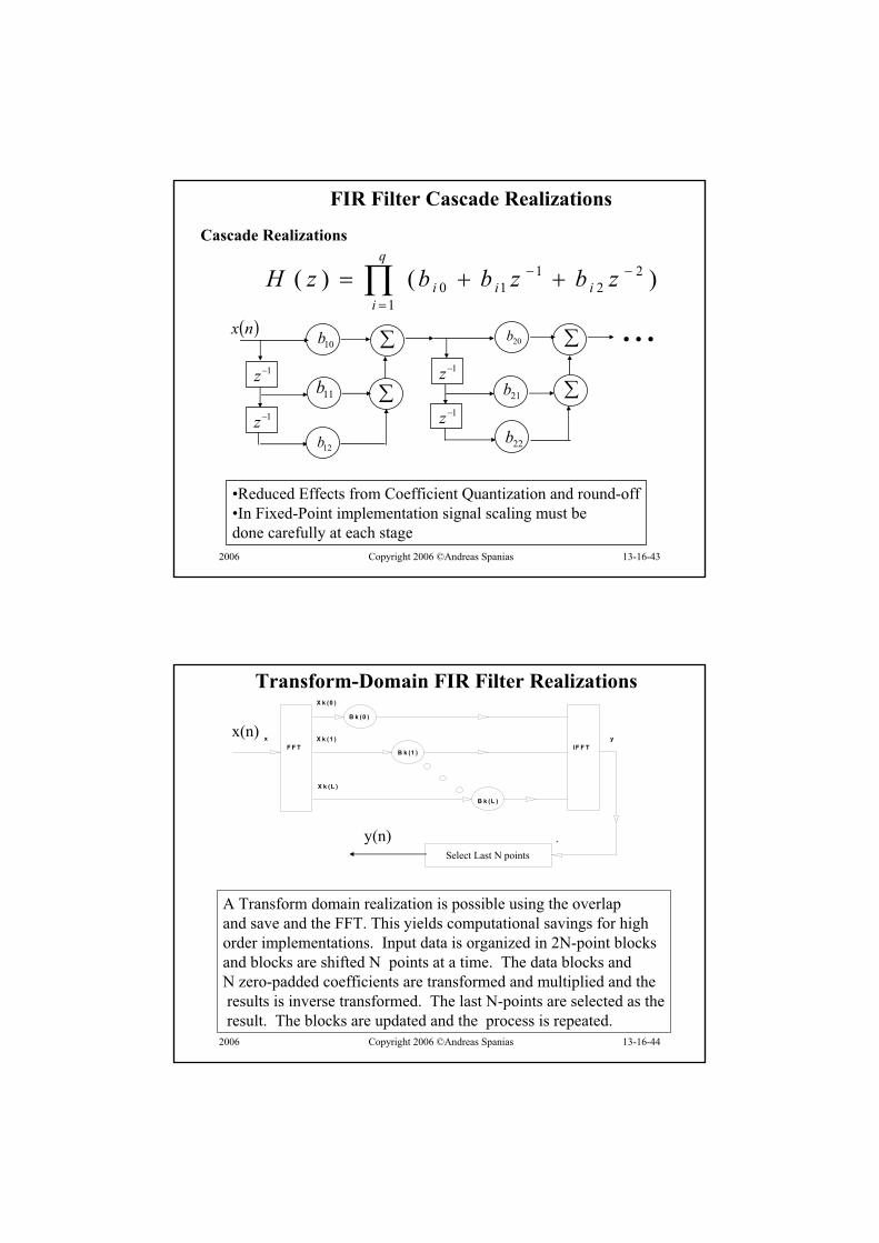
FIR Filter Cascade Realizations
Cascade Realizationsq
iiii zbzbbzH
1
22
110 )()(
...1z
1z
1z
1z
10b
11b
12b
20b
21b
22b
nx
•Reduced Effects from Coefficient Quantization and round-off•In Fixed-Point implementation signal scaling must be done carefully at each stage
2006 Copyright 2006 ©Andreas Spanias 13-16-44
Transform-Domain FIR Filter Realizations
A Transform domain realization is possible using the overlapand save and the FFT. This yields computational savings for highorder implementations. Input data is organized in 2N-point blocks and blocks are shifted N points at a time. The data blocks andN zero-padded coefficients are transformed and multiplied and theresults is inverse transformed. The last N-points are selected as theresult. The blocks are updated and the process is repeated.
F F T IF F Tx y
-
X k (0 )
X k (1 )
X k (L )
B k (0 )
B k (1 )
B k (L )
Select Last N points
x(n)
y(n)
Page 23
2006 Copyright 2006 ©Andreas Spanias 13-16-45
Transform-Domain FIR Filter Realizations (2)
Implements an N-th order filter with two 2-N point FFTs
For processing N points complexity is reduced fromO(N2) to O(Nlog2N)
F F T IF F Tx y
-
X k (0 )
X k (1 )
X k (L )
B k (0 )
B k (1 )
B k (L )
Select Last N points
x(n)
y(n)
2006 Copyright 2006 ©Andreas Spanias 13-16-46
Simple and Smart FIR Filter Realizations
L
i
izL
zH0
1)(
A simple L-tap filter can be built such that no multiplies are not used
This is a LPF with linear phase – if L is radix 2 the division can be implemented with shifts - below an example with L=16
0 0 . 1 0 . 2 0 . 3 0 . 4 0 . 5 0 . 6 0 . 7 0 . 8 0 . 9 1- 2 0 0
- 1 0 0
0
1 0 0
N o r m a l i z e d fr e q u e n c y ( N y q u i s t = = 1 )
Pha
se (
degr
ees)
0 0 . 1 0 . 2 0 . 3 0 . 4 0 . 5 0 . 6 0 . 7 0 . 8 0 . 9 1- 6 0
- 4 0
- 2 0
0
N o r m a l i z e d fr e q u e n c y ( N y q u i s t = = 1 )
Mag
nitu
de R
espo
nse
(dB
)
Page 24
2006 Copyright 2006 ©Andreas Spanias 13-16-47
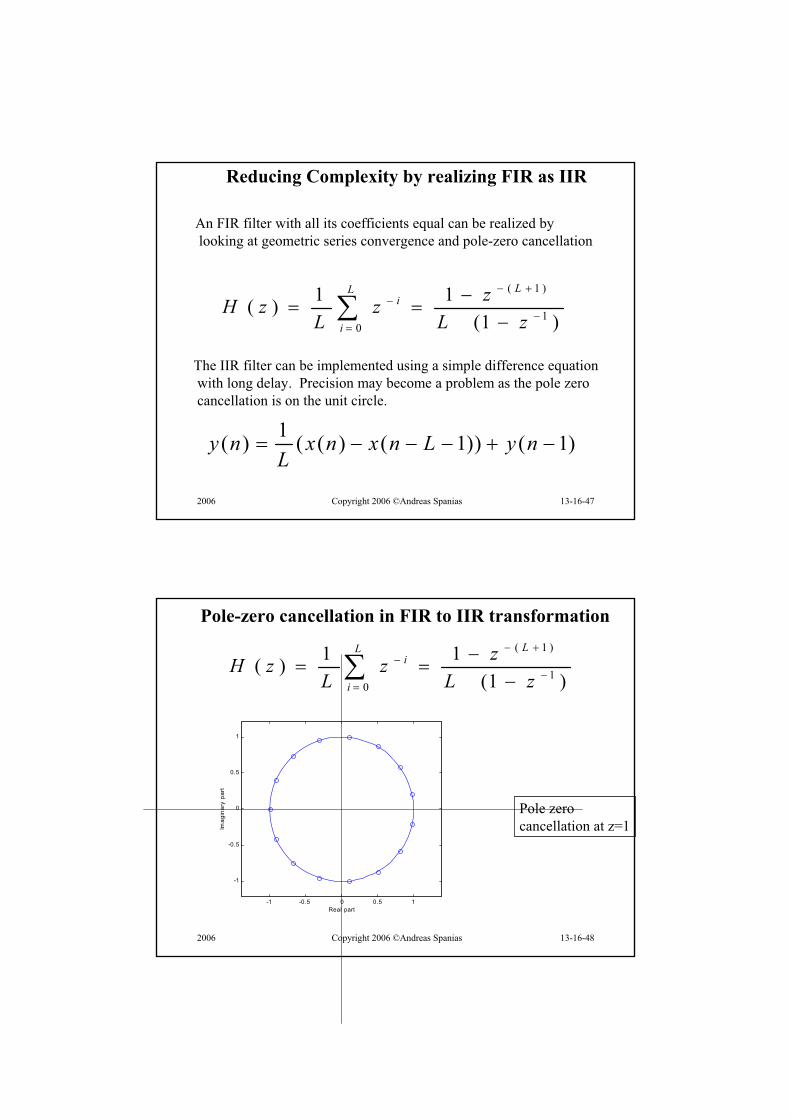
Reducing Complexity by realizing FIR as IIR
)1(11)( 1
)1(
0 zLzz
LzH
LL
i
i
An FIR filter with all its coefficients equal can be realized bylooking at geometric series convergence and pole-zero cancellation
The IIR filter can be implemented using a simple difference equationwith long delay. Precision may become a problem as the pole zerocancellation is on the unit circle.
1( ) ( ( ) ( 1)) ( 1)y n x n x n L y nL
2006 Copyright 2006 ©Andreas Spanias 13-16-48
Pole-zero cancellation in FIR to IIR transformation
)1(11)( 1
)1(
0 zLzz
LzH
LL
i
i
-1 -0.5 0 0.5 1
-1
-0.5
0
0.5
1
Real part
Imag
inar
y pa
rt
Pole zero cancellation at z=1
Page 25
2006 Copyright 2006 ©Andreas Spanias 13-16-49
Modifying Filter Response by Subtractive Operations
)()(1 jHPF
jLPF eHeH
__ =HPFLPFALL-PASS
c cc c
Using simple operations like this we can transform prototypeLPF to HPF or BPF, etc.
2006 Copyright 2006 ©Andreas Spanias 13-16-50
Implementing Efficiently Digital Cross-Over Using Subtractive Operations
LPF to tweeter
to wooferLinear Phase LPFWith delay L/2 samples
-+
could also implement delay compensation z –L/2
Page 26
2006 Copyright 2006 ©Andreas Spanias 13-16-51
Frequency Sampling
/20 /4
Ideal frequency response
N=16 samples
/40
Sampled ideal frequency response
/40
Interpolated frequency response
(a)
(b)
(c)
12 /
0( ) ( ) ( )k
Nj j kn N
d d dn
H k H e h n e
( ) ( ) 0 1dk
h n h n kN n N ; aliasing