DESIGN OF INTELLIGENT SPACECRAFT: AN INTERDISCIPLINARYENGINEERING EDUCATION COURSE

Abstract

This paper discusses a highly interdisciplinary course offered to students during the Spring 2007semester : Design of Intelligent Spacecraft. The course integrates concepts from mathematics,physics, engineering and computer science for the purpose of educating 4th year undergraduateand introductory masters-level students on the design of intelligent spacecraft. Course content isdivided into two pedagogically separate parts :

1. The historical development of physical models, including mathematical models for celestialmechanics and thermodynamics.

2. Application of these models for creating intelligent spacecraft, i.e., applications of thesemodels to pattern recognition, computer vision, and image processing. The first sectionintroduces physical mathematical models which, in the second section of the course, arere-visited to allow for model-based design.

In part (1), a new tact is taken for teaching the historical development of mathematics and physicsthat shapes the scientific view of the world today. Lectures seek to emphasize the rationale behindscientific thought through the variety of personalities that have defined it best characterized by thephrase :All science was new at some point. Specific classical topics include celestial mechanicsand thermodynamics which are introduced using excerpts from original works of the scientiststhat defined and revolutionized our understandings of thesefields. Some scientists consideredare Aristotle, Tycho, Kepler, Newton, Euler, Bernoulli, Fourier and other scientists relevant tocourse topics. Where possible, original manuscripts were provided and clarified by reformulatingthe work in modern terminology and mathematical notation. Historical content is complementedwith discussion on contemporary space missions relevant tothe discussion topic. For example,historical discussions on the discoveries of Cassini or Galileo includes discussions on the recentCassini-Huygens mission to Saturn. Further, these discussions include mission spacecraft type,its relevant design considerations and mission objectives. Discussion of mission objectives serveto highlight current boundaries of scientific knowledge andhow specific space missions seek tounderstand topics at these boundaries.

In part (2), students implemented programs relevant to spacecraft design. Programs included phys-ical simulations of celestial mechanics, thermodynamics,and signal processing programs for im-age manipulation and signal compression. Project topics reinforce topics covered in part (1) ofthe course. Results for physical simulations are compared against theoretically perfect results forthermodynamic simulations and established gold-standards from NASA’s HORIZONS system in

the case of celestial mechanics. Applications of these mathematical models in electrical engineer-ing lead to signal processing projects which motivate subsequent course topics on communication,image processing and image compression.

This paper includes successes, failures and lessons learned in teaching a course with such diversecontent and analyzes how well the mixture of history / engineering was received by the students.

Introduction

A new inter-disciplinary course,Design of Intelligent Spacecraft,was developed and taught dur-ing the 2007 academic year in at the University of North Carolina at Charlotte in the Departmentof Electrical and Computer Engineering (ECE). Successful spacecraft designed are predicated onthe ability for a wide variety of disciplines to contribute sets of compatible instruments and sys-tems which as a whole make up the spacecraft. The course introduces key design issues commonto deep-space spacecraft and focuses specifically on terrestrial spacecraft such as the Mars Ex-ploratory Rover (MER) Mission.

The course is not intended to directly address the mechanical issues associated with building ofspacecraft. Rather, students are provided conceptual background on the development of astronomy,space exploration, and introductory-level understandingof several prominent design issues thatmust be solved to design, build, and implement a successful robotic spacecraft.

The overall goal of the course is to introduce junior and senior level undergraduate students andfirst-year graduate students at the University of North Carolina at Charlotte to design issues relevantin building “intelligent” robotic spacecraft, i.e., spacecraft capable of completing complex missiontasks completely- or semi-automatically.

Since the audience for this course was primarily students within the ECE department, coursesections built up areas typically omitted from a ElectricalEngineering curriculum. Specifically,the course topics included : the history of astronomy and space exploration, the development ofmathematical models in the form of ordinary differential equations (ODEs) and partial differentialequations (PDEs), numerical methods to solve ODEs and PDEs,common spacecraft sensors andsystems, celestial mechanics and celestial navigation. Material for these topic come from a widevariety of courses in a number of different disciplines including : history, mathematics, physics,engineering and computer science.

As is typically the case for inter-disciplinary courses, there are formidable challenges in presentingthis material in an understandable way for the wide variety of students that may enroll for thecourse. Other challenges include instructing both historyand scientific theory simultaneously, andproviding a global perspective for the roles of each topics in the overall spacecraft design.

As mentioned earlier, the course is separated into two parts. The pedagogical content of thesesections is distinct and are as follows :

1. Topics in astronomy, mathematical modeling, and spacecraft design.

2. Numerical methods for modeling spacecraft design, applications of communications andoptical imaging to spacecraft design.

Section (1) comes first since it concentrates on introducingnew concepts and theory typicallyomitted from standard electrical engineering curriculum at both the undergraduate and graduatelevel. A new tact for teaching classical topics such as mechanics and thermodynamics is takenwhich uses source materials from the original manuscripts.Although, these manuscripts havelimited relevance in terms of modern terminology and notation for these subjects, the experimenthere is to evaluate if this new approach stimulates student interest in a subject which, in the typicalteaching context, may be dry and uninteresting. The centralconcept which I seek to convey tostudents is the realization thatAll science was new at some point.

With the vast attention to detail in many engineering classrooms, this truism is easily forgotten.This is reflected in the often omission of historical contextof topics in both engineering textsand lecture halls. Some texts1 make attempts to provide brief sketches of famous scientists whomade fundamental contributions to the discipline, yet these descriptions are often superficial incontent and rarely enter discussion in the classroom. The proposed course will use excerpts fromthe original publications written by the magnates of science and mathematics who have madefundamental contributions to modern science. Since this course will fall into the curriculum of theElectrical and Computer Engineering Department, emphasiswill be given to historical figures thatare both relevant to the course and relevant to topics from the core departmental curriculum.

Also as part of section (1), historical content is complemented with technical content on the fol-lowing topics :

• Development of astronomy from ancient times, starting withAristotle’s geocentric model ofthe universe.

– Key technical concepts : Observational astronomy : formingimages with telescopes,basics of telescope optics, and lenses. Theoretical astronomy : Copernicus’sDe revo-lutionibus orbium coelestiumand the development of the Helocentric theory

• Development of mathematics from ancient times, particularly its role as a tool to model thedynamics of heavenly bodies which came to define the field of celestial dynamics chieflythrough Newton’s universal theory of gravitation.

– Key technical concepts : Kepler’s Laws for planetary motion, Newton’s re-formulationof these laws as a natural consequence of his universal law ofgravitation. ODEs thatarise from Newtons universal law of gravitation. Thermodynamics and heat dissipationas modeled by a PDE.

Section (2) concentrates on the technical implementation of software algorithms needed to solvethe complex problems encountered when building robotic spacecraft. Discussion starts by exam-ining the difficulties that arise when we seek to obtain analytical solutions to the mathematicalmodels developed in section (1). This motivates the use of numerical methods for solving bothODEs and PDEs and the majority of this course section is dedicated to instructing students on theconcepts and implementation of these methods. In parallel to lecture, two-three week projects areassigned that require students to implement numerical techniques to address real-world problems.The projects follow:

1. Celestial mechanics : Modeling the Solar System using Runge-Kutta method to solve ordi-nary differential equations associated with the two-body problem (see §Appendix B: Celes-tial Mechanics Project).

2. Thermodynamics : Modeling Spacecraft Heat Dissipation using Euler’s method and theCrank-Nicolson method to solve 1-D and 2-D partial differential equations associated withheat dissipation (see §Appendix C: Thermodynamics Project).

3. Signal Processing : Image Formation, Extracting Structure from Images and Image Filteringfor Compression via Wavelet Filter Banks (see §Appendix D: Signal Processing Project).

Given that undergraduates and graduates are both enrolled in the course, different levels of exper-tise were required of students based on their enrollment status. For this reason, each project con-sisted of threetechnical levels.Higher technical levels required more proficiency with the coursematerial. Those students enrolled in the undergraduate section of the course needed to completeonly the first technical level within the assigned projects.Students enrolled in the master-levelgraduate section of the course were required to complete both the first and second technical lev-els. Students enrolled in the phd-level graduate section ofthe course were required to completeall three provided technical levels. Students enrolled in the undergraduate and master-level sec-tions were encouraged to attempt higher technical levels for extra credit. This stratification of theproject assignments was a very effective in allowing all students to work on the same topics whilebeing required to have different levels of proficiency commensurate to their enrollment status inthe course.

Textbook

As is often the case for inter-disciplinary courses, findingan appropriate text is extremely difficultand, in the final analysis, a course textbook was not adopted.As a result, source material for manyof the class topics include the entry “Lecture notes” which refer to note hand-compiled from a vastvariety of sources during course preparation in the Summer of 2006 (see §Class Topics). Manydifferent potential texts were considered primarily focusing on introductory astronomy texts asthese course concepts are a major component to the course. Specific texts considered as possiblesource texts included.2–4 Other contemporary texts were very valuable as study resources relevantto course topics such as5 and, of course, a large variety of original scientific manuscripts served assource material, especially for section (1), including.6–15

Two texts were read by students to complement lecture topics: Zero: The Biography of a Dan-gerous Idea,by Charles Seife16 andThe Mathematical Experience,by Phillip Davis and ReubenHersh.17 The first text discusses with the development of numbers, algebra, formal mathematicsand calculus accompanied by the historical forces that drove these developments. The second textdiscusses the mathematics and more advanced mathematical concepts including non-Cantorian settheory and the Reimann hypothesis.

Class Topics / Source Materials / Scoring Rubrics

As mentioned later in this paper (see §Lessons Learned) not all of the intended class topics werediscussed. In this section, those course topics covered in the course are discussed. The pedagogicalcontent of each topic is These topics differ slightly than those originally laid out in the coursesyllabus (see §Appendix A : Initial Course Syllabus). This section lists each of these topics (inbold) and, along with the topic, key concepts, relevant source material and scoring rubrics arelisted.

The history numbers the development of basic mathematics.Historical concepts: Rationalebehind the development of numbers, the development of algebra, development of different numbersystems, the history of the Arabic digits.Source material: Zero: The Biography of a DangerousIdea, by Charles Seife andThe Mathematical Experience,by Phillip Davis and Reuben Hersh.Rubrics: Test 1, Test 2, Final Examination, Quizzes and Homeworks.

Outer space and issues in spacecraft construction and system design. Technical concepts:What is space? Different types of spacecraft: flyby spacecraft, orbiter spacecraft, atmosphericspacecraft, lander spacecraft, rover spacecraft, penetrator spacecraft, observatory spacecraft, andcommunications spacecraft. Components to spacecraft: spacecraft cruise module, payload, andpropellant. Spacecraft systems: tracking, temperature control, power, communications, scienceinstruments.Source material: Lecture notes.Rubrics: Test 1, Test 2, Final Examination, Quizzesand Homeworks.

Scientists and their discoveries which contribute to current methods of space exploration.Historical concepts: Know the names, chronology, and achievements of scientists that have con-tributed to the development of course topics such as astronomy, telescope optics, celestial me-chanics, and thermodynamics.Source material: Lecture notes, original works:Opticks,IsaacNewton6andSidereus Nuncius (Sidereal Messenger),Galileo Galilei.11 Rubrics: Test 1, Test 2,Final Examination, Quizzes, and Homeworks.

Basic astronomical terminology Astronomical coordinate systems and development of celes-tial mechanics models.Technical concepts: Understand ephemeris variables, how to perform3-dimensional Euclidean transformations to express the position of points in different coordinatesystems, Kepler coordinates, Heliocentric Ecliptic Coordinates, Julian 2000.0 Coordinate System,International Celestial Reference Frame.Source material: Lecture notes, original works :Har-monices Mundi (Harmonies of the World),Johannes Kepler10 andThe Principia,Isaac Newton.7

Rubrics: Final Examination, Project 1.

Mathematical modeling and its application for prediction. Technical concepts:Using ODEsto develop an ephemeris that can predict the location of planets. Using PDEs to predict the tem-perature distribution within a space capsule exposed to a known constant surrounding temperature,i.e., boundary condition.Source material: Lecture notes.Rubrics: Project 1, Project 2.

Image formation for astronomy and telescope design, radiometry and simulation of lightpropagation. Technical concepts: The historical development of the telescope, refractive tele-scopes, Newtonian telescopes, Gregorian telescopes, Schmitt-Cassegrain telescopes, Ritchie-Chretientelescopes, basics of telescopic imaging and very-low power imaging. Digital image formation,sensors for image formation such as CCD and CMOS sensors.

Thermodynamic issues in spacecraft design for deep space exploration. Technical concepts:Thermodynamics, heat dissipation, the heat equation, the divergence theorem

Gravitation, Escape Velocity. Technical concepts: Newtons Three Laws of Motion, gravity,universal law of gravitation, propulsion, energy to mass ratio

Celestial Mechanics.Technical concepts: Kepler’s Laws, Ordinary Differential Equations arisingfrom the two-body gravitational problem, NASA’s development of an online Ephemeris and how itmay be used, extensions to the two-body model and improved models of the dynamics of our solarsystem through the secular variations of the planetary orbits (VSOP82 and VSOP87).

Celestial Navigation. Technical concepts: Stationary points of the two-body model, Librationpoints, the Interplanetary Transport Network (ITN), Spacecraft propulsion, Hohmann transfer or-bit, Gravitational slingshot.Source materials: Lecture notes.Rubrics: Test 1, Test 2, FinalExamination.

Numerical Methods for solving Ordinary Differential Equat ions. Technical concepts : Runge-Kutta method for integrating the ordinary differential equation governing the two-body gravita-tional problem.Source materials: Numerical Recipes in C,Press, Teukolsky, Vetterling and Flan-nery.5 Rubrics: Project 1, Test 2.

Numerical Methods for solving Partial Differential Equati ons. Technical concepts: Applyingfinite difference methods for solving PDEs with the specific example of the heat diffusion equation.Explicit methods including forward Euler scheme in both 1 dimension and 2 dimensions. Implicitmethods including the Crank-Nicholson scheme in both 1 dimension and 2 dimensions.Sourcematerials: Time Dependent Problems and Difference Methods, Gustafsson Kreiss and Oliger,18

Numerical Recipes in C,Press, Teukolsky, Vetterling and Flannery.5 Rubrics: Project 2, FinalExamination.

Computer Usage

Students design, simulate, and analyze a variety of projects emphasizing image processing andcomputer vision as it applies to solving difficult problems in deep space exploration spacecraftdesign. MATLAB should be accessible as a tool for completingprojects.

From a first-day class survey (see §Teaching the Course), it was apparent that many of the studentshad not been exposed to MATLAB programming. Hence, an initial tutorial in-class was providedand several supporting resources were made available through the course website.

Grading Measures

Quantitative measures of student aptitude in the various course concepts were measured using ex-aminations, oral presentations, homeworks, in-class quizzes, and computer programming projects.This section details the method used in applying each measure and presents student performance ineach category. Some discussion is provided to detail trendsand other notable observations relevantto the measurement and student performance.

0 20 40 60 80 1000

2

4

6

8

0 20 40 60 80 1000

2

4

6

8

0 20 40 60 80 1000

2

4

6

8

(a) Test 1 (b) Test 2 (c) Final Exam

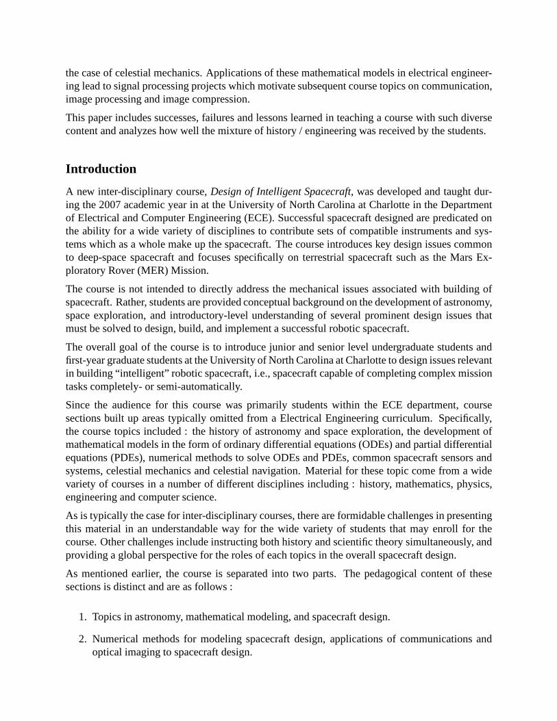
Figure 1: Plots (a-c) above show histograms of the students performance on the three tests ad-ministered over the course of the semester. Each test consisted of approximately 50% historical /conceptual questions and 50% technical questions. Students showed improved their performanceon tests over the semester.

Examinations

One measure of student proficiency in course topics was provided by midterm and final examina-tions. These examinations give nearly equal weight to historic and technical course concepts withslightly more emphasis on technical topics.

As one can see from Fig. 1, the students struggled on the first test. It is most likely that this maybe attributed to the fact that most students had not previously taken courses with the instructor andthat they were not familiar with the examination style of theinstructor or accustomed to the degree

Undergraduate Student Scores

0 20 40 60 80 1000

1

2

3

4

5

0 20 40 60 80 1000

1

2

3

4

5

0 20 40 60 80 1000

1

2

3

4

5

0 20 40 60 80 1000

1

2

3

4

5

(a) Midterm History (b) Midterm Technical (c) Final History (d) Final Technical

Graduate Student Scores

0 20 40 60 80 1000

2

4

6

0 20 40 60 80 1000

2

4

6

0 20 40 60 80 1000

2

4

6

0 20 40 60 80 1000

2

4

6

(e) Midterm History (f) Midterm Technical (g) Final History (h) Final Technical

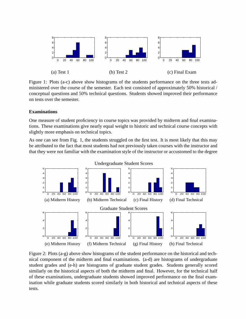
Figure 2: Plots (a-g) above show histograms of the student performance on the historical and tech-nical component of the midterm and final examinations. (a-d)are histograms of undergraduatestudent grades and (e-h) are histograms of graduate studentgrades. Students generally scoredsimilarly on the historical aspects of both the midterm and final. However, for the technical halfof these examinations, undergraduate students showed improved performance on the final exam-ination while graduate students scored similarly in both historical and technical aspects of thesetests.

0 20 40 60 80 1000

2

4

6

8

0 20 40 60 80 1000

2

4

6

8

0 20 40 60 80 1000

2

4

6

8

(a) Presentation 1 (b) Presentation 2 (c) Homeworks

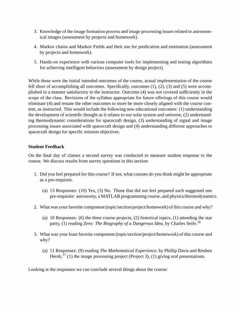
Figure 3: (a,b,c) Show histogram plots of student grades fortwo presentations and the overallhomework average computed from five homeworks completed during the semester. Students im-proved their performance on presentations from (a) to (b). The performance on homeworks issomewhat lower reflecting the fact that homeworks typicallyhave a higher degree of difficulty.

of proficiency on the course materials expected by the instructor. This hypothesis agrees with thegeneral trend observed from (a-c) which shows students steadily improving their test scores.

Homeworks / Quizzes

When projects and presentations are not assigned, homeworkassignments are provided to developstudent proficiency in lecture topics and quizzes encouragedeveloping these proficiencies in-syncwith their presentation in lecture. During the course of thesemester three homeworks were as-signed and five quizzes were conducted.

Peer-Reviewed Presentations

Each student provided two presentations and associated written reports during the first half of thecourse. The first presentation had each student focus on a specific scientist of significance that hasmade one or more significant contributions to topics of interest for the course. The second and thirdpresentations required each student to read a contemporaryresearch article related to astronomy,or space exploration.Sciencewas often used as an appropriate source since it’s articles are writtento be understandable to a wide readership. Students were asked to present the topic of the researcharticle, the significance of the research and findings in the article and the background informationnecessary to clarify the significance of the research results.

Student presentations were rated by other students using peer review sheets. The review sheet al-lowed each student to rate the presentation on a 5 point scale. A rubric was adopted that assignedthe overall presentation score to be the average overall score from the student peer-review com-bined with the instructors rating of the presentation with a40-60 percent weighting respectively.

From Fig. 3, one can see that students had mixed results in theinitial presentation and better resultsin the second presentation. The overall homework average shown in plot (c) reflects the fact thathomeworks had a higher degree of technical difficulty. Proficiency on such homework problemsprepare students to improve their performance on measures that more significantly impact theirgrade such as examinations and projects.

0 20 40 60 80 1000

2

4

6

8

0 20 40 60 80 1000

2

4

6

8

0 20 40 60 80 1000

2

4

6

8

(a) Project 1 (b) Project 2 (c) Project 3

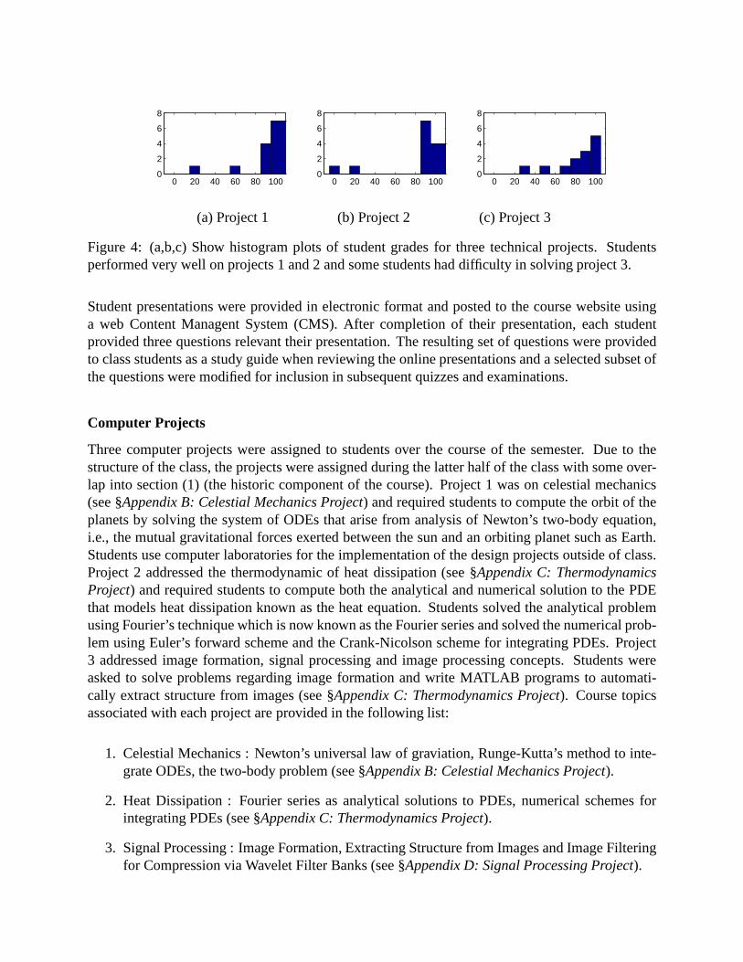
Figure 4: (a,b,c) Show histogram plots of student grades forthree technical projects. Studentsperformed very well on projects 1 and 2 and some students had difficulty in solving project 3.

Student presentations were provided in electronic format and posted to the course website usinga web Content Managent System (CMS). After completion of their presentation, each studentprovided three questions relevant their presentation. Theresulting set of questions were providedto class students as a study guide when reviewing the online presentations and a selected subset ofthe questions were modified for inclusion in subsequent quizzes and examinations.

Computer Projects

Three computer projects were assigned to students over the course of the semester. Due to thestructure of the class, the projects were assigned during the latter half of the class with some over-lap into section (1) (the historic component of the course).Project 1 was on celestial mechanics(see §Appendix B: Celestial Mechanics Project) and required students to compute the orbit of theplanets by solving the system of ODEs that arise from analysis of Newton’s two-body equation,i.e., the mutual gravitational forces exerted between the sun and an orbiting planet such as Earth.Students use computer laboratories for the implementationof the design projects outside of class.Project 2 addressed the thermodynamic of heat dissipation (see §Appendix C: ThermodynamicsProject) and required students to compute both the analytical and numerical solution to the PDEthat models heat dissipation known as the heat equation. Students solved the analytical problemusing Fourier’s technique which is now known as the Fourier series and solved the numerical prob-lem using Euler’s forward scheme and the Crank-Nicolson scheme for integrating PDEs. Project3 addressed image formation, signal processing and image processing concepts. Students wereasked to solve problems regarding image formation and writeMATLAB programs to automati-cally extract structure from images (see §Appendix C: Thermodynamics Project). Course topicsassociated with each project are provided in the following list:

1. Celestial Mechanics : Newton’s universal law of graviation, Runge-Kutta’s method to inte-grate ODEs, the two-body problem (see §Appendix B: Celestial Mechanics Project).

2. Heat Dissipation : Fourier series as analytical solutions to PDEs, numerical schemes forintegrating PDEs (see §Appendix C: Thermodynamics Project).

3. Signal Processing : Image Formation, Extracting Structure from Images and Image Filteringfor Compression via Wavelet Filter Banks (see §Appendix D: Signal Processing Project).

Overall Grading Rubric

Grades are determined by performance on exams, homeworks, projects, and in-class presentations.The weight of each item in determining the final grade is as follows: Homeworks 15%, Projects35%, Presentations 30%, and Exams 20%.

Teaching the Course

Enrollment for the course was open to all junior, senior and graduate students with the pre-requisiteof “Permission of Department” which required the consent ofthe instructor for enrollment. Evenwith this somewhat awkward requirement for course registration, enrollment for such an electivecourse was atypically high and included 15 students overallwith 8 undergraduate students and 7graduate students. Attending students were primarily Electrical and Computer Engineering majorswith the exception of three students that had majors in Mechanical Engineering, Physics, andEngineering Technology. Classroom content consisted of two 75-minute lectures each week. Muchof the course material was compiled from a variety of sourcesso class attendance, while not figuredinto the final course grade, was very important for students to obtain the class notes and keep pacewith the class topics.

First Day Survey

During the first lecture, a survey was conducted to determinethe student demographics and theirbackgrounds. The survey determined that underlying interests and technical proficiency of classstudents. Survey data indicated that most students had taken a course in signals and systems(sometimes referred to as linear systems) and about a third of the students had taken digital signalprocessing. These courses build mathematical modeling skills which play a significant role in thetechnical aspects of the course. However, it was an experiment to not require one or both of thesecourses as pre-requisites. About two-thirds of the students had not been exposed to MATLAB pro-gramming which is required to complete the three course projects and some of the assigned home-work problems. An in-class MATLAB programming tutorial anda host of supporting materialswere provided to empower students to complete their programming assignment (see §ComputerUsage).

Outcomes

According to the initial syllabus (see §Appendix A : Initial Course Syllabus), the following com-petencies should be imparted to the students:

1. An understanding of the mathematical history of astronomy and electrical engineering (as-sessment by tests/homework).

2. A basic understanding of astronomy including Kepler’s laws and their historical development(assessment by projects,tests, and homework)

3. Knowledge of the image formation process and image processing issues related to astronom-ical images (assessment by projects and homework).

4. Markov chains and Markov Fields and their use for predication and estimation (assessmentby projects and homework).

5. Hands-on experience with various computer tools for implementing and testing algorithmsfor achieving intelligent behaviors (assessment by designproject).

While these were the initial intended outcomes of the course, actual implementation of the coursefell short of accomplishing all outcomes. Specifically, outcomes (1), (2), (3) and (5) were accom-plished in a manner satisfactory to the instructor. Outcome(4) was not covered sufficiently in thescope of the class. Revisions of the syllabus appropriate for future offerings of this course wouldeliminate (4) and restate the other outcomes to more be more closely aligned with the course con-tent, as instructed. This would include the following new educational outcomes: (1) understandingthe development of scientific thought as it relates to our solar system and universe, (2) understand-ing thermodynamic considerations for spacecraft design, (3) understanding of signal and imageprocessing issues associated with spacecraft design and (4) understanding different approaches tospacecraft design for specific mission objectives.

Student Feedback

On the final day of classes a second survey was conducted to measure student response to thecourse. We discuss results from survey questions in this section:

1. Did you feel prepared for this course? If not, what coursesdo you think might be appropriateas a pre-requisite.

(a) 13 Responses: (10) Yes, (3) No. Those that did not feel prepared each suggested onepre-requisite: astronomy, a MATLAB programming course, and physics/thermodynamics.

2. What was your favorite component (topic/section/project/homework) of this course and why?

(a) 10 Responses: (6) the three course projects, (2) historical topics, (1) attending the starparty, (1) readingZero: The Biography of a Dangerous Idea,by Charles Seife.16

3. What was your least favorite component (topic/section/project/homework) of this course andwhy?

(a) 11 Responses: (9) readingThe Mathematical Experience,by Phillip Davis and ReubenHersh,17 (1) the image processing project (Project 3), (1) giving oral presentations.

Looking at the responses we can conclude several things about the course:

• Most students felt prepared for the course.Although three responses indicated a need for other coursesthe vast majority of studentswere able to deal with the concepts as presented in class and were able to demonstrate theirunderstanding in the various quantitative measures (see §Grading Measures). This is animportant outcome as there were initially some concern about the variety of students whichwere allowed to enroll in the course.

• Students preferred the assigned project work.Question 2 from the survey indicates that the projects were the most popular aspect of thecourse. In course projects, students are asked to implementa program to accomplish tech-nical goals. Hence, these are essentially technical aspects of the course which makes onequestion whether the role of historical contents within theclass. The historical aspects ofthe course are represented explicitly with two students mentioning the historical lectures andone mentioning Seife’s book on mathematical history.

• Students did not like the second text accompanying the course.With nine student responses, it is clear that the inclusion of Davis and Hersh’s book, TheMathematical Experience, was not popular with the students. The content of this book isprimarily an editorial on the philosophy of mathematics andmathematical modeling. Whilethis is a component of the course content, it is likely that this text will not be included infuture teachings of this course.

Lessons Learned

Student feedback and the experience of teaching this coursefor the first time has provided valu-able lessons. The first lesson is that the course tried to include too much new material for asingle-semester course, especially considering the lack of a prerequisite for student enrollmentand the fact that both undergraduate and graduate students may enroll in the course. These weremajor contributing factors that made it impossible to satisfactorily cover the final section of thecourse (see §Outcomes). The specific topic of interest omitted was Markov random fields andtheir application to performing automated tasks from sensed image data. This topic was to extendthe discussion on image and signal processing to include howintelligent machines can use thesemodels for decision-making. Example applications of such models include detecting obstacles forterrestrial navigation, i.e., finding rocks or hazardous terrain, or recognizing landmarks in imagesfor self-localization, i.e., determining where in space oron the planet surface the craft is located.Given that the class prerequisites are not changed, it is likely that outcome (4) will be removedfrom the syllabus in future offerings of this course.

Unfortunately, measured results do not produce conclusiveevidence that the inclusion of histori-cal course content stimulates student interest, motivation, or performance in the classroom. Thelargest impediment to such analysis is the sample size of 15 total students. A more conclusivestatement could be made given a larger enrollment. While thestudent feedback supports the ideathat historical context allows students to better understand why they are learning a given topic,it is not clear that they learn that topic better or are motivated to be more interested in the topicafter being made aware of the history behind the concepts. More data and analysis of that data isnecessary to show that this is the case for this interdisciplinary course.

Conclusions

This paper has described a new interdisciplinary course that marries the instruction of at least fivedifferent disciplines in a unique way. Course content is intended for upper level undergraduateand introductory graduate students and seeks to expose these students to concepts in astronomy,history, mathematical modeling, physics and engineering.Course content was taken from a num-ber of different contemporary and historical manuscripts which was intended to stimulate studentinterest. No significant conclusions can be made regarding the impact of these materials on studentproficiencies on course outcomes. Yet, positive student feedback on the historical course materialsindicate that there may be a link between these materials andachieving course outcomes. Hence,teaching this course provided new insights regarding the inclusion of historical topics in engineer-ing courses. In addition, this paper presents effective rubrics for oral presentations and effectivetechniques for designing projects that may be completed by both undergraduate and graduate, i.e.,students with different enrollment status. The large enrollment for the course (15) relative to thattypically observed in other undergraduate/graduate elective courses (4-5) indicates a significantamount of student interest exists in the topic.

The concepts discussed in the class not only develop studentskill in the design of spacecraft andspacecraft instrumentation but also are applicable outside this context. In fact, topics proposedfor discussion in class are also used in industry for file compression,19 image segmentation,20,21

robotics and numerous other contexts as described in texts.21 Lecture notes, presentations, lab-oratories, and visual media generated for the purpose of instructing this course is provided viathe university web site (http://www.visionlab.uncc.edu=⇒ Courses Link). This is an extremelyeffective way to disseminate the course content to other universities both local and international.

The authors of this paper would like to acknowledge the NorthCarolina Spacegrant Consortium(NC Spacegrant) which provided funds via their Higher Education Program to sponsor the devel-opment of this course.

References

1. D. E. Johnson, J. R. Johnson, and J.L. Hilburn,Electric Circuit Analysis, Wiley, 1997.

2. Neil F. Comins,Discovering the Universe, W. H. Freeman and Company, seventh edition edition, 2005.

3. M. T. Brück, Exercises in Practical Astronomy using Photographs: with solutions, IOP PublishingLtd., 1990.

4. AAAS and NASA,Exploring the Inner Solar System : Expecting the Unexpected, AAAS Publishing,2006.

5. William H. Press, Saul A. Teukolsky, William T. Vetterling, and Brian P. Flannery,Numerical Recipesin C: The Art of Scientific Computing, Cambridge University Press, second edition edition, 1992.

6. Isaac Newton,Opticks, or A Treatise on the Reflections, Refractions, Inflexions and Colours of Light,Printed by Ben Walford, 1704.

7. Isaac Newton,Principia Mathematica, 1687.

8. Pierre-Simon Laplace,A Philosophical Essay on Probabilities, Dover Publications, 1996.

9. Pierre-Simon Laplace,Celestial mechanics / Pierre Simon Laplace. Translated, with a commentary byNathaniel Bowditch, Chelsea Pub. Co, 1966.

10. Johannes Kepler,Harmonices Mundi, 1619.

11. Galileo Galilei,Sidereus Nuncius, 1610.

12. Carl F. Gauss, W.C. Waterhouse, J. Brinkhuis, C. Greiter, A.W. Grootendorst, and Arthur A. Clarke,Disquisitiones Arithmeticae, Springer, 1986.

13. Joseph Fourier,The Analytical Theory of Heat, Dover Publications, 2003.

14. Leonhard Euler and J.D. Blanton,Introduction to Analysis of the Infinite : Book I, Springer, 1988.

15. Nicolaus Copernicus,De revolutionibus orbium coelestium, 1543.

16. Charles Seife,Zero: The Biography of a Dangerous Idea, Penguin Books, 2000.

17. Phillip J. Davis and Reuben Hersh,The Mathematical Experience, Mariner Books, 1999.

18. Bertil Gustafsson, Heinz-Otto Kreiss, and Joseph Oliger, Time Dependent Problems and DifferenceMethods, Wiley-Interscience, 1995.

19. Bober M. Mokhtarian, F.,Curvature Scale Space Representation: Theory, Applications, and MPEG-7Standardization, Springer, 2003.

20. S. Geman and D. Geman, “Stochastic Relaxation, Gibbs Distributions, and the Bayesian Restoration ofImages,” IEEE Transactions on Pattern Analysis and Machine Intelligence, vol. 6, no. 6, pp. 721–741,1984.

21. Stan Z. Li,Markov Random Field Modeling in Image Analysis, Springer, 2001.

Appendix A : Initial Course Syllabus

UNC Charlotte Machine Vision Lab - ECGR3090/6090/8090 Syllabus http://www.visionlab.uncc.edu/index2.php?option=com_content&task=...

1 of 2 12/18/2007 05:07 PM

ECGR3090/6090/8090 SYLLABUS

Written by Andrew Willis Wednesday, 03 January 2007

Syllabus

ECGR3090/ECGR6090/ECGR8090 - Seminar Course : Design of Intelligent Spacecraft (3)

Catalog Data The course builds upon and synthesizes knowledge from the engineering science, mathematics, and physical sciences stem of core curriculum. The specific topics teach engineering analysis, synthesis, and design, while simultaneously affording an opportunity for the students to investigate an area of specialization. May be repeated for credit.

Lecture Times Monday and Wednesday 12:30 p.m. - 1:45 p.m.

Lecture Room Woodward Hall 125

Reference No required text.

Additional Reference

Discovering the Universe 7th edition, Comins and Kaufmann III, Freeman, 2005.Astronomy 5th Edition, Chaisson and McMillan, Pearson Prentice-Hall, 2007.

Goals The objective of this course is to provide students with a working knowledge pf algorithms andtechniques used in designing intelligent spacecraft, i.e., robotic systems which can autonomously perform complex space-mission tasks.

Prerequisite Permission of the Department

Class TopicNumbers and their historyBiographies of mathematicians responsible for developing core electrical engineering and signal processing concepts.Basic astronomical terminologyAstronomical coordinate systems and development of celestial mechanics modelsMathematical modeling and its application for predictionImage formation for astronomy and telescope designRadiometry and Simulation of light propagationShading and InterreflectionTracking, Structure from motionIssues in spacecraft design for deep space exploration.

OutcomesThe following competencies should be imparted to the students: 1. An understanding of the mathematical history of astronomy and electrical engineering (assessment by homework). 2. A basic understanding of astronomy including Kepler's laws and their historical development (assessment by projects and homework) 3. Knowledge of the image formation process and image processing issues related to astronomical images (assessment by projects and homework).4. Markov chains and Markov Fields and their use for predication and estimation (assessment by projects and homework).5. Hands-on experience with various computer tools for implementing and testing algorithms for achieving intelligent behaviors (assessment by design project).

Computer Usage Students design, simulate, and analyze a variety of projects emphasizing image processing and computer vision as it applies to solving difficult problems in deep space exploration spacecraft design. MATLAB should be accessible as a tool for completing projects.

Laboratory Students use computer laboratories for the implementation of the design projects outside of class.

Design Content The design projects for the course vary from semester to semester.

Grading *Grades are determined by performance on exams, homeworks, projects, and in-class presentations. The weight of each item in determining the final grade is as follows: Homeworks 15%Projects 35%Presentations 30%Exams 20%

Follow-up Courses N/A

Academic Integrity Students have the responsibility to know and observe the requirements of the UNCC Code of Student Academic Integrity (2001-2003 UNCC Catalog, p. 275) . This code forbids cheating, fabrication or falsification of information, multiple submission of academic work, plagiarism, abuse of academic materials, and complicity in academic dishonesty.

Notes Semester syllabus will be provided to the students on the first day of class.

Coordinator A. Willis, Professor of Electrical & Computer Engineering

Appendix B: Celestial Mechanics Project

Project 1 : Celestial Mechanics

This project will familiarize the student with solving Newton’s equations for the motion of theheavenly bodies. This document describes 3 technical levels of completion for the project. ForECGR3090 students, only the first technical level needs to becompleted. For ECGR6090 stu-dents, both the first and second technical levels need to be completed. For ECGR8090 students alltechnical levels should be completed. Extra credit will be extended to students that complete tech-nical levels beyond their enrolled status in the course.Please indicate if your project is intendedto include extra credit work.

Technical Level 1

Using MATLAB, implement a model of the Earth’s orbit around the sun using as initial data valuesfor position and velocity taken from the textfileearthmoon.txtobtained from NASA’s Jet Propul-sion Laboratory (JPL) Horizons project. The model should plot the orbit of the Earth using onlythe 2-dimensional (x,y) coordinates of the Earth. The differential equations of motion should besolved using your implementation of the 4th order accurate Runge-Kutta scheme.

To turn in :

1. Turn in a plot of the Earth’s orbit over a 5 year interval using your solution and using theanalytic solution.

2. Turn in a plot showing the error between the Earth’s orbit as represented by Kepler’s analyticsolution and the solution computed using Runge-Kutta numerical integration. To do so, findthe minimum distance between each computed Kepler orbital position and the closest orbitalposition of the Earth using the Runge-Kutta method. Plot themagnitude of this differenceas a function of the position index.

3. Turn in a plot of the error magnitudes between your computed positions for the Earth andthe positions computed by JPL using the Horizons program forthe time interval January 1,2000 to January 1, 2005. Here, your x-axis should be the pointindex for each of the JPLdata points and the y-axis should be the minimum distance between a specific JPL data pointand the points computed from Runge-Kutta integration.

4. Turn in your MATLAB code.

5. Turn in a discussion of what you observe from the plots generated in (1) and (2).

Technical Level 2

Extend the results from technical level 1 to 3-dimensional space and add Jupiter, Mars, Venus andSaturn. Initial positions and velocities of these planets are available from textfiles that bear theplanet name, e.g.,venus.txt.

To turn in :

1. Turn in a single plot showing the orbits of all the planets over a 5 year interval using yoursolution.

2. Turn in a plot that compares your solution to Kepler’s analytic solution for each of the planetby plotting both solutions and taking the difference of the length of the position vectors.(Similar to that from Technical Level 1, but the vectors are now 3D).

3. Turn in a plot which shows, as different traces, the error magnitudes between your computedpositions for each of the planets and the positions computedby JPL using the Horizonsprogram for the time interval January 1, 2000 to January 1, 2005. The plot should also havea legend. (Similar to that from Technical Level 1, but the vectors are now 3D).

4. Turn in your MATLAB code.

5. Turn in a discussion of what you observe from the plots generated in (1) and (2).

Technical Level 3

Extend the results from technical level 2 and add Mercury to the 3-dimensional solar systemmodel. Read, understand and incorporate corrections associated with relativistic effects as de-scribed in Aldo Vitagliano’s paper”Numerical integration for the real time production of funda-mental Ephemerides over a wide time span”(ask for additional handout regarding this problem).

To turn in :

1. Turn in a single plot showing the orbits of all the planets over a 5 year interval using yoursolution and using the analytic solution.

2. Turn in a plot that compares your solution to Kepler’s analytic solution for each of the planetby plotting both solutions and taking the difference of the length of the position vectors.(Similar to that from Technical Level 2).

3. Turn in a plot of the error magnitudes between your computed positions for each of theplanets and the positions computed by JPL using the Horizonsprogram for the time intervalJanuary 1, 2000 to January 1, 2005. (Similar to that from Technical Level 2).

4. Turn in your MATLAB code.

5. Turn in a discussion of what you observe from the plots generated in (1) and (2).

6. Turn in a discussion on the significance of relativity in implementing your solar systemmodel and how significant this modification was for the planetmercury.

Appendix C: Thermodynamics Project

Project 2 : Heat Diffusion

This project will familiarize the student with thermodynamic modeling of heat flow through Fourierseries and using finite difference schemes to solve the partial differential equation describing thisprocess. This document describes 2 technical levels of completion for the project. For ECGR3090students, only the first technical level needs to be completed. For ECGR6090 students, both thefirst and second technical levels need to be completed. For ECGR8090 students all technical levelsshould be completed. Extra credit will be extended to students that complete technical levelsbeyond their enrolled status in the course.Please indicate if your project is intended to includeextra credit work.

Using MATLAB, implement a model of heat diffusion by solvingthe heat equation using finitedifferencing techniques as discussed in class. We will use ametal bar with heat conductivityconstantα = 1 and lengthL = 10 as our experimental object. Take the initial heat profile for thebar is given in (1).

u(0,x) =

{

1 4≤ x≤ 60 x < 4, x > 6

(1)

The boundary conditions for our project will include holding the temperature to a constant 0 de-grees Celcius at the boundaries, i.e.,u(t,0) = 0 = u(t,L) whereL denotes the x position at the endof the metal bar, i.e.,L = 10.

We will use the heat equation (2) to model the heat diffusion process.

ut = αuxx (2)

For our situation, we will compute two solutions : (1) the analytic solution obtained by solving thepartial differential equation (PDE) and (2) the numerical solution computed using a finite differ-encing scheme.

Technical Level 1

For technical level 1, we will integrate the 1-dimensional heat equation for the provided initialconditions using Euler’s method to integrate the PDE.

To turn in :

1. On a single piece of paper, using MATLAB’s subplot function, turn in plots of the nu-merically computed temperature distributionu(t0,x) for timest0 ={0,1,2,3,4,5} secs. Foreach plot, overlay the approximate analytic solution usingN =50 sinusoidal functions at thecorresponding time instant. The equation for these sinusoids is available in the handout onthermodynamics.

2. Turn in a plot of the error magnitudes between your computed temperatures and the analytictemperatures for each of the 6 plots.

3. Re-run your experiment as in part (1) but change the heat conductivity to α = 2 and thenumber of approximating sinusoids toN = 10. Plot all of these on a single piece of paper.Note this may will require your timestepk to be smaller to be stable.

4. Turn in a plot of the error magnitudes between your computed temperatures and the analytictemperatures for each of the 6 plots.

5. Turn in your MATLAB code.

6. Turn in a discussion of what you observe from the plots generated in (1-4). Explain theeffects of the changes made between (1) and (3).

Technical Level 2

Your first task will be to implement technical level 1 in it’s entirety. You will then solve theseequations using the more accurate Crank-Nicolson method and finally extend these results from 1-dimensional space to 2-dimensional space. You will use the more accurate Crank-Nicolson methodto compute your solutions in 1D and you will use Euler’s method to compute your solutions in 2D.As before, we will use a square slab of metal with heat conductivity constantα = 1 and lengthsLx = Ly = 10 in thex andy directions as our experimental object. Take the initial heat profile forthe bar is given in (1).

u(0,x,y) =

{

1 4≤ x≤ 6,4≤ y≤ 60 elsewhere

(3)

We will use the 2D heat equation (2) to model the heat diffusion process.

ut = α(uxx+uyy) (4)

The boundary conditions for our project will include holding the temperature to a constant 0 de-grees Celcius at the boundaries, i.e.,u(t,0,y) = u(t,Lx,y) = u(t,x,0) = u(t,x,Ly) = 0 whereLx

denotes thex position at the end of the metal slab andLy denotes they position at the end of themetal slab.

To turn in :

1. Implement technical level 1 and turn in all material required in the technical level 1 assign-ment.

2. Implement the Crank-Nicolson method to numerically integrate the 1D heat equation andrepeat technical level 1. Explain any differences you observe in the error magnitudes.

3. Implement the Euler method to to solve the 2D heat equationwith the initial conditions (3).On a single sheet of paper, providemesh()plots of the solutions for timest0 = {0,1,2,3,4,5}.

4. Turn in your MATLAB code.

5. Turn in a discussion of what you observe from the plots generated in (2) and (3).

Technical Level 3

Your first task will be to implement technical levels 1 and 2 intheir entirety. You will then solvethe 2D heat equation using the more accurate Crank-Nicolsonmethod.

To turn in :

1. Implement technical level 1 and turn in all material required in the technical level 1 assign-ment.

2. Implement technical level 2 and turn in all material required in the technical level 2 assign-ment.

3. Implement the Crank-Nicolson method to solve the 2D heat equation (2) with the initialconditions (3).

4. Compare your results to those in part (3) from technical level 2. On a single sheet of paper,providemesh()plots of the solutions for timest0 = {0,1,2,3,4,5}.

5. Turn in your MATLAB code.

Possible Extra Credit Extensions :

Allow for different rate propagation in thex andy directions by solving the non-homogeneous heatequation (5). Use the same boundary and initial conditions as specified in technical level 2 andallow αx = 1 andαy = 3.

ut = αxuxx+αyuyy (5)

Appendix D: Signal Processing Project

Project 3 : Edge Detection and Image Filters in the FrequencyDomain

Written Problems

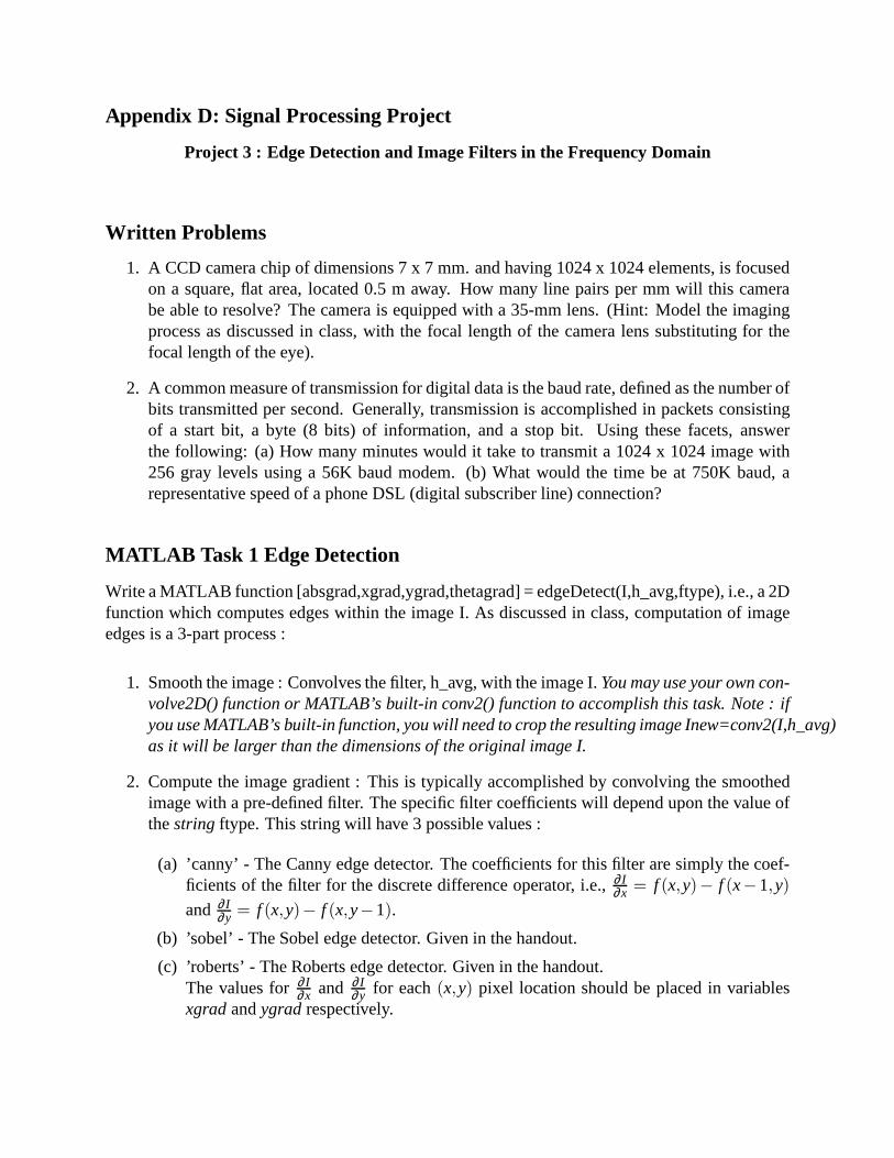
1. A CCD camera chip of dimensions 7 x 7 mm. and having 1024 x 1024 elements, is focusedon a square, flat area, located 0.5 m away. How many line pairs per mm will this camerabe able to resolve? The camera is equipped with a 35-mm lens. (Hint: Model the imagingprocess as discussed in class, with the focal length of the camera lens substituting for thefocal length of the eye).

2. A common measure of transmission for digital data is the baud rate, defined as the number ofbits transmitted per second. Generally, transmission is accomplished in packets consistingof a start bit, a byte (8 bits) of information, and a stop bit. Using these facets, answerthe following: (a) How many minutes would it take to transmita 1024 x 1024 image with256 gray levels using a 56K baud modem. (b) What would the timebe at 750K baud, arepresentative speed of a phone DSL (digital subscriber line) connection?

MATLAB Task 1 Edge Detection

Write a MATLAB function [absgrad,xgrad,ygrad,thetagrad]= edgeDetect(I,h_avg,ftype), i.e., a 2Dfunction which computes edges within the image I. As discussed in class, computation of imageedges is a 3-part process :

1. Smooth the image : Convolves the filter, h_avg, with the image I.You may use your own con-volve2D() function or MATLAB’s built-in conv2() function to accomplish this task. Note : ifyou use MATLAB’s built-in function, you will need to crop theresulting image Inew=conv2(I,h_avg)as it will be larger than the dimensions of the original imageI.

2. Compute the image gradient : This is typically accomplished by convolving the smoothedimage with a pre-defined filter. The specific filter coefficients will depend upon the value ofthestring ftype. This string will have 3 possible values :

(a) ’canny’ - The Canny edge detector. The coefficients for this filter are simply the coef-ficients of the filter for the discrete difference operator, i.e., ∂ I

∂x = f (x,y)− f (x−1,y)

and ∂ I∂y = f (x,y)− f (x,y−1).

(b) ’sobel’ - The Sobel edge detector. Given in the handout.

(c) ’roberts’ - The Roberts edge detector. Given in the handout.The values for∂ I

∂x and ∂ I∂y for each(x,y) pixel location should be placed in variables

xgradandygradrespectively.

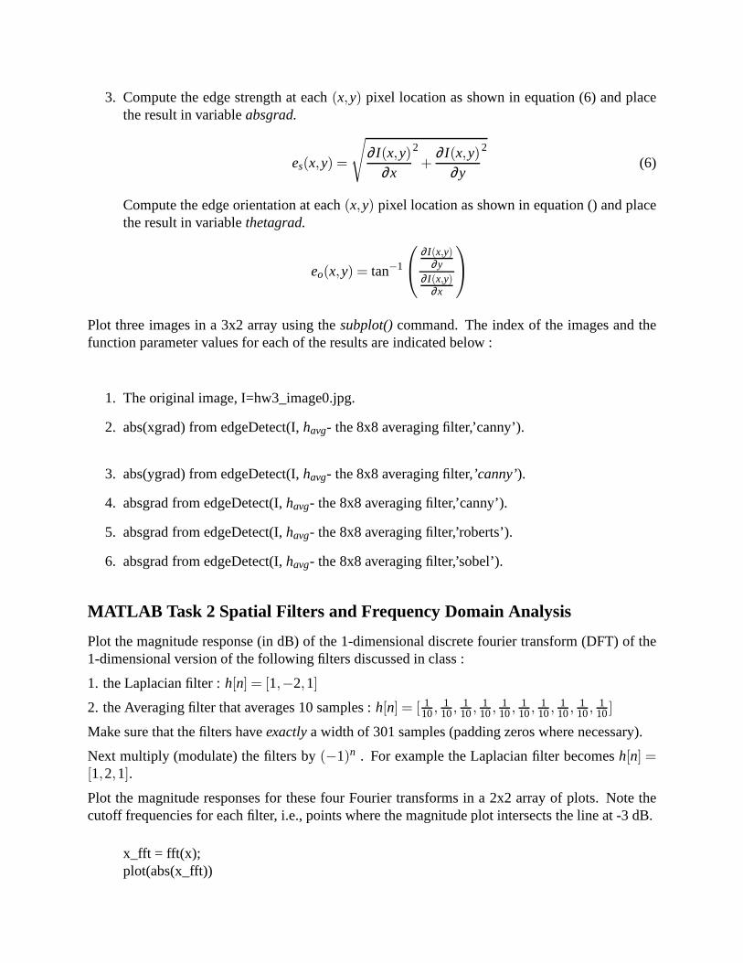
3. Compute the edge strength at each(x,y) pixel location as shown in equation (6) and placethe result in variableabsgrad.

es(x,y) =

√

∂ I(x,y)∂x

2

+∂ I(x,y)

∂y

2

(6)

Compute the edge orientation at each(x,y) pixel location as shown in equation () and placethe result in variablethetagrad.

eo(x,y) = tan−1

∂ I(x,y)∂y

∂ I(x,y)∂x

Plot three images in a 3x2 array using thesubplot()command. The index of the images and thefunction parameter values for each of the results are indicated below :

1. The original image, I=hw3_image0.jpg.

2. abs(xgrad) from edgeDetect(I,havg- the 8x8 averaging filter,’canny’).

3. abs(ygrad) from edgeDetect(I,havg- the 8x8 averaging filter,’canny’).

4. absgrad from edgeDetect(I,havg- the 8x8 averaging filter,’canny’).

5. absgrad from edgeDetect(I,havg- the 8x8 averaging filter,’roberts’).

6. absgrad from edgeDetect(I,havg- the 8x8 averaging filter,’sobel’).

MATLAB Task 2 Spatial Filters and Frequency Domain Analysis

Plot the magnitude response (in dB) of the 1-dimensional discrete fourier transform (DFT) of the1-dimensional version of the following filters discussed inclass :

1. the Laplacian filter :h[n] = [1,−2,1]

2. the Averaging filter that averages 10 samples :h[n] = [ 110,

110,

110,

110,

110,

110,

110,

110,

110,

110]

Make sure that the filters haveexactlya width of 301 samples (padding zeros where necessary).

Next multiply (modulate) the filters by(−1)n . For example the Laplacian filter becomesh[n] =[1,2,1].

Plot the magnitude responses for these four Fourier transforms in a 2x2 array of plots. Note thecutoff frequencies for each filter, i.e., points where the magnitude plot intersects the line at -3 dB.

x_fft = fft(x);plot(abs(x_fft))

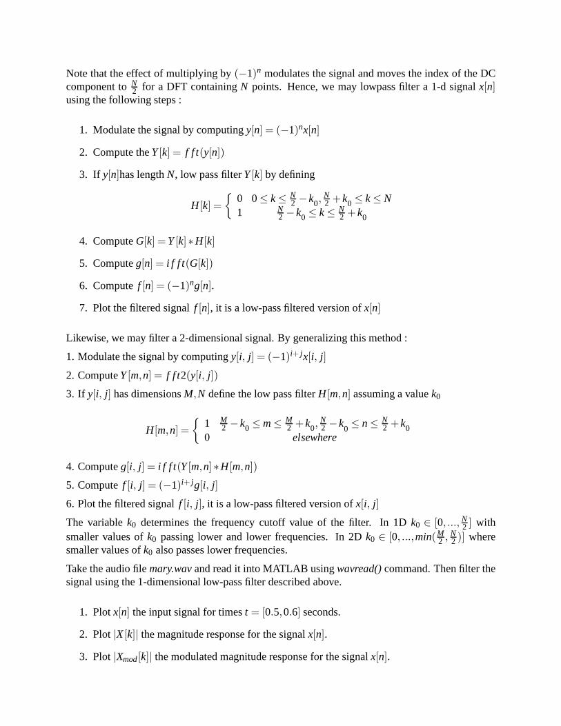
Note that the effect of multiplying by(−1)n modulates the signal and moves the index of the DCcomponent toN

2 for a DFT containingN points. Hence, we may lowpass filter a 1-d signalx[n]using the following steps :

1. Modulate the signal by computingy[n] = (−1)nx[n]

2. Compute theY[k] = f f t(y[n])

3. If y[n]has lengthN, low pass filterY[k] by defining

H[k] =

{

0 0≤ k≤ N2 −k0,

N2 +k0 ≤ k≤ N

1 N2 −k0 ≤ k≤ N

2 +k0

4. ComputeG[k] = Y[k]∗H[k]

5. Computeg[n] = i f f t (G[k])

6. Computef [n] = (−1)ng[n].

7. Plot the filtered signalf [n], it is a low-pass filtered version ofx[n]

Likewise, we may filter a 2-dimensional signal. By generalizing this method :

1. Modulate the signal by computingy[i, j] = (−1)i+ jx[i, j]

2. ComputeY[m,n] = f f t2(y[i, j])

3. If y[i, j] has dimensionsM,N define the low pass filterH[m,n] assuming a valuek0

H[m,n] =

{

1 M2 −k0 ≤ m≤ M

2 +k0,N2 −k

0≤ n≤ N

2 +k00 elsewhere

4. Computeg[i, j] = i f f t (Y[m,n]∗H[m,n])

5. Computef [i, j] = (−1)i+ jg[i, j]

6. Plot the filtered signalf [i, j], it is a low-pass filtered version ofx[i, j]

The variablek0 determines the frequency cutoff value of the filter. In 1Dk0 ∈ [0, ...,N2 ] with

smaller values ofk0 passing lower and lower frequencies. In 2Dk0 ∈ [0, ...,min(M2 ,

N2 )] where

smaller values ofk0 also passes lower frequencies.

Take the audio filemary.wavand read it into MATLAB usingwavread()command. Then filter thesignal using the 1-dimensional low-pass filter described above.

1. Plotx[n] the input signal for timest = [0.5,0.6] seconds.

2. Plot|X[k]| the magnitude response for the signalx[n].

3. Plot|Xmod[k]| the modulated magnitude response for the signalx[n].

4. Plot|H[k]| the magnitude response for the filter assumingk0 = 100.

5. Plot|X[k]H[k]| the magnitude response for the filtered signal.

6. Plotg[n] the filtered time domain signal.

Take the image filelena.gif and read it into MATLAB using theimread()command. Then filterthe image using the 2-dimensional low-pass filter describedabove.

1. PlotI [i, j] the input image.

2. Plot|X[i, j]| the magnitude response for the imageI [i, j].

3. Plot|Xmod[i, j]| the modulated magnitude response for the imageI [i, j].

4. Plot|H[i, j]| the magnitude response for the 2D filter assumingk0 = 80.

5. Plot|X[i, j]H[i, j]| the magnitude response for the filtered signal.

6. Plotg[i, j] the filtered image.

Completing your code and annotating your Results

Complete your MATLAB assignment by annotating your displayed results and commenting yourwritten MATLAB functions.

To Turn in :

1. Solutions to written problems.

2. Printouts of the MATLAB filesedgeDetect.m.

3. Printouts of your MATLAB filter programs for task 2.

4. Pages showing the annotated image plots for the requestedresults from tasks 1 and 2.

5. Two short paragraphs describing what you have learned / observed from completing each ofthe tasks.