Design of Thermoelectric Heat Pump for Active Building Envelope Systems Ritesh Khire Achille Messac Corresponding Author Achille Messac, Ph.D. Distinguished Professor and Department Chair Mechanical and Aerospace Engineering Syracuse University, 263 Link Hall Syracuse, New York 13244, USA Email: [email protected]Tel: (315) 443-2341 Fax: (315) 443-3099 https://messac.expressions.syr.edu/ Bibliographical Information Khire, R. A., and Messac, A., “Design of Thermoelectric Heat Pump for Active Building Envelope Systems,” 2005 ASME International Mechanical Engineering Congress and Exposition, IMECE2005-82490, Florida, Nov. 5-11, 2005.
Khire, R. A., and Messac, A., “Design of Thermoelectric Heat Pump for Active Building Envelope Systems,” 2005 ASME International Mechanical Engineering Congress and Exposition, IMECE2005-82490, Florida, Nov. 5-11, 2005.
International Journal of Heat and Mass Transfer 48 (2005) 4028–4040
www.elsevier.com/locate/ijhmt
Design of thermoelectric heat pump unit for activebuilding envelope systems
Ritesh A. Khire a, Achille Messac a,*, Steven Van Dessel b
a Department of Mechanical and Aerospace Engineering, Rensselaer Polytechnic Institute, Troy, NY 12180, United Statesb School of Architecture, Rensselaer Polytechnic Institute, Troy, NY 12180, United States
Received 25 June 2004; received in revised form 1 April 2005
Abstract
Active building envelope (ABE) systems represent a new thermal control technology that actively uses solar energyto compensate for passive heat losses or gains in building envelopes or other enclosures. This paper introduces initialsteps in exposing the community to this new technology, and explores an optimization based design strategy for its fea-sible application. We discuss the overall ABE system, and focus on the design and analysis of a key component—thethermoelectric heat pump unit, or the TE unit. This unit becomes an integral part of the generic enclosure, and is acollection of thermoelectric coolers, or heaters. As a critical component of the optimization based design strategy, com-putationally inexpensive approximate analytical models of generic TE coolers/heaters (referred to as TE coolers) aredeveloped. A multi-objective optimization technique is implemented to design and evaluate different design configura-tions of the TE unit. The multi-objective optimization simultaneously minimizes two design objectives: (1) the totalinput power required to operate the TE unit and (2) the number of TE coolers for economic considerations. Preliminaryresults indicate that the total input power required to operate the TE unit decreases as the distribution density of the TEcoolers increases. In addition, the thermal resistance of the heat sink (attached to the TE cooler) plays a key role indetermining the number of TE coolers required. These preliminary findings may have practical implications, influencingthe implementation of the ABE system.� 2005 Elsevier Ltd. All rights reserved.
Keywords: Active building envelope; Thermoelectric; Optimization; Heat sink; Air conditioning; Housing
1. Introduction
Active building envelope (ABE) systems represent anew thermal control technology that actively uses solarenergy to compensate for passive heat losses or gainsin building envelopes or other enclosures. In ABE sys-
0017-9310/$ - see front matter � 2005 Elsevier Ltd. All rights reservdoi:10.1016/j.ijheatmasstransfer.2005.04.028
tems, solar radiation energy is converted into electricalenergy by means of a photovoltaic unit (PV unit). Sub-sequently, this electrical energy is used to power a ther-moelectric heat pump unit (TE unit), which is acollection of thermoelectric coolers (heaters in winter).The TE unit allows the transport of heat through theABE wall. The PV and TE units are integrated withinthe ABE system enclosure. The TE unit can operate ina heating or a cooling mode, depending on the directionof the current supplied by the PV unit. This featureallows for the ABE system to be used for heating as
h natural convection coefficientk thermal conductivity of the thermoelectric
elementkhs thermal conductivity of the heat sinkmhs mass of the heat sinkn number of thermocouples per TE coolernf number of finstf thickness of the fintb thickness of the heat sink base platetABE the thickness of the ABE wallw1,w2 weights of the aggregate objective functionA area of cross-section of the thermoelectric
elementAABE surface area of the ABE wallAb area of the heat sink base plateAf cross-sectional area of the finAsc area of the heat source in contact with the
heat sinkCOP coefficient of performanceI input current supplied by the PV unitImax maximum allowable input currentK thermal conductance of the thermocoupleL length of the thermoelectric elementLcf corrected length of the finLf length of the finN number of thermoelectric coolersPf perimeter of the finPin input power supplied by the PV unitQhs heat dissipated through the heat sink
Qload heat dissipated by the heat sourceQpc heat absorbed at the cold end of the TE
coolerQph heat generated at the hot end of the TE
coolerR electrical resistance of the thermocoupleRb base spreading resistanceRf thermal resistance of the finsRhs thermal resistance of the heat sink
RTEth thermal resistance of the TE unit
S relative Seebeck coefficientTc temperature of the cold end of the TE coolerTh temperature of the hot end of the TE coolerTmax maximum allowable temperature for the TE
coolerTo ambient air temperatureV input voltage supplied by the PV unitVmax maximum allowable input voltage for the
TE coolerVs Seebeck voltageWf width of the fin
Greek symbols
q electrical resistivity of thermoelectric ele-ment
qhs density of the heat sinkk ratio of the area of cross-section to the
length of thermoelectric element
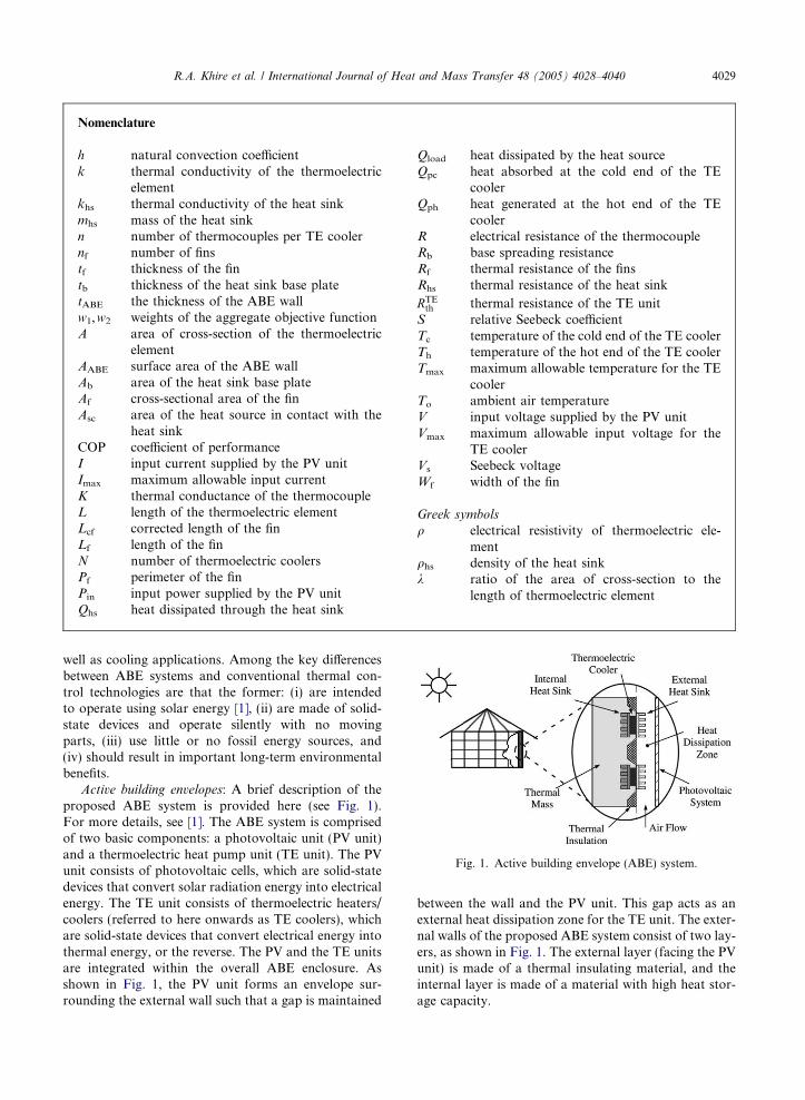
Fig. 1. Active building envelope (ABE) system.
R.A. Khire et al. / International Journal of Heat and Mass Transfer 48 (2005) 4028–4040 4029
well as cooling applications. Among the key differencesbetween ABE systems and conventional thermal con-trol technologies are that the former: (i) are intendedto operate using solar energy [1], (ii) are made of solid-state devices and operate silently with no movingparts, (iii) use little or no fossil energy sources, and(iv) should result in important long-term environmentalbenefits.
Active building envelopes: A brief description of theproposed ABE system is provided here (see Fig. 1).For more details, see [1]. The ABE system is comprisedof two basic components: a photovoltaic unit (PV unit)and a thermoelectric heat pump unit (TE unit). The PVunit consists of photovoltaic cells, which are solid-statedevices that convert solar radiation energy into electricalenergy. The TE unit consists of thermoelectric heaters/coolers (referred to here onwards as TE coolers), whichare solid-state devices that convert electrical energy intothermal energy, or the reverse. The PV and the TE unitsare integrated within the overall ABE enclosure. Asshown in Fig. 1, the PV unit forms an envelope sur-rounding the external wall such that a gap is maintained
between the wall and the PV unit. This gap acts as anexternal heat dissipation zone for the TE unit. The exter-nal walls of the proposed ABE system consist of two lay-ers, as shown in Fig. 1. The external layer (facing the PVunit) is made of a thermal insulating material, and theinternal layer is made of a material with high heat stor-age capacity.
Material 1 Material 2
Heat Released (Qph , Th)
Heat Absorbed (Qpc , Tc)
Cold Junction
Hot Junction
L
V
I
Fig. 2. Schematic of a thermocouple.
4030 R.A. Khire et al. / International Journal of Heat and Mass Transfer 48 (2005) 4028–4040
In Fig. 1, the words ‘‘Thermal insulation’’ and‘‘Thermal Mass’’ pertain to the external and the internallayers of the ABE wall, respectively. The TE coolers aredispersed inside the openings that are provided in theinsulating layer. Each TE cooler consists of two heatsinks. As shown in Fig. 1, the internal heat sink eitherabsorbs or dissipates heat to the thermal mass layer.The external heat sink either absorbs heat from, or dis-sipates heat to, the surrounding air; through natural orforced convection. In the present study, we have ne-glected the effect of the internal heat sink in keeping withthe scope of this preliminary study.
This paper is organized as follows. Section 2 de-scribes the approximate analytical models that are judi-ciously integrated in this study. Section 3 estimates thecooling load for a generic enclosure. Section 4 presentsthe optimization problem formulation for the design ofthe TE unit. The results are discussed in Section 5. Con-cluding remarks are provided in Section 6.
2. Basic models for ABE system
In the process of analyzing the overall ABE system,we first focus our attention on each unit in detail. In thispaper, we present the design and analysis of the TE unitfor the ABE system. Specifically, this section develops acomputationally inexpensive model of the TE unit.Here, the individual models of the components of theTE unit are coupled, yielding a single integrated modelthat takes into account the effect of the heat sink onthe TE cooler.
2.1. Thermoelectric cooler
This subsection describes the approximate analyticalmodel of a TE cooler. As shown in Fig. 2, when currentflows through the junction of two dissimilar conductors(also called a thermocouple), heat is either dissipated orabsorbed (depending on the direction of the current) atthat junction. This phenomenon is known as the Peltiereffect, and causes a decrease in the temperature at theheat-absorbing junction, and a simultaneous increasein the temperature at the heat-releasing junction [2–4].When current flows through a TE cooler that containsn thermocouples, the amount of heat absorbed at thecold junction (Qpc) is given by [5,6]
Qpc ¼ n SIT c � KðT h � T cÞ �1
2I2R
� �ð1Þ
where
K ¼ k1A1
L1
þ k2A2
L2
ð2Þ
R ¼ q1L1
A1
þ q2L2
A2
ð3Þ
In Eqs. (1)–(3), S is the relative Seebeck coefficient of thethermocouple; I is the input current flowing through thecircuit; Tc and Th are the temperatures of the cold andthe hot junctions, respectively; K is the thermal conduc-tance of the thermocouple; R is the electrical resistanceof the thermocouple; k is the thermal conductivity; q isthe electrical resistivity; and A and L represent thecross-sectional area and the length of the thermoelectricelement, respectively. The subscripts 1 and 2 refer to thethermoelectric materials 1 and 2, respectively.
2.2. Heat sink
Heat sinks lower or maintain the temperature of a de-vice by dissipating heat into the surrounding medium.The primary requirement of an effective heat sink is toprovide a low thermal resistance path for heat dissipa-tion. In ABE systems, heat sinks are required to dissi-pate the heat generated at the hot side of the TEcoolers. The performance characteristics of the TE cool-er (e.g., input power, heat absorption capacity) aregreatly affected by the thermal resistance of the associ-ated heat sink. Failure to dissipate the required heatfrom the TE cooler may result in an increase in its hotside temperature. As per Holman [7], the heat dissipatedby a heat sink is given by
Qhs ¼T h � T o
Rhs
ð4Þ
where Qhs is the heat dissipated by the heat sink, Th isthe temperature of the heat source (in the ABE systems,the hot end of the TE cooler), To is the ambient air tem-perature, and Rhs is the thermal resistance of the heatsink, given by
Rhs ¼ Rf þ Rb ð5Þ
Wf
Lf tf
Cross sectional area (Af)
Base plate
Fin
Pf
Base Plate
Thermoelectric Cooler
Fins To
Th
Rb
Rf
Qhs(a)
(b)
Fig. 3. Schematic of a heat sink: (a) thermal circuit of a heatsink and (b) geometric parameters of a fin.
R.A. Khire et al. / International Journal of Heat and Mass Transfer 48 (2005) 4028–4040 4031
where Rf and Rb represent the thermal resistances of thefins and the base (also called the base spreading resis-tance), respectively. Fig. 3(a) shows the thermal circuitof a heat sink. As shown in Fig. 3(a), the fin resistanceand the base spreading resistance are in series. The heatgenerated by the heat source (the hot side of the TEcooler) is conducted through the heat sink, which is thendissipated to the surrounding medium by convection.The following subsections present the approximate ana-lytical models for estimating the fin resistance and thebase spreading resistance of the heat sink.
2.2.1. Fin resistance
A typical heat sink consists of thin metal projections,called fins, as shown in Fig. 3(a). Fins provide additionalsurface area to increase the convection heat transfer.When a heat sink is exposed to natural convection, itis called a passive heat sink, and when it is exposed toforced convection, it is called an active heat sink [7].In the present study, we analyze a passive heat sink.Also, for the present study, we will consider an extrusiontype heat sink, which is suitable for low heat dissipationapplications such as ABE systems. The thermal resis-tance of a single fin heat sink is given by [7]
In Eqs. (6) and (7), h is the natural convection coeffi-cient; khs is the thermal conductivity of the heat sink;and Pf, Af, and Lcf are the perimeter, the area ofcross-section, and the corrected length of the fin, respec-tively. These quantities are evaluated as [7]
P f ¼ 2ðW f þ tfÞ ð8ÞAf ¼ W f � tf ð9ÞLcf ¼ Lf þ tf=2 ð10Þ
In Eqs. (8)–(10), the variablesWf, tf, and Lf represent thewidth, the thickness, and the length of the fin, respec-tively. The basic geometric parameters of a fin are illus-trated in Fig. 3(b). By multiplying Eq. (6) by the numberof fins (nf), we can estimate the fin resistance of a multi-ple fin heat sink.
We note that, in this paper, we approximate the heattransfer between the fin surfaces and the surrounding airusing the natural convection coefficient (h). This approxi-mation assumes that the air in contact with the fin sur-faces is maintained at the ambient air temperature (To),at all times. Such an approximation is in agreement withthe preliminary nature of this design study. However, infuture studies, a detailed analysis of the heat transferprocess at the fin surfaces is required, which takes intoaccount the effect of the localized increase in the air tem-perature on the natural convection process.
2.2.2. Base spreading resistance
The base spreading resistance needs to be consideredwhen a heat source with a smaller heat dissipation areais mounted over a heat sink with a larger base plate area[8], as shown in Fig. 3(a). This increases the base platetemperature at the location of the heat source. Thebase spreading resistance is given by the empirical for-mula [8]
In Eqs. (11) and (12), Ab is the area of the base plate ofthe heat sink; Asc is the area of the heat source, which isin contact with the base plate; and Ravg is the averagethermal resistance of the heat sink, which is assumedto be equal to the fin resistance, Rf, according to Ref.[9]. In the current paper, we assume the spacing betweenfins to be equal to the fin thickness. The area of the heatsink base plate is determined as Ab = (2nf � 1)tfwf.
2.3. Estimating the effect of heat sink on TE cooler
As stated in the previous subsection, a heat sink is re-quired to dissipate the heat generated at the hot junction
SUN
To Ti
ABE-wall (RABE)
Insulated walls (Rwall)
Qload
1 m
1 m
RABE << Rwall
Fig. 4. Generic enclosure containing single ABE wall.
4032 R.A. Khire et al. / International Journal of Heat and Mass Transfer 48 (2005) 4028–4040
of the TE cooler. The heat generated at the hot junctionof the TE cooler (Qph) is given by [10]
Qph ¼ Qpc þ VI ð13Þ
where V is the voltage across the TE unit. Since the heatsink is required to dissipate this heat, we haveQhs = Qph. Using Eqs. (4) and (13), we obtain an expres-sion for the temperature at the hot end of the TE cooleras [10]
T h ¼ T o þ ðQpc þ VIÞRhs ð14Þ
Substituting Eq. (14) into Eq. (1) to eliminate Th, we candetermine the effect of a heat sink on a TE cooler;namely, the dependence of Qpc on Rhs.
We conclude this section by commenting on themodel accuracy assessment work that we have per-formed. We have assessed the accuracies of the approx-imate analytical models described in this section bycomparing their results with those from more compre-hensive models developed in the literature, which wouldbe less suitable for the preliminary nature of our optimi-zation based design study. We used the model developedby Visser and de Kock [11] to assess the accuracy of theheat sink model, and the model developed by Nagy andBuist [10] to assess the accuracy of the model for esti-mating the effect of the heat sink on the TE cooler[12]. We observed that the difference between the resultsfrom the two models (approximate and comprehensive)is less than 15%, which is acceptable for this study.These comparative results lend sufficient credence tothe analytical models presented in this section, makingthem appropriate for the preliminary optimal design ofthe TE unit. Next, we evaluate different configurationsof the TE unit for a generic enclosure. In the next sec-tion, a cooling load is estimated for this enclosure undercertain assumed conditions.
3. Estimation of cooling load for a generic enclosure
To demonstrate the application of the proposed opti-mization based strategy to design the TE unit of theABE system, we analyze the model of a 1 m · 1 m ·1 m generic enclosure. This section provides the assump-tions made in this design study, and the estimation of thecooling load for this enclosure. Fig. 4 schematically rep-resents the generic enclosure for which the TE unit isdesigned.
3.1. Assumptions
The following assumptions are made for the genericenclosure. (1) The thickness of the ABE wall is tABE =0.15 m. (2) Only one of the four sidewalls acts as theABE wall, and heat losses or gains from the other side-walls are negligible. (3) The thermal conductivity of the
ABE wall is kABE = 0.05 W/m K. (4) The external tem-perature is To = 38 �C, and the internal temperature isTi = 20 �C. (5) The conduction heat transfer throughthe ABE wall is the only mode of heat transfer. (6) AllTE coolers in a TE unit absorb equal amount of heat,and the total heat absorption is uniform throughoutthe wall. (7) Each TE cooler has heat sinks capable ofabsorbing and releasing the required amount of heat.(8) All the TE coolers are connected in series. (9) Thetemperature of the cold end of the TE cooler is equalto the internal temperature (Tc = Ti). (10) The effect ofthe change in the external temperature, To, on the per-formance of the PV unit is neglected. (11) The effect ofair circulation on the overall heat transfer process isneglected.
3.2. Estimation of cooling load
Fig. 4 shows the top view of the generic enclosure(1 m · 1 m · 1 m), which is used to demonstrate theapplication of the proposed strategy for designing a gen-eric TE unit. We assume that the heat transfer from theexternal environment into the generic enclosure (or thereverse) is through the ABE wall only. The amount ofheat conducted through the ABE wall is given by Fou-rier�s law as
Qload ¼ kABEAABET o � T i
tABE
ð15Þ
where AABE is the surface area of the ABE wall. For thegeneric enclosure, AABE = 1 m · 1 m. Substituting theappropriate numerical values from Section 3.1, we ob-tain the heat gained by the enclosure through conduc-tion as 6 W.
Apart from the heat gained because of conduction, atypical room with 10 m2 floor area gains approximately
R.A. Khire et al. / International Journal of Heat and Mass Transfer 48 (2005) 4028–4040 4033
240 W of heat from the electrical appliances and thepeople in that room. For the generic enclosure, the floorarea is 1 m2 or 10% of the typical room described above.To account for the additional heat gained because of thefactors described above, we add 0.1 · 240 = 24 W to theheat gain. Thus the total heat gain is 6 + 24 = 30 W.This heat gain will act as the cooling load, Qload, forthe ABE system. To compensate this cooling load, weidentify the optimal configurations of the TE units.The next section describes the optimization based designstrategy for the TE unit.
4. Optimization based design strategy
This section describes the proposed strategy to designan appropriate configuration of the TE unit for the gen-eric enclosure described in the previous section. Thisstrategy involves the application of multi-objective opti-mization to obtain a preliminary conceptual design con-figuration of the TE unit. According to the previoussection, the estimated total cooling load for the genericenclosure is 30 W. Using multi-objective optimization,we determine the optimal number of TE coolers andthe appropriate heat sink geometry, to compensate theestimated cooling load. In this paper, we consider twodesign objectives: (1) electrical power required to oper-ate the TE unit, and (2) the number of TE coolers. Bothof the objectives are minimized simultaneously by com-bining them into a single aggregate objective function(AOF) [13]. The optimization problem involves a cou-pling between the performance of the TE cooler and thatof the heat sink. The following subsections describe thedesign variables, the design constraints, and the objec-tive function for formulating the optimization problem.
4.1. Design variables
The optimization problem involves seven design vari-ables, two for the TE cooler and five for the heat sink.The number of TE coolers (N) and the input current(I) are the two design variables for the TE cooler. Forthe heat sink, the five design variables are: the lengthof the fin (Lf), the width of the fin (Wf), the thickness ofthe fin (tf), the number of fins (nf), and the thickness ofthe base plate (tb). During the optimization process, thenumber of TE coolers is not allowed to become less thanone; and no upper limit is provided for the number ofTE coolers. The TE coolers are selected from theMelcor product catalog [14]. The input current (I) isnot allowed to exceed the maximum allowable current(Imax), which is specified in the Melcor product catalog.The upper and the lower bounds imposed on the remain-ing design variables are given in the optimization prob-lem statement (Eqs. (24)–(28)). (Note that the upper andlower bounds are in mm.)
4.2. Design constraints
The total heat absorbed by all the TE coolers is usedas an equality constraint in the optimization problem.Eq. (1) determines the amount of heat absorbed by a sin-gle TE cooler (Qpc). The total heat absorbed by all theTE coolers is calculated by multiplying the amount ofheat absorbed by a single TE cooler by the number ofTE coolers (N). During the optimization process, the to-tal heat absorbed by all the TE coolers is constrained toequal the estimated cooling load (Qload).
The temperature of the hot side of the TE cooler (Th)is used as the first inequality constraint in the optimiza-tion problem. Eq. (14) evaluates the temperature of thehot side of the TE cooler. This temperature is not al-lowed to exceed the maximum allowable temperaturefor the TE cooler (Tmax), which is specified in the Melcorproduct catalog [14].
The input voltage (V) applied to a single TE cooler isused as the second inequality constraint in the optimiza-tion problem. The input voltage for a single TE cooler isgiven by
V ¼ SðT h � T cÞ þ IR ð16Þ
This input voltage is not allowed to exceed the maxi-mum voltage (Vmax), which is specified in the Melcorproduct catalog [14]. For favorable numerical condi-tioning properties of the optimization process, allconstraints are normalized as shown in Eqs. (19)–(21).
4.3. Objective functions
4.3.1. Input power
The total electrical power (Pin) required to operate allthe TE coolers, is used as the first design objective andis given by
P in ¼ N � V � I ð17Þ
In ABE systems, the TE unit is powered by the PV unit(solar cells). There are several reasons why it is impera-tive that the input power, which is supplied by the PVunit, be minimized. The PV unit only produces electricalenergy during the part of the day when solar radiation isavailable [15]. The surface area available to place the PVunit on the ABE wall is limited. The limited availablesteady state solar power may not meet peak demand.As a result, there may be a need to store power for useat night and at peak power demand periods. Hence,minimizing the input power is central to the feasibilityof this system.
4.3.2. Number of TE coolers
We use the number of TE coolers (N) as the seconddesign objective in this paper. There are several
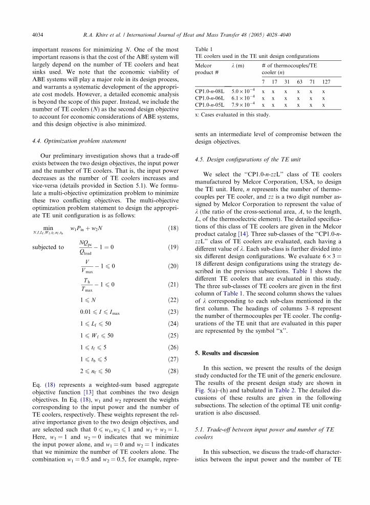
Table 1TE coolers used in the TE unit design configurations
Melcorproduct #
k (m) # of thermocouples/TEcooler (n)
7 17 31 63 71 127
CP1.0-n-08L 5.0 · 10�4 x x x x x xCP1.0-n-06L 6.1 · 10�4 x x x x x xCP1.0-n-05L 7.9 · 10�4 x x x x x x
x: Cases evaluated in this study.
4034 R.A. Khire et al. / International Journal of Heat and Mass Transfer 48 (2005) 4028–4040
important reasons for minimizing N. One of the mostimportant reasons is that the cost of the ABE system willlargely depend on the number of TE coolers and heatsinks used. We note that the economic viability ofABE systems will play a major role in its design process,and warrants a systematic development of the appropri-ate cost models. However, a detailed economic analysisis beyond the scope of this paper. Instead, we include thenumber of TE coolers (N) as the second design objectiveto account for economic considerations of ABE systems,and this design objective is also minimized.
4.4. Optimization problem statement
Our preliminary investigation shows that a trade-offexists between the two design objectives, the input powerand the number of TE coolers. That is, the input powerdecreases as the number of TE coolers increases andvice-versa (details provided in Section 5.1). We formu-late a multi-objective optimization problem to minimizethese two conflicting objectives. The multi-objectiveoptimization problem statement to design the appropri-ate TE unit configuration is as follows:
minN ;I ;Lf ;W f ;tf ;nf ;tb
w1P in þ w2N ð18Þ
subjected toNQpc
Qload
� 1 ¼ 0 ð19Þ
VV max
� 1 6 0 ð20Þ
T h
Tmax
� 1 6 0 ð21Þ
1 6 N ð22Þ
0.01 6 I 6 Imax ð23Þ
1 6 Lf 6 50 ð24Þ
1 6 W f 6 50 ð25Þ
1 6 tf 6 5 ð26Þ
1 6 tb 6 5 ð27Þ
2 6 nf 6 50 ð28Þ
Eq. (18) represents a weighted-sum based aggregateobjective function [13] that combines the two designobjectives. In Eq. (18), w1 and w2 represent the weightscorresponding to the input power and the number ofTE coolers, respectively. These weights represent the rel-ative importance given to the two design objectives, andare selected such that 0 6 w1,w2 6 1 and w1 + w2 = 1.Here, w1 = 1 and w2 = 0 indicates that we minimizethe input power alone, and w1 = 0 and w2 = 1 indicatesthat we minimize the number of TE coolers alone. Thecombination w1 = 0.5 and w2 = 0.5, for example, repre-
sents an intermediate level of compromise between thedesign objectives.
4.5. Design configurations of the TE unit
We select the ‘‘CP1.0-n-zzL’’ class of TE coolersmanufactured by Melcor Corporation, USA, to designthe TE unit. Here, n represents the number of thermo-couples per TE cooler, and zz is a two digit number as-signed by Melcor Corporation to represent the value ofk (the ratio of the cross-sectional area, A, to the length,L, of the thermoelectric element). The detailed specifica-tions of this class of TE coolers are given in the Melcorproduct catalog [14]. Three sub-classes of the ‘‘CP1.0-n-zzL’’ class of TE coolers are evaluated, each having adifferent value of k. Each sub-class is further divided intosix different design configurations. We evaluate 6 · 3 =18 different design configurations using the strategy de-scribed in the previous subsections. Table 1 shows thedifferent TE coolers that are evaluated in this study.The three sub-classes of TE coolers are given in the firstcolumn of Table 1. The second column shows the valuesof k corresponding to each sub-class mentioned in thefirst column. The headings of columns 3–8 representthe number of thermocouples per TE cooler. The config-urations of the TE unit that are evaluated in this paperare represented by the symbol ‘‘x’’.
5. Results and discussion
In this section, we present the results of the designstudy conducted for the TE unit of the generic enclosure.The results of the present design study are shown inFig. 5(a)–(h) and tabulated in Table 2. The detailed dis-cussions of these results are given in the followingsubsections. The selection of the optimal TE unit config-uration is also discussed.
5.1. Trade-off between input power and number of TE
coolers
In this subsection, we discuss the trade-off character-istics between the input power and the number of TE
Fig. 5. Optimization results for different design configurations: (a) trade-off curves, (b) number of TE coolers, (c) total input power,(d) input current for single TE cooler, (e) total input voltage, (f) heat sink resistance, (g) base spreading resistance, and (h) hot sidetemperature.
R.A. Khire et al. / International Journal of Heat and Mass Transfer 48 (2005) 4028–4040 4035
Table 2Optimal parameters for all TE unit configurations
4036 R.A. Khire et al. / International Journal of Heat and Mass Transfer 48 (2005) 4028–4040
coolers. Fig. 5(a) shows the trade-off curves for the threeTE coolers that are shown in the fourth column of Table1 (that is, TE coolers with n = 17). Each curve in Fig.5(a) corresponds to the specific value of k. To generatethese trade-off curves, we change the weights w1 andw2 (Eq. (18)) between 0 and 1 in 10 equal increments.On each curve shown in Fig. 5(a), the point to the ex-treme right represents the case, where w1 = 1 andw2 = 0 (minimizing the input power alone). Similarly,the point to the extreme left on each curve representsthe case, where w1 = 0 and w2 = 1 (minimizing the num-
ber of TE coolers alone). As expected, minimizing onlythe input power results in a large number of TE coolers(extreme right) and minimizing only the number of TEcoolers results in a large input power (extreme left).However, the case w1 = w2 = 0.5 optimizes both of thesedesign objectives simultaneously, with relatively evenimportance. We observed similar trade-off characteris-tics for all the values of n that are evaluated in this study.Based on these observations, we use w1 = 0.5 andw2 = 0.5 in Eq. (18) for the subsequent discussion. How-ever, different designer preferences can be specified with
R.A. Khire et al. / International Journal of Heat and Mass Transfer 48 (2005) 4028–4040 4037
respect to the two design objectives by simply selectingan appropriate set of weights.
From Fig. 5(a), we observe that the TE cooler withk = 7.9 · 10�4 m results in the minimum objective func-tion values compared to the other two values of k. Weobserved similar behavior for all values of n consideredin this study. Hence, TE coolers with k = 7.9 · 10�4 m(‘‘CP1.0-n-05L’’ class) are assumed preferred over theother two classes.
In the following subsections, we discuss the effect ofimportant parameters on the performance of the TEunit. Also, we select the number of thermocouples, n,for the ‘‘CP1.0-n-05L’’ class of TE coolers, that offersthe optimal TE unit configuration. We note that inFig. 5(b)–(h), the horizontal axis represents n.
5.2. Number of thermoelectric coolers
The number of TE coolers is one of the design objec-tives used in this paper. In Fig. 5(b), the x-axis shows thenumber of thermocouples per TE cooler (n), and the y-axis shows the number of TE coolers (N) required tocompensate the estimated cooling load. As the numberof thermocouples per TE cooler, n, increases, the num-ber of TE coolers, N, required to compensate the esti-mated cooling load decreases. This relationship is inagreement with our expectations. However, the relationbetween the total number of TE coolers, N, and thenumber of thermocouples per TE cooler, n, is not lin-ear. The explanation for this behavior is given in Section5.7. From Fig. 5(b), We can also observe that the num-ber of TE coolers is not significantly affected by thevalue of k.
Although we minimize the number of TE coolers inthe optimization formulation, we note that for a TE unitconfiguration with a small number of TE coolers (lessthan 10), the heat absorption across the ABE wall maynot be uniform. This will violate one of the assumptionsmade in this study (Assumption 6 in Section 3.1). Inother words, the approximate analytical model will notadequately predict the actual behavior of the TE unitfor the generic enclosure.
Based on the above discussion, some of the TE cool-ers from the preferred ‘‘CP1.0-n-05L’’ class become lessdesirable, as they result in N < 10. In Fig. 5(b), the TEunit configurations marked A, B, and C have N P 10and are expected to ensure relatively uniform heatabsorption across the ABE wall. Hence, these three TEunit configurations are preferred over the other TE unitconfigurations. Configurations A, B, and C requireapproximately 45 TE coolers of CP1.0-7-05L type, 20TE coolers of CP1.0-17-05L type, and 10 TE coolersof CP1.0-31-05L type, respectively. We will select oneof these configurations as the most preferred designbased on the second design objective, the input power,which is discussed next.
5.3. Total input power
The total input power is the second design objectiveused in this paper. Fig. 5(c) shows the total input power,Pin, for each of the configurations evaluated in thisstudy. The x-axis shows the number of thermocouplesper TE cooler, and the y-axis depicts the input power.As the number of thermocouples per TE cooler in-creases, so does the total input power. From Fig. 5(b),the number of TE coolers required to compensate thecooling load decreases as the number of thermocouplesper TE cooler increases. We can then observe that asthe distribution density of the TE coolers increases, thetotal input power required to operate the ABE systemdecreases, for the TE unit configurations evaluated inthis study. There would reach a point where this conclu-sion goes beyond practical and economic implementa-tion feasibility.
To identify the most appropriate configuration, wemake the following observations. From Fig. 5(c), theTE unit configurations A, B, and C require relativelylower input power than the other configurations. Hence,these three configurations are chosen as the preferredones, among the various TE unit configurations evalu-ated in this study. From Fig. 5(c), the preferred TE unitconfiguration A requires the lowest input power, fol-lowed by the configurations B and C, in that order.
Although the preferred configuration A requires thelowest input power among the three, it requires a largenumber of TE coolers (see Fig. 5(b)). An oppositebehavior can be observed for the preferred configurationC. However, the configuration B offers a balance be-tween the number of TE coolers and the input power,compared to the other two configurations. Hence, basedon the two design objectives used in this paper, we selectthe TE unit configuration B as the most preferred designconfiguration. This TE unit configuration consists of 20TE coolers of CP1.0-17-05L type, and requires approx-imately 19.6 W of input power (Fig. 5(c)), which needsto be supplied by the PV unit. The details of the mostpreferred configuration B are shown in bold letters inTable 2.
It is important to note that the results of the presentstudy may be improved by taking into account otherimportant practical considerations, such as the thermalcapacity of the ABE wall, and the effect of air circulationon the overall heat transfer process. In the followingsubsections, we discuss the effect of other importantparameters on the performance of the TE unit in gen-eral, and on that of configuration B in particular.
5.4. Input current
The input current required to operate a TE cooler ineach configuration of the TE unit is shown in Fig. 5(d).The x-axis shows the number of thermocouples per TE
4038 R.A. Khire et al. / International Journal of Heat and Mass Transfer 48 (2005) 4028–4040
cooler, and the y-axis shows the input current. The inputcurrent decreases as the number of thermocouples perTE cooler increases. However, this decrease in the inputcurrent is less than 1%, for the range of design configu-rations evaluated in this study. As stated in the assump-tions (Section 3.1), the TE coolers are connected in seriesand therefore the same current flows through all ofthem. Hence, every configuration of the TE unit will re-quire the same input current as shown in Fig. 5(d). It isimportant to note that the relationship between the in-put current and the number of thermocouples per TEcooler is not perfectly linear, as is seen in Fig. 5(d).The nonlinearities in the modeling equations, and thecoupling between the TE cooler and the heat sink are ex-pected to cause this behavior. A comprehensive exami-nation of this behavior of the input current is beyondthe scope of this paper.
The TE unit configuration B requires 1.4 A of inputcurrent. The PV unit, which comprises solar cells, is ex-pected to supply this input current. It may not be feasi-ble for a single solar cell to produce 1.4 A of current. Insuch a case, multiple solar cells connected in a parallelcircuit can be used to generate the required input cur-rent. We note that, in the present paper, we have notused the input current as a design objective in keepingwith the scope of this study. However, the input currentmay assume significance, especially in the regions whereample sunlight is not available, as the current generatedby the PV unit is proportional to the intensity of theincident solar radiation [15]. Next, we examine the volt-age across the TE unit, which expectedly has a lesserimpact on the selection process.
5.5. Input voltage across the TE unit
Fig. 5(e) shows the input voltage across the TE unitfor each design configuration. The x-axis and the y-axisrepresent the number of thermocouples per TE coolerand the input voltage, respectively. Since TE coolersare connected in series, the input voltage across the TEunit is the product of the input voltage per TE cooler,V, (Table 2) and the number of TE coolers, N. The inputvoltage across the TE unit increases linearly with thenumber of thermocouples per TE cooler. Since the PVunit can be treated as a current source, the input voltageacross the TE unit will have little impact on the selectionof the TE unit configuration.
According to Eq. (16), the input voltage is the sum oftwo components. The first is the product of the inputcurrent, I, and the electrical resistance, R; and is there-fore an explicit function of the input current. The secondis the Seebeck voltage, which is given by
V s ¼ SðT h � T cÞ ð29Þ
According to Eq. (14), for a given heat sink resistance,Rhs, the hot side temperature is an implicit function of
the input current. Hence, we deduce that the input volt-age for the TE unit is a function of the input current,and will have little impact on the selection of the TE unitconfiguration. However, the input voltage across the TEunit is one of the factors for consideration in the selec-tion of the PV unit. (Note that the design of the PV unitis not a part of the present study.) For the preferred con-figuration B, the total input voltage across the TE unit is14.1 V (see Fig. 5(e)).
The input voltage per TE cooler is used as one of theconstraints in the optimization problem. It is useful tonote that the input voltage per TE cooler was not anactive constraint for any design configuration. For allof the design configurations, the input voltage per TEcooler was always less than one-third of the maximuminput voltage (Vmax) [14]. Hence, in future analyses,which may involve combining the models of the PV unit,the inclusion of the voltage constraint may not provecritical.
5.6. Coefficient of performance
Coefficient of performance (COP) [7] is a measure ofthe efficiency of the TE unit and is evaluated as
COP ¼ Heat absorbed
Input power¼ Qload
P in
ð30Þ
The COP values for all of the design configurations aregiven in Table 2. Since the same cooling load is appliedto all design configurations (Qload = 30 W), the COP isinversely proportional to the total input power, as evalu-ated in Section 5.3. Hence, the plot of the COP versus thenumber of thermocouples per TE cooler would show in-verse trends compared to those in Fig. 5(c). For the pre-ferred configuration B, the COP is 1.529 (see Table 2).
5.7. Thermal resistance of the heat sink
Here we explain how the thermal resistance of theheat sink and the total number of TE coolers decreaseas the number of thermocouples per TE cooler increases.These observations represent the likely trends in theproperties of optimal ABE systems.
For each configuration of the TE unit, the thermalresistance of the heat sink is shown in Fig. 5(f). The x-axis and the y-axis represent the number of thermocou-ples per TE cooler and the thermal resistance of the heatsink, respectively. The required thermal resistance of theheat sink decreases rapidly as the number of thermocou-ples per TE cooler increases. According to Fig. 5(b)(Section 5.2), the relation between the number of TEcoolers and the number of thermocouples per TE cooleris also nonlinear. The various nonlinearities lead to somenotable observations. As the number of thermocouplesper TE cooler increases, each TE cooler compensates ahigher fraction of the estimated cooling load. This
R.A. Khire et al. / International Journal of Heat and Mass Transfer 48 (2005) 4028–4040 4039
behavior occurs because the resulting thermal resistanceof the heat sink rapidly decreases with the number ofthermocouples per TE cooler (see Fig. 5(f)). The presentbehavior of the thermal resistance of the heat sink isexamined next.
From Eq. (5), the thermal resistance of the heat sink,Rhs, is the sum of the fin resistance, Rf, and the basespreading resistance, Rb. According to Eq. (6), the finresistance depends on the geometric parameters andthe material properties of the heat sink. The latter are as-sumed to remain constant in this study. All the geomet-ric parameters of the heat sink (i.e. Lf, Wf, tf, nf, and tb)are made design variables in the optimization formula-tion. The results from Table 2 indicate that the heat sinkdesign converges to the same optimal geometry for allthe configurations. Hence, the values of the fin resis-tance, Rf, are equal for all design configurations evalu-ated in this study.
However, the base spreading resistance, Rb, of theheat sink behaves differently. As the number of thermo-couples per TE cooler increases, the area of the TEcooler, Asc, also increases [14]. Since the optimal geom-etry of the heat sink is independent of the TE cooler con-figuration, the base area of the heat sink, Ab, is constantfor all the design configurations evaluated in this study,and is equal to Ab = (2nf � 1)tfwf = 4950 mm2. For aconstant base area, the base spreading resistance, Rb,of the heat sink decreases as the TE cooler area increases(Eq. (11)). Fig. 5(g) shows the base spreading resistancefor each design configuration evaluated in this study. Weobserve that the base spreading resistance decreasesrapidly as the number of thermocouples per TE coolerincreases (Fig. 5(g)). Because of this decrease in the basespreading resistance, the total heat sink resistance, Rhs,decreases as the number of thermocouples per TE coolerincreases (Fig. 5(f)), and is not constant—as was the finresistance Rf.
As stated in Section 2.2, the primary requirement of aheat sink is to provide a low thermal resistance path forheat dissipation. From Fig. 5(f), the design configura-tions with 127 thermocouples per TE cooler have heatsinks with the least thermal resistance. However, thisobservation does not imply that these configurationshave superior heat dissipation capabilities. In the ther-
mal circuit of the TE unit, the heat sinks are parallelto each other. The thermal resistance of the completeTE unit, RTE
th , is determined by dividing the thermal resis-tance of a single heat sink, Rhs, by the number of heatsinks, N. The thermal resistances of the TE units areshown in Table 2. We can observe that the design config-urations with seven thermocouples per TE cooler resultsin the lowest RTE
th values, and those with 127 thermocou-ples per TE cooler results in the highest RTE
th values, forall of the values of k. We can also observe that the ther-mal resistance of the TE unit decreases with the numberof thermocouples per TE cooler.
However, it is important to note that through theoptimization process, appropriate heat sinks havebeen designed for all the TE unit configurations todissipate the entire heat generated at the hot junctionof the TE coolers (Qph). Interestingly, the thermal resis-tance of the heat sink is not the primary criterion forselecting the TE unit configuration for the genericenclosure.
5.8. Hot side temperature
We conclude this section by explaining how the hotside temperature of the TE cooler is not a significantdriving factor in the selection of the TE coolersconfiguration.
Fig. 5(h) depicts the hot side temperature of the TEcooler (Th) for each of the design configurations. Thehot side temperature is plotted against the number ofthermocouples per TE cooler. We observe that the hotside temperature increases with the number of thermo-couples per TE cooler. In the previous section we notedthat each TE cooler compensates a higher fraction of thecooling load as the number of thermocouples per TEcooler increases. This situation leads to an accompany-ing increase in the hot side temperature of the TE cooler.Appropriate heat sinks are then designed to dissipate therequired heat. Further, the hot side temperature of theTE cooler is much lower than the maximum allowabletemperature, Tmax [14]. Hence, the hot side temperatureof the TE cooler is not likely to be the primary criterionfor selecting the appropriate design configuration of theTE unit.
6. Conclusions
A multi-objective optimization based design strategywas proposed to design the thermoelectric unit (TE unit)of ABE systems. The application of the proposed designstrategy was demonstrated by designing a TE unit for ageneric enclosure. Computationally favorable approxi-mate analytical models of the TE cooler and heat sinkwere developed for a preliminary optimization study.The cooling load was estimated for a generic enclosure.The developed optimization approach was implementedto evaluate 18 different design configurations of the TEunit. The results indicate that the total input powerrequired to operate the TE unit decreases as the distribu-tion density of the TE coolers increases. It was observedthat the thermal resistance of the heat sink plays a keyrole in determining the optimal number of TE coolersin all of the design configurations. Based on the assump-tions made in the study, the TE unit configurationinvolving 20 TE coolers of CP1.0-17-05L type was foundto be optimal for the generic enclosure. This design rep-resents a trade-off between the input power requirement
4040 R.A. Khire et al. / International Journal of Heat and Mass Transfer 48 (2005) 4028–4040
and the number of TE coolers used in the TE unit. How-ever, the multi-objective nature of the formulation al-lows the incorporation of different designer preferenceswith respect to these objectives. This paper representsthe first step in the development of a design and analysisapproach for the practical implementation of ABEsystems.
Acknowledgements
Support from the National Science Foundation,award number CMS—0333568, Directorate for Engi-neering, Division of Civil and Mechanical Systems,and the US Department for Housing and Urban Devel-opment is much appreciated.
References
[1] S. Van Dessel, A. Messac, R. Khire, Active buildingenvelopes: a preliminary analysis, in: Asia InternationalRenewable Energy Conference, Beijing, China, 2004.
[2] D.D. Pollock, Thermocouples: Theory and Practice,CRC Press Inc., Boca Raton, FL, 1991, ISBN 0-8493-4243-0.
[4] D.M. Rowe, CRC Handbook of Thermoelectrics, IEEE,CRC Press, 1995, ISBN 0-8493-0146-7.
[5] J.R. Baird, D.F. Fletcher, B.S. Haynes, Local condensa-tion heat transfer rates in fine passages, Int. J. Heat MassTransfer 46 (23) (2003) 4453–4466.
[6] W. Seifert, M. Ueltzen, E. Muller, One-dimensionalmodeling of thermoelectric cooling, Phys. Stat. Sol. (a)194 (1) (2002) 277–290.
[8] S. Lee, Calculating spreading resistance in heat sinks,Electron. Cooling 4 (1) (1998) 30–33.
[9] Enertron Inc., Optimization of heat sink design and fanselection in portable electronics environment, ResearchArticle available on the official website of Enertron Inc.,April 2004.
[10] M.J. Nagy, R. Buist, Effect of heat sink design onthermoelectric cooling performance, AIP Conf. Proc. 316(1) (1994) 147–149.
[11] J.A. Visser, D.J. de Kock, Optimization of heat sink massusing the DYNAMIC-Q numerical optimization method,Commun. Numer. Methods Eng. 18 (10) (2002) 721–727.
[12] R. Khire, S. Van Dessel, A. Messac, Active buildingenvelopes: a new solar driven heat transfer mechanism, in:19th European PV Solar Energy Conference, Paris,France, 2004.
[13] A. Messac, A. Ismail-Yahaya, Required relationshipbetween objective function and Pareto frontier orders:Practical implications, AIAA J. 39 (11) (2001) 2168–2174.
[14] Melcor Corporation, Melcor Thermal Solutions Catalog,2004, pp. 47–49. Available from: <www.melcor.com>.
[15] M.A. Green, Solar Cells: Operating Principles, Technol-ogy, and System Application, Prentice-Hall, Inc., Engle-wood Cliff, NJ, 1982, ISBN 0-13-822270-3.