Design Options for Offshore Pipelines in the US Beaufort and Chukchi Seas Report R-07-078-519 MMS Contract M-07-PC-13015 Prepared for: US Department of the Interior Minerals Management Service April 2008 Captain Robert A. Bartlett Building Morrissey Road St. John’s, NL Canada A1B 3X5 T: (709) 737-8354 F: (709) 737-4706 [email protected]www.c-core.ca
Transcript
Design Options for Offshore Pipelines in the US Beaufort and
Chukchi Seas
Report R-07-078-519
MMS Contract M-07-PC-13015
Prepared for:
US Department of the Interior Minerals Management Service
April 2008
Captain Robert A. Bartlett Building Morrissey Road
Captain Robert A. Bartlett Building Morrissey Road St. John's, NL Canada A1B 3X5 T: (709) 737-8354 F: (709) 737-4706 [email protected] www.c-core.ca
Prepared for: US Department of the Interior Minerals Management Service
Prepared by: C-CORE Report R-07-078-519
MMS Contract M-07-PC-13015
April 2008
The correct citation for this report is: C-CORE (2008). Design Options for Offshore Pipelines in the US Beaufort and Chukchi Seas, C-CORE Report R-07-078-519v2.0, April 2008. Project Team Vincent Morgan – C-CORE (Project Manager) Brad Elliott – C-CORE David Tucker – C-CORE John Barrett – C-CORE Tony King – C-CORE Andrew Palmer – Bold Island Engineering Mike Paulin – IMVPA Jonathan Caines – IMVPA Shawn Kenny – Memorial University of Newfoundland
Design Options for Offshore Pipelines in the US Beaufort and Chukchi Seas US Department of the Interior, Minerals Management Service
Report R-07-078-519v2.0 April 2008
i
REVISION HISTORY VERSION SVN # NAME COMPANY DATE OF
CHANGES COMMENTS
1.0 V. Morgan C-CORE March 08 Draft Final Report
2.0 R. Phillips C-CORE April 08 MMS comments
incorporated
DISTRIBUTION LIST
COMPANY NAME NUMBER OF COPIES MMS Jim Lusher / Mik Else .pdf
Design Options for Offshore Pipelines in the US Beaufort and Chukchi Seas US Department of the Interior, Minerals Management Service
Report R-07-078-519v2.0 April 2008
i
EXECUTIVE SUMMARY
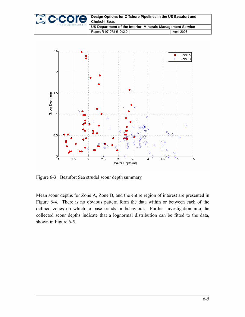
A detailed review of design issues relating to Arctic offshore pipelines for protection from ice gouging, strudel scour and upheaval buckling has been performed. The report presents interpretation of seabed survey data, analysis methods for pipeline response and demonstration of design methodologies for pipeline burial depth design. The study is focused on the US Beaufort and Chukchi Seas. Ice gouge data from surveys performed in the Beaufort and Chukchi Seas by the US Geological Survey in the 1970s and 1980s, and surveys related to the Northstar and Liberty Field developments have been reviewed and processed to provide a statistical representation of gouge geometry (depth and width) and crossing frequency. Consideration has been given to the survey limitations in terms of gouge cut-off depth, differentiation of single and multiplet gouges, potential sediment infill rates, dating of gouges through repetitive mapping and extrapolation of design parameters beyond data availability. Probability of exceedance curves for gouge depth, width and crossing density or frequency have been developed based on the available data for input into a probabilistic design process. Strudel scour seabed survey data related to the Northstar and Liberty Field developments have been reviewed to develop statistical representation of strudel scour depth, diameter and formation density. Exceedance curves have been developed in a similar manner to ice gouging. Issues relating to greater uncertainty due to a less comprehensive data source have been noted. Methods of analysis for the assessment of pipeline behaviour as a result of ice gouging or strudel scour action have been presented. Discussion of the available models for calculating soil displacements, pipeline structural behaviour and definition of failure criteria provides a framework for a probabilistic approach to pipeline design. Assessment of upheaval buckling potential, in combination with ice gouging is also discussed. Probabilistic assessments of pipeline burial depth requirements for protection from ice gouging and strudel scour have been presented based on an example pipeline route and design parameters. The examples demonstrate an approach that uses the survey data interpretation and analytical methods discussed through the report. The examples suggest that ice gouging presents an important design challenge, with significant burial depths
Design Options for Offshore Pipelines in the US Beaufort and Chukchi Seas US Department of the Interior, Minerals Management Service
Report R-07-078-519v2.0 April 2008
ii
being required. Strudel scour seems to be a less onerous condition based on interpretation of the available data. A brief discussion of construction, maintenance and repair of pipelines in Arctic conditions is provided for completeness. This aspect of project development is particularly important to provide the required confidence that systems can be designed, built and operated safely. A detailed assessment was outside the focus of this study. The following conclusions and recommendations are made as a result of this study: Ice Gouging
• Ice gouging is an important condition that must be considered as part of the offshore design process. Predicted burial depth requirements using currently available data and analysis methods can be significant and can control design conditions.
• There is a need for significantly increased regional coverage of repetitive mapping of the US Beaufort and Chukchi Seas to provide improved parameters of ice gouge geometry and crossing rates. Experience in the Canadian Beaufort Sea, where annual government funded surveys have taken place over the past 10 years or more, suggests that many years of data are needed to adequately provide statistical parameters for design. Consideration of infilling and erosion of gouges between formation and surveying must be considered.
• A consistent approach to reporting of gouge parameters, such as the differentiation of single and multiplet gouges and disturbed width should be developed to remove uncertainty in its interpretation.
• The statistical interpretation of gouge geometry to account for long return periods currently requires significant extrapolation beyond the available data. A greater quantity of survey data would reduce the need to extrapolate, but recognition of physical boundaries of the gouging process is required to establish gouge criteria that results in safe and economical designs.
• Current methodologies for the analysis of pipeline response to ice gouging predict significant burial depth requirements for the conditions experienced in the Beaufort and Chukchi Seas. Efforts are ongoing by a number of researchers to improve the level of understanding of ice gouging processes and develop the
Design Options for Offshore Pipelines in the US Beaufort and Chukchi Seas US Department of the Interior, Minerals Management Service
Report R-07-078-519v2.0 April 2008
iii
models that feed into burial depth design requirements. This is expected to improve the efficiency and lead to reduced cost for future projects in this region.
Strudel Scour
• The risk of strudel scour to pipelines does not seem to be significant based on the data and conditions reviewed.
• There is a small amount of data available for defining the risk to a pipeline, although efforts are ongoing to define areas where this process is expected to occur. Additional data will be required to define strudel scour geometry and formation density.
• Simple analytical methods can be developed to allow pipeline behaviour to be predicted when spanning a strudel scour. This is expected to be sufficient for preliminary design and for determining if this condition has a large impact on burial depth. More detailed modeling may be warranted where the risk of strudel scour may dominate the design condition.
Pipeline Buckling
• Upheaval and lateral pipeline buckling are considerations for all pipelines.
Accepted routine design methods have been developed to predict the onset of this behaviour. Arctic conditions have the potential to increase the severity of buckling due to increased temperature differentials between installation and operation.
• The interaction of buckling behaviour with ice gouging or strudel scour should be considered, and existing design methods may be modified to allow such checks to be performed.
Design Options for Offshore Pipelines in the US Beaufort and Chukchi Seas US Department of the Interior, Minerals Management Service
10 ARCTIC OFFSHORE PIPELINE CONSTRUCTABILITY, OPERATION, MAINTENANCE AND REPAIR............................................................................... 10-1
10.1 Construction.................................................................................................... 10-1 10.1.1 Winter Construction versus Open Water Construction ......................... 10-1 10.1.2 Permafrost and Trenchability................................................................. 10-2 10.1.3 Trenching Equipment............................................................................. 10-2 10.1.4 Pipeline Installation ............................................................................... 10-4 10.1.5 Trenching and Backfill .......................................................................... 10-7
10.2 Pipeline Inspection and Maintenance ............................................................. 10-8 10.2.1 Operations .............................................................................................. 10-8 10.2.2 Monitoring and Maintenance................................................................. 10-9
APPENDIX A Review of Existing Ice Gouge Data from the Beaufort Sea,
Alaska APPENDIX B Review of Existing Ice Gouge Data from the Eastern Chukchi
Sea, Alaska
Appendices supplied under separate cover.
Design Options for Offshore Pipelines in the US Beaufort and Chukchi Seas US Department of the Interior, Minerals Management Service
Report R-07-078-519v2.0 April 2008
vii
LIST OF TABLES
Table 2-1: Summary of borehole soil samples (Miller & Bruggers, 1980) .................... 2-9 Table 4-1: Frequency of New Gouges in Canadian Beaufort (Nessim and Hong, 1992)4-1 Table 4-2: Environmental parameters for Beaufort Sea case study zones...................... 4-4 Table 4-3: Summary of Rearic and McHendrie (1983) and Weber et al. (1989) data sets
.................................................................................................................................. 4-9 Table 4-4: Summary of MMS (2002) data sets ............................................................ 4-10 Table 4-5: Summary of Rearic and McHendrie (1983) Gouge Depths ........................ 4-19 Table 4-6: Single Gouge Depths (Weber et al., 1989).................................................. 4-23 Table 4-7: Multiplet Gouge Depths (Weber et al., 1989) ............................................. 4-23 Table 4-8: Summary of MMS (2002) gouge depths..................................................... 4-26 Table 4-9: Single gouge widths (Weber et al., 1989) ................................................... 4-34 Table 4-10: Multiplet gouge widths (Weber et al.,1989).............................................. 4-34 Table 4-11: Summary of MMS (2002) gouge widths................................................... 4-37 Table 4-12: Summary of Rearic and McHendrie (1983) gouge crossing density ........ 4-43 Table 4-13: Summary of Weber et al. (1989) gouge crossing density ......................... 4-47 Table 4-14: Summary of Weber et al. (1989) gouge crossing frequencies .................. 4-51 Table 5-1: Environmental parameters for Chukchi Sea case study zones ...................... 5-2 Table 5-2: Summary of data set used in study................................................................ 5-5 Table 5-3: Chukchi Sea geophysical surveys ................................................................. 5-6 Table 5-4: Summary of Toimil (1978) gouge depths ................................................... 5-13 Table 5-5: Summary of Toimil (1978) gouge depths ................................................... 5-16 Table 5-6: Summary of Toimil (1978) Gouge Density ................................................ 5-19 Table 6-1: Summary of strudel scour data set (MMS, 2002) ......................................... 6-2 Table 6-2: Summary of strudel scours ............................................................................ 6-3 Table 9-1: Beaufort Sea burial criteria............................................................................ 9-5 Table 9-2: Pipeline analysis base-case parameters ......................................................... 9-6 Table 9-3: Beaufort Sea burial criteria.......................................................................... 9-22
Design Options for Offshore Pipelines in the US Beaufort and Chukchi Seas US Department of the Interior, Minerals Management Service
Report R-07-078-519v2.0 April 2008
viii
LIST OF FIGURES
Figure 1-1: Schematic of gouging ice ridge keel ............................................................. 1-2 Figure 1-2: Strudel scour process .................................................................................... 1-5 Figure 1-3: Strudel scour investigated by direct diving observations (Reimnitz et al.,
1974) ........................................................................................................................ 1-6 Figure 1-4: Upheaval buckling of pipeline at overbend .................................................. 1-9 Figure 1-5: Example of upheaval buckling.................................................................... 1-10 Figure 1-6: Example of onshore lateral buckling .......................................................... 1-10 Figure 1-7: Example of offshore lateral buckling.......................................................... 1-11 Figure 2-1: Alaskan Beaufort Sea plan and bathymetry (MMS, 2002).......................... 2-2 Figure 2-2: Alaskan Beaufort Sea surficial sediments (MMS, 1990)............................. 2-3 Figure 2-3: Mean diameter of grain size distribution in surface sediments (Barnes &
Reimnitz, 1974)........................................................................................................ 2-6 Figure 2-4: Sorting of surface sediment samples (Barnes & Reimnitz, 1974) ............... 2-6 Figure 2-5: Distribution of gravel in surface sediments (Barnes & Reimnitz, 1974)...... 2-7 Figure 2-6: Location of vibrocore samples and in-situ testing (Reimnitz et al., 1977) .. 2-7 Figure 2-7: Locations of borings (Miller & Bruggers, 1980) ......................................... 2-8 Figure 2-8: Borehole logs typical of (a) borings 1, 2, 3, 5 and 15, (b) 4, 10, 11 and 16,
(c) 6, 7, 14 and 19, (d) 8, 9, 12, 13, 17, 18 and 20 (Miller & Bruggers, 1980) ..... 2-10 Figure 2-9: Stratigraphic sections AA, BB and CC (Miller & Bruggers, 1980) .......... 2-11 Figure 3-1: Chukchi Sea Location Plan and Bathymetry (MMS, 2006) ........................ 3-3 Figure 3-2: Isopachs of Quaternary sediment, Chukchi Sea (Phillips et al., 1988)......... 3-4 Figure 3-3: Distribution of surficial sediments (MMS, 2006)......................................... 3-5 Figure 3-4: Major surficial sediment types (Phillips et al., 1988) ................................... 3-6 Figure 3-5: Approximate geotechnical borehole drilling locations (Winters & Lee, 1984)
1984) ...................................................................................................................... 3-10 Figure 3-8: Location of gravity core (top) and vibrocores (bottom) from 1985 Chukchi
Sea surveys (Miley & Barnes, 1986) ..................................................................... 3-11 Figure 3-9: Locations of ice gouge survey lines Toimil (1978) .................................... 3-13 Figure 3-10: Dominant ice gouge orientations (Phillips et al., 1988)............................ 3-14 Figure 4-1: Canadian Beaufort lines with gouge crossings (Myers et al., 1996)............. 4-2 Figure 4-2: Beaufort Sea case study zones ..................................................................... 4-3 Figure 4-3: Enlarged view of Zone D ............................................................................. 4-4
Design Options for Offshore Pipelines in the US Beaufort and Chukchi Seas US Department of the Interior, Minerals Management Service
Report R-07-078-519v2.0 April 2008
ix
Figure 4-4: Rearic and McHendrie (1983) track lines .................................................... 4-7 Figure 4-5: Weber et al. (1989) corridors ........................................................................ 4-7 Figure 4-6: MMS (2002) GI S database ice gouge locations.......................................... 4-8 Figure 4-7: Ice gouges surveyed adjacent to Northstar and Liberty developments........ 4-8 Figure 4-8: Fits to samples of exponentially distributed data....................................... 4-11 Figure 4-9: Zone A gouge depth summary (Rearic and McHendrie, 1983)................. 4-13 Figure 4-10: Zone A gouge depth exceedance curves 10-35m water depth (Rearic and
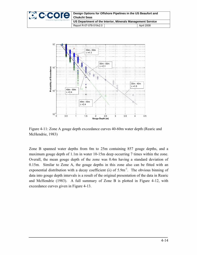
McHendrie, 1983) .................................................................................................. 4-13 Figure 4-11: Zone A gouge depth exceedance curves 40-60m water depth (Rearic and
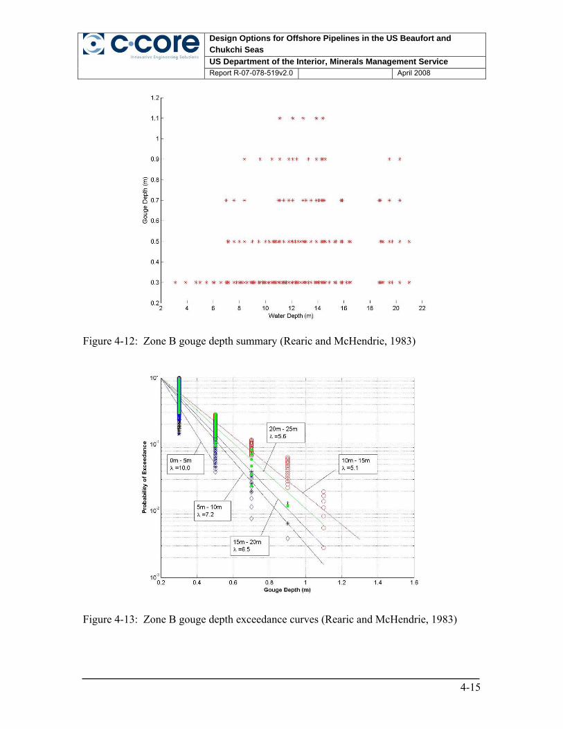
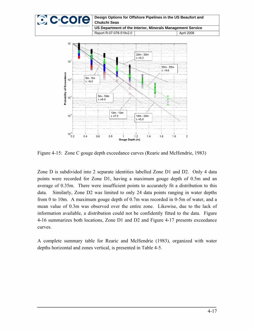
McHendrie, 1983) .................................................................................................. 4-14 Figure 4-12: Zone B gouge depth summary (Rearic and McHendrie, 1983) ............... 4-15 Figure 4-13: Zone B gouge depth exceedance curves (Rearic and McHendrie, 1983) 4-15 Figure 4-14: Zone C gouge depth summary (Rearic and McHendrie, 1983) ............... 4-16 Figure 4-15: Zone C gouge depth exceedance curves (Rearic and McHendrie, 1983) 4-17 Figure 4-16: Zone D gouge depth summary (Rearic and McHendrie, 1983)............... 4-18 Figure 4-17: Zone D gouge depth exceedance curves (Rearic and McHendrie, 1983) 4-18 Figure 4-18: Zone A gouge depth summary - known age (Weber et al., 1989) ........... 4-20 Figure 4-19: Zone B gouge depth summary – known age (Weber et al., 1989)........... 4-21 Figure 4-20: Zone C gouge depth summary – known age (Weber et al., 1989)........... 4-22 Figure 4-21: Gouge depth exceedance curves for single keel events (Weber et al., 1989)
................................................................................................................................ 4-24 Figure 4-22: Gouge depth exceedance curves for multiple keel events (Weber et al.,
1989) ...................................................................................................................... 4-24 Figure 4-23: Northstar gouge depth exceedance plot ................................................... 4-25 Figure 4-24: Mean gouge depth comparison of zoned datasets.................................... 4-26 Figure 4-25: Ratio between means of new and existing gouge depths as a function of
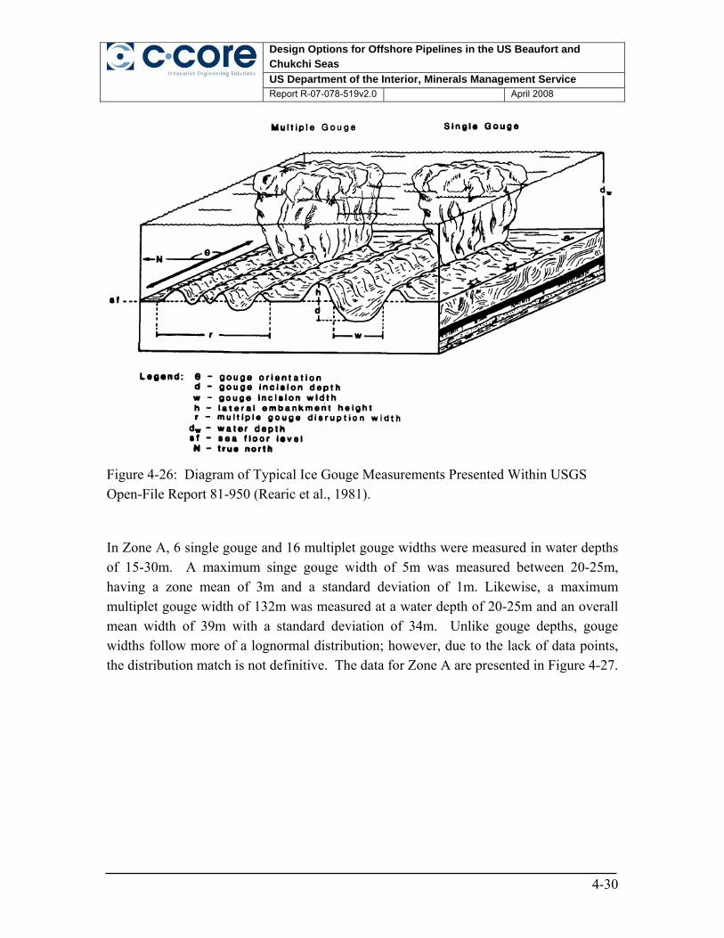
water depth in Canadian Beaufort Sea (Nessim and Hong, 1992) ........................ 4-27 Figure 4-26: Diagram of Typical Ice Gouge Measurements Presented Within USGS
Open-File Report 81-950 (Rearic et al., 1981). ..................................................... 4-30 Figure 4-27: Zone A gouge width summary for single and multiplet gouges (Weber et
al., 1989) ................................................................................................................ 4-31 Figure 4-28: Zone B gouge width summary for single and multiplet gouges (Weber et
al., 1989) ................................................................................................................ 4-32 Figure 4-29: Zone C gouge width summary for single and multiplet gouges (Weber et
Design Options for Offshore Pipelines in the US Beaufort and Chukchi Seas US Department of the Interior, Minerals Management Service
Report R-07-078-519v2.0 April 2008
x
Figure 4-32: Northstar gouge width exceedance plot ................................................... 4-36 Figure 4-33: Mean gouge width comparison of zoned datasets ................................... 4-37 Figure 4-34: Zone A crossing density (Rearic and McHendrie 1983).......................... 4-39 Figure 4-35: Zone B crossing density (Rearic and McHendrie 1983).......................... 4-40 Figure 4-36: Zone C crossing density (Rearic and McHendrie 1983).......................... 4-41 Figure 4-37: Zone D crossing density (Rearic and McHendrie 1983).......................... 4-42 Figure 4-38: Zone A crossing density (Weber et al., 1989).......................................... 4-44 Figure 4-39: Zone B crossing density (Weber et al., 1989).......................................... 4-45 Figure 4-40: Zone C crossing density (Weber et al., 1989).......................................... 4-46 Figure 4-41: Zone B crossing frequency (Weber et al., 1989) ..................................... 4-50 Figure 4-42: Zone C crossing frequency (Weber et al., 1989) ..................................... 4-51 Figure 5-1: Chukchi Sea case study zones...................................................................... 5-2 Figure 5-2: Toimil (1978) track lines.............................................................................. 5-4 Figure 5-3: Completed geo-hazard site specific surveys for the Chukchi Sea OCS waters
.................................................................................................................................. 5-7 Figure 5-4: Example of bathymetry and seafloor features map for plate 3 of the Popcorn
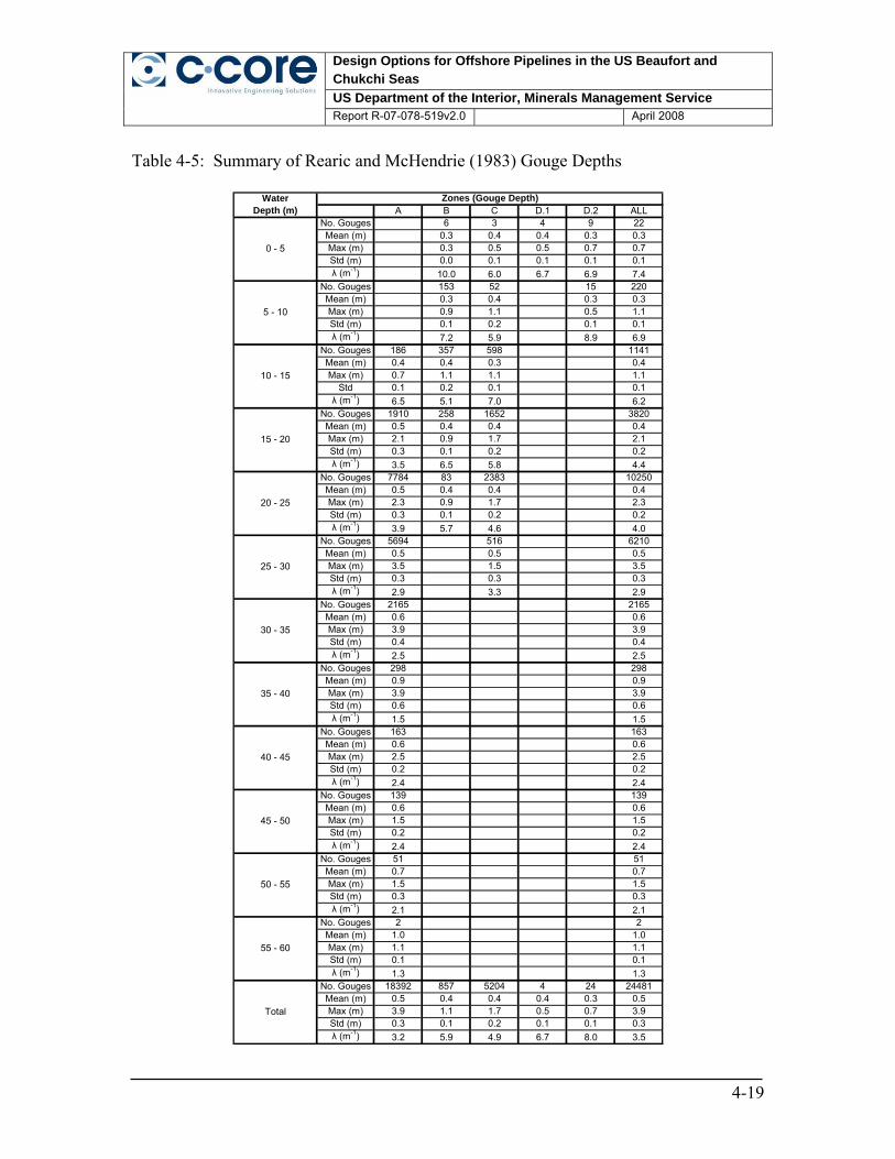
Prospect (Campbell and Rosendahl, 1990).............................................................. 5-9 Figure 5-5: Zone A maximum gouge depth summary (Toimil 1978) .......................... 5-10 Figure 5-6: Zone A gouge depth exceedance curve (Toimil 1978) .............................. 5-11 Figure 5-7: Zone C max gouge depth summary (Toimil 1978).................................... 5-12 Figure 5-8: Zone C gouge depth exceedance curves (Toimil 1978)............................. 5-12 Figure 5-9: Zone A maximum gouge width summary (Toimil 1978) .......................... 5-14 Figure 5-10: Zone C maximum gouge width summary (Toimil 1978) ........................ 5-15 Figure 5-11: Zone A crossing rates (Toimil 1978) ....................................................... 5-17 Figure 5-12: Zone C Crossing Rates (Toimil 1978) ..................................................... 5-18 Figure 6-1: Strudel scours in Beaufort Sea ..................................................................... 6-1 Figure 6-2: Zoned strudel scours in Beaufort Sea .......................................................... 6-4 Figure 6-3: Beaufort Sea strudel scour depth summary.................................................. 6-5 Figure 6-4: Mean strudel scour depths............................................................................ 6-6 Figure 6-5: Strudel scour depth exceedance distribution................................................ 6-6 Figure 6-6: Beaufort Sea strudel scour width summary ................................................. 6-7 Figure 6-7: Mean strudel scour widths ........................................................................... 6-8 Figure 6-8: Strudel scour width exceedance distribution ............................................... 6-8 Figure 7-1: Assumed failure mechanism during an ice gouge event in sand (Phillips et
al., 2005) .................................................................................................................. 7-5 Figure 7-2: Comparison of measured and calculated gouge forces in sand (Phillips et al.,
Design Options for Offshore Pipelines in the US Beaufort and Chukchi Seas US Department of the Interior, Minerals Management Service
Report R-07-078-519v2.0 April 2008
xi
Figure 7-3: Observed subgouge deformations in sand over clay (Phillips et al., 2005) . 7-6 Figure 7-4: Soil particle trajectories during ice gouge events (Kenny et al., 2007a) ... 7-10 Figure 7-5: Series of tracer particles mapping the three dimensional subgouge
deformation field. (Kenny et al., 2007b)................................................................ 7-11 Figure 7-6: Vertical profile of sub-gouge deformations from numerical and centrifuge
studies (Kenny et al., 2007b) ................................................................................. 7-12 Figure 7-7: Soil failure mechanism and distribution of equivalent plastic strain (Kenny et
al., 2007b) .............................................................................................................. 7-12 Figure 7-8: Soil spring representation (ASCE 1984).................................................... 7-14 Figure 7-9: Coupled ice keel/seabed/pipeline interaction model using continuum and
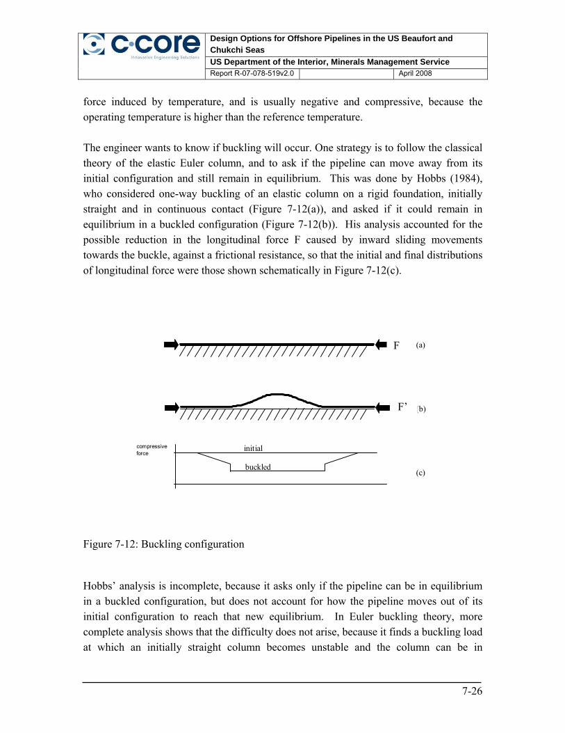
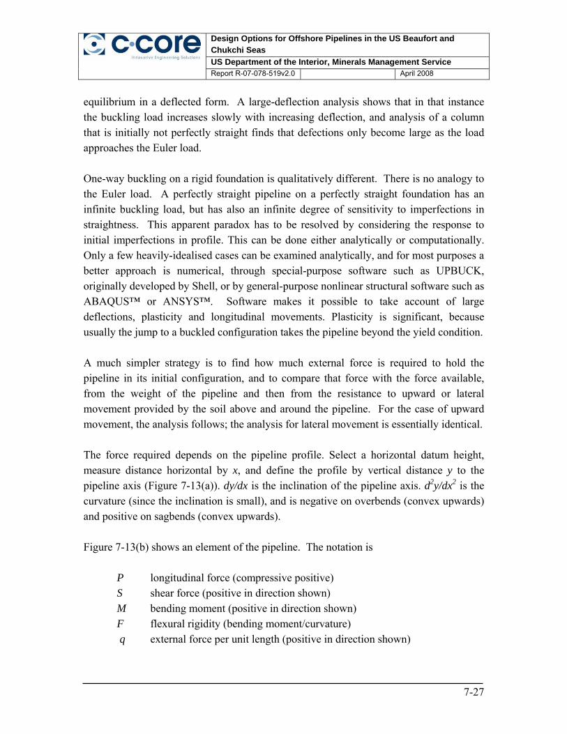
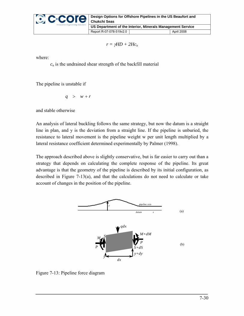
structural elements ................................................................................................. 7-16 Figure 7-10: Hjulstrom chart for predicting erosion susceptibility of seabed soils ...... 7-20 Figure 7-11: Interpreted strudel scour slope angles from MMS (2002) ....................... 7-21 Figure 7-12: Buckling configuration ............................................................................. 7-26 Figure 7-13: Pipeline force diagram .............................................................................. 7-30 Figure 7-14: Driving force diagrams (a) under normal operating conditions and (b) under
the effect of ice gouging ........................................................................................ 7-34 Figure 8-1: Buckled mode for (a) no internal pressure and (b) internal pressure of a spiral
linepipe subjected to moment loading (Zimmerman et al., 2004) ........................... 8-4 Figure 8-2: Generalized moment curvature relationship for pipeline subject to combined
state of loading......................................................................................................... 8-5 Figure 8-3: Numerical prediction of pipeline moment-curvature response as a function of
D/t ratio for a constant pressure stress ratio and end moment loading (Fatemi et al., 2006) ........................................................................................................................ 8-6
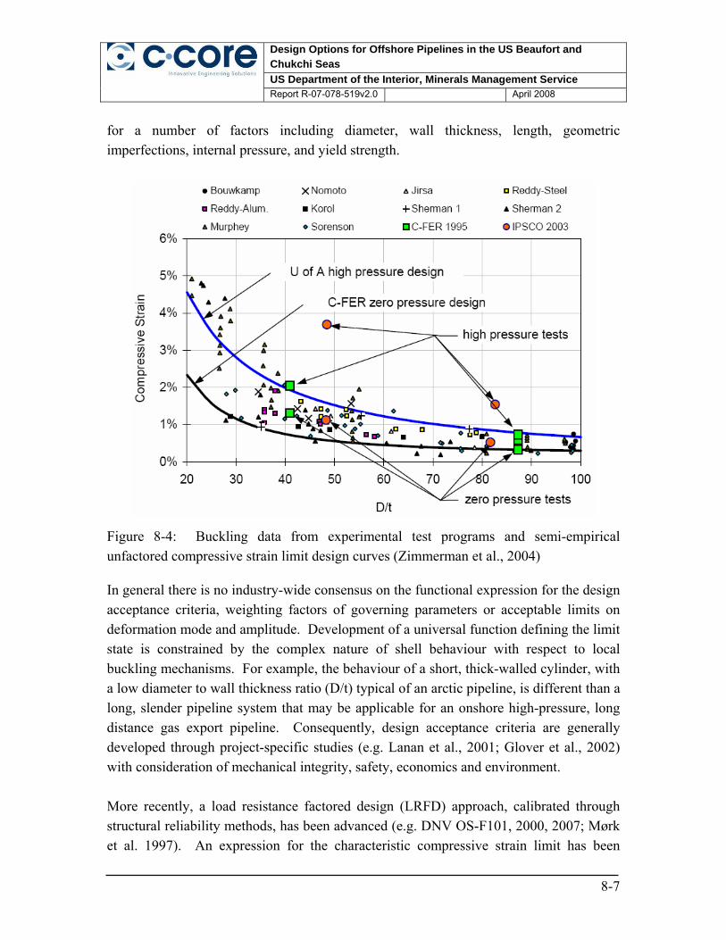
Figure 8-4: Buckling data from experimental test programs and semi-empirical unfactored compressive strain limit design curves (Zimmerman et al., 2004)........ 8-7
Figure 8-5: Moment-curvature response for a pipeline with different D/t ratios subject to a constant compressive axial force (750kN) and end moment loading ................... 8-9
Figure 9-1: Procedure used in pipeline burial analysis................................................... 9-2 Figure 9-2: Illustration of gouge geometry and pipeline clearance ................................. 9-4 Figure 9-3: Pipeline cover depth example ...................................................................... 9-8 Figure 9-4: Sensitivity of mean gouge depth to pipeline cover depth requirement......... 9-9 Figure 9-5: Sensitivity of mean gouge width to pipeline cover depth requirement........ 9-9 Figure 9-6: Sample pipeline route................................................................................. 9-10 Figure 9-7: Pipeline water depth distribution ............................................................... 9-11 Figure 9-8: Mean gouge depth versus water depth....................................................... 9-12 Figure 9-9: US & Canadian Crossing Rate Comparison .............................................. 9-13
Design Options for Offshore Pipelines in the US Beaufort and Chukchi Seas US Department of the Interior, Minerals Management Service
Report R-07-078-519v2.0 April 2008
xii
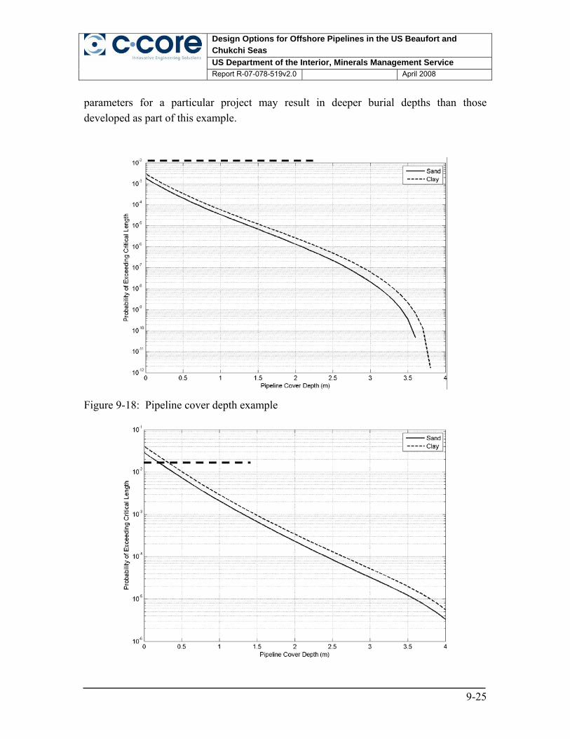
Figure 9-10: Pipeline crossing rate and mean gouge depth distribution....................... 9-14 Figure 9-11: Burial depth analysis for 15 to 25km pipeline interval ............................ 9-15 Figure 9-12: Cover depth requirements along pipeline route ....................................... 9-16 Figure 9-13: Procedure used in pipeline burial analysis............................................... 9-18 Figure 9-14: Strudel scour alignment – centred (offset = 0) and edge (offset = 1) ...... 9-20 Figure 9-15: Illustration of strudel scour geometry ...................................................... 9-21 Figure 9-16: Allowable pipeline unsupported span ...................................................... 9-23 Figure 9-17: Pipeline stability plot ............................................................................... 9-23 Figure 9-18: Pipeline cover depth example .................................................................. 9-25 Figure 9-19: Sensitivity of pipeline cover depth to scour geometry – cylindrical shape .9-
26 Figure 9-20: Sensitivity of pipeline cover depth to mean scour diameter of 18m........ 9-26 Figure 10-1: Northstar on-ice trench excavation trials (INTEC, 2006)......................... 10-3 Figure 10-2: Gravel island approach excavation as sidebooms lower the Northstar
pipeline bundle 50 ft to the seafloor (INTEC, 2000) ............................................. 10-5 Figure 10-3: Through-ice installation of the Oooguruk pipeline bundle (H.C. Price Co.,
2008) ...................................................................................................................... 10-5 Figure 10-4: Through-ice installation of the Oooguruk pipeline bundle (H.C. Price Co.,
Design Options for Offshore Pipelines in the US Beaufort and Chukchi Seas US Department of the Interior, Minerals Management Service
Report R-07-078-519v2.0 April 2008
1-1
1 INTRODUCTION
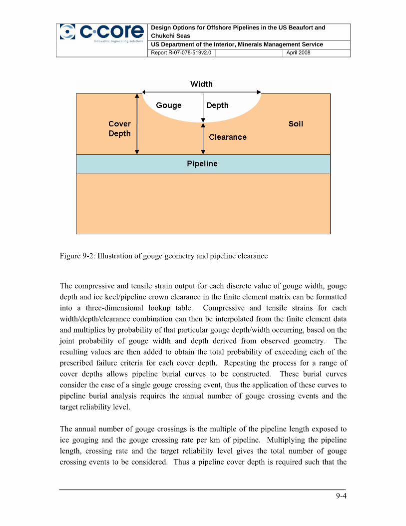
The design of arctic pipelines and protection requirements for mechanical integrity are driven by hazards such as ice gouging, strudel scour and upheaval buckling. The pipeline wall thickness, line-pipe grade and ductility, trench depth and backfill requirements are some of the key factors for consideration in pipeline engineering design. This study addresses the requirements of the Minerals Management Service (MMS) Contract M-07-PC-13015 as part of Technology Assessment and Research (TAR) Project 577. The objective of the study, based on the request for proposals from MMS is to “assess the design options for pipelines and provide a risk analysis for strudel scour, upheaval buckling and ice gouging in the Beaufort and Chukchi Seas”. The project team comprised of specialists with considerable experience in the research, design and operations of offshore pipelines in the Arctic. The team was made up of:
• C-CORE was Project Manager for this study and led the interpretation of ice gouge and strudel scour survey data, implementation of design models and burial depth analyses.
• Andrew Palmer of Bold Island Engineering provided an overview of pipeline buckling and its consideration in Arctic conditions based on his extensive experience of pipeline design and construction. He also provided valuable input throughout the study.
• Mike Paulin of IMVPA provided a review of existing ice gouge survey data and Arctic pipeline construction, inspection and repair methodologies for Arctic pipelines based on experience gained from several pipeline projects in this region.
• Shawn Kenny of Memorial University of Newfoundland provided specialist input into the discussion of numerical modeling and strain demand of pipelines under ice gouge loading based on current research activities.
1.1 Ice Gouging
Ice ridging occurs in arctic regions such as the Beaufort and Chukchi Seas as a result of the formation of pressure ridges as ice sheets collide and deform under the influence of winds and other environmental effects. Pressure ridges may be composed of either first-year or multi-year ice, and comprise a sail as ice is deformed upward above the waterline,
Design Options for Offshore Pipelines in the US Beaufort and Chukchi Seas US Department of the Interior, Minerals Management Service
Report R-07-078-519v2.0 April 2008
1-2
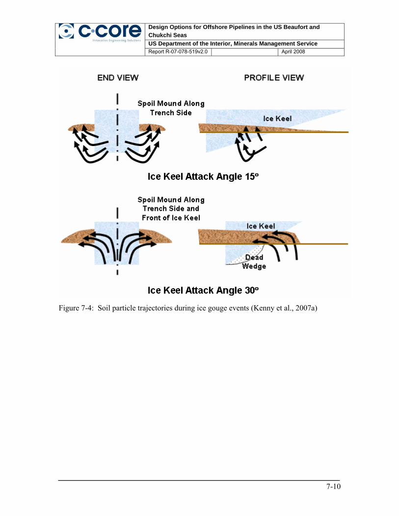
and a keel extending below water. The keel then poses a risk of grounding and penetrating the seabed as the ice continues to move under the influence of the environmental driving forces, resulting in furrows, or gouges in the seabed. The ice gouging process is illustrated in Figure 1-1.
Figure 1-1: Schematic of gouging ice ridge keel
The most important parameters in assessing ice gouge risk to pipelines are the gouge rate, gouge depth and gouge width. Data that can be used for ice keel gouge assessment is usually sparse, but this section reviews the available information from the Beaufort and Chukchi Seas. The formation rate of ice gouges is typically inferred from repetitive mapping of the seabed. Repetitive mapping consists of comparing surveys of the same portion of the seabed conducted at least one year apart so that new gouges can be identified. In the Beaufort Sea these surveys usually consist of long lines of limited lateral extent, thus the formation rate of gouges is expressed in terms of the number of gouge crossings per unit distance of survey line per unit time (i.e. km-1yr-1). When interpreting gouge rates or comparing gouge rates from different sources, care must be exercised that the gouge rate and gouge geometry are consistent. Gouge crossing rates may exclude gouges below a certain threshold (i.e. typically 0.1 to 0.2 m), or may in some cases include gouge events with depths less than the resolution of the depth profiler. While these sub-resolution gouges may be left out of the gouge depth distribution (resulting in higher mean gouge
Design Options for Offshore Pipelines in the US Beaufort and Chukchi Seas US Department of the Interior, Minerals Management Service
Report R-07-078-519v2.0 April 2008
1-3
depths), they may have been included in the gouge rate (Nessim and Hong, 1992), which would lead to a level of conservatism in the resulting analyses. The treatment of single keel and multi-keel gouges (a group of ice gouges considered to be part of the same event based on temporal and spatial proximity) must also be considered. In most analyses, multi-keel gouges were counted as single events, rather than considering each gouge comprising the multi-keel gouge as a separate entity. In order to maintain consistency, the gouge geometry (in particular the gouge depth distribution) should reflect this grouping of gouges into a single event. Thus the maximum gouge depth would be the deepest of all the gouges in the multi-keel event. Assigning the appropriate gouge width can present a challenge since gouges comprising multi-keel events can be separated by appreciable distances – in excess of 100 meters (Campbell, 2006). Judgement is thus needed to assign an appropriate and consistent width to the gouge data in question. Available data from USGS sources have been reviewed and processed to provide a basis for estimating geometric characteristics and event density or frequency of occurrence for ice gouging and strudel scour in the US Beaufort and Chukchi Seas. A limited dataset was available for use, and the data were primarily collected in the late 1970s and 1980s. More up-to-date data are largely proprietary and not available for this study. The data have been processed to derive distributions of gouge depth and width as a function of location (zones) and water depth in the most appropriate way for the data available. Although values have been derived and presented for all zones where data exist, the level of confidence attributed to the data is limited by the quality of the data for anything other than concept level and comparative studies. Significant additional survey work would be required to provide the increased confidence required for detailed pipeline routing and design. Specific limitations to be considered with respect to interpreting ice gouge surveys include the following:
• Side scan survey techniques used for data collection undergo subjective interpretation of paper records for geometry and frequency of seabed features by USGS personnel, and the original records are not easily available for reanalysis.
Design Options for Offshore Pipelines in the US Beaufort and Chukchi Seas US Department of the Interior, Minerals Management Service
Report R-07-078-519v2.0 April 2008
1-4
• Data summaries do not always provide all the required data e.g. only maximum gouge depths and widths within a given survey segment are given rather than data for all gouge events.
• Non-repetitive surveys record ice gouge or strudel scour events of unknown ages, which make it difficult to interpret return frequencies. Further, seabed features may have been present for months or years prior to surveying, and may have been subjected to infilling or other processes that altered their geometry over time. Geometric distributions may therefore be inaccurate.
• Repetitive mapping on an annual basis is limited to a small number of survey lines, which provides a limited means for direct comparison of statistics for gouges of unknown ages. The opposing effect of sediment infilling and the likelihood of recording more extreme events in non-repetitive surveys provide difficulty in properly assessing accurate geometric parameters.
• Gouge depth resolutions are not always consistent between different surveys, which can lead to difficulties in providing representative comparisons.
• Data for single and multiple keel events are not always presented consistently between surveys, which makes it difficult to provide direct comparisons.
• Extreme gouge depths and widths are presented in datasets, but often no explanation is provided on additional observations that may establish the validity of such measurements.
• Limited data in some zones and water depth increments may restrict the validity of curve fitting techniques, resulting in lower confidence levels for stated parameters.
In light of the above limitations, the statistical values developed from survey data as part of this report should be considered indicative only. Distributions can be applied to the data to develop geometrical fits, although in many cases, the lack of data points limit the accuracy of these curves. Some cases suggest that the curves under-predict the measured probability of exceedance and could be under-conservative. Extrapolation of curves beyond the available data should be used with caution, as a maximum practical depth or width, based on the physical ice gouging process would be expected to occur as a function of ice driving forces, ice keel strength and soil type and strength. Judgement must be exercised in developing such design parameters.
Design Options for Offshore Pipelines in the US Beaufort and Chukchi Seas US Department of the Interior, Minerals Management Service
Report R-07-078-519v2.0 April 2008
1-5
1.2 Strudel Scour
Nearshore Arctic zones typically develop a bottomfast ice sheet in shallow water during the winter. Craters in the seabed can be formed in the spring during river breakup when the river overfloods the nearshore landfast sea ice. This overflood water, typically 0.6 to 1.2 m deep, spreads offshore, up to 16 to 19 km seaward, and drains though holes in the ice sheet (e.g. tidal cracks, thermal cracks, and seal breathing holes). If the conditions are right, in that the water depth is relatively shallow and the drainage velocity through the holes in the ice sheet is high, seabed sediments can be eroded leaving a circular or linear scour in the seabed (Leidersdorf et al., 1996), which can potentially expose and impose high current loads on a pipeline as shown in Figure 1-2. This phenomenon is known as strudel scour. A number of environmental factors and processes may affect the magnitude and frequency of occurrence of strudel scour events, which include over-flooding (i.e. static head, spatial extent and temporal occurrence), river discharge (i.e. flow rates, effects of ice jams), and surface features (e.g. ice cover drainage cracks or fissures, snow cover, pressure ridges, frazil ice). There exist limited datasets to quantify and assess the importance of these parameters on strudel scour events and this impacts engineering uncertainty.
Figure 1-2: Strudel scour process
Design Options for Offshore Pipelines in the US Beaufort and Chukchi Seas US Department of the Interior, Minerals Management Service
Report R-07-078-519v2.0 April 2008
1-6
Some of the earliest studies included work by Reimnitz et al. (1974) who studied strudel scours in the US Beaufort using side-scan sonar, echosounder, high resolution seismic profiling, sediment sampling and direct observations from divers. Investigation of one strudel scour by divers is presented in Figure 1-3. Reimnitz and Kempema (1982a) observed and monitored the infilling of strudel scours in the US Beaufort Sea. The authors report generation rates of 2.5/km2/year and dimensions up to 25m wide and 6m deep. Scours which were monitored were in about 2.5m water depth and were originally 3 to 4m deep. Observations indicated that the strudel scours were infilled after 2 to 3 years. The authors conclude that, because of strudel scouring, the delta areas of arctic rivers should be totally reworked and consist of strudel scour deposits. It is also noted that the authors suggest the effects of most dredging and other construction activities might be insignificant in the strudel scour area as compared to natural sediment transport rates. Statistics of strudel scour events can be obtained by visual inspection of the seabed but are typically obtained through electronic seabed surveys (i.e. side-scan, multi-beam). For circular features, the radius and depth of the strudel scour is surveyed. For linear features, the depth, width, length and orientation characteristics are measured, where typical dimensions at the start of strudel scour are the largest magnitude. This later observation is important when examining statistics of the dataset. The geographical coordinates and water depth are also typically measured.
Figure 1-3: Strudel scour investigated by direct diving observations (Reimnitz et al., 1974)
Design Options for Offshore Pipelines in the US Beaufort and Chukchi Seas US Department of the Interior, Minerals Management Service
Report R-07-078-519v2.0 April 2008
1-7
Another important factor to address when examining strudel scour statistics is the effect of infilling that may occur immediately after the scour event. This would be due to settling of the seabed material held in transient suspension within the water column and through long-term sediment transport due to wave and current action. The rate of infilling for the US Beaufort Sea is location dependent and may range from 0.05m/year, in sheltered areas, to 2.5m/year at the head of river deltas or in exposed offshore locations. Infilling would tend to bias the statistical distribution of measured strudel scours to shallower depths. Limited sample size may affect confidence and data uncertainty. Due to cost and logistics, geotechnical parameters are generally not obtained. This limits the potential development of engineering relationships to correlate geotechnical data, such as soil type, grain size, submerged unit weight, relative density, and soil strength, with infilling and strudel scour resistance mechanisms. It is unlikely that every drain hole in the sheet ice produces a scour in the seafloor. The deepest scour depressions are found in shallow water (e.g., 2 to 3m deep) where the strudel flow is sufficiently powerful to excavate the seafloor sediments immediately below the ice. If a strudel scour happens on top of a pipeline alignment, there is the possibility that the scour could result in an unacceptable pipeline span. In extreme conditions, the pipeline span could possibly experience vortex-induced vibration (VIV) due to the water velocity of the strudel flow. An analysis to assess the pipeline span can be carried out using analytical or finite element methods. The analyses can be carried out to account for gravity, thermal, pressure and hydrodynamic loads. The potential for Vortex-Induced Vibrations (VIV) of the pipeline from the strudel flow can also be evaluated. Strudel scour and the resulting unsupported pipeline spans which they potentially may produce are possibly important issues for the design of offshore arctic pipelines. However, the problem must be considered in light of current industry design/operation capabilities. The importance placed on potential strudel scour issues is possibly the result of the use of conservatisms to compensate for lack of knowledge of the physical processes involved. This suggests that there is design optimization work that needs to be carried out to remove conservatism including: investigation into the strudel scour formation process
Design Options for Offshore Pipelines in the US Beaufort and Chukchi Seas US Department of the Interior, Minerals Management Service
Report R-07-078-519v2.0 April 2008
1-8
and the associated water flow velocities which may apply loads to a pipeline; better definition of VIV of a pipeline exposed to a water jet vortex beneath a strudel scour during creation; the mechanical response of a pipeline exposed and suspended across a strudel scour hole; and any preferential creation of strudel scours in the warmer region around a pipeline operated at a temperature greater than ambient (such as that possibly observed by Leidersdorf et al., 2006). Not all pit like depressions seen in the Beaufort are caused by strudel flow. Some of these depressions may have been caused by ice wallowing, which is described as local seabed erosion around grounded ice features due to local ocean current flow disturbances and wave-induced motion of the ice feature displacing water and sediment. Numerous irregular seabed depressions and mounds, with up to 3m vertical relief and 100m in diameter, have been observed offshore Reindeer Island (15 km east of Seal Island) in 3 to 6m water depths in the Alaskan Beaufort Sea (Reimnitz and Kempema, 1982b). 1.3 Upheaval Buckling
A pipeline can buckle either upwards (‘upheaval buckling’) or sideways (‘lateral buckling’); occasionally the two occur together. Upheaval buckling generally occurs in trenched and buried pipelines, because it is easier for the pipeline to move upwards, against the weight and resistance of the overlying backfill material, than it is for the line to move sideways, against the comparatively high passive resistance of the undisturbed soil on either side of the trench. Buckles almost invariably occur at overbends, where the pipe profile is convex upwards, and the pipeline moves from an unbuckled configuration (Figure 1-4(a)) to a buckled one (Figure 1-4(b)), often by a sudden ‘jump’. Figure 1-5 is a photograph of upheaval buckling in a 1020 mm (40 inch) land pipeline in Uzbekistan. Upheaval is well known in land pipelines, and there are many examples, from Iran, Russia, the United Arab Emirates and elsewhere. Lateral buckling generally occurs in unburied pipelines, because they often have less resistance to sideways movement than to upward movement. A pipeline moves sideways against the friction of whatever it is lying on, whereas if it lifts upwards its own weight resists the movement. Many marine pipelines are not trenched or buried, and so lateral buckling mostly occurs in marine pipelines, but it does sometimes occur in land pipelines trenched in very soft soils. Marine Arctic pipelines are, however, usually trenched and buried. Figure 1-6 shows a laterally buckled pipeline in Siberia, and Figure 1-7 is a
Design Options for Offshore Pipelines in the US Beaufort and Chukchi Seas US Department of the Interior, Minerals Management Service
Report R-07-078-519v2.0 April 2008
1-9
photograph looking downwards on a pipeline in Brazil that has buckled laterally in soft mud; the caption points to soil that has been pushed sideways by the moving pipeline. Lateral buckles are initiated by horizontal out-of-straightness.
initial
buckled
(a)
(b)
Figure 1-4: Upheaval buckling of pipeline at overbend
Design Options for Offshore Pipelines in the US Beaufort and Chukchi Seas US Department of the Interior, Minerals Management Service
Report R-07-078-519v2.0 April 2008
1-10
Figure 1-5: Example of upheaval buckling
Figure 1-6: Example of onshore lateral buckling
Design Options for Offshore Pipelines in the US Beaufort and Chukchi Seas US Department of the Interior, Minerals Management Service
Report R-07-078-519v2.0 April 2008
1-11
SOLO DESLOCADO PELA DEFORMAÇÃO DO DUTO
Figure 1-7: Example of offshore lateral buckling
Design Options for Offshore Pipelines in the US Beaufort and Chukchi Seas US Department of the Interior, Minerals Management Service
Report R-07-078-519v2.0 April 2008
2-1
2 BEAUFORT SEA – ENVIRONMENTAL CONDITIONS
2.1 General
The US Beaufort Sea extends from the Alaska-Yukon border in the east to Point Barrow in the west, and the continental shelf extends to a shelf break at between 60 and 120km from shore at water depths of 60 to 70m. The major bathymetric features in the shelf are the barrier islands (that extend to several metres above sea level) and shoals (rising 5 to 10m above the surrounding seabed) that lie in a chain parallel to the shoreline in water depths of 10 to 20m. Ongoing erosion and deposition leads to migration of the islands at rates of approximately 20 to 30m/year to the west. Significant micro-relief is also present as a result of interaction between drift ice ridge keels and the seabed. The western edge of the Beaufort Sea shelf terminates at the Barrow Sea Valley, which extends to depths greater than 100m north of Point Barrow. Figure 2-1 presents a location plan and bathymetry of the Alaskan Beaufort Sea (MMS, 2002). 2.2 Geotechnical Profile
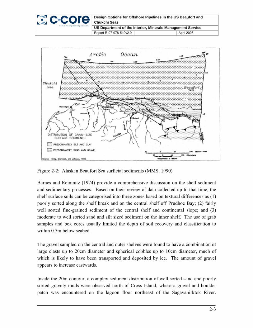
The surficial sediments of the Alaskan Beaufort Sea continental shelf consist predominantly of clay to silt sized soil particles, although course grained sediments are found in the near-shore areas, in the vicinity of offshore barrier islands, on shoals and along the shelf break as shown in Figure 2-2 (MMS, 1990). The seabed sediments are generally over-consolidated as a function of historical glaciation and current erosional regime.
Design Options for Offshore Pipelines in the US Beaufort and Chukchi Seas US Department of the Interior, Minerals Management Service
Report R-07-078-519v2.0 April 2008
2-2
Figure 2-1: Alaskan Beaufort Sea plan and bathymetry (MMS, 2002)
Design Options for Offshore Pipelines in the US Beaufort and Chukchi Seas US Department of the Interior, Minerals Management Service
Barnes and Reimnitz (1974) provide a comprehensive discussion on the shelf sediment and sedimentary processes. Based on their review of data collected up to that time, the shelf surface soils can be categorised into three zones based on textural differences as (1) poorly sorted along the shelf break and on the central shelf off Prudhoe Bay; (2) fairly well sorted fine-grained sediment of the central shelf and continental slope; and (3) moderate to well sorted sand and silt sized sediment on the inner shelf. The use of grab samples and box cores usually limited the depth of soil recovery and classification to within 0.5m below seabed. The gravel sampled on the central and outer shelves were found to have a combination of large clasts up to 20cm diameter and spherical cobbles up to 10cm diameter, much of which is likely to have been transported and deposited by ice. The amount of gravel appears to increase eastwards. Inside the 20m contour, a complex sediment distribution of well sorted sand and poorly sorted gravely muds were observed north of Cross Island, where a gravel and boulder patch was encountered on the lagoon floor northeast of the Sagavanirktok River.
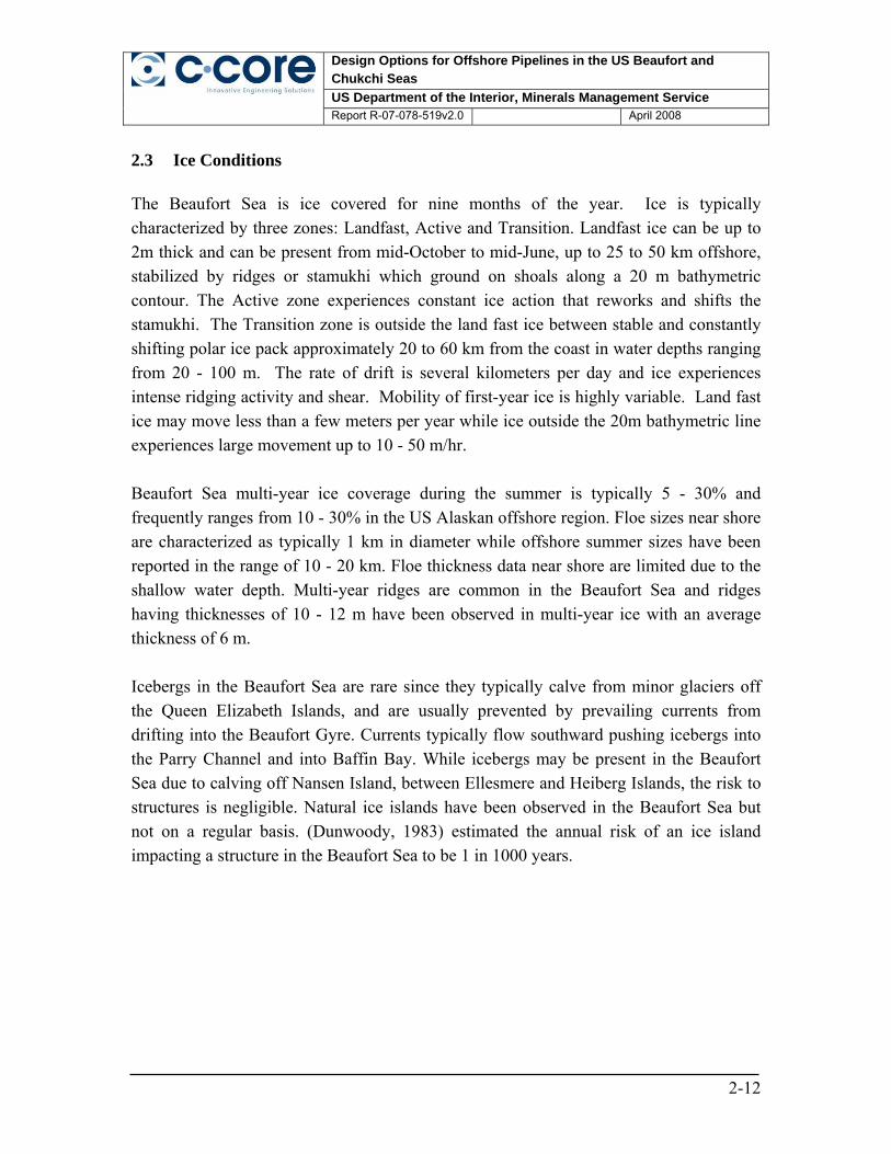
Design Options for Offshore Pipelines in the US Beaufort and Chukchi Seas US Department of the Interior, Minerals Management Service
Report R-07-078-519v2.0 April 2008
2-4
Outcrops of stiff silty clay were also observed in this area. Figure 2-3 to Figure 2-5 present distributions of surface soils in terms of grain size, sorting and gravel content reported by Barnes & Reimnitz (1974). Reimnitz et al. (1977) provide some soil description and shear strength data from vibrocore samples and in-situ testing in the Alaskan Beaufort Shelf, as well as pore fluid salinity and temperature profiles. Figure 2-6 presents the sample and test locations. Soil type and strength data are limited to the top 10cm or so below the seabed and is generally described as soft sandy or gravely mud, although stiffer clays are noted at some locations. Recorded shear strength is mainly very soft, and is indicative of the shallow sediments. The effect of sample disturbance and reworking due to intense ice gouging is also likely to have affected the samples. Four general categories were identified in the top 50m of seabed soils, as described below:
• Soft to medium stiff fine grained Holocene deltaic, marine and lagoon deposits. These low to medium plasticity silts and clays have properties that vary with depth. Strength values vary inversely with moisture content and are typically around 35kPa in the upper portion, decreasing to 25kPa in the lower portion. Organic, high plastic lagoon and marine clays were found to have strengths on the order of 5 to 40kPa, with an average of 20kPa. The thickness of this deposit varied from 3 to 12m below seabed where it was encountered, mainly shoreward of the barrier islands in Prudhoe Bay and Mikkelsen Bay.
• Medium dense to very dense, uniform fine sand found in Holocene shoal deposits.
The sand particles are described as very angular having a mean grain size of 0.11 and 0.19mm. Standard penetration values measured during boring were generally between 10 and 75 per 300mm, and a measured internal angle of friction was 41° to 47°. This material, between 1 and 4m thick, was found adjacent to and just offshore the barrier islands and are linked with underwater shoals.
• Stiff to hard, Pleistocene silt and clay deposits with undrained shear strengths
measured in the range 50 to 300kPa, with an average value of 130kPa. Soft zones were also noted during drilling, but not sampled. These stiff clays generally underlie the Holocene deposits, although were not encountered in all locations. This soil was also encountered at the seabed, having a thickness of between 11
Design Options for Offshore Pipelines in the US Beaufort and Chukchi Seas US Department of the Interior, Minerals Management Service
Report R-07-078-519v2.0 April 2008
2-5
and 35m in a zone between Cross Island and Stefansson Sound, and also to the east of the Maguire Islands.
• Dense, well graded Pleistocene sand and gravel generally underlies the
Pleistocene clays, although it was occasionally sampled directly below the Holocene deposits. The material is reasonably well graded and varies in particle size up to a maximum of 50mm diameter. The depth to the surface of this sand and gravel layer increases with distance from shore, and also from west to east, from about 3m to in excess of 100m.
Temperature profiling and sample observation also allowed the presence of ice-bonded permafrost to be determined. The top of the permafrost was limited to the Pleistocene deposits between 15 and 60m below seabed, but was encountered as shallow as 7m in one borehole. Figure 2-8 presents typical borehole logs from this survey, and Figure 2-9 provides stratigraphic cross-sections of selected lines across the survey area, as defined in Figure 2-7. Miller & Bruggers (1980) describe a geotechnical field program that drilled 20 boreholes in the Alaskan Beaufort Sea between the Kuparuk River and Canning River deltas, with the aim of determining geotechnical and permafrost properties of the near seabed soils in this region. Figure 2-7 shows a location map of the boreholes and Table 2-1 presents a summary of soil conditions.
Design Options for Offshore Pipelines in the US Beaufort and Chukchi Seas US Department of the Interior, Minerals Management Service
Report R-07-078-519v2.0 April 2008
2-6
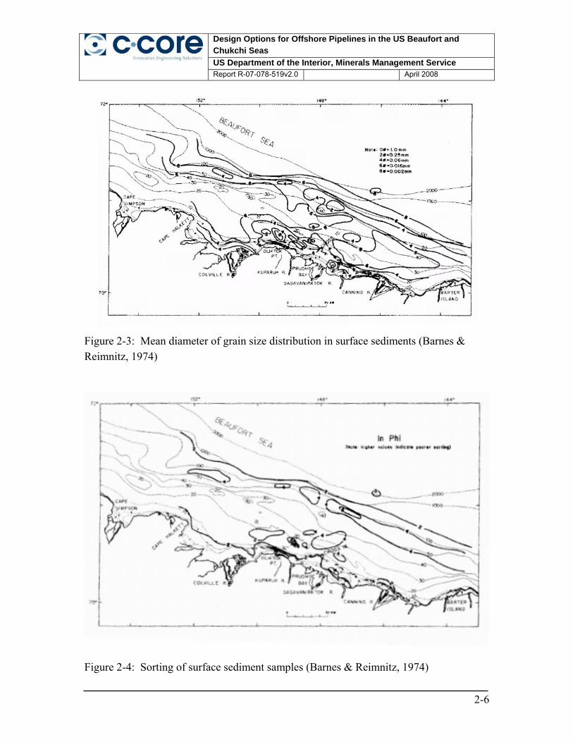
Figure 2-3: Mean diameter of grain size distribution in surface sediments (Barnes & Reimnitz, 1974)
Design Options for Offshore Pipelines in the US Beaufort and Chukchi Seas US Department of the Interior, Minerals Management Service
Report R-07-078-519v2.0 April 2008
2-10
(a) (b)
(c) (d)
(a) (b)
(c) (d)
Figure 2-8: Borehole logs typical of (a) borings 1, 2, 3, 5 and 15, (b) 4, 10, 11 and 16, (c) 6, 7, 14 and 19, (d) 8, 9, 12, 13, 17, 18 and 20 (Miller & Bruggers, 1980)
Design Options for Offshore Pipelines in the US Beaufort and Chukchi Seas US Department of the Interior, Minerals Management Service
Report R-07-078-519v2.0 April 2008
2-11
Figure 2-9: Stratigraphic sections AA, BB and CC (Miller & Bruggers, 1980)
Design Options for Offshore Pipelines in the US Beaufort and Chukchi Seas US Department of the Interior, Minerals Management Service
Report R-07-078-519v2.0 April 2008
2-12
2.3 Ice Conditions
The Beaufort Sea is ice covered for nine months of the year. Ice is typically characterized by three zones: Landfast, Active and Transition. Landfast ice can be up to 2m thick and can be present from mid-October to mid-June, up to 25 to 50 km offshore, stabilized by ridges or stamukhi which ground on shoals along a 20 m bathymetric contour. The Active zone experiences constant ice action that reworks and shifts the stamukhi. The Transition zone is outside the land fast ice between stable and constantly shifting polar ice pack approximately 20 to 60 km from the coast in water depths ranging from 20 - 100 m. The rate of drift is several kilometers per day and ice experiences intense ridging activity and shear. Mobility of first-year ice is highly variable. Land fast ice may move less than a few meters per year while ice outside the 20m bathymetric line experiences large movement up to 10 - 50 m/hr. Beaufort Sea multi-year ice coverage during the summer is typically 5 - 30% and frequently ranges from 10 - 30% in the US Alaskan offshore region. Floe sizes near shore are characterized as typically 1 km in diameter while offshore summer sizes have been reported in the range of 10 - 20 km. Floe thickness data near shore are limited due to the shallow water depth. Multi-year ridges are common in the Beaufort Sea and ridges having thicknesses of 10 - 12 m have been observed in multi-year ice with an average thickness of 6 m. Icebergs in the Beaufort Sea are rare since they typically calve from minor glaciers off the Queen Elizabeth Islands, and are usually prevented by prevailing currents from drifting into the Beaufort Gyre. Currents typically flow southward pushing icebergs into the Parry Channel and into Baffin Bay. While icebergs may be present in the Beaufort Sea due to calving off Nansen Island, between Ellesmere and Heiberg Islands, the risk to structures is negligible. Natural ice islands have been observed in the Beaufort Sea but not on a regular basis. (Dunwoody, 1983) estimated the annual risk of an ice island impacting a structure in the Beaufort Sea to be 1 in 1000 years.
Design Options for Offshore Pipelines in the US Beaufort and Chukchi Seas US Department of the Interior, Minerals Management Service
Report R-07-078-519v2.0 April 2008
3-1
3 CHUKCHI SEA – ENVIRONMENTAL CONDITIONS
3.1 General
The US Chukchi Sea is located in the Arctic Ocean northwest of the Alaskan coast, generally between Point Barrow to the east and Cape Prince of Wales to the west. The offshore area is characterized by a broad shelf with subtle relief, sloping gently to the north. Water depths are generally in the range of 30 to 60m on the shelf, dropping sharply to greater than 3000m to the north and east into the Arctic Basin, as presented in Figure 3-1. The Barrow Valley forms a deep channel to the north west of Point Barrow, with a depth of up 100m. The broader, shallow Hope Valley is present to the south west of Point Hope, having a depth of the order of 50m. A number of shoals are also present within the shelf area, including Herald Shoal to the west and Hanna Shoal to the east, each with local high points extending to within 20m of the surface, and a broad area in between with 35m to 40m depth. A number of isolated shoals are also present in the nearshore region along the north and west coast in 20 to 30m water depth. These shoals serve to capture deep draft ice features as they drift into the Chukchi Sea, thereby limiting potential ice gouging of the seabed. 3.2 Geotechnical Profile
Seabed sediments can be classified as thin surficial sediments, overlying bedrock, which frequently outcrops at the seabed in water depths greater than 30m. Most of the shelf area was sub-aerially exposed during Pleistocene low sea levels, inducing permafrost, which could still be present in a relict form (Toimil, 1978). Quaternary sediment cover is generally thin over the central shelf area, between 2 and 10m thick in water depths greater than 30m, although local infilling of troughs in the bedrock allows thicknesses to exceed 30m in places. These local increases in thickness are limited to areas southwest of Cape Lisburne, the head of Barrow Valley and the north-west Chukchi Sea near Herald Bank. Figure 3-2 presents interpretation of seismic profiling reported by Phillips et al. (1988) showing measured quaternary sediment cover. McManus et al. (1969) characterized the surficial sediments and relative distribution of silts, sands and gravel across the shelf as shown in Figure 3-3 (MMS, 2006). The dominant silt and clay are considered to be modern sediment derived from the Yukon
Design Options for Offshore Pipelines in the US Beaufort and Chukchi Seas US Department of the Interior, Minerals Management Service
Report R-07-078-519v2.0 April 2008
3-2
River and others that have been carried north through the Bering Strait. Sandy soils are generally found over the shoal areas and may have been transported from eroded sea cliffs along the north Alaskan coast. Sand waves have been observed in water depths ranging from 15m to 65m, and are considered to be active features due to their asymmetric form. Gravel deposits occur on the Herald Shoal and along the coast north of the Lisburne Peninsula (McManus et al., 1969). The predominant sediment on the inner shelf ranges from gravelly muddy sand, gravelly sand, sand, muddy sand, to sandy mud, based on surface texture and box core sampling. Phillips et al. (1988) describes the surficial sediment on the inner shelf as a series of facies, as described below and presented in Figure 3-4.
Design Options for Offshore Pipelines in the US Beaufort and Chukchi Seas US Department of the Interior, Minerals Management Service
Report R-07-078-519v2.0 April 2008
3-3
Figure 3-1: Chukchi Sea Location Plan and Bathymetry (MMS, 2006)
Design Options for Offshore Pipelines in the US Beaufort and Chukchi Seas US Department of the Interior, Minerals Management Service
Report R-07-078-519v2.0 April 2008
3-4
Figure 3-2: Isopachs of Quaternary sediment, Chukchi Sea (Phillips et al., 1988)
Design Options for Offshore Pipelines in the US Beaufort and Chukchi Seas US Department of the Interior, Minerals Management Service
Report R-07-078-519v2.0 April 2008
3-5
Figure 3-3: Distribution of surficial sediments (MMS, 2006)
Design Options for Offshore Pipelines in the US Beaufort and Chukchi Seas US Department of the Interior, Minerals Management Service
Report R-07-078-519v2.0 April 2008
3-6
Figure 3-4: Major surficial sediment types (Phillips et al., 1988)
• Outer sand facies - The outer sand facies occupies the western flank of the Barrow
Sea Valley. This soil type occurs in water depths of 42 to 48 m. An extensive gravel field, the outer gravel facies, and gravel covered over-consolidated mud in the northern part of the sea valley bounds most of the eastern flank of the outer sand facies.
• Outer gravel facies - The outer gravel facies occurs inshore from the outer sand
facies and represents a surficial gravel-shell lag deposit. These deposits occur in water depths of 40 m west of Icy Cape to over 60 m in the north. The thickness of the gravel varies between 4 cm where it overlies over-consolidated mud and 8 to 10 cm over gravelly sand. Within the sea valley over-consolidated mud crops out at the northwest part of this facies.
Design Options for Offshore Pipelines in the US Beaufort and Chukchi Seas US Department of the Interior, Minerals Management Service
Report R-07-078-519v2.0 April 2008
3-7
• Coastal current sand facies - The coastal current sand facies lies to the east of the
outer gravel facies. It forms a northeast trending textural band from Icy Cape to north of Point Franklin. This facies is distinct in that it contains abundant echinoids and records active northward sediment transport represented by sand wave fields. The sand content from box cores varies from 82 to 98 percent, with a textural classification ranging from slightly gravelly muddy sand to sand.
• Inner gravel facies - The inner gravel facies occupies the area east of the coastal
current sand facies from northeast of Icy Cape to near Wainwright. The contact with the coastal current sand facies is gradational and the gravel band is up to 28 km wide from the shoreline. Water depths range from approximately 30 m to less than 5 m nearshore.
Winters and Lee (1984) present the results of geotechnical testing performed on soil samples recovered from a number of boreholes drilled in the western Chukchi Sea, with locations shown in Figure 3-5, and strength profiles given in Figure 3-6 and Figure 3-7. Seven boreholes were drilled to depths up to 51m below seabed and samples were tested for moisture content, shear strength and consolidation characteristics. The report contains limited soil description, but includes strength profiles that suggest a soft surficial layer between 1 to 9m thick, with shear strengths of 20kPa, underlain by stronger soils with strengths in excess of 200kPa. In general, the thickness of the softer soil correlated with water depth, with increased thickness in deeper water, although the seven boreholes were drilled in water depths of between 47 and 54m. No comments are provided regarding the type or characteristics of the stronger soil, or whether this could be considered the upper surface of the bedrock which is exposed in other parts of the Chukchi Sea. Phillips et al. (1988) describes the results of shallow seismic studies performed in the north-western Chukchi Sea, which identified a series of paleochannels incised into the bedrock in the region of boreholes reported by Winters and Lee (1984). These channels were measured to be up to 13km in width, with cut depths of 10 to over 64m in depth below the seabed in water depths of 45 to 50m. A number of vibrocore and gravity core samples were also obtained and reported in the Chukchi Sea in water depths between 18 and 315m by Miley & Barnes (1986). Core lengths of up to 6m were recovered, although no specific soil properties are reported. Figure 3-8 shows the core locations.
Design Options for Offshore Pipelines in the US Beaufort and Chukchi Seas US Department of the Interior, Minerals Management Service
Design Options for Offshore Pipelines in the US Beaufort and Chukchi Seas US Department of the Interior, Minerals Management Service
Report R-07-078-519v2.0 April 2008
3-11
Figure 3-8: Location of gravity core (top) and vibrocores (bottom) from 1985 Chukchi Sea surveys (Miley & Barnes, 1986)
Design Options for Offshore Pipelines in the US Beaufort and Chukchi Seas US Department of the Interior, Minerals Management Service
Report R-07-078-519v2.0 April 2008
3-12
3.3 Ice Conditions
The Chukchi Sea is largely ice-covered between mid-November and mid-June with 5/10ths to 10/10ths concentrations. August and September are typically ice free. Very little ice reaches the Bering Straits due to current patterns in the region that drift ice southeast along the coast of Northern Russia toward Cape Dezhneva, but then turns sharply north near the Bering Straits. Thicknesses in the region are generally less than 1.2 to 1.4 m during the annual cycle. Extensive ridging is common with a ridge frequency of 3 to 5 per km and sail heights ranging from 1.5 to 3.7 m. Multi-year ice in the Chukchi Sea is quite common, being readily fed into the region from the polar pack by the motion of the Beaufort Gyre between Barrow and Wrangel Island. Much of the Chukchi Sea is vulnerable to ice scour. In broad terms, ice gouging is more prevalent in the North due to the increased time and amount of ice cover; however, the longer open season in the southern part of the Chukchi also means greater reworking of the seabed from wave and current action, which may mask past gouge activity. North and east of Point Barrow, ice gouging is similar to the Beaufort Sea; however, ice gouge data for the Chukchi Sea are much sparser than for the Beaufort Sea. General drift patterns of sea ice in the Chukchi Sea, obtained from survey data reported by Toimil (1978) shows a dominant northeast-southwest orientation. The location of available survey data is shown in Figure 3-9 and general gouge directions in Figure 3-10. Toimil (1978) also notes that local dominant ice gouge trends are parallel to bathymetric contours, which is generally consistent with the shelf currents, storms and pack-ice movements in various parts of the Chukchi Sea.
Design Options for Offshore Pipelines in the US Beaufort and Chukchi Seas US Department of the Interior, Minerals Management Service
Report R-07-078-519v2.0 April 2008
3-13
Figure 3-9: Locations of ice gouge survey lines Toimil (1978)
Design Options for Offshore Pipelines in the US Beaufort and Chukchi Seas US Department of the Interior, Minerals Management Service
Report R-07-078-519v2.0 April 2008
3-14
Figure 3-10: Dominant ice gouge orientations (Phillips et al., 1988)
Design Options for Offshore Pipelines in the US Beaufort and Chukchi Seas US Department of the Interior, Minerals Management Service
Report R-07-078-519v2.0 April 2008
4-1
4 BEAUFORT SEA - ICE GOUGING
4.1 General
Repetitive mapping surveys have been performed in the Canadian and US Beaufort Seas over a number of years, and provide a more complete dataset than in the Chukchi Sea. Much of the data collected in the Canadian Beaufort can be used and compared with conditions on the US side, and provides a useful additional source of information. Figure 4-1 shows survey lines in the Canadian Beaufort Sea with new gouge events observed over the period 1982-1990 (Myers et al., 1996). Nessim and Hong (1992) interpreted these data to give the gouge crossing rates shown in Table 4-1. The deepest water depth where a new gouge was observed at that time was 38 m (Myers et al., 1996). This is consistent with over 10 years of Upward Looking Sonar (ULS) measurements of ice draft in the Canadian Beaufort where the maximum ice draft observed was 38 m (Melling and Reidel, 2004). It should be noted that a comparison of data from 1976-1990 and 1990-2003 has indicated a 40% decrease in the seabed gouge rates in the Canadian Beaufort (PERD, 2005).
Table 4-1: Frequency of New Gouges in Canadian Beaufort (Nessim and Hong, 1992)
Design Options for Offshore Pipelines in the US Beaufort and Chukchi Seas US Department of the Interior, Minerals Management Service
Report R-07-078-519v2.0 April 2008
4-2
Figure 4-1: Canadian Beaufort lines with gouge crossings (Myers et al., 1996)
Gouge characteristics for the US Beaufort Sea have been determined based on available data and divided into representative zones based on differences in environmental conditions. These zones have been selected to allow potential hazards to be quantified as a function of ice conditions, seabed soil conditions and water depth intervals. Four zones have been identified in the Beaufort Sea, which present significant differences in conditions, as discussed below:
• Zone A – outer continental shelf with water depths of approximately 20m to 60m, with a seabed of primarily soft to stiff clay and subjected to ice gouging from highly mobile ice conditions.
• Zone B – at the north of the Colville River system where soil conditions are expected to comprise of soft clay. This zone is within landfast ice for much of the
Design Options for Offshore Pipelines in the US Beaufort and Chukchi Seas US Department of the Interior, Minerals Management Service
Report R-07-078-519v2.0 April 2008
4-3
winter, which provides protection from ice keels, but the shallow water depth may attract ice gouging during freeze-up and thaw.
• Zone C – within the region covered by landfast ice, but outside the barrier island chain, where surface soil conditions are likely to be dominantly sand and gravel. Ice gouging would occur as in Zone B at shoulder seasons, and strudel scour would be expected to be minimal due to distance from shore.
• Zone D – shallow water between the barrier islands and the shoreline, which is protected from significant ice ridge movement and shows reduced ice gouging. The seabed is made up of a combination of soft to stiff clay, and strudel scour would likely occur at river mouths. Zone D is made up of two contiguous locations, labelled D1 and D2 in Figure 4-3.
Figure 4-2 and Figure 4-3 present location maps of the zones described, and Table 4-2 provides a summary of environmental conditions expected within each zone, including the relative expected frequency of ice gouging and strudel scour. The zoned areas are the main focus of this analysis and data have been analyzed based on these geographical areas.
Zone A
Zone B Zone D
Zone C
Zone A
Zone B Zone D
Zone C
Figure 4-2: Beaufort Sea case study zones
Design Options for Offshore Pipelines in the US Beaufort and Chukchi Seas US Department of the Interior, Minerals Management Service
Report R-07-078-519v2.0 April 2008
4-4
Zone A
Zone B
Zone D1
Zone C
Zone D2
Zone A
Zone B
Zone D1
Zone C
Zone D2
Figure 4-3: Enlarged view of Zone D
Table 4-2: Environmental parameters for Beaufort Sea case study zones
Zone Soil Type Ice Gouging Freq. Strudel Scour Freq.
A Soft to stiff clay 20 to 100kPa
High Low
B Soft clay 10 to 30kPa Low to medium High
C Dense sand and gravel 40 to 45°
Low to medium Low
D Soft to stiff clay 20 to 100kPa
Low Medium to high
4.2 Data Sets
Two publicly-available documents produced by the United States Geological Survey (USGS) have been identified to provide a primary source of adequate historical data
Design Options for Offshore Pipelines in the US Beaufort and Chukchi Seas US Department of the Interior, Minerals Management Service
Report R-07-078-519v2.0 April 2008
4-5
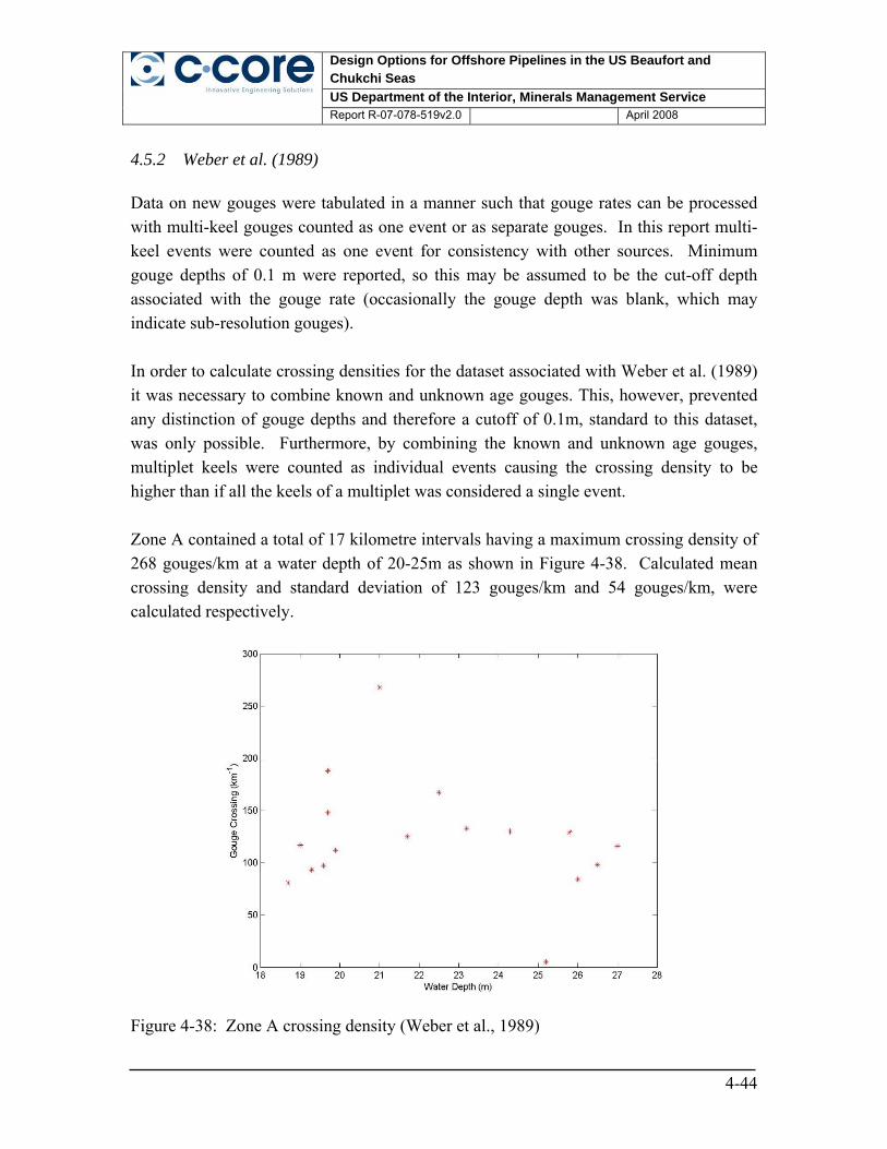
within the zoned areas of the US Beaufort Sea to perform a reliable analysis of gouge geometry (Rearic and McHendrie, 1983 and Weber et al., 1989). Appendix A presents an overview of this data. In addition, more limited data presented in MMS (2002) relating to field surveys at the Northstar and Liberty sites have been reviewed and compared with the USGS dataset. The data associated with Rearic and McHendrie (1983) are a combination of USGS ice gouge data referenced from two separate Alaskan Beaufort Sea surveys; Rearic et al. (1981) and Reimnitz and Kempema (1982a). Recorded ice gouge data include gouge location, water depth, maximum gouge depth, incision width and length. Single and multiplet gouges are described in the data indicating the number of multi-incision gouges; however, only the maximum number of incisions per gouge interval is provided. This does not allow the distinction between single and multiplet events and therefore multi-keel gouges have been counted as single events, rather than considering each gouge comprising the multi-keel gouge as a separate entity. Ice gouge locations are recorded in NAD27 datum geodetic format coordinates. Ice gouge observation statistics and frequencies are recorded within specified ice gouge depth classes for gouge depth ranges from less than 0.4m (0.2m – 0.4m) to less than 4.0m (3.8 - 4.0m) in 0.2m intervals. Figure 4-4 provides the location of track lines associated with this dataset in relation to the specified zones. Weber et al. (1989) contains gouges of known and unknown age and presents results from repetitive mapping surveys collected over the 9 sites shown in Figure 4-5 during 1977 – 1985. The new gouge data are divided into kilometre segments indicating the water depth and total number of gouges of unknown and known age. The age of gouges is determined by identifying new gouges related to the previous survey along a particular track line. Each new gouge interval is further subdivided into single and multiplet gouge events, providing gouge depth and width for single events and number of incisions per multiplet, maximum gouge depth and width for multiplet events. Coordinates were not reported for the 9 sites; however, comparison of water depths and corridors with that of Barnes and Rearic (1985) data allowed confident correlation to be made between surveys. Locations for the 1989 data were therefore inferred using this comparison. Data on new gouges were tabulated in a manner such that gouge rates can be processed with multi-keel gouges counted as 1 event or as separate gouges. In this report multi-keel events were counted as 1 event for consistency with other sources.
Design Options for Offshore Pipelines in the US Beaufort and Chukchi Seas US Department of the Interior, Minerals Management Service
Report R-07-078-519v2.0 April 2008
4-6
Records of 836 ice gouge events, 307 gouges of which had useable gouge depth and width information were included in the MMS (2002) GIS database. Figure 4-6 presents the location of these ice gouges in relation to the defined zones, identifying those gouges with useable geometric data. Useable gouges, with tabulated data related to surveys performed at the Northstar and Liberty Fields, and fall mainly within Zones C and D respectively. The Northstar development lies northwest of Prudhoe Bay and the Liberty development is located in Foggy Island Bay, approximately 2.5km southeast of the Endicott Satellite Island. Figure 4-7 presents a closer view of the ice gouges located in each development. Northstar was surveyed from 1995 to 1998 collecting data on 120 gouges while Liberty was surveyed from 1997 to 1998 collecting 187 gouge events. It is understood that the pipeline route at Northstar is undergoing regular repetitive surveying, but the data have not been made available to this study. It should also be noted that the extent of the various Zones, particularly Zone A, was established using regional bathymetry mapping whereas a more precise spot reading was used to record the depth of each individual kilometre segment in the ice gouge surveys. For this reason, although Zone A is bounded between approximately 20m to 60m contours, it is possible to have a gouge with a water depth less than 20m in this Zone. This also applies to the other zones, for example Zone C includes data in water depths greater than 20m. A summary of the parameters associated with each data set pertaining to the reports Rearic and McHendrie (1983) and Weber et al. (1989) are presented in Table 4-3. A summary of the parameters obtained from the MMS (2002) data is given in Table 4-4.
Design Options for Offshore Pipelines in the US Beaufort and Chukchi Seas US Department of the Interior, Minerals Management Service
Report R-07-078-519v2.0 April 2008
4-7
Zone A
Zone B Zone D
Zone C
Figure 4-4: Rearic and McHendrie (1983) track lines
Zone A
Zone B Zone D
Zone C
12
36
5 & 87
4
9
Figure 4-5: Weber et al. (1989) corridors
Design Options for Offshore Pipelines in the US Beaufort and Chukchi Seas US Department of the Interior, Minerals Management Service
Report R-07-078-519v2.0 April 2008
4-8
Figure 4-6: MMS (2002) GI S database ice gouge locations
Figure 4-7: Ice gouges surveyed adjacent to Northstar and Liberty developments
Design Options for Offshore Pipelines in the US Beaufort and Chukchi Seas US Department of the Interior, Minerals Management Service
Report R-07-078-519v2.0 April 2008
4-9
Table 4-3: Summary of Rearic and McHendrie (1983) and Weber et al. (1989) data sets
Parameter Rearic and
McHendrie (1983) Weber et al. (1989)
Dates surveyed 1972 - 1981 1977 - 1985 Repetitive mapping used? N Y Total no. of km surveyed 2443 316 Total no. of gouges recorded (single keel/multiplet)
132183 19327 (s + m)
Seabed soil type identified? Y N
Gouge depths recorded Y (s/m not
differentiated) Y (new gouges only)
Gouge widths recorded Y (max values per km
segment only) Y (new gouges only)
Zone A Water depth covered 10-60m 15-30m Number of km surveyed 615 16 Total number of gouges recorded * 46885 2091 Number of new gouges recorded (s/m) - 33 / 31
Zone B Water depth covered 0-25m 5-20m Number of km surveyed 117 87 Total number of gouges recorded * 8534 5725 Number of new gouges recorded (s/m) - 254 / 124
Zone C Water depth covered 0-30m 5-25m Number of km surveyed 464 108 Total number of gouges recorded * 22583 2675 Number of new gouges recorded (s/m) - 286 / 88
Zone D Water depth covered 0-10m - Number of km surveyed 377 - Total number of gouges recorded * 1197 - Number of new gouges recorded (s/m) - -
• s/m - single and multiplet gouges only differentiated for new gouges
Design Options for Offshore Pipelines in the US Beaufort and Chukchi Seas US Department of the Interior, Minerals Management Service
Report R-07-078-519v2.0 April 2008
4-10
Table 4-4: Summary of MMS (2002) data sets
Parameter GIS Dates surveyed 1995 - 1998 Repetitive mapping used? Y Total no. of gouges recorded (single keel/multiplet)
836
Seabed soil type identified? N Gouge depths recorded Y Gouge widths recorded Y Northstar Total number of gouges recorded * 120 Liberty Total number of gouges recorded * 187
• Single and multiplet gouges are not differentiated 4.3 Gouge Depth
The gouge depth at a given point along a gouge feature is the distance between the undisturbed seabed and the deepest point in the gouge cross-section at the time of the survey. The assumption is that gouge depths represent random point values obtained in the course of running pre-selected survey lines (which is the usual case), rather than maximum depths measured along full gouge lengths or sections of gouges (i.e. maximum depth recorded in a multibeam swath). It should be noted that gouge surveys may be performed months or years after initial formation of the gouge by ice keels. It is therefore likely that the gouge has had some infilling of sediment between the time of formation and the survey measurement, particularly in shallow water. This is not accounted for in the data as presented in this report, and will affect the reported values of depth distribution, as discussed by Palmer et al. (2005) and Palmer and Niedoroda (2005). Numerical sediment transport models have been developed e.g. Niedoroda and Palmer (1986) which could allow an estimate of infill rates to be determined. Gouge data were analyzed for track lines falling into each Zone A to D, and combined to allow analysis for a range of water depths. The gouge depth distributions were developed
Design Options for Offshore Pipelines in the US Beaufort and Chukchi Seas US Department of the Interior, Minerals Management Service
Report R-07-078-519v2.0 April 2008
4-11
to provide mean and standard deviation values, characterized using the λ parameter, which is the decay coefficient for the exponential distribution. The λ parameter is the reciprocal of the sample mean, corrected for the gouge depth cut-off (i.e. for a mean gouge depth of 0.7 m, with a cut-off of 0.2 m, λ = 1/(0.7-0.2) = 2). This type of distribution was assumed based on previous work by Weeks et al. (1983), although Nessim and Hong (1992) the Canadian Beaufort ice gouge depth data were best represented by a gamma or Weibull distribution. Significantly more data points are required to select an appropriate distribution function. The exponential distribution is selected here for demonstration purposes only. Moreover, the design conditions are controlled by extreme values which may be affected and constrained by processes that do not affect mean conditions. For example, infrequent ice island incursions may generate some of the deeper gouges observed. Conversely, the extreme gouges will be limited in depth by the available environmental driving forces and the maximum ice keel resistance.
Figure 4-8: Fits to samples of exponentially distributed data The goodness of fit of the selected distribution also can not be used to assess whether the appropriate distribution is valid for extreme conditions. Consider two selections of 2000 random samples from a perfect exponential distribution with a mean of 0.4m. Exponential fits to these data, Figure 4-8 provide reasonable means of 0.404m and
Design Options for Offshore Pipelines in the US Beaufort and Chukchi Seas US Department of the Interior, Minerals Management Service
Report R-07-078-519v2.0 April 2008
4-12
0.391m, but the extreme values, beyond 2m depth, would appear to deviate from the selected distribution. The issue of sample size is important and must therefore be considered in assessing design uncertainty. The current analysis was based on the binned number of gouges per 0.2 m gouge depth increment. Gouges with depths <0.2m were not considered. A minimum gouge depth of 0.1 m was reported in Weber et al. (1989), so this may be assumed to be the cut-off depth associated with the gouge rate (occasionally the gouge depth was blank, which may indicate sub-resolution gouges). To perform a comparison of datasets it was necessary for both datasets to have the same cut-off gouge depth. A cut-off limit of 0.2m was therefore established from Rearic and McHendrie (1983) and applied to Weber et al. (1989); however, this severely reduced the number of available data points used in the analysis. 4.3.1 Rearic and McHendrie (1983)
The gouge depths in this dataset were tabulated for intervals of 0.2m in depth. To allow for distributions to be applied and for further analysis, a gouge depth value was selected for each interval; in this case the midpoint of the interval was used. This produced scatter plots that have a banded appearance. It is therefore possible for a gouge depth to be +/- 0.1m of the given value. This method was consistently used throughout the entire dataset.
There were a total of 18,392 gouge depths located within Zone A, ranging in water depth from 10m to 60m. A maximum gouge depth of 3.9m was recorded in 3 occurrences within a water depth range of 30-40m, and a mean for the entire zone of 0.5m with a standard deviation of 0.3m. The gouge depths in this zone follow an exponential distribution with a decay coefficient (λ) of 3.8m-1. A complete summary of the data collected for this zone is located in Figure 4-9 and depth exceedance curves are presented in Figure 4-10 and Figure 4-11 as a function of water depth.
Design Options for Offshore Pipelines in the US Beaufort and Chukchi Seas US Department of the Interior, Minerals Management Service
Report R-07-078-519v2.0 April 2008
4-13
Figure 4-9: Zone A gouge depth summary (Rearic and McHendrie, 1983)
Figure 4-10: Zone A gouge depth exceedance curves 10-35m water depth (Rearic and McHendrie, 1983)
Design Options for Offshore Pipelines in the US Beaufort and Chukchi Seas US Department of the Interior, Minerals Management Service
Report R-07-078-519v2.0 April 2008
4-14
Figure 4-11: Zone A gouge depth exceedance curves 40-60m water depth (Rearic and McHendrie, 1983)
Zone B spanned water depths from 0m to 25m containing 857 gouge depths, and a maximum gouge depth of 1.1m in water 10-15m deep occurring 7 times within the zone. Overall, the mean gouge depth of the zone was 0.4m having a standard deviation of 0.15m. Similar to Zone A, the gouge depths in this zone also can be fitted with an exponential distribution with a decay coefficient (λ) of 5.9m-1. The obvious binning of data into gouge depth intervals is a result of the original presentation of the data in Rearic and McHendrie (1983). A full summary of Zone B is plotted in Figure 4-12, with exceedance curves given in Figure 4-13.
Design Options for Offshore Pipelines in the US Beaufort and Chukchi Seas US Department of the Interior, Minerals Management Service
Report R-07-078-519v2.0 April 2008
4-15
Figure 4-12: Zone B gouge depth summary (Rearic and McHendrie, 1983)
Figure 4-13: Zone B gouge depth exceedance curves (Rearic and McHendrie, 1983)
Design Options for Offshore Pipelines in the US Beaufort and Chukchi Seas US Department of the Interior, Minerals Management Service
Report R-07-078-519v2.0 April 2008
4-16
Zone C, summarized in Figure 4-14, contains 5204 gouge depths ranging in water depths from 0m to 30m. A maximum gouge depth of 1.7m was recorded in water depth of 15m-20m, occurring within 3 different gouges. An average gouge depth of 0.4m was calculated for the zone, with a standard deviation of 0.21m. An exponential distribution can also be fitted to the gouge depths of Zone C, having an exponential decay coefficient (λ) of 4.9m-1. Figure 4-15 presents exceedance curves for Zone C.
Figure 4-14: Zone C gouge depth summary (Rearic and McHendrie, 1983)
Design Options for Offshore Pipelines in the US Beaufort and Chukchi Seas US Department of the Interior, Minerals Management Service
Report R-07-078-519v2.0 April 2008
4-17
Figure 4-15: Zone C gouge depth exceedance curves (Rearic and McHendrie, 1983)
Zone D is subdivided into 2 separate identities labelled Zone D1 and D2. Only 4 data points were recorded for Zone D1, having a maximum gouge depth of 0.5m and an average of 0.35m. There were insufficient points to accurately fit a distribution to this data. Similarly, Zone D2 was limited to only 24 data points ranging in water depths from 0 to 10m. A maximum gouge depth of 0.7m was recorded in 0-5m of water, and a mean value of 0.3m was observed over the entire zone. Likewise, due to the lack of information available, a distribution could not be confidently fitted to the data. Figure 4-16 summarizes both locations, Zone D1 and D2 and Figure 4-17 presents exceedance curves. A complete summary table for Rearic and McHendrie (1983), organized with water depths horizontal and zones vertical, is presented in Table 4-5.
Design Options for Offshore Pipelines in the US Beaufort and Chukchi Seas US Department of the Interior, Minerals Management Service
Report R-07-078-519v2.0 April 2008
4-18
Figure 4-16: Zone D gouge depth summary (Rearic and McHendrie, 1983)
Figure 4-17: Zone D gouge depth exceedance curves (Rearic and McHendrie, 1983)
Design Options for Offshore Pipelines in the US Beaufort and Chukchi Seas US Department of the Interior, Minerals Management Service
Report R-07-078-519v2.0 April 2008
4-19
Table 4-5: Summary of Rearic and McHendrie (1983) Gouge Depths
Design Options for Offshore Pipelines in the US Beaufort and Chukchi Seas US Department of the Interior, Minerals Management Service
Report R-07-078-519v2.0 April 2008
4-20
4.3.2 Weber et al. (1989)
This dataset provides distinction between single and multiplet gouge events for known age gouges only; however, since a gouge depth cutoff of 0.2m was applied, the abundance of data points that fall within each zoned area were greatly reduced. The 9 corridors associated with this dataset are outside the Barrier Islands in the Beaufort Sea and therefore no information was available for Zone D. Only gouges of known age were used in the analysis of Weber et al. (1989). Zone A contained data with water depths ranging from 15-25m for single gouges and 15-30m for multiplet gouges. There were only 6 single gouge events recorded, having a maximum gouge depth of 0.5m in 15-20m of water and an overall mean of 0.3m. A total of 16 multiplets were also located within this zone with a maximum gouge depth of 1.2m and a mean of 0.5m. Although there are only 16 multiplet events, an exponential distribution can be fitted to the data with λ = 3.0m-1. With even fewer single gouges, an exponential distribution can be fitted; however, the confidence level in applying this fit is low and should be considered approximate. These data are plotted in Figure 4-18. .
Figure 4-18: Zone A gouge depth summary - known age (Weber et al., 1989)
Design Options for Offshore Pipelines in the US Beaufort and Chukchi Seas US Department of the Interior, Minerals Management Service
Report R-07-078-519v2.0 April 2008
4-21
Within Zone B there were 27 single gouges and 17 multiplet gouges located in water depth ranges of 5-20m and 10-20m respectively. A maximum single gouge depth of 3m was recorded in a water depth of 10-15m with an overall single mean gouge depth of 0.5m. The maximum gouge depth for the multiplets is much lower having a value of 0.8m in 15-20m water depth. The average depth is similar with a value of 0.4m. An exponential distribution can be fitted to both single and multiplet gouge depths; however, due to the lack of data, the confidence level in applying this fit is somewhat lower. These data are plotted in Figure 4-19.
Figure 4-19: Zone B gouge depth summary – known age (Weber et al., 1989)
A total of 15 single and 5 multiplet gouges were recorded in Zone C within a water depth range of 5-25m. Figure 4-20 illustrates that Zone C had a maximum single gouge depth of 1.4m occurring in water depth 15-20m and a mean single gouge depth of 0.5m. A maximum multiplet gouge depth of 3.0m was found at 10-15m and the average multiplet depth was 0.9m. Although there was an inadequate number of multiplet gouges to fit a distribution, an exponential curve with a decay coefficient of 3.1m-1 for single gouges was derived.
Design Options for Offshore Pipelines in the US Beaufort and Chukchi Seas US Department of the Interior, Minerals Management Service
Report R-07-078-519v2.0 April 2008
4-22
Figure 4-20: Zone C gouge depth summary – known age (Weber et al., 1989)
A complete summary of the data presented in the scatter plots for Weber et al. (1989) is tabulated for single gouges in Table 4-6 and for multiplet gouges in Table 4-7. Figure 4-21 and Figure 4-22 present gouge depth exceedance curves for single and multiple gouge events respectively.
Design Options for Offshore Pipelines in the US Beaufort and Chukchi Seas US Department of the Interior, Minerals Management Service
Report R-07-078-519v2.0 April 2008
4-23
Table 4-6: Single Gouge Depths (Weber et al., 1989)
Design Options for Offshore Pipelines in the US Beaufort and Chukchi Seas US Department of the Interior, Minerals Management Service
Report R-07-078-519v2.0 April 2008
4-24
Figure 4-21: Gouge depth exceedance curves for single keel events (Weber et al., 1989)
Figure 4-22: Gouge depth exceedance curves for multiple keel events (Weber et al., 1989)
Design Options for Offshore Pipelines in the US Beaufort and Chukchi Seas US Department of the Interior, Minerals Management Service
Report R-07-078-519v2.0 April 2008
4-25
4.3.3 MMS (2002)
The gouge depths provided in MMS (2002) were assumed to be the distance between the undisturbed seabed and the deepest point in the gouge, although no details have been provided on the methodology used in the survey. A cutoff depth of 0.2m was applied to allow a direct comparison with the results from the Rearic and McHendrie (1983) and Weber et al. (1989) datasets, although this greatly reduced the amount of data points available, especially for the Liberty survey. 70 gouges were analysed for the Northstar development with measurable gouge depths, resulting in an average depth of 0.3m and a maximum of 0.6m. The gouge depths follow an exponential distribution with an exponential decay coefficient of 9.0m-1, as shown in Figure 4-23.
Design Options for Offshore Pipelines in the US Beaufort and Chukchi Seas US Department of the Interior, Minerals Management Service
Report R-07-078-519v2.0 April 2008
4-26
Application of the 0.2m gouge depth cut-off for the Liberty Field data resulted in a single gouge with a depth of 0.4m. No mean values could therefore be developed. Table 4-8 provides a summary of the data collected for the Northstar and Liberty development areas. No water depth data were provided to directly correlate with gouge geometry, although the surveys were performed in water depths of 5 to 12m at the Northstar and 1.5 to 7m at the Liberty locations.
Table 4-8: Summary of MMS (2002) gouge depths
Figure 4-24: Mean gouge depth comparison of zoned datasets
Design Options for Offshore Pipelines in the US Beaufort and Chukchi Seas US Department of the Interior, Minerals Management Service
Report R-07-078-519v2.0 April 2008
4-27
4.3.4 Comparison of Data and Recommended Gouge Depth Distributions
The mean gouge depth for each water interval was calculated for each dataset and plotted, as shown in Figure 4-24. Mean gouge depth increases with water depth, similar to that seen in Nessim and Hong (1992) for the Canadian Beaufort Sea, with greatest gouge depths in the water depth range of 25-45m. There is no consistent basis on which to base differences between the unknown age gouge depths of Rearic and McHendrie (1983) and the known age gouge depths of Weber et al. (1989). A correlation was derived for the Canadian Beaufort Sea by Nessim and Hong (1992) as shown in Figure 4-25 although additional survey data would be needed to develop a similar approach for the US Beaufort Sea. Such a correlation would take account of sediment infilling as discussed in Section 1. There is also little distinction to be made between gouge depths at the same water depth in different zones. The data obtained from the MMS (2002) database are not plotted on Figure 4-24, but correlates well with the USGS data.
Figure 4-25: Ratio between means of new and existing gouge depths as a function of water depth in Canadian Beaufort Sea (Nessim and Hong, 1992)
Gouges will partially infill to some degree immediately after creation, before they are first surveyed. Infilling will continue with time. Nessim and Hong (1992), Figure 4-25, developed the relationship shown using data collected in the Canadian Beaufort by Canadian Seabed Research (1978 to 1990). “Existing” gouges refers to gouge depths measured during a baseline survey, where there is no indication of the age of a gouge and
Design Options for Offshore Pipelines in the US Beaufort and Chukchi Seas US Department of the Interior, Minerals Management Service
Report R-07-078-519v2.0 April 2008
4-28
the measured depths are a mixture of new and older features. New gouges are gouges identified through subsequent repetitive mapping along baseline surveys. The ratio Figure 4-25 is between the mean depths for the new and existing gouges in each water depth range. The ratio in the 5 to 10 m water depth range is close to zero. According to Nessim and Hong, “this may be an indication that the scouring activity is very high in shallow water, so that most recorded scours in shallow water are relatively new”. What is interesting is that the figure indicates the “existing” gouges in the 5 to 10 water depth range are slightly deeper (about 8%) than the new gouges. This could be a quirk in the data, or possibly deeper gouges are better preserved in a high scour rate regime (shallower gouges more readily obliterated by subsequent gouging). For comparison, in 5 – 10m water depth range there were 1,064 new gouges (mean depth 0.217 m, standard deviation 0.170 m) and 825 existing gouges (mean depth 0.235 m, standard deviation 0.345 m). In deeper water the trend is as expected – new gouges are deeper, peaking at the 20-25 m depth range with a ratio of 1.32 against existing gouges. 4.4 Gouge Width
While deeper gouges tend to be wider, wide gouges are not necessarily deep. Accurately defining the joint distribution of gouge width and depth requires significantly more data than are available at this time. Early analyses focused on the gouge depth distribution, and the gouge width distribution was considered of secondary importance. Often gouge widths were not reported (i.e. Weeks et al., 1983), or only maximum gouge widths were noted (i.e. Rearic and McHendrie, 1983). Gouges are classified as single keel or multi-keel features. The common conception of multi-keel gouge formation is a rake-like arrangement of keels that simultaneously crosses an area, and some multi-keel gouges can be well in excess of 100 meters in width. It is possible that multi-keel gouges may be more accurately considered as a series of superimposed single keel gouges. The keels may be embedded in the same ice floe, so resulting gouges would have the same orientation (due to the floe motion), but depend on alignment of the ridge with the driving forces. The implication is that using a gouge width distribution that includes multi-keel gouge widths may overestimate the mean gouge width and produce a distorted distribution. Another consideration is that multi-keel gouges are not necessarily continuous over the gouge width and can have undisturbed sediment within the recorded gouge width. Again, the “effective” gouge width would be less than the measured width. While the second issue (effective gouge width) could be addressed by the analyses of scour records, the first issue (simultaneous
Design Options for Offshore Pipelines in the US Beaufort and Chukchi Seas US Department of the Interior, Minerals Management Service
Report R-07-078-519v2.0 April 2008
4-29
vs. non-simultaneous multi-keel gouge formation) may never be able to be addressed satisfactorily. Comparisons in data measurement for single and multi-keel events are illustrated in Figure 4-26. Based on the points discussed above, the actual gouge width is likely to be narrower than the measured gouge width (based on the overall population), thus the sensitivity case to be considered would be a narrower gouge width distribution. An additional point that must be considered is whether the reported gouge width was measured from the berm-to-berm gouge width (distance between tops of berms, readily extracted from side scan records) or the incision gouge width (the width of the actual incision formed in the seabed), shown as variable w in Figure 4-26. The incision width is narrower than the berm-to-berm tip width, and is the correct parameter to use, but it is not always clear how reported widths were measured. 4.4.1 Rearic and McHendrie (1983)
The dataset provided with the Rearic and McHendrie (1983) report only tabulated the maximum gouge width for each kilometre segment and no distinction of whether this measurement was from a single or a multiplet gouge was given. No apparent conclusions or distributions can, therefore, be produced from this dataset. 4.4.2 Weber et al. (1989)
In this dataset it should be noted that single gouge widths are defined as the cross-sectional distance across the trough at the undisturbed seabed level and multiplet gouge widths are the total disturbed width at the undisturbed seabed level, as shown in Figure 4-26.
Design Options for Offshore Pipelines in the US Beaufort and Chukchi Seas US Department of the Interior, Minerals Management Service
Report R-07-078-519v2.0 April 2008
4-30
Figure 4-26: Diagram of Typical Ice Gouge Measurements Presented Within USGS Open-File Report 81-950 (Rearic et al., 1981).
In Zone A, 6 single gouge and 16 multiplet gouge widths were measured in water depths of 15-30m. A maximum singe gouge width of 5m was measured between 20-25m, having a zone mean of 3m and a standard deviation of 1m. Likewise, a maximum multiplet gouge width of 132m was measured at a water depth of 20-25m and an overall mean width of 39m with a standard deviation of 34m. Unlike gouge depths, gouge widths follow more of a lognormal distribution; however, due to the lack of data points, the distribution match is not definitive. The data for Zone A are presented in Figure 4-27.
Design Options for Offshore Pipelines in the US Beaufort and Chukchi Seas US Department of the Interior, Minerals Management Service
Report R-07-078-519v2.0 April 2008
4-31
Figure 4-27: Zone A gouge width summary for single and multiplet gouges (Weber et al., 1989)
Zone B contains water depths of 5-20m with 27 single gouges and 17 multiplets, Figure 4-28. A maximum single gouge width of 22m was measured at a water depth of 10-15m, and a total zone mean and standard deviation of 6m and 4m, respectively, was calculated. Similarly, a maximum multiplet gouge width of 60m was observed at a water depth of 10-15m and an overall mean of 23m and standard deviation of 13m was calculated. Although the number of data points were limited, a lognormal distribution can be fitted to the data.
Design Options for Offshore Pipelines in the US Beaufort and Chukchi Seas US Department of the Interior, Minerals Management Service
Report R-07-078-519v2.0 April 2008
4-32
Figure 4-28: Zone B gouge width summary for single and multiplet gouges (Weber et al., 1989)
For the 5-25m water depth range, 15 single and 5 multiplet gouge widths were recorded for Zone C. A maximum gouge width of 20m was reported for single gouges at a water depth of 15-20m, with a zone mean of 6m and standard deviation of 4m. A maximum multiplet gouge width of 57m was also reported at a water depth of 15-20m, with a mean width for Zone C of 31m and a standard deviation of 24m. Again, due to a lack of data points it is difficult to fit a distribution with high confidence; however, with the widths provided, a lognormal distribution appears to provide a good fit. All the data associated with Zone C can be located in Figure 4-29.
Design Options for Offshore Pipelines in the US Beaufort and Chukchi Seas US Department of the Interior, Minerals Management Service
Report R-07-078-519v2.0 April 2008
4-33
Figure 4-29: Zone C gouge width summary for single and multiplet gouges (Weber et al., 1989)
A number of outlying data points are evident in each zone, particularly with respect to multiplet gouges. This can have a significant effect on soil deformations below the gouge and adds to the uncertainty regarding data interpretation. A complete summary of the data presented in the gouge width scatter plots for Weber et al. (1989) is tabulated for single gouges in Table 4-9 and for multiplet gouges in Table 4-10. Figure 4-30 and Figure 4-31 present gouge width exceedance curves for single and multiple events respectively.
Design Options for Offshore Pipelines in the US Beaufort and Chukchi Seas US Department of the Interior, Minerals Management Service
Report R-07-078-519v2.0 April 2008
4-34
Table 4-9: Single gouge widths (Weber et al., 1989)
Design Options for Offshore Pipelines in the US Beaufort and Chukchi Seas US Department of the Interior, Minerals Management Service
Report R-07-078-519v2.0 April 2008
4-35
Figure 4-30: Gouge width exceedance curves (Weber et al., 1989)
Figure 4-31: Gouge width exceedance curves (Weber et al., 1989)
Design Options for Offshore Pipelines in the US Beaufort and Chukchi Seas US Department of the Interior, Minerals Management Service
Report R-07-078-519v2.0 April 2008
4-36
4.4.3 MMS (2002)
Gouge width data were analysed for gouges having depths greater than 0.2m, to allow consistent comparison with the USGS data. A total of 70 gouge widths were analysed for the Northstar development resulting in a mean width of 8m and a maximum width of 36m. From Figure 4-32, a lognormal distribution can be fitted to the Northstar widths, although this data are of limited use since single and multiplet gouges were not differentiated. The lognormal fit lies below the data and suggests that gouge widths will be somewhat underestimated using this approach. A single gouge width of 9m was collected for the Liberty development. Table 4-11 provides a summary of the data collected for the Northstar and Liberty development areas.
Design Options for Offshore Pipelines in the US Beaufort and Chukchi Seas US Department of the Interior, Minerals Management Service
Report R-07-078-519v2.0 April 2008
4-37
Table 4-11: Summary of MMS (2002) gouge widths
4.4.4 Comparison of Data and Recommended Gouge Width Distributions
As mentioned previously, Rearic and McHendrie (1983) did not report any individual gouge widths and therefore it is not possible to make a comparison to the new gouge widths in Weber et al. (1989). A summary plot of the mean gouge widths for Weber et al. (1989) is, however, given in Figure 4-33. This plot shows a general tread of gouge width increases with water depth for both single and multiplet gouges. The MMS (2002) data falls within the range given by the USGS dataset.
Figure 4-33: Mean gouge width comparison of zoned datasets
Northstar Liberty All No. 70 1 71
Mean (m) 8 9 8 Max (m) 36 9 36 Std (m) 7 - 7
Design Options for Offshore Pipelines in the US Beaufort and Chukchi Seas US Department of the Interior, Minerals Management Service
Report R-07-078-519v2.0 April 2008
4-38
4.5 Crossing Density
Surveys of gouges of unknown age (as a result of survey lines only being surveyed once) allow a crossing density to be estimated. Consideration of the gouge signature and its level of degradation can in some cases also be used to estimate formation rates. It is beneficial to develop a crossing density (km-1), which can then be compared to crossing rates of known age gouges in similar geographical locations to develop a correlation between crossing density (km-1) and crossing frequency (km-1yr-1) to be established. A comparison can only be made however, if it is assumed that the gouge infill and erosion is small over the long term, which may not be the case in all areas. 4.5.1 Rearic and McHendrie (1983)
This dataset provides gouges of unknown age which does not allow calculation of crossing frequency. A crossing density (km-1) was therefore calculated for each kilometre segment within each Zone. Zone A contained a total of 498 kilometre length intervals with a maximum crossing density of 147 gouges/km in a water interval of 20-25m. There was an average of 37 gouges/km for the entire zone having a standard deviation of 35 gouges/km. A complete summary of the crossing density for Zone A can be found in Figure 4-34.
Design Options for Offshore Pipelines in the US Beaufort and Chukchi Seas US Department of the Interior, Minerals Management Service
Report R-07-078-519v2.0 April 2008
4-39
Figure 4-34: Zone A crossing density (Rearic and McHendrie 1983)
There were 144 kilometre intervals recorded for Zone B with a maximum crossing density of 65 gouges in a water depth of 15-20m. An average of 6 gouges/km and a standard deviation of 9 gouges/km were calculated for Zone B. Figure 4-35 plots the crossing rates for each water depth interval for Zone B, and shows that crossing density increases with increasing water depth.
Design Options for Offshore Pipelines in the US Beaufort and Chukchi Seas US Department of the Interior, Minerals Management Service
Report R-07-078-519v2.0 April 2008
4-40
Figure 4-35: Zone B crossing density (Rearic and McHendrie 1983)
Zone C contained 391 kilometre intervals with a maximum crossing density of 129 gouges/km in the water depth range of 20-25m. An average crossing density of 13 gouges/km and a standard deviation of 24 gouges/km was also calculated. It can be seen from Figure 4-36 that the crossing density increases with water depth up to the 20-25m water depth limit of this zone, in a similar manner to that of Zone B. The crossing rate then appears to decrease in deeper water as seen in Figure 4-34 for zone A.
Design Options for Offshore Pipelines in the US Beaufort and Chukchi Seas US Department of the Interior, Minerals Management Service
Report R-07-078-519v2.0 April 2008
4-41
Figure 4-36: Zone C crossing density (Rearic and McHendrie 1983)
Zone D1 recorded 68 kilometre intervals with a maximum of 2 gouges in 0-5m water depth with a mean of 0.1 gouges/km and a standard deviation of 0.3 gouges/km. Zone D2 contained 286 kilometre intervals with a maximum of 4 gouges per km with a mean crossing density of 0.1 and a standard deviation of 0.4. Figure 4-37 provides a summary of Zone D.
Design Options for Offshore Pipelines in the US Beaufort and Chukchi Seas US Department of the Interior, Minerals Management Service
Report R-07-078-519v2.0 April 2008
4-42
Figure 4-37: Zone D crossing density (Rearic and McHendrie 1983)
A complete summary table for the crossing densities of Rearic and McHendrie (1983), organized as a function of water depth and zones, is presented in Table 4-12.
Design Options for Offshore Pipelines in the US Beaufort and Chukchi Seas US Department of the Interior, Minerals Management Service
Report R-07-078-519v2.0 April 2008
4-43
Table 4-12: Summary of Rearic and McHendrie (1983) gouge crossing density
Design Options for Offshore Pipelines in the US Beaufort and Chukchi Seas US Department of the Interior, Minerals Management Service
Report R-07-078-519v2.0 April 2008
4-44
4.5.2 Weber et al. (1989)
Data on new gouges were tabulated in a manner such that gouge rates can be processed with multi-keel gouges counted as one event or as separate gouges. In this report multi-keel events were counted as one event for consistency with other sources. Minimum gouge depths of 0.1 m were reported, so this may be assumed to be the cut-off depth associated with the gouge rate (occasionally the gouge depth was blank, which may indicate sub-resolution gouges). In order to calculate crossing densities for the dataset associated with Weber et al. (1989) it was necessary to combine known and unknown age gouges. This, however, prevented any distinction of gouge depths and therefore a cutoff of 0.1m, standard to this dataset, was only possible. Furthermore, by combining the known and unknown age gouges, multiplet keels were counted as individual events causing the crossing density to be higher than if all the keels of a multiplet was considered a single event. Zone A contained a total of 17 kilometre intervals having a maximum crossing density of 268 gouges/km at a water depth of 20-25m as shown in Figure 4-38. Calculated mean crossing density and standard deviation of 123 gouges/km and 54 gouges/km, were calculated respectively.
Figure 4-38: Zone A crossing density (Weber et al., 1989)
Design Options for Offshore Pipelines in the US Beaufort and Chukchi Seas US Department of the Interior, Minerals Management Service
Report R-07-078-519v2.0 April 2008
4-45
87 kilometre intervals were recorded in Zone B with a maximum crossing density of 171 gouges/km at a water depth of 10-15m. An average crossing density of 66 gouges/km and a standard deviation of 40 gouges/km was also calculated for the entire zone, shown in Figure 4-39, although there seems to be a strong correlation between crossing density and water depth.
Figure 4-39: Zone B crossing density (Weber et al., 1989)
Zone C consisted of 107 kilometre intervals with a maximum crossing density of 132 gouges/km recorded at a water depth of 15-20m. Also calculated were a mean of 24 gouges/km and a standard deviation of 29 gouges/km, although a correlation between crossing density and water depth was again observed. Figure 4-40 is a plot summary of crossing density versus water depth for Zone C. A complete summary table for the crossing densities of Weber et al. (1989), organized with water depths horizontal and zones vertical, is given in Table 4-13.
Design Options for Offshore Pipelines in the US Beaufort and Chukchi Seas US Department of the Interior, Minerals Management Service
Report R-07-078-519v2.0 April 2008
4-46
Figure 4-40: Zone C crossing density (Weber et al., 1989)
Design Options for Offshore Pipelines in the US Beaufort and Chukchi Seas US Department of the Interior, Minerals Management Service
Report R-07-078-519v2.0 April 2008
4-47
Table 4-13: Summary of Weber et al. (1989) gouge crossing density
No crossing density or frequency was derived from the MMS (2002) data. 4.5.4 Comparison of Crossing Density Datasets
A direct comparison of the crossing densities for Rearic and McHendrie (1983) and Weber et al. (1989) is not possible due to the constraints associated with the original datasets. Rearic and McHendrie (1983) uses a gouge depth cutoff of 0.2m, whereas Weber et al. (1989) uses 0.1m, and since gouge depths are only provided for known age gouges, a combination of known and unknown gouges prevents any adjustments in the cutoff. Rearic and McHendrie (1983) also counted all the keels of a multiplet as a single event, whereas with the combination of known and unknown gouges of Weber et al. (1989), each keel of a multiplet is counted as an individual event. These two differences can lead to an over-estimation of the number of gouges present in each zone. Both datasets can provide useful estimates of crossing rates.
Design Options for Offshore Pipelines in the US Beaufort and Chukchi Seas US Department of the Interior, Minerals Management Service
Report R-07-078-519v2.0 April 2008
4-48
4.6 Crossing Frequencies
The formation rate of ice gouges is typically inferred from repetitive mapping of the seabed. Repetitive mapping consists of comparing surveys of the same portion of the seabed conducted at least one year apart so that new gouges can be identified. In the Beaufort Sea these surveys usually consist of long lines of limited lateral extent, thus the formation rate of gouges is expressed in terms of the number of gouge crossings per unit distance of survey line per unit time (i.e. km-1yr-1). Caution must be exercised when using gouge rates and depths reported in this type of analysis. One example concerns the treatment of single keel and multi-keel (or multiplet) gouges. In most analyses multi-keel gouges were counted as single events, rather than considering each gouge comprising the multi-keel gouge as a separate entity. In order to maintain consistency, the gouge geometry (in particular the gouge depth distribution) should reflect this grouping of gouges into a single event. Thus the maximum gouge depth would be the deepest of all the gouges in the multi-keel event. Assigning the appropriate gouge width can present a challenge since gouges comprising multi-keel events can be separated by appreciable distances – in excess of 100 meters (CSR, 2006). When interpreting gouge rates or comparing gouges rates from different sources care must be exercised that the gouge rate and gouge geometry are consistent. Gouge crossing rates may exclude gouges below a certain threshold (i.e. typically 0.1-0.2 m), or may in some cases include gouge events with depths less than the resolution of the depth profiler. While these sub-resolution gouges may be left out of the gouge depth distribution (resulting in higher mean gouge depths), they may be included in the gouge rate (Nessim and Hong, 1992). Another example concerns the treatment of single keel and multi-keel gouges. In most analyses multi-keel gouges were counted as single events, rather than considering each gouge comprising the multi-keel gouge as a separate entity. In the absence of repetitive mapping, formation rates can be estimated from the appearance of gouges on the seafloor. The gouge age can be estimated from the degree of degradation of the gouge signature. This technique was adopted for the proposed Millennium pipeline crossing, Lever 1999).
Design Options for Offshore Pipelines in the US Beaufort and Chukchi Seas US Department of the Interior, Minerals Management Service
Report R-07-078-519v2.0 April 2008
4-49
4.6.1 Rearic and McHendrie (1983)
This dataset only consists of unknown age gouges and therefore is not possible to calculate a crossing rate frequency. 4.6.2 Weber et al. (1989)
Crossing frequencies for Weber et al. (1989) was obtained through repetitive mapping in the American Beaufort Sea in the period of 1977-1985 using only gouges of known age and with gouge depths greater than 0.2m and counting each multi-keel gouge as a single event. Zone A only contained 2 repetitively mapped kilometre intervals having crossing frequencies of about 1 gouge/km/year in a water depth of 15-20m. Zone B contained 83 repetitively mapped intervals in which a maximum crossing frequency of 3 gouges/km/year was recorded in a water depth of 10-15m as shown in shown in Figure 4-41. An overall zone crossing frequency mean and standard deviation was calculated as 0.5 gouges/km/year and 0.8 gouges/km/year, respectively. The majority of the survey segments were 1km long, such that the data are binned and presented in whole numbers only as an artefact of the data collection process.
Design Options for Offshore Pipelines in the US Beaufort and Chukchi Seas US Department of the Interior, Minerals Management Service
Report R-07-078-519v2.0 April 2008
4-50
Figure 4-41: Zone B crossing frequency (Weber et al., 1989)
A total of 81 repetitively mapped kilometre intervals were recorded for Zone C with a maximum crossing frequency of 6 gouges/km/year in a water depth of 15-20m as shown in Figure 4-42. A mean of 0.2 gouges/km/year and a standard deviation of 0.8 gouges/km/year was calculated for this zone.
Design Options for Offshore Pipelines in the US Beaufort and Chukchi Seas US Department of the Interior, Minerals Management Service
Report R-07-078-519v2.0 April 2008
4-51
Figure 4-42: Zone C crossing frequency (Weber et al., 1989)
A complete summary table for the crossing frequencies of Weber et al. (1989), as a function of water depth and zone, is given in Table 4-14.
Table 4-14: Summary of Weber et al. (1989) gouge crossing frequencies
Design Options for Offshore Pipelines in the US Beaufort and Chukchi Seas US Department of the Interior, Minerals Management Service
A comparison of crossing frequencies between Rearic and McHendrie (1983) and Weber et al. (1989) is not possible since Rearic and McHendrie (1983) does not contain repetitively mapped intervals, necessary to calculate crossing frequencies.
Design Options for Offshore Pipelines in the US Beaufort and Chukchi Seas US Department of the Interior, Minerals Management Service
Report R-07-078-519v2.0 April 2008
5-1
5 CHUKCHI SEA - ICE GOUGING
Ice gouge survey data in the Chukchi Sea are sparse, although the available data allows an assessment of gouge geometry (depth and width), and density to be determined. No repetitive mapping has been performed, and so the age of the observed gouges are unknown and gouging rates cannot be established. To provide a better understanding of gouge characteristics, the Chukchi Sea has been subdivided into representative zones based on differences in environmental conditions, such as hazard regime, which were further divided into water depth intervals. Three zones have been identified in the Chukchi Sea, which present significant differences in conditions, as discussed below:
• Zone A – main shelf area with water depth between 30m and 60m, with bedrock present at shallow depths. Surficial sediments are generally sand and gravel, although these thin deposits overlay stiff consolidated clay or dense sandy gravel within the likely pipeline burial depth. Ice gouging is significant in this zone.
• Zone B – a sub-set of Zone A to the eastern side of the two prominent shoals – the Herald and Hanna shoals. These shoals rise up from the surrounding sea floor having a bathymetry of 40m to a maximum height of 25m, providing some shielding of the seabed from ice ridge keels due to the dominant ice flow direction from west to east. Conversely, an increased ice gouging intensity would be expected on the western flank of the shoals, but the lack of any data in these areas prevents such analysis to be performed.
• Zone C – near shore shallow water below 30m water depth, in which the rate of ice gouging may be lower. Seabed soils consist mainly of gravel deposits.
Figure 5-1 presents a location map of the zones described, and Table 5-1 provides a summary of environmental conditions expected within each zone, including the relative expected frequency of ice gouging and strudel scour. The zoned areas are the main focus of this analysis and data have been analyzed based on these geographical areas.
Design Options for Offshore Pipelines in the US Beaufort and Chukchi Seas US Department of the Interior, Minerals Management Service
Report R-07-078-519v2.0 April 2008
5-2
Figure 5-1: Chukchi Sea case study zones
Table 5-1: Environmental parameters for Chukchi Sea case study zones
Zone Soil Type Ice Gouging Freq. Strudel Scour Freq.
A Stiff clay 100kPa to 200kPa and dense sand 40 to 45°
High Low
B Stiff clay 100 to 200kPa and dense sand 40 to 45°
Low to medium Low
C Dense sand and gravel 40 to 45°
Medium Medium
Design Options for Offshore Pipelines in the US Beaufort and Chukchi Seas US Department of the Interior, Minerals Management Service
Report R-07-078-519v2.0 April 2008
5-3
5.1 Data Sets
Ice gouge data for 10,200 individual ice gouge observations were tabulated by Toimil (1978) within the zoned areas of the Chukchi Sea to perform a reliable analysis of gouge geometry. Appendix B presents an overview of the available data for this region. Recorded ice gouge data includes the observation date, time, ship speed and course, gouges observed, maximum gouge depth, and maximum gouge width. A total of 83 separate tracklines were surveyed, with the geodetic coordinates of the start and end points given. A calculation using the time, ship speed and course, and spherical geometry was necessary to determine the coordinates of each 1 km linear segments which was then used to associate each segment to a zoned area. No distinction between single and multiplet gouges was provided; therefore multi-keel gouges were counted as single events rather than considering each gouge comprising the multi-keel gouge as a separate entity. The recorded maximum ice gouge depth measurements have a resolution of 0.5m, which leads to a high level of inaccuracy when interpreting depth distributions. Figure 5-2 provides the location of track lines associated with this dataset in relation to the specified zones. This dataset does not include repetitive mapping, precluding the calculation of a crossing rates for the zoned areas.
Design Options for Offshore Pipelines in the US Beaufort and Chukchi Seas US Department of the Interior, Minerals Management Service
Report R-07-078-519v2.0 April 2008
5-4
Figure 5-2: Toimil (1978) track lines
Zones were created by overlaying regional bathymetry onto the Chukchi Sea coastline. Water depths associated with Toimil (1978) are site specific and are more accurate than regional bathymetry, therefore it is not uncommon to have a gouge located in a zone but have a water depth beyond the bounded depths of the zone. This can be seen, for example, in Zone C where the zone is bounded by 30m or less water depth but have gouge depths located in 60m of water specifically around the Borrow Valley channel where the seabed gradient rapidly increases. A summary of the parameters associated with the data set pertaining to the Toimil (1978) report are presented in Table 5-2.
Design Options for Offshore Pipelines in the US Beaufort and Chukchi Seas US Department of the Interior, Minerals Management Service
Report R-07-078-519v2.0 April 2008
5-5
Table 5-2: Summary of data set used in study
Parameter Toimil (1978) Dates surveyed 1974 Repetitive mapping used? N Total no. of km surveyed 1364 Total no. of gouges recorded * 10436 Seabed soil type identified? N Gouge depths recorded 584 Gouge widths recorded 245 Zone A Water depth covered 20-75m Number of km surveyed 415 Total number of gouges recorded * 2825 Zone B Water depth covered 25-50m Number of km surveyed 26 Total number of gouges recorded * 6 Zone C Water depth covered 20-110m Number of km surveyed 562 Total number of gouges recorded * 6522
* No distinction between single and multiplet gouges
Design Options for Offshore Pipelines in the US Beaufort and Chukchi Seas US Department of the Interior, Minerals Management Service
Report R-07-078-519v2.0 April 2008
5-6
A secondary source of ice gouge data were provided by Fugro-McClelland Marine Geosciences Inc. and Dames & Moores through the use of high-resolution geophysical surveys. The data provided by these surveys were insufficient to calculate ice gouge depth and widths distributions. Data were provided for 12 prospective drill sites summarized in Table 5-3 for the years 1989 and 1990. Figure 1-1 presents the location of each site in relation to the Alaskan Chukchi Sea coastline.
Table 5-3: Chukchi Sea geophysical surveys
Prospect Lease No. Date Reference
Diamond OCS-Y-0995 1990 No report found Popcorn OCS-Y-1275 1989 Campbell & Rosendahl (1990) Azurite OCS-Y-1279 1989 Nash & Hasen (1990a)
Crackerjack OCS-Y-1312 1989 Taylor & Rosendahl (1990) Dames & Moore (1989a)
Design Options for Offshore Pipelines in the US Beaufort and Chukchi Seas US Department of the Interior, Minerals Management Service
Report R-07-078-519v2.0 April 2008
5-7
Figure 5-3: Completed geo-hazard site specific surveys for the Chukchi Sea OCS waters
Design Options for Offshore Pipelines in the US Beaufort and Chukchi Seas US Department of the Interior, Minerals Management Service
Report R-07-078-519v2.0 April 2008
5-8
Using a combination of echo sounder, side-scan sonar, sub-bottom profiler, mini-sparker, and sparker, various geological conditions were reviewed for each site area, such as:
• Water depth and seafloor topography o Velocity information o Ice gouges – the maximum relief and gouge depth was provided for each
region, along with the average relief, ridge heights, and gouge widths. • Shallow sediments • Buried channels • Shallow structural geology • Shallow gas • Permafrost – it is stated for each prospective drill site that there is no evidence on
any of the seismic data that would suggest the presence of subsea permafrost. Also based on theoretical considerations for water depth, permafrost is unlikely.
• Seismicity – for each prospective drill site the Alaskan Chukchi Shelf has been historically aseismic, and earthquakes are not expected to pose any hazard to exploratory drilling operations.
• Other conditions Each prospective drill site contained information on the above parameters, including a bathymetry and seafloor features map. Figure 5-4 shows an example of the Popcorn Prospect taken from Campbell & Rosendahl (1990). This map indicates water depth contours (solid bold lines), possible seafloor debris, and ice gouges with maximum relief of 2 feet or greater (double line). Numerous shallow or partly buried gouges with relief less than 2 feet could possibly be within this area; however, they are not indicated on this map. With the ice gouge information presented in the bathymetry and seafloor features map, it may be possible to calculate crossing rates and ice gouge depth and width distributions.
Design Options for Offshore Pipelines in the US Beaufort and Chukchi Seas US Department of the Interior, Minerals Management Service
Report R-07-078-519v2.0 April 2008
5-9
Figure 5-4: Example of bathymetry and seafloor features map for plate 3 of the Popcorn Prospect (Campbell and Rosendahl, 1990)
Design Options for Offshore Pipelines in the US Beaufort and Chukchi Seas US Department of the Interior, Minerals Management Service
Report R-07-078-519v2.0 April 2008
5-10
5.2 Gouge Depth
The gouge depth at a given point along a gouge feature is the distance between the undisturbed seabed and the deepest point in the gouge. The gouge depths recorded in Toimil (1978) represent the maximum gouge depths that occur in each segment. Gouge data were analyzed for track lines falling into Zones A to C, and combined to allow analysis for a range of water depths. The gouge depth distributions were developed to provide mean and standard deviation values. There were no gouge depths recorded in water depths greater than 60m. There were a total of 219 gouge depths located within Zone A ranging in water depth from 20m to 50m. A maximum gouge depth of 4.5m was recorded within a water depth of 35-40m, with a mean and standard deviation for the entire zone of 0.8m and 0.6m, respectively. The gouge depths in this zone are seen to follow a lognormal distribution since only maximum gouge depths for each kilometre interval were recorded. Repeatedly sampling the maximum values of an exponential distribution can be shown to give a lognormal fit. A complete summary of the data collected for this zone is given in Figure 5-5. Figure 5-6 presents the gouge depth exceedance curve for Zone A, although there is insufficient data to define these with any level of confidence.
Figure 5-5: Zone A maximum gouge depth summary (Toimil 1978)
Design Options for Offshore Pipelines in the US Beaufort and Chukchi Seas US Department of the Interior, Minerals Management Service
Report R-07-078-519v2.0 April 2008
5-11
Figure 5-6: Zone A gouge depth exceedance curve (Toimil 1978)
Zone B contained a total of 5 track lines, however, no gouge depths were recorded. These lines were of limited length and only in the western half of zone B. Any gouges on the eastern half were not surveyed.
Zone C, summarized in Figure 5-7, contains 275 gouge depths ranging in water depths from 20m to 60m. A maximum gouge depth of 5.0m was recorded in water depth of 30m-35m. An average gouge depth of 0.8m was calculated for the zone, with a standard deviation of 0.4m. A lognormal distribution can also be fitted to the gouge depths of Zone C, similar to that of Zone A, although again, lack of data limits its usefulness. Figure 5-8 presents the depth exceedance curve for Zone C.
Design Options for Offshore Pipelines in the US Beaufort and Chukchi Seas US Department of the Interior, Minerals Management Service
Report R-07-078-519v2.0 April 2008
5-12
Figure 5-7: Zone C max gouge depth summary (Toimil 1978)
Figure 5-8: Zone C gouge depth exceedance curves (Toimil 1978)
Design Options for Offshore Pipelines in the US Beaufort and Chukchi Seas US Department of the Interior, Minerals Management Service
Report R-07-078-519v2.0 April 2008
5-13
A complete summary table for Toimil (1978), organized with water depths horizontal and zones vertical, is illustrated in Table 5-4.
Table 5-4: Summary of Toimil (1978) gouge depths
A B C ALLNo. Gouges 2 34 36Mean (m) 0.8 0.7 0.7Max (m) 1.0 1.0 1.0Std (m) 0.4 0.2 0.2
Accurately defining the joint distribution of gouge width and depth requires significantly more data than are available at this time. Early surveys focused on the gouge depth distribution, and the gouge width distribution was considered of secondary importance. In this dataset, only maximum gouge widths were noted.
Design Options for Offshore Pipelines in the US Beaufort and Chukchi Seas US Department of the Interior, Minerals Management Service
Report R-07-078-519v2.0 April 2008
5-14
The dataset provided with the Toimil (1978) report only tabulated the maximum gouge width for each segment and no distinction of whether this measurement was from a single or a multiplet gouge was given. It is therefore difficult to determine if the maximum gouge widths are defined as either the cross-sectional distance across a single trough at the undisturbed seabed level or the total disturbed width at the undisturbed seabed level as for multiplet gouges. In Zone A, 86 gouge widths were measured in water depths of 25-50m. A maximum gouge width of 95m was measured between 35-40m as shown in Figure 5-9, with a zone mean of 32m and a standard deviation of 22m. Similar to gouge depths, gouge widths follow more of a lognormal distribution; however, due to the lack of data points; the distribution match is not definitive. No exceedance curves were generated, as these data do not allow a meaningful distribution to be developed when only maximum widths for all gouges within a segment were recorded by the surveys.
Figure 5-9: Zone A maximum gouge width summary (Toimil 1978)
Zone B contained a total of 5 track lines, but no gouge widths were recorded.
Design Options for Offshore Pipelines in the US Beaufort and Chukchi Seas US Department of the Interior, Minerals Management Service
Report R-07-078-519v2.0 April 2008
5-15
From 20-55m water depth, 128 gouge widths were recorded for Zone C. A maximum gouge width of 60m occurred 3 times at a water depth of 25-45m, with a zone mean of 14m and standard deviation of 11m. Again, due to a lack of data points it is difficult to fit a distribution with high confidence; however, with the widths provided, a lognormal distribution fits best. All the data associated with Zone C can be located in Figure 5-10.
A complete summary of the data presented in the gouge width scatter plots for Toimil (1978) is presented in Table 5-5.
Figure 5-10: Zone C maximum gouge width summary (Toimil 1978)
Design Options for Offshore Pipelines in the US Beaufort and Chukchi Seas US Department of the Interior, Minerals Management Service
Report R-07-078-519v2.0 April 2008
5-16
Table 5-5: Summary of Toimil (1978) gouge depths
A B C ALLNo. Gouges 14 14Mean (m) 12 12Max (m) 30 30Std (m) 8 8
Design Options for Offshore Pipelines in the US Beaufort and Chukchi Seas US Department of the Interior, Minerals Management Service
Report R-07-078-519v2.0 April 2008
5-17
5.4 Crossing Density
The data presented in Toimil (1978) covers survey lines that were surveyed only once, and so identifies gouges of unknown age, which does not allow calculation of crossing frequency. A crossing density (km-1) was therefore calculated for each segment within Zones A to C. Several segments did not have a water depth associated with them, although a geographical location was presented. These segments were sorted into zones, assigned a water depth of ‘unknown’ and included in the crossing rate calculations. Zone A contained a total of 382 intervals with a maximum crossing rate of 140 gouges in a water interval of 25-30m. There was an average of 7 gouges/km for the entire zone having a standard deviation of 16 gouges/km. A complete summary of the crossing rates for Zone A can be found in Figure 5-11. The crossing density decreases with increasing water depths beyond 30m, then becomes approximately constant to 50m. The crossing density reduces to practically zero in water depths greater than 50m.
Figure 5-11: Zone A crossing rates (Toimil 1978)
There were 21 intervals recorded for Zone B with a maximum crossing rate of 3 gouges/km. Insufficient water depth data were recorded along the survey tracks within
Design Options for Offshore Pipelines in the US Beaufort and Chukchi Seas US Department of the Interior, Minerals Management Service
Report R-07-078-519v2.0 April 2008
5-18
this zone, preventing a correlation to be developed. An average of 0.3 gouges/km and a standard deviation of 0.8 gouges/km were calculated for Zone B. A plot has not been presented for this zone since only one water depth was recorded, associated with 4 segments with gouge crossing rates of zero. The mean crossing rate for Zone B is much lower compared to the other zones. This suggests that the drift direction of the ice from west to east plays a large factor in the amount of ice gouges present. This is further supported by considering 2 track lines located on the west side of the Herald Bank (see Figure 5-2), to the west of Zone A. 36 gouges were recorded with mean crossing rate of 8 gouges/km, that being much higher than that for Zone B.
Zone C contained 535 intervals with a maximum crossing rate of 237 gouges/km in the water depth range of 35-40m, Figure 5-12. The maximum crossing rate decreases with increasing water depth, similar to that of Zone A. An average crossing rate of 11 gouges/km and a standard deviation of 20 gouges/km was calculated. A complete summary table for the crossing rates of Toimil (1978), organized as a function of water depth and zones, is presented in Table 5-6.
Figure 5-12: Zone C Crossing Rates (Toimil 1978)
Design Options for Offshore Pipelines in the US Beaufort and Chukchi Seas US Department of the Interior, Minerals Management Service
Design Options for Offshore Pipelines in the US Beaufort and Chukchi Seas US Department of the Interior, Minerals Management Service
Report R-07-078-519v2.0 April 2008
6-1
6 BEAUFORT SEA - STRUDEL SCOUR
6.1 Data Sets
A total of 506 individual strudel scour observations were extracted from the database provided as part of MMS (2002), including characteristics such as the scour depth and width, water depth, and geodetic coordinates. There was no indication of the strudel scour shape (i.e. circular or linear in nature). Figure 6-1 presents the locations of the strudel scours in relation to the Beaufort Sea coastline.
A summary of the parameters associated with the data set pertaining to the MMS Geographic Information System (MMS, 2002) are presented in Table 6-1 and the tabulated results of strudel scour analysis is shown in Table 6-2.
Kuparuk River Delta
Foggy Island Bay
Prudhoe Bay
Shaviovik River
Kadleroshilik River
Sagav
anirk
tok
River D
elta
Putulig
ayuk
River
Kuparuk River Delta
Foggy Island Bay
Prudhoe Bay
Shaviovik River
Kadleroshilik River
Sagav
anirk
tok
River D
elta
Putulig
ayuk
River
Figure 6-1: Strudel scours in Beaufort Sea
Design Options for Offshore Pipelines in the US Beaufort and Chukchi Seas US Department of the Interior, Minerals Management Service
Report R-07-078-519v2.0 April 2008
6-2
Table 6-1: Summary of strudel scour data set (MMS, 2002)
Parameter MMS GIS Total no. of scours recorded * 505 Water depth covered 1.0 – 5.5m Scour depths recorded 143 Scour widths recorded 490 Zone A Area covered 80.68 km2 Total no. of scours recorded * 283 Water depth covered 1.2 – 4.6m Zone B Area covered 137.83 km2 Total no. of scours recorded * 221 Water depth covered 1.7 – 5.4m
• No distinction between circular and linear gouges
Design Options for Offshore Pipelines in the US Beaufort and Chukchi Seas US Department of the Interior, Minerals Management Service
Design Options for Offshore Pipelines in the US Beaufort and Chukchi Seas US Department of the Interior, Minerals Management Service
Report R-07-078-519v2.0 April 2008
6-4
The strudel scour data for the Beaufort Sea were situated in 2 specific site locations defined by the Liberty and Northstar Developments. No additional qualifier information was provided to allow the limits of the survey areas to be defined. Two zones were therefore created, bounded offshore by the overflood limits provided within the MMS (2002) database and onshore by the location of the coastline, as shown in Figure 6-2. There were 2 strudel scours surveyed outside the zoned areas, which have not been included in the analyses at this point. The defined zones are likely to be larger in areal extent than the actual surveyed areas, which may under-estimate the inferred strudel scour formation density.
Figure 6-2: Zoned strudel scours in Beaufort Sea
6.2 Strudel Scour Depth
The strudel scour depth at a given point along a scour feature is the distance between the undisturbed seabed and the deepest point in the scour. Strudel scour depths were recorded in water depths between 1.0m and 5.5m.
There were a total of 143 strudel scour depths defined in the database. A maximum scour depth of 2.5m was recorded within a water depth of 1.0-1.5m, and a mean and standard deviation for the entire region of 0.6m and 0.4m, respectively, were also recorded. A complete summary of the data collected for the Beaufort Sea is located in Figure 6-3.
Design Options for Offshore Pipelines in the US Beaufort and Chukchi Seas US Department of the Interior, Minerals Management Service
Mean scour depths for Zone A, Zone B, and the entire region of interest are presented in Figure 6-4. There is no obvious pattern form the data within or between each of the defined zones on which to base trends or behaviour. Further investigation into the collected scour depths indicate that a lognormal distribution can be fitted to the data, shown in Figure 6-5.
Design Options for Offshore Pipelines in the US Beaufort and Chukchi Seas US Department of the Interior, Minerals Management Service
Report R-07-078-519v2.0 April 2008
6-6
Figure 6-4: Mean strudel scour depths
Figure 6-5: Strudel scour depth exceedance distribution
Design Options for Offshore Pipelines in the US Beaufort and Chukchi Seas US Department of the Interior, Minerals Management Service
Report R-07-078-519v2.0 April 2008
6-7
6.3 Strudel Scour Width
Strudel scours can either be circular or linear in geometry. The width of circular scours is measured as the diameter of the scour at the undisturbed seabed. Similarly, the width of a linear strudel scour is measured across its widest point. There was a total of 490 strudel scours widths measured, having a maximum width of 69m located in a water depth of 2.5 – 3.0m as shown in Figure 6-6. A mean of 9m and a standard deviation 7m was also calculated in the Beaufort Sea. Mean strudel scour widths for Zone A, Zone B, and the entire region of interest are presented in Figure 6-7. Similar to scour depths, there appears to be no correlation within or between each of the defined Zones. Further investigation into the collected scour widths also indicates that a lognormal distribution can be fitted to the data, Figure 6-8.
Design Options for Offshore Pipelines in the US Beaufort and Chukchi Seas US Department of the Interior, Minerals Management Service
Report R-07-078-519v2.0 April 2008
6-8
Figure 6-7: Mean strudel scour widths
Figure 6-8: Strudel scour width exceedance distribution
Design Options for Offshore Pipelines in the US Beaufort and Chukchi Seas US Department of the Interior, Minerals Management Service
Report R-07-078-519v2.0 April 2008
6-9
6.4 Strudel Scour Density
Zone A is greatly influenced by the Sagavanirktok River Delta, the Kadleroshilik River, and possibly by the Shaviovik River. This zone covers an area of 81 km2 in which 283 strudel scours were recorded, resulting in a density of 3.5 strudel scours/ km2. Zone B, predominantly influenced by the Kuparuk River Delta, occupied an area of 138 km2 containing 221 strudel scours giving a zone density of 1.6 strudel scours/km2. These densities are based on a best estimate of the survey area, but should be considered to have a high level of uncertainty. Actual survey areas are required to accurately define the formation density. 6.5 Other Factors
The change in strudel scour regime after startup of operations has been investigated by Leidersdorf et al. (2006). Annual monitoring of the strudel scours formed in the vicinity of the Northstar pipelines indicate that pipeline operations may locally increase the probability of scour formation. Circular scours up to 4.3m deep and up to 32m in diameter were recorded in the Northstar area. The maximum linear scour was 84.1m but this scour only had a depth of 0.5m. Maximum scour depths were found in the 2 to 4m water depth range. The potential cause of the increase in the frequency of scour formation over the pipelines may be the local thinning of the ice sheet above a buried warm pipeline in shallow water depths (Leidersdorf et al., 2006). The presence of raised winter service ice-roads are also thought to influence the formation of strudel scours as a result of disruption of overflood drainage paths across the landfast ice. This could affect the depth and extent of overflood water, as well as the distance from the base of the floating ice to the seabed. No data are available at this time to allow an assessment of these issues, although data collection is thought to be ongoing.
Design Options for Offshore Pipelines in the US Beaufort and Chukchi Seas US Department of the Interior, Minerals Management Service
Report R-07-078-519v2.0 April 2008
7-1
7 PIPELINE MECHANICAL RESPONSE MODELS
7.1 Introduction
In the past decade, offshore pipeline transportation systems have been designed and constructed for operations in arctic and northern ice gouge environments. A number of future pipeline projects are under consideration. The project locations include the Alaskan North Slope and Beaufort Sea, Caspian Sea, and offshore Sakhalin Island. One of the major technical challenges is the estimation of appropriate target burial depths to meet mechanical design requirements for specified safety levels in a cost effective manner. Apart from conducting full-scale experimental studies, there are two classes of engineering methodologies used to determine burial depth requirements for mitigating the effects of ice gouging on buried pipelines. The engineering models are based on finite element methods that can be classified as decoupled structural analysis and coupled continuum analysis. Each methodology has inherent limitations and constraints. The decoupled structural model can be readily developed and implemented, and has been used as the engineering design basis to determine the mechanical response of existing offshore pipeline systems in arctic and northern ice gouge environments (Kenny et al., 2004; Lanan et al., 2001; Nogueira and Paulin, 1999; Nobahar and Kenny, 2007). The modeling approach can be used for scoping studies, detailed engineering design and integrated within a probabilistic or risk-based engineering framework. Questions remain on the validity of the decoupled approach to adequately model deformation and failure mechanisms for coupled ice keel/seabed/pipeline interaction events, particularly when the pipeline crown is within close proximity to the base of the gouging ice keel (Kenny et al., 2000, 2007a; Phillips et al., 2005). Through computer hardware and software technology developments, numerical techniques such as the Arbitrary Lagrangian Eulerian (ALE) method have provided a robust method to analyse coupled ice keel/seabed/pipeline interaction events (Konuk et al., 2004a, 2004b, 2005, 2007; Nobahar et al., 2007). Recent studies suggest that the decoupled structural analysis can provide conservative results in comparison with ALE models (Kenny et al., 2007a; Nobahar et al., 2007). The ALE procedure can be used to assess the significance of coupling effects on soil failure mechanisms, subgouge deformation field magnitude and spatial extent, and pipeline mechanical response.
Design Options for Offshore Pipelines in the US Beaufort and Chukchi Seas US Department of the Interior, Minerals Management Service
Report R-07-078-519v2.0 April 2008
7-2
Furthermore, the ALE model can be used to evaluate the effects of trench geometry and backfill strength parameters. These advanced numerical procedures, however, have constraints that include element selection, limited soil plasticity models and non-adaptive interfaces (Kenny et al., 2007a). Further development, validation and calibration of the ALE numerical modelling procedures are warranted. An overview of the engineering modeling procedures for the decoupled and coupled methodologies is presented.
7.2 Ice Gouging
Early design concepts for offshore pipelines in ice environments considered pipeline burial depths that avoided direct ice keel contact as sufficient. Palmer et al. (1990a) proposed a simple beam bending calculation considering the ultimate soil resistance to estimate the pipeline bending stresses induced by gouging, and with the acceptance of strain based criteria, Palmer (2000) proposed a simple catenary calculation, ignoring the pipes bending capacity, to estimate tensile strains within the pipeline. In the 1990’s, the PRISE joint industry program (Phillips et al., 2005), highlighted the importance for assessing the effects of subgouge soil deformations on the mechanical integrity of offshore pipelines (e.g. Palmer and Niedoroda, 2005) and efforts were made to develop numerical procedures for modeling ice gouge events. Empirical based models have been developed, through reduced-scale centrifuge modeling, to define the spatial distribution and magnitude of the subgouge deformation field (Nixon et al., 1996). The decoupled modeling procedure assumes ice keel/seabed interaction processes are independent of pipeline/soil interaction events. As discussed by Kenny et al. (2007a), conventional engineering thought was that ice keel penetration into the seabed dictated seabed reaction forces, soil failure mechanisms and subgouge soil deformations. Furthermore, the soil movement determined the pipeline deformation response but the presence or absence of the pipeline was assumed to have no significant effect on the soil response (Palmer et al., 1989; Palmer et al., 2005). The decoupled engineering modelling approach requires an assessment of:
Design Options for Offshore Pipelines in the US Beaufort and Chukchi Seas US Department of the Interior, Minerals Management Service
Recent advances in these areas are described in Vershinin et al (2007) recent book. 7.2.1 Soil Response Model
Ice gouging can be considered a steady state process that is driven primarily by environmental loads rather than a transient event limited by available kinetic energy (Phillips et al., 2005). Field observations and numerical analysis support this argument where sufficient driving forces exist to develop gouge lengths of tens of kilometers (McKenna et al., 1990; Blasco et al., 1998). Under steady state conditions, the ice keel would have attained equilibrium between demand (i.e. driving forces) and capacity (i.e. soil resistance, keel orientation and shape) and this is supported by field observations noting the ice gouge profile uniformity over long distances (Phillips et al., 2005). Ice keel/seabed interaction models may be used to examine soil failure mechanisms, estimate seabed reaction loads (Been et al., 1990; Phillips et al., 2005), establish physical bound limits on gouge geometry (Croasdale et al., 2005), and estimate gouge depth statistics in regions with a lack of gouge data records or in regions with a mobile seabed that may bias the gouge record (Kenny et al., 2007a; Palmer and Niedoroda, 2005). In the development of ice keel/seabed interaction models, there exists uncertainty on the ice keel geometry and angle of attack during ice gouge events. For defined driving forces and strength properties of the ice feature and seabed, these parameters influence the seabed reaction force magnitude, gouge geometry width and depth, and sub-gouge soil deformations. For low aspect ratio (i.e. width/depth) ice keels or lower strength ice features (e.g. unconsolidated first-year pressure ridges) then local ice keel failure and consolidation mechanisms may occur, which may affect bound limits on ice gouge depths (Croasdale et al., 2005; Shearer et al., 1986). Although ice keel deformation (i.e. consolidation) or failure (i.e. local, shear) mechanisms may occur during ice keel/seabed interaction events, there is uncertainty whether these processes are significant for extreme design ice gouge events. Field studies, experimental investigations and numerical procedures, such as lattice models or
Design Options for Offshore Pipelines in the US Beaufort and Chukchi Seas US Department of the Interior, Minerals Management Service
Report R-07-078-519v2.0 April 2008
7-4
continuum finite element methods, should also evaluate the importance of relative ice keel/seabed compliance on the seabed reaction forces and soil failure mechanisms. Field observations of icebergs, which have rolled to attain a new hydrostatic equilibrium configuration, indicate seabed material can become embedded into the ice keel face and the attack angle is of the order of 15° to 30° to the horizontal. Recent medium scale physical tests by Liferov et al. (2003) support these low angles from measurements of an ablated first-year keel after a gouging event (Phillips et al., 2005). A number of analytical ice gouge force models have been developed (e.g. Been et al., 1990; Phillips et al., 2005; Surkov, 1995) that assume a relatively blunt attack angle between the keel and soil. Based on experimental observations, similar failure mechanisms have been proposed for ice gouge events in sand test beds (Been et al., 1990; Phillips et al., 2005). One of the proposed failure mechanisms was developed during a joint industry study known as the Pressure Ridge Ice Scour Experiment (PRISE). As shown in Figure 7-1, the PRISE failure mechanism has a triangular dead wedge under the inclined keel with a passive failure mechanism in front of the advancing wedge under drained conditions. Out-of-plane side shear is considered on the dead wedge and passive wedge interfaces. In comparison with the model proposed by Been et al. (1990), the two main differences in the PRISE force model are with respect to the emphasis on ice keel surcharge and the basal shear components. Drainage conditions are also a consideration for both datasets.
Design Options for Offshore Pipelines in the US Beaufort and Chukchi Seas US Department of the Interior, Minerals Management Service
Report R-07-078-519v2.0 April 2008
7-5
Figure 7-1: Assumed failure mechanism during an ice gouge event in sand (Phillips et al., 2005)
As shown in Figure 7-2, the PRISE model bounds the measured data considering a range of peak friction angles appropriate to the range of relative densities and fixed critical state friction angle. The Surkov model overestimates the measured forces partly because there is no surcharge clearing mechanism assumed in front of the advancing keel. The PRISE model estimates that the gouge force components are 50%-60% in basal shear, 45%-30% in passive resistance and 5-10% side shear with increasing gouge depth.
Figure 7-2: Comparison of measured and calculated gouge forces in sand (Phillips et al., 2005)
The large basal shear component has been considered the primary contributing factor for the development of horizontal subgouge deformations. As shown in Figure 7-3, observed subgouge deformations, for a sand veneer over clay test bed, illustrate the deformations evolve mainly as the soil passes under the basal shear discontinuity and are not considered to be part of the shear within the discontinuity at the ice keel/seabed interface (Phillips et al., 2005). Similar deformation patterns have been observed through field cross-sections of relict gouge features (Woodworth-Lynas, 1998) and finite element
Design Options for Offshore Pipelines in the US Beaufort and Chukchi Seas US Department of the Interior, Minerals Management Service
Report R-07-078-519v2.0 April 2008
7-6
analysis, which can be considered independent of scale (Lach & Clark, 1996). Analogue deformation patterns have also been observed after earthquake events (Rabus et al., 2004).
Figure 7-3: Observed subgouge deformations in sand over clay (Phillips et al., 2005)
7.2.2 Sub-gouge Soil Deformation
Quantifying the spatial extent, in both the transverse horizontal and vertical planes, and magnitude of subgouge soil deformations has been the focus of several research programs and project specific studies. The techniques used include field studies, large scale physical experiments, reduced scale centrifuge tests and, with more recent success, numerical methods. Some of these studies included:
• field studies of relict gouge events and contemporary gouge events have provided indirect evidence of soil failure mechanisms and sub-gouge deformations (Woodworth-Lynas, 1992, 1998),
• small scale rigid indenter tests in a flume tank (Golder Associates, 1989), • proprietary small scale rigid indenter tests in the TU Delft flume tank, • large scale rigid indenter tests in the soil/structure test facility at Memorial
University (Poorooshasb, 1990; Paulin, 1992), • reduced scale centrifuge rigid indenter tests (Allersma and Schoonbeek; 2005;
Schoonbeek, 2005; Schoonbeek and Allersma, 2006; Phillips et al., 2005; Woodworth-Lynas et al., 1996), and
• continuum finite element methods (Kenny et al., 2007b; Konuk et al., 2004a, 2007).
Design Options for Offshore Pipelines in the US Beaufort and Chukchi Seas US Department of the Interior, Minerals Management Service
Report R-07-078-519v2.0 April 2008
7-7
For the decoupled engineering model, the spatial extent and magnitude of subgouge soil deformations provide the boundary conditions for engineering models estimating the mechanical response of buried pipelines to ice gouge events. Based on reduced scale centrifuge experiments of a rigid indenter gouging a clay test bed, the PRISE joint industry project developed empirical relationships to define the spatial extent and magnitude of subgouge soil deformations for steady-state conditions (Woodworth-Lynas et al., 1996; Phillips et al., 2005). The PRISE model was supported by evidence from relict gouge events, contemporary gouge events, and larger scale 1-g experiments. The empirical model had three components, each a deliberately conservative representation of centrifuge data (Kenny et al., 2007a):
• an equation for soil horizontal displacement at the base of the ice; • an equation for reduction of horizontal displacement with depth; • an equation for the distribution of horizontal displacement in the transverse
direction (horizontal and perpendicular to the axis of the gouge). The sub-gouge deformation model proposed by Woodworth-Lynas et al. (1996) for clay has become generally accepted, although ongoing efforts by the industry are working towards improvements in understanding the physical gouging processes. Individual oil and gas operators have also developed their own proprietary sub-gouge deformation models for application to specific field conditions. Sub-gouge deformations consist of both horizontal and vertical soil displacements as the gouge forms, and vary with depth below the ice keel and with horizontal distance from the edge of the gouge. Based on centrifuge tests for a range of gouge depths and keel widths, the following relationship was proposed (Woodworth-Lynas et al., 1996):
u(0,0,0) = 0.6 (BD)0.5
which decreases with horizontal distance from the centre-line of the gouge as:
1 if y/B<¼ u(0,y,z) / u(0,0,z) = ½(1+cos(2y/B-½)π) if ¼<y/B<¾
0 if y/B>¾
Design Options for Offshore Pipelines in the US Beaufort and Chukchi Seas US Department of the Interior, Minerals Management Service
Report R-07-078-519v2.0 April 2008
7-8
and with distance below the ice keel as:
u(0,0,z) / u(0,0,0) = exp (-2z/3D) Vertical soil movements directly below a gouging keel are similar to the gouge depth, and decrease more slowly than the horizontal soil movement. The proposed vertical soil movements are given by:
Dv =)0,0,0(
v(0,0,z) / D = exp (-z/3D)
where:
u(x,y,z) is horizontal soil deformation as a function of distance from the mid-point of the keel base along the gouge line, across the gouge line and below the gouge base
v(x,y,z) is vertical soil deformation as a function of distance from the mid-point of the keel base along the gouge line, across the gouge line and below the gouge base
D is gouge depth B is gouge width The data on sub-gouge deformations in sand soils are limited and difficult to interpret with any confidence to give definitive conclusions. The tests showed that the horizontal deformation is greater in dense sand than in loose sand as a function of stress levels and dilation of the soil during shear. This would seem logical in that formation of the frontal mound occurs more easily in loose non-dilatant sand without transmitting large shear stresses below the gouge depth. The magnitude of sub-gouge deformations during the gouging process is very sensitive to the angle of incidence of the ice keel to the seabed. The above discussion and equations have been determined using a conservatively flat angle in which normal forces at the ice face are directed into the seabed, resulting in potentially large soil displacements. Field and test data do not provide sufficient evidence of actual ice keel angles, and further work is ongoing to provide such information.
Design Options for Offshore Pipelines in the US Beaufort and Chukchi Seas US Department of the Interior, Minerals Management Service
Report R-07-078-519v2.0 April 2008
7-9
Recent physical testing and continuum finite element analysis indicates the PRISE model may be conservative for certain design scenarios and the model can be improved (Kenny et al., 2007a; Palmer et al., 2005). The PRISE model makes various assumptions regarding the ice keel geometry or shape, ice keel attack angle or soil mechanical properties. As discussed by Kenny et al. (2007a), the soil deformation mode depends on the attack angle as shown in Figure 7-4, where the arrows represent particle trajectories. The 15° attack angle keel presses the soil downwards to some distance beneath the ice keel. Due to near compressibility effects, the soil cannot be subducted beneath the keel. The soil moves laterally beyond the edge of the keel and upwards to the free surface forming a low mound along the gouge sides. For a steeper keel attack angle of 30°, the keel lifts soil upwards ahead creating a larger and steeper sided mound and a dead wedge may be formed in front of the advancing keel. Such a dead wedge have also been observed under 15 degree keels at steady state both numerically, Figure 7-7 and in model tests, Phillips et al (2005). As the ice keel moves forward, the frontal mound is cleared to the side. The subgouge soil displacement field under the keel is largely horizontal in the direction of keel motion, but some vertical compression also occurs. The change in deformation modes due to a variation in the ice keel attack angle has a significant influence on the spatial extent and magnitude of subgouge soil deformations. Questions on the appropriate ice keel attack angle have also been recognized by other studies (e.g. Liferov et al., 2005; Phillips et al., 2005). Perhaps of greater significance is the absence of direct observations of gouging ice keels where ice keel attack angles must be inferred, with some uncertainty, from the geometry of freely floating ice, or from post-gouge seabed surveys. Further studies are required to establish the effects of the attack angle, ice keel/seabed interface, include the importance of ice keel roughness, shape and compliance on the magnitude and extent of subgouge deformation (e.g. Croasdale et al., 2005). Continuum finite element modeling procedures, such as ALE provide a numerical tool for evaluating subgouge soil deformations. As discussed by Kenny et al. (2007a), the magnitude and extent of subgouge deformations was characterized by defining an array of tracer particles (Figure 7-5).
Design Options for Offshore Pipelines in the US Beaufort and Chukchi Seas US Department of the Interior, Minerals Management Service
Report R-07-078-519v2.0 April 2008
7-10
Figure 7-4: Soil particle trajectories during ice gouge events (Kenny et al., 2007a)
Design Options for Offshore Pipelines in the US Beaufort and Chukchi Seas US Department of the Interior, Minerals Management Service
Report R-07-078-519v2.0 April 2008
7-11
Gouge Centerline
Tracer Particles
Frontal Mound
Figure 7-5: Series of tracer particles mapping the three dimensional subgouge deformation field. (Kenny et al., 2007b)
A comparison of the vertical profile of subgouge deformations with depth beneath the ice keel, as predicted by ALE procedures with the centrifuge data, is shown in Figure 7-6 (Kenny et al., 2007b). The finite element analysis and centrifuge data are in general agreement at depths beneath the ice keel greater than one gouge depth. In general, the PRISE engineering model provides a conservative upper bound envelope to subgouge deformations, whereas the numerical solution over predicted the magnitude of subgouge deformations at shallow depth and exhibited greater attenuation rate with increasing depth. The lateral profile of subgouge deformations was consistent with the original proposed PRISE study (Woodworth-Lynas et al., 1996). The constitutive soil models available for use in ALE are limited, leading to reasonable force, but less accurate soil deformation predictions. As discussed by Kenny et al., (2007b), the observed soil failure mechanisms from the ALE simulation was consistent with others studies conducted by Been et al. (1990), Palmer et al. (1990a) and Phillips et al. (2005). The numerical model captured the build-up of soil surcharge in front of the advancing ice keel, a rupture surface through the seabed penetrating the mudline, a dead wedge trapped adjacent to the inclined ice keel face, and sub-gouge deformations extending beneath the base of the ice keel, Figure 7-7.
Design Options for Offshore Pipelines in the US Beaufort and Chukchi Seas US Department of the Interior, Minerals Management Service
Report R-07-078-519v2.0 April 2008
7-12
Figure 7-6: Vertical profile of sub-gouge deformations from numerical and centrifuge studies (Kenny et al., 2007b)
Figure 7-7: Soil failure mechanism and distribution of equivalent plastic strain (Kenny et al., 2007b)
Design Options for Offshore Pipelines in the US Beaufort and Chukchi Seas US Department of the Interior, Minerals Management Service
Report R-07-078-519v2.0 April 2008
7-13
The advancement of engineering tools such as ALE procedures represents a significant step forward to addressing ice keel/seabed interaction, and, as discussed later, coupled ice keel/seabed/pipeline interaction events. Further development, parametric studies, validation and calibration of the ALE numerical procedures is warranted. The ALE procedures have constraints such as element selection (i.e. type, order), non-adaptive mesh interfaces where there exists a change in the material properties (e.g. native and backfilled soil at a trench interface), and soil plasticity models limited to single-phase material behaviour (i.e. do not account for pore pressure effects). The significance of ice keel properties (i.e. attack angle, width/depth ratio, shape, strength) and soil conditions (i.e. type, strength, layering or stratification, trench geometry and trench backfill soils) should be further investigated. 7.2.3 Pipe Response Model
Structural based finite element procedures that idealize soil behaviour using discrete spring systems and pipeline mechanical response using specialized beam elements are typically used to model pipeline/soil interaction and predict pipeline mechanical response for large deformation soil movement associated with ice gouge events. The pipeline can be modeled using suitable elements to simulate the effects of hoop stress due to internal pressure and temperature expansion between lay and operation. The pipeline stress strain constitutive relationship can be defined by isotropic, elastoplastic behaviour with a von Mises yield surface and isotropic hardening rule with appropriate material parameters. Ramberg-Osgood relationships are also sometime used. The soil-pipe interface is usually modeled using p-y and t-z spring relationships based on hyperbolic relationships given in the ASCE (1984) guidelines for the seismic design of oil and gas pipeline systems subject to large differential ground movement, Figure 7-8. Simpler bi-linear relationships are also given in ALA (2001). The force displacement relationships are dependent on soil type and strength parameters, and also account for additional stress effects due to the weight of the ice keel during the gouging process. This can be significant and result in a large increase in soil stiffness in the case of sands. Trench conditions are most easily modeled as a fully backfilled trench with native soil strength and no trench boundary effect, although the effect of different trench backfill material has also been analysed.
Design Options for Offshore Pipelines in the US Beaufort and Chukchi Seas US Department of the Interior, Minerals Management Service
Report R-07-078-519v2.0 April 2008
7-14
Figure 7-8: Soil spring representation (ASCE 1984)
Design Options for Offshore Pipelines in the US Beaufort and Chukchi Seas US Department of the Interior, Minerals Management Service
Report R-07-078-519v2.0 April 2008
7-15
A number of numerical modeling projects using finite element analysis (FEA) techniques of the ice gouging process have also been developed to provide improved understanding of the ice-pipe-soil interaction process during ice gouging. These models are, however, often limited by their two dimensional nature and by the limited keel displacements that can be accurately simulated, although recent efforts have made progress in this regard. One of the major deficiencies relates to the poor modeling of realistic soil behaviour for large deformation events. Soil failure mechanisms may develop at lower load levels under simultaneous multiaxial loading conditions than estimated using conventional practice (Phillips et al., 2005). The importance of soil shear load transfer and changes in the soil failure mechanisms during oblique pipeline/soil interaction events has been observed by Phillips et al. (2005). As discussed by Nobahar et al. (2007), incorporating a modified soil spring formulation, as proposed by Phillips et al. (2005), resulted in a 30% reduction of the predicted pipeline strain response in comparison with conventional structural finite element modeling procedures for the same loading event. If the decoupled approach is to be used, then conventional structural beam/spring models should be calibrated to account for more realistic assessment of the demand and capacity on buried pipeline systems subject to ice gouge events (Kenny et al., 2007b). 7.2.4 Coupled Engineering Models
The decoupled modeling procedure assumes ice keel/seabed interaction processes are independent of pipeline/soil interaction events. This conventional approach may be incorrect, depending on the relative position of the pipe and gouge depth (Kenny et al., 2007a; Konuk and Yu, 2007). Based on coupled numerical procedures, using the ALE technique, the pipeline flexural rigidity appears to locally reinforce the soil and tends to concentrate soil deformations within a shear band near the pipeline crown that, in turn, appears to reduce pipeline deformations and strains. Note, however, this effect may be reduced if the gouge is very wide in comparison with its depth. The coupled engineering model offers significant potential to analyse system demand, load effects and system capacity within a single modelling environment (Figure 7-9). The coupled engineering model uses continuum elements to evaluate local effects of ice/seabed/pipeline interaction. Structural-based elements are used to model far-field boundary conditions and the effects of longitudinal stresses and deformations associated with thermal expansion and feed-in due to changes in pipeline curvature.
Design Options for Offshore Pipelines in the US Beaufort and Chukchi Seas US Department of the Interior, Minerals Management Service
Report R-07-078-519v2.0 April 2008
7-16
Structural Pipeline/Soil Elements
Rigid Ice Keel
Continuum Soil
Section A-A
Continuum Pipeline Elements
Section A-A
Figure 7-9: Coupled ice keel/seabed/pipeline interaction model using continuum and structural elements
In comparison with current practice, based on a decoupled approach using structural models, the coupled continuum finite element analysis has demonstrated a moderated pipeline deformational response (Kenny et al., 2007b). Soil failure mechanisms, non-uniform soil pressure fields, geotechnical loads, and pipeline sectional response are local mechanisms that are best captured by continuum methods.
Design Options for Offshore Pipelines in the US Beaufort and Chukchi Seas US Department of the Interior, Minerals Management Service
Report R-07-078-519v2.0 April 2008
7-17
As discussed by Kenny et al. (2007a), the importance of modelling fully coupled ice keel/seabed/pipeline interaction events to obtain more realistic estimates of pipeline deformation, curvature and strain have been highlighted by these ALE studies. Regrettably, it has not yet been practicable to make comparisons between fully coupled ice keel/seabed/pipeline interaction experiments and the latest finite element analysis. Although the coupled engineering model has significant potential, there remains considerable effort to conduct parametric studies to examine the effects of ice keel properties (e.g. gouge width, depth, keel attack angle, pipeline crossing angle, keel shape), soil conditions (type, soil strength, backfill strength, stratification, trench geometry) and pipeline parameters (e.g. mechanical properties, operating conditions, stress or strain concentration effects arising from coatings or field joints). Further development, validation and calibration of the ALE numerical modelling procedures is warranted. Ice-soil and ice-soil-pipeline interaction using ALE adaptive mesh techniques within the Abaqus/Explicit software have been developed by Kenny et al. (2007b), considering an undrained material response, with no volume change within the underlying soil using a total stress approach. A reasonable comparison has been found between the experimental observation and the analyses. These include the presence of a dead wedge of material travelling ahead of the keel for shallow attack angles and the magnitude of the subgouge deformations. Konuk and Gracie (2004) also describe the application of an ALE technique implemented in LS-DYNA software (Livermore, 2006, Palmer at el., 2005). Although these advanced numerical models are useful in improving the state of knowledge and understanding regarding the ice gouge and pipe response process, previously they were not used for routine design input due to their high demand on computer resources and specialist nature. However, due to the recent advancements in computer processing capabilities numerical models offer practising designers a confident approach when large-scale testing is impractical due to budget and time constraints.
Design Options for Offshore Pipelines in the US Beaufort and Chukchi Seas US Department of the Interior, Minerals Management Service
Report R-07-078-519v2.0 April 2008
7-18
7.3 Strudel Scour
There is no commonly accepted methodology for determining the effect of strudel scouring on pipe structural response. Methods of assessing pipeline response in the event of strudel scour occurrence and associated pipeline reliability can be developed based on simplified analysis or more detailed structural finite element methods. 7.3.1 Soil Response Model
The strudel scour formation process is understood at a general level, but uncertainties still exist that prevents detailed evaluation of expected scour geometry to be established. Simplified analysis to define the bounding conditions for strudel scour formation can be performed based on standard hydraulic models. These models can then be used to develop a susceptibility map based on the likelihood of river discharge, water depth and seabed soil type. This type of analysis could also be compared to actual survey data for consistency. In the event of fresh water flowing through a crack in floating ice under isostatic equilibrium, the following simple hydraulics model can be used to determine the water discharge speed, Vo:
Vo = CD(2gH)0.5 Where:
Vo is the discharge velocity CD is the discharge coefficient g is the acceleration due to gravity H is the static head difference
The driving head is a function of freshwater depth and ice thickness, and their densities in relation with that of sea water, as follows:
H = (T+d) – (γd + γiT)/γsw
Design Options for Offshore Pipelines in the US Beaufort and Chukchi Seas US Department of the Interior, Minerals Management Service
Report R-07-078-519v2.0 April 2008
7-19
Where: T is the floating ice thickness d is the depth of overflood (fresh) water γ is specific gravity of overflood water
γi is the specific gravity of sea ice γsw is the specific gravity of seawater
On exiting the strudel hole within the ice thickness, the water jet would then be expected to spread. Jet spreading may be considered to expand at an angle of approximately 3.5° (1 in 16), which would have the effect of increasing its areal extent, but also reduce its flow velocity as follows:
Vx = Vo ro2 (ro + x/16)-2
Where:
Vx is the jet velocity at a point x below the base of the floating ice ro is the radius of the strudel hole in the ice
The above equation assumes a constant fluid velocity across the jet cross-section and ignores viscous shear losses within the stream. The reduction of jet velocity with depth below the ice is seen to be a function of initial jet radius and should be limited to a smaller jet radius. Based on typical values reported (2m ice thickness, 1.2m overflood water depth) jet velocities would be expected to be in the order of 2m/s at the base of the ice, decreasing to between 0.6m/s and 1.5m/s at 3m water depth for initial hole sizes of 0.5m and 2m diameter respectively. Comparison of these values with a Hjolstrum chart (Figure 7-10), provides the likelihood of scour of seabed sediments of various sizes that would allow an estimate of likely strudel scour activity, depending on seabed soil type and grain size. This chart suggests that flow velocities greater than approximately 0.5m/s are capable of eroding medium sand particles and soft clays. The final shape of a strudel scour depends on hydraulic action and soil movement that results as erosion takes place. As soil is removed from the centre of a strudel scour event, it would be expected that granular material and soft cohesive soils would slough into the hole to form sloping sides. Evidence from survey data suggests that these slopes may be relatively flat, and would not be greater than the angle of repose of the soil, particularly
Design Options for Offshore Pipelines in the US Beaufort and Chukchi Seas US Department of the Interior, Minerals Management Service
Report R-07-078-519v2.0 April 2008
7-20
as a result of degradation with time. It would not, therefore be expected that side slope would be greater than 20 to 30°. The available data from MMS (2002) have been processed to derive slope angles from the strudel scour width and depth values, assuming that they take the shape of an inverted cone, with no flat base, as shown in Figure 7-11. These data suggest that most scours have slopes less than 15°. In reality, soil layering and areal variability would likely make the side slopes non-uniform.
Figure 7-10: Hjulstrom chart for predicting erosion susceptibility of seabed soils
Design Options for Offshore Pipelines in the US Beaufort and Chukchi Seas US Department of the Interior, Minerals Management Service
Report R-07-078-519v2.0 April 2008
7-21
0
5
10
15
20
25
30
35
0 1 2 3 4 5 6
Water depth (m)
Inte
rpre
ted
side
slo
pe (d
egre
es)
Figure 7-11: Interpreted strudel scour slope angles from MMS (2002)
7.3.2 Pipe Response
A buried pipeline that becomes exposed due to the action of strudel scour may exhibit response in two ways:
• Vortex induced vibration as a result of significant water flow around the exposed pipeline.
• Bending as a result of spanning across a strudel scour that has extended to remove support beyond the base of the pipe;
The issue of vortex induced vibration has been analysed in generic terms in Palmer (2000). It was concluded that the natural frequency of an exposed pipeline is unlikely to be similar to that of the vortex shedding associated with strudel scour water movement. Further, the small length of pipeline subjected to these water flows, and the relatively short duration of the strudel scour process at any one location would be unlikely to cause concern.
Design Options for Offshore Pipelines in the US Beaufort and Chukchi Seas US Department of the Interior, Minerals Management Service
Report R-07-078-519v2.0 April 2008
7-22
Two methods of assessing pipe behaviour can be considered as it spans across a scour that is deep enough to undermine the pipeline. A simplified analytical method could allow an initial check of pipe burial depth to be performed and compared with the burial depth required for other design conditions e.g. upheaval buckling or ice gouging. Should the strudel scour depth dominate burial depth requirements, then a more detailed numerical methodology could be used to optimise that depth with greater certainty. An analytical method could be based on standard solutions for a pipeline (modeled as a structural beam) loaded by its submerged self weight spanning between fully embedded supports. The span width would require some assessment, and may be slightly larger than the exposed length of the pipe due to reduced soil restraint near the exposed section. The deflected shape of the pipe resulting from spanning the strudel scour would lead to an additional force being induced into the pipe due to internal pressure effects (Palmer & Baldry, 1974). The resultant force exerted by the contained fluid on a section of deflected pipe is given by:
R = (π/4) D2 p dψ/ds Where:
R is the force exerted D is the pipe diameter P is the internal pressure dψ/ds is the curvature of the pipe.
The line of action of the force is always perpendicular to the pipe wall, towards the outside of the bend. This force, therefore acts to further increase pipe deflection and associated bending stress in the pipe wall. Since this force is directly proportional to the curvature of the pipe due to self-weight deflection, it will act upwards near to the supports, and downwards near the mid-span section. Further standard solutions can be implemented to determine the effect on bending moment due to this term, and added to the original bending moment using super-position (assuming the pipe wall remains within the elastic region). Pressure and temperature effects should also be included to calculate the total stress condition of the pipe under operating conditions.
Design Options for Offshore Pipelines in the US Beaufort and Chukchi Seas US Department of the Interior, Minerals Management Service
Report R-07-078-519v2.0 April 2008
7-23
An alternative and more rigorous analysis of the pipe response due to spanning across a strudel scour can be implemented using a similar structural spring model described in Section 7.2.3. Pipe structural elements and two or three-dimensional soil springs can be defined in the same way as described previously. The effect of sloping sides of the scour should be adequately modeled to account for a lower soil capacity as a function of reduced overburden pressure and changes in principal stress direction near the pipe exposure points. The effect of strudel scour formation can be simulated by removing springs from the model, starting at the centre of the scour and moving to either side in a symmetrical manner. This analysis should also take into account the pressure and temperature effects, and will account for pipe feed-in during the deformation process. 7.4 Upheaval Buckling
7.4.1 Mechanics of lateral and upheaval buckling
Upheaval and lateral buckling are instability phenomena analogous to compression buckling of structural elements such as columns in steel frames. The driving force is the longitudinal compressive force in the pipeline wall and the contained fluid. In general the force has both a pressure component and a temperature component. If the pipeline is free to move longitudinally, the resultant longitudinal force over a cross-section is zero, counting the pipe wall and the pipe contained fluid together, because the longitudinal compressive force in the fluid is balanced by an equal and opposite longitudinal tensile force in the pipe wall. On the other hand, if the pipeline is not completely free to move longitudinally, the forces do not necessarily balance. An increase of pipe wall temperature makes the pipe material expand, if it is free to do so. If longitudinal movement is prevented or constrained, the material goes into compression, and the longitudinal compressive force is the compressive stress in the pipe wall multiplied by the cross-section area of the wall. An increase in internal pressure induces a tensile hoop stress in the pipe wall and an accompanying tensile hoop strain. If there were no longitudinal stress, and if again the pipe were free to move longitudinally, the Poisson effect would create a longitudinal compressive strain. If longitudinal movement is prevented or constrained, the material goes into tension, and the longitudinal tensile force is the longitudinal tensile stress in the
Design Options for Offshore Pipelines in the US Beaufort and Chukchi Seas US Department of the Interior, Minerals Management Service
Report R-07-078-519v2.0 April 2008
7-24
pipe wall multiplied by the cross-section area of the wall. However, in addition to the tensile force in the pipe wall there is also a longitudinal compressive force in the contents, equal to the cross-section of the contents (the internal area of the pipeline), multiplied by the pressure. The longitudinal compressive force in the contents is greater than the longitudinal tensile force in the wall, and so the resultant longitudinal force is compressive. For this reason, internal pressure alone can lead to lateral and upheaval buckling. The theory has been confirmed by experiments presented by Palmer & Baldry (1974) and by field experience. The explanation above can be quantified by analysis. The analysis that follows treats the pipeline as a thin-walled cylindrical tube, composed of an elastic isotropic material, initially with no longitudinal force, and with no external pressure and no circumferential constraint. That case is adequate for most practical purposes, but the limitations can be removed. The notation is: R pipeline radius t pipeline wall thickness p internal pressure θ temperature increase (operating temperature-reference temperature) E elastic modulus (Young’s modulus) υ Poisson’s ratio α linear thermal expansion coefficient sL longitudinal stress sH hoop stress εL longitudinal strain The reference temperature is the temperature at which the longitudinal stress is zero when the internal pressure is zero, and is usually the installation temperature. In the following analysis, tensile strains and stresses are counted as positive, adopting the customary sign convention of solid mechanics. The hoop stress is
t
pRsH =
Design Options for Offshore Pipelines in the US Beaufort and Chukchi Seas US Department of the Interior, Minerals Management Service
Report R-07-078-519v2.0 April 2008
7-25
The general expression for longitudinal strain is
αθν
ε +−=Es
Es HL
L
The first two terms on the right refer to strains induced by stress: the first is the longitudinal strain induced by longitudinal stress, and the second the longitudinal strain induced by hoop stress through the Poisson effect. The third term is the strain induced by temperature change. If longitudinal movement is completely prevented 0=Lε and then, substituting from the above equations and rearranging
αθν
Et
pRsL −=
Multiplying by the wall cross-section 2πRt, the longitudinal force in the pipe wall is αθππν RtEpRFLW 22 2 −=
The longitudinal force in the pipe contents is 2pRFLF π−= Adding together the force in the wall and the force in the contents, the longitudinal force over the cross-section as a whole is ( ) αθπν RtEpRF 221 2 −−−=
The first term is the longitudinal force induced by pressure, and is always negative and therefore compressive, because υ is less than ½. The second term is the longitudinal
Design Options for Offshore Pipelines in the US Beaufort and Chukchi Seas US Department of the Interior, Minerals Management Service
Report R-07-078-519v2.0 April 2008
7-26
force induced by temperature, and is usually negative and compressive, because the operating temperature is higher than the reference temperature. The engineer wants to know if buckling will occur. One strategy is to follow the classical theory of the elastic Euler column, and to ask if the pipeline can move away from its initial configuration and still remain in equilibrium. This was done by Hobbs (1984), who considered one-way buckling of an elastic column on a rigid foundation, initially straight and in continuous contact (Figure 7-12(a)), and asked if it could remain in equilibrium in a buckled configuration (Figure 7-12(b)). His analysis accounted for the possible reduction in the longitudinal force F caused by inward sliding movements towards the buckle, against a frictional resistance, so that the initial and final distributions of longitudinal force were those shown schematically in Figure 7-12(c).
P
P’
initial
buckled
compressive force
(a)
(b)
(c)
Figure 7-12: Buckling configuration
Hobbs’ analysis is incomplete, because it asks only if the pipeline can be in equilibrium in a buckled configuration, but does not account for how the pipeline moves out of its initial configuration to reach that new equilibrium. In Euler buckling theory, more complete analysis shows that the difficulty does not arise, because it finds a buckling load at which an initially straight column becomes unstable and the column can be in
F
F’
Design Options for Offshore Pipelines in the US Beaufort and Chukchi Seas US Department of the Interior, Minerals Management Service
Report R-07-078-519v2.0 April 2008
7-27
equilibrium in a deflected form. A large-deflection analysis shows that in that instance the buckling load increases slowly with increasing deflection, and analysis of a column that is initially not perfectly straight finds that defections only become large as the load approaches the Euler load. One-way buckling on a rigid foundation is qualitatively different. There is no analogy to the Euler load. A perfectly straight pipeline on a perfectly straight foundation has an infinite buckling load, but has also an infinite degree of sensitivity to imperfections in straightness. This apparent paradox has to be resolved by considering the response to initial imperfections in profile. This can be done either analytically or computationally. Only a few heavily-idealised cases can be examined analytically, and for most purposes a better approach is numerical, through special-purpose software such as UPBUCK, originally developed by Shell, or by general-purpose nonlinear structural software such as ABAQUS™ or ANSYS™. Software makes it possible to take account of large deflections, plasticity and longitudinal movements. Plasticity is significant, because usually the jump to a buckled configuration takes the pipeline beyond the yield condition. A much simpler strategy is to find how much external force is required to hold the pipeline in its initial configuration, and to compare that force with the force available, from the weight of the pipeline and then from the resistance to upward or lateral movement provided by the soil above and around the pipeline. For the case of upward movement, the analysis follows; the analysis for lateral movement is essentially identical. The force required depends on the pipeline profile. Select a horizontal datum height, measure distance horizontal by x, and define the profile by vertical distance y to the pipeline axis (Figure 7-13(a)). dy/dx is the inclination of the pipeline axis. d2y/dx2 is the curvature (since the inclination is small), and is negative on overbends (convex upwards) and positive on sagbends (convex upwards). Figure 7-13(b) shows an element of the pipeline. The notation is P longitudinal force (compressive positive) S shear force (positive in direction shown) M bending moment (positive in direction shown) F flexural rigidity (bending moment/curvature) q external force per unit length (positive in direction shown)
Design Options for Offshore Pipelines in the US Beaufort and Chukchi Seas US Department of the Interior, Minerals Management Service
Report R-07-078-519v2.0 April 2008
7-28
From vertical and moment equilibrium of the element
dxdSq −=
Sdx
dMdxdyP −+=0
Differentiating with respecting to x and then subtracting
2
2
2
2
dxMd
dxydPq −−=
If the pipeline is elastic and was straight to start with
2
2
dxydFM =
and therefore
4
4
2
2
dxydF
dxydPq −−=
relates the external force per unit length required to hold the pipeline in position to the profile, described by the curvature d2y/dx2 and its second derivative d4y/dx4. The curvature term is usually the more important, and is just the simple result that the required transverse force is the curvature multiplied by the axial force. If P is positive (compressive), the curvature term in q is positive when d2y/dx2 is negative, on overbends as we should expect. The initial pipeline profile shape is therefore critical in determining the uplift force that is generated by the pipe under compressive force. Palmer et al. (1990b) presents a simplified analytical procedure for assessing the uplift stability of a pipeline laid over a very short imperfection, such that the pipeline is only in contact with the crest of the imperfection. The initial shape taken by the pipeline following installation is then dictated by the height of the imperfection, and the weight and flexural stiffness of the pipeline in the installed condition. A design formula can then be derived for the required
Design Options for Offshore Pipelines in the US Beaufort and Chukchi Seas US Department of the Interior, Minerals Management Service
Report R-07-078-519v2.0 April 2008
7-29
download stability in the operating condition, and can be used to derive the required value for download for preliminary design:
w = [1.16 – 4.76(EIwo/δ)0.5/P]P(δwo/EI)0.5 where:
w is the unit upheaval buckling force EI is the flexural rigidity of the pipeline wo is the installation submerged weight of the pipeline δ is the imperfection height P is the effective axial force in operation
The required force per unit length derived above can now be compared to the force available. If the pipe is buried, the force available to hold it against upheaval movements has two components, its weight w per unit length and the uplift resistance of the soil above it. That resistance r per unit length in sand can be given by (Schaminee et al., 1990):
)1(DfHHDr += γ
Where:
H is the cover (measured from the top of the pipeline to the ground surface above it)
D is the pipeline outside diameter (over any coatings) γ is the unit weight of the soil (submerged if the pipe is underwater) f is an uplift resistance coefficient, determined experimentally or from
geotechnics theory. Much research has been done on uplift resistance, and coefficients have been found for sand, silt, clay and rock as presented by Palmer et al (2003). A similar expression can be derived for cohesive soils (Schaminee et al., 1990) as follows:
Design Options for Offshore Pipelines in the US Beaufort and Chukchi Seas US Department of the Interior, Minerals Management Service
Report R-07-078-519v2.0 April 2008
7-30
r = γHD + 2Hcu where:
cu is the undrained shear strength of the backfill material The pipeline is unstable if rwq +> and stable otherwise An analysis of lateral buckling follows the same strategy, but now the datum is a straight line in plan, and y is the deviation from a straight line. If the pipeline is unburied, the resistance to lateral movement is the pipeline weight w per unit length multiplied by a lateral resistance coefficient determined experimentally by Palmer (1998). The approach described above is slightly conservative, but is far easier to carry out than a strategy that depends on calculating the complete response of the pipeline. Its great advantage is that the geometry of the pipeline is described by its initial configuration, as described in Figure 7-13(a), and that the calculations do not need to calculate or take account of changes in the position of the pipeline.
(a)datum
pipeline axis
x
y
M S
P
M+dM
S+dSP
qdx
dxy+dy
y
(b)
Figure 7-13: Pipeline force diagram
Design Options for Offshore Pipelines in the US Beaufort and Chukchi Seas US Department of the Interior, Minerals Management Service
Report R-07-078-519v2.0 April 2008
7-31
7.4.2 Preventing upheaval buckling
The equations for the force required to hold the pipeline in position suggests different methods for controlling upheaval. One strategy is to make the profile smoother by eliminating sharply curved overbends, which correspond to high negative values of d2y/dx2. Onshore, that can be done by careful definition and construction of the trench profile. Underwater, that can be done by controlling trenching carefully, by avoiding sharply uneven seabed, and by not laying pipeline over boulders and megaripples (Palmer et al., 1990). Another strategy is to reduce the driving force. Not much can usually be done to control the driving force with the pressure term, because the pressure and diameter are fixed by other factors, principally hydraulics. On the other hand, the temperature component can be reduced by reducing the temperature or the wall thickness. The temperature can be reduced by cooling the transported fluid before it enters the pipeline, and that is occasionally done by adding cooling loops at the upstream end, though often that is in conflict with the need to keep the temperature high for other reasons, such as avoiding hydrate formation and reducing viscosity. The wall thickness can be reduced by adopting allowable strain design, and by selecting grades of steel with a higher yield stress. At first sight, it might appear that reducing the wall thickness would make the pipeline more, rather than less, likely to buckle, because of the effect on the flexural rigidity term, which is proportional to wall thickness, but it turns out that that is far outweighed by the beneficial effect on driving force. The pipeline has been assumed to be completely constrained, so that no longitudinal movement could occur. If the pipeline can be allowed to expand longitudinally in response to temperature and pressure, the resultant axial force is less compressive. One possibility is to add expansion loops, as is often done in refineries and process plants. An expansion loop reduces the effective longitudinal force almost to zero at the loop itself, and on either side of the loop the pipeline expands longitudinally towards the loop, so that the force becomes less compressive. On land, it is straightforward to incorporate expansion loops, though there may be practical difficulties, among them the need for land, visual intrusiveness, and the risk of vandalism. Under water, loops can be readily installed in shallow water, though a loop is only effective if it remains free to move, and so it is necessary to maintain that freedom by preventing the accumulation of seabed
Design Options for Offshore Pipelines in the US Beaufort and Chukchi Seas US Department of the Interior, Minerals Management Service
Report R-07-078-519v2.0 April 2008
7-32
sediment around the loop: a buried loop is useless. In deep water, on the other hand, expansion loops are difficult and expensive to install. Since upheaval buckling makes the pipeline move upward, an obvious strategy is to hold the line down. That is the most widely-used way of controlling buckling of underwater pipelines. The pipeline can be held down by heaping rock over it, or by burying it in soil from the original seabed, or by placing concrete mattresses over it, or by concrete weights. If the rock option is chosen, the rock can be placed as a continuous ridge along the whole length of the pipeline, or as intermittent heaps at regular intervals, or by finding the critical overbends at which buckling is most likely to occur and placing rock only at those overbends. Because rock is expensive, and because the first two options waste rock by placing it on sagbends where it is not needed, the third option is the most economical. It demands that the profile is measured accurately, so that the critical overbends can be identified confidently and so that a contractor can be sent to the correct location. The profile has to be measured with a high degree of precision, which affects the curvature, the second derivative d2y/dx2, and on its second derivative, and numerical differentiation is sensitive to errors. A better option is to measure the profile with an intelligent pig that carries an inertial navigation system, since inertial navigation measures curvature directly. A final possibility is to lay the pipeline, initially leave it untrenched, heat it so that it buckles laterally, and trench and bury it in the buckled position. That option too has been tried, but has not been adopted generally. 7.4.3 Preventing lateral buckling
Not all lateral buckling is harmful, and in the past it often occurred undetected. The pipeline moves sideways, but the movements are small, typically only a metre or so, and the functioning of the pipeline is not affected. Indeed, lateral movement allows the pipeline to expand slightly, and therefore makes the longitudinal force less compressive, which reduces the risk of more harmful upheaval buckling. However, there is a risk that lateral buckling may lead to large movements at a small number of locations, and that because it is localised the bending deformation of the pipeline may be excessive. There is much current interest in lateral buckling, and it has been the subject of a major joint industry project, SAFEBUCK.
Design Options for Offshore Pipelines in the US Beaufort and Chukchi Seas US Department of the Interior, Minerals Management Service
Report R-07-078-519v2.0 April 2008
7-33
Lateral buckling can be prevented by trenching, but that creates the possibility of upheaval. An alternative is to control lateral buckling, so that it occurs at a larger number of locations but at each location the movement is tolerable. That can be done by laying the pipeline across transverse sleepers, which raise the pipeline and create a small overbend. The overbend profile imperfection ‘triggers’ movement, and the pipeline moves sideways across the sleeper. That option has been selected for several Gulf of Mexico projects. An alternative is to build the pipeline in a zigzag form, so that lateral movement happens at the bends. One option is to build into the pipeline regularly spaced preformed bends. Another is to ‘snake’ the line by moving the laybarge along a path with regular curves, although that is difficult to control. Thinking about the laybarge construction process, a pipeline laid from a barge cannot be mathematically straight, and much snaking happens naturally. 7.4.4 Interaction with ice gouging
An ice gouge moves the soil beneath the ice in the direction of the gouge. Much research has been done to quantify those movements (Palmer et al., 2005, Palmer & Niedoroda, 2005). There remains uncertainty about how far below the gouge the movement extends, and how far it depends on the geotechnics. The movements under a large gouge are of the order of 1 m, and sometimes more than that. Subgouge soil movements might be large enough to initiate large deflections in a pipeline that was stable before a gouge. Figure 7-14(a) shows the relationship between lateral out-of-straightness and driving force in a pipeline with a relatively small initial out-of-straightness. Point A represents the initial state as-constructed. Under the operating conditions, the state corresponds to point B. The driving force has increased, and the out-of-straightness has increased, but only slightly, as the pipe deflected against the passive resistance of the surrounding soil. The relationship rises to a peak at P, but as long as the operating conditions do not reach P, the point representing the state remains on the stable rising part of the curve. The curve declines after P, and the branch from P to Q is unstable. Only if the state point were to reach P would the deflection jump to a much larger value at J.
Design Options for Offshore Pipelines in the US Beaufort and Chukchi Seas US Department of the Interior, Minerals Management Service
Report R-07-078-519v2.0 April 2008
7-34
The effect of a subgouge deformation is illustrated in Figure 7-14(b). A gouge increases the deflection to G. The driving force decreases slightly, because the additional deflection induces additional longitudinal strain. Point G is above the unstable declining curve PQ, and so the driving force at G is large enough to set off additional movement. As the pipeline continues to move, the driving force diminishes further, represented by the dashed curve in the Figure. The lateral resistance increases, but the movements continue until a new equilibrium is reached at C. The movement to C is not necessarily damaging.
Figure 7-14: Driving force diagrams (a) under normal operating conditions and (b) under the effect of ice gouging
Design Options for Offshore Pipelines in the US Beaufort and Chukchi Seas US Department of the Interior, Minerals Management Service
Report R-07-078-519v2.0 April 2008
8-1
8 PIPELINE MECHANICAL ACCEPTANCE CRITERIA
8.1 Overview of Design Code Philosophy
A number of codes and standards exist that can be used for the design of oil and gas pipeline systems that include:
o ASME B31.4 (2006) Pipeline Transportation Systems for Liquid Hydrocarbons and Other Liquids
o ASME B31.8 (2007) Gas Transmission and Distribution Piping Systems o API RP 1111 (1999) Design, Construction, Operation, and Maintenance,
of Offshore Hydrocarbon Pipelines (Limit State Design) o CSA Z662 (2007) Oil and Gas Pipeline Systems o DNV OS-F101 Submarine Pipeline Systems o ISO 13623 (2000) Petroleum and natural gas industries – Pipeline
transportation systems These codes and standards provide guidance on the minimum requirements for the design, construction, operation, and maintenance of pipeline systems. The main clauses of ASME, CSA and ISO provide general requirements and mechanical design acceptance criteria for stress based design conditions. These codes do not provide any explicit guidance or prescriptive design criteria for large displacement loading events, such as ice gouging or thaw settlement, which may require strain based design criteria. Through specific clauses, however, the ASME, CSA and ISO standards provide the designer with latitude to develop, validate and advance engineering practice, equipment and technology without bound constraints on how the innovation was attained. Guidance on limit state and partial safety factor design methodology, also known as the Load and Resistance Factor Design (LRFD) format, is provided by API RP1111, CSA Z662 and DNV OS-F101. The LRFD design methodology applies partial factors to modify the characteristic value of a variable in order to establish the design value for nominal, characteristic or specified values of load, resistance or safety class. The safety class characterizes the consequences of pipeline system failure as related to the pipeline location and contents. The LRFD approach is later discussed in Section 8.2.
Design Options for Offshore Pipelines in the US Beaufort and Chukchi Seas US Department of the Interior, Minerals Management Service
Report R-07-078-519v2.0 April 2008
8-2
CSA Z662 provides guidance on limit states design and explicitly defines mechanical design acceptance criteria, however, the LRFD approach requires calibration and verification of the partial safety factors through structural reliability analysis. Although not specifically developed for offshore pipelines in ice gouge environments, DNV OS-F101 provides a comprehensive and rational basis that integrates significant aspects of pipeline design within an LRFD format including linepipe materials, loads, load combinations, resistance and safety class for prescribed safety targets. In contrast, this approach has not been fully incorporated within other guidance documents such as API RP 1111 and CSA Z662. Furthermore, DNV OS-F101 has established prescriptive criteria for load control (e.g. primary loads satisfying laws of static equilibrium) and displacement control (e.g. secondary loads satisfying laws of compatibility) events. Technical requirements, economics, safety and environmental considerations may be a driver for the development of project specific engineering design philosophy and methodology. For example, this approach has been used for the Northstar pipeline (Lanan et al., 1999, 2001; Nogueira and Paulin, 1999). Existing codes, standards and recommended practices may provide guidance where mechanical design acceptance criteria can define limiting envelopes for stress, strain, displacement, and deformation modes or mechanisms. This approach can be integrated within a deterministic, risk based or structural reliability based framework.
8.2 Overview of Limit States Design Approach
Mechanical design acceptance criteria for offshore pipelines are generally based on limiting the pipeline stress response to be less than a defined fraction of the Specified Minimum Yield Strength (SMYS). For example, most codes limit the equivalent stress combined loads by a design factor of 0.90 times SMYS. For select design scenarios, such as limited environmental driving forces or geotechnical loads, offshore arctic pipelines may be safely engineered using stress based design criteria. For extreme ice gouge and large deformation ground movement events (e.g. frost heave, thaw settlement), in order to develop economic and practical engineering solutions the application of strain based design methods is required. Design acceptance criteria to assess mechanical integrity and pipeline burial depth targets are established through the application of limit states concepts with respect to defined target safety levels. This approach provides an objective and quantitative framework to evaluate load effects and to assess pipeline mechanical integrity.
Design Options for Offshore Pipelines in the US Beaufort and Chukchi Seas US Department of the Interior, Minerals Management Service
Report R-07-078-519v2.0 April 2008
8-3
Limit states define a condition where the pipeline cannot meet or satisfy functional or technical requirements. Limit state criteria define failure envelopes through functional relationships that characterize pipeline deformation mechanisms and potential failure modes. DNV OS-F101 is an offshore standard that incorporates limit state design philosophy. Limit state functions may define:
• Serviceability Limit States (SLS): a condition not meeting functional requirements that may affect normal operations and may be associated with yielding, ovalisation, accumulated plastic strain, large displacement and damage to leak detection, coatings or corrosion protection systems, and
• Ultimate Limit States (ULS): a condition not meeting technical requirements that may compromise mechanical integrity and may be associated with burst or full-bore rupture, local buckling, and fracture or plastic collapse.
Exceeding the SLS criteria does not constitute pipeline failure and can be tolerated. The consequences may include poor flow assurance performance, physical constraints on the passage of in-line maintenance and inspection tools, damage or economic loss. An engineering assessment should be conducted to determine possible impact on operational practices, maintenance programs, or repair and intervention activities. Exceeding the ULS criteria may be associated with loss (full-bore rupture) or impairment (leakage) of product containment, which has safety and environmental consequences. Exceeding the ULS criteria while avoiding leakage or rupture, however, can be tolerated. For example, a pipeline can sustain large local buckling deformations while maintaining product containment without rupture or tearing as shown in Figure 8-1. Engineering repair, intervention and mitigation strategies are required. For extreme design load events such as ice gouging or seismic fault movement, the allowable event probability can be established for specified target safety levels with respect to safety, environmental or economic criteria.
Design Options for Offshore Pipelines in the US Beaufort and Chukchi Seas US Department of the Interior, Minerals Management Service
Report R-07-078-519v2.0 April 2008
8-4
Figure 8-1: Buckled mode for (a) no internal pressure and (b) internal pressure of a spiral linepipe subjected to moment loading (Zimmerman et al., 2004)
For offshore pipelines in ice gouge environments, ULS criteria are based on compressive strain limits for local buckling and tensile strain limits for rupture and plastic collapse (Kenny et al., 2004; Lanan et al., 2001; Nogueira and Paulin, 1999). Further discussion of these strain limits is presented by Kyriakides and Corona, (2007).and in the following sections. 8.3 Compressive Strain Limits
Ice keel/seabed interaction develops seabed reaction forces that impose subgouge soil deformation field on buried pipelines. The soil applies geotechnical loads and provides restraint for the buried pipeline. This loading condition can be considered as displacement controlled event but unbounded and dependent on the number of ice gouge loading events that occur. Buried pipelines in ice gouge environments may be subject to combined state of loading from internal pressure, axial forces due to thermal expansion, axial forces due to large lateral deflections and section moments due to changes in curvature resulting from the subgouge soil displacement field. As shown in Figure 8-2, the pipeline moment-curvature response exhibits nonlinear behaviour characterized by four distinct regions that include the elastic limit, incipient buckling, limit point and strain softening branch (Bruschi et al., 1995; Bushnell, 1980, 1985).
Design Options for Offshore Pipelines in the US Beaufort and Chukchi Seas US Department of the Interior, Minerals Management Service
Report R-07-078-519v2.0 April 2008
8-5
Figure 8-2: Generalized moment curvature relationship for pipeline subject to combined state of loading
Current engineering practice has generally defined the compressive strain limit in terms of the peak load or peak section moment (i.e. maximum bending resistance) of the moment-curvature response (Zimmerman et al., 2004). For thick wall pipelines, typical of arctic pipeline designs, defining the critical strain on this basis can be problematic where the pipeline moment-curvature response can be relatively flat on reaching a limiting plateau. This is illustrated in Figure 8-3, where the limit point and corresponding curvature (i.e. compressive strain) becomes less well defined with decreasing nominal diameter to wall thickness (D/t) ratio (Fatemi et al., 2006). The arrows indicate the limit point for each curve.
Design Options for Offshore Pipelines in the US Beaufort and Chukchi Seas US Department of the Interior, Minerals Management Service
Report R-07-078-519v2.0 April 2008
8-6
0
200
400
600
800
1000
1200
1400
0 20 40 60 80 100 120Curvature (1e-6/mm)
Mom
ent (
kN m
)D/t=40
D/t=50
D/t=60
D/t=70
D/t=80
D/t=90
Figure 8-3: Numerical prediction of pipeline moment-curvature response as a function of D/t ratio for a constant pressure stress ratio and end moment loading (Fatemi et al., 2006)
A considerable volume of literature exists on the buckling response of cylinders and pipelines that has included analytical, experimental and numerical modelling investigations. Although not an exhaustive list, some of these studies include Brazier (1927), Bouwkamp and Stephen (1973), Gellin (1980), Gresignt (1986), Murphey and Langner (1985), Sherman (1976) and Suzuki et al. (2004, 2001). Results from parametric studies in the open literature are somewhat limited (e.g. Fatemi et al., 2006, 2007; Bruschi et al., 1995; Dorey et al., 2006). Current pipeline design practice for local buckling is generally based on factored peak moment amplitude from the limit point. The limit point can be associated with a critical average curvature or compressive strain. As discussed by Gresignt and Feoken (2001), Kenny et al. (2004) and Mohr et al. (2004), the available data characterizing compressive strain limits for local buckling exhibit significant scatter with limited documentation and reporting from the early studies. Design criteria for local buckling have been generally based on semi-empirical relationships through a conservative lower bound approach (e.g. BS 8010, 1993; CSA Z662, 2007) to the engineering dataset shown in Figure 8-4. These relationships account
Design Options for Offshore Pipelines in the US Beaufort and Chukchi Seas US Department of the Interior, Minerals Management Service
Report R-07-078-519v2.0 April 2008
8-7
for a number of factors including diameter, wall thickness, length, geometric imperfections, internal pressure, and yield strength.
Figure 8-4: Buckling data from experimental test programs and semi-empirical unfactored compressive strain limit design curves (Zimmerman et al., 2004)
In general there is no industry-wide consensus on the functional expression for the design acceptance criteria, weighting factors of governing parameters or acceptable limits on deformation mode and amplitude. Development of a universal function defining the limit state is constrained by the complex nature of shell behaviour with respect to local buckling mechanisms. For example, the behaviour of a short, thick-walled cylinder, with a low diameter to wall thickness ratio (D/t) typical of an arctic pipeline, is different than a long, slender pipeline system that may be applicable for an onshore high-pressure, long distance gas export pipeline. Consequently, design acceptance criteria are generally developed through project-specific studies (e.g. Lanan et al., 2001; Glover et al., 2002) with consideration of mechanical integrity, safety, economics and environment. More recently, a load resistance factored design (LRFD) approach, calibrated through structural reliability methods, has been advanced (e.g. DNV OS-F101, 2000, 2007; Mørk et al. 1997). An expression for the characteristic compressive strain limit has been
Design Options for Offshore Pipelines in the US Beaufort and Chukchi Seas US Department of the Interior, Minerals Management Service
Report R-07-078-519v2.0 April 2008
8-8
defined for pipelines subject to longitudinal compressive strain (bending moment and axial force) and internal over pressure. The DNV OS-F101 equation accounts for the pipeline D/t ratio, internal and external hydrostatic pressure, burst pressure limits, strain hardening and effects associated with the circumferential girth weld process. As illustrated in Figure 8-1, the pipeline can sustain large deformations and local buckling without the loss of pressure containment. Tensile rupture on a weld seam due to a weld defect or through wall tensile fracture on the wrinkle crest are possible mechanisms where loss of product containment may occur. Experimental, analytical and operational experiences have shown that pipelines can survive loading events with large deformations and local wrinkling through post-buckling mechanisms (e.g. Dorey et al., 2006; Kenny et al., 2007b; Zimmerman et al., 2004). There is, however, some uncertainty on remaining pipeline integrity with respect to unloading or strain reversal events associated with low cycle fatigue and potential fracture or rupture. Engineering design for arctic offshore pipelines have used lower strength grade linepipe, which has good toughness, ductility and welding characteristics, and have been generally configured with D/t ratios between 20 and 40. Experience from project specific qualification tests to establish compressive strain limits for these pipeline systems has demonstrated the pipeline can maintain pressure containment integrity with severe deformations and strains (Lanan et al., 1999; Nogueira et al., 2000). As discussed by Palmer and Niedoroda (2005) “…Internal pressure markedly helps to stabilise the compression side of a pipeline against local buckling in bending, and in calculations of failure probability there seems to be no reason not to take account of the fact that a pipeline normally operates under an internal pressure not far from its maximum operating pressure.” This discussion is supported by the numerical analysis conducted by Fatemi et al. (2006), as shown in Figure 8-3, and further supported in Figure 8-5, where at lower D/t ratios the pipeline exhibits relatively stable behaviour with an axial load of 750kN. The arrows indicate the limit point.
Design Options for Offshore Pipelines in the US Beaufort and Chukchi Seas US Department of the Interior, Minerals Management Service
Report R-07-078-519v2.0 April 2008
8-9
0
100
200
300
400
500
600
0 10 20 30 40 50 60 70 80 90
Curvature (1e-6/mm)
Mom
ent (
kN m
)D/t= 40D/t= 50D/t= 60D/t= 70D/t= 80D/t= 90
Figure 8-5: Moment-curvature response for a pipeline with different D/t ratios subject to a constant compressive axial force (750kN) and end moment loading
8.4 Tensile Strain Limits
Pipeline systems should have adequate resistance to unstable fracture propagation and rupture. Although flaws may exist in the parent linepipe material, tensile strain limits are governed by flaws within the circumferential girth weld or longitudinal seam weld. Significant parameters include linepipe metallurgy, welding procedures, strength mismatch, heat affected zone, linepipe misalignment, pipeline diameter, wall thickness, mechanical properties such as yield strength, ductility and toughness, strain loading history, as well as the ambient temperature and thermal history. Other factors that should be considered include global stress concentrations (e.g. field joint stiffness variation) and strain concentrations (e.g. joint-to-joint variation in mechanical or geometric properties, weld/base metal mismatch). Engineering procedures, such as physical testing, fracture mechanics and finite element analysis, may be used to establish flaw acceptance criteria such as the critical flaw dimension, geometry, orientation and location. The extent of technical requirements and engineering work scope extent for qualifying the tensile strain capacity depends on the
Design Options for Offshore Pipelines in the US Beaufort and Chukchi Seas US Department of the Interior, Minerals Management Service
Report R-07-078-519v2.0 April 2008
8-10
expected peak magnitude of in-service strain to be imposed. In general, three strain levels, which include 0% to 0.5%, 0.5% to 1.0% and greater than 1.0%, invoke more stringent technical requirements and greater engineering work scope extent with increasing strain magnitude. Several guidance documents and standards include API 1104, DNV OS-F101 and BS 7910. For example, DNV OS-F101 provides supplementary requirements for pipelines with total nominal strain in any direction from a single loading event that exceeds 1% or accumulated nominal plastic strain that exceeds 2.0%. DNV OS-F101 states the technical requirements are only applicable to single event strains below 5%.
Design Options for Offshore Pipelines in the US Beaufort and Chukchi Seas US Department of the Interior, Minerals Management Service
Report R-07-078-519v2.0 April 2008
9-1
9 DESIGN OPTIONS ANALYSIS
9.1 Ice Gouging
9.1.1 Design Procedure
The pipeline burial analysis requires the following parameters:
• the distribution of gouge width and depth; • the soil conditions along the pipeline route; • a matrix of finite element analysis of pipeline response to gouge-crossing events
for a range of gouge widths, depths and ice keel/pipeline crown clearances; • the annual gouge crossing rate per unit length of pipeline; • the pipeline length exposed to ice gouge risk; • the target reliability level; and • the failure criteria (e.g. stress or strain limits) associated with the target reliability
level. The procedure for the pipeline burial analysis is shown in Figure 9-1. In cases where gouge geometry, soil type or gouge crossing rates vary along the pipeline route, the analysis can be conducted on subsections of the pipeline and combined to give:
• total risk corresponding to a fixed burial depth, or • a burial depth profile along the pipeline route required to meet a target reliability
level.
Design Options for Offshore Pipelines in the US Beaufort and Chukchi Seas US Department of the Interior, Minerals Management Service
Report R-07-078-519v2.0 April 2008
9-2
Clearance Values =
Cover – Gouge Depth Values
Assign Failures to Clearances Less than Tolerance (0.2m)
Interpolate Strains for Remaining Combinations of Gouge Widths, Depths and Keel/Pipe Clearances
Sum Failures to Get Probability of Exceeding Strain Limits at
Given Depth
Probability of Exceeding Strain Limit as a Function of Cover Depth for a Single Gouge Crossing Event
Pipeline Cover Depth
Pipeline Length
Gouge Crossing Rate per
Unit Length
Target Reliability Level
Cover Depth Required to Meet Target Reliability? OR
Reliability Level at Given Cover Depth Meets Target?
Vary Pipeline Cover Depth
Figure 9-1: Procedure used in pipeline burial analysis
Design Options for Offshore Pipelines in the US Beaufort and Chukchi Seas US Department of the Interior, Minerals Management Service
Report R-07-078-519v2.0 April 2008
9-3
9.1.2 Probabilistic Analysis
Early models provided a deterministic modeling framework to propose burial depth requirements for conceptual and existing pipeline systems, including BPXA Northstar (e.g. Paulin et al., 2001) and BP Liberty. These models included in an evolving probabilistic framework, described by Kenny et al. (2004), to optimize burial depth requirements based on equivalent stress and compressive strain limit state criteria. The basic methodology is to define ice gouge hazards on a statistical basis, to develop numerical algorithms that model ice gouge mechanisms and pipeline/soil interaction events, to define failure criteria, limit states and target reliability levels. This presents the application of a probabilistic design methodology for a generic pipeline design scenario subject to ice gouge hazards. The gouge geometry used in pipeline burial analysis is derived from the survey data interpretation as described in previous sections to provide gouge width and depth distributions. These distributions can initially be treated as independent. The gouge width and depth distributions can be used to calculate the probability of gouges occurring within defined interval bins over the range of values expected. Where appropriate, the gouge geometry distributions can be re-normalized to account for the proportion of widths lying outside of the selected range of interest. These probabilities of gouges occurring in the discrete width and depth intervals are then combined to give probabilities of gouges occurring in the matrix of discrete width/depth bins. The width and depth bounding curves can be modified in order to limit the bearing pressure in the ice keel to reflect potential crushing strength of the ice rubble at the ice/soil interface. This approach has the effect of reducing the allowable keel load for deep and narrow gouging keels. 9.1.3 Burial Depth Determination
The pipe response analysis described in Section 7.2.3 can be performed for a range of pipe cover depths, gouge depths and gouge widths to output pipe strain according to the selected limit states criteria. For each pipeline cover depth considered, the keel/pipeline clearance corresponding to each gouge width/depth bin can be calculated as shown in Figure 9-2:
keel/pipe clearance = cover depth – gouge depth
Design Options for Offshore Pipelines in the US Beaufort and Chukchi Seas US Department of the Interior, Minerals Management Service
Report R-07-078-519v2.0 April 2008
9-4
Figure 9-2: Illustration of gouge geometry and pipeline clearance
The compressive and tensile strain output for each discrete value of gouge width, gouge depth and ice keel/pipeline crown clearance in the finite element matrix can be formatted into a three-dimensional lookup table. Compressive and tensile strains for each width/depth/clearance combination can then be interpolated from the finite element data and multiplies by probability of that particular gouge depth/width occurring, based on the joint probability of gouge width and depth derived from observed geometry. The resulting values are then added to obtain the total probability of exceeding each of the prescribed failure criteria for each cover depth. Repeating the process for a range of cover depths allows pipeline burial curves to be constructed. These burial curves consider the case of a single gouge crossing event, thus the application of these curves to pipeline burial analysis requires the annual number of gouge crossing events and the target reliability level. The annual number of gouge crossings is the multiple of the pipeline length exposed to ice gouging and the gouge crossing rate per km of pipeline. Multiplying the pipeline length, crossing rate and the target reliability level gives the total number of gouge crossing events to be considered. Thus a pipeline cover depth is required such that the
Design Options for Offshore Pipelines in the US Beaufort and Chukchi Seas US Department of the Interior, Minerals Management Service
Report R-07-078-519v2.0 April 2008
9-5
probability of a gouge event producing stresses or strains exceeding the prescribed criteria, is less than return period of such a gouge. 9.1.4 Design Example
Joint probability distributions were developed based on the data presented in Sections 4 and 5. The data were processed to allow differences to be established based on the various zones considered, but the data have been considered on an aggregate basis for the purposes of demonstration in this section. A set of base case conditions was established, on the basis of general values in the Beaufort Sea. Upper and lower bound values of each parameter were then considered in turn to demonstrate the sensitivity of the pipeline burial depth design to each. The upper and lower limits were established by selecting the maximum and minimum mean gouge depths and mean gouge widths for each area of interest by removing any extreme outliers that may misrepresent the datasets. A similar exercise can be performed using the Chukchi Sea data, or any other dataset or sub-set under consideration. Table 9-1 presents the base-case, and upper and lower bound values obtained from the Beaufort Sea data. The analyses have been performed based on selected initial pipeline parameters as described in Table 9-2, although sensitivity checks can also be undertaken for appropriate parameters that may affect the design options. The parameters have been developed on the basis of those associated with a typical significant oil transportation pipeline between a production centre on the outer continental shelf and a typical shore approach. Basic pressure containment, hydraulic and buoyancy designs has been performed to ensure that the parameters are consistent for the conditions selected. However, the pipeline is not intended to represent any particular planned project in this region.
Table 9-1: Beaufort Sea burial criteria
Input Lower Bound
Base Case
Upper Bound
Mean depth (m) 0.3 0.5 0.7
Mean width (m) 3 6 11
Design Options for Offshore Pipelines in the US Beaufort and Chukchi Seas US Department of the Interior, Minerals Management Service
Report R-07-078-519v2.0 April 2008
9-6
Crossing Rate (#/km/yr) 1.5
Table 9-2: Pipeline analysis base-case parameters
Parameter Value
Nominal outside diameter 610mm (24″) Nominal wall thickness 25.4mm (1″) Pipeline diameter to wall thickness ratio 24 Pipeline length 100km (62miles) Flow rate 0.37m3/s (200,000bpd) Material grade API 5L X65 Inlet temperature 80°C (176°F) Outlet temperature (Shore Crossing) 15°C (59°F) Internal pressure 10MPa (1500psi) PP foam insulation thickness 50mm (2″) Concrete coating thickness 100mm (4″)
A series of exceedance curves can be obtained and plotted as a probability of exceeding the specified strain criteria for a range of pipeline cover depths. Figure 9-3 presents this methodology in a generic manner for the purposes of explanation, with exceedance curves presented for failure conditions relating to ice keel contact, pipe failure under tensile criteria and pipe failure under compressive failure. A soft clay soil has been selected for initial consideration. The three cases are considered as follows:
• Gouge depth (contact) considers the burial depth corresponding to a particular probability of failure based on direct contact of the ice keel with the pipe. This is not a realistic condition, but serves to demonstrate the effect of gouge depth on burial depth requirements, and is independent of any other parameter used in the analysis;
• Tensile strain is determined by interpolating the strains predicted in the structural finite element analysis as described in Section 7. A minimum clearance between gouge depth and the top of the pipe is also maintained in this analysis. A tensile strain limit of 2.5% was determined for the particular pipeline based on methodology given in DNV OS-F101 (2007).
Design Options for Offshore Pipelines in the US Beaufort and Chukchi Seas US Department of the Interior, Minerals Management Service
Report R-07-078-519v2.0 April 2008
9-7
• Compressive strain is determined by interpolating the strains predicted in the structural finite element analysis as described in Section 7. A minimum clearance between gouge depth and the top of the pipe is also maintained in this analysis, in the same way as for tensile strain limits. A tensile strain limit of 1.8% was determined for the particular pipeline based on methodology given in DNV OS-F101 (2007).
The probability of failure is considered for a single gouge event based on the distribution of gouge depth, width, soil type and pipeline parameters. The selection of an appropriate probability of failure value to determine design cover depth must also consider the required target reliability of the pipeline, the gouge crossing rate and the pipeline length exposed to ice gouging. This is given by the following equation:
Required Probability of Failure = )(*)(*)(
1TLCRTR
where:
TR = target reliability (years) CR = annual gouge crossing rate per km TL = total pipeline length exposed to ice gouging (km)
The required probability of failure defined in this example is represented by a horizontal dashed line, shown in Figure 9-3. A target reliability of 100 years, crossing rate of 0.5 gouges/km/year and pipeline length exposed to ice gouging of 20km has been used (only 20km of the 100km pipeline is exposed to ice gouge risk). The pipeline would require 2.2m of cover to avoid ice keel contact, 2.4m of cover for the pipeline to satisfy tension (actually governed by minimum clearance conditions), and 3.3m of cover for the pipeline to satisfy total compression criterion. This example is based on the original PRISE subgouge deformation relationships of Woodworth Lynas et al (1996). These relationships are currently being revised with a consequential reduction in pipe burial depth.
Design Options for Offshore Pipelines in the US Beaufort and Chukchi Seas US Department of the Interior, Minerals Management Service
Report R-07-078-519v2.0 April 2008
9-8
Figure 9-3: Pipeline cover depth example
Sensitivity to each of the key parameters has been examined, with results presented in the following figures on the basis of compressive failure criteria (which result in the most onerous conditions):
• Figure 9-4 demonstrates the significance of mean gouge depth to required pipeline burial depth. Accurate definition of gouge depth statistics is therefore important to develop a safe and economical design. The mean gouge depth is the sole parameter to determine the contact criterion;
• Figure 9-5 demonstrates that pipeline burial depth is less sensitive to mean gouge width than to depth for the conditions considered in this example. Design experience suggests that smaller diameter pipelines may become more sensitive to gouge width as a function of their lower stiffness properties;
Design Options for Offshore Pipelines in the US Beaufort and Chukchi Seas US Department of the Interior, Minerals Management Service
Report R-07-078-519v2.0 April 2008
9-9
Figure 9-4: Sensitivity of mean gouge depth to pipeline cover depth requirement
Figure 9-5: Sensitivity of mean gouge width to pipeline cover depth requirement
Design Options for Offshore Pipelines in the US Beaufort and Chukchi Seas US Department of the Interior, Minerals Management Service
Report R-07-078-519v2.0 April 2008
9-10
9.1.5 Pipeline Route Assessment
An example has been developed to provide demonstration of the application of this methodology to a design condition. A hypothetical pipeline route is defined for a route between the shore and a deepwater location in the Beaufort Sea, as presented in Figure 9-6. The pipeline has a length of 100km, and extends approximately perpendicular from the shoreline, making no corrections for shoals or sudden changes in bathymetry. The pipeline parameters are the same as those used in the previous example and described in Table 9-2. Regional bathymetry has been used to determine the water depth variation along the pipeline route, as shown in Figure 9-7. It can be shown that the pipeline encounters a decrease in water depth between 30 and 40 km length as it passes over a submerged shoal, after which the water depth increases rapidly as it nears the edge of the continental shelf. Only 75km of the pipe is shown since the data interpretation suggests that ice gouging is expected to be very infrequent in water depths greater than about 40m under current gouging conditions. The length of pipeline exposed to ice gouging, for use in the analysis, is therefore limited to 67km.
15m
25m15m
35m
45m
55m
15m
25m15m
35m
45m
55m
Figure 9-6: Sample pipeline route
Design Options for Offshore Pipelines in the US Beaufort and Chukchi Seas US Department of the Interior, Minerals Management Service
Report R-07-078-519v2.0 April 2008
9-11
0
10
20
30
40
50
60
70
80
90
1000 10 20 30 40 50 60 70 80
Kilometre Post
Wat
er D
epth
(m)
Figure 9-7: Pipeline water depth distribution
The relevant parameters for use in establishing the required burial depth can then be applied as a function of pipeline kilometre point from shore by extending the water-depth correlations:
• The survey data presented in Section 4 derived mean gouge depth data as a function of water depth. Trend values for use in design can be obtained as shown in Figure 9-8;
• Gouge crossing frequency for the US Beaufort was only available from the Weber et al. (1989) dataset and for a water depth range of 0 to 20m. A comparison with the crossing densities obtained from Rearic and McHendrie (1983) and Weber et al. (1989), and from crossing frequencies recorded for the Canadian Beaufort Sea allowed the data to be extrapolated to the full water depth of interest up to 40m, as shown in Figure 9-9;
• Other values, such as mean gouge width and soil type were considered constant in this case, although variations in these parameters, along the length of the pipe, could also be considered as part of a detailed design.
Design Options for Offshore Pipelines in the US Beaufort and Chukchi Seas US Department of the Interior, Minerals Management Service
Report R-07-078-519v2.0 April 2008
9-12
The variation of mean gouge depth and crossing frequency along the pipeline length are shown in Figure 9-10, in which the pipeline route has been discretized into 10km sections.
Figure 9-8: Mean gouge depth versus water depth
Design Options for Offshore Pipelines in the US Beaufort and Chukchi Seas US Department of the Interior, Minerals Management Service
Report R-07-078-519v2.0 April 2008
9-13
Figure 9-9: US & Canadian Crossing Rate Comparison
Design Options for Offshore Pipelines in the US Beaufort and Chukchi Seas US Department of the Interior, Minerals Management Service
Report R-07-078-519v2.0 April 2008
9-14
0
1 0
2 0
3 0
4 0
5 0
6 0
7 0
8 0
9 0
1 0 00 1 0 2 0 3 0 4 0 5 0 6 0 7 0 8 0
K i lo m e tre P o st
Wa
ter
De
pth
0 . 0
0 . 2
0 . 4
0 . 6
0 . 8
1 . 0
1 . 2
1 . 4
0 1 0 2 0 3 0 4 0 5 0 6 0 7 0 8 0
K i l o m e tre P o st
Cro
ss
ing
Ra
te (
go
ug
es
/k
0 . 2 5
0 . 3
0 . 3 5
0 . 4
0 . 4 5
0 . 5
0 . 5 5
0 . 6
0 . 6 5
0 1 0 2 0 3 0 4 0 5 0 6 0 7 0 8 0
K i l o m e tre P o st
Me
an
Go
ug
e D
ep
t
Figure 9-10: Pipeline crossing rate and mean gouge depth distribution
Design Options for Offshore Pipelines in the US Beaufort and Chukchi Seas US Department of the Interior, Minerals Management Service
Report R-07-078-519v2.0 April 2008
9-15
Plots of probability of failure can then be developed for each section of the pipeline route to define the required burial depth as a function of the target reliability, crossing rate and pipeline length. Figure 9-11 illustrates the burial depth curve for the 15 to 25km section of the route, indicating a minimum cover depth of 2.4m for this section.
Figure 9-11: Burial depth analysis for 15 to 25km pipeline interval
Each section of the pipeline route can be analysed in a similar manner to develop the required minimum cover depth. Pipeline burial depths can then be optimised to account for the varying risk along the route, as shown in Figure 9-12. A combination of deep mean gouge depths and high crossing rates lead to deeper burial depth requirements, greater than 5m in this example. The data and design process described in this section are based on currently available methodologies, and continuing development efforts aim to improve the models to lead to increased design efficiency and reduced burial depth requirements.
Design Options for Offshore Pipelines in the US Beaufort and Chukchi Seas US Department of the Interior, Minerals Management Service
Report R-07-078-519v2.0 April 2008
9-16
0
10
20
30
40
50
60
70
80
90
1000 10 20 30 40 50 60 70 80
Kilometre Post
Wat
er D
epth
(m)
0
1
2
3
4
5
6
0 10 20 30 40 50 60 70 80
Kilometre Post
Buria
l Dep
th (m
)
Total Compressive StrainGouge Depth Contact
Greater than 5mGreater than 5m
0
10
20
30
40
50
60
70
80
90
1000 10 20 30 40 50 60 70 80
Kilometre Post
Wat
er D
epth
(m)
0
1
2
3
4
5
6
0 10 20 30 40 50 60 70 80
Kilometre Post
Buria
l Dep
th (m
)
Total Compressive StrainGouge Depth Contact
Greater than 5mGreater than 5m
Figure 9-12: Cover depth requirements along pipeline route
Design Options for Offshore Pipelines in the US Beaufort and Chukchi Seas US Department of the Interior, Minerals Management Service
Report R-07-078-519v2.0 April 2008
9-17
9.2 Strudel scour
9.2.1 Design Procedure
The pipeline burial analysis to account for strudel scour requires the following parameters, which can follow a similar process to consideration of ice gouging:
• the distribution of scour width (diameter) and depth; • a matrix of finite element analysis to determine maximum free-span across a
strudel scour; • the soil conditions along the pipeline route; • the annual strudel scour formation rates; • the pipeline length exposed to strudel scour risk; • the target reliability level; and • the failure criteria (e.g. stress or strain limits) associated with the target reliability
level. Two additional components have been added to the process for consideration of the risk from strudel scour:
• the probabilistic likelihood of large scour forming over the pipeline is greater than that for small scours. This effect can be captured by modifying the mean scour dimensions using Bayesian updating statistical methods, resulting in larger mean dimensions for use in the analysis;
• Not all strudel scours will form directly above the pipe, resulting in smaller span lengths as the pipe crosses closer to the edge of a scour. This effect can be captured by modifying the span distribution functions.
The procedure for the pipeline burial analysis is shown in Figure 9-13. Since the length of the pipeline that is exposed to strudel scour events is likely to be relatively short, no variation of parameters along its length have been considered in the following discussion. Should such consideration be beneficial in terms of increased design efficiency, then a similar procedure to that demonstrated for ice gouging could be adopted.
Design Options for Offshore Pipelines in the US Beaufort and Chukchi Seas US Department of the Interior, Minerals Management Service
Report R-07-078-519v2.0 April 2008
9-18
Figure 9-13: Procedure used in pipeline burial analysis
9.2.2 Probabilistic Analysis
The required steps for assessing the risk that strudel scour poses to trenched pipelines is as follows: 1. Calculate the annual rate for strudel scour formation over the pipeline in question, 2. Determine the updated distribution of strudel scour diameters, 3. Determine distribution of strudel scour depth profiles along pipeline, and 4. Evaluate pipeline response as a function of cover depth. Step (1) gives the annual event frequency and steps (2) to (4) results in the distribution of pipeline response, given the event occurs, for a variety of pipeline cover depths.
Joint PDF for Strudel Scour Width (Updated) & Depth
Scour Depth < Cover Depth + Pipe Diameter (no failure)
Strudel Scour Diameter at Bottom of Pipe < Critical Length
(no failure)
Probability of Exceeding Critical Length as a Function of Cover Depth for a
Single Strudel Scour Event
Probability that Random Offset From Scour Centerline Results in Free Span ≥ Critical Length (failure)
Weight Failure Probabilities According To Scour Width/Depth Joint PDF
Sum Weighted Probabilities of Failure to Get Probability of Failure at
Specified Cover Depth
Strudel Scour Formation Rate (#/unit area/year)
Mean Strudel Scour Diameter
Target Reliability Level
VaryPipeline
CoverDepth
Cover Required to Meet Target Reliability
Total Pipeline Length Exposed to Strudel Scour
Critical Length for Soil Type
Strudel Scour 3D Geometry (cone)
Design Options for Offshore Pipelines in the US Beaufort and Chukchi Seas US Department of the Interior, Minerals Management Service
Report R-07-078-519v2.0 April 2008
9-19
Combining the results of step (1) and (4) gives the annual frequency of pipeline failure due to strudel scour as a function of cover depth. The annual rate for strudel scour formation over a pipeline can be calculated using:
Nss = fss Lp Dss Where:
fss is the annual strudel scour formation rate per unit area Lp is the length of pipeline exposed to strudel scour Dss is the mean strudel scour diameter.
Since larger strudel scours are more likely to form over a pipeline than small strudel scours, Bayesian updating of the strudel scour distribution is required to determine the size distribution of strudel scours that form over the pipeline. It should not be assumed that a given strudel scour forms directly over the pipeline. The encounter rates include all interactions, which include those where the deepest part of the strudel scour coincides with the pipeline - assumed to be the centre (worst case scenario, referred to as offset = 0) to the case where the edge of the strudel scour occurs just over the pipeline (best case scenario, offset = 1). The distribution of offsets can be treated as random and uniform (0 to 1). Figure 9-14 illustrates this approach. Given the updated distribution of strudel scour diameter, offset and strudel scour geometry/depth distribution the distribution of depth profiles can be generated.
Design Options for Offshore Pipelines in the US Beaufort and Chukchi Seas US Department of the Interior, Minerals Management Service
The pipe response analysis described in Section 0 can be performed for a range of pipe cover depths, strudel scour depths and widths to output pipe strain according to the selected limit states criteria. For each pipeline cover depth considered, the pipeline span corresponding to each strudel scour depth and width bin can be calculated as follows:
Effective pipe span = scour width / scour depth (scour depth – cover depth) This is also shown in Figure 9-15. Note that the effective pipeline span is defined by the exposed length of pipe at its top surface and therefore ignores the effect of soil support due to the scour slope angle. This soil would be expected to provide some support, reduced for its lack of confinement at the edge of the scour, and ignoring this effect is expected to provide a conservative approach. The above formulation also assumes an idealised cone shaped scour with no flat portion at its base.
Design Options for Offshore Pipelines in the US Beaufort and Chukchi Seas US Department of the Interior, Minerals Management Service
Report R-07-078-519v2.0 April 2008
9-21
Figure 9-15: Illustration of strudel scour geometry
The critical pipeline span can be calculated based on pipeline properties and the burial depth. The probability of exceeding this length for each cover depth is a function of the strudel scour depth distribution, size and shape. Repeating the process for a range of cover depths allows pipeline burial curves to be constructed in the same way as for ice gouging. These burial curves consider the case of a single strudel scour formation above a pipe, thus the application of these curves to pipeline burial analysis requires the annual number of strudel scour events and the target reliability level. The annual number of strudel scour events is the multiple of the pipeline length and the strudel scour formation rate per km of pipeline. Multiplying the pipeline length, strudel scour formation rate and the target reliability level gives the total number of strudel scour events to be considered. Thus a pipeline cover depth is required such that the probability of a strudel scour event producing stresses or strains exceeding the prescribed criteria is less than the return period of such a strudel scour. 9.2.4 Design Example
Joint probability distributions were developed based on the data presented in Section 6. The data have been considered on an aggregate basis for the purposes of demonstration in this section, with no differentiation between the two zones analysed.
Design Options for Offshore Pipelines in the US Beaufort and Chukchi Seas US Department of the Interior, Minerals Management Service
Report R-07-078-519v2.0 April 2008
9-22
A set of base case conditions was established, based on the Beaufort Sea data analysis. No upper or lower bound values were derived, but a sensitivity analysis did include the effect of scour geometry. Table 9-3 presents the base-case values obtained from the Beaufort Sea data. The analyses have been performed based on the same selected initial pipeline parameters as in the ice gouge analysis, as described in Table 9-2.
Table 9-3: Beaufort Sea burial criteria
Input Base Case
Mean depth (m) 0.5
Mean width (m) 9
Formation Rate (#/km2/yr) 3.5
The maximum span length of an unsupported pipeline associated with specified failure criteria has been calculated for the base-case pipeline. This analysis was performed using the structural finite element analysis described in Section 7, for both medium dense sand and soft clay soil types that might be experienced at river mouth locations where overflooding could occur. A stress limit of 90% of SMYS was selected as a failure criterion. The analytical results are presented in Figure 9-16. The increasing allowable span with burial depth in sand represents the increasing strength as a function of overburden pressure. Combining data representing the joint probability distribution of scour geometry, and allowable span allows a stability plot to be developed to represent the strudel scour geometry that could result in pipeline failure. Figure 9-17 considers an example of a 0.6m diameter pipeline, buried with 1.5m cover below seabed, and accounts for scours that are not sufficiently deep to undermine the pipe, as well as those scours that cause a free span which is less than the critical value (accounting for scour side slopes). The remaining combination of scour width and depth that is capable to cause pipeline failure is then extracted from the joint probability distribution for risk assessment.
Design Options for Offshore Pipelines in the US Beaufort and Chukchi Seas US Department of the Interior, Minerals Management Service
Report R-07-078-519v2.0 April 2008
9-23
Interpolate critical length based on soil type and cover depth.
i.e. Sand & 1.5 m cover: critical length 26.5 m
Interpolate critical length based on soil type and cover depth.
i.e. Sand & 1.5 m cover: critical length 26.5 m
Figure 9-16: Allowable pipeline unsupported span
No failure – strudel scour too shallow
No failure –strudel scour diameter at pipe bottom too small
Potential failure –strudel scour undermines pipe
No failure – strudel scour too shallow
No failure –strudel scour diameter at pipe bottom too small
Potential failure –strudel scour undermines pipe
Figure 9-17: Pipeline stability plot
Design Options for Offshore Pipelines in the US Beaufort and Chukchi Seas US Department of the Interior, Minerals Management Service
Report R-07-078-519v2.0 April 2008
9-24
Figure 9-18 presents the calculated burial depth required based on the probability of failure (exceeding the calculated critical length) due to a single strudel scour event. The selection of an appropriate probability of failure value to determine design cover depth must also consider the required target reliability of the pipeline, the strudel scour formation rate, mean scour diameter and the pipeline length exposed to ice gouging. This is given by the following equation:
Required Probability of Failure = )(*)(*)(*)(
1TLDCRTR
Where: TR = target reliability (years) CR = annual strudel scour formation rate per km2 D = mean strudel scour diameter (km) TL = total pipeline length exposed to strudel scour (km)
The required probability of failure defined in this example is represented by a horizontal dashed line, Figure 9-18. A target reliability of 100 years, scour formation rate of 3.5 scours/km2/year, mean scour diameter of 9m and pipeline length exposed to strudel scour of 20km has been used. The analysis suggests that pipeline burial is not required specifically for protection from strudel scour, and that other factors would be likely to be more critical in the design. The target reliability is satisfied in this case due to the low risk of exceedance of the critical span. The sensitivity of pipeline burial requirement to two key parameters has been considered by independently considering the scour geometry and scour size. Figure 9-19 presents the effect of considering all strudel scours as cylindrical in shape, with no reduction in size with depth below the seabed. This considers the bounding effect of steeper sided geometry, with vertical sides considered the extreme condition. Figure 9-20 presents the effect of a larger mean scour diameter. Both figures demonstrate that these more onerous conditions result in slightly increased burial depth requirements, but for the conditions analysed, the required cover is less than 0.5m. The results of the analysis presented above suggest that pipeline burial is not dominated by the need to protect against strudel scour. Specific pipeline and strudel scour
Design Options for Offshore Pipelines in the US Beaufort and Chukchi Seas US Department of the Interior, Minerals Management Service
Report R-07-078-519v2.0 April 2008
9-25
parameters for a particular project may result in deeper burial depths than those developed as part of this example.
Figure 9-18: Pipeline cover depth example
Design Options for Offshore Pipelines in the US Beaufort and Chukchi Seas US Department of the Interior, Minerals Management Service
Report R-07-078-519v2.0 April 2008
9-26
Figure 9-19: Sensitivity of pipeline cover depth to scour geometry – cylindrical shape
Figure 9-20: Sensitivity of pipeline cover depth to mean scour diameter of 18m
Design Options for Offshore Pipelines in the US Beaufort and Chukchi Seas US Department of the Interior, Minerals Management Service
Report R-07-078-519v2.0 April 2008
10-1
10 ARCTIC OFFSHORE PIPELINE CONSTRUCTABILITY, OPERATION, MAINTENANCE AND REPAIR
10.1 Construction
10.1.1 Winter Construction versus Open Water Construction
Offshore arctic equipment and logistics requirements for summer and winter construction are quite different. Construction methods for summer (open water) and winter construction (from ice) need to be evaluated to identify the best potential method with respect to probability of success, logistics, cost and schedule. Winter construction is primarily affected by the ice environment. Construction cannot commence until the ice is of sufficient thickness and stability to support the weight of the equipment required to begin ice thickening. Ice ridges within the ice sheet could also affect construction. However, winter construction eliminates some of the environmental issues associated with summer construction. Given the requirement for a stable landfast ice surface from which to work, the distance offshore that winter construction might be applicable is restricted. During an open-water construction scenario, activities and their timing may be primarily affected by considerations for environmental protection and the seasonal extent of ice-free water (which varies from year to year). To protect the tundra, onshore work is not typically planned for the summer, which restricts access to shore-based staging areas from the sea or air. Offshore activities may be restricted due to environmental concerns. However, marine activities are permitted if care can be taken to avoid effects on wildlife (this often includes a conflict avoidance agreement with local subsistence activities). Any summer construction season will be short in duration and there could be ice incursions into the construction area during open water which requires a plan to be in place to manage this. When considering open-water activities, consideration also needs to be given to the Jones Act or Coastwise Laws and potential requirements for US owned, operated and flagged vessels for the Alaskan offshore. This law could significantly influence decisions regarding the preferred construction scenario for projects off of Alaska.
Design Options for Offshore Pipelines in the US Beaufort and Chukchi Seas US Department of the Interior, Minerals Management Service
Report R-07-078-519v2.0 April 2008
10-2
10.1.2 Permafrost and Trenchability
The general assumption is that Arctic offshore pipelines will need to be trenched for protection and seabed trench excavation will be a critical activity for the pipeline installation schedule. Given the nature of an arctic environment, there is a possibility that permafrost could be encountered during trenching, regardless as to whether a summer trenching or winter trenching program is planned. The trenching technique must be capable of trenching through permafrost where present as indicated by the site investigation. Permafrost often does not extend far under the sea, the permafrost horizon is near the sealevel at shore but much deeper further out, and saline permafrost tends to be weaker and often degraded, as discussed by Walker et al (1983). Soil conditions must be considered when evaluating trenching options to come up with the most cost effective trenching spread configuration. The presence of high strength silts and clays or dense sands will affect trenching production rates, while soft soils will require large volume excavations with shallow side slopes. It is important that the trench remain open until the pipeline is placed in the trench, regardless of whether winter or summer construction is carried out. 10.1.3 Trenching Equipment
Trenching equipment must be compatible with arctic conditions. The equipment must be robust and able to operate in a summer or winter arctic environment, depending on the execution plan, and able to create a suitable trench profile in site-specific soil conditions. The presence of permafrost or massive ice may require over-excavation to mitigate potential thaw settlement, which will in turn require additional reach capability of the trenching equipment. The seabed materials may also require significant over-excavation to achieve a stable trench profile. Inadequate reach capability will result in an inability to excavate the trench to the required pipeline depth of cover. Trenching in winter for the nearshore US Beaufort has been achieved using backhoes operating from the ice (Figure 10-1). This technique was successfully used for the Northstar and Oooguruk pipeline installations from bottomfast and floating ice. The use of extended reach backhoes has a combined water depth plus trench depth limit of around 40 to 50 feet.
Design Options for Offshore Pipelines in the US Beaufort and Chukchi Seas US Department of the Interior, Minerals Management Service
Other options for trenching include dredges (cutter suction and trailing suction hopper) as well as ploughs, jetting equipment, and mechanical trenchers. Cutter suction dredgers are able to handle soil of all strengths. The operational working depth for many large conventional cutter suction dredges is limited to approximately 40m. Trailing hopper suction dredges can be used in much greater water depths and have been used on projects in up to about 120m+ water depth to excavate glory holes for subsea equipment. While theoretically, very deep trenches could be excavated using dredges, project economics, schedule and other issues may make very deep trenches unfeasible. The open-water construction window is likely to limit the applicability of dredges, as will the risk of summer ice incursions. The industry capability for trenching with ploughs appears to be between 2 and 3m for ploughs with multi-pass capabilities. In the Arctic, deeper trenches may be required. Brown and Palmer (1985) estimated a 4m trench would take 2 to 4 passes of a plough and a 6m trench would require 4 to 8 passes, depending on soil type. Many factors indicate that deep trench should not or could not be cut in a single pass, and that a multi-pass technique must be utilized. Suppliers of jetting equipment and services indicate that trenches of approximately 3 to 5m in depth are possible. These trenches are usually created in sands or soils of
Design Options for Offshore Pipelines in the US Beaufort and Chukchi Seas US Department of the Interior, Minerals Management Service
Report R-07-078-519v2.0 April 2008
10-4
relatively low strength. Mechanical trenchers can operate in stronger soils and there is equipment available that potentially could excavate a 5m trench. Generally, floating trenching equipment has not been designed for arctic conditions. Floating vessels used in trenching or in support of trenching during open water may be subject to ice incursions. Equipment which is not designed for such an environment may be subject to damage under these conditions. Ice which does not come in direct contact with floating equipment still could affect construction if the ice were to come in contact with anchor lines. The need for ice management vessels in support of trenching operations will need to be considered during construction planning. 10.1.4 Pipeline Installation
Installation equipment to be used must be suitable for use in the appropriate environmental conditions regardless as to whether a summer construction or a winter construction is planned. Similar general considerations apply as noted for trenching equipment operations. Pipeline installation from the ice in the Beaufort Sea has been proven on the Northstar and Oooguruk pipelines (Figure 10-2 through Figure 10-4). A winter based installation from the ice would resemble an onshore installation in many regards. Key aspects which may differ include safety, and monitoring of the ice sheet for strength, movement, cracks, etc. Although the Oooguruk pipelines were constructed in very shallow water depths where the risk of ice gouging is very small, discussion of the construction methods used are still relevant to this discussion.
Design Options for Offshore Pipelines in the US Beaufort and Chukchi Seas US Department of the Interior, Minerals Management Service
Report R-07-078-519v2.0 April 2008
10-5
Figure 10-2: Gravel island approach excavation as sidebooms lower the Northstar pipeline bundle 50 ft to the seafloor (INTEC, 2000)
Figure 10-3: Through-ice installation of the Oooguruk pipeline bundle (H.C. Price Co., 2008)
Design Options for Offshore Pipelines in the US Beaufort and Chukchi Seas US Department of the Interior, Minerals Management Service
Report R-07-078-519v2.0 April 2008
10-6
Figure 10-4: Through-ice installation of the Oooguruk pipeline bundle (H.C. Price Co., 2008)
Floating pipelay vessels can also be considered for pipelay operations in the Arctic. However, they have almost exclusively been designed for ice-free operation. Floating vessels used for installation or in support of installation in an arctic environment may be subject to ice incursions or damage. A pipeline off the end of a stinger during laying may also be subject to potential damage from ice. A number of ice strengthened support vessels would need to be employed to assist with vessel movement and ice management in the event of ice incursions. If the nearshore pipeline was installed from the ice, the method of tie-in with a pipeline segment installed from the laybarge would need to be considered. It is possible the nearshore line could be picked up, tied in, and the new pipeline laid away. If the nearshore pipeline did not exist, a shore pull from the laybarge or onshore location may be considered. Tie-ins to a platform or other structure would need to be considered. Other construction options, such as towed bundles are discussed by R McBeth presentation to Alaskan Arctic Pipeline Workshop, C-CORE (1999).
Design Options for Offshore Pipelines in the US Beaufort and Chukchi Seas US Department of the Interior, Minerals Management Service
Report R-07-078-519v2.0 April 2008
10-7
Another issue associated with pipelay is whether or not to pretrench. There is potentially some risk associated with laying the pipeline on the seabed and post-lay trenching as ice incursions could occur at any time of year. If the trench was created pre-lay, there could be some challenges associated with laying the pipeline in the trench and ensuring adequate backfill quantity for other design conditions e.g. upheaval buckling resistance. These potential issues, as well as others, need to be considered in the development of site specific installation execution plans. Ice conditions in the Beaufort Sea are highly variable. In some years, open water may exist for half the year, while in others the ice does not recede at all. In addition, there are no safe havens in Alaskan waters into which a vessel can retreat from severe ice conditions. The decision may be taken that all vessels used on a particular project be of ice class, capable of navigating in ice under their own power, and capable of over-wintering in the arctic. 10.1.5 Trenching and Backfill
Placing backfill material in the trench and over the pipe may be required following pipelay activities. This is a normal activity associated with summer installation scenarios and typically returns the trench excavation spoils back into the pipeline trench. Backfill requirements may depend on a number of things such as pipeline burial depth, trench cross-sectional profile, thermal insulation requirements, upheaval buckling potential, sediment transport potential, and strudel scour potential. In a winter construction scenario where the trench is excavated through a slot in the ice, the trenching spoils will be brought to the ice surface. As the backhoe digs soil out of the trench, it will place these spoils to the side of the ice slot or directly into a dump truck for transport to an appropriate location. The primary objective is to limit the weight of the spoils on a floating ice sheet. Backfill should be placed over the pipelines as soon after installation as practical. This minimizes the amount of time the spoils are exposed to freezing temperatures. Frozen spoils backfill may not spread easily over the pipeline trench cross-section. In some water depths, it may be possible to fill the ice slot to the water surface without filling the edges of the trench. Damage to the pipeline or coatings could occur if large blocks of frozen soil were placed directly over the pipeline during backfilling. The risk
Design Options for Offshore Pipelines in the US Beaufort and Chukchi Seas US Department of the Interior, Minerals Management Service
Report R-07-078-519v2.0 April 2008
10-8
of pipeline damage can be mitigated by initially backfilling with unfrozen spoils then placement of frozen spoils (if necessary) for the final backfill layer. Alternatively, the frozen spoils can be spread out over the ice and crushed (milled) prior to backfilling to reduce the dimensions of the frozen spoils placed on the pipelines. In other construction scenarios, where the trench is created by plowing, the spoil is left along both sides of the trench and is available for a backfill plow to pull the material back into the trench, over the top of the pipe. If the trenching is conducted post-lay, after the pipeline installation, backfilling can be accomplished by plowing, jetting, or mechanical trenchers. In the case of these methods, consideration needs to be given to the ability to move the backfill from the trenching machine back over the top of the trenched pipeline. The backfill on top of the pipeline is expected to provide the resistance needed to hold the pipeline in the installed position. The critical locations for the backfill thickness along the as-laid pipe profile are near the crests of local high points or overbends to resist upheaval buckling. If backfilling with native material will not meet requirements in terms of uplift resistance at a prop/overbend, the pipeline may need to be lowered or gravel/gravel bags/concrete mats used to provide additional uplift resistance. The cost of imported gravel will be an issue in terms of achieving a cost effective solution. The presence of shallow or outcropping bedrock in the Chukchi Sea also needs to be considered. While the ice gouge data did not allow a correlation to be developed, the presence of bedrock would be expected to limit the depth of gouging and associated sub-gouge deformations. Pipeline burial depth requirements could then be reduced compared to other soil types. Trenching in rock is a significant issue that requires equipment and process development, particularly for a long pipeline. 10.2 Pipeline Inspection and Maintenance
10.2.1 Operations
Pipeline leak detection monitoring is a critical aspect of pipeline operations. There are a number of different approaches that could be used to monitor a pipeline for leaks. Those listed below are applicable to oil and/or gas. As an example of regional requirements, the State of Alaska requires all transmission pipelines to subscribe to a “best available technology” (BAT) evaluation regarding leak detection. The criteria for a BAT
Design Options for Offshore Pipelines in the US Beaufort and Chukchi Seas US Department of the Interior, Minerals Management Service
Report R-07-078-519v2.0 April 2008
10-9
evaluation are prescribed by the Alaska Department of Environmental Conservation and include availability (i.e., proven technology), compatibility with existing SCADA and hardware, transferability, effectiveness, etc. Pipeline integrity checking and leak detection for arctic subsea pipelines can generally be categorized as follows (with no implied order of preference):
Many are considered proven technology and others are under development. There are many variants of the above that are either experimental or are being developed. In addition to the principal leak detection methods cited above, there are other possible leak detection strategies that involve remote sensing techniques, fiber optic sensors, acoustics, and electrical detection devices. 10.2.2 Monitoring and Maintenance
A pipeline monitoring/inspection philosophy is vital to successful operation of an arctic offshore pipeline. A sound inspection plan optimizes the amount of useful information that can be gained from inspection surveys and pigging schedules, and must take into account the criticality of the various systems. If inspection results are satisfactory, it can generally be inferred that the system is fit for service. When degradation is discovered, these areas may be designated for further evaluation or may be severe enough to warrant immediate corrective repairs. During detailed engineering, a recommended inspection plan and schedule should be developed. Pipeline “states” or “conditions” may be characterized as follows:
Design Options for Offshore Pipelines in the US Beaufort and Chukchi Seas US Department of the Interior, Minerals Management Service
Report R-07-078-519v2.0 April 2008
10-10
• Conditions that require no action, • Conditions that require more rigorous monitoring schedules, and • Conditions that require immediate intervention.
Such conditions are determined based on pigging test data and route survey data. Types of inspections could include:
• Ice conditions monitoring • Monitoring of cathodic protection • Monitoring of pipe wall thickness (internal corrosion) and internal damage • Monitoring of pipeline configuration • Monitoring of external corrosion • Monitoring of pipeline expansion • Pipeline shore approach geometry survey • Island/platform approach geometry survey • External offshore route survey • Shoreline erosion survey • Island/platform backfill erosion
10.3 Repair
The logistics for pipeline repairs largely depends on the season and sea ice conditions. Detailed repair procedures should be developed during detailed design and should consider scenarios that could occur at any time of the year. Envisioned repair techniques for offshore sections of arctic pipelines draw upon conventional offshore pipeline repair techniques and construction techniques used for normal and arctic offshore pipelines. Normally, it is assumed that welded permanent repairs would be the desired repair strategy. This is due to the lack of knowledge surrounding the use of mechanical repair systems in situations where the pipeline could be subjected to high strain under arctic environmental loading conditions (ice gouging, thaw settlement, etc.). Mechanical pipeline repair systems may be used if there is not enough time available during the remainder of the summer or winter season to make a permanent welded repair. In this case, a temporary repair might be carried out in order to avoid a long shutdown period. Periods for which the permanent repairs cannot be completed and temporary repairs should be executed must be investigated during detailed design.
Design Options for Offshore Pipelines in the US Beaufort and Chukchi Seas US Department of the Interior, Minerals Management Service
Report R-07-078-519v2.0 April 2008
10-11
In developing pipeline repair strategies, consideration also needs to be given to the potential location of the leak; a repair to a leak under the bottomfast ice, floating landfast ice, transition zone or beyond the transition zone will need to be executed differently as will the technology required to implement a repair in these various zones. The amount of damage to the pipeline is also a factor in the approach that would be taken to execute a repair. Damage which is localized will be easier to repair than damage which extends over one or more pipe joint. Depending on the extent of the damage, a temporary repair may be the first step with a permanent repair made when environmental conditions are more suitable. 10.3.1 Repair Options
Most repair techniques can be used both from marine equipment and, with modifications, from a stable ice sheet of sufficient thickness. However, some repair techniques are compatible only with specific support equipment. Repair methods may generally be categorized as follows:
• Welded repair with cofferdam or berm, • Hyperbaric weld repair, • Surface repair, • Tow-out of replacement string, • Spool piece with mechanical connectors, and • Split sleeve.
Although mechanical repair devices have been used worldwide for permanent pipeline repairs, they have not been proven for a permanent arctic offshore repair where the pipeline may subsequently be subjected to significant strains. The short term and long-term acceptability of mechanical repair systems should be evaluated during detailed design. However, mechanical repair devices have the advantage that they are relatively easily deployed compared to a pipeline cut out and replacement. 10.3.2 Seasonal Considerations
Repair procedures to be used on an offshore arctic pipeline will be dependent on water depth, ice conditions, and the extent of the repair. Given the circumstances, temporary
Design Options for Offshore Pipelines in the US Beaufort and Chukchi Seas US Department of the Interior, Minerals Management Service
Report R-07-078-519v2.0 April 2008
10-12
repairs will have to be made, followed by a permanent repair made when ice and weather conditions have improved. In general, repairs could be conducted during open water using a repair barge or shallow-draft vessel or during winter from the ice or using ice class vessels. Pipeline repair would be planned and coordinated with any oil spill emergency response activities. Ongoing research into oil clean-up in ice is aimed at addressing these issues. Prior to carrying out the repair, it might be necessary to displace the pipeline contents and, to accomplish this, it may be necessary to prevent further product loss from the pipe by placing an external clamp around the pipe at the leak.
Design Options for Offshore Pipelines in the US Beaufort and Chukchi Seas US Department of the Interior, Minerals Management Service
Report R-07-078-519v2.0 April 2008
11-1
11 CONCLUSIONS
This study has provided a comprehensive review of the design issues relating to Arctic offshore pipelines. The main focus has been on survey data interpretation, analysis and burial depth design criteria as it relates to protection of pipelines from ice gouging, strudel scour and upheaval buckling. The main conclusions that may be drawn from this review include: Ice Gouging
• Ice gouging is an important condition that must be considered as part of the offshore design process. Predicted burial depth requirements using currently available data and analysis methods can be significant.
• The need for significantly increased regional coverage of repetitive mapping of the US Beaufort and Chukchi Seas to provide improved parameters of ice gouge geometry and crossing rates. Experience in the Canadian Beaufort Sea, where annual government funded surveys have taken place over the past 10 years or more, suggests that many years of data is needed to adequately provide statistical parameters for design. Consideration of ice gouge degradation between formation and surveying must be considered.
• A consistent approach to reporting of gouge parameters, such as the differentiation of single and multiplet gouges and disturbed width should be developed to remove uncertainty in its interpretation.
• The statistical interpretation of gouge geometry to account for long return periods currently requires significant extrapolation beyond the available data. A greater quantity of survey data would reduce the need to extrapolate, but recognition of physical boundaries of the gouging process is required to establish gouge criteria that results in safe and economical designs.
• Current methodologies for the analysis of pipeline behaviour as a result of ice gouging result in significant burial depth requirements for the conditions experienced in the Beaufort and Chukchi Seas. Efforts are ongoing by a number of researchers to improve the level of understanding of ice gouging processes and develop the models that feed into burial depth design requirements. This is
Design Options for Offshore Pipelines in the US Beaufort and Chukchi Seas US Department of the Interior, Minerals Management Service
Report R-07-078-519v2.0 April 2008
11-2
expected to improve the efficiency and lead to reduced cost for future projects in this region.
Strudel Scour
• The risk of strudel scour to pipelines does not seem to be significant based on the data and conditions reviewed.
• There is a small amount of data available for defining the risk to a pipeline, although efforts are ongoing to define areas this process is expected to occur. Additional data will be required to define strudel scour geometry and formation density.
• Simple analytical methods can be developed to allow pipeline behaviour to be predicted when spanning a strudel scour. This is expected to be sufficient for preliminary design and for determining if this condition has a large impact on burial depth. More detailed modeling may be warranted where the risk of strudel scour may dominate the design condition.
Pipeline Buckling
• Upheaval and lateral pipeline buckling are considerations for all pipelines, and
accepted routine design methods have been developed to predict the onset of this behaviour. Arctic conditions have the potential to increase the severity of buckling due to increased temperature differentials between installation and operation.
• The interaction of buckling behaviour with ice gouging or strudel scour should be considered, and existing design methods may be modified to allow such checks to be performed.
Design Options for Offshore Pipelines in the US Beaufort and Chukchi Seas US Department of the Interior, Minerals Management Service
Report R-07-078-519v2.0 April 2008
12-1
12 REFERENCES
ALA (2001). Guideline for the Design of Buried Steel Pipe, American Lifelines Alliance, July 2001 API 1104 (2001). Welding of Pipelines and Related Facilities - 19th Edition. ASCE (1984). Guidelines for the Seismic Design of Oil and Gas Pipeline Systems. Committee on Gas and Liquid Fuel Lifelines, ASCE Technical Council on Lifeline Earthquake Engineering, New York, 473p. Allersma, H.G.B., and Schoonbeek, I.S.S. (2005). Centrifuge modelling of scouring ice keels in clay. Int. Conference on Offshore and Polar Engineering, ISOPE2005, Seoul, June 19-24, paper 2005-JSC-427, pp.404-409 Barnes, P.W., and Rearic, D.M. (1985). Rates of sediment disruption by sea ice as determined from characteristics of dated ice gouges created since 1975 on the inner shelf of the Beaufort Sea, Alaska: U.S. Geological Survey Open-File Report 85-473, 38 p. Barnes, P.W. and Reimnitz, E. (1974). Sedimentary Processes on Arctic Shelves Off the Northern Coast of Alaska; in Reed, J.C. & Sater, J.E. (editors), The Coast and Shelf of the Beaufort Sea, The Arctic Institute of North America, Arlington, VA. Been, K., Kosar, K., Hachey, J., Rogers, B.T., and Palmer, A.C. (1990). Ice scour models. Proc., OMAE, Vol. 5, pp.179-188. Blasco, S.M, Shearer, J.M., and Myers, R. (1998). Seabed scouring by sea-ice: Scouring process and impact rates: Canadian Beaufort Shelf. Proceedings of Ice Scour and Arctic Marine Pipelines Workshop, 13th International Symposium Okhotsk Sea and Sea Ice, 1998. 53-58. Bouwkamp, J.G. and Stephen, R.M. (1973). Structural behaviour of large diameter pipe under combined loading, ASCE Journal of Transportation Division, 99(TE3), Paper No.9907. Brazier, L.G. (1927). On the flexure of thin cylindrical shells and other thin sections, Proc., Royal Society, Series A, Vol. 116, pp.104-114.
Design Options for Offshore Pipelines in the US Beaufort and Chukchi Seas US Department of the Interior, Minerals Management Service
Report R-07-078-519v2.0 April 2008
12-2
Brown, R.J. and Palmer, A.C. (1985). Submarine Pipeline Trenching by Multipass Ploughs. The 17th Annual Offshore Technology Conference, May. Bruschi, R., Monti, P., Bolzoni, G., and Tagliaferri, R. (1995). Finite element method as numerical laboratory for analysing pipeline response under internal pressure axial load and bending moment, Proc., OMAE, Vol.V, pp.389-401. BS 7910 (1999). Guide on methods for assessing the acceptability of flaws in metallic structures BS 8010 (1993). Code of Practice for Pipelines Part 3. Pipeline Subsea: Design, Construction and Installation. Bushnell, D. (1980). Buckling of shells - Pitfall for designers. Proc., AIAA-80-0665-CP, 21st Structures, Structural Dynamics, and Materials Conference, 56p. Bushnell, D. (1985). Static collapse: A survey of methods and modes of behaviour. Journal Finite Elements in Analysis and Design, Vol.1, pp.165-205. Campbell, K.J., Rosendahl, C. (1989). High-Resolution Geophysical Survey and Assessment of Potential Shallow Drilling Hazards, Burger Prospect, Chukchi Sea, Alaska, Fugro-McClelland Marine Geosciences Inc., Report No. 0201-0575. Campbell, K.J., Rosendahl, C. (1990). High-Resolution Geophysical Survey and Assessment of Potential Shallow Drilling Hazards, Popcorn Prospect, Chukchi Sea, Alaska, Fugro-McClelland Marine Geosciences Inc., Report No. 0201-0562. Campbell, P. (2006). Canadian Seabed Research, personal communication, October, 2006. C-CORE (1999) Alaskan Arctic Pipeline Workshop Proceedings, Captain Cook Hotel --
Anchorage, Alaska, November 8-9, 1999. http://www.mms.gov/tarworkshops/WorkshopPages/PipelineWorkshops/workshop%202
5/proceedings.pdf
Design Options for Offshore Pipelines in the US Beaufort and Chukchi Seas US Department of the Interior, Minerals Management Service
Report R-07-078-519v2.0 April 2008
12-3
Croasdale, K., Comfort, G., and Been, K. (2005). Investigation of ice limits to ice gouging, Proc., POAC, 11p.
CSA Z662 (2007). Oil and Gas Pipeline Systems. Canadian Standards Association. CSR (2006). Personal Communication - Pat Campbell, Canadian Seabed Research. Dames & Moore (1989a). Potential Geologic Hazards and Constraints, Crackerjack Prospect, Chukchi Sea, Alaska, Report No. 13501-029-005. Dames & Moore (1989b). Potential Geologic Hazards and Constraints, Klondike Prospect, Chukchi Sea, Alaska, Report No. 13501-029-005. DNV OS-F101 (2000). Submarine Pipeline Systems. Det Norske Veritas. Dorey, A.B., Murray, D.W., and Cheng, J.J.R. (2006). Critical buckling strain equations for energy pipelines – A parametric study. Journal OMAE, Vol.128, pp.248-255. Dunwoody, A.B. (1983). The design ice island for impact against an offshore structure. Proceedings of the Offshore Technology Conference, Houston, Tex., Vol. 2, pp. 325-330. Fatemi, A., Kenny, S., Cheraghi, N., and Taheri, F. (2006). Parametric study on the local buckling response of pipelines under combined loading conditions, J. of Pipeline Integrity, Vol.5, No. 4, pp. 197-212. Fatemi, A., Kenny, S., and Taheri, F., (2007). Continuum finite element methods to establish compressive strain limits for offshore pipelines in ice gouge environments, Proc. of Offshore Mechanics and Arctic Engineering Conf., paper 29152, San Diego, California. Gellin, S. (1980). The plastic buckling of long cylindrical shells under pure bending, International Journal of Solids and Structures, Vol.16, pp.397-407. Glover, A., Zhou, J., and Blair, B. (2002). Technology approaches for northern pipeline developments. Proc, 4th IPC, IPC2002-27293, 13p.
Design Options for Offshore Pipelines in the US Beaufort and Chukchi Seas US Department of the Interior, Minerals Management Service
Report R-07-078-519v2.0 April 2008
12-4
Golder Associates Ltd. (1989). Indenter Testing to Verify Ice/Soil/Pipe Interaction Models, Joint Industry Project, Report 882-2048, February 1989. Gresnigt, A.M. (1986). Plastic design of buried steel pipelines in settlement areas. Heron, 31(4). Gresnigt, A.M. and van Foeken, R.J. (2001). Local buckling of UOE and seamless steel pipes. Proc., 11th ISOPE, Vol.II, pp.131-142. H.C. Price Co. (2008). Alaskan Project Information: Oooguruk Development Pipeline Project. Available Online (http://www.hcprice.com/project_alaska_info.cfm?id=15). Hobbs, R.E. (1984). In-service buckling of heated pipelines. ASCE J. Transport. Engng 100, p. 175. INTEC (2000). Quarterly Journal: Northstar Offshore Arctic Pipeline Project Update. Hobbs, R. (1984). In-service buckling of heated pipelines. ASCE Journal of Transportation Engineering, 110, 175-189. Available Online (http://www.intecengineering.com/news/journals/newsletter_summer_00.html). INTEC (2006). BP Alaska Northstar Pipeline Project. INTEC Engineering, Project Resumes. Available Online (http://www.intecengineering.com/expertise/arctic/resumes/resume.asp?r_id=61). Kenny, S., Barrett, J., Phillips, R. and Popescu, R. (2007b). Integrating Geohazard Demand and Structural Capacity Modelling within a Probabilistic Design Framework for Offshore Arctic Pipelines. Proc., ISOPE, ISOPE-2007-SBD-03, 8p. Kenny, S., Bruce, J., King, T., McKenna, R., Nobahar, A. and Phillips, R. (2004). Probabilistic design methodology to mitigate ice gouge hazards for offshore pipelines. Proc., IPC’04, IPC04-0527, 9p. Kenny, S., Palmer, A.C. and Been, K. (2007a). Design challenges for offshore pipelines in arctic environments. Proc., Offshore Oil and Gas in Arctic and Cold Waters, 15p. Kenny, S., Phillips, R., McKenna, R.F. and Clark, J.I. (2000). Response of buried arctic marine pipelines to ice gouge events. Proc., OMAE, OMAE00-5001.
Design Options for Offshore Pipelines in the US Beaufort and Chukchi Seas US Department of the Interior, Minerals Management Service
Report R-07-078-519v2.0 April 2008
12-5
Konuk, I.S. and Fredj, A. (2004b). A FEM model for pipeline analysis of ice scour. Proc., OMAE, OMAE2004-51477. Konuk, I.S. and Gracie, R. (2004a). A 3-dimensional Eulerian FE model for ice scour. Proceedings, IPC, Calgary, IPC04-0075, pp.1911-1918. Konuk, I.S., and Yu, S. (2007). A pipeline case study for ice scour design. Proc., OMAE, OMAE 2007-29375. Konuk, I. and Gracie, R. (2004). A 3-dimensional Eulerian element model for ice scour. Proceedings, International Pipeline Conference, Calgary, paper IPC04-0075. Konuk, I.S., Yu, S. and Gracie, R. (2005). An ALE FEM model of ice scour. Proc., IACMAG, Vol.3, pp.63-70. Kyriakides, S. and Corona, E., (2007) Mechanics of offshore pipelines: volume 1:
Buckling and collapse, Elsevier. Lach, P.R. and Clark, J.I. (1996). Numerical simulation of large soil deformation due to
ice scour. Proc. 49th Canadian Geotechnical Conference, Vol. 1, pp.189-198. Lanan, G.A., Ennis, J.O., Egger, P.S. and Yockey, K.E. (2001). Northstar offshore arctic pipeline design and construction. Proc., OTC, OTC 13133, 8p. Lanan. G.A.. Nogueira, A.C., Even, T. and Ennis. J. (1999). Pipeline limit state design for bending in support of BPXA Northstar project. ICAWT'99 - Pipeline. Welding and Tech. Con Eddison Welding Institute (EWI), Galveston, Texas. Leidersdorf, C.B., Gadd, P.E., and Vaudrey, K.D. (1996). Design Considerations for Coastal Projects in Cold Regions. Proceedings, 25th International Conference on Coastal Engineering, ASCE Coastal Engineering Research Council, September. Leidersdorf, C.B., Hearon, G.E., Vaudrey, K.D. and Swank, G (2006). Strudel Scour Formation off Arctic River Deltas. Proceedings of the 30th International Conference on Coastal Engineering, San Diego, California, September. Lever, J.H, (2000) Assessment of Millennium Pipeline Project Lake Erie Crossing: Ice Scour, Sediment Sampling, and Turbidity Modeling. Technical Report ERDC/CRREL
Design Options for Offshore Pipelines in the US Beaufort and Chukchi Seas US Department of the Interior, Minerals Management Service
Report R-07-078-519v2.0 April 2008
12-6
TR-00-13. US Army Corps of Engineers, Cold Regions Research & Engineering Laboratory Liferov, P., Gudmestad, O.T., Moslet, P.O., Nilsen, R., Shkhinek, K.N., Løset, S., and Håland, G. (2003). In-situ modelling of ice ridge scouring of the seabed. Russian Arctic Offshore Conference. Liferov, P., Moslet, P.O., and Løset, S. (2005). In situ ice ridge scour tests. Proc., 18th POAC, Vol. 1, pp.95-106. Livermore Software Technology Corp (2006). LS-Dyna Theory Manual. McKenna, R.F., Crocker, G. and Paulin, M.J. (1990). Modelling iceberg scour processes on the northeast Grand Banks. Proc., OMAE, OMAE-99-1172. McManus, D.A., Kelly, J.C., and Creager, J.S. (1969). Continental shelf Sedimentation in an Arctic Environment. Geological Society of America Bulletin 80:1961-1984. Melling, H. and Riedel, D.A. (2004). Draft and Movement of Pack Ice in the Beaufort Sea: A Time Series Presentation, April 1990-1999, Canadian Technical Report of Hydrography and Ocean Sciences No. 238, 24 pp. Miley, J.M. and Barnes, P.W. (1986). Field studies, Beaufort and Chukchi Seas, conducted from the NOAA ship Discoverer USGS Report 86-202. Miller, D. L. and Bruggers, D. E. (1980). Soil and Permafrost Conditions in the Alaskan Beaufort Sea, Offshore Technology Conference OTC 3887. Minerals Management Service (1990). Outer Continental Shelf Beaufort sea planning area oil and gas lease sale 124: Final Environmental Impact Statement. Minerals Management Service (2006). Chukchi Planning Area Oil and Gas Lease Sale 193 and Seismic Surveying Activities in the Chukchi Sea: Draft Environmental Impact Statement. OSC EIS/EA, MMS 2006-060. Minerals Management Service (2002). Evaluation of Sub-Sea Physical Environmental Data for the Beaufort Sea OCS and Incorporation into a Geographic Information System
Design Options for Offshore Pipelines in the US Beaufort and Chukchi Seas US Department of the Interior, Minerals Management Service
Report R-07-078-519v2.0 April 2008
12-7
(GIS) Database. OCS Study MMS 2002-017. http://www.mms.gov/itd/pubs/2002/2002-017/User_Manual_contract30985.pdf Mohr, B., Gordon, R., and Smith, R. (2004). Strain based design guidelines for pipelines. Proc., 4th International Conference on Pipeline Technology, Vol.1, pp.291-.311. Mørk, K., Spiten, J., Torselletti, E., Ness, O.-B. and Verley, R. (1997). The SUPERB project and DNV ’96: Buckling and collapse limit state. Proc., OMAE, Vol.V, pp.79-89. Murphey, C. and Langner, C. (1985). Ultimate pipe strength under bending, collapse and fatigue, Proc., OMAE, pp. 467-477. Myers, R., Blasco, S., Gilbert, G. and Shearer, J. (1996). 1990 Beaufort Sea Ice Scour Repetitive Mapping Program. Environmental Studies Research Funds, Report No. 129. Nash, G.J. and Hasen, M. (1990a). High-Resolution Geophysical Survey and Assessment of Potential Shallow Drilling Hazards, Azurite Prospect, Chukchi Sea, Alaska, Fugro-McClelland Marine Geosciences Inc., Report No. 0201-0602. Nash, G.J. and Hasen, M. (1990b). High-Resolution Geophysical Survey and Assessment of Potential Shallow Drilling Hazards, Tourmaline Prospect, Chukchi Sea, Alaska, Fugro-McClelland Marine Geosciences Inc., Report No. 0201-0603. Nash, G.J. and Rosendahl, C. (1989a). High-Resolution Geophysical Survey and Assessment of Potential Shallow Drilling Hazards, Brandt “D” Prospect, Chukchi Sea, Alaska, Fugro-McClelland Marine Geosciences Inc., Report No. 0201-0043. Nash, G.J., Rosendahl, C. (1989b) High-Resolution Geophysical Survey and Assessment of Potential Shallow Drilling Hazards, Tourmaline Prospect, Chukchi Sea, Alaska, Fugro-McClelland Marine Geosciences Inc., Report No. 0201-0045. Nash, G.J. and Rosendahl, C. (1989c). High-Resolution Geophysical Survey and Assessment of Potential Shallow Drilling Hazards, Bowhead 9 Prospect, Chukchi Sea, Alaska, Fugro-McClelland Marine Geosciences Inc., Report No. 0201-0044.
Design Options for Offshore Pipelines in the US Beaufort and Chukchi Seas US Department of the Interior, Minerals Management Service
Report R-07-078-519v2.0 April 2008
12-8
Nash, G.J. and Rosendahl, C. (1989d). High-Resolution Geophysical Survey and Assessment of Potential Shallow Drilling Hazards, Bowhead 52/53 Prospect, Chukchi Sea, Alaska, Fugro-McClelland Marine Geosciences Inc., Report No. 0201-0042. Nessim, M. and Hong, H. (1992). Statistical Data Analysis of New Scour Characteristics in the Beaufort Sea, Report prepared by the Centre for Frontier Engineering Research. Niedoroda, A.W. and Palmer, A.C. (1986). Subsea Trench Infill. Proceedings, Eighteenth Annual Offshore Technology Conference, Houston, OTC 5340, 4, 445-452. Nixon, J.F., Palmer, A., and Phillips, R. (1996). Simulations for buried pipeline deformations beneath ice scour. Proc., OMAE, Vol.V, pp.383-392. Nobahar, A., and Kenny, S. (2007). Analysis and design of buried pipeline for displacement controlled hazards: A probabilistic approach. J. OMAE. Vol.129, pp.219-228 Nobahar, A., Kenny, S. and Phillips, R. (2007). Buried pipelines subject to subgouge deformations. Int. J. Geomechanics 7(3). Nogueira, A.C., Lanan, G.A., Even, T.M., Fowler, J.R. and Horrnberg, B.A. (2000). Northstar development pipelines limit state design and experimental program, Proc., IPC, Volume 2, 9p. Nogueira, A.C. and Paulin, M.J. (1999). Limit State Design for Northstar Offshore Pipeline. Offshore, 59(9), September. Palmer, A.C. (1998). Innovation in pipeline engineering: problems and solutions in search of each other Pipes and Pipelines International, 43 (6). pp. 5-11. ISSN 0032-020X. Palmer, A. (2000). Are we ready to construct submarine pipelines in the Arctic? Proc. OTC, OTC 12183, 9p. Palmer, A.C. and Baldry, J.A.S. (1974). Lateral buckling of axially-compressed pipelines, Journal of Petroleum Technology, 26, 1283-1284.
Design Options for Offshore Pipelines in the US Beaufort and Chukchi Seas US Department of the Interior, Minerals Management Service
Report R-07-078-519v2.0 April 2008
12-9
Palmer, A.C, Ellinas, C.P., Richards, D.M. and Guijt, J. (1990b). Design of submarine pipelines against upheaval buckling. Proceedings, Twenty-second Offshore Technology Conference, Houston, 2, 551-560, OTC6335. Palmer, A.C., Konuk, I., Comfort, G., and Been, K. (1990). Ice gouging and the safety of marine pipelines. Proc., OTC, 3, OTC 6371, pp.235-244. Palmer, A.C., Konuk, I, Love, J., Been, K. and Comfort, G. (1989). Ice scour mechanisms. Proc., POAC, Vol.1, pp.123-132. Palmer, A.C., Konuk, I., Comfort, G., and Been, K. (1990a). Ice gouging and the safety of marine pipelines. Proc., OTC, 3, OTC 6371, pp.235-244. Palmer, A.C., Konuk, I., Niedoroda , A.W., Been, K. and Croasdale, K.R. (2005). Arctic seabed ice gouging and large sub-gouge deformations. Proc., International Symposium on Frontiers in Offshore Geotechnics, pp.645-650 Palmer, A., and Niedoroda, A.W. (2005). Ice gouging and pipelines: Unresolved questions. Proceedings, Eighteenth International Conference on Port and Ocean Engineering under Arctic Conditions, Potsdam, NY, Vol. 1, p11.-21. Palmer, A.C., White, D.J., Baumgard, A.J., Bolton, M.D., Barefoot, A.J., Finch, M., Powell, T., Faranski, A.S., and Baldry, J.A.S. (2003). Uplift resistance of buried submarine pipelines, comparison between centrifuge modelling and full-scale tests. Geotechnique, 53, 877-883. Paulin, M.J. (1992). Physical Model Analysis of Iceberg Scour in Dry Sand and Submerged Sand. M.Eng. Thesis, Memorial University of Newfoundland, St. John’s, NF, Canada, 183p. Paulin, M.J., Nixon, D., Lanan, G.A., and McShane, B. (2001). Environmental loading and geotechnical considerations for the Northstar offshore pipelines. Proc., POAC, p.11. PERD (2005). Oil and Gas Engineering Issues in the Beaufort Sea, Workshop Proceedings. (www.chc.nrc.ca/CRTreports/PERD/PERD_Workshop_05_Tues_AM.pdf).
Design Options for Offshore Pipelines in the US Beaufort and Chukchi Seas US Department of the Interior, Minerals Management Service
Report R-07-078-519v2.0 April 2008
12-10
Phillips, R.L., Barnes, P.W., Hunter, R.E., Reiss, T.E. and Rearic, D.M. (1988). Geologic investigations in the Chukchi Sea, 1984, NOAA ship Surveyor cruise. USGS Report 88-25. Phillips, R., Clark, J. and Kenny, S. (2005). PRISE studies on gouge forces and subgouge deformations, Proc., 18th POAC, 10p. Phillips, R., Nobahar, A., and Zhou, J. (2004). Combined axial and lateral pipe-soil interaction relationships. Proceedings IPC 2004, Paper No. IPC-04-0144, Calgary, AB, Canada, 5p. Poorooshasb, F. (1990). Analysis of Subscour Stresses and Probability of Ice Scour-Induced Damage for Buried Submarine Pipelines. Contract Report for Fleet Technology Ltd., C-CORE Contract Number 89-C15. Rabus, B., McCardle, A., and Johnson, E. (2004). INSAR monitoring of the Alaska pipeline following the November 2002 earthquake. IPC 2004. Paper IPC04-0096. Rearic, D.M., Barnes, P.W., and Reimnitz, E. (1981). Ice gouge data, Beaufort Sea, Alaska, 1972-1980. U.S. Geological Survey Open-File Report #81-950, 8 microfiche cards. Rearic, D.M., and McHendrie, A.G. (1983). Ice gouge datasets from the Alaskan Beaufort sea. Magnetic tape and documentation for computer assisted analyses and correlation. USGS Report 83-706. Reimnitz, E., Barnes, P.W., Rearic, D.M., Minkler, P.W., Kempema, E.W., and Reiss, T.E. (1982). Marine geological investigations in the Beaufort Sea in 1981 and preliminary interpretations from regions from the Canning River to the Canadian Border. U.S. Geological Survey Open-File Report #82-974, 46 p. Reimnitz, E., and Kempema, E.W. (1982a). High Rates of Bedload Transport Measured from Infilling Rate of Large Strudel-Scour Craters in the Beaufort Sea, Alaska. USGS Open File Report 82-588, Melno Park, California. Reimnitz, E., and Kempema, E.W. (1982b). Dynamic Ice-Wallow Relief of Northern Alaska’s Nearshore. Journal of Sedimentary Petrology, Vol. 52, No. 2, June.
Design Options for Offshore Pipelines in the US Beaufort and Chukchi Seas US Department of the Interior, Minerals Management Service
Report R-07-078-519v2.0 April 2008
12-11
Reimnitz, E., Maurer, D., Barnes, P. and Toimil, L. (1977). Some physical properties of shelf surface sediments, Beaufort Sea, Alaska. USGS Report 77-416. Reimnitz, E., Rodeick, C.A., and Wolf, S.C. (1974). Strudel Scour: A Unique Marine Geologic Phenomenon. Journal of Sedimentary Petrology, Vol. 44, No. 2, June, pp. 409-420. Schaminee, P.E.L, Zorn, N.F. and Schotman, G. J. M (1990). Soil Response for Pipeline Upheaval Buckling Analysis: Full-Scale Laboratory Tests and Modeling,OTC 6486, Houston TX. Pp. 563-572. Schoonbeek, I.S.S. (2005). Burial Depth of Arctic Pipelines Exposed to Ice Scour. Thesis, Technical University of Delft. Schoonbeek, I.S.S., and Allersma, H.G.B. (2006). Centrifuge modelling of scouring ice keels in clay. Proc., 6th ICPMG Physical Modelling in Geotechnics. Shearer, J., Laroche, B., and Fortin, G. (1986). Canadian Beaufort Sea 1984 repetitive mapping of ice scour, Environmental Studies Revolving Funds Report, ISSN 0833-2169, No. 0.32, Ottawa, Canada. Sherman, D. (1976). Tests on circular steel tubes in bending. ASCE Journal of Structural Division, Vol.102, ST11, pp2181-2195. Surkov, G.A. (1995) Method for determining the optimum burial profile for subsea pipeline facilities in freezing seas. Sakhalin Research & Design Institute. Suzuki, N., Glover, A., and Zhou, J. (2004). Bending capacity of high strength linepipe. Proc., 4th Pipeline Technology, Vol.3, pp.1361-1373. Suzuki, N., Endo, S., Yoshikawa, M., and Toyoda, M. (2001). Effects of a strain hardening exponent on inelastic local buckling strength and mechanical properties of line pipes. Proc., 20th OMAE, OMAE2001/MAT-3104, 8p.
Design Options for Offshore Pipelines in the US Beaufort and Chukchi Seas US Department of the Interior, Minerals Management Service
Report R-07-078-519v2.0 April 2008
12-12
Taylor, S.L. and Hasen, S. (1990). High-Resolution Geophysical Survey and Assessment of Potential Shallow Drilling Hazards, Ruby Prospect, Chukchi Sea, Alaska, Fugro-McClelland Marine Geosciences Inc., Report No. 0201-0604. Taylor, S.L. and Rosendahl, C. (1990). High-Resolution Geophysical Survey and Assessment of Potential Shallow Drilling Hazards, Crackerjack Prospect, Chukchi Sea, Alaska, Fugro-McClelland Marine Geosciences Inc., Report No. 0201-0549. Toimil, L. J. (1978). Ice-gouged microrelief on the floor of the eastern Chukchi Sea, Alaska: a reconnaissance survey. USGS Report 78-693. Vershinin N, Truskov A & Liferov P (2007) ‘Action of ice formations on the underwater objects’ Walker, D.B.L., Hayley, D.W. and Palmer, A.C. (1983) The influence of subsea permafrost on offshore pipeline design, Proceedings, Fourth International Conference on Permafrost, Fairbanks, National Academy Press, 1338-1343. Weber, W.S., Barnes, P.W., and Reimnitz, E. (1989). Data on the Characteristics of Dated Gouges on the Inner Shelf of the Beaufort Sea, Alaska; 1977-1985. USGS Open-File Report 89-151, 1989. Weeks, W.F., Barnes, P.W., Rearic, D.M., and Reimnitz, E. (1983). Statistical Aspects of Ice Gouging on the Alaskan Shelf of the Beaufort Sea. CRREL Report 83-21, September. Winters, W. J. and Lee, H. J. (1984). Geotechnical properties of samples from borings obtained in the Chukchi Sea, Alaska. USGS Report 85-23. Woodworth-Lynas, C.M.T., Nixon, D., Phillips, R., and Palmer, A. (1996). Subgouge deformations and the security of arctic marine pipelines. Proc., OTC, 4, pp.657-664. Woodworth-Lynas, C.M.T., (1992). The Geology of Ice Scour. Doctoral Thesis, University of Wales. Woodworth-Lynas, C.M.T. (1998). Sub-scour soil deformations and the development of ideas from field work in the last decade In Proceedings of the Ice Scour and Arctic
Design Options for Offshore Pipelines in the US Beaufort and Chukchi Seas US Department of the Interior, Minerals Management Service
Report R-07-078-519v2.0 April 2008
12-13
Marine Pipelines Workshop, 13th International Symposium on Okhotsk Sea and Sea Ice, Mombetsu, Hokkaido, Japan, 1–4 February 1998. C-CORE, St. John’s, NL. Woodworth-Lynas, C.M.L., Nixon, J.D., Phillips, R., and Palmer, A.C. (1996). Subgouge deformations and the security of arctic marine pipelines. Proc., OTC, OTC 8222 pp.657-664. Zimmerman, T.E., Stephens, M.J., DeGeer, D.D., and Chen, Q. (1995). Compressive Strain Limits for Buried Pipelines, Proc., 14th OMAE, V, pp. 365-378. Zimmerman, T., Timms, C., Xie, J. and Asante, J. (2004). Buckling resistance of large diameter spiral welded linepipe, Proc., PC, IPC04-0364, 9p.