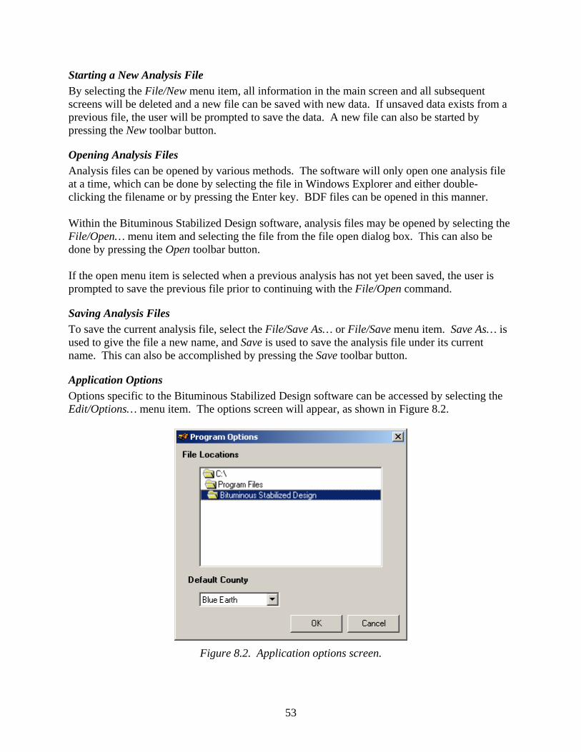
Take the steps... Transportation Research R e s e a r c h...Kn o w l e d g e ...Innov a t i v e Sol u t i o n s ! Design Procedure for Bituminous Stabilized Road Surfaces for Low Volume Roads 2008-28
Transcript
Take the steps...
Transportation Research
Research...Knowledge...Innovative Solutions!
Design Procedure for Bituminous StabilizedRoad Surfaces for Low Volume Roads
2008-28
Technical Report Documentation Page 1. Report No. 2. 3. Recipients Accession No. MN/RC 2008-28 4. Title and Subtitle 5. Report Date
August 2008 6.
Design Procedure for Bituminous Stabilized Road Surfaces for Low Volume Roads
7. Author(s) 8. Performing Organization Report No. Dr. W. James Wilde, P.E. 9. Performing Organization Name and Address 10. Project/Task/Work Unit No.
11. Contract (C) or Grant (G) No.
Minnesota State University, Mankato Center for Transportation Research and Implementation 205 E. Trafton Science Center Mankato, Minnesota 56001
(C) 88193
12. Sponsoring Organization Name and Address 13. Type of Report and Period Covered Final Report 14. Sponsoring Agency Code
Minnesota Department of Transportation 395 John Ireland Boulevard Mail Stop 330 St. Paul, Minnesota 55155 15. Supplementary Notes http://www.lrrb.org/PDF/200828.pdf 16. Abstract (Limit: 200 words)
Many low-volume roadways in the county road system in the State of Minnesota consist of unpaved aggregate surfaces. It is the responsibility of the county engineer to make determinations regarding the design and maintenance of such roads and particularly for specific needs, such as weight restrictions. One method used by several counties in Minnesota is the construction of a bituminous-stabilized layer by adding several inches of new aggregate and stabilizing it with an engineered, water-based asphalt emulsion using mix-in-place methods. This report describes a design method providing highway engineers and their staffs with the technical backing needed for the designs selected.
This report describes the design method for determining the required thickness of stabilized and unstabilized layers in this type of aggregate-surfaced road. This basic design method is based on the material properties and a correlation between layered-elastic analysis, dynamic cone penetrometer, and falling-weight deflectometer testing. The load rating analysis uses the Minnesota Department of Transportation methodology of estimating load rating on low-volume roads using falling weight deflectometer data. A software package is also presented which was developed as part of this project.
No restrictions. Document available from: National Technical Information Services, Springfield, Virginia 22161
19. Security Class (this report) 20. Security Class (this page) 21. No. of Pages 22. Price Unclassified Unclassified 70
Design Procedure for Bituminous Stabilized Road Surfaces for Low Volume Roads
Final Report
Prepared by:
Dr. W. James Wilde, P.E.
Center for Transportation Research and Implementation Minnesota State University, Mankato
August 2008
Published by:
Minnesota Department of Transportation Research Services Section
395 John Ireland Boulevard, MS 330 St. Paul, Minnesota 55155-1899
This report represents the results of research conducted by the authors and does not necessarily represent the views or policies of the Minnesota Department of Transportation. This report does not contain a standard or specified technique. The authors and the Minnesota Department of Transportation do not endorse products or manufacturers. Trade or manufacturers’ names appear herein solely because they are considered essential to this report.
ACKNOWLEDGEMENTS The project team would like to thank the Minnesota Local Road Research Board for its support in funding this project, and the county engineers, Mn/DOT researchers and personnel, and industry representatives who contributed to the project by providing information, suggestions, current practices, and who helped in many other ways toward the success of this project. We also express our gratitude to the members of the technical advisory panel who were instrumental in the development of the project and the associated guidelines. The expertise and experience of the panel members (listed below) were invaluable to the project team throughout the project.
Al Forsberg, Blue Earth County Bob Egan, Dakota County Bill Malin, Chisago County Dennis Luebbe, Rice County Tom Johnson, Midstate Companies Roger Olson, Mn/DOT Office of Materials Dan Wegman, Flint Hills Resources Tom Wood, Mn/DOT Office of Materials
TABLE OF CONTENTS CHAPTER 1. INTRODUCTION ..............................................................................................................1
Background...............................................................................................................................1 CHAPTER 2. LITERATURE REVIEW.....................................................................................................3
Introduction...............................................................................................................................3 Low-Volume Road Design, Materials and Testing ..................................................................3 Economics.................................................................................................................................6 Maintenance..............................................................................................................................6
CHAPTER 3. FIELD STUDIES...............................................................................................................8 Identification and Selection of Field Test Sites ........................................................................8 Field Site Construction .............................................................................................................9 Field Testing .............................................................................................................................9
CHAPTER 4. LABORATORY TESTING................................................................................................17 Summary of Laboratory Tests Conducted..............................................................................17
CHAPTER 5. DESIGN PROCEDURE DEVELOPMENT ...........................................................................22 Data Used in Design Method..................................................................................................23 Required Field Data Collection ..............................................................................................23 Data Analysis..........................................................................................................................25 Layered Elastic Analysis ........................................................................................................28 Load Rating Analysis .............................................................................................................29 Discrete Coefficients ..............................................................................................................30 Linearization of Discrete TONN Adjustment Factors............................................................31
CHAPTER 6. SOFTWARE DEVELOPMENT ..........................................................................................36 Introduction.............................................................................................................................36 Conclusion ..............................................................................................................................41
CHAPTER 7. CHARACTERISTICS AND ECONOMICS OF BITUMINOUS STABILIZED ROADWAYS ..........43 Construction, Maintenance and Rehabilitation.......................................................................43 Benefits of Bituminous Stabilization......................................................................................44 Potential Disadvantages to Bituminous Stabilization.............................................................45 Characteristics of Candidate Projects .....................................................................................46 Economics...............................................................................................................................47
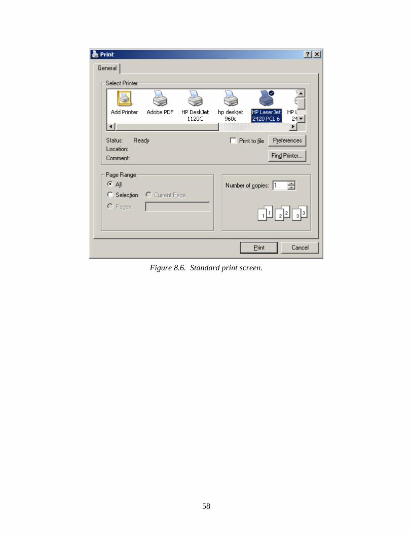
CHAPTER 8. SOFTWARE USER’S MANUAL.......................................................................................51 Bituminous Stabilized Design for Gravel Roads....................................................................51 Introduction.............................................................................................................................51 System Requirements .............................................................................................................51 Installation ..............................................................................................................................51 General Operation...................................................................................................................52 Conducting An Analysis.........................................................................................................54 Printing Results.......................................................................................................................57
CHAPTER 9. CONCLUSIONS AND RECOMMENDATIONS ....................................................................59 Review of Design Procedure ..................................................................................................59 Conclusions.............................................................................................................................59 Recommendations for Additional Research ...........................................................................60 Recommendations for Implementation...................................................................................60
LIST OF TABLES Table 3.1. Basic characteristics of CR 172 and CR 118 sites in Blue Earth County..................... 8 Table 3.2. Layer materials and thicknesses at CR 118 and CR 172. ........................................... 11 Table 5.1. Sample of DCP input data – Blue Earth County Road 48. ......................................... 24 Table 5.2. Sample DCP data adjusted for initial reading............................................................. 26 Table 5.3. Number of blows required to reach specified penetration depth. ............................... 26 Table 5.4. Average and standard deviation of DCP index for each layer.................................... 27 Table 5.5. Reliability and associated standard normal deviates. ................................................. 27 Table 5.6. Deflection ratios for plastic embankments. ................................................................ 32 Table 5.7. Deflection ratios for semi-plastic embankments. ....................................................... 32 Table 5.8. Deflection ratios for non-plastic embankments. ......................................................... 32 Table 5.9. Allowable spring deflections. ..................................................................................... 35
LIST OF FIGURES Figure 3.1. Test sites at CR 172..................................................................................................... 9 Figure 3.2. Test sites at CR 118..................................................................................................... 9 Figure 3.3. Elastic modulus backcalculated from FWD data, August 2005 – CR 118. .............. 11 Figure 3.4. Elastic modulus backcalculated from FWD data, April 2006 – CR 118................... 12 Figure 3.5. Elastic modulus backcalculated from FWD data, August 2005 – CR 172. .............. 13 Figure 3.6. Elastic modulus backcalculated from FWD data, April 2006 – CR 172................... 13 Figure 3.7. DCP results for CR 118, Site 1 – stabilized layer (Top 13 cm). ............................... 14 Figure 3.8. DCP results for CR 118, Site 1 – into subgrade (Top 40 cm). .................................. 15 Figure 3.9. DCP mm/blow vs. rainfall – Site 1, CR 118. ............................................................ 16 Figure 4.1. Emulsion sample in triaxial cell. ............................................................................... 18 Figure 4.2. Resilient modulus results on Class 5 material from CR 172..................................... 19 Figure 4.3. Resilient modulus results on Class 5 material from CR 118..................................... 20 Figure 4.4. Gradation of aggregate obtained from CR 172 and CR 118 projects........................ 21 Figure 5.1. Penetration of DCP hammer on sample sites. ........................................................... 24 Figure 5.2. DCP results – mm/blow vs. depth. ............................................................................ 25 Figure 5.3. DCP index – resilient modulus models. .................................................................... 28 Figure 5.4. Simulated FWD deflection at load plate. .................................................................. 29 Figure 5.5. Sample load rating output.......................................................................................... 31 Figure 5.6. Deflection ratio vs. day of year for plastic embankments. ........................................ 33 Figure 5.7. Deflection ratio vs. day of year for semi-plastic embankments. ............................... 33 Figure 5.8. Deflection ratio vs. day of year for non-plastic embankments.................................. 34 Figure 6.1. Main data entry screen for bituminous stabilized design software. .......................... 36 Figure 6.2. DCP data entry form.................................................................................................. 38 Figure 6.3. FWD data entry form................................................................................................. 39 Figure 6.4. Results of load rating analysis................................................................................... 40 Figure 6.5. Sample printed output from Bituminous Stabilized Design Software. ..................... 41 Figure 7.1. Costs per mile for various maintenance / upgrade options........................................ 49 Figure 7.2. Average annual maintenance and rehabilitation costs per mile. ............................... 50 Figure 8.1. Main bituminous stabilized design screen................................................................. 52 Figure 8.2. Application options screen. ....................................................................................... 53 Figure 8.3. DCP data entry screen. .............................................................................................. 55 Figure 8.4. FWD data entry screen. ............................................................................................. 56 Figure 8.5. Load rating analysis screen. ...................................................................................... 57 Figure 8.6. Standard print screen. ................................................................................................ 58
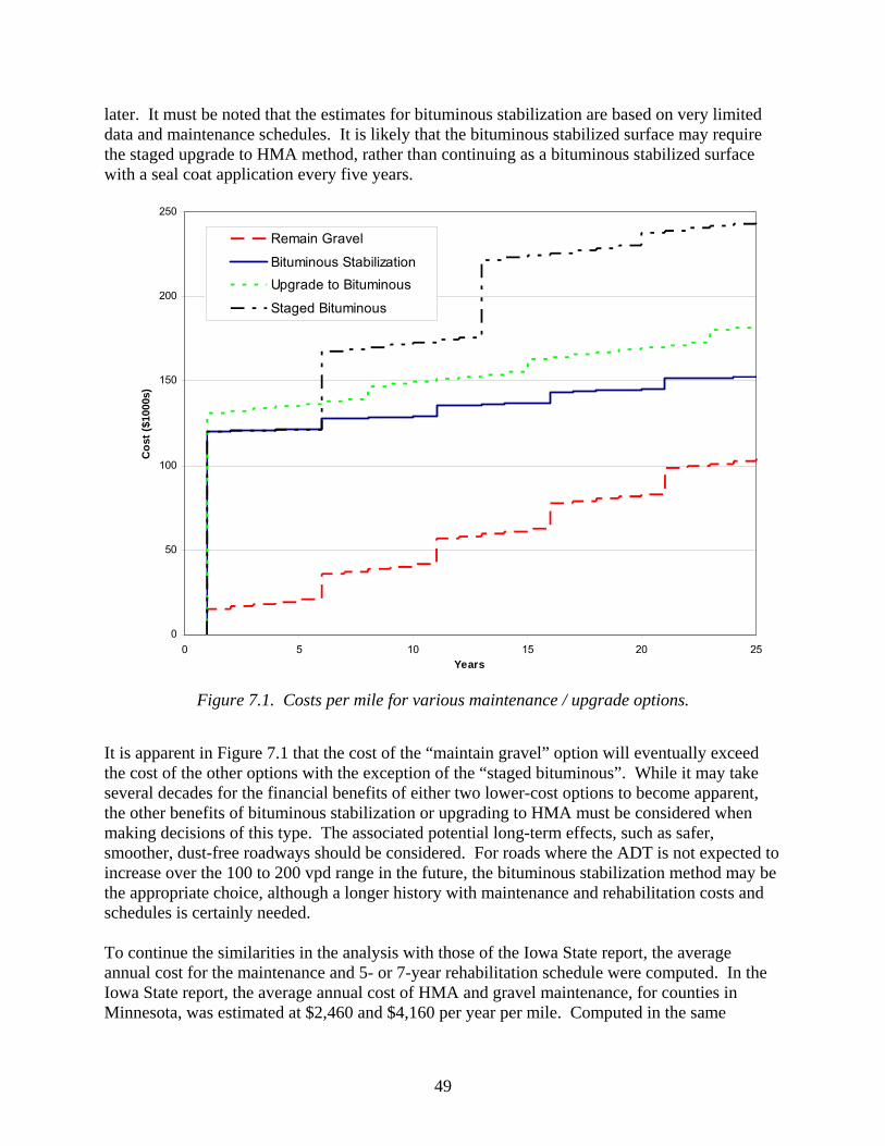
EXECUTIVE SUMMARY This report describes the development of a simple design method for determining the appropriate depth of bituminous stabilization of gravel roads. The process of bituminous stabilization normally includes the placement of several inches of new gravel, followed by stabilization using a full-depth reclaimer, mixing an asphalt emulsion at a specified rate and recompacting the material. One or two seal coats follow the stabilization activities during the first year, and at regular intervals thereafter. This report discusses the materials testing, both in the field and in the laboratory, the analytical methods for determining the strength and predicted deflections in the stabilized roadway, and the application of the existing analysis method for determining the allowable load rating for such a roadway. In addition, this report describes the small software package developed as part of this project, which automates the development of an appropriate thickness of new gravel as well as the depth of stabilization. It also includes a user’s manual for the installation and use of the software. The report also discusses reasonable expectations for this type of roadway, including the benefits that can be expected, and the potential disadvantages and costs that may be involved. It also provides an estimate of the life-cycle costs of this type of construction compared to upgrading a roadway to a bituminous surface and leaving the gravel surface intact. The report ends with recommendations for implementation of the design method and accompanying software. Some of the recommendations include further evaluation of the method for the appropriateness of the thicknesses and depths suggested by the software, and longer periods of time for evaluating the maintenance and rehabilitation needs and associated costs. The process of bituminous stabilization with asphalt emulsion can be beneficial to county and municipal highway agencies in reducing the cost of regraveling and regrading, eliminating the problem of dust, and providing a smoother surface for driving. This type of surface must be well-maintained, however, for if the seal coats which protect the surface and hold the stabilized layer together are damaged, a more expensive rehabilitation may be required.
1
CHAPTER 1. INTRODUCTION
Many roadways in the county road system in the State of Minnesota consist of unpaved aggregate surfaces. For example, Blue Earth County maintains approximately 720 miles on the county road system of which about 300 miles are gravel. It is often the duty of the county engineer to make determinations regarding the pavement design of such roads for a specific need, such as for weight restrictions. One method used by several counties in Minnesota is essentially to create a bituminous-stabilized layer of aggregate in the top several inches of an aggregate-surfaced roadway using one of several currently used mix-in-place methods. This report describes a method for providing county engineers and their staffs with a method to determine the most appropriate thickness of new aggregate and the appropriate depth of stabilization to meet a desired load-carrying capacity. The procedure requires parameters such as soil type, strength, and average daily traffic to conduct the analysis. This method of upgrading aggregate-surfaced roads can save money by eliminating the need for regraveling, can increase safety by improving the driving surface, and reduces dust by effectively binding the fine dust particles in the surface layer. This report discusses the benefits and costs of stabilizing a gravel road with asphalt emulsion, and also presents information regarding the selection of candidate roadways for stabilization. In addition, it discusses the potential problems that can be encountered when constructing and maintaining roads that have been stabilized in this manner.
Background The process of stabilizing aggregate surfaced roadways includes the compaction of up to 10 inches of Class 5 base material, followed by the use of a cold in-place recycling machine to mix approximately 5 percent by weight of an asphalt emulsion into the top 4-7 inches of the new base material. After this mixing process, the surface is again compacted. After 1-2 weeks of curing exposure to the air, a seal coat is placed on the surface. A second seal coat is then placed during the next construction season. It is expected that these types of stabilized pavements will need to receive a seal coat approximately every 5-7 years. There are several reasons for upgrading aggregate surfaced roads in this manner, rather than continuing to maintain the roads in the traditional manner or upgrading the roads with a Hot-mix Asphalt (HMA) surface. The benefits of stabilizing the top several inches has the following benefits:
• reduces or eliminates dust • provides smoother driving surface for the public • reduces or eliminates the loss of gravel • provides better traction for vehicles.
By almost eliminating the loss of gravel, the road surface has a reduced need for periodical addition of gravel to replace that lost. The bituminous stabilization process is also much less expensive than reconstruction with HMA pavement surface. Besides the additional cost of
2
upgrading the roadways to an HMA surface, another limitation to doing this is often the geometric conditions of the roads. Low volume, aggregate surfaced roadways are often not designed for higher operating speeds that drivers would expect from an HMA surfaced roadway. The necessary design, construction, and potential right-of-way costs to upgrade unpaved roadways could be prohibitive, and would not be an economical use of county highway funds. This report focuses on the thickness of the stabilized layer and on material properties for design and construction, using existing methods of determining roadway load ratings, and does not focus on the long-term fatigue characteristics of the materials.
3
CHAPTER 2. LITERATURE REVIEW
Introduction There has been some interest recently in improving aggregate-surface roads and also in determining the economic feasibility of doing so. Several reports have been written which discuss various methods for designing aggregate-surfaced, low-volume roads, procedures for improving these roads, materials-related issues, and economic issues related to these roads. This chapter is divided into sections reflecting the various components of the design method, and relating them to work that has been done previously. These sections are:
• Design, Materials and Testing • Economics • Maintenance
Much of the literature is not specifically oriented toward the design and construction of bituminous-stabilized pavements. The literature that is available that addresses bituminous stabilization is oriented toward base layers in pavement structures. The intent of this literature review is to evaluate the appropriateness of the literature for the application desired in this project. Specifically, this project combines existing low-volume road design methods, laboratory and field testing methods, and the Minnesota Department of Transportationt (Mn/DOT) TONN procedure to estimate the load-carrying capacity of aggregate-surfaced roads in Minnesota.
Low-Volume Road Design, Materials and Testing Beaudry, T., Minnesota’s Design Guide for Low Volume Aggregate Surfaced Roads, Report No. MN/RD-92/11, Minnesota Local Road Research Board, St. Paul, MN, 1992. This report was written to provide a design method using soil factors for counties, townships, and small cities to use in aggregate road design. The method does not require in-depth soil testing, although it does encourage the use of additional test methods in addition to the classification of soils. The report also provides some background information on the US Forest Service Aggregate Road Design Guide. The soil factor design method is simply based on tabulated values of soil factor, based on soil classification. Soil factors range from 50, for gravelly soils, to 130 or more for clays. The tabulated values can be found based on any of three classification systems – Mn/DOT, AASHTO (American Association of State Highway and Transportation Officials), or USCS (Unified Soil Classification System). Layer thicknesses are then determined based on the soil factor and two-way traffic in terms of average daily traffic (ADT) and/or heavy commercial average daily traffic (HCADT). Thicknesses of the surface layer and bases of different materials can then be found in a design table. The US Forest Service design method uses somewhat more testing, and requires a California Bearing Ratio (CBR) value or other soil strength parameter (resilient modulus, dynamic cone penetrometer, etc.) to be correlated with CBR.
4
The report also provides information regarding compaction, drainage, frost heave, and lime stabilization. Skok, E., D. Timm, M. Brown, and T. Clyne, Best Practices for the Design and Construction of Low Volume Roads, Report No. MN/RC-2002-17, Minnesota Local Road Research Board, St. Paul, MN, 2002. The Local Road Research Board (LRRB) published another report titled Best Practices for the Design and Construction of Low Volume Roads. This report was developed primarily for low-volume roads with paved surfaces, and presents details of three design procedures, and provides recommendations for future use. The report describes the advantages and disadvantages of the soil factor, R-Value (Granular Equivalent), and resilient modulus (MnPAVE) methods of pavement design. To correlate strength characteristics of soils, the report refers to a table from the MnPAVE manual which provides basic relationships between soil classification, soil factor, R-Value, CBR, Dynamic Cone Penetrometer (DCP), and resilient modulus values. The material properties and traffic inputs required for the design procedures summarized in this report include the following. Soil Factor
• AASHTO soil classification • Predicted ADT and/or HCADT for design period
R-Value
• AASHTO Soil Classification • Cumulative Equivalent Single Axle Loads (ESALs) over design period • Granular equivalent factors for HMA, base materials, and subgrade
MnPAVE
• Resilient modulus of materials • Cumulative ESALs over design period • Climate • Others depending on the level of analysis desired by the user.
For the purposes of the current research study, the soil factor and R-value design methods will be evaluated. For low-volume roads, the level of input required for the MnPAVE analysis is not reasonable. Erickson, H and A. Drescher, The Use of Geosynthetics to Reinforce Low Volume Roads, Report No. MN/RC-2001-15, Minnesota Department of Transportation, St. Paul, MN, 2001. This report examines the possible benefits to the roadway by reinforcing with stiff geosynthetic material placed between the aggregate base layer and the subgrade of low volume roads. Only reinforcement functions were examined. The finite difference program FLAC was used to conduct experiments on various surfaced and unsurfaced roads. This program was used to output the percent normalized deflection reduction found in the reinforced roadway. It was
5
determined that geosynthetics do in fact provide reinforcement as long as the subgrade material is softer than the geosynthetic fabric. It was also determined that reinforcement may also increase the service life of a roadway due to the reduced deflections of the roadway surface. In all, this report shows that the use of stiff geosynthetic material can definitely increase strength and durability in low volume roads. This report and many like it are of general interest, but not related specifically to the type of stabilization investigated in this project. Kruse, C.G. and E.L. Skok, Flexible Pavement Evaluation with the Benkelman Beam, Minnesota Department of Highways, Investigation 603 Summary Report, 1968. The authors of this report state that the purpose of the investigation was to determine the relationship between the Minnesota Quickie plate bearing test and the Benkelman beam test for predicting the allowable spring load, and to determine the relationship of the two test methods to load carrying capacity, pavement structure, and performance of county roads and municipal streets in Minnesota. The summary section of the report states that a mathematical correlation was developed between the Minnesota Quickie plate bearing test and the Benkelman beam test. Although the primary objective of the project was to develop this correlation, it was not possible due to variation in the data. The study did, however, develop a method for determining allowable spring deflection with the Benkelman beam, based on a literature survey and a related field study. The results of this study were used in the current research when determining the appropriate thickness of asphalt stabilized surface for the load rating desired by the pavement engineer. Forsberg, A.T., Blue Earth County Finn/Oil Gravel Project, Minnesota Department of Transportation, Report No. MN/RC-97/12, April 1997. Blue Earth County constructed an economical stabilized gravel construction project which was reported to cost about 33 percent less than a traditional 7-ton bituminous pavement. After placing seven inches of Class 5 material on the roadway, an additional 2.5 inches of either 100 percent quartzite or 50 percent quartzite / 50 percent gravel were placed, mixed with 4.1 percent and 5 percent asphalt emulsion, on two test sections, respectively. These were mixed in a traditional hot-mix asphalt plant at lower temperatures. While this project did not include a mix-in-place recycling machine, it represents an attempt to find a better way of upgrading aggregate surfaced roadways in a more economical manner. The study found that segregation was a problem with the mix, but attributed it to a coarse aggregate gradation and low asphalt content. The mix also rutted soon after construction and for several weeks after construction, due to the slow curing asphalt emulsion. This was repaired by using the blow-patch method and seal coating. The rutting was rolled flat and has since become stable. The project has since been overlaid, and is providing good service.
6
Bushman, W., T. Freeman, and E. Hoppe, Stabilization Techniques for Unpaved Roads, Report No. VTRC 04-R18, Virginia Transportation Research Council, Charlottesville, VA, 2004. This report examines the effectiveness of soil stabilization products used in unpaved roadways. The application and testing of seven different stabilizing products took place on an unpaved road in Loudon County, Virginia. The study looked at the effects of calcium chloride, magnesium chloride, a soy/lecithin-based product, and three commercial acrylic-based products. Each of the products was deep-mixed into the top few inches of the gravel road with the use of a full-depth reclamation (FDR) machine. The performance of the gravel road stabilized with the various products was measured solely by longitudinal profile once just prior to construction and again several months after construction.
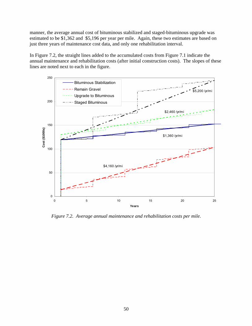
Economics Jahren, C. T., D. Smith, J. Thorius, M. Rukashaza-Mukome, and D. White, Economics of Upgrading an Aggregate Road, Report No. MN/RCD – 2005-09, Iowa State University, Ames, IA, 2005. This report was written to provide Minnesota Counties and townships with information to help them make decisions on when it may be economical to upgrade and pave aggregate roadways. The report compares the cost of maintaining a gravel road against that cost of upgrading to a paved surface. The investigation focused on Waseca and Olmsted Counties and other locations throughout Minnesota. Data from 1997 to 2001 were analyzed to evaluate the maintenance costs of aggregate roads in each county. This information was then compared to an estimated cost of repaving these roads with bituminous material. The study reported several results, including:
• Traffic volumes on gravel roads in Minnesota are increasing steadily. Due to this increase, city, county and township officials are being encouraged to upgrade gravel roads. When traffic volumes increase, so do maintenance costs
• Historical costs may underestimate gravel road maintenance, especially for roads with high traffic volumes.
• Maintenance savings alone could not justify an upgrade, however an upgrade could be justified by other means that cannot easily be assigned monetary values.
The final recommendation is that gravel roads with more than 200 vehicles per day be thoroughly considered for upgrade. For volumes less than this, other justification should be found before upgrading the road surface.
Maintenance Lunsford, G. and J. Mahoney, Dust Control on Low Volume Roads: A Review of Techniques and Chemicals Used, Report No. FHWA-LT-01-002, University of Washington, Seattle, WA, 2001. This report serves as a practical dust control guide for earth of gravel surfaced roads. The report examines the use of standard and non-standard dust suppressants. The standard suppressants examined are salts, lignin sulfides, and emulsions. The non-standard suppressants are enzymes, pozzolans, synthetic polymer emulsions, protection techniques, and recycled waste material.
7
The conclusions of these tests indicate that all work to some extent, but some do not offer environmentally safe solutions and some don’t perform as well in adverse climates. Skorseth, K., and A.A. Selim, Gravel Roads Maintenance and Design Manual, South Dakota Local Transportation Assistance Program, Report No. LTAP-02-002, April, 2005. The South Dakota Local Transportation Assistance Program developed a maintenance and design manual for gravel roads. This manual discusses asphalt stabilization only in the context of dust control, as a maintenance issue. For this purpose, only surface application is recommended by the report. This report also contains information on the benefits of stabilization in general, which concur with those identifies in the current research, which include dust control, loss of aggregate, and reduced blading and shaping maintenance activities and the associated reduction in the cost of new material.
8
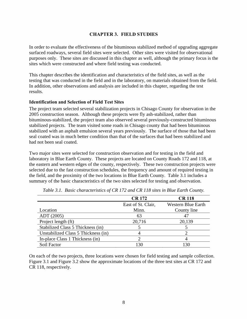
CHAPTER 3. FIELD STUDIES
In order to evaluate the effectiveness of the bituminous stabilized method of upgrading aggregate surfaced roadways, several field sites were selected. Other sites were visited for observational purposes only. These sites are discussed in this chapter as well, although the primary focus is the sites which were constructed and where field testing was conducted. This chapter describes the identification and characteristics of the field sites, as well as the testing that was conducted in the field and in the laboratory, on materials obtained from the field. In addition, other observations and analysis are included in this chapter, regarding the test results.
Identification and Selection of Field Test Sites The project team selected several stabilization projects in Chisago County for observation in the 2005 construction season. Although these projects were fly ash-stabilized, rather than bituminous-stabilized, the project team also observed several previously-constructed bituminous stabilized projects. The team visited some roads in Chisago county that had been bituminous stabilized with an asphalt emulsion several years previously. The surface of those that had been seal coated was in much better condition than that of the surfaces that had been stabilized and had not been seal coated. Two major sites were selected for construction observation and for testing in the field and laboratory in Blue Earth County. These projects are located on County Roads 172 and 118, at the eastern and western edges of the county, respectively. These two construction projects were selected due to the fast construction schedules, the frequency and amount of required testing in the field, and the proximity of the two locations in Blue Earth County. Table 3.1 includes a summary of the basic characteristics of the two sites selected for testing and observation.
Table 3.1. Basic characteristics of CR 172 and CR 118 sites in Blue Earth County.
CR 172 CR 118
Location East of St. Clair,
Minn. Western Blue Earth
County line ADT (2005) 63 47 Project length (ft) 20,716 20,139 Stabilized Class 5 Thickness (in) 5 5 Unstabilized Class 5 Thickness (in) 4 2 In-place Class 1 Thickness (in) 2 4 Soil Factor 130 130
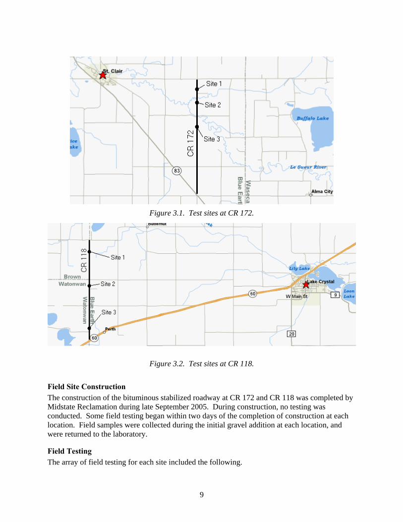
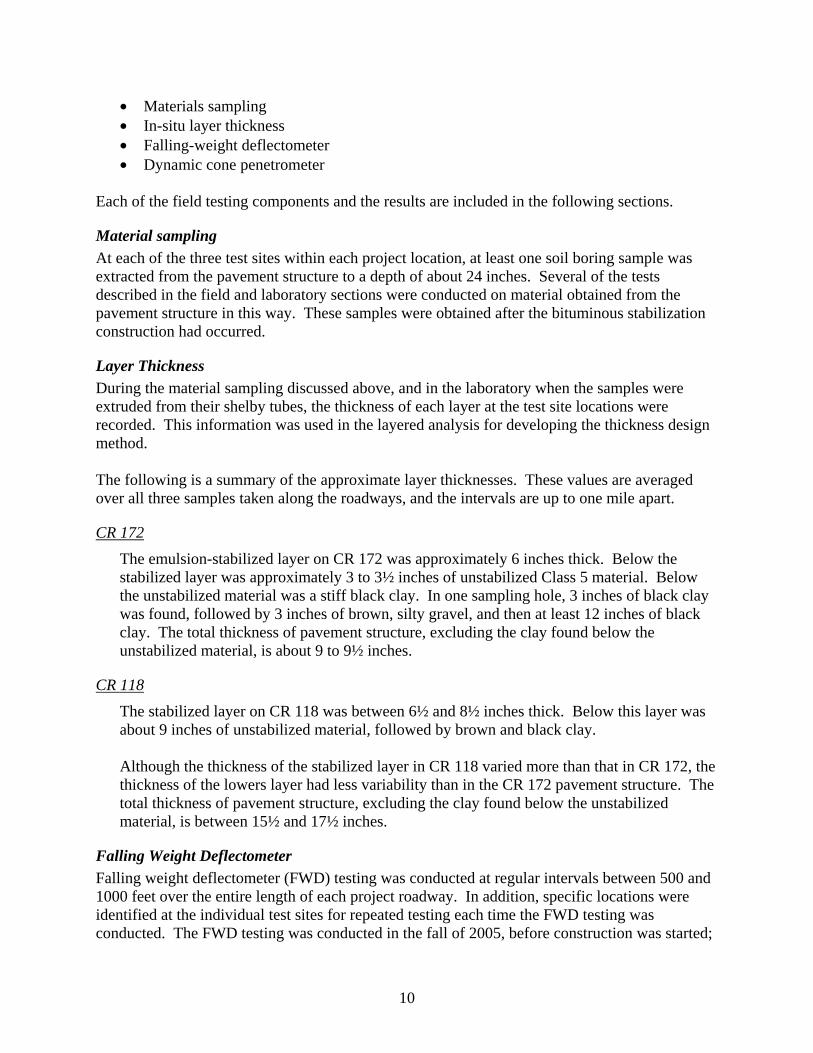
On each of the two projects, three locations were chosen for field testing and sample collection. Figure 3.1 and Figure 3.2 show the approximate locations of the three test sites at CR 172 and CR 118, respectively.
9
Figure 3.1. Test sites at CR 172.
Figure 3.2. Test sites at CR 118.
Field Site Construction The construction of the bituminous stabilized roadway at CR 172 and CR 118 was completed by Midstate Reclamation during late September 2005. During construction, no testing was conducted. Some field testing began within two days of the completion of construction at each location. Field samples were collected during the initial gravel addition at each location, and were returned to the laboratory.
Field Testing The array of field testing for each site included the following.
Each of the field testing components and the results are included in the following sections.
Material sampling At each of the three test sites within each project location, at least one soil boring sample was extracted from the pavement structure to a depth of about 24 inches. Several of the tests described in the field and laboratory sections were conducted on material obtained from the pavement structure in this way. These samples were obtained after the bituminous stabilization construction had occurred.
Layer Thickness During the material sampling discussed above, and in the laboratory when the samples were extruded from their shelby tubes, the thickness of each layer at the test site locations were recorded. This information was used in the layered analysis for developing the thickness design method. The following is a summary of the approximate layer thicknesses. These values are averaged over all three samples taken along the roadways, and the intervals are up to one mile apart.
CR 172
The emulsion-stabilized layer on CR 172 was approximately 6 inches thick. Below the stabilized layer was approximately 3 to 3½ inches of unstabilized Class 5 material. Below the unstabilized material was a stiff black clay. In one sampling hole, 3 inches of black clay was found, followed by 3 inches of brown, silty gravel, and then at least 12 inches of black clay. The total thickness of pavement structure, excluding the clay found below the unstabilized material, is about 9 to 9½ inches.
CR 118
The stabilized layer on CR 118 was between 6½ and 8½ inches thick. Below this layer was about 9 inches of unstabilized material, followed by brown and black clay. Although the thickness of the stabilized layer in CR 118 varied more than that in CR 172, the thickness of the lowers layer had less variability than in the CR 172 pavement structure. The total thickness of pavement structure, excluding the clay found below the unstabilized material, is between 15½ and 17½ inches.
Falling Weight Deflectometer Falling weight deflectometer (FWD) testing was conducted at regular intervals between 500 and 1000 feet over the entire length of each project roadway. In addition, specific locations were identified at the individual test sites for repeated testing each time the FWD testing was conducted. The FWD testing was conducted in the fall of 2005, before construction was started;
11
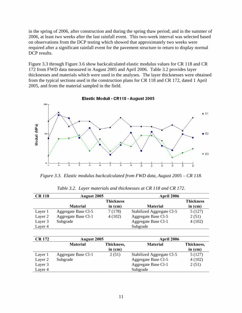
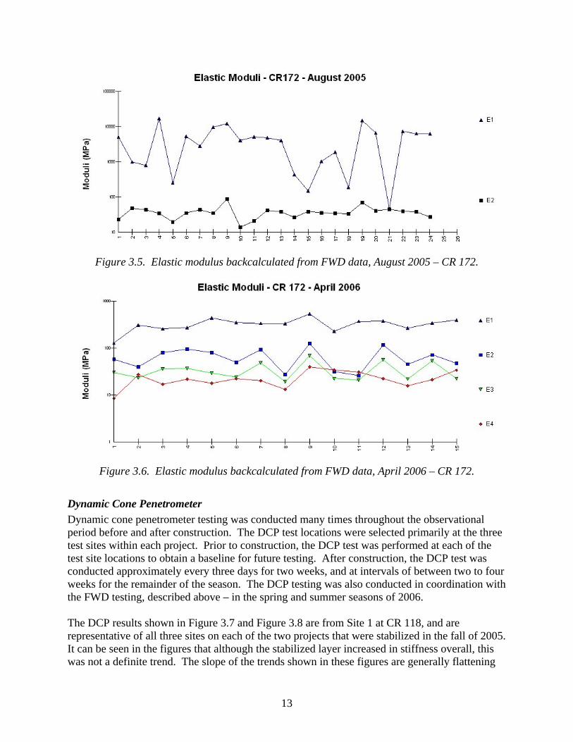
in the spring of 2006, after construction and during the spring thaw period; and in the summer of 2006, at least two weeks after the last rainfall event. This two-week interval was selected based on observations from the DCP testing which showed that approximately two weeks were required after a significant rainfall event for the pavement structure to return to display normal DCP results. Figure 3.3 through Figure 3.6 show backcalculated elastic modulus values for CR 118 and CR 172 from FWD data measured in August 2005 and April 2006. Table 3.2 provides layer thicknesses and materials which were used in the analyses. The layer thicknesses were obtained from the typical sections used in the construction plans for CR 118 and CR 172, dated 1 April 2005, and from the material sampled in the field.
Figure 3.3. Elastic modulus backcalculated from FWD data, August 2005 – CR 118.
Table 3.2. Layer materials and thicknesses at CR 118 and CR 172. CR 118 August 2005 April 2006
Material Thickness
in (cm)
Material Thickness
in (cm) Layer 1 Aggregate Base Cl-5 7 (178) Stabilized Aggregate Cl-5 5 (127) Layer 2 Aggregate Base Cl-1 4 (102) Aggregate Base Cl-5 2 (51) Layer 3 Subgrade Aggregate Base Cl-1 4 (102) Layer 4 Subgrade
CR 172 August 2005 April 2006 Material Thickness,
in (cm) Material Thickness,
in (cm) Layer 1 Aggregate Base Cl-1 2 (51) Stabilized Aggregate Cl-5 5 (127) Layer 2 Subgrade Aggregate Base Cl-5 4 (102) Layer 3 Aggregate Base Cl-1 2 (51) Layer 4 Subgrade
12
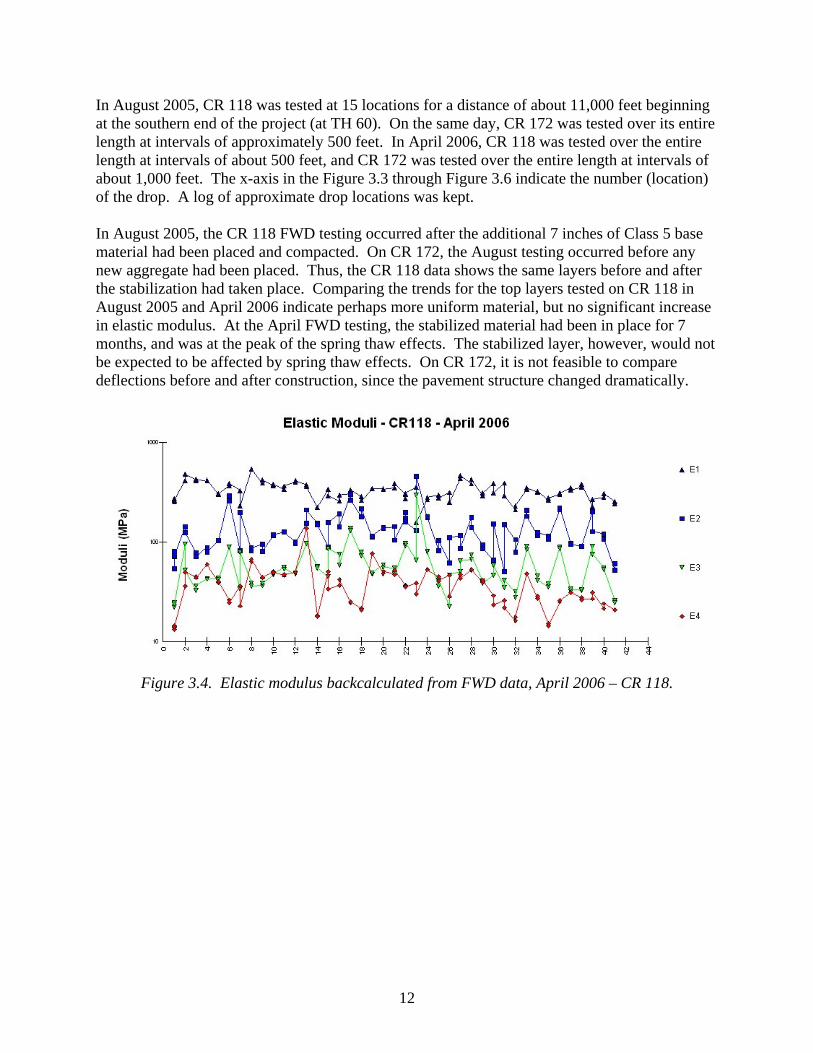
In August 2005, CR 118 was tested at 15 locations for a distance of about 11,000 feet beginning at the southern end of the project (at TH 60). On the same day, CR 172 was tested over its entire length at intervals of approximately 500 feet. In April 2006, CR 118 was tested over the entire length at intervals of about 500 feet, and CR 172 was tested over the entire length at intervals of about 1,000 feet. The x-axis in the Figure 3.3 through Figure 3.6 indicate the number (location) of the drop. A log of approximate drop locations was kept. In August 2005, the CR 118 FWD testing occurred after the additional 7 inches of Class 5 base material had been placed and compacted. On CR 172, the August testing occurred before any new aggregate had been placed. Thus, the CR 118 data shows the same layers before and after the stabilization had taken place. Comparing the trends for the top layers tested on CR 118 in August 2005 and April 2006 indicate perhaps more uniform material, but no significant increase in elastic modulus. At the April FWD testing, the stabilized material had been in place for 7 months, and was at the peak of the spring thaw effects. The stabilized layer, however, would not be expected to be affected by spring thaw effects. On CR 172, it is not feasible to compare deflections before and after construction, since the pavement structure changed dramatically.
Figure 3.4. Elastic modulus backcalculated from FWD data, April 2006 – CR 118.
13
Figure 3.5. Elastic modulus backcalculated from FWD data, August 2005 – CR 172.
Figure 3.6. Elastic modulus backcalculated from FWD data, April 2006 – CR 172.
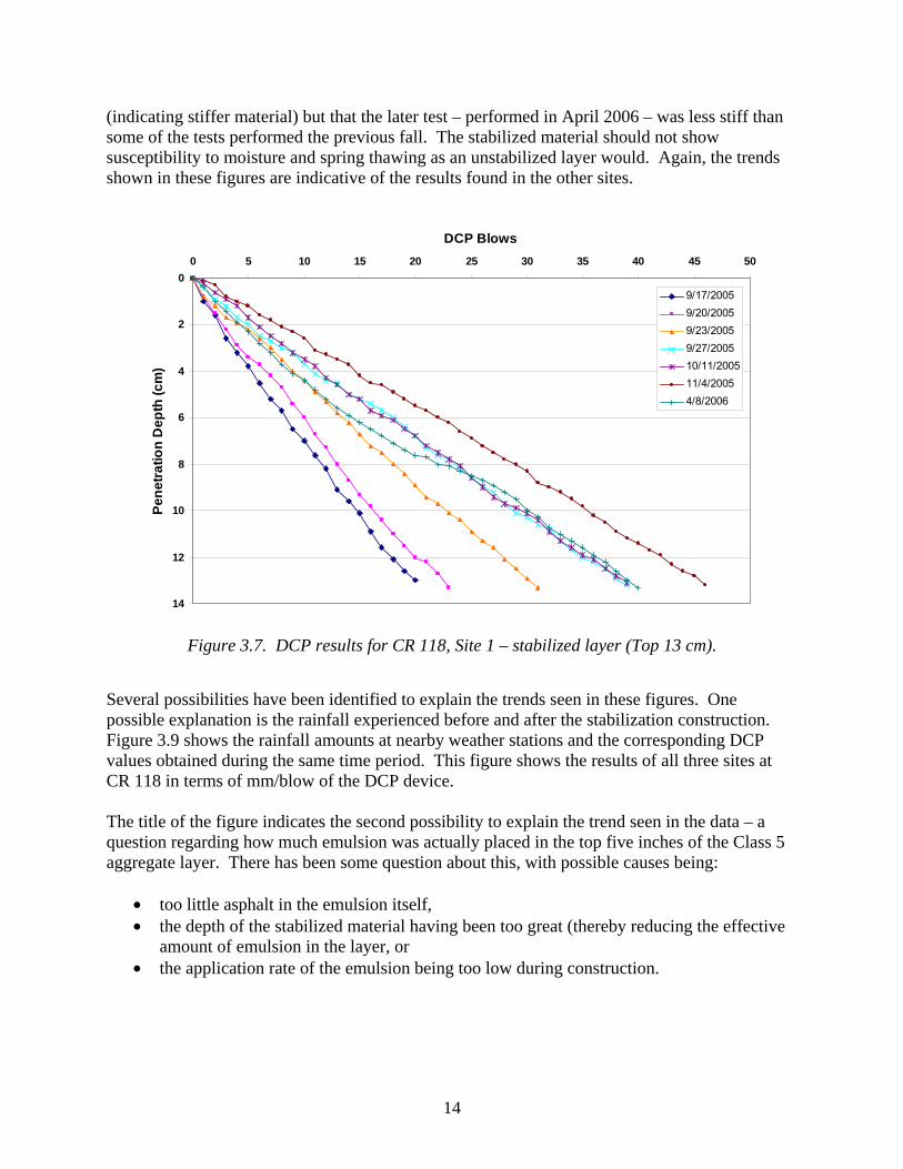
Dynamic Cone Penetrometer Dynamic cone penetrometer testing was conducted many times throughout the observational period before and after construction. The DCP test locations were selected primarily at the three test sites within each project. Prior to construction, the DCP test was performed at each of the test site locations to obtain a baseline for future testing. After construction, the DCP test was conducted approximately every three days for two weeks, and at intervals of between two to four weeks for the remainder of the season. The DCP testing was also conducted in coordination with the FWD testing, described above – in the spring and summer seasons of 2006. The DCP results shown in Figure 3.7 and Figure 3.8 are from Site 1 at CR 118, and are representative of all three sites on each of the two projects that were stabilized in the fall of 2005. It can be seen in the figures that although the stabilized layer increased in stiffness overall, this was not a definite trend. The slope of the trends shown in these figures are generally flattening
14
(indicating stiffer material) but that the later test – performed in April 2006 – was less stiff than some of the tests performed the previous fall. The stabilized material should not show susceptibility to moisture and spring thawing as an unstabilized layer would. Again, the trends shown in these figures are indicative of the results found in the other sites.
Figure 3.7. DCP results for CR 118, Site 1 – stabilized layer (Top 13 cm).
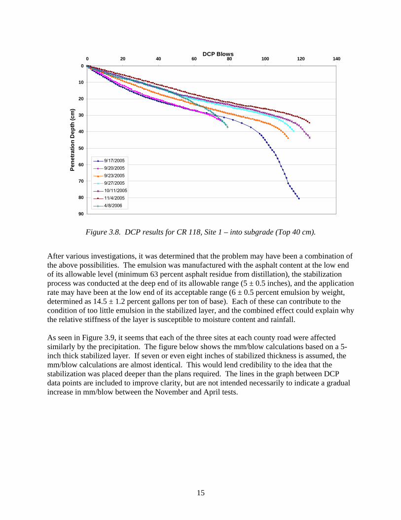
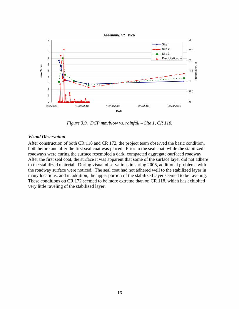
Several possibilities have been identified to explain the trends seen in these figures. One possible explanation is the rainfall experienced before and after the stabilization construction. Figure 3.9 shows the rainfall amounts at nearby weather stations and the corresponding DCP values obtained during the same time period. This figure shows the results of all three sites at CR 118 in terms of mm/blow of the DCP device. The title of the figure indicates the second possibility to explain the trend seen in the data – a question regarding how much emulsion was actually placed in the top five inches of the Class 5 aggregate layer. There has been some question about this, with possible causes being:
• too little asphalt in the emulsion itself, • the depth of the stabilized material having been too great (thereby reducing the effective
amount of emulsion in the layer, or • the application rate of the emulsion being too low during construction.
Figure 3.8. DCP results for CR 118, Site 1 – into subgrade (Top 40 cm).
After various investigations, it was determined that the problem may have been a combination of the above possibilities. The emulsion was manufactured with the asphalt content at the low end of its allowable level (minimum 63 percent asphalt residue from distillation), the stabilization process was conducted at the deep end of its allowable range (5 ± 0.5 inches), and the application rate may have been at the low end of its acceptable range (6 ± 0.5 percent emulsion by weight, determined as 14.5 ± 1.2 percent gallons per ton of base). Each of these can contribute to the condition of too little emulsion in the stabilized layer, and the combined effect could explain why the relative stiffness of the layer is susceptible to moisture content and rainfall. As seen in Figure 3.9, it seems that each of the three sites at each county road were affected similarly by the precipitation. The figure below shows the mm/blow calculations based on a 5-inch thick stabilized layer. If seven or even eight inches of stabilized thickness is assumed, the mm/blow calculations are almost identical. This would lend credibility to the idea that the stabilization was placed deeper than the plans required. The lines in the graph between DCP data points are included to improve clarity, but are not intended necessarily to indicate a gradual increase in mm/blow between the November and April tests.
16
Assuming 5" Thick
0
1
2
3
4
5
6
7
8
9
10
9/5/2005 10/25/2005 12/14/2005 2/2/2006 3/24/2006
Date
mm
/Blo
w
0
0.5
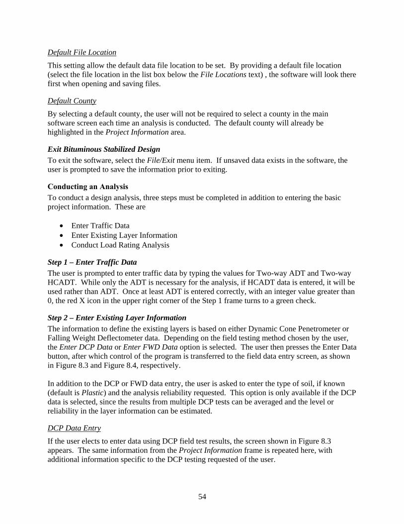
1
1.5
2
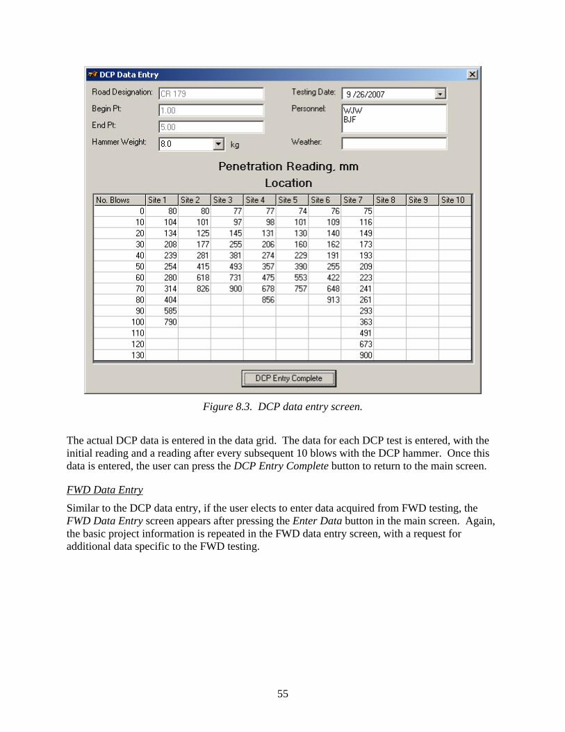
2.5
3
Prec
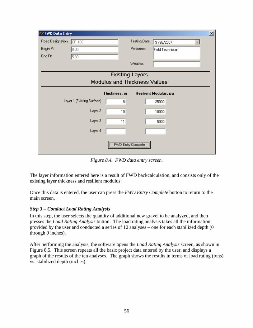
ipita
tion,
in
Site 1Site 2Site 3Precipitation, in
Figure 3.9. DCP mm/blow vs. rainfall – Site 1, CR 118.
Visual Observation After construction of both CR 118 and CR 172, the project team observed the basic condition, both before and after the first seal coat was placed. Prior to the seal coat, while the stabilized roadways were curing the surface resembled a dark, compacted aggregate-surfaced roadway. After the first seal coat, the surface it was apparent that some of the surface layer did not adhere to the stabilized material. During visual observations in spring 2006, additional problems with the roadway surface were noticed. The seal coat had not adhered well to the stabilized layer in many locations, and in addition, the upper portion of the stabilized layer seemed to be raveling. These conditions on CR 172 seemed to be more extreme than on CR 118, which has exhibited very little raveling of the stabilized layer.
17
CHAPTER 4. LABORATORY TESTING
Laboratory testing was conducted to characterize the materials used in the CR 172 and 118 stabilization construction. This chapter describes the testing conducted on each of the materials, and the results obtained.
Summary of Laboratory Tests Conducted This section details the laboratory testing and data analysis conducted on material samples from County Roads 118 and 172 in Blue Earth County, Minnesota. The laboratory testing included the following.
• Soil classification • Gradation • In-situ moisture content • Maximum density and optimum moisture content of Class 5 material • Resilient modulus of stabilized Class 5 material
Samples of unbound aggregates, soils, and the stabilized layer were obtained in the field, as described in the previous chapter on field testing. This chapter discusses the results of the laboratory testing conducted on the samples obtained from the field and emulsion samples obtained from the manufacturer.
Classification Each of the soils sampled were tested for compliance with the Mn/DOT requirements for Class 5 material, based on its gradation. The gravel samples obtained from both sites met the requirements.
In-situ Moisture Content The in-situ moisture content of each soil layer was measured in the laboratory after extrusion from the shelby tubes.
Proctor Density of Class 5 Aggregate Samples of Mn/DOT Class 5 aggregate were obtained during the initial construction phase – placement of seven and nine inches of new gravel on CR 118 and CR 172, respectively. These samples were taken to the laboratory for maximum theoretical density testing.
Resilient Modulus Some of the Class 5 material samples from the gravel operations at the project locations was used in resilient modulus testing in the laboratory. The resilient modulus test was conducted according to AASHTO TP-46, and was used to test unbound materials obtained from the project locations, as well as material that had been stabilized and compacted to the same density as in the field. The resilient modulus testing occurred over several stages. The first stage was to prepare samples using Class 5 material obtained from the field and emulsion obtained from the
18
manufacturer. Samples were prepared using 4x8 inch cylinder molds and compacted to densities ranging from 128 to 138 lbs/cf, with 4 percent moisture content. A total of six samples were compacted for each of County Roads 172 and 118 in Blue Earth County. Two samples were produced at each emulsion content, at 5.5, 6.5, and 7.5 percent. The prepared samples were then allowed to cure, uncovered, for a period of between two and three weeks before testing.
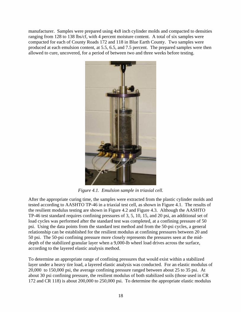
Figure 4.1. Emulsion sample in triaxial cell.
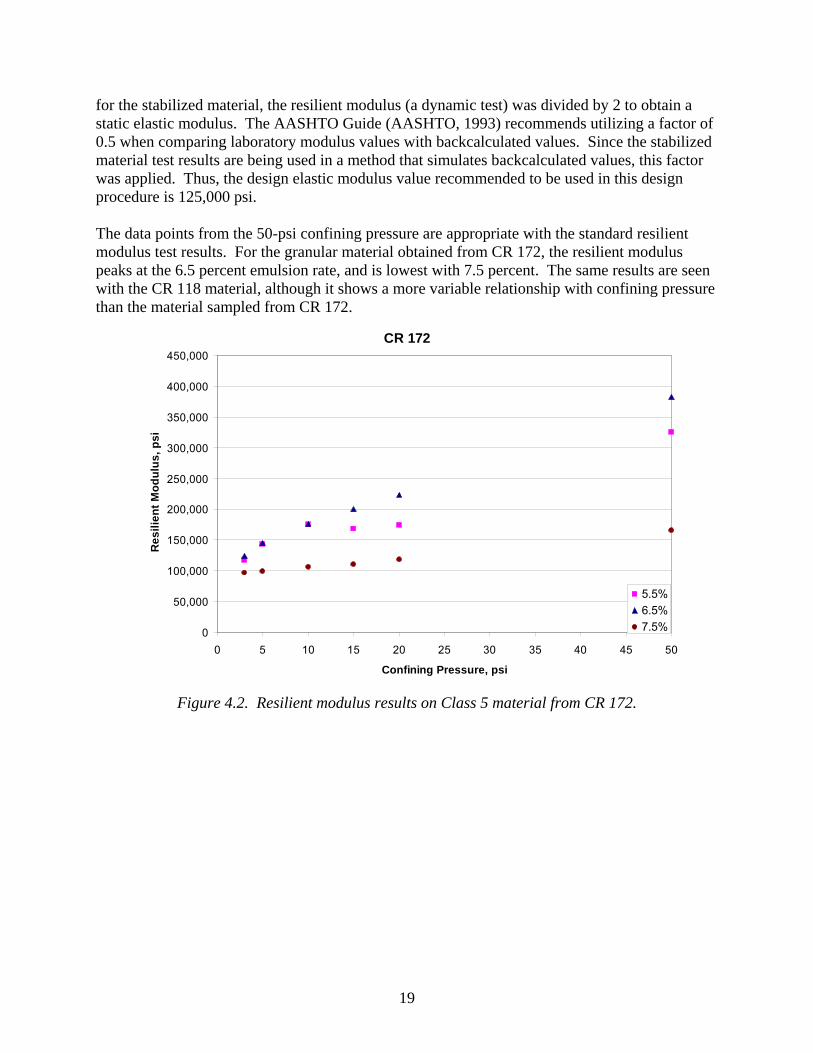
After the appropriate curing time, the samples were extracted from the plastic cylinder molds and tested according to AASHTO TP-46 in a triaxial test cell, as shown in Figure 4.1. The results of the resilient modulus testing are shown in Figure 4.2 and Figure 4.3. Although the AASHTO TP-46 test standard requires confining pressures of 3, 5, 10, 15, and 20 psi, an additional set of load cycles was performed after the standard test was completed, at a confining pressure of 50 psi. Using the data points from the standard test method and from the 50-psi cycles, a general relationship can be established for the resilient modulus at confining pressures between 20 and 50 psi. The 50-psi confining pressure more closely represents the pressures seen at the mid-depth of the stabilized granular layer when a 9,000-lb wheel load drives across the surface, according to the layered elastic analysis method. To determine an appropriate range of confining pressures that would exist within a stabilized layer under a heavy tire load, a layered elastic analysis was conducted. For an elastic modulus of 20,000 to 150,000 psi, the average confining pressure ranged between about 25 to 35 psi. At about 30 psi confining pressure, the resilient modulus of both stabilized soils (those used in CR 172 and CR 118) is about 200,000 to 250,000 psi. To determine the appropriate elastic modulus
19
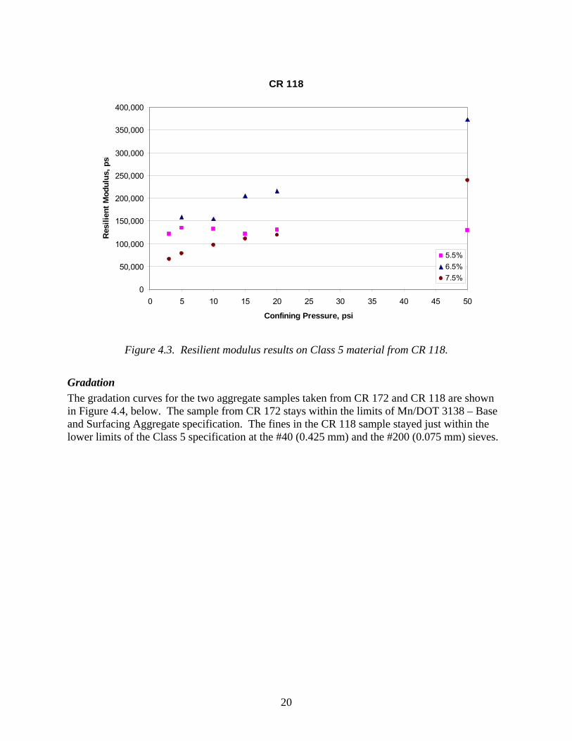
for the stabilized material, the resilient modulus (a dynamic test) was divided by 2 to obtain a static elastic modulus. The AASHTO Guide (AASHTO, 1993) recommends utilizing a factor of 0.5 when comparing laboratory modulus values with backcalculated values. Since the stabilized material test results are being used in a method that simulates backcalculated values, this factor was applied. Thus, the design elastic modulus value recommended to be used in this design procedure is 125,000 psi. The data points from the 50-psi confining pressure are appropriate with the standard resilient modulus test results. For the granular material obtained from CR 172, the resilient modulus peaks at the 6.5 percent emulsion rate, and is lowest with 7.5 percent. The same results are seen with the CR 118 material, although it shows a more variable relationship with confining pressure than the material sampled from CR 172.
CR 172
0
50,000
100,000
150,000
200,000
250,000
300,000
350,000
400,000
450,000
0 5 10 15 20 25 30 35 40 45 50
Confining Pressure, psi
Res
ilien
t Mod
ulus
, psi
5.5%6.5%7.5%
Figure 4.2. Resilient modulus results on Class 5 material from CR 172.
20
CR 118
0
50,000
100,000
150,000
200,000
250,000
300,000
350,000
400,000
0 5 10 15 20 25 30 35 40 45 50
Confining Pressure, psi
Res
ilien
t Mod
ulus
, psi
5.5%6.5%7.5%
Figure 4.3. Resilient modulus results on Class 5 material from CR 118.
Gradation The gradation curves for the two aggregate samples taken from CR 172 and CR 118 are shown in Figure 4.4, below. The sample from CR 172 stays within the limits of Mn/DOT 3138 – Base and Surfacing Aggregate specification. The fines in the CR 118 sample stayed just within the lower limits of the Class 5 specification at the #40 (0.425 mm) and the #200 (0.075 mm) sieves.
21
0
10
20
30
40
50
60
70
80
90
100
0.01 0.1 1 10 100
Sieve Size, mm
Per
cent
Pas
sing
CR 172CR 118Mn/DOT Class 5 Limits
#200
1"
Figure 4.4. Gradation of aggregate obtained from CR 172 and CR 118 projects.
In situ moisture content of the unstabilized material was found to be between 2 and 3 percent. The moisture content in the stabilized material was negligible.
Maximum Density The maximum unit weight on Class 5 aggregate obtained from the CR 118 project, averaged over two tests, was measured at 137.0 pcf. The optimum moisture content at the maximum unit weight was 11.5 percent. The maximum unit weight on CR 172, also averaged over two tests, was measured at 137.6 pcf. The optimum moisture content at the maximum unit weight was 10.8 percent.
22
CHAPTER 5. DESIGN PROCEDURE DEVELOPMENT
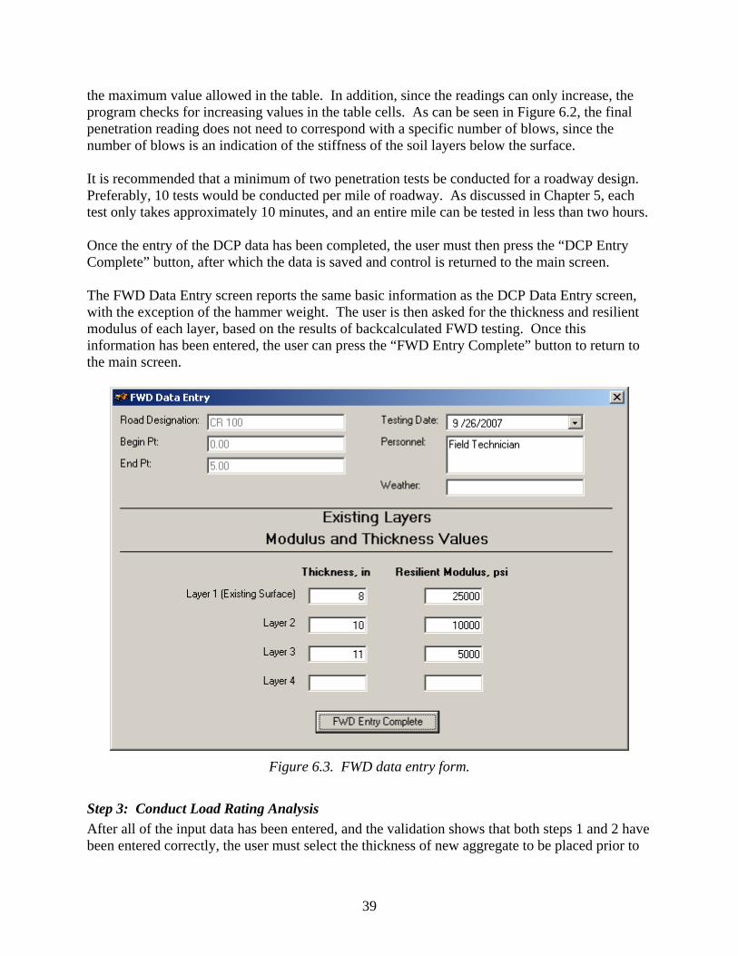
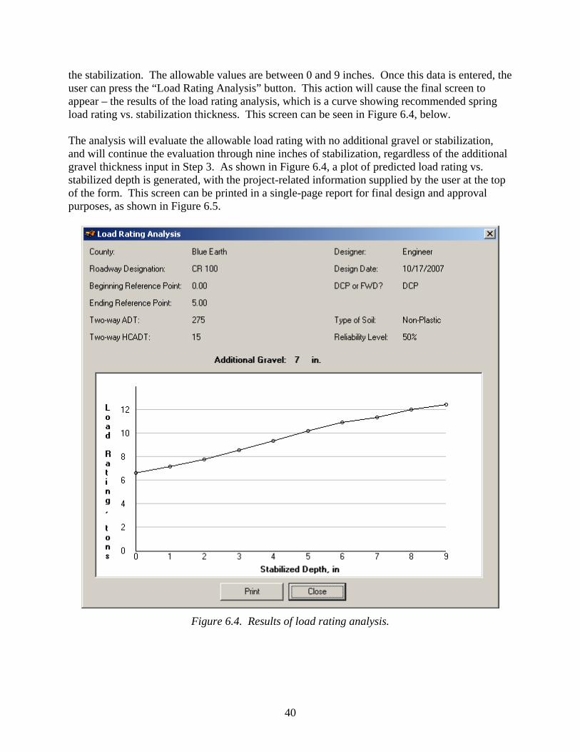
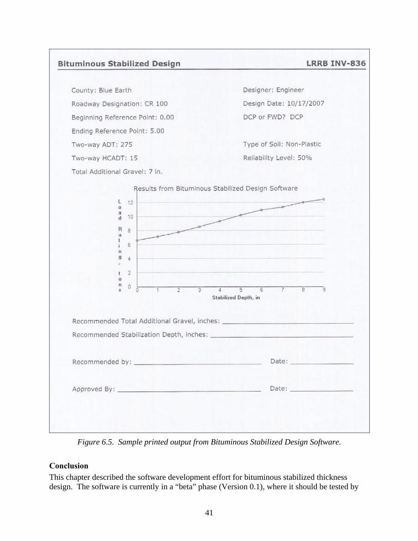
This chapter describes the analysis of field and laboratory data and the development of the design procedure for thickness of bituminous stabilization for low-volume roads. Much of the data has been analyzed in previous chapters. The major focus of this chapter is to combine the information into a cohesive method for determining the appropriate thickness of bituminous-stabilized layer to achieve the desired load rating. The thickness design method described in this report is in draft form, and should be reviewed by practitioners and others involved in gravel road and bituminous design prior to its use for design or construction purposes. This method should be validated using new design and construction projects which were not available for observation and testing during the development of the method. The design procedure is contained in a Microsoft Visual Basic software package, which is a standalone program with an accompanying software installation wizard. This software can be installed on any computer running newer versions of the Microsoft Windows operating system. The software is described in more detail in Chapter 6, and a User’s Guide is provided in Chapter 8. The basic process for the thickness design method described in this report is as follows.
1. Obtain stiffness data for the existing unbound, aggregate-surfaced roadway using either dynamic cone penetrometer or falling-weight deflectometer.
2. If DCP is used, convert DCP index to estimated elastic modulus of layers. If layer thicknesses are not known, these are estimated by the results of the DCP analysis. If FWD is used, estimated elastic modulus of the layers by backcalculation.
3. Select trial values for thickness of additional Mn/DOT Class 5 material and the depth to which the bituminous stabilization will be constructed.
4. Input the estimated layer thicknesses and elastic moduli into a layered-elastic analysis to estimate the surface deflection from FWD testing after the stabilization is complete.
5. Input the estimated surface deflection into the Mn/DOT TONN analysis to determine load rating.
6. If the load rating is not adequate, increase the thickness of stabilized material until a satisfactory rating is estimated.
In the software package, most of the above steps are automated, and a graph of possible designs is produced, thicknesses and stabilization depths from which the pavement design engineer can select depending on the desired spring load rating. One limitation of this design method is that it is dependent on the Mn/DOT TONN analysis, for which some modifications have been made. These limitations and modifications are described at the end of this chapter. The following sections describe the data collected and used in the design method, the steps in the analysis for obtaining the load rating, the field data required of users of the method, and a sensitivity analysis of the method to variations in the inputs.
23
Data Used in Design Method Both field and laboratory data have been used in the development of this design method. Below is a summary of the field and laboratory data that were collected during the project. The results of these tests can be found in previous chapters. Field Data
• Material gradation • Maximum density and optimum moisture content • Resilient modulus of stabilized material
The method described in this chapter uses the DCP index or the FWD backcalculated moduli as inputs, and produces a range of bituminous-stabilized layer thickness with associated, predicted spring load ratings.
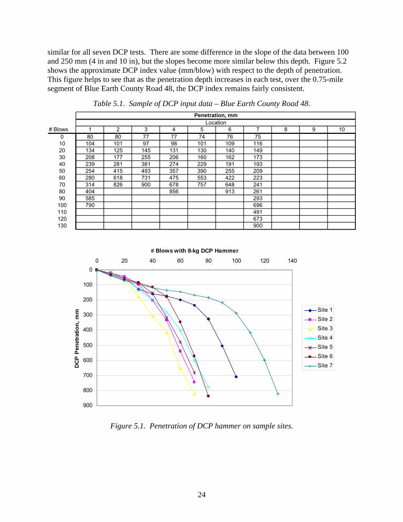
Required Field Data Collection The amount of data collection required by the design method can vary, depending on the amount of coverage desired by the agency using it. The type of data required to conduct the analysis is either DCP or FWD data. To begin the design process, the agency using the design method will collect DCP or FWD data from the aggregate-surfaced roadway in question. As mentioned above, the quantity of data can vary. A minimum of five DCP or FWD sites per mile should be tested in order to provide a statistical basis for the analysis. A minimum of 10 sites per mile is recommended. In an average hour, with very little traffic, about six or seven DCP sites can be tested. Thus, for 10 sites per mile, approximately 100 minutes per mile will be required. FWD data, after the initial setup procedures, can be collected more quickly than DCP data. Table 5.1 shows a sample of the data required for the DCP input method. This set of data was collected at approximately 0.1-mile intervals on Blue Earth County Road 48, near Madison Lake, Minnesota. This is a roadway which has not been stabilized, but which could be a good candidate for such improvements. The data used for this design method should be collected according to the most current revision of American Society for Testing and Materials (ASTM) D6951 (currently 2003) Standard Test Method for Use of the Dynamic Cone Penetrometer in Shallow Pavement Applications. The standard does not specify the number of blows between readings, however to make the data collection occur more quickly and with less complexity, this thickness design method requires one reading of the DCP scale for every 10 blows with the DCP hammer. Figure 5.1 shows a plot vs. depth of the penetration values recorded in the table below. In this figure, the data have been corrected for the initial reading, so that the penetration at zero blows is zero. It can be seen that the slope of the penetration data, for the top 100 mm (4 in) is very
24
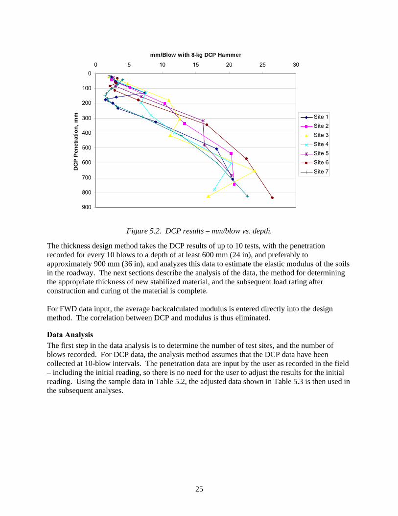
similar for all seven DCP tests. There are some difference in the slope of the data between 100 and 250 mm (4 in and 10 in), but the slopes become more similar below this depth. Figure 5.2 shows the approximate DCP index value (mm/blow) with respect to the depth of penetration. This figure helps to see that as the penetration depth increases in each test, over the 0.75-mile segment of Blue Earth County Road 48, the DCP index remains fairly consistent.
Table 5.1. Sample of DCP input data – Blue Earth County Road 48.
Figure 5.1. Penetration of DCP hammer on sample sites.
25
0
100
200
300
400
500
600
700
800
900
0 5 10 15 20 25 30
mm/Blow with 8-kg DCP Hammer
DCP
Pene
tratio
n, m
m Site 1Site 2Site 3Site 4Site 5Site 6Site 7
Figure 5.2. DCP results – mm/blow vs. depth.
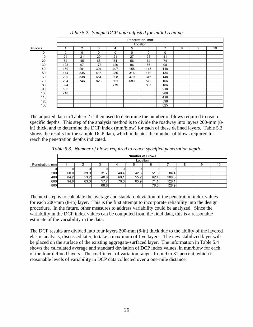
The thickness design method takes the DCP results of up to 10 tests, with the penetration recorded for every 10 blows to a depth of at least 600 mm (24 in), and preferably to approximately 900 mm (36 in), and analyzes this data to estimate the elastic modulus of the soils in the roadway. The next sections describe the analysis of the data, the method for determining the appropriate thickness of new stabilized material, and the subsequent load rating after construction and curing of the material is complete. For FWD data input, the average backcalculated modulus is entered directly into the design method. The correlation between DCP and modulus is thus eliminated.
Data Analysis The first step in the data analysis is to determine the number of test sites, and the number of blows recorded. For DCP data, the analysis method assumes that the DCP data have been collected at 10-blow intervals. The penetration data are input by the user as recorded in the field – including the initial reading, so there is no need for the user to adjust the results for the initial reading. Using the sample data in Table 5.2, the adjusted data shown in Table 5.3 is then used in the subsequent analyses.
26
Table 5.2. Sample DCP data adjusted for initial reading.
The adjusted data in Table 5.2 is then used to determine the number of blows required to reach specific depths. This step of the analysis method is to divide the roadway into layers 200-mm (8-in) thick, and to determine the DCP index (mm/blow) for each of these defined layers. Table 5.3 shows the results for the sample DCP data, which indicates the number of blows required to reach the penetration depths indicated.
Table 5.3. Number of blows required to reach specified penetration depth.
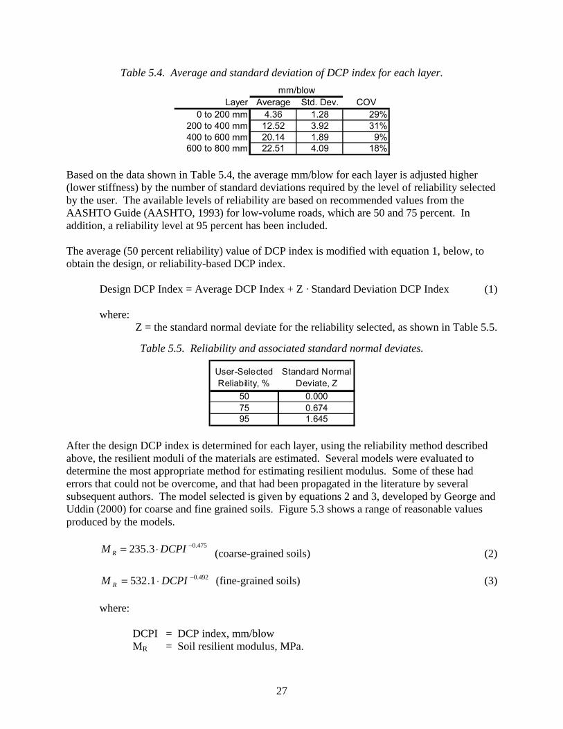
The next step is to calculate the average and standard deviation of the penetration index values for each 200-mm (8-in) layer. This is the first attempt to incorporate reliability into the design procedure. In the future, other measures to address variability could be analyzed. Since the variability in the DCP index values can be computed from the field data, this is a reasonable estimate of the variability in the data. The DCP results are divided into four layers 200-mm (8-in) thick due to the ability of the layered elastic analysis, discussed later, to take a maximum of five layers. The new stabilized layer will be placed on the surface of the existing aggregate-surfaced layer. The information in Table 5.4 shows the calculated average and standard deviation of DCP index values, in mm/blow for each of the four defined layers. The coefficient of variation ranges from 9 to 31 percent, which is reasonable levels of variability in DCP data collected over a one-mile distance.
27
Table 5.4. Average and standard deviation of DCP index for each layer.
Layer Average Std. Dev. COV0 to 200 mm 4.36 1.28 29%
200 to 400 mm 12.52 3.92 31%400 to 600 mm 20.14 1.89 9%600 to 800 mm 22.51 4.09 18%
mm/blow
Based on the data shown in Table 5.4, the average mm/blow for each layer is adjusted higher (lower stiffness) by the number of standard deviations required by the level of reliability selected by the user. The available levels of reliability are based on recommended values from the AASHTO Guide (AASHTO, 1993) for low-volume roads, which are 50 and 75 percent. In addition, a reliability level at 95 percent has been included. The average (50 percent reliability) value of DCP index is modified with equation 1, below, to obtain the design, or reliability-based DCP index. Design DCP Index = Average DCP Index + Z · Standard Deviation DCP Index (1) where: Z = the standard normal deviate for the reliability selected, as shown in Table 5.5.
Table 5.5. Reliability and associated standard normal deviates.
User-Selected Reliability, %
Standard Normal Deviate, Z
50 0.00075 0.67495 1.645
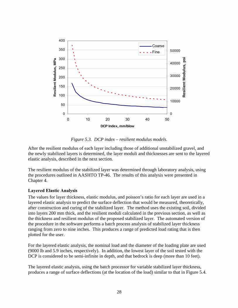
After the design DCP index is determined for each layer, using the reliability method described above, the resilient moduli of the materials are estimated. Several models were evaluated to determine the most appropriate method for estimating resilient modulus. Some of these had errors that could not be overcome, and that had been propagated in the literature by several subsequent authors. The model selected is given by equations 2 and 3, developed by George and Uddin (2000) for coarse and fine grained soils. Figure 5.3 shows a range of reasonable values produced by the models.
After the resilient modulus of each layer including those of additional unstabilized gravel, and the newly stabilized layers is determined, the layer moduli and thicknesses are sent to the layered elastic analysis, described in the next section. The resilient modulus of the stabilized layer was determined through laboratory analysis, using the procedures outlined in AASHTO TP-46. The results of this analysis were presented in Chapter 4.
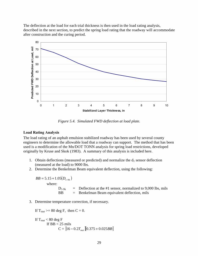
Layered Elastic Analysis The values for layer thickness, elastic modulus, and poisson’s ratio for each layer are used in a layered elastic analysis to predict the surface deflection that would be measured, theoretically, after construction and curing of the stabilized layer. The method uses the existing soil, divided into layers 200 mm thick, and the resilient moduli calculated in the previous section, as well as the thickness and resilient modulus of the proposed stabilized layer. The automated version of the procedure in the software performs a batch process analysis of stabilized layer thickness ranging from zero to nine inches. This produces a range of predicted load rating that is then plotted for the user. For the layered elastic analysis, the nominal load and the diameter of the loading plate are used (9000 lb and 5.9 inches, respectively). In addition, the lowest layer of the soil tested with the DCP is considered to be semi-infinite in depth, and that bedrock is deep (more than 10 feet). The layered elastic analysis, using the batch processor for variable stabilized layer thickness, produces a range of surface deflections (at the location of the load) similar to that in Figure 5.4.
29
The deflection at the load for each trial thickness is then used in the load rating analysis, described in the next section, to predict the spring load rating that the roadway will accommodate after construction and the curing period.
0
10
20
30
40
50
60
70
80
0 1 2 3 4 5 6 7 8 9 10
Stabilized Layer Thickness, in
Pred
icte
d FW
D D
efle
ctio
n at
Loa
d, m
il
Figure 5.4. Simulated FWD deflection at load plate.
Load Rating Analysis The load rating of an asphalt emulsion stabilized roadway has been used by several county engineers to determine the allowable load that a roadway can support. The method that has been used is a modification of the Mn/DOT TONN analysis for spring load restrictions, developed originally by Kruse and Skok (1983). A summary of this analysis is included here.
1. Obtain deflections (measured or predicted) and normalize the d1 sensor deflection (measured at the load) to 9000 lbs.
2. Determine the Benkelman Beam equivalent deflection, using the following: ( )kDBB 9105.115.5 −+= where: D1-9k = Deflection at the #1 sensor, normalized to 9,000 lbs, mils BB = Benkelman Beam equivalent deflection, mils
3. Determine temperature correction, if necessary. If Tmat >= 80 deg F, then C = 0. If Tmat < 80 deg F If BB < 25 mils C = [ ][ ]BBTmat 025.0375.02.016 +−
30
If 25 <= BB <=35 mils C = [ ]matT2.016 − If BB > 35 mils C = [ ][ ]BBTmat 025.0125.02.016 +− where: Tmat = temperature of the stabilized mat, deg F. C = correction factor.
4. Determine BB deflection at 80 deg F.
CBBBB +=80 5. Convert BB80 to spring deflection.
( )rS dBBBB 80= where: BB80 = equivalent Benkelman Beam deflection at 80 deg. F, mils BBS = equivalent deflection during spring thaw, mils dr = deflection ratio: spring deflections compared to deflections at other
non-frozen times of the year. This value is obtained from tables in the Kruse and Skok (1983) report.
6. Determine the Allowable Deflection (AD), which is simply 90 percent of the Allowable
Spring Deflection. The allowable spring deflection is also found in a table in the referenced reports.
7. Determine Allowable Axle Load (LA), in tons, as follows:
⎟⎟⎠
⎞⎜⎜⎝
⎛=
SA BB
ADL 10
Using the load rating analysis summarized above, predicted FWD deflections using DCP or FWD data can be used to determine the allowable load rating. Actual FWD measurements must be backcalculated to determine the elastic modulus of the existing layers. The simulation will then analyze the existing structure with an addition of new gravel and stabilized material at various thicknesses.
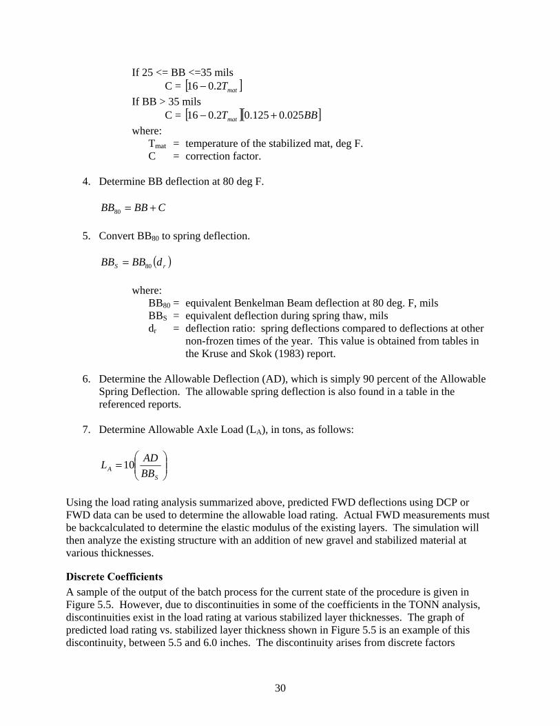
Discrete Coefficients A sample of the output of the batch process for the current state of the procedure is given in Figure 5.5. However, due to discontinuities in some of the coefficients in the TONN analysis, discontinuities exist in the load rating at various stabilized layer thicknesses. The graph of predicted load rating vs. stabilized layer thickness shown in Figure 5.5 is an example of this discontinuity, between 5.5 and 6.0 inches. The discontinuity arises from discrete factors
31
(deflection ratio, allowable spring deflections, etc.) associated with trial thicknesses. Some of these factors can change significantly at certain thicknesses. In order to accommodate these discrete factors with a continuous (or at least finer discretization), a linear regression of the coefficients was performed to make a continuous function of their values, based on the discrete values provided in the original TONN analysis.
0
2
4
6
8
10
12
14
16
0 1 2 3 4 5 6 7 8 9 10
Stabilized Layer Thickness, in
Pred
icte
d Lo
ad R
atin
g, to
ns
Figure 5.5. Sample load rating output.
Using the plot of predicted load rating vs. layer thickness, the county pavement engineer can then make more informed decisions regarding the additional thickness of new gravel and the depth to which stabilization should be constructed.
Linearization of Discrete TONN Adjustment Factors As discussed above, the various factors in the TONN method for determining spring load capacity are in the form of discrete steps. The deflection ratio and allowable spring deflections factors were modified using linear regression to develop equations for their use in the software developed under this project.
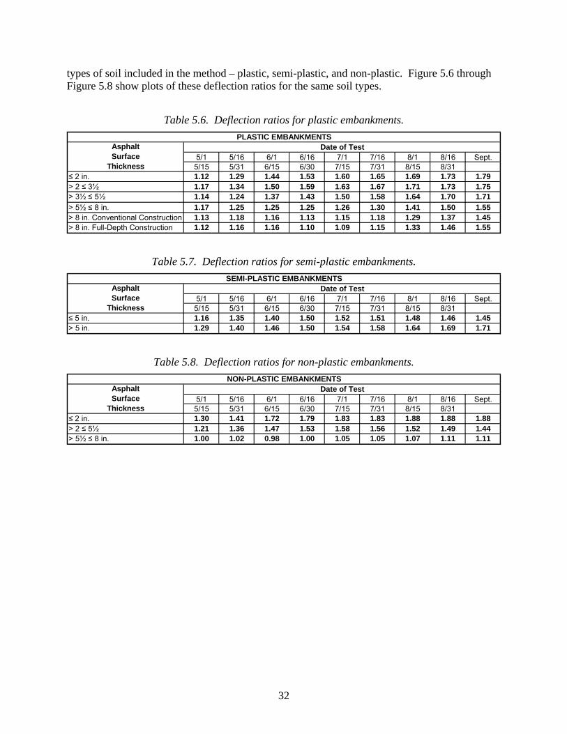
Deflection Ratio The deflection ratio adjustment factors in the TONN spring load capacity and flexible pavement overlays analysis methods are discrete values based on a range of dates and surface thicknesses. For the purposes of the thickness methodology development in this project, a linear regression analysis was conducted on the deflection ratio values for various soil types and surface thicknesses. The first step was to conduct the linear regression analysis for individual soil types, keeping the surface thickness constant. Table 5.6 through Table 5.8 provide the deflection ratios for the three
32
types of soil included in the method – plastic, semi-plastic, and non-plastic. Figure 5.6 through Figure 5.8 show plots of these deflection ratios for the same soil types.
Table 5.6. Deflection ratios for plastic embankments.
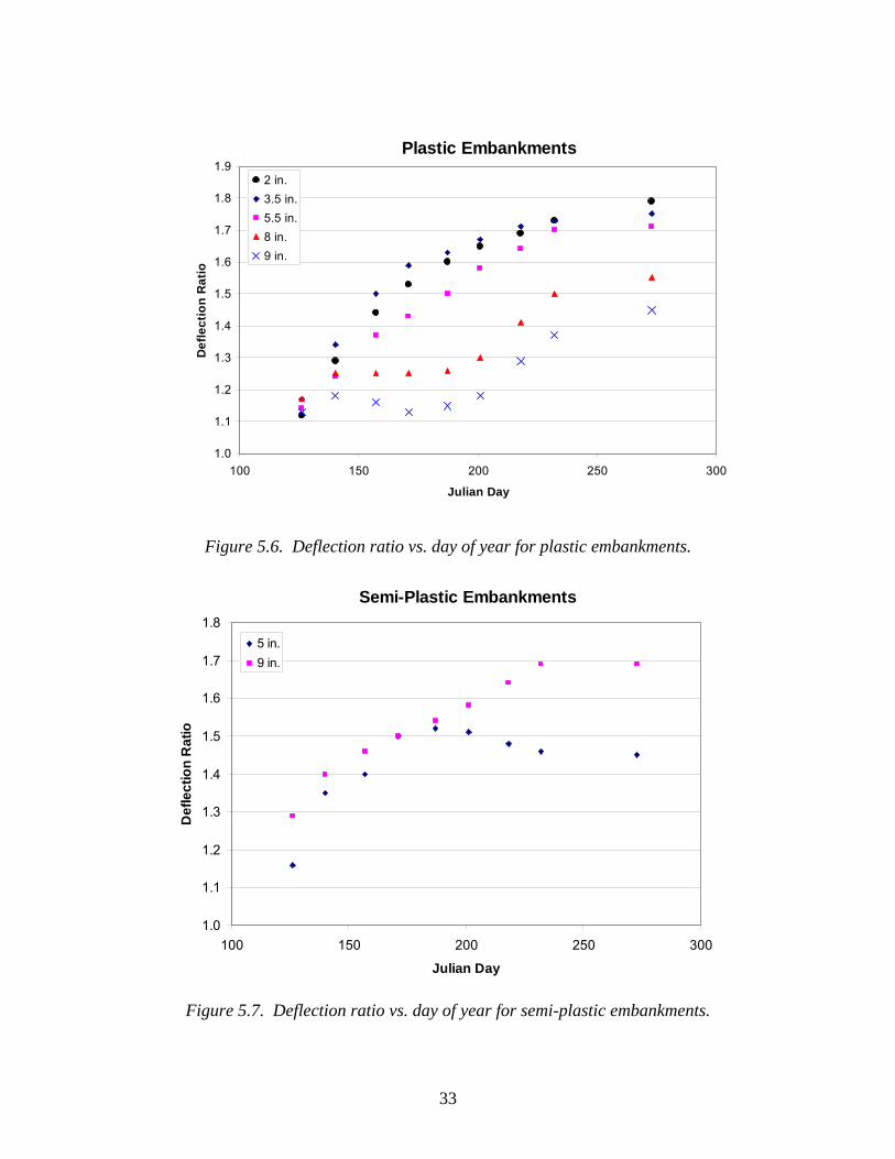
Figure 5.6. Deflection ratio vs. day of year for plastic embankments.
Semi-Plastic Embankments
1.0
1.1
1.2
1.3
1.4
1.5
1.6
1.7
1.8
100 150 200 250 300
Julian Day
Def
lect
ion
Rat
io
5 in.9 in.
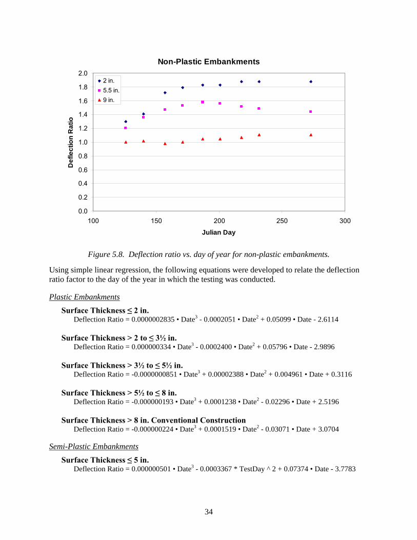
Figure 5.7. Deflection ratio vs. day of year for semi-plastic embankments.
34
Non-Plastic Embankments
0.0
0.2
0.4
0.6
0.8
1.0
1.2
1.4
1.6
1.8
2.0
100 150 200 250 300
Julian Day
Def
lect
ion
Rat
io2 in.5.5 in.9 in.
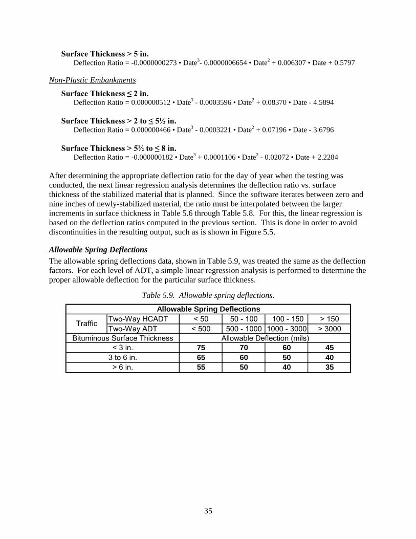
Figure 5.8. Deflection ratio vs. day of year for non-plastic embankments.
Using simple linear regression, the following equations were developed to relate the deflection ratio factor to the day of the year in which the testing was conducted.
Plastic Embankments
Surface Thickness ≤ 2 in. Deflection Ratio = 0.0000002835 • Date3 - 0.0002051 • Date2 + 0.05099 • Date - 2.6114 Surface Thickness > 2 to ≤ 3½ in. Deflection Ratio = 0.000000334 • Date3 - 0.0002400 • Date2 + 0.05796 • Date - 2.9896 Surface Thickness > 3½ to ≤ 5½ in. Deflection Ratio = -0.0000000851 • Date3 + 0.00002388 • Date2 + 0.004961 • Date + 0.3116 Surface Thickness > 5½ to ≤ 8 in. Deflection Ratio = -0.000000193 • Date3 + 0.0001238 • Date2 - 0.02296 • Date + 2.5196 Surface Thickness > 8 in. Conventional Construction Deflection Ratio = -0.000000224 • Date3 + 0.0001519 • Date2 - 0.03071 • Date + 3.0704
Semi-Plastic Embankments
Surface Thickness ≤ 5 in. Deflection Ratio = 0.000000501 • Date3 - 0.0003367 * TestDay ^ 2 + 0.07374 • Date - 3.7783
35
Surface Thickness > 5 in. Deflection Ratio = -0.0000000273 • Date3- 0.0000006654 • Date2 + 0.006307 • Date + 0.5797
Non-Plastic Embankments
Surface Thickness ≤ 2 in. Deflection Ratio = 0.000000512 • Date3 - 0.0003596 • Date2 + 0.08370 • Date - 4.5894 Surface Thickness > 2 to ≤ 5½ in. Deflection Ratio = 0.000000466 • Date3 - 0.0003221 • Date2 + 0.07196 • Date - 3.6796 Surface Thickness > 5½ to ≤ 8 in. Deflection Ratio = -0.000000182 • Date3 + 0.0001106 • Date2 - 0.02072 • Date + 2.2284
After determining the appropriate deflection ratio for the day of year when the testing was conducted, the next linear regression analysis determines the deflection ratio vs. surface thickness of the stabilized material that is planned. Since the software iterates between zero and nine inches of newly-stabilized material, the ratio must be interpolated between the larger increments in surface thickness in Table 5.6 through Table 5.8. For this, the linear regression is based on the deflection ratios computed in the previous section. This is done in order to avoid discontinuities in the resulting output, such as is shown in Figure 5.5.
Allowable Spring Deflections The allowable spring deflections data, shown in Table 5.9, was treated the same as the deflection factors. For each level of ADT, a simple linear regression analysis is performed to determine the proper allowable deflection for the particular surface thickness.
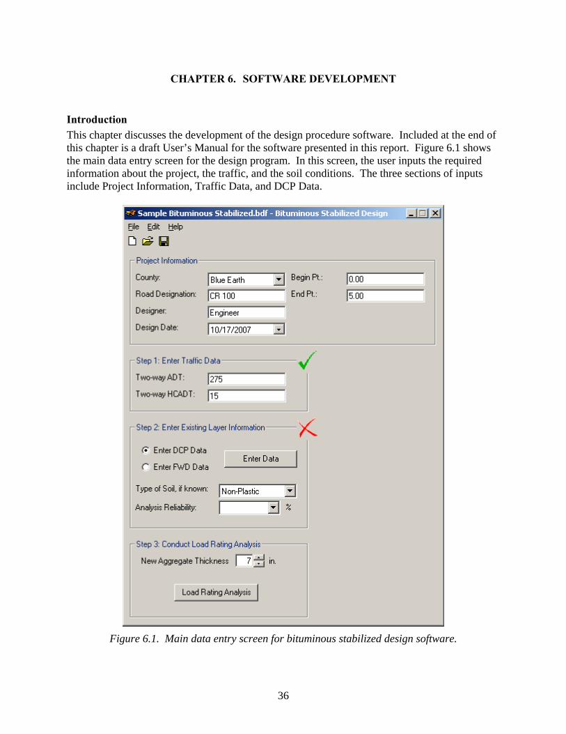
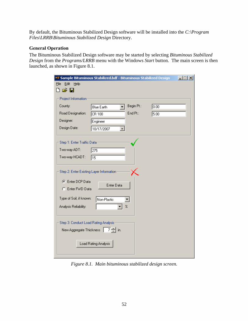
Introduction This chapter discusses the development of the design procedure software. Included at the end of this chapter is a draft User’s Manual for the software presented in this report. Figure 6.1 shows the main data entry screen for the design program. In this screen, the user inputs the required information about the project, the traffic, and the soil conditions. The three sections of inputs include Project Information, Traffic Data, and DCP Data.
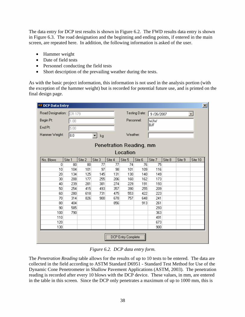
Figure 6.1. Main data entry screen for bituminous stabilized design software.
37
Project Information In this section, the basic information about the project is entered, including the following data.
• County name • Road designation • Beginning and ending point of the project (mileposts, reference points, or other
identifiers) • The name of the person developing the design • The date the design is completed
The information provided in this section does not affect the design calculations, but is printed in the in the design report, which is discussed in a later section.
Step 1: Enter Traffic Data The traffic data are entered in the “Step 1” area of the main screen of the software. In this area, the average daily traffic and the heavy commercial average daily traffic are entered. Since the design procedure does not require HCADT, the program allows users to enter an ADT but to leave the HCADT blank if desired. The values for ADT and HCADT are not limited in magnitude, but cautions have been placed to alert the user if potentially unreasonable values are entered. For example, the Mn/DOT Geotechnical and Pavement Manual (Mn/DOT, 1994) suggests upper limits for pavement thickness designs of ADT up to 750 and HCADT up to 60. In the program, if the user attempts to input a value exceeding these, a warning message window appears and asks if the user would like to keep the entered value or revise the number. The user may still enter values larger than those recommended, but will have been made aware of the potential discrepancy. Once acceptable values have been entered, the red X changes to a green check mark, indicating that the values have been validated and are acceptable, and will work in the design procedure.
Step 2: Enter Existing Layer Information In this step, the user can choose between entering DCP or FWD data. By choosing the appropriate option at the left of the window and pressing the “Enter Data” button, the DCP or FWD data entry window will appear. By selecting the “Enter DCP Data” option, the user can input data from up to 10 DCP tests from the roadway in question. Similarly, but selecting the “Enter FWD Data” option, the user can input the layer thickness and modulus values from backcalculated FWD data. The data entry will be addressed in the next section. The other two inputs are the type of soil and the reliability of the analysis. The type of soil is limited to broad categories of Plastic, Semi-Plastic, and Non-Plastic. These categories are based on the Mn/DOT TONN analysis, which is described in Chapter 5 of this report. The reliability is based on the average and standard deviation of the field test results. For the DCP results, once the stiffness values have been estimated as a result of the field testing, the average and standard deviation of those estimates are then used to determine the level of the stiffness values to use in the analysis. This assumes a uniform distribution of the test results and subsequent stiffness estimates.
38
The data entry for DCP test results is shown in Figure 6.2. The FWD results data entry is shown in Figure 6.3. The road designation and the beginning and ending points, if entered in the main screen, are repeated here. In addition, the following information is asked of the user.
• Hammer weight • Date of field tests • Personnel conducting the field tests • Short description of the prevailing weather during the tests.
As with the basic project information, this information is not used in the analysis portion (with the exception of the hammer weight) but is recorded for potential future use, and is printed on the final design page.
Figure 6.2. DCP data entry form.
The Penetration Reading table allows for the results of up to 10 tests to be entered. The data are collected in the field according to ASTM Standard D6951 - Standard Test Method for Use of the Dynamic Cone Penetrometer in Shallow Pavement Applications (ASTM, 2003). The penetration reading is recorded after every 10 blows with the DCP device. These values, in mm, are entered in the table in this screen. Since the DCP only penetrates a maximum of up to 1000 mm, this is
39
the maximum value allowed in the table. In addition, since the readings can only increase, the program checks for increasing values in the table cells. As can be seen in Figure 6.2, the final penetration reading does not need to correspond with a specific number of blows, since the number of blows is an indication of the stiffness of the soil layers below the surface. It is recommended that a minimum of two penetration tests be conducted for a roadway design. Preferably, 10 tests would be conducted per mile of roadway. As discussed in Chapter 5, each test only takes approximately 10 minutes, and an entire mile can be tested in less than two hours. Once the entry of the DCP data has been completed, the user must then press the “DCP Entry Complete” button, after which the data is saved and control is returned to the main screen. The FWD Data Entry screen reports the same basic information as the DCP Data Entry screen, with the exception of the hammer weight. The user is then asked for the thickness and resilient modulus of each layer, based on the results of backcalculated FWD testing. Once this information has been entered, the user can press the “FWD Entry Complete” button to return to the main screen.
Figure 6.3. FWD data entry form.
Step 3: Conduct Load Rating Analysis After all of the input data has been entered, and the validation shows that both steps 1 and 2 have been entered correctly, the user must select the thickness of new aggregate to be placed prior to
40
the stabilization. The allowable values are between 0 and 9 inches. Once this data is entered, the user can press the “Load Rating Analysis” button. This action will cause the final screen to appear – the results of the load rating analysis, which is a curve showing recommended spring load rating vs. stabilization thickness. This screen can be seen in Figure 6.4, below. The analysis will evaluate the allowable load rating with no additional gravel or stabilization, and will continue the evaluation through nine inches of stabilization, regardless of the additional gravel thickness input in Step 3. As shown in Figure 6.4, a plot of predicted load rating vs. stabilized depth is generated, with the project-related information supplied by the user at the top of the form. This screen can be printed in a single-page report for final design and approval purposes, as shown in Figure 6.5.
Figure 6.4. Results of load rating analysis.
41
Figure 6.5. Sample printed output from Bituminous Stabilized Design Software.
Conclusion This chapter described the software development effort for bituminous stabilized thickness design. The software is currently in a “beta” phase (Version 0.1), where it should be tested by
42
various users who will then report any problems to the developers. Once it has been tested (both programmatically, and technically) it can be considered to be in its release (Version 1.0) stage. Chapter 8 of this report contains a User’s Guide for the software, which can be printed separately from this report and used when testing and operating the software. This manual is a stand alone document, with repeats of the screens which have already been given in this chapter. It is written in a more direct and concise format, however, which is different than the language in the body of the report.
43
CHAPTER 7. CHARACTERISTICS AND ECONOMICS OF BITUMINOUS STABILIZED ROADWAYS
Stabilizing an aggregate-surfaced roadway can have several benefits, but it is not an appropriate strategy for every gravel road. The first part of this chapter describes the construction, maintenance, and rehabilitation of bituminous stabilized roadways, and their advantages and disadvantages. The remaining portions of this chapter discuss the characteristics of good candidates and the expected economic considerations for this type of construction. Not all low-volume, aggregate-surfaced roads are good candidates for bituminous stabilization as described in this report. There are several important factors to consider when determining the suitability of a particular roadway for this type of improvement. This chapter discusses these factors in two categories: characteristics and economics of good candidates for bituminous stabilized roadways.
Construction, Maintenance and Rehabilitation The construction, maintenance, and rehabilitation operations of bituminous stabilized gravel roads are similar, but have some differences. The expectations of performance should also be different. This type of upgraded gravel road is different than a roadway with a solid bituminous asphalt layer. This section describes the differences in construction, maintenance and rehabilitation, and reasonable performance expectations.
Construction The construction of a bituminous stabilized roadway is accomplished in several steps. Several of these steps have been discussed in previous sections of this report. The first step is to evaluate the existing roadway, using the techniques discussed in previous chapters. After determining the appropriate thickness of additional aggregate and the depth of bituminous stabilization, construction can begin. The additional aggregate is placed and compacted on top of the existing roadway surface. After this, the bituminous stabilization operation can be done. As de3scribed earlier, this can be done with a full-depth reclamation machine, set at the appropriate depth. After the reclamation machine makes its pass, the stabilized material must be recompacted using pneumatic and steel drum rollers. The stabilized surface must then be allowed to cure for approximately two weeks, where no heavy vehicular loads are placed on the roadway during this time. After the stabilization construction, and after the material has been allowed to cure properly, at least one seal coat must be placed on the surface. Two seal coats (one soon after construction and one at the beginning of the following construction season) are recommended.
Maintenance In general, the maintenance activities required for this type of roadway are similar to those for other low-volume roads with bituminous pavements. Cracks should be sealed, and shoulders maintained. The seal coat at the surface, which protects the stabilized material from degradation, must be carefully observed and maintained whenever needed.
44
Special attention should be paid to permanent deformations that may become evident in the surface. The rutting cause by these permanent deformations can be detrimental in several ways. Not only is this type of distress indicative of potential failures in the surface or underlying layers, it can also contribute to further damage to the surface when the snow is plowed in the winter. When rutting becomes moderate to severe, snow plows can scrape the important seal coat from the surface. When this occurs, the newly exposed stabilized material becomes less resistant to degradation, and the surface can begin to ravel. If an additional seal coat is not applied to the surface soon after it is damaged by snow plows, the degradation may require more extensive maintenance and perhaps rehabilitation activities.
Rehabilitation Several options exist for rehabilitation of bituminous stabilized roadways. Although this type of pavement upgrade is normally only placed on very low volume roads, distresses such as cracking and rutting may become evident, and need rehabilitation. One option for rehabilitating this type of roadway is to plan for its eventual upgrade to a bituminous pavement from the time of initial construction. When traffic exceeds a level determined by the agency, the roadway should be programmed for upgrade to bituminous pavement, using the existing stabilized layer as a stiff base. The roadway can then be maintained as a bituminous pavement from that time forward. A second option is to maintain the roadway as a bituminous stabilized surface with a seal coat cover. The seal coat should be updated at regular intervals, depending on the surface condition. If this option is selected for rehabilitation of this type of roadway, the agency must recognize the potential for rutting in the bituminous stabilized layer, and should carefully observe the progression of any rutting that may occur. The rutting by itself is not a large problem, but it increases the probability that snow plows in the winter will scrape off the seal coat layer, causing additional damage when the surface thaws. A third option is not to conduct any rehabilitation activities on the roadway at all. After the initial seal coats have been deteriorated, the roadway surface will slowly return to a type of gravel roadway. One drawback of this method is that the benefits of stabilization are quickly lost. In addition, the public quickly becomes accustomed to a smoother road surface and would not tolerate a poor road surface.
Benefits of Bituminous Stabilization There are several benefits to stabilizing gravel roads with an asphalt emulsion. These benefits include the following.
• Improvements to the driving surface and in safety • Virtual elimination of dust problems • Reduction in the loss of aggregate • Reduction of maintenance and regrading costs • Relatively inexpensive method of upgrading a gravel roadway
45
Improvements to Driving Surface A particular advantage to bituminous stabilization is that the driving surface is greatly improved. The gravel surface is effectively bound with the asphalt emulsion, and with one or two seal coat layers after the stabilization process, the surface roughness is greatly reduced. In addition, the probability of airborne gravel particles striking a vehicle while driving behind another vehicle is greatly reduced. There are some disadvantages to this improved driving surface, which will be discussed in a following section.
Elimination of Dust By binding the aggregate with asphalt emulsion, the dust that is normally associated with an aggregate-surfaced road is virtually eliminated. In addition to the elimination of dust, this also means that mud is eliminated during rain events.
Reduction in Loss of Aggregate Another benefit to binding the surface layer with asphalt emulsion is that the aggregates in the surface are not lost in the ditches and are less likely to degrade and be crushed due to the action of vehicle tires and of the environment. The loss of aggregate is one of a highway agency’s major expenditures for roadway maintenance of aggregate surfaced roads. The clear benefits to dramatically reducing the amount of lost aggregates include cost savings as well as using less of a limited resource that seems to be getting more and more difficult to find. Associated with the reduction in the loss of aggregate is a savings in maintenance and regrading costs. Although there are some expenses that must be made to maintain the surface integrity, such as periodic seal coats and observations to ensure that rutting does not become excessive.
Potential Disadvantages to Bituminous Stabilization While there are many benefits to upgrading a gravel roadway with bituminous stabilization, there are also some disadvantages that must be considered. These include the following.
• Potential to induce higher driving speeds and thus, potentially dangerous curves in existing geometry
• Potential distresses
Higher Speeds A better driving surface normally induces drivers to increase speeds on a roadway. The dramatic difference in pavement smoothness and surface texture are a great benefit to drivers. However, a highway agency must take the potential for increased driving speeds into consideration. It is unlikely that the relatively inexpensive bituminous stabilization of aggregate surfaced roadways will be accompanied by major changes to the roadway geometry. If the geometry remains the same, existing curves in the roadway geometry have the potential to become dangerous. In general, highway agencies that have used this method have not added striping to the roadways, for the express purpose of avoiding the appearance that the newly stabilized roadway has been improved in any other way. The roadway still has its existing features, which may include limited width, potentially inadequate drainage characteristics, lack of clear lanes, and
46
other conditions which would make it unsuitable for striping and the appearance of a roadway designed for higher speeds.
Potential Distresses Although the process of bituminous stabilization is fairly straightforward, there are some conditions which can cause certain distresses to have an adverse effect on the performance of the pavement. As discussed previously in this chapter, the stabilized layer may experience rutting over a period of several years, which may lead to unintended consequences later in the winter when snow is cleared by plows. The blade of the snow plow may peel off the protective seal coat in some places on the surface of the stabilized layer, which exposes the stabilized material to accelerated deterioration. When this occurs, it is normally in the center or edges of the roadway, near the high points left by the rutting. This type of distress occurred on CR 163 in Blue Earth County, which was stabilized in 2002. Subsequent seal coats may not always be able to be placed in a timely manner to restore the surface and replace the protective features, and additional deterioration may occur. At the extremes, this type of damage may require a bituminous overlay on the surface of the stabilized material. County Road 163 received this type of rehabilitation in 2007.
Characteristics of Candidate Projects There are several characteristics that a good candidate for bituminous stabilization should exhibit. When selecting a candidate road, the highway agency should consider the following.
• ADT • Geometry • Width • Proximity to Development • Potential for future upgrade needs
In general, the average daily traffic on a candidate roadway should not exceed approximately 200 vpd. The geometry of the roadway should be considered in determining the suitability of a candidate roadway. The presence of relatively sharp curves, as discussed above can be a deterrent to selecting a particular roadway for bituminous stabilization. The width of the roadway should also be considered. With potentially increased speeds, and possibly increased traffic as well, roadways that are more narrow may present future traffic problems. The proximity of the roadway to developed areas, and the associated potential for future upgrades, should also have an impact on its selection for bituminous stabilization. Roadways that are closer to developments will likely need to be upgraded nearer in the future than others. It is suggested that counties take the potential for future upgrade needs and the likelihood of increased traffic into consideration when stabilizing roadways in this manner.
Expectations Many typical considerations for deciding a stabilize a gravel roadway with bituminous emulsion have been discussed previously. It is important to be realistic in the expectations of a bituminous stabilized roadway. This type of roadway upgrade is not a bituminous surface, nor is it expected
47
to perform at a significantly higher level than the gravel roadway from which it was constructed. The primary reasons for considering a bituminous stabilized roadway are to reduce the loss of aggregate, improve the driving surface, and to eliminate dust. The potential distresses discussed in previous sections (rutting and snow plow damage) are real possibilities, and must not be ignored in the cost analysis when deciding on this type of construction. Other reasonable expectations include the necessity for common maintenance items similar to a bituminous pavement, including periodic seal coats. Sealing cracks is likely not a necessity, but can be performed if the agency desires. Currently, fatigue life has not been considered, since the purpose of bituminous stabilization is for cost savings and other incidental improvements to the surface. It is thought that these surfaces will last as long as their gravel-surfaced counterparts, but with the increased performance in terms of riding surface and lower maintenance and rehabilitation costs.
Economics There have been several research projects funded by Minnesota transportation agencies and others to study the economic impacts, needs, and other aspects of pavements, and in the topic of upgrading gravel roads in particular. Some of these include Jahren, et al., 2005; Skok, et al., 2002; Forsberg, 1997; and Beaudry, 1992. This section presents some of the information included in the report “Economics of Upgrading and Aggregate Road”, authored by Jahren, et al., and published by the LRRB in 2005 (hereafter called the “Iowa State” report). This section adds parallel components to the results in that report relating to the bituminous stabilization of gravel roads. As discussed in the Iowa State report, only those activities related to the specific surface type are included in the economic analysis presented here. These include:
Since the Iowa State report presented information on gravel- and bituminous-surfaced roads, this report will focus on the maintenance and construction costs for bituminous stabilized roadways, and will make basic comparisons between the average annual cost for these types of roads and those discussed in the Iowa State report. In the previous report, the annual costs based on a five-year re-graveling cycle for gravel roads and a seven-year resurfacing cycle for bituminous roads, were presented for roadways with ADT in the 100-200 vehicles per day range. This level was chosen by the authors of the Iowa State study because gravel roads that are normally upgraded to bituminous surfaces usually fall into this ADT range.
48
The ADT range for most gravel roads in Blue Earth County, where the bituminous stabilization construction described in this report took place, is in the 50-100 vpd range, and it is recommended that gravel roadways not be bituminous-stabilized if the ADT exceeds 200 vpd. Since the ADT ranges for the Iowa State study and for the bituminous stabilized roadways in this report are similar, the average annual cost values can be compared more reliably. The average annual expenditures for gravel roads with a 5-year re-graveling cycle were reported to be about $4,160 per year per mile. This value includes annual grading and other annual maintenance of the surface ($1,400 per mile per year, including re-graveling years), and re-graveling every five years ($13,800 per mile). For bituminous surface roads, with a 7-year resurfacing cycle, the expenditures were about $2,460 per year per mile. This value includes annual maintenance ($1,600 per mile per year, including seal coating years) and seal coating every seven years ($6,000 per mile). The report also assumes that when a gravel road is upgraded to a bituminous surface, the cost is about $130,000 per mile. Using the same expenditure categories for the bituminous stabilized roadways in Blue Earth County (CR 163 and CR 179, which were both constructed in 2002) the average annual maintenance expenditures are about $363 per year, per mile (not including a large expenditure at a fixed time interval). This is, however, based on only three years of data. County Roads 118 and 172 were constructed in 2005, and were not included in the annual expenditures calculation. After five years in service, the bituminous stabilized surface on CR 163 required more than just another seal coat to repair damage that had been done by snow plows during the winter (see the discussion of this type of distress in a previous section of this chapter). Construction of the bituminous stabilized layer on CR 163 and CR 172, in 2002, and on CR 118 and CR 179 in 2005, was $117,600 per mile, not accounting for inflation. The one-inch overlay that was placed on CR 163 could be considered a step in the direction of full bituminous surfacing. A county may utilize this step in a planned conversion to a bituminous roadway. The cost of this one-inch overlay on the bituminous-stabilized surface was $44,906 (2007 dollars) per mile over a 2.5-mile section. This is approximately one-third of the $130,000 (2004 dollars) average cost of upgrading a gravel road to a bituminous surface. Another option that could have been chosen would be to apply another seal coat to the surface to determine if this would restore the surface protection to the bituminous stabilized layer. As described in the Iowa State report, the seal coat would cost approximately $7,600 per mile in 2004 dollars. It is difficult to determine the average annual cost for bituminous surfaced roadways in terms of annual maintenance and long-interval repair. While this cost may be as low as $1,961 per mile per year (considering a seal coat every five years), it may need to be considered on a different schedule, in terms of a 5-10 year transition to a bituminous-surfaced roadway (although the other considerations, discussed previously in this chapter, would still apply). Figure 7.1 shows the annual maintenance and upgrade costs for four options – maintain gravel surface, bituminous stabilized, upgrade to HMA, and staged upgrade to HMA. The staged upgrade to HMA includes first stabilizing the gravel road in the manner discussed in this report, adding a 1- to 1½-inch overlay at year 5, and then repeating the overlay operation seven years
49
later. It must be noted that the estimates for bituminous stabilization are based on very limited data and maintenance schedules. It is likely that the bituminous stabilized surface may require the staged upgrade to HMA method, rather than continuing as a bituminous stabilized surface with a seal coat application every five years.
0
50
100
150
200
250
0 5 10 15 20 25Years
Cos
t ($1
000s
)
Remain Gravel
Bituminous StabilizationUpgrade to Bituminous
Staged Bituminous
Figure 7.1. Costs per mile for various maintenance / upgrade options.
It is apparent in Figure 7.1 that the cost of the “maintain gravel” option will eventually exceed the cost of the other options with the exception of the “staged bituminous”. While it may take several decades for the financial benefits of either two lower-cost options to become apparent, the other benefits of bituminous stabilization or upgrading to HMA must be considered when making decisions of this type. The associated potential long-term effects, such as safer, smoother, dust-free roadways should be considered. For roads where the ADT is not expected to increase over the 100 to 200 vpd range in the future, the bituminous stabilization method may be the appropriate choice, although a longer history with maintenance and rehabilitation costs and schedules is certainly needed. To continue the similarities in the analysis with those of the Iowa State report, the average annual cost for the maintenance and 5- or 7-year rehabilitation schedule were computed. In the Iowa State report, the average annual cost of HMA and gravel maintenance, for counties in Minnesota, was estimated at $2,460 and $4,160 per year per mile. Computed in the same
50
manner, the average annual cost of bituminous stabilized and staged-bituminous upgrade was estimated to be $1,362 and $5,196 per year per mile. Again, these two estimates are based on just three years of maintenance cost data, and only one rehabilitation interval. In Figure 7.2, the straight lines added to the accumulated costs from Figure 7.1 indicate the annual maintenance and rehabilitation costs (after initial construction costs). The slopes of these lines are noted next to each in the figure.
0
50
100
150
200
250
0 5 10 15 20 25
Years
Cos
t ($1
000s
)
Bituminous Stabilization
Remain GravelUpgrade to Bituminous
Staged Bituminous
$4,160 /yr/mi
$1,360 /yr/mi
$2,460 /yr/mi
$5,200 /yr/mi
Figure 7.2. Average annual maintenance and rehabilitation costs per mile.
51
CHAPTER 8. SOFTWARE USER’S MANUAL
Bituminous Stabilized Design for Gravel Roads Version 0.1
Introduction Bituminous Stabilized Design is an engineering software application that allows users to determine the most appropriate stabilization depth for a roadway using asphalt emulsion in a full-depth reclamation style construction method. Users can enter field testing data and other pertinent inputs and save the information in a “Bituminous Stabilized Design” file (*.bdf file extension). After a stabilization depth analysis has been performed, the results may be printed in a report format that can be used for design approval and verification.
System Requirements Bituminous Stabilized Design has been developed for computer systems that meet the following requirements: Operating Systems
• Windows 2000 with Service Pack 3, or • Windows XP Professional
Installation The following steps are required to install the Bituminous Stabilized Design software.
• Close all running applications, since the installation may need to reboot the computer. • Insert the Bituminous Stabilized Design CD-ROM into the CD drive of the computer
Or Extract the Bituminous Stabilized Design files from the downloaded zip file to a new temporary folder.
• If using a CD, the setup program should launch automatically. If not, click on the Windows Start button, choose Run, and type D:\Setup.exe (where D:\ is the drive letter of the CD drive.)
• If the installation files were downloaded directly to your computer, move to the folder where the files were extracted and double-click the Setup.exe file.
• Follow the instructions in the installation application. • If the installation application informs you that a newer file already exists on your
computer, choose to keep the current file, and do not overwrite a newer file with an older one.
52
By default, the Bituminous Stabilized Design software will be installed into the C:\Program Files\LRRB\Bituminous Stabilized Design Directory.
General Operation The Bituminous Stabilized Design software may be started by selecting Bituminous Stabilized Design from the Programs/LRRB menu with the Windows Start button. The main screen is then launched, as shown in Figure 8.1.
Figure 8.1. Main bituminous stabilized design screen.
53
Starting a New Analysis File By selecting the File/New menu item, all information in the main screen and all subsequent screens will be deleted and a new file can be saved with new data. If unsaved data exists from a previous file, the user will be prompted to save the data. A new file can also be started by pressing the New toolbar button.
Opening Analysis Files Analysis files can be opened by various methods. The software will only open one analysis file at a time, which can be done by selecting the file in Windows Explorer and either double-clicking the filename or by pressing the Enter key. BDF files can be opened in this manner. Within the Bituminous Stabilized Design software, analysis files may be opened by selecting the File/Open… menu item and selecting the file from the file open dialog box. This can also be done by pressing the Open toolbar button. If the open menu item is selected when a previous analysis has not yet been saved, the user is prompted to save the previous file prior to continuing with the File/Open command.
Saving Analysis Files To save the current analysis file, select the File/Save As… or File/Save menu item. Save As… is used to give the file a new name, and Save is used to save the analysis file under its current name. This can also be accomplished by pressing the Save toolbar button.
Application Options Options specific to the Bituminous Stabilized Design software can be accessed by selecting the Edit/Options… menu item. The options screen will appear, as shown in Figure 8.2.
Figure 8.2. Application options screen.
54
Default File Location
This setting allow the default data file location to be set. By providing a default file location (select the file location in the list box below the File Locations text) , the software will look there first when opening and saving files.
Default County
By selecting a default county, the user will not be required to select a county in the main software screen each time an analysis is conducted. The default county will already be highlighted in the Project Information area.
Exit Bituminous Stabilized Design To exit the software, select the File/Exit menu item. If unsaved data exists in the software, the user is prompted to save the information prior to exiting.
Conducting an Analysis To conduct a design analysis, three steps must be completed in addition to entering the basic project information. These are
• Enter Traffic Data • Enter Existing Layer Information • Conduct Load Rating Analysis
Step 1 – Enter Traffic Data The user is prompted to enter traffic data by typing the values for Two-way ADT and Two-way HCADT. While only the ADT is necessary for the analysis, if HCADT data is entered, it will be used rather than ADT. Once at least ADT is entered correctly, with an integer value greater than 0, the red X icon in the upper right corner of the Step 1 frame turns to a green check.
Step 2 – Enter Existing Layer Information The information to define the existing layers is based on either Dynamic Cone Penetrometer or Falling Weight Deflectometer data. Depending on the field testing method chosen by the user, the Enter DCP Data or Enter FWD Data option is selected. The user then presses the Enter Data button, after which control of the program is transferred to the field data entry screen, as shown in Figure 8.3 and Figure 8.4, respectively. In addition to the DCP or FWD data entry, the user is asked to enter the type of soil, if known (default is Plastic) and the analysis reliability requested. This option is only available if the DCP data is selected, since the results from multiple DCP tests can be averaged and the level or reliability in the layer information can be estimated.
DCP Data Entry
If the user elects to enter data using DCP field test results, the screen shown in Figure 8.3 appears. The same information from the Project Information frame is repeated here, with additional information specific to the DCP testing requested of the user.
55
Figure 8.3. DCP data entry screen.
The actual DCP data is entered in the data grid. The data for each DCP test is entered, with the initial reading and a reading after every subsequent 10 blows with the DCP hammer. Once this data is entered, the user can press the DCP Entry Complete button to return to the main screen.
FWD Data Entry
Similar to the DCP data entry, if the user elects to enter data acquired from FWD testing, the FWD Data Entry screen appears after pressing the Enter Data button in the main screen. Again, the basic project information is repeated in the FWD data entry screen, with a request for additional data specific to the FWD testing.
56
Figure 8.4. FWD data entry screen.
The layer information entered here is a result of FWD backcalculation, and consists only of the existing layer thickness and resilient modulus. Once this data is entered, the user can press the FWD Entry Complete button to return to the main screen.
Step 3 – Conduct Load Rating Analysis In this step, the user selects the quantity of additional new gravel to be analyzed, and then presses the Load Rating Analysis button. The load rating analysis takes all the information provided by the user and conducted a series of 10 analyses – one for each stabilized depth (0 through 9 inches). After performing the analysis, the software opens the Load Rating Analysis screen, as shown in Figure 8.5. This screen repeats all the basic project data entered by the user, and displays a graph of the results of the ten analyses. The graph shows the results in terms of load rating (tons) vs. stabilized depth (inches).
57
Figure 8.5. Load rating analysis screen.
The user is presented with two buttons in this screen – Print and Close. By selecting the Close button, control of the software is returned to the main screen, from which another analysis may be conducted with modified data, or the file may be saved or closed.
Printing Results By pressing the Print button in the Load Rating Analysis screen, the user may print the results to a paper printer. The user is presented with a standard print window from Microsoft Windows, similar to that shown in Figure 8.6 (though the list of available and active printers may be different on each system). After selecting an available printer, and pressing the Print button, a single page will be produced, which contains the same information as the Load Rating Analysis screen. In addition to this information, and the graph of results, four additional lines are added at the bottom of the page. The first two of these are the final recommended additional gravel and the recommended stabilization depth, based on the analyses conducted. The last two lines are for signatures and dates of the recommendation and approval for the design.
58
Figure 8.6. Standard print screen.
59
CHAPTER 9. CONCLUSIONS AND RECOMMENDATIONS
This chapter provides a review of the design procedure for bituminous stabilized roadways developed as part of this project, and discusses recommendations for additional research and for implementation.
Review of Design Procedure The design procedure for determining the required depth of bituminous stabilization in gravel roads was described in this report. The development of the procedure included the characterization of the materials involved – underlying soils, unbound aggregate, and stabilized material, field construction to determine in-situ properties of the materials, modification of existing analysis methods, and software development to automate the design. From the pavement designer’s perspective, the thickness design method uses the software package developed as part of this project, and described in this report. A user’s manual is provided in Chapter 8 of this report. The designer must obtain DCP test results conducted at regular intervals along the roadway in question, and enter these results into the software. In addition to this information, basic ADT, HCADT, and soil type information must be provided by the engineer. At this point, the designer must select the level of reliability desired, and the amount of new aggregate to be analyzed as a starting point. By pressing the “Load Rating Analysis” button, the designer is provided an estimate of the required depth of bituminous stabilization for increasing allowable load ratings.
Conclusions This report presents the basis for a new design method for the thickness of a bituminous stabilized layer constructed on an existing aggregate surfaced roadway. The method requires the input of properties and thicknesses of existing layers, and then uses layered elastic theory to predict the deflections at the surface after a stabilized layer is placed. The research reported in this report currently uses relationships between DCP index and resilient modulus and between DCP index and backcalculated FWD moduli. Due to the inherently variable nature of fine- and coarse-grained soils, the results of these correlations may not be the most appropriate for the use intended. This method of improving aggregate-surfaced roadways has several benefits, including the following:
• Improvement in ride quality, surface roughness, and safety • Virtual elimination of dust problems • Reduction in the loss of aggregate • Reduction of maintenance and regrading costs • Relatively inexpensive method of upgrading a gravel roadway • Conservation of future maintenance and construction funds as well as natural resources
due to dramatically decreased regrading and reshaping needs.
60
There are some possible disadvantages to improving a roadway with this method, including the unintended result of providing a better driving surface – higher speeds. Many aggregate-surfaced roadways are not designed geometrically for higher speeds, and the potential for a false sense of security exists, by driving on a smoother, harder surface. Another potential disadvantage is the possibility for rutting in the surface and the adverse effects of snow plows on the seal coats at the surface which are important to maintaining the integrity of the bituminous stabilized layer. From a materials standpoint, there remain several limitations in the design method. A major limitation at this time is the minimal amount of empirical data to support the correlations between DCP and MR and between FWD and MR. Another limitation is that the data used in the TONN load rating analysis uses spring thaw conditions in some of the factors for determining the load rating. These factors would be useful in northern tier states where spring thaw is a major issue.
Recommendations for Additional Research There are several aspects of this research which should be continued in order to improve the design procedure and to make it more reliable. These include the following.
• The sensitivity of the design method to different types and manufacturers of water-based emulsions should be investigated. The current research only used one source and type of emulsion.
• The models used for correlating DCP index with resilient modulus should be evaluated. If necessary, these models should be modified, calibrated, or simply replaced with others using various soils found in the upper Midwest region.
• When the updated TONN model is available, it should be considered for use in the design method.
• Additional test sites, for validation, should be evaluated. This additional data will allow the procedure to be validated.
• The fatigue characteristics of the stabilized layer and the definition of failure in such a pavement structure should be investigated. The information from the four construction sites in Blue Earth County can be used as a starting point for this work.
Recommendations for Implementation In order for a county engineer or other pavement design professional to implement this design method, several items should be considered. Initially, the thickness of additional gravel and the stabilized depth should be compared to other methods and the engineer’s own judgment to validate or reinforce the results of the design procedure. Some of the items that a pavement design engineer may consider evaluating in order to become comfortable with the design procedure include the following.
• Effect of DCP and FWD results, as well as soil type, on additional gravel thickness and stabilization depth.
• Recommended additional gravel thickness and stabilization depth for several designs as compared to previous designs and the engineer’s judgment.
61
• Sensitivity of the design recommendations to traffic levels (ADT and HCADT) and other inputs.
• Comparison of historical, local costs between bituminous stabilization, upgrading to bituminous pavement, or leaving the roadway surface gravel. These comparisons should be conducted similar to the examples given in Chapter 7.
On a statewide level, the implementation of this design method will depend on county and other engineers using it and sharing their experiences with others. As more engineers become familiar and comfortable with the concept and process of bituminous stabilization, and with the design method, others will be induced to try it and evaluate the costs and benefits for themselves. Another aspect that will affect the statewide implementation of this process and the method is the long-term experiences of engineers with the maintenance and rehabilitation requirements of roadways constructed in this way. If the seal coat schedule and potential overlay requirements after several years cause the costs to increase significantly, the other benefits to this construction method may be overcome by the costs.
62
REFERENCES
Beaudry, T., Minnesota’s Design Guide for Low Volume Aggregate Surfaced Roads, Report No. MN/RD-92/11, Minnesota Local Road Research Board, St. Paul, Minnesota, 1992. Skok, E., D. Timm, M. Brown, and T. Clyne, Best Practices for the Design and Construction of Low Volume Roads, Report No. MN/RC-2002-17, Minnesota Local Road Research Board, St. Paul, Minnesota, 2002. Erickson, H and A. Drescher, The Use of Geosynthetics to Reinforce Low Volume Roads, Report No. MN/RC-2001-15, Minnesota Department of Transportation, St. Paul, Minnesota, 2001. Kruse, C.G. and E.L. Skok, Flexible Pavement Evaluation with the Benkelman Beam, Minnesota Department of Highways, Investigation 603 Summary Report, St. Paul, Minnesota, 1968. Forsberg, A.T., Blue Earth County Finn/Oil Gravel Project, Minnesota Department of Transportation, Report No. MN/RC-97/12, St. Paul, Minnesota, April 1997. Bushman, W., T. Freeman, and E. Hoppe, Stabilization Techniques for Unpaved Roads, Report No. VTRC 04-R18, Virginia Transportation Research Council, Charlottesville, Virginia, 2004. Jahren, C. T., D. Smith, J. Thorius, M. Rukashaza-Mukome, and D. White, Economics of Upgrading an Aggregate Road, Report No. MN/RCD – 2005-09, Iowa State University, Ames, Iowa, 2005. Lunsford, G. and J. Mahoney, Dust Control on Low Volume Roads: A Review of Techniques and Chemicals Used, Report No. FHWA-LT-01-002, University of Washington, Seattle, Washington, 2001. Skorseth, K., and A.A. Selim, Gravel Roads Maintenance and Design Manual, South Dakota Local Transportation Assistance Program, Report No. LTAP-02-002, April, 2005. AASHTO Guide for the Design of Pavement Structures, AASHTO, Washington, DC, 1993. American Society of Testing Materials, Standard Test Method for Use of the Dynamic Cone Penetrometer in Shallow Pavement Applications, ASTM D6951-03, ASTM International, West Conshohocken, Pennsylvania, 2003. George, K.P., Waheed Uddin, Subgrade Characterization For Highway Pavement Design, Final Report Mississippi Department of Transportation, Vicksburg, Mississippi, 2000. Mn/DOT Geotechnical and Pavement Manual, Minnesota Department of Transportation, St. Paul, Minnesota, 1994.