Page 1
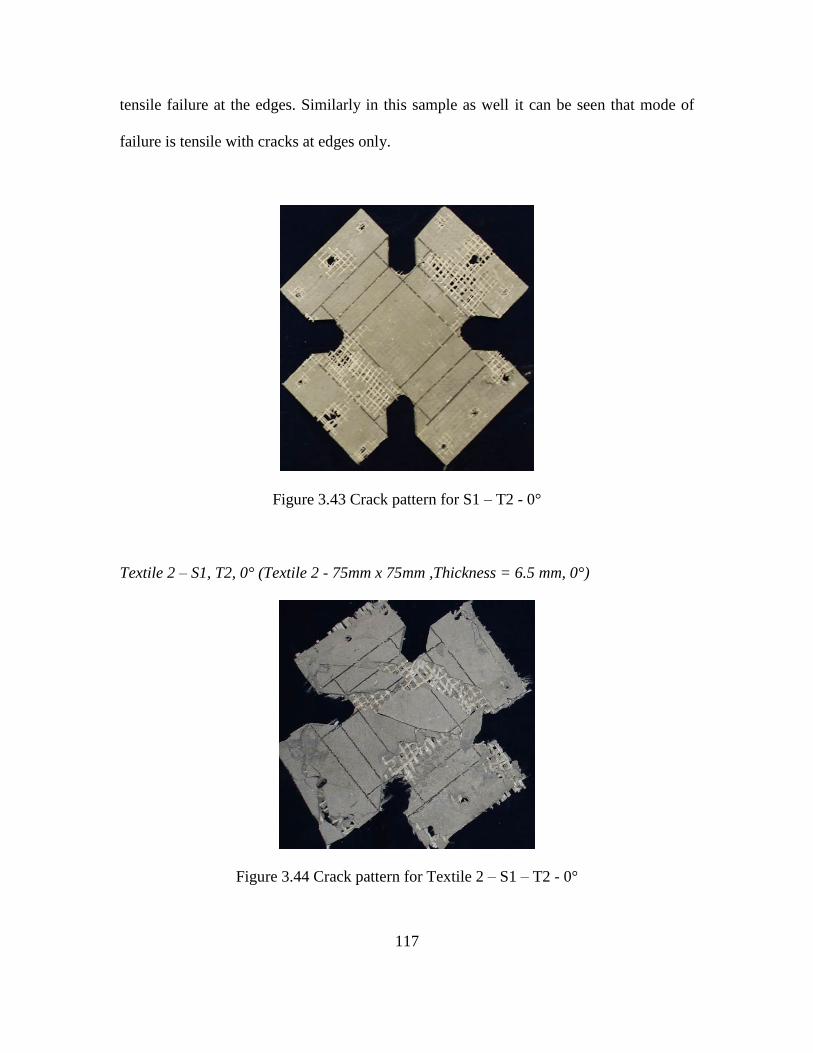
Design procedures for Strain Hardening Cement Composites (SHCC) and measurement of their
shear properties by mechanical and 2-D Digital Image Correlation (DIC) method
by
Karan Aswani
A Thesis Presented in Partial Fulfillment
of the Requirements for the Degree
Master of Science
Approved April 2014 by the
Graduate Supervisory Committee:
Barzin Mobasher, Chair
Subramaniam Dharmarajan
Narayanan Neithalath
ARIZONA STATE UNIVERSITY
May 2014
Page 2
i
ABSTRACT
The main objective of this study is to investigate the behaviour and applications of strain
hardening cement composites (SHCC). Application of SHCC for use in slabs of common
configurations was studied and design procedures are prepared by employing yield line
theory and integrating it with simplified tri-linear model developed in Arizona State
University by Dr. Barzin Mobasher and Dr. Chote Soranakom. Intrinsic material property
of moment-curvature response for SHCC was used to derive the relationship between
applied load and deflection in a two-step process involving the limit state analysis and
kinematically admissible displacements. For application of SHCC in structures such as
shear walls, tensile and shear properties are necessary for design. Lot of research has
already been done to study the tensile properties and therefore shear property study was
undertaken to prepare a design guide. Shear response of textile reinforced concrete was
investigated based on picture frame shear test method. The effects of orientation, volume
of cement paste per layer, planar cross-section and volume fraction of textiles were
investigated. Pultrusion was used for the production of textile reinforced concrete. It is an
automated set-up with low equipment cost which provides uniform production and
smooth final surface of the TRC. A 3-D optical non-contacting deformation measurement
technique of digital image correlation (DIC) was used to conduct the image analysis on
the shear samples by means of tracking the displacement field through comparison
between the reference image and deformed images. DIC successfully obtained full-field
strain distribution, displacement and strain versus time responses, demonstrated the
bonding mechanism from perspective of strain field, and gave a relation between shear
angle and shear strain.
Page 3
ii
ACKNOWLEDGEMENTS
I would like to specially thank my advisor Dr. Barzin Mobasher, who provides me the
opportunity to work in the field of research that I could go through variety of excited
topics and experimental programs. Let alone all the attention, invaluable intellectual
insights he gave me. I also want to extend my appreciation to Dr. Subramaniam D. Rajan
and Dr. Narayanan Neithalath who served as my committee members, helping and
supervising my progress in Master’s degree program.
I would also like to thank Vikram Dey, who actually taught me many skills including
preparing and conducting experiment, data analysis and all of his supports and ideas
throughout my research work. Outstanding work done by my peers, Dr. Deju Zhu and Dr.
Chote Soranakom established the basis and a straight forward path that I could follow up
and extended my work to further areas.
I greatly appreciate the assistance provided by Mr. Peter Goguen and Mr. Kenny Witczak
for all of their great works in the laboratory, especially the trouble-shooting and
maintenance on testing devices. Without their help, I could definitely not finish my
experiments.
Absolutely, I would express my gratitude to my dear colleagues and friend, Yiming Yao,
Robert Kachala and Xinmeng Wang for their help and more importantly, the great time
we spent together.
Page 4
iv
TABLE OF CONTENTS
CHAPTER Page
LIST OF FIGURES .......................................................................................................... vii
LIST OF TABLES ............................................................................................................ xii
CHAPTER 1 - INTRODUCTION .......................................................................................1
1.1 Overview ...............................................................................................................1
1.1.1 Strain Hardening Cement Composite ..........................................................2
1.1.2 Textile Reinforced Concrete as a Strain Hardening Cement Composite .....2
1.1.3 Materials ......................................................................................................4
1.2 Simplified Strain-hardening Cement composites (SHCC) Model ........................5
1.2.1. Derivation of Moment-Curvature Capacity ..........................................................8
1.3 Production Techniques ........................................................................................15
CHAPTER 2 - LIMIT STATE ANALYSIS OF STRAIN HARDENING STRUCTURAL
PANELS…. .......................................................................................................................18
2.1 Yield Line Analysis Approach ............................................................................20
2.2 2-D Analysis of Panels for Moment-Load Relationship .....................................21
2.2.1 Case 1 – Applied Load vs. Yield Line Moment Relationship for Square
Slabs ……………………………………………………………………………21
2.2.2 Case 2- Applied Load vs. Yield Line Moment Relationship for
Rectangular Slabs................................................................................................26
2.2.3 Case 3 - Applied Load vs. Yield Line Moment for Round Panels ............32
Page 5
v
CHAPTER Page
2.3 Analysis of Panels for Curvature-Deflection Relationship .................................35
2.3.1 Hinge Length, L* .......................................................................................35
2.3.2 Curvature-Deflection Relationship for a Square Slab ...............................37
2.3.3 Curvature-Deflection Relationship for Rectangular Slab ..........................39
2.3.4 Curvature-Deflection Relationship for Round Panels ...............................46
2.4 Applied load - Deflection Response....................................................................48
2.5 Shortcomings of the Methodology - Increased Load Bearing Strength at Large
Vertical Displacements ......................................................................................................49
2.6 Comparison with Experimental Data ..................................................................50
2.6.1 Data Set 1 ...................................................................................................50
2.6.2 Data Set 2 ...................................................................................................55
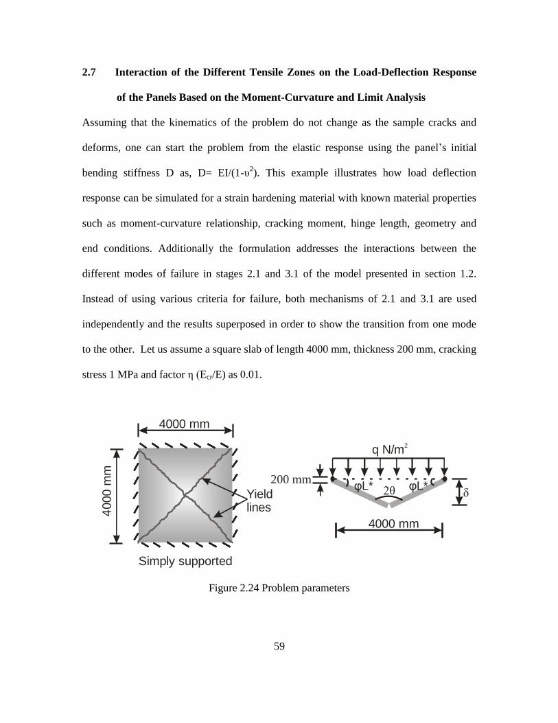
2.7 Interaction of the Different Tensile Zones on the Load-Deflection Response of
the Panels Based on the Moment-Curvature and Limit Analysis ......................................59
2.8 Post-Crack Analysis of ASTM C1550 Test results using the Proposed Yield
Line Load-Deflection Model .............................................................................................64
CHAPTER 3 - SHEAR PROPERTIES OF TEXTILE REINFORCED CONCRETE BY
MECHANICAL TESTS AND DIGITAL IMAGE CORRELATION ..............................67
3.1 Experimental Program.........................................................................................69
3.2 Shear Test Procedure and Instrumentation..........................................................70
3.3 Data Reduction Methods .....................................................................................73
3.3.1 Determination of Shear Force ....................................................................73
Page 6
vi
CHAPTER Page
3.3.2 Determination of Shear Angle ...................................................................75
3.3.3 Determination of Shear Strain ...................................................................77
3.1 Digital Image Correlation (DIC) method ............................................................78
3.1.1 Introduction and applications .....................................................................78
3.1.2 DIC discipline ............................................................................................81
3.2 Experimental Parameters.....................................................................................86
3.3 Analysis of Test Data ..........................................................................................89
3.4 Test Results .........................................................................................................89
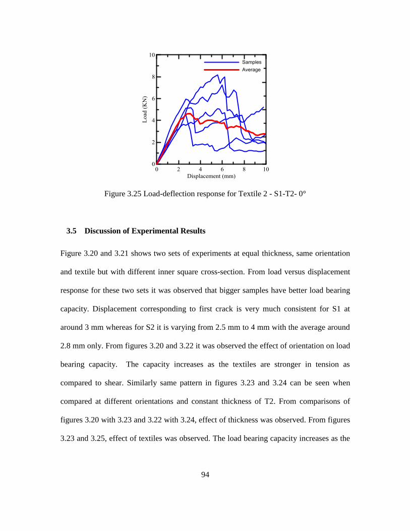
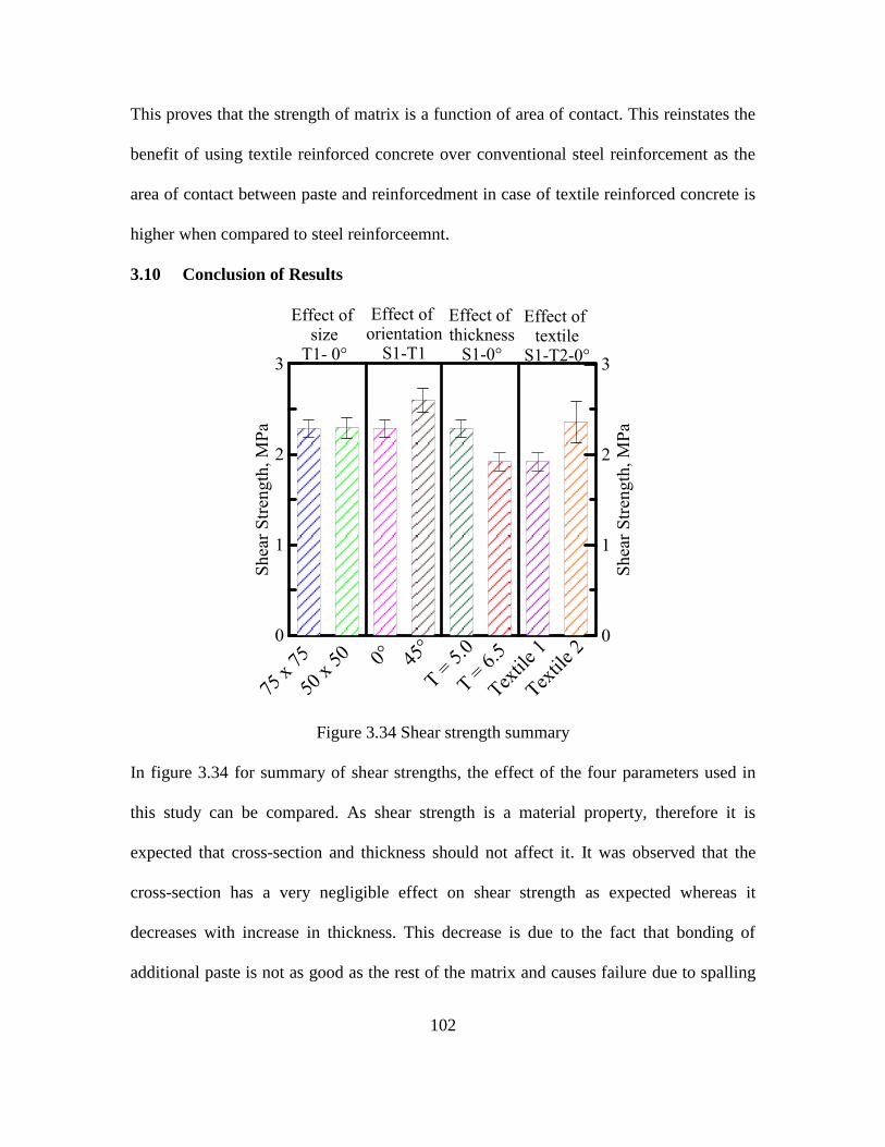
3.5 Discussion of Experimental Results ....................................................................94
3.6 Effect of Thickness..............................................................................................95
3.7 Effect of Orientation............................................................................................96
3.8 Effect of Planar Cross-section .............................................................................99
3.9 Effect of Textile Type .......................................................................................100
3.10 Conclusion of Results........................................................................................102
3.11 Digital Image Correlation Results .....................................................................104
3.12 Discussion of Digital Image Correlation results ...............................................108
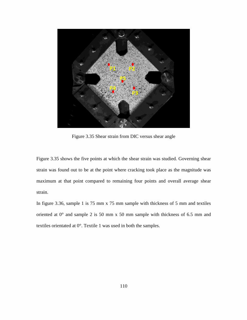
3.13 Relationship between Shear Angle and Shear Strain ........................................109
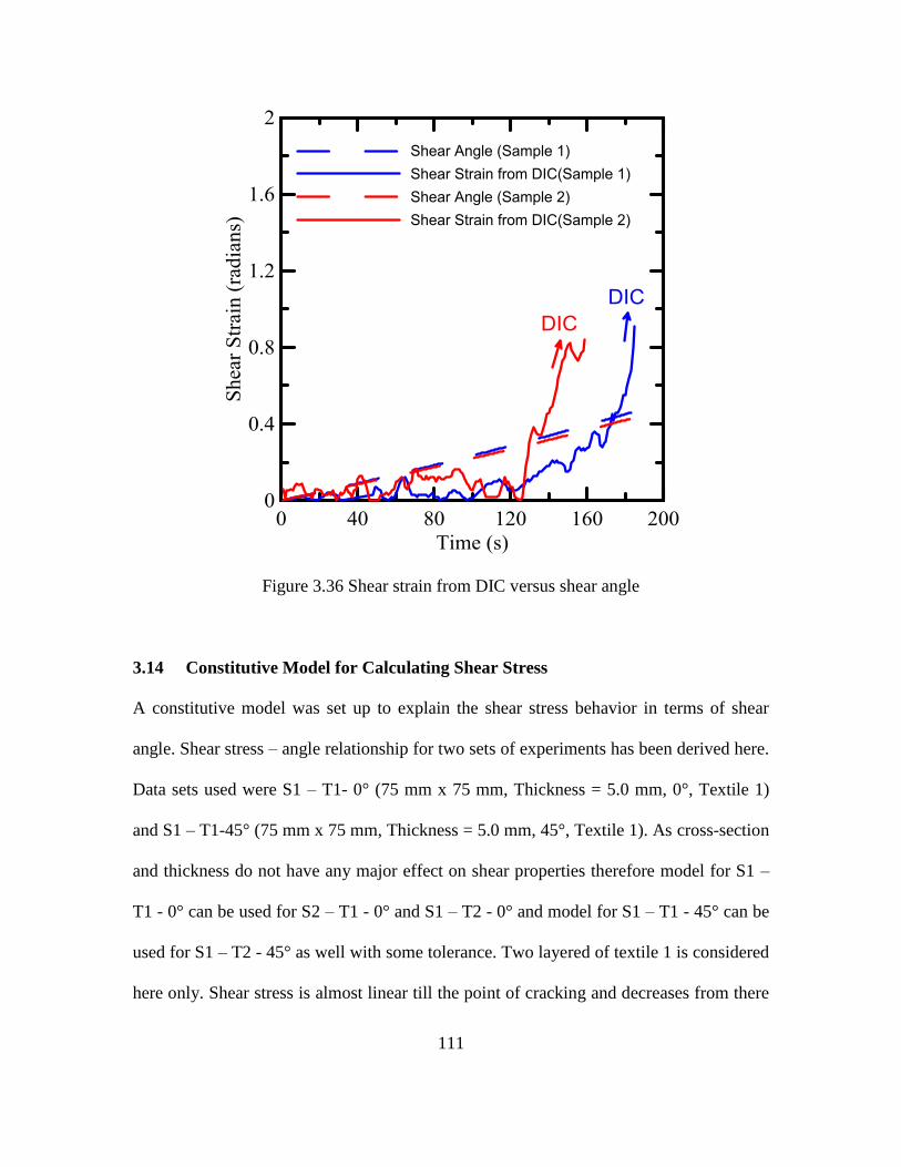
3.14 Constitutive Model for Calculating Shear Stress ..............................................111
3.1 Crack Pattern .....................................................................................................113
4. REFERENCES ..............................................................................................119
Page 7
vii
LIST OF FIGURES
Figure Page
1.1 Textile Reinforced Concrete ......................................................................................... 4
1.2 Full option material models for both strain-hardening and strain-softening material: (a)
tension model; and (b) compression model ........................................................................ 7
1.3 Strain and stress diagrams at the post crack stage (Ranges 2.1 and 3.1 - Table 1-2), (a)
strain distribution; and (b) stress distribution ..................................................................... 8
1.4 Effect of a) Depth of Neutral axis on the moment capacity of a section, and b) the
moment curvature response in the Range 2.1 ................................................................... 12
1.5 Schematics of pultrusion process ................................................................................ 15
1.6 Pultrusion setup with motors attached to the rollers ................................................... 16
1.7 Hand lay-up ................................................................................................................. 17
1.8 Hydraulic press ........................................................................................................... 17
2.1 Process for applied load-deflection derivation ........................................................... 19
2.2 Construction and applications of SHCC material slabs [] .......................................... 20
2.3 Simply supported square Panel with (a) yield lines and (b) loading and rotation
conditions through section A-A. ....................................................................................... 23
2.4 Applied load and yield line moment for a clamped square slab. ................................ 24
2.5 Two sides clamped and other two sides simply supported rectangular slab ............... 27
2.6 Applied load and yield line moment for a rectangular slab clamped on three sides and
free on fourth..................................................................................................................... 31
2.7 Principle of virtual work to determine the ultimate load carrying capacity of a round
panel test simply supported in its contour and subjected to center point load .................. 33
Page 8
viii
Figure Page
2.8 Hinge rotation mechanism (a) Steel fiber reinforced beam (BASF), (b) Rigid body
hinge rotation [16]............................................................................................................. 36
2.9 Load-deflection relationship for Square slab .............................................................. 37
2.10 Planes AED and EBC ............................................................................................... 37
2.11 Load-deflection relationship for Rectangular slab .................................................... 40
2.12 Planes KON and PLM .............................................................................................. 41
2.13 Planes KON and NOPM ........................................................................................... 42
2.14 Load-deflection for rectangular slab fixed from 3 sides and free from fourth ......... 44
2.15 Deflection-curvature relationship when yield lines are not at 45° ............................ 44
2.16 Load-deflection relationship for Circular slab .......................................................... 46
2.17 Flowchart for the derivation of applied load-deflection relationship for SHCC
materials ............................................................................................................................ 49
2.18 Different zones for slabs subjected to large displacements [21] ............................... 50
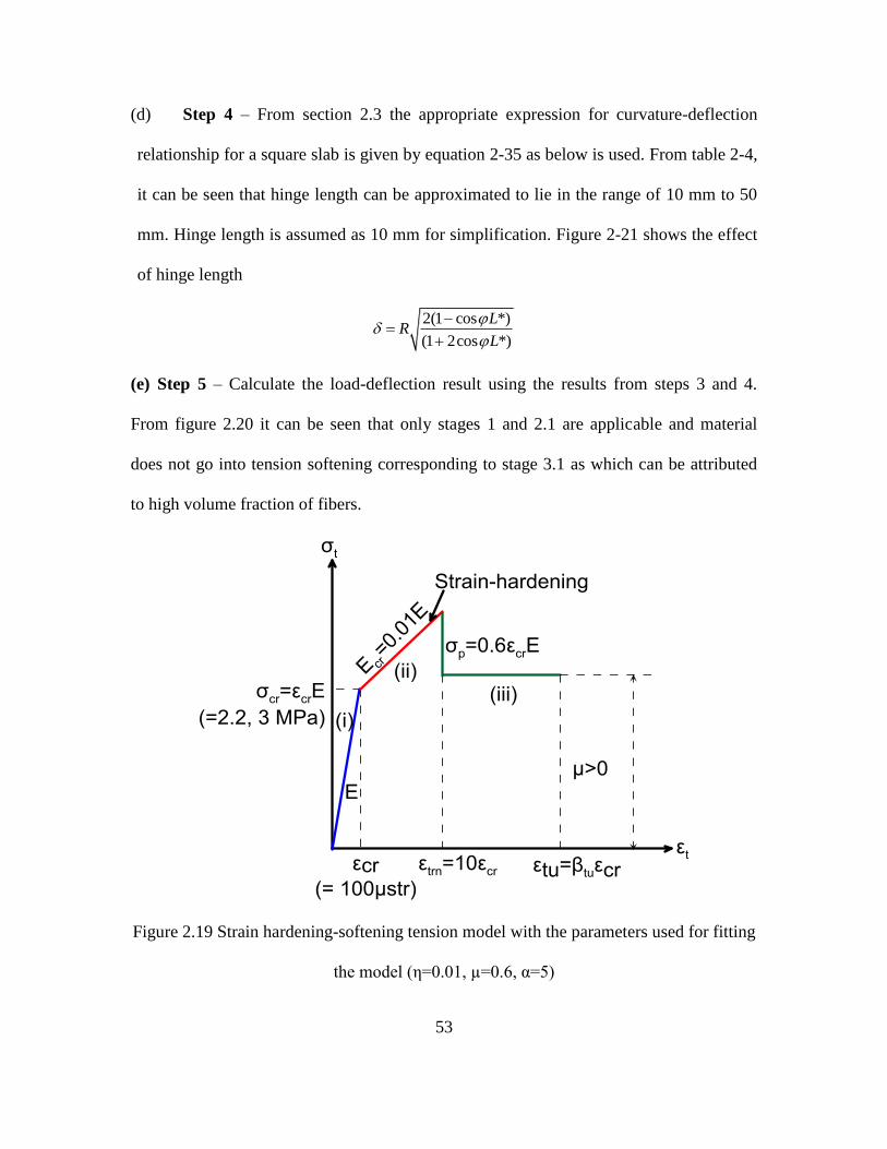
2.19 Strain hardening-softening tension model with the parameters used for fitting the
model (η=0.01, µ=0.6, α=5) .............................................................................................. 53
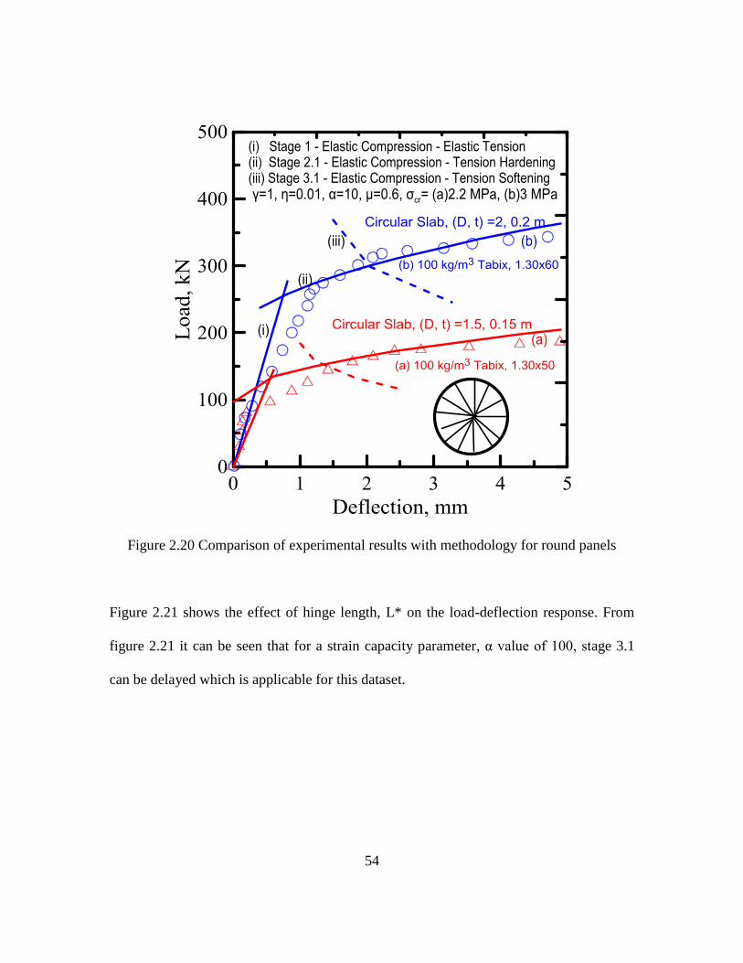
2.20 Comparison of experimental results with methodology for round panels ................ 54
2.21 Effect of hinge length on simulated results............................................................... 55
2.22 Experimental results for square slabs [23] ................................................................ 56
2.23 Comparison of experimental results with the methodology for square panels ......... 58
2.24 Problem parameters .................................................................................................. 59
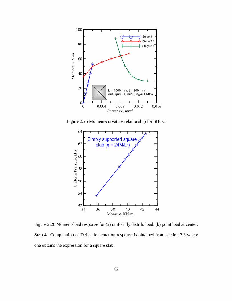
2.25 Moment-curvature relationship for SHCC................................................................ 62
Page 9
ix
Figure Page
2.26 Moment-load response for (a) uniformly distrib. load, (b) point load at center. ...... 62
2.27 Deflection-curvature relationship ............................................................................. 63
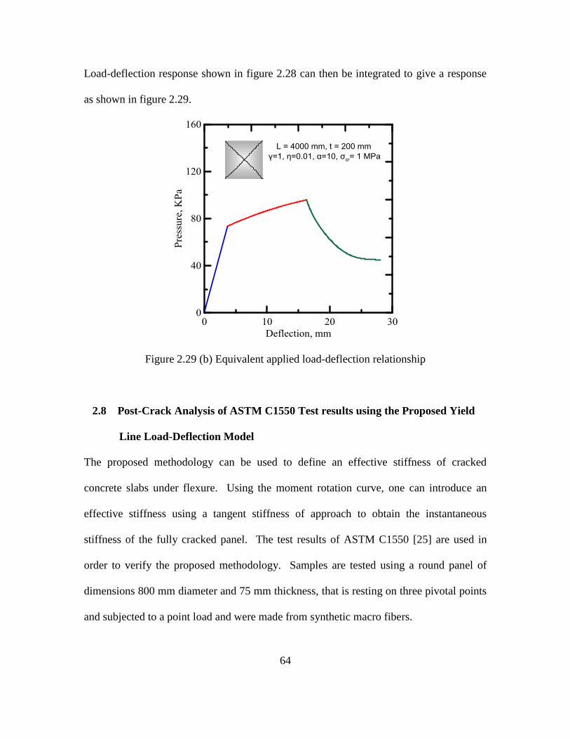
2.28 (a) Applied load-deflection relationship ................................................................... 63
2.29 (b) Equivalent applied load-deflection relationship .................................................. 64
2.30 Round panel tests (a) Test set up, (b) Comparison between the experimental data and
simplified model based on Johansen’s formula ................................................................ 66
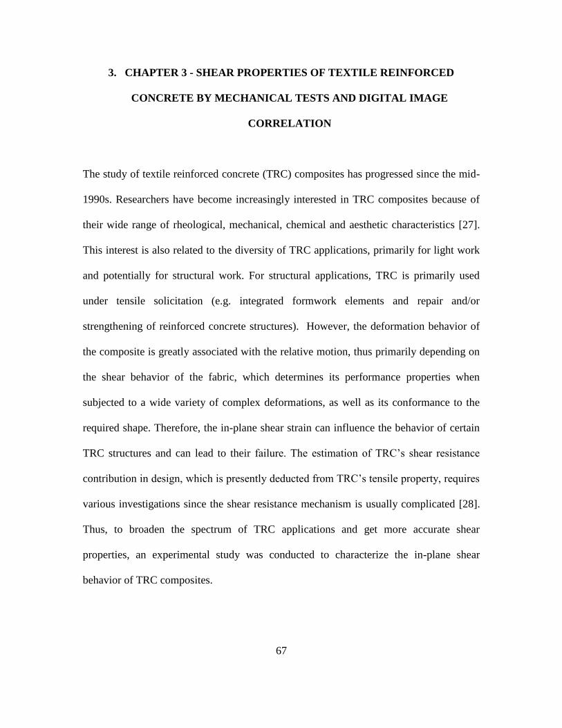
3.1 Methods of measuring shear force – (a) direct shear force measurement and (b)
picture frame test............................................................................................................... 68
3.2 Standard Hobart mixer ................................................................................................ 69
3.3 Test set-up ................................................................................................................... 71
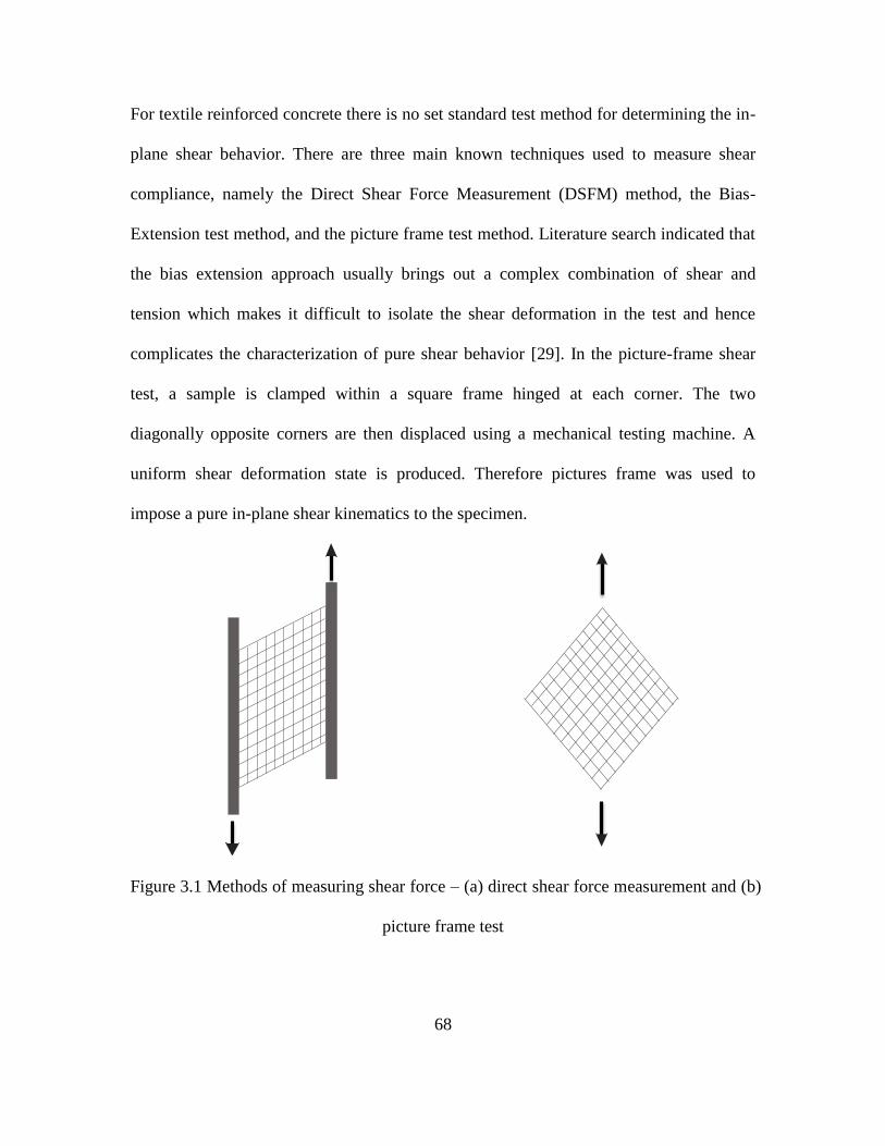
3.4 Schematics of test set-up ............................................................................................. 72
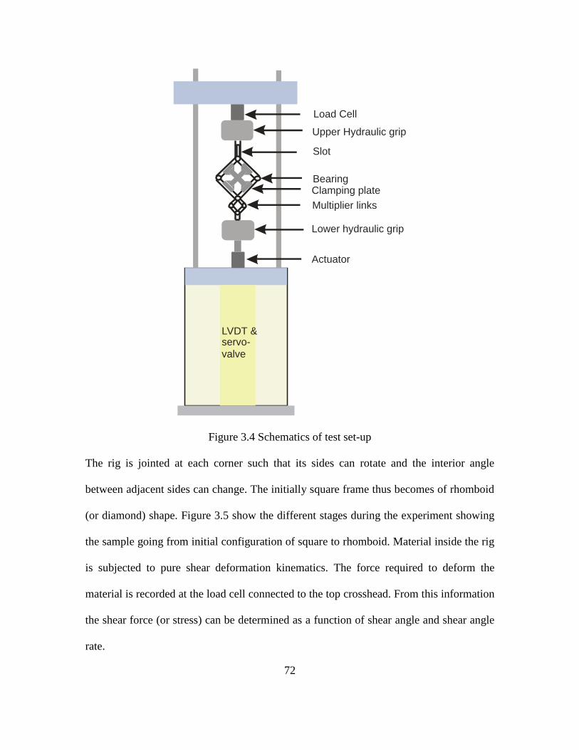
3.5 Different stages of experiment .................................................................................... 73
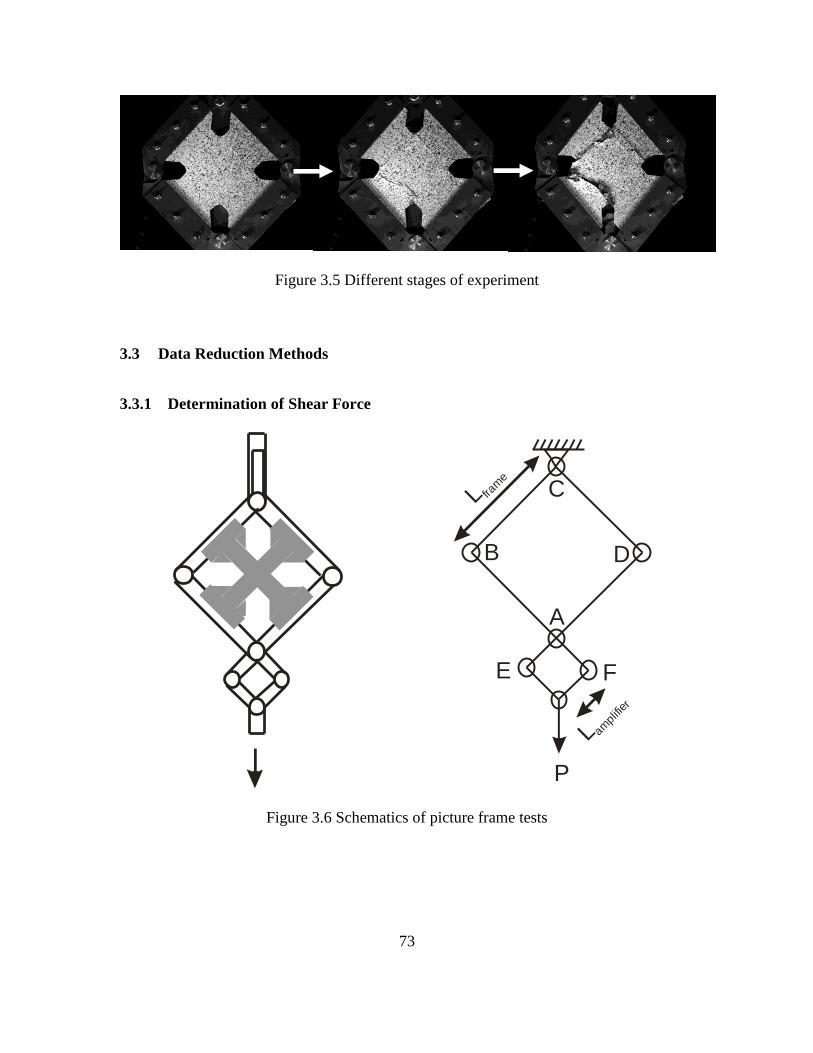
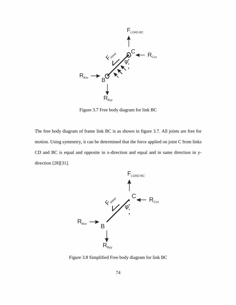
3.6 Schematics of picture frame tests ............................................................................... 73
3.7 Free body diagram for link BC ................................................................................... 74
3.8 Simplified Free body diagram for link BC ................................................................. 74
3.9 Initial configuration .................................................................................................... 76
3.10 Configuration after a displacement of D units .......................................................... 76
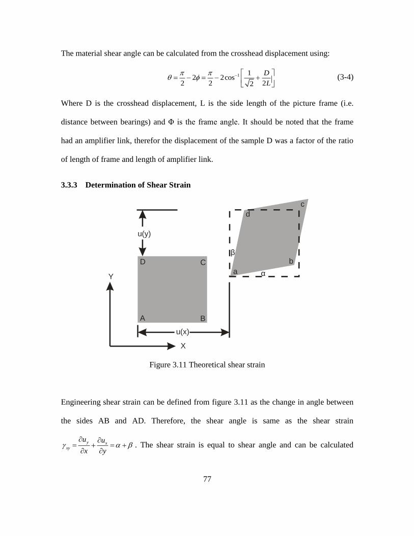
3.11 Theoretical shear strain ............................................................................................. 77
3.12 Setup of the 3D digital image correlation ................................................................. 80
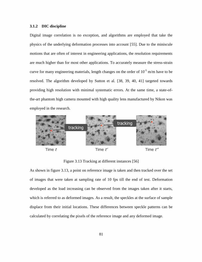
3.13 Tracking at different instances [] .............................................................................. 81
3.14 Mapping from original to deformed subset .............................................................. 82
3.15 Speckled samples ...................................................................................................... 82
Page 10
x
Figure Page
3.16 Terms involved in correlation [56] ........................................................................... 83
3.17 Correlation of a displaced surface [56] ..................................................................... 84
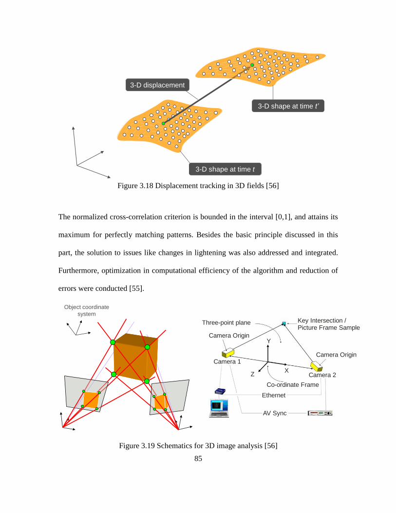
3.18 Displacement tracking in 3D fields [56] ................................................................... 85
3.19 Schematics for 3D image analysis [56] .................................................................... 85
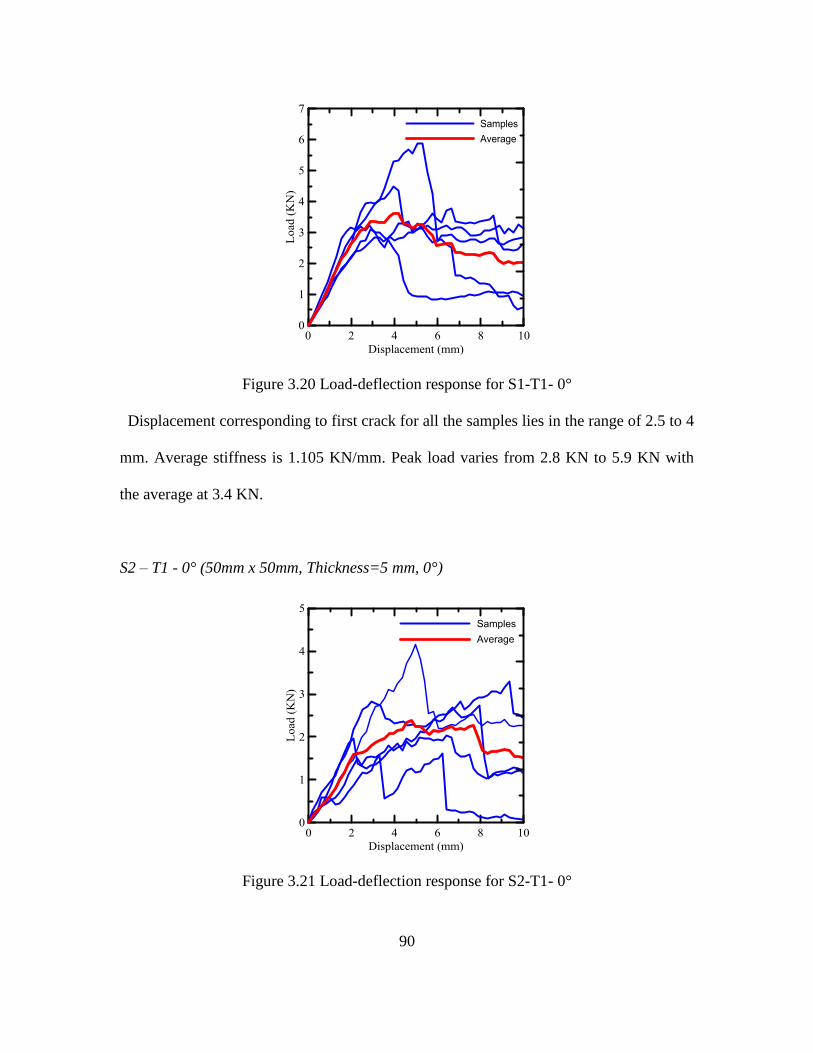
3.20 Load-deflection response for S1-T1- 0° ................................................................... 90
3.21 Load-deflection response for S2-T1- 0° ................................................................... 90
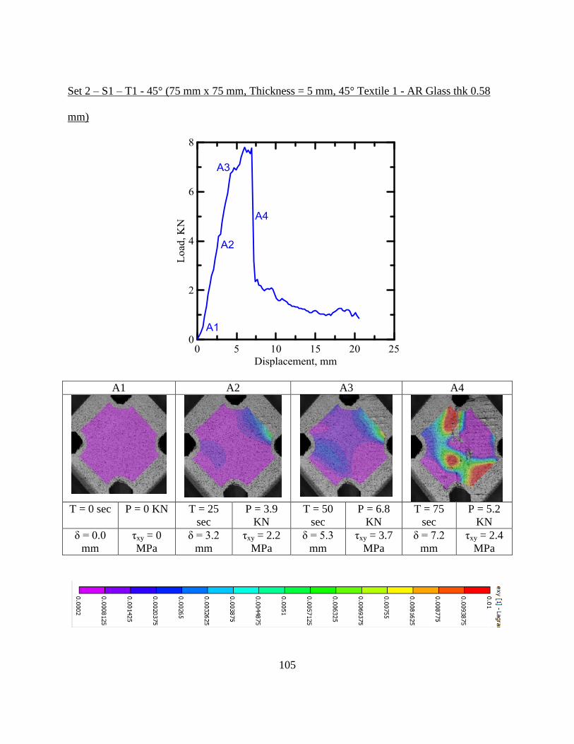
3.22 Load-deflection response for S1-T1- 45° ................................................................. 91
3.23 Load-deflection response for S1-T2- 0° ................................................................... 92
3.24 Load-deflection response for S1-T2- 45° ................................................................. 93
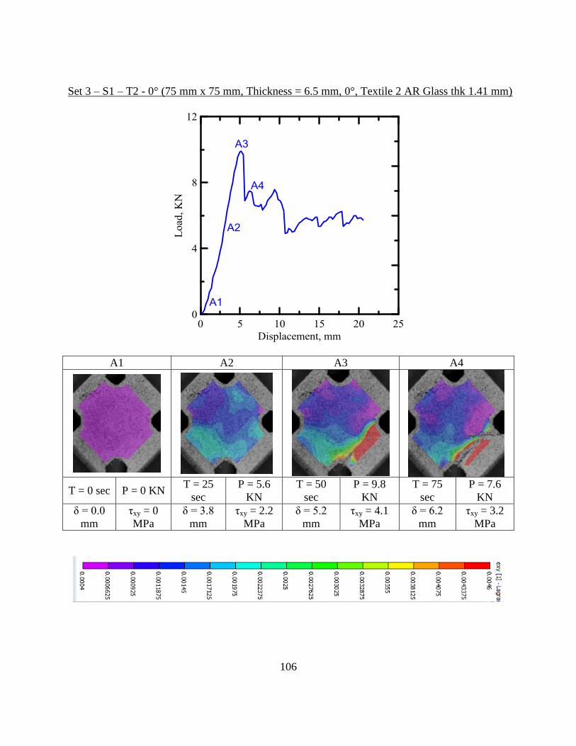
3.25 Load-deflection response for Textile 2 - S1-T2- 0° .................................................. 94
3.26 Shear stress versus shear angle response for comparison between the two
thicknesses - T1 (5.00 mm) and T2 (6.5 mm) for both the orientations ........................... 96
3.27 Orientations before and after cutting ........................................................................ 97
3.28 Shear stress versus shear angle response for comparison between the two
orientations- 0° and 45° for both the thicknesses ............................................................. 98
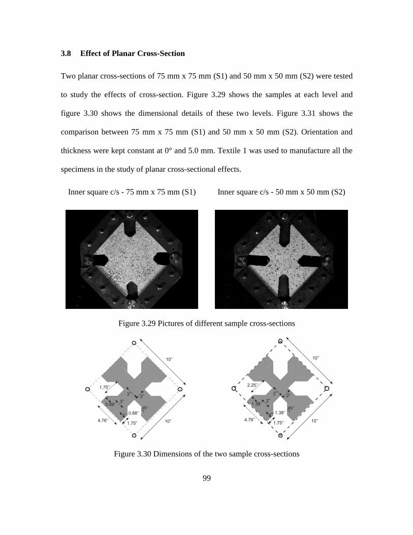
3.29 Pictures of different planar cross-section .................................................................. 99
3.30 Dimensions of the two planar cross-section ............................................................. 99
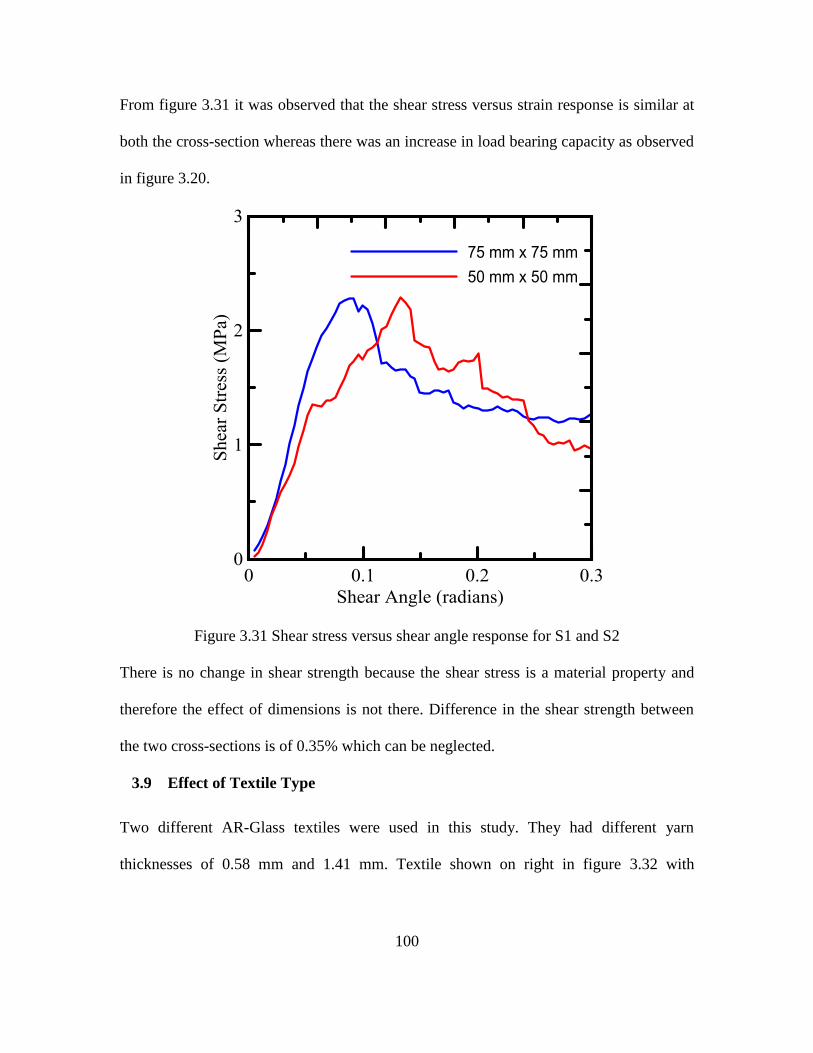
3.31 Shear stress versus shear angle response for S1 and S2 ......................................... 100
3.32 Two textiles used in this study ................................................................................ 101
3.33 Shear stress versus shear angle response for textile 1 vs textile 2 .......................... 101
3.34 Shear strength summary .......................................................................................... 102
3.35 Shear strain from DIC versus shear angle............................................................... 110
Page 11
xi
Figure Page
3.36 Shear strain from DIC versus shear angle............................................................... 111
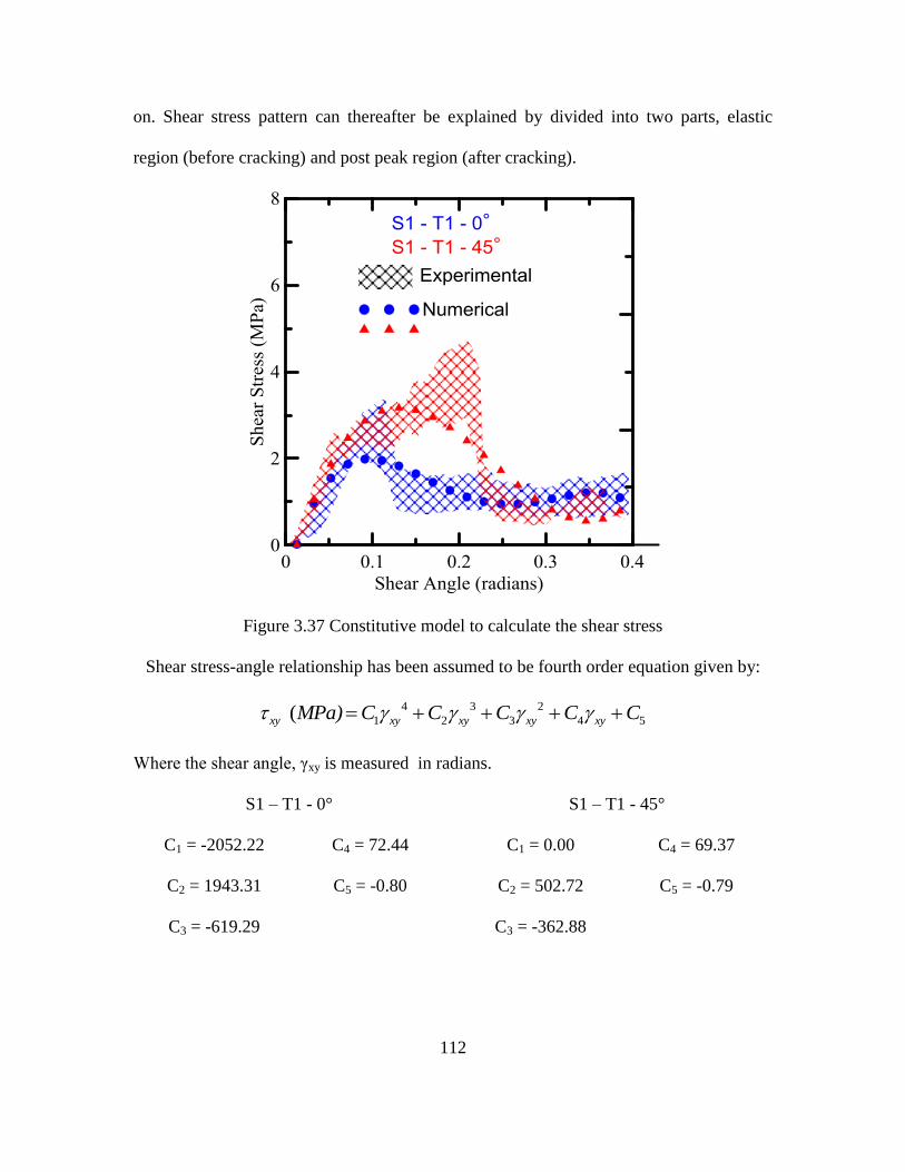
3.37 Constitutive model to calculate the shear stress ..................................................... 112
3.38 Different stage during the experiment .................................................................... 113
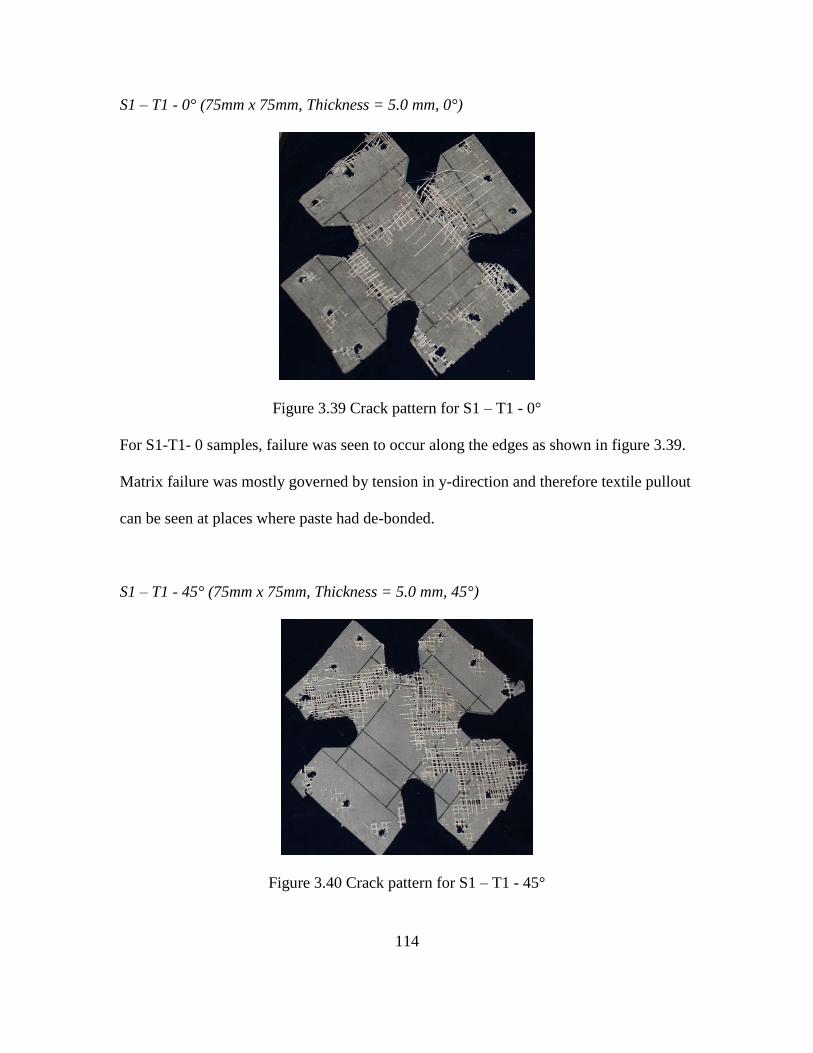
3.39 Crack pattern for S1 – T1 - 0° ................................................................................. 114
3.40 Crack pattern for S1 – T1 - 45° ............................................................................... 114
3.41 Crack pattern for S2 – T1 - 0° ................................................................................. 115
3.42 Crack pattern for S1 – T0 - 0° ................................................................................. 116
3.43 Crack pattern for S1 – T2 - 0° ................................................................................. 117
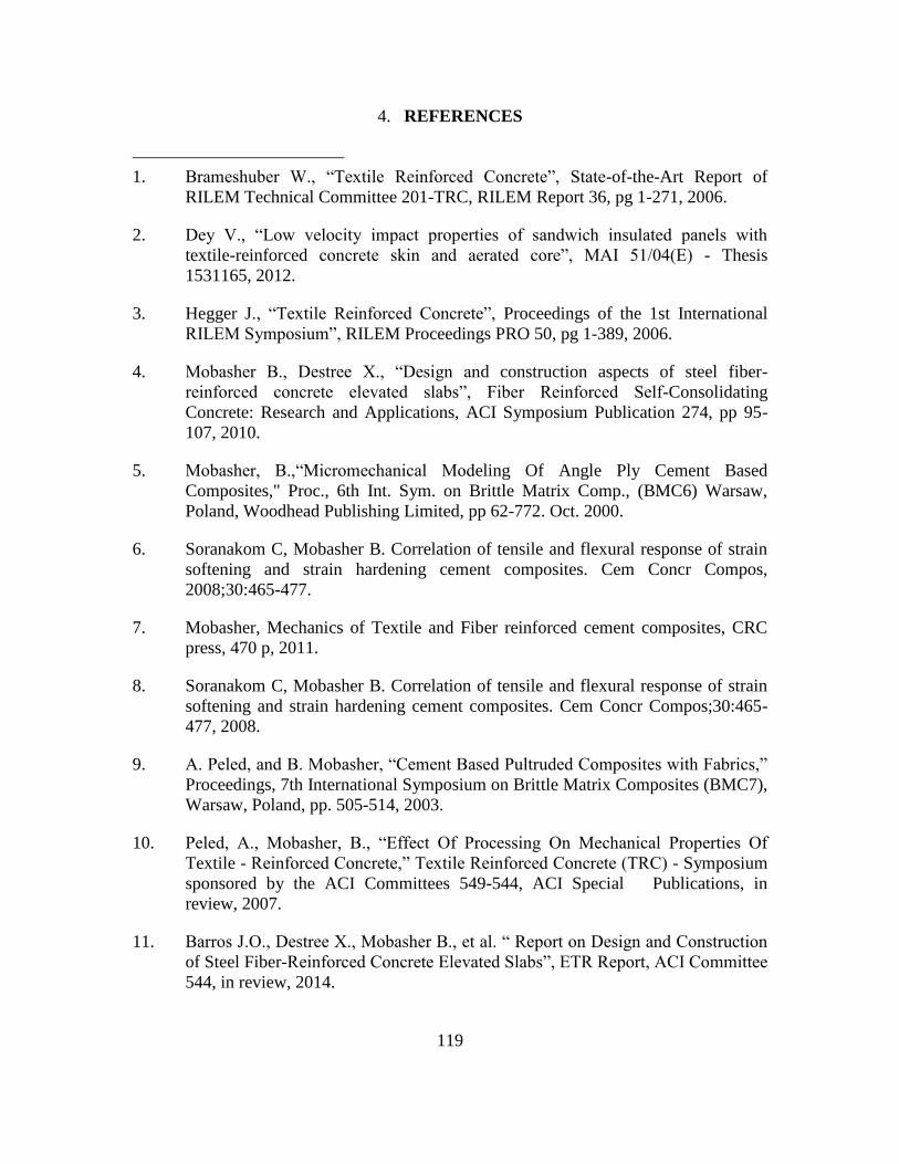
3.44 Crack pattern for Textile 2 – S1 – T2 - 0° .............................................................. 117
Page 12
xii
LIST OF TABLES
Tables Page
2-1 : Applied load – yield line moment relationship for Cases 1.1 to 1.3 ........................ 25
2-2 : Applied load – yield line moment relationship for Cases 2.1 to 2.4 ........................ 29
2-3 : Applied load – yield line moment relationship for Cases 3.1 and 3.2 ...................... 34
2-4 : Empirically derived hinge lengths ............................................................................ 36
3-1 : Mix design ................................................................................................................ 69
3-2 : Parameters tested and their levels........................................................................ 87
3-3 : Test combinations used in the experiment ............................................................... 88
3-4 : Summary of test results ............................................................................................ 95
Page 13
1
1. CHAPTER 1 - INTRODUCTION
1.1 Overview
The civil engineering profession recognizes the reality of limited natural
resources, the desire for sustainable development and the need for conservative
consumption of resources. On a global level, there is a great demand of building material
to sustain the exponential growth of infrastructure [1]. Concrete being one of the most
consumed building materials; a lot of research is going on in increasing its durability,
designing light weight structural members, developing building systems with low cement
and utilizing renewable energy resources. Lowering the cost of building materials is also
one of the key aspects of sustainable infrastructure especially in the developing nations.
Plain concrete has always been known to be a brittle material with weak tension
capacities. Fabric based cement composites aid in improving tensile strength and
stiffness along with introduction of ductility in the infrastructure systems and come under
the broad category of strain hardening or strain softening cement composites [ 2 ].
Therefore strain hardening cement composites (SHCC) such as textile reinforced concrete
have become integral research topic. Applications of SHCC material has been further
extended to panels and shear elements due to their improved performance taking into
account serviceability and sustainability. This study is majorly based on evaluating the
performance of strain hardening cement composites for improving durability and
ductility.
Page 14
2
1.1.1 Strain Hardening Cement Composite
Strain hardening materials are well suited for applications that eliminate conventional
reinforcement or for the structures in seismic regions where high ductility is desired. In
addition, these materials offer fatigue and impact resistance and are attractive for use in
industrial structures, highways, bridges, earthquake, hurricane, and high wind loading
conditions. The design and implementation of these systems requires one to acknowledge
and use the strain-hardening response that is attributed to multiple cracking. Propagation
of initial crack in strain hardening composites is resisted by bridging mechanism. Since a
substantial amount of energy is required to further extend existing cracks, secondary
cracks form. Single crack localization is therefore shifted to multiple distributed cracking
mechanisms, leading to macroscopic pseudo-strain hardening behaviors. The dominant
toughening mechanisms in these systems are attributed to matrix cracking, ply
delamination, and crack deflection mechanisms as studied by means of fluorescent
microscopy and scanning electron microscopy.
1.1.2 Textile Reinforced Concrete as a Strain Hardening Cement Composite
Reinforcement is commonly combined with plain concrete to enhance its tensile strength
[3]. There are various types of materials and forms used for reinforcing, but the most
common is round steel bars with ribs. Reinforced concrete structures with steel are
vulnerable to corrosion attack if the protective medium provided by concrete is
weakened. In an attempt to improve the durability, other reinforcement options such as
stainless steel bars, epoxy-coated steel bars, fiber-reinforced polymer (FRP) bars, steel
welded-wire fabric, and fibers (steel and synthetic) have been explored. A recent
Page 15
3
innovative attempt to improve the sustainability of reinforced concrete is the
development of Textile Reinforced Concrete (TRC). It was discovered that TRC can be
utilized to build slender, lightweight, modular and freeform structures and eliminate the
risk of corrosion. TRC provides high strength in compression and tension and is proven
to be a suitable option for the strengthening of existing structures. This composite
material is fabricated using a fine-grained concrete matrix reinforced by multi-axial
textile fabrics. The underlying concept of TRC is based on a combination of traditionally
used reinforcement bars and FRC, wherein the shortcomings of both reinforcement
methods, namely durability and design control, are overcome. TRC is explored as a
sustainable solution because its design minimizes the use of binder material such as
concrete, which when made of Portland cement is one of the most pollutant and energy
consuming building materials used in the construction industry. Focusing on the
reduction and replacement of energy-intensive materials like Portland cement not only
helps to reduce the extraction of natural resources but also to reduce the high energy
demands of the production process. The use of textile reinforcement made from non-
corrosive materials, such as carbon and glass can reduce the required concrete material by
up to 85%. Typical mechanical properties of the textile reinforced concrete measured
using uniaxial tensile, flexural, and shear tests indicate that the tensile strength of around
25 MPa, and strain capacity of 1-8% [4]. The fracture toughness as compared to the
conventional FRC materials is increased by as much as two orders of magnitude. For
Textile Reinforced Concrete applications, bi- or multi-axial 2D and 3D textile meshes
can be used as reinforcement. For a simple bi-axial case, the mesh comprises two groups
of textile fiber yarns (threads), warp (0°) and weft (90°), interwoven perpendicularly to
Page 16
4
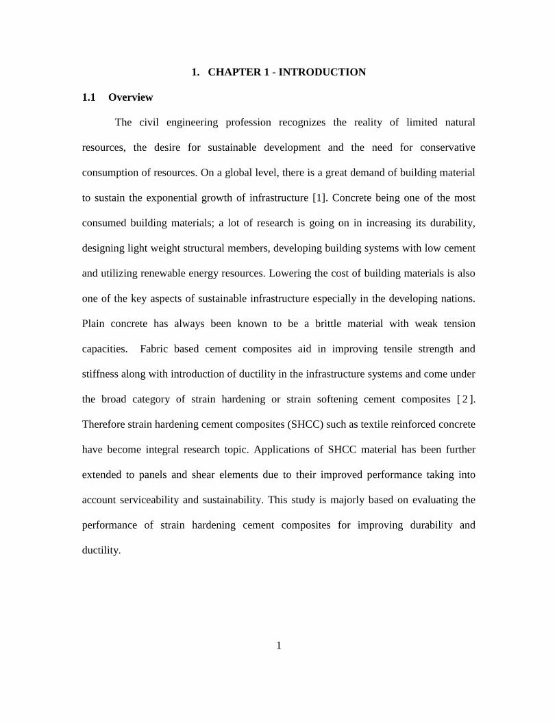
each other. Yarns are composed of multiple single fibers of continuous length, also
designed as filaments; grouping of continuous fibers is primarily done to obtain the
desired thickness of yarn. Fabrication methods related to textile meshes are abundant and
can be tailored to the needs of nearly any given application. In the case of TRC, an open-
grid structure and displacement stability are favored in order to allow for adequate
penetration of a cementitious matrix, whilst ensuring a relatively constant woven mesh
structure in composite form.
Figure 1.1 Textile Reinforced Concrete
1.1.3 Materials
The choice of fiber material for use in TRC is based on various factors such as material
properties, corrosion and temperature resistance, bond quality, demand/production cost
and even environmental impact. In terms of mechanical behavior, tensile strength,
breaking elongation and modulus of elasticity superior to those related to the
cementitious matrix is essential. The reinforcement ratio and placement of the textile
reinforcement will also have a great impact on the composite behavior of a TRC member.
Fiber materials which have generally been used and explored in TRC include, but are not
limited to: alkali-resistant glass (AR-glass), carbon, basalt, aramid, polyvinyl-alcohol
(PVA) with polyvinyl chloride (PVC) coating. In this thesis, only AR-glass has been
explored, as it is the most readily available and applied material.
Page 17
5
Glass fibers are chemical fibers derived from inorganic non-metallic raw materials. The
raw materials needed to produce AR-glass are primarily silica sand (SiO2) and the
addition of zircon (ZrO2) to provide superior alkali resistance, which are proportioned
through a batching process. These raw materials undergo a melting process between 1250
to 1350°C, wherein molten glass is yielded. Fiberization of the molten glass takes places
afterwards, meaning that fibers are produced through a wet-spinning process. The glass
fiber filaments are then sized to primarily protect them against damage during packaging
and finishing. Coating is often applied during sizing to obtain a specified surface wetting
and bonding of the filaments. AR Glass used in this study had a tensile strength in range
of 1270 – 2450 MPa and modulus of elasticity of 78 MPa.
1.2 Simplified Strain-hardening Cement composites (SHCC) Model
In strain hardening cement composites fabric systems are used with an efficient interface
bond which enhances load transfer across a matrix crack. If fiber volume fraction is
higher than a critical level, the entire load can be transferred through the fiber, and
subsequent cracking of the matrix can take place leading to distributed cracking and
significant strain capacity. Effect of distributed cracking on the stiffness degradation of
the composite under tensile loading is then used to represent the reduction in the modulus
and stiffness of the sample in the tension, allowing for the strain capacity to be included
in the design procedure. Using damage function modeling, the post crack stiffness is
calibrated by predicting the ultimate strength of composites under tensile and
compressive loading and the results are utilized to correlate the distributed cracking in
strain hardening composites with various fiber types and contents under tension [5].
Page 18
6
Application of strain compatibility analysis to a new constitutive model requires layer
discretization, iterative solution for neutral axis, and numerical integration to determine
moment and curvature at each strain increment. Since the compression and tension
response of various cement composites listed above are relatively close, closed-form
solution of moment-curvature diagram, derived for a generic material can be used to
predict flexural behavior of homogenized fiber/fabric reinforcement. Closed form
solutions of a moment-curvature relationship can also be directly implemented in a
structural analysis code, and/or spreadsheets.
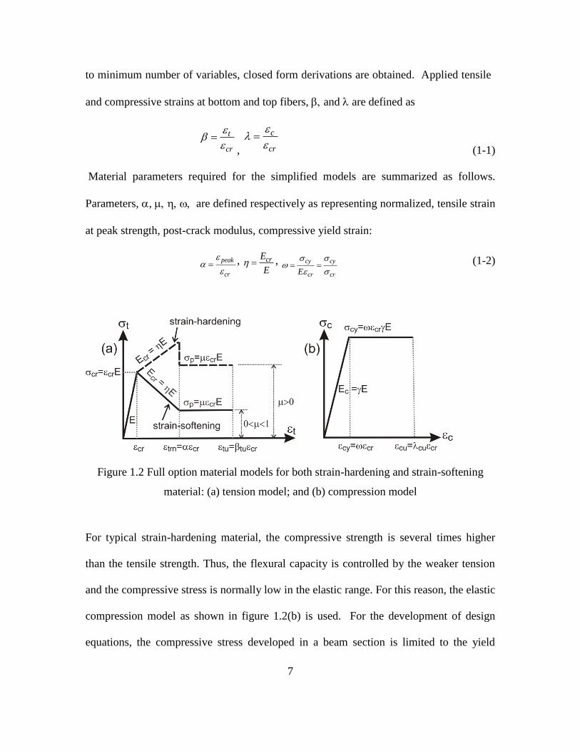
A general strain hardening tensile, and an elastic perfectly plastic compression model as
derived by Soranakom and Mobasher [6] [7] [8] and shown in figure 1.2 is used.
Tensile response is defined by tensile stiffness, E, first crack tensile strain, cr, Cracking
tensile strength, cr =Ecr, ultimate tensile capacity, peak, and post crack modulus, Ecr.
The softening range is shown as a constant stress level, Ecr. The compression
response is defined by the compressive strength, cy defined as Ecr. In order to
simplify material characteristics of strain-hardening material, and yet obtain closed form
design equation generation several assumptions are made. Equations can furthermore be
simplified to idealized tri-linear tension and elastic compression models as shown in
figure 1.2 (a) and (b) by ignoring the post-peak ranges in both tension and compression.
In order to reduce the complexity of material response to the useable range, one has to
disregard the post-peak tensile response and plasticity in the compression region. It has
been shown that the difference in compressive and tensile modulus has negligible effect
to the ultimate moment capacity. By defining all parameters as normalized with respect
Page 19
7
to minimum number of variables, closed form derivations are obtained. Applied tensile
and compressive strains at bottom and top fibers, and are defined as
t
cr
,
c
cr
(1-1)
Material parameters required for the simplified models are summarized as follows.
Parameters, , are defined respectively as representing normalized, tensile strain
at peak strength, post-crack modulus, compressive yield strain:
peak
cr
, crE
E , cy cy
cr crE
(1-2)
Figure 1.2 Full option material models for both strain-hardening and strain-softening
material: (a) tension model; and (b) compression model
For typical strain-hardening material, the compressive strength is several times higher
than the tensile strength. Thus, the flexural capacity is controlled by the weaker tension
and the compressive stress is normally low in the elastic range. For this reason, the elastic
compression model as shown in figure 1.2(b) is used. For the development of design
equations, the compressive stress developed in a beam section is limited to the yield
Page 20
8
compressive stress cy = 0.85fc’ at compressive yield strain cy, where fc’ is the uniaxial
compressive strength.
ctop cr=
tbot cr=
1
1hc1
ht1
kd
d1
1yc1
yt1
Fc1
yt2ft1
fc1
2 ht2
cr
Ft22
ft2
Ft1
(2.1)
ctop cr=
tbot cr=
1
1hc1
ht1
kd
d1
1yc1
yt1
Fc1
yt2ft1
fc1
2 ht2
cr
Ft22ft2
Ft1
(3.1)
3 ht3 3 Ft3
yt3
ft3
trn
(a) (b)
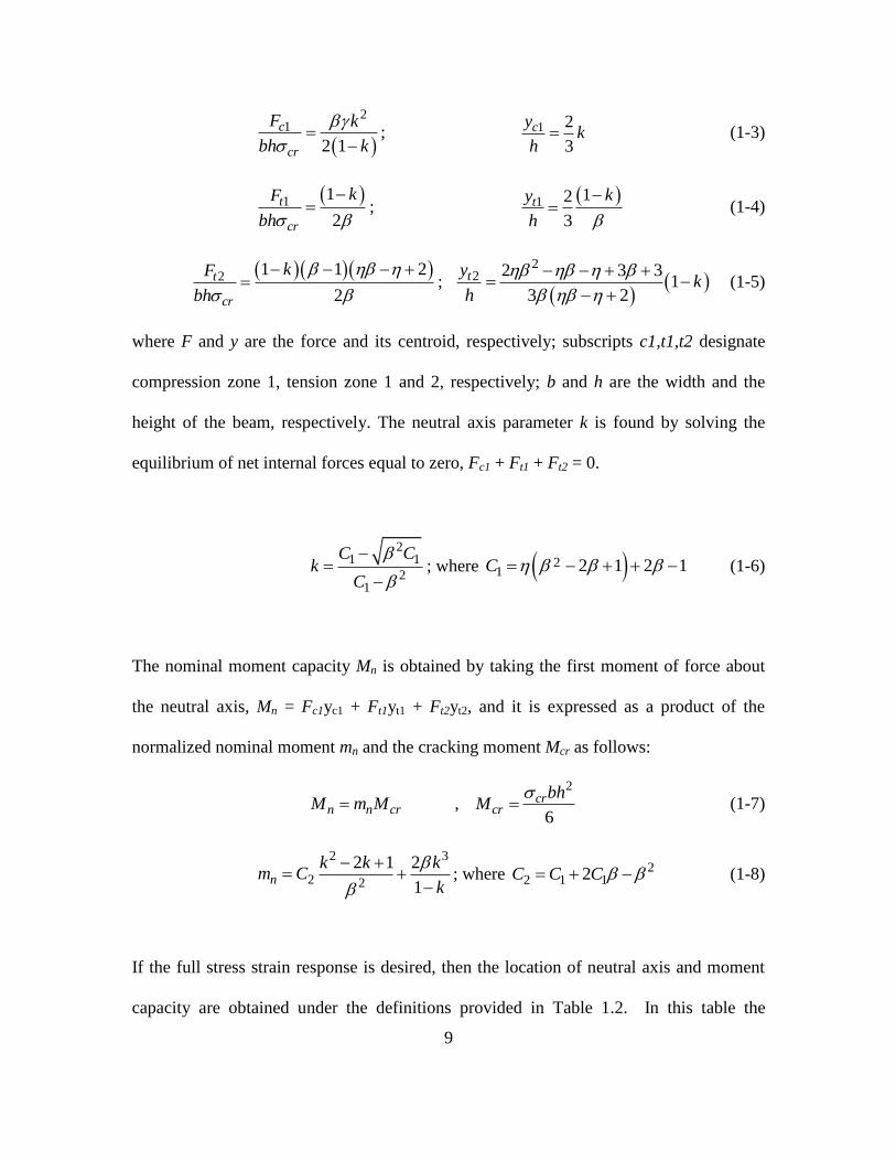
Figure 1.3 Strain and stress diagrams at the post crack stage (Ranges 2.1 and 3.1 - Table
1-2), (a) strain distribution; and (b) stress distribution
1.2.1. Derivation of Moment-Curvature Capacity
Moment capacity of a beam section according to the imposed tensile strain at the bottom
fiber (t = cr) can be derived based on the assumed linear strain distribution as shown in
Fig. 2(a). By using material models described in figure 1.2 (a) and (b), the corresponding
stress diagram is obtained as shown in figure 1.3 (b) in which the stress distribution is
subdivided into a compression zone 1, tension zone 1 and 2. Force components and their
centroidal distance to the neutral axis in each zone can be expressed as:
Page 21
9
21
2 1
c
cr
F k
bh k
; 1 2
3
cyk
h (1-3)
1 1
2
t
cr
kF
bh
;
1 12
3
t ky
h
(1-4)
2 1 1 2
2
t
cr
kF
bh
;
22 2 3 3
13 2
tyk
h
(1-5)
where F and y are the force and its centroid, respectively; subscripts c1,t1,t2 designate
compression zone 1, tension zone 1 and 2, respectively; b and h are the width and the
height of the beam, respectively. The neutral axis parameter k is found by solving the
equilibrium of net internal forces equal to zero, Fc1 + Ft1 + Ft2 = 0.
21 1
21
C Ck
C
; where 2
1 2 1 2 1C (1-6)
The nominal moment capacity Mn is obtained by taking the first moment of force about
the neutral axis, Mn = Fc1yc1 + Ft1yt1 + Ft2yt2, and it is expressed as a product of the
normalized nominal moment mn and the cracking moment Mcr as follows:
2
,6
crn n cr cr
bhM m M M
(1-7)
2 3
2 2
2 1 2
1n
k k km C
k
; where 2
2 1 12C C C (1-8)
If the full stress strain response is desired, then the location of neutral axis and moment
capacity are obtained under the definitions provided in Table 1.2. In this table the
Page 22
10
derivations of all potential combinations for the interaction of tensile and compressive
response are presented. Note that depending on the relationship among material
parameters, any of the zones 2.1, and 2.2, or 3.1, and 3.2 are potentially possible.
Analysis of these equations indicates that the contribution of fibers is mostly apparent in
the post cracking tensile region, where the response continues to increase after cracking
[figure 1.2 (a)]. The post-crack modulus Ecr is relatively flat with values of = 0.00-0.4
for a majority of cement composites. The tensile strain at peak strength peak is relatively
large compared to the cracking tensile strain cr and may be as high as = 100 for
polymeric based fiber systems. These unique characteristics cause the flexural strength
to continue to increase after cracking. Since typical strain-hardening material do not have
significant post-peak tensile strength, the flexural strength drops after passing the tensile
strain at peak strength. Furthermore the effect of post crack tensile response parameter
can be ignored for a simplified analysis. In the most simplistic way, one needs to
determine two parameters in terms of post crack stiffness and post crack ultimate
strain capacity to estimate the maximum moment capacity for the design purposes.
According to bilinear tension and elastic compression models shown in figure 1.2 (a) and
(b), the maximum moment capacity is obtained when the normalized tensile strain at the
bottom fiber ( = t/cr) reaches the tensile strain at peak strength ( = peak/cr). However,
the simplified equations 1-6 to 1-8 for moment capacity are applicable for the
compressive stress in elastic region only. The elastic condition must be checked by
computing the normalized compressive strain developed at the top fiber and compare it
Page 23
11
to the normalized yield compressive strain . The general solutions for all the cases are
presented in table 1.2. Using the strain diagram in Fig. 1.3 (a), the relationship between
the top compressive strain and bottom tensile strain as follow:
1
c t
kh k h
(1-9)
By substituting c = cr and t = cr in equation 1-9, then defining the maximum
compressive strain to the yield compressive strain cy = cr , equation 1-9 is expressed in
normalized form:
1
k
k
(1-10)
The case represented by case 2.1 of the table 1.2, where the tensile behavior is in elastic-
plastic while the compressive behavior is still elastic is studied in this section. Equations
for other cases can also be developed. The general solution presented in table 1.1 can be
simplified as follows. The location of neutral axis represented as a function of applied
tensile strain is represented as:
2A ( 1 2 )k 2A
A1 (1-11)
This equation can be easily simplified by assuming equal tension and compression
stiffness ( For an elastic perfectly plastic tension material ( equation 1-11
reduces to:
2 1
2 1
k (1-12)
Page 24
12
Figure 1.4 Effect of a) Depth of Neutral axis on the moment capacity of a section, and b)
the moment curvature response in the Range 2.1
Table 1.1 presents the case of (, for different values of post-crack stiffness .5,
0.2, 0.1, 0.05, 0.01, and 0.001. Note that the neutral axis is a function and can be used
in calculation of the moment, or the moment-curvature relationship. These general
responses are shown in Figures 1.4a and 1.4b and show that with an increase in applied
tensile strain, the neutral axis compression zone decreases; however this decrease is a
function of post crack tensile stiffness factor. The moment curvature relationship in this
range in ascending, however, its rate is a function of the post crack tensile stiffness. The
parameter based fit equations in the third and fourth column are obtained by curve fitting
the simulated response from the closed form derivations and are applicable within 1%
accuracy of the closed form results. Using these equations, one can generate the moment
0 10 20 30 40 50
Normalized Curvature, '
0
2
4
6
8
10N
orm
aliz
ed M
om
ent, M
'
=0.05
=0.10
=0.20
=0.00
=0.01
0 10 20 30 40 50
Normalized Curvature, '
0
0.1
0.2
0.3
0.4
0.5
No
rmaliz
ed
Ne
utr
al A
xis
=0.05
=0.10
=0.20
=0.00
=0.01
Page 25
13
capacity and moment-curvature response for any cross section using basic tensile
material parameters in the 2.1 range as defined.
A, (
Ak
A
)
)'(M k )'(M
0.5 20.5( 1- 2 ) 2 -1 1 60.773 0.108 10 x k 0.507 0.686
0.2 20.2( 1- 2 ) 2 -1 2 60.654 0.516 10 x k 1.105 0.383
0.1 20.1( 1- 2 ) 2 -1 2 61.276 0.289 10 x k 1.461 .234
0.05 20.05( 1- 2 ) 2 -1 2 61.645 .1632 10 x k 1.720 .1401
0.01 20.01( 1- 2 ) 2 -1 10.852 0.456 k 1.342 0.371
0.0001 20.0001( 1- 2 ) 2 -1 3.177 3.068 k 3.021 2.047 /
Table 1-1: Location of Neutral axis, moment, and moment-curvature response of a strain
hardening composite material with = 1, = 0.0001- 0.5.
Page 26
14
Stage k m = M/Mcr =Φ/ Φcr
1 0 <
< 1 1
1 for =1
2
1 for 1
1
k
3 21 1 1
11
2 1 3 3 1
1
k k km
k
1
1
'2 1 k
2.1 1 <
< 0 <
<
221 21
21 221
D Dk
D
221 2 1 2 1D
3 3 221 21 21 21 21 21 21
2121
2 3 3'
1
C k C k C k CM
k
3 2 2
21 2
(2 3 1) 3 1C
2121
'2 1 k
2.2 1 <
< <
< cu
2222
22 2
Dk
D
222 21D D
2 222 22 22 22 22 22' 3 2M C k C k C
3
22 21 2C C
2222
'2 1 k
3.1 <
< tu
0 <
<
231 31
31 231
D Dk
D
231 2 1 2 2 1D
3 3 231 31 31 31 31 31 31
3131
2 3 3'
1
C k C k C k CM
k
3 2 2 2 2
31 2
(2 3 1) 3 3 1C
3131
'2 1 k
3.2 <
< tu
<
< cu
3232
32 2
Dk
D
232 31D D
2 232 32 32 32 32 32' 3 2M C k C k C
3
32 31 2C C
3232
'2 1 k
Table 1-2 : Neutral axis parameter k, normalized moment m and normalized curvature for each
stage of normalized tensile strain at bottom fiber (
Page 27
15
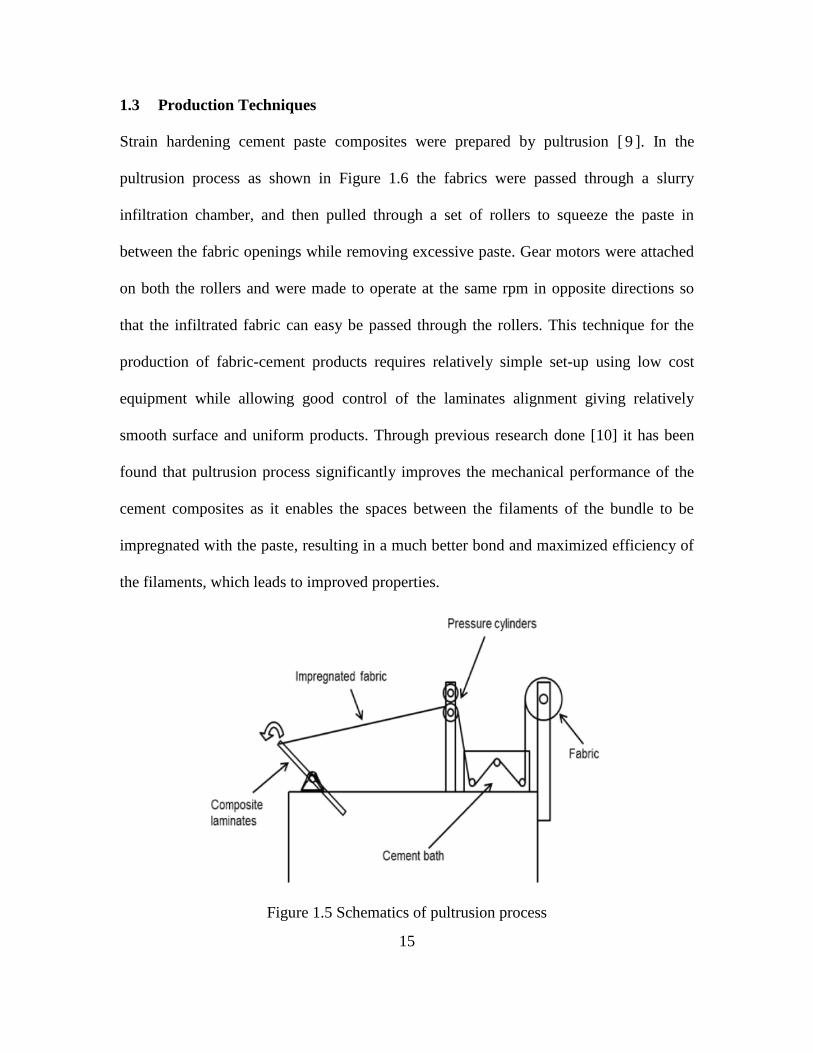
1.3 Production Techniques
Strain hardening cement paste composites were prepared by pultrusion [ 9 ]. In the
pultrusion process as shown in Figure 1.6 the fabrics were passed through a slurry
infiltration chamber, and then pulled through a set of rollers to squeeze the paste in
between the fabric openings while removing excessive paste. Gear motors were attached
on both the rollers and were made to operate at the same rpm in opposite directions so
that the infiltrated fabric can easy be passed through the rollers. This technique for the
production of fabric-cement products requires relatively simple set-up using low cost
equipment while allowing good control of the laminates alignment giving relatively
smooth surface and uniform products. Through previous research done [10] it has been
found that pultrusion process significantly improves the mechanical performance of the
cement composites as it enables the spaces between the filaments of the bundle to be
impregnated with the paste, resulting in a much better bond and maximized efficiency of
the filaments, which leads to improved properties.
Figure 1.5 Schematics of pultrusion process
Page 28
16
Figure 1.6 Pultrusion setup with motors attached to the rollers
Pultruded samples were very thin and not feasible for testing. Therefore, after the fabrics
were passed through the rollers, additional cement paste was applied on each surface
using the traditional hand lay-up technique. This was done to improve the thickness of
the final composite and make it more workable. Consistent amount of cement paste (by
weight) was added on each layer depending on the final thickness required. For the
samples with final thickness of 5 mm, 350 grams of cement paste was added on each
layer and for 6.5 mm thick samples, 450 grams of cement paste was applied on each layer.
After forming the samples, pressure was applied on top of the fabric-cement laminates to
improve penetration of the matrix in between the opening of the fabrics. A constant
pressure of 13.95 kPa due to a 900 N load was applied on the surface of the fabric cement
sheet of all specimens. Samples were then left for drying for 24 hours before de-molding
them and placing them in curing room for next 6 days.
Page 29
17
Figure 1.7 Hand lay-up
Figure 1.8 Hydraulic press
To minimize the marginal restriction due to the joints of the fixture, four corners of
sample were cut into the desired shape by band saw and table saw. The size of the sample
was smaller than clamped in the picture frame. The final shape of the samples was cut to
meet the two main requirements. Firstly, there should not be any sharp edges. Sharp
edges would cause stress concentration. Secondly, edges should be long enough so that
all the three bolts could be passed through the sample. Clamping using three bolts
minimized the slipping and twisting caused during the test.
Page 30
18
2. CHAPTER 2 - LIMIT STATE ANALYSIS OF STRAIN HARDENING
STRUCTURAL PANELS
An application of the use strain hardening cement composites for design of panels is
discussed in this chapter. Strain hardening cement composites (SHCC) exhibits strain
hardening, quasi-ductile behavior due to the bridging of fine multiple cracks by fibers or
textiles as primary reinforcement. Fibers have been used as reinforcement in many
applications such as heavily reinforced sections, shear critical regions, slabs-on-grade and
pavements. The use of fibers in concrete slabs or flat plates supported on piles or columns
is becoming popular due to practicality of installation, enhanced control of shrinkage
cracks, durability, toughness, and cost savings in labor and equipment.
A key advantage is the reduction in construction time compared to the traditional
installation of double layers of conventional reinforcing bars, stirrups, or other shear
reinforcement. SHCC material slabs resist high moment intensities as well as high shear
and punching shear stresses. Because the fiber-reinforced concrete can be directly
pumped, the use of cranes for lifting reinforcing bars is eliminated. The total cost saving
in construction can be as high as 30 percent compared with traditional methods of
reinforced concrete slab construction. Another advantage of using SHCC materials in
slabs is to reduce the number of joints.
The analytical strength of the slabs calculated by means of standard rectangular stress
block calculations tend to underestimate the experimental results. This suggests that the
failure mechanisms may be governed by yield-line theory. In this chapter a methodology
to derive the load deflection response for a SHCC slab has been demonstrated. Moment
Page 31
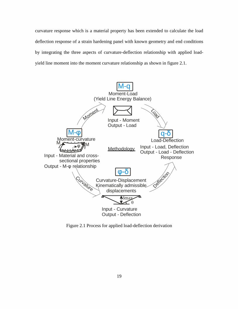
19
curvature response which is a material property has been extended to calculate the load
deflection response of a strain hardening panel with known geometry and end conditions
by integrating the three aspects of curvature-deflection relationship with applied load-
yield line moment into the moment curvature relationship as shown in figure 2.1.
M-φMoment-curvature
Input - Material and cross- sectional propertiesOutput - M- relationshipφ
MMφ
Moment
Moment-Load(Yield Line Energy Balance)
M-q
Curvature
Curvature-DisplacementKinematically admissible
displacements
δmaxθ
φ δ-
Input - MomentOutput - Load
Input - CurvatureOutput - Deflection
Load
Def
lection
Load-Deflection
q- δ
Input - Load, DeflectionOutput - Load - Deflection Response
Methodology
Figure 2.1 Process for applied load-deflection derivation
Page 32
20
Figure 2.2 Construction and applications of SHCC material slabs [11]
2.1 Yield Line Analysis Approach
Yield line design is a well-founded method of designing reinforced concrete slabs, and
similar types of elements. It uses yield line theory to investigate failure mechanisms at
the ultimate limit state. The theory is based on the principle that work done in rotating
yield lines is equal to work done in moving the loads [12][13]. When applying the Work
Method for yield line analysis the calculations for the external work due to loads and the
internal work due to dissipation of energy within the yield lines are carried out
independently. The results are then made equal to each other and from the resulting
equations the unknown, be it the ultimate moment ‘m’ generated in the yield lines or the
ultimate failure distributed load ‘q’ of the slab is evaluated.
The slab is divided into rigid regions that rotate about their respective axes of rotation
along the support lines. If the point of maximum deflection is given a value of unity then
the vertical displacement of any point in the regions is thereby defined. The work done
Page 33
21
due to external loads is evaluated by taking all external loads on each region, finding the
center of gravity of each resultant load and multiplying it by the distance it travels.
The work done due to dissipation of energy is quantified by projecting all the yield lines
around a region onto, and at right angles to, that region’s axis of rotation. These projected
lengths are multiplied by the moment acting on each length and by the angle of rotation
of the region. At the small angles considered, the angle of rotation is equated to the
tangent of the angle produced by the deflection of the region.
2.2 2-D Analysis of Panels for Moment-Load Relationship
Work method has been used to calculate the moment-load relationship for all the basic
configurations of slabs namely square, rectangle and circular with all possible support
conditions. It has been assumed that moment about each point on yield line is consistent
and sagging moment is equal to hogging moment. Yield line formation in square and
rectangular slabs has been assumed to be at 45° to the edges for simplification. General
cases for yield lines not at 45° are also calculated. Load deflection results have been
found out for square and rectangle slabs having uniformly distributed load of magnitude
q and round slabs having a point load acting at center with a magnitude of P. Support
conditions considered include (a) simply supported at the four vertexes in cases of square
and rectangular panels and (b) clamped along the edges.
2.2.1 Case 1 – Applied Load vs. Yield Line Moment Relationship for Square Slabs
Square slab of edge length L is considered here with a distributed load of ‘q’ acting on it.
It is assumed that yield lines are at 45° to the sides and each point on the yield line is
Page 34
22
consistent and under tension. Hogging moment about the yield lines and sagging moment
about the clamped supports are also assumed to be equal in magnitude. Three end
conditions can be considered which are –
i) All sides are simply supported (Case 1.1)
ii) All sides have clamped supports (Case 1.2)
iii) Mixed boundary conditions with two adjacent sides simply supported whereas
other two have clamped supports (Case 1.3)
Case 1.1 – Square Panel with Simply Supported Edges
Plastic analysis approach uses the principal of virtual work to equate the internal and
external work to obtain the collapse load. Similarly the yield pattern is used to define the
potential collapse mechanism of a plate supported along its two or four edges. If the
panel has fixed edges, then the yielding along the edge is also needed to be included in
the calculations.
From the relationship of equating the external work done by loads moving to the internal
energy dissipated by rotations about yield line, one gets:
ext intW W (2-1)
( ) ( )N m l (2-2)
Page 35
23
m0.5L
m
δmax
0.5L
L
A A
Simply supported
θ
L
δmax
Section A-A
Figure 2.3 Simply supported square Panel with (a) yield lines and (b) loading and rotation
conditions through section A-A.
In left hand side, q is the uniformly distributed load and L2/4 is the area of each wedge
(So the equivalent point load is q x L2/4) and δmax/3 is the deflection of the centroid. On
the right hand side, L is the length of the square as the rotations are projected onto the
sides. Rotation angle, θ, can be calculated from geometry shown in figure 2.3(b) as
δmax/0.5L.
2
max max4 44 3 0.5
Lq m L
L
(2-3)
Simplifying equation 2-3 and solving for moment, one gets-
2 248
12 24
L q qLm , m
(2-4)
Page 36
24
Where m is the moment along the yield lines, q is the uniformly distributed load and L is
the length of the square side.
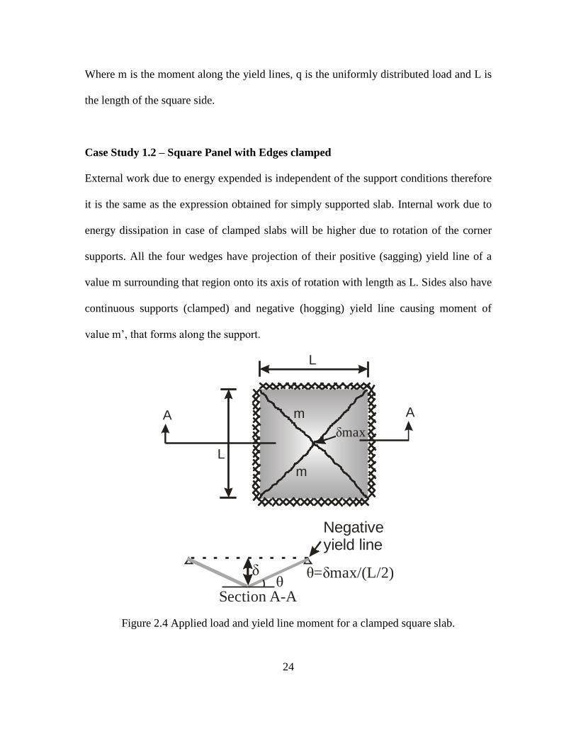
Case Study 1.2 – Square Panel with Edges clamped
External work due to energy expended is independent of the support conditions therefore
it is the same as the expression obtained for simply supported slab. Internal work due to
energy dissipation in case of clamped slabs will be higher due to rotation of the corner
supports. All the four wedges have projection of their positive (sagging) yield line of a
value m surrounding that region onto its axis of rotation with length as L. Sides also have
continuous supports (clamped) and negative (hogging) yield line causing moment of
value m’, that forms along the support.
m
L
L
m
δmax
A A
θδ θ δ= max/(L/2)
Section A-A
Negativeyield line
Figure 2.4 Applied load and yield line moment for a clamped square slab.
Page 37
25
ext int
2
max max max
( ) ( )
4 4 '4 3 0.5 0.5
W W
N m l
Lq m L m L
L L
(2-5)
If one assumes m=m’ (that is the sagging is equal to the hogging moment), one gets:
2 2416 ,
12 48
L q qLm m (2-6)
Case 1.3 for mixed boundary condition can be derived similarly. Results for yield line
moment relationship with applied load for square slabs for various end conditions in
summarized in table 2-1.
Table 2-1 : Applied load – yield line moment relationship for Cases 1.1 to 1.3
Case 1.1
L
L
2
24
qLm
Case 1.2
L
L
2
48
qLm
Case 1.3
L
L
2
36
qLm
Where,
Clamped support
Simply supported
Free support
Moment Rotation
Page 38
26
2.2.2 Case 2- Applied Load vs. Yield Line Moment Relationship for Rectangular
Slabs
Rectangular slab of length ‘a’ and breadth ‘b’ has been considered here and a uniformly
distributed load ‘q’ is acting on it. It is assumed that yield lines are at 45° to the sides and
each point on the yield line is consistent and under tension. Hogging moment at yield line
and sagging moment about the edges are also assumed to be equal in magnitude. Five end
conditions can be considered and their results are summarized in table 2-2.
i) Clamped support about one side and simply supported about other three (Case 2.1)
ii) Clamped support about two adjacent sides and simply supported about other two
adjacent sides (Case 2.2)
iii) Clamped support about three sides and simply supported about one side (Case 2.3)
iv) All 4 sides have same support conditions (Case 2.4)
v) Fixed on three sides and free about one side (Case 2.5)
Derivation for two adjacent edges as clamped and remaining two as simply supported is
presented first. Cases 2.1, 2.3 and 2.4 can be derived similarly.
Case Study 2.2 – Rectangular Slab with two adjacent edges clamped and other two
as simply supported
The slab is divided into rigid regions that rotate about their respective axes of rotation
along the support lines. If the point of maximum deflection is given a value of unity then
the vertical displacement of any point in the regions is thereby defined.
Page 39
27
1
2
3
4
b
Y
X XY
45
a
δ
a
Section X-X
δ
bSection Y-Y
Figure 2.5 Two sides clamped and other two sides simply supported rectangular slab
The expenditure of external loads is evaluated by taking all external loads on each region,
finding the center of gravity of each resultant load and multiplying it by the distance it
travels. Two groups are considered the triangles and the trapezoidal sections:
21 1( ) ( ) 3
3 2 6ext
qbW N q b q a b b a b
(2-7)
In the above expression, the first half of the expression consists of both the triangles
(regions 1 and 3 completely and parts of region 2 and 4). Their area is b2 and therefore
equivalent point load is expressed as qb2 and 1/3 is the deflection of the centroid when
maximum deflection has been assumed as unity. Second half of the expression is
composed of the rectangle at the center which consists of the remaining regions of two
and four.
Page 40
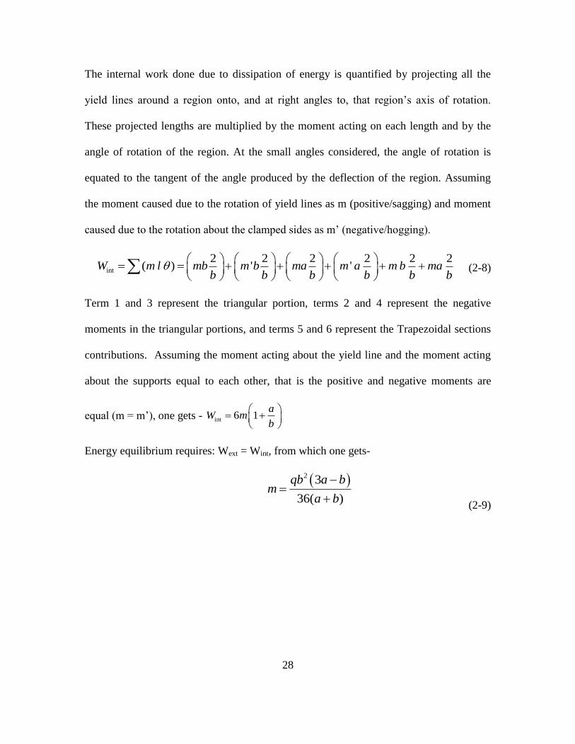
28
The internal work done due to dissipation of energy is quantified by projecting all the
yield lines around a region onto, and at right angles to, that region’s axis of rotation.
These projected lengths are multiplied by the moment acting on each length and by the
angle of rotation of the region. At the small angles considered, the angle of rotation is
equated to the tangent of the angle produced by the deflection of the region. Assuming
the moment caused due to the rotation of yield lines as m (positive/sagging) and moment
caused due to the rotation about the clamped sides as m’ (negative/hogging).
int
2 2 2 2 2 2( ) ' 'W m l mb m b ma m a m b ma
b b b b b b
(2-8)
Term 1 and 3 represent the triangular portion, terms 2 and 4 represent the negative
moments in the triangular portions, and terms 5 and 6 represent the Trapezoidal sections
contributions. Assuming the moment acting about the yield line and the moment acting
about the supports equal to each other, that is the positive and negative moments are
equal (m = m’), one gets - int 6 1a
W mb
Energy equilibrium requires: Wext = Wint, from which one gets-
2 3
36( )
qb a bm
a b
(2-9)
Page 41
29
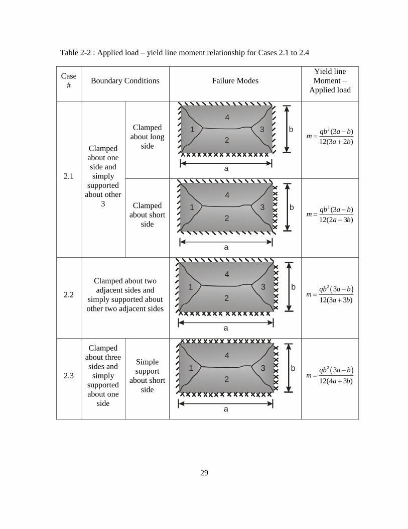
Table 2-2 : Applied load – yield line moment relationship for Cases 2.1 to 2.4
Case
# Boundary Conditions Failure Modes
Yield line
Moment –
Applied load
2.1
Clamped
about one
side and
simply
supported
about other
3
Clamped
about long
side
a
b1
2
3
4
2 (3 )
12(3 2 )
qb a bm
a b
Clamped
about short
side
a
b1
2
3
4
2 (3 )
12(2 3 )
qb a bm
a b
2.2
Clamped about two
adjacent sides and
simply supported about
other two adjacent sides
a
b1
2
3
4
2 3
12(3 3 )
qb a bm
a b
2.3
Clamped
about three
sides and
simply
supported
about one
side
Simple
support
about short
side
a
b1
2
3
4
2 3
12(4 3 )
qb a bm
a b
Page 42
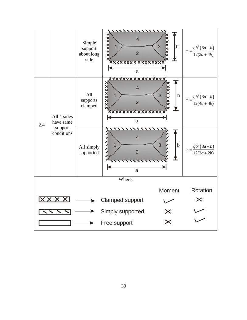
30
Simple
support
about long
side
a
b1
2
3
4
2 3
12(3 4 )
qb a bm
a b
2.4
All 4 sides
have same
support
conditions
All
supports
clamped
a
b1
2
3
4
2 3
12(4 4 )
qb a bm
a b
All simply
supported
a
b1
2
3
4
2 3
12(2 2 )
qb a bm
a b
Where,
Clamped support
Simply supported
Free support
Moment Rotation
Page 43
31
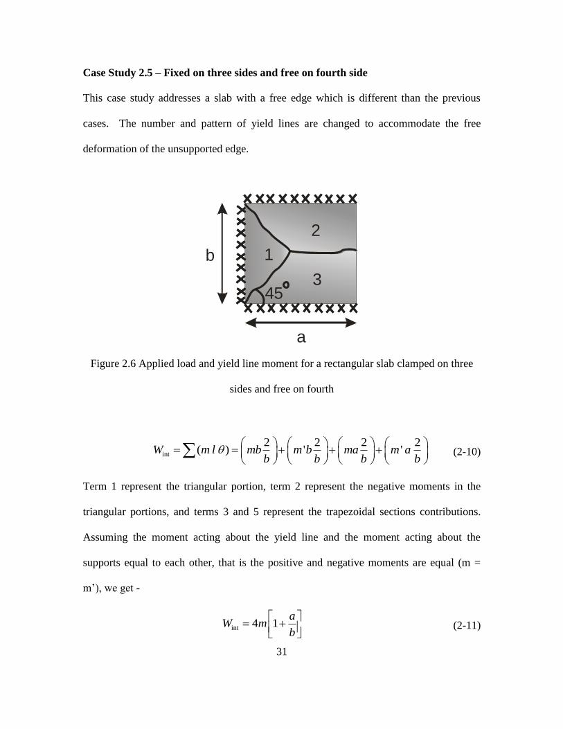
Case Study 2.5 – Fixed on three sides and free on fourth side
This case study addresses a slab with a free edge which is different than the previous
cases. The number and pattern of yield lines are changed to accommodate the free
deformation of the unsupported edge.
a
1
3
2
b
45
Figure 2.6 Applied load and yield line moment for a rectangular slab clamped on three
sides and free on fourth
int
2 2 2 2( ) ' 'W m l mb m b ma m a
b b b b
(2-10)
Term 1 represent the triangular portion, term 2 represent the negative moments in the
triangular portions, and terms 3 and 5 represent the trapezoidal sections contributions.
Assuming the moment acting about the yield line and the moment acting about the
supports equal to each other, that is the positive and negative moments are equal (m =
m’), we get -
int 4 1a
W mb
(2-11)
Page 44
32
21 1( ) ( )
6 2 2 2 6ext
b qb bW N q b q a b a
(2-12)
In the above expression, the first half of the expression consists of both the triangles
(region 1 and parts of region 2 and 3). Their area is 0.5b2 and therefore equivalent point
load is expressed as 0.5qb2 and 1/3 is the deflection of the centroid when maximum
deflection has been assumed as unity. Second half of the expression is composed of the
rectangle which consists of the remaining regions of 2 and 3. Energy equilibrium
requires: Wext = Wint, we get-
2 6
48( )
qb a bm
a b
(2-13)
2.2.3 Case 3 - Applied Load vs. Yield Line Moment for Round Panels
Round panels of radius R is considered here with a point load of ‘P’ acting at the center
on it. Yield lines form a fan shaped design and it is considered that each point on the
yield line is consistent and under tension. Hogging moment along the yields lines and
sagging moment along the supports are also assumed to be equal in magnitude. Two end
conditions can be considered which are –
i) It is simply supported (Case 3.1)
ii) It has clamped support (Case 3.2)
In figure 2.7 if one defines number of cracks as n, then the central angle α can be
calculated as 2π/n. It has been assumed here that when number of cracks, n tends to
infinity, the angle α becomes zero. In case of a simply supported three point ring
specimens, n is taken as 3. Flexural capacity of round slab simply supported (Case 3.1)
Page 45
33
subjected to a center-point loading is shown in figure 2-7. Note that depending on the
number of yield lines, the internal energy dissipation changes.
θ
2R
δ
Section A-A
dα
R
P
Figure 2.7 Principle of virtual work to determine the ultimate load carrying capacity of a
round panel test simply supported in its contour and subjected to center point load
It is however shown that in the case of simply supported round slab, the allowable
applied load can be related to the bending moment capacity which is determined through
laboratory tests on flexural samples [22].
int extW W ;R
intdW MR d M d
Page 46
34
extW P
2
02int extW W M d M P
2
PM
(2-14)
If the support is fixed (Case 3.2), the solution would yield:
2
02 4
int extW W
M d RM M P
(2-15)
4
PM
(2-16)
Table 2-3 : Applied load – yield line moment relationship for Cases 3.1 and 3.2
Case 3.1
2
Pm
Case 3.2
4
Pm
Where,
Page 47
35
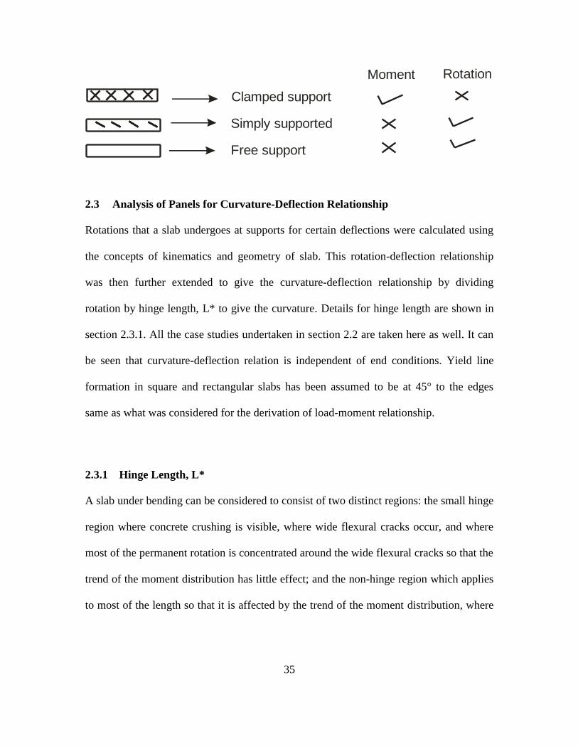
Clamped support
Simply supported
Free support
Moment Rotation
2.3 Analysis of Panels for Curvature-Deflection Relationship
Rotations that a slab undergoes at supports for certain deflections were calculated using
the concepts of kinematics and geometry of slab. This rotation-deflection relationship
was then further extended to give the curvature-deflection relationship by dividing
rotation by hinge length, L* to give the curvature. Details for hinge length are shown in
section 2.3.1. All the case studies undertaken in section 2.2 are taken here as well. It can
be seen that curvature-deflection relation is independent of end conditions. Yield line
formation in square and rectangular slabs has been assumed to be at 45° to the edges
same as what was considered for the derivation of load-moment relationship.
2.3.1 Hinge Length, L*
A slab under bending can be considered to consist of two distinct regions: the small hinge
region where concrete crushing is visible, where wide flexural cracks occur, and where
most of the permanent rotation is concentrated around the wide flexural cracks so that the
trend of the moment distribution has little effect; and the non-hinge region which applies
to most of the length so that it is affected by the trend of the moment distribution, where
Page 48
36
there are much narrower cracks, where, in particular, concrete crushing does not occur
and where standard procedures of equilibrium can be applied [14][15].
Hinge region
Rigid bodyrotation
Rotationθ
θ
Primary flexuralcrack
Figure 2.8 Hinge rotation mechanism (a) Steel fiber reinforced beam (BASF), (b) Rigid
body hinge rotation [16]
Hinge length has been derived to be a function of span, depth or reinforcement [16].
Curvature is a measure of sectional ductility and rotation is a measure of member
ductility. Product of sectional ductility (curvature) and hinge length gives the member
ductility (rotation).
Many researchers have concentrated mainly on quantifying the hinge length, L*
empirically. Some suggested approaches are as shown in table below [16]:
Table 2-4 : Empirically derived hinge lengths
Researcher reference Hinge length (L*) Hinge length variables
Baker [17] k(z/d)1.4
d Span (z), depth (d)
Sawyer [18] 0.25d+0.075z Span, depth
Corley [19] 0.5d+0.2(z/d)√d Span, depth
Mattock [20] 0.5d+0.05z Span, depth
Page 49
37
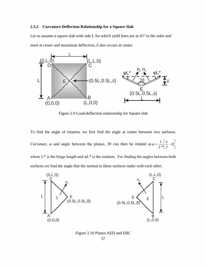
2.3.2 Curvature-Deflection Relationship for a Square Slab
Let us assume a square slab with side L for which yield lines are at 45° to the sides and
meet at center and maximum deflection, δ also occurs at center.
L
δ2θ
(0.5L,0.5L, )δ
φL* φL*
E
n1 n2
L
L
(0,0,0) (L,0,0)
(L,L,0)(0,L,0)
(0.5L,0.5L, )δ
A B
D
E
C
Figure 2.9 Load-deflection relationship for Square slab
To find the angle of rotation, we first find the angle at center between two surfaces.
Curvature, φ and angle between the planes, 2θ can then be related as1
* 2L
where L* is the hinge length and φL* is the rotation. For finding the angles between both
surfaces we find the angle that the normal to these surfaces make with each other.
1L
(0,0,0)
(0,L,0)
(0.5L,0.5L, )δ
A
E
Dn1
3 L
(0.5L,0.5L, )δ
(L,0,0)
(L,L,0)
E
B
Cn2
Figure 2.10 Planes AED and EBC
Page 50
38
For plane # 1 (AED), the normal n1 is the cross product of vectors AE and AD .
21
(0.5 ,0.5 , )
(0, ,0)
ˆˆ ˆ
ˆˆ0.5 0.5 ( ) 0.5
0 0
AE L L
AD L
i j k
n AE X AD L L L i L k
L
Equation of the plane # 1 is given as
2
2
( 0) 0( 0) 0.5 ( 0) 0
( ) 0.5 0
L x y L z
L x L z
(2-17)
For plane # 3 (BCE), the normal n2 is the cross product of vectors BE and BC .
22
( 0.5 ,0.5 , )
(0, ,0)
ˆˆ ˆ
ˆˆ0.5 0.5 ( ) 0.5
0 0
BE L L
BC L
i j k
n BE X BC L L L i L k
L
Equation of the plane # 3 is given as
2
2 2
( ) 0( 0) 0.5 ( 0) 0
( ) 0.5 0
L x L y L z
L x L z L
(2-18)
The angle between planes is the angle between their normal vectors. If A1x + B1y + C1z +
D1 = 0 and A2x + B2y+C2z+D2 = 0 are plane equations, then angle between planes can be
found using the following formula:
1 2 1 2 1 21
2 2 2 1/2 2 2 2 1/2
1 1 1 2 2 2
. . .cos
( ) ( )
A A B B C C
A B C A B C
So the angle between two planes under yielding is given as:
Page 51
39
2 2 4 2 2
2 22 2 4 2 2 4
2 21
2 2
0.25 4cos2 cos( 2 *)
40.25 0.25
1 4cos
2 * 4
L L LL
LL L L L
L
L L
(2-19)
Deflection- curvature relationship is given as:
1 cos2 *
2 1 cos2 *
L L
L
(2-20)
Where δ is the deflection, φ is the curvature, L* is the hinge length and L is the
dimension of the slab.
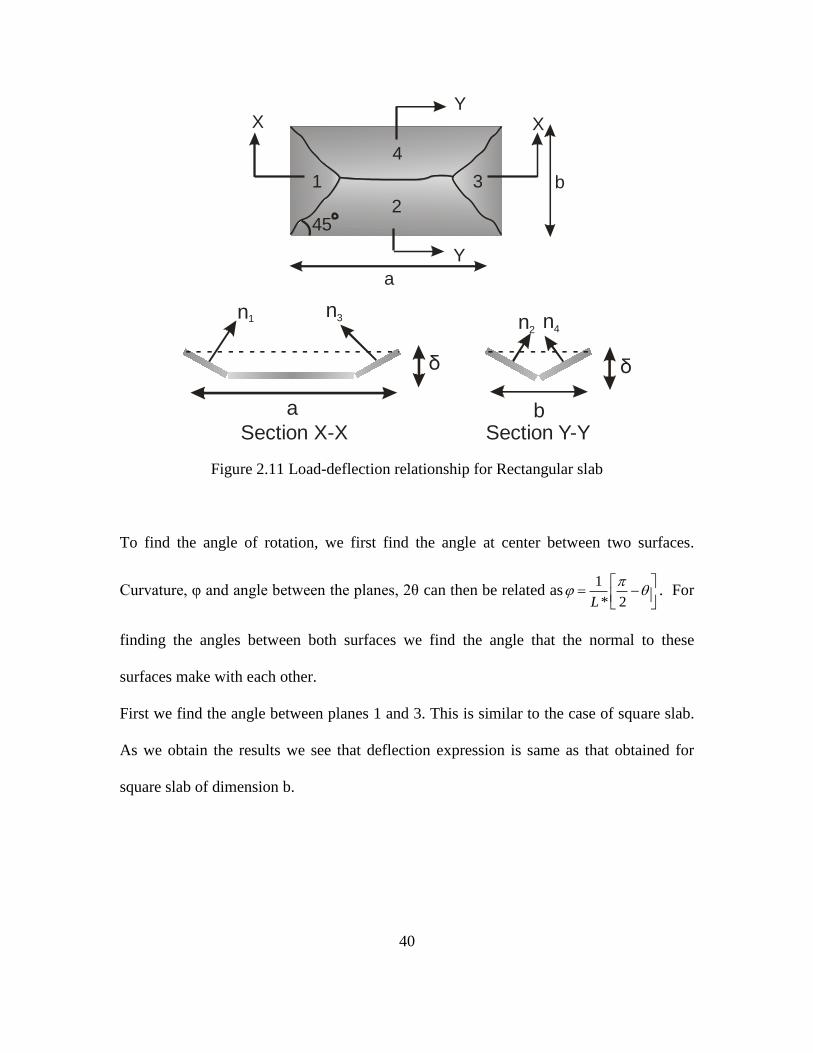
2.3.3 Curvature-Deflection Relationship for Rectangular Slab
Two cases are evaluated, a simplified case where the geometry of deformation is pre-
specified, and a second case where the angle of the deformation is a variable. These are
referred to as case (a) and case (b) and are addressed below.
Case (a) Yield Lines at edges are at 45° Angle to the sides
Let us assume a rectangular slab with length a and breadth b for which yield lines are at
45° to the sides and meet at points as show in the figure 2.11 below and maximum
deflection occurs at that point.
Page 52
40
1
2
3
4
b
Y
X XY
45
a
δ
a
Section X-X
δ
bSection Y-Y
n1n3 n2
n4
Figure 2.11 Load-deflection relationship for Rectangular slab
To find the angle of rotation, we first find the angle at center between two surfaces.
Curvature, φ and angle between the planes, 2θ can then be related as1
* 2L
. For
finding the angles between both surfaces we find the angle that the normal to these
surfaces make with each other.
First we find the angle between planes 1 and 3. This is similar to the case of square slab.
As we obtain the results we see that deflection expression is same as that obtained for
square slab of dimension b.
Page 53
41
1 3b b
(0,0,0)
(0,b,0)
(0.5b,0.5b, )δ (a-0.5b,0.5b, )δ
(a,0,0)
(a,b,0)
K
O
N
P
L
Mn1
n3
Figure 2.12 Planes KON and PLM
For plane # 1 (KON), normal n1 is obtained by the cross product of vectors KO and KN .
2
1
(0.5 ,0.5 , )
(0, ,0)
ˆˆ ˆ
ˆˆ0.5 0.5 0.5
0 0
KO b b
KN b
i j k
n KO X KN b b b i b k
b
Equation of the plane # 1 is given as-
2
2
( 0) 0( 0) 0.5 ( 0) 0
( ) (0.5 ) 0
b x y b z
b x b z
(2-21)
For plane # 3 (PLM), the normal n3 is obtained by the cross product of vectors LP & LM
2
( 0.5 ,0.5 , )
(0, ,0)
ˆˆ ˆ
ˆˆ0.5 0.5 ( ) ( 0.5 )
0 0
LP b b
LM b
i j k
n LP X LM b b b i b bk
b
Equation of the plane # 3 is given as
2
( ) 0( 0) ( 0.5 ) ( 0) 0
( ) 0.5 0
b x a y b b z
b x b z ab
(2-22)
Page 54
42
So the angle between two planes under yielding is given as-
2 2 4 2 2
13 13 2 22 2 4 2 2 4
0.25 4cos2 cos( 2 *)
40.25 0.25
b b bL
bb b b b
Deflection in terms of curvature can be simplified as:
13
13
1 cos2 *
2 1 cos2 *
Lb
L
(2-23)
It is known by symmetry that 13 24
Similarly, we find the angle between planes 1 and 4 by the same procedure –
0.5b
a
(0.5b,0.5b, )δ
N(a,b, )0
(a-0.5b,0.5b, )δ
41b
(0,0,0)
(0,b,0)
(0.5b,0.5b, )δ
K
O
Nn1
n4
(0,b, )0
O P
M
Figure 2.13 Planes KON and NOPM
For plane # 1 (KON), the normal n1 by the cross product between the vectors KO & KN
1
(0.5 ,0.5 , )
(0, ,0)
ˆˆ ˆ( ) ˆˆ0.5 0.5 ( )
20 0
KO b b
KN b
i j kb b
n KO X KN b b b i k
b
Equation of the plane # 1is given as
Page 55
43
2
2
( 0) 0( 0) 0.5 ( 0) 0
( ) 0.5 0
b x y b z
b x b z
(2-24)
For plane # 4 (NOPM), the normal n4 is the cross product of vectors NO and NM
4
( 0.5 ,0.5 , )
( ,0,0)
ˆˆ ˆ
ˆˆ0.5 0.5 ( ) (0.5 )
0 0
NO b b
NM a
i j k
n NO X NM b b a j ab k
a
Equation of the plane # 4 is given as
( ) ( 0.5 ) ( 0) 0
( ) 0.5 0
a y b a b z
a y ab z ab
So the angle between two planes under yielding is given as-
3 2
14 14 2 22 2 4 2 2 2 2
0.25cos2 cos( 2 *)
40.25 0.25
ab bL
bb b a a b
21
14 2 2
1cos
2 * 4
b
L b
(2-25)
Deflection in terms of curvature can be simplified as:
14
14
1 cos2( *)
2 cos2( *)
Lb
L
(2-26)
By the geometry of slab we know that 12 14 23 34 .
Page 56
44
1
3
2
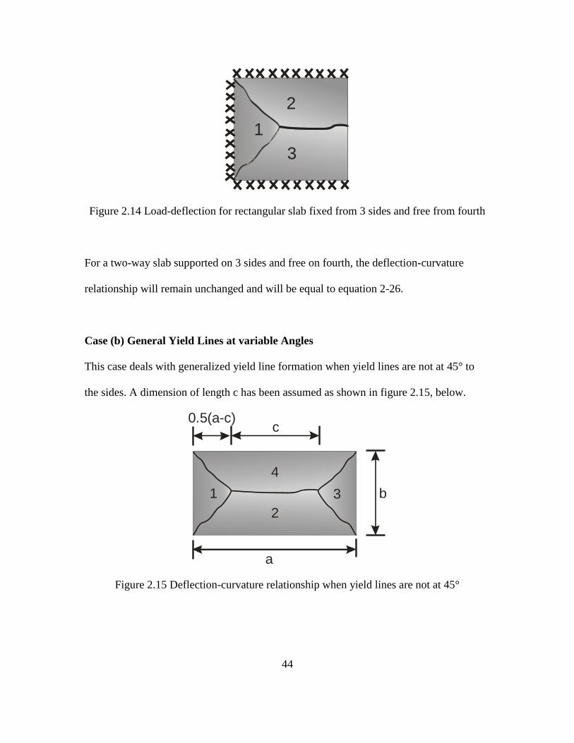
Figure 2.14 Load-deflection for rectangular slab fixed from 3 sides and free from fourth
For a two-way slab supported on 3 sides and free on fourth, the deflection-curvature
relationship will remain unchanged and will be equal to equation 2-26.
Case (b) General Yield Lines at variable Angles
This case deals with generalized yield line formation when yield lines are not at 45° to
the sides. A dimension of length c has been assumed as shown in figure 2.15, below.
1
2
3
4
b
a
c0.5(a-c)
Figure 2.15 Deflection-curvature relationship when yield lines are not at 45°
Page 57
45
1 3b b
(0,0,0)
(0,b,0)
(0.5(a-c),0.5b, )δ (0.5(a+c),0.5b, )δ
(a,0,0)
(a,b,0)
K
O
N
P
L
M
n1
n3
For plane # 1 (KON), the normal n1 is the cross product of vectors KO and KN .
1
(0.5( ),0.5 , )
(0, ,0)
ˆˆ ˆ
ˆˆ0.5( ) 0.5 0.5( )
0 0
KO a c b
KN b
i j k
n KO X KN a c b b i a c bk
b
Equation of the plane # 1 is given as
( 0) 0( 0) 0.5( ) ( 0) 0
0.5( ) 0
b x y a c b z
b x a c bz
(2-27)
For plane # 3 (PLM), the normal n3 is the cross product of the vectors LP and LM .
2
(0.5( ),0.5 , )
(0, ,0)
ˆˆ ˆ
ˆˆ0.5( ) 0.5 ( ) 0.5( )
0 0
LP c a c
LM c
i j k
n LP X LM c a b b i c a bk
b
Equation of the plane # 3 is given as
( ) 0( 0) 0.5( ) ( 0) 0
( ) 0.5( ) 0
b x a y a c b z
b x a c bz ab
(2-28)
So the angle between two planes under yielding is given as-
Page 58
46
2 2 2 2 2 2
2 2 2 2 2 2
0.25( ) 4 ( )cos2 cos( 2 *)
0.25( ) 4 ( )
b a c b a cL
b a c b a c
(2-29)
Deflection in terms of curvature can be simplified as
13
13
1 cos2 *1( )
2 1 cos2 *
La c
L
(2-30)
By defining c a
13
13
1 cos2 *(1 )
2 1 cos2 *
La
L
(2-31)
2.3.4 Curvature-Deflection Relationship for Round Panels
Assume a round slab with radius R for with yield lines are originating at the center and
extending till the boundary of the slab as shown in the figure 2.16 below and maximum
deflection occurs at that center [22].
Figure 2.16 Load-deflection relationship for Circular slab
From figure 2.16 crack segment 1 rigidly rotate around the axis AB.
Page 59
47
sin(30) 1
2
C BC R
AO R
2
C
Thus, the deflection at the edge (point C) is half that of the center. Assume each crack
segment is rigid and it rotates around the crack axis represented by vectors OC , OD and
OE as shown in Fig. 2.23.
( ,0,0.5 )OC R
( sin(30), cos(30),0.5 )OD R R
( sin(30), cos(30),0.5 )OE R R
The vectors normal to crack segment 1 and 2 can be found by cross product of the two
adjacent vectors.
21
3 3 3, ,
4 4 2n OD OC R R R
(2-32)
22
3 3 3, ,
4 4 2n OC OE R R R
(2-33)
The angle of curvature φ between segment 1 and 2 is the angle between these two normal
vectors, determined by the dot product.
2 21 11 2
2 21 2
1 1 2cos cos
* * 2
n n R
L n n L R
(2-34)
Deflection in terms of curvature can be simplified as:
22 (1 cos *)
(1 2cos *)
R L
L
(2-35)
Page 60
48
2.4 Applied load - Deflection Response
Algorithm to calculate load deflection response for limit state analysis using yield line
theory was developed by integrating the three aspects of curvature-deflection relationship
with applied load-yield line moment into the moment curvature relationship. As shown in
figure 2.17 all the components of the algorithm are defined and one can develop a step
wise simplified approach. Using the simplified model for strain hardening cement
composites model (Section 1.2) one can approach the problem in the following manner:
i. For a given cross section and material properties and using M’ – φ’ relation
from expressions in table 1-2 calculate normalized moment for discrete number
of curvature values. Using the normalized moment relation 2' / 6crM M bh
and normalized curvature as ' 2 /cr d , the moment-curvature response of
the cross-section is obtained.
ii. Using a discrete number of moment magnitudes along the moment curvature
diagram, a load vector is generated using the relationship between moment and
load for the panel configurations as derived by the yield line methodology in
section 2.2.
iii. The slab is segmented into finite sections and maximum deflection is
calculated using the relationship between curvature and deflection as derived in
section 2.3.
iv. This procedure is applied at each step until a complete load deflection response
is obtained for the corresponding moment curvature relationship.
Page 61
49
Step 5 – Correlate the load calculated from step 3 with deflection from step 4 to get the load-deflection
relationship.
Step 4 – Calculate deflection corresponding to each curvature value by using the deflection-curvature
relationship as derived in section 2.3.
Step 3 – Calculate load corresponding to each moment value by using the load-moment
relationship as derived in section 2.2
Step 2 – Convert normalized moment (M’) to moment by using the relationship – M = M’Mcr and normalized curvature (φ’) to curvature by φ=φcrφ’
Step 1 – Calculate the material property of moment-curvature relation from M’-φ relationship from Table
1-1 for strain hardening composites for a discrete number of points.
Figure 2.17 Flowchart for the derivation of applied load-deflection relationship for SHCC
materials
2.5 Shortcomings of the Methodology - Increased Load Bearing Strength at
Large Vertical Displacements
Concrete slabs at large vertical displacements could support loads considerably greater
than those calculated using the yield-line approach [21]. The mechanism for supporting
the load was shown to be tensile membrane action, which could form within the slab
irrespective of whether it was restrained or unrestrained horizontally at its boundaries.
For a slab which was unrestrained around its boundaries, compressive in-plane membrane
Page 62
50
forces were shown to form within the depth of the slab around its perimeter, and these
provided the required support to the in-plane tensile membrane forces in the central
region of the slab. The mechanism is shown below in the figure 2.18.
Compression zone(’ring’)
Tension zone
Figure 2.18 Different zones for slabs subjected to large displacements [21]
2.6 Comparison with Experimental Data
2.6.1 Data Set 1
Experimental results from round panel tests analyzed by Soranakom et. al are considered
first [22]. The parameter based fit equations for moment curvature relationship are used
for stages 2.1 and 3.1 which were obtained by curve fitting the simulated response from
the closed form derivations and are applicable within 1% accuracy of the closed form
results. Tabix steel fibers are used as the reinforcement in these SHCC material slabs.
Page 63
51
Diameters of experimented slabs were 2000 mm and 1500 mm. Simulation was done in
following steps:
(a) Step 1 - Calculate the moment-curvature relationship using the strain hardening
cement composites model as discussed in section 1.2 for all the stages. Assume that this
material is governed by following stages –
(i) Stage 1 – Elastic compression, elastic tension
(ii) Stage 2.1 – Elastic compression, tension hardening
(iii) Stage 3.1 – Elastic compression, tension softening.
Stages 2.2 and 3.2 are not considered here as it has been observed that tension governs
the design instead of compression.
The following parameters are proposed for the design of these samples:
η =Ratio of post crack stiffness to elastic stiffness (Ecr/E) = 0.01
γ= Ratio of stiffness in tension and compression (Ec/E ) = 1
µ = Post tensile strain capacity, cst
crE
= 0.6.
Strain capacity parameter, α= trn
cr
, α=10. This parameter represents the ultimate strain
capacity in the section with the reduced tensile stiffness. The following simplified
relations are obtained after the closed form solutions to the moment curvature
relationship are subjected to a polynomial curve fit approach. For a homogeneous and an
isotropic plate, the bending stiffness, D will be given as EI/ (1-υ2). As square of poisson’s
ratio will be a very small number, therefore elastic stiffness can be approximated as EI.
Page 64
52
M = EI(φ) (Stage 1)
For stages 2.1 and 3.1, while the closed form equations can be easily used individually, it
may be easier to apply a curve fit to the entire relationship between normalized moment
(M’) and normalized curvature (φ’) in these two regions as:
' 1.342 0.371 'M (Stage 2.1)
5 4 3 2' 2.34 ' 0.0017 ' 0.0481 ' 0.5551 ' 3.9454M e (Stage 3.1)
(b) Step 2 - Convert from the normalized moment and curvature for stages 2.1 and
3.1 to moment-curvature by factoring in the cracking moment and curvature
corresponding to first cracking.
2
6
2' '
’ ' cr
crcr
cr
bhM M M
d
M
For radius as 1000 mm, thickness 200 mm, cracking strain as 100µstr and cracking stress
as 3 MPa, one obtains for stage 2:
6 6 22(100)(10 )1.342 0.371
0.
3(10 )(4)(0
2
.2)
6M
51.342 0.371 0.0017.98 10 N m
Similar expression can also be calculated for stage 3.1.
(c) Step 3 - Since the sample is simply supported on all sides subjected to point load,
from section 2.2 one can use the following moment-load relationship as equation 2-4.
2
Pm
Case (3.1)
Page 65
53
(d) Step 4 – From section 2.3 the appropriate expression for curvature-deflection
relationship for a square slab is given by equation 2-35 as below is used. From table 2-4,
it can be seen that hinge length can be approximated to lie in the range of 10 mm to 50
mm. Hinge length is assumed as 10 mm for simplification. Figure 2-21 shows the effect
of hinge length
2(1 cos *)
(1 2cos *)
LR
L
(e) Step 5 – Calculate the load-deflection result using the results from steps 3 and 4.
From figure 2.20 it can be seen that only stages 1 and 2.1 are applicable and material
does not go into tension softening corresponding to stage 3.1 as which can be attributed
to high volume fraction of fibers.
Figure 2.19 Strain hardening-softening tension model with the parameters used for fitting
the model (η=0.01, µ=0.6, α=5)
Page 66
54
Figure 2.20 Comparison of experimental results with methodology for round panels
Figure 2.21 shows the effect of hinge length, L* on the load-deflection response. From
figure 2.21 it can be seen that for a strain capacity parameter, α value of 100, stage 3.1
can be delayed which is applicable for this dataset.
Page 67
55
Figure 2.21 Effect of hinge length on simulated results
2.6.2 Data Set 2
Experimental results for square slabs are considered in a study published by Khaloo and
Afshari here [ 23 ]. Results were digitized for comparison. The parameter based fit
equations for moment curvature relationship are used for stages 2.1 and 3.1 which were
obtained by curve fitting the simulated response from the closed form derivations and are
applicable within 1% accuracy of the closed form results. Span of slabs was 680 mm x
680 mm with 80 mm thickness. Original test data is as shown below:
Page 68
56
Figure 2.22 Experimental results for square slabs [23]
Steps for simulation are shown below -
Step 1 – Similar to data set 1, if one starts with calculating the moment curvature
relationship using the strain hardening cement composites model as discussed in section
1.2. One can find the moment curvature response for the stages 1, 2.1 and 3.1.
The following parameters are proposed for the design of these samples –
Ratio of post crack stiffness to elastic stiffness (Ecr/E), η = 0.01
For strain hardening materials (γ = Ec/E), use equal stiffness in tension and compression
γ=1.
Post tensile strain capacity, cst
crE
, µ=0.4.
Strain capacity parameter, trn
cr
, α=10. This parameter represents the ultimate strain
capacity in the section with the reduced tensile stiffness. The following simplified
relations are obtained after the closed form solutions to the moment curvature
Page 69
57
relationship are subjected to a polynomial curve fit approach. For a homogeneous and an
isotropic plate, the bending stiffness, D will be given as EI/ (1-υ2). As square of poisson’s
ratio will be a very small number, therefore elastic stiffness can be approximated as EI.
M = EI(φ) (Stage 1)
For stages 2.1 and 3.1 we get relationship between normalized moment (M’) and
normalized curvature (φ’) which we convert to moment-curvature as shown in step 2.
' 1.342 0.371 'M (Stage 2.1)
4 4 3 2' 1.933 ' 0.01435 ' 0.3862 ' 4.4898 ' 20.2440M e (Stage 3.1)
Step 2 – We then convert the normalized moment and curvature for stages 2.1 and 3.1 to
moment-curvature by factoring in the cracking moment and curvature corresponding to
first cracking.
2
6
2' '
’ ' cr
crcr
cr
bhM M M
d
M
For clear span as 680 mm, thickness 80 mm, cracking strain as 40µstr and cracking stress
as 0.6 MPa, we get –
For stage 2.1 we get –
6 6 22(40)(10 )1.342 0.371
0.
0.6(10 )(4)(0.2)
0 68M
51.342 0.371 0.0011.59 10 N m
Similar expression can also be calculated for stage 3.1.
Page 70
58
Step 3 - The end conditions are simply supported on all sides. From section 2.2 we get
the moment-load relationship as-
For point load - 24
qm (Case 1.1)
Step 4 – From section 2.3 the appropriate expression for curvature-deflection relationship
for a square slab is given by equation 2-20 as below is used. From table 2-4, it can be
seen that hinge length can be approximated to lie in the range of 10 mm to 25 mm. Hinge
length is assumed as 10 mm for simplification.
1 cos2 *
2 1 cos2 *
L L
L
Step 5 – Calculate the load-deflection result using the results from steps 3 and 4.
Figure 2.23 Comparison of experimental results with the methodology for square panels
Page 71
59
2.7 Interaction of the Different Tensile Zones on the Load-Deflection Response
of the Panels Based on the Moment-Curvature and Limit Analysis
Assuming that the kinematics of the problem do not change as the sample cracks and
deforms, one can start the problem from the elastic response using the panel’s initial
bending stiffness D as, D= EI/(1-υ2). This example illustrates how load deflection
response can be simulated for a strain hardening material with known material properties
such as moment-curvature relationship, cracking moment, hinge length, geometry and
end conditions. Additionally the formulation addresses the interactions between the
different modes of failure in stages 2.1 and 3.1 of the model presented in section 1.2.
Instead of using various criteria for failure, both mechanisms of 2.1 and 3.1 are used
independently and the results superposed in order to show the transition from one mode
to the other. Let us assume a square slab of length 4000 mm, thickness 200 mm, cracking
stress 1 MPa and factor η (Ecr/E) as 0.01.
4000
mm
4000 mm
4000 mm
δ2θ200 mm
q N/m2
Simply supported
Yieldlines
φL* φL*
Figure 2.24 Problem parameters
Page 72
60
Step 1 – The starting point of the procedure is the moment curvature relationship using
the strain hardening cement composites model as discussed earlier obtained for all the
stages defined as:
(i) Stage 1 – Elastic compression, elastic tension
(ii) Stage 2.1 – Elastic compression, tension hardening
(iii) Stage 3.1 – Elastic compression, tension softening.
Stages 2.2 and 3.2 are not considered here under the assumption that tension governs the
design instead of compression. They can be easily added to the formulation. In the
present example the following parameters for design are used:
η = Ratio of post crack stiffness to elastic stiffness (Ecr/E) = 0.01
γ = Tensile to compressive stiffness ratio, (Ec/E) = 1
µ= Post tensile strain capacity, cst
crE
=0.6
α=Strain capacity at the ultimate tensile strength, trn
cr
=10
The following simplified relations obtained by curve fitting the results of moment
curvature relationship in accordance with the procedures developed by Mobasher [24] are
used:
For a homogeneous and an isotropic plate, the bending stiffness, D will be given as EI/
(1-υ2). As square of poisson’s ratio will be a very small number, therefore elastic bending
stiffness can be approximated as EI.
M = EI(φ) Stage 1
Page 73
61
For stages 2.1 and 3.1 we get relationship between normalized moment (M’) and
normalized curvature (φ’) which we convert to moment-curvature as shown in step 2.
M’ = 1.342 0.371 ' Stage 2.1
5 4 3 2' 2.34 ' 0.0017 ' 0.0481 ' 0.5551 ' 3.9454M e Stage 3.1
Step 2 – The normalized moment and curvature for stages 2.1 and 3.1 are scaled to
sectional moment-curvature by incorporating the moment and curvature corresponding to
first cracking point.
2
6
2' '
’ ' cr
crcr
cr
bhM M M
d
M
For stage 2.1, and using a length of 4000 mm, thickness 200 mm, cracking strain as
100µstr and cracking stress as 1 MPa, one obtains:
6 6 2
5
(10 )(4)(0.22(100)(10 )1.342 0.371
0.2
1.342
)
6
2.6 0.371 0.006 101
M
N m
Similar expression can also be calculated for stage 3.1.
Step 3 – The load-moment relationship can be obtained from the equations 2-4. In this
case, assume that the end conditions are simply supported on all sides. From section 2.2
the moment-load relationship is obtained as:
2
24
qLm (Uniformly distributed load)
Page 74
62
Figure 2.25 Moment-curvature relationship for SHCC
Figure 2.26 Moment-load response for (a) uniformly distrib. load, (b) point load at center.
Step 4 –Computation of Deflection-rotation response is obtained from section 2.3 where
one obtains the expression for a square slab.
Page 75
63
1
2 21 cos2
4(1 cos2 )
L
Figure 2.27 Deflection-curvature relationship
Step 5 – Finally one can calculate the load-deflection using the results from steps 1 to 4.
Figure 2.28 (a) Applied load-deflection relationship
Page 76
64
Load-deflection response shown in figure 2.28 can then be integrated to give a response
as shown in figure 2.29.
Figure 2.29 (b) Equivalent applied load-deflection relationship
2.8 Post-Crack Analysis of ASTM C1550 Test results using the Proposed Yield
Line Load-Deflection Model
The proposed methodology can be used to define an effective stiffness of cracked
concrete slabs under flexure. Using the moment rotation curve, one can introduce an
effective stiffness using a tangent stiffness of approach to obtain the instantaneous
stiffness of the fully cracked panel. The test results of ASTM C1550 [25] are used in
order to verify the proposed methodology. Samples are tested using a round panel of
dimensions 800 mm diameter and 75 mm thickness, that is resting on three pivotal points
and subjected to a point load and were made from synthetic macro fibers.
Page 77
65
Moment deflection relationship was proposed by Johansen [ 26 ] which can also be
extended to calculate the load deflection response by implementing applied load and
yield line moment relationship. Johansen showed that by a suitable choice of a one-way
strip taken out of any slab with a uniformly distributed load, restrained or simply
supported and analyzed using the yield line theory, the deflection, δ, could be estimated
by the formula:
2
8
uM L
EI (2-36)
This method can implemented to SHCC using the tri-linear model as discussed in chapter
1 with the objective of fitting the results from full scale tests. The yield line method
shows to be highly effective in the design of 2-D plane members subjected to bending,
owing to its handiness and closeness to the actual structural behavior. Inserting the
moment in terms of point load as found in equation number 2-14, we get the deflection
load relationship as –
22
2
8 16
PR
PR
EI EI
(2-37)
The stiffness parameter in the load deflection expression has been modified to
accommodate the post peak behavior as defined in the SHCC model in chapter 1. The
final equation takes the form as:
'
'
creff
cr
M MEI
(2-38)
2
16 ';
'
creff eff
cr
M MP k k
R
(2-39)
Page 78
66
As this is a yield-line type analysis, therefore it is applicable only after the formation of
yield lines. By using this approach, one cannot fit the peak response. The comparison
shows that the yield line method provides a good estimation of the load bearing capacity
of the slab after the peak load failure (formation of yield lines).
Figure 2.30 Round panel tests (a) Test set up, (b) Comparison between the experimental
data and simplified model based on Johansen’s formula
The results from the equation 2-39 above and test results on a SHCC material circular
slab are compared in figure 2.30. As it can be seen that initially yield line approach can
only be applicable after the post peak phase which is after the formation of yield lines.
Page 79
67
3. CHAPTER 3 - SHEAR PROPERTIES OF TEXTILE REINFORCED
CONCRETE BY MECHANICAL TESTS AND DIGITAL IMAGE
CORRELATION
The study of textile reinforced concrete (TRC) composites has progressed since the mid-
1990s. Researchers have become increasingly interested in TRC composites because of
their wide range of rheological, mechanical, chemical and aesthetic characteristics [27].
This interest is also related to the diversity of TRC applications, primarily for light work
and potentially for structural work. For structural applications, TRC is primarily used
under tensile solicitation (e.g. integrated formwork elements and repair and/or
strengthening of reinforced concrete structures). However, the deformation behavior of
the composite is greatly associated with the relative motion, thus primarily depending on
the shear behavior of the fabric, which determines its performance properties when
subjected to a wide variety of complex deformations, as well as its conformance to the
required shape. Therefore, the in-plane shear strain can influence the behavior of certain
TRC structures and can lead to their failure. The estimation of TRC’s shear resistance
contribution in design, which is presently deducted from TRC’s tensile property, requires
various investigations since the shear resistance mechanism is usually complicated [28].
Thus, to broaden the spectrum of TRC applications and get more accurate shear
properties, an experimental study was conducted to characterize the in-plane shear
behavior of TRC composites.
Page 80
68
For textile reinforced concrete there is no set standard test method for determining the in-
plane shear behavior. There are three main known techniques used to measure shear
compliance, namely the Direct Shear Force Measurement (DSFM) method, the Bias-
Extension test method, and the picture frame test method. Literature search indicated that
the bias extension approach usually brings out a complex combination of shear and
tension which makes it difficult to isolate the shear deformation in the test and hence
complicates the characterization of pure shear behavior [29]. In the picture-frame shear
test, a sample is clamped within a square frame hinged at each corner. The two
diagonally opposite corners are then displaced using a mechanical testing machine. A
uniform shear deformation state is produced. Therefore pictures frame was used to
impose a pure in-plane shear kinematics to the specimen.
Figure 3.1 Methods of measuring shear force – (a) direct shear force measurement and (b)
picture frame test
Page 81
69
3.1 Experimental Program
A partial fly-ash substituted cement based mix design was used in the pultrusion process
for making the samples as described in section 1.3. Mixture proportions of the ingredients
are listed in table 3-1. Constituents of the mix are weighted and mixed using standard
Hobart mixer.
Figure 3.2 Standard Hobart mixer
Table 3-1 : Mix design
Material (each batch) Percentage (by weight)
Cement 49.20
Fly ash 24.60
Water ~ Room temperature 25.80
Super plasticizer 0.01
Page 82
70
3.2 Shear Test Procedure and Instrumentation
The specimen was clamped on the picture frame fixture by bolting the three holes on all
four sides and the bolts were carefully tightened. It is very important that a constant
amount of force should be applied when tightening the bolts. Loose pinning of the sample
edges in the clamps may fail to induce the required kinematics, whereas tight clamping of
the sample edges can cause spurious results if the sample is even slightly misaligned [30].
Then the whole fixture with attached specimen was placed onto the hydraulic grips of the
testing machine, and connected with the crossheads. Top hydraulic grip was attached to
the load cell to measure the force and bottom hydraulic grip was attached to the actuator.
After that, the distance between the upper and lower crossheads was adjusted, and it was
ensured that the angles between the arms of fixture were 90° [31]. The current distance
was set as the original reference value, i.e., the displacement is made zero, in computer,
so that later on, all the experiments can automatically begin from this zero point. Also,
the force was adjusted to be zero at this position. Loading was at a designated speed
(2.5mm/min) by moving the actuator down until the end of the test. Digital data
acquisition for the instron machine collected data at every 0.5 seconds.
After several trials of this test, the average value of load, at each displacement point was
calculated. The load-displacement relationship of the empty frame was also calculated by
following the same procedure without the specimen. This is to record the load-
displacement behavior of the empty fixture under the same condition as in the real shear
experiment to calculate the resistance provided by the frame.
Page 83
71
Figure 3.3 Test set-up
Simultaneously, the photos were taken of the deforming specimen at a constant rate of 10
frames per second. This is the slowest speed for the high speed phantom cameras that
were used. At the end of every test, the crosshead was recovered to the zero point again.
The deformed specimen was taken down and a new sample was clamped to do another
round of test.
Page 84
72
LVDT & servo-valve
Actuator
Lower hydraulic grip
Multiplier links
BearingClamping plate
Slot
Upper Hydraulic grip
Load Cell
Figure 3.4 Schematics of test set-up
The rig is jointed at each corner such that its sides can rotate and the interior angle
between adjacent sides can change. The initially square frame thus becomes of rhomboid
(or diamond) shape. Figure 3.5 show the different stages during the experiment showing
the sample going from initial configuration of square to rhomboid. Material inside the rig
is subjected to pure shear deformation kinematics. The force required to deform the
material is recorded at the load cell connected to the top crosshead. From this information
the shear force (or stress) can be determined as a function of shear angle and shear angle
rate.
Page 85
73
Figure 3.5 Different stages of experiment
3.3 Data Reduction Methods
3.3.1 Determination of Shear Force
L fram
e
L ampl
ifier
A
B
C
D
E F
P
Figure 3.6 Schematics of picture frame tests
Page 86
74
B
C
RBxx
FLOAD-BC
F shear
φ
RByy
RCxx
Figure 3.7 Free body diagram for link BC
The free body diagram of frame link BC is as shown in figure 3.7. All joints are free for
motion. Using symmetry, it can be determined that the force applied on joint C from links
CD and BC is equal and opposite in x-direction and equal and in same direction in y-
direction [28][31].
B
C
RBxx
FLOAD-BC
F shea
r
φ
RByy
RCxx
Figure 3.8 Simplified Free body diagram for link BC
Page 87
75
In this study a simplified loading mechanism as shown in figure 3.8 has been assumed to
find a direct relationship between the load recorded by the data acquisition system and
shear force. Stress contours from image analysis or finite element modelling need to be
used for actual mechanisms.
Using the free body diagram of link BC and performing static analysis for equilibrium in
y direction, one gets:
cos
Load BCshear
FF
(3-1)
Reaction at B in y-direction, RByy has been assumed to be equal to zero because the joint
B is free for motion as the resistance provided by empty frame was less than 1% of the
results. Reaction at B in x-direction can be attributed to resistance to the compressive
force from the samples. As FLoad-BC and FLoad-CD will be equal due to symmetry and their
sum will be equal to the load recorded by the data acquisition system, shear force
expression will be given as:
2cos
Loadshear
FF
(3-2)
Shear stress, τxy can then be found by dividing shear force by the cross-sectional area of
material with area parallel to the applied force vector which is the product of thickness
and length of square.
3.3.2 Determination of Shear Angle
Initial configuration of the frame at the start of the test is as shown below. All the sides of
frame are perpendicular to each other. Distance between top and bottom vertex is L√2.
Page 88
76
Top is fixed to the load cell and bottom is pulled by the machine. Frame goes from a
square configuration to rhomboid (diamond like) configuration.
π/2
L√2
Figure 3.9 Initial configuration
Figure 3.10 below shows the configuration after a certain displacement of D and the
distance between the top and bottom vertex is now L√2+D. The frame angle, ϕ which
was initially π/2 has changed now. Frame angle can be related to shear angle, θ (α+β) by
the relation 22
.
L√2+D
2ϕα
β
ϕLL/√2+D/2
Figure 3.10 Configuration after a displacement of D units
Frame angle, ϕ after displacement D can be calculated from the figure 3.10 as:
1 1cos
22
D
L
(3-3)
Page 89
77
The material shear angle can be calculated from the crosshead displacement using:
1 12 2cos
2 2 22
D
L
(3-4)
Where D is the crosshead displacement, L is the side length of the picture frame (i.e.
distance between bearings) and Φ is the frame angle. It should be noted that the frame
had an amplifier link, therefor the displacement of the sample D was a factor of the ratio
of length of frame and length of amplifier link.
3.3.3 Determination of Shear Strain
A B
CD
a
b
c
d
α
β
X
Y
u(x)
u(y)
Figure 3.11 Theoretical shear strain
Engineering shear strain can be defined from figure 3.11 as the change in angle between
the sides AB and AD. Therefore, the shear angle is same as the shear strain
y xxy
u u
x y
. The shear strain is equal to shear angle and can be calculated
Page 90
78
from the geometry of sample and displacement induced by actuator on the sample by the
formula as-
1 12cos
2 22xy
D
L
(3-5)
It should be noted that this expression is only applicable for small displacements and
small rotations as the approximations 1; 1yx
uu
x y
and ;
yxuu
x y
have been
assumed. Also this approach assumes that the displacement, D of the actuator is the
displacement of the sample, which is not true. Using three dimensional digital image
correlation techniques, it will show the difference between the shear angle, which is the
shear strain for small scale displacements and the shear strains as observed through image
analysis. For this reason the shear strain calculated from the equation 3-4 has been
referred as shear angle only throughout this thesis.
3.1 Digital Image Correlation (DIC) method
3.1.1 Introduction and applications
In the past decades, contacting deformation measurement techniques and devices
including linear variable differential transformer (LVDT) and electrical-resistance strain
gage were widely used in the field of experimental mechanics. However, both LVDT and
strain gage only measure the displacement or strain at isolate locations that the
deformation behavior of materials are not fully investigated [ 32 ]. Additionally, the
experiments are limited by disadvantages of these methods including the effective
working range, which results in varieties types of LVDT and strain gages; environments
Page 91
79
such as the effect of temperature on strain gages; extra effort in experiment preparation
like soldering, wiring and mounting; extra cost due to the disposable devices. Thus there
is a demand on newer measurement techniques. Optical techniques such as moiré
interferometry [33], holography [34] and speckle inteferometry [35] have been proven to
be matured techniques to analyze macroscopic parameters and are being applied
successfully in many different applications. However, all the interferometric techniques
have stringent requirements for system’s stability. Moreover, the processing of fringe
patterns is laborious and time-consuming [36]. This technical difficulty has raised many
researchers’ attention and computerized procedures [ 37 ] have been developed to
automate the processing of the data from the fringe patterns.
In the thirty years, a non-contacting optical technique, digital image correlation, has been
developed by Sutton et al. [38, 39, 40, 41] and Bruck, et al. [42]. As of recent years, DIC
was widely applied to measurement of displacements and strains in many fields such as
material science, mechanical engineering, biomechanics and structural engineering. The
applications include strain measurements for anisotropic plastic deformation during
tension testing [43], strain measurements in a CuAlBe shape memory alloy [44], analysis
of glassy polymer networks under uniaxial compression test [ 45 ], determination of
displacement distributions in bolted steel tension elements [ 46 ], deformation
measurement of fiber composite pressure vessel [47]. Besides the applications on full-
field deformation measurement, DIC has also been used for many other further purposes
including the investigation of the bond between FRP and masonry [48], evaluation of
kissing bond in composite adhesive lap joints [49], tracking fatigue damage evolution of
Page 92
80
fiber reinforced composites [50], calibrating the constitutive models of steel beams
subjected to local buckling [51], etc.
On the other hand, DIC technique can also be used together with other measurement
method. For example, Rouchier et. al [52] conducted the damage monitoring in fibre
reinforced mortar by combined DIC and acoustic emission; damage in CFRP composites
was conducted by Goidescu et. al [53] using DIC, infrared thermography and X-ray
tomography. He et. al [54] characterized the nonlinear shear properties for composite
materials based on a combination of finite element method for stress calculation and DIC
for measurement of deformation. The combination not only improved the accuracy of
material properties but also provided an opportunity to extract material properties from
experiments where the stress and strain fields are non-uniform and simple stress
approximation is not feasible, reported by authors.
Figure 3.12 Setup of the 3D digital image correlation
Page 93
81
3.1.2 DIC discipline
Digital image correlation is no exception, and algorithms are employed that take the
physics of the underlying deformation processes into account [55]. Due to the miniscule
motions that are often of interest in engineering applications, the resolution requirements
are much higher than for most other applications. To accurately measure the stress-strain
curve for many engineering materials, length changes on the order of 10-5
m/m have to be
resolved. The algorithm developed by Sutton et al. [38, 39, 40, 41] targeted towards
providing high resolution with minimal systematic errors. At the same time, a state-of-
the-art phantom high camera mounted with high quality lens manufactured by Nikon was
employed in the research.
Time t Time t”Time t’
trackingtracking
Figure 3.13 Tracking at different instances [56]
As shown in figure 3.13, a point on reference image is taken and then tracked over the set
of images that were taken at sampling rate of 10 fps till the end of test. Deformation
developed as the load increasing can be observed from the images taken after it starts,
which is referred to as deformed images. As a result, the speckles at the surface of sample
displace from their initial locations. These differences between speckle patterns can be
calculated by correlating the pixels of the reference image and any deformed image.
Page 94
82
Original subset Deformed subset
F(x,y) G(x’,y’)
x
y
x’
y’
Mapping
Figure 3.14 Mapping from original to deformed subset
However, it is not possible to establish the correspondence of a single pixel in terms of
grey scale level from one image to another. In order to address the correspondence
problem uniquely, the object surface texture should be isotropic and non-periodic, i.e., it
should not have a preferred orientation or repeating textures. These requirements
naturally led to the use of random textures, such as the speckle patterns shown in figure
3.15.
Figure 3.15 Speckled samples
The pattern used in DIC adheres to the surface and deforms with it and therefore no loss
of correlation occurs even under large deformations. One of the key features of good
Page 95
83
speckle patterns is their high information content. Since the entire surface is textured,
information for pattern matching is available everywhere on the surface, and not only on
a relatively sparse grid. This permits the use of a comparatively small aperture for pattern
matching, referred to as a subset.
22/
2/,
* )),(),((),,,( jvyiuxIjyixIvuyxCn
nji
Correlation function
Pixel coord., reference image
Displacement (disparity)
n: subset size (9 in our example)
Image before motion Image after motion
Pixel value at (x+i; y+j) Pixel value at (x+u+i; y+v+j)
Figure 3.16 Terms involved in correlation [56]
The principle to measuring the displacement of subset is to match the subset in reference
image with that in deformed image by means of a mapping function, based on the
detection of grey level distribution. The grey level as a function of x and y of reference
image F(x,y) and that of a deformed image G(x’,y’) are related by
G(x’,y’) = F(x,y+u(x,y)) (3-6)
Page 96
84
Figure 3.17 Correlation of a displaced surface [56]
Measurement of complex displacement fields is often an interest to engineering
community; the specimen might experience elongation, compression, shear or rotation.
An initially square reference subset might assume a distorted shape in a later image after
deformation. This reduces the similarity between two subsets, which is often referred to
as decorrelation. One of the significant advantages of DIC algorithm is that it is not only
limited to determining pure translations but also can be easily extended to account for
complex deformations. This is accomplished by introducing a subset shape function ξ(x,p)
that transforms pixel coordinates in the reference subset in to coordinates in the image
after deformation. The squared sum of differences (SSD) cost function [55] can be
written as
χ2(p) = ΣG(ξ(x,p)) – F(x))
2 (3-7)
Page 97
85
3-D shape at time t
3-D shape at time t’
3-D displacement
Figure 3.18 Displacement tracking in 3D fields [56]
The normalized cross-correlation criterion is bounded in the interval [0,1], and attains its
maximum for perfectly matching patterns. Besides the basic principle discussed in this
part, the solution to issues like changes in lightening was also addressed and integrated.
Furthermore, optimization in computational efficiency of the algorithm and reduction of
errors were conducted [55].
Object coordinate
system
AV Sync
Ethernet
Camera 1
Camera 2
Co-ordinate Frame
Camera Origin
Camera Origin
Three-point plane Key Intersection / Picture Frame Sample
X
Y
Z
Figure 3.19 Schematics for 3D image analysis [56]
Page 98
86
Even under near ideal experimental conditions, there will be differences between the
intensity of images recorded at different times, for reasons such as changes in lighting,
specimen reflectivity due to the strain or changes in the orientation of the specimen. Thus
it is significant to develop matching algorithms that can accurately measure the correct
correspondence between subsets even if the intensity values undergo significant changes.
The way to conduct template matching is to minimize the squared gray value differences
between the reference subset and the subset after motion. The squared sum of differences
(SSD) is one of many optimization criteria that can be used for template matching, and
indeed, gives the name of digital image correlation method.
2
2 2NCC
FG
F G
(3-8)
3.2 Experimental Parameters
Experimental tests were conducted to study the effects of thickness, planar cross-section,
orientation of textiles and type of textile on the load bearing and shear strength of the
composites. Thickness was taken at two levels, which are from here on referred to as T1
and T2. Thickness T1 corresponds to a thickness of 5.0 mm thick specimens with
thickness of each layer of textile reinforced concrete as 2.5 mm whereas thickness T2
corresponds to a thickness of 6.5 mm thick specimens with thickness of each layer as
3.25 mm. Planar cross-setion of inner-square was taken at two levels of S1 (75 mm x 75
mm) and S2 (50 mm x 50 mm). Two levels chosen for orientation were 0° and 45°.
Orientation of 0° refers to textiles being orientated along the direction of shear force
which is at 45° to the global axis of the testing machine whereas the orientation of 45°
Page 99
87
refers to textile being oriented along the direction of tensile force which is at 0° to the
global axis.
Table 3-2 : Parameters tested and their levels
Parameters Levels
Planar cross-
section of inner
square
75 mm x 75 mm (S1)
50 mm x 50 mm (S2)
Orientation
0°
250
mm
250 mm
45°
250 mm
250
mm
Thickness 5 mm (T1) 6.5 mm (T2)
AR Glass
Textile
(Bonded
Weave)
Yarn thickness = 0.58 mm
Opening4.3 x 4.3mm2
Textile 1
Thickness = 0.58 mm
Yarn thickness = 1.41 mm
Textile 2
Thickness = 1.41 mm
Opening4.8 x 4.8mm2
Page 100
88
Two different AR-Glass textiles were used to prepare the samples. Textiles consisted of
perpendicular set of yarns (warp and weft) which were glued at the junction points and
were manufactured by Nippon Electric Glass Co., Ltd. (NEG). Both the textiles had
comparable material properties of tensile strength in range of 1270-2450 MPa and
modulus of elasticity of 78 MPa. Volume fractions of reinforcement when two layered
textile 1 was used at 5.0 mm thickness was 4.31% and at 6.5 mm was 5.63% whereas for
textile 2 at 6.5 mm thickness was 14.82%. Tables 3-2 shows the four parameters tested in
this study and their two levels. Table 3-3 shows the combinations used to understand the
effect of the chosen parameters.
Table 3-3 : Test combinations used in the experiment
Test Combination
No. of
samples
Thickness,
mm
Planar cross-
section, mm x
mm
Orientation Textile AR Glass
(Bonded weave)
Thickness, mm
Age
# 1 5 5 75 x 75 0° 0.58 7 days
# 2 5 5 50 x 50 0° 0.58
7 days
# 3 5 6.5 75 x 75 0° 0.58
7 days
# 4 5 5 75 x 75 45° 0.58
7 days
# 5 5 6.5 75 x 75 45° 0.58
7 days
# 6 5 6.5 75 x 75 0° 1.41 7 days
Page 101
89
3.3 Analysis of Test Data
This section discusses the MATLAB program specially developed to analyze the test data
and calculate some useful properties. The idea behind developing this code was to
process the raw data through necessary modifications, smoothening and filtering of the
response to reduce the noise in the data, characteristic of such tests. The code was
developed in several parts. First section deals with input parameters, which include
physical specifications of test specimens. Next, the test data is converted to international
unit (SI) of measurement, and the first row of time, load, acceleration and deflection
responses is modified to start from zero. Each of these modified responses was further
smoothened to reduce their inherent noise. Modified test data was then printed onto a
separate file. Properties such as shear angle (in degrees and radians), shear force, shear
strength, first cracking strain, toughness and stiffness were then calculated and saved onto
a separate output file.
3.4 Test Results
Samples were tested at different inner square planar cross-sections of 75 mm x 75 mm
(S1) and 50 mm x 50 mm (S2), different thickness of 5 mm (T1) and 6.5 mm (T2), and
different textile orientation of 0° and 45° and with different textiles.
S1-T1- 0° (75 mm x 75 mm, Thickness = 5.0 mm, 0°)
Figure 3.20 shows the load-displacement response for the S1 – T1 - 0° samples. It can be
seen that the stiffness and the displacement corresponding to the first crack in consistent
for all samples.
Page 102
90
Figure 3.20 Load-deflection response for S1-T1- 0°
Displacement corresponding to first crack for all the samples lies in the range of 2.5 to 4
mm. Average stiffness is 1.105 KN/mm. Peak load varies from 2.8 KN to 5.9 KN with
the average at 3.4 KN.
S2 – T1 - 0° (50mm x 50mm, Thickness=5 mm, 0°)
Figure 3.21 Load-deflection response for S2-T1- 0°
Page 103
91
Figure 3.21 shows the load-displacement response for the S2 – T1 - 0° samples.
Displacement corresponding to first crack for all the samples lies in the range of 2.5 to 4
mm. Average stiffness is 0.466 KN/mm. Peak load varies from 1.6 KN to 4.1 KN with
the average at 2.2 KN which means 44% decrease happens when the cross-section is
reduced from 75 mm square to 50 mm square.
S1 – T1-45° (75mm x 75mm, Thickness=5.0 mm, 45°)
Figure 3.22 shows the load-displacement response for the S1 – T1 - 45° samples.
Displacement corresponding to first crack for all the samples lies in the range of 2.75 to 5
mm. Average stiffness is 1.210 KN/mm. Peak load varies from 2.3 KN to 8.6 KN with
the average at 4.4 KN which means 23% increase happens compared to S1-T1-0° when
the orientation is changed from 0° to 45° while all other parameters hold same.
Figure 3.22 Load-deflection response for S1-T1- 45°
Page 104
92
S1 – T2 -0° (75 mm x 75 mm, Thickness = 6.5 mm, 0°)
Figure 3.23 shows the load-displacement response for the S1 – T2 - 0° samples.
Displacement corresponding to first crack for all the samples lies in the range of 2.1 to 3
mm. Average stiffness is 1.260 KN/mm. Peak load varies from 3.1 KN to 6.2 KN with
the average at 3.8 KN which means 12% increase happens when the thickness is changed
from 5.0 mm to 6.5 mm.
Figure 3.23 Load-deflection response for S1-T2- 0°
S1 – T2 - 45° (75mm x 75mm, Thickness=6.5mm, 45°)
Figure 3.24 shows the load-displacement response for the S1 – T2 - 45° samples.
Displacement corresponding to first crack for all the sample lies in the range of 2.8 to 4.1
mm. Average stiffness is 0.861 KN/mm.
Page 105
93
Figure 3.24 Load-deflection response for S1-T2- 45°
Peak load varies from 4.8 KN to 8.1 KN with the average at 6.8 KN which means 44%
increase happens when the orientation is changed from 0° to 45° and 35% increase
happens when thickness is changed from 5.0 mm to 6.5 mm.
Textile 2 – S1 – T2 - 0° (Textile 2 75 mm x 75 mm, Thickness=6.5mm, 0°)
Figure 3.25 shows the load-displacement response for the textile 2 - S1 – T2 - 0° samples.
Displacement corresponding to first crack for all the samples lies in the range of 2.6 to
3.1 mm. Average stiffness is 1.488 KN/mm. Peak load varies from 4.8 KN to 8.1 KN
with the average at 5.7 KN which means 33% increase happens when the textile 2 used in
place of textile 1.
Page 106
94
Figure 3.25 Load-deflection response for Textile 2 - S1-T2- 0°
3.5 Discussion of Experimental Results
Figure 3.20 and 3.21 shows two sets of experiments at equal thickness, same orientation
and textile but with different inner square cross-section. From load versus displacement
response for these two sets it was observed that bigger samples have better load bearing
capacity. Displacement corresponding to first crack is very much consistent for S1 at
around 3 mm whereas for S2 it is varying from 2.5 mm to 4 mm with the average around
2.8 mm only. From figures 3.20 and 3.22 it was observed the effect of orientation on load
bearing capacity. The capacity increases as the textiles are stronger in tension as
compared to shear. Similarly same pattern in figures 3.23 and 3.24 can be seen when
compared at different orientations and constant thickness of T2. From comparisons of
figures 3.20 with 3.23 and 3.22 with 3.24, effect of thickness was observed. From figures
3.23 and 3.25, effect of textiles was observed. The load bearing capacity increases as the
Page 107
95
surface area increases with textile 2. This is because with more surface area one gets
better bonding between the paste and the textile giving better matrix properties.
Table 3-4 : Summary of test results
S1 – T1 - 0° S2 – T1 - 0° S1 – T2 - 0° S1 – T1 - 45° S1 – T2 - 45°
Textile 2
-S1 – T2
- 0°
Shear Strength
(MPa)
2.284 2.292 1.918 2.602 2.542 2.355
Energy under τ-
γ curve (MPa)
0.475 0.461 0.462 0.497 0.500 0.550
Stiffness
(KN/mm)
1.105 0.466 1.260 1.210 0.861 1.448
First Cracking
Strain (radians)
0.080 0.065 0.095 0.075 0.080 0.075
3.6 Effect of Thickness
Figure 3.26 shows the comparison between 5.0 mm (T1) and 6.5 mm (T2) thick samples
at 0° and 45° orientations. Planar cross-section of sample was constant at 75 mm x 75
mm (S1) and textile 1 was used to manufacture all the specimens. From figure 3.23 it
was observed that the load bearing had increased with increase in thickness but its effect
on shear strength is small as shear strength is normalized by the thickness.
Page 108
96
Figure 3.26 Shear stress versus shear angle response for comparison between the two
thicknesses - T1 (5.00 mm) and T2 (6.5 mm) for both the orientations
A drop of 19% in shear strength can be seen when the textiles are orientated at 0° and an
increase of 14% in shear strength when textiles are orientated at 45°. Also a drop of 2.8%
can be seen in energy under the shear stress and shear angle for 0° textile orientation and
increase of 0.6% for 45° textile orientation.
3.7 Effect of Orientation
Figure 3.27 shows the details of the orientations 0° and 45° at before and after cutting. It
can be seen that yarns of 0° orientation is actually at 45° to the direction of force whereas
45° is along and perpendicular to the direction of applied force. Figure 3.28 shows the
Page 109
97
results for 0° and 45° for 5.0 mm and 6.5 mm thick specimens. Textile 1 was used in
manufacturing the specimens at both the orientations.
0° 45°
Before
cutting
After
cutting
250
mm
250 mm
250 mm
250
mm
Figure 3.27 Orientations before and after cutting
From figure 3.28 it was observed that the strength increases when textiles are orientated
at 45° when compared to orientation at 0°. When the textile is orientated at 45°, it is
controlled by tensile action rather than the shear. Increase in strength can be therefore be
explained by the previous knowledge of textile reinforced concrete being stronger under
tensile force when warps and wefts are along and perpendicular to the direction of load
when compared with shear force [57]. Under tensile regime (45°), the load is applied
along the direction of longitudinal fibers which takes advantage of the fiber mechanical
properties. Additionally, after the matrix cracks, textile bridging the cracks directly takes
the tensile load and the modes of failure are dominated by fiber pullout or fracture, which
Page 110
98
results in high strength and energy absorption capability. While on the other hand, textile
arranged along 0° is not subjected to direct tension, indicating a complicated interaction
process between fiber and matrix.
The increase in shear strength of textile reinforced concrete with textiles at 45° is 14% at
thickness of 5.0 mm and 33% at thickness of 6.5 mm. Increase at higher thickness is
more because with textile orientation at 45°, paste is more vulnerable to failure and
therefore increase in thickness due to application of additional paste for each layer of
textile improves the strength.
Figure 3.28 Shear stress versus shear angle response for comparison between the two
orientations- 0° and 45° for both the thicknesses
Page 111
99
3.8 Effect of Planar Cross-Section
Two planar cross-sections of 75 mm x 75 mm (S1) and 50 mm x 50 mm (S2) were tested
to study the effects of cross-section. Figure 3.29 shows the samples at each level and
figure 3.30 shows the dimensional details of these two levels. Figure 3.31 shows the
comparison between 75 mm x 75 mm (S1) and 50 mm x 50 mm (S2). Orientation and
thickness were kept constant at 0° and 5.0 mm. Textile 1 was used to manufacture all the
specimens in the study of planar cross-sectional effects.
Inner square c/s - 75 mm x 75 mm (S1) Inner square c/s - 50 mm x 50 mm (S2)
Figure 3.29 Pictures of different sample cross-sections
10’’
10’’
3’’3’’
4.76’’1.75’’
3’’0.88’’
0.88’’
1.75’’
45°
10’’
10’’
2’’2’’
4.76’’1.75’’
2’’1.38’’
1.38’’
2.25’’
45°
Figure 3.30 Dimensions of the two sample cross-sections
Page 112
100
From figure 3.31 it was observed that the shear stress versus strain response is similar at
both the cross-section whereas there was an increase in load bearing capacity as observed
in figure 3.20.
Figure 3.31 Shear stress versus shear angle response for S1 and S2
There is no change in shear strength because the shear stress is a material property and
therefore the effect of dimensions is not there. Difference in the shear strength between
the two cross-sections is of 0.35% which can be neglected.
3.9 Effect of Textile Type
Two different AR-Glass textiles were used in this study. They had different yarn
thicknesses of 0.58 mm and 1.41 mm. Textile shown on right in figure 3.32 with
Page 113
101
thickness 0.58 mm is referred as textile 1 whereas textile on right with thickness of 1.41
mm is referred as textile 2.
Figure 3.32 Two textiles used in this study
From figure 3.33 it was observed that the shear strength for textile 2 increases by 12%.
This increase is due to the fact that the area of contact is more in textile 2 providing better
bonding.
Figure 3.33 Shear stress versus shear angle response for textile 1 vs textile 2
Page 114
102
This proves that the strength of matrix is a function of area of contact. This reinstates the
benefit of using textile reinforced concrete over conventional steel reinforcement as the
area of contact between paste and reinforcedment in case of textile reinforced concrete is
higher when compared to steel reinforceemnt.
3.10 Conclusion of Results
Figure 3.34 Shear strength summary
In figure 3.34 for summary of shear strengths, the effect of the four parameters used in
this study can be compared. As shear strength is a material property, therefore it is
expected that cross-section and thickness should not affect it. It was observed that the
cross-section has a very negligible effect on shear strength as expected whereas it
decreases with increase in thickness. This decrease is due to the fact that bonding of
additional paste is not as good as the rest of the matrix and causes failure due to spalling
Page 115
103
of the exterior cement layers. Shear strength increases at 45° orientation as textile is
oriented along and perpendicular to the loading of direction and tensile strength is more
dominant in that case instead of shear strength. Shear strength increases for textile 2 as it
has more surface area and bigger openings and therefore better bonding and paste
penetration takes place in those samples.
Page 116
104
3.11 Digital Image Correlation Results
Set 1 - S1 – T1 - 0° (75 mm x 75 mm, Thickness = 5 mm, 0°, Textile 1 - AR Glass thk 0.58 mm)
A1 A2 A3 A4
T = 0 sec P = 0 KN T = 50
sec
P = 2.1
KN
T = 75
sec
P = 3.7
KN
T = 100
sec
P = 2.3
KN
δ = 0.0
mm
τxy = 0
MPa
δ = 3.8
mm
τxy = 1.1
MPa
δ = 5.1
mm
τxy = 2.1
MPa
δ = 7.2
mm
τxy = 1.2
MPa
Page 117
105
Set 2 – S1 – T1 - 45° (75 mm x 75 mm, Thickness = 5 mm, 45° Textile 1 - AR Glass thk 0.58
mm)
A1 A2 A3 A4
T = 0 sec P = 0 KN T = 25
sec
P = 3.9
KN
T = 50
sec
P = 6.8
KN
T = 75
sec
P = 5.2
KN
δ = 0.0
mm
τxy = 0
MPa
δ = 3.2
mm
τxy = 2.2
MPa
δ = 5.3
mm
τxy = 3.7
MPa
δ = 7.2
mm
τxy = 2.4
MPa
Page 118
106
Set 3 – S1 – T2 - 0° (75 mm x 75 mm, Thickness = 6.5 mm, 0°, Textile 2 AR Glass thk 1.41 mm)
A1 A2 A3 A4
T = 0 sec P = 0 KN T = 25
sec
P = 5.6
KN
T = 50
sec
P = 9.8
KN
T = 75
sec
P = 7.6
KN
δ = 0.0
mm
τxy = 0
MPa
δ = 3.8
mm
τxy = 2.2
MPa
δ = 5.2
mm
τxy = 4.1
MPa
δ = 6.2
mm
τxy = 3.2
MPa
Page 119
107
Set 4 – S2 – T1 - 0° (50 mm x 50 mm, Thickness = 5 mm, 0°, Textile 1 - AR Glass thk 0.58 mm)
A1 A2 A3 A4
T = 0 sec P = 0 KN T = 25
sec
P = 2.2
KN
T = 50
sec
P = 4.3
KN
T = 75
sec
P = 3.3
KN
δ = 0.0
mm
τxy = 0
MPa
δ = 4.8
mm
τxy = 1.8
MPa
δ = 7.2
mm
τxy = 3.4
MPa
δ = 7.4
mm
τxy = 2.3
MPa
Page 120
108
3.12 Discussion of Digital Image Correlation results
Set 1 - 75 mm x 75 mm, Thk = 5 mm, O° Textile 1 (AR Glass thk 0.58 mm) - From the
2-D spectrum for shear strain at 50 seconds and 75 seconds it was seen that the first crack
initiates from the lower right side edge after a deflection of 5.1 mm. Testing machine
gives a value of 2.1 MPa for shear stress and 3.7 KN for the load corresponding to the
first crack initiation. Spectrum has been limited to 100 seconds as all the composite
material mechanics takes place during this region. Maximum shear strain was 0.019
mm/mm.
Set 2 – 75 mm x 75 mm, Thk = 5 mm, 45° Textile 1 (AR Glass thk 0.58 mm) - From the
2-D spectrum for shear strain at 25 seconds and 50 seconds one can see that the first
deformation takes place around the top right edge after a displacement of 5.3 mm.
Testing machine gives a value of 3.7 MPa for shear stress and 6.8 KN for the load
corresponding to the first crack initiation. But as the textile is oriented at 45°, that is
along and perpendicular to the direction of loading, tensile properties govern in place of
shear. As textile reinforced concrete is very strong in tension, compressive buckling takes
places around the center. Spectrum has been limited to 75 seconds as all the composite
material mechanics takes place during this region. Maximum shear strain was 0.01
mm/mm.
Set 3 - 75 mm x 75 mm, Thk = 6.5 mm, 0° , Textile 2 (AR Glass thk 1.41 mm) - From
the 2-D spectrum for shear strain at 50 seconds and 75 seconds it can be seen that the
crack initiation takes place around the bottom right edge after a displacement of 5.2 mm.
Page 121
109
Testing machine gives a value of 4.1 MPa for shear stress and 9.8 KN for the load
corresponding to the first crack initiation. It was seen that the shear stress and load
values corresponding to first crack are higher for this case when compared with set-1.
This is because the bonding is better in this case as textile two has higher surface area.
Spectrum has been limited to 75 seconds as all the composite material mechanics takes
place during this region. Maximum shear strain was 0.0046 mm/mm.
Set 4 – 50 mm x 50 mm, Thickness = 5 mm, O° - From the 2-D spectrum for shear strain
at 50 seconds and 75 seconds it can be seen that the crack initiation takes place around
the bottom right edge after a displacement of 7.2 mm. Testing machine gives a value of
3.4 MPa for shear stress and 4.3 KN for the load corresponding to the first crack initiation.
Spectrum has been limited to 75 seconds as all the composite material mechanics takes
place during this region. Maximum shear strain was 0.006 mm/mm.
3.13 Relationship between Shear Angle and Shear Strain
In section 3.3.3, it had discussed that the approximation of small scale displacements and
rotation had been assumed to consider shear angle to be equal to shear strain. To calculate
the actual strains, digital image correlation technique was used. Comparing the two
results one can observe that initially shear angle over estimates the shear strain. This is
because all the internal mechanics cannot be recorded by DIC system and therefore till
the first crack there is no major displacement for the image analysis system to capture
and analyze for strain calculations. After cracking it can be seen that high values for shear
strains are recorded by DIC system.
Page 122
110
P1 P2
P3P4
P5
Figure 3.35 Shear strain from DIC versus shear angle
Figure 3.35 shows the five points at which the shear strain was studied. Governing shear
strain was found out to be at the point where cracking took place as the magnitude was
maximum at that point compared to remaining four points and overall average shear
strain.
In figure 3.36, sample 1 is 75 mm x 75 mm sample with thickness of 5 mm and textiles
oriented at 0° and sample 2 is 50 mm x 50 mm sample with thickness of 6.5 mm and
textiles orientated at 0°. Textile 1 was used in both the samples.
Page 123
111
Figure 3.36 Shear strain from DIC versus shear angle
3.14 Constitutive Model for Calculating Shear Stress
A constitutive model was set up to explain the shear stress behavior in terms of shear
angle. Shear stress – angle relationship for two sets of experiments has been derived here.
Data sets used were S1 – T1- 0° (75 mm x 75 mm, Thickness = 5.0 mm, 0°, Textile 1)
and S1 – T1-45° (75 mm x 75 mm, Thickness = 5.0 mm, 45°, Textile 1). As cross-section
and thickness do not have any major effect on shear properties therefore model for S1 –
T1 - 0° can be used for S2 – T1 - 0° and S1 – T2 - 0° and model for S1 – T1 - 45° can be
used for S1 – T2 - 45° as well with some tolerance. Two layered of textile 1 is considered
here only. Shear stress is almost linear till the point of cracking and decreases from there
Page 124
112
on. Shear stress pattern can thereafter be explained by divided into two parts, elastic
region (before cracking) and post peak region (after cracking).
Figure 3.37 Constitutive model to calculate the shear stress
Shear stress-angle relationship has been assumed to be fourth order equation given by:
4 3 2
1 2 3 4 5(xy xy xy xy xy MPa) C C C C C
Where the shear angle, γxy is measured in radians.
S1 – T1 - 0°
C1 = -2052.22 C4 = 72.44
C2 = 1943.31 C5 = -0.80
C3 = -619.29
S1 – T1 - 45°
C1 = 0.00 C4 = 69.37
C2 = 502.72 C5 = -0.79
C3 = -362.88
Page 125
113
Similarly shear strain hardening-softening model as discussed in section 1.2 can be
developed for predicting shear response here as well with the different stages as marked
in figure 3.38.
Figure 3.38 Different stage during the experiment
3.1 Crack Pattern
Failure pattern of the all the six combinations is shown below. Failure pattern, origin of
crack, direction of penetration and number of cracks were a function of design parameters
chosen. Although the samples did not crack in a uniform or a well-defined manner but the
basic pattern is discussed.
Page 126
114
S1 – T1 - 0° (75mm x 75mm, Thickness = 5.0 mm, 0°)
Figure 3.39 Crack pattern for S1 – T1 - 0°
For S1-T1- 0 samples, failure was seen to occur along the edges as shown in figure 3.39.
Matrix failure was mostly governed by tension in y-direction and therefore textile pullout
can be seen at places where paste had de-bonded.
S1 – T1 - 45° (75mm x 75mm, Thickness = 5.0 mm, 45°)
Figure 3.40 Crack pattern for S1 – T1 - 45°
Page 127
115
Failure of S1 – T1 - 45° was as shown in figure 3.40. Yarns of textile were oriented along
the global y direction. As the effect of textile is very high in tension therefore
compressive buckling failure takes place along the center. Failure in paste is the
governing design aspect for this combination.
S2 – T1 - 0° (50 mm x 50 mm, Thickness = 5.0 mm, 0°)
Figure 3.41 Crack pattern for S2 – T1 - 0°
Failure was seen to occur along the edges similar to S1-T1-0°. Matrix failure was mostly
governed by tension in y-direction and therefore textile pullout can be seen at places
where paste had de-bonded.
Page 128
116
S1 – T0 - 0° (75mm x 75mm, Thickness = 4 mm, 0°)
Figure 3.42 Crack pattern for S1 – T0 - 0°
Additional samples were made to understand the transition of failure pattern from being
governed by compression buckling to tension and visa-versa. It was hypothesized that
this might be a function of thickness of samples and therefore samples with thickness of
4.0 mm were tested with the cross-section and orientation maintained at S1 and 0°. As
the thickness decreased to 4.0 mm it was observed that the failure mode was compressive
buckling in global x-direction with the main crack traversing through the sample in the
direction of loading. Therefore it was concluded that the amount of paste controlled the
failure pattern. For c/s S1 and orientation 0°, samples with thickness 5.0 mm failed due to
compressive buckling and thicker samples failed due to tension.
S1 – T2 - 0° (75 mm x 75 mm, Thickness = 6.5 mm, 0°)
When one compares S1 (75 mm x 75 mm) samples at thickness 4.0 mm, 5.0 mm and 6.5
mm, one can observe that mode of failure goes from compressive buckling at center to
Page 129
117
tensile failure at the edges. Similarly in this sample as well it can be seen that mode of
failure is tensile with cracks at edges only.
Figure 3.43 Crack pattern for S1 – T2 - 0°
Textile 2 – S1, T2, 0° (Textile 2 - 75mm x 75mm ,Thickness = 6.5 mm, 0°)
Figure 3.44 Crack pattern for Textile 2 – S1 – T2 - 0°
Page 130
118
Textile 2 had thicker and denser yarns with higher surface area for bonding with the paste.
Sample was of thickness 2 and it failed due to tensile force. Failure of paste was more
predominant.
Comparing the failure pattern between the orientations 0° and 45°, one can observe that
0° had a deflection type of dislocation as shown in figure 3.45 (a). This configuration is
therefore providing more of a frictional resistance instead of direct tension when
compared to 45° configuration and therefore has lower capacity.
Textile Orientation - 0°
Textile Orientation - 45°
Figure 3.45 Comparison between orientations
Page 131
119
4. REFERENCES
1. Brameshuber W., “Textile Reinforced Concrete”, State-of-the-Art Report of
RILEM Technical Committee 201-TRC, RILEM Report 36, pg 1-271, 2006.
2. Dey V., “Low velocity impact properties of sandwich insulated panels with
textile-reinforced concrete skin and aerated core”, MAI 51/04(E) - Thesis
1531165, 2012.
3. Hegger J., “Textile Reinforced Concrete”, Proceedings of the 1st International
RILEM Symposium”, RILEM Proceedings PRO 50, pg 1-389, 2006.
4. Mobasher B., Destree X., “Design and construction aspects of steel fiber-
reinforced concrete elevated slabs”, Fiber Reinforced Self-Consolidating
Concrete: Research and Applications, ACI Symposium Publication 274, pp 95-
107, 2010.
5. Mobasher, B.,“Micromechanical Modeling Of Angle Ply Cement Based
Composites," Proc., 6th Int. Sym. on Brittle Matrix Comp., (BMC6) Warsaw,
Poland, Woodhead Publishing Limited, pp 62-772. Oct. 2000.
6. Soranakom C, Mobasher B. Correlation of tensile and flexural response of strain
softening and strain hardening cement composites. Cem Concr Compos,
2008;30:465-477.
7. Mobasher, Mechanics of Textile and Fiber reinforced cement composites, CRC
press, 470 p, 2011.
8. Soranakom C, Mobasher B. Correlation of tensile and flexural response of strain
softening and strain hardening cement composites. Cem Concr Compos;30:465-
477, 2008.
9. A. Peled, and B. Mobasher, “Cement Based Pultruded Composites with Fabrics,”
Proceedings, 7th International Symposium on Brittle Matrix Composites (BMC7),
Warsaw, Poland, pp. 505-514, 2003.
10. Peled, A., Mobasher, B., “Effect Of Processing On Mechanical Properties Of
Textile - Reinforced Concrete,” Textile Reinforced Concrete (TRC) - Symposium
sponsored by the ACI Committees 549-544, ACI Special Publications, in
review, 2007.
11. Barros J.O., Destree X., Mobasher B., et al. “ Report on Design and Construction
of Steel Fiber-Reinforced Concrete Elevated Slabs”, ETR Report, ACI Committee
544, in review, 2014.
Page 132
120
12. Quintas V., “Two main methods for yield line analysis of slabs”, Journal of
engineering mech, 2003
13. Kennedy G., Goodchild C., “Practical yield line design”, Reinforced concrete
council, 2003.
14. Scott M.H., Fenves G.L., “Plastic Hinge Integration Methods for Force-Based
Beam–Column Elements”, Structural engineering, Volume 132, Issue 2, pg. 244-
252, 2006.
15. Kheyroddin A., Naderpour H., “Plastic hinge rotation capacity of reinforced
concrete beams”, International Journal of Civil Engineerng. Vol. 5, No. 1, 2007.
16. Haskett M., Oehlers D.J., “Rigid body moment–rotation mechanism for
reinforced concrete beam hinges”, Engineering structures, Vol. 31, issue 5 pg
1032-1041, May 2009.
17. Baker A., “Ultimate load theory applied to the design of reinforced and
prestressed concrete frames”, London: Concrete Publications Ltd., . p. 91, 1956.
18. Sawyer H., “Design of concrete frames for two failure states”, Proceedings of the
international symposium on the flexural mechanics of reinforced concrete, ASCE-
ACI, p. 405-31, 1964.
19. Corley G., “Rotation capacity of reinforced concrete beams”, J Struct Eng, ASCE,
92(ST10), 121-146, 1966.
20. Mattock A., “Discussion of rotational capacity of reinforced concrete beams”, J
Struct Div ASCE , 93(2) 519-522, 1967.
21. Foster S.J., Bailey C.G. et al., “Experimental behavior of concrete floor slabs at
large displacements”, Engineering structures 26, pg 1231-1247, 2004.
22. Soranakom C., Mobasher B., Destree X., “Numerical simulation of FRC round
panel tests and full scale elevated slabs”, ACI SP-248-3, pg 31-40, 2008.
23. Khaloo A.R., Afshari M., “Flexural behavior of small steel fiber reinforced
concrete slabs”, Cement and concrete composites 27, pg 141-149, 2005.
24. Mobasher, B., “Mechanics of Fiber and Textile Reinforced Cement Composites”,
CRC press, 2011, p. 480, ISBN: 9781439806609.
25. ASTM C1550-12a, “Standard test method for flexural toughness of fiber
reinforced concrete (using centrally loaded round panel)”, Book of standards
volume 04.02, 2012.
Page 133
121
26. Johansen K.W., “Yield line formulae for slabs”, Translated by cement and
concrete association, London, Ref. 12.044, pp 106, 1972.
27. Hegger J., Will N., “Load-bearing behavior and simulation of textile reinforced
concrete”, Materials and Structures, Volume 39, Issue 8, pp 765-776, Oct. 2006.
28. Contamine R., Junes A., Larbi A.S., “Tensile and in-plane shear behavior of
textile reinforced concrete: Analysis of a new multi-scale reinforcement”,
Construction and Building Materials vol. 51, page 405-413, Jan. 2014.
29. Taha, Abdin Y, Ebeid S., “ Comparison of picture frame and bias-extension tests
for the characterization of shear behavior in natural fiber woven fabrics”, Fibers
and Polymers, Vol. 14, No. 2, pg 338-344, 2013.
30. Harrison P., Clifford M.J., “Shear characterization of viscous woven textile
composites: a comparison between picture frame and bias extension
experiments”, Composites science and technology vol. 64, pg 1453-1465, 2004.
31. Zhu D., “Experimental study and finite element modeling of woven fabrics”,
2009.
32. Yao Y., “Application of 2-D Digital Image Correlation (DIC) method to Damage
Characterization of Cementitious Composites under Dynamic Tensile Loads”,
MAI 52/02(E), Thesis 1543310, 2013.
33. Post D., “Moiré Interferometry at VPI and SU”. Experimental Mechanics, 23(2),
203-210, 1983.
34. Fottenburg, W. G., “Some Applications of Holographic Interferometry”,
Experimental Mechanics, 8, 281-285, 1969.
35. Wang, Y. Y., Chen, D. J. and Chiang, F. P., “Material testing by computer aided
speckle interferometry”, Experimental Techniques, 17(5), 30-32, 1993.
36. Po-Chih Hung and A. S. Voloshin, “In-plane strain measurement by digital image
correlation”, J. Braz. Soc. Mech. Sci. & Eng. vol.25 no.3 Rio de Janeiro
July/Sept. 2003.
37. Bastawros, A. F. and Voloshin, A. S., “Thermal Strain Measurements in
Electronic Packages through Fractional Fringe Moiré Interferometry”, Journal of
Electronic Packaging, 112(4), 303-308, 1990.
38. Sutton, M. A., Wolters, W. J., Peters, et al., “Determination of Displacements
Using an Improved Digital Correlation Method”, Image and Vision Computating,
1(3), 133-139, 1983.
Page 134
122
39. Sutton, M. A., Cheng, M. Q., Peters, W. H., et. al., “Application of an Optimized
Digital Correlation Method to Planar Deformation Analysis”, Image and Vision
Computing, 4(3), 143-151, 1986.
40. Sutton, M. A., McNeill, S. R., Jang, J. and Babai, M., “Effects of Subpixel Image
Restoration on Digital Correlation Error”, Journal of Optical Engineering, 27(10),
870-877, 1988.
41. Sutton, M. A., Turner, J. L., Bruck, H. A. and Chae, T. A., “Full-field
Representation of Discretely Sampled Surface Deformation for Displacement and
Strain Analysis”, Experimental Mechanics, 31(2), 168-177, 1991.
42. Bruck, H. A., McNeil, S. R., Sutton, M. A. and Peters, W. H., “Digital Image
Correlation Using Newton-Raphson Method of Partial Differential Correction”,
Experimental Mechanics, 29(3), 261-267, 1989.
43. Tung, S., Shih, M., Kuo, J., “Application of digital image correlation for
anisotropic plastic deformation during tension testing”, Optics and Lasers in
Engineering 48, 636-641, 2010.
44. F.M. Sánchez-Arévalo, T. García-Fernández, G. Pulos, and M. Villagrán-Muniz,
“Use of digital speckle pattern correlation for strain measurements in a CuAlBe
shape memory alloy”, Materials Characterization, 60, 775–782, 2009.
45. Stephen R. Heinz, Jeffrey S. Wiggins, “Uniaxial compression analysis of glassy
polymer networks using digital image correlation”, Polymer Testing 29 925–932,
2010.
46. S.Sozen, and M.Guler, “Determination of displacement distributions in bolted
steel tension elements using digital image techniques”, Optics and Lasers in
Engineering 49, 1428–1435, 2011.
47. X.F. Yao, L.B. Meng, J.C. Jin, H.Y. Yeh, “Full-field deformation measurement of
fiber composite pressure vessel using digital speckle correlation method”,
Polymer Testing 24, 245–251, 2005.
48. Ghiassi, B., Xavier, J., Oliveira, D.V., Lourenço, P.B., “Application of Digital
Image Correlation in Investigating the Bond Between FRP and Masonry”,
Composite Structures , 2013
49 R.L. VijayaKumar, M.R.Bhat,C.R.L.Murthy, “Evaluation of kissing bond in
composite adhesive lap joints using digital image correlation”, International
Journal of Adhesion & Adhesives 42 pg 60–68, 2013.
Page 135
123
50. S. Giancane, F.W. Panella, R. Nobile, V. Dattoma, “Fatigue damage evolution of
fiber reinforced composites with digital image correlation analysis”, Procedia
Engineering 2 1307-1315, 2010.
51. François Hild, Stephane Roux, Nestor Guerrero, et. al., “Calibration of
constitutive models of steel beams subject to local buckling by using digital image
correlation”, European Journal of Mechanics A/Solids 30 pg 1-10, 2011.
52. Simon Rouchier, Genevieve Foray, Nathalie Godin, “Damage monitoring in fibre
reinforced mortar by combined digital image correlation and acoustic emission”,
Construction and Building Materials 38 pg 371–380, 2013.
53. Cristina Goidescu, Helene Welemane, Christian Garnier, et. al., “Damage
investigation in CFRP composites using full-field measurement techniques:
Combination of digital image stereo-correlation, infrared thermography and X-ray
tomography”, Composites: Part B 48 pg 95–105, 2013.
54. Yihong He, Andrew Makeev, Brian Shonkwiler, “Characterization of nonlinear
shear properties for composite materials using digital image correlation and finite
element analysis”, Composites Science and Technology 73, pg 64–71, 2012.
55. Sutton A., Jose O., Hubert W. S., “Image correlation for shape motion and
deformation measurements, basic concepts, theory and applications”, 1st ed. New
York: Springer publications, 2009.
56. Correlated Solutions, “Digital Image Correlation: Overview of Principles and
Software”, Short-course, 2014.
57. Bruckner A., Ortlepp R., Curbach M., “Textile reinforced concrete for
strengthening in bending and shear”, Materials and structures, vol. 39, issue 8, pp
741-748, Oct. 2006.