201

9

9Designing a Worksheet with Excel

Introduction

Microsoft Office Excel 2003 offers several tools that make yourworksheets look attractive and professional. Without formatting,a worksheet can look confusing with meaningless data. To high-light important information, you can change the appearance ofselected numbers and text by adding dollar signs, commas, andother numerical formats, or by applying attributes such as bold-face and italics. You can change font and font size, adjust thealignment of data in cells, and add colors, patterns, borders, andpictures. By using AutoFormats and styles to apply multiplechanges, you can speed up the formatting process and ensure agreater degree of consistency among your worksheets.

You can also modify the look of your printouts by adjusting avariety of print settings, including page orientation, margins,headers and footers, and other elements that enhance the read-ability of your worksheets and workbooks. When you’re ready toprint your workbook, you can choose to print all or part of theworksheets.

What You’ll Do

Format Text and Numbers

Change Data Alignment

Change Data Font and Color

Design Conditional Formatting

Add Color and Patterns to Cells

Add Borders to Cells

Format Data with AutoFormat

Create and Apply Styles to Cells

Format Tabs and the Background

Insert Page Breaks

Set Up the Page

Add Headers and Footers

Customize Worksheet Printing

Set the Print Area

Preview a Worksheet

Print a Worksheet

C09OF.qxd 8/17/2003 11:32 PM Page 201

202

Formatting Text and Numbers

Format Text Quickly

Select a cell or range with the textyou want to format.

Click one of the buttons on theFormatting toolbar to apply thatattribute to the selected range:

◆ Bold

◆ Italic

◆ Underline

Click the Font or Font Size listarrow, and then select a font orsize.

You can apply multiple attributes tothe range.

Format Numbers Quickly

Select a cell or range with thenumbers to format.

Click one of the buttons on theFormatting toolbar to apply thatattribute to the selected range.

◆ Currency Style

◆ Percent Style

◆ Comma Style

◆ Increase Decimal

◆ Decrease Decimal

You can apply multiple attributes tothe range.

2

1

3

2

1

Sometimes you want to format cells with labels differently from cells withtotals. You can change the appearance of data in selected cells withoutchanging its actual label or value. Format text and numbers by using fontattributes, such as boldface, italics, or underlines, to enhance data tocatch the readers’ eye and focus their attention. You can also applynumeric formats to values to better reflect the type of information theypresent—dollar amounts, dates, decimals, or percentages.

1

2

3

2

1

XL03S-3-1

C09OF.qxd 8/17/2003 11:32 PM Page 202

9

Designing a Worksheet with Excel 203

Apply Numeric, Date, and Time Formats

Select a cell or range with thenumbers to format.

Click the Format menu, and thenclick Cells.

Click the Number tab.

Click a numeric, date, or timecategory.

Select the formatting type optionsyou want to apply.

Preview the sample.

Click OK.7

6

5

4

3

2

1

Did You Know?Excel has formatting intelligence. Asyou type at the end of a column or row,Excel extends the formatting and for-mulas you are using in that column orrow.

You can use AutoFormat to save time.An AutoFormat is a combination ofready-to-use, designed formats. Selectthe cell or range you want to format,click the Format menu, clickAutoFormat, click a format style, andthen click OK.

3

6

5

74

C09OF.qxd 8/17/2003 11:32 PM Page 203

204

When you enter data in a cell, Excel aligns labels on the left edge of thecell and aligns values and formulas on the right edge of the cell.Horizontal alignment is the way in which Excel aligns the contents of acell relative to the left or right edge of the cell; vertical alignment is theway in which Excel aligns cell contents relative to the top and bottom ofthe cell. Excel also provides an option for changing the character flowand rotation of text in a cell. You can select the rotate text in horizontalorientation up or down. The default orientation is 0 degrees—the text islevel in a cell.

Changing DataAlignment

Change Alignment Using theFormatting Toolbar

Select a cell or range containingthe data to be realigned.

Click the Align Left, Center, orAlign Right button on theFormatting toolbar.

To center cell contents acrossselected columns, click the MergeAnd Center button on theFormatting toolbar.

Change Alignment Using theFormat Dialog Box

Select a cell or range containingthe data to be realigned.

Click the Format menu, and thenclick Cells.

Click the Alignment tab.

Click the Horizontal list arrow orthe Vertical list arrow, and thenselect an alignment.

Select an orientation. Click a pointon the map, or click the Degreesup or down arrow.

If you want, select one or moreText Control check boxes.

Click OK.7

6

5

4

3

2

1

3

2

1

1

32

3 4

5

76

XL03S-3-3

C09OF.qxd 8/17/2003 11:33 PM Page 204

9

You can change the color of numbers and text on a worksheet. The strategic use of font color can be an effective way of visually uniting similar values. For example, on a sales worksheet you might want to display sales in blue and returns in red. The Font Color button on theFormatting toolbar displays the last font color you used. To apply thiscolor to another selection, simply click the button. To apply a differentcolor, click the Font Color button list arrow, and then select a color.

Designing a Worksheet with Excel 205

Changing Data Fontand Color

Change Font Color Using theFormatting Toolbar

Select a cell or range thatcontains the text you want tochange.

Click the Font Color list arrow onthe Formatting toolbar.

Click a color.

Change Font, Font Style, andFont Size

Select a cell or range thatcontains the font you want tochange.

Click the Format menu, and thenclick Cells.

Click the Font tab.

Select a font.

Select a font style.

Select a font size.

Select any additional formattingeffects.

Click OK.8

7

6

5

4

3

2

1

3

2

1

1

3

4 3 5

6

8

2

XL03S-3-1

7

C09OF.qxd 8/17/2003 11:33 PM Page 205

206

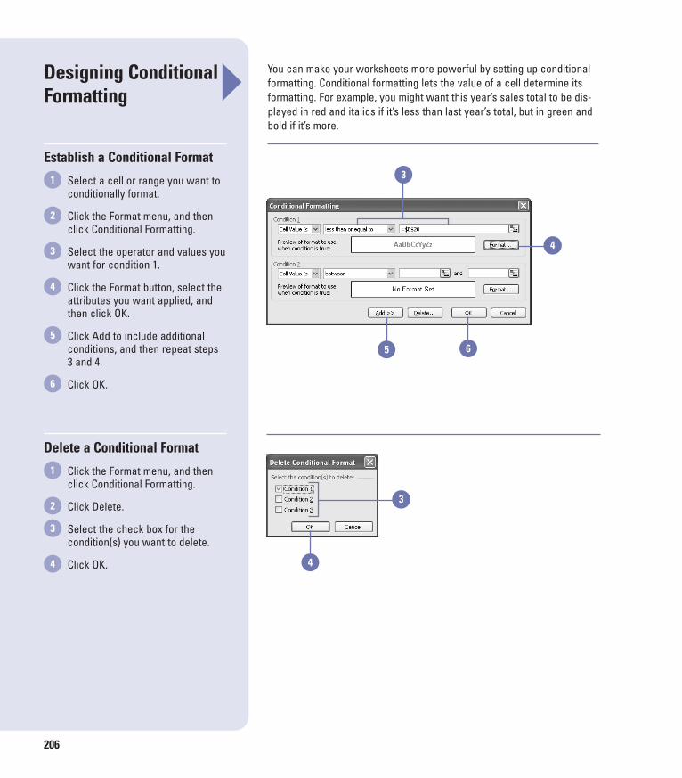
You can make your worksheets more powerful by setting up conditionalformatting. Conditional formatting lets the value of a cell determine itsformatting. For example, you might want this year’s sales total to be dis-played in red and italics if it’s less than last year’s total, but in green andbold if it’s more.

Designing ConditionalFormatting

Establish a Conditional Format

Select a cell or range you want toconditionally format.

Click the Format menu, and thenclick Conditional Formatting.

Select the operator and values youwant for condition 1.

Click the Format button, select theattributes you want applied, andthen click OK.

Click Add to include additionalconditions, and then repeat steps3 and 4.

Click OK.

Delete a Conditional Format

Click the Format menu, and thenclick Conditional Formatting.

Click Delete.

Select the check box for thecondition(s) you want to delete.

Click OK.4

3

2

1

6

5

4

3

2

1 3

4

65

4

3

C09OF.qxd 8/17/2003 11:33 PM Page 206

Designing a Worksheet with Excel 207

9

Colors and patterns added to the worksheet’s light gray grid help identifydata and streamline entering and reading data. If your data spans manycolumns and rows, color every other row light yellow to help readers fol-low the data. Or add a red dot pattern to cells with totals. Color addsbackground shading to a cell. Patterns add dots or lines to a cell in anycolor you choose. You can use the Format Cells dialog box to add colorand patterns to a worksheet. However, if you want to add color to cellsquickly, you can use the Fill Color button on the Formatting toolbar.

Adding Color andPatterns to Cells

Apply Color and Patterns

Select a cell or range to which youwant to apply colors and patterns.

Click the Format menu, and thenclick Cells.

Click the Patterns tab.

To add shading to the cell, click acolor in the palette.

To add a pattern to the cell, clickthe Pattern list arrow, and thenclick a pattern and color in thepalette.

Click OK.

Apply Color Using theFormatting Toolbar

Select a cell or range.

Click the Fill Color list arrow on theFormatting toolbar.

If necessary, click the ToolbarOptions list arrow to display thebutton.

Click a color.3

2

1

6

5

4

3

2

13

4

5 6

2

3

1

XL03S-3-1

C09OF.qxd 8/17/2003 11:33 PM Page 207

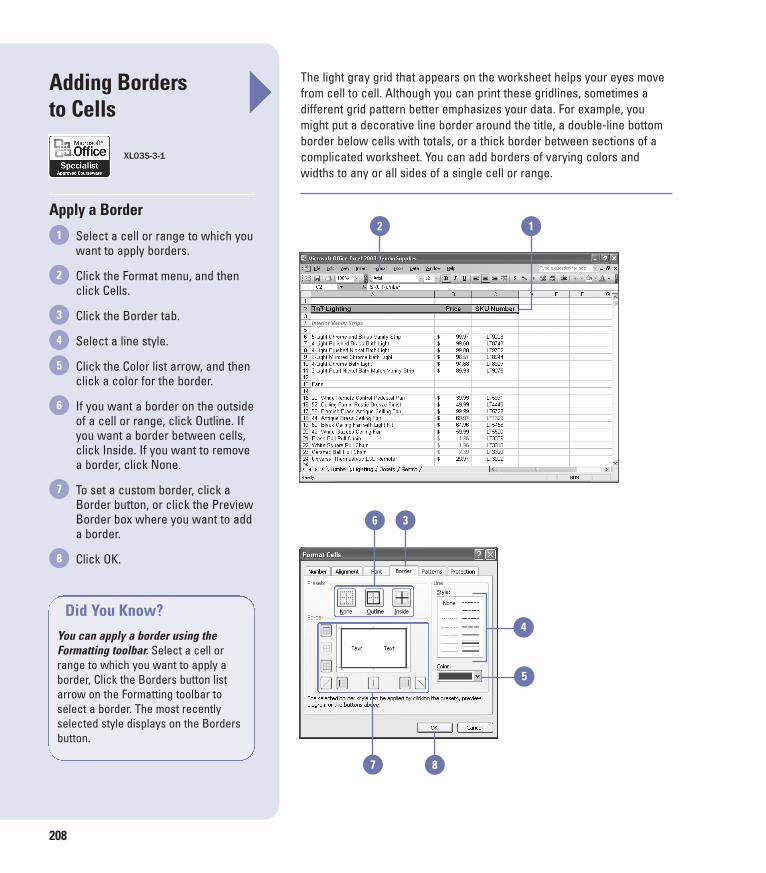
The light gray grid that appears on the worksheet helps your eyes movefrom cell to cell. Although you can print these gridlines, sometimes a different grid pattern better emphasizes your data. For example, youmight put a decorative line border around the title, a double-line bottomborder below cells with totals, or a thick border between sections of acomplicated worksheet. You can add borders of varying colors andwidths to any or all sides of a single cell or range.

208

Adding Borders to Cells

Apply a Border

Select a cell or range to which youwant to apply borders.

Click the Format menu, and thenclick Cells.

Click the Border tab.

Select a line style.

Click the Color list arrow, and thenclick a color for the border.

If you want a border on the outsideof a cell or range, click Outline. Ifyou want a border between cells,click Inside. If you want to removea border, click None.

To set a custom border, click aBorder button, or click the PreviewBorder box where you want to adda border.

Click OK.8

7

6

5

4

3

2

1

Did You Know?You can apply a border using theFormatting toolbar. Select a cell orrange to which you want to apply aborder, Click the Borders button listarrow on the Formatting toolbar toselect a border. The most recentlyselected style displays on the Bordersbutton.

1

6 3

4

5

87

2

XL03S-3-1

C09OF.qxd 8/17/2003 11:33 PM Page 208

Designing a Worksheet with Excel 209

9

Formatting worksheet data can be a lot of fun but also very intensive. Tomake formatting data more efficient, Excel includes 18 AutoFormats. AnAutoFormat includes a combination of fill colors and patterns, numericformats, font attributes, borders, and font colors that are professionallydesigned to enhance your worksheets. If you don’t select any cellsbefore choosing the AutoFormat command, Excel will “guess” whichdata should it should format.

Formatting Data with AutoFormat

Apply an AutoFormat

Select a cell or range to which youwant to apply an AutoFormat, orskip this step if you want Excel to“guess” which cells to format.

Click the Format menu, and thenclick AutoFormat.

Click an AutoFormat in the list.

Click Options.

Select one or more Formats ToApply check boxes to turn afeature on or off.

Click OK.6

5

4

3

2

1

Did You Know?You can copy cell formats with FormatPainter. Select the cell or range whoseformatting you want to copy, double-click the Format Painter button on theStandard toolbar, select the cells youwant to format, and then click theFormat Painter button.

6

4

3

5

XL03S-3-1

C09OF.qxd 8/17/2003 11:33 PM Page 209

210

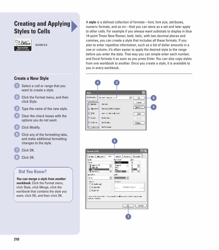
A style is a defined collection of formats—font, font size, attributes,numeric formats, and so on—that you can store as a set and later applyto other cells. For example if you always want subtotals to display in blue14-point Times New Roman, bold, italic, with two decimal places andcommas, you can create a style that includes all these formats. If youplan to enter repetitive information, such as a list of dollar amounts in arow or column, it’s often easier to apply the desired style to the rangebefore you enter the data. That way you can simple enter each number,and Excel formats it as soon as you press Enter. You can also copy stylesfrom one workbook to another. Once you create a style, it is available toyou in every workbook.

Creating and ApplyingStyles to Cells

Create a New Style

Select a cell or range that youwant to create a style.

Click the Format menu, and thenclick Style.

Type the name of the new style.

Clear the check boxes with theoptions you do not want.

Click Modify.

Click any of the formatting tabs,and make additional formattingchanges to the style.

Click OK.

Click OK.8

7

6

5

4

3

2

1

Did You Know?You can merge a style from anotherworkbook. Click the Format menu,click Style, click Merge, click theworkbook that contains the style youwant, click OK, and then click OK.

4 3

8

5

6

7

XL03S-3-2

C09OF.qxd 8/17/2003 11:33 PM Page 210

Designing a Worksheet with Excel 211

9

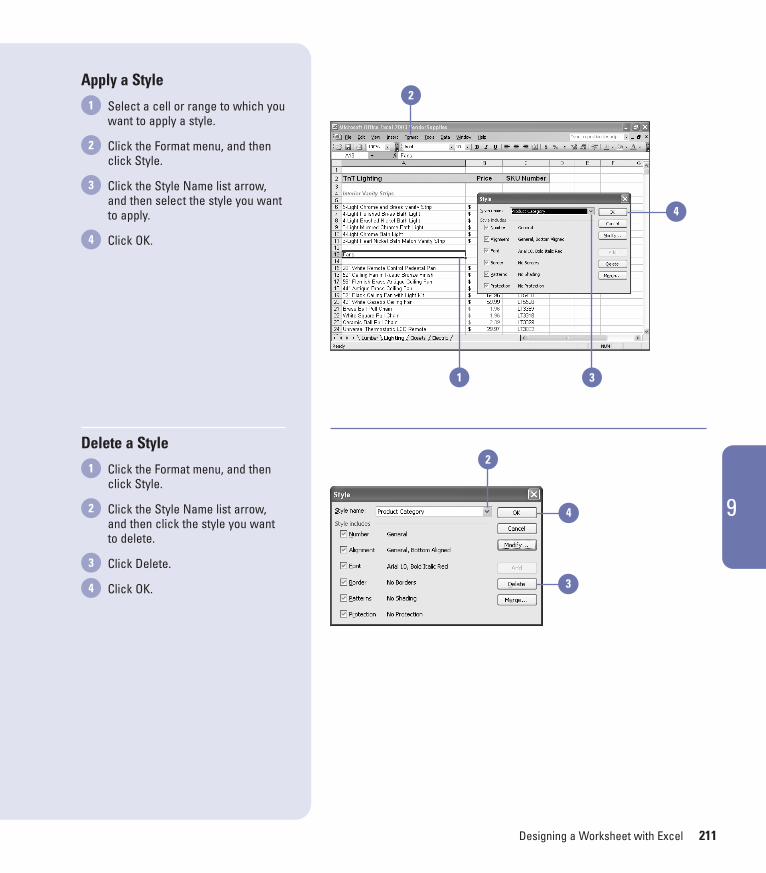
Apply a Style

Select a cell or range to which youwant to apply a style.

Click the Format menu, and thenclick Style.

Click the Style Name list arrow,and then select the style you wantto apply.

Click OK.

Delete a Style

Click the Format menu, and thenclick Style.

Click the Style Name list arrow,and then click the style you wantto delete.

Click Delete.

Click OK.4

3

2

1

4

3

2

1

4

31

2

4

3

2

C09OF.qxd 8/17/2003 11:33 PM Page 211

212

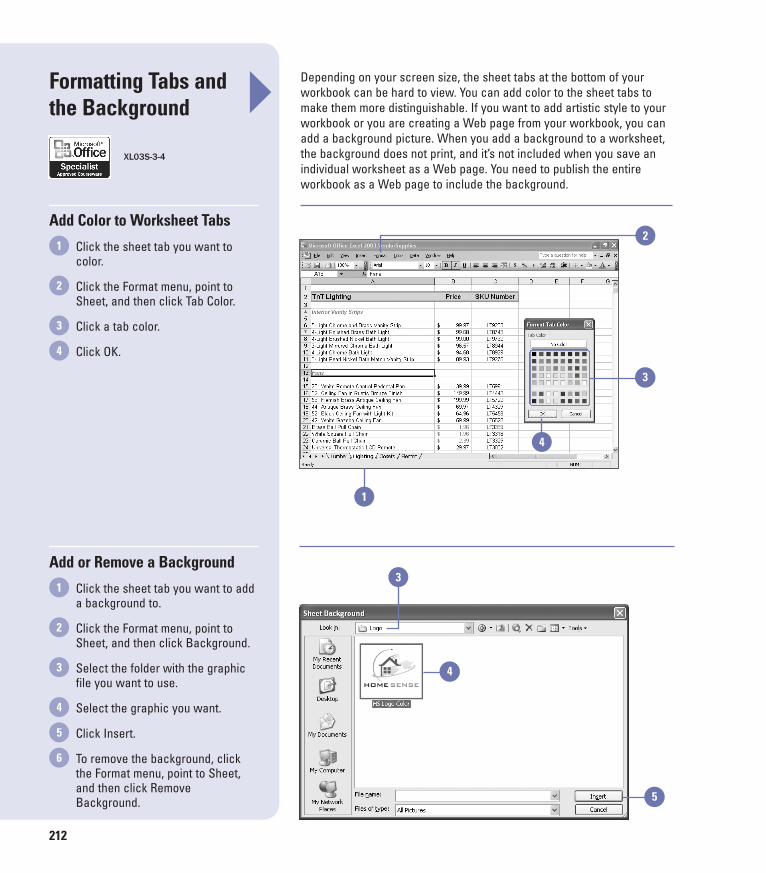
Depending on your screen size, the sheet tabs at the bottom of yourworkbook can be hard to view. You can add color to the sheet tabs tomake them more distinguishable. If you want to add artistic style to yourworkbook or you are creating a Web page from your workbook, you canadd a background picture. When you add a background to a worksheet,the background does not print, and it’s not included when you save anindividual worksheet as a Web page. You need to publish the entireworkbook as a Web page to include the background.

Formatting Tabs andthe Background

Add Color to Worksheet Tabs

Click the sheet tab you want tocolor.

Click the Format menu, point toSheet, and then click Tab Color.

Click a tab color.

Click OK.

Add or Remove a Background

Click the sheet tab you want to adda background to.

Click the Format menu, point toSheet, and then click Background.

Select the folder with the graphicfile you want to use.

Select the graphic you want.

Click Insert.

To remove the background, clickthe Format menu, point to Sheet,and then click RemoveBackground.

6

5

4

3

2

1

4

3

2

1

3

4

5

4

3

1

XL03S-3-4

2

C09OF.qxd 8/17/2003 11:33 PM Page 212

Designing a Worksheet with Excel 213

9

If you want to print a worksheet that is larger than one page, Exceldivides it into pages by inserting automatic page breaks. These pagebreaks are based on paper size, margin settings, and scaling options youset. You can change which rows or columns are printed on the page byinserting horizontal or vertical page breaks. In page break preview, youcan view the page breaks and move them by dragging them to a differentlocation on the worksheet.

Inserting Page Breaks

Insert a Page Break

To insert a horizontal page break,click the row where you want toinsert a page break.

To insert a vertical page break,click the column where you wantto insert a page break.

Click the Insert menu, and thenclick Page Break.

Preview and Move a Page Break

Click the View menu, and thenclick Page Break Preview.

Drag a page break (a thick blueline) to a new location.

When you’re done, click the Viewmenu, and then click Normal.

3

2

1

2

1

2

1

1

2

XL03S-5-5, XL03S-5-7

C09OF.qxd 8/17/2003 11:34 PM Page 213

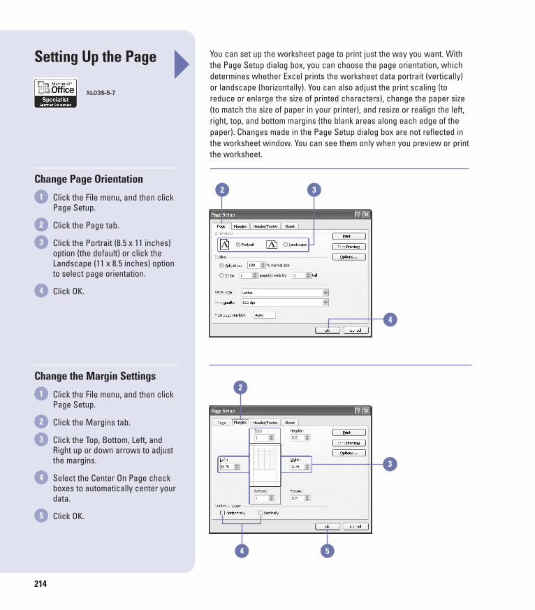
You can set up the worksheet page to print just the way you want. Withthe Page Setup dialog box, you can choose the page orientation, whichdetermines whether Excel prints the worksheet data portrait (vertically)or landscape (horizontally). You can also adjust the print scaling (toreduce or enlarge the size of printed characters), change the paper size(to match the size of paper in your printer), and resize or realign the left,right, top, and bottom margins (the blank areas along each edge of thepaper). Changes made in the Page Setup dialog box are not reflected inthe worksheet window. You can see them only when you preview or printthe worksheet.

214

Setting Up the Page

Change Page Orientation

Click the File menu, and then clickPage Setup.

Click the Page tab.

Click the Portrait (8.5 x 11 inches)option (the default) or click theLandscape (11 x 8.5 inches) optionto select page orientation.

Click OK.

Change the Margin Settings

Click the File menu, and then clickPage Setup.

Click the Margins tab.

Click the Top, Bottom, Left, andRight up or down arrows to adjustthe margins.

Select the Center On Page checkboxes to automatically center yourdata.

Click OK.5

4

3

2

1

4

3

2

12

5

2

4

3

4

3

XL03S-5-7

C09OF.qxd 8/17/2003 11:34 PM Page 214

Adding a header or footer to a workbook is a convenient way to makeyour printout easier for readers to follow. Using the Page Setup com-mand, you can add information such as page numbers, the worksheettitle, or the current date at the top and bottom of each page or section ofa worksheet or workbook. Using the Custom Header and Custom Footerbuttons, you can include information such as your computer system’sdate and time, the name of the workbook and sheet, a graphic, or othercustom information.

Designing a Worksheet with Excel 215

9

Adding Headers andFooters

Change a Header or Footer

Click the File menu, and then clickPage Setup.

Click the Header/Footer tab.

If the Header box doesn’t containthe information you want, clickCustom Header.

Type the information in the Left,Center, or Right Section text boxes,or click a button to insert built-inheader information. If you don’twant a header to appear at all,delete the text and codes in thetext boxes.

Select the text you want to format,click the Font button, make fontchanges, and then click OK. Excelwill use the default font, Arial,unless you change it.

Click OK.

If the Footer box doesn’t containthe information that you want,click Custom Footer.

Type information in the Left,Center, or Right Section text boxes,or click a button to insert the built-in footer information.

Click OK.

Click OK.10

9

8

7

6

5

4

3

2

1 6

4

2

7

3

10

5

XL03S-5-7

C09OF.qxd 8/17/2003 11:34 PM Page 215

216

At some point you’ll want to print your worksheet so you can distribute itto others or use it for other purposes. You can print all or part of anyworksheet, and you can control the appearance of many features, suchas whether gridlines are displayed, whether column letters and rownumbers are displayed, or whether to include print titles, columns androws that are repeated on each page. If you have already set a printarea, it will appear in the Print Area box on the Sheet tab of the PageSetup dialog box. You don’t need to re-select it.

CustomizingWorksheet Printing

Print Part of a Worksheet

Click the File menu, and then clickPage Setup.

Click the Sheet tab.

Click in the Print Area box, andthen type the range you want toprint. Or click the Collapse Dialogbutton, select the cells you want toprint, and then click the ExpandDialog button to restore the dialogbox.

Click OK.

Print Row and Column Titles onEach Page

Click the File menu, and then clickPage Setup.

Click the Sheet tab.

Enter the number of the row or theletter of the column that containsthe titles. Or click the CollapseDialog button, select the row orcolumn with the mouse, and thenclick the Expand Dialog button torestore the dialog box.

Click OK.4

3

2

1

4

3

2

1

4

3 2

4

32

Collapse Dialog button

XL03S-5-7, XL03S-5-8

Collapse Dialogbutton

C09OF.qxd 8/17/2003 11:34 PM Page 216

Designing a Worksheet with Excel 217

9

Print Gridlines, Column Letters,and Row Numbers

Click the File menu, and then clickPage Setup.

Click the Sheet tab.

Select the Gridlines check box.

Select the Row And ColumnHeadings check box.

Click OK.

Fit Your Worksheet on a SpecificNumber of Pages

Click the File menu, and then clickPage Setup.

Click the Page tab.

Select a scaling option.

◆ Click the Adjust To option toscale the worksheet using apercentage.

◆ Click the Fit To option to force aworksheet to be printed on aspecific number of pages.

Click OK.4

3

2

1

5

4

3

2

1

2

4

53

2

3

4

C09OF.qxd 8/17/2003 11:34 PM Page 217

218

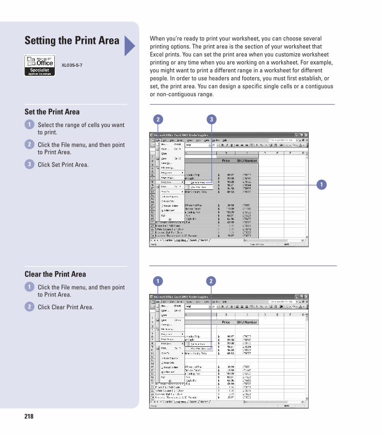
When you’re ready to print your worksheet, you can choose severalprinting options. The print area is the section of your worksheet thatExcel prints. You can set the print area when you customize worksheetprinting or any time when you are working on a worksheet. For example,you might want to print a different range in a worksheet for differentpeople. In order to use headers and footers, you must first establish, orset, the print area. You can design a specific single cells or a contiguousor non-contiguous range.

Setting the Print Area

Set the Print Area

Select the range of cells you wantto print.

Click the File menu, and then pointto Print Area.

Click Set Print Area.

Clear the Print Area

Click the File menu, and then pointto Print Area.

Click Clear Print Area.2

1

3

2

12 3

1

1 2

XL03S-5-7

C09OF.qxd 8/17/2003 11:34 PM Page 218

Designing a Worksheet with Excel 219

9

Before printing, you should verify that the page looks the way you want.You save time, money, and paper by avoiding duplicate printing. PrintPreview shows you the exact placement of your data on each printedpage. You can view all or part of your worksheet as it will appear whenyou print it. The Print Preview toolbar makes it easy to zoom in and out toview data more comfortably, set margins and other page options, pre-view page breaks, and print.

Previewing aWorksheet

Preview a Worksheet

Click the Print Preview button onthe Standard toolbar, or click theFile menu, and then click PrintPreview.

Click the Zoom button on the PrintPreview toolbar, or position theZoom pointer anywhere on theworksheet and click it to enlarge aspecific area of the page.

If you do not want to print fromPrint Preview, click the Closebutton to return to the worksheet.

If you want to print from PrintPreview, click the Print button onthe Print Preview toolbar.

Click OK.5

4

3

2

1

Did You Know?You can preview your work from thePrint dialog box. In the Print dialogbox, click Preview. After previewingyou can click the Print button on thePrint Preview toolbar to print the work-sheet or click the Close button toreturn to your worksheet.

1

342

XL03S-5-5

C09OF.qxd 8/17/2003 11:34 PM Page 219

220

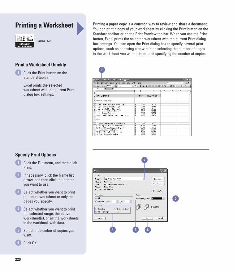
Printing a paper copy is a common way to review and share a document.You can print a copy of your worksheet by clicking the Print button on theStandard toolbar or on the Print Preview toolbar. When you use the Printbutton, Excel prints the selected worksheet with the current Print dialogbox settings. You can open the Print dialog box to specify several printoptions, such as choosing a new printer, selecting the number of pagesin the worksheet you want printed, and specifying the number of copies.

Printing a Worksheet

Print a Worksheet Quickly

Click the Print button on theStandard toolbar.

Excel prints the selectedworksheet with the current Printdialog box settings.

Specify Print Options

Click the File menu, and then clickPrint.

If necessary, click the Name listarrow, and then click the printeryou want to use.

Select whether you want to printthe entire worksheet or only thepages you specify.

Select whether you want to printthe selected range, the activeworksheet(s), or all the worksheetsin the workbook with data.

Select the number of copies youwant.

Click OK.6

5

4

3

2

1

11

2

5

634

XL03S-5-8

C09OF.qxd 8/17/2003 11:34 PM Page 220