Attribution-NonCommercial-ShareAlike 3.0 Unported (CC BY-NC-SA 3.0)

This is a human-readable summary of the Legal Code (the full license).

Disclaimer

You are free:

to Share — to copy, distribute and transmit the work

to Remix — to adapt the work

Under the following conditions:

Attribution — You must attribute the work in the manner specified by the author or

licensor (but not in any way that suggests that they endorse you or your use of the

work).

Noncommercial — You may not use this work for commercial purposes.

Share Alike — If you alter, transform, or build upon this work, you may distribute the

resulting work only under the same or similar license to this one.

With the understanding that:

Waiver — Any of the above conditions can be waived if you get permission from the

copyright holder.

Public Domain — Where the work or any of its elements is in the public domain under

applicable law, that status is in no way affected by the license.

Other Rights — In no way are any of the following rights affected by the license:

Your fair dealing or fair use rights, or other applicable copyright exceptions and

limitations;

The author's moral rights;

Rights other persons may have either in the work itself or in how the work is

used, such aspublicity or privacy rights.

Notice — For any reuse or distribution, you must make clear to others the license terms

of this work. The best way to do this is with a link to this web page.

This page is available in the following languages: Castellano Castellano

(España) Català Deutsch English Esperanto français hrvatski Indonesia Italiano Magyar Nederlands Norsk

polski Português Português (BR) Suomeksi svenska íslenska Ελληνικά русский українська 中文 華語 (台

灣) 한국어

Biomedical Engineering and Biophysics

September 2013 2 de 10

Designing and evaluating a Steady State Visually Evoked Potentials based

Brain Computer Interface system

Author: Mauro Rafael Oliveira Sansana

Abstract: “In this report I describe the Steady State Visually Evoked Potentials based Brain

Computer Interface system that I built during my summer internship in the University of

Twente, using the Emotiv© EPOC headset, the Psychophysics Toolbox extension for Matlab

®

and the Simulink®/Matlab

® environment. I then test and evaluate the system, using data recorded

from a subject and signal analysis techniques, coming to the conclusion that, although there is

still room for improvements, the system can clearly present the frequency at which the stimulus

is being delivered through the Psychophysics Toolbox.”

Resumo: “Neste relatório descrevo o sistema Interface Cérebro Computador baseado em Steady

State Visually Evoked Potentials construído por mim durante o meu estágio de verão na

Universidade de Twente, utilizando o conjunto Emotiv© EPOC, a caixa de ferramentas

Psychophysics para o Matlab® e o ambiente Simulink

®/Matlab

®. Depois testo e avalio o sistema,

utilizando dados recolhidos de um sujeito e técnicas de análise de sinal, chegando à conclusão

de que, apesar de ainda haver espaço para melhoria, o sistema consegue claramente apresentar a

frequência de estimulação que é entregue através da caixa de ferramentas Psychophysics.”

1. Introduction

“The possibility that signals recorded

from the brain might be used for

communication and control has engaged

popular and scientific interest for many

decades. However, it is only in the last 25

years that sustained research has begun

(…)” [1]. The ever-growing understanding

of the central nervous system (CNS) that

has emerged from animal and human

research over the past 50 years, the

appearance of powerful inexpensive

computer hardware and software that can

support complex high-speed analyses of

brain activity and the recognition of the

needs and abilities of people disabled by

disorders such as stroke, spinal cord injury,

multiple sclerosis and muscular

dystrophies, were the main catalysts for the

surge in scientific interest and activity in

the field of Brain Computer Interfaces

(BCIs), in the past 5-10 years [1].

1.1. Brain-Computer

Interface

A BCI is a system of communication in

which the messages or commands that an

individual sends to the external world do

not pass through the brain’s normal output

pathways of peripheral nerves and muscles,

but instead are encoded in

electroencephalography (EEG) activity (for

example, in a EEG-based BCI). This allows

for the user to have an alternative method

for acting on their surroundings [2].

Designing and evaluating a Steady State Visually Evoked Potentials based Brain Computer

Interface system

1 An EEG evoked potential (EP) is a distinctive pattern of positive and negative voltage deflections that is

time correlated with a specific sensory stimulus or event [1].

3 de 10

BCIs fall into two classes: dependent

and independent. An independent BCI, as

the name indicates, does not depend in any

way on the brain’s normal output pathways

(peripheral nerves and muscles), and so

activity in these pathways is not needed to

generate brain activity (e. g. EEG) that

carries the message. A dependent BCI, on

the other hand, does not use the brain’s

normal output to carry the message, but

instead stimulates activity in these

pathways to generate brain activity (e. g.

EEG) that does carry it [2]. An example of

a dependent BCI is an SSVEP-based BCI

(see section Background).

2. Motivation

I’m a gamer for a long time, and I’ve

always been fascinated with neurosciences.

The use of a BCI system as input for a

gaming system opens new opportunities

and interactions in game and also allows for

gamers with disabilities that in any way

hinders them to play games by the normal

inputs, like keyboard, mouse or gamepad,

with an opportunity to experience new

sensations.

My final goal is to design a BCI system

that allows for the control of a computer

based game with a specially designed

interface. This system should use an EEG

device that is available commercially, and

therefore available for every common

player.

3. Background

3.1. Steady-State Visually

Evoked Potentials

There are a few options for building a

BCI. The most common ones are those that

use: P300 event-related potentials;

Sensorimotor Rhythms; Steady-State

Visually Evoked Potentials (SSVEPs) and

Brain Metabolic Signals.

Although P300 and Sensorimotor

Rhythms are the most used EEG features

for BCIs, my work focuses on the use of

SSVEPs. A Visually Evoked Potential

(VEP) is a potential evoked1 by a sudden

visual stimulus, such as a light flash, the

appearance of an image, or an abrupt

change in colour or pattern. These

potentials are generated in or near the

primary visual cortex and thus are more

prominent over occipital scalp areas.

Steady-State VEPs (SSVEPs) are stable

oscillations in voltage that are elicited by

rapid repetitive stimulation such as a strobe

light, a LED, or a pattern-reversing

checkerbox presented on a monitor (see

Fig. 1) [1,3].

There are three main theories that

explain the propagation of SSVEPs in the

brain. The first theory considers that

SSVEPs originate in the primary Visual

Cortex and propagate by the combined

activity of locally and broadly distributed

sources [3,4].

Fig. 1 Examples of stimuli used to elicit SSVEP

responses. (a)Flickering light mounted on goggles

(usually LCD or LED goggles); (b) light-emitting diode,

producing flickering light; and (c) flickering images on

a computer screen: (c0) combination of images, (c1)

simple square, (c2) checkerboard, (c3) image, (c4)

Gaussian field, (c5) sinusoidally modulated square, (c6)

rotating or moving stimuli, and (c7) moving vertical or

horizontal gratings [3].

Designing and evaluating a Steady State Visually Evoked Potentials based Brain Computer

Interface system

4 de 10

The second theory considers that

SSVEPs are generated by a finite number of

electrical dipoles that are activated

sequentially in time, starting with a dipole

located in the Striate Cortex [3,5]. The last

theory considers that VEPs are generated in

the primary visual cortex, and propagate to

other brain areas through cortical and

standing wave models [3,6,7].

Despite this lack of consensus among

researchers, in general the different studies

point to a major source of SSVEPs located

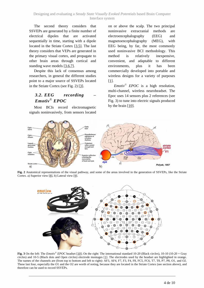
in the Striate Cortex (see Fig. 2) [3].

3.2. EEG recording –

Emotiv©

EPOC

Most BCIs record electromagnetic

signals noninvasively, from sensors located

on or above the scalp. The two principal

noninvasive extracranial methods are

electroencephalography (EEG) and

magnetoencephalography (MEG), with

EEG being, by far, the most commonly

used noninvasive BCI methodology. This

method is relatively inexpensive,

convenient, and adaptable to different

environments, plus it has been

commercially developed into portable and

wireless designs for a variety of purposes

[1].

Emotiv© EPOC is a high resolution,

multi-channel, wireless neuroheadset. The

Epoc uses 14 sensors plus 2 references (see

Fig. 3) to tune into electric signals produced

by the brain [10].

Fig. 2 Anatomical representations of the visual pathway, and some of the areas involved in the generation of SSVEPs, like the Striate

Cortex. a) Superior view [8], b) Lateral view [9].

Fig. 3 On the left: The Emotiv© EPOC headset [10]; On the right: The international standard 10-20 (Black circles), 10-10 (10-20 + Gray

circles) and 10-5 (Black dots and Open circles) electrode montages [1]. The electrodes used by the headset are highlighted in orange.

The names of the channels are (from top to bottom and left to right): AF3, AF4, F7, F3, F4, F8, FC5, FC6, T7, T8, P7, P8, O1, and O2.

These last four, especially the O1 and the O2 are worth of noting, because they are located in the Striate Cortex (see section above), and

therefore can be used to record SSVEPs.

Designing and evaluating a Steady State Visually Evoked Potentials based Brain Computer

Interface system

2 The Matlab

® code for the system is available for consulting in the annexes section of this document

(Erro! A origem da referência não foi encontrada.).

5 de 10

This system is portable and wireless,

does not require extensive head preparation

like other systems (it only requires some

contact lens solution, to wet the electrodes),

and is relatively easy for someone without

any training, to use in the field.

Furthermore, together with the Epoc

Simulink EEG Importer software

(developed by MathWorks®), it is possible

to store the EEG data, such as the recording

channels and the values detected in each

channel, in a Simulink®/Matlab

®

environment, for further analysis and

processing.

3.3. Stimuli delivery system

– Psychtoolbox

In order to build a visual stimuli delivery

system, I choose the Psychophysics

Toolbox extension for Matlab® [11,12,13].

This toolbox is a free set of Matlab® and

GNU/Octave® functions for vision research.

It was designed to make it easy to

synthesize and show accurately controlled

visual stimuli [14].

4. The Design

Given that I only had two months to

design and test a BCI system, I knew from

the start that I would not be able to make a

fully functional system so, having Fig. 4 as

an example I have designed an SSVEP

based BCI system to test the Emotiv©

EPOC headset and to observe the existence

of SSVEPs in the EEG data that I would

acquire.

4.1. Global design

After some work reading and learning, I

designed a simple system that would allow

me to observe the SSVEPs in the user EEG

data (see Fig. 5).

4.2. Overall building blocks

4.2.1. The Stimuli System

To design the stimuli system I chose the

Psychophysics Toolbox extension for

Matlab®, that allows me to easily deliver a

stimulus through Matlab®. As for the type

of stimulus itself, I chose to deliver a

sinusoidally modulated rectangle (see Fig.

1c5) on a black background, approximately

150 pixels away from each edge of the

screen2. Using a sinusoid wave (see Eq. 1)

with a given frequency, I was able to

modulate the rectangle RGBA (Red, Green,

Blue, Alpha) color values, more precisely

the Alpha value (transparency).

⁄ Eq. 1 Sinusoid wave equation.

Fig. 4 Example of a typical SSVEP-based BCI. A screen (usually

a computer screen) displays the visual stimulus to the user, in this

case a checkerboard type stimulus. The electrodes on the user’s

scalp then record the EEG signal. Next, software processes the

signals and recognizes the SSVEPs, translating them into

commands that, in this case, are used to change the stimuli

(feedback). Image adapted from [15].

Stimuli System

a)

User EEG Recording System

b) c) Signal Process and

Visual Analysis

Fig. 5 A basic and practical SSVEP-based BCI system. a) Visual Stimuli; b) Visual Pathways and SSVEPs sources; c) Software.

Designing and evaluating a Steady State Visually Evoked Potentials based Brain Computer

Interface system

3 The Matlab® code for the system is available for consulting in the annexes section of this document

(Erro! A origem da referência não foi encontrada.). 6 de 10

The result is a flickering rectangle on a

black background, gradually changing from

pure white to black, with a predetermined

frequency (see Fig. 7 and watch the

YouTube video at [16], for an example of

the system).

Next, I designed a timeline for the

experiment, so that I had different types of

data to analyse. Reading through some

articles, I decided to go with the 15Hz

frequency for my system (see Fig. 6), for

the same reason that I had decided to go for

a fullscreen single frequency flickering

rectangle, because I wanted to clearly see

the effects (SSVEPs) of the visual stimuli

on the EEG signals. After a few attempts

and experiments, I decided to go with a

basic timeline for the system: starting with

a black background the system should

present the user with 10 seconds of “idling

time”, in which the screen should remain

black, followed by 20 seconds of

“flickering time”, in which the rectangle

will appear and flicker, followed by another

10 seconds of “idling time”, with this cycle

repeating itself for 120 seconds, 2 minutes

(see Fig. 8).3

4.2.2. The EEG recording system

Using the Simulink® environment,

together with the Epoc Simulink EEG

Importer software (developed by

MathWorks®), I was able to visualize the

EEG data from the Emotiv© EPOC headset

in real time and also record that data to a

file, all this from within the Matlab®/

Simulink® environment.

This software comes with a Signal

Server application, that is responsible for

making the connection between the

Emotiv© EPOC headset and the Simulink

®

environment, and it also comes with a pre-

made model for the Simulink®, that allows

the user to easily construct a system, taking

the pre-made as a starting point. My final

model can be seen in Fig. 9.

Fig. 7 Example of the stimuli delivery system. The

rectangle is perfectly centred with 150 pixels (~4cm)

away from each edge of the screen. In a 1980x1080

screen resolution, this means that the rectangle is,

approximately, 47 cm long and 25 cm tall. The whole

system can be seen in [16].

Fig. 6 A plot that shows the average SSVEP amplitude in the occipital area

of the brain, for different flickering frequencies.

Sti

mulu

s P

rese

nce

Time (s)

1st

Trial

2nd

Trial

3rd

Trial

4th

Trial

5th

Trial

6th

Trial

7th

Trial

8th

Trial

9th

Trial

10th

Trial

11th

Trial

12th

Trial

0 10 30 40 60 70 90 100 120 0

1

Fig. 8 The timeline for the experiment. The system starts with a black screen, which corresponds to a Stimulus Presence value of 0 or “idling

time” and, therefore, the Stimulus value of 1 corresponds to the “flickering time”. Each trial is 10 seconds long.

Designing and evaluating a Steady State Visually Evoked Potentials based Brain Computer

Interface system

4 Harmonic frequencies are equally spaced by the width of the fundamental frequency and can be found

by repeatedly adding that frequency. [17]

7 de 10

This model is divided into two sub-

systems: one that receives the EEG from

the Signal Server (the

cmex_EmotivEpocEEG block on Fig. 9a)

and saves it to a file (the To_file_1 block on

Fig. 9a) as a time series matrix; and the

other sub-system that calls a Matlab®

function4 when the system starts. This

second sub-system stores the computer OS

time in seconds in a vector, which is used,

together with a similar function nested

inside the stimuli system, to correlate both

systems to the same time period.

4.2.3. The signal process and visual

analysis system

SSVEPs may be analysed by

conventional averaging methods or by

frequency analysis (e.g. the Fast Fourier

Transform algorithm). Frequency analysis

normally reveals a peak at the frequency of

stimulation (in this case 15Hz), as well as

peaks at higher harmonic frequencies, for

example, the 1st harmonic frequency for

15Hz (which is the fundamental frequency)

is 30Hz4 [1,17].

So, by taking the three files generated

from the systems above (two files from the

recording system and one from the stimuli),

I wrote a script in Matlab® that will first

load the files onto the workspace, then it

will take the info in the EEG data file and

save each channel to a different vector.

This process is made easier by the fact

that the file is in time series format, with a

very well-defined sampling frequency of

128 (Emotiv© EPOC headset), so each

channel is perfectly time correlated inside

the time series, and can be extracted into

individual vectors using Matlab® functions.

As the recording system and the stimuli

system are not initiated at the same time

(the recording system needs to be initiated

earlier), it is necessary to find the time at

which the stimuli system began, related to

the beginning of the recording. And that is

where the files with the computer OS time

come to help. One of the files has the time,

in seconds, that the computer OS had at the

beginning of the recording, and the other

file has the same info, but at the beginning

of the stimulus.

So by subtracting those values I get

another value in seconds that gives me the

time elapsed between the start of the

recording and the start of the stimuli, and

by searching for that value on the time

vector of the time series, I can know which

index corresponds to that moment, with that

index being valid for all the channels.

Fig. 9 Simulink® environment model for the recording system. a) sub-system that receives the data from the Signal

Server; b) sub-system that saves the computer OS time in seconds to a file, when the model is started.

From Signal Server

Designing and evaluating a Steady State Visually Evoked Potentials based Brain Computer

Interface system

5 The Matlab

® code for the system is available for consulting in the annexes section of this document

(Erro! A origem da referência não foi encontrada.). Note that the code is written to only handle the O2

channel, but can be modified to handle any channel from the data file. 6 The frequency scale can be represented as a full circle where can be considered as the positive

frequencies and as the negative ones [18]. 7 The Nyquist frequency is half of the sampling rate of a discrete signal processing system [19].

8 de 10

Now I needed to split the 120 seconds

length data into smaller segments, called

trials. I chose to split it into 10 seconds

trials (which gives me 12 segments), just

because that way I would have the “idling

time” in a single trial and the “flickering

time” in two consecutive trials, which

facilitates the splitting process. So, after

this process, I would have each channel

vector split into two matrices each, one

matrix for the “idling time” data and

another matrix for the “flickering time”,

with each row of the matrix corresponding

to a different trial.5

The values of amplitude from the EEG

channels are very high, and have a high

mean value (see Fig. 10 in the section

Evaluation of the design for a more visual

representation), which can cause some

problems for the FFT algorithm. To

overcome this I used Matlab® functions,

such as: the mean function, which returns

the mean values of the elements along the

required dimension of a matrix, and the

repmat function, which creates a large

matrix consisting of a ”user defined size”

tiling of copies of another matrix. These

functions allowed me to offset the values

from the EEG channels to much lower

values and centered on the origin (the mean

of the values is now zero).

After these pre-processing steps, the

data is now ready to be processed with the

FFT algorithm. The Matlab® functions fft(x)

and ifft(X) implement the transform and

inverse transform pair given for vectors of

length N by Eq. 2:

∑

⁄ ∑

where

⁄ is the Nth root of unity.

Eq. 2 The FFT algorithm equations. As seen in

the Matlab® help browser.

In resume, the fft(x) function returns the

discrete Fourier transform (DFT) of vector

x, computed with a fast Fourier transform

(FFT) algorithm. If x is a matrix, this

function can be modified to operate on the

desired dimension which, on my case, is the

row dimension. So the next step is to apply

this function to each row of both of the

matrices created in the splitting process

described above.

This step creates a new matrix filed with

the frequency data of the trials. But this

data needs to be processed even further. So

the next step is to calculate the power in the

frequency spectrum. This is done by

multiplying each element of the matrices

created in the last step, by their complex

conjugate, and divide the result by the

length of the trial in samples (in this case is

1280 samples), which creates the power

spectrum matrices, represented in mV2 (see

Eq. 3).

Eq. 3 Example of a Matlab® script that illustrates

the steps to calculate the power spectrum values.

Note that conj(Y) is a Matlab® function that returns

the complex conjugate of the elements of Y, as seen

in the Matlab® help browser.

The last step before the power spectrum

matrices are ready to be plotted is to

transform the indexes in the matrices into

frequency values. These indexes correspond

to something called the bin, or spectrum

sample. As the power spectrum that

resulted from the real and imaginary

coefficients (after the FFT algorithm) is

even6, the part reflecting the negative

frequencies is identical to the part

containing positive frequencies, and

therefore it is common practice to depict

only the first half of the spectrum, up to the

Nyquist frequency7, which in this case is

64Hz.

Designing and evaluating a Steady State Visually Evoked Potentials based Brain Computer

Interface system

8 Note that each step described in this section was built using guidelines from [19].

9 de 10

Having that in mind I constructed a

frequency vector that as the same length of

the power spectrum matrices and so can

correlate the values from these matrices

with their correspondent frequencies.8

5. Evaluation of the design

After a few attempts at using my own

data to test my system I realised that the

system didn’t work with me, probably

because of my long hair. So I asked for a

volunteer to be my test subject and the

system worked perfectly with his data. The

data presented in this section is the result of

the processing of his data through the

system that I built.

Fig. 10 is a representation of some of the

EEG data recorded from the Emotiv© EPOC

headset. In the plot there are some clearly

visible noisy peaks in the P8 channel,

probably caused by a head movement or

loss of contact from the Emotiv© EPOC

headset electrodes, and therefore it is not a

reliable channel for the next phases. Apart

from that, there are two things worth of

noticing: first the values of amplitude are

not centred on the origin of the Y-axis and

second the length of the data is longer than

120 seconds (the stimuli system duration).

Both of these unique characteristics were

accounted for in the designing of the

systems, as I’ve mentioned before.

Just to make this report shorter and

pleasant to read, I decided to show only

some of the results from the O2 channel,

from now on. But bear in mind that the

results are similar for the other channels.

In Fig. 11 it’s visible the effect of the

Offset stage, before the use of the FFT

algorithm.

Fig. 10 Plot representation of the raw EEG values from four of the Emotiv© EPOC headset channels (O1, O2, P7 and P8).

Fig. 11 Plot of the an example of the O2 channel values that result

from the Offset pre-processing phase, between 40 and 50 seconds

after the beginning of the stimuli system.

Designing and evaluating a Steady State Visually Evoked Potentials based Brain Computer

Interface system

9 Please note that the Power values are presented in the Y axis of the plots, and that all the four plots are

presented with different scales.

10 de 10

Fig. 12 is a visual representation of the

power spectrum values in two separate

trials, during the “idling time”. It’s clearly

visible that all frequencies have high Power

values, compared to the other frequencies,

so there isn’t a “dominant frequency”.

Finally, Fig. 13 is a visual representation

of the power spectrum values in two

separate trials, during the “flickering time”.

In these plots it is clearly visible the

presence of a high power peak around

15Hz.

It’s also worth of noticing that the Power

values in the plots from the “flickering

time” (Fig. 13) are higher than those

belonging to the “idling time”9. The highest

peak from Fig. 12 is roughly 75% lower

than the highest peak from Fig. 13.

Fig. 12 Plots of two of the Power spectrum matrices from the O2

channel data, between the frequencies of 5Hz and 30Hz. Fig. 13 Plots of two of the Power spectrum matrices from the O2 channel

data, between the frequencies of 5Hz and 30Hz.

Designing and evaluating a Steady State Visually Evoked Potentials based Brain Computer

Interface system

11 de 10

6. Discussion, Conclusions

& Future Look

The evaluation of the design showed

that the system can deliver the stimuli

correctly, receive the recorded data from a

subject, process it and clearly present the

power spectrum plots, in which can be seen

the distinction between the trials belonging

to the “idling time” and to the “flickering

time”.

Although I decided to omit some of the

plots from the O2 channel and the plots

from all the other channels, due to logistic

reasons and because this channel was the

channel that presented the cleanest power

spectrum plots, I analysed them and the

results were very similar to the ones

present.

In conclusion, the designed system

worked as intended.

My long time goal, as stated in the

Motivation section, was to build a BCI

system to work with a computer based

game with a specially designed interface.

Due to my lack of skills and shortage of

time, I wasn’t able to design the whole

system, from the game itself to a fully

functional BCI system.

The next steps towards that goal should

be to first finish the signal processing

system, so that it can label each trial based

on the values from the power spectrum

matrices. One of the ways to do that could

be by using linear regression on the values

from the 15Hz frequency and the 30Hz

frequency (1st harmonic frequency). After

the labelling system works as intended, one

of the last steps should be to build a

feedback system, using the Psychophysics

Toolbox extension for Matlab®, like a maze

game with flickering squares for direction

changes, for example.

Acknowledgements

First of all I want to thank my girlfriend,

Ânia Sousa, which convinced me to make

an international internship, and if it wasn’t

for her I wouldn’t had done this work, that I

enjoyed so much.

Secondly I want to thank Prof. Mannes

Poel, from the University of Twente

(Enschede, Netherlands) Human Media

Interaction group, for having agreed to

receive me during the summer, and for all

the patience he had with me, during the

time I was in the University.

I also want to leave a special thanks to

Mariana Branco, from Instituto Superior

Técnico (Lisbon, Portugal), for giving me

some ideas for my project and for letting

me participate in her project and try it; to

Prof. Ducla Soares for “awakening” my

curiosity in Neurosciences and to Prof.

Hugo Ferreira for being the first to

introduce me to the BCI world.

Finally I want to thank Prof. Lynn

Packwood, also from the University of

Twente, for having the patience to review

my report and correct my English.

“How can a three-pound mass of

jelly that you can hold in your

palm imagine angels, contemplate

the meaning of infinity, and even

question its own place in the

cosmos? (...)”

- V.S. Ramachandran, The Tell-Tale

Brain: A Neuroscientist's Quest for

What Makes Us Human

Designing and evaluating a Steady State Visually Evoked Potentials based Brain Computer

Interface system

I

References

1) [edited by] Wolpaw, Jonathan R. &

Wolpaw, Elizabeth W. “Brain

Computer Interfaces – Principles

and Practice”. Oxford University

Press, 2012;

2) Wolpaw, Jonathan R. et al. “Brain-

computer interfaces for

communication and control”. Clin.

Neurophysiol. vol.113, no. 2, pp.

767-791, June 2002;

3) Vialatte, François-Benoît et al.

“Steady-state visually evoked

potentials: Focus on essential

paradigms and future

perspectives”. Progress in

Neurobiology vol.90, no. 4, , pp.

418–438, April 2010;

4) Srinivasan et al. “Steady-state

visual evoked potentials:

distributed local sources and wave-

like dynamics are sensitive to

flicker frequency”. Brain Topogr.

vol.18, no. 3, pp. 167–187, 2006;

5) Di Russo et al. “Spatiotemporal

analysis of the cortical sources of

the steady-state visual evoked

potential”. Hum. Brain Mapp.

vol.28, no. 4, pp. 323–334, 2007;

6) Burkitt et al. “Steady-state visual

evoked potentials and travelling

waves”. Clin. Neurophysiol.

vol.111, no. 2, pp. 246–258, 2000;

7) Silberstein, R.B. “Steady-state

visually evoked potentials, brain

resonances, and cognitive

processes”. In: Nunez, P.L. (Ed.),

Neocortical Dynamics and Human

EEG Rhythms. Oxford University

Press, Oxford, pp. 272–303, 1995;

8) Dale Purves et al. “Neuroscience”.

5th edition, Sinauer Associates, Inc,

2012;

9) Web Image: [HTML];

10) Emotiv Website: [HTML];

11) Brainard, D. H. “The

Psychophysics Toolbox”. Spatial

Vision vol.10, pp. 433-436, 1997

[PDF];

12) Pelli, D. G. “The VideoToolbox

software for visual psychophysics:

Transforming numbers into

movies”. Spatial Vision vol.10, pp.

437-442, 1997 [PDF] [HTML];

13) Kleiner M, Brainard D, Pelli D.

"What's new in Psychtoolbox-3?”.

Perception 36 ECVP Abstract

Supplement, 2007 [HTML];

14) Psychtoolbox Website: [HTML];

15) Web Image: [HTML];

16) YouTube video: [HTML];

17) Wikipedia search: [HTML];

18) Drongelen, Wim Van. “Signal

processing for neuroscientists: An

introduction to the analysis of

physiological signals”. Elsevier,

2007;

19) Wikipedia search: [HTML].

Designing and evaluating a Steady State Visually Evoked Potentials based Brain Computer

Interface system

II

Annexes

For information, contact the author: sonnekonige[at]gmail.com, thanks.