Page 1
Designing Productive Assembly System Configurations Based on
Hierarchical Subassembly Decomposition
with Application to Automotive Battery Packs
by
Sha Li
A dissertation submitted in partial fulfillment
of the requirements for the degree of
Doctor of Philosophy
(Mechanical Engineering)
in The University of Michigan
2012
Doctoral Committee
Professor S Jack Hu Chair
Professor Jionghua Jin
Professor Panos Y Papalambros
Assistant Research Scientist Hui Wang
Jeffrey Abell General Motors Co
copy Sha Li 2012
ii
DEDICATION
To my family
iii
ACKNOWLEDGEMENTS
I would like to first thank my advisor Professor Jack Hu for recruiting and
mentoring me Without his encouragement and discovery I would not be able to apply
for and get admitted to the world class engineering school at the University of Michigan
Without his guidance and support I would not be able to accomplish what I have done in
graduate school His great vision vast knowledge invaluable inspiration and inquisitive
questions have given me wisdom and strength to continue my research His enormous
patience and persistent confidence in me supported me when my progress stalled Going
through graduate school with him as an advisor have been a valuable process which will
benefit me for a long time to come
I would also like to thank all my committee members for all their help In
particular Professor Panos Y Papalambros and Professor Judy Jin for their insights and
suggestions on my dissertation for being a great help throughout my faculty search
application process Dr Hui Wang for not only providing guidance to me on the big
picture but also working with me in detailed programming side by side Dr Jeffrey Abell
for giving me opportunities to work as an intern three times at General Motors which
help me gain many industry experiences and conduct application-based research In
addition I want to thank my mentor at General Motors Yhu-Tin Lin for providing me
his industrial insights experience and expertise to my research
iv
I would like to thank all the group members in the Hu lab past and present They
have made my graduate school life so much more enjoyable I want to thank them all for
their help and support the great insights and valuable discussions
Lastly and most importantly I want to thank my family for their unconditional
love and support I want to thank my parents for always believing in me no matter what
decisions I made I want to thank my beloved husband Wei for always understanding
and comforting me in the hard times sharing my joy in the great times
Thank you my Lord for everything you entrust me The most important thing I
have learned during these years in graduate school is that No matter what we have GOD
with us So love your family love your friends and love life
v
TABLE OF CONTENTS
DEDICATION ii
ACKNOWLEDGEMENTS iii
LIST OF FIGURES viii
LIST OF TABLES xiii
ABSTRACT xiv
Chapter 1 INTRODUCTION 1
11 Motivation 1
12 Assembly system design for automotive battery packs 2
13 Research objective 10
14 Dissertation organization 12
Chapter 2 AUTOMATIC HIERARCHICAL SUBASSEMBLY DECOMPOSITION
FOR COMPLEX CONFIGURATION GENERATION 13
21 Introduction 14
22 Method overview 18
23 Subassembly decomposition 21
231 Enumeration of subassembly grouping 21
232 Hierarchical representation of assembly sequence 24
233 Recursive algorithm for assembly sequence generation 29
234 Filtering algorithm for sequence reduction 33
24 Discussion 38
25 Conclusion 39
vi
Chapter 3 AUTOMATIC GENERATION OF ASSEMBLY SYSTEM
CONFIGURATION WITH EQUIPMENT SELECTION FOR
AUTOMOTIVE BATTERY MANUFACTURING 41
31 Introduction 42
32 System configuration generation with machine selection 46
321 Methodology overview 46
322 Model for balancing and equipment selection 47
33 Case study 55
331 Problem description and results 55
332 Discussion 58
34 Conclusion 62
35 Nomenclature 63
Chapter 4 ASSEMBLY SYSTEM CONFIGURATION DESIGN FOR A
PRODUCT FAMILY 64
41 Introduction 65
42 System configuration design for product variety 71
421 Method overview 71
422 Mathematical representation of drift 73
423 Generation of joint liaison graph 77
424 Assembly system configuration design for product variety 79
43 Case study 83
431 Problem description and results 83
432 Discussion 88
44 Conclusion 91
vii
Chapter 5 AN ASSEMBLY SYSTEM CONFIGURATOR FOR AUTOMOTIVE
BATTERY PACKS 92
51 Introduction 93
52 Battery modulepack designs and their assembly processes 94
521 Automatic stacking methods 95
522 Joining methods 99
53 Battery assembly system configurator 99
531 Configuration generation 99
532 Optimization for task assignment and equipment selection 100
533 Software implementation 102
54 Case study 104
541 Problem description 104
542 Configurator demonstration 104
543 Performance evaluation 109
55 Summary and future Work 112
56 Nomenclature 112
Chapter 6 CONCLUSIONS AND FUTURE WORK 113
61 Summary and conclusions 113
62 Future work 114
BIBLIOGRAPHY 117
viii
LIST OF FIGURES
Figure 1-1 Battery cell module and pack assembly 3
Figure 1-2 Different battery cell types [5] 3
Figure 1-3 Different electrical connections (From left to right first parallel then serial
first serial then parallel hybrid (mixed serial amp parallel)) [5] 3
Figure 1-4 Auxiliary members battery foam cooling plate battery frame [5] 4
Figure 1-5 Battery cell and ancillary members and an example of battery stacking pattern
(adopted from GM volt battery pack) [6] 4
Figure 1-6 Symmetric configurations (squares represent machines) 6
Figure 1-7 An example of an asymmetric configuration 6
Figure 1-8 Two possible ways of assembly process planning and configuration generation
given product design 7
Figure 1-9 System configuration options for multiple generations of products 9
Figure 1-10 Research objective 10
Figure 1-11 Organization of the dissertation 12
Figure 2-1 Varieties of system configurations (a) serial (b) parallel (c) hybrid 15
Figure 2-2 Layout diagrams of ((11)1) 17
Figure 2-3 Liaison graph for a general product design 19
Figure 2-4 Assembly layerbranch identification 19
Figure 2-5 Connection matrix 20
Figure 2-6 Depth-first search (DFS) algorithm to identify the longest path 21
ix
Figure 2-7 Hierarchical representations of sequence (((11)1)1) 26
Figure 2-8 Parameters ep(m) end position (the location of the last component in the
grouping window) and win(m) window size (number of components to be
grouped) 27
Figure 2-9 Examples of characterizing hierarchical data structure with parameters 28
Figure 2-10 Shift of grouping window in enumeration process (i) 29
Figure 2-11 Determination of ep0(m) 31
Figure 2-12 Flowchart of enumeration algorithms 34
Figure 2-13 Flowchart of filtering algorithm 36
Figure 2-14 Example system configuration (A B C D are components) 38
Figure 3-1 Different stacking patterns for battery cells [5] 42
Figure 3-2 Different examples of assembly sequences (a) components are loaded and
stacked in a serial sequence (b) components are stacked simultaneously in
one station (c) (d) and (e) components are stacked into subassemblies and
then stacked with other components or subassemblies (circles represent tasks
for loading and stacking) 43
Figure 3-3 An example of manufacturing system configuration for delayed product
differentiation [42] 45
Figure 3-4 The nested procedure for combinatorial optimization 48
Figure 3-5 Assignment of tasks to machines with certain configuration 49
Figure 3-6 Procedure for inner-loop optimization model selection 52
Figure 3-7 Exhaustive search method 53
Figure 3-8 Binary integer search tree 54
x
Figure 3-9 An example of assembly of battery module 55
Figure 3-10 Task sequence graph for battery module assembly 57
Figure 3-11 System configuration before and after optimization for R5 and Module9 60
Figure 3-12 System configuration before and after optimization for R8 and Module9 61
Figure 3-13 Different configuration when processing time between stations are
significantly different and throughput requirement is increased 62
Figure 4-1 A product family architecture (common components are in grey color variant
components are in upward diagonal shape (M12 M14) or downward disgonal
shape (M22 M24) unique components are in white color) 66
Figure 4-2 Product family architecture for battery (one common plate module variant
repetitive patterns which differentiate one from the other by either cell tab
position or cooling fin structure one unique interconnect cover module) 67
Figure 4-3 A liaison graph representation (grey circle represents common components
and white circle represents variant components) 68
Figure 4-4 Assembly lines for multiple products [60] 69
Figure 4-5 Positive and negative drift in accordance with [12] and [13] 70
Figure 4-6 Example of non-serial configuration 71
Figure 4-7 Methodology overview for system configuration design for product variety 72
Figure 4-8 Example of possible component and product variations and their demand
percentages representation (the percentages of variant component A are
A1 l
1 A2 l
2 variant component B are B1 l
1 B2 l
2 final products are
A1B1 ll
11 A2B2 ll
22 A2B1 ll
12 A1B2 ll
21 ) 74
Figure 4-9 Example of processing time calculation 75
xi
Figure 4-10 System processing time vs planning horizon (time) 76
Figure 4-11 Plot of the positive drift and negative drift 77
Figure 4-12 Precedence matrices and joint precedence graph (A-E circles denote the
battery components where the dark circles differentiate batteries in a product
family Numbers 1-6 denote the different assembly tasks) 79
Figure 4-13 Example configuration to explain penalty cost and station cost 82
Figure 4-14 An example of assembly pattern of battery module 83
Figure 4-15 Task sequence graph for battery repetitive pattern assembly 86
Figure 4-16 Optimization results for all the repetitive patterns (a) candidate
configurations (b) drift comparison (c) cost comparison 87
Figure 4-17 Drift comparison between serial line and branched line 88
Figure 4-18 Graphical user interface (taking the processing time as inputs and generating
configurations and drift comparison as outputs) 89
Figure 4-19 Drift comparison between conventional serial line and non-serial
configuration with branches (when α1=01 and α2 changes from 0-1) 90
Figure 5-1 Battery module assembly procedures 95
Figure 5-2 Roll and eject method (a) into a stacking bucket (b) using an elevator 96
Figure 5-3 Pick and place robots [5] 97
Figure 5-4 Structure of Assembly System Configurator 102
Figure 5-5 Framework of process engine 103
Figure 5-6 An example of assembly of battery module 104
Figure 5-7 Configurator interface 1 105
Figure 5-8 Configurator output report 105
xii
Figure 5-9 User input of repetitive patterns 106
Figure 5-10 Automatic generation of initial configurations and sequences 106
Figure 5-11 Machine selection 107
Figure 5-12 Zoning constraints 108
Figure 5-13 Cycle time and cost data 109
Figure 5-14 Report for optimal assembly line 109
Figure 5-15 Flowchart of configurator and simulation model 110
Figure 5-16 Simulation model in Witness 110
Figure 5-17 Throughput results when control procedure is changed 111
Figure 6-1 Research accomplishments and research plan 115
Figure 6-2 System reconfiguration under product evolution 115
xiii
LIST OF TABLES
Table 2-1 Comparison between assembly sequences and physical representation of the
enumerations 23
Table 2-2 Enumeration for Four Elements A B C D 25
Table 2-3 Intermediate values for a P(4) enumeration problem for 1111 35
Table 2-4 Reduction of assembly sequence enumerations 37
Table 2-5 An example of configuration generation and evolvement 40
Table 3-1 Enumeration results for the repetitive pattern (R) 56
Table 3-2 First 10 enumeration results for the module (ldquoRrdquo represents repetitive pattern)
56
Table 3-3 Assembly tasks of repetitive pattern 5 amp module 9 57
Table 3-4 Task information for the example problem 59
Table 4-1 Enumeration results for the repetitive pattern 84
Table 4-2 Enumeration results for the battery module (ldquoRrdquo represents repetitive pattern)
84
Table 4-3 Product variety representation and demand percentage 85
Table 4-4 Assembly tasks description 85
Table 4-5 Processing time for the example problem 86
Table 4-6 Optimization results for case 2 86
Table 4-7 Processing time (assembly time on the bottleneck machine is reduced
compared with the case study) 88
xiv
ABSTRACT
This thesis develops a systematic method to design assembly systems with hybrid
configurations by considering the assembly hierarchy associated with product designs
and their varieties and applies it for automotive battery packs With the growing concern
of fossil fuel depletion and climate change high power and capacity lithium-ion batteries
are being widely adopted in personal transportation systems A large size battery pack
usually has a hierarchical composition of components assembled in some repetitive
patterns A lot of battery designs are emerging on the market They require different
processes and equipment from cell to module assembly but similar processes and
equipment from module to pack assembly Conventional assembly system with a serial
configuration has limitations in coping with increasing demand and fast development of
the battery products There is a strong need to develop assembly systems with complex
non-serial (hybrid) configurations to deal with the challenges eg a system layout with
multiple branch lines that converge to a common assembly line Such configurations
could be asymmetric and allows for pre-assembly of different components on multiple
lines simultaneously thereby potentially enhancing the system throughput and
reconfigurability while effectively dealing with product variety
Previous research has been focused on sequential task sequence generation but
did not address the impact of product assembly hierarchy on configuration Limited work
exists addressing the line balancing problem on complex configuration There is also a
xv
lack of research on non-serial system configuration design for both known and future
product variants Existing methods for designing complex system configuration do not
consider equipment selection
Based on graph theory and combinatorial mathematics a new algorithm for
analyzing the liaison topographic patterns in products is developed to identify optimal
assemblysubassembly decompositions that link product designs to system configurations
Compared with the sequential method for system design the integrated approach of
concurrent assembly process planning system balancing equipment selection and
system configuration design leads to higher throughput performances Meanwhile a
method is developed to model the impact of product variety on system configuration
design by considering stochastic product mix changes This research enhances the
understanding of the complex interactions among product designs product varieties and
assembly system configurations
1
CHAPTER 1
INTRODUCTION
11 Motivation
In recent years due to the concerns of fossil fuel depletion [1] and the
environment there is a demand for the development of fuel efficient and environmentally
friendly personal transportation systems Battery-powered electrical vehicles become one
option Among all battery technologies lithium-ion battery has several advantages over
others because of its characteristics of high power and energy density long cycle life and
low environmental impact which make li-ion battery attractive for automobile
applications [2]
Cost-effective manufacturing of lithium-ion batteries for electrical and hybrid
electrical vehicles (EVHEV) has not yet been fully developed Efficient flexible and
reliable battery assembly automation is needed for the following two reasons 1) A
variety of new battery pack designs and their changing demand rates require the assembly
system to be flexible and reconfigurable [3] 2) The high current and voltage in battery
cells modules and packs require automatic assembly and material handling
Conventional assembly systems were mostly developed with a serial
configuration Such configurations have limitations in coping with increasing demand
2
and fast development of the battery products There is a strong need to develop assembly
systems with non-serial configurations to deal with the challenges
12 Assembly system design for automotive battery packs
Compared with lead-acid and nickel-metal hydride batteries Li-ion batteries offer
significantly higher energy density lighter weight and longer cycle life which are crucial
to the operation of EVs [4]
For sufficient power and driving range each EV needs hundreds or even
thousands of battery cells assembled together into a large-sized battery pack As shown in
Figure 1-1 a large-size Li-ion battery pack is assembled together using modules with
each module consisting of multiple cells that are electrically and mechanically connected
for a specific electric power and energy capacity Assembly in this way facilitates easy
scale-up of battery packs and simplifies the control of battery functions However as
shown in Figure 1-2 Figure 1-3 and Figure 1-4 battery assembly has to deal with
multiple issues (a) different battery cell types such as prismatic or cylindrical cells (b)
different serial-parallel electrical connections and (c) existence of the auxiliary members
for thermal management as well as mechanical structure rigidity [5] Automotive battery
packs require the assembly of many cells in hierarchical repetitive patterns as shown in
Figure 1-5 [6] Such a product design pattern impacts the design of assembly systems
including assembly task design assembly sequence planning and equipment selection to
accomplish the tasks Variable rates of production are required in cellcomponent
assembly module assembly and pack assembly Most of the current EV battery packs are
believed to be assembled manually which is slow costly and may produce inconsistent
modules or stacks The high current and voltage in battery cells modules and packs also
3
pose hazardous risk to human operators and manufacturing facility since the incoming
cells are at their 40~50 state-of-charge level and cannot be fully discharged before
assembly [7-8] Therefore a battery modulepack assembly system for integrating
multiple cell components together should have high speed and be responsive flexible and
reliable to the needs and for various types of batteries with different designs
Figure 1-1 Battery cell module and pack assembly
Figure 1-2 Different battery cell types [5]
Figure 1-3 Different electrical connections (From left to right first parallel then serial
first serial then parallel hybrid (mixed serial amp parallel)) [5]
4
Figure 1-4 Auxiliary members battery foam cooling plate battery frame [5]
Figure 1-5 Battery cell and ancillary members and an example of battery stacking pattern
(adopted from GM volt battery pack) [6]
In recent years plenty of patents have been granted on the designs of
modulepack configurations thermal management system and electrical connection
However most of them are related to improving battery functions rather than addressing
manufacturing issues Li et al [5] conducted a review of available battery modulepack
designs and investigated their implications to the automation of battery assembly The
associated assembly cost efficiency flexibility quality issues were considered as well
A lithium-ion battery pack usually has a hierarchical structure consisting of
several modules with each module consisting of multiple battery cells and ancillary
members such as frames cooling fins and compression foams as shown in Figure 1-5
[6] Kurfer et al [9] investigated the stacking process of high-energy lithium-ion cells
5
Tornow and Raatz [10] proposed a conceptual design for assembly (DFA) method for
electric vehicle battery systems However systematic approaches do not yet exist for
addressing the relationship between battery modulepack configurations and battery
assembly processes
Traditionally an assembly system adopts a symmetric configuration such as a
serial line a parallel system a serial system with parallel stations and a parallel system
with serial stations (Figure 1-6) There also exist more complex configurations such as an
asymmetric hybrid configuration with subassembly branch lines (Figure 1-7) Under this
configuration different tasks are independently performed at the different branches ie
preassembling different components into subassemblies at different branches Then the
different subassemblies are fed to an assembly station which processes the finished
modules Such a system could also have parallel stations which process identical tasks as
in the traditional assembly system for scalability requirements High-volume production
of diverse battery products requires the assembly system with complex (hybrid)
configurations in the future because of the unique features of battery assembly process
cell-module assembly requires different process and equipment among different battery
products while module to pack assembly is quite similar across different products which
allows sharing of some branches in the assembly system Such a hybrid configuration
could be more adaptive to product variety and potentially improve system throughput
The system can also be very conveniently reconfigured by adding or removing branches
But very little research has addressed such complex assembly system design problem
including tasksequence generation configuration design line balancing and equipment
selection [11]
6
Figure 1-6 Symmetric configurations (squares represent machines)
Figure 1-7 An example of an asymmetric configuration
Currently the industrial assembly system design starts from process planning
which includes assembly task identification and sequence generation Then the assembly
system configuration is generated However since the process planning and system
configuration generation influence each other the traditional sequential procedure may
7
lead to suboptimal system solutions This interaction can be illustrated with an example
of automotive battery assembly Figure 1-8 shows two possible ways of assembling four
battery components into a module Figure 1-8(a) shows the sequential way the first two
components are assembled first and the other components are loaded and assembled
sequentially Figure 1-8(b) shows a hybrid line where two components can be pre-
assembled into subassemblies which in turn are assembled with the other subassembly to
form the final product By allowing for concurrent tasks and operations hybrid
configurations may be more suitable for dealing with products assembled in a hierarchy
and potentially enhance the system throughput However if the process planning in
Figure 1-8(a) were chosen at the beginning the branch line layout would never be
derived and the system throughput might never reach the optimal level
(a)
(b)
Figure 1-8 Two possible ways of assembly process planning and configuration generation
given product design
8
Another common practice is that the system configuration is implemented for
current generations of products under a fixed demand requirement without considering
the needs of generational changes The changes can be 1) in the demand due to changes
of customer preference 2) in the variety due to advances of new technology When the
changes happen the original system could be costly to reconfigure resulting in the
system being discarded By taking the available but limited information of future
products into consideration at the time of assembly system deployment the time of
product launch can be significantly shortened and the responsiveness and competitiveness
of companies to dynamic market demands can be greatly enhanced For example a
companyrsquos current strategy is to produce 100 type 1 first generation of battery packs to
be employed in the electric vehicles (Figure 1-9) But the engineers also have some
preliminary designs (Product type 2) for their second generation of battery packs Figure
1-9 shows the possible system configuration options for multiple generations of products
The serial configuration (Figure 1-9(a)) may be the most cost effective way for
assembling current generation product (product type 1) by adding one component at a
time but its reconfiguration effort and cost could be significant in order to produce both
types of products Assume that the hybrid configuration (Figure 1-9(b)) which involves
subassembly branches is adopted at the current production plan to produce product 1
then it may take less effort to convert the configuration to a system that is adaptable to
both product 1 and product 2 (Figure 1-9(c)) than a serial configuration
9
Figure 1-9 System configuration options for multiple generations of products
In balancing the assembly line with more than one product types one major
challenge is the ldquodriftrdquo problem caused by task variations associated with different
products Drift is defined as the deviation of system processing time from the nominal
cycle time [12-13] To more effectively deal with increased product variety the assembly
system can be set up with more complex non-serial configurations eg systems with
multiple subassembly branch lines that converge to an assembly station Such complex
configurations allow for pre-assembly of different components on multiple lines
simultaneously thereby may potentially enhance the system productivity and reduce drift
However there is a lack of research on non-serial system configuration design for
product variety and the effect of such design on drift
10
13 Research objective
The research objective of this thesis is to develop methods and algorithms for
designing productive assembly system configurations by simultaneously considering
product assembly hierarchy product evolution task and sequence generation task
assignment and equipment selection for non-serial configurations Figure 1-10 shows the
inputs and outputs of such algorithms The inputs are product design patterns product
varieties (denoted by P1 P2 hellip PN) and evolution The outputs are system configuration
design and equipment selection
Figure 1-10 Research objective
The specific research tasks are proposed below
(1) Subassembly decomposition method based on analysis of product liaison
topographic patterns
This research aims to 1) analyze the topographic patterns in general product
design including non-serially linked products and to translate design information
of products into the assemblysubassembly operations for assembly configuration
generation [14] and 2) develop a recursive algorithm to generate feasible
subassembly pairs for serially linked products such as automotive batteries to
enable efficient design and optimization of manufacturing system configuration
[15] The computational method provides a new and efficient way to enumerate
11
all candidate tasks and sequences and enable the ensuing optimization process to
result in the right solution
(2) Methodologies of joint process planning system configuration selection system
balancing and equipment selection
The hierarchical composition of product design is utilized in generating system
configurations with equipment selection for optimal assembly system design [16]
A nested framework is proposed to model the relationship between the product
design and system configuration The generated configurations are embedded in
an optimal assembly system design problem for simultaneous equipment selection
and task assignment to minimize equipment investment cost
(3) System configuration design for a product family
A new method is developed for designing assembly system configurations for
multiple products [14] Unlike the system configuration for a family of products
with delayed differentiation the proposed configuration has diverse
subassemblies in the upstream as required by the various battery components and
has common assemblies in the downstream The method enables efficient
assembly of products with hierarchical structures
(4) Software development and industrial implementation Battery Assembly System
Configurator
A software package for system configuration Battery Assembly System
Configurator is developed to integrate functions of process planning and optimal
system configuration generation given product information of the current and
12
possible future generations of battery packs [17] The system is being tested at an
industrial site
14 Dissertation organization
The thesis is organized as shown in Figure 1-11 in a multiple manuscript format
Chapter 2 first discusses the hierarchical subassembly decomposition method for
complex configuration generation A systematic approach is developed to translate
product design patterns into assemblysubassembly operations that allow for parallel
assembly sequences and adding more than one part at a time In Chapter 3 a new method
is developed and implemented for automatic system configuration generation with
machine selection considering the hierarchical composition of battery components for a
single product type Chapter 4 presents a systematic method for designing system
configurations for a family of products Chapter 5 introduces the implementation of
discussed methods a math-based tool Assembly System Configurator for designing
flexible battery assembly processes and systems
Figure 1-11 Organization of the dissertation
13
CHAPTER 2
AUTOMATIC HIERARCHICAL SUBASSEMBLY
DECOMPOSITION FOR COMPLEX CONFIGURATION
GENERATION
A computational method is developed to generate candidate
assemblysubassembly operations automatically based on the analysis of liaison
topographic patterns The system configuration generation algorithms start with the
identification of assembly layers Then a recursive algorithm is developed to generate
feasible subassembly groupings assembly sequences and configurations including
hybrid configurations The algorithm adopts the transformation of a typical system layout
diagram into a string of characters or numbers representing assembly components and
sequences of operations The computational method provides a new and efficient way to
enumerate all candidate system configurations and enable the ensuing optimization
process to generate the right solution This enables efficient design and optimization of
manufacturing system configurations
14
21 Introduction
In most manufactured products their components are linked to each other
following certain topographic patterns Therefore in production assembly machines or
workstations need to be arranged in proper processing sequence or flow on the factory
floor such that individual components can be assembled efficiently A system
configuration represents the realization of this arrangement of machines and material
flow among them
As reviewed in Chapter 1 a lithium battery pack usually has a hierarchical
structure consisting of several modules while a module is composed of battery cells and
ancillary members such as frames cooling fins and compression foams These
components are usually assembled or stacked together in a certain pattern such as frame-
cell-foam-cell-cooling fin In order to fulfill a vehiclersquos power requirement this stacking
pattern is repeated a number of times to form a module (Figure 1-5)
In production an assembly workstation typically deals with unloading each
individual component from its container and then loading it onto another component or a
partially completed subassembly or stack Figure 2-1 illustrates a few schematic diagrams
of possible system configurations for the assembly operation (a) a serial configuration
where each component is loaded and assembled at each station sequentially by an
individual robot or material handling machine into a stacking pallet on a moving
conveyor belt (b) parallel configurations where each robot is capable of picking and
placing all components to complete a stack assembly (c) a hybrid configuration with
subassembly lines where some components can be pre-stacked into subassemblies by
one or more robots in branch lines which are eventually merged to the main line
15
according to the assembly sequence A hybrid configuration is defined as a non-serial
system layout which has multiple branch lines andor parallel stations Conceivably
there are many other ways to design the system configurations by pre-stacking adjacent
components into different subassemblies which can be further assembled with other
adjacent components or subassemblies into a larger module As shown in Figure 2-1 a
given product design pattern Frame-Cell-Foam-Cell-Fin could yield various subassembly
groupings or assembly hierarchies and sequences such as ((((Frame-Cell)Foam)Cell)Fin)
(Figure 2-1(a)) (Frame-Cell-Foam-Cell-Fin) (Figure 2-1(b))and ((Frame-Cell)(Foam-
Cell)Fin) (Figure 2-1(c)) where the parenthesis represents a grouping of components into
an assemblysubassembly task The configuration in Figure 2-1(c) is a branched line
which is different from a parallel line (Figure 2-1(b)) Parallel line shares the same
upstream resources therefore the components need to be split and fed into multiple
parallel machines (Figure 2-1(b)) The subassembly branches in Figure 2-1(c) are
independent and the components do not need to be split
Figure 2-1 Varieties of system configurations (a) serial (b) parallel (c) hybrid
16
Identifying all the candidate assemblysubassembly groupings and sequences is
critical to system configuration design Traditional assembly sequence generation
methods focused on sequential task sequences Among them Bourjault [18] presented the
first algorithm to generate all feasible assembly sequences Building on Bourjaultrsquos
method Whitney [19] increased the size of the problem to accommodate assemblies with
much higher number of components by asking two questions of precedence A number of
approaches such as algorithms and graph based methods have been used to generate the
assembly sequences [20-23] Methods were also developed to derive the assembly
sequences from the disassembly sequences [24-25] Traditional sequential task sequence
based approach does not consider parallel subassembly tasks By allowing for concurrent
tasks and adding more than one part at a time hybrid configurations are more suitable for
dealing with products assembled in a hierarchy
In essence identifying the number of candidate assemblysubassembly groupings
and sequences is an enumeration problem The enumeration problem has been studied
and applied to assembly sequence generation manufacturing system configuration as
well as supply chain configurations To facilitate enumeration problem solving Webbink
and Hu [26] enumerated system configurations by using parentheses to group a string of
ldquo1rdquo characters eg ((11)1) as shown in Figure 2-2 Each ldquo1rdquo character denotes a
workstation and each pair of parentheses represents a path of processing line in a parallel-
serial system configuration Their work however does not distinguish the assembly
sequences of ((11)1) and (1(11)) for instance because all components are treated
generically the same Similar parentheses and alphanumerical coding are employed to
create groups of product components or subassemblies in a supply chain configuration
17
investigation by Wang et al [27] This method of transforming a diagrammatic system
configuration into a binary string with parentheses is conveniently adopted in this study
Figure 2-2 Layout diagrams of ((11)1)
De Fazio and Whitney [19] proposed the ldquoliaisonrdquo concept for assembly sequence
generation A ldquoliaisonrdquo is the connection between components which represents the
physical contact or joining between components Each pair of connected components is
assigned a liaison number The enumeration problem is to identify the liaison or assembly
sequences through a state-transition diagram arranged in an inverted tree form and
determined by certain precedence rules However the work doesnrsquot handle more than two
components in one assembly workstation
Likewise Abell [28] developed a recursive algorithm to enumerate all possible
sequences for robotic material handling systems in a general m-machine layout The
algorithm examines the system state space and generates all possible material handling
sequences while eliminating redundant sequences Still enumeration of multiple part
sequences is not considered
Given a predetermined topographic pattern in product design
assemblysubassembly decomposition is to translate design information of products into
the assemblysubassembly operationstasks and to group assembly operations into a
combination of single-operation and multi-operation machines arranged in series parallel
18
or mixed patterns Therefore the assemblysubassembly decomposition in this chapter is
mathematically speaking a partition problem in combinatorics [29] or one of Stanleyrsquos
Twelvefold Way of combinatorics [30] but with the assembly requirements of allowing
more than two components in one station and parallel subassembly grouping which had
not been addressed before
This chapter starts with an overview of the proposed method and then explains
the enumeration of assemblysubassembly grouping in detail Hierarchical
representations of assembly sequence are introduced A recursive algorithm for assembly
sequence generation is developed The binary data tree or structure employed in
representing the recursive algorithms of assemblysubassembly generation resembles that
of integer partitions in combinatorics [2931] Furthermore the computational method
also includes a filtering function to accommodate other assembly constraints such as
ldquosome adjacent components may or may not be preassembledrdquo which could significantly
reduce the number of candidate system layouts for practical handling Lin [15] calculated
the total number of candidate system configurations which helps validate the
computational assemblysubassembly decomposition method that ensues in this chapter
22 Method overview
In this chapter a recursive method is developed in conjunction with a graph
search algorithm to generate candidate assemblysubassembly groupings and sequences
The method can be described as follows
Step 1 Identify branches (assembly layers) in the product liaison Given a
topographic pattern in product design (Figure 2-3) wherein nodes
represent componentsparts and lines between nodes represent relations
19
(physical contact or joining) between components the branches can be
determined by two possible ways 1) to use given engineering knowledge
to determine the base module etc For example the predetermined
unitmodulepack grouping 2) to identify the graph diameter that is the
longest path between two vertices in a graph as the first branch (assembly
layer) Figure 2-4(a) shows the identification of longest path as assembly
layer 1
Figure 2-3 Liaison graph for a general product design
(a) (b) (c)
Figure 2-4 Assembly layerbranch identification
Step 2 Replace the identified branch with a node and return to Step 1 until there
is only one assembly layer left (Figure 2-4(b)(c))
20
Step 3 Apply subassembly decomposition algorithm to each assembly layer The
detailed algorithm will be discussed in section 23
The procedure of identifying the longest path in a graph can be described as
follows First a connection matrix is constructed According to graph theory the
relationship showed in a liaison graph can be mapped one-to-one into a connection
matrix M = [mij] (Figure 2-5) where mij=1 when components i and j are directly
connected and mij=0 when no connection exists between two components i and j or self-
relationship Second start from any node (denoted by r) in the product liaison graph and
perform depth-first search (DFS) algorithm [32] to identify the farthest node to r denoted
as v by( )
( ( )) max ( ( )) ( )r sT r T s
s child rD r V T D s V T m r s
where rT is the subtree rooted at
vertex r V which is the subgraph induced on vertex r and all its descendants and
child(r) is the set of children of v and m(rs) is the distance associated with the arc
connecting nodes r and s which can be calculated using connection matrix Then perform
the DFS again to identify the fastest node(s) from the node v denoted as vrsquo At last the
longest branch is obtained between v and vrsquo (Figure 2-6)
Figure 2-5 Connection matrix
21
Figure 2-6 Depth-first search (DFS) algorithm to identify the longest path
23 Subassembly decomposition
231 Enumeration of subassembly grouping
Given an assembly of n elements a1 a2 a3hellipan the parenthesis operator () is
used to group two or more adjacent elements together such as (akak+1) into a candidate
subassembly The subassembly can be further grouped with other elements single or
groups to create larger groups eg grouping of (a1a2) and a3 leads to ((a1a2)a3) and
grouping of (a4a5) and (a6a7) yields ((a4a5)(a6a7)) Thus the generation of each set of
subassembly combinations is the result of grouping elements at different levels which is
called hierarchical grouping in this chapter The subassembly decomposition problem is
to enumerate all the non-repetitive ways of hierarchically grouping n elements
Denote P(n) as the enumeration problem with n elements The following steps
summarize the subassembly grouping procedure
Step 1 Enumerate all the non-repetitive cases for grouping two elements such as
(a1a2)a3hellipan a1(a2a3)hellipanhellip a1a2a3hellip(an-1an) Only two elements
are merged at a time multiple two-element grouping (a1a2)a3hellip(an-1an)
for example is not allowed Under each case the grouped elements are
22
treated as a subassembly and the enumeration problem degenerates into a
P(n-1) problem since there are n-1 elements left
Step 2 Enumerate all the non-repetitive cases for grouping three elements such
as (a1a2a3)hellipan hellip a1hellip an-3 (an-2an-1an) Under each case the grouped
elements are treated as a subassembly and the enumeration problem
degenerates into a P(n-2) problem since there are n-2 elements
hellip
Step n-1 Enumerate the non-repetitive cases for grouping all n elements
Apparently there is only one possible scenario ie (a1 a2 a3hellipan)
It can be seen that solving a P(n) problem involves n-1 steps The ith step has two
problems (i) to enumerate all the non-repetitive cases for grouping i+1 elements and (ii)
to solve a P(n-i) problem The idea is to decompose a complex problem P(n) into n-1
degenerated problems in n-1 steps and each degenerated problem is further decomposed
into a number of simpler enumeration problems in hierarchical order or structure
Similar to Whitneyrsquos assembly sequence generation methods [19] each letter
(a1hellipan) denotes a component and the aforementioned grouping represents any of certain
user-defined relations between parts called ldquoliaisonsrdquo From the inside-out grouping order
the assembly sequences are generated accordingly
23
Table 2-1 Comparison between assembly sequences and physical representation of the
enumerations
Case Assembly Sequence
Physical Representation Liaison Diagram of Liaisons
1 123 (((AB)C)D)
3
2 321 (A(B(CD)))
3 213 ((A(BC))D)
4 312 ((AB)(CD))
5 132 ((AB)(CD))
6 231 (A((BC)D))
7 [12]3 ((ABC)D)
1
8 1 [23] ((AB)CD)
9 [23] 1 (A(BCD))
10 3 [12] (AB(CD))
11 2 [13] (A(BC)D)
12 [13] 2 ((AB)(CD))
13 [123] (ABCD)
0
24
Table 2-1 shows an example of assembling four components A B C D
together Compared with Whitneyrsquos assembly sequence generation methods the
differences can be summarized as the following
There is no sequence differentiation between parallel groups thus
enabling parallel subassembly grouping sequences and configurations
(See case 4 amp5 in Table 2-1)
Assembly grouping is hierarchical and considered at all levels Not only
components pairs can be assembled groups of components called
subassemblies can also be assembled (See case 7-13 in Table 2-1)
The enumeration process consists of the two major tasks below that will be
addressed in the following sections
A data structure must be defined to facilitate assembly sequence
representation and manipulation
An algorithm must be devised to generate all non-repetitive groupings
given i elements For example in step 1 the same enumeration grouping
(a1a2)a3hellip(an-1an) exists when solving the P(n-1) problem under the
cases (a1a2)a3hellipan and a1a2a3hellip(an-1an)
232 Hierarchical representation of assembly sequence
To enable computational assembly sequence generation it is more efficient to use
numbers and numerical operations By the fact that only neighboring components are
grouped the enumeration problem can be formulated as merging or adding the numerals
in an identity array in various ways For example an identity array 1 1 1 with each
ldquo1rdquo denotes a component can be merged into (1+1) +1 1+ (1+1) or (1+1+1) The
25
summed numbers within one set of parentheses stand for the components to be grouped
Table 2-2 shows the enumerations for grouping an identity array 1 1 1 1 with four 1rsquos
in sequence corresponding to components A B C and D respectively Compared with
Table 2-1 since there is no sequence differentiation between parallel groups (Cases 4 5
amp 12 in Table 2-1 are the same) there are eleven possible assembly sequences generated
based on our enumeration algorithm
Table 2-2 Enumeration for Four Elements A B C D
Enumeration index Enumeration of number
merging
Physical interpretation
1 (1+1)+1+1 ((AB)CD)
2 ((1+1)+1)+1 (((AB)C)D)
3 (1+1)+(1+1) ((AB)(CD))
4 1+(1+1)+1 (A(BC)D)
5 (1+(1+1))+1 ((A(BC))D)
6 1+((1+1)+1) (A((BC)D))
7 1+1+(1+1) (AB(CD))
8 1+(1+(1+1)) (A(B(CD)))
9 (1+1+1)+1 ((ABC)D)
10 1+(1+1+1) (A(BCD))
11 (1+1+1+1) (ABCD)
It can be seen that the numerical grouping can be represented in a hierarchical
structure whereby the numbers are added at different recursive steps to be discussed later
An example of the hierarchy is given in Figure 2-7 where Figure 2-7(a) shows a
sequence of grouping numbers under a data tree structure and Figure 2-7(b) shows a
simplified structure by dropping redundant 1rsquos For clarity of illustration the data tree
26
structure of Figure 2-7(a) is used in the following description The ldquo+rdquo sign can be
omitted in all the representations of data structure and arrays since it is the only operator
involved
(a) (b)
Figure 2-7 Hierarchical representations of sequence (((11)1)1)
The hierarchical data structure can be characterized with a few parameters
Denote m as an index of the recursive steps There are three recursive steps in Figure 2-7
In the recursive step m = 1 2 3 an internal array c(m) is defined to represent the
intermediate enumeration result such as c(1) = [2 1 1] c(2) = [3 1] The length of the
internal array c(m) is denoted as n(m) and n(0) = n As shown in Figure 2-8 the window
size parameter win(m) specifies the number of components to be grouped in the internal
array c(m) and the end position parameter ep(m) denotes the location of the last
component in the grouping window of the internal array c(m) Figure 2-9 shows the
examples of using these parameters to represent the hierarchical data structure
27
Figure 2-8 Parameters ep(m) end position (the location of the last component in the
grouping window) and win(m) window size (number of components to be grouped)
28
(a) Sequence ((11)11)
(b) Sequence ((11)(11))
(c) Sequence (((11)1)1)
(d) Sequence (1(1(11)))
(e) Sequence (1((111)1))
Figure 2-9 Examples of characterizing hierarchical data structure with parameters
29
233 Recursive algorithm for assembly sequence generation
As mentioned above there are n-1 steps involved in solving problem P(n) with
each step using the same window size win(1) where win(1)=23hellipn respectively The
increment in win(1) can be achieved by using a computational loop with respect to win(1)
In step win(1)-1 one needs to solve two problems (i) the problem of enumerating all the
non-repetitive cases for grouping win(1) elements and (ii) the P(n(1)-win(1)+1)
enumeration problem in the recursive step m=2 following the same procedures
In the mth (mge2) recursive step one can have n(m)=n(m-1)-win(m-1)+1 and
win(m)=23hellipn(m) The increment in win(m) can be achieved by using a computational
loop of win(m) There are n(m)-1 steps involved to solve problem P(n(m)) In step
win(m)-1 one needs to solve (i) the problem of enumerating all the non-repetitive cases
for grouping win(m) elements and (ii) problem P(n(m)-win(m)+1) in the (m+1)th
recursive step The recursion continues until n(m)-win(m)+1lt1 ie n(m)ltwin(m)
The problem (i) in the mth recursive step can be solved by moving a grouping
window with a fixed length win(m) from left to right along the internal array c(m) as
shown in Figure 2-10 Assume that the leftmost window ends at ep0(m) There are n(m)-
ep0(m)+1 ways (windows) of groupings win(m) elements in the internal array c(m) The
rightmost window ends at n(m)
Figure 2-10 Shift of grouping window in enumeration process (i)
30
It is critical to determine the end position ep0(m) of the leftmost window A
proper selection of ep0(m) can effectively eliminate the repetitive enumerations In
Figure 2-11(a) the enumeration (i) when ep(m-1)=2 and (ii) when ep(m-1)gt3 yield the
same assembly sequence in the mth recursive step Therefore in enumeration (ii) the
value of ep0(m) cannot be arbitrary To avoid such a repetitive enumeration selection of
ep0(m) should ensure that in the mth recursive step the enumeration starts from the group
that is created in the (m-1)th recursive step Such a group is generated by merging
numbers with a window with a size of win(m-1) ending at the ep(m-1)th element in the
internal array c(m-1) Since the position of the group in the internal array c(m) is ep(m-1)-
win(m-1)+1 it can be concluded that ep0(m)=ep(m-1)-win(m-1)+1 as shown in Figure
2-11(b)
Hence in the mth recursive step the enumeration problem (i) is to explore all the
possible combinations of the parameters ep(m) and win(m) which can be handled by a
double-loop for the two parameters in computer programming
All the generated assembly sequences can be converted into the string format with
parentheses from the hierarchical structure parameters c(m) ep(m) win(m) and n(m) via
a number decoding procedure as follows
1) Replace each greater than 1 numeral in c(m) with string concatenation of
1rsquos and add characters ldquo2rdquo before the string and ldquo3rdquo after the string to
represent the left parenthesis and the right parenthesis respectively eg 3
becomes concatenating string ldquo2rdquo ldquo1rdquo ldquo1rdquo rdquo1rdquo and ldquo3rdquo
2) Convert the strings to a cell or a number eg ldquo21113rdquo is changed to
21113
31
(a) Repetitive enumeration exists when (i) ep(m-1)=2 and (ii) ep(m-1)gt3 yield the same
assembly sequence in the mth recursive step
(b) Non-repetitive enumeration can be assured when the end position
ep0(m)=ep(m-1)-win(m-1)+1
Figure 2-11 Determination of ep0(m)
32
3) Convert number to string eg 21113 to (111) where 2 is replaced by
ldquo(ldquo and 3 is replaced by ldquo)rdquo Lastly all the 1rsquos can be replaced by ldquoardquo ldquobrdquo
ldquocrdquo etc sequentially
Remark The decoding procedures as outlined above can only process very
limited number of elements (up to 7 elements) This is due to the limitations of 32-bit or
64-bit operating system in dealing with integer numbers As n grows the length of the
intermediate integer numbers significantly increases However any integer number that is
larger than 232
or 264
will be automatically rounded by a computer thus rendering the
results inaccurate To solve this problem a cell data type can be adopted by which the
computer treats a string as a single cell and decoding from a large integer is no longer
necessary For example each element of a regular string array can only be one character
such as ldquo(ldquo ldquoardquo ldquobrdquo or ldquo)rdquo etc This storage requires a large array size to store a string
and is not efficient for the enumeration If a cell array is employed a string ldquo(abc)rdquo can
be saved as one single element in the array Such storage syntax is similar to storing an
integer number in a regular array and can greatly facilitate the enumeration
The flowchart of the developed algorithms is given in Figure 2-12 where a
function mergeN() is defined to implement the recursion The algorithm involves
initialization a double-loop of win(m) and ep(m) to solve problem (i) recursion with
respect to m to solve problem (ii) decoding of numbers with strings as illustrated above
and a filtering algorithm to be discussed next
As an example to illustrate the algorithm Table 2-3 lists intermediate values of
ep0(m) ep(m) win(m) and c(m) m =1 2 for a P(4) problem of enumerating four
elements 1111 The parameter values for m = 3 are not listed because it is a
33
straightforward data merging with c(3) = 4 ep0(3) =1 and ep(3) = win(3) = 2 It is noted
unlike the algorithms for counting the number of sequence the enumeration algorithms
generate all the sequence with n elements for all the possible numbers of groups If
needed the sequence for a specific number of groups can be segregated by the recursive
step m in the computational output
234 Filtering algorithm for sequence reduction
In certain assembly scenarios some components must or must not be assembled
together These extra precedence constraints should be compared with the enumerated
assembly sequences to screen out the infeasible ones For example one may specify that
only elements a and b must be assembled together Then strings such as (a(bc)d) and
(ab(cd)) are not selected On the other hand if elements a and b must not be co-
assembled strings that contain ldquo(ab)rdquo are not permissible output
Note that the filtering algorithm strictly matches the strings and great care must be
exercised when some constraints are applied For example if the constraint is that a and b
must be assembled together the pass should be pass = ab (dropping the parentheses)
The filtering of the enumerated assembly sequences given precedence constraints
can be achieved by operations of string comparisons Users will specify a number of
component combinations that must be assembled together and are saved in a string array
called pass The algorithm will determine if ldquopassrdquo are contained in the inspected
assembly sequences A string will be output once a match is found Similarly those
component combinations that must not be co-assembled are saved on in a string called
block Those strings that do not contain ldquoblockrdquo will be output The flow chart of the
filtering algorithm is shown in Figure 2-13
34
Figure 2-12 Flowchart of enumeration algorithms
35
Table 2-3 Intermediate values for a P(4) enumeration problem for 1111
Output
string
c(1) c(2) ep0(1) ep0(2) ep(1) ep (2) (for
the merged
array)
win(1) win(2) (for
the merged
array)
((11)11) 2 1 1 4 1 NA 2 NA 2 NA
(((11)1)1) 2 1 1 3 1 1 1 2 2 2 2
((11)(11)) 2 1 1 2 2 1 1 2 3 2 2
(1(11)1) 1 2 1 4 1 NA 3 NA 2 NA
((1(11))1) 1 2 1 3 1 1 2 3 2 2 2
(1((11)1)) 1 2 1 1 3 1 2 3 3 2 2
(11(11)) 1 1 2 4 1 NA 4 NA 2 NA
(1(1(11))) 1 1 2 1 3 1 3 4 3 2 2
((111)1) 3 1 4 1 NA 3 NA 3 NA
(1(111)) 1 3 4 1 NA 4 NA 3 NA
(1111) 4 NA 1 NA 4 NA 4 NA
36
Figure 2-13 Flowchart of filtering algorithm
The reduction of possible assembly sequences given precedence constraints can
be dramatic Table 2-4 compares the enumeration results for 5 elements A B C D E
before and after applying three filtering criteria (constraints) ie pass=(AB)
block(1)=(CD) and block(2)=((BC)DE) It can be seen that without precedence
constraints the total number of sequences is 45 while given precedence constraints the
total number of assembly sequences become 8
37
Table 2-4 Reduction of assembly sequence enumerations
(a) without precedence constraints
((AB)CDE) (A((BC)D)E) (ABC(DE))
(((AB)C)DE) ((A((BC)D))E) (AB(C(DE)))
((((AB)C)D)E) (A(((BC)D)E)) (A(B(C(DE))))
(((AB)C)(DE)) (A(BC)(DE)) (A(BC(DE)))
((AB)(CD)E) (A((BC)(DE))) ((ABC)DE)
(((AB)(CD))E) ((A(BC)D)E) (((ABC)D)E)
((AB)((CD)E)) (A((BC)DE)) ((ABC)(DE))
((AB)C(DE)) (AB(CD)E) (A(BCD)E)
((AB)(C(DE))) (A(B(CD))E) ((A(BCD))E)
(((AB)CD)E) ((A(B(CD)))E) (A((BCD)E))
((AB)(CDE)) (A((B(CD))E)) (AB(CDE))
(A(BC)DE) (AB((CD)E)) (A(B(CDE)))
((A(BC))DE) (A(B((CD)E))) ((ABCD)E)
(((A(BC))D)E) ((AB(CD))E) (A(BCDE))
((A(BC))(DE)) (A(B(CD)E)) (ABCDE)
(b) with precedence constraints (filtering)
((AB)CDE)
(((AB)C)DE)
((((AB)C)D)E)
(((AB)C)(DE))
((AB)C(DE))
((AB)(C(DE)))
(((AB)CD)E)
((AB)(CDE))
38
24 Discussion
In this work the system configurations are generated and evolved including not
only traditional serialparallel lines but also hybrid lines with branches Webbink and Hu
[26] proposed an automated distribution method to enumerate all the possibilities of
different combinations of stations which are of serial or parallel configuration Then the
configurations are matched with assembly sequences generated by Whitneyrsquos
enumeration methods [19] Webbink and Hursquos work assigned serial sequences to each
routes (material flow path) of the system with hybrid configurations Figure 2-14 shows
an example of system configuration where all the different routes can produce the final
product (ABCD) The first route allows for loading and assembling components one at a
time the second route allows assembling A and B first then loading and assembling C D
sequentially onto AB the third route assembles A B and C together first and then
assembles D onto ABC Lines that are in parallel may perform the same task sequence
but in different steps For example the parallel lines which are shared by route 1 amp 2
both perform assembly task sequence (AB) In route 1 the task sequence needs two steps
while in route 2 it needs only one step
Figure 2-14 Example system configuration (A B C D are components)
39
Webbinkrsquos work didnrsquot consider hybrid lines with branches where tasks on the
different branches of the lines are independent subassembly tasks If the
assemblysubassembly groupings generated by this research are used to expand each
route in Webbinkrsquos work more configurations can be generated Table 2-5 shows an
example of the configuration generation and evolvement given assemblysubassembly
groupings and sequences in Table 2-2
25 Conclusion
In this chapter a new hierarchical subassembly decomposition method is
developed by utilizing hierarchical data structure and recursive decomposition algorithms
to enumerate all non-redundant assemblysubassembly groupings The computational
sequence generation is enabled by a transformation scheme devised to convert a typical
diagram of assembly system configuration into a string of characters or numerals
representing assembly components and sequences of operations User-defined filtering
functions are also considered in the enumeration algorithms for handling additional
system requirements or constraints which could reduce the number of
assemblysubassembly groupings significantly The efficient exhaustive computational
sequence generation method provides enough candidate systems for special
considerations and ensures that a truly optimal system can be identified
The above algorithm is verified using a combinatorial approach [15] to count the
number of candidate system configurations without physically generating them The
number of configurations not only helps validate the computational sequence generation
algorithms but also provides a quick assessment of the scope of the problem Both the
40
Table 2-5 An example of configuration generation and evolvement
Assembly
grouping
Initial configuration Configuration evolvement examples
((AB)CD)
(((AB)C)D)
((AB)(CD))
(A(BC)D)
((A(BC))D)
(A((BC)D))
(AB(CD))
(A(B(CD)))
((ABC)D)
(A(BCD))
(ABCD)
algorithms for system sequence generation and counting the number of system
configurations have been tested and validated
41
CHAPTER 3
AUTOMATIC GENERATION OF ASSEMBLY SYSTEM
CONFIGURATION WITH EQUIPMENT SELECTION FOR
AUTOMOTIVE BATTERY MANUFACTURING
High power and high capacity lithium-ion batteries are being adopted for
electrical and hybrid electrical vehicles (EVHEV) applications An automotive Li-ion
battery pack usually has a hierarchical composition of components assembled in
repetitive patterns Such a product assembly hierarchy may facilitate automatic
configuration of assembly systems including assembly task grouping sequence planning
and equipment selection This chapter utilizes such a hierarchical composition in
generating system configurations with equipment selection for optimal assembly system
design A recursive algorithm is developed to generate feasible assembly sequences and
the initial configurations including hybrid configurations The generated configurations
are embedded in an optimal assembly system design problem for simultaneous equipment
selection and task assignment by minimizing equipment investment cost The complexity
of the computational algorithm is also discussed
42
31 Introduction
Lithium-ion batteries are gaining more attention in electrical and hybrid electrical
vehicles (EVHEV) because they offer significantly higher energy density as well as
lighter weight and longer cycle life compared with lead acid and nickel-metal hydride
batteries [2] A lithium-ion battery pack usually has a hierarchical structure consisting of
several modules while a module is composed of battery cells and ancillary members
which are assembled or stacked together in a certain pattern (Figure 1-5) Prismatic pouch
cells or prismatic cells with case enclosure are usually stacked in one direction vertical
or horizontal while cylindrical cells are assembled in tubular or grid patterns (Figure 3-1)
[5]
Figure 3-1 Different stacking patterns for battery cells [5]
The design of an assembly system often begins with assembly sequence
generation [33-34] The challenge to assembly sequence generation is that there are many
ways of assembling the components for a given stacking pattern in battery packs For
43
example components can be added one at a time leading to serial sequences
Alternatively all the components can be assembled in one station with flexible machines
resulting in a parallel operation Various hybrid assembly sequences can also be obtained
by preassembling different number of components into subassemblies which in turn are
assembled with other components or subassemblies Figure 3-2 illustrates a set of five
candidate assembly sequences in assembling a section of a battery module
Figure 3-2 Different examples of assembly sequences (a) components are loaded and
stacked in a serial sequence (b) components are stacked simultaneously in one station
(c) (d) and (e) components are stacked into subassemblies and then stacked with other
components or subassemblies (circles represent tasks for loading and stacking)
Traditional assembly sequence generation methods focused on sequential task
sequences Among them Bourjault [18] presented the first algorithm to generate all
feasible assembly sequences Building on Bourjaultrsquos method Whitney [19] increased the
44
size of the problem to accommodate assemblies with much higher number of components
numbers by asking two questions of precedence A number of approaches such as
algorithms and graph based methods have been used to generate the assembly sequences
[20-23] Methods were also developed to derive the assembly sequences from the
disassembly sequences [24-25]
Based on the sequential task sequences the assembly system commonly adopts a
dedicated serial configuration for mass production of limited product variants (Figure 1-6
(a)) Other configurations were also considered including parallel configurations serial
systems with parallel machines or parallel lines with machines in serial (Figure
1-6(b)(c)(d)) [35] Significant amount of research has been done investigating the effects
of system configurations on performance [36-41] On assembly system design Webbink
and Hu [26] proposed an automated distribution method to enumerate all the possibilities
of different combinations of stations which are of serial or parallel configuration In this
work the hybrid configuration is generated by assigning the sequential task sequences to
each route in the system The optimization is thus reduced to the conventional line
balancing problem of assigning a sequential task sequence to a serial line in each route
Ko and Hu [42] presented a new method for designing complex configurations by linking
manufacturing requirements to configuration structure The balancing of assembly
systems with the complex configurations focused on specific configurations for delayed
product differentiation (Figure 3-3)
45
Figure 3-3 An example of manufacturing system configuration for delayed product
differentiation [42]
Equipment selection is another problem in assembly system design When
equipment selection is considered with line balancing such a problem is called an
assembly line design problem (ALDP) [43] Pinto et al [44] studied a method of
simultaneously considering manufacturing process alternatives and assembly line
balancing (ALB) to minimize total costs Graves and Lamar [45] and Graves and Holmes
Redfield [46] considered an assembly line for one or multi-products with the stations
being chosen from a set of non-identical station types with different equipment choices
Bukchin and Tzur [47] considered stations being provided with several equipment
alternatives while minimizing the overall equipment cost Most equipment selection has
been implemented on serial configurations
Traditional sequential task sequence based approach does not consider parallel
subassembly tasks In addition there is a lack of method for simultaneous equipment
selection and complex configuration generation This paper describes a new method for
designing assembly systems by integrating automatic configuration generation with
equipment selection considering product hierarchy Based on an automatic enumeration
algorithm for generating assembly tasks and sequences derived from the assembly
hierarchy [15] a two loop nested optimization algorithm is developed to determine the
46
optimal hybrid system configuration along with equipment selection By allowing for
concurrent tasks and adding more than one part at a time hybrid configurations are more
suitable for dealing with products assembled in a hierarchy
The remainder of the chapter is organized as follows Section 32 introduces the
method of automatic system configuration with equipment selection An overview of
methodology is discussed first and then the enumeration algorithm and balancing and
equipment selection model are introduced Section 33 presents an example of system
design given a battery configuration Section 34 draws the conclusions
32 System configuration generation with machine selection
321 Methodology overview
The overall procedure for the system configuration generation is shown in Figure
3-4 Taking product designs as inputs the outer loop algorithm first enumerates all
feasible assembly tasks and the corresponding sequences T1 T2hellipTk For each sequence
one task is assigned to one machine each thus creating an initial configuration (configk0)
generated from the assembly sequence The initial configuration will be evolved and
updated following the inner-loop optimization procedures that explore all candidate
machines and feasible ways of task-machine assignments (Figure 3-5(a)) Different from
past research that focuses on assigning tasks to machines in serial configuration (Figure
3-5(b)) this method considers complex configurations that may possess superior
throughput performance and reconfigurability After a configuration is chosen the
performance responses eg throughput Thi and its associated cost Ci for the optimal
configuration are generated and the responses Thi and costs Ci are compared over all
the task sequences to determine the global optimal configuration in the outer loop
47
optimization When the number of the enumerated task sequences grows large the
exhaustive search is not computationally feasible Genetic algorithm or computer
experiment approaches are employed to approximate the near-optimum The outer-loop
optimization is the hierarchical subassembly decomposition method which has already
been discussed in chapter 2
322 Model for balancing and equipment selection
Enumeration in the outer loop generates the candidate assembly taskstask groups
sequences and initial configurations The inner loop evolves each configuration by
assigning the tasks to the selected machines This section describes a mathematical model
for the inner loop optimization including task-machine assignment workload balancing
and machine type and number selection in assembly systems A simplified formulation is
described in chapter 5 in order to speed up the optimization
Decision variables
Define a task-machine assignment variable which represents whether or not a
task is assigned to a machine as
1 if task is assigned to the th machine of the th machine type
0 otherwise i j k
i k jx
Also define yij which represents whether or not a machine type is utilized for task
i as
1
1if task i is assigned to machine type j ie 0
0 otherwise ie 0
are quantities for the machine type
j
i j
i j
i j
K
i j i j kk
j
My
M
where M x
K j
48
Figure 3-4 The nested procedure for combinatorial optimization
49
Figure 3-5 Assignment of tasks to machines with certain configuration
The variable yij is derived from xijk ie
1
1
1
machine type or
machine type
j
j
j
K
i j k i j i jK k
i j k i j k K
i j k i jk
x M y jy x
x y j
where the first inequality ensures that yij is 1 if task i is assigned to at least one machine
of machine type j and the second ensures that yij is 0 if task i is not assigned to machine
type j
Objective function
The objective in this model is to balance an assembly system by minimizing the
equipment investment cost while ensuring the throughput requirement ie
1 1 1min
jI J K
ij ijki j kG c x
(1)
50
where cij is the operating cost of assigning task i to machine type j The purchasing cost
of each machine type is assumed not to be considered here
Constraints
1) Task assignment constraint
This constraint requires task i to be assigned to only one type of machine ie
11
J
i jjy
(2)
Note It is feasible that different types of machines can perform the identical
operations at the same time and pace However this way will pose challenges to logistics
wiring and machine set up
2) Task-machine matching constraint
Certain engineering experiences may require a set of tasks not to be assigned to
certain machine type ie
0( ) set that task m cannot be assigned to machine type m ny m n TM n (3)
3) Assembly constraint
This constraint specifies the material flows between tasks The upstream assembly
or subassemblies have to be finished before the downstream tasks can be processed For
example in battery assembly one module consists of four units and one unit consists of
eight cells If it takes one minute to produce a module then unit stacking should not
exceed one fourth minute and cell loading should not exceed 132 minute Denote gi(I) as
the function of such material flow relationship between task i and the final task I This
constraint ensures that the throughput of component i satisfies the demand of final
products and can be represented by
51
1 1
( ) J J
i ij ij I i Ij Ijj jM t y M g t y i I
(4)
where 1
J
ij ijjt y
is the processing time for task i and Mi is the number of machines
used for task i and 1 1
jJ K
i ijkj kM x
4) Cost constraint
This constraint requires that the total equipment cost does not exceed the budget
limit and can be represented by
01 1 1
jI J K
ij ijki j kc x G
(5)
5) Throughput constraint
This constraint requires the system throughput to meet the production demand ie
the throughput of the bottleneck operation satisfies
0B BM t Th (6)
6) Task zoning constraint
Some tasks must be assigned to the same machine and the other tasks cannot be
assigned to the same machine These constraints are known as positive and negative
zoning constraints in [48-50] For example tasks requiring similar manufacturing process
or a very expensive machine may be assigned to one machine in order to reduce
equipment cost Tasks requiring different types of manufacturing processes or having
certain safety requirements usually cannot be assigned to the same machine The
following two equations represent positive and negative constraints respectively
( ) --set of tasks that must be assigned to the same machine
1 1 ( ) --set of tasks that cannot be on the same machine
u j k v j k
u j k v j k j
x x u v ZS
x x k K u v ZD
(7)
52
Inner-loop optimization model selection
In the formulations (2)-(7) the upper bound Kj of the quantities for the machine
type j is assumed to be given To determine the optimal Kj a model selection procedure is
developed as shown in Figure 3-6 First a set of initial values of upper limits K1 K2 hellip
Kj hellip are assigned to each machine type when implementing the inner loop optimization
For the inner loop optimization the genetic algorithm (GA) is adopted Then the values
of the upper limits are increased and the inner-loop optimization is implemented again
The new configuration is compared with the previous one Keep increasing the values for
the upper limits and update the solution until the resultant configurations do not change
(converge) as the Kj increases
Figure 3-6 Procedure for inner-loop optimization model selection
53
Solution Method
Genetic algorithm is a directed search algorithm based on the mechanics of
biological evolution Most of the time a solution can be identified if initial solutions are
close to it and the solution could be local optimal Exhaustive search method has also
been used to find the optimal solution (Figure 3-7) It takes longer time so pre-filtering
criteria could be needed in order to reduce possible enumeration
Figure 3-7 Exhaustive search method
The following constraints have been linearized to use binary integer search
method
1
1
1
machine type or
machine type
j
j
j
K
i j k i j i jK k
i j k i j k K
i j k i jk
x M y jy x
x y j
1
1
1
machine type or
machine type
j
j
j
K
i j k i j jK k
i j k i j k K
i j k i jk
x By j where B Ky x
x y j
(8)
54
Binary integer search is a linear programming based branch and bound algorithm
The algorithm creates a search tree by repeatedly adding constraints to the problem
(branching) (Figure 3-8) Different nodes represent different variable combinations The
objective function is estimated during the binary integer search in order to find the
optimal solution
Figure 3-8 Binary integer search tree
Computational complexity
The proposed exhaustive search method in the outer-loop optimization to solve
the combinatorial optimization problem of assembly sequence enumeration may face
computational challenges when k is large A recursive formulation is discussed in Lin et
al [15] for counting the number of total enumerations For such huge number of
enumerations solutions can be found as follows (1) the precedence constraints (filtering
criteria) will significantly reduce k by eliminating infeasible sequences (2) grouping
some of the components such as identical components into subassemblies first then the
enumeration algorithm is applied in different assembly levels and redundant
enumerations can thus be avoided (3) if the reduced k still poses challenges to
computation other searching methods such as genetic algorithm simulated annealing or
Kriging method should be adopted based on a number of representative solutions and
responses to obtain an approximation of the global optimum
55
33 Case study
This section demonstrates the configuration generation and equipment selection
method using a case study of battery module assembly
331 Problem description and results
As shown in Figure 3-9 a repetitive pattern in a battery module is the frame-cell-
foam-cell-cooling fin Such a pattern repeats a number of times (N) in the module Non-
repetitive components are added to the two ends of the repetitive pattern stack to form the
module
Let A B C D E denote the cell and ancillary components The repetitive pattern
is B-A-D-A-C with the non-repetitive components E-A-C at one end and A-E at the other
end Also assume that the first cell A and foam D has to be assembled together Table 3-1
Figure 3-9 An example of assembly of battery module
shows the enumeration results for the repetitive pattern Table 3-2 shows only the first 10
enumeration results for the whole module due to the page limitation If there are no
constraints applied there are 197 possible sequences generated in total [15]
56
Table 3-1 Enumeration results for the repetitive pattern (R)
Case 1 2 3 4
Sequence (B(AD)AC) ((B(AD))AC) (((B(AD))A)C) ((B(AD))(AC))
Case 5 6 7 8
Sequence (B((AD)A)C) ((B((AD)A))C) (B(((AD)A)C)) (B(AD)(AC))
Case 9 10 11
Sequence (B((AD)(AC))) ((B(AD)A)C) (B((AD)AC))
Table 3-2 First 10 enumeration results for the module (ldquoRrdquo represents repetitive pattern)
Case 1 2 3
Seq ((EA)CRAE) (((EA)C)RAE) ((((EA)C)R)AE)
Case 4 5 6
Seq (((((EA)C)R)A)E) ((((EA)C)R)(AE)) (((EA)C)(RA)E)
Case 7 8 9
Seq ((((EA)C)(RA))E) (((EA)C)((RA)E)) (((EA)C)R(AE))
Case 10
Seq (((EA)C)(R(AE)))
To illustrate the inner-loop optimization consider case 5 of the repetitive pattern
and case 9 of the whole module pattern Table 3-3 lists the assembly tasks for repetitive
(L591-L593) and non-repetitive pattern (L594-L596) assemblies and the final assembly
(L597) where in Lijk i is the index for certain combinations of repetitive pattern j is the
index for module pattern and k is the index of assembly tasks involved in the ijth pattern
The task sequence is shown in Figure 3-10 Other task information such as processing
time and machine operating cost is given in Table 3-4 Since task L597 requires N
repetitive patterns the processing time of tasks L591-L593 are N times the processing
time of performing one repetitive pattern at each single machine The zoning constraints
require tasks for repetitive (L591-L593) and non-repetitive pattern (L594-L596) and the
57
final assembly (L597) not to be assigned to the same machine Since tasks L594 and
L596 are essentially the same they must be assigned to the same machine
Table 3-3 Assembly tasks of repetitive pattern 5 amp module 9
Task Description
L591 Assembly of components A amp D
L592 Assembly of components (AD) amp A
L593 Assembly of components (ADA) amp B amp C
L594 Assembly of components E amp A
L595 Assembly of components (EA) amp C
L596 Assembly of components A amp E
L597 Assembly of components (EAC) amp R amp (AE)
Figure 3-10 Task sequence graph for battery module assembly
Assume that there are two machines available for each machine type due to the
budget constraint Figure 3-11 shows the initial configuration and the configuration after
the inner loop optimization For example tasks L591 and L592 can be processed in one
machine type and task L593 in another machine type Tasks L594-L596 can be processed
in one machine with the same machine type as tasks L591ampL592 Task L597 is assigned
58
to a third type machine which stacks repetitive pattern and non-repetitive pattern
together
For the outer-loop one needs to find the optimal configurations for other
assembly sequences Figure 3-12 gives the optimal configuration generated by repetitive
pattern case 8 and module assembly case 9 It has been found that repetitive pattern
cases 1 2 3 5 6 7 10 11 (Table 3-1) and case 9 of the whole module (Table
3-2) yield the same configurations (Figure 3-11(b)) in the inner-loop optimization while
repetitive pattern cases 4 8 and 9 (Table 3-1) and case 9 of the whole module
(Table 3-2) yield the same configurations (Figure 3-12) The configuration in Figure
3-11(b) is superior since it is cheaper (The cost difference is $470000) while maintaining
the same throughput as the configuration in Figure 3-12 Similar procedure shall be
applied for other cases of the whole module pattern in Table 3-2
332 Discussion
In the above example the difference between processing time of the final stacker
and previous tasks for stacking repetitive patterns is not drastic In the generated
configurations repetitive patterns and non-repetitive patterns are processed on two
branch lines respectively and assembled in one machine in the final station The
processing time for non-repetitive pattern is 15~35 seconds per product which is
significantly smaller than the processing time for other stations (130~280 seconds per
product) To minimize the cost tasks for stacking non-repetitive patterns could be
assigned to minimum number of machines without violating throughput constraint and
zoning constraint
59
Table 3-4 Task information for the example problem
Task
(i)
Machine Type (j) Processing
Time (tij)
Machine
Cost (cij)
Zoning Constr
ZS ZD
L591 Ejecting + Elevator t11=120 (sec) c11=10 L594-
L597
Gantry Robot t12=15844 c12=30
Articulate Robot t13=180 c13=50
L592 Ejecting + Elevator t21=160 c21=10 L594-
L597
Gantry Robot t22=19686 c22=30
Articulate Robot t23=210 c23=50
L593 Ejecting + Elevator t31=200 c31=10 L594-
L597
Gantry Robot t32=255 c32=20
Articulate Robot t33=280 c33=50
L594 Ejecting + Elevator t41=15 c41=10 L596 L591-
L593
ampL597
Gantry Robot t42=1903 c42=30
Articulate Robot t43=25 c43=50
L595 Ejecting + Elevator t51=25 c51=10 L591-
L593
ampL597
Gantry Robot t52=3061 c52=20
Articulate Robot t53=35 c53=50
L596 Ejecting + Elevator t61=15 c61=10 L594 L591-
L593
ampL597
Gantry Robot t62=1903 c62=30
Articulate Robot t63=25 c63=50
L597 Ejecting + Elevator t71=150 c71=100 L591-
L596
Gantry Robot t72=180 c72=60
Articulate Robot t73=260 c73=50
60
(a)
(b)
Figure 3-11 System configuration before and after optimization for R5 and Module9
61
Figure 3-12 System configuration before and after optimization for R8 and Module9
If the difference between processing time of final stacker and previous tasks is big
eg the final stacking task L597 has significantly longer processing time than all its prior
tasks the final stacker becomes the bottleneck of the whole system As a result the inner-
loop optimization for all the assembly sequences generates a similar configuration ie
tasks prior to the final stacking are assigned to the minimum number of machines and
final stacking has two or more machines in parallel (to satisfy the demand) Figure 3-13
shows an example of the configuration after balancing and equipment selection for
repetitive pattern case 5 and case 9 of the whole module given processing time of
5~30 seconds per product for all the stations prior to final stacker and 100~200 seconds
per product for the final stacking station The throughput requirement is increased to
40JPH compared with around 15JPH requirement in the above example
62
Figure 3-13 Different configuration when processing time between stations are
significantly different and throughput requirement is increased
34 Conclusion
This chapter develops a new approach for designing optimal assembly system
with complex configurations by jointly considering product design hierarchy line
balancing and equipment selection for a single product type The system initial
configurations are automatically generated making use of the hierarchical and repetitive
composition of product designs A two loop nested optimization algorithm with inner
loop and outer loop has been developed to explore all the possible assembly design
solutions based on the initial configurations The outer loop iterates task grouping and
sequence generation and compares the performance responses among various
configurations The inner loop explores all the feasible ways of task-machine assignments
and machine selection (type amp quantity) Compared with the previous research on
assembly system configuration generation the novel contributions of this work are the
generation of assembly system configurations considering product assembly hierarchy on
non serial task sequences and the two loop nested optimization of task and assembly
sequence generation equipment selection and task-machine assignment and balancing
63
Future research includes design of material flow path and control logic based on the
generated configuration hybrid system configuration design for multiple products with
hierarchical assembly and manufacturing system reconfiguration
35 Nomenclature
i Index of tasks i=1 2I
j Index of machine types j=1 2J
k Label of machine for each type k=12KJ
xijk Decision variable
yij Decision variable
tij Processing time of each task i for the jth machine type
cij Operating cost of performing task i on machine type j
C0 Machine budget
Mij Number of machine j used for task i
Mi Total number of machines used for task i
Th0 Throughput requirement
gi(I) Function of material flow relationship between task i and the final task
I gi(I)=1
TM Set of task machine pairs for matching constraint
ZS Set of task pairs for positive zoning constraint
ZD Set of task pairs for negative zoning constraint
64
CHAPTER 4
ASSEMBLY SYSTEM CONFIGURATION DESIGN FOR A
PRODUCT FAMILY
Traditionally mixed-model assembly systems with a serial configuration are used
to manufacture families of products Task variations associated with different models
cause ldquodriftrdquo in such an assembly line ldquoDriftrdquo is defined as the deviation of system
processing time from the nominal cycle time To more effectively deal with increased
product variety the assembly system can be set up with more complex non-serial
configurations eg systems with multiple subassembly branch lines that converge to an
assembly line Such complex configurations allow for pre-assembly of different
components on multiple lines simultaneously thereby may potentially enhance the
system productivity and reduce drift This chapter establishes a systematic method for
designing non-serial system configurations for a family of products A new mathematical
definition for ldquodriftrdquo is introduced and a cumulative sum (CUSUM) analysis is proposed
to model the ldquodriftrdquo Then the ldquodriftrdquo modeling is embedded in an optimal assembly
system design problem for task assignment to minimize cost and drift The method is
developed based on a product family with tree type liaisons (no cycle in component
connections) A case study of battery pack manufacturing is conducted to demonstrate the
method Conditions are identified when non-serial configuration with branches
outperforms conventional mixed-model line in drift reduction
65
41 Introduction
Nowadays a nearly endless variety of products is available on the market that can
meet almost each customerrsquos specific preferences and needs In order to keep pace with
the fast development of technology and satisfy customersrsquo needs while maintaining a
reasonable cost manufacturers tend to produce product variety through the sharing of
components Many companies are developing product platforms and designing product
families in order to provide a sufficient variety of products for the market while achieving
low cost Usually a product family is defined as a group of related products that are
derived from a product platform to satisfy a variety of market needs but is characterized
by some common features components modules or subsystems [51] Accordingly a
product platform can be defined as ldquoa set of common components modules or parts from
which a stream of derivative products can be efficiently developed and launched [52]rdquo
Three types of product platforms have been observed in industry examples
Integral platform In the integral platform all the products in the family share
a single part such as the telecommunications ground network for
interplanetary spacecraft [53]
Modular platform In the modular platform products are customized by
adding removing or replacing one or more functional modules [51] For
example Sonyrsquos more than 250 models of its Walkmansreg
are built on key
modules [54]
Scalable platform The scalable platform can be a subset of the modular
platform in which products are developed by scaling the components or
modules to satisfy the market needs [51] For example Boeingrsquos many
66
airplanes are ldquostretchedrdquo or ldquoshrunkrdquo according to different applications for
transferring passengers and carrying cargo [55]
No matter which product platform a product family is developed from a product
family is composed of common components or modules and variant components or
modules Any given product within a family may have a unique component or module
which is a special case of a variant component or module Figure 4-1 shows a product
family architecture (PFA) [11] Such an approach enabled high product variety at near
mass production cost Figure 4-2 shows a battery product family example including one
common plate module two variant repetitive patterns and one unique interconnect cover
module
Figure 4-1 A product family architecture (common components are in grey color variant
components are in upward diagonal shape (M12 M14) or downward disgonal shape
(M22 M24) unique components are in white color)
67
Figure 4-2 Product family architecture for battery (one common plate module variant
repetitive patterns which differentiate one from the other by either cell tab position or
cooling fin structure one unique interconnect cover module)
Assembly system design requires the representation of assembly hierarchy and
components In addition to the PFA method to represent the relationship among
components or modules in an assembly several methods are available such as liaison
graph Bill-of-Material (BOM) precedence graph Liaison graph is a graphical network
where nodes represent components and lines between nodes represent relations between
components such as physical contact or joining The assembly representation methods
for both a single product and a product family were reviewed by Hu et al [11]
A tree type liaison graph is used to represent the topographic patterns for a battery
product family Figure 4-3 shows the generalized liaison graph representation of the
battery example where the grey circle represents common components (eg plates) and
white circle represents variant components such as cells with tabs at either one side or
two sides cooling fins with either air cool or liquid cool structure
68
Figure 4-3 A liaison graph representation (grey circle represents common components
and white circle represents variant components)
Each product is composed of components or modules that are linked to each other
following certain topographic patterns such as a tree type structure (without loop) as
shown in Figure 4-3 This chapter mainly studies the system configuration design method
for a family of products with a tree type structure The method to identify
assemblysubassembly grouping given a liaison graph was introduced in Chapter 2
After representing the relationship among components in a product family the
design of an assembly system often begins with assembly precedence identification and
sequence generation [33-34] Bourjault presented the first algorithm that generated all
feasible assembly sequences by a series of ldquoyesrdquo or ldquonordquo questions [18] De Fazio and
Whitney built on Bourjaultrsquos method simplified the determination of precedence
constraints and increased the size of the problem to accommodate assemblies with much
higher component numbers [19] Lots of research took advantage of a computer aid for
automatic assembly sequence generation and planning [56-59] Methods were also
developed to derive the assembly sequences from the disassembly sequences [24-25]
Those traditional assembly sequence generation methods are based on sequential task
sequences generation ie adding one part at a time Li et al [16] considered concurrent
69
task sequences and adding more than one part at a time in generating all feasible
subassemblies The method utilized a hierarchical subassembly decomposition to
facilitate automatic configuration of assembly systems for a single product and can
potentially enhance the system throughput
Based on a set of feasible assembly sequences the design of an assembly system
then creates optimal system configurations and balances the assembly system by
assigning tasks to machines and selecting appropriate machine types and quantities In
order to handle a variety of products different configurations have been designed Figure
1-6 shows different system configurations a serial configuration a parallel configuration
a serial system with parallel machines and a parallel system with serial machines
After a configuration is chosen assembly line balancing problem is to search for
the optimal assignment of assembly tasks to stations given precedence constraints
according to a pre-defined single or multi-objective goal such as 1) minimize the idle
time 2) minimize number of stationsminimize cost 3) maximize system
productivitythroughput etc [11] For multiple product assembly lines two approaches
were suggested 1) a mixed-model line which produces product variants on the same line
in an arbitrarily intermixed sequence 2) a multi-model line which produces product
variants in a sequence of batches (Figure 4-4) [60]
Figure 4-4 Assembly lines for multiple products [60]
70
For both mixed-model line and multi-model line because the production of
multiple products is executed on the same line task variations associated with different
models cause ldquodriftrdquo in balancing such an assembly line Drift represents the deviation
from the nominal cycle time where positive drift describes the time exceeding the
predefined cycle time regarding one product variant and negative drift describes the time
during which no assembly work is needed regarding one product variant (Figure 4-5) [12-
13] The ideal line balancing is to have neither bottleneck station nor idle station Because
of the different assembly process characteristics of different model variants ldquodriftrdquo the
deviation from nominal cycle time exists in line balancing for product variety
Figure 4-5 Positive and negative drift in accordance with [12] and [13]
The existing research addressing the drift problem focused on serial line
balancing [61-65] To more effectively deal with increased product variety the assembly
system can be set up with more complex non-serial configurations eg systems with
multiple subassembly branches that converge to an assembly line (Figure 4-6) There is a
lack of research on non-serial system configuration design and drift analysis for product
variety Furthermore although drift has been discussed in the previous literature there is
71
a lack of quantitative measurement of drift This chapter describes a systematic method
for designing assembly system configurations for a family of products a new
mathematical definition for ldquodriftrdquo is introduced a CUSUM analysis is proposed to
model the ldquodriftrdquo and the ldquodriftrdquo modeling is embedded in the optimal assembly system
design problem to minimize cost and drift
Figure 4-6 Example of non-serial configuration
The remainder of the chapter is organized as follows Section 42 introduces the
method of system configuration design for product variety An overview of method is
discussed first and then the mathematical model is introduced Section 43 presents an
example of system design given a battery product family configuration Section 44 draws
the conclusions
42 System configuration design for product variety
421 Method overview
The overall procedure for system configuration design for product variety still
follows a nested procedure for combinatorial optimization as discussed in Chapter 3
Figure 4-7 shows the procedure highlighting the differences between this work and
previous research and the contributions of this work The differences and contributions
are 1) Different from past research that focused on assigning tasks to machines in serial
72
configuration this method considers complex non-serial configurations for product
variety 2) ldquoDriftrdquo the deviation of system processing time from the nominal cycle time
is mathematically defined and a CUSUM analysis is adopted to model the ldquodriftrdquo 3)
ldquodriftrdquo modeling is embedded in the optimal assembly system design problem for product
variety 4) Conditions are identified when non-serial configuration with branches
outperforms conventional mixed-model line in drift reduction As shown in Figure 4-7
the algorithm first takes several product designs in a product family as inputs After
identifying the liaison relationship and precedence constraints a joint liaison graph is
generated Based on the joint liaison graph the hierarchical subassembly decomposition
method as discussed in Chapter 2 (outer loop optimization) is used The inner loop
optimization is formulated to minimize drift under a stochastic product demand mix At
last discussions are performed to identify conditions when non-serial configuration with
branches outperforms conventional mixed-model line
Figure 4-7 Methodology overview for system configuration design for product variety
73
422 Mathematical representation of drift
Drift is defined as the deviation of system processing time from the nominal cycle
time [12] Drift exists because of the stochastic changes of product demand mix over time
Stochastic product demand mix
Because customer preferences may change over time period l=1 hellip L the demand
of different products in a product family also changes For example at one time period
the strategy may be to have a balanced distribution of products at other time periods the
strategy may be to have one or more primary products Given the demand percentage of
each final product the required percentage of each component can be calculated
correspondingly For ease of mathematical representation let 1 2( )l l l l
s m be the
percentage of one variant component at time period l and 1 2( )l l l l
t n be the
percentage of another variant component and so on For example as shown in Figure 4-8
A and B are variant components therefore AB (final product) has four variations Let Q
denote the set of all possible assembly combinations
1 2 1 2| 1 ( ) ( ) l l l l l l l l
l l s m t nQ q l L whereq
Determination of system processing time for different configurations
In order to formulate the mathematical representation of drift system processing
time needs to be determined System processing time is defined as the maximum
processing time among all machines On each machine the processing time is a weighted
sum of all processing times of different components For example in Figure 4-9 two
varieties of component A 1 2 A A are loaded using machine A according to their demand
percentages and two varieties of component B 1 2 B B are loaded using machine B The
74
Figure 4-8 Example of possible component and product variations and their demand
percentages representation (the percentages of variant component A are A1 l
1 A2 l
2
variant component B are B1 l
1 B2 l
2 final products are A1B1 ll
11 A2B2 ll
22
A2B1 ll
12 A1B2 ll
21 )
final stacker (Machine C) assembles component A and B into different final
products 2 1 11 1 2 22 A B A B A B A B The system processing time is calculated as
1 1 2 2 1 1 2 2
1 1 1 1 2 2 2 1 2 12 2 1 2 1 2
max
a load a load b load b load
a b asm a b asm a b asm a b asm
t t t t t
t t t t
(1)
In general the system processing time can be formulated as
( )1 1
1 2
1 2
max ( ) where
( ) is the percentage of one variant component at time period
( ) is the percentage of another variant
lm nq l l
s t s t i is t
l l l l
s m
l l l l
t n
t t
l
1 2
component at time period
( )
is the task time
l l l l
u o
i
l
t
(2)
75
Figure 4-9 Example of processing time calculation
Mathematical representation of drift
Drift exists in the system because of the changes of product demand mix For
example at time period 1 (l=1) final products 2 1 11 1 2 22 A B A B A B A B are produced
according to the ratio of 30 20 20 30 at time period 2 (l=2) final products
are produced according to the ratio of 25 25 25 25 due to customer
preference change This product demand mix continue to change over time period l=1 hellip
L Since drift is defined as the deviation of system processing time from the nominal
cycle time and the product demand mix change is a continuous process drift can be
formulated as 01( )m
l q
l mC t c
which is similar to CUSUM analysis in statistical
quality control where mqt is the processing time at time m 0c is the nominal cycle time
76
The system processing time mqt is a function of therefore it changes due to the
changes of product demand mix As shown in Figure 4-10 the system processing time
sometimes is greater than the nominal cycle time 0c and sometimes is less than the
nominal cycle time
Figure 4-10 System processing time vs planning horizon (time)
lC is the cumulative sum up to and including time period l lC incorporates all the
information in the sequence of planning horizon Figure 4-11 plots the positive drift and
negative drift from example in Figure 4-10 Ideally 0~lC is expected at every
different time period l
1
0 1 0 1 0
1 1
( ) m l m
l lq q q
l l l
m m
C t c C t c where C t c
(3)
If the process is treated as a deterministic process ie at every time period l the
product demand mix is known the total drifts of the assembly system over time period
l=1 hellip L can be defined as
77
0
1 1 1
( )m
L L lq
l
l l m
C t c
= |||||| 21211 ctctctctctct Lqqqqqq (4)
Figure 4-11 Plot of the positive drift and negative drift
The absolute value is used because the imbalance of the assembly line can result
from either positive drift or negative drift where positive drift represents the time
exceeding the optimal cycle time and negative drift represents the idle time for one or
more of the product variants [11]
The process can also be treated as a stochastic process ie the product demand
mix follows a certain distribution and therefore system processing time lqt becomes a
random variable Actually at the design stage of an assembly system the changes of
product demand mix are unknown and the objective can only be set to minimize the
variation of drift The detail is discussed in the objective function in section 424
423 Generation of joint liaison graph
Given the liaison graph for each product a joint liaison graph can be generated
according to Thomopoulosrsquos concept of a combined precedence diagram to join the
78
precedence relations of different models on a single diagram [66] Precedence matrices
can be used to construct the joint precedence graph [67] A precedence matrix is an
upper-triangular matrix with the entry to be either 1 or 0 if the processing of column task
requires the completion of row task the entry is 1 otherwise the entry is 0 Let AB =
a1b1 a1b2 hellip ambn denotes all the task combination in the precedence matrix So we
have
1 2
1 1 1 1 2 1
2 2 1
1
n
n
m m m n
b b b
a a b a b a b
AB a a b
a a b a b
where 1
0
j i
i j
task b is an successor of task aa b
otherwise
A detailed discussion of combined precedence graph can be found in [66] [68] and [69]
A simple example using a battery product family is shown in Figure 4-12 A B C D E
denotes battery components One battery has the assembly pattern as B-A-D-A-C-E and
the other battery has the assembly pattern as B-A-A-D-A-C Numbers 1-6 and T01-T06
denote the assembly tasks Given the liaison graph for each battery product their
precedence matrices can be generated as shown in Figure 4-12 Therefore the joint
precedence matrix can be constructed according to the rule discussed above
Furthermore if there are any implied precedence relations then the related entry in the
joint precedence matrix should also be 1 For example in Figure 4-12 T06 is a successor
of T05 therefore T06 is the successor of every preceding tasks of T05 The joint liaison
graph can be generated based on the joint precedence matrix
79
Figure 4-12 Precedence matrices and joint precedence graph (A-E circles denote the
battery components where the dark circles differentiate batteries in a product family
Numbers 1-6 denote the different assembly tasks)
424 Assembly system configuration design for product variety
This section describes a mathematical model for the inner loop optimization
including decision variables objective functions and constraints The optimization
problem explains task-machine assignment and workload balancing in assembly systems
Decision Variables
A task-station assignment variable xik is used to represent whether or not a task is
assigned to a station
1
0i k
if task i is assigned to the kth stationx
otherwise
Nk is the number of machines for station k
80
Objective function
The objective in this model is to design an assembly system by minimizing the
drift caused by different assembly process characteristics of different products in a family
The main reason that drift exists is that product demand mix changes stochastically The
percentages of variant components are assumed to be independent and they all
follow uniform distribution from 0 to 1 ie ~ (01)U The system processing time mqt is a
function of therefore it changes at different time
The objective is to minimize the variation of drift because of the stochastic nature
of system processing time The objective function is expressed as
0min (| - |)lqVar t c
2 2
0 0 0
2 2 2
0 0 0
2 2 2 2
0 0 0 0
(| |) [(| |) ] [ (| |)]
[( ) ] 2 ( ) [ (| |)]
[( ) ] 2 ( ) [ ( )] 2 ( )
l l l
l l l
l l l l
q q q
q q q
q q q q
Since Var t c E t c E t c
E t c E t c E t c
E t c E t c E t c E t c
2 2
0(| |) [( ) ] [ ( )]l l lq q qVar t c E t E t (5)
Constraints
1) Task assignment constraint
This constraint specifies that each task must be assigned to one and only one
station
11
K
i kkx
(6)
2) Throughput constraint
This constraint ensures that the throughput satisfies the demand of final products
and can be represented by
81
10
I i i kki
t xN
c (7)
3) Precedence constraint
This constraint ensures that the precedence relationship can be preserved
1 1
K K
i k j k j
k k
j
k x k x task j and i
Set of tasks that must precede task j
P
P
(8)
4) Cost constraint
This constraint requires that total cost including operation penalty cost and
amortized annual station cost not to exceed the budget Penalty cost is incurred due to
multiple tasks assigned in one station If there are more assembly tasks to be processed in
one station the penalty cost is larger For example Figure 4-13 explains the penalty cost
and station cost Configuration 1 has one single station (K=1) with three parallel
machines Each machine allows loading and assembling all the components (Cell Fin
Cell and Frame denoted by C F C Fr) at the same time Configuration 2 has three
stations (K=3) with one machine at each station Only the first station allows assembling
two components and the other two stations only allow assembling one component at a
time The station cost of configuration 2 is higher than configuration 1 The penalty cost
of configuration 1 is higher than the penalty cost of configuration 2 at each of its station
since more assembly tasks are processed at one station in configuration 1
01
0
( )
is the penalty cost at the th station
is the station cost
K
k kk
k
N c c G
c k
c
G is the budget
(9)
82
Figure 4-13 Example configuration to explain penalty cost and station cost
5) Zoning constraint
Some tasks must be assigned to the same station and the other tasks cannot be
assigned to the same station These constraints are known as positive and negative zoning
constraints For example tasks requiring similar manufacturing processes or a very
expensive machine may be assigned to one station in order to reduce station cost Tasks
requiring different types of manufacturing processes or having certain safety
requirements usually cannot be assigned to the same station The following two equations
represent positive and negative constraints respectively
( ) --set of tasks that must be assigned to the same station
1( ) --set of tasks that cannot be on the same station
u k v k
u k v k
x x u v ZS
x x u v ZD
(10)
Solution Method
The problem is a mixed integer linear programming (MIP) problem that can be
solved by any integer programming solvers such as Gurobi
83
43 Case study
This section demonstrates the configuration generation and line balancing method
using a case study of two battery module assemblies ldquoDriftrdquo is compared between
different configurations
431 Problem description and results
As shown in Figure 4-14 the repetitive pattern in all of the battery modules is the
same cell-cooling fin-cell-frame But the types of cell and cooling fin are different
depending on the cell tab position (one sided tabtwo sided tab) and battery cooling
method (air coolliquid cool) and their repeating time (N) is also different Non-repetitive
components are added to the two ends of the repetitive pattern stack to form the module
The whole module pattern is end plate + fin + N(cell + fin + cell + frame) + end plate
Figure 4-14 An example of assembly pattern of battery module
Let C E F M denote the cell end plate cooling fin and frame respectively The
assembly pattern for the whole module is E + F + N(C + F + C + M) + E Table 4-1
shows the enumeration results for the repetitive pattern and Table 4-2 shows the
84
enumeration results for the whole module If there are no constraints applied there are a
total of 11 possible sequences generated in each case [15]
Table 4-1 Enumeration results for the repetitive pattern
Case 1 2 3 4
Seq ((CF)CM) (((CF)C)M) ((CF)(CM)) (C(FC)M)
Case 5 6 7 8
Seq ((C(FC))M) (C((FC)M)) (CF(CM)) (C(F(CM)))
Case 9 10 11
Seq ((CFC)M) (C(FCM)) (CFCM)
Table 4-2 Enumeration results for the battery module (ldquoRrdquo represents repetitive pattern)
Case 1 2 3 4
Seq ((EF)RE) (((EF)R)E) ((EF)(RE)) (E(FR)E)
Case 5 6 7 8
Seq ((E(FR))E) (E((FR)E)) (EF(RE)) (E(F(RE)))
Case 9 10 11
Seq ((EFR)E) (E(FRE)) (EFRE)
Given the demand percentage of four final battery modules the required
percentage of components can be calculated correspondingly For ease of mathematical
representation let 1 1 1l l be the demand percentage of cell C1 and C2 at time l
2 2 1l l be the percentage of cooling fin F1 and F2 at time l respectively For
example if the required demand percentage for each product is 14 of the total demand
1 2 05l l is needed to achieve the target throughput Table 4-3 shows the possible
product variations and their demand percentages Among them the repeating time for
product 1 and 4 is N1=N4=12 for product 2 and 3 is N2=N3=10
85
Table 4-3 Product variety representation and demand percentage
Product Product Variety Demand Percentage
Product 1 EF1(C1F1C1M)E or EF1R1E 1 2
l l
Product 2 EF2(C1F2C1M)E or EF2R2E 1 21( )l l
Product 3 EF1(C2F1C2M)E or EF1R3E 1 2(1 )l l
Product 4 EF2(C2F2C2M)E or EF2R4E 1 2(1 )(1 )l l
To illustrate the optimization procedure consider case 2 as the battery assembly
repetitive pattern Table 4-4 lists the assembly tasks for the repetitive pattern The task
sequence is shown in Figure 4-15 Assume the base cost for assembling one task at each
machine is $1M and proportionally increases as the of assembly tasks increases at one
machine Zoning constraints require that the assembly tasks cannot all be assigned to one
station with parallel machines because of the practical issues such as redesign of
machine tools and reliability issues etc Amortized annual station cost c= $05M The task
processing time is given in Table 4-5 Given the throughput requirement as 150000
modules per year ( 0 30Th JPH ) the target cycle time ( 0c ) is 120 second Table 4-6
shows the optimization results for repetitive pattern case 2 Similarly perform
optimization algorithm to all the repetitive patterns The results are summarized and
shown in Figure 4-16 Under current condition non-serial configuration with branches
(configuration 4) outperforms conventional serial line (configuration 3) in drift reduction
given the same cost
Table 4-4 Assembly tasks description
Task Description
L01 Assembly of components C amp F (C1F1 or C1F2 or C2F1 or C2F2)
L02 Assembly of components CF amp C
L03 Assembly of components CFC amp M
86
Figure 4-15 Task sequence graph for battery repetitive pattern assembly
Table 4-5 Processing time for the example problem
Loading 1 2secCt 2 3secCt 1 2secFt 2 3secFt sec2Mt
Assembly
(2 components) 311 FCt 421 FCt 412 FCt 522 FCt hellip
Assembly
(3 components) 1 1 8F C Mt 2 1 9F C Mt 1 2 9F C Mt 2 2 10F C Mt hellip
Assembly
(4 components) 1 1 1 10C F C Mt
1 2 1 11C F C Mt
2 1 2 11C F C Mt
2 2 2 12C F C Mt
hellip
Table 4-6 Optimization results for case 2
Configuration Drift and Cost Calculation
(sec)222)89(8143|)(| 2
0 ctVarDrift lq
)($56)502(2)501(1)(1
MccNCostK
k kk
(sec)208)100(10208|)(| 2
0 ctVarDrift lq
)($56)501(1)502(2)(1
MccNCostK
k kk
(sec)153)108(11817|)(| 2
0 ctVarDrift lq
)($54)501(1
)501(1)501(1)(1
M
ccNCostK
k kk
87
(a) candidate configurations
(b) drift comparison among candidate configurations
(c) cost comparison among candidate configurations
Figure 4-16 Optimization results for all the repetitive patterns (a) candidate
configurations (b) drift comparison (c) cost comparison
88
432 Discussion
In the above example given the processing time as shown in Table 4-5 non-serial
configuration with branches outperforms conventional serial line in drift reduction under
the same cost If the assembly time on the bottleneck machine is reduced due to faster
machines and the loading and other assembly times are kept the same as shown in Table
4-7 the drift comparison between conventional serial line and non-serial configuration
with branches are shown in Figure 4-17 Under this condition the conventional serial line
(configuration 3) outperforms non-serial configuration with branches (configuration 4) in
drift reduction under the same cost
Table 4-7 Processing time (assembly time on the bottleneck machine is reduced
compared with the case study)
Loading 1 2secCt 2 3secCt 1 2secFt 2 3secFt 2secMt
Assembly
(2 components) 1 1 2C Ft 1 2 3C Ft 2 1 3C Ft 2 2 4C Ft hellip
Assembly
(3 components) 1 1 8F C Mt 2 1 9F C Mt 1 2 9F C Mt 2 2 10F C Mt hellip
Assembly
(4 components) 1 1 1 10C F C Mt
1 2 1 11C F C Mt
2 1 2 11C F C Mt
2 2 2 12C F C Mt
hellip
Figure 4-17 Drift comparison between serial line and branched line
89
An automatic algorithm is implemented in a Graphical User Interface (GUI) as
shown in Figure 4-18 In practical engineers can input a range of task processing times
and obtain the optimal configurations with smallest drift and cost
Figure 4-18 Graphical user interface (taking the processing time as inputs and generating
configurations and drift comparison as outputs)
The above results show ldquoon averagerdquo under certain condition which
configuration is better in drift reduction given the same cost (eg non-serial configuration
with branches or conventional serial line) Figure 4-19 shows the drift comparison
between two configurations when the process data is changed When α1 is fixed
20 06 the drift of serial line is bigger than that of the branched line Same
conclusion can be drawn when 2 07 Otherwise the drift of branched line is bigger
than that of the serial line Similar conclusions can be summarized and provided as
engineering guidelines
90
Figure 4-19 Drift comparison between conventional serial line and non-serial
configuration with branches (when α1=01 and α2 changes from 0-1)
In the assumption the percentages of variant components are assumed
to be independent and they are assumed to follow uniform distribution from 0 to 1
ie ~ (01)U If the percentages of variant components are not independent nor they
follow uniform distribution the solution wonrsquot change Since
2 2
0(| |) [( ) ] [ ( )]l l lq q qVar t c E t E t (5)
Where ( )lq l l lt f
( ) ( ) ( )
( ) ( ) ( ) ( )
( ) ( )
( ) ( | ) ( )
lq l l l l l l
l l l l l l
l l l l
l l l l l l l
E t f p d d
f p p d d independence
f d d uniform distribution
f p p d d
(11)
Therefore our solution in calculating the drift is a conservative solution
91
44 Conclusion
This chapter develops a new approach for designing optimal assembly system
configuration when a system processes multiple products in a product family The
stochastic product demand changes cause ldquodriftrdquo in balancing such an assembly system
By considering not only traditional assembly system configurations (serial parallel
stations) but also complex configurations with branches the method explores the optimal
ways of configuration generation and line balancing for a product family in order to
minimize the total drift and cost Compared with the previous research on assembly
system configuration generation for a product family the novel contributions of this work
are the generation of complex assembly system configurations with branches drift
definition and modeling the formulation of guidelines for engineers in practice Future
research includes design of material flow path and control logic based on the generated
configuration and manufacturing system reconfiguration
92
CHAPTER 5
AN ASSEMBLY SYSTEM CONFIGURATOR FOR AUTOMOTIVE
BATTERY PACKS
High power and capacity lithium-ion batteries are being adopted for electrical
vehicle applications The assembly processes for such batteries are influenced by battery
cell designs such as cell type geometry tab shapeposition module stack form and
repetitive patterns which require proper assembly equipment for cell handling and
joining Since battery technology is progressing rapidly a lot of new battery designs are
emerging on the market A math-based tool Assembly System Configurator is developed
for designing reconfigurable battery assembly processes and systems in a cost-effective
way The Configurator implements the methods developed in chapter 2-4 by automating
the tasks of assembly task generation sequence planning equipment selection assembly
line balancing and throughput optimization The structure of the Configurator is
introduced and its capabilities are demonstrated using a battery case study
93
51 Introduction
Lithium-ion batteries are one of the key enabling technologies for the
electrification of automobiles because of their advantages over conventional batteries
higher energy density lighter weight longer life and lower toxicity [2] However cost-
effective manufacturing of lithium-ion batteries for electrical and hybrid electrical
vehicles (EVHEV) has not yet been fully developed Efficient flexible and reliable
battery assembly automation is needed for two following reasons 1) A variety of new
battery pack designs and their changing demand rates require the assembly system to be
flexible and reconfigurable The battery designs include variations in cell type geometry
tab shapeposition module stack form and repetitive patterns 2) The high current and
voltage in battery cells modules and packs require automatic assembly and material
handling
Systematic approaches do not yet exist for addressing the relationship between
battery modulepack configurations and battery assembly processes Therefore a math-
based tool Battery Assembly System Configurator is being developed such that the
battery assembly systems can be optimally designed by automating the tasks of assembly
task generation sequence planning equipment selection assembly line balancing and
throughput optimization By implementing the methods discussed in chapter 2-4
Configurator establishes the framework and basis for developing cost-effective
manufacturing of vehicle battery therefore has its practical application
The Battery Assembly System Configurator is programmed in Visual Basic and an
Excel-based data structure With a database of assembly equipment and technology and
the product information provided by the user through user interfaces the Configurator
94
can sort and analyze the data and then report a set of candidate assembly machines with
process specifications and performance measures for system configuration designs and
optimization
The remainder of the chapter is organized as follows Section 52 introduces
battery modulepack designs and their appropriate assembly processes Section 53
discusses the methodology implemented in the Configurator including automatic system
configuration generation optimization for task assignment and equipment selection and
throughput analysis The structure of the Configurator is also presented Section 54
demonstrates the Configurator with an example of system design given a battery
configuration Section 55 draws the conclusions and suggests future work
52 Battery modulepack designs and their assembly processes
A lithium-ion battery pack usually has a hierarchical structure consisting of
several modules with each module consisting of multiple battery cells and ancillary
members such as frames cooling fins and compression foams as shown in Figure 1-5
Three types of battery cells are commonly seen today the prismatic cell with a rigid case
or container the prismatic cell with a pouch and the cylindrical cell with a rigid can
Their shapes and types determine the modulepack configurations and the assembly
methods Battery tab positions (one-sided or two-sided) may also influence the selection
of the assembly method The tab type stud or foil mainly influences the methods of
joining cells [70]
Figure 5-1 shows the process flow of battery assembly involving four operations
loading inspection and sorting stacking and clamping to module or pack First battery
cells and auxiliary components are loaded from feeders or crates onto the assembly line
95
Then the battery cells are inspected and sorted according to their properties (type size
tab shape and tab position) conditions (good damaged defective low performance) and
different electrochemical characteristics (capacity voltage) by optical electrical
ultrasonic X-ray or mechanical sorting devices Battery components are assembled and
aligned into a stack by appropriate stacking equipment Each stack is then clamped or
strapped with end plates Upon the completion of these four operations the cells are
welded together into a battery module Finally several battery modules are mechanically
connected to form a battery pack
Figure 5-1 Battery module assembly procedures
In the above battery assembly process stacking and joining are the two most
important assembly operations for determining assembly productivity and quality
Meanwhile they also present major challenges to production automation and flexible
system design Therefore this chpater will focus on those two critical operations
521 Automatic stacking methods
The methods for automatic stacking of components can be categorized into two
types roll and eject pick and place This section reviews these two automatic stacking
methods and discusses their applications to battery assembly
96
Roll and eject
Roll and eject is a fast assembly method using conveyor belt to roll or transport
the parts to be stacked and eject them into a stacking bucket with the aid of gravity or an
elevator which can move up or down to form a stack (Figure 5-2) Figure 5-2(a) shows
the stacking bucket which may have a slightly inclined bottom so that the parts in the
bucket can slide to align themselves against the bucket wall This stacking method is
mostly used for stacking non-fragile light-weight and thin parts such as newspaper and
printing materials [71-74] but not suitable for battery cells which either are too heavy or
have tabs with carefully bent geometry for welding
Roll and eject using an elevator (Figure 5-2(b)) is very robust for extensive
stacking applications like food packaging and video cassette stacking [75] With little or
no falling distance controlled by the elevator the impact of stacking motion is limited to
the edge stopped by the guide of the stack Prismatic cells should be good candidates for
this kind of stacking methods Still care needs to be taken to turn the battery cell tabs
away from direct contact with the stacking guide of the elevator
(a) (b)
Figure 5-2 Roll and eject method (a) into a stacking bucket (b) using an elevator
97
Pick and place
The pick and place method uses robots or mechanized grippers to fetch and place
individual parts and thereby form a stack Based on their configurations and degrees of
freedom (DOF) four types of robots can be found commercially available ie SCARA
(Selective Compliant Assembly Robot Arm) robots (Figure 5-3(a)) PKM (Parallel
Kinematic Machine) robot (Figure 5-3(b)) articulate robots (Figure 5-3(c)) and gantry
robots (Figure 5-3(d)) [5]
(a) (b)
(c) (d)
Figure 5-3 Pick and place robots [5]
The SCARA robot normally has four DOF with a set of serially jointed and
motorized arms that is compliant in the X-Y directions but stiff in the Z direction It is
98
particularly suitable for stacking parts that do not need sophisticated manipulation This
type of robots is fast precise compact and low cost and thus has been extensively used in
the electronics industry
The relatively new PKM robot has four or more DOF with multiple sets of arms
that are connected to a moving platform (end effector) Through coordinated actuation at
the base of each arm the robot can pick and place parts as the conventional robots Due
to its light-weight and non-motorized arms the robot has the fastest acceleration and
speed among all types of robots for applications For battery assembly this type of robots
may satisfy the speed requirement of stacking however its positioning accuracy or
repeatability can be a concern
The articulate robot typically has six DOF with a set of serially articulated and
motorized arms The robot is the most flexible in applications and commercially available
with a wide range of reach and payload It is heavier slower and more expensive than the
SCARA robot but its flexibility for other applications can be an important consideration
in flexible or reconfigurable manufacturing systems
The gantry robot has three axes that move linearly in the Cartesian or XYZ
coordinates This type of robots usually is the most accurate and customizable to various
work range payload and DOF In fact the robot can be scaled down to two DOF and
thus called mechanized module here for simple pick and place operations In many
applications the linear movements of the axes afford the gantry robots to relocate parts
without the need of an extra rotary axis to adjust part orientation as other types of robots
have The fixed rails of the axes unfortunately make this type of robots the poorest in
space utilization
99
522 Joining methods
Lee et al [70] have conducted a comprehensive review of the state-of-the-art
battery joining technologies In developing the Configurator automatic
assemblystacking methods are our main focus but the Configurator has the capability to
handle joining as well
53 Battery assembly system configurator
The overall method implemented in the Configurator for the system configuration
generation and optimization is shown in Figure 3-4 This method adopts the nested
framework proposed in [16] to model the relationship between the product design and
system configuration The detailed method has been introduced in chapter 3
531 Configuration generation
Different sequences and system configurations can be used to assemble
components for a given stacking pattern in a battery pack For example components can
be added one at a time leading to serial sequences Alternatively all the components can
be assembled at one station with flexible machines resulting in a parallel operation
Various hybrid assembly sequences can also be obtained by pre-assembling different
number of components into subassemblies which in turn are assembled with other
components or subassemblies Webbink and Hu [26] proposed an automated distribution
method to enumerate all the possibilities of different combinations of stations which are
of serial or parallel configuration The assembly sequence and configuration generation
problem is to enumerate all the non-repetitive ways of hierarchically grouping n
elements A complete description of the algorithm can be found in chapter 2
100
532 Optimization for task assignment and equipment selection
Enumeration in the outer loop generates the candidate assembly taskstask groups
sequences and initial configurations The inner loop changes each initial configuration
by assigning the tasks to the selected machines A mathematical model for the inner loop
optimization including task-machine assignment workload balancing and machine type
and number selection in assembly systems is described in chapter 3
In order to speed up the optimization the model is simplified to the following
consider the assignment of task to machine type (xij) and determine the optimized
number of machines (Nj) to satisfy the throughput constraint at the same time
Decision variables
A task-machine assignment variable xij is used to represent whether or not a task
is assigned to a machine type
1
0i j
if task i is assigned to the jth machine typex
otherwise
Nj is the quantity for machine type j
Objective function
The objective in this model is to balance an assembly system by minimizing the
total equipment investment cost while ensuring the throughput requirement ie
1 1min
I J
ij i ij j ji jG Th c h x N c
(1)
Where cij is the operation cost to process task i on machine type j cj is the
amortized annual cost on machine type j and hi is the number of repetition required to
produce one unit of the product Th is the actual throughput
101
Constraints
(1)Task assignment constraint
This constraint specifies that each task must be assigned to one and only one type
of machine
11
J
i jjx
(2)
(2)Task-machine matching constraint
Certain engineering experiences may require a set of tasks not to be assigned to
certain machine type ie
0( ) m nx m n TM set that task m cannot be assigned to machine type n (3)
(3) Throughput constraint
This constraint ensures that the throughput satisfies the demand of final products
and can be represented by
10
I i j i j
ji
t xN
c (4)
Where c0 is the system cycle time
(4) Task zoning constraint
There are two types of zoning constraints in the simplified model The first type
of zoning constraint forbids some of the tasks to be assigned to the same machine Let
S=s1s2hellip be a set of task groups Each task group consists of tasks that are compatible
to each other For any task iisins and any task iisins sisinS sisinS snes i and i cannot be
assigned to the same machine ie they are incompatible With such type of constraints
the original optimization problem can be divided to a set of sub-problems Each sub-
problem is to find an optimized configuration for a task group
102
The second type of zoning constraint requires tasks within the same group be
assigned to the same machine type
1
( ) - -
u j v jx x j J
u v ZS set of tasks that must be assigned to the same machine type
(5)
533 Software implementation
Figure 5-4 shows the structure of Assembly System Configurator including two
engines process engine and system engine
Figure 5-4 Structure of Assembly System Configurator
The process engine has 1) user interfaces for inputting battery designs (cells
frames fins foams) specifications (size weight) manufacturing requirements (demand
working days shifts) etc 2) database and query algorithms constructed for equipment
103
selection and machine capability calculation 3) configuration generation algorithms
given a hierarchical structure of battery design The system engine is the design and
optimization module in the Configurator The outputs of the process engine (enumeration
of the candidate initial configurations candidate equipment cycle time and cost) are fed
into the system engine to generate the optimal assembly line given several assembly
conditions (Takt time floor layout requirement etc) and the budget
The process engine of the Configurator has an Excel based framework (Figure
5-5) Both the equipment databases and the user interfaces are stored in Excel While
users answer questions in user interfaces the product information is stored in an Excel
spreadsheet and compared with candidate equipment at each stage and one or several
candidate machines are selected The ID numbers of the potential machines are
transferred to Access by Access DLL or Data engine (JET or ACE) to retrieve the full
information of candidate machines and thus generate reports The report is then saved in
pdf format and displayed to the user
Figure 5-5 Framework of process engine
104
54 Case study
This section demonstrates the Configurator using a case study of a battery module
assembly
541 Problem description
The core of a battery module is a stack of battery cells and auxiliary components
such as repeating frames cooling fins and compression foams As shown in Figure 5-6
most of the components are stacked in a repetitive pattern such as A-B-C-B-D where A
B C D denote the cell and ancillary components Such a pattern repeats a number of
times (N) to form the whole module stack
Figure 5-6 An example of assembly of battery module
542 Configurator demonstration
The Configurator first takes a series of product and process related inputs such as
production rates working days battery cell type and specifications battery tab shape and
position etc (Figure 5-7) in order to generate a report with candidate assembly equipment
105
selection and specifications of machines (payload work space reach and cycle time)
(Figure 5-8)
Figure 5-7 Configurator interface 1
Figure 5-8 Configurator output report
The Configurator can generate all the candidate system initial configurations and
sequences for the repetitive pattern with the user input as shown in Figure 5-9 Up to four
106
different repetitive patterns can be input by the user albeit this battery example needs
only one
Figure 5-9 User input of repetitive patterns
Figure 5-10 shows the configuration output of the Configurator Without any
assembly constraints there are 45 candidate system configurations which are all
represented in alphanumerical characters and parentheses The symbolic representation
can then be displayed in a graphical layout as shown in Figure 5-10 The blue icons
represent loading equipment and the green icons represent stacking equipment
Figure 5-10 Automatic generation of initial configurations and sequences
A B C B D
107
The design and optimization module of the Configurator has interfaces for
selecting machines from the candidate lists (Figure 5-11) inputting zoning constraints
(Figure 5-12) and revising cycle time and cost data if necessary (Figure 5-13) The
candidate machine lists cycle time and cost data are taken from the previous selection
and calculation The optimal assembly line is generated in a report with appropriate task
assignment and equipment selection (Figure 5-14)
Figure 5-11 Machine selection
108
Figure 5-12 Zoning constraints
109
Figure 5-13 Cycle time and cost data
Figure 5-14 Report for optimal assembly line
543 Performance evaluation
The output of the Configurator is input to a throughput simulation model as
shown in Figure 5-15 The purpose of using a simulation model for performance
110
evaluation is to explore the most effective production control and production line layout
for the assembly operations [76-77] The optimal assembly line configuration with task
assignment and machine cycle time is needed to build the simulation model in Witness as
shown in Figure 5-16 Seven machines are used (green icons in Figure 5-16) with some
machines for loading components some machines for stacking cells and ancillary
components the last machine for final stacking all the components together
Figure 5-15 Flowchart of configurator and simulation model
Figure 5-16 Simulation model in Witness
111
The performance measures studied in this research include the system throughput
the work-in-process level the buffer size deployments and the system robustness to
uncertainties such as machine failures and part scraping rates Some critical control issues
and their impacts on the overall system performance are explored These control issues
include different production line layouts and the number of independent conveyors for
material handling required in the system the pull and push production mechanisms and
their impact on the system throughput and the WIP
Figure 5-17 shows the throughput results when one of the control procedures is
changed control the re-allocation of the tasks from an expensive machine (final stacker)
to other machines From the simulation model a significant throughput improvement can
be observed and proper re-allocation level can also be concluded Case 2 in this example
since further re-allocation cannot change the throughput
Figure 5-17 Throughput results when control procedure is changed
112
55 Summary and future Work
This chapter presents the methodology and implementation of a math-based tool
an Assembly System Configurator for automotive battery packs The Assembly System
Configurator integrates functions of process planning and optimal system configuration
generation given the current and possible future generations of products
Future work for continuous improvement of Configurator includes test running of
more product design cases in Battery Assembly Configurator and attempts to calibrate the
modeling and decision making
56 Nomenclature
i Index of tasks i=1 2I
j Index of machine types j=1 2J
xij Decision variable
Nj Decision variable
tij Processing time of each task i for the jth machine type
cij Operating cost of performing task i on machine type j
cj Amortized annual cost on machine type j
hi The number of repetition required by the throughput requirement
Th Actual throughput
c0 System cycle time
ZS Set of task pairs for type two zoning constraint
113
CHAPTER 6
CONCLUSIONS AND FUTURE WORK
61 Summary and conclusions
Motivated by the battery assembly problem several research opportunities in
manufacturing system design have been addressed and the related literature and the state
of the art of battery modulepack designs and their assembly processes are reviewed
Compared with the previous research on assembly system design and configuration
generation this work has the following novel contributions
A new approach for assembly sequence generation is developed by exploiting
the product design patterns and identifying assembly hierarchies and
sequences Unlike previous algorithms of assembly sequence generation the
method identifies assembly hierarchies that enable parallel assembly
sequences or tasks Such a characterization of the assembly hierarchy is the
key to designing system with the complex configuration with subassembly
branches The efficient exhaustive computational subassembly decomposition
method ensures a truly optimal system can be identified and provides enough
candidate systems for special considerations
A new method is developed to jointly consider product design configuration
generation line balancing and equipment selection Conventional
manufacturing system balancing mainly focuses on serial configurations Our
114
method deals with balancing of systems with various configurations along
with process planning and equipment selection The results show that non
serial configurations with subassembly branches outperform serial
configurations resulting in enhanced system performance (throughput and
cost)
A novel method is developed to design system configurations under stochastic
product demand mix The ldquodriftrdquo problem is mathematically defined and
incorporated into the optimization The method is unique in delivering a
system with subassembly branches through joint decision making over
possible configurations and all subassembly branches
All these methods are implemented in a software package for system
configuration ldquoAssembly System Configuratorrdquo developed to integrate
functions of process planning and optimal system configuration generation
given the current and possible future generations of products
62 Future work
The future research goal is to develop a reconfigurable battery assembly system
with hybrid configurations under product variety and uncertainty Figure 6-1 shows the
research accomplishments (Chapter 2-5) and future work or research plan (bolded) which
is described below
Novel algorithm of system reconfiguration with known product evolution
Given information on product design changes a method is needed to identify
system reconfiguration solutions As shown in Figure 6-2 as the new product
type PN+1PN+2hellipetc are considered assembly system that was designed for
115
products P1hellipPN will need to be reconfigured by
addingremovingreconnecting machines reselecting equipment or
addingchanging buffers An appropriate reconfiguration will be able to
reduce reconfiguration cost while ensuring system performances
Figure 6-1 Research accomplishments and research plan
Figure 6-2 System reconfiguration under product evolution
116
New method of system configuration and reconfiguration under stochastic
product evolution Product design changes are rarely deterministic because of
unpredictable market environments customer orders and technological
advancement A new method is needed to minimize the total configuration
and reconfiguration cost considering the product evolution uncertainty
117
BIBLIOGRAPHY
1 K Aleklett and CJ Campbell ldquoThe peak and decline of world oil and gas
productionrdquo Uppsala 2003 wwwpeakoilnet
2 D Linden and TB Reddy Handbook of Batteries 2002 McGraw-Hill New
York
3 Y Koren and M Shpitalni ldquoDesign of reconfigurable manufacturing systemsrdquo
Journal of Manufacturing Systems Vol 29 Issue 4 Oct 2010 pp 130-141
4 G Berdichevsky K Kelty JB Straubel and E Toomre ldquoThe Tesla Roadster
Battery Systemrdquo Tesla Motors Aug 16 2006
5 S Li H Wang S J Hu YT Lin and J Abell ldquoReview of high capacity battery
modulepack designs for electric vehicles and their implications to assembly
process automationrdquo Proceedings of ASME (American Society of Mechanical
Engineers) ndash MSEC 2010 Manufacturing Science Engineering Conference
(MSEC) Oct 12-15 2010 Erie PA
6 Httpgm-voltcom20100326gm-exec-gen-3-voltec-battery-to-have-shortened-
lifespan-simpler-shape-and-be-offered-in-smaller-ranges GM Exec Gen 3
Voltec Battery to Have Shortened Lifespan Simpler Shape and be Offered in
Smaller Ranges Accessed July 16th 2012
7 httpwwwbatteryuniversitycomparttwo-34htm Accessed July 16th 2012
8 httpwwwprbaorg The rechargeable battery association Accessed July 16th
2012
118
9 J Kurfer M Westermeier and G Reinhart ldquoCell stacking process of high-
energy lithium-ion cellsrdquo Proceedings of the 4th
CIRP conference on assembly
technologies and systems May 20-22 2012 Ann Arbor MI
10 A Tornow and A Raatz ldquoConceptual DFA method for electric vehicle battery
systemsrdquo Proceedings of the 4th
CIRP conference on assembly technologies and
systems May 20-22 2012 Ann Arbor MI
11 SJ Hu J Ko L Weyand HA ElMaraghy TK Lien Y Koren H Bley G
Chryssolouris N Nasr and M Shpitalni ldquoAssembly System Design and
Operations for Product Varietyrdquo CIRP AnnalsndashManufacturing Technology
201105004
12 W Eversheim I Abels ldquoSimulationsgestuumltzte Personaleinsatzplanung in Der
Pkw-Endmontage (Simulation-Based Staff Planning in the Field of Final
Assembly of Cars)rdquo in J Bayer (Ed) et al Simulation in Der
Automobilproduktion Springer 2003 pp 61ndash70
13 L Weyand ldquoRisikoreduzierte Endmontageplanung Am Beispiel Der
Automobilindustrie (Risk-Reduced Final Assembly Planning in the Automotive
Industry)rdquo Dr -Ing Dissertation Universitaumlt des Saarlandes Germany
14 S Li H Wang SJ Hu ldquoAssembly system configuration design for a product
family with tree type assembly liaisonsrdquo submitted to ASME Journal of
Manufacturing Science and Engineering 2012
15 YT Lin H Wang CH Shao S Li SJ Hu ldquoComputational assembly task and
sequence generation for battery stack assembly system with hybrid
119
configurationsrdquo submitted to IEEE Transactions on Automation Science and
Engineering 2012
16 S Li H Wang SJ Hu YT Lin J Abell ldquoAutomatic generation of assembly
system configuration with equipment selection for automotive battery
manufacturingrdquo Journal of Manufacturing Systems Volume 30 Issue 4 Oct
2011 Pages 188-195
17 S Li YT Lin H Wang S Yang C Chen SJ Hu J Abell ldquoAn assembly
system configurator for automotive battery packsrdquo the 10th
International
Conference on Frontiers of Design and Manufacturing June 10-12 2012
Chongqing China
18 A Bourjault ldquoContribution a nue approche methodologique de lrsquo assemblage
automatise Elaboration automatique des sequences operatioresrdquo Thesis to obtain
Grade de Docteur es Sciences Physiques at Lrsquo Universite de Franche-Comte 1984
19 TL De Fazio and DE Whitney ldquoSimplified generation of all mechanical
assembly sequencesrdquo IEEE J Robot Autom 3 640-658 1987
20 LS Homem de Mello and AC Sanderson ldquoRepresentations of mechanical
assembly sequencesrdquo IEEE Trans Robotic Autom 7 211-227 1991
21 M Santochi and G Dini ldquoComputer aided planning of assembly operations the
selection of assembly sequencesrdquo Robot CIM-Int Manuf 9 439-446 1992
22 T Gu Z Xu and Z Yang ldquoSymbolic OBDD representations for mechanical
assembly sequencesrdquo Comput Aided Des 40 411-421 2008
120
23 F Demoly XT Yan B Eynard L Rivest and S Gomes ldquoAn assembly-oriented
design framework for product structure engineering and assembly sequence
planningrdquo Robotics and Computer-integrated manufacturing 27 33-46 2011
24 YQ Lee and SRT Kumara ldquoA scheme for mechanical assembly design and
assembly line layout conceptualizationrdquo Computers in Industrial Engineering 27
261-264 1994
25 U Roy P Banerjee and CR Liu ldquoDesign of an automated assembly
environmentrdquo Computer-Aided Design 21 561-569 1989
26 F Webbink and SJ Hu ldquoAutomated Generation of Assembly System-Design
Solutionsrdquo IEEE Transactions on Automation Science and Engineering Vol 2
pp 32-39 2005
27 H Wang J Ko X Zhu and SJ Hu A Complexity Model for Assembly Supply
Chains and Its Application to Configuration Design ASME Transactions on
Journal of Manufacturing Science and Engineering 13 doi10111514001082
2010
28 JA Abell Generating Production Sequences for an m-Machine Robotic
Workcell Proceedings of Autofact 98 Society of Manufacturing Engineers
September 1998
29 DE Knuth The Art of Computer Programming Volume 4 Fascicle 3
Generating All Combinations and Partitions Addison Wesley Professional 2005
30 RP Stanley Enumerative Combinatorics Vol 1 Cambridge Press 1997
31 DE Knuth The Art of Computer Programming Volume 4 Fascicle 4 History of
Combinatorial Generation Addison Wesley Professional 2005
121
32 TH Cormen CE Leiserson RL Rivest and C Stein Introduction to
Algorithms Second Edition MIT Press and McGraw-Hill 2001 ISBN 0-262-
03293-7 Section 223 Depth-first search pp 540ndash549
33 RG Askin CR Standridge Modeling and Analysis of Manufacturing System
Wiley New York 1993
34 DE Whitney Mechanical Assemblies Their Design Manufacture and Role in
Product Development Oxford University Press New York 2004
35 Y Koren SJ Hu and TW Weber ldquoImpact of manufacturing system
configuration on performancerdquo CIRP Annals-Manufacturing Technology 47
369-372 1998
36 RG Askin and M Zhou ldquoA parallel station heuristic for the mixed-model
production line balancing problemrdquo International Journal of Production
Research 35 3095-3105 1997
37 J Bukchin and J Ruvinovitz ldquoA weighted approach for assembly line design
with station paralleling and equipment selectionrdquo IIE Transactions 35 73-85
2003
38 T Freiheit M Shpitalni and SJ Hu ldquoThroughput of paced parallel-serial
manufacturing lines with and without crossoverrdquo Journal of Manufacturing
Science and Engineering-Transactions of the ASME 126 361-367 2004
39 MK Jeong M Perry and C Zhou ldquoThroughput gain with parallel flow in
automated flow linesrdquo IEEE Transactions on Automation Science and
Engineering 2 84-86 2005
122
40 P Pinto DG Dannenbring and BM Khumawala ldquoA branch and bound
algorithm for assembly line balancing with parallelingrdquo International Journal of
Production Research 13 183-196 1975
41 DS Cochran DC Dobbs ldquoEvaluating manufacturing system design and
performance using the manufacturing system design decomposition approachrdquo
Journal of Manufacturing Systems 20 390-404 2002
42 J Ko SJ Hu ldquoBalancing of manufacturing systems with complex configurations
for delayed product differentiationrdquo International Journal of Production
Research 46 4285-4308 2006
43 I Baybars ldquoA survey of exact algorithms for the simple assembly line balancing
problemrdquo Management Science 32 909-932 1986
44 PA Pinto DG Dannenbring BM Khumawala ldquoAssembly line balancing with
processing alternatives an applicationrdquo Management Science 29 817ndash830 1983
45 SC Graves BW Lamar ldquoAn integer programming procedure for assembly
system design problemsrdquo Operations Research 31 522-545 1983
46 SC Graves C Holmes Redfield ldquoEquipment selection and task assignment for
multiproduct assembly system designrdquo International Journal of Flexible
Manufacturing Systems 1 31-50 1988
47 J Bukchin M Tzur ldquoDesign of flexible assembly line to minimize equipment
costrdquo IIE Transactions 32 585-598 2000
48 A Agnetis A Ciancimino M Lucertini M Pizzichella ldquoBalancing flexible lines
for car components assemblyrdquo International Journal of Production Research 33
333-350 1995
123
49 R Rachamadugu B Talbot ldquoImproving the equality of workload assignments in
assembly linesrdquo International Journal of Production Research 29 619-633
1991
50 PM Vilarinho and AS Simaria ldquoA two-stage heuristic method for balancing
mixed-model assembly lines with parallel workstationsrdquo International Journal of
Production Research 401405-1420 2002
51 TW Simpson Z Siddique and JX Jiao ldquoProduct platform and product family
design methods and applicationsrdquo Boston MA Springer Science amp Business
Media LLC 2006
52 MH Meyer and AP Lehnerd ldquoThe power of product platforms building value
and cost leadershiprdquo Free press New York NY 1997
53 XF Zha and RD Sriram ldquoPlatform-based product design and development
knowledge support strategy and implementationrdquo Intelligent knowledge-based
systems Volume Ӏ 3-35 2005
54 S Sanderson and M Uzumeri ldquoManaging product families The case of the Sony
Walkmanrdquo Research Policy 24(5) 761-782 1995
55 K Sabbagh ldquoTwenty first century jet ndash The making and marketing of the Boeing
777rdquo Scribner New York NY 1996
56 DF Baldwin TE Abell M Lui TL De Fazio and DE Whitney ldquoAn
Integrated Computer Aid for Generating and Evaluating Assembly Sequences for
Mechanical Productsrdquo IEEE Transactions on Robotics and Automation Volume
7 number 1 pp 78ndash94 1991
124
57 CK Choi XF Zha TL Ng and WS Lau ldquoOn the Automatic Generation of
Product Assembly Sequencesrdquo International Journal of Production Research
Volume 36 number 3 pp 617ndash633 1998
58 S Kanai H Takahashi and H Makino ldquoASPEN Computer-Aided Assembly
Sequence Planning and Evaluation System Based on Predetermined Time
Standardrdquo CIRP Annals ndash Manufacturing Technology Volume 45 number 1 pp
35ndash39 1996
59 PK Khosla and R Mattikali ldquoDetermining the Assembly Sequence from a 3-D
Modelrdquo Journal of Mechanical Working Technology Volume 20 Journal Article
pp 153ndash162 1989
60 C Becker and A Scholl ldquoA survey on problems and methods in generalized
assembly line balancingrdquo European Journal of Operational Research 168 (2006)
694-715 2006
61 J Bautista J Cano ldquoMinimizing Work Overload in Mixed-Model Assembly
Linesrdquo International Journal of Production Economics 112 (1) (2008) pp 177ndash
191
62 S Matanachai CA Yano ldquoBalancing Mixed-Model Assembly Lines to Reduce
Work Overloadrdquo IIE Transactions 33 (1) (2001) pp 29ndash42
63 PY Tambe ldquoBalancing Mixed-Model Assembly Line to Reduce Work Overload
in a Multi-Level Production Systemrdquo masterrsquos thesis 2005
64 W Xu T Xiao ldquoMixed Model Assembly Line Balancing Problem with Fuzzy
Operation Times and Drifting Operationsrdquo Winter Simulation Conference (WSC
2008) Miami Florida USA 7ndash10 December (2008) pp 1752ndash1760
125
65 X Zhao K Ohno and HS Lau ldquoA Balancing Problem for Mixed Model
Assembly Lines with a Paced Moving Conveyorrdquo Naval Research Logistics 51
(3) (2004) pp 446ndash464
66 N T Thomopoulos ldquoMixed-model line balancing with smoothed station
assignmentsrdquo Management Science 16 1970 593-603
67 H Gokcen and E Erel ldquoBinary integer formulation for mixed-model assembly
line balancing problemrdquo Computers and Industrial Engineering Vol 34 No 2
pp 451-461 1998
68 J L C Macaskill ldquoProduction line balances for mixed-model linesrdquo
Management Science 19 1972 423-433
69 A K Chakravarty and A Shtub ldquoBalancing mixed model lines with in-process
inventoriesrdquo Management Science 31 1985 1161-1174
70 S Lee TH Kim and SJ Hu Joining technologies for automotive lithium ion
battery manufacturing a review ASME 2010 International Manufacturing
Science and Engineering Conference 2010 pp 541-549
71 MC Bethesda and BB Potomac Method of treating printed computer paper
US4573409 1986
72 R Dufour Automatic Stacking Machine US3593624 1971
73 JB Cole Split-Stream Collating Apparatus US3421758 1969
74 H Hansen Paper Accumulating Device US26973881954
75 PL McGilvery Automatic Cassette Wrapping and Assembly Machine US
6186208 B1 2001
126
76 S Yang S Li H Wang C Chen SJ Hu YT Lin Analysis and control of the
Li-ion battery assembly line based on simulation models Manuscript in
preparation
77 A Law Simulation modeling and analysis McGraw-Hill Publishing Co 4th
edition 2006
Page 2
copy Sha Li 2012
ii
DEDICATION
To my family
iii
ACKNOWLEDGEMENTS
I would like to first thank my advisor Professor Jack Hu for recruiting and
mentoring me Without his encouragement and discovery I would not be able to apply
for and get admitted to the world class engineering school at the University of Michigan
Without his guidance and support I would not be able to accomplish what I have done in
graduate school His great vision vast knowledge invaluable inspiration and inquisitive
questions have given me wisdom and strength to continue my research His enormous
patience and persistent confidence in me supported me when my progress stalled Going
through graduate school with him as an advisor have been a valuable process which will
benefit me for a long time to come
I would also like to thank all my committee members for all their help In
particular Professor Panos Y Papalambros and Professor Judy Jin for their insights and
suggestions on my dissertation for being a great help throughout my faculty search
application process Dr Hui Wang for not only providing guidance to me on the big
picture but also working with me in detailed programming side by side Dr Jeffrey Abell
for giving me opportunities to work as an intern three times at General Motors which
help me gain many industry experiences and conduct application-based research In
addition I want to thank my mentor at General Motors Yhu-Tin Lin for providing me
his industrial insights experience and expertise to my research
iv
I would like to thank all the group members in the Hu lab past and present They
have made my graduate school life so much more enjoyable I want to thank them all for
their help and support the great insights and valuable discussions
Lastly and most importantly I want to thank my family for their unconditional
love and support I want to thank my parents for always believing in me no matter what
decisions I made I want to thank my beloved husband Wei for always understanding
and comforting me in the hard times sharing my joy in the great times
Thank you my Lord for everything you entrust me The most important thing I
have learned during these years in graduate school is that No matter what we have GOD
with us So love your family love your friends and love life
v
TABLE OF CONTENTS
DEDICATION ii
ACKNOWLEDGEMENTS iii
LIST OF FIGURES viii
LIST OF TABLES xiii
ABSTRACT xiv
Chapter 1 INTRODUCTION 1
11 Motivation 1
12 Assembly system design for automotive battery packs 2
13 Research objective 10
14 Dissertation organization 12
Chapter 2 AUTOMATIC HIERARCHICAL SUBASSEMBLY DECOMPOSITION
FOR COMPLEX CONFIGURATION GENERATION 13
21 Introduction 14
22 Method overview 18
23 Subassembly decomposition 21
231 Enumeration of subassembly grouping 21
232 Hierarchical representation of assembly sequence 24
233 Recursive algorithm for assembly sequence generation 29
234 Filtering algorithm for sequence reduction 33
24 Discussion 38
25 Conclusion 39
vi
Chapter 3 AUTOMATIC GENERATION OF ASSEMBLY SYSTEM
CONFIGURATION WITH EQUIPMENT SELECTION FOR
AUTOMOTIVE BATTERY MANUFACTURING 41
31 Introduction 42
32 System configuration generation with machine selection 46
321 Methodology overview 46
322 Model for balancing and equipment selection 47
33 Case study 55
331 Problem description and results 55
332 Discussion 58
34 Conclusion 62
35 Nomenclature 63
Chapter 4 ASSEMBLY SYSTEM CONFIGURATION DESIGN FOR A
PRODUCT FAMILY 64
41 Introduction 65
42 System configuration design for product variety 71
421 Method overview 71
422 Mathematical representation of drift 73
423 Generation of joint liaison graph 77
424 Assembly system configuration design for product variety 79
43 Case study 83
431 Problem description and results 83
432 Discussion 88
44 Conclusion 91
vii
Chapter 5 AN ASSEMBLY SYSTEM CONFIGURATOR FOR AUTOMOTIVE
BATTERY PACKS 92
51 Introduction 93
52 Battery modulepack designs and their assembly processes 94
521 Automatic stacking methods 95
522 Joining methods 99
53 Battery assembly system configurator 99
531 Configuration generation 99
532 Optimization for task assignment and equipment selection 100
533 Software implementation 102
54 Case study 104
541 Problem description 104
542 Configurator demonstration 104
543 Performance evaluation 109
55 Summary and future Work 112
56 Nomenclature 112
Chapter 6 CONCLUSIONS AND FUTURE WORK 113
61 Summary and conclusions 113
62 Future work 114
BIBLIOGRAPHY 117
viii
LIST OF FIGURES
Figure 1-1 Battery cell module and pack assembly 3
Figure 1-2 Different battery cell types [5] 3
Figure 1-3 Different electrical connections (From left to right first parallel then serial
first serial then parallel hybrid (mixed serial amp parallel)) [5] 3
Figure 1-4 Auxiliary members battery foam cooling plate battery frame [5] 4
Figure 1-5 Battery cell and ancillary members and an example of battery stacking pattern
(adopted from GM volt battery pack) [6] 4
Figure 1-6 Symmetric configurations (squares represent machines) 6
Figure 1-7 An example of an asymmetric configuration 6
Figure 1-8 Two possible ways of assembly process planning and configuration generation
given product design 7
Figure 1-9 System configuration options for multiple generations of products 9
Figure 1-10 Research objective 10
Figure 1-11 Organization of the dissertation 12
Figure 2-1 Varieties of system configurations (a) serial (b) parallel (c) hybrid 15
Figure 2-2 Layout diagrams of ((11)1) 17
Figure 2-3 Liaison graph for a general product design 19
Figure 2-4 Assembly layerbranch identification 19
Figure 2-5 Connection matrix 20
Figure 2-6 Depth-first search (DFS) algorithm to identify the longest path 21
ix
Figure 2-7 Hierarchical representations of sequence (((11)1)1) 26
Figure 2-8 Parameters ep(m) end position (the location of the last component in the
grouping window) and win(m) window size (number of components to be
grouped) 27
Figure 2-9 Examples of characterizing hierarchical data structure with parameters 28
Figure 2-10 Shift of grouping window in enumeration process (i) 29
Figure 2-11 Determination of ep0(m) 31
Figure 2-12 Flowchart of enumeration algorithms 34
Figure 2-13 Flowchart of filtering algorithm 36
Figure 2-14 Example system configuration (A B C D are components) 38
Figure 3-1 Different stacking patterns for battery cells [5] 42
Figure 3-2 Different examples of assembly sequences (a) components are loaded and
stacked in a serial sequence (b) components are stacked simultaneously in
one station (c) (d) and (e) components are stacked into subassemblies and
then stacked with other components or subassemblies (circles represent tasks
for loading and stacking) 43
Figure 3-3 An example of manufacturing system configuration for delayed product
differentiation [42] 45
Figure 3-4 The nested procedure for combinatorial optimization 48
Figure 3-5 Assignment of tasks to machines with certain configuration 49
Figure 3-6 Procedure for inner-loop optimization model selection 52
Figure 3-7 Exhaustive search method 53
Figure 3-8 Binary integer search tree 54
x
Figure 3-9 An example of assembly of battery module 55
Figure 3-10 Task sequence graph for battery module assembly 57
Figure 3-11 System configuration before and after optimization for R5 and Module9 60
Figure 3-12 System configuration before and after optimization for R8 and Module9 61
Figure 3-13 Different configuration when processing time between stations are
significantly different and throughput requirement is increased 62
Figure 4-1 A product family architecture (common components are in grey color variant
components are in upward diagonal shape (M12 M14) or downward disgonal
shape (M22 M24) unique components are in white color) 66
Figure 4-2 Product family architecture for battery (one common plate module variant
repetitive patterns which differentiate one from the other by either cell tab
position or cooling fin structure one unique interconnect cover module) 67
Figure 4-3 A liaison graph representation (grey circle represents common components
and white circle represents variant components) 68
Figure 4-4 Assembly lines for multiple products [60] 69
Figure 4-5 Positive and negative drift in accordance with [12] and [13] 70
Figure 4-6 Example of non-serial configuration 71
Figure 4-7 Methodology overview for system configuration design for product variety 72
Figure 4-8 Example of possible component and product variations and their demand
percentages representation (the percentages of variant component A are
A1 l
1 A2 l
2 variant component B are B1 l
1 B2 l
2 final products are
A1B1 ll
11 A2B2 ll
22 A2B1 ll
12 A1B2 ll
21 ) 74
Figure 4-9 Example of processing time calculation 75
xi
Figure 4-10 System processing time vs planning horizon (time) 76
Figure 4-11 Plot of the positive drift and negative drift 77
Figure 4-12 Precedence matrices and joint precedence graph (A-E circles denote the
battery components where the dark circles differentiate batteries in a product
family Numbers 1-6 denote the different assembly tasks) 79
Figure 4-13 Example configuration to explain penalty cost and station cost 82
Figure 4-14 An example of assembly pattern of battery module 83
Figure 4-15 Task sequence graph for battery repetitive pattern assembly 86
Figure 4-16 Optimization results for all the repetitive patterns (a) candidate
configurations (b) drift comparison (c) cost comparison 87
Figure 4-17 Drift comparison between serial line and branched line 88
Figure 4-18 Graphical user interface (taking the processing time as inputs and generating
configurations and drift comparison as outputs) 89
Figure 4-19 Drift comparison between conventional serial line and non-serial
configuration with branches (when α1=01 and α2 changes from 0-1) 90
Figure 5-1 Battery module assembly procedures 95
Figure 5-2 Roll and eject method (a) into a stacking bucket (b) using an elevator 96
Figure 5-3 Pick and place robots [5] 97
Figure 5-4 Structure of Assembly System Configurator 102
Figure 5-5 Framework of process engine 103
Figure 5-6 An example of assembly of battery module 104
Figure 5-7 Configurator interface 1 105
Figure 5-8 Configurator output report 105
xii
Figure 5-9 User input of repetitive patterns 106
Figure 5-10 Automatic generation of initial configurations and sequences 106
Figure 5-11 Machine selection 107
Figure 5-12 Zoning constraints 108
Figure 5-13 Cycle time and cost data 109
Figure 5-14 Report for optimal assembly line 109
Figure 5-15 Flowchart of configurator and simulation model 110
Figure 5-16 Simulation model in Witness 110
Figure 5-17 Throughput results when control procedure is changed 111
Figure 6-1 Research accomplishments and research plan 115
Figure 6-2 System reconfiguration under product evolution 115
xiii
LIST OF TABLES
Table 2-1 Comparison between assembly sequences and physical representation of the
enumerations 23
Table 2-2 Enumeration for Four Elements A B C D 25
Table 2-3 Intermediate values for a P(4) enumeration problem for 1111 35
Table 2-4 Reduction of assembly sequence enumerations 37
Table 2-5 An example of configuration generation and evolvement 40
Table 3-1 Enumeration results for the repetitive pattern (R) 56
Table 3-2 First 10 enumeration results for the module (ldquoRrdquo represents repetitive pattern)
56
Table 3-3 Assembly tasks of repetitive pattern 5 amp module 9 57
Table 3-4 Task information for the example problem 59
Table 4-1 Enumeration results for the repetitive pattern 84
Table 4-2 Enumeration results for the battery module (ldquoRrdquo represents repetitive pattern)
84
Table 4-3 Product variety representation and demand percentage 85
Table 4-4 Assembly tasks description 85
Table 4-5 Processing time for the example problem 86
Table 4-6 Optimization results for case 2 86
Table 4-7 Processing time (assembly time on the bottleneck machine is reduced
compared with the case study) 88
xiv
ABSTRACT
This thesis develops a systematic method to design assembly systems with hybrid
configurations by considering the assembly hierarchy associated with product designs
and their varieties and applies it for automotive battery packs With the growing concern
of fossil fuel depletion and climate change high power and capacity lithium-ion batteries
are being widely adopted in personal transportation systems A large size battery pack
usually has a hierarchical composition of components assembled in some repetitive
patterns A lot of battery designs are emerging on the market They require different
processes and equipment from cell to module assembly but similar processes and
equipment from module to pack assembly Conventional assembly system with a serial
configuration has limitations in coping with increasing demand and fast development of
the battery products There is a strong need to develop assembly systems with complex
non-serial (hybrid) configurations to deal with the challenges eg a system layout with
multiple branch lines that converge to a common assembly line Such configurations
could be asymmetric and allows for pre-assembly of different components on multiple
lines simultaneously thereby potentially enhancing the system throughput and
reconfigurability while effectively dealing with product variety
Previous research has been focused on sequential task sequence generation but
did not address the impact of product assembly hierarchy on configuration Limited work
exists addressing the line balancing problem on complex configuration There is also a
xv
lack of research on non-serial system configuration design for both known and future
product variants Existing methods for designing complex system configuration do not
consider equipment selection
Based on graph theory and combinatorial mathematics a new algorithm for
analyzing the liaison topographic patterns in products is developed to identify optimal
assemblysubassembly decompositions that link product designs to system configurations
Compared with the sequential method for system design the integrated approach of
concurrent assembly process planning system balancing equipment selection and
system configuration design leads to higher throughput performances Meanwhile a
method is developed to model the impact of product variety on system configuration
design by considering stochastic product mix changes This research enhances the
understanding of the complex interactions among product designs product varieties and
assembly system configurations
1
CHAPTER 1
INTRODUCTION
11 Motivation
In recent years due to the concerns of fossil fuel depletion [1] and the
environment there is a demand for the development of fuel efficient and environmentally
friendly personal transportation systems Battery-powered electrical vehicles become one
option Among all battery technologies lithium-ion battery has several advantages over
others because of its characteristics of high power and energy density long cycle life and
low environmental impact which make li-ion battery attractive for automobile
applications [2]
Cost-effective manufacturing of lithium-ion batteries for electrical and hybrid
electrical vehicles (EVHEV) has not yet been fully developed Efficient flexible and
reliable battery assembly automation is needed for the following two reasons 1) A
variety of new battery pack designs and their changing demand rates require the assembly
system to be flexible and reconfigurable [3] 2) The high current and voltage in battery
cells modules and packs require automatic assembly and material handling
Conventional assembly systems were mostly developed with a serial
configuration Such configurations have limitations in coping with increasing demand
2
and fast development of the battery products There is a strong need to develop assembly
systems with non-serial configurations to deal with the challenges
12 Assembly system design for automotive battery packs
Compared with lead-acid and nickel-metal hydride batteries Li-ion batteries offer
significantly higher energy density lighter weight and longer cycle life which are crucial
to the operation of EVs [4]
For sufficient power and driving range each EV needs hundreds or even
thousands of battery cells assembled together into a large-sized battery pack As shown in
Figure 1-1 a large-size Li-ion battery pack is assembled together using modules with
each module consisting of multiple cells that are electrically and mechanically connected
for a specific electric power and energy capacity Assembly in this way facilitates easy
scale-up of battery packs and simplifies the control of battery functions However as
shown in Figure 1-2 Figure 1-3 and Figure 1-4 battery assembly has to deal with
multiple issues (a) different battery cell types such as prismatic or cylindrical cells (b)
different serial-parallel electrical connections and (c) existence of the auxiliary members
for thermal management as well as mechanical structure rigidity [5] Automotive battery
packs require the assembly of many cells in hierarchical repetitive patterns as shown in
Figure 1-5 [6] Such a product design pattern impacts the design of assembly systems
including assembly task design assembly sequence planning and equipment selection to
accomplish the tasks Variable rates of production are required in cellcomponent
assembly module assembly and pack assembly Most of the current EV battery packs are
believed to be assembled manually which is slow costly and may produce inconsistent
modules or stacks The high current and voltage in battery cells modules and packs also
3
pose hazardous risk to human operators and manufacturing facility since the incoming
cells are at their 40~50 state-of-charge level and cannot be fully discharged before
assembly [7-8] Therefore a battery modulepack assembly system for integrating
multiple cell components together should have high speed and be responsive flexible and
reliable to the needs and for various types of batteries with different designs
Figure 1-1 Battery cell module and pack assembly
Figure 1-2 Different battery cell types [5]
Figure 1-3 Different electrical connections (From left to right first parallel then serial
first serial then parallel hybrid (mixed serial amp parallel)) [5]
4
Figure 1-4 Auxiliary members battery foam cooling plate battery frame [5]
Figure 1-5 Battery cell and ancillary members and an example of battery stacking pattern
(adopted from GM volt battery pack) [6]
In recent years plenty of patents have been granted on the designs of
modulepack configurations thermal management system and electrical connection
However most of them are related to improving battery functions rather than addressing
manufacturing issues Li et al [5] conducted a review of available battery modulepack
designs and investigated their implications to the automation of battery assembly The
associated assembly cost efficiency flexibility quality issues were considered as well
A lithium-ion battery pack usually has a hierarchical structure consisting of
several modules with each module consisting of multiple battery cells and ancillary
members such as frames cooling fins and compression foams as shown in Figure 1-5
[6] Kurfer et al [9] investigated the stacking process of high-energy lithium-ion cells
5
Tornow and Raatz [10] proposed a conceptual design for assembly (DFA) method for
electric vehicle battery systems However systematic approaches do not yet exist for
addressing the relationship between battery modulepack configurations and battery
assembly processes
Traditionally an assembly system adopts a symmetric configuration such as a
serial line a parallel system a serial system with parallel stations and a parallel system
with serial stations (Figure 1-6) There also exist more complex configurations such as an
asymmetric hybrid configuration with subassembly branch lines (Figure 1-7) Under this
configuration different tasks are independently performed at the different branches ie
preassembling different components into subassemblies at different branches Then the
different subassemblies are fed to an assembly station which processes the finished
modules Such a system could also have parallel stations which process identical tasks as
in the traditional assembly system for scalability requirements High-volume production
of diverse battery products requires the assembly system with complex (hybrid)
configurations in the future because of the unique features of battery assembly process
cell-module assembly requires different process and equipment among different battery
products while module to pack assembly is quite similar across different products which
allows sharing of some branches in the assembly system Such a hybrid configuration
could be more adaptive to product variety and potentially improve system throughput
The system can also be very conveniently reconfigured by adding or removing branches
But very little research has addressed such complex assembly system design problem
including tasksequence generation configuration design line balancing and equipment
selection [11]
6
Figure 1-6 Symmetric configurations (squares represent machines)
Figure 1-7 An example of an asymmetric configuration
Currently the industrial assembly system design starts from process planning
which includes assembly task identification and sequence generation Then the assembly
system configuration is generated However since the process planning and system
configuration generation influence each other the traditional sequential procedure may
7
lead to suboptimal system solutions This interaction can be illustrated with an example
of automotive battery assembly Figure 1-8 shows two possible ways of assembling four
battery components into a module Figure 1-8(a) shows the sequential way the first two
components are assembled first and the other components are loaded and assembled
sequentially Figure 1-8(b) shows a hybrid line where two components can be pre-
assembled into subassemblies which in turn are assembled with the other subassembly to
form the final product By allowing for concurrent tasks and operations hybrid
configurations may be more suitable for dealing with products assembled in a hierarchy
and potentially enhance the system throughput However if the process planning in
Figure 1-8(a) were chosen at the beginning the branch line layout would never be
derived and the system throughput might never reach the optimal level
(a)
(b)
Figure 1-8 Two possible ways of assembly process planning and configuration generation
given product design
8
Another common practice is that the system configuration is implemented for
current generations of products under a fixed demand requirement without considering
the needs of generational changes The changes can be 1) in the demand due to changes
of customer preference 2) in the variety due to advances of new technology When the
changes happen the original system could be costly to reconfigure resulting in the
system being discarded By taking the available but limited information of future
products into consideration at the time of assembly system deployment the time of
product launch can be significantly shortened and the responsiveness and competitiveness
of companies to dynamic market demands can be greatly enhanced For example a
companyrsquos current strategy is to produce 100 type 1 first generation of battery packs to
be employed in the electric vehicles (Figure 1-9) But the engineers also have some
preliminary designs (Product type 2) for their second generation of battery packs Figure
1-9 shows the possible system configuration options for multiple generations of products
The serial configuration (Figure 1-9(a)) may be the most cost effective way for
assembling current generation product (product type 1) by adding one component at a
time but its reconfiguration effort and cost could be significant in order to produce both
types of products Assume that the hybrid configuration (Figure 1-9(b)) which involves
subassembly branches is adopted at the current production plan to produce product 1
then it may take less effort to convert the configuration to a system that is adaptable to
both product 1 and product 2 (Figure 1-9(c)) than a serial configuration
9
Figure 1-9 System configuration options for multiple generations of products
In balancing the assembly line with more than one product types one major
challenge is the ldquodriftrdquo problem caused by task variations associated with different
products Drift is defined as the deviation of system processing time from the nominal
cycle time [12-13] To more effectively deal with increased product variety the assembly
system can be set up with more complex non-serial configurations eg systems with
multiple subassembly branch lines that converge to an assembly station Such complex
configurations allow for pre-assembly of different components on multiple lines
simultaneously thereby may potentially enhance the system productivity and reduce drift
However there is a lack of research on non-serial system configuration design for
product variety and the effect of such design on drift
10
13 Research objective
The research objective of this thesis is to develop methods and algorithms for
designing productive assembly system configurations by simultaneously considering
product assembly hierarchy product evolution task and sequence generation task
assignment and equipment selection for non-serial configurations Figure 1-10 shows the
inputs and outputs of such algorithms The inputs are product design patterns product
varieties (denoted by P1 P2 hellip PN) and evolution The outputs are system configuration
design and equipment selection
Figure 1-10 Research objective
The specific research tasks are proposed below
(1) Subassembly decomposition method based on analysis of product liaison
topographic patterns
This research aims to 1) analyze the topographic patterns in general product
design including non-serially linked products and to translate design information
of products into the assemblysubassembly operations for assembly configuration
generation [14] and 2) develop a recursive algorithm to generate feasible
subassembly pairs for serially linked products such as automotive batteries to
enable efficient design and optimization of manufacturing system configuration
[15] The computational method provides a new and efficient way to enumerate
11
all candidate tasks and sequences and enable the ensuing optimization process to
result in the right solution
(2) Methodologies of joint process planning system configuration selection system
balancing and equipment selection
The hierarchical composition of product design is utilized in generating system
configurations with equipment selection for optimal assembly system design [16]
A nested framework is proposed to model the relationship between the product
design and system configuration The generated configurations are embedded in
an optimal assembly system design problem for simultaneous equipment selection
and task assignment to minimize equipment investment cost
(3) System configuration design for a product family
A new method is developed for designing assembly system configurations for
multiple products [14] Unlike the system configuration for a family of products
with delayed differentiation the proposed configuration has diverse
subassemblies in the upstream as required by the various battery components and
has common assemblies in the downstream The method enables efficient
assembly of products with hierarchical structures
(4) Software development and industrial implementation Battery Assembly System
Configurator
A software package for system configuration Battery Assembly System
Configurator is developed to integrate functions of process planning and optimal
system configuration generation given product information of the current and
12
possible future generations of battery packs [17] The system is being tested at an
industrial site
14 Dissertation organization
The thesis is organized as shown in Figure 1-11 in a multiple manuscript format
Chapter 2 first discusses the hierarchical subassembly decomposition method for
complex configuration generation A systematic approach is developed to translate
product design patterns into assemblysubassembly operations that allow for parallel
assembly sequences and adding more than one part at a time In Chapter 3 a new method
is developed and implemented for automatic system configuration generation with
machine selection considering the hierarchical composition of battery components for a
single product type Chapter 4 presents a systematic method for designing system
configurations for a family of products Chapter 5 introduces the implementation of
discussed methods a math-based tool Assembly System Configurator for designing
flexible battery assembly processes and systems
Figure 1-11 Organization of the dissertation
13
CHAPTER 2
AUTOMATIC HIERARCHICAL SUBASSEMBLY
DECOMPOSITION FOR COMPLEX CONFIGURATION
GENERATION
A computational method is developed to generate candidate
assemblysubassembly operations automatically based on the analysis of liaison
topographic patterns The system configuration generation algorithms start with the
identification of assembly layers Then a recursive algorithm is developed to generate
feasible subassembly groupings assembly sequences and configurations including
hybrid configurations The algorithm adopts the transformation of a typical system layout
diagram into a string of characters or numbers representing assembly components and
sequences of operations The computational method provides a new and efficient way to
enumerate all candidate system configurations and enable the ensuing optimization
process to generate the right solution This enables efficient design and optimization of
manufacturing system configurations
14
21 Introduction
In most manufactured products their components are linked to each other
following certain topographic patterns Therefore in production assembly machines or
workstations need to be arranged in proper processing sequence or flow on the factory
floor such that individual components can be assembled efficiently A system
configuration represents the realization of this arrangement of machines and material
flow among them
As reviewed in Chapter 1 a lithium battery pack usually has a hierarchical
structure consisting of several modules while a module is composed of battery cells and
ancillary members such as frames cooling fins and compression foams These
components are usually assembled or stacked together in a certain pattern such as frame-
cell-foam-cell-cooling fin In order to fulfill a vehiclersquos power requirement this stacking
pattern is repeated a number of times to form a module (Figure 1-5)
In production an assembly workstation typically deals with unloading each
individual component from its container and then loading it onto another component or a
partially completed subassembly or stack Figure 2-1 illustrates a few schematic diagrams
of possible system configurations for the assembly operation (a) a serial configuration
where each component is loaded and assembled at each station sequentially by an
individual robot or material handling machine into a stacking pallet on a moving
conveyor belt (b) parallel configurations where each robot is capable of picking and
placing all components to complete a stack assembly (c) a hybrid configuration with
subassembly lines where some components can be pre-stacked into subassemblies by
one or more robots in branch lines which are eventually merged to the main line
15
according to the assembly sequence A hybrid configuration is defined as a non-serial
system layout which has multiple branch lines andor parallel stations Conceivably
there are many other ways to design the system configurations by pre-stacking adjacent
components into different subassemblies which can be further assembled with other
adjacent components or subassemblies into a larger module As shown in Figure 2-1 a
given product design pattern Frame-Cell-Foam-Cell-Fin could yield various subassembly
groupings or assembly hierarchies and sequences such as ((((Frame-Cell)Foam)Cell)Fin)
(Figure 2-1(a)) (Frame-Cell-Foam-Cell-Fin) (Figure 2-1(b))and ((Frame-Cell)(Foam-
Cell)Fin) (Figure 2-1(c)) where the parenthesis represents a grouping of components into
an assemblysubassembly task The configuration in Figure 2-1(c) is a branched line
which is different from a parallel line (Figure 2-1(b)) Parallel line shares the same
upstream resources therefore the components need to be split and fed into multiple
parallel machines (Figure 2-1(b)) The subassembly branches in Figure 2-1(c) are
independent and the components do not need to be split
Figure 2-1 Varieties of system configurations (a) serial (b) parallel (c) hybrid
16
Identifying all the candidate assemblysubassembly groupings and sequences is
critical to system configuration design Traditional assembly sequence generation
methods focused on sequential task sequences Among them Bourjault [18] presented the
first algorithm to generate all feasible assembly sequences Building on Bourjaultrsquos
method Whitney [19] increased the size of the problem to accommodate assemblies with
much higher number of components by asking two questions of precedence A number of
approaches such as algorithms and graph based methods have been used to generate the
assembly sequences [20-23] Methods were also developed to derive the assembly
sequences from the disassembly sequences [24-25] Traditional sequential task sequence
based approach does not consider parallel subassembly tasks By allowing for concurrent
tasks and adding more than one part at a time hybrid configurations are more suitable for
dealing with products assembled in a hierarchy
In essence identifying the number of candidate assemblysubassembly groupings
and sequences is an enumeration problem The enumeration problem has been studied
and applied to assembly sequence generation manufacturing system configuration as
well as supply chain configurations To facilitate enumeration problem solving Webbink
and Hu [26] enumerated system configurations by using parentheses to group a string of
ldquo1rdquo characters eg ((11)1) as shown in Figure 2-2 Each ldquo1rdquo character denotes a
workstation and each pair of parentheses represents a path of processing line in a parallel-
serial system configuration Their work however does not distinguish the assembly
sequences of ((11)1) and (1(11)) for instance because all components are treated
generically the same Similar parentheses and alphanumerical coding are employed to
create groups of product components or subassemblies in a supply chain configuration
17
investigation by Wang et al [27] This method of transforming a diagrammatic system
configuration into a binary string with parentheses is conveniently adopted in this study
Figure 2-2 Layout diagrams of ((11)1)
De Fazio and Whitney [19] proposed the ldquoliaisonrdquo concept for assembly sequence
generation A ldquoliaisonrdquo is the connection between components which represents the
physical contact or joining between components Each pair of connected components is
assigned a liaison number The enumeration problem is to identify the liaison or assembly
sequences through a state-transition diagram arranged in an inverted tree form and
determined by certain precedence rules However the work doesnrsquot handle more than two
components in one assembly workstation
Likewise Abell [28] developed a recursive algorithm to enumerate all possible
sequences for robotic material handling systems in a general m-machine layout The
algorithm examines the system state space and generates all possible material handling
sequences while eliminating redundant sequences Still enumeration of multiple part
sequences is not considered
Given a predetermined topographic pattern in product design
assemblysubassembly decomposition is to translate design information of products into
the assemblysubassembly operationstasks and to group assembly operations into a
combination of single-operation and multi-operation machines arranged in series parallel
18
or mixed patterns Therefore the assemblysubassembly decomposition in this chapter is
mathematically speaking a partition problem in combinatorics [29] or one of Stanleyrsquos
Twelvefold Way of combinatorics [30] but with the assembly requirements of allowing
more than two components in one station and parallel subassembly grouping which had
not been addressed before
This chapter starts with an overview of the proposed method and then explains
the enumeration of assemblysubassembly grouping in detail Hierarchical
representations of assembly sequence are introduced A recursive algorithm for assembly
sequence generation is developed The binary data tree or structure employed in
representing the recursive algorithms of assemblysubassembly generation resembles that
of integer partitions in combinatorics [2931] Furthermore the computational method
also includes a filtering function to accommodate other assembly constraints such as
ldquosome adjacent components may or may not be preassembledrdquo which could significantly
reduce the number of candidate system layouts for practical handling Lin [15] calculated
the total number of candidate system configurations which helps validate the
computational assemblysubassembly decomposition method that ensues in this chapter
22 Method overview
In this chapter a recursive method is developed in conjunction with a graph
search algorithm to generate candidate assemblysubassembly groupings and sequences
The method can be described as follows
Step 1 Identify branches (assembly layers) in the product liaison Given a
topographic pattern in product design (Figure 2-3) wherein nodes
represent componentsparts and lines between nodes represent relations
19
(physical contact or joining) between components the branches can be
determined by two possible ways 1) to use given engineering knowledge
to determine the base module etc For example the predetermined
unitmodulepack grouping 2) to identify the graph diameter that is the
longest path between two vertices in a graph as the first branch (assembly
layer) Figure 2-4(a) shows the identification of longest path as assembly
layer 1
Figure 2-3 Liaison graph for a general product design
(a) (b) (c)
Figure 2-4 Assembly layerbranch identification
Step 2 Replace the identified branch with a node and return to Step 1 until there
is only one assembly layer left (Figure 2-4(b)(c))
20
Step 3 Apply subassembly decomposition algorithm to each assembly layer The
detailed algorithm will be discussed in section 23
The procedure of identifying the longest path in a graph can be described as
follows First a connection matrix is constructed According to graph theory the
relationship showed in a liaison graph can be mapped one-to-one into a connection
matrix M = [mij] (Figure 2-5) where mij=1 when components i and j are directly
connected and mij=0 when no connection exists between two components i and j or self-
relationship Second start from any node (denoted by r) in the product liaison graph and
perform depth-first search (DFS) algorithm [32] to identify the farthest node to r denoted
as v by( )
( ( )) max ( ( )) ( )r sT r T s
s child rD r V T D s V T m r s
where rT is the subtree rooted at
vertex r V which is the subgraph induced on vertex r and all its descendants and
child(r) is the set of children of v and m(rs) is the distance associated with the arc
connecting nodes r and s which can be calculated using connection matrix Then perform
the DFS again to identify the fastest node(s) from the node v denoted as vrsquo At last the
longest branch is obtained between v and vrsquo (Figure 2-6)
Figure 2-5 Connection matrix
21
Figure 2-6 Depth-first search (DFS) algorithm to identify the longest path
23 Subassembly decomposition
231 Enumeration of subassembly grouping
Given an assembly of n elements a1 a2 a3hellipan the parenthesis operator () is
used to group two or more adjacent elements together such as (akak+1) into a candidate
subassembly The subassembly can be further grouped with other elements single or
groups to create larger groups eg grouping of (a1a2) and a3 leads to ((a1a2)a3) and
grouping of (a4a5) and (a6a7) yields ((a4a5)(a6a7)) Thus the generation of each set of
subassembly combinations is the result of grouping elements at different levels which is
called hierarchical grouping in this chapter The subassembly decomposition problem is
to enumerate all the non-repetitive ways of hierarchically grouping n elements
Denote P(n) as the enumeration problem with n elements The following steps
summarize the subassembly grouping procedure
Step 1 Enumerate all the non-repetitive cases for grouping two elements such as
(a1a2)a3hellipan a1(a2a3)hellipanhellip a1a2a3hellip(an-1an) Only two elements
are merged at a time multiple two-element grouping (a1a2)a3hellip(an-1an)
for example is not allowed Under each case the grouped elements are
22
treated as a subassembly and the enumeration problem degenerates into a
P(n-1) problem since there are n-1 elements left
Step 2 Enumerate all the non-repetitive cases for grouping three elements such
as (a1a2a3)hellipan hellip a1hellip an-3 (an-2an-1an) Under each case the grouped
elements are treated as a subassembly and the enumeration problem
degenerates into a P(n-2) problem since there are n-2 elements
hellip
Step n-1 Enumerate the non-repetitive cases for grouping all n elements
Apparently there is only one possible scenario ie (a1 a2 a3hellipan)
It can be seen that solving a P(n) problem involves n-1 steps The ith step has two
problems (i) to enumerate all the non-repetitive cases for grouping i+1 elements and (ii)
to solve a P(n-i) problem The idea is to decompose a complex problem P(n) into n-1
degenerated problems in n-1 steps and each degenerated problem is further decomposed
into a number of simpler enumeration problems in hierarchical order or structure
Similar to Whitneyrsquos assembly sequence generation methods [19] each letter
(a1hellipan) denotes a component and the aforementioned grouping represents any of certain
user-defined relations between parts called ldquoliaisonsrdquo From the inside-out grouping order
the assembly sequences are generated accordingly
23
Table 2-1 Comparison between assembly sequences and physical representation of the
enumerations
Case Assembly Sequence
Physical Representation Liaison Diagram of Liaisons
1 123 (((AB)C)D)
3
2 321 (A(B(CD)))
3 213 ((A(BC))D)
4 312 ((AB)(CD))
5 132 ((AB)(CD))
6 231 (A((BC)D))
7 [12]3 ((ABC)D)
1
8 1 [23] ((AB)CD)
9 [23] 1 (A(BCD))
10 3 [12] (AB(CD))
11 2 [13] (A(BC)D)
12 [13] 2 ((AB)(CD))
13 [123] (ABCD)
0
24
Table 2-1 shows an example of assembling four components A B C D
together Compared with Whitneyrsquos assembly sequence generation methods the
differences can be summarized as the following
There is no sequence differentiation between parallel groups thus
enabling parallel subassembly grouping sequences and configurations
(See case 4 amp5 in Table 2-1)
Assembly grouping is hierarchical and considered at all levels Not only
components pairs can be assembled groups of components called
subassemblies can also be assembled (See case 7-13 in Table 2-1)
The enumeration process consists of the two major tasks below that will be
addressed in the following sections
A data structure must be defined to facilitate assembly sequence
representation and manipulation
An algorithm must be devised to generate all non-repetitive groupings
given i elements For example in step 1 the same enumeration grouping
(a1a2)a3hellip(an-1an) exists when solving the P(n-1) problem under the
cases (a1a2)a3hellipan and a1a2a3hellip(an-1an)
232 Hierarchical representation of assembly sequence
To enable computational assembly sequence generation it is more efficient to use
numbers and numerical operations By the fact that only neighboring components are
grouped the enumeration problem can be formulated as merging or adding the numerals
in an identity array in various ways For example an identity array 1 1 1 with each
ldquo1rdquo denotes a component can be merged into (1+1) +1 1+ (1+1) or (1+1+1) The
25
summed numbers within one set of parentheses stand for the components to be grouped
Table 2-2 shows the enumerations for grouping an identity array 1 1 1 1 with four 1rsquos
in sequence corresponding to components A B C and D respectively Compared with
Table 2-1 since there is no sequence differentiation between parallel groups (Cases 4 5
amp 12 in Table 2-1 are the same) there are eleven possible assembly sequences generated
based on our enumeration algorithm
Table 2-2 Enumeration for Four Elements A B C D
Enumeration index Enumeration of number
merging
Physical interpretation
1 (1+1)+1+1 ((AB)CD)
2 ((1+1)+1)+1 (((AB)C)D)
3 (1+1)+(1+1) ((AB)(CD))
4 1+(1+1)+1 (A(BC)D)
5 (1+(1+1))+1 ((A(BC))D)
6 1+((1+1)+1) (A((BC)D))
7 1+1+(1+1) (AB(CD))
8 1+(1+(1+1)) (A(B(CD)))
9 (1+1+1)+1 ((ABC)D)
10 1+(1+1+1) (A(BCD))
11 (1+1+1+1) (ABCD)
It can be seen that the numerical grouping can be represented in a hierarchical
structure whereby the numbers are added at different recursive steps to be discussed later
An example of the hierarchy is given in Figure 2-7 where Figure 2-7(a) shows a
sequence of grouping numbers under a data tree structure and Figure 2-7(b) shows a
simplified structure by dropping redundant 1rsquos For clarity of illustration the data tree
26
structure of Figure 2-7(a) is used in the following description The ldquo+rdquo sign can be
omitted in all the representations of data structure and arrays since it is the only operator
involved
(a) (b)
Figure 2-7 Hierarchical representations of sequence (((11)1)1)
The hierarchical data structure can be characterized with a few parameters
Denote m as an index of the recursive steps There are three recursive steps in Figure 2-7
In the recursive step m = 1 2 3 an internal array c(m) is defined to represent the
intermediate enumeration result such as c(1) = [2 1 1] c(2) = [3 1] The length of the
internal array c(m) is denoted as n(m) and n(0) = n As shown in Figure 2-8 the window
size parameter win(m) specifies the number of components to be grouped in the internal
array c(m) and the end position parameter ep(m) denotes the location of the last
component in the grouping window of the internal array c(m) Figure 2-9 shows the
examples of using these parameters to represent the hierarchical data structure
27
Figure 2-8 Parameters ep(m) end position (the location of the last component in the
grouping window) and win(m) window size (number of components to be grouped)
28
(a) Sequence ((11)11)
(b) Sequence ((11)(11))
(c) Sequence (((11)1)1)
(d) Sequence (1(1(11)))
(e) Sequence (1((111)1))
Figure 2-9 Examples of characterizing hierarchical data structure with parameters
29
233 Recursive algorithm for assembly sequence generation
As mentioned above there are n-1 steps involved in solving problem P(n) with
each step using the same window size win(1) where win(1)=23hellipn respectively The
increment in win(1) can be achieved by using a computational loop with respect to win(1)
In step win(1)-1 one needs to solve two problems (i) the problem of enumerating all the
non-repetitive cases for grouping win(1) elements and (ii) the P(n(1)-win(1)+1)
enumeration problem in the recursive step m=2 following the same procedures
In the mth (mge2) recursive step one can have n(m)=n(m-1)-win(m-1)+1 and
win(m)=23hellipn(m) The increment in win(m) can be achieved by using a computational
loop of win(m) There are n(m)-1 steps involved to solve problem P(n(m)) In step
win(m)-1 one needs to solve (i) the problem of enumerating all the non-repetitive cases
for grouping win(m) elements and (ii) problem P(n(m)-win(m)+1) in the (m+1)th
recursive step The recursion continues until n(m)-win(m)+1lt1 ie n(m)ltwin(m)
The problem (i) in the mth recursive step can be solved by moving a grouping
window with a fixed length win(m) from left to right along the internal array c(m) as
shown in Figure 2-10 Assume that the leftmost window ends at ep0(m) There are n(m)-
ep0(m)+1 ways (windows) of groupings win(m) elements in the internal array c(m) The
rightmost window ends at n(m)
Figure 2-10 Shift of grouping window in enumeration process (i)
30
It is critical to determine the end position ep0(m) of the leftmost window A
proper selection of ep0(m) can effectively eliminate the repetitive enumerations In
Figure 2-11(a) the enumeration (i) when ep(m-1)=2 and (ii) when ep(m-1)gt3 yield the
same assembly sequence in the mth recursive step Therefore in enumeration (ii) the
value of ep0(m) cannot be arbitrary To avoid such a repetitive enumeration selection of
ep0(m) should ensure that in the mth recursive step the enumeration starts from the group
that is created in the (m-1)th recursive step Such a group is generated by merging
numbers with a window with a size of win(m-1) ending at the ep(m-1)th element in the
internal array c(m-1) Since the position of the group in the internal array c(m) is ep(m-1)-
win(m-1)+1 it can be concluded that ep0(m)=ep(m-1)-win(m-1)+1 as shown in Figure
2-11(b)
Hence in the mth recursive step the enumeration problem (i) is to explore all the
possible combinations of the parameters ep(m) and win(m) which can be handled by a
double-loop for the two parameters in computer programming
All the generated assembly sequences can be converted into the string format with
parentheses from the hierarchical structure parameters c(m) ep(m) win(m) and n(m) via
a number decoding procedure as follows
1) Replace each greater than 1 numeral in c(m) with string concatenation of
1rsquos and add characters ldquo2rdquo before the string and ldquo3rdquo after the string to
represent the left parenthesis and the right parenthesis respectively eg 3
becomes concatenating string ldquo2rdquo ldquo1rdquo ldquo1rdquo rdquo1rdquo and ldquo3rdquo
2) Convert the strings to a cell or a number eg ldquo21113rdquo is changed to
21113
31
(a) Repetitive enumeration exists when (i) ep(m-1)=2 and (ii) ep(m-1)gt3 yield the same
assembly sequence in the mth recursive step
(b) Non-repetitive enumeration can be assured when the end position
ep0(m)=ep(m-1)-win(m-1)+1
Figure 2-11 Determination of ep0(m)
32
3) Convert number to string eg 21113 to (111) where 2 is replaced by
ldquo(ldquo and 3 is replaced by ldquo)rdquo Lastly all the 1rsquos can be replaced by ldquoardquo ldquobrdquo
ldquocrdquo etc sequentially
Remark The decoding procedures as outlined above can only process very
limited number of elements (up to 7 elements) This is due to the limitations of 32-bit or
64-bit operating system in dealing with integer numbers As n grows the length of the
intermediate integer numbers significantly increases However any integer number that is
larger than 232
or 264
will be automatically rounded by a computer thus rendering the
results inaccurate To solve this problem a cell data type can be adopted by which the
computer treats a string as a single cell and decoding from a large integer is no longer
necessary For example each element of a regular string array can only be one character
such as ldquo(ldquo ldquoardquo ldquobrdquo or ldquo)rdquo etc This storage requires a large array size to store a string
and is not efficient for the enumeration If a cell array is employed a string ldquo(abc)rdquo can
be saved as one single element in the array Such storage syntax is similar to storing an
integer number in a regular array and can greatly facilitate the enumeration
The flowchart of the developed algorithms is given in Figure 2-12 where a
function mergeN() is defined to implement the recursion The algorithm involves
initialization a double-loop of win(m) and ep(m) to solve problem (i) recursion with
respect to m to solve problem (ii) decoding of numbers with strings as illustrated above
and a filtering algorithm to be discussed next
As an example to illustrate the algorithm Table 2-3 lists intermediate values of
ep0(m) ep(m) win(m) and c(m) m =1 2 for a P(4) problem of enumerating four
elements 1111 The parameter values for m = 3 are not listed because it is a
33
straightforward data merging with c(3) = 4 ep0(3) =1 and ep(3) = win(3) = 2 It is noted
unlike the algorithms for counting the number of sequence the enumeration algorithms
generate all the sequence with n elements for all the possible numbers of groups If
needed the sequence for a specific number of groups can be segregated by the recursive
step m in the computational output
234 Filtering algorithm for sequence reduction
In certain assembly scenarios some components must or must not be assembled
together These extra precedence constraints should be compared with the enumerated
assembly sequences to screen out the infeasible ones For example one may specify that
only elements a and b must be assembled together Then strings such as (a(bc)d) and
(ab(cd)) are not selected On the other hand if elements a and b must not be co-
assembled strings that contain ldquo(ab)rdquo are not permissible output
Note that the filtering algorithm strictly matches the strings and great care must be
exercised when some constraints are applied For example if the constraint is that a and b
must be assembled together the pass should be pass = ab (dropping the parentheses)
The filtering of the enumerated assembly sequences given precedence constraints
can be achieved by operations of string comparisons Users will specify a number of
component combinations that must be assembled together and are saved in a string array
called pass The algorithm will determine if ldquopassrdquo are contained in the inspected
assembly sequences A string will be output once a match is found Similarly those
component combinations that must not be co-assembled are saved on in a string called
block Those strings that do not contain ldquoblockrdquo will be output The flow chart of the
filtering algorithm is shown in Figure 2-13
34
Figure 2-12 Flowchart of enumeration algorithms
35
Table 2-3 Intermediate values for a P(4) enumeration problem for 1111
Output
string
c(1) c(2) ep0(1) ep0(2) ep(1) ep (2) (for
the merged
array)
win(1) win(2) (for
the merged
array)
((11)11) 2 1 1 4 1 NA 2 NA 2 NA
(((11)1)1) 2 1 1 3 1 1 1 2 2 2 2
((11)(11)) 2 1 1 2 2 1 1 2 3 2 2
(1(11)1) 1 2 1 4 1 NA 3 NA 2 NA
((1(11))1) 1 2 1 3 1 1 2 3 2 2 2
(1((11)1)) 1 2 1 1 3 1 2 3 3 2 2
(11(11)) 1 1 2 4 1 NA 4 NA 2 NA
(1(1(11))) 1 1 2 1 3 1 3 4 3 2 2
((111)1) 3 1 4 1 NA 3 NA 3 NA
(1(111)) 1 3 4 1 NA 4 NA 3 NA
(1111) 4 NA 1 NA 4 NA 4 NA
36
Figure 2-13 Flowchart of filtering algorithm
The reduction of possible assembly sequences given precedence constraints can
be dramatic Table 2-4 compares the enumeration results for 5 elements A B C D E
before and after applying three filtering criteria (constraints) ie pass=(AB)
block(1)=(CD) and block(2)=((BC)DE) It can be seen that without precedence
constraints the total number of sequences is 45 while given precedence constraints the
total number of assembly sequences become 8
37
Table 2-4 Reduction of assembly sequence enumerations
(a) without precedence constraints
((AB)CDE) (A((BC)D)E) (ABC(DE))
(((AB)C)DE) ((A((BC)D))E) (AB(C(DE)))
((((AB)C)D)E) (A(((BC)D)E)) (A(B(C(DE))))
(((AB)C)(DE)) (A(BC)(DE)) (A(BC(DE)))
((AB)(CD)E) (A((BC)(DE))) ((ABC)DE)
(((AB)(CD))E) ((A(BC)D)E) (((ABC)D)E)
((AB)((CD)E)) (A((BC)DE)) ((ABC)(DE))
((AB)C(DE)) (AB(CD)E) (A(BCD)E)
((AB)(C(DE))) (A(B(CD))E) ((A(BCD))E)
(((AB)CD)E) ((A(B(CD)))E) (A((BCD)E))
((AB)(CDE)) (A((B(CD))E)) (AB(CDE))
(A(BC)DE) (AB((CD)E)) (A(B(CDE)))
((A(BC))DE) (A(B((CD)E))) ((ABCD)E)
(((A(BC))D)E) ((AB(CD))E) (A(BCDE))
((A(BC))(DE)) (A(B(CD)E)) (ABCDE)
(b) with precedence constraints (filtering)
((AB)CDE)
(((AB)C)DE)
((((AB)C)D)E)
(((AB)C)(DE))
((AB)C(DE))
((AB)(C(DE)))
(((AB)CD)E)
((AB)(CDE))
38
24 Discussion
In this work the system configurations are generated and evolved including not
only traditional serialparallel lines but also hybrid lines with branches Webbink and Hu
[26] proposed an automated distribution method to enumerate all the possibilities of
different combinations of stations which are of serial or parallel configuration Then the
configurations are matched with assembly sequences generated by Whitneyrsquos
enumeration methods [19] Webbink and Hursquos work assigned serial sequences to each
routes (material flow path) of the system with hybrid configurations Figure 2-14 shows
an example of system configuration where all the different routes can produce the final
product (ABCD) The first route allows for loading and assembling components one at a
time the second route allows assembling A and B first then loading and assembling C D
sequentially onto AB the third route assembles A B and C together first and then
assembles D onto ABC Lines that are in parallel may perform the same task sequence
but in different steps For example the parallel lines which are shared by route 1 amp 2
both perform assembly task sequence (AB) In route 1 the task sequence needs two steps
while in route 2 it needs only one step
Figure 2-14 Example system configuration (A B C D are components)
39
Webbinkrsquos work didnrsquot consider hybrid lines with branches where tasks on the
different branches of the lines are independent subassembly tasks If the
assemblysubassembly groupings generated by this research are used to expand each
route in Webbinkrsquos work more configurations can be generated Table 2-5 shows an
example of the configuration generation and evolvement given assemblysubassembly
groupings and sequences in Table 2-2
25 Conclusion
In this chapter a new hierarchical subassembly decomposition method is
developed by utilizing hierarchical data structure and recursive decomposition algorithms
to enumerate all non-redundant assemblysubassembly groupings The computational
sequence generation is enabled by a transformation scheme devised to convert a typical
diagram of assembly system configuration into a string of characters or numerals
representing assembly components and sequences of operations User-defined filtering
functions are also considered in the enumeration algorithms for handling additional
system requirements or constraints which could reduce the number of
assemblysubassembly groupings significantly The efficient exhaustive computational
sequence generation method provides enough candidate systems for special
considerations and ensures that a truly optimal system can be identified
The above algorithm is verified using a combinatorial approach [15] to count the
number of candidate system configurations without physically generating them The
number of configurations not only helps validate the computational sequence generation
algorithms but also provides a quick assessment of the scope of the problem Both the
40
Table 2-5 An example of configuration generation and evolvement
Assembly
grouping
Initial configuration Configuration evolvement examples
((AB)CD)
(((AB)C)D)
((AB)(CD))
(A(BC)D)
((A(BC))D)
(A((BC)D))
(AB(CD))
(A(B(CD)))
((ABC)D)
(A(BCD))
(ABCD)
algorithms for system sequence generation and counting the number of system
configurations have been tested and validated
41
CHAPTER 3
AUTOMATIC GENERATION OF ASSEMBLY SYSTEM
CONFIGURATION WITH EQUIPMENT SELECTION FOR
AUTOMOTIVE BATTERY MANUFACTURING
High power and high capacity lithium-ion batteries are being adopted for
electrical and hybrid electrical vehicles (EVHEV) applications An automotive Li-ion
battery pack usually has a hierarchical composition of components assembled in
repetitive patterns Such a product assembly hierarchy may facilitate automatic
configuration of assembly systems including assembly task grouping sequence planning
and equipment selection This chapter utilizes such a hierarchical composition in
generating system configurations with equipment selection for optimal assembly system
design A recursive algorithm is developed to generate feasible assembly sequences and
the initial configurations including hybrid configurations The generated configurations
are embedded in an optimal assembly system design problem for simultaneous equipment
selection and task assignment by minimizing equipment investment cost The complexity
of the computational algorithm is also discussed
42
31 Introduction
Lithium-ion batteries are gaining more attention in electrical and hybrid electrical
vehicles (EVHEV) because they offer significantly higher energy density as well as
lighter weight and longer cycle life compared with lead acid and nickel-metal hydride
batteries [2] A lithium-ion battery pack usually has a hierarchical structure consisting of
several modules while a module is composed of battery cells and ancillary members
which are assembled or stacked together in a certain pattern (Figure 1-5) Prismatic pouch
cells or prismatic cells with case enclosure are usually stacked in one direction vertical
or horizontal while cylindrical cells are assembled in tubular or grid patterns (Figure 3-1)
[5]
Figure 3-1 Different stacking patterns for battery cells [5]
The design of an assembly system often begins with assembly sequence
generation [33-34] The challenge to assembly sequence generation is that there are many
ways of assembling the components for a given stacking pattern in battery packs For
43
example components can be added one at a time leading to serial sequences
Alternatively all the components can be assembled in one station with flexible machines
resulting in a parallel operation Various hybrid assembly sequences can also be obtained
by preassembling different number of components into subassemblies which in turn are
assembled with other components or subassemblies Figure 3-2 illustrates a set of five
candidate assembly sequences in assembling a section of a battery module
Figure 3-2 Different examples of assembly sequences (a) components are loaded and
stacked in a serial sequence (b) components are stacked simultaneously in one station
(c) (d) and (e) components are stacked into subassemblies and then stacked with other
components or subassemblies (circles represent tasks for loading and stacking)
Traditional assembly sequence generation methods focused on sequential task
sequences Among them Bourjault [18] presented the first algorithm to generate all
feasible assembly sequences Building on Bourjaultrsquos method Whitney [19] increased the
44
size of the problem to accommodate assemblies with much higher number of components
numbers by asking two questions of precedence A number of approaches such as
algorithms and graph based methods have been used to generate the assembly sequences
[20-23] Methods were also developed to derive the assembly sequences from the
disassembly sequences [24-25]
Based on the sequential task sequences the assembly system commonly adopts a
dedicated serial configuration for mass production of limited product variants (Figure 1-6
(a)) Other configurations were also considered including parallel configurations serial
systems with parallel machines or parallel lines with machines in serial (Figure
1-6(b)(c)(d)) [35] Significant amount of research has been done investigating the effects
of system configurations on performance [36-41] On assembly system design Webbink
and Hu [26] proposed an automated distribution method to enumerate all the possibilities
of different combinations of stations which are of serial or parallel configuration In this
work the hybrid configuration is generated by assigning the sequential task sequences to
each route in the system The optimization is thus reduced to the conventional line
balancing problem of assigning a sequential task sequence to a serial line in each route
Ko and Hu [42] presented a new method for designing complex configurations by linking
manufacturing requirements to configuration structure The balancing of assembly
systems with the complex configurations focused on specific configurations for delayed
product differentiation (Figure 3-3)
45
Figure 3-3 An example of manufacturing system configuration for delayed product
differentiation [42]
Equipment selection is another problem in assembly system design When
equipment selection is considered with line balancing such a problem is called an
assembly line design problem (ALDP) [43] Pinto et al [44] studied a method of
simultaneously considering manufacturing process alternatives and assembly line
balancing (ALB) to minimize total costs Graves and Lamar [45] and Graves and Holmes
Redfield [46] considered an assembly line for one or multi-products with the stations
being chosen from a set of non-identical station types with different equipment choices
Bukchin and Tzur [47] considered stations being provided with several equipment
alternatives while minimizing the overall equipment cost Most equipment selection has
been implemented on serial configurations
Traditional sequential task sequence based approach does not consider parallel
subassembly tasks In addition there is a lack of method for simultaneous equipment
selection and complex configuration generation This paper describes a new method for
designing assembly systems by integrating automatic configuration generation with
equipment selection considering product hierarchy Based on an automatic enumeration
algorithm for generating assembly tasks and sequences derived from the assembly
hierarchy [15] a two loop nested optimization algorithm is developed to determine the
46
optimal hybrid system configuration along with equipment selection By allowing for
concurrent tasks and adding more than one part at a time hybrid configurations are more
suitable for dealing with products assembled in a hierarchy
The remainder of the chapter is organized as follows Section 32 introduces the
method of automatic system configuration with equipment selection An overview of
methodology is discussed first and then the enumeration algorithm and balancing and
equipment selection model are introduced Section 33 presents an example of system
design given a battery configuration Section 34 draws the conclusions
32 System configuration generation with machine selection
321 Methodology overview
The overall procedure for the system configuration generation is shown in Figure
3-4 Taking product designs as inputs the outer loop algorithm first enumerates all
feasible assembly tasks and the corresponding sequences T1 T2hellipTk For each sequence
one task is assigned to one machine each thus creating an initial configuration (configk0)
generated from the assembly sequence The initial configuration will be evolved and
updated following the inner-loop optimization procedures that explore all candidate
machines and feasible ways of task-machine assignments (Figure 3-5(a)) Different from
past research that focuses on assigning tasks to machines in serial configuration (Figure
3-5(b)) this method considers complex configurations that may possess superior
throughput performance and reconfigurability After a configuration is chosen the
performance responses eg throughput Thi and its associated cost Ci for the optimal
configuration are generated and the responses Thi and costs Ci are compared over all
the task sequences to determine the global optimal configuration in the outer loop
47
optimization When the number of the enumerated task sequences grows large the
exhaustive search is not computationally feasible Genetic algorithm or computer
experiment approaches are employed to approximate the near-optimum The outer-loop
optimization is the hierarchical subassembly decomposition method which has already
been discussed in chapter 2
322 Model for balancing and equipment selection
Enumeration in the outer loop generates the candidate assembly taskstask groups
sequences and initial configurations The inner loop evolves each configuration by
assigning the tasks to the selected machines This section describes a mathematical model
for the inner loop optimization including task-machine assignment workload balancing
and machine type and number selection in assembly systems A simplified formulation is
described in chapter 5 in order to speed up the optimization
Decision variables
Define a task-machine assignment variable which represents whether or not a
task is assigned to a machine as
1 if task is assigned to the th machine of the th machine type
0 otherwise i j k
i k jx
Also define yij which represents whether or not a machine type is utilized for task
i as
1
1if task i is assigned to machine type j ie 0
0 otherwise ie 0
are quantities for the machine type
j
i j
i j
i j
K
i j i j kk
j
My
M
where M x
K j
48
Figure 3-4 The nested procedure for combinatorial optimization
49
Figure 3-5 Assignment of tasks to machines with certain configuration
The variable yij is derived from xijk ie
1
1
1
machine type or
machine type
j
j
j
K
i j k i j i jK k
i j k i j k K
i j k i jk
x M y jy x
x y j
where the first inequality ensures that yij is 1 if task i is assigned to at least one machine
of machine type j and the second ensures that yij is 0 if task i is not assigned to machine
type j
Objective function
The objective in this model is to balance an assembly system by minimizing the
equipment investment cost while ensuring the throughput requirement ie
1 1 1min
jI J K
ij ijki j kG c x
(1)
50
where cij is the operating cost of assigning task i to machine type j The purchasing cost
of each machine type is assumed not to be considered here
Constraints
1) Task assignment constraint
This constraint requires task i to be assigned to only one type of machine ie
11
J
i jjy
(2)
Note It is feasible that different types of machines can perform the identical
operations at the same time and pace However this way will pose challenges to logistics
wiring and machine set up
2) Task-machine matching constraint
Certain engineering experiences may require a set of tasks not to be assigned to
certain machine type ie
0( ) set that task m cannot be assigned to machine type m ny m n TM n (3)
3) Assembly constraint
This constraint specifies the material flows between tasks The upstream assembly
or subassemblies have to be finished before the downstream tasks can be processed For
example in battery assembly one module consists of four units and one unit consists of
eight cells If it takes one minute to produce a module then unit stacking should not
exceed one fourth minute and cell loading should not exceed 132 minute Denote gi(I) as
the function of such material flow relationship between task i and the final task I This
constraint ensures that the throughput of component i satisfies the demand of final
products and can be represented by
51
1 1
( ) J J
i ij ij I i Ij Ijj jM t y M g t y i I
(4)
where 1
J
ij ijjt y
is the processing time for task i and Mi is the number of machines
used for task i and 1 1
jJ K
i ijkj kM x
4) Cost constraint
This constraint requires that the total equipment cost does not exceed the budget
limit and can be represented by
01 1 1
jI J K
ij ijki j kc x G
(5)
5) Throughput constraint
This constraint requires the system throughput to meet the production demand ie
the throughput of the bottleneck operation satisfies
0B BM t Th (6)
6) Task zoning constraint
Some tasks must be assigned to the same machine and the other tasks cannot be
assigned to the same machine These constraints are known as positive and negative
zoning constraints in [48-50] For example tasks requiring similar manufacturing process
or a very expensive machine may be assigned to one machine in order to reduce
equipment cost Tasks requiring different types of manufacturing processes or having
certain safety requirements usually cannot be assigned to the same machine The
following two equations represent positive and negative constraints respectively
( ) --set of tasks that must be assigned to the same machine
1 1 ( ) --set of tasks that cannot be on the same machine
u j k v j k
u j k v j k j
x x u v ZS
x x k K u v ZD
(7)
52
Inner-loop optimization model selection
In the formulations (2)-(7) the upper bound Kj of the quantities for the machine
type j is assumed to be given To determine the optimal Kj a model selection procedure is
developed as shown in Figure 3-6 First a set of initial values of upper limits K1 K2 hellip
Kj hellip are assigned to each machine type when implementing the inner loop optimization
For the inner loop optimization the genetic algorithm (GA) is adopted Then the values
of the upper limits are increased and the inner-loop optimization is implemented again
The new configuration is compared with the previous one Keep increasing the values for
the upper limits and update the solution until the resultant configurations do not change
(converge) as the Kj increases
Figure 3-6 Procedure for inner-loop optimization model selection
53
Solution Method
Genetic algorithm is a directed search algorithm based on the mechanics of
biological evolution Most of the time a solution can be identified if initial solutions are
close to it and the solution could be local optimal Exhaustive search method has also
been used to find the optimal solution (Figure 3-7) It takes longer time so pre-filtering
criteria could be needed in order to reduce possible enumeration
Figure 3-7 Exhaustive search method
The following constraints have been linearized to use binary integer search
method
1
1
1
machine type or
machine type
j
j
j
K
i j k i j i jK k
i j k i j k K
i j k i jk
x M y jy x
x y j
1
1
1
machine type or
machine type
j
j
j
K
i j k i j jK k
i j k i j k K
i j k i jk
x By j where B Ky x
x y j
(8)
54
Binary integer search is a linear programming based branch and bound algorithm
The algorithm creates a search tree by repeatedly adding constraints to the problem
(branching) (Figure 3-8) Different nodes represent different variable combinations The
objective function is estimated during the binary integer search in order to find the
optimal solution
Figure 3-8 Binary integer search tree
Computational complexity
The proposed exhaustive search method in the outer-loop optimization to solve
the combinatorial optimization problem of assembly sequence enumeration may face
computational challenges when k is large A recursive formulation is discussed in Lin et
al [15] for counting the number of total enumerations For such huge number of
enumerations solutions can be found as follows (1) the precedence constraints (filtering
criteria) will significantly reduce k by eliminating infeasible sequences (2) grouping
some of the components such as identical components into subassemblies first then the
enumeration algorithm is applied in different assembly levels and redundant
enumerations can thus be avoided (3) if the reduced k still poses challenges to
computation other searching methods such as genetic algorithm simulated annealing or
Kriging method should be adopted based on a number of representative solutions and
responses to obtain an approximation of the global optimum
55
33 Case study
This section demonstrates the configuration generation and equipment selection
method using a case study of battery module assembly
331 Problem description and results
As shown in Figure 3-9 a repetitive pattern in a battery module is the frame-cell-
foam-cell-cooling fin Such a pattern repeats a number of times (N) in the module Non-
repetitive components are added to the two ends of the repetitive pattern stack to form the
module
Let A B C D E denote the cell and ancillary components The repetitive pattern
is B-A-D-A-C with the non-repetitive components E-A-C at one end and A-E at the other
end Also assume that the first cell A and foam D has to be assembled together Table 3-1
Figure 3-9 An example of assembly of battery module
shows the enumeration results for the repetitive pattern Table 3-2 shows only the first 10
enumeration results for the whole module due to the page limitation If there are no
constraints applied there are 197 possible sequences generated in total [15]
56
Table 3-1 Enumeration results for the repetitive pattern (R)
Case 1 2 3 4
Sequence (B(AD)AC) ((B(AD))AC) (((B(AD))A)C) ((B(AD))(AC))
Case 5 6 7 8
Sequence (B((AD)A)C) ((B((AD)A))C) (B(((AD)A)C)) (B(AD)(AC))
Case 9 10 11
Sequence (B((AD)(AC))) ((B(AD)A)C) (B((AD)AC))
Table 3-2 First 10 enumeration results for the module (ldquoRrdquo represents repetitive pattern)
Case 1 2 3
Seq ((EA)CRAE) (((EA)C)RAE) ((((EA)C)R)AE)
Case 4 5 6
Seq (((((EA)C)R)A)E) ((((EA)C)R)(AE)) (((EA)C)(RA)E)
Case 7 8 9
Seq ((((EA)C)(RA))E) (((EA)C)((RA)E)) (((EA)C)R(AE))
Case 10
Seq (((EA)C)(R(AE)))
To illustrate the inner-loop optimization consider case 5 of the repetitive pattern
and case 9 of the whole module pattern Table 3-3 lists the assembly tasks for repetitive
(L591-L593) and non-repetitive pattern (L594-L596) assemblies and the final assembly
(L597) where in Lijk i is the index for certain combinations of repetitive pattern j is the
index for module pattern and k is the index of assembly tasks involved in the ijth pattern
The task sequence is shown in Figure 3-10 Other task information such as processing
time and machine operating cost is given in Table 3-4 Since task L597 requires N
repetitive patterns the processing time of tasks L591-L593 are N times the processing
time of performing one repetitive pattern at each single machine The zoning constraints
require tasks for repetitive (L591-L593) and non-repetitive pattern (L594-L596) and the
57
final assembly (L597) not to be assigned to the same machine Since tasks L594 and
L596 are essentially the same they must be assigned to the same machine
Table 3-3 Assembly tasks of repetitive pattern 5 amp module 9
Task Description
L591 Assembly of components A amp D
L592 Assembly of components (AD) amp A
L593 Assembly of components (ADA) amp B amp C
L594 Assembly of components E amp A
L595 Assembly of components (EA) amp C
L596 Assembly of components A amp E
L597 Assembly of components (EAC) amp R amp (AE)
Figure 3-10 Task sequence graph for battery module assembly
Assume that there are two machines available for each machine type due to the
budget constraint Figure 3-11 shows the initial configuration and the configuration after
the inner loop optimization For example tasks L591 and L592 can be processed in one
machine type and task L593 in another machine type Tasks L594-L596 can be processed
in one machine with the same machine type as tasks L591ampL592 Task L597 is assigned
58
to a third type machine which stacks repetitive pattern and non-repetitive pattern
together
For the outer-loop one needs to find the optimal configurations for other
assembly sequences Figure 3-12 gives the optimal configuration generated by repetitive
pattern case 8 and module assembly case 9 It has been found that repetitive pattern
cases 1 2 3 5 6 7 10 11 (Table 3-1) and case 9 of the whole module (Table
3-2) yield the same configurations (Figure 3-11(b)) in the inner-loop optimization while
repetitive pattern cases 4 8 and 9 (Table 3-1) and case 9 of the whole module
(Table 3-2) yield the same configurations (Figure 3-12) The configuration in Figure
3-11(b) is superior since it is cheaper (The cost difference is $470000) while maintaining
the same throughput as the configuration in Figure 3-12 Similar procedure shall be
applied for other cases of the whole module pattern in Table 3-2
332 Discussion
In the above example the difference between processing time of the final stacker
and previous tasks for stacking repetitive patterns is not drastic In the generated
configurations repetitive patterns and non-repetitive patterns are processed on two
branch lines respectively and assembled in one machine in the final station The
processing time for non-repetitive pattern is 15~35 seconds per product which is
significantly smaller than the processing time for other stations (130~280 seconds per
product) To minimize the cost tasks for stacking non-repetitive patterns could be
assigned to minimum number of machines without violating throughput constraint and
zoning constraint
59
Table 3-4 Task information for the example problem
Task
(i)
Machine Type (j) Processing
Time (tij)
Machine
Cost (cij)
Zoning Constr
ZS ZD
L591 Ejecting + Elevator t11=120 (sec) c11=10 L594-
L597
Gantry Robot t12=15844 c12=30
Articulate Robot t13=180 c13=50
L592 Ejecting + Elevator t21=160 c21=10 L594-
L597
Gantry Robot t22=19686 c22=30
Articulate Robot t23=210 c23=50
L593 Ejecting + Elevator t31=200 c31=10 L594-
L597
Gantry Robot t32=255 c32=20
Articulate Robot t33=280 c33=50
L594 Ejecting + Elevator t41=15 c41=10 L596 L591-
L593
ampL597
Gantry Robot t42=1903 c42=30
Articulate Robot t43=25 c43=50
L595 Ejecting + Elevator t51=25 c51=10 L591-
L593
ampL597
Gantry Robot t52=3061 c52=20
Articulate Robot t53=35 c53=50
L596 Ejecting + Elevator t61=15 c61=10 L594 L591-
L593
ampL597
Gantry Robot t62=1903 c62=30
Articulate Robot t63=25 c63=50
L597 Ejecting + Elevator t71=150 c71=100 L591-
L596
Gantry Robot t72=180 c72=60
Articulate Robot t73=260 c73=50
60
(a)
(b)
Figure 3-11 System configuration before and after optimization for R5 and Module9
61
Figure 3-12 System configuration before and after optimization for R8 and Module9
If the difference between processing time of final stacker and previous tasks is big
eg the final stacking task L597 has significantly longer processing time than all its prior
tasks the final stacker becomes the bottleneck of the whole system As a result the inner-
loop optimization for all the assembly sequences generates a similar configuration ie
tasks prior to the final stacking are assigned to the minimum number of machines and
final stacking has two or more machines in parallel (to satisfy the demand) Figure 3-13
shows an example of the configuration after balancing and equipment selection for
repetitive pattern case 5 and case 9 of the whole module given processing time of
5~30 seconds per product for all the stations prior to final stacker and 100~200 seconds
per product for the final stacking station The throughput requirement is increased to
40JPH compared with around 15JPH requirement in the above example
62
Figure 3-13 Different configuration when processing time between stations are
significantly different and throughput requirement is increased
34 Conclusion
This chapter develops a new approach for designing optimal assembly system
with complex configurations by jointly considering product design hierarchy line
balancing and equipment selection for a single product type The system initial
configurations are automatically generated making use of the hierarchical and repetitive
composition of product designs A two loop nested optimization algorithm with inner
loop and outer loop has been developed to explore all the possible assembly design
solutions based on the initial configurations The outer loop iterates task grouping and
sequence generation and compares the performance responses among various
configurations The inner loop explores all the feasible ways of task-machine assignments
and machine selection (type amp quantity) Compared with the previous research on
assembly system configuration generation the novel contributions of this work are the
generation of assembly system configurations considering product assembly hierarchy on
non serial task sequences and the two loop nested optimization of task and assembly
sequence generation equipment selection and task-machine assignment and balancing
63
Future research includes design of material flow path and control logic based on the
generated configuration hybrid system configuration design for multiple products with
hierarchical assembly and manufacturing system reconfiguration
35 Nomenclature
i Index of tasks i=1 2I
j Index of machine types j=1 2J
k Label of machine for each type k=12KJ
xijk Decision variable
yij Decision variable
tij Processing time of each task i for the jth machine type
cij Operating cost of performing task i on machine type j
C0 Machine budget
Mij Number of machine j used for task i
Mi Total number of machines used for task i
Th0 Throughput requirement
gi(I) Function of material flow relationship between task i and the final task
I gi(I)=1
TM Set of task machine pairs for matching constraint
ZS Set of task pairs for positive zoning constraint
ZD Set of task pairs for negative zoning constraint
64
CHAPTER 4
ASSEMBLY SYSTEM CONFIGURATION DESIGN FOR A
PRODUCT FAMILY
Traditionally mixed-model assembly systems with a serial configuration are used
to manufacture families of products Task variations associated with different models
cause ldquodriftrdquo in such an assembly line ldquoDriftrdquo is defined as the deviation of system
processing time from the nominal cycle time To more effectively deal with increased
product variety the assembly system can be set up with more complex non-serial
configurations eg systems with multiple subassembly branch lines that converge to an
assembly line Such complex configurations allow for pre-assembly of different
components on multiple lines simultaneously thereby may potentially enhance the
system productivity and reduce drift This chapter establishes a systematic method for
designing non-serial system configurations for a family of products A new mathematical
definition for ldquodriftrdquo is introduced and a cumulative sum (CUSUM) analysis is proposed
to model the ldquodriftrdquo Then the ldquodriftrdquo modeling is embedded in an optimal assembly
system design problem for task assignment to minimize cost and drift The method is
developed based on a product family with tree type liaisons (no cycle in component
connections) A case study of battery pack manufacturing is conducted to demonstrate the
method Conditions are identified when non-serial configuration with branches
outperforms conventional mixed-model line in drift reduction
65
41 Introduction
Nowadays a nearly endless variety of products is available on the market that can
meet almost each customerrsquos specific preferences and needs In order to keep pace with
the fast development of technology and satisfy customersrsquo needs while maintaining a
reasonable cost manufacturers tend to produce product variety through the sharing of
components Many companies are developing product platforms and designing product
families in order to provide a sufficient variety of products for the market while achieving
low cost Usually a product family is defined as a group of related products that are
derived from a product platform to satisfy a variety of market needs but is characterized
by some common features components modules or subsystems [51] Accordingly a
product platform can be defined as ldquoa set of common components modules or parts from
which a stream of derivative products can be efficiently developed and launched [52]rdquo
Three types of product platforms have been observed in industry examples
Integral platform In the integral platform all the products in the family share
a single part such as the telecommunications ground network for
interplanetary spacecraft [53]
Modular platform In the modular platform products are customized by
adding removing or replacing one or more functional modules [51] For
example Sonyrsquos more than 250 models of its Walkmansreg
are built on key
modules [54]
Scalable platform The scalable platform can be a subset of the modular
platform in which products are developed by scaling the components or
modules to satisfy the market needs [51] For example Boeingrsquos many
66
airplanes are ldquostretchedrdquo or ldquoshrunkrdquo according to different applications for
transferring passengers and carrying cargo [55]
No matter which product platform a product family is developed from a product
family is composed of common components or modules and variant components or
modules Any given product within a family may have a unique component or module
which is a special case of a variant component or module Figure 4-1 shows a product
family architecture (PFA) [11] Such an approach enabled high product variety at near
mass production cost Figure 4-2 shows a battery product family example including one
common plate module two variant repetitive patterns and one unique interconnect cover
module
Figure 4-1 A product family architecture (common components are in grey color variant
components are in upward diagonal shape (M12 M14) or downward disgonal shape
(M22 M24) unique components are in white color)
67
Figure 4-2 Product family architecture for battery (one common plate module variant
repetitive patterns which differentiate one from the other by either cell tab position or
cooling fin structure one unique interconnect cover module)
Assembly system design requires the representation of assembly hierarchy and
components In addition to the PFA method to represent the relationship among
components or modules in an assembly several methods are available such as liaison
graph Bill-of-Material (BOM) precedence graph Liaison graph is a graphical network
where nodes represent components and lines between nodes represent relations between
components such as physical contact or joining The assembly representation methods
for both a single product and a product family were reviewed by Hu et al [11]
A tree type liaison graph is used to represent the topographic patterns for a battery
product family Figure 4-3 shows the generalized liaison graph representation of the
battery example where the grey circle represents common components (eg plates) and
white circle represents variant components such as cells with tabs at either one side or
two sides cooling fins with either air cool or liquid cool structure
68
Figure 4-3 A liaison graph representation (grey circle represents common components
and white circle represents variant components)
Each product is composed of components or modules that are linked to each other
following certain topographic patterns such as a tree type structure (without loop) as
shown in Figure 4-3 This chapter mainly studies the system configuration design method
for a family of products with a tree type structure The method to identify
assemblysubassembly grouping given a liaison graph was introduced in Chapter 2
After representing the relationship among components in a product family the
design of an assembly system often begins with assembly precedence identification and
sequence generation [33-34] Bourjault presented the first algorithm that generated all
feasible assembly sequences by a series of ldquoyesrdquo or ldquonordquo questions [18] De Fazio and
Whitney built on Bourjaultrsquos method simplified the determination of precedence
constraints and increased the size of the problem to accommodate assemblies with much
higher component numbers [19] Lots of research took advantage of a computer aid for
automatic assembly sequence generation and planning [56-59] Methods were also
developed to derive the assembly sequences from the disassembly sequences [24-25]
Those traditional assembly sequence generation methods are based on sequential task
sequences generation ie adding one part at a time Li et al [16] considered concurrent
69
task sequences and adding more than one part at a time in generating all feasible
subassemblies The method utilized a hierarchical subassembly decomposition to
facilitate automatic configuration of assembly systems for a single product and can
potentially enhance the system throughput
Based on a set of feasible assembly sequences the design of an assembly system
then creates optimal system configurations and balances the assembly system by
assigning tasks to machines and selecting appropriate machine types and quantities In
order to handle a variety of products different configurations have been designed Figure
1-6 shows different system configurations a serial configuration a parallel configuration
a serial system with parallel machines and a parallel system with serial machines
After a configuration is chosen assembly line balancing problem is to search for
the optimal assignment of assembly tasks to stations given precedence constraints
according to a pre-defined single or multi-objective goal such as 1) minimize the idle
time 2) minimize number of stationsminimize cost 3) maximize system
productivitythroughput etc [11] For multiple product assembly lines two approaches
were suggested 1) a mixed-model line which produces product variants on the same line
in an arbitrarily intermixed sequence 2) a multi-model line which produces product
variants in a sequence of batches (Figure 4-4) [60]
Figure 4-4 Assembly lines for multiple products [60]
70
For both mixed-model line and multi-model line because the production of
multiple products is executed on the same line task variations associated with different
models cause ldquodriftrdquo in balancing such an assembly line Drift represents the deviation
from the nominal cycle time where positive drift describes the time exceeding the
predefined cycle time regarding one product variant and negative drift describes the time
during which no assembly work is needed regarding one product variant (Figure 4-5) [12-
13] The ideal line balancing is to have neither bottleneck station nor idle station Because
of the different assembly process characteristics of different model variants ldquodriftrdquo the
deviation from nominal cycle time exists in line balancing for product variety
Figure 4-5 Positive and negative drift in accordance with [12] and [13]
The existing research addressing the drift problem focused on serial line
balancing [61-65] To more effectively deal with increased product variety the assembly
system can be set up with more complex non-serial configurations eg systems with
multiple subassembly branches that converge to an assembly line (Figure 4-6) There is a
lack of research on non-serial system configuration design and drift analysis for product
variety Furthermore although drift has been discussed in the previous literature there is
71
a lack of quantitative measurement of drift This chapter describes a systematic method
for designing assembly system configurations for a family of products a new
mathematical definition for ldquodriftrdquo is introduced a CUSUM analysis is proposed to
model the ldquodriftrdquo and the ldquodriftrdquo modeling is embedded in the optimal assembly system
design problem to minimize cost and drift
Figure 4-6 Example of non-serial configuration
The remainder of the chapter is organized as follows Section 42 introduces the
method of system configuration design for product variety An overview of method is
discussed first and then the mathematical model is introduced Section 43 presents an
example of system design given a battery product family configuration Section 44 draws
the conclusions
42 System configuration design for product variety
421 Method overview
The overall procedure for system configuration design for product variety still
follows a nested procedure for combinatorial optimization as discussed in Chapter 3
Figure 4-7 shows the procedure highlighting the differences between this work and
previous research and the contributions of this work The differences and contributions
are 1) Different from past research that focused on assigning tasks to machines in serial
72
configuration this method considers complex non-serial configurations for product
variety 2) ldquoDriftrdquo the deviation of system processing time from the nominal cycle time
is mathematically defined and a CUSUM analysis is adopted to model the ldquodriftrdquo 3)
ldquodriftrdquo modeling is embedded in the optimal assembly system design problem for product
variety 4) Conditions are identified when non-serial configuration with branches
outperforms conventional mixed-model line in drift reduction As shown in Figure 4-7
the algorithm first takes several product designs in a product family as inputs After
identifying the liaison relationship and precedence constraints a joint liaison graph is
generated Based on the joint liaison graph the hierarchical subassembly decomposition
method as discussed in Chapter 2 (outer loop optimization) is used The inner loop
optimization is formulated to minimize drift under a stochastic product demand mix At
last discussions are performed to identify conditions when non-serial configuration with
branches outperforms conventional mixed-model line
Figure 4-7 Methodology overview for system configuration design for product variety
73
422 Mathematical representation of drift
Drift is defined as the deviation of system processing time from the nominal cycle
time [12] Drift exists because of the stochastic changes of product demand mix over time
Stochastic product demand mix
Because customer preferences may change over time period l=1 hellip L the demand
of different products in a product family also changes For example at one time period
the strategy may be to have a balanced distribution of products at other time periods the
strategy may be to have one or more primary products Given the demand percentage of
each final product the required percentage of each component can be calculated
correspondingly For ease of mathematical representation let 1 2( )l l l l
s m be the
percentage of one variant component at time period l and 1 2( )l l l l
t n be the
percentage of another variant component and so on For example as shown in Figure 4-8
A and B are variant components therefore AB (final product) has four variations Let Q
denote the set of all possible assembly combinations
1 2 1 2| 1 ( ) ( ) l l l l l l l l
l l s m t nQ q l L whereq
Determination of system processing time for different configurations
In order to formulate the mathematical representation of drift system processing
time needs to be determined System processing time is defined as the maximum
processing time among all machines On each machine the processing time is a weighted
sum of all processing times of different components For example in Figure 4-9 two
varieties of component A 1 2 A A are loaded using machine A according to their demand
percentages and two varieties of component B 1 2 B B are loaded using machine B The
74
Figure 4-8 Example of possible component and product variations and their demand
percentages representation (the percentages of variant component A are A1 l
1 A2 l
2
variant component B are B1 l
1 B2 l
2 final products are A1B1 ll
11 A2B2 ll
22
A2B1 ll
12 A1B2 ll
21 )
final stacker (Machine C) assembles component A and B into different final
products 2 1 11 1 2 22 A B A B A B A B The system processing time is calculated as
1 1 2 2 1 1 2 2
1 1 1 1 2 2 2 1 2 12 2 1 2 1 2
max
a load a load b load b load
a b asm a b asm a b asm a b asm
t t t t t
t t t t
(1)
In general the system processing time can be formulated as
( )1 1
1 2
1 2
max ( ) where
( ) is the percentage of one variant component at time period
( ) is the percentage of another variant
lm nq l l
s t s t i is t
l l l l
s m
l l l l
t n
t t
l
1 2
component at time period
( )
is the task time
l l l l
u o
i
l
t
(2)
75
Figure 4-9 Example of processing time calculation
Mathematical representation of drift
Drift exists in the system because of the changes of product demand mix For
example at time period 1 (l=1) final products 2 1 11 1 2 22 A B A B A B A B are produced
according to the ratio of 30 20 20 30 at time period 2 (l=2) final products
are produced according to the ratio of 25 25 25 25 due to customer
preference change This product demand mix continue to change over time period l=1 hellip
L Since drift is defined as the deviation of system processing time from the nominal
cycle time and the product demand mix change is a continuous process drift can be
formulated as 01( )m
l q
l mC t c
which is similar to CUSUM analysis in statistical
quality control where mqt is the processing time at time m 0c is the nominal cycle time
76
The system processing time mqt is a function of therefore it changes due to the
changes of product demand mix As shown in Figure 4-10 the system processing time
sometimes is greater than the nominal cycle time 0c and sometimes is less than the
nominal cycle time
Figure 4-10 System processing time vs planning horizon (time)
lC is the cumulative sum up to and including time period l lC incorporates all the
information in the sequence of planning horizon Figure 4-11 plots the positive drift and
negative drift from example in Figure 4-10 Ideally 0~lC is expected at every
different time period l
1
0 1 0 1 0
1 1
( ) m l m
l lq q q
l l l
m m
C t c C t c where C t c
(3)
If the process is treated as a deterministic process ie at every time period l the
product demand mix is known the total drifts of the assembly system over time period
l=1 hellip L can be defined as
77
0
1 1 1
( )m
L L lq
l
l l m
C t c
= |||||| 21211 ctctctctctct Lqqqqqq (4)
Figure 4-11 Plot of the positive drift and negative drift
The absolute value is used because the imbalance of the assembly line can result
from either positive drift or negative drift where positive drift represents the time
exceeding the optimal cycle time and negative drift represents the idle time for one or
more of the product variants [11]
The process can also be treated as a stochastic process ie the product demand
mix follows a certain distribution and therefore system processing time lqt becomes a
random variable Actually at the design stage of an assembly system the changes of
product demand mix are unknown and the objective can only be set to minimize the
variation of drift The detail is discussed in the objective function in section 424
423 Generation of joint liaison graph
Given the liaison graph for each product a joint liaison graph can be generated
according to Thomopoulosrsquos concept of a combined precedence diagram to join the
78
precedence relations of different models on a single diagram [66] Precedence matrices
can be used to construct the joint precedence graph [67] A precedence matrix is an
upper-triangular matrix with the entry to be either 1 or 0 if the processing of column task
requires the completion of row task the entry is 1 otherwise the entry is 0 Let AB =
a1b1 a1b2 hellip ambn denotes all the task combination in the precedence matrix So we
have
1 2
1 1 1 1 2 1
2 2 1
1
n
n
m m m n
b b b
a a b a b a b
AB a a b
a a b a b
where 1
0
j i
i j
task b is an successor of task aa b
otherwise
A detailed discussion of combined precedence graph can be found in [66] [68] and [69]
A simple example using a battery product family is shown in Figure 4-12 A B C D E
denotes battery components One battery has the assembly pattern as B-A-D-A-C-E and
the other battery has the assembly pattern as B-A-A-D-A-C Numbers 1-6 and T01-T06
denote the assembly tasks Given the liaison graph for each battery product their
precedence matrices can be generated as shown in Figure 4-12 Therefore the joint
precedence matrix can be constructed according to the rule discussed above
Furthermore if there are any implied precedence relations then the related entry in the
joint precedence matrix should also be 1 For example in Figure 4-12 T06 is a successor
of T05 therefore T06 is the successor of every preceding tasks of T05 The joint liaison
graph can be generated based on the joint precedence matrix
79
Figure 4-12 Precedence matrices and joint precedence graph (A-E circles denote the
battery components where the dark circles differentiate batteries in a product family
Numbers 1-6 denote the different assembly tasks)
424 Assembly system configuration design for product variety
This section describes a mathematical model for the inner loop optimization
including decision variables objective functions and constraints The optimization
problem explains task-machine assignment and workload balancing in assembly systems
Decision Variables
A task-station assignment variable xik is used to represent whether or not a task is
assigned to a station
1
0i k
if task i is assigned to the kth stationx
otherwise
Nk is the number of machines for station k
80
Objective function
The objective in this model is to design an assembly system by minimizing the
drift caused by different assembly process characteristics of different products in a family
The main reason that drift exists is that product demand mix changes stochastically The
percentages of variant components are assumed to be independent and they all
follow uniform distribution from 0 to 1 ie ~ (01)U The system processing time mqt is a
function of therefore it changes at different time
The objective is to minimize the variation of drift because of the stochastic nature
of system processing time The objective function is expressed as
0min (| - |)lqVar t c
2 2
0 0 0
2 2 2
0 0 0
2 2 2 2
0 0 0 0
(| |) [(| |) ] [ (| |)]
[( ) ] 2 ( ) [ (| |)]
[( ) ] 2 ( ) [ ( )] 2 ( )
l l l
l l l
l l l l
q q q
q q q
q q q q
Since Var t c E t c E t c
E t c E t c E t c
E t c E t c E t c E t c
2 2
0(| |) [( ) ] [ ( )]l l lq q qVar t c E t E t (5)
Constraints
1) Task assignment constraint
This constraint specifies that each task must be assigned to one and only one
station
11
K
i kkx
(6)
2) Throughput constraint
This constraint ensures that the throughput satisfies the demand of final products
and can be represented by
81
10
I i i kki
t xN
c (7)
3) Precedence constraint
This constraint ensures that the precedence relationship can be preserved
1 1
K K
i k j k j
k k
j
k x k x task j and i
Set of tasks that must precede task j
P
P
(8)
4) Cost constraint
This constraint requires that total cost including operation penalty cost and
amortized annual station cost not to exceed the budget Penalty cost is incurred due to
multiple tasks assigned in one station If there are more assembly tasks to be processed in
one station the penalty cost is larger For example Figure 4-13 explains the penalty cost
and station cost Configuration 1 has one single station (K=1) with three parallel
machines Each machine allows loading and assembling all the components (Cell Fin
Cell and Frame denoted by C F C Fr) at the same time Configuration 2 has three
stations (K=3) with one machine at each station Only the first station allows assembling
two components and the other two stations only allow assembling one component at a
time The station cost of configuration 2 is higher than configuration 1 The penalty cost
of configuration 1 is higher than the penalty cost of configuration 2 at each of its station
since more assembly tasks are processed at one station in configuration 1
01
0
( )
is the penalty cost at the th station
is the station cost
K
k kk
k
N c c G
c k
c
G is the budget
(9)
82
Figure 4-13 Example configuration to explain penalty cost and station cost
5) Zoning constraint
Some tasks must be assigned to the same station and the other tasks cannot be
assigned to the same station These constraints are known as positive and negative zoning
constraints For example tasks requiring similar manufacturing processes or a very
expensive machine may be assigned to one station in order to reduce station cost Tasks
requiring different types of manufacturing processes or having certain safety
requirements usually cannot be assigned to the same station The following two equations
represent positive and negative constraints respectively
( ) --set of tasks that must be assigned to the same station
1( ) --set of tasks that cannot be on the same station
u k v k
u k v k
x x u v ZS
x x u v ZD
(10)
Solution Method
The problem is a mixed integer linear programming (MIP) problem that can be
solved by any integer programming solvers such as Gurobi
83
43 Case study
This section demonstrates the configuration generation and line balancing method
using a case study of two battery module assemblies ldquoDriftrdquo is compared between
different configurations
431 Problem description and results
As shown in Figure 4-14 the repetitive pattern in all of the battery modules is the
same cell-cooling fin-cell-frame But the types of cell and cooling fin are different
depending on the cell tab position (one sided tabtwo sided tab) and battery cooling
method (air coolliquid cool) and their repeating time (N) is also different Non-repetitive
components are added to the two ends of the repetitive pattern stack to form the module
The whole module pattern is end plate + fin + N(cell + fin + cell + frame) + end plate
Figure 4-14 An example of assembly pattern of battery module
Let C E F M denote the cell end plate cooling fin and frame respectively The
assembly pattern for the whole module is E + F + N(C + F + C + M) + E Table 4-1
shows the enumeration results for the repetitive pattern and Table 4-2 shows the
84
enumeration results for the whole module If there are no constraints applied there are a
total of 11 possible sequences generated in each case [15]
Table 4-1 Enumeration results for the repetitive pattern
Case 1 2 3 4
Seq ((CF)CM) (((CF)C)M) ((CF)(CM)) (C(FC)M)
Case 5 6 7 8
Seq ((C(FC))M) (C((FC)M)) (CF(CM)) (C(F(CM)))
Case 9 10 11
Seq ((CFC)M) (C(FCM)) (CFCM)
Table 4-2 Enumeration results for the battery module (ldquoRrdquo represents repetitive pattern)
Case 1 2 3 4
Seq ((EF)RE) (((EF)R)E) ((EF)(RE)) (E(FR)E)
Case 5 6 7 8
Seq ((E(FR))E) (E((FR)E)) (EF(RE)) (E(F(RE)))
Case 9 10 11
Seq ((EFR)E) (E(FRE)) (EFRE)
Given the demand percentage of four final battery modules the required
percentage of components can be calculated correspondingly For ease of mathematical
representation let 1 1 1l l be the demand percentage of cell C1 and C2 at time l
2 2 1l l be the percentage of cooling fin F1 and F2 at time l respectively For
example if the required demand percentage for each product is 14 of the total demand
1 2 05l l is needed to achieve the target throughput Table 4-3 shows the possible
product variations and their demand percentages Among them the repeating time for
product 1 and 4 is N1=N4=12 for product 2 and 3 is N2=N3=10
85
Table 4-3 Product variety representation and demand percentage
Product Product Variety Demand Percentage
Product 1 EF1(C1F1C1M)E or EF1R1E 1 2
l l
Product 2 EF2(C1F2C1M)E or EF2R2E 1 21( )l l
Product 3 EF1(C2F1C2M)E or EF1R3E 1 2(1 )l l
Product 4 EF2(C2F2C2M)E or EF2R4E 1 2(1 )(1 )l l
To illustrate the optimization procedure consider case 2 as the battery assembly
repetitive pattern Table 4-4 lists the assembly tasks for the repetitive pattern The task
sequence is shown in Figure 4-15 Assume the base cost for assembling one task at each
machine is $1M and proportionally increases as the of assembly tasks increases at one
machine Zoning constraints require that the assembly tasks cannot all be assigned to one
station with parallel machines because of the practical issues such as redesign of
machine tools and reliability issues etc Amortized annual station cost c= $05M The task
processing time is given in Table 4-5 Given the throughput requirement as 150000
modules per year ( 0 30Th JPH ) the target cycle time ( 0c ) is 120 second Table 4-6
shows the optimization results for repetitive pattern case 2 Similarly perform
optimization algorithm to all the repetitive patterns The results are summarized and
shown in Figure 4-16 Under current condition non-serial configuration with branches
(configuration 4) outperforms conventional serial line (configuration 3) in drift reduction
given the same cost
Table 4-4 Assembly tasks description
Task Description
L01 Assembly of components C amp F (C1F1 or C1F2 or C2F1 or C2F2)
L02 Assembly of components CF amp C
L03 Assembly of components CFC amp M
86
Figure 4-15 Task sequence graph for battery repetitive pattern assembly
Table 4-5 Processing time for the example problem
Loading 1 2secCt 2 3secCt 1 2secFt 2 3secFt sec2Mt
Assembly
(2 components) 311 FCt 421 FCt 412 FCt 522 FCt hellip
Assembly
(3 components) 1 1 8F C Mt 2 1 9F C Mt 1 2 9F C Mt 2 2 10F C Mt hellip
Assembly
(4 components) 1 1 1 10C F C Mt
1 2 1 11C F C Mt
2 1 2 11C F C Mt
2 2 2 12C F C Mt
hellip
Table 4-6 Optimization results for case 2
Configuration Drift and Cost Calculation
(sec)222)89(8143|)(| 2
0 ctVarDrift lq
)($56)502(2)501(1)(1
MccNCostK
k kk
(sec)208)100(10208|)(| 2
0 ctVarDrift lq
)($56)501(1)502(2)(1
MccNCostK
k kk
(sec)153)108(11817|)(| 2
0 ctVarDrift lq
)($54)501(1
)501(1)501(1)(1
M
ccNCostK
k kk
87
(a) candidate configurations
(b) drift comparison among candidate configurations
(c) cost comparison among candidate configurations
Figure 4-16 Optimization results for all the repetitive patterns (a) candidate
configurations (b) drift comparison (c) cost comparison
88
432 Discussion
In the above example given the processing time as shown in Table 4-5 non-serial
configuration with branches outperforms conventional serial line in drift reduction under
the same cost If the assembly time on the bottleneck machine is reduced due to faster
machines and the loading and other assembly times are kept the same as shown in Table
4-7 the drift comparison between conventional serial line and non-serial configuration
with branches are shown in Figure 4-17 Under this condition the conventional serial line
(configuration 3) outperforms non-serial configuration with branches (configuration 4) in
drift reduction under the same cost
Table 4-7 Processing time (assembly time on the bottleneck machine is reduced
compared with the case study)
Loading 1 2secCt 2 3secCt 1 2secFt 2 3secFt 2secMt
Assembly
(2 components) 1 1 2C Ft 1 2 3C Ft 2 1 3C Ft 2 2 4C Ft hellip
Assembly
(3 components) 1 1 8F C Mt 2 1 9F C Mt 1 2 9F C Mt 2 2 10F C Mt hellip
Assembly
(4 components) 1 1 1 10C F C Mt
1 2 1 11C F C Mt
2 1 2 11C F C Mt
2 2 2 12C F C Mt
hellip
Figure 4-17 Drift comparison between serial line and branched line
89
An automatic algorithm is implemented in a Graphical User Interface (GUI) as
shown in Figure 4-18 In practical engineers can input a range of task processing times
and obtain the optimal configurations with smallest drift and cost
Figure 4-18 Graphical user interface (taking the processing time as inputs and generating
configurations and drift comparison as outputs)
The above results show ldquoon averagerdquo under certain condition which
configuration is better in drift reduction given the same cost (eg non-serial configuration
with branches or conventional serial line) Figure 4-19 shows the drift comparison
between two configurations when the process data is changed When α1 is fixed
20 06 the drift of serial line is bigger than that of the branched line Same
conclusion can be drawn when 2 07 Otherwise the drift of branched line is bigger
than that of the serial line Similar conclusions can be summarized and provided as
engineering guidelines
90
Figure 4-19 Drift comparison between conventional serial line and non-serial
configuration with branches (when α1=01 and α2 changes from 0-1)
In the assumption the percentages of variant components are assumed
to be independent and they are assumed to follow uniform distribution from 0 to 1
ie ~ (01)U If the percentages of variant components are not independent nor they
follow uniform distribution the solution wonrsquot change Since
2 2
0(| |) [( ) ] [ ( )]l l lq q qVar t c E t E t (5)
Where ( )lq l l lt f
( ) ( ) ( )
( ) ( ) ( ) ( )
( ) ( )
( ) ( | ) ( )
lq l l l l l l
l l l l l l
l l l l
l l l l l l l
E t f p d d
f p p d d independence
f d d uniform distribution
f p p d d
(11)
Therefore our solution in calculating the drift is a conservative solution
91
44 Conclusion
This chapter develops a new approach for designing optimal assembly system
configuration when a system processes multiple products in a product family The
stochastic product demand changes cause ldquodriftrdquo in balancing such an assembly system
By considering not only traditional assembly system configurations (serial parallel
stations) but also complex configurations with branches the method explores the optimal
ways of configuration generation and line balancing for a product family in order to
minimize the total drift and cost Compared with the previous research on assembly
system configuration generation for a product family the novel contributions of this work
are the generation of complex assembly system configurations with branches drift
definition and modeling the formulation of guidelines for engineers in practice Future
research includes design of material flow path and control logic based on the generated
configuration and manufacturing system reconfiguration
92
CHAPTER 5
AN ASSEMBLY SYSTEM CONFIGURATOR FOR AUTOMOTIVE
BATTERY PACKS
High power and capacity lithium-ion batteries are being adopted for electrical
vehicle applications The assembly processes for such batteries are influenced by battery
cell designs such as cell type geometry tab shapeposition module stack form and
repetitive patterns which require proper assembly equipment for cell handling and
joining Since battery technology is progressing rapidly a lot of new battery designs are
emerging on the market A math-based tool Assembly System Configurator is developed
for designing reconfigurable battery assembly processes and systems in a cost-effective
way The Configurator implements the methods developed in chapter 2-4 by automating
the tasks of assembly task generation sequence planning equipment selection assembly
line balancing and throughput optimization The structure of the Configurator is
introduced and its capabilities are demonstrated using a battery case study
93
51 Introduction
Lithium-ion batteries are one of the key enabling technologies for the
electrification of automobiles because of their advantages over conventional batteries
higher energy density lighter weight longer life and lower toxicity [2] However cost-
effective manufacturing of lithium-ion batteries for electrical and hybrid electrical
vehicles (EVHEV) has not yet been fully developed Efficient flexible and reliable
battery assembly automation is needed for two following reasons 1) A variety of new
battery pack designs and their changing demand rates require the assembly system to be
flexible and reconfigurable The battery designs include variations in cell type geometry
tab shapeposition module stack form and repetitive patterns 2) The high current and
voltage in battery cells modules and packs require automatic assembly and material
handling
Systematic approaches do not yet exist for addressing the relationship between
battery modulepack configurations and battery assembly processes Therefore a math-
based tool Battery Assembly System Configurator is being developed such that the
battery assembly systems can be optimally designed by automating the tasks of assembly
task generation sequence planning equipment selection assembly line balancing and
throughput optimization By implementing the methods discussed in chapter 2-4
Configurator establishes the framework and basis for developing cost-effective
manufacturing of vehicle battery therefore has its practical application
The Battery Assembly System Configurator is programmed in Visual Basic and an
Excel-based data structure With a database of assembly equipment and technology and
the product information provided by the user through user interfaces the Configurator
94
can sort and analyze the data and then report a set of candidate assembly machines with
process specifications and performance measures for system configuration designs and
optimization
The remainder of the chapter is organized as follows Section 52 introduces
battery modulepack designs and their appropriate assembly processes Section 53
discusses the methodology implemented in the Configurator including automatic system
configuration generation optimization for task assignment and equipment selection and
throughput analysis The structure of the Configurator is also presented Section 54
demonstrates the Configurator with an example of system design given a battery
configuration Section 55 draws the conclusions and suggests future work
52 Battery modulepack designs and their assembly processes
A lithium-ion battery pack usually has a hierarchical structure consisting of
several modules with each module consisting of multiple battery cells and ancillary
members such as frames cooling fins and compression foams as shown in Figure 1-5
Three types of battery cells are commonly seen today the prismatic cell with a rigid case
or container the prismatic cell with a pouch and the cylindrical cell with a rigid can
Their shapes and types determine the modulepack configurations and the assembly
methods Battery tab positions (one-sided or two-sided) may also influence the selection
of the assembly method The tab type stud or foil mainly influences the methods of
joining cells [70]
Figure 5-1 shows the process flow of battery assembly involving four operations
loading inspection and sorting stacking and clamping to module or pack First battery
cells and auxiliary components are loaded from feeders or crates onto the assembly line
95
Then the battery cells are inspected and sorted according to their properties (type size
tab shape and tab position) conditions (good damaged defective low performance) and
different electrochemical characteristics (capacity voltage) by optical electrical
ultrasonic X-ray or mechanical sorting devices Battery components are assembled and
aligned into a stack by appropriate stacking equipment Each stack is then clamped or
strapped with end plates Upon the completion of these four operations the cells are
welded together into a battery module Finally several battery modules are mechanically
connected to form a battery pack
Figure 5-1 Battery module assembly procedures
In the above battery assembly process stacking and joining are the two most
important assembly operations for determining assembly productivity and quality
Meanwhile they also present major challenges to production automation and flexible
system design Therefore this chpater will focus on those two critical operations
521 Automatic stacking methods
The methods for automatic stacking of components can be categorized into two
types roll and eject pick and place This section reviews these two automatic stacking
methods and discusses their applications to battery assembly
96
Roll and eject
Roll and eject is a fast assembly method using conveyor belt to roll or transport
the parts to be stacked and eject them into a stacking bucket with the aid of gravity or an
elevator which can move up or down to form a stack (Figure 5-2) Figure 5-2(a) shows
the stacking bucket which may have a slightly inclined bottom so that the parts in the
bucket can slide to align themselves against the bucket wall This stacking method is
mostly used for stacking non-fragile light-weight and thin parts such as newspaper and
printing materials [71-74] but not suitable for battery cells which either are too heavy or
have tabs with carefully bent geometry for welding
Roll and eject using an elevator (Figure 5-2(b)) is very robust for extensive
stacking applications like food packaging and video cassette stacking [75] With little or
no falling distance controlled by the elevator the impact of stacking motion is limited to
the edge stopped by the guide of the stack Prismatic cells should be good candidates for
this kind of stacking methods Still care needs to be taken to turn the battery cell tabs
away from direct contact with the stacking guide of the elevator
(a) (b)
Figure 5-2 Roll and eject method (a) into a stacking bucket (b) using an elevator
97
Pick and place
The pick and place method uses robots or mechanized grippers to fetch and place
individual parts and thereby form a stack Based on their configurations and degrees of
freedom (DOF) four types of robots can be found commercially available ie SCARA
(Selective Compliant Assembly Robot Arm) robots (Figure 5-3(a)) PKM (Parallel
Kinematic Machine) robot (Figure 5-3(b)) articulate robots (Figure 5-3(c)) and gantry
robots (Figure 5-3(d)) [5]
(a) (b)
(c) (d)
Figure 5-3 Pick and place robots [5]
The SCARA robot normally has four DOF with a set of serially jointed and
motorized arms that is compliant in the X-Y directions but stiff in the Z direction It is
98
particularly suitable for stacking parts that do not need sophisticated manipulation This
type of robots is fast precise compact and low cost and thus has been extensively used in
the electronics industry
The relatively new PKM robot has four or more DOF with multiple sets of arms
that are connected to a moving platform (end effector) Through coordinated actuation at
the base of each arm the robot can pick and place parts as the conventional robots Due
to its light-weight and non-motorized arms the robot has the fastest acceleration and
speed among all types of robots for applications For battery assembly this type of robots
may satisfy the speed requirement of stacking however its positioning accuracy or
repeatability can be a concern
The articulate robot typically has six DOF with a set of serially articulated and
motorized arms The robot is the most flexible in applications and commercially available
with a wide range of reach and payload It is heavier slower and more expensive than the
SCARA robot but its flexibility for other applications can be an important consideration
in flexible or reconfigurable manufacturing systems
The gantry robot has three axes that move linearly in the Cartesian or XYZ
coordinates This type of robots usually is the most accurate and customizable to various
work range payload and DOF In fact the robot can be scaled down to two DOF and
thus called mechanized module here for simple pick and place operations In many
applications the linear movements of the axes afford the gantry robots to relocate parts
without the need of an extra rotary axis to adjust part orientation as other types of robots
have The fixed rails of the axes unfortunately make this type of robots the poorest in
space utilization
99
522 Joining methods
Lee et al [70] have conducted a comprehensive review of the state-of-the-art
battery joining technologies In developing the Configurator automatic
assemblystacking methods are our main focus but the Configurator has the capability to
handle joining as well
53 Battery assembly system configurator
The overall method implemented in the Configurator for the system configuration
generation and optimization is shown in Figure 3-4 This method adopts the nested
framework proposed in [16] to model the relationship between the product design and
system configuration The detailed method has been introduced in chapter 3
531 Configuration generation
Different sequences and system configurations can be used to assemble
components for a given stacking pattern in a battery pack For example components can
be added one at a time leading to serial sequences Alternatively all the components can
be assembled at one station with flexible machines resulting in a parallel operation
Various hybrid assembly sequences can also be obtained by pre-assembling different
number of components into subassemblies which in turn are assembled with other
components or subassemblies Webbink and Hu [26] proposed an automated distribution
method to enumerate all the possibilities of different combinations of stations which are
of serial or parallel configuration The assembly sequence and configuration generation
problem is to enumerate all the non-repetitive ways of hierarchically grouping n
elements A complete description of the algorithm can be found in chapter 2
100
532 Optimization for task assignment and equipment selection
Enumeration in the outer loop generates the candidate assembly taskstask groups
sequences and initial configurations The inner loop changes each initial configuration
by assigning the tasks to the selected machines A mathematical model for the inner loop
optimization including task-machine assignment workload balancing and machine type
and number selection in assembly systems is described in chapter 3
In order to speed up the optimization the model is simplified to the following
consider the assignment of task to machine type (xij) and determine the optimized
number of machines (Nj) to satisfy the throughput constraint at the same time
Decision variables
A task-machine assignment variable xij is used to represent whether or not a task
is assigned to a machine type
1
0i j
if task i is assigned to the jth machine typex
otherwise
Nj is the quantity for machine type j
Objective function
The objective in this model is to balance an assembly system by minimizing the
total equipment investment cost while ensuring the throughput requirement ie
1 1min
I J
ij i ij j ji jG Th c h x N c
(1)
Where cij is the operation cost to process task i on machine type j cj is the
amortized annual cost on machine type j and hi is the number of repetition required to
produce one unit of the product Th is the actual throughput
101
Constraints
(1)Task assignment constraint
This constraint specifies that each task must be assigned to one and only one type
of machine
11
J
i jjx
(2)
(2)Task-machine matching constraint
Certain engineering experiences may require a set of tasks not to be assigned to
certain machine type ie
0( ) m nx m n TM set that task m cannot be assigned to machine type n (3)
(3) Throughput constraint
This constraint ensures that the throughput satisfies the demand of final products
and can be represented by
10
I i j i j
ji
t xN
c (4)
Where c0 is the system cycle time
(4) Task zoning constraint
There are two types of zoning constraints in the simplified model The first type
of zoning constraint forbids some of the tasks to be assigned to the same machine Let
S=s1s2hellip be a set of task groups Each task group consists of tasks that are compatible
to each other For any task iisins and any task iisins sisinS sisinS snes i and i cannot be
assigned to the same machine ie they are incompatible With such type of constraints
the original optimization problem can be divided to a set of sub-problems Each sub-
problem is to find an optimized configuration for a task group
102
The second type of zoning constraint requires tasks within the same group be
assigned to the same machine type
1
( ) - -
u j v jx x j J
u v ZS set of tasks that must be assigned to the same machine type
(5)
533 Software implementation
Figure 5-4 shows the structure of Assembly System Configurator including two
engines process engine and system engine
Figure 5-4 Structure of Assembly System Configurator
The process engine has 1) user interfaces for inputting battery designs (cells
frames fins foams) specifications (size weight) manufacturing requirements (demand
working days shifts) etc 2) database and query algorithms constructed for equipment
103
selection and machine capability calculation 3) configuration generation algorithms
given a hierarchical structure of battery design The system engine is the design and
optimization module in the Configurator The outputs of the process engine (enumeration
of the candidate initial configurations candidate equipment cycle time and cost) are fed
into the system engine to generate the optimal assembly line given several assembly
conditions (Takt time floor layout requirement etc) and the budget
The process engine of the Configurator has an Excel based framework (Figure
5-5) Both the equipment databases and the user interfaces are stored in Excel While
users answer questions in user interfaces the product information is stored in an Excel
spreadsheet and compared with candidate equipment at each stage and one or several
candidate machines are selected The ID numbers of the potential machines are
transferred to Access by Access DLL or Data engine (JET or ACE) to retrieve the full
information of candidate machines and thus generate reports The report is then saved in
pdf format and displayed to the user
Figure 5-5 Framework of process engine
104
54 Case study
This section demonstrates the Configurator using a case study of a battery module
assembly
541 Problem description
The core of a battery module is a stack of battery cells and auxiliary components
such as repeating frames cooling fins and compression foams As shown in Figure 5-6
most of the components are stacked in a repetitive pattern such as A-B-C-B-D where A
B C D denote the cell and ancillary components Such a pattern repeats a number of
times (N) to form the whole module stack
Figure 5-6 An example of assembly of battery module
542 Configurator demonstration
The Configurator first takes a series of product and process related inputs such as
production rates working days battery cell type and specifications battery tab shape and
position etc (Figure 5-7) in order to generate a report with candidate assembly equipment
105
selection and specifications of machines (payload work space reach and cycle time)
(Figure 5-8)
Figure 5-7 Configurator interface 1
Figure 5-8 Configurator output report
The Configurator can generate all the candidate system initial configurations and
sequences for the repetitive pattern with the user input as shown in Figure 5-9 Up to four
106
different repetitive patterns can be input by the user albeit this battery example needs
only one
Figure 5-9 User input of repetitive patterns
Figure 5-10 shows the configuration output of the Configurator Without any
assembly constraints there are 45 candidate system configurations which are all
represented in alphanumerical characters and parentheses The symbolic representation
can then be displayed in a graphical layout as shown in Figure 5-10 The blue icons
represent loading equipment and the green icons represent stacking equipment
Figure 5-10 Automatic generation of initial configurations and sequences
A B C B D
107
The design and optimization module of the Configurator has interfaces for
selecting machines from the candidate lists (Figure 5-11) inputting zoning constraints
(Figure 5-12) and revising cycle time and cost data if necessary (Figure 5-13) The
candidate machine lists cycle time and cost data are taken from the previous selection
and calculation The optimal assembly line is generated in a report with appropriate task
assignment and equipment selection (Figure 5-14)
Figure 5-11 Machine selection
108
Figure 5-12 Zoning constraints
109
Figure 5-13 Cycle time and cost data
Figure 5-14 Report for optimal assembly line
543 Performance evaluation
The output of the Configurator is input to a throughput simulation model as
shown in Figure 5-15 The purpose of using a simulation model for performance
110
evaluation is to explore the most effective production control and production line layout
for the assembly operations [76-77] The optimal assembly line configuration with task
assignment and machine cycle time is needed to build the simulation model in Witness as
shown in Figure 5-16 Seven machines are used (green icons in Figure 5-16) with some
machines for loading components some machines for stacking cells and ancillary
components the last machine for final stacking all the components together
Figure 5-15 Flowchart of configurator and simulation model
Figure 5-16 Simulation model in Witness
111
The performance measures studied in this research include the system throughput
the work-in-process level the buffer size deployments and the system robustness to
uncertainties such as machine failures and part scraping rates Some critical control issues
and their impacts on the overall system performance are explored These control issues
include different production line layouts and the number of independent conveyors for
material handling required in the system the pull and push production mechanisms and
their impact on the system throughput and the WIP
Figure 5-17 shows the throughput results when one of the control procedures is
changed control the re-allocation of the tasks from an expensive machine (final stacker)
to other machines From the simulation model a significant throughput improvement can
be observed and proper re-allocation level can also be concluded Case 2 in this example
since further re-allocation cannot change the throughput
Figure 5-17 Throughput results when control procedure is changed
112
55 Summary and future Work
This chapter presents the methodology and implementation of a math-based tool
an Assembly System Configurator for automotive battery packs The Assembly System
Configurator integrates functions of process planning and optimal system configuration
generation given the current and possible future generations of products
Future work for continuous improvement of Configurator includes test running of
more product design cases in Battery Assembly Configurator and attempts to calibrate the
modeling and decision making
56 Nomenclature
i Index of tasks i=1 2I
j Index of machine types j=1 2J
xij Decision variable
Nj Decision variable
tij Processing time of each task i for the jth machine type
cij Operating cost of performing task i on machine type j
cj Amortized annual cost on machine type j
hi The number of repetition required by the throughput requirement
Th Actual throughput
c0 System cycle time
ZS Set of task pairs for type two zoning constraint
113
CHAPTER 6
CONCLUSIONS AND FUTURE WORK
61 Summary and conclusions
Motivated by the battery assembly problem several research opportunities in
manufacturing system design have been addressed and the related literature and the state
of the art of battery modulepack designs and their assembly processes are reviewed
Compared with the previous research on assembly system design and configuration
generation this work has the following novel contributions
A new approach for assembly sequence generation is developed by exploiting
the product design patterns and identifying assembly hierarchies and
sequences Unlike previous algorithms of assembly sequence generation the
method identifies assembly hierarchies that enable parallel assembly
sequences or tasks Such a characterization of the assembly hierarchy is the
key to designing system with the complex configuration with subassembly
branches The efficient exhaustive computational subassembly decomposition
method ensures a truly optimal system can be identified and provides enough
candidate systems for special considerations
A new method is developed to jointly consider product design configuration
generation line balancing and equipment selection Conventional
manufacturing system balancing mainly focuses on serial configurations Our
114
method deals with balancing of systems with various configurations along
with process planning and equipment selection The results show that non
serial configurations with subassembly branches outperform serial
configurations resulting in enhanced system performance (throughput and
cost)
A novel method is developed to design system configurations under stochastic
product demand mix The ldquodriftrdquo problem is mathematically defined and
incorporated into the optimization The method is unique in delivering a
system with subassembly branches through joint decision making over
possible configurations and all subassembly branches
All these methods are implemented in a software package for system
configuration ldquoAssembly System Configuratorrdquo developed to integrate
functions of process planning and optimal system configuration generation
given the current and possible future generations of products
62 Future work
The future research goal is to develop a reconfigurable battery assembly system
with hybrid configurations under product variety and uncertainty Figure 6-1 shows the
research accomplishments (Chapter 2-5) and future work or research plan (bolded) which
is described below
Novel algorithm of system reconfiguration with known product evolution
Given information on product design changes a method is needed to identify
system reconfiguration solutions As shown in Figure 6-2 as the new product
type PN+1PN+2hellipetc are considered assembly system that was designed for
115
products P1hellipPN will need to be reconfigured by
addingremovingreconnecting machines reselecting equipment or
addingchanging buffers An appropriate reconfiguration will be able to
reduce reconfiguration cost while ensuring system performances
Figure 6-1 Research accomplishments and research plan
Figure 6-2 System reconfiguration under product evolution
116
New method of system configuration and reconfiguration under stochastic
product evolution Product design changes are rarely deterministic because of
unpredictable market environments customer orders and technological
advancement A new method is needed to minimize the total configuration
and reconfiguration cost considering the product evolution uncertainty
117
BIBLIOGRAPHY
1 K Aleklett and CJ Campbell ldquoThe peak and decline of world oil and gas
productionrdquo Uppsala 2003 wwwpeakoilnet
2 D Linden and TB Reddy Handbook of Batteries 2002 McGraw-Hill New
York
3 Y Koren and M Shpitalni ldquoDesign of reconfigurable manufacturing systemsrdquo
Journal of Manufacturing Systems Vol 29 Issue 4 Oct 2010 pp 130-141
4 G Berdichevsky K Kelty JB Straubel and E Toomre ldquoThe Tesla Roadster
Battery Systemrdquo Tesla Motors Aug 16 2006
5 S Li H Wang S J Hu YT Lin and J Abell ldquoReview of high capacity battery
modulepack designs for electric vehicles and their implications to assembly
process automationrdquo Proceedings of ASME (American Society of Mechanical
Engineers) ndash MSEC 2010 Manufacturing Science Engineering Conference
(MSEC) Oct 12-15 2010 Erie PA
6 Httpgm-voltcom20100326gm-exec-gen-3-voltec-battery-to-have-shortened-
lifespan-simpler-shape-and-be-offered-in-smaller-ranges GM Exec Gen 3
Voltec Battery to Have Shortened Lifespan Simpler Shape and be Offered in
Smaller Ranges Accessed July 16th 2012
7 httpwwwbatteryuniversitycomparttwo-34htm Accessed July 16th 2012
8 httpwwwprbaorg The rechargeable battery association Accessed July 16th
2012
118
9 J Kurfer M Westermeier and G Reinhart ldquoCell stacking process of high-
energy lithium-ion cellsrdquo Proceedings of the 4th
CIRP conference on assembly
technologies and systems May 20-22 2012 Ann Arbor MI
10 A Tornow and A Raatz ldquoConceptual DFA method for electric vehicle battery
systemsrdquo Proceedings of the 4th
CIRP conference on assembly technologies and
systems May 20-22 2012 Ann Arbor MI
11 SJ Hu J Ko L Weyand HA ElMaraghy TK Lien Y Koren H Bley G
Chryssolouris N Nasr and M Shpitalni ldquoAssembly System Design and
Operations for Product Varietyrdquo CIRP AnnalsndashManufacturing Technology
201105004
12 W Eversheim I Abels ldquoSimulationsgestuumltzte Personaleinsatzplanung in Der
Pkw-Endmontage (Simulation-Based Staff Planning in the Field of Final
Assembly of Cars)rdquo in J Bayer (Ed) et al Simulation in Der
Automobilproduktion Springer 2003 pp 61ndash70
13 L Weyand ldquoRisikoreduzierte Endmontageplanung Am Beispiel Der
Automobilindustrie (Risk-Reduced Final Assembly Planning in the Automotive
Industry)rdquo Dr -Ing Dissertation Universitaumlt des Saarlandes Germany
14 S Li H Wang SJ Hu ldquoAssembly system configuration design for a product
family with tree type assembly liaisonsrdquo submitted to ASME Journal of
Manufacturing Science and Engineering 2012
15 YT Lin H Wang CH Shao S Li SJ Hu ldquoComputational assembly task and
sequence generation for battery stack assembly system with hybrid
119
configurationsrdquo submitted to IEEE Transactions on Automation Science and
Engineering 2012
16 S Li H Wang SJ Hu YT Lin J Abell ldquoAutomatic generation of assembly
system configuration with equipment selection for automotive battery
manufacturingrdquo Journal of Manufacturing Systems Volume 30 Issue 4 Oct
2011 Pages 188-195
17 S Li YT Lin H Wang S Yang C Chen SJ Hu J Abell ldquoAn assembly
system configurator for automotive battery packsrdquo the 10th
International
Conference on Frontiers of Design and Manufacturing June 10-12 2012
Chongqing China
18 A Bourjault ldquoContribution a nue approche methodologique de lrsquo assemblage
automatise Elaboration automatique des sequences operatioresrdquo Thesis to obtain
Grade de Docteur es Sciences Physiques at Lrsquo Universite de Franche-Comte 1984
19 TL De Fazio and DE Whitney ldquoSimplified generation of all mechanical
assembly sequencesrdquo IEEE J Robot Autom 3 640-658 1987
20 LS Homem de Mello and AC Sanderson ldquoRepresentations of mechanical
assembly sequencesrdquo IEEE Trans Robotic Autom 7 211-227 1991
21 M Santochi and G Dini ldquoComputer aided planning of assembly operations the
selection of assembly sequencesrdquo Robot CIM-Int Manuf 9 439-446 1992
22 T Gu Z Xu and Z Yang ldquoSymbolic OBDD representations for mechanical
assembly sequencesrdquo Comput Aided Des 40 411-421 2008
120
23 F Demoly XT Yan B Eynard L Rivest and S Gomes ldquoAn assembly-oriented
design framework for product structure engineering and assembly sequence
planningrdquo Robotics and Computer-integrated manufacturing 27 33-46 2011
24 YQ Lee and SRT Kumara ldquoA scheme for mechanical assembly design and
assembly line layout conceptualizationrdquo Computers in Industrial Engineering 27
261-264 1994
25 U Roy P Banerjee and CR Liu ldquoDesign of an automated assembly
environmentrdquo Computer-Aided Design 21 561-569 1989
26 F Webbink and SJ Hu ldquoAutomated Generation of Assembly System-Design
Solutionsrdquo IEEE Transactions on Automation Science and Engineering Vol 2
pp 32-39 2005
27 H Wang J Ko X Zhu and SJ Hu A Complexity Model for Assembly Supply
Chains and Its Application to Configuration Design ASME Transactions on
Journal of Manufacturing Science and Engineering 13 doi10111514001082
2010
28 JA Abell Generating Production Sequences for an m-Machine Robotic
Workcell Proceedings of Autofact 98 Society of Manufacturing Engineers
September 1998
29 DE Knuth The Art of Computer Programming Volume 4 Fascicle 3
Generating All Combinations and Partitions Addison Wesley Professional 2005
30 RP Stanley Enumerative Combinatorics Vol 1 Cambridge Press 1997
31 DE Knuth The Art of Computer Programming Volume 4 Fascicle 4 History of
Combinatorial Generation Addison Wesley Professional 2005
121
32 TH Cormen CE Leiserson RL Rivest and C Stein Introduction to
Algorithms Second Edition MIT Press and McGraw-Hill 2001 ISBN 0-262-
03293-7 Section 223 Depth-first search pp 540ndash549
33 RG Askin CR Standridge Modeling and Analysis of Manufacturing System
Wiley New York 1993
34 DE Whitney Mechanical Assemblies Their Design Manufacture and Role in
Product Development Oxford University Press New York 2004
35 Y Koren SJ Hu and TW Weber ldquoImpact of manufacturing system
configuration on performancerdquo CIRP Annals-Manufacturing Technology 47
369-372 1998
36 RG Askin and M Zhou ldquoA parallel station heuristic for the mixed-model
production line balancing problemrdquo International Journal of Production
Research 35 3095-3105 1997
37 J Bukchin and J Ruvinovitz ldquoA weighted approach for assembly line design
with station paralleling and equipment selectionrdquo IIE Transactions 35 73-85
2003
38 T Freiheit M Shpitalni and SJ Hu ldquoThroughput of paced parallel-serial
manufacturing lines with and without crossoverrdquo Journal of Manufacturing
Science and Engineering-Transactions of the ASME 126 361-367 2004
39 MK Jeong M Perry and C Zhou ldquoThroughput gain with parallel flow in
automated flow linesrdquo IEEE Transactions on Automation Science and
Engineering 2 84-86 2005
122
40 P Pinto DG Dannenbring and BM Khumawala ldquoA branch and bound
algorithm for assembly line balancing with parallelingrdquo International Journal of
Production Research 13 183-196 1975
41 DS Cochran DC Dobbs ldquoEvaluating manufacturing system design and
performance using the manufacturing system design decomposition approachrdquo
Journal of Manufacturing Systems 20 390-404 2002
42 J Ko SJ Hu ldquoBalancing of manufacturing systems with complex configurations
for delayed product differentiationrdquo International Journal of Production
Research 46 4285-4308 2006
43 I Baybars ldquoA survey of exact algorithms for the simple assembly line balancing
problemrdquo Management Science 32 909-932 1986
44 PA Pinto DG Dannenbring BM Khumawala ldquoAssembly line balancing with
processing alternatives an applicationrdquo Management Science 29 817ndash830 1983
45 SC Graves BW Lamar ldquoAn integer programming procedure for assembly
system design problemsrdquo Operations Research 31 522-545 1983
46 SC Graves C Holmes Redfield ldquoEquipment selection and task assignment for
multiproduct assembly system designrdquo International Journal of Flexible
Manufacturing Systems 1 31-50 1988
47 J Bukchin M Tzur ldquoDesign of flexible assembly line to minimize equipment
costrdquo IIE Transactions 32 585-598 2000
48 A Agnetis A Ciancimino M Lucertini M Pizzichella ldquoBalancing flexible lines
for car components assemblyrdquo International Journal of Production Research 33
333-350 1995
123
49 R Rachamadugu B Talbot ldquoImproving the equality of workload assignments in
assembly linesrdquo International Journal of Production Research 29 619-633
1991
50 PM Vilarinho and AS Simaria ldquoA two-stage heuristic method for balancing
mixed-model assembly lines with parallel workstationsrdquo International Journal of
Production Research 401405-1420 2002
51 TW Simpson Z Siddique and JX Jiao ldquoProduct platform and product family
design methods and applicationsrdquo Boston MA Springer Science amp Business
Media LLC 2006
52 MH Meyer and AP Lehnerd ldquoThe power of product platforms building value
and cost leadershiprdquo Free press New York NY 1997
53 XF Zha and RD Sriram ldquoPlatform-based product design and development
knowledge support strategy and implementationrdquo Intelligent knowledge-based
systems Volume Ӏ 3-35 2005
54 S Sanderson and M Uzumeri ldquoManaging product families The case of the Sony
Walkmanrdquo Research Policy 24(5) 761-782 1995
55 K Sabbagh ldquoTwenty first century jet ndash The making and marketing of the Boeing
777rdquo Scribner New York NY 1996
56 DF Baldwin TE Abell M Lui TL De Fazio and DE Whitney ldquoAn
Integrated Computer Aid for Generating and Evaluating Assembly Sequences for
Mechanical Productsrdquo IEEE Transactions on Robotics and Automation Volume
7 number 1 pp 78ndash94 1991
124
57 CK Choi XF Zha TL Ng and WS Lau ldquoOn the Automatic Generation of
Product Assembly Sequencesrdquo International Journal of Production Research
Volume 36 number 3 pp 617ndash633 1998
58 S Kanai H Takahashi and H Makino ldquoASPEN Computer-Aided Assembly
Sequence Planning and Evaluation System Based on Predetermined Time
Standardrdquo CIRP Annals ndash Manufacturing Technology Volume 45 number 1 pp
35ndash39 1996
59 PK Khosla and R Mattikali ldquoDetermining the Assembly Sequence from a 3-D
Modelrdquo Journal of Mechanical Working Technology Volume 20 Journal Article
pp 153ndash162 1989
60 C Becker and A Scholl ldquoA survey on problems and methods in generalized
assembly line balancingrdquo European Journal of Operational Research 168 (2006)
694-715 2006
61 J Bautista J Cano ldquoMinimizing Work Overload in Mixed-Model Assembly
Linesrdquo International Journal of Production Economics 112 (1) (2008) pp 177ndash
191
62 S Matanachai CA Yano ldquoBalancing Mixed-Model Assembly Lines to Reduce
Work Overloadrdquo IIE Transactions 33 (1) (2001) pp 29ndash42
63 PY Tambe ldquoBalancing Mixed-Model Assembly Line to Reduce Work Overload
in a Multi-Level Production Systemrdquo masterrsquos thesis 2005
64 W Xu T Xiao ldquoMixed Model Assembly Line Balancing Problem with Fuzzy
Operation Times and Drifting Operationsrdquo Winter Simulation Conference (WSC
2008) Miami Florida USA 7ndash10 December (2008) pp 1752ndash1760
125
65 X Zhao K Ohno and HS Lau ldquoA Balancing Problem for Mixed Model
Assembly Lines with a Paced Moving Conveyorrdquo Naval Research Logistics 51
(3) (2004) pp 446ndash464
66 N T Thomopoulos ldquoMixed-model line balancing with smoothed station
assignmentsrdquo Management Science 16 1970 593-603
67 H Gokcen and E Erel ldquoBinary integer formulation for mixed-model assembly
line balancing problemrdquo Computers and Industrial Engineering Vol 34 No 2
pp 451-461 1998
68 J L C Macaskill ldquoProduction line balances for mixed-model linesrdquo
Management Science 19 1972 423-433
69 A K Chakravarty and A Shtub ldquoBalancing mixed model lines with in-process
inventoriesrdquo Management Science 31 1985 1161-1174
70 S Lee TH Kim and SJ Hu Joining technologies for automotive lithium ion
battery manufacturing a review ASME 2010 International Manufacturing
Science and Engineering Conference 2010 pp 541-549
71 MC Bethesda and BB Potomac Method of treating printed computer paper
US4573409 1986
72 R Dufour Automatic Stacking Machine US3593624 1971
73 JB Cole Split-Stream Collating Apparatus US3421758 1969
74 H Hansen Paper Accumulating Device US26973881954
75 PL McGilvery Automatic Cassette Wrapping and Assembly Machine US
6186208 B1 2001
126
76 S Yang S Li H Wang C Chen SJ Hu YT Lin Analysis and control of the
Li-ion battery assembly line based on simulation models Manuscript in
preparation
77 A Law Simulation modeling and analysis McGraw-Hill Publishing Co 4th
edition 2006
Page 3
ii
DEDICATION
To my family
iii
ACKNOWLEDGEMENTS
I would like to first thank my advisor Professor Jack Hu for recruiting and
mentoring me Without his encouragement and discovery I would not be able to apply
for and get admitted to the world class engineering school at the University of Michigan
Without his guidance and support I would not be able to accomplish what I have done in
graduate school His great vision vast knowledge invaluable inspiration and inquisitive
questions have given me wisdom and strength to continue my research His enormous
patience and persistent confidence in me supported me when my progress stalled Going
through graduate school with him as an advisor have been a valuable process which will
benefit me for a long time to come
I would also like to thank all my committee members for all their help In
particular Professor Panos Y Papalambros and Professor Judy Jin for their insights and
suggestions on my dissertation for being a great help throughout my faculty search
application process Dr Hui Wang for not only providing guidance to me on the big
picture but also working with me in detailed programming side by side Dr Jeffrey Abell
for giving me opportunities to work as an intern three times at General Motors which
help me gain many industry experiences and conduct application-based research In
addition I want to thank my mentor at General Motors Yhu-Tin Lin for providing me
his industrial insights experience and expertise to my research
iv
I would like to thank all the group members in the Hu lab past and present They
have made my graduate school life so much more enjoyable I want to thank them all for
their help and support the great insights and valuable discussions
Lastly and most importantly I want to thank my family for their unconditional
love and support I want to thank my parents for always believing in me no matter what
decisions I made I want to thank my beloved husband Wei for always understanding
and comforting me in the hard times sharing my joy in the great times
Thank you my Lord for everything you entrust me The most important thing I
have learned during these years in graduate school is that No matter what we have GOD
with us So love your family love your friends and love life
v
TABLE OF CONTENTS
DEDICATION ii
ACKNOWLEDGEMENTS iii
LIST OF FIGURES viii
LIST OF TABLES xiii
ABSTRACT xiv
Chapter 1 INTRODUCTION 1
11 Motivation 1
12 Assembly system design for automotive battery packs 2
13 Research objective 10
14 Dissertation organization 12
Chapter 2 AUTOMATIC HIERARCHICAL SUBASSEMBLY DECOMPOSITION
FOR COMPLEX CONFIGURATION GENERATION 13
21 Introduction 14
22 Method overview 18
23 Subassembly decomposition 21
231 Enumeration of subassembly grouping 21
232 Hierarchical representation of assembly sequence 24
233 Recursive algorithm for assembly sequence generation 29
234 Filtering algorithm for sequence reduction 33
24 Discussion 38
25 Conclusion 39
vi
Chapter 3 AUTOMATIC GENERATION OF ASSEMBLY SYSTEM
CONFIGURATION WITH EQUIPMENT SELECTION FOR
AUTOMOTIVE BATTERY MANUFACTURING 41
31 Introduction 42
32 System configuration generation with machine selection 46
321 Methodology overview 46
322 Model for balancing and equipment selection 47
33 Case study 55
331 Problem description and results 55
332 Discussion 58
34 Conclusion 62
35 Nomenclature 63
Chapter 4 ASSEMBLY SYSTEM CONFIGURATION DESIGN FOR A
PRODUCT FAMILY 64
41 Introduction 65
42 System configuration design for product variety 71
421 Method overview 71
422 Mathematical representation of drift 73
423 Generation of joint liaison graph 77
424 Assembly system configuration design for product variety 79
43 Case study 83
431 Problem description and results 83
432 Discussion 88
44 Conclusion 91
vii
Chapter 5 AN ASSEMBLY SYSTEM CONFIGURATOR FOR AUTOMOTIVE
BATTERY PACKS 92
51 Introduction 93
52 Battery modulepack designs and their assembly processes 94
521 Automatic stacking methods 95
522 Joining methods 99
53 Battery assembly system configurator 99
531 Configuration generation 99
532 Optimization for task assignment and equipment selection 100
533 Software implementation 102
54 Case study 104
541 Problem description 104
542 Configurator demonstration 104
543 Performance evaluation 109
55 Summary and future Work 112
56 Nomenclature 112
Chapter 6 CONCLUSIONS AND FUTURE WORK 113
61 Summary and conclusions 113
62 Future work 114
BIBLIOGRAPHY 117
viii
LIST OF FIGURES
Figure 1-1 Battery cell module and pack assembly 3
Figure 1-2 Different battery cell types [5] 3
Figure 1-3 Different electrical connections (From left to right first parallel then serial
first serial then parallel hybrid (mixed serial amp parallel)) [5] 3
Figure 1-4 Auxiliary members battery foam cooling plate battery frame [5] 4
Figure 1-5 Battery cell and ancillary members and an example of battery stacking pattern
(adopted from GM volt battery pack) [6] 4
Figure 1-6 Symmetric configurations (squares represent machines) 6
Figure 1-7 An example of an asymmetric configuration 6
Figure 1-8 Two possible ways of assembly process planning and configuration generation
given product design 7
Figure 1-9 System configuration options for multiple generations of products 9
Figure 1-10 Research objective 10
Figure 1-11 Organization of the dissertation 12
Figure 2-1 Varieties of system configurations (a) serial (b) parallel (c) hybrid 15
Figure 2-2 Layout diagrams of ((11)1) 17
Figure 2-3 Liaison graph for a general product design 19
Figure 2-4 Assembly layerbranch identification 19
Figure 2-5 Connection matrix 20
Figure 2-6 Depth-first search (DFS) algorithm to identify the longest path 21
ix
Figure 2-7 Hierarchical representations of sequence (((11)1)1) 26
Figure 2-8 Parameters ep(m) end position (the location of the last component in the
grouping window) and win(m) window size (number of components to be
grouped) 27
Figure 2-9 Examples of characterizing hierarchical data structure with parameters 28
Figure 2-10 Shift of grouping window in enumeration process (i) 29
Figure 2-11 Determination of ep0(m) 31
Figure 2-12 Flowchart of enumeration algorithms 34
Figure 2-13 Flowchart of filtering algorithm 36
Figure 2-14 Example system configuration (A B C D are components) 38
Figure 3-1 Different stacking patterns for battery cells [5] 42
Figure 3-2 Different examples of assembly sequences (a) components are loaded and
stacked in a serial sequence (b) components are stacked simultaneously in
one station (c) (d) and (e) components are stacked into subassemblies and
then stacked with other components or subassemblies (circles represent tasks
for loading and stacking) 43
Figure 3-3 An example of manufacturing system configuration for delayed product
differentiation [42] 45
Figure 3-4 The nested procedure for combinatorial optimization 48
Figure 3-5 Assignment of tasks to machines with certain configuration 49
Figure 3-6 Procedure for inner-loop optimization model selection 52
Figure 3-7 Exhaustive search method 53
Figure 3-8 Binary integer search tree 54
x
Figure 3-9 An example of assembly of battery module 55
Figure 3-10 Task sequence graph for battery module assembly 57
Figure 3-11 System configuration before and after optimization for R5 and Module9 60
Figure 3-12 System configuration before and after optimization for R8 and Module9 61
Figure 3-13 Different configuration when processing time between stations are
significantly different and throughput requirement is increased 62
Figure 4-1 A product family architecture (common components are in grey color variant
components are in upward diagonal shape (M12 M14) or downward disgonal
shape (M22 M24) unique components are in white color) 66
Figure 4-2 Product family architecture for battery (one common plate module variant
repetitive patterns which differentiate one from the other by either cell tab
position or cooling fin structure one unique interconnect cover module) 67
Figure 4-3 A liaison graph representation (grey circle represents common components
and white circle represents variant components) 68
Figure 4-4 Assembly lines for multiple products [60] 69
Figure 4-5 Positive and negative drift in accordance with [12] and [13] 70
Figure 4-6 Example of non-serial configuration 71
Figure 4-7 Methodology overview for system configuration design for product variety 72
Figure 4-8 Example of possible component and product variations and their demand
percentages representation (the percentages of variant component A are
A1 l
1 A2 l
2 variant component B are B1 l
1 B2 l
2 final products are
A1B1 ll
11 A2B2 ll
22 A2B1 ll
12 A1B2 ll
21 ) 74
Figure 4-9 Example of processing time calculation 75
xi
Figure 4-10 System processing time vs planning horizon (time) 76
Figure 4-11 Plot of the positive drift and negative drift 77
Figure 4-12 Precedence matrices and joint precedence graph (A-E circles denote the
battery components where the dark circles differentiate batteries in a product
family Numbers 1-6 denote the different assembly tasks) 79
Figure 4-13 Example configuration to explain penalty cost and station cost 82
Figure 4-14 An example of assembly pattern of battery module 83
Figure 4-15 Task sequence graph for battery repetitive pattern assembly 86
Figure 4-16 Optimization results for all the repetitive patterns (a) candidate
configurations (b) drift comparison (c) cost comparison 87
Figure 4-17 Drift comparison between serial line and branched line 88
Figure 4-18 Graphical user interface (taking the processing time as inputs and generating
configurations and drift comparison as outputs) 89
Figure 4-19 Drift comparison between conventional serial line and non-serial
configuration with branches (when α1=01 and α2 changes from 0-1) 90
Figure 5-1 Battery module assembly procedures 95
Figure 5-2 Roll and eject method (a) into a stacking bucket (b) using an elevator 96
Figure 5-3 Pick and place robots [5] 97
Figure 5-4 Structure of Assembly System Configurator 102
Figure 5-5 Framework of process engine 103
Figure 5-6 An example of assembly of battery module 104
Figure 5-7 Configurator interface 1 105
Figure 5-8 Configurator output report 105
xii
Figure 5-9 User input of repetitive patterns 106
Figure 5-10 Automatic generation of initial configurations and sequences 106
Figure 5-11 Machine selection 107
Figure 5-12 Zoning constraints 108
Figure 5-13 Cycle time and cost data 109
Figure 5-14 Report for optimal assembly line 109
Figure 5-15 Flowchart of configurator and simulation model 110
Figure 5-16 Simulation model in Witness 110
Figure 5-17 Throughput results when control procedure is changed 111
Figure 6-1 Research accomplishments and research plan 115
Figure 6-2 System reconfiguration under product evolution 115
xiii
LIST OF TABLES
Table 2-1 Comparison between assembly sequences and physical representation of the
enumerations 23
Table 2-2 Enumeration for Four Elements A B C D 25
Table 2-3 Intermediate values for a P(4) enumeration problem for 1111 35
Table 2-4 Reduction of assembly sequence enumerations 37
Table 2-5 An example of configuration generation and evolvement 40
Table 3-1 Enumeration results for the repetitive pattern (R) 56
Table 3-2 First 10 enumeration results for the module (ldquoRrdquo represents repetitive pattern)
56
Table 3-3 Assembly tasks of repetitive pattern 5 amp module 9 57
Table 3-4 Task information for the example problem 59
Table 4-1 Enumeration results for the repetitive pattern 84
Table 4-2 Enumeration results for the battery module (ldquoRrdquo represents repetitive pattern)
84
Table 4-3 Product variety representation and demand percentage 85
Table 4-4 Assembly tasks description 85
Table 4-5 Processing time for the example problem 86
Table 4-6 Optimization results for case 2 86
Table 4-7 Processing time (assembly time on the bottleneck machine is reduced
compared with the case study) 88
xiv
ABSTRACT
This thesis develops a systematic method to design assembly systems with hybrid
configurations by considering the assembly hierarchy associated with product designs
and their varieties and applies it for automotive battery packs With the growing concern
of fossil fuel depletion and climate change high power and capacity lithium-ion batteries
are being widely adopted in personal transportation systems A large size battery pack
usually has a hierarchical composition of components assembled in some repetitive
patterns A lot of battery designs are emerging on the market They require different
processes and equipment from cell to module assembly but similar processes and
equipment from module to pack assembly Conventional assembly system with a serial
configuration has limitations in coping with increasing demand and fast development of
the battery products There is a strong need to develop assembly systems with complex
non-serial (hybrid) configurations to deal with the challenges eg a system layout with
multiple branch lines that converge to a common assembly line Such configurations
could be asymmetric and allows for pre-assembly of different components on multiple
lines simultaneously thereby potentially enhancing the system throughput and
reconfigurability while effectively dealing with product variety
Previous research has been focused on sequential task sequence generation but
did not address the impact of product assembly hierarchy on configuration Limited work
exists addressing the line balancing problem on complex configuration There is also a
xv
lack of research on non-serial system configuration design for both known and future
product variants Existing methods for designing complex system configuration do not
consider equipment selection
Based on graph theory and combinatorial mathematics a new algorithm for
analyzing the liaison topographic patterns in products is developed to identify optimal
assemblysubassembly decompositions that link product designs to system configurations
Compared with the sequential method for system design the integrated approach of
concurrent assembly process planning system balancing equipment selection and
system configuration design leads to higher throughput performances Meanwhile a
method is developed to model the impact of product variety on system configuration
design by considering stochastic product mix changes This research enhances the
understanding of the complex interactions among product designs product varieties and
assembly system configurations
1
CHAPTER 1
INTRODUCTION
11 Motivation
In recent years due to the concerns of fossil fuel depletion [1] and the
environment there is a demand for the development of fuel efficient and environmentally
friendly personal transportation systems Battery-powered electrical vehicles become one
option Among all battery technologies lithium-ion battery has several advantages over
others because of its characteristics of high power and energy density long cycle life and
low environmental impact which make li-ion battery attractive for automobile
applications [2]
Cost-effective manufacturing of lithium-ion batteries for electrical and hybrid
electrical vehicles (EVHEV) has not yet been fully developed Efficient flexible and
reliable battery assembly automation is needed for the following two reasons 1) A
variety of new battery pack designs and their changing demand rates require the assembly
system to be flexible and reconfigurable [3] 2) The high current and voltage in battery
cells modules and packs require automatic assembly and material handling
Conventional assembly systems were mostly developed with a serial
configuration Such configurations have limitations in coping with increasing demand
2
and fast development of the battery products There is a strong need to develop assembly
systems with non-serial configurations to deal with the challenges
12 Assembly system design for automotive battery packs
Compared with lead-acid and nickel-metal hydride batteries Li-ion batteries offer
significantly higher energy density lighter weight and longer cycle life which are crucial
to the operation of EVs [4]
For sufficient power and driving range each EV needs hundreds or even
thousands of battery cells assembled together into a large-sized battery pack As shown in
Figure 1-1 a large-size Li-ion battery pack is assembled together using modules with
each module consisting of multiple cells that are electrically and mechanically connected
for a specific electric power and energy capacity Assembly in this way facilitates easy
scale-up of battery packs and simplifies the control of battery functions However as
shown in Figure 1-2 Figure 1-3 and Figure 1-4 battery assembly has to deal with
multiple issues (a) different battery cell types such as prismatic or cylindrical cells (b)
different serial-parallel electrical connections and (c) existence of the auxiliary members
for thermal management as well as mechanical structure rigidity [5] Automotive battery
packs require the assembly of many cells in hierarchical repetitive patterns as shown in
Figure 1-5 [6] Such a product design pattern impacts the design of assembly systems
including assembly task design assembly sequence planning and equipment selection to
accomplish the tasks Variable rates of production are required in cellcomponent
assembly module assembly and pack assembly Most of the current EV battery packs are
believed to be assembled manually which is slow costly and may produce inconsistent
modules or stacks The high current and voltage in battery cells modules and packs also
3
pose hazardous risk to human operators and manufacturing facility since the incoming
cells are at their 40~50 state-of-charge level and cannot be fully discharged before
assembly [7-8] Therefore a battery modulepack assembly system for integrating
multiple cell components together should have high speed and be responsive flexible and
reliable to the needs and for various types of batteries with different designs
Figure 1-1 Battery cell module and pack assembly
Figure 1-2 Different battery cell types [5]
Figure 1-3 Different electrical connections (From left to right first parallel then serial
first serial then parallel hybrid (mixed serial amp parallel)) [5]
4
Figure 1-4 Auxiliary members battery foam cooling plate battery frame [5]
Figure 1-5 Battery cell and ancillary members and an example of battery stacking pattern
(adopted from GM volt battery pack) [6]
In recent years plenty of patents have been granted on the designs of
modulepack configurations thermal management system and electrical connection
However most of them are related to improving battery functions rather than addressing
manufacturing issues Li et al [5] conducted a review of available battery modulepack
designs and investigated their implications to the automation of battery assembly The
associated assembly cost efficiency flexibility quality issues were considered as well
A lithium-ion battery pack usually has a hierarchical structure consisting of
several modules with each module consisting of multiple battery cells and ancillary
members such as frames cooling fins and compression foams as shown in Figure 1-5
[6] Kurfer et al [9] investigated the stacking process of high-energy lithium-ion cells
5
Tornow and Raatz [10] proposed a conceptual design for assembly (DFA) method for
electric vehicle battery systems However systematic approaches do not yet exist for
addressing the relationship between battery modulepack configurations and battery
assembly processes
Traditionally an assembly system adopts a symmetric configuration such as a
serial line a parallel system a serial system with parallel stations and a parallel system
with serial stations (Figure 1-6) There also exist more complex configurations such as an
asymmetric hybrid configuration with subassembly branch lines (Figure 1-7) Under this
configuration different tasks are independently performed at the different branches ie
preassembling different components into subassemblies at different branches Then the
different subassemblies are fed to an assembly station which processes the finished
modules Such a system could also have parallel stations which process identical tasks as
in the traditional assembly system for scalability requirements High-volume production
of diverse battery products requires the assembly system with complex (hybrid)
configurations in the future because of the unique features of battery assembly process
cell-module assembly requires different process and equipment among different battery
products while module to pack assembly is quite similar across different products which
allows sharing of some branches in the assembly system Such a hybrid configuration
could be more adaptive to product variety and potentially improve system throughput
The system can also be very conveniently reconfigured by adding or removing branches
But very little research has addressed such complex assembly system design problem
including tasksequence generation configuration design line balancing and equipment
selection [11]
6
Figure 1-6 Symmetric configurations (squares represent machines)
Figure 1-7 An example of an asymmetric configuration
Currently the industrial assembly system design starts from process planning
which includes assembly task identification and sequence generation Then the assembly
system configuration is generated However since the process planning and system
configuration generation influence each other the traditional sequential procedure may
7
lead to suboptimal system solutions This interaction can be illustrated with an example
of automotive battery assembly Figure 1-8 shows two possible ways of assembling four
battery components into a module Figure 1-8(a) shows the sequential way the first two
components are assembled first and the other components are loaded and assembled
sequentially Figure 1-8(b) shows a hybrid line where two components can be pre-
assembled into subassemblies which in turn are assembled with the other subassembly to
form the final product By allowing for concurrent tasks and operations hybrid
configurations may be more suitable for dealing with products assembled in a hierarchy
and potentially enhance the system throughput However if the process planning in
Figure 1-8(a) were chosen at the beginning the branch line layout would never be
derived and the system throughput might never reach the optimal level
(a)
(b)
Figure 1-8 Two possible ways of assembly process planning and configuration generation
given product design
8
Another common practice is that the system configuration is implemented for
current generations of products under a fixed demand requirement without considering
the needs of generational changes The changes can be 1) in the demand due to changes
of customer preference 2) in the variety due to advances of new technology When the
changes happen the original system could be costly to reconfigure resulting in the
system being discarded By taking the available but limited information of future
products into consideration at the time of assembly system deployment the time of
product launch can be significantly shortened and the responsiveness and competitiveness
of companies to dynamic market demands can be greatly enhanced For example a
companyrsquos current strategy is to produce 100 type 1 first generation of battery packs to
be employed in the electric vehicles (Figure 1-9) But the engineers also have some
preliminary designs (Product type 2) for their second generation of battery packs Figure
1-9 shows the possible system configuration options for multiple generations of products
The serial configuration (Figure 1-9(a)) may be the most cost effective way for
assembling current generation product (product type 1) by adding one component at a
time but its reconfiguration effort and cost could be significant in order to produce both
types of products Assume that the hybrid configuration (Figure 1-9(b)) which involves
subassembly branches is adopted at the current production plan to produce product 1
then it may take less effort to convert the configuration to a system that is adaptable to
both product 1 and product 2 (Figure 1-9(c)) than a serial configuration
9
Figure 1-9 System configuration options for multiple generations of products
In balancing the assembly line with more than one product types one major
challenge is the ldquodriftrdquo problem caused by task variations associated with different
products Drift is defined as the deviation of system processing time from the nominal
cycle time [12-13] To more effectively deal with increased product variety the assembly
system can be set up with more complex non-serial configurations eg systems with
multiple subassembly branch lines that converge to an assembly station Such complex
configurations allow for pre-assembly of different components on multiple lines
simultaneously thereby may potentially enhance the system productivity and reduce drift
However there is a lack of research on non-serial system configuration design for
product variety and the effect of such design on drift
10
13 Research objective
The research objective of this thesis is to develop methods and algorithms for
designing productive assembly system configurations by simultaneously considering
product assembly hierarchy product evolution task and sequence generation task
assignment and equipment selection for non-serial configurations Figure 1-10 shows the
inputs and outputs of such algorithms The inputs are product design patterns product
varieties (denoted by P1 P2 hellip PN) and evolution The outputs are system configuration
design and equipment selection
Figure 1-10 Research objective
The specific research tasks are proposed below
(1) Subassembly decomposition method based on analysis of product liaison
topographic patterns
This research aims to 1) analyze the topographic patterns in general product
design including non-serially linked products and to translate design information
of products into the assemblysubassembly operations for assembly configuration
generation [14] and 2) develop a recursive algorithm to generate feasible
subassembly pairs for serially linked products such as automotive batteries to
enable efficient design and optimization of manufacturing system configuration
[15] The computational method provides a new and efficient way to enumerate
11
all candidate tasks and sequences and enable the ensuing optimization process to
result in the right solution
(2) Methodologies of joint process planning system configuration selection system
balancing and equipment selection
The hierarchical composition of product design is utilized in generating system
configurations with equipment selection for optimal assembly system design [16]
A nested framework is proposed to model the relationship between the product
design and system configuration The generated configurations are embedded in
an optimal assembly system design problem for simultaneous equipment selection
and task assignment to minimize equipment investment cost
(3) System configuration design for a product family
A new method is developed for designing assembly system configurations for
multiple products [14] Unlike the system configuration for a family of products
with delayed differentiation the proposed configuration has diverse
subassemblies in the upstream as required by the various battery components and
has common assemblies in the downstream The method enables efficient
assembly of products with hierarchical structures
(4) Software development and industrial implementation Battery Assembly System
Configurator
A software package for system configuration Battery Assembly System
Configurator is developed to integrate functions of process planning and optimal
system configuration generation given product information of the current and
12
possible future generations of battery packs [17] The system is being tested at an
industrial site
14 Dissertation organization
The thesis is organized as shown in Figure 1-11 in a multiple manuscript format
Chapter 2 first discusses the hierarchical subassembly decomposition method for
complex configuration generation A systematic approach is developed to translate
product design patterns into assemblysubassembly operations that allow for parallel
assembly sequences and adding more than one part at a time In Chapter 3 a new method
is developed and implemented for automatic system configuration generation with
machine selection considering the hierarchical composition of battery components for a
single product type Chapter 4 presents a systematic method for designing system
configurations for a family of products Chapter 5 introduces the implementation of
discussed methods a math-based tool Assembly System Configurator for designing
flexible battery assembly processes and systems
Figure 1-11 Organization of the dissertation
13
CHAPTER 2
AUTOMATIC HIERARCHICAL SUBASSEMBLY
DECOMPOSITION FOR COMPLEX CONFIGURATION
GENERATION
A computational method is developed to generate candidate
assemblysubassembly operations automatically based on the analysis of liaison
topographic patterns The system configuration generation algorithms start with the
identification of assembly layers Then a recursive algorithm is developed to generate
feasible subassembly groupings assembly sequences and configurations including
hybrid configurations The algorithm adopts the transformation of a typical system layout
diagram into a string of characters or numbers representing assembly components and
sequences of operations The computational method provides a new and efficient way to
enumerate all candidate system configurations and enable the ensuing optimization
process to generate the right solution This enables efficient design and optimization of
manufacturing system configurations
14
21 Introduction
In most manufactured products their components are linked to each other
following certain topographic patterns Therefore in production assembly machines or
workstations need to be arranged in proper processing sequence or flow on the factory
floor such that individual components can be assembled efficiently A system
configuration represents the realization of this arrangement of machines and material
flow among them
As reviewed in Chapter 1 a lithium battery pack usually has a hierarchical
structure consisting of several modules while a module is composed of battery cells and
ancillary members such as frames cooling fins and compression foams These
components are usually assembled or stacked together in a certain pattern such as frame-
cell-foam-cell-cooling fin In order to fulfill a vehiclersquos power requirement this stacking
pattern is repeated a number of times to form a module (Figure 1-5)
In production an assembly workstation typically deals with unloading each
individual component from its container and then loading it onto another component or a
partially completed subassembly or stack Figure 2-1 illustrates a few schematic diagrams
of possible system configurations for the assembly operation (a) a serial configuration
where each component is loaded and assembled at each station sequentially by an
individual robot or material handling machine into a stacking pallet on a moving
conveyor belt (b) parallel configurations where each robot is capable of picking and
placing all components to complete a stack assembly (c) a hybrid configuration with
subassembly lines where some components can be pre-stacked into subassemblies by
one or more robots in branch lines which are eventually merged to the main line
15
according to the assembly sequence A hybrid configuration is defined as a non-serial
system layout which has multiple branch lines andor parallel stations Conceivably
there are many other ways to design the system configurations by pre-stacking adjacent
components into different subassemblies which can be further assembled with other
adjacent components or subassemblies into a larger module As shown in Figure 2-1 a
given product design pattern Frame-Cell-Foam-Cell-Fin could yield various subassembly
groupings or assembly hierarchies and sequences such as ((((Frame-Cell)Foam)Cell)Fin)
(Figure 2-1(a)) (Frame-Cell-Foam-Cell-Fin) (Figure 2-1(b))and ((Frame-Cell)(Foam-
Cell)Fin) (Figure 2-1(c)) where the parenthesis represents a grouping of components into
an assemblysubassembly task The configuration in Figure 2-1(c) is a branched line
which is different from a parallel line (Figure 2-1(b)) Parallel line shares the same
upstream resources therefore the components need to be split and fed into multiple
parallel machines (Figure 2-1(b)) The subassembly branches in Figure 2-1(c) are
independent and the components do not need to be split
Figure 2-1 Varieties of system configurations (a) serial (b) parallel (c) hybrid
16
Identifying all the candidate assemblysubassembly groupings and sequences is
critical to system configuration design Traditional assembly sequence generation
methods focused on sequential task sequences Among them Bourjault [18] presented the
first algorithm to generate all feasible assembly sequences Building on Bourjaultrsquos
method Whitney [19] increased the size of the problem to accommodate assemblies with
much higher number of components by asking two questions of precedence A number of
approaches such as algorithms and graph based methods have been used to generate the
assembly sequences [20-23] Methods were also developed to derive the assembly
sequences from the disassembly sequences [24-25] Traditional sequential task sequence
based approach does not consider parallel subassembly tasks By allowing for concurrent
tasks and adding more than one part at a time hybrid configurations are more suitable for
dealing with products assembled in a hierarchy
In essence identifying the number of candidate assemblysubassembly groupings
and sequences is an enumeration problem The enumeration problem has been studied
and applied to assembly sequence generation manufacturing system configuration as
well as supply chain configurations To facilitate enumeration problem solving Webbink
and Hu [26] enumerated system configurations by using parentheses to group a string of
ldquo1rdquo characters eg ((11)1) as shown in Figure 2-2 Each ldquo1rdquo character denotes a
workstation and each pair of parentheses represents a path of processing line in a parallel-
serial system configuration Their work however does not distinguish the assembly
sequences of ((11)1) and (1(11)) for instance because all components are treated
generically the same Similar parentheses and alphanumerical coding are employed to
create groups of product components or subassemblies in a supply chain configuration
17
investigation by Wang et al [27] This method of transforming a diagrammatic system
configuration into a binary string with parentheses is conveniently adopted in this study
Figure 2-2 Layout diagrams of ((11)1)
De Fazio and Whitney [19] proposed the ldquoliaisonrdquo concept for assembly sequence
generation A ldquoliaisonrdquo is the connection between components which represents the
physical contact or joining between components Each pair of connected components is
assigned a liaison number The enumeration problem is to identify the liaison or assembly
sequences through a state-transition diagram arranged in an inverted tree form and
determined by certain precedence rules However the work doesnrsquot handle more than two
components in one assembly workstation
Likewise Abell [28] developed a recursive algorithm to enumerate all possible
sequences for robotic material handling systems in a general m-machine layout The
algorithm examines the system state space and generates all possible material handling
sequences while eliminating redundant sequences Still enumeration of multiple part
sequences is not considered
Given a predetermined topographic pattern in product design
assemblysubassembly decomposition is to translate design information of products into
the assemblysubassembly operationstasks and to group assembly operations into a
combination of single-operation and multi-operation machines arranged in series parallel
18
or mixed patterns Therefore the assemblysubassembly decomposition in this chapter is
mathematically speaking a partition problem in combinatorics [29] or one of Stanleyrsquos
Twelvefold Way of combinatorics [30] but with the assembly requirements of allowing
more than two components in one station and parallel subassembly grouping which had
not been addressed before
This chapter starts with an overview of the proposed method and then explains
the enumeration of assemblysubassembly grouping in detail Hierarchical
representations of assembly sequence are introduced A recursive algorithm for assembly
sequence generation is developed The binary data tree or structure employed in
representing the recursive algorithms of assemblysubassembly generation resembles that
of integer partitions in combinatorics [2931] Furthermore the computational method
also includes a filtering function to accommodate other assembly constraints such as
ldquosome adjacent components may or may not be preassembledrdquo which could significantly
reduce the number of candidate system layouts for practical handling Lin [15] calculated
the total number of candidate system configurations which helps validate the
computational assemblysubassembly decomposition method that ensues in this chapter
22 Method overview
In this chapter a recursive method is developed in conjunction with a graph
search algorithm to generate candidate assemblysubassembly groupings and sequences
The method can be described as follows
Step 1 Identify branches (assembly layers) in the product liaison Given a
topographic pattern in product design (Figure 2-3) wherein nodes
represent componentsparts and lines between nodes represent relations
19
(physical contact or joining) between components the branches can be
determined by two possible ways 1) to use given engineering knowledge
to determine the base module etc For example the predetermined
unitmodulepack grouping 2) to identify the graph diameter that is the
longest path between two vertices in a graph as the first branch (assembly
layer) Figure 2-4(a) shows the identification of longest path as assembly
layer 1
Figure 2-3 Liaison graph for a general product design
(a) (b) (c)
Figure 2-4 Assembly layerbranch identification
Step 2 Replace the identified branch with a node and return to Step 1 until there
is only one assembly layer left (Figure 2-4(b)(c))
20
Step 3 Apply subassembly decomposition algorithm to each assembly layer The
detailed algorithm will be discussed in section 23
The procedure of identifying the longest path in a graph can be described as
follows First a connection matrix is constructed According to graph theory the
relationship showed in a liaison graph can be mapped one-to-one into a connection
matrix M = [mij] (Figure 2-5) where mij=1 when components i and j are directly
connected and mij=0 when no connection exists between two components i and j or self-
relationship Second start from any node (denoted by r) in the product liaison graph and
perform depth-first search (DFS) algorithm [32] to identify the farthest node to r denoted
as v by( )
( ( )) max ( ( )) ( )r sT r T s
s child rD r V T D s V T m r s
where rT is the subtree rooted at
vertex r V which is the subgraph induced on vertex r and all its descendants and
child(r) is the set of children of v and m(rs) is the distance associated with the arc
connecting nodes r and s which can be calculated using connection matrix Then perform
the DFS again to identify the fastest node(s) from the node v denoted as vrsquo At last the
longest branch is obtained between v and vrsquo (Figure 2-6)
Figure 2-5 Connection matrix
21
Figure 2-6 Depth-first search (DFS) algorithm to identify the longest path
23 Subassembly decomposition
231 Enumeration of subassembly grouping
Given an assembly of n elements a1 a2 a3hellipan the parenthesis operator () is
used to group two or more adjacent elements together such as (akak+1) into a candidate
subassembly The subassembly can be further grouped with other elements single or
groups to create larger groups eg grouping of (a1a2) and a3 leads to ((a1a2)a3) and
grouping of (a4a5) and (a6a7) yields ((a4a5)(a6a7)) Thus the generation of each set of
subassembly combinations is the result of grouping elements at different levels which is
called hierarchical grouping in this chapter The subassembly decomposition problem is
to enumerate all the non-repetitive ways of hierarchically grouping n elements
Denote P(n) as the enumeration problem with n elements The following steps
summarize the subassembly grouping procedure
Step 1 Enumerate all the non-repetitive cases for grouping two elements such as
(a1a2)a3hellipan a1(a2a3)hellipanhellip a1a2a3hellip(an-1an) Only two elements
are merged at a time multiple two-element grouping (a1a2)a3hellip(an-1an)
for example is not allowed Under each case the grouped elements are
22
treated as a subassembly and the enumeration problem degenerates into a
P(n-1) problem since there are n-1 elements left
Step 2 Enumerate all the non-repetitive cases for grouping three elements such
as (a1a2a3)hellipan hellip a1hellip an-3 (an-2an-1an) Under each case the grouped
elements are treated as a subassembly and the enumeration problem
degenerates into a P(n-2) problem since there are n-2 elements
hellip
Step n-1 Enumerate the non-repetitive cases for grouping all n elements
Apparently there is only one possible scenario ie (a1 a2 a3hellipan)
It can be seen that solving a P(n) problem involves n-1 steps The ith step has two
problems (i) to enumerate all the non-repetitive cases for grouping i+1 elements and (ii)
to solve a P(n-i) problem The idea is to decompose a complex problem P(n) into n-1
degenerated problems in n-1 steps and each degenerated problem is further decomposed
into a number of simpler enumeration problems in hierarchical order or structure
Similar to Whitneyrsquos assembly sequence generation methods [19] each letter
(a1hellipan) denotes a component and the aforementioned grouping represents any of certain
user-defined relations between parts called ldquoliaisonsrdquo From the inside-out grouping order
the assembly sequences are generated accordingly
23
Table 2-1 Comparison between assembly sequences and physical representation of the
enumerations
Case Assembly Sequence
Physical Representation Liaison Diagram of Liaisons
1 123 (((AB)C)D)
3
2 321 (A(B(CD)))
3 213 ((A(BC))D)
4 312 ((AB)(CD))
5 132 ((AB)(CD))
6 231 (A((BC)D))
7 [12]3 ((ABC)D)
1
8 1 [23] ((AB)CD)
9 [23] 1 (A(BCD))
10 3 [12] (AB(CD))
11 2 [13] (A(BC)D)
12 [13] 2 ((AB)(CD))
13 [123] (ABCD)
0
24
Table 2-1 shows an example of assembling four components A B C D
together Compared with Whitneyrsquos assembly sequence generation methods the
differences can be summarized as the following
There is no sequence differentiation between parallel groups thus
enabling parallel subassembly grouping sequences and configurations
(See case 4 amp5 in Table 2-1)
Assembly grouping is hierarchical and considered at all levels Not only
components pairs can be assembled groups of components called
subassemblies can also be assembled (See case 7-13 in Table 2-1)
The enumeration process consists of the two major tasks below that will be
addressed in the following sections
A data structure must be defined to facilitate assembly sequence
representation and manipulation
An algorithm must be devised to generate all non-repetitive groupings
given i elements For example in step 1 the same enumeration grouping
(a1a2)a3hellip(an-1an) exists when solving the P(n-1) problem under the
cases (a1a2)a3hellipan and a1a2a3hellip(an-1an)
232 Hierarchical representation of assembly sequence
To enable computational assembly sequence generation it is more efficient to use
numbers and numerical operations By the fact that only neighboring components are
grouped the enumeration problem can be formulated as merging or adding the numerals
in an identity array in various ways For example an identity array 1 1 1 with each
ldquo1rdquo denotes a component can be merged into (1+1) +1 1+ (1+1) or (1+1+1) The
25
summed numbers within one set of parentheses stand for the components to be grouped
Table 2-2 shows the enumerations for grouping an identity array 1 1 1 1 with four 1rsquos
in sequence corresponding to components A B C and D respectively Compared with
Table 2-1 since there is no sequence differentiation between parallel groups (Cases 4 5
amp 12 in Table 2-1 are the same) there are eleven possible assembly sequences generated
based on our enumeration algorithm
Table 2-2 Enumeration for Four Elements A B C D
Enumeration index Enumeration of number
merging
Physical interpretation
1 (1+1)+1+1 ((AB)CD)
2 ((1+1)+1)+1 (((AB)C)D)
3 (1+1)+(1+1) ((AB)(CD))
4 1+(1+1)+1 (A(BC)D)
5 (1+(1+1))+1 ((A(BC))D)
6 1+((1+1)+1) (A((BC)D))
7 1+1+(1+1) (AB(CD))
8 1+(1+(1+1)) (A(B(CD)))
9 (1+1+1)+1 ((ABC)D)
10 1+(1+1+1) (A(BCD))
11 (1+1+1+1) (ABCD)
It can be seen that the numerical grouping can be represented in a hierarchical
structure whereby the numbers are added at different recursive steps to be discussed later
An example of the hierarchy is given in Figure 2-7 where Figure 2-7(a) shows a
sequence of grouping numbers under a data tree structure and Figure 2-7(b) shows a
simplified structure by dropping redundant 1rsquos For clarity of illustration the data tree
26
structure of Figure 2-7(a) is used in the following description The ldquo+rdquo sign can be
omitted in all the representations of data structure and arrays since it is the only operator
involved
(a) (b)
Figure 2-7 Hierarchical representations of sequence (((11)1)1)
The hierarchical data structure can be characterized with a few parameters
Denote m as an index of the recursive steps There are three recursive steps in Figure 2-7
In the recursive step m = 1 2 3 an internal array c(m) is defined to represent the
intermediate enumeration result such as c(1) = [2 1 1] c(2) = [3 1] The length of the
internal array c(m) is denoted as n(m) and n(0) = n As shown in Figure 2-8 the window
size parameter win(m) specifies the number of components to be grouped in the internal
array c(m) and the end position parameter ep(m) denotes the location of the last
component in the grouping window of the internal array c(m) Figure 2-9 shows the
examples of using these parameters to represent the hierarchical data structure
27
Figure 2-8 Parameters ep(m) end position (the location of the last component in the
grouping window) and win(m) window size (number of components to be grouped)
28
(a) Sequence ((11)11)
(b) Sequence ((11)(11))
(c) Sequence (((11)1)1)
(d) Sequence (1(1(11)))
(e) Sequence (1((111)1))
Figure 2-9 Examples of characterizing hierarchical data structure with parameters
29
233 Recursive algorithm for assembly sequence generation
As mentioned above there are n-1 steps involved in solving problem P(n) with
each step using the same window size win(1) where win(1)=23hellipn respectively The
increment in win(1) can be achieved by using a computational loop with respect to win(1)
In step win(1)-1 one needs to solve two problems (i) the problem of enumerating all the
non-repetitive cases for grouping win(1) elements and (ii) the P(n(1)-win(1)+1)
enumeration problem in the recursive step m=2 following the same procedures
In the mth (mge2) recursive step one can have n(m)=n(m-1)-win(m-1)+1 and
win(m)=23hellipn(m) The increment in win(m) can be achieved by using a computational
loop of win(m) There are n(m)-1 steps involved to solve problem P(n(m)) In step
win(m)-1 one needs to solve (i) the problem of enumerating all the non-repetitive cases
for grouping win(m) elements and (ii) problem P(n(m)-win(m)+1) in the (m+1)th
recursive step The recursion continues until n(m)-win(m)+1lt1 ie n(m)ltwin(m)
The problem (i) in the mth recursive step can be solved by moving a grouping
window with a fixed length win(m) from left to right along the internal array c(m) as
shown in Figure 2-10 Assume that the leftmost window ends at ep0(m) There are n(m)-
ep0(m)+1 ways (windows) of groupings win(m) elements in the internal array c(m) The
rightmost window ends at n(m)
Figure 2-10 Shift of grouping window in enumeration process (i)
30
It is critical to determine the end position ep0(m) of the leftmost window A
proper selection of ep0(m) can effectively eliminate the repetitive enumerations In
Figure 2-11(a) the enumeration (i) when ep(m-1)=2 and (ii) when ep(m-1)gt3 yield the
same assembly sequence in the mth recursive step Therefore in enumeration (ii) the
value of ep0(m) cannot be arbitrary To avoid such a repetitive enumeration selection of
ep0(m) should ensure that in the mth recursive step the enumeration starts from the group
that is created in the (m-1)th recursive step Such a group is generated by merging
numbers with a window with a size of win(m-1) ending at the ep(m-1)th element in the
internal array c(m-1) Since the position of the group in the internal array c(m) is ep(m-1)-
win(m-1)+1 it can be concluded that ep0(m)=ep(m-1)-win(m-1)+1 as shown in Figure
2-11(b)
Hence in the mth recursive step the enumeration problem (i) is to explore all the
possible combinations of the parameters ep(m) and win(m) which can be handled by a
double-loop for the two parameters in computer programming
All the generated assembly sequences can be converted into the string format with
parentheses from the hierarchical structure parameters c(m) ep(m) win(m) and n(m) via
a number decoding procedure as follows
1) Replace each greater than 1 numeral in c(m) with string concatenation of
1rsquos and add characters ldquo2rdquo before the string and ldquo3rdquo after the string to
represent the left parenthesis and the right parenthesis respectively eg 3
becomes concatenating string ldquo2rdquo ldquo1rdquo ldquo1rdquo rdquo1rdquo and ldquo3rdquo
2) Convert the strings to a cell or a number eg ldquo21113rdquo is changed to
21113
31
(a) Repetitive enumeration exists when (i) ep(m-1)=2 and (ii) ep(m-1)gt3 yield the same
assembly sequence in the mth recursive step
(b) Non-repetitive enumeration can be assured when the end position
ep0(m)=ep(m-1)-win(m-1)+1
Figure 2-11 Determination of ep0(m)
32
3) Convert number to string eg 21113 to (111) where 2 is replaced by
ldquo(ldquo and 3 is replaced by ldquo)rdquo Lastly all the 1rsquos can be replaced by ldquoardquo ldquobrdquo
ldquocrdquo etc sequentially
Remark The decoding procedures as outlined above can only process very
limited number of elements (up to 7 elements) This is due to the limitations of 32-bit or
64-bit operating system in dealing with integer numbers As n grows the length of the
intermediate integer numbers significantly increases However any integer number that is
larger than 232
or 264
will be automatically rounded by a computer thus rendering the
results inaccurate To solve this problem a cell data type can be adopted by which the
computer treats a string as a single cell and decoding from a large integer is no longer
necessary For example each element of a regular string array can only be one character
such as ldquo(ldquo ldquoardquo ldquobrdquo or ldquo)rdquo etc This storage requires a large array size to store a string
and is not efficient for the enumeration If a cell array is employed a string ldquo(abc)rdquo can
be saved as one single element in the array Such storage syntax is similar to storing an
integer number in a regular array and can greatly facilitate the enumeration
The flowchart of the developed algorithms is given in Figure 2-12 where a
function mergeN() is defined to implement the recursion The algorithm involves
initialization a double-loop of win(m) and ep(m) to solve problem (i) recursion with
respect to m to solve problem (ii) decoding of numbers with strings as illustrated above
and a filtering algorithm to be discussed next
As an example to illustrate the algorithm Table 2-3 lists intermediate values of
ep0(m) ep(m) win(m) and c(m) m =1 2 for a P(4) problem of enumerating four
elements 1111 The parameter values for m = 3 are not listed because it is a
33
straightforward data merging with c(3) = 4 ep0(3) =1 and ep(3) = win(3) = 2 It is noted
unlike the algorithms for counting the number of sequence the enumeration algorithms
generate all the sequence with n elements for all the possible numbers of groups If
needed the sequence for a specific number of groups can be segregated by the recursive
step m in the computational output
234 Filtering algorithm for sequence reduction
In certain assembly scenarios some components must or must not be assembled
together These extra precedence constraints should be compared with the enumerated
assembly sequences to screen out the infeasible ones For example one may specify that
only elements a and b must be assembled together Then strings such as (a(bc)d) and
(ab(cd)) are not selected On the other hand if elements a and b must not be co-
assembled strings that contain ldquo(ab)rdquo are not permissible output
Note that the filtering algorithm strictly matches the strings and great care must be
exercised when some constraints are applied For example if the constraint is that a and b
must be assembled together the pass should be pass = ab (dropping the parentheses)
The filtering of the enumerated assembly sequences given precedence constraints
can be achieved by operations of string comparisons Users will specify a number of
component combinations that must be assembled together and are saved in a string array
called pass The algorithm will determine if ldquopassrdquo are contained in the inspected
assembly sequences A string will be output once a match is found Similarly those
component combinations that must not be co-assembled are saved on in a string called
block Those strings that do not contain ldquoblockrdquo will be output The flow chart of the
filtering algorithm is shown in Figure 2-13
34
Figure 2-12 Flowchart of enumeration algorithms
35
Table 2-3 Intermediate values for a P(4) enumeration problem for 1111
Output
string
c(1) c(2) ep0(1) ep0(2) ep(1) ep (2) (for
the merged
array)
win(1) win(2) (for
the merged
array)
((11)11) 2 1 1 4 1 NA 2 NA 2 NA
(((11)1)1) 2 1 1 3 1 1 1 2 2 2 2
((11)(11)) 2 1 1 2 2 1 1 2 3 2 2
(1(11)1) 1 2 1 4 1 NA 3 NA 2 NA
((1(11))1) 1 2 1 3 1 1 2 3 2 2 2
(1((11)1)) 1 2 1 1 3 1 2 3 3 2 2
(11(11)) 1 1 2 4 1 NA 4 NA 2 NA
(1(1(11))) 1 1 2 1 3 1 3 4 3 2 2
((111)1) 3 1 4 1 NA 3 NA 3 NA
(1(111)) 1 3 4 1 NA 4 NA 3 NA
(1111) 4 NA 1 NA 4 NA 4 NA
36
Figure 2-13 Flowchart of filtering algorithm
The reduction of possible assembly sequences given precedence constraints can
be dramatic Table 2-4 compares the enumeration results for 5 elements A B C D E
before and after applying three filtering criteria (constraints) ie pass=(AB)
block(1)=(CD) and block(2)=((BC)DE) It can be seen that without precedence
constraints the total number of sequences is 45 while given precedence constraints the
total number of assembly sequences become 8
37
Table 2-4 Reduction of assembly sequence enumerations
(a) without precedence constraints
((AB)CDE) (A((BC)D)E) (ABC(DE))
(((AB)C)DE) ((A((BC)D))E) (AB(C(DE)))
((((AB)C)D)E) (A(((BC)D)E)) (A(B(C(DE))))
(((AB)C)(DE)) (A(BC)(DE)) (A(BC(DE)))
((AB)(CD)E) (A((BC)(DE))) ((ABC)DE)
(((AB)(CD))E) ((A(BC)D)E) (((ABC)D)E)
((AB)((CD)E)) (A((BC)DE)) ((ABC)(DE))
((AB)C(DE)) (AB(CD)E) (A(BCD)E)
((AB)(C(DE))) (A(B(CD))E) ((A(BCD))E)
(((AB)CD)E) ((A(B(CD)))E) (A((BCD)E))
((AB)(CDE)) (A((B(CD))E)) (AB(CDE))
(A(BC)DE) (AB((CD)E)) (A(B(CDE)))
((A(BC))DE) (A(B((CD)E))) ((ABCD)E)
(((A(BC))D)E) ((AB(CD))E) (A(BCDE))
((A(BC))(DE)) (A(B(CD)E)) (ABCDE)
(b) with precedence constraints (filtering)
((AB)CDE)
(((AB)C)DE)
((((AB)C)D)E)
(((AB)C)(DE))
((AB)C(DE))
((AB)(C(DE)))
(((AB)CD)E)
((AB)(CDE))
38
24 Discussion
In this work the system configurations are generated and evolved including not
only traditional serialparallel lines but also hybrid lines with branches Webbink and Hu
[26] proposed an automated distribution method to enumerate all the possibilities of
different combinations of stations which are of serial or parallel configuration Then the
configurations are matched with assembly sequences generated by Whitneyrsquos
enumeration methods [19] Webbink and Hursquos work assigned serial sequences to each
routes (material flow path) of the system with hybrid configurations Figure 2-14 shows
an example of system configuration where all the different routes can produce the final
product (ABCD) The first route allows for loading and assembling components one at a
time the second route allows assembling A and B first then loading and assembling C D
sequentially onto AB the third route assembles A B and C together first and then
assembles D onto ABC Lines that are in parallel may perform the same task sequence
but in different steps For example the parallel lines which are shared by route 1 amp 2
both perform assembly task sequence (AB) In route 1 the task sequence needs two steps
while in route 2 it needs only one step
Figure 2-14 Example system configuration (A B C D are components)
39
Webbinkrsquos work didnrsquot consider hybrid lines with branches where tasks on the
different branches of the lines are independent subassembly tasks If the
assemblysubassembly groupings generated by this research are used to expand each
route in Webbinkrsquos work more configurations can be generated Table 2-5 shows an
example of the configuration generation and evolvement given assemblysubassembly
groupings and sequences in Table 2-2
25 Conclusion
In this chapter a new hierarchical subassembly decomposition method is
developed by utilizing hierarchical data structure and recursive decomposition algorithms
to enumerate all non-redundant assemblysubassembly groupings The computational
sequence generation is enabled by a transformation scheme devised to convert a typical
diagram of assembly system configuration into a string of characters or numerals
representing assembly components and sequences of operations User-defined filtering
functions are also considered in the enumeration algorithms for handling additional
system requirements or constraints which could reduce the number of
assemblysubassembly groupings significantly The efficient exhaustive computational
sequence generation method provides enough candidate systems for special
considerations and ensures that a truly optimal system can be identified
The above algorithm is verified using a combinatorial approach [15] to count the
number of candidate system configurations without physically generating them The
number of configurations not only helps validate the computational sequence generation
algorithms but also provides a quick assessment of the scope of the problem Both the
40
Table 2-5 An example of configuration generation and evolvement
Assembly
grouping
Initial configuration Configuration evolvement examples
((AB)CD)
(((AB)C)D)
((AB)(CD))
(A(BC)D)
((A(BC))D)
(A((BC)D))
(AB(CD))
(A(B(CD)))
((ABC)D)
(A(BCD))
(ABCD)
algorithms for system sequence generation and counting the number of system
configurations have been tested and validated
41
CHAPTER 3
AUTOMATIC GENERATION OF ASSEMBLY SYSTEM
CONFIGURATION WITH EQUIPMENT SELECTION FOR
AUTOMOTIVE BATTERY MANUFACTURING
High power and high capacity lithium-ion batteries are being adopted for
electrical and hybrid electrical vehicles (EVHEV) applications An automotive Li-ion
battery pack usually has a hierarchical composition of components assembled in
repetitive patterns Such a product assembly hierarchy may facilitate automatic
configuration of assembly systems including assembly task grouping sequence planning
and equipment selection This chapter utilizes such a hierarchical composition in
generating system configurations with equipment selection for optimal assembly system
design A recursive algorithm is developed to generate feasible assembly sequences and
the initial configurations including hybrid configurations The generated configurations
are embedded in an optimal assembly system design problem for simultaneous equipment
selection and task assignment by minimizing equipment investment cost The complexity
of the computational algorithm is also discussed
42
31 Introduction
Lithium-ion batteries are gaining more attention in electrical and hybrid electrical
vehicles (EVHEV) because they offer significantly higher energy density as well as
lighter weight and longer cycle life compared with lead acid and nickel-metal hydride
batteries [2] A lithium-ion battery pack usually has a hierarchical structure consisting of
several modules while a module is composed of battery cells and ancillary members
which are assembled or stacked together in a certain pattern (Figure 1-5) Prismatic pouch
cells or prismatic cells with case enclosure are usually stacked in one direction vertical
or horizontal while cylindrical cells are assembled in tubular or grid patterns (Figure 3-1)
[5]
Figure 3-1 Different stacking patterns for battery cells [5]
The design of an assembly system often begins with assembly sequence
generation [33-34] The challenge to assembly sequence generation is that there are many
ways of assembling the components for a given stacking pattern in battery packs For
43
example components can be added one at a time leading to serial sequences
Alternatively all the components can be assembled in one station with flexible machines
resulting in a parallel operation Various hybrid assembly sequences can also be obtained
by preassembling different number of components into subassemblies which in turn are
assembled with other components or subassemblies Figure 3-2 illustrates a set of five
candidate assembly sequences in assembling a section of a battery module
Figure 3-2 Different examples of assembly sequences (a) components are loaded and
stacked in a serial sequence (b) components are stacked simultaneously in one station
(c) (d) and (e) components are stacked into subassemblies and then stacked with other
components or subassemblies (circles represent tasks for loading and stacking)
Traditional assembly sequence generation methods focused on sequential task
sequences Among them Bourjault [18] presented the first algorithm to generate all
feasible assembly sequences Building on Bourjaultrsquos method Whitney [19] increased the
44
size of the problem to accommodate assemblies with much higher number of components
numbers by asking two questions of precedence A number of approaches such as
algorithms and graph based methods have been used to generate the assembly sequences
[20-23] Methods were also developed to derive the assembly sequences from the
disassembly sequences [24-25]
Based on the sequential task sequences the assembly system commonly adopts a
dedicated serial configuration for mass production of limited product variants (Figure 1-6
(a)) Other configurations were also considered including parallel configurations serial
systems with parallel machines or parallel lines with machines in serial (Figure
1-6(b)(c)(d)) [35] Significant amount of research has been done investigating the effects
of system configurations on performance [36-41] On assembly system design Webbink
and Hu [26] proposed an automated distribution method to enumerate all the possibilities
of different combinations of stations which are of serial or parallel configuration In this
work the hybrid configuration is generated by assigning the sequential task sequences to
each route in the system The optimization is thus reduced to the conventional line
balancing problem of assigning a sequential task sequence to a serial line in each route
Ko and Hu [42] presented a new method for designing complex configurations by linking
manufacturing requirements to configuration structure The balancing of assembly
systems with the complex configurations focused on specific configurations for delayed
product differentiation (Figure 3-3)
45
Figure 3-3 An example of manufacturing system configuration for delayed product
differentiation [42]
Equipment selection is another problem in assembly system design When
equipment selection is considered with line balancing such a problem is called an
assembly line design problem (ALDP) [43] Pinto et al [44] studied a method of
simultaneously considering manufacturing process alternatives and assembly line
balancing (ALB) to minimize total costs Graves and Lamar [45] and Graves and Holmes
Redfield [46] considered an assembly line for one or multi-products with the stations
being chosen from a set of non-identical station types with different equipment choices
Bukchin and Tzur [47] considered stations being provided with several equipment
alternatives while minimizing the overall equipment cost Most equipment selection has
been implemented on serial configurations
Traditional sequential task sequence based approach does not consider parallel
subassembly tasks In addition there is a lack of method for simultaneous equipment
selection and complex configuration generation This paper describes a new method for
designing assembly systems by integrating automatic configuration generation with
equipment selection considering product hierarchy Based on an automatic enumeration
algorithm for generating assembly tasks and sequences derived from the assembly
hierarchy [15] a two loop nested optimization algorithm is developed to determine the
46
optimal hybrid system configuration along with equipment selection By allowing for
concurrent tasks and adding more than one part at a time hybrid configurations are more
suitable for dealing with products assembled in a hierarchy
The remainder of the chapter is organized as follows Section 32 introduces the
method of automatic system configuration with equipment selection An overview of
methodology is discussed first and then the enumeration algorithm and balancing and
equipment selection model are introduced Section 33 presents an example of system
design given a battery configuration Section 34 draws the conclusions
32 System configuration generation with machine selection
321 Methodology overview
The overall procedure for the system configuration generation is shown in Figure
3-4 Taking product designs as inputs the outer loop algorithm first enumerates all
feasible assembly tasks and the corresponding sequences T1 T2hellipTk For each sequence
one task is assigned to one machine each thus creating an initial configuration (configk0)
generated from the assembly sequence The initial configuration will be evolved and
updated following the inner-loop optimization procedures that explore all candidate
machines and feasible ways of task-machine assignments (Figure 3-5(a)) Different from
past research that focuses on assigning tasks to machines in serial configuration (Figure
3-5(b)) this method considers complex configurations that may possess superior
throughput performance and reconfigurability After a configuration is chosen the
performance responses eg throughput Thi and its associated cost Ci for the optimal
configuration are generated and the responses Thi and costs Ci are compared over all
the task sequences to determine the global optimal configuration in the outer loop
47
optimization When the number of the enumerated task sequences grows large the
exhaustive search is not computationally feasible Genetic algorithm or computer
experiment approaches are employed to approximate the near-optimum The outer-loop
optimization is the hierarchical subassembly decomposition method which has already
been discussed in chapter 2
322 Model for balancing and equipment selection
Enumeration in the outer loop generates the candidate assembly taskstask groups
sequences and initial configurations The inner loop evolves each configuration by
assigning the tasks to the selected machines This section describes a mathematical model
for the inner loop optimization including task-machine assignment workload balancing
and machine type and number selection in assembly systems A simplified formulation is
described in chapter 5 in order to speed up the optimization
Decision variables
Define a task-machine assignment variable which represents whether or not a
task is assigned to a machine as
1 if task is assigned to the th machine of the th machine type
0 otherwise i j k
i k jx
Also define yij which represents whether or not a machine type is utilized for task
i as
1
1if task i is assigned to machine type j ie 0
0 otherwise ie 0
are quantities for the machine type
j
i j
i j
i j
K
i j i j kk
j
My
M
where M x
K j
48
Figure 3-4 The nested procedure for combinatorial optimization
49
Figure 3-5 Assignment of tasks to machines with certain configuration
The variable yij is derived from xijk ie
1
1
1
machine type or
machine type
j
j
j
K
i j k i j i jK k
i j k i j k K
i j k i jk
x M y jy x
x y j
where the first inequality ensures that yij is 1 if task i is assigned to at least one machine
of machine type j and the second ensures that yij is 0 if task i is not assigned to machine
type j
Objective function
The objective in this model is to balance an assembly system by minimizing the
equipment investment cost while ensuring the throughput requirement ie
1 1 1min
jI J K
ij ijki j kG c x
(1)
50
where cij is the operating cost of assigning task i to machine type j The purchasing cost
of each machine type is assumed not to be considered here
Constraints
1) Task assignment constraint
This constraint requires task i to be assigned to only one type of machine ie
11
J
i jjy
(2)
Note It is feasible that different types of machines can perform the identical
operations at the same time and pace However this way will pose challenges to logistics
wiring and machine set up
2) Task-machine matching constraint
Certain engineering experiences may require a set of tasks not to be assigned to
certain machine type ie
0( ) set that task m cannot be assigned to machine type m ny m n TM n (3)
3) Assembly constraint
This constraint specifies the material flows between tasks The upstream assembly
or subassemblies have to be finished before the downstream tasks can be processed For
example in battery assembly one module consists of four units and one unit consists of
eight cells If it takes one minute to produce a module then unit stacking should not
exceed one fourth minute and cell loading should not exceed 132 minute Denote gi(I) as
the function of such material flow relationship between task i and the final task I This
constraint ensures that the throughput of component i satisfies the demand of final
products and can be represented by
51
1 1
( ) J J
i ij ij I i Ij Ijj jM t y M g t y i I
(4)
where 1
J
ij ijjt y
is the processing time for task i and Mi is the number of machines
used for task i and 1 1
jJ K
i ijkj kM x
4) Cost constraint
This constraint requires that the total equipment cost does not exceed the budget
limit and can be represented by
01 1 1
jI J K
ij ijki j kc x G
(5)
5) Throughput constraint
This constraint requires the system throughput to meet the production demand ie
the throughput of the bottleneck operation satisfies
0B BM t Th (6)
6) Task zoning constraint
Some tasks must be assigned to the same machine and the other tasks cannot be
assigned to the same machine These constraints are known as positive and negative
zoning constraints in [48-50] For example tasks requiring similar manufacturing process
or a very expensive machine may be assigned to one machine in order to reduce
equipment cost Tasks requiring different types of manufacturing processes or having
certain safety requirements usually cannot be assigned to the same machine The
following two equations represent positive and negative constraints respectively
( ) --set of tasks that must be assigned to the same machine
1 1 ( ) --set of tasks that cannot be on the same machine
u j k v j k
u j k v j k j
x x u v ZS
x x k K u v ZD
(7)
52
Inner-loop optimization model selection
In the formulations (2)-(7) the upper bound Kj of the quantities for the machine
type j is assumed to be given To determine the optimal Kj a model selection procedure is
developed as shown in Figure 3-6 First a set of initial values of upper limits K1 K2 hellip
Kj hellip are assigned to each machine type when implementing the inner loop optimization
For the inner loop optimization the genetic algorithm (GA) is adopted Then the values
of the upper limits are increased and the inner-loop optimization is implemented again
The new configuration is compared with the previous one Keep increasing the values for
the upper limits and update the solution until the resultant configurations do not change
(converge) as the Kj increases
Figure 3-6 Procedure for inner-loop optimization model selection
53
Solution Method
Genetic algorithm is a directed search algorithm based on the mechanics of
biological evolution Most of the time a solution can be identified if initial solutions are
close to it and the solution could be local optimal Exhaustive search method has also
been used to find the optimal solution (Figure 3-7) It takes longer time so pre-filtering
criteria could be needed in order to reduce possible enumeration
Figure 3-7 Exhaustive search method
The following constraints have been linearized to use binary integer search
method
1
1
1
machine type or
machine type
j
j
j
K
i j k i j i jK k
i j k i j k K
i j k i jk
x M y jy x
x y j
1
1
1
machine type or
machine type
j
j
j
K
i j k i j jK k
i j k i j k K
i j k i jk
x By j where B Ky x
x y j
(8)
54
Binary integer search is a linear programming based branch and bound algorithm
The algorithm creates a search tree by repeatedly adding constraints to the problem
(branching) (Figure 3-8) Different nodes represent different variable combinations The
objective function is estimated during the binary integer search in order to find the
optimal solution
Figure 3-8 Binary integer search tree
Computational complexity
The proposed exhaustive search method in the outer-loop optimization to solve
the combinatorial optimization problem of assembly sequence enumeration may face
computational challenges when k is large A recursive formulation is discussed in Lin et
al [15] for counting the number of total enumerations For such huge number of
enumerations solutions can be found as follows (1) the precedence constraints (filtering
criteria) will significantly reduce k by eliminating infeasible sequences (2) grouping
some of the components such as identical components into subassemblies first then the
enumeration algorithm is applied in different assembly levels and redundant
enumerations can thus be avoided (3) if the reduced k still poses challenges to
computation other searching methods such as genetic algorithm simulated annealing or
Kriging method should be adopted based on a number of representative solutions and
responses to obtain an approximation of the global optimum
55
33 Case study
This section demonstrates the configuration generation and equipment selection
method using a case study of battery module assembly
331 Problem description and results
As shown in Figure 3-9 a repetitive pattern in a battery module is the frame-cell-
foam-cell-cooling fin Such a pattern repeats a number of times (N) in the module Non-
repetitive components are added to the two ends of the repetitive pattern stack to form the
module
Let A B C D E denote the cell and ancillary components The repetitive pattern
is B-A-D-A-C with the non-repetitive components E-A-C at one end and A-E at the other
end Also assume that the first cell A and foam D has to be assembled together Table 3-1
Figure 3-9 An example of assembly of battery module
shows the enumeration results for the repetitive pattern Table 3-2 shows only the first 10
enumeration results for the whole module due to the page limitation If there are no
constraints applied there are 197 possible sequences generated in total [15]
56
Table 3-1 Enumeration results for the repetitive pattern (R)
Case 1 2 3 4
Sequence (B(AD)AC) ((B(AD))AC) (((B(AD))A)C) ((B(AD))(AC))
Case 5 6 7 8
Sequence (B((AD)A)C) ((B((AD)A))C) (B(((AD)A)C)) (B(AD)(AC))
Case 9 10 11
Sequence (B((AD)(AC))) ((B(AD)A)C) (B((AD)AC))
Table 3-2 First 10 enumeration results for the module (ldquoRrdquo represents repetitive pattern)
Case 1 2 3
Seq ((EA)CRAE) (((EA)C)RAE) ((((EA)C)R)AE)
Case 4 5 6
Seq (((((EA)C)R)A)E) ((((EA)C)R)(AE)) (((EA)C)(RA)E)
Case 7 8 9
Seq ((((EA)C)(RA))E) (((EA)C)((RA)E)) (((EA)C)R(AE))
Case 10
Seq (((EA)C)(R(AE)))
To illustrate the inner-loop optimization consider case 5 of the repetitive pattern
and case 9 of the whole module pattern Table 3-3 lists the assembly tasks for repetitive
(L591-L593) and non-repetitive pattern (L594-L596) assemblies and the final assembly
(L597) where in Lijk i is the index for certain combinations of repetitive pattern j is the
index for module pattern and k is the index of assembly tasks involved in the ijth pattern
The task sequence is shown in Figure 3-10 Other task information such as processing
time and machine operating cost is given in Table 3-4 Since task L597 requires N
repetitive patterns the processing time of tasks L591-L593 are N times the processing
time of performing one repetitive pattern at each single machine The zoning constraints
require tasks for repetitive (L591-L593) and non-repetitive pattern (L594-L596) and the
57
final assembly (L597) not to be assigned to the same machine Since tasks L594 and
L596 are essentially the same they must be assigned to the same machine
Table 3-3 Assembly tasks of repetitive pattern 5 amp module 9
Task Description
L591 Assembly of components A amp D
L592 Assembly of components (AD) amp A
L593 Assembly of components (ADA) amp B amp C
L594 Assembly of components E amp A
L595 Assembly of components (EA) amp C
L596 Assembly of components A amp E
L597 Assembly of components (EAC) amp R amp (AE)
Figure 3-10 Task sequence graph for battery module assembly
Assume that there are two machines available for each machine type due to the
budget constraint Figure 3-11 shows the initial configuration and the configuration after
the inner loop optimization For example tasks L591 and L592 can be processed in one
machine type and task L593 in another machine type Tasks L594-L596 can be processed
in one machine with the same machine type as tasks L591ampL592 Task L597 is assigned
58
to a third type machine which stacks repetitive pattern and non-repetitive pattern
together
For the outer-loop one needs to find the optimal configurations for other
assembly sequences Figure 3-12 gives the optimal configuration generated by repetitive
pattern case 8 and module assembly case 9 It has been found that repetitive pattern
cases 1 2 3 5 6 7 10 11 (Table 3-1) and case 9 of the whole module (Table
3-2) yield the same configurations (Figure 3-11(b)) in the inner-loop optimization while
repetitive pattern cases 4 8 and 9 (Table 3-1) and case 9 of the whole module
(Table 3-2) yield the same configurations (Figure 3-12) The configuration in Figure
3-11(b) is superior since it is cheaper (The cost difference is $470000) while maintaining
the same throughput as the configuration in Figure 3-12 Similar procedure shall be
applied for other cases of the whole module pattern in Table 3-2
332 Discussion
In the above example the difference between processing time of the final stacker
and previous tasks for stacking repetitive patterns is not drastic In the generated
configurations repetitive patterns and non-repetitive patterns are processed on two
branch lines respectively and assembled in one machine in the final station The
processing time for non-repetitive pattern is 15~35 seconds per product which is
significantly smaller than the processing time for other stations (130~280 seconds per
product) To minimize the cost tasks for stacking non-repetitive patterns could be
assigned to minimum number of machines without violating throughput constraint and
zoning constraint
59
Table 3-4 Task information for the example problem
Task
(i)
Machine Type (j) Processing
Time (tij)
Machine
Cost (cij)
Zoning Constr
ZS ZD
L591 Ejecting + Elevator t11=120 (sec) c11=10 L594-
L597
Gantry Robot t12=15844 c12=30
Articulate Robot t13=180 c13=50
L592 Ejecting + Elevator t21=160 c21=10 L594-
L597
Gantry Robot t22=19686 c22=30
Articulate Robot t23=210 c23=50
L593 Ejecting + Elevator t31=200 c31=10 L594-
L597
Gantry Robot t32=255 c32=20
Articulate Robot t33=280 c33=50
L594 Ejecting + Elevator t41=15 c41=10 L596 L591-
L593
ampL597
Gantry Robot t42=1903 c42=30
Articulate Robot t43=25 c43=50
L595 Ejecting + Elevator t51=25 c51=10 L591-
L593
ampL597
Gantry Robot t52=3061 c52=20
Articulate Robot t53=35 c53=50
L596 Ejecting + Elevator t61=15 c61=10 L594 L591-
L593
ampL597
Gantry Robot t62=1903 c62=30
Articulate Robot t63=25 c63=50
L597 Ejecting + Elevator t71=150 c71=100 L591-
L596
Gantry Robot t72=180 c72=60
Articulate Robot t73=260 c73=50
60
(a)
(b)
Figure 3-11 System configuration before and after optimization for R5 and Module9
61
Figure 3-12 System configuration before and after optimization for R8 and Module9
If the difference between processing time of final stacker and previous tasks is big
eg the final stacking task L597 has significantly longer processing time than all its prior
tasks the final stacker becomes the bottleneck of the whole system As a result the inner-
loop optimization for all the assembly sequences generates a similar configuration ie
tasks prior to the final stacking are assigned to the minimum number of machines and
final stacking has two or more machines in parallel (to satisfy the demand) Figure 3-13
shows an example of the configuration after balancing and equipment selection for
repetitive pattern case 5 and case 9 of the whole module given processing time of
5~30 seconds per product for all the stations prior to final stacker and 100~200 seconds
per product for the final stacking station The throughput requirement is increased to
40JPH compared with around 15JPH requirement in the above example
62
Figure 3-13 Different configuration when processing time between stations are
significantly different and throughput requirement is increased
34 Conclusion
This chapter develops a new approach for designing optimal assembly system
with complex configurations by jointly considering product design hierarchy line
balancing and equipment selection for a single product type The system initial
configurations are automatically generated making use of the hierarchical and repetitive
composition of product designs A two loop nested optimization algorithm with inner
loop and outer loop has been developed to explore all the possible assembly design
solutions based on the initial configurations The outer loop iterates task grouping and
sequence generation and compares the performance responses among various
configurations The inner loop explores all the feasible ways of task-machine assignments
and machine selection (type amp quantity) Compared with the previous research on
assembly system configuration generation the novel contributions of this work are the
generation of assembly system configurations considering product assembly hierarchy on
non serial task sequences and the two loop nested optimization of task and assembly
sequence generation equipment selection and task-machine assignment and balancing
63
Future research includes design of material flow path and control logic based on the
generated configuration hybrid system configuration design for multiple products with
hierarchical assembly and manufacturing system reconfiguration
35 Nomenclature
i Index of tasks i=1 2I
j Index of machine types j=1 2J
k Label of machine for each type k=12KJ
xijk Decision variable
yij Decision variable
tij Processing time of each task i for the jth machine type
cij Operating cost of performing task i on machine type j
C0 Machine budget
Mij Number of machine j used for task i
Mi Total number of machines used for task i
Th0 Throughput requirement
gi(I) Function of material flow relationship between task i and the final task
I gi(I)=1
TM Set of task machine pairs for matching constraint
ZS Set of task pairs for positive zoning constraint
ZD Set of task pairs for negative zoning constraint
64
CHAPTER 4
ASSEMBLY SYSTEM CONFIGURATION DESIGN FOR A
PRODUCT FAMILY
Traditionally mixed-model assembly systems with a serial configuration are used
to manufacture families of products Task variations associated with different models
cause ldquodriftrdquo in such an assembly line ldquoDriftrdquo is defined as the deviation of system
processing time from the nominal cycle time To more effectively deal with increased
product variety the assembly system can be set up with more complex non-serial
configurations eg systems with multiple subassembly branch lines that converge to an
assembly line Such complex configurations allow for pre-assembly of different
components on multiple lines simultaneously thereby may potentially enhance the
system productivity and reduce drift This chapter establishes a systematic method for
designing non-serial system configurations for a family of products A new mathematical
definition for ldquodriftrdquo is introduced and a cumulative sum (CUSUM) analysis is proposed
to model the ldquodriftrdquo Then the ldquodriftrdquo modeling is embedded in an optimal assembly
system design problem for task assignment to minimize cost and drift The method is
developed based on a product family with tree type liaisons (no cycle in component
connections) A case study of battery pack manufacturing is conducted to demonstrate the
method Conditions are identified when non-serial configuration with branches
outperforms conventional mixed-model line in drift reduction
65
41 Introduction
Nowadays a nearly endless variety of products is available on the market that can
meet almost each customerrsquos specific preferences and needs In order to keep pace with
the fast development of technology and satisfy customersrsquo needs while maintaining a
reasonable cost manufacturers tend to produce product variety through the sharing of
components Many companies are developing product platforms and designing product
families in order to provide a sufficient variety of products for the market while achieving
low cost Usually a product family is defined as a group of related products that are
derived from a product platform to satisfy a variety of market needs but is characterized
by some common features components modules or subsystems [51] Accordingly a
product platform can be defined as ldquoa set of common components modules or parts from
which a stream of derivative products can be efficiently developed and launched [52]rdquo
Three types of product platforms have been observed in industry examples
Integral platform In the integral platform all the products in the family share
a single part such as the telecommunications ground network for
interplanetary spacecraft [53]
Modular platform In the modular platform products are customized by
adding removing or replacing one or more functional modules [51] For
example Sonyrsquos more than 250 models of its Walkmansreg
are built on key
modules [54]
Scalable platform The scalable platform can be a subset of the modular
platform in which products are developed by scaling the components or
modules to satisfy the market needs [51] For example Boeingrsquos many
66
airplanes are ldquostretchedrdquo or ldquoshrunkrdquo according to different applications for
transferring passengers and carrying cargo [55]
No matter which product platform a product family is developed from a product
family is composed of common components or modules and variant components or
modules Any given product within a family may have a unique component or module
which is a special case of a variant component or module Figure 4-1 shows a product
family architecture (PFA) [11] Such an approach enabled high product variety at near
mass production cost Figure 4-2 shows a battery product family example including one
common plate module two variant repetitive patterns and one unique interconnect cover
module
Figure 4-1 A product family architecture (common components are in grey color variant
components are in upward diagonal shape (M12 M14) or downward disgonal shape
(M22 M24) unique components are in white color)
67
Figure 4-2 Product family architecture for battery (one common plate module variant
repetitive patterns which differentiate one from the other by either cell tab position or
cooling fin structure one unique interconnect cover module)
Assembly system design requires the representation of assembly hierarchy and
components In addition to the PFA method to represent the relationship among
components or modules in an assembly several methods are available such as liaison
graph Bill-of-Material (BOM) precedence graph Liaison graph is a graphical network
where nodes represent components and lines between nodes represent relations between
components such as physical contact or joining The assembly representation methods
for both a single product and a product family were reviewed by Hu et al [11]
A tree type liaison graph is used to represent the topographic patterns for a battery
product family Figure 4-3 shows the generalized liaison graph representation of the
battery example where the grey circle represents common components (eg plates) and
white circle represents variant components such as cells with tabs at either one side or
two sides cooling fins with either air cool or liquid cool structure
68
Figure 4-3 A liaison graph representation (grey circle represents common components
and white circle represents variant components)
Each product is composed of components or modules that are linked to each other
following certain topographic patterns such as a tree type structure (without loop) as
shown in Figure 4-3 This chapter mainly studies the system configuration design method
for a family of products with a tree type structure The method to identify
assemblysubassembly grouping given a liaison graph was introduced in Chapter 2
After representing the relationship among components in a product family the
design of an assembly system often begins with assembly precedence identification and
sequence generation [33-34] Bourjault presented the first algorithm that generated all
feasible assembly sequences by a series of ldquoyesrdquo or ldquonordquo questions [18] De Fazio and
Whitney built on Bourjaultrsquos method simplified the determination of precedence
constraints and increased the size of the problem to accommodate assemblies with much
higher component numbers [19] Lots of research took advantage of a computer aid for
automatic assembly sequence generation and planning [56-59] Methods were also
developed to derive the assembly sequences from the disassembly sequences [24-25]
Those traditional assembly sequence generation methods are based on sequential task
sequences generation ie adding one part at a time Li et al [16] considered concurrent
69
task sequences and adding more than one part at a time in generating all feasible
subassemblies The method utilized a hierarchical subassembly decomposition to
facilitate automatic configuration of assembly systems for a single product and can
potentially enhance the system throughput
Based on a set of feasible assembly sequences the design of an assembly system
then creates optimal system configurations and balances the assembly system by
assigning tasks to machines and selecting appropriate machine types and quantities In
order to handle a variety of products different configurations have been designed Figure
1-6 shows different system configurations a serial configuration a parallel configuration
a serial system with parallel machines and a parallel system with serial machines
After a configuration is chosen assembly line balancing problem is to search for
the optimal assignment of assembly tasks to stations given precedence constraints
according to a pre-defined single or multi-objective goal such as 1) minimize the idle
time 2) minimize number of stationsminimize cost 3) maximize system
productivitythroughput etc [11] For multiple product assembly lines two approaches
were suggested 1) a mixed-model line which produces product variants on the same line
in an arbitrarily intermixed sequence 2) a multi-model line which produces product
variants in a sequence of batches (Figure 4-4) [60]
Figure 4-4 Assembly lines for multiple products [60]
70
For both mixed-model line and multi-model line because the production of
multiple products is executed on the same line task variations associated with different
models cause ldquodriftrdquo in balancing such an assembly line Drift represents the deviation
from the nominal cycle time where positive drift describes the time exceeding the
predefined cycle time regarding one product variant and negative drift describes the time
during which no assembly work is needed regarding one product variant (Figure 4-5) [12-
13] The ideal line balancing is to have neither bottleneck station nor idle station Because
of the different assembly process characteristics of different model variants ldquodriftrdquo the
deviation from nominal cycle time exists in line balancing for product variety
Figure 4-5 Positive and negative drift in accordance with [12] and [13]
The existing research addressing the drift problem focused on serial line
balancing [61-65] To more effectively deal with increased product variety the assembly
system can be set up with more complex non-serial configurations eg systems with
multiple subassembly branches that converge to an assembly line (Figure 4-6) There is a
lack of research on non-serial system configuration design and drift analysis for product
variety Furthermore although drift has been discussed in the previous literature there is
71
a lack of quantitative measurement of drift This chapter describes a systematic method
for designing assembly system configurations for a family of products a new
mathematical definition for ldquodriftrdquo is introduced a CUSUM analysis is proposed to
model the ldquodriftrdquo and the ldquodriftrdquo modeling is embedded in the optimal assembly system
design problem to minimize cost and drift
Figure 4-6 Example of non-serial configuration
The remainder of the chapter is organized as follows Section 42 introduces the
method of system configuration design for product variety An overview of method is
discussed first and then the mathematical model is introduced Section 43 presents an
example of system design given a battery product family configuration Section 44 draws
the conclusions
42 System configuration design for product variety
421 Method overview
The overall procedure for system configuration design for product variety still
follows a nested procedure for combinatorial optimization as discussed in Chapter 3
Figure 4-7 shows the procedure highlighting the differences between this work and
previous research and the contributions of this work The differences and contributions
are 1) Different from past research that focused on assigning tasks to machines in serial
72
configuration this method considers complex non-serial configurations for product
variety 2) ldquoDriftrdquo the deviation of system processing time from the nominal cycle time
is mathematically defined and a CUSUM analysis is adopted to model the ldquodriftrdquo 3)
ldquodriftrdquo modeling is embedded in the optimal assembly system design problem for product
variety 4) Conditions are identified when non-serial configuration with branches
outperforms conventional mixed-model line in drift reduction As shown in Figure 4-7
the algorithm first takes several product designs in a product family as inputs After
identifying the liaison relationship and precedence constraints a joint liaison graph is
generated Based on the joint liaison graph the hierarchical subassembly decomposition
method as discussed in Chapter 2 (outer loop optimization) is used The inner loop
optimization is formulated to minimize drift under a stochastic product demand mix At
last discussions are performed to identify conditions when non-serial configuration with
branches outperforms conventional mixed-model line
Figure 4-7 Methodology overview for system configuration design for product variety
73
422 Mathematical representation of drift
Drift is defined as the deviation of system processing time from the nominal cycle
time [12] Drift exists because of the stochastic changes of product demand mix over time
Stochastic product demand mix
Because customer preferences may change over time period l=1 hellip L the demand
of different products in a product family also changes For example at one time period
the strategy may be to have a balanced distribution of products at other time periods the
strategy may be to have one or more primary products Given the demand percentage of
each final product the required percentage of each component can be calculated
correspondingly For ease of mathematical representation let 1 2( )l l l l
s m be the
percentage of one variant component at time period l and 1 2( )l l l l
t n be the
percentage of another variant component and so on For example as shown in Figure 4-8
A and B are variant components therefore AB (final product) has four variations Let Q
denote the set of all possible assembly combinations
1 2 1 2| 1 ( ) ( ) l l l l l l l l
l l s m t nQ q l L whereq
Determination of system processing time for different configurations
In order to formulate the mathematical representation of drift system processing
time needs to be determined System processing time is defined as the maximum
processing time among all machines On each machine the processing time is a weighted
sum of all processing times of different components For example in Figure 4-9 two
varieties of component A 1 2 A A are loaded using machine A according to their demand
percentages and two varieties of component B 1 2 B B are loaded using machine B The
74
Figure 4-8 Example of possible component and product variations and their demand
percentages representation (the percentages of variant component A are A1 l
1 A2 l
2
variant component B are B1 l
1 B2 l
2 final products are A1B1 ll
11 A2B2 ll
22
A2B1 ll
12 A1B2 ll
21 )
final stacker (Machine C) assembles component A and B into different final
products 2 1 11 1 2 22 A B A B A B A B The system processing time is calculated as
1 1 2 2 1 1 2 2
1 1 1 1 2 2 2 1 2 12 2 1 2 1 2
max
a load a load b load b load
a b asm a b asm a b asm a b asm
t t t t t
t t t t
(1)
In general the system processing time can be formulated as
( )1 1
1 2
1 2
max ( ) where
( ) is the percentage of one variant component at time period
( ) is the percentage of another variant
lm nq l l
s t s t i is t
l l l l
s m
l l l l
t n
t t
l
1 2
component at time period
( )
is the task time
l l l l
u o
i
l
t
(2)
75
Figure 4-9 Example of processing time calculation
Mathematical representation of drift
Drift exists in the system because of the changes of product demand mix For
example at time period 1 (l=1) final products 2 1 11 1 2 22 A B A B A B A B are produced
according to the ratio of 30 20 20 30 at time period 2 (l=2) final products
are produced according to the ratio of 25 25 25 25 due to customer
preference change This product demand mix continue to change over time period l=1 hellip
L Since drift is defined as the deviation of system processing time from the nominal
cycle time and the product demand mix change is a continuous process drift can be
formulated as 01( )m
l q
l mC t c
which is similar to CUSUM analysis in statistical
quality control where mqt is the processing time at time m 0c is the nominal cycle time
76
The system processing time mqt is a function of therefore it changes due to the
changes of product demand mix As shown in Figure 4-10 the system processing time
sometimes is greater than the nominal cycle time 0c and sometimes is less than the
nominal cycle time
Figure 4-10 System processing time vs planning horizon (time)
lC is the cumulative sum up to and including time period l lC incorporates all the
information in the sequence of planning horizon Figure 4-11 plots the positive drift and
negative drift from example in Figure 4-10 Ideally 0~lC is expected at every
different time period l
1
0 1 0 1 0
1 1
( ) m l m
l lq q q
l l l
m m
C t c C t c where C t c
(3)
If the process is treated as a deterministic process ie at every time period l the
product demand mix is known the total drifts of the assembly system over time period
l=1 hellip L can be defined as
77
0
1 1 1
( )m
L L lq
l
l l m
C t c
= |||||| 21211 ctctctctctct Lqqqqqq (4)
Figure 4-11 Plot of the positive drift and negative drift
The absolute value is used because the imbalance of the assembly line can result
from either positive drift or negative drift where positive drift represents the time
exceeding the optimal cycle time and negative drift represents the idle time for one or
more of the product variants [11]
The process can also be treated as a stochastic process ie the product demand
mix follows a certain distribution and therefore system processing time lqt becomes a
random variable Actually at the design stage of an assembly system the changes of
product demand mix are unknown and the objective can only be set to minimize the
variation of drift The detail is discussed in the objective function in section 424
423 Generation of joint liaison graph
Given the liaison graph for each product a joint liaison graph can be generated
according to Thomopoulosrsquos concept of a combined precedence diagram to join the
78
precedence relations of different models on a single diagram [66] Precedence matrices
can be used to construct the joint precedence graph [67] A precedence matrix is an
upper-triangular matrix with the entry to be either 1 or 0 if the processing of column task
requires the completion of row task the entry is 1 otherwise the entry is 0 Let AB =
a1b1 a1b2 hellip ambn denotes all the task combination in the precedence matrix So we
have
1 2
1 1 1 1 2 1
2 2 1
1
n
n
m m m n
b b b
a a b a b a b
AB a a b
a a b a b
where 1
0
j i
i j
task b is an successor of task aa b
otherwise
A detailed discussion of combined precedence graph can be found in [66] [68] and [69]
A simple example using a battery product family is shown in Figure 4-12 A B C D E
denotes battery components One battery has the assembly pattern as B-A-D-A-C-E and
the other battery has the assembly pattern as B-A-A-D-A-C Numbers 1-6 and T01-T06
denote the assembly tasks Given the liaison graph for each battery product their
precedence matrices can be generated as shown in Figure 4-12 Therefore the joint
precedence matrix can be constructed according to the rule discussed above
Furthermore if there are any implied precedence relations then the related entry in the
joint precedence matrix should also be 1 For example in Figure 4-12 T06 is a successor
of T05 therefore T06 is the successor of every preceding tasks of T05 The joint liaison
graph can be generated based on the joint precedence matrix
79
Figure 4-12 Precedence matrices and joint precedence graph (A-E circles denote the
battery components where the dark circles differentiate batteries in a product family
Numbers 1-6 denote the different assembly tasks)
424 Assembly system configuration design for product variety
This section describes a mathematical model for the inner loop optimization
including decision variables objective functions and constraints The optimization
problem explains task-machine assignment and workload balancing in assembly systems
Decision Variables
A task-station assignment variable xik is used to represent whether or not a task is
assigned to a station
1
0i k
if task i is assigned to the kth stationx
otherwise
Nk is the number of machines for station k
80
Objective function
The objective in this model is to design an assembly system by minimizing the
drift caused by different assembly process characteristics of different products in a family
The main reason that drift exists is that product demand mix changes stochastically The
percentages of variant components are assumed to be independent and they all
follow uniform distribution from 0 to 1 ie ~ (01)U The system processing time mqt is a
function of therefore it changes at different time
The objective is to minimize the variation of drift because of the stochastic nature
of system processing time The objective function is expressed as
0min (| - |)lqVar t c
2 2
0 0 0
2 2 2
0 0 0
2 2 2 2
0 0 0 0
(| |) [(| |) ] [ (| |)]
[( ) ] 2 ( ) [ (| |)]
[( ) ] 2 ( ) [ ( )] 2 ( )
l l l
l l l
l l l l
q q q
q q q
q q q q
Since Var t c E t c E t c
E t c E t c E t c
E t c E t c E t c E t c
2 2
0(| |) [( ) ] [ ( )]l l lq q qVar t c E t E t (5)
Constraints
1) Task assignment constraint
This constraint specifies that each task must be assigned to one and only one
station
11
K
i kkx
(6)
2) Throughput constraint
This constraint ensures that the throughput satisfies the demand of final products
and can be represented by
81
10
I i i kki
t xN
c (7)
3) Precedence constraint
This constraint ensures that the precedence relationship can be preserved
1 1
K K
i k j k j
k k
j
k x k x task j and i
Set of tasks that must precede task j
P
P
(8)
4) Cost constraint
This constraint requires that total cost including operation penalty cost and
amortized annual station cost not to exceed the budget Penalty cost is incurred due to
multiple tasks assigned in one station If there are more assembly tasks to be processed in
one station the penalty cost is larger For example Figure 4-13 explains the penalty cost
and station cost Configuration 1 has one single station (K=1) with three parallel
machines Each machine allows loading and assembling all the components (Cell Fin
Cell and Frame denoted by C F C Fr) at the same time Configuration 2 has three
stations (K=3) with one machine at each station Only the first station allows assembling
two components and the other two stations only allow assembling one component at a
time The station cost of configuration 2 is higher than configuration 1 The penalty cost
of configuration 1 is higher than the penalty cost of configuration 2 at each of its station
since more assembly tasks are processed at one station in configuration 1
01
0
( )
is the penalty cost at the th station
is the station cost
K
k kk
k
N c c G
c k
c
G is the budget
(9)
82
Figure 4-13 Example configuration to explain penalty cost and station cost
5) Zoning constraint
Some tasks must be assigned to the same station and the other tasks cannot be
assigned to the same station These constraints are known as positive and negative zoning
constraints For example tasks requiring similar manufacturing processes or a very
expensive machine may be assigned to one station in order to reduce station cost Tasks
requiring different types of manufacturing processes or having certain safety
requirements usually cannot be assigned to the same station The following two equations
represent positive and negative constraints respectively
( ) --set of tasks that must be assigned to the same station
1( ) --set of tasks that cannot be on the same station
u k v k
u k v k
x x u v ZS
x x u v ZD
(10)
Solution Method
The problem is a mixed integer linear programming (MIP) problem that can be
solved by any integer programming solvers such as Gurobi
83
43 Case study
This section demonstrates the configuration generation and line balancing method
using a case study of two battery module assemblies ldquoDriftrdquo is compared between
different configurations
431 Problem description and results
As shown in Figure 4-14 the repetitive pattern in all of the battery modules is the
same cell-cooling fin-cell-frame But the types of cell and cooling fin are different
depending on the cell tab position (one sided tabtwo sided tab) and battery cooling
method (air coolliquid cool) and their repeating time (N) is also different Non-repetitive
components are added to the two ends of the repetitive pattern stack to form the module
The whole module pattern is end plate + fin + N(cell + fin + cell + frame) + end plate
Figure 4-14 An example of assembly pattern of battery module
Let C E F M denote the cell end plate cooling fin and frame respectively The
assembly pattern for the whole module is E + F + N(C + F + C + M) + E Table 4-1
shows the enumeration results for the repetitive pattern and Table 4-2 shows the
84
enumeration results for the whole module If there are no constraints applied there are a
total of 11 possible sequences generated in each case [15]
Table 4-1 Enumeration results for the repetitive pattern
Case 1 2 3 4
Seq ((CF)CM) (((CF)C)M) ((CF)(CM)) (C(FC)M)
Case 5 6 7 8
Seq ((C(FC))M) (C((FC)M)) (CF(CM)) (C(F(CM)))
Case 9 10 11
Seq ((CFC)M) (C(FCM)) (CFCM)
Table 4-2 Enumeration results for the battery module (ldquoRrdquo represents repetitive pattern)
Case 1 2 3 4
Seq ((EF)RE) (((EF)R)E) ((EF)(RE)) (E(FR)E)
Case 5 6 7 8
Seq ((E(FR))E) (E((FR)E)) (EF(RE)) (E(F(RE)))
Case 9 10 11
Seq ((EFR)E) (E(FRE)) (EFRE)
Given the demand percentage of four final battery modules the required
percentage of components can be calculated correspondingly For ease of mathematical
representation let 1 1 1l l be the demand percentage of cell C1 and C2 at time l
2 2 1l l be the percentage of cooling fin F1 and F2 at time l respectively For
example if the required demand percentage for each product is 14 of the total demand
1 2 05l l is needed to achieve the target throughput Table 4-3 shows the possible
product variations and their demand percentages Among them the repeating time for
product 1 and 4 is N1=N4=12 for product 2 and 3 is N2=N3=10
85
Table 4-3 Product variety representation and demand percentage
Product Product Variety Demand Percentage
Product 1 EF1(C1F1C1M)E or EF1R1E 1 2
l l
Product 2 EF2(C1F2C1M)E or EF2R2E 1 21( )l l
Product 3 EF1(C2F1C2M)E or EF1R3E 1 2(1 )l l
Product 4 EF2(C2F2C2M)E or EF2R4E 1 2(1 )(1 )l l
To illustrate the optimization procedure consider case 2 as the battery assembly
repetitive pattern Table 4-4 lists the assembly tasks for the repetitive pattern The task
sequence is shown in Figure 4-15 Assume the base cost for assembling one task at each
machine is $1M and proportionally increases as the of assembly tasks increases at one
machine Zoning constraints require that the assembly tasks cannot all be assigned to one
station with parallel machines because of the practical issues such as redesign of
machine tools and reliability issues etc Amortized annual station cost c= $05M The task
processing time is given in Table 4-5 Given the throughput requirement as 150000
modules per year ( 0 30Th JPH ) the target cycle time ( 0c ) is 120 second Table 4-6
shows the optimization results for repetitive pattern case 2 Similarly perform
optimization algorithm to all the repetitive patterns The results are summarized and
shown in Figure 4-16 Under current condition non-serial configuration with branches
(configuration 4) outperforms conventional serial line (configuration 3) in drift reduction
given the same cost
Table 4-4 Assembly tasks description
Task Description
L01 Assembly of components C amp F (C1F1 or C1F2 or C2F1 or C2F2)
L02 Assembly of components CF amp C
L03 Assembly of components CFC amp M
86
Figure 4-15 Task sequence graph for battery repetitive pattern assembly
Table 4-5 Processing time for the example problem
Loading 1 2secCt 2 3secCt 1 2secFt 2 3secFt sec2Mt
Assembly
(2 components) 311 FCt 421 FCt 412 FCt 522 FCt hellip
Assembly
(3 components) 1 1 8F C Mt 2 1 9F C Mt 1 2 9F C Mt 2 2 10F C Mt hellip
Assembly
(4 components) 1 1 1 10C F C Mt
1 2 1 11C F C Mt
2 1 2 11C F C Mt
2 2 2 12C F C Mt
hellip
Table 4-6 Optimization results for case 2
Configuration Drift and Cost Calculation
(sec)222)89(8143|)(| 2
0 ctVarDrift lq
)($56)502(2)501(1)(1
MccNCostK
k kk
(sec)208)100(10208|)(| 2
0 ctVarDrift lq
)($56)501(1)502(2)(1
MccNCostK
k kk
(sec)153)108(11817|)(| 2
0 ctVarDrift lq
)($54)501(1
)501(1)501(1)(1
M
ccNCostK
k kk
87
(a) candidate configurations
(b) drift comparison among candidate configurations
(c) cost comparison among candidate configurations
Figure 4-16 Optimization results for all the repetitive patterns (a) candidate
configurations (b) drift comparison (c) cost comparison
88
432 Discussion
In the above example given the processing time as shown in Table 4-5 non-serial
configuration with branches outperforms conventional serial line in drift reduction under
the same cost If the assembly time on the bottleneck machine is reduced due to faster
machines and the loading and other assembly times are kept the same as shown in Table
4-7 the drift comparison between conventional serial line and non-serial configuration
with branches are shown in Figure 4-17 Under this condition the conventional serial line
(configuration 3) outperforms non-serial configuration with branches (configuration 4) in
drift reduction under the same cost
Table 4-7 Processing time (assembly time on the bottleneck machine is reduced
compared with the case study)
Loading 1 2secCt 2 3secCt 1 2secFt 2 3secFt 2secMt
Assembly
(2 components) 1 1 2C Ft 1 2 3C Ft 2 1 3C Ft 2 2 4C Ft hellip
Assembly
(3 components) 1 1 8F C Mt 2 1 9F C Mt 1 2 9F C Mt 2 2 10F C Mt hellip
Assembly
(4 components) 1 1 1 10C F C Mt
1 2 1 11C F C Mt
2 1 2 11C F C Mt
2 2 2 12C F C Mt
hellip
Figure 4-17 Drift comparison between serial line and branched line
89
An automatic algorithm is implemented in a Graphical User Interface (GUI) as
shown in Figure 4-18 In practical engineers can input a range of task processing times
and obtain the optimal configurations with smallest drift and cost
Figure 4-18 Graphical user interface (taking the processing time as inputs and generating
configurations and drift comparison as outputs)
The above results show ldquoon averagerdquo under certain condition which
configuration is better in drift reduction given the same cost (eg non-serial configuration
with branches or conventional serial line) Figure 4-19 shows the drift comparison
between two configurations when the process data is changed When α1 is fixed
20 06 the drift of serial line is bigger than that of the branched line Same
conclusion can be drawn when 2 07 Otherwise the drift of branched line is bigger
than that of the serial line Similar conclusions can be summarized and provided as
engineering guidelines
90
Figure 4-19 Drift comparison between conventional serial line and non-serial
configuration with branches (when α1=01 and α2 changes from 0-1)
In the assumption the percentages of variant components are assumed
to be independent and they are assumed to follow uniform distribution from 0 to 1
ie ~ (01)U If the percentages of variant components are not independent nor they
follow uniform distribution the solution wonrsquot change Since
2 2
0(| |) [( ) ] [ ( )]l l lq q qVar t c E t E t (5)
Where ( )lq l l lt f
( ) ( ) ( )
( ) ( ) ( ) ( )
( ) ( )
( ) ( | ) ( )
lq l l l l l l
l l l l l l
l l l l
l l l l l l l
E t f p d d
f p p d d independence
f d d uniform distribution
f p p d d
(11)
Therefore our solution in calculating the drift is a conservative solution
91
44 Conclusion
This chapter develops a new approach for designing optimal assembly system
configuration when a system processes multiple products in a product family The
stochastic product demand changes cause ldquodriftrdquo in balancing such an assembly system
By considering not only traditional assembly system configurations (serial parallel
stations) but also complex configurations with branches the method explores the optimal
ways of configuration generation and line balancing for a product family in order to
minimize the total drift and cost Compared with the previous research on assembly
system configuration generation for a product family the novel contributions of this work
are the generation of complex assembly system configurations with branches drift
definition and modeling the formulation of guidelines for engineers in practice Future
research includes design of material flow path and control logic based on the generated
configuration and manufacturing system reconfiguration
92
CHAPTER 5
AN ASSEMBLY SYSTEM CONFIGURATOR FOR AUTOMOTIVE
BATTERY PACKS
High power and capacity lithium-ion batteries are being adopted for electrical
vehicle applications The assembly processes for such batteries are influenced by battery
cell designs such as cell type geometry tab shapeposition module stack form and
repetitive patterns which require proper assembly equipment for cell handling and
joining Since battery technology is progressing rapidly a lot of new battery designs are
emerging on the market A math-based tool Assembly System Configurator is developed
for designing reconfigurable battery assembly processes and systems in a cost-effective
way The Configurator implements the methods developed in chapter 2-4 by automating
the tasks of assembly task generation sequence planning equipment selection assembly
line balancing and throughput optimization The structure of the Configurator is
introduced and its capabilities are demonstrated using a battery case study
93
51 Introduction
Lithium-ion batteries are one of the key enabling technologies for the
electrification of automobiles because of their advantages over conventional batteries
higher energy density lighter weight longer life and lower toxicity [2] However cost-
effective manufacturing of lithium-ion batteries for electrical and hybrid electrical
vehicles (EVHEV) has not yet been fully developed Efficient flexible and reliable
battery assembly automation is needed for two following reasons 1) A variety of new
battery pack designs and their changing demand rates require the assembly system to be
flexible and reconfigurable The battery designs include variations in cell type geometry
tab shapeposition module stack form and repetitive patterns 2) The high current and
voltage in battery cells modules and packs require automatic assembly and material
handling
Systematic approaches do not yet exist for addressing the relationship between
battery modulepack configurations and battery assembly processes Therefore a math-
based tool Battery Assembly System Configurator is being developed such that the
battery assembly systems can be optimally designed by automating the tasks of assembly
task generation sequence planning equipment selection assembly line balancing and
throughput optimization By implementing the methods discussed in chapter 2-4
Configurator establishes the framework and basis for developing cost-effective
manufacturing of vehicle battery therefore has its practical application
The Battery Assembly System Configurator is programmed in Visual Basic and an
Excel-based data structure With a database of assembly equipment and technology and
the product information provided by the user through user interfaces the Configurator
94
can sort and analyze the data and then report a set of candidate assembly machines with
process specifications and performance measures for system configuration designs and
optimization
The remainder of the chapter is organized as follows Section 52 introduces
battery modulepack designs and their appropriate assembly processes Section 53
discusses the methodology implemented in the Configurator including automatic system
configuration generation optimization for task assignment and equipment selection and
throughput analysis The structure of the Configurator is also presented Section 54
demonstrates the Configurator with an example of system design given a battery
configuration Section 55 draws the conclusions and suggests future work
52 Battery modulepack designs and their assembly processes
A lithium-ion battery pack usually has a hierarchical structure consisting of
several modules with each module consisting of multiple battery cells and ancillary
members such as frames cooling fins and compression foams as shown in Figure 1-5
Three types of battery cells are commonly seen today the prismatic cell with a rigid case
or container the prismatic cell with a pouch and the cylindrical cell with a rigid can
Their shapes and types determine the modulepack configurations and the assembly
methods Battery tab positions (one-sided or two-sided) may also influence the selection
of the assembly method The tab type stud or foil mainly influences the methods of
joining cells [70]
Figure 5-1 shows the process flow of battery assembly involving four operations
loading inspection and sorting stacking and clamping to module or pack First battery
cells and auxiliary components are loaded from feeders or crates onto the assembly line
95
Then the battery cells are inspected and sorted according to their properties (type size
tab shape and tab position) conditions (good damaged defective low performance) and
different electrochemical characteristics (capacity voltage) by optical electrical
ultrasonic X-ray or mechanical sorting devices Battery components are assembled and
aligned into a stack by appropriate stacking equipment Each stack is then clamped or
strapped with end plates Upon the completion of these four operations the cells are
welded together into a battery module Finally several battery modules are mechanically
connected to form a battery pack
Figure 5-1 Battery module assembly procedures
In the above battery assembly process stacking and joining are the two most
important assembly operations for determining assembly productivity and quality
Meanwhile they also present major challenges to production automation and flexible
system design Therefore this chpater will focus on those two critical operations
521 Automatic stacking methods
The methods for automatic stacking of components can be categorized into two
types roll and eject pick and place This section reviews these two automatic stacking
methods and discusses their applications to battery assembly
96
Roll and eject
Roll and eject is a fast assembly method using conveyor belt to roll or transport
the parts to be stacked and eject them into a stacking bucket with the aid of gravity or an
elevator which can move up or down to form a stack (Figure 5-2) Figure 5-2(a) shows
the stacking bucket which may have a slightly inclined bottom so that the parts in the
bucket can slide to align themselves against the bucket wall This stacking method is
mostly used for stacking non-fragile light-weight and thin parts such as newspaper and
printing materials [71-74] but not suitable for battery cells which either are too heavy or
have tabs with carefully bent geometry for welding
Roll and eject using an elevator (Figure 5-2(b)) is very robust for extensive
stacking applications like food packaging and video cassette stacking [75] With little or
no falling distance controlled by the elevator the impact of stacking motion is limited to
the edge stopped by the guide of the stack Prismatic cells should be good candidates for
this kind of stacking methods Still care needs to be taken to turn the battery cell tabs
away from direct contact with the stacking guide of the elevator
(a) (b)
Figure 5-2 Roll and eject method (a) into a stacking bucket (b) using an elevator
97
Pick and place
The pick and place method uses robots or mechanized grippers to fetch and place
individual parts and thereby form a stack Based on their configurations and degrees of
freedom (DOF) four types of robots can be found commercially available ie SCARA
(Selective Compliant Assembly Robot Arm) robots (Figure 5-3(a)) PKM (Parallel
Kinematic Machine) robot (Figure 5-3(b)) articulate robots (Figure 5-3(c)) and gantry
robots (Figure 5-3(d)) [5]
(a) (b)
(c) (d)
Figure 5-3 Pick and place robots [5]
The SCARA robot normally has four DOF with a set of serially jointed and
motorized arms that is compliant in the X-Y directions but stiff in the Z direction It is
98
particularly suitable for stacking parts that do not need sophisticated manipulation This
type of robots is fast precise compact and low cost and thus has been extensively used in
the electronics industry
The relatively new PKM robot has four or more DOF with multiple sets of arms
that are connected to a moving platform (end effector) Through coordinated actuation at
the base of each arm the robot can pick and place parts as the conventional robots Due
to its light-weight and non-motorized arms the robot has the fastest acceleration and
speed among all types of robots for applications For battery assembly this type of robots
may satisfy the speed requirement of stacking however its positioning accuracy or
repeatability can be a concern
The articulate robot typically has six DOF with a set of serially articulated and
motorized arms The robot is the most flexible in applications and commercially available
with a wide range of reach and payload It is heavier slower and more expensive than the
SCARA robot but its flexibility for other applications can be an important consideration
in flexible or reconfigurable manufacturing systems
The gantry robot has three axes that move linearly in the Cartesian or XYZ
coordinates This type of robots usually is the most accurate and customizable to various
work range payload and DOF In fact the robot can be scaled down to two DOF and
thus called mechanized module here for simple pick and place operations In many
applications the linear movements of the axes afford the gantry robots to relocate parts
without the need of an extra rotary axis to adjust part orientation as other types of robots
have The fixed rails of the axes unfortunately make this type of robots the poorest in
space utilization
99
522 Joining methods
Lee et al [70] have conducted a comprehensive review of the state-of-the-art
battery joining technologies In developing the Configurator automatic
assemblystacking methods are our main focus but the Configurator has the capability to
handle joining as well
53 Battery assembly system configurator
The overall method implemented in the Configurator for the system configuration
generation and optimization is shown in Figure 3-4 This method adopts the nested
framework proposed in [16] to model the relationship between the product design and
system configuration The detailed method has been introduced in chapter 3
531 Configuration generation
Different sequences and system configurations can be used to assemble
components for a given stacking pattern in a battery pack For example components can
be added one at a time leading to serial sequences Alternatively all the components can
be assembled at one station with flexible machines resulting in a parallel operation
Various hybrid assembly sequences can also be obtained by pre-assembling different
number of components into subassemblies which in turn are assembled with other
components or subassemblies Webbink and Hu [26] proposed an automated distribution
method to enumerate all the possibilities of different combinations of stations which are
of serial or parallel configuration The assembly sequence and configuration generation
problem is to enumerate all the non-repetitive ways of hierarchically grouping n
elements A complete description of the algorithm can be found in chapter 2
100
532 Optimization for task assignment and equipment selection
Enumeration in the outer loop generates the candidate assembly taskstask groups
sequences and initial configurations The inner loop changes each initial configuration
by assigning the tasks to the selected machines A mathematical model for the inner loop
optimization including task-machine assignment workload balancing and machine type
and number selection in assembly systems is described in chapter 3
In order to speed up the optimization the model is simplified to the following
consider the assignment of task to machine type (xij) and determine the optimized
number of machines (Nj) to satisfy the throughput constraint at the same time
Decision variables
A task-machine assignment variable xij is used to represent whether or not a task
is assigned to a machine type
1
0i j
if task i is assigned to the jth machine typex
otherwise
Nj is the quantity for machine type j
Objective function
The objective in this model is to balance an assembly system by minimizing the
total equipment investment cost while ensuring the throughput requirement ie
1 1min
I J
ij i ij j ji jG Th c h x N c
(1)
Where cij is the operation cost to process task i on machine type j cj is the
amortized annual cost on machine type j and hi is the number of repetition required to
produce one unit of the product Th is the actual throughput
101
Constraints
(1)Task assignment constraint
This constraint specifies that each task must be assigned to one and only one type
of machine
11
J
i jjx
(2)
(2)Task-machine matching constraint
Certain engineering experiences may require a set of tasks not to be assigned to
certain machine type ie
0( ) m nx m n TM set that task m cannot be assigned to machine type n (3)
(3) Throughput constraint
This constraint ensures that the throughput satisfies the demand of final products
and can be represented by
10
I i j i j
ji
t xN
c (4)
Where c0 is the system cycle time
(4) Task zoning constraint
There are two types of zoning constraints in the simplified model The first type
of zoning constraint forbids some of the tasks to be assigned to the same machine Let
S=s1s2hellip be a set of task groups Each task group consists of tasks that are compatible
to each other For any task iisins and any task iisins sisinS sisinS snes i and i cannot be
assigned to the same machine ie they are incompatible With such type of constraints
the original optimization problem can be divided to a set of sub-problems Each sub-
problem is to find an optimized configuration for a task group
102
The second type of zoning constraint requires tasks within the same group be
assigned to the same machine type
1
( ) - -
u j v jx x j J
u v ZS set of tasks that must be assigned to the same machine type
(5)
533 Software implementation
Figure 5-4 shows the structure of Assembly System Configurator including two
engines process engine and system engine
Figure 5-4 Structure of Assembly System Configurator
The process engine has 1) user interfaces for inputting battery designs (cells
frames fins foams) specifications (size weight) manufacturing requirements (demand
working days shifts) etc 2) database and query algorithms constructed for equipment
103
selection and machine capability calculation 3) configuration generation algorithms
given a hierarchical structure of battery design The system engine is the design and
optimization module in the Configurator The outputs of the process engine (enumeration
of the candidate initial configurations candidate equipment cycle time and cost) are fed
into the system engine to generate the optimal assembly line given several assembly
conditions (Takt time floor layout requirement etc) and the budget
The process engine of the Configurator has an Excel based framework (Figure
5-5) Both the equipment databases and the user interfaces are stored in Excel While
users answer questions in user interfaces the product information is stored in an Excel
spreadsheet and compared with candidate equipment at each stage and one or several
candidate machines are selected The ID numbers of the potential machines are
transferred to Access by Access DLL or Data engine (JET or ACE) to retrieve the full
information of candidate machines and thus generate reports The report is then saved in
pdf format and displayed to the user
Figure 5-5 Framework of process engine
104
54 Case study
This section demonstrates the Configurator using a case study of a battery module
assembly
541 Problem description
The core of a battery module is a stack of battery cells and auxiliary components
such as repeating frames cooling fins and compression foams As shown in Figure 5-6
most of the components are stacked in a repetitive pattern such as A-B-C-B-D where A
B C D denote the cell and ancillary components Such a pattern repeats a number of
times (N) to form the whole module stack
Figure 5-6 An example of assembly of battery module
542 Configurator demonstration
The Configurator first takes a series of product and process related inputs such as
production rates working days battery cell type and specifications battery tab shape and
position etc (Figure 5-7) in order to generate a report with candidate assembly equipment
105
selection and specifications of machines (payload work space reach and cycle time)
(Figure 5-8)
Figure 5-7 Configurator interface 1
Figure 5-8 Configurator output report
The Configurator can generate all the candidate system initial configurations and
sequences for the repetitive pattern with the user input as shown in Figure 5-9 Up to four
106
different repetitive patterns can be input by the user albeit this battery example needs
only one
Figure 5-9 User input of repetitive patterns
Figure 5-10 shows the configuration output of the Configurator Without any
assembly constraints there are 45 candidate system configurations which are all
represented in alphanumerical characters and parentheses The symbolic representation
can then be displayed in a graphical layout as shown in Figure 5-10 The blue icons
represent loading equipment and the green icons represent stacking equipment
Figure 5-10 Automatic generation of initial configurations and sequences
A B C B D
107
The design and optimization module of the Configurator has interfaces for
selecting machines from the candidate lists (Figure 5-11) inputting zoning constraints
(Figure 5-12) and revising cycle time and cost data if necessary (Figure 5-13) The
candidate machine lists cycle time and cost data are taken from the previous selection
and calculation The optimal assembly line is generated in a report with appropriate task
assignment and equipment selection (Figure 5-14)
Figure 5-11 Machine selection
108
Figure 5-12 Zoning constraints
109
Figure 5-13 Cycle time and cost data
Figure 5-14 Report for optimal assembly line
543 Performance evaluation
The output of the Configurator is input to a throughput simulation model as
shown in Figure 5-15 The purpose of using a simulation model for performance
110
evaluation is to explore the most effective production control and production line layout
for the assembly operations [76-77] The optimal assembly line configuration with task
assignment and machine cycle time is needed to build the simulation model in Witness as
shown in Figure 5-16 Seven machines are used (green icons in Figure 5-16) with some
machines for loading components some machines for stacking cells and ancillary
components the last machine for final stacking all the components together
Figure 5-15 Flowchart of configurator and simulation model
Figure 5-16 Simulation model in Witness
111
The performance measures studied in this research include the system throughput
the work-in-process level the buffer size deployments and the system robustness to
uncertainties such as machine failures and part scraping rates Some critical control issues
and their impacts on the overall system performance are explored These control issues
include different production line layouts and the number of independent conveyors for
material handling required in the system the pull and push production mechanisms and
their impact on the system throughput and the WIP
Figure 5-17 shows the throughput results when one of the control procedures is
changed control the re-allocation of the tasks from an expensive machine (final stacker)
to other machines From the simulation model a significant throughput improvement can
be observed and proper re-allocation level can also be concluded Case 2 in this example
since further re-allocation cannot change the throughput
Figure 5-17 Throughput results when control procedure is changed
112
55 Summary and future Work
This chapter presents the methodology and implementation of a math-based tool
an Assembly System Configurator for automotive battery packs The Assembly System
Configurator integrates functions of process planning and optimal system configuration
generation given the current and possible future generations of products
Future work for continuous improvement of Configurator includes test running of
more product design cases in Battery Assembly Configurator and attempts to calibrate the
modeling and decision making
56 Nomenclature
i Index of tasks i=1 2I
j Index of machine types j=1 2J
xij Decision variable
Nj Decision variable
tij Processing time of each task i for the jth machine type
cij Operating cost of performing task i on machine type j
cj Amortized annual cost on machine type j
hi The number of repetition required by the throughput requirement
Th Actual throughput
c0 System cycle time
ZS Set of task pairs for type two zoning constraint
113
CHAPTER 6
CONCLUSIONS AND FUTURE WORK
61 Summary and conclusions
Motivated by the battery assembly problem several research opportunities in
manufacturing system design have been addressed and the related literature and the state
of the art of battery modulepack designs and their assembly processes are reviewed
Compared with the previous research on assembly system design and configuration
generation this work has the following novel contributions
A new approach for assembly sequence generation is developed by exploiting
the product design patterns and identifying assembly hierarchies and
sequences Unlike previous algorithms of assembly sequence generation the
method identifies assembly hierarchies that enable parallel assembly
sequences or tasks Such a characterization of the assembly hierarchy is the
key to designing system with the complex configuration with subassembly
branches The efficient exhaustive computational subassembly decomposition
method ensures a truly optimal system can be identified and provides enough
candidate systems for special considerations
A new method is developed to jointly consider product design configuration
generation line balancing and equipment selection Conventional
manufacturing system balancing mainly focuses on serial configurations Our
114
method deals with balancing of systems with various configurations along
with process planning and equipment selection The results show that non
serial configurations with subassembly branches outperform serial
configurations resulting in enhanced system performance (throughput and
cost)
A novel method is developed to design system configurations under stochastic
product demand mix The ldquodriftrdquo problem is mathematically defined and
incorporated into the optimization The method is unique in delivering a
system with subassembly branches through joint decision making over
possible configurations and all subassembly branches
All these methods are implemented in a software package for system
configuration ldquoAssembly System Configuratorrdquo developed to integrate
functions of process planning and optimal system configuration generation
given the current and possible future generations of products
62 Future work
The future research goal is to develop a reconfigurable battery assembly system
with hybrid configurations under product variety and uncertainty Figure 6-1 shows the
research accomplishments (Chapter 2-5) and future work or research plan (bolded) which
is described below
Novel algorithm of system reconfiguration with known product evolution
Given information on product design changes a method is needed to identify
system reconfiguration solutions As shown in Figure 6-2 as the new product
type PN+1PN+2hellipetc are considered assembly system that was designed for
115
products P1hellipPN will need to be reconfigured by
addingremovingreconnecting machines reselecting equipment or
addingchanging buffers An appropriate reconfiguration will be able to
reduce reconfiguration cost while ensuring system performances
Figure 6-1 Research accomplishments and research plan
Figure 6-2 System reconfiguration under product evolution
116
New method of system configuration and reconfiguration under stochastic
product evolution Product design changes are rarely deterministic because of
unpredictable market environments customer orders and technological
advancement A new method is needed to minimize the total configuration
and reconfiguration cost considering the product evolution uncertainty
117
BIBLIOGRAPHY
1 K Aleklett and CJ Campbell ldquoThe peak and decline of world oil and gas
productionrdquo Uppsala 2003 wwwpeakoilnet
2 D Linden and TB Reddy Handbook of Batteries 2002 McGraw-Hill New
York
3 Y Koren and M Shpitalni ldquoDesign of reconfigurable manufacturing systemsrdquo
Journal of Manufacturing Systems Vol 29 Issue 4 Oct 2010 pp 130-141
4 G Berdichevsky K Kelty JB Straubel and E Toomre ldquoThe Tesla Roadster
Battery Systemrdquo Tesla Motors Aug 16 2006
5 S Li H Wang S J Hu YT Lin and J Abell ldquoReview of high capacity battery
modulepack designs for electric vehicles and their implications to assembly
process automationrdquo Proceedings of ASME (American Society of Mechanical
Engineers) ndash MSEC 2010 Manufacturing Science Engineering Conference
(MSEC) Oct 12-15 2010 Erie PA
6 Httpgm-voltcom20100326gm-exec-gen-3-voltec-battery-to-have-shortened-
lifespan-simpler-shape-and-be-offered-in-smaller-ranges GM Exec Gen 3
Voltec Battery to Have Shortened Lifespan Simpler Shape and be Offered in
Smaller Ranges Accessed July 16th 2012
7 httpwwwbatteryuniversitycomparttwo-34htm Accessed July 16th 2012
8 httpwwwprbaorg The rechargeable battery association Accessed July 16th
2012
118
9 J Kurfer M Westermeier and G Reinhart ldquoCell stacking process of high-
energy lithium-ion cellsrdquo Proceedings of the 4th
CIRP conference on assembly
technologies and systems May 20-22 2012 Ann Arbor MI
10 A Tornow and A Raatz ldquoConceptual DFA method for electric vehicle battery
systemsrdquo Proceedings of the 4th
CIRP conference on assembly technologies and
systems May 20-22 2012 Ann Arbor MI
11 SJ Hu J Ko L Weyand HA ElMaraghy TK Lien Y Koren H Bley G
Chryssolouris N Nasr and M Shpitalni ldquoAssembly System Design and
Operations for Product Varietyrdquo CIRP AnnalsndashManufacturing Technology
201105004
12 W Eversheim I Abels ldquoSimulationsgestuumltzte Personaleinsatzplanung in Der
Pkw-Endmontage (Simulation-Based Staff Planning in the Field of Final
Assembly of Cars)rdquo in J Bayer (Ed) et al Simulation in Der
Automobilproduktion Springer 2003 pp 61ndash70
13 L Weyand ldquoRisikoreduzierte Endmontageplanung Am Beispiel Der
Automobilindustrie (Risk-Reduced Final Assembly Planning in the Automotive
Industry)rdquo Dr -Ing Dissertation Universitaumlt des Saarlandes Germany
14 S Li H Wang SJ Hu ldquoAssembly system configuration design for a product
family with tree type assembly liaisonsrdquo submitted to ASME Journal of
Manufacturing Science and Engineering 2012
15 YT Lin H Wang CH Shao S Li SJ Hu ldquoComputational assembly task and
sequence generation for battery stack assembly system with hybrid
119
configurationsrdquo submitted to IEEE Transactions on Automation Science and
Engineering 2012
16 S Li H Wang SJ Hu YT Lin J Abell ldquoAutomatic generation of assembly
system configuration with equipment selection for automotive battery
manufacturingrdquo Journal of Manufacturing Systems Volume 30 Issue 4 Oct
2011 Pages 188-195
17 S Li YT Lin H Wang S Yang C Chen SJ Hu J Abell ldquoAn assembly
system configurator for automotive battery packsrdquo the 10th
International
Conference on Frontiers of Design and Manufacturing June 10-12 2012
Chongqing China
18 A Bourjault ldquoContribution a nue approche methodologique de lrsquo assemblage
automatise Elaboration automatique des sequences operatioresrdquo Thesis to obtain
Grade de Docteur es Sciences Physiques at Lrsquo Universite de Franche-Comte 1984
19 TL De Fazio and DE Whitney ldquoSimplified generation of all mechanical
assembly sequencesrdquo IEEE J Robot Autom 3 640-658 1987
20 LS Homem de Mello and AC Sanderson ldquoRepresentations of mechanical
assembly sequencesrdquo IEEE Trans Robotic Autom 7 211-227 1991
21 M Santochi and G Dini ldquoComputer aided planning of assembly operations the
selection of assembly sequencesrdquo Robot CIM-Int Manuf 9 439-446 1992
22 T Gu Z Xu and Z Yang ldquoSymbolic OBDD representations for mechanical
assembly sequencesrdquo Comput Aided Des 40 411-421 2008
120
23 F Demoly XT Yan B Eynard L Rivest and S Gomes ldquoAn assembly-oriented
design framework for product structure engineering and assembly sequence
planningrdquo Robotics and Computer-integrated manufacturing 27 33-46 2011
24 YQ Lee and SRT Kumara ldquoA scheme for mechanical assembly design and
assembly line layout conceptualizationrdquo Computers in Industrial Engineering 27
261-264 1994
25 U Roy P Banerjee and CR Liu ldquoDesign of an automated assembly
environmentrdquo Computer-Aided Design 21 561-569 1989
26 F Webbink and SJ Hu ldquoAutomated Generation of Assembly System-Design
Solutionsrdquo IEEE Transactions on Automation Science and Engineering Vol 2
pp 32-39 2005
27 H Wang J Ko X Zhu and SJ Hu A Complexity Model for Assembly Supply
Chains and Its Application to Configuration Design ASME Transactions on
Journal of Manufacturing Science and Engineering 13 doi10111514001082
2010
28 JA Abell Generating Production Sequences for an m-Machine Robotic
Workcell Proceedings of Autofact 98 Society of Manufacturing Engineers
September 1998
29 DE Knuth The Art of Computer Programming Volume 4 Fascicle 3
Generating All Combinations and Partitions Addison Wesley Professional 2005
30 RP Stanley Enumerative Combinatorics Vol 1 Cambridge Press 1997
31 DE Knuth The Art of Computer Programming Volume 4 Fascicle 4 History of
Combinatorial Generation Addison Wesley Professional 2005
121
32 TH Cormen CE Leiserson RL Rivest and C Stein Introduction to
Algorithms Second Edition MIT Press and McGraw-Hill 2001 ISBN 0-262-
03293-7 Section 223 Depth-first search pp 540ndash549
33 RG Askin CR Standridge Modeling and Analysis of Manufacturing System
Wiley New York 1993
34 DE Whitney Mechanical Assemblies Their Design Manufacture and Role in
Product Development Oxford University Press New York 2004
35 Y Koren SJ Hu and TW Weber ldquoImpact of manufacturing system
configuration on performancerdquo CIRP Annals-Manufacturing Technology 47
369-372 1998
36 RG Askin and M Zhou ldquoA parallel station heuristic for the mixed-model
production line balancing problemrdquo International Journal of Production
Research 35 3095-3105 1997
37 J Bukchin and J Ruvinovitz ldquoA weighted approach for assembly line design
with station paralleling and equipment selectionrdquo IIE Transactions 35 73-85
2003
38 T Freiheit M Shpitalni and SJ Hu ldquoThroughput of paced parallel-serial
manufacturing lines with and without crossoverrdquo Journal of Manufacturing
Science and Engineering-Transactions of the ASME 126 361-367 2004
39 MK Jeong M Perry and C Zhou ldquoThroughput gain with parallel flow in
automated flow linesrdquo IEEE Transactions on Automation Science and
Engineering 2 84-86 2005
122
40 P Pinto DG Dannenbring and BM Khumawala ldquoA branch and bound
algorithm for assembly line balancing with parallelingrdquo International Journal of
Production Research 13 183-196 1975
41 DS Cochran DC Dobbs ldquoEvaluating manufacturing system design and
performance using the manufacturing system design decomposition approachrdquo
Journal of Manufacturing Systems 20 390-404 2002
42 J Ko SJ Hu ldquoBalancing of manufacturing systems with complex configurations
for delayed product differentiationrdquo International Journal of Production
Research 46 4285-4308 2006
43 I Baybars ldquoA survey of exact algorithms for the simple assembly line balancing
problemrdquo Management Science 32 909-932 1986
44 PA Pinto DG Dannenbring BM Khumawala ldquoAssembly line balancing with
processing alternatives an applicationrdquo Management Science 29 817ndash830 1983
45 SC Graves BW Lamar ldquoAn integer programming procedure for assembly
system design problemsrdquo Operations Research 31 522-545 1983
46 SC Graves C Holmes Redfield ldquoEquipment selection and task assignment for
multiproduct assembly system designrdquo International Journal of Flexible
Manufacturing Systems 1 31-50 1988
47 J Bukchin M Tzur ldquoDesign of flexible assembly line to minimize equipment
costrdquo IIE Transactions 32 585-598 2000
48 A Agnetis A Ciancimino M Lucertini M Pizzichella ldquoBalancing flexible lines
for car components assemblyrdquo International Journal of Production Research 33
333-350 1995
123
49 R Rachamadugu B Talbot ldquoImproving the equality of workload assignments in
assembly linesrdquo International Journal of Production Research 29 619-633
1991
50 PM Vilarinho and AS Simaria ldquoA two-stage heuristic method for balancing
mixed-model assembly lines with parallel workstationsrdquo International Journal of
Production Research 401405-1420 2002
51 TW Simpson Z Siddique and JX Jiao ldquoProduct platform and product family
design methods and applicationsrdquo Boston MA Springer Science amp Business
Media LLC 2006
52 MH Meyer and AP Lehnerd ldquoThe power of product platforms building value
and cost leadershiprdquo Free press New York NY 1997
53 XF Zha and RD Sriram ldquoPlatform-based product design and development
knowledge support strategy and implementationrdquo Intelligent knowledge-based
systems Volume Ӏ 3-35 2005
54 S Sanderson and M Uzumeri ldquoManaging product families The case of the Sony
Walkmanrdquo Research Policy 24(5) 761-782 1995
55 K Sabbagh ldquoTwenty first century jet ndash The making and marketing of the Boeing
777rdquo Scribner New York NY 1996
56 DF Baldwin TE Abell M Lui TL De Fazio and DE Whitney ldquoAn
Integrated Computer Aid for Generating and Evaluating Assembly Sequences for
Mechanical Productsrdquo IEEE Transactions on Robotics and Automation Volume
7 number 1 pp 78ndash94 1991
124
57 CK Choi XF Zha TL Ng and WS Lau ldquoOn the Automatic Generation of
Product Assembly Sequencesrdquo International Journal of Production Research
Volume 36 number 3 pp 617ndash633 1998
58 S Kanai H Takahashi and H Makino ldquoASPEN Computer-Aided Assembly
Sequence Planning and Evaluation System Based on Predetermined Time
Standardrdquo CIRP Annals ndash Manufacturing Technology Volume 45 number 1 pp
35ndash39 1996
59 PK Khosla and R Mattikali ldquoDetermining the Assembly Sequence from a 3-D
Modelrdquo Journal of Mechanical Working Technology Volume 20 Journal Article
pp 153ndash162 1989
60 C Becker and A Scholl ldquoA survey on problems and methods in generalized
assembly line balancingrdquo European Journal of Operational Research 168 (2006)
694-715 2006
61 J Bautista J Cano ldquoMinimizing Work Overload in Mixed-Model Assembly
Linesrdquo International Journal of Production Economics 112 (1) (2008) pp 177ndash
191
62 S Matanachai CA Yano ldquoBalancing Mixed-Model Assembly Lines to Reduce
Work Overloadrdquo IIE Transactions 33 (1) (2001) pp 29ndash42
63 PY Tambe ldquoBalancing Mixed-Model Assembly Line to Reduce Work Overload
in a Multi-Level Production Systemrdquo masterrsquos thesis 2005
64 W Xu T Xiao ldquoMixed Model Assembly Line Balancing Problem with Fuzzy
Operation Times and Drifting Operationsrdquo Winter Simulation Conference (WSC
2008) Miami Florida USA 7ndash10 December (2008) pp 1752ndash1760
125
65 X Zhao K Ohno and HS Lau ldquoA Balancing Problem for Mixed Model
Assembly Lines with a Paced Moving Conveyorrdquo Naval Research Logistics 51
(3) (2004) pp 446ndash464
66 N T Thomopoulos ldquoMixed-model line balancing with smoothed station
assignmentsrdquo Management Science 16 1970 593-603
67 H Gokcen and E Erel ldquoBinary integer formulation for mixed-model assembly
line balancing problemrdquo Computers and Industrial Engineering Vol 34 No 2
pp 451-461 1998
68 J L C Macaskill ldquoProduction line balances for mixed-model linesrdquo
Management Science 19 1972 423-433
69 A K Chakravarty and A Shtub ldquoBalancing mixed model lines with in-process
inventoriesrdquo Management Science 31 1985 1161-1174
70 S Lee TH Kim and SJ Hu Joining technologies for automotive lithium ion
battery manufacturing a review ASME 2010 International Manufacturing
Science and Engineering Conference 2010 pp 541-549
71 MC Bethesda and BB Potomac Method of treating printed computer paper
US4573409 1986
72 R Dufour Automatic Stacking Machine US3593624 1971
73 JB Cole Split-Stream Collating Apparatus US3421758 1969
74 H Hansen Paper Accumulating Device US26973881954
75 PL McGilvery Automatic Cassette Wrapping and Assembly Machine US
6186208 B1 2001
126
76 S Yang S Li H Wang C Chen SJ Hu YT Lin Analysis and control of the
Li-ion battery assembly line based on simulation models Manuscript in
preparation
77 A Law Simulation modeling and analysis McGraw-Hill Publishing Co 4th
edition 2006
Page 4
iii
ACKNOWLEDGEMENTS
I would like to first thank my advisor Professor Jack Hu for recruiting and
mentoring me Without his encouragement and discovery I would not be able to apply
for and get admitted to the world class engineering school at the University of Michigan
Without his guidance and support I would not be able to accomplish what I have done in
graduate school His great vision vast knowledge invaluable inspiration and inquisitive
questions have given me wisdom and strength to continue my research His enormous
patience and persistent confidence in me supported me when my progress stalled Going
through graduate school with him as an advisor have been a valuable process which will
benefit me for a long time to come
I would also like to thank all my committee members for all their help In
particular Professor Panos Y Papalambros and Professor Judy Jin for their insights and
suggestions on my dissertation for being a great help throughout my faculty search
application process Dr Hui Wang for not only providing guidance to me on the big
picture but also working with me in detailed programming side by side Dr Jeffrey Abell
for giving me opportunities to work as an intern three times at General Motors which
help me gain many industry experiences and conduct application-based research In
addition I want to thank my mentor at General Motors Yhu-Tin Lin for providing me
his industrial insights experience and expertise to my research
iv
I would like to thank all the group members in the Hu lab past and present They
have made my graduate school life so much more enjoyable I want to thank them all for
their help and support the great insights and valuable discussions
Lastly and most importantly I want to thank my family for their unconditional
love and support I want to thank my parents for always believing in me no matter what
decisions I made I want to thank my beloved husband Wei for always understanding
and comforting me in the hard times sharing my joy in the great times
Thank you my Lord for everything you entrust me The most important thing I
have learned during these years in graduate school is that No matter what we have GOD
with us So love your family love your friends and love life
v
TABLE OF CONTENTS
DEDICATION ii
ACKNOWLEDGEMENTS iii
LIST OF FIGURES viii
LIST OF TABLES xiii
ABSTRACT xiv
Chapter 1 INTRODUCTION 1
11 Motivation 1
12 Assembly system design for automotive battery packs 2
13 Research objective 10
14 Dissertation organization 12
Chapter 2 AUTOMATIC HIERARCHICAL SUBASSEMBLY DECOMPOSITION
FOR COMPLEX CONFIGURATION GENERATION 13
21 Introduction 14
22 Method overview 18
23 Subassembly decomposition 21
231 Enumeration of subassembly grouping 21
232 Hierarchical representation of assembly sequence 24
233 Recursive algorithm for assembly sequence generation 29
234 Filtering algorithm for sequence reduction 33
24 Discussion 38
25 Conclusion 39
vi
Chapter 3 AUTOMATIC GENERATION OF ASSEMBLY SYSTEM
CONFIGURATION WITH EQUIPMENT SELECTION FOR
AUTOMOTIVE BATTERY MANUFACTURING 41
31 Introduction 42
32 System configuration generation with machine selection 46
321 Methodology overview 46
322 Model for balancing and equipment selection 47
33 Case study 55
331 Problem description and results 55
332 Discussion 58
34 Conclusion 62
35 Nomenclature 63
Chapter 4 ASSEMBLY SYSTEM CONFIGURATION DESIGN FOR A
PRODUCT FAMILY 64
41 Introduction 65
42 System configuration design for product variety 71
421 Method overview 71
422 Mathematical representation of drift 73
423 Generation of joint liaison graph 77
424 Assembly system configuration design for product variety 79
43 Case study 83
431 Problem description and results 83
432 Discussion 88
44 Conclusion 91
vii
Chapter 5 AN ASSEMBLY SYSTEM CONFIGURATOR FOR AUTOMOTIVE
BATTERY PACKS 92
51 Introduction 93
52 Battery modulepack designs and their assembly processes 94
521 Automatic stacking methods 95
522 Joining methods 99
53 Battery assembly system configurator 99
531 Configuration generation 99
532 Optimization for task assignment and equipment selection 100
533 Software implementation 102
54 Case study 104
541 Problem description 104
542 Configurator demonstration 104
543 Performance evaluation 109
55 Summary and future Work 112
56 Nomenclature 112
Chapter 6 CONCLUSIONS AND FUTURE WORK 113
61 Summary and conclusions 113
62 Future work 114
BIBLIOGRAPHY 117
viii
LIST OF FIGURES
Figure 1-1 Battery cell module and pack assembly 3
Figure 1-2 Different battery cell types [5] 3
Figure 1-3 Different electrical connections (From left to right first parallel then serial
first serial then parallel hybrid (mixed serial amp parallel)) [5] 3
Figure 1-4 Auxiliary members battery foam cooling plate battery frame [5] 4
Figure 1-5 Battery cell and ancillary members and an example of battery stacking pattern
(adopted from GM volt battery pack) [6] 4
Figure 1-6 Symmetric configurations (squares represent machines) 6
Figure 1-7 An example of an asymmetric configuration 6
Figure 1-8 Two possible ways of assembly process planning and configuration generation
given product design 7
Figure 1-9 System configuration options for multiple generations of products 9
Figure 1-10 Research objective 10
Figure 1-11 Organization of the dissertation 12
Figure 2-1 Varieties of system configurations (a) serial (b) parallel (c) hybrid 15
Figure 2-2 Layout diagrams of ((11)1) 17
Figure 2-3 Liaison graph for a general product design 19
Figure 2-4 Assembly layerbranch identification 19
Figure 2-5 Connection matrix 20
Figure 2-6 Depth-first search (DFS) algorithm to identify the longest path 21
ix
Figure 2-7 Hierarchical representations of sequence (((11)1)1) 26
Figure 2-8 Parameters ep(m) end position (the location of the last component in the
grouping window) and win(m) window size (number of components to be
grouped) 27
Figure 2-9 Examples of characterizing hierarchical data structure with parameters 28
Figure 2-10 Shift of grouping window in enumeration process (i) 29
Figure 2-11 Determination of ep0(m) 31
Figure 2-12 Flowchart of enumeration algorithms 34
Figure 2-13 Flowchart of filtering algorithm 36
Figure 2-14 Example system configuration (A B C D are components) 38
Figure 3-1 Different stacking patterns for battery cells [5] 42
Figure 3-2 Different examples of assembly sequences (a) components are loaded and
stacked in a serial sequence (b) components are stacked simultaneously in
one station (c) (d) and (e) components are stacked into subassemblies and
then stacked with other components or subassemblies (circles represent tasks
for loading and stacking) 43
Figure 3-3 An example of manufacturing system configuration for delayed product
differentiation [42] 45
Figure 3-4 The nested procedure for combinatorial optimization 48
Figure 3-5 Assignment of tasks to machines with certain configuration 49
Figure 3-6 Procedure for inner-loop optimization model selection 52
Figure 3-7 Exhaustive search method 53
Figure 3-8 Binary integer search tree 54
x
Figure 3-9 An example of assembly of battery module 55
Figure 3-10 Task sequence graph for battery module assembly 57
Figure 3-11 System configuration before and after optimization for R5 and Module9 60
Figure 3-12 System configuration before and after optimization for R8 and Module9 61
Figure 3-13 Different configuration when processing time between stations are
significantly different and throughput requirement is increased 62
Figure 4-1 A product family architecture (common components are in grey color variant
components are in upward diagonal shape (M12 M14) or downward disgonal
shape (M22 M24) unique components are in white color) 66
Figure 4-2 Product family architecture for battery (one common plate module variant
repetitive patterns which differentiate one from the other by either cell tab
position or cooling fin structure one unique interconnect cover module) 67
Figure 4-3 A liaison graph representation (grey circle represents common components
and white circle represents variant components) 68
Figure 4-4 Assembly lines for multiple products [60] 69
Figure 4-5 Positive and negative drift in accordance with [12] and [13] 70
Figure 4-6 Example of non-serial configuration 71
Figure 4-7 Methodology overview for system configuration design for product variety 72
Figure 4-8 Example of possible component and product variations and their demand
percentages representation (the percentages of variant component A are
A1 l
1 A2 l
2 variant component B are B1 l
1 B2 l
2 final products are
A1B1 ll
11 A2B2 ll
22 A2B1 ll
12 A1B2 ll
21 ) 74
Figure 4-9 Example of processing time calculation 75
xi
Figure 4-10 System processing time vs planning horizon (time) 76
Figure 4-11 Plot of the positive drift and negative drift 77
Figure 4-12 Precedence matrices and joint precedence graph (A-E circles denote the
battery components where the dark circles differentiate batteries in a product
family Numbers 1-6 denote the different assembly tasks) 79
Figure 4-13 Example configuration to explain penalty cost and station cost 82
Figure 4-14 An example of assembly pattern of battery module 83
Figure 4-15 Task sequence graph for battery repetitive pattern assembly 86
Figure 4-16 Optimization results for all the repetitive patterns (a) candidate
configurations (b) drift comparison (c) cost comparison 87
Figure 4-17 Drift comparison between serial line and branched line 88
Figure 4-18 Graphical user interface (taking the processing time as inputs and generating
configurations and drift comparison as outputs) 89
Figure 4-19 Drift comparison between conventional serial line and non-serial
configuration with branches (when α1=01 and α2 changes from 0-1) 90
Figure 5-1 Battery module assembly procedures 95
Figure 5-2 Roll and eject method (a) into a stacking bucket (b) using an elevator 96
Figure 5-3 Pick and place robots [5] 97
Figure 5-4 Structure of Assembly System Configurator 102
Figure 5-5 Framework of process engine 103
Figure 5-6 An example of assembly of battery module 104
Figure 5-7 Configurator interface 1 105
Figure 5-8 Configurator output report 105
xii
Figure 5-9 User input of repetitive patterns 106
Figure 5-10 Automatic generation of initial configurations and sequences 106
Figure 5-11 Machine selection 107
Figure 5-12 Zoning constraints 108
Figure 5-13 Cycle time and cost data 109
Figure 5-14 Report for optimal assembly line 109
Figure 5-15 Flowchart of configurator and simulation model 110
Figure 5-16 Simulation model in Witness 110
Figure 5-17 Throughput results when control procedure is changed 111
Figure 6-1 Research accomplishments and research plan 115
Figure 6-2 System reconfiguration under product evolution 115
xiii
LIST OF TABLES
Table 2-1 Comparison between assembly sequences and physical representation of the
enumerations 23
Table 2-2 Enumeration for Four Elements A B C D 25
Table 2-3 Intermediate values for a P(4) enumeration problem for 1111 35
Table 2-4 Reduction of assembly sequence enumerations 37
Table 2-5 An example of configuration generation and evolvement 40
Table 3-1 Enumeration results for the repetitive pattern (R) 56
Table 3-2 First 10 enumeration results for the module (ldquoRrdquo represents repetitive pattern)
56
Table 3-3 Assembly tasks of repetitive pattern 5 amp module 9 57
Table 3-4 Task information for the example problem 59
Table 4-1 Enumeration results for the repetitive pattern 84
Table 4-2 Enumeration results for the battery module (ldquoRrdquo represents repetitive pattern)
84
Table 4-3 Product variety representation and demand percentage 85
Table 4-4 Assembly tasks description 85
Table 4-5 Processing time for the example problem 86
Table 4-6 Optimization results for case 2 86
Table 4-7 Processing time (assembly time on the bottleneck machine is reduced
compared with the case study) 88
xiv
ABSTRACT
This thesis develops a systematic method to design assembly systems with hybrid
configurations by considering the assembly hierarchy associated with product designs
and their varieties and applies it for automotive battery packs With the growing concern
of fossil fuel depletion and climate change high power and capacity lithium-ion batteries
are being widely adopted in personal transportation systems A large size battery pack
usually has a hierarchical composition of components assembled in some repetitive
patterns A lot of battery designs are emerging on the market They require different
processes and equipment from cell to module assembly but similar processes and
equipment from module to pack assembly Conventional assembly system with a serial
configuration has limitations in coping with increasing demand and fast development of
the battery products There is a strong need to develop assembly systems with complex
non-serial (hybrid) configurations to deal with the challenges eg a system layout with
multiple branch lines that converge to a common assembly line Such configurations
could be asymmetric and allows for pre-assembly of different components on multiple
lines simultaneously thereby potentially enhancing the system throughput and
reconfigurability while effectively dealing with product variety
Previous research has been focused on sequential task sequence generation but
did not address the impact of product assembly hierarchy on configuration Limited work
exists addressing the line balancing problem on complex configuration There is also a
xv
lack of research on non-serial system configuration design for both known and future
product variants Existing methods for designing complex system configuration do not
consider equipment selection
Based on graph theory and combinatorial mathematics a new algorithm for
analyzing the liaison topographic patterns in products is developed to identify optimal
assemblysubassembly decompositions that link product designs to system configurations
Compared with the sequential method for system design the integrated approach of
concurrent assembly process planning system balancing equipment selection and
system configuration design leads to higher throughput performances Meanwhile a
method is developed to model the impact of product variety on system configuration
design by considering stochastic product mix changes This research enhances the
understanding of the complex interactions among product designs product varieties and
assembly system configurations
1
CHAPTER 1
INTRODUCTION
11 Motivation
In recent years due to the concerns of fossil fuel depletion [1] and the
environment there is a demand for the development of fuel efficient and environmentally
friendly personal transportation systems Battery-powered electrical vehicles become one
option Among all battery technologies lithium-ion battery has several advantages over
others because of its characteristics of high power and energy density long cycle life and
low environmental impact which make li-ion battery attractive for automobile
applications [2]
Cost-effective manufacturing of lithium-ion batteries for electrical and hybrid
electrical vehicles (EVHEV) has not yet been fully developed Efficient flexible and
reliable battery assembly automation is needed for the following two reasons 1) A
variety of new battery pack designs and their changing demand rates require the assembly
system to be flexible and reconfigurable [3] 2) The high current and voltage in battery
cells modules and packs require automatic assembly and material handling
Conventional assembly systems were mostly developed with a serial
configuration Such configurations have limitations in coping with increasing demand
2
and fast development of the battery products There is a strong need to develop assembly
systems with non-serial configurations to deal with the challenges
12 Assembly system design for automotive battery packs
Compared with lead-acid and nickel-metal hydride batteries Li-ion batteries offer
significantly higher energy density lighter weight and longer cycle life which are crucial
to the operation of EVs [4]
For sufficient power and driving range each EV needs hundreds or even
thousands of battery cells assembled together into a large-sized battery pack As shown in
Figure 1-1 a large-size Li-ion battery pack is assembled together using modules with
each module consisting of multiple cells that are electrically and mechanically connected
for a specific electric power and energy capacity Assembly in this way facilitates easy
scale-up of battery packs and simplifies the control of battery functions However as
shown in Figure 1-2 Figure 1-3 and Figure 1-4 battery assembly has to deal with
multiple issues (a) different battery cell types such as prismatic or cylindrical cells (b)
different serial-parallel electrical connections and (c) existence of the auxiliary members
for thermal management as well as mechanical structure rigidity [5] Automotive battery
packs require the assembly of many cells in hierarchical repetitive patterns as shown in
Figure 1-5 [6] Such a product design pattern impacts the design of assembly systems
including assembly task design assembly sequence planning and equipment selection to
accomplish the tasks Variable rates of production are required in cellcomponent
assembly module assembly and pack assembly Most of the current EV battery packs are
believed to be assembled manually which is slow costly and may produce inconsistent
modules or stacks The high current and voltage in battery cells modules and packs also
3
pose hazardous risk to human operators and manufacturing facility since the incoming
cells are at their 40~50 state-of-charge level and cannot be fully discharged before
assembly [7-8] Therefore a battery modulepack assembly system for integrating
multiple cell components together should have high speed and be responsive flexible and
reliable to the needs and for various types of batteries with different designs
Figure 1-1 Battery cell module and pack assembly
Figure 1-2 Different battery cell types [5]
Figure 1-3 Different electrical connections (From left to right first parallel then serial
first serial then parallel hybrid (mixed serial amp parallel)) [5]
4
Figure 1-4 Auxiliary members battery foam cooling plate battery frame [5]
Figure 1-5 Battery cell and ancillary members and an example of battery stacking pattern
(adopted from GM volt battery pack) [6]
In recent years plenty of patents have been granted on the designs of
modulepack configurations thermal management system and electrical connection
However most of them are related to improving battery functions rather than addressing
manufacturing issues Li et al [5] conducted a review of available battery modulepack
designs and investigated their implications to the automation of battery assembly The
associated assembly cost efficiency flexibility quality issues were considered as well
A lithium-ion battery pack usually has a hierarchical structure consisting of
several modules with each module consisting of multiple battery cells and ancillary
members such as frames cooling fins and compression foams as shown in Figure 1-5
[6] Kurfer et al [9] investigated the stacking process of high-energy lithium-ion cells
5
Tornow and Raatz [10] proposed a conceptual design for assembly (DFA) method for
electric vehicle battery systems However systematic approaches do not yet exist for
addressing the relationship between battery modulepack configurations and battery
assembly processes
Traditionally an assembly system adopts a symmetric configuration such as a
serial line a parallel system a serial system with parallel stations and a parallel system
with serial stations (Figure 1-6) There also exist more complex configurations such as an
asymmetric hybrid configuration with subassembly branch lines (Figure 1-7) Under this
configuration different tasks are independently performed at the different branches ie
preassembling different components into subassemblies at different branches Then the
different subassemblies are fed to an assembly station which processes the finished
modules Such a system could also have parallel stations which process identical tasks as
in the traditional assembly system for scalability requirements High-volume production
of diverse battery products requires the assembly system with complex (hybrid)
configurations in the future because of the unique features of battery assembly process
cell-module assembly requires different process and equipment among different battery
products while module to pack assembly is quite similar across different products which
allows sharing of some branches in the assembly system Such a hybrid configuration
could be more adaptive to product variety and potentially improve system throughput
The system can also be very conveniently reconfigured by adding or removing branches
But very little research has addressed such complex assembly system design problem
including tasksequence generation configuration design line balancing and equipment
selection [11]
6
Figure 1-6 Symmetric configurations (squares represent machines)
Figure 1-7 An example of an asymmetric configuration
Currently the industrial assembly system design starts from process planning
which includes assembly task identification and sequence generation Then the assembly
system configuration is generated However since the process planning and system
configuration generation influence each other the traditional sequential procedure may
7
lead to suboptimal system solutions This interaction can be illustrated with an example
of automotive battery assembly Figure 1-8 shows two possible ways of assembling four
battery components into a module Figure 1-8(a) shows the sequential way the first two
components are assembled first and the other components are loaded and assembled
sequentially Figure 1-8(b) shows a hybrid line where two components can be pre-
assembled into subassemblies which in turn are assembled with the other subassembly to
form the final product By allowing for concurrent tasks and operations hybrid
configurations may be more suitable for dealing with products assembled in a hierarchy
and potentially enhance the system throughput However if the process planning in
Figure 1-8(a) were chosen at the beginning the branch line layout would never be
derived and the system throughput might never reach the optimal level
(a)
(b)
Figure 1-8 Two possible ways of assembly process planning and configuration generation
given product design
8
Another common practice is that the system configuration is implemented for
current generations of products under a fixed demand requirement without considering
the needs of generational changes The changes can be 1) in the demand due to changes
of customer preference 2) in the variety due to advances of new technology When the
changes happen the original system could be costly to reconfigure resulting in the
system being discarded By taking the available but limited information of future
products into consideration at the time of assembly system deployment the time of
product launch can be significantly shortened and the responsiveness and competitiveness
of companies to dynamic market demands can be greatly enhanced For example a
companyrsquos current strategy is to produce 100 type 1 first generation of battery packs to
be employed in the electric vehicles (Figure 1-9) But the engineers also have some
preliminary designs (Product type 2) for their second generation of battery packs Figure
1-9 shows the possible system configuration options for multiple generations of products
The serial configuration (Figure 1-9(a)) may be the most cost effective way for
assembling current generation product (product type 1) by adding one component at a
time but its reconfiguration effort and cost could be significant in order to produce both
types of products Assume that the hybrid configuration (Figure 1-9(b)) which involves
subassembly branches is adopted at the current production plan to produce product 1
then it may take less effort to convert the configuration to a system that is adaptable to
both product 1 and product 2 (Figure 1-9(c)) than a serial configuration
9
Figure 1-9 System configuration options for multiple generations of products
In balancing the assembly line with more than one product types one major
challenge is the ldquodriftrdquo problem caused by task variations associated with different
products Drift is defined as the deviation of system processing time from the nominal
cycle time [12-13] To more effectively deal with increased product variety the assembly
system can be set up with more complex non-serial configurations eg systems with
multiple subassembly branch lines that converge to an assembly station Such complex
configurations allow for pre-assembly of different components on multiple lines
simultaneously thereby may potentially enhance the system productivity and reduce drift
However there is a lack of research on non-serial system configuration design for
product variety and the effect of such design on drift
10
13 Research objective
The research objective of this thesis is to develop methods and algorithms for
designing productive assembly system configurations by simultaneously considering
product assembly hierarchy product evolution task and sequence generation task
assignment and equipment selection for non-serial configurations Figure 1-10 shows the
inputs and outputs of such algorithms The inputs are product design patterns product
varieties (denoted by P1 P2 hellip PN) and evolution The outputs are system configuration
design and equipment selection
Figure 1-10 Research objective
The specific research tasks are proposed below
(1) Subassembly decomposition method based on analysis of product liaison
topographic patterns
This research aims to 1) analyze the topographic patterns in general product
design including non-serially linked products and to translate design information
of products into the assemblysubassembly operations for assembly configuration
generation [14] and 2) develop a recursive algorithm to generate feasible
subassembly pairs for serially linked products such as automotive batteries to
enable efficient design and optimization of manufacturing system configuration
[15] The computational method provides a new and efficient way to enumerate
11
all candidate tasks and sequences and enable the ensuing optimization process to
result in the right solution
(2) Methodologies of joint process planning system configuration selection system
balancing and equipment selection
The hierarchical composition of product design is utilized in generating system
configurations with equipment selection for optimal assembly system design [16]
A nested framework is proposed to model the relationship between the product
design and system configuration The generated configurations are embedded in
an optimal assembly system design problem for simultaneous equipment selection
and task assignment to minimize equipment investment cost
(3) System configuration design for a product family
A new method is developed for designing assembly system configurations for
multiple products [14] Unlike the system configuration for a family of products
with delayed differentiation the proposed configuration has diverse
subassemblies in the upstream as required by the various battery components and
has common assemblies in the downstream The method enables efficient
assembly of products with hierarchical structures
(4) Software development and industrial implementation Battery Assembly System
Configurator
A software package for system configuration Battery Assembly System
Configurator is developed to integrate functions of process planning and optimal
system configuration generation given product information of the current and
12
possible future generations of battery packs [17] The system is being tested at an
industrial site
14 Dissertation organization
The thesis is organized as shown in Figure 1-11 in a multiple manuscript format
Chapter 2 first discusses the hierarchical subassembly decomposition method for
complex configuration generation A systematic approach is developed to translate
product design patterns into assemblysubassembly operations that allow for parallel
assembly sequences and adding more than one part at a time In Chapter 3 a new method
is developed and implemented for automatic system configuration generation with
machine selection considering the hierarchical composition of battery components for a
single product type Chapter 4 presents a systematic method for designing system
configurations for a family of products Chapter 5 introduces the implementation of
discussed methods a math-based tool Assembly System Configurator for designing
flexible battery assembly processes and systems
Figure 1-11 Organization of the dissertation
13
CHAPTER 2
AUTOMATIC HIERARCHICAL SUBASSEMBLY
DECOMPOSITION FOR COMPLEX CONFIGURATION
GENERATION
A computational method is developed to generate candidate
assemblysubassembly operations automatically based on the analysis of liaison
topographic patterns The system configuration generation algorithms start with the
identification of assembly layers Then a recursive algorithm is developed to generate
feasible subassembly groupings assembly sequences and configurations including
hybrid configurations The algorithm adopts the transformation of a typical system layout
diagram into a string of characters or numbers representing assembly components and
sequences of operations The computational method provides a new and efficient way to
enumerate all candidate system configurations and enable the ensuing optimization
process to generate the right solution This enables efficient design and optimization of
manufacturing system configurations
14
21 Introduction
In most manufactured products their components are linked to each other
following certain topographic patterns Therefore in production assembly machines or
workstations need to be arranged in proper processing sequence or flow on the factory
floor such that individual components can be assembled efficiently A system
configuration represents the realization of this arrangement of machines and material
flow among them
As reviewed in Chapter 1 a lithium battery pack usually has a hierarchical
structure consisting of several modules while a module is composed of battery cells and
ancillary members such as frames cooling fins and compression foams These
components are usually assembled or stacked together in a certain pattern such as frame-
cell-foam-cell-cooling fin In order to fulfill a vehiclersquos power requirement this stacking
pattern is repeated a number of times to form a module (Figure 1-5)
In production an assembly workstation typically deals with unloading each
individual component from its container and then loading it onto another component or a
partially completed subassembly or stack Figure 2-1 illustrates a few schematic diagrams
of possible system configurations for the assembly operation (a) a serial configuration
where each component is loaded and assembled at each station sequentially by an
individual robot or material handling machine into a stacking pallet on a moving
conveyor belt (b) parallel configurations where each robot is capable of picking and
placing all components to complete a stack assembly (c) a hybrid configuration with
subassembly lines where some components can be pre-stacked into subassemblies by
one or more robots in branch lines which are eventually merged to the main line
15
according to the assembly sequence A hybrid configuration is defined as a non-serial
system layout which has multiple branch lines andor parallel stations Conceivably
there are many other ways to design the system configurations by pre-stacking adjacent
components into different subassemblies which can be further assembled with other
adjacent components or subassemblies into a larger module As shown in Figure 2-1 a
given product design pattern Frame-Cell-Foam-Cell-Fin could yield various subassembly
groupings or assembly hierarchies and sequences such as ((((Frame-Cell)Foam)Cell)Fin)
(Figure 2-1(a)) (Frame-Cell-Foam-Cell-Fin) (Figure 2-1(b))and ((Frame-Cell)(Foam-
Cell)Fin) (Figure 2-1(c)) where the parenthesis represents a grouping of components into
an assemblysubassembly task The configuration in Figure 2-1(c) is a branched line
which is different from a parallel line (Figure 2-1(b)) Parallel line shares the same
upstream resources therefore the components need to be split and fed into multiple
parallel machines (Figure 2-1(b)) The subassembly branches in Figure 2-1(c) are
independent and the components do not need to be split
Figure 2-1 Varieties of system configurations (a) serial (b) parallel (c) hybrid
16
Identifying all the candidate assemblysubassembly groupings and sequences is
critical to system configuration design Traditional assembly sequence generation
methods focused on sequential task sequences Among them Bourjault [18] presented the
first algorithm to generate all feasible assembly sequences Building on Bourjaultrsquos
method Whitney [19] increased the size of the problem to accommodate assemblies with
much higher number of components by asking two questions of precedence A number of
approaches such as algorithms and graph based methods have been used to generate the
assembly sequences [20-23] Methods were also developed to derive the assembly
sequences from the disassembly sequences [24-25] Traditional sequential task sequence
based approach does not consider parallel subassembly tasks By allowing for concurrent
tasks and adding more than one part at a time hybrid configurations are more suitable for
dealing with products assembled in a hierarchy
In essence identifying the number of candidate assemblysubassembly groupings
and sequences is an enumeration problem The enumeration problem has been studied
and applied to assembly sequence generation manufacturing system configuration as
well as supply chain configurations To facilitate enumeration problem solving Webbink
and Hu [26] enumerated system configurations by using parentheses to group a string of
ldquo1rdquo characters eg ((11)1) as shown in Figure 2-2 Each ldquo1rdquo character denotes a
workstation and each pair of parentheses represents a path of processing line in a parallel-
serial system configuration Their work however does not distinguish the assembly
sequences of ((11)1) and (1(11)) for instance because all components are treated
generically the same Similar parentheses and alphanumerical coding are employed to
create groups of product components or subassemblies in a supply chain configuration
17
investigation by Wang et al [27] This method of transforming a diagrammatic system
configuration into a binary string with parentheses is conveniently adopted in this study
Figure 2-2 Layout diagrams of ((11)1)
De Fazio and Whitney [19] proposed the ldquoliaisonrdquo concept for assembly sequence
generation A ldquoliaisonrdquo is the connection between components which represents the
physical contact or joining between components Each pair of connected components is
assigned a liaison number The enumeration problem is to identify the liaison or assembly
sequences through a state-transition diagram arranged in an inverted tree form and
determined by certain precedence rules However the work doesnrsquot handle more than two
components in one assembly workstation
Likewise Abell [28] developed a recursive algorithm to enumerate all possible
sequences for robotic material handling systems in a general m-machine layout The
algorithm examines the system state space and generates all possible material handling
sequences while eliminating redundant sequences Still enumeration of multiple part
sequences is not considered
Given a predetermined topographic pattern in product design
assemblysubassembly decomposition is to translate design information of products into
the assemblysubassembly operationstasks and to group assembly operations into a
combination of single-operation and multi-operation machines arranged in series parallel
18
or mixed patterns Therefore the assemblysubassembly decomposition in this chapter is
mathematically speaking a partition problem in combinatorics [29] or one of Stanleyrsquos
Twelvefold Way of combinatorics [30] but with the assembly requirements of allowing
more than two components in one station and parallel subassembly grouping which had
not been addressed before
This chapter starts with an overview of the proposed method and then explains
the enumeration of assemblysubassembly grouping in detail Hierarchical
representations of assembly sequence are introduced A recursive algorithm for assembly
sequence generation is developed The binary data tree or structure employed in
representing the recursive algorithms of assemblysubassembly generation resembles that
of integer partitions in combinatorics [2931] Furthermore the computational method
also includes a filtering function to accommodate other assembly constraints such as
ldquosome adjacent components may or may not be preassembledrdquo which could significantly
reduce the number of candidate system layouts for practical handling Lin [15] calculated
the total number of candidate system configurations which helps validate the
computational assemblysubassembly decomposition method that ensues in this chapter
22 Method overview
In this chapter a recursive method is developed in conjunction with a graph
search algorithm to generate candidate assemblysubassembly groupings and sequences
The method can be described as follows
Step 1 Identify branches (assembly layers) in the product liaison Given a
topographic pattern in product design (Figure 2-3) wherein nodes
represent componentsparts and lines between nodes represent relations
19
(physical contact or joining) between components the branches can be
determined by two possible ways 1) to use given engineering knowledge
to determine the base module etc For example the predetermined
unitmodulepack grouping 2) to identify the graph diameter that is the
longest path between two vertices in a graph as the first branch (assembly
layer) Figure 2-4(a) shows the identification of longest path as assembly
layer 1
Figure 2-3 Liaison graph for a general product design
(a) (b) (c)
Figure 2-4 Assembly layerbranch identification
Step 2 Replace the identified branch with a node and return to Step 1 until there
is only one assembly layer left (Figure 2-4(b)(c))
20
Step 3 Apply subassembly decomposition algorithm to each assembly layer The
detailed algorithm will be discussed in section 23
The procedure of identifying the longest path in a graph can be described as
follows First a connection matrix is constructed According to graph theory the
relationship showed in a liaison graph can be mapped one-to-one into a connection
matrix M = [mij] (Figure 2-5) where mij=1 when components i and j are directly
connected and mij=0 when no connection exists between two components i and j or self-
relationship Second start from any node (denoted by r) in the product liaison graph and
perform depth-first search (DFS) algorithm [32] to identify the farthest node to r denoted
as v by( )
( ( )) max ( ( )) ( )r sT r T s
s child rD r V T D s V T m r s
where rT is the subtree rooted at
vertex r V which is the subgraph induced on vertex r and all its descendants and
child(r) is the set of children of v and m(rs) is the distance associated with the arc
connecting nodes r and s which can be calculated using connection matrix Then perform
the DFS again to identify the fastest node(s) from the node v denoted as vrsquo At last the
longest branch is obtained between v and vrsquo (Figure 2-6)
Figure 2-5 Connection matrix
21
Figure 2-6 Depth-first search (DFS) algorithm to identify the longest path
23 Subassembly decomposition
231 Enumeration of subassembly grouping
Given an assembly of n elements a1 a2 a3hellipan the parenthesis operator () is
used to group two or more adjacent elements together such as (akak+1) into a candidate
subassembly The subassembly can be further grouped with other elements single or
groups to create larger groups eg grouping of (a1a2) and a3 leads to ((a1a2)a3) and
grouping of (a4a5) and (a6a7) yields ((a4a5)(a6a7)) Thus the generation of each set of
subassembly combinations is the result of grouping elements at different levels which is
called hierarchical grouping in this chapter The subassembly decomposition problem is
to enumerate all the non-repetitive ways of hierarchically grouping n elements
Denote P(n) as the enumeration problem with n elements The following steps
summarize the subassembly grouping procedure
Step 1 Enumerate all the non-repetitive cases for grouping two elements such as
(a1a2)a3hellipan a1(a2a3)hellipanhellip a1a2a3hellip(an-1an) Only two elements
are merged at a time multiple two-element grouping (a1a2)a3hellip(an-1an)
for example is not allowed Under each case the grouped elements are
22
treated as a subassembly and the enumeration problem degenerates into a
P(n-1) problem since there are n-1 elements left
Step 2 Enumerate all the non-repetitive cases for grouping three elements such
as (a1a2a3)hellipan hellip a1hellip an-3 (an-2an-1an) Under each case the grouped
elements are treated as a subassembly and the enumeration problem
degenerates into a P(n-2) problem since there are n-2 elements
hellip
Step n-1 Enumerate the non-repetitive cases for grouping all n elements
Apparently there is only one possible scenario ie (a1 a2 a3hellipan)
It can be seen that solving a P(n) problem involves n-1 steps The ith step has two
problems (i) to enumerate all the non-repetitive cases for grouping i+1 elements and (ii)
to solve a P(n-i) problem The idea is to decompose a complex problem P(n) into n-1
degenerated problems in n-1 steps and each degenerated problem is further decomposed
into a number of simpler enumeration problems in hierarchical order or structure
Similar to Whitneyrsquos assembly sequence generation methods [19] each letter
(a1hellipan) denotes a component and the aforementioned grouping represents any of certain
user-defined relations between parts called ldquoliaisonsrdquo From the inside-out grouping order
the assembly sequences are generated accordingly
23
Table 2-1 Comparison between assembly sequences and physical representation of the
enumerations
Case Assembly Sequence
Physical Representation Liaison Diagram of Liaisons
1 123 (((AB)C)D)
3
2 321 (A(B(CD)))
3 213 ((A(BC))D)
4 312 ((AB)(CD))
5 132 ((AB)(CD))
6 231 (A((BC)D))
7 [12]3 ((ABC)D)
1
8 1 [23] ((AB)CD)
9 [23] 1 (A(BCD))
10 3 [12] (AB(CD))
11 2 [13] (A(BC)D)
12 [13] 2 ((AB)(CD))
13 [123] (ABCD)
0
24
Table 2-1 shows an example of assembling four components A B C D
together Compared with Whitneyrsquos assembly sequence generation methods the
differences can be summarized as the following
There is no sequence differentiation between parallel groups thus
enabling parallel subassembly grouping sequences and configurations
(See case 4 amp5 in Table 2-1)
Assembly grouping is hierarchical and considered at all levels Not only
components pairs can be assembled groups of components called
subassemblies can also be assembled (See case 7-13 in Table 2-1)
The enumeration process consists of the two major tasks below that will be
addressed in the following sections
A data structure must be defined to facilitate assembly sequence
representation and manipulation
An algorithm must be devised to generate all non-repetitive groupings
given i elements For example in step 1 the same enumeration grouping
(a1a2)a3hellip(an-1an) exists when solving the P(n-1) problem under the
cases (a1a2)a3hellipan and a1a2a3hellip(an-1an)
232 Hierarchical representation of assembly sequence
To enable computational assembly sequence generation it is more efficient to use
numbers and numerical operations By the fact that only neighboring components are
grouped the enumeration problem can be formulated as merging or adding the numerals
in an identity array in various ways For example an identity array 1 1 1 with each
ldquo1rdquo denotes a component can be merged into (1+1) +1 1+ (1+1) or (1+1+1) The
25
summed numbers within one set of parentheses stand for the components to be grouped
Table 2-2 shows the enumerations for grouping an identity array 1 1 1 1 with four 1rsquos
in sequence corresponding to components A B C and D respectively Compared with
Table 2-1 since there is no sequence differentiation between parallel groups (Cases 4 5
amp 12 in Table 2-1 are the same) there are eleven possible assembly sequences generated
based on our enumeration algorithm
Table 2-2 Enumeration for Four Elements A B C D
Enumeration index Enumeration of number
merging
Physical interpretation
1 (1+1)+1+1 ((AB)CD)
2 ((1+1)+1)+1 (((AB)C)D)
3 (1+1)+(1+1) ((AB)(CD))
4 1+(1+1)+1 (A(BC)D)
5 (1+(1+1))+1 ((A(BC))D)
6 1+((1+1)+1) (A((BC)D))
7 1+1+(1+1) (AB(CD))
8 1+(1+(1+1)) (A(B(CD)))
9 (1+1+1)+1 ((ABC)D)
10 1+(1+1+1) (A(BCD))
11 (1+1+1+1) (ABCD)
It can be seen that the numerical grouping can be represented in a hierarchical
structure whereby the numbers are added at different recursive steps to be discussed later
An example of the hierarchy is given in Figure 2-7 where Figure 2-7(a) shows a
sequence of grouping numbers under a data tree structure and Figure 2-7(b) shows a
simplified structure by dropping redundant 1rsquos For clarity of illustration the data tree
26
structure of Figure 2-7(a) is used in the following description The ldquo+rdquo sign can be
omitted in all the representations of data structure and arrays since it is the only operator
involved
(a) (b)
Figure 2-7 Hierarchical representations of sequence (((11)1)1)
The hierarchical data structure can be characterized with a few parameters
Denote m as an index of the recursive steps There are three recursive steps in Figure 2-7
In the recursive step m = 1 2 3 an internal array c(m) is defined to represent the
intermediate enumeration result such as c(1) = [2 1 1] c(2) = [3 1] The length of the
internal array c(m) is denoted as n(m) and n(0) = n As shown in Figure 2-8 the window
size parameter win(m) specifies the number of components to be grouped in the internal
array c(m) and the end position parameter ep(m) denotes the location of the last
component in the grouping window of the internal array c(m) Figure 2-9 shows the
examples of using these parameters to represent the hierarchical data structure
27
Figure 2-8 Parameters ep(m) end position (the location of the last component in the
grouping window) and win(m) window size (number of components to be grouped)
28
(a) Sequence ((11)11)
(b) Sequence ((11)(11))
(c) Sequence (((11)1)1)
(d) Sequence (1(1(11)))
(e) Sequence (1((111)1))
Figure 2-9 Examples of characterizing hierarchical data structure with parameters
29
233 Recursive algorithm for assembly sequence generation
As mentioned above there are n-1 steps involved in solving problem P(n) with
each step using the same window size win(1) where win(1)=23hellipn respectively The
increment in win(1) can be achieved by using a computational loop with respect to win(1)
In step win(1)-1 one needs to solve two problems (i) the problem of enumerating all the
non-repetitive cases for grouping win(1) elements and (ii) the P(n(1)-win(1)+1)
enumeration problem in the recursive step m=2 following the same procedures
In the mth (mge2) recursive step one can have n(m)=n(m-1)-win(m-1)+1 and
win(m)=23hellipn(m) The increment in win(m) can be achieved by using a computational
loop of win(m) There are n(m)-1 steps involved to solve problem P(n(m)) In step
win(m)-1 one needs to solve (i) the problem of enumerating all the non-repetitive cases
for grouping win(m) elements and (ii) problem P(n(m)-win(m)+1) in the (m+1)th
recursive step The recursion continues until n(m)-win(m)+1lt1 ie n(m)ltwin(m)
The problem (i) in the mth recursive step can be solved by moving a grouping
window with a fixed length win(m) from left to right along the internal array c(m) as
shown in Figure 2-10 Assume that the leftmost window ends at ep0(m) There are n(m)-
ep0(m)+1 ways (windows) of groupings win(m) elements in the internal array c(m) The
rightmost window ends at n(m)
Figure 2-10 Shift of grouping window in enumeration process (i)
30
It is critical to determine the end position ep0(m) of the leftmost window A
proper selection of ep0(m) can effectively eliminate the repetitive enumerations In
Figure 2-11(a) the enumeration (i) when ep(m-1)=2 and (ii) when ep(m-1)gt3 yield the
same assembly sequence in the mth recursive step Therefore in enumeration (ii) the
value of ep0(m) cannot be arbitrary To avoid such a repetitive enumeration selection of
ep0(m) should ensure that in the mth recursive step the enumeration starts from the group
that is created in the (m-1)th recursive step Such a group is generated by merging
numbers with a window with a size of win(m-1) ending at the ep(m-1)th element in the
internal array c(m-1) Since the position of the group in the internal array c(m) is ep(m-1)-
win(m-1)+1 it can be concluded that ep0(m)=ep(m-1)-win(m-1)+1 as shown in Figure
2-11(b)
Hence in the mth recursive step the enumeration problem (i) is to explore all the
possible combinations of the parameters ep(m) and win(m) which can be handled by a
double-loop for the two parameters in computer programming
All the generated assembly sequences can be converted into the string format with
parentheses from the hierarchical structure parameters c(m) ep(m) win(m) and n(m) via
a number decoding procedure as follows
1) Replace each greater than 1 numeral in c(m) with string concatenation of
1rsquos and add characters ldquo2rdquo before the string and ldquo3rdquo after the string to
represent the left parenthesis and the right parenthesis respectively eg 3
becomes concatenating string ldquo2rdquo ldquo1rdquo ldquo1rdquo rdquo1rdquo and ldquo3rdquo
2) Convert the strings to a cell or a number eg ldquo21113rdquo is changed to
21113
31
(a) Repetitive enumeration exists when (i) ep(m-1)=2 and (ii) ep(m-1)gt3 yield the same
assembly sequence in the mth recursive step
(b) Non-repetitive enumeration can be assured when the end position
ep0(m)=ep(m-1)-win(m-1)+1
Figure 2-11 Determination of ep0(m)
32
3) Convert number to string eg 21113 to (111) where 2 is replaced by
ldquo(ldquo and 3 is replaced by ldquo)rdquo Lastly all the 1rsquos can be replaced by ldquoardquo ldquobrdquo
ldquocrdquo etc sequentially
Remark The decoding procedures as outlined above can only process very
limited number of elements (up to 7 elements) This is due to the limitations of 32-bit or
64-bit operating system in dealing with integer numbers As n grows the length of the
intermediate integer numbers significantly increases However any integer number that is
larger than 232
or 264
will be automatically rounded by a computer thus rendering the
results inaccurate To solve this problem a cell data type can be adopted by which the
computer treats a string as a single cell and decoding from a large integer is no longer
necessary For example each element of a regular string array can only be one character
such as ldquo(ldquo ldquoardquo ldquobrdquo or ldquo)rdquo etc This storage requires a large array size to store a string
and is not efficient for the enumeration If a cell array is employed a string ldquo(abc)rdquo can
be saved as one single element in the array Such storage syntax is similar to storing an
integer number in a regular array and can greatly facilitate the enumeration
The flowchart of the developed algorithms is given in Figure 2-12 where a
function mergeN() is defined to implement the recursion The algorithm involves
initialization a double-loop of win(m) and ep(m) to solve problem (i) recursion with
respect to m to solve problem (ii) decoding of numbers with strings as illustrated above
and a filtering algorithm to be discussed next
As an example to illustrate the algorithm Table 2-3 lists intermediate values of
ep0(m) ep(m) win(m) and c(m) m =1 2 for a P(4) problem of enumerating four
elements 1111 The parameter values for m = 3 are not listed because it is a
33
straightforward data merging with c(3) = 4 ep0(3) =1 and ep(3) = win(3) = 2 It is noted
unlike the algorithms for counting the number of sequence the enumeration algorithms
generate all the sequence with n elements for all the possible numbers of groups If
needed the sequence for a specific number of groups can be segregated by the recursive
step m in the computational output
234 Filtering algorithm for sequence reduction
In certain assembly scenarios some components must or must not be assembled
together These extra precedence constraints should be compared with the enumerated
assembly sequences to screen out the infeasible ones For example one may specify that
only elements a and b must be assembled together Then strings such as (a(bc)d) and
(ab(cd)) are not selected On the other hand if elements a and b must not be co-
assembled strings that contain ldquo(ab)rdquo are not permissible output
Note that the filtering algorithm strictly matches the strings and great care must be
exercised when some constraints are applied For example if the constraint is that a and b
must be assembled together the pass should be pass = ab (dropping the parentheses)
The filtering of the enumerated assembly sequences given precedence constraints
can be achieved by operations of string comparisons Users will specify a number of
component combinations that must be assembled together and are saved in a string array
called pass The algorithm will determine if ldquopassrdquo are contained in the inspected
assembly sequences A string will be output once a match is found Similarly those
component combinations that must not be co-assembled are saved on in a string called
block Those strings that do not contain ldquoblockrdquo will be output The flow chart of the
filtering algorithm is shown in Figure 2-13
34
Figure 2-12 Flowchart of enumeration algorithms
35
Table 2-3 Intermediate values for a P(4) enumeration problem for 1111
Output
string
c(1) c(2) ep0(1) ep0(2) ep(1) ep (2) (for
the merged
array)
win(1) win(2) (for
the merged
array)
((11)11) 2 1 1 4 1 NA 2 NA 2 NA
(((11)1)1) 2 1 1 3 1 1 1 2 2 2 2
((11)(11)) 2 1 1 2 2 1 1 2 3 2 2
(1(11)1) 1 2 1 4 1 NA 3 NA 2 NA
((1(11))1) 1 2 1 3 1 1 2 3 2 2 2
(1((11)1)) 1 2 1 1 3 1 2 3 3 2 2
(11(11)) 1 1 2 4 1 NA 4 NA 2 NA
(1(1(11))) 1 1 2 1 3 1 3 4 3 2 2
((111)1) 3 1 4 1 NA 3 NA 3 NA
(1(111)) 1 3 4 1 NA 4 NA 3 NA
(1111) 4 NA 1 NA 4 NA 4 NA
36
Figure 2-13 Flowchart of filtering algorithm
The reduction of possible assembly sequences given precedence constraints can
be dramatic Table 2-4 compares the enumeration results for 5 elements A B C D E
before and after applying three filtering criteria (constraints) ie pass=(AB)
block(1)=(CD) and block(2)=((BC)DE) It can be seen that without precedence
constraints the total number of sequences is 45 while given precedence constraints the
total number of assembly sequences become 8
37
Table 2-4 Reduction of assembly sequence enumerations
(a) without precedence constraints
((AB)CDE) (A((BC)D)E) (ABC(DE))
(((AB)C)DE) ((A((BC)D))E) (AB(C(DE)))
((((AB)C)D)E) (A(((BC)D)E)) (A(B(C(DE))))
(((AB)C)(DE)) (A(BC)(DE)) (A(BC(DE)))
((AB)(CD)E) (A((BC)(DE))) ((ABC)DE)
(((AB)(CD))E) ((A(BC)D)E) (((ABC)D)E)
((AB)((CD)E)) (A((BC)DE)) ((ABC)(DE))
((AB)C(DE)) (AB(CD)E) (A(BCD)E)
((AB)(C(DE))) (A(B(CD))E) ((A(BCD))E)
(((AB)CD)E) ((A(B(CD)))E) (A((BCD)E))
((AB)(CDE)) (A((B(CD))E)) (AB(CDE))
(A(BC)DE) (AB((CD)E)) (A(B(CDE)))
((A(BC))DE) (A(B((CD)E))) ((ABCD)E)
(((A(BC))D)E) ((AB(CD))E) (A(BCDE))
((A(BC))(DE)) (A(B(CD)E)) (ABCDE)
(b) with precedence constraints (filtering)
((AB)CDE)
(((AB)C)DE)
((((AB)C)D)E)
(((AB)C)(DE))
((AB)C(DE))
((AB)(C(DE)))
(((AB)CD)E)
((AB)(CDE))
38
24 Discussion
In this work the system configurations are generated and evolved including not
only traditional serialparallel lines but also hybrid lines with branches Webbink and Hu
[26] proposed an automated distribution method to enumerate all the possibilities of
different combinations of stations which are of serial or parallel configuration Then the
configurations are matched with assembly sequences generated by Whitneyrsquos
enumeration methods [19] Webbink and Hursquos work assigned serial sequences to each
routes (material flow path) of the system with hybrid configurations Figure 2-14 shows
an example of system configuration where all the different routes can produce the final
product (ABCD) The first route allows for loading and assembling components one at a
time the second route allows assembling A and B first then loading and assembling C D
sequentially onto AB the third route assembles A B and C together first and then
assembles D onto ABC Lines that are in parallel may perform the same task sequence
but in different steps For example the parallel lines which are shared by route 1 amp 2
both perform assembly task sequence (AB) In route 1 the task sequence needs two steps
while in route 2 it needs only one step
Figure 2-14 Example system configuration (A B C D are components)
39
Webbinkrsquos work didnrsquot consider hybrid lines with branches where tasks on the
different branches of the lines are independent subassembly tasks If the
assemblysubassembly groupings generated by this research are used to expand each
route in Webbinkrsquos work more configurations can be generated Table 2-5 shows an
example of the configuration generation and evolvement given assemblysubassembly
groupings and sequences in Table 2-2
25 Conclusion
In this chapter a new hierarchical subassembly decomposition method is
developed by utilizing hierarchical data structure and recursive decomposition algorithms
to enumerate all non-redundant assemblysubassembly groupings The computational
sequence generation is enabled by a transformation scheme devised to convert a typical
diagram of assembly system configuration into a string of characters or numerals
representing assembly components and sequences of operations User-defined filtering
functions are also considered in the enumeration algorithms for handling additional
system requirements or constraints which could reduce the number of
assemblysubassembly groupings significantly The efficient exhaustive computational
sequence generation method provides enough candidate systems for special
considerations and ensures that a truly optimal system can be identified
The above algorithm is verified using a combinatorial approach [15] to count the
number of candidate system configurations without physically generating them The
number of configurations not only helps validate the computational sequence generation
algorithms but also provides a quick assessment of the scope of the problem Both the
40
Table 2-5 An example of configuration generation and evolvement
Assembly
grouping
Initial configuration Configuration evolvement examples
((AB)CD)
(((AB)C)D)
((AB)(CD))
(A(BC)D)
((A(BC))D)
(A((BC)D))
(AB(CD))
(A(B(CD)))
((ABC)D)
(A(BCD))
(ABCD)
algorithms for system sequence generation and counting the number of system
configurations have been tested and validated
41
CHAPTER 3
AUTOMATIC GENERATION OF ASSEMBLY SYSTEM
CONFIGURATION WITH EQUIPMENT SELECTION FOR
AUTOMOTIVE BATTERY MANUFACTURING
High power and high capacity lithium-ion batteries are being adopted for
electrical and hybrid electrical vehicles (EVHEV) applications An automotive Li-ion
battery pack usually has a hierarchical composition of components assembled in
repetitive patterns Such a product assembly hierarchy may facilitate automatic
configuration of assembly systems including assembly task grouping sequence planning
and equipment selection This chapter utilizes such a hierarchical composition in
generating system configurations with equipment selection for optimal assembly system
design A recursive algorithm is developed to generate feasible assembly sequences and
the initial configurations including hybrid configurations The generated configurations
are embedded in an optimal assembly system design problem for simultaneous equipment
selection and task assignment by minimizing equipment investment cost The complexity
of the computational algorithm is also discussed
42
31 Introduction
Lithium-ion batteries are gaining more attention in electrical and hybrid electrical
vehicles (EVHEV) because they offer significantly higher energy density as well as
lighter weight and longer cycle life compared with lead acid and nickel-metal hydride
batteries [2] A lithium-ion battery pack usually has a hierarchical structure consisting of
several modules while a module is composed of battery cells and ancillary members
which are assembled or stacked together in a certain pattern (Figure 1-5) Prismatic pouch
cells or prismatic cells with case enclosure are usually stacked in one direction vertical
or horizontal while cylindrical cells are assembled in tubular or grid patterns (Figure 3-1)
[5]
Figure 3-1 Different stacking patterns for battery cells [5]
The design of an assembly system often begins with assembly sequence
generation [33-34] The challenge to assembly sequence generation is that there are many
ways of assembling the components for a given stacking pattern in battery packs For
43
example components can be added one at a time leading to serial sequences
Alternatively all the components can be assembled in one station with flexible machines
resulting in a parallel operation Various hybrid assembly sequences can also be obtained
by preassembling different number of components into subassemblies which in turn are
assembled with other components or subassemblies Figure 3-2 illustrates a set of five
candidate assembly sequences in assembling a section of a battery module
Figure 3-2 Different examples of assembly sequences (a) components are loaded and
stacked in a serial sequence (b) components are stacked simultaneously in one station
(c) (d) and (e) components are stacked into subassemblies and then stacked with other
components or subassemblies (circles represent tasks for loading and stacking)
Traditional assembly sequence generation methods focused on sequential task
sequences Among them Bourjault [18] presented the first algorithm to generate all
feasible assembly sequences Building on Bourjaultrsquos method Whitney [19] increased the
44
size of the problem to accommodate assemblies with much higher number of components
numbers by asking two questions of precedence A number of approaches such as
algorithms and graph based methods have been used to generate the assembly sequences
[20-23] Methods were also developed to derive the assembly sequences from the
disassembly sequences [24-25]
Based on the sequential task sequences the assembly system commonly adopts a
dedicated serial configuration for mass production of limited product variants (Figure 1-6
(a)) Other configurations were also considered including parallel configurations serial
systems with parallel machines or parallel lines with machines in serial (Figure
1-6(b)(c)(d)) [35] Significant amount of research has been done investigating the effects
of system configurations on performance [36-41] On assembly system design Webbink
and Hu [26] proposed an automated distribution method to enumerate all the possibilities
of different combinations of stations which are of serial or parallel configuration In this
work the hybrid configuration is generated by assigning the sequential task sequences to
each route in the system The optimization is thus reduced to the conventional line
balancing problem of assigning a sequential task sequence to a serial line in each route
Ko and Hu [42] presented a new method for designing complex configurations by linking
manufacturing requirements to configuration structure The balancing of assembly
systems with the complex configurations focused on specific configurations for delayed
product differentiation (Figure 3-3)
45
Figure 3-3 An example of manufacturing system configuration for delayed product
differentiation [42]
Equipment selection is another problem in assembly system design When
equipment selection is considered with line balancing such a problem is called an
assembly line design problem (ALDP) [43] Pinto et al [44] studied a method of
simultaneously considering manufacturing process alternatives and assembly line
balancing (ALB) to minimize total costs Graves and Lamar [45] and Graves and Holmes
Redfield [46] considered an assembly line for one or multi-products with the stations
being chosen from a set of non-identical station types with different equipment choices
Bukchin and Tzur [47] considered stations being provided with several equipment
alternatives while minimizing the overall equipment cost Most equipment selection has
been implemented on serial configurations
Traditional sequential task sequence based approach does not consider parallel
subassembly tasks In addition there is a lack of method for simultaneous equipment
selection and complex configuration generation This paper describes a new method for
designing assembly systems by integrating automatic configuration generation with
equipment selection considering product hierarchy Based on an automatic enumeration
algorithm for generating assembly tasks and sequences derived from the assembly
hierarchy [15] a two loop nested optimization algorithm is developed to determine the
46
optimal hybrid system configuration along with equipment selection By allowing for
concurrent tasks and adding more than one part at a time hybrid configurations are more
suitable for dealing with products assembled in a hierarchy
The remainder of the chapter is organized as follows Section 32 introduces the
method of automatic system configuration with equipment selection An overview of
methodology is discussed first and then the enumeration algorithm and balancing and
equipment selection model are introduced Section 33 presents an example of system
design given a battery configuration Section 34 draws the conclusions
32 System configuration generation with machine selection
321 Methodology overview
The overall procedure for the system configuration generation is shown in Figure
3-4 Taking product designs as inputs the outer loop algorithm first enumerates all
feasible assembly tasks and the corresponding sequences T1 T2hellipTk For each sequence
one task is assigned to one machine each thus creating an initial configuration (configk0)
generated from the assembly sequence The initial configuration will be evolved and
updated following the inner-loop optimization procedures that explore all candidate
machines and feasible ways of task-machine assignments (Figure 3-5(a)) Different from
past research that focuses on assigning tasks to machines in serial configuration (Figure
3-5(b)) this method considers complex configurations that may possess superior
throughput performance and reconfigurability After a configuration is chosen the
performance responses eg throughput Thi and its associated cost Ci for the optimal
configuration are generated and the responses Thi and costs Ci are compared over all
the task sequences to determine the global optimal configuration in the outer loop
47
optimization When the number of the enumerated task sequences grows large the
exhaustive search is not computationally feasible Genetic algorithm or computer
experiment approaches are employed to approximate the near-optimum The outer-loop
optimization is the hierarchical subassembly decomposition method which has already
been discussed in chapter 2
322 Model for balancing and equipment selection
Enumeration in the outer loop generates the candidate assembly taskstask groups
sequences and initial configurations The inner loop evolves each configuration by
assigning the tasks to the selected machines This section describes a mathematical model
for the inner loop optimization including task-machine assignment workload balancing
and machine type and number selection in assembly systems A simplified formulation is
described in chapter 5 in order to speed up the optimization
Decision variables
Define a task-machine assignment variable which represents whether or not a
task is assigned to a machine as
1 if task is assigned to the th machine of the th machine type
0 otherwise i j k
i k jx
Also define yij which represents whether or not a machine type is utilized for task
i as
1
1if task i is assigned to machine type j ie 0
0 otherwise ie 0
are quantities for the machine type
j
i j
i j
i j
K
i j i j kk
j
My
M
where M x
K j
48
Figure 3-4 The nested procedure for combinatorial optimization
49
Figure 3-5 Assignment of tasks to machines with certain configuration
The variable yij is derived from xijk ie
1
1
1
machine type or
machine type
j
j
j
K
i j k i j i jK k
i j k i j k K
i j k i jk
x M y jy x
x y j
where the first inequality ensures that yij is 1 if task i is assigned to at least one machine
of machine type j and the second ensures that yij is 0 if task i is not assigned to machine
type j
Objective function
The objective in this model is to balance an assembly system by minimizing the
equipment investment cost while ensuring the throughput requirement ie
1 1 1min
jI J K
ij ijki j kG c x
(1)
50
where cij is the operating cost of assigning task i to machine type j The purchasing cost
of each machine type is assumed not to be considered here
Constraints
1) Task assignment constraint
This constraint requires task i to be assigned to only one type of machine ie
11
J
i jjy
(2)
Note It is feasible that different types of machines can perform the identical
operations at the same time and pace However this way will pose challenges to logistics
wiring and machine set up
2) Task-machine matching constraint
Certain engineering experiences may require a set of tasks not to be assigned to
certain machine type ie
0( ) set that task m cannot be assigned to machine type m ny m n TM n (3)
3) Assembly constraint
This constraint specifies the material flows between tasks The upstream assembly
or subassemblies have to be finished before the downstream tasks can be processed For
example in battery assembly one module consists of four units and one unit consists of
eight cells If it takes one minute to produce a module then unit stacking should not
exceed one fourth minute and cell loading should not exceed 132 minute Denote gi(I) as
the function of such material flow relationship between task i and the final task I This
constraint ensures that the throughput of component i satisfies the demand of final
products and can be represented by
51
1 1
( ) J J
i ij ij I i Ij Ijj jM t y M g t y i I
(4)
where 1
J
ij ijjt y
is the processing time for task i and Mi is the number of machines
used for task i and 1 1
jJ K
i ijkj kM x
4) Cost constraint
This constraint requires that the total equipment cost does not exceed the budget
limit and can be represented by
01 1 1
jI J K
ij ijki j kc x G
(5)
5) Throughput constraint
This constraint requires the system throughput to meet the production demand ie
the throughput of the bottleneck operation satisfies
0B BM t Th (6)
6) Task zoning constraint
Some tasks must be assigned to the same machine and the other tasks cannot be
assigned to the same machine These constraints are known as positive and negative
zoning constraints in [48-50] For example tasks requiring similar manufacturing process
or a very expensive machine may be assigned to one machine in order to reduce
equipment cost Tasks requiring different types of manufacturing processes or having
certain safety requirements usually cannot be assigned to the same machine The
following two equations represent positive and negative constraints respectively
( ) --set of tasks that must be assigned to the same machine
1 1 ( ) --set of tasks that cannot be on the same machine
u j k v j k
u j k v j k j
x x u v ZS
x x k K u v ZD
(7)
52
Inner-loop optimization model selection
In the formulations (2)-(7) the upper bound Kj of the quantities for the machine
type j is assumed to be given To determine the optimal Kj a model selection procedure is
developed as shown in Figure 3-6 First a set of initial values of upper limits K1 K2 hellip
Kj hellip are assigned to each machine type when implementing the inner loop optimization
For the inner loop optimization the genetic algorithm (GA) is adopted Then the values
of the upper limits are increased and the inner-loop optimization is implemented again
The new configuration is compared with the previous one Keep increasing the values for
the upper limits and update the solution until the resultant configurations do not change
(converge) as the Kj increases
Figure 3-6 Procedure for inner-loop optimization model selection
53
Solution Method
Genetic algorithm is a directed search algorithm based on the mechanics of
biological evolution Most of the time a solution can be identified if initial solutions are
close to it and the solution could be local optimal Exhaustive search method has also
been used to find the optimal solution (Figure 3-7) It takes longer time so pre-filtering
criteria could be needed in order to reduce possible enumeration
Figure 3-7 Exhaustive search method
The following constraints have been linearized to use binary integer search
method
1
1
1
machine type or
machine type
j
j
j
K
i j k i j i jK k
i j k i j k K
i j k i jk
x M y jy x
x y j
1
1
1
machine type or
machine type
j
j
j
K
i j k i j jK k
i j k i j k K
i j k i jk
x By j where B Ky x
x y j
(8)
54
Binary integer search is a linear programming based branch and bound algorithm
The algorithm creates a search tree by repeatedly adding constraints to the problem
(branching) (Figure 3-8) Different nodes represent different variable combinations The
objective function is estimated during the binary integer search in order to find the
optimal solution
Figure 3-8 Binary integer search tree
Computational complexity
The proposed exhaustive search method in the outer-loop optimization to solve
the combinatorial optimization problem of assembly sequence enumeration may face
computational challenges when k is large A recursive formulation is discussed in Lin et
al [15] for counting the number of total enumerations For such huge number of
enumerations solutions can be found as follows (1) the precedence constraints (filtering
criteria) will significantly reduce k by eliminating infeasible sequences (2) grouping
some of the components such as identical components into subassemblies first then the
enumeration algorithm is applied in different assembly levels and redundant
enumerations can thus be avoided (3) if the reduced k still poses challenges to
computation other searching methods such as genetic algorithm simulated annealing or
Kriging method should be adopted based on a number of representative solutions and
responses to obtain an approximation of the global optimum
55
33 Case study
This section demonstrates the configuration generation and equipment selection
method using a case study of battery module assembly
331 Problem description and results
As shown in Figure 3-9 a repetitive pattern in a battery module is the frame-cell-
foam-cell-cooling fin Such a pattern repeats a number of times (N) in the module Non-
repetitive components are added to the two ends of the repetitive pattern stack to form the
module
Let A B C D E denote the cell and ancillary components The repetitive pattern
is B-A-D-A-C with the non-repetitive components E-A-C at one end and A-E at the other
end Also assume that the first cell A and foam D has to be assembled together Table 3-1
Figure 3-9 An example of assembly of battery module
shows the enumeration results for the repetitive pattern Table 3-2 shows only the first 10
enumeration results for the whole module due to the page limitation If there are no
constraints applied there are 197 possible sequences generated in total [15]
56
Table 3-1 Enumeration results for the repetitive pattern (R)
Case 1 2 3 4
Sequence (B(AD)AC) ((B(AD))AC) (((B(AD))A)C) ((B(AD))(AC))
Case 5 6 7 8
Sequence (B((AD)A)C) ((B((AD)A))C) (B(((AD)A)C)) (B(AD)(AC))
Case 9 10 11
Sequence (B((AD)(AC))) ((B(AD)A)C) (B((AD)AC))
Table 3-2 First 10 enumeration results for the module (ldquoRrdquo represents repetitive pattern)
Case 1 2 3
Seq ((EA)CRAE) (((EA)C)RAE) ((((EA)C)R)AE)
Case 4 5 6
Seq (((((EA)C)R)A)E) ((((EA)C)R)(AE)) (((EA)C)(RA)E)
Case 7 8 9
Seq ((((EA)C)(RA))E) (((EA)C)((RA)E)) (((EA)C)R(AE))
Case 10
Seq (((EA)C)(R(AE)))
To illustrate the inner-loop optimization consider case 5 of the repetitive pattern
and case 9 of the whole module pattern Table 3-3 lists the assembly tasks for repetitive
(L591-L593) and non-repetitive pattern (L594-L596) assemblies and the final assembly
(L597) where in Lijk i is the index for certain combinations of repetitive pattern j is the
index for module pattern and k is the index of assembly tasks involved in the ijth pattern
The task sequence is shown in Figure 3-10 Other task information such as processing
time and machine operating cost is given in Table 3-4 Since task L597 requires N
repetitive patterns the processing time of tasks L591-L593 are N times the processing
time of performing one repetitive pattern at each single machine The zoning constraints
require tasks for repetitive (L591-L593) and non-repetitive pattern (L594-L596) and the
57
final assembly (L597) not to be assigned to the same machine Since tasks L594 and
L596 are essentially the same they must be assigned to the same machine
Table 3-3 Assembly tasks of repetitive pattern 5 amp module 9
Task Description
L591 Assembly of components A amp D
L592 Assembly of components (AD) amp A
L593 Assembly of components (ADA) amp B amp C
L594 Assembly of components E amp A
L595 Assembly of components (EA) amp C
L596 Assembly of components A amp E
L597 Assembly of components (EAC) amp R amp (AE)
Figure 3-10 Task sequence graph for battery module assembly
Assume that there are two machines available for each machine type due to the
budget constraint Figure 3-11 shows the initial configuration and the configuration after
the inner loop optimization For example tasks L591 and L592 can be processed in one
machine type and task L593 in another machine type Tasks L594-L596 can be processed
in one machine with the same machine type as tasks L591ampL592 Task L597 is assigned
58
to a third type machine which stacks repetitive pattern and non-repetitive pattern
together
For the outer-loop one needs to find the optimal configurations for other
assembly sequences Figure 3-12 gives the optimal configuration generated by repetitive
pattern case 8 and module assembly case 9 It has been found that repetitive pattern
cases 1 2 3 5 6 7 10 11 (Table 3-1) and case 9 of the whole module (Table
3-2) yield the same configurations (Figure 3-11(b)) in the inner-loop optimization while
repetitive pattern cases 4 8 and 9 (Table 3-1) and case 9 of the whole module
(Table 3-2) yield the same configurations (Figure 3-12) The configuration in Figure
3-11(b) is superior since it is cheaper (The cost difference is $470000) while maintaining
the same throughput as the configuration in Figure 3-12 Similar procedure shall be
applied for other cases of the whole module pattern in Table 3-2
332 Discussion
In the above example the difference between processing time of the final stacker
and previous tasks for stacking repetitive patterns is not drastic In the generated
configurations repetitive patterns and non-repetitive patterns are processed on two
branch lines respectively and assembled in one machine in the final station The
processing time for non-repetitive pattern is 15~35 seconds per product which is
significantly smaller than the processing time for other stations (130~280 seconds per
product) To minimize the cost tasks for stacking non-repetitive patterns could be
assigned to minimum number of machines without violating throughput constraint and
zoning constraint
59
Table 3-4 Task information for the example problem
Task
(i)
Machine Type (j) Processing
Time (tij)
Machine
Cost (cij)
Zoning Constr
ZS ZD
L591 Ejecting + Elevator t11=120 (sec) c11=10 L594-
L597
Gantry Robot t12=15844 c12=30
Articulate Robot t13=180 c13=50
L592 Ejecting + Elevator t21=160 c21=10 L594-
L597
Gantry Robot t22=19686 c22=30
Articulate Robot t23=210 c23=50
L593 Ejecting + Elevator t31=200 c31=10 L594-
L597
Gantry Robot t32=255 c32=20
Articulate Robot t33=280 c33=50
L594 Ejecting + Elevator t41=15 c41=10 L596 L591-
L593
ampL597
Gantry Robot t42=1903 c42=30
Articulate Robot t43=25 c43=50
L595 Ejecting + Elevator t51=25 c51=10 L591-
L593
ampL597
Gantry Robot t52=3061 c52=20
Articulate Robot t53=35 c53=50
L596 Ejecting + Elevator t61=15 c61=10 L594 L591-
L593
ampL597
Gantry Robot t62=1903 c62=30
Articulate Robot t63=25 c63=50
L597 Ejecting + Elevator t71=150 c71=100 L591-
L596
Gantry Robot t72=180 c72=60
Articulate Robot t73=260 c73=50
60
(a)
(b)
Figure 3-11 System configuration before and after optimization for R5 and Module9
61
Figure 3-12 System configuration before and after optimization for R8 and Module9
If the difference between processing time of final stacker and previous tasks is big
eg the final stacking task L597 has significantly longer processing time than all its prior
tasks the final stacker becomes the bottleneck of the whole system As a result the inner-
loop optimization for all the assembly sequences generates a similar configuration ie
tasks prior to the final stacking are assigned to the minimum number of machines and
final stacking has two or more machines in parallel (to satisfy the demand) Figure 3-13
shows an example of the configuration after balancing and equipment selection for
repetitive pattern case 5 and case 9 of the whole module given processing time of
5~30 seconds per product for all the stations prior to final stacker and 100~200 seconds
per product for the final stacking station The throughput requirement is increased to
40JPH compared with around 15JPH requirement in the above example
62
Figure 3-13 Different configuration when processing time between stations are
significantly different and throughput requirement is increased
34 Conclusion
This chapter develops a new approach for designing optimal assembly system
with complex configurations by jointly considering product design hierarchy line
balancing and equipment selection for a single product type The system initial
configurations are automatically generated making use of the hierarchical and repetitive
composition of product designs A two loop nested optimization algorithm with inner
loop and outer loop has been developed to explore all the possible assembly design
solutions based on the initial configurations The outer loop iterates task grouping and
sequence generation and compares the performance responses among various
configurations The inner loop explores all the feasible ways of task-machine assignments
and machine selection (type amp quantity) Compared with the previous research on
assembly system configuration generation the novel contributions of this work are the
generation of assembly system configurations considering product assembly hierarchy on
non serial task sequences and the two loop nested optimization of task and assembly
sequence generation equipment selection and task-machine assignment and balancing
63
Future research includes design of material flow path and control logic based on the
generated configuration hybrid system configuration design for multiple products with
hierarchical assembly and manufacturing system reconfiguration
35 Nomenclature
i Index of tasks i=1 2I
j Index of machine types j=1 2J
k Label of machine for each type k=12KJ
xijk Decision variable
yij Decision variable
tij Processing time of each task i for the jth machine type
cij Operating cost of performing task i on machine type j
C0 Machine budget
Mij Number of machine j used for task i
Mi Total number of machines used for task i
Th0 Throughput requirement
gi(I) Function of material flow relationship between task i and the final task
I gi(I)=1
TM Set of task machine pairs for matching constraint
ZS Set of task pairs for positive zoning constraint
ZD Set of task pairs for negative zoning constraint
64
CHAPTER 4
ASSEMBLY SYSTEM CONFIGURATION DESIGN FOR A
PRODUCT FAMILY
Traditionally mixed-model assembly systems with a serial configuration are used
to manufacture families of products Task variations associated with different models
cause ldquodriftrdquo in such an assembly line ldquoDriftrdquo is defined as the deviation of system
processing time from the nominal cycle time To more effectively deal with increased
product variety the assembly system can be set up with more complex non-serial
configurations eg systems with multiple subassembly branch lines that converge to an
assembly line Such complex configurations allow for pre-assembly of different
components on multiple lines simultaneously thereby may potentially enhance the
system productivity and reduce drift This chapter establishes a systematic method for
designing non-serial system configurations for a family of products A new mathematical
definition for ldquodriftrdquo is introduced and a cumulative sum (CUSUM) analysis is proposed
to model the ldquodriftrdquo Then the ldquodriftrdquo modeling is embedded in an optimal assembly
system design problem for task assignment to minimize cost and drift The method is
developed based on a product family with tree type liaisons (no cycle in component
connections) A case study of battery pack manufacturing is conducted to demonstrate the
method Conditions are identified when non-serial configuration with branches
outperforms conventional mixed-model line in drift reduction
65
41 Introduction
Nowadays a nearly endless variety of products is available on the market that can
meet almost each customerrsquos specific preferences and needs In order to keep pace with
the fast development of technology and satisfy customersrsquo needs while maintaining a
reasonable cost manufacturers tend to produce product variety through the sharing of
components Many companies are developing product platforms and designing product
families in order to provide a sufficient variety of products for the market while achieving
low cost Usually a product family is defined as a group of related products that are
derived from a product platform to satisfy a variety of market needs but is characterized
by some common features components modules or subsystems [51] Accordingly a
product platform can be defined as ldquoa set of common components modules or parts from
which a stream of derivative products can be efficiently developed and launched [52]rdquo
Three types of product platforms have been observed in industry examples
Integral platform In the integral platform all the products in the family share
a single part such as the telecommunications ground network for
interplanetary spacecraft [53]
Modular platform In the modular platform products are customized by
adding removing or replacing one or more functional modules [51] For
example Sonyrsquos more than 250 models of its Walkmansreg
are built on key
modules [54]
Scalable platform The scalable platform can be a subset of the modular
platform in which products are developed by scaling the components or
modules to satisfy the market needs [51] For example Boeingrsquos many
66
airplanes are ldquostretchedrdquo or ldquoshrunkrdquo according to different applications for
transferring passengers and carrying cargo [55]
No matter which product platform a product family is developed from a product
family is composed of common components or modules and variant components or
modules Any given product within a family may have a unique component or module
which is a special case of a variant component or module Figure 4-1 shows a product
family architecture (PFA) [11] Such an approach enabled high product variety at near
mass production cost Figure 4-2 shows a battery product family example including one
common plate module two variant repetitive patterns and one unique interconnect cover
module
Figure 4-1 A product family architecture (common components are in grey color variant
components are in upward diagonal shape (M12 M14) or downward disgonal shape
(M22 M24) unique components are in white color)
67
Figure 4-2 Product family architecture for battery (one common plate module variant
repetitive patterns which differentiate one from the other by either cell tab position or
cooling fin structure one unique interconnect cover module)
Assembly system design requires the representation of assembly hierarchy and
components In addition to the PFA method to represent the relationship among
components or modules in an assembly several methods are available such as liaison
graph Bill-of-Material (BOM) precedence graph Liaison graph is a graphical network
where nodes represent components and lines between nodes represent relations between
components such as physical contact or joining The assembly representation methods
for both a single product and a product family were reviewed by Hu et al [11]
A tree type liaison graph is used to represent the topographic patterns for a battery
product family Figure 4-3 shows the generalized liaison graph representation of the
battery example where the grey circle represents common components (eg plates) and
white circle represents variant components such as cells with tabs at either one side or
two sides cooling fins with either air cool or liquid cool structure
68
Figure 4-3 A liaison graph representation (grey circle represents common components
and white circle represents variant components)
Each product is composed of components or modules that are linked to each other
following certain topographic patterns such as a tree type structure (without loop) as
shown in Figure 4-3 This chapter mainly studies the system configuration design method
for a family of products with a tree type structure The method to identify
assemblysubassembly grouping given a liaison graph was introduced in Chapter 2
After representing the relationship among components in a product family the
design of an assembly system often begins with assembly precedence identification and
sequence generation [33-34] Bourjault presented the first algorithm that generated all
feasible assembly sequences by a series of ldquoyesrdquo or ldquonordquo questions [18] De Fazio and
Whitney built on Bourjaultrsquos method simplified the determination of precedence
constraints and increased the size of the problem to accommodate assemblies with much
higher component numbers [19] Lots of research took advantage of a computer aid for
automatic assembly sequence generation and planning [56-59] Methods were also
developed to derive the assembly sequences from the disassembly sequences [24-25]
Those traditional assembly sequence generation methods are based on sequential task
sequences generation ie adding one part at a time Li et al [16] considered concurrent
69
task sequences and adding more than one part at a time in generating all feasible
subassemblies The method utilized a hierarchical subassembly decomposition to
facilitate automatic configuration of assembly systems for a single product and can
potentially enhance the system throughput
Based on a set of feasible assembly sequences the design of an assembly system
then creates optimal system configurations and balances the assembly system by
assigning tasks to machines and selecting appropriate machine types and quantities In
order to handle a variety of products different configurations have been designed Figure
1-6 shows different system configurations a serial configuration a parallel configuration
a serial system with parallel machines and a parallel system with serial machines
After a configuration is chosen assembly line balancing problem is to search for
the optimal assignment of assembly tasks to stations given precedence constraints
according to a pre-defined single or multi-objective goal such as 1) minimize the idle
time 2) minimize number of stationsminimize cost 3) maximize system
productivitythroughput etc [11] For multiple product assembly lines two approaches
were suggested 1) a mixed-model line which produces product variants on the same line
in an arbitrarily intermixed sequence 2) a multi-model line which produces product
variants in a sequence of batches (Figure 4-4) [60]
Figure 4-4 Assembly lines for multiple products [60]
70
For both mixed-model line and multi-model line because the production of
multiple products is executed on the same line task variations associated with different
models cause ldquodriftrdquo in balancing such an assembly line Drift represents the deviation
from the nominal cycle time where positive drift describes the time exceeding the
predefined cycle time regarding one product variant and negative drift describes the time
during which no assembly work is needed regarding one product variant (Figure 4-5) [12-
13] The ideal line balancing is to have neither bottleneck station nor idle station Because
of the different assembly process characteristics of different model variants ldquodriftrdquo the
deviation from nominal cycle time exists in line balancing for product variety
Figure 4-5 Positive and negative drift in accordance with [12] and [13]
The existing research addressing the drift problem focused on serial line
balancing [61-65] To more effectively deal with increased product variety the assembly
system can be set up with more complex non-serial configurations eg systems with
multiple subassembly branches that converge to an assembly line (Figure 4-6) There is a
lack of research on non-serial system configuration design and drift analysis for product
variety Furthermore although drift has been discussed in the previous literature there is
71
a lack of quantitative measurement of drift This chapter describes a systematic method
for designing assembly system configurations for a family of products a new
mathematical definition for ldquodriftrdquo is introduced a CUSUM analysis is proposed to
model the ldquodriftrdquo and the ldquodriftrdquo modeling is embedded in the optimal assembly system
design problem to minimize cost and drift
Figure 4-6 Example of non-serial configuration
The remainder of the chapter is organized as follows Section 42 introduces the
method of system configuration design for product variety An overview of method is
discussed first and then the mathematical model is introduced Section 43 presents an
example of system design given a battery product family configuration Section 44 draws
the conclusions
42 System configuration design for product variety
421 Method overview
The overall procedure for system configuration design for product variety still
follows a nested procedure for combinatorial optimization as discussed in Chapter 3
Figure 4-7 shows the procedure highlighting the differences between this work and
previous research and the contributions of this work The differences and contributions
are 1) Different from past research that focused on assigning tasks to machines in serial
72
configuration this method considers complex non-serial configurations for product
variety 2) ldquoDriftrdquo the deviation of system processing time from the nominal cycle time
is mathematically defined and a CUSUM analysis is adopted to model the ldquodriftrdquo 3)
ldquodriftrdquo modeling is embedded in the optimal assembly system design problem for product
variety 4) Conditions are identified when non-serial configuration with branches
outperforms conventional mixed-model line in drift reduction As shown in Figure 4-7
the algorithm first takes several product designs in a product family as inputs After
identifying the liaison relationship and precedence constraints a joint liaison graph is
generated Based on the joint liaison graph the hierarchical subassembly decomposition
method as discussed in Chapter 2 (outer loop optimization) is used The inner loop
optimization is formulated to minimize drift under a stochastic product demand mix At
last discussions are performed to identify conditions when non-serial configuration with
branches outperforms conventional mixed-model line
Figure 4-7 Methodology overview for system configuration design for product variety
73
422 Mathematical representation of drift
Drift is defined as the deviation of system processing time from the nominal cycle
time [12] Drift exists because of the stochastic changes of product demand mix over time
Stochastic product demand mix
Because customer preferences may change over time period l=1 hellip L the demand
of different products in a product family also changes For example at one time period
the strategy may be to have a balanced distribution of products at other time periods the
strategy may be to have one or more primary products Given the demand percentage of
each final product the required percentage of each component can be calculated
correspondingly For ease of mathematical representation let 1 2( )l l l l
s m be the
percentage of one variant component at time period l and 1 2( )l l l l
t n be the
percentage of another variant component and so on For example as shown in Figure 4-8
A and B are variant components therefore AB (final product) has four variations Let Q
denote the set of all possible assembly combinations
1 2 1 2| 1 ( ) ( ) l l l l l l l l
l l s m t nQ q l L whereq
Determination of system processing time for different configurations
In order to formulate the mathematical representation of drift system processing
time needs to be determined System processing time is defined as the maximum
processing time among all machines On each machine the processing time is a weighted
sum of all processing times of different components For example in Figure 4-9 two
varieties of component A 1 2 A A are loaded using machine A according to their demand
percentages and two varieties of component B 1 2 B B are loaded using machine B The
74
Figure 4-8 Example of possible component and product variations and their demand
percentages representation (the percentages of variant component A are A1 l
1 A2 l
2
variant component B are B1 l
1 B2 l
2 final products are A1B1 ll
11 A2B2 ll
22
A2B1 ll
12 A1B2 ll
21 )
final stacker (Machine C) assembles component A and B into different final
products 2 1 11 1 2 22 A B A B A B A B The system processing time is calculated as
1 1 2 2 1 1 2 2
1 1 1 1 2 2 2 1 2 12 2 1 2 1 2
max
a load a load b load b load
a b asm a b asm a b asm a b asm
t t t t t
t t t t
(1)
In general the system processing time can be formulated as
( )1 1
1 2
1 2
max ( ) where
( ) is the percentage of one variant component at time period
( ) is the percentage of another variant
lm nq l l
s t s t i is t
l l l l
s m
l l l l
t n
t t
l
1 2
component at time period
( )
is the task time
l l l l
u o
i
l
t
(2)
75
Figure 4-9 Example of processing time calculation
Mathematical representation of drift
Drift exists in the system because of the changes of product demand mix For
example at time period 1 (l=1) final products 2 1 11 1 2 22 A B A B A B A B are produced
according to the ratio of 30 20 20 30 at time period 2 (l=2) final products
are produced according to the ratio of 25 25 25 25 due to customer
preference change This product demand mix continue to change over time period l=1 hellip
L Since drift is defined as the deviation of system processing time from the nominal
cycle time and the product demand mix change is a continuous process drift can be
formulated as 01( )m
l q
l mC t c
which is similar to CUSUM analysis in statistical
quality control where mqt is the processing time at time m 0c is the nominal cycle time
76
The system processing time mqt is a function of therefore it changes due to the
changes of product demand mix As shown in Figure 4-10 the system processing time
sometimes is greater than the nominal cycle time 0c and sometimes is less than the
nominal cycle time
Figure 4-10 System processing time vs planning horizon (time)
lC is the cumulative sum up to and including time period l lC incorporates all the
information in the sequence of planning horizon Figure 4-11 plots the positive drift and
negative drift from example in Figure 4-10 Ideally 0~lC is expected at every
different time period l
1
0 1 0 1 0
1 1
( ) m l m
l lq q q
l l l
m m
C t c C t c where C t c
(3)
If the process is treated as a deterministic process ie at every time period l the
product demand mix is known the total drifts of the assembly system over time period
l=1 hellip L can be defined as
77
0
1 1 1
( )m
L L lq
l
l l m
C t c
= |||||| 21211 ctctctctctct Lqqqqqq (4)
Figure 4-11 Plot of the positive drift and negative drift
The absolute value is used because the imbalance of the assembly line can result
from either positive drift or negative drift where positive drift represents the time
exceeding the optimal cycle time and negative drift represents the idle time for one or
more of the product variants [11]
The process can also be treated as a stochastic process ie the product demand
mix follows a certain distribution and therefore system processing time lqt becomes a
random variable Actually at the design stage of an assembly system the changes of
product demand mix are unknown and the objective can only be set to minimize the
variation of drift The detail is discussed in the objective function in section 424
423 Generation of joint liaison graph
Given the liaison graph for each product a joint liaison graph can be generated
according to Thomopoulosrsquos concept of a combined precedence diagram to join the
78
precedence relations of different models on a single diagram [66] Precedence matrices
can be used to construct the joint precedence graph [67] A precedence matrix is an
upper-triangular matrix with the entry to be either 1 or 0 if the processing of column task
requires the completion of row task the entry is 1 otherwise the entry is 0 Let AB =
a1b1 a1b2 hellip ambn denotes all the task combination in the precedence matrix So we
have
1 2
1 1 1 1 2 1
2 2 1
1
n
n
m m m n
b b b
a a b a b a b
AB a a b
a a b a b
where 1
0
j i
i j
task b is an successor of task aa b
otherwise
A detailed discussion of combined precedence graph can be found in [66] [68] and [69]
A simple example using a battery product family is shown in Figure 4-12 A B C D E
denotes battery components One battery has the assembly pattern as B-A-D-A-C-E and
the other battery has the assembly pattern as B-A-A-D-A-C Numbers 1-6 and T01-T06
denote the assembly tasks Given the liaison graph for each battery product their
precedence matrices can be generated as shown in Figure 4-12 Therefore the joint
precedence matrix can be constructed according to the rule discussed above
Furthermore if there are any implied precedence relations then the related entry in the
joint precedence matrix should also be 1 For example in Figure 4-12 T06 is a successor
of T05 therefore T06 is the successor of every preceding tasks of T05 The joint liaison
graph can be generated based on the joint precedence matrix
79
Figure 4-12 Precedence matrices and joint precedence graph (A-E circles denote the
battery components where the dark circles differentiate batteries in a product family
Numbers 1-6 denote the different assembly tasks)
424 Assembly system configuration design for product variety
This section describes a mathematical model for the inner loop optimization
including decision variables objective functions and constraints The optimization
problem explains task-machine assignment and workload balancing in assembly systems
Decision Variables
A task-station assignment variable xik is used to represent whether or not a task is
assigned to a station
1
0i k
if task i is assigned to the kth stationx
otherwise
Nk is the number of machines for station k
80
Objective function
The objective in this model is to design an assembly system by minimizing the
drift caused by different assembly process characteristics of different products in a family
The main reason that drift exists is that product demand mix changes stochastically The
percentages of variant components are assumed to be independent and they all
follow uniform distribution from 0 to 1 ie ~ (01)U The system processing time mqt is a
function of therefore it changes at different time
The objective is to minimize the variation of drift because of the stochastic nature
of system processing time The objective function is expressed as
0min (| - |)lqVar t c
2 2
0 0 0
2 2 2
0 0 0
2 2 2 2
0 0 0 0
(| |) [(| |) ] [ (| |)]
[( ) ] 2 ( ) [ (| |)]
[( ) ] 2 ( ) [ ( )] 2 ( )
l l l
l l l
l l l l
q q q
q q q
q q q q
Since Var t c E t c E t c
E t c E t c E t c
E t c E t c E t c E t c
2 2
0(| |) [( ) ] [ ( )]l l lq q qVar t c E t E t (5)
Constraints
1) Task assignment constraint
This constraint specifies that each task must be assigned to one and only one
station
11
K
i kkx
(6)
2) Throughput constraint
This constraint ensures that the throughput satisfies the demand of final products
and can be represented by
81
10
I i i kki
t xN
c (7)
3) Precedence constraint
This constraint ensures that the precedence relationship can be preserved
1 1
K K
i k j k j
k k
j
k x k x task j and i
Set of tasks that must precede task j
P
P
(8)
4) Cost constraint
This constraint requires that total cost including operation penalty cost and
amortized annual station cost not to exceed the budget Penalty cost is incurred due to
multiple tasks assigned in one station If there are more assembly tasks to be processed in
one station the penalty cost is larger For example Figure 4-13 explains the penalty cost
and station cost Configuration 1 has one single station (K=1) with three parallel
machines Each machine allows loading and assembling all the components (Cell Fin
Cell and Frame denoted by C F C Fr) at the same time Configuration 2 has three
stations (K=3) with one machine at each station Only the first station allows assembling
two components and the other two stations only allow assembling one component at a
time The station cost of configuration 2 is higher than configuration 1 The penalty cost
of configuration 1 is higher than the penalty cost of configuration 2 at each of its station
since more assembly tasks are processed at one station in configuration 1
01
0
( )
is the penalty cost at the th station
is the station cost
K
k kk
k
N c c G
c k
c
G is the budget
(9)
82
Figure 4-13 Example configuration to explain penalty cost and station cost
5) Zoning constraint
Some tasks must be assigned to the same station and the other tasks cannot be
assigned to the same station These constraints are known as positive and negative zoning
constraints For example tasks requiring similar manufacturing processes or a very
expensive machine may be assigned to one station in order to reduce station cost Tasks
requiring different types of manufacturing processes or having certain safety
requirements usually cannot be assigned to the same station The following two equations
represent positive and negative constraints respectively
( ) --set of tasks that must be assigned to the same station
1( ) --set of tasks that cannot be on the same station
u k v k
u k v k
x x u v ZS
x x u v ZD
(10)
Solution Method
The problem is a mixed integer linear programming (MIP) problem that can be
solved by any integer programming solvers such as Gurobi
83
43 Case study
This section demonstrates the configuration generation and line balancing method
using a case study of two battery module assemblies ldquoDriftrdquo is compared between
different configurations
431 Problem description and results
As shown in Figure 4-14 the repetitive pattern in all of the battery modules is the
same cell-cooling fin-cell-frame But the types of cell and cooling fin are different
depending on the cell tab position (one sided tabtwo sided tab) and battery cooling
method (air coolliquid cool) and their repeating time (N) is also different Non-repetitive
components are added to the two ends of the repetitive pattern stack to form the module
The whole module pattern is end plate + fin + N(cell + fin + cell + frame) + end plate
Figure 4-14 An example of assembly pattern of battery module
Let C E F M denote the cell end plate cooling fin and frame respectively The
assembly pattern for the whole module is E + F + N(C + F + C + M) + E Table 4-1
shows the enumeration results for the repetitive pattern and Table 4-2 shows the
84
enumeration results for the whole module If there are no constraints applied there are a
total of 11 possible sequences generated in each case [15]
Table 4-1 Enumeration results for the repetitive pattern
Case 1 2 3 4
Seq ((CF)CM) (((CF)C)M) ((CF)(CM)) (C(FC)M)
Case 5 6 7 8
Seq ((C(FC))M) (C((FC)M)) (CF(CM)) (C(F(CM)))
Case 9 10 11
Seq ((CFC)M) (C(FCM)) (CFCM)
Table 4-2 Enumeration results for the battery module (ldquoRrdquo represents repetitive pattern)
Case 1 2 3 4
Seq ((EF)RE) (((EF)R)E) ((EF)(RE)) (E(FR)E)
Case 5 6 7 8
Seq ((E(FR))E) (E((FR)E)) (EF(RE)) (E(F(RE)))
Case 9 10 11
Seq ((EFR)E) (E(FRE)) (EFRE)
Given the demand percentage of four final battery modules the required
percentage of components can be calculated correspondingly For ease of mathematical
representation let 1 1 1l l be the demand percentage of cell C1 and C2 at time l
2 2 1l l be the percentage of cooling fin F1 and F2 at time l respectively For
example if the required demand percentage for each product is 14 of the total demand
1 2 05l l is needed to achieve the target throughput Table 4-3 shows the possible
product variations and their demand percentages Among them the repeating time for
product 1 and 4 is N1=N4=12 for product 2 and 3 is N2=N3=10
85
Table 4-3 Product variety representation and demand percentage
Product Product Variety Demand Percentage
Product 1 EF1(C1F1C1M)E or EF1R1E 1 2
l l
Product 2 EF2(C1F2C1M)E or EF2R2E 1 21( )l l
Product 3 EF1(C2F1C2M)E or EF1R3E 1 2(1 )l l
Product 4 EF2(C2F2C2M)E or EF2R4E 1 2(1 )(1 )l l
To illustrate the optimization procedure consider case 2 as the battery assembly
repetitive pattern Table 4-4 lists the assembly tasks for the repetitive pattern The task
sequence is shown in Figure 4-15 Assume the base cost for assembling one task at each
machine is $1M and proportionally increases as the of assembly tasks increases at one
machine Zoning constraints require that the assembly tasks cannot all be assigned to one
station with parallel machines because of the practical issues such as redesign of
machine tools and reliability issues etc Amortized annual station cost c= $05M The task
processing time is given in Table 4-5 Given the throughput requirement as 150000
modules per year ( 0 30Th JPH ) the target cycle time ( 0c ) is 120 second Table 4-6
shows the optimization results for repetitive pattern case 2 Similarly perform
optimization algorithm to all the repetitive patterns The results are summarized and
shown in Figure 4-16 Under current condition non-serial configuration with branches
(configuration 4) outperforms conventional serial line (configuration 3) in drift reduction
given the same cost
Table 4-4 Assembly tasks description
Task Description
L01 Assembly of components C amp F (C1F1 or C1F2 or C2F1 or C2F2)
L02 Assembly of components CF amp C
L03 Assembly of components CFC amp M
86
Figure 4-15 Task sequence graph for battery repetitive pattern assembly
Table 4-5 Processing time for the example problem
Loading 1 2secCt 2 3secCt 1 2secFt 2 3secFt sec2Mt
Assembly
(2 components) 311 FCt 421 FCt 412 FCt 522 FCt hellip
Assembly
(3 components) 1 1 8F C Mt 2 1 9F C Mt 1 2 9F C Mt 2 2 10F C Mt hellip
Assembly
(4 components) 1 1 1 10C F C Mt
1 2 1 11C F C Mt
2 1 2 11C F C Mt
2 2 2 12C F C Mt
hellip
Table 4-6 Optimization results for case 2
Configuration Drift and Cost Calculation
(sec)222)89(8143|)(| 2
0 ctVarDrift lq
)($56)502(2)501(1)(1
MccNCostK
k kk
(sec)208)100(10208|)(| 2
0 ctVarDrift lq
)($56)501(1)502(2)(1
MccNCostK
k kk
(sec)153)108(11817|)(| 2
0 ctVarDrift lq
)($54)501(1
)501(1)501(1)(1
M
ccNCostK
k kk
87
(a) candidate configurations
(b) drift comparison among candidate configurations
(c) cost comparison among candidate configurations
Figure 4-16 Optimization results for all the repetitive patterns (a) candidate
configurations (b) drift comparison (c) cost comparison
88
432 Discussion
In the above example given the processing time as shown in Table 4-5 non-serial
configuration with branches outperforms conventional serial line in drift reduction under
the same cost If the assembly time on the bottleneck machine is reduced due to faster
machines and the loading and other assembly times are kept the same as shown in Table
4-7 the drift comparison between conventional serial line and non-serial configuration
with branches are shown in Figure 4-17 Under this condition the conventional serial line
(configuration 3) outperforms non-serial configuration with branches (configuration 4) in
drift reduction under the same cost
Table 4-7 Processing time (assembly time on the bottleneck machine is reduced
compared with the case study)
Loading 1 2secCt 2 3secCt 1 2secFt 2 3secFt 2secMt
Assembly
(2 components) 1 1 2C Ft 1 2 3C Ft 2 1 3C Ft 2 2 4C Ft hellip
Assembly
(3 components) 1 1 8F C Mt 2 1 9F C Mt 1 2 9F C Mt 2 2 10F C Mt hellip
Assembly
(4 components) 1 1 1 10C F C Mt
1 2 1 11C F C Mt
2 1 2 11C F C Mt
2 2 2 12C F C Mt
hellip
Figure 4-17 Drift comparison between serial line and branched line
89
An automatic algorithm is implemented in a Graphical User Interface (GUI) as
shown in Figure 4-18 In practical engineers can input a range of task processing times
and obtain the optimal configurations with smallest drift and cost
Figure 4-18 Graphical user interface (taking the processing time as inputs and generating
configurations and drift comparison as outputs)
The above results show ldquoon averagerdquo under certain condition which
configuration is better in drift reduction given the same cost (eg non-serial configuration
with branches or conventional serial line) Figure 4-19 shows the drift comparison
between two configurations when the process data is changed When α1 is fixed
20 06 the drift of serial line is bigger than that of the branched line Same
conclusion can be drawn when 2 07 Otherwise the drift of branched line is bigger
than that of the serial line Similar conclusions can be summarized and provided as
engineering guidelines
90
Figure 4-19 Drift comparison between conventional serial line and non-serial
configuration with branches (when α1=01 and α2 changes from 0-1)
In the assumption the percentages of variant components are assumed
to be independent and they are assumed to follow uniform distribution from 0 to 1
ie ~ (01)U If the percentages of variant components are not independent nor they
follow uniform distribution the solution wonrsquot change Since
2 2
0(| |) [( ) ] [ ( )]l l lq q qVar t c E t E t (5)
Where ( )lq l l lt f
( ) ( ) ( )
( ) ( ) ( ) ( )
( ) ( )
( ) ( | ) ( )
lq l l l l l l
l l l l l l
l l l l
l l l l l l l
E t f p d d
f p p d d independence
f d d uniform distribution
f p p d d
(11)
Therefore our solution in calculating the drift is a conservative solution
91
44 Conclusion
This chapter develops a new approach for designing optimal assembly system
configuration when a system processes multiple products in a product family The
stochastic product demand changes cause ldquodriftrdquo in balancing such an assembly system
By considering not only traditional assembly system configurations (serial parallel
stations) but also complex configurations with branches the method explores the optimal
ways of configuration generation and line balancing for a product family in order to
minimize the total drift and cost Compared with the previous research on assembly
system configuration generation for a product family the novel contributions of this work
are the generation of complex assembly system configurations with branches drift
definition and modeling the formulation of guidelines for engineers in practice Future
research includes design of material flow path and control logic based on the generated
configuration and manufacturing system reconfiguration
92
CHAPTER 5
AN ASSEMBLY SYSTEM CONFIGURATOR FOR AUTOMOTIVE
BATTERY PACKS
High power and capacity lithium-ion batteries are being adopted for electrical
vehicle applications The assembly processes for such batteries are influenced by battery
cell designs such as cell type geometry tab shapeposition module stack form and
repetitive patterns which require proper assembly equipment for cell handling and
joining Since battery technology is progressing rapidly a lot of new battery designs are
emerging on the market A math-based tool Assembly System Configurator is developed
for designing reconfigurable battery assembly processes and systems in a cost-effective
way The Configurator implements the methods developed in chapter 2-4 by automating
the tasks of assembly task generation sequence planning equipment selection assembly
line balancing and throughput optimization The structure of the Configurator is
introduced and its capabilities are demonstrated using a battery case study
93
51 Introduction
Lithium-ion batteries are one of the key enabling technologies for the
electrification of automobiles because of their advantages over conventional batteries
higher energy density lighter weight longer life and lower toxicity [2] However cost-
effective manufacturing of lithium-ion batteries for electrical and hybrid electrical
vehicles (EVHEV) has not yet been fully developed Efficient flexible and reliable
battery assembly automation is needed for two following reasons 1) A variety of new
battery pack designs and their changing demand rates require the assembly system to be
flexible and reconfigurable The battery designs include variations in cell type geometry
tab shapeposition module stack form and repetitive patterns 2) The high current and
voltage in battery cells modules and packs require automatic assembly and material
handling
Systematic approaches do not yet exist for addressing the relationship between
battery modulepack configurations and battery assembly processes Therefore a math-
based tool Battery Assembly System Configurator is being developed such that the
battery assembly systems can be optimally designed by automating the tasks of assembly
task generation sequence planning equipment selection assembly line balancing and
throughput optimization By implementing the methods discussed in chapter 2-4
Configurator establishes the framework and basis for developing cost-effective
manufacturing of vehicle battery therefore has its practical application
The Battery Assembly System Configurator is programmed in Visual Basic and an
Excel-based data structure With a database of assembly equipment and technology and
the product information provided by the user through user interfaces the Configurator
94
can sort and analyze the data and then report a set of candidate assembly machines with
process specifications and performance measures for system configuration designs and
optimization
The remainder of the chapter is organized as follows Section 52 introduces
battery modulepack designs and their appropriate assembly processes Section 53
discusses the methodology implemented in the Configurator including automatic system
configuration generation optimization for task assignment and equipment selection and
throughput analysis The structure of the Configurator is also presented Section 54
demonstrates the Configurator with an example of system design given a battery
configuration Section 55 draws the conclusions and suggests future work
52 Battery modulepack designs and their assembly processes
A lithium-ion battery pack usually has a hierarchical structure consisting of
several modules with each module consisting of multiple battery cells and ancillary
members such as frames cooling fins and compression foams as shown in Figure 1-5
Three types of battery cells are commonly seen today the prismatic cell with a rigid case
or container the prismatic cell with a pouch and the cylindrical cell with a rigid can
Their shapes and types determine the modulepack configurations and the assembly
methods Battery tab positions (one-sided or two-sided) may also influence the selection
of the assembly method The tab type stud or foil mainly influences the methods of
joining cells [70]
Figure 5-1 shows the process flow of battery assembly involving four operations
loading inspection and sorting stacking and clamping to module or pack First battery
cells and auxiliary components are loaded from feeders or crates onto the assembly line
95
Then the battery cells are inspected and sorted according to their properties (type size
tab shape and tab position) conditions (good damaged defective low performance) and
different electrochemical characteristics (capacity voltage) by optical electrical
ultrasonic X-ray or mechanical sorting devices Battery components are assembled and
aligned into a stack by appropriate stacking equipment Each stack is then clamped or
strapped with end plates Upon the completion of these four operations the cells are
welded together into a battery module Finally several battery modules are mechanically
connected to form a battery pack
Figure 5-1 Battery module assembly procedures
In the above battery assembly process stacking and joining are the two most
important assembly operations for determining assembly productivity and quality
Meanwhile they also present major challenges to production automation and flexible
system design Therefore this chpater will focus on those two critical operations
521 Automatic stacking methods
The methods for automatic stacking of components can be categorized into two
types roll and eject pick and place This section reviews these two automatic stacking
methods and discusses their applications to battery assembly
96
Roll and eject
Roll and eject is a fast assembly method using conveyor belt to roll or transport
the parts to be stacked and eject them into a stacking bucket with the aid of gravity or an
elevator which can move up or down to form a stack (Figure 5-2) Figure 5-2(a) shows
the stacking bucket which may have a slightly inclined bottom so that the parts in the
bucket can slide to align themselves against the bucket wall This stacking method is
mostly used for stacking non-fragile light-weight and thin parts such as newspaper and
printing materials [71-74] but not suitable for battery cells which either are too heavy or
have tabs with carefully bent geometry for welding
Roll and eject using an elevator (Figure 5-2(b)) is very robust for extensive
stacking applications like food packaging and video cassette stacking [75] With little or
no falling distance controlled by the elevator the impact of stacking motion is limited to
the edge stopped by the guide of the stack Prismatic cells should be good candidates for
this kind of stacking methods Still care needs to be taken to turn the battery cell tabs
away from direct contact with the stacking guide of the elevator
(a) (b)
Figure 5-2 Roll and eject method (a) into a stacking bucket (b) using an elevator
97
Pick and place
The pick and place method uses robots or mechanized grippers to fetch and place
individual parts and thereby form a stack Based on their configurations and degrees of
freedom (DOF) four types of robots can be found commercially available ie SCARA
(Selective Compliant Assembly Robot Arm) robots (Figure 5-3(a)) PKM (Parallel
Kinematic Machine) robot (Figure 5-3(b)) articulate robots (Figure 5-3(c)) and gantry
robots (Figure 5-3(d)) [5]
(a) (b)
(c) (d)
Figure 5-3 Pick and place robots [5]
The SCARA robot normally has four DOF with a set of serially jointed and
motorized arms that is compliant in the X-Y directions but stiff in the Z direction It is
98
particularly suitable for stacking parts that do not need sophisticated manipulation This
type of robots is fast precise compact and low cost and thus has been extensively used in
the electronics industry
The relatively new PKM robot has four or more DOF with multiple sets of arms
that are connected to a moving platform (end effector) Through coordinated actuation at
the base of each arm the robot can pick and place parts as the conventional robots Due
to its light-weight and non-motorized arms the robot has the fastest acceleration and
speed among all types of robots for applications For battery assembly this type of robots
may satisfy the speed requirement of stacking however its positioning accuracy or
repeatability can be a concern
The articulate robot typically has six DOF with a set of serially articulated and
motorized arms The robot is the most flexible in applications and commercially available
with a wide range of reach and payload It is heavier slower and more expensive than the
SCARA robot but its flexibility for other applications can be an important consideration
in flexible or reconfigurable manufacturing systems
The gantry robot has three axes that move linearly in the Cartesian or XYZ
coordinates This type of robots usually is the most accurate and customizable to various
work range payload and DOF In fact the robot can be scaled down to two DOF and
thus called mechanized module here for simple pick and place operations In many
applications the linear movements of the axes afford the gantry robots to relocate parts
without the need of an extra rotary axis to adjust part orientation as other types of robots
have The fixed rails of the axes unfortunately make this type of robots the poorest in
space utilization
99
522 Joining methods
Lee et al [70] have conducted a comprehensive review of the state-of-the-art
battery joining technologies In developing the Configurator automatic
assemblystacking methods are our main focus but the Configurator has the capability to
handle joining as well
53 Battery assembly system configurator
The overall method implemented in the Configurator for the system configuration
generation and optimization is shown in Figure 3-4 This method adopts the nested
framework proposed in [16] to model the relationship between the product design and
system configuration The detailed method has been introduced in chapter 3
531 Configuration generation
Different sequences and system configurations can be used to assemble
components for a given stacking pattern in a battery pack For example components can
be added one at a time leading to serial sequences Alternatively all the components can
be assembled at one station with flexible machines resulting in a parallel operation
Various hybrid assembly sequences can also be obtained by pre-assembling different
number of components into subassemblies which in turn are assembled with other
components or subassemblies Webbink and Hu [26] proposed an automated distribution
method to enumerate all the possibilities of different combinations of stations which are
of serial or parallel configuration The assembly sequence and configuration generation
problem is to enumerate all the non-repetitive ways of hierarchically grouping n
elements A complete description of the algorithm can be found in chapter 2
100
532 Optimization for task assignment and equipment selection
Enumeration in the outer loop generates the candidate assembly taskstask groups
sequences and initial configurations The inner loop changes each initial configuration
by assigning the tasks to the selected machines A mathematical model for the inner loop
optimization including task-machine assignment workload balancing and machine type
and number selection in assembly systems is described in chapter 3
In order to speed up the optimization the model is simplified to the following
consider the assignment of task to machine type (xij) and determine the optimized
number of machines (Nj) to satisfy the throughput constraint at the same time
Decision variables
A task-machine assignment variable xij is used to represent whether or not a task
is assigned to a machine type
1
0i j
if task i is assigned to the jth machine typex
otherwise
Nj is the quantity for machine type j
Objective function
The objective in this model is to balance an assembly system by minimizing the
total equipment investment cost while ensuring the throughput requirement ie
1 1min
I J
ij i ij j ji jG Th c h x N c
(1)
Where cij is the operation cost to process task i on machine type j cj is the
amortized annual cost on machine type j and hi is the number of repetition required to
produce one unit of the product Th is the actual throughput
101
Constraints
(1)Task assignment constraint
This constraint specifies that each task must be assigned to one and only one type
of machine
11
J
i jjx
(2)
(2)Task-machine matching constraint
Certain engineering experiences may require a set of tasks not to be assigned to
certain machine type ie
0( ) m nx m n TM set that task m cannot be assigned to machine type n (3)
(3) Throughput constraint
This constraint ensures that the throughput satisfies the demand of final products
and can be represented by
10
I i j i j
ji
t xN
c (4)
Where c0 is the system cycle time
(4) Task zoning constraint
There are two types of zoning constraints in the simplified model The first type
of zoning constraint forbids some of the tasks to be assigned to the same machine Let
S=s1s2hellip be a set of task groups Each task group consists of tasks that are compatible
to each other For any task iisins and any task iisins sisinS sisinS snes i and i cannot be
assigned to the same machine ie they are incompatible With such type of constraints
the original optimization problem can be divided to a set of sub-problems Each sub-
problem is to find an optimized configuration for a task group
102
The second type of zoning constraint requires tasks within the same group be
assigned to the same machine type
1
( ) - -
u j v jx x j J
u v ZS set of tasks that must be assigned to the same machine type
(5)
533 Software implementation
Figure 5-4 shows the structure of Assembly System Configurator including two
engines process engine and system engine
Figure 5-4 Structure of Assembly System Configurator
The process engine has 1) user interfaces for inputting battery designs (cells
frames fins foams) specifications (size weight) manufacturing requirements (demand
working days shifts) etc 2) database and query algorithms constructed for equipment
103
selection and machine capability calculation 3) configuration generation algorithms
given a hierarchical structure of battery design The system engine is the design and
optimization module in the Configurator The outputs of the process engine (enumeration
of the candidate initial configurations candidate equipment cycle time and cost) are fed
into the system engine to generate the optimal assembly line given several assembly
conditions (Takt time floor layout requirement etc) and the budget
The process engine of the Configurator has an Excel based framework (Figure
5-5) Both the equipment databases and the user interfaces are stored in Excel While
users answer questions in user interfaces the product information is stored in an Excel
spreadsheet and compared with candidate equipment at each stage and one or several
candidate machines are selected The ID numbers of the potential machines are
transferred to Access by Access DLL or Data engine (JET or ACE) to retrieve the full
information of candidate machines and thus generate reports The report is then saved in
pdf format and displayed to the user
Figure 5-5 Framework of process engine
104
54 Case study
This section demonstrates the Configurator using a case study of a battery module
assembly
541 Problem description
The core of a battery module is a stack of battery cells and auxiliary components
such as repeating frames cooling fins and compression foams As shown in Figure 5-6
most of the components are stacked in a repetitive pattern such as A-B-C-B-D where A
B C D denote the cell and ancillary components Such a pattern repeats a number of
times (N) to form the whole module stack
Figure 5-6 An example of assembly of battery module
542 Configurator demonstration
The Configurator first takes a series of product and process related inputs such as
production rates working days battery cell type and specifications battery tab shape and
position etc (Figure 5-7) in order to generate a report with candidate assembly equipment
105
selection and specifications of machines (payload work space reach and cycle time)
(Figure 5-8)
Figure 5-7 Configurator interface 1
Figure 5-8 Configurator output report
The Configurator can generate all the candidate system initial configurations and
sequences for the repetitive pattern with the user input as shown in Figure 5-9 Up to four
106
different repetitive patterns can be input by the user albeit this battery example needs
only one
Figure 5-9 User input of repetitive patterns
Figure 5-10 shows the configuration output of the Configurator Without any
assembly constraints there are 45 candidate system configurations which are all
represented in alphanumerical characters and parentheses The symbolic representation
can then be displayed in a graphical layout as shown in Figure 5-10 The blue icons
represent loading equipment and the green icons represent stacking equipment
Figure 5-10 Automatic generation of initial configurations and sequences
A B C B D
107
The design and optimization module of the Configurator has interfaces for
selecting machines from the candidate lists (Figure 5-11) inputting zoning constraints
(Figure 5-12) and revising cycle time and cost data if necessary (Figure 5-13) The
candidate machine lists cycle time and cost data are taken from the previous selection
and calculation The optimal assembly line is generated in a report with appropriate task
assignment and equipment selection (Figure 5-14)
Figure 5-11 Machine selection
108
Figure 5-12 Zoning constraints
109
Figure 5-13 Cycle time and cost data
Figure 5-14 Report for optimal assembly line
543 Performance evaluation
The output of the Configurator is input to a throughput simulation model as
shown in Figure 5-15 The purpose of using a simulation model for performance
110
evaluation is to explore the most effective production control and production line layout
for the assembly operations [76-77] The optimal assembly line configuration with task
assignment and machine cycle time is needed to build the simulation model in Witness as
shown in Figure 5-16 Seven machines are used (green icons in Figure 5-16) with some
machines for loading components some machines for stacking cells and ancillary
components the last machine for final stacking all the components together
Figure 5-15 Flowchart of configurator and simulation model
Figure 5-16 Simulation model in Witness
111
The performance measures studied in this research include the system throughput
the work-in-process level the buffer size deployments and the system robustness to
uncertainties such as machine failures and part scraping rates Some critical control issues
and their impacts on the overall system performance are explored These control issues
include different production line layouts and the number of independent conveyors for
material handling required in the system the pull and push production mechanisms and
their impact on the system throughput and the WIP
Figure 5-17 shows the throughput results when one of the control procedures is
changed control the re-allocation of the tasks from an expensive machine (final stacker)
to other machines From the simulation model a significant throughput improvement can
be observed and proper re-allocation level can also be concluded Case 2 in this example
since further re-allocation cannot change the throughput
Figure 5-17 Throughput results when control procedure is changed
112
55 Summary and future Work
This chapter presents the methodology and implementation of a math-based tool
an Assembly System Configurator for automotive battery packs The Assembly System
Configurator integrates functions of process planning and optimal system configuration
generation given the current and possible future generations of products
Future work for continuous improvement of Configurator includes test running of
more product design cases in Battery Assembly Configurator and attempts to calibrate the
modeling and decision making
56 Nomenclature
i Index of tasks i=1 2I
j Index of machine types j=1 2J
xij Decision variable
Nj Decision variable
tij Processing time of each task i for the jth machine type
cij Operating cost of performing task i on machine type j
cj Amortized annual cost on machine type j
hi The number of repetition required by the throughput requirement
Th Actual throughput
c0 System cycle time
ZS Set of task pairs for type two zoning constraint
113
CHAPTER 6
CONCLUSIONS AND FUTURE WORK
61 Summary and conclusions
Motivated by the battery assembly problem several research opportunities in
manufacturing system design have been addressed and the related literature and the state
of the art of battery modulepack designs and their assembly processes are reviewed
Compared with the previous research on assembly system design and configuration
generation this work has the following novel contributions
A new approach for assembly sequence generation is developed by exploiting
the product design patterns and identifying assembly hierarchies and
sequences Unlike previous algorithms of assembly sequence generation the
method identifies assembly hierarchies that enable parallel assembly
sequences or tasks Such a characterization of the assembly hierarchy is the
key to designing system with the complex configuration with subassembly
branches The efficient exhaustive computational subassembly decomposition
method ensures a truly optimal system can be identified and provides enough
candidate systems for special considerations
A new method is developed to jointly consider product design configuration
generation line balancing and equipment selection Conventional
manufacturing system balancing mainly focuses on serial configurations Our
114
method deals with balancing of systems with various configurations along
with process planning and equipment selection The results show that non
serial configurations with subassembly branches outperform serial
configurations resulting in enhanced system performance (throughput and
cost)
A novel method is developed to design system configurations under stochastic
product demand mix The ldquodriftrdquo problem is mathematically defined and
incorporated into the optimization The method is unique in delivering a
system with subassembly branches through joint decision making over
possible configurations and all subassembly branches
All these methods are implemented in a software package for system
configuration ldquoAssembly System Configuratorrdquo developed to integrate
functions of process planning and optimal system configuration generation
given the current and possible future generations of products
62 Future work
The future research goal is to develop a reconfigurable battery assembly system
with hybrid configurations under product variety and uncertainty Figure 6-1 shows the
research accomplishments (Chapter 2-5) and future work or research plan (bolded) which
is described below
Novel algorithm of system reconfiguration with known product evolution
Given information on product design changes a method is needed to identify
system reconfiguration solutions As shown in Figure 6-2 as the new product
type PN+1PN+2hellipetc are considered assembly system that was designed for
115
products P1hellipPN will need to be reconfigured by
addingremovingreconnecting machines reselecting equipment or
addingchanging buffers An appropriate reconfiguration will be able to
reduce reconfiguration cost while ensuring system performances
Figure 6-1 Research accomplishments and research plan
Figure 6-2 System reconfiguration under product evolution
116
New method of system configuration and reconfiguration under stochastic
product evolution Product design changes are rarely deterministic because of
unpredictable market environments customer orders and technological
advancement A new method is needed to minimize the total configuration
and reconfiguration cost considering the product evolution uncertainty
117
BIBLIOGRAPHY
1 K Aleklett and CJ Campbell ldquoThe peak and decline of world oil and gas
productionrdquo Uppsala 2003 wwwpeakoilnet
2 D Linden and TB Reddy Handbook of Batteries 2002 McGraw-Hill New
York
3 Y Koren and M Shpitalni ldquoDesign of reconfigurable manufacturing systemsrdquo
Journal of Manufacturing Systems Vol 29 Issue 4 Oct 2010 pp 130-141
4 G Berdichevsky K Kelty JB Straubel and E Toomre ldquoThe Tesla Roadster
Battery Systemrdquo Tesla Motors Aug 16 2006
5 S Li H Wang S J Hu YT Lin and J Abell ldquoReview of high capacity battery
modulepack designs for electric vehicles and their implications to assembly
process automationrdquo Proceedings of ASME (American Society of Mechanical
Engineers) ndash MSEC 2010 Manufacturing Science Engineering Conference
(MSEC) Oct 12-15 2010 Erie PA
6 Httpgm-voltcom20100326gm-exec-gen-3-voltec-battery-to-have-shortened-
lifespan-simpler-shape-and-be-offered-in-smaller-ranges GM Exec Gen 3
Voltec Battery to Have Shortened Lifespan Simpler Shape and be Offered in
Smaller Ranges Accessed July 16th 2012
7 httpwwwbatteryuniversitycomparttwo-34htm Accessed July 16th 2012
8 httpwwwprbaorg The rechargeable battery association Accessed July 16th
2012
118
9 J Kurfer M Westermeier and G Reinhart ldquoCell stacking process of high-
energy lithium-ion cellsrdquo Proceedings of the 4th
CIRP conference on assembly
technologies and systems May 20-22 2012 Ann Arbor MI
10 A Tornow and A Raatz ldquoConceptual DFA method for electric vehicle battery
systemsrdquo Proceedings of the 4th
CIRP conference on assembly technologies and
systems May 20-22 2012 Ann Arbor MI
11 SJ Hu J Ko L Weyand HA ElMaraghy TK Lien Y Koren H Bley G
Chryssolouris N Nasr and M Shpitalni ldquoAssembly System Design and
Operations for Product Varietyrdquo CIRP AnnalsndashManufacturing Technology
201105004
12 W Eversheim I Abels ldquoSimulationsgestuumltzte Personaleinsatzplanung in Der
Pkw-Endmontage (Simulation-Based Staff Planning in the Field of Final
Assembly of Cars)rdquo in J Bayer (Ed) et al Simulation in Der
Automobilproduktion Springer 2003 pp 61ndash70
13 L Weyand ldquoRisikoreduzierte Endmontageplanung Am Beispiel Der
Automobilindustrie (Risk-Reduced Final Assembly Planning in the Automotive
Industry)rdquo Dr -Ing Dissertation Universitaumlt des Saarlandes Germany
14 S Li H Wang SJ Hu ldquoAssembly system configuration design for a product
family with tree type assembly liaisonsrdquo submitted to ASME Journal of
Manufacturing Science and Engineering 2012
15 YT Lin H Wang CH Shao S Li SJ Hu ldquoComputational assembly task and
sequence generation for battery stack assembly system with hybrid
119
configurationsrdquo submitted to IEEE Transactions on Automation Science and
Engineering 2012
16 S Li H Wang SJ Hu YT Lin J Abell ldquoAutomatic generation of assembly
system configuration with equipment selection for automotive battery
manufacturingrdquo Journal of Manufacturing Systems Volume 30 Issue 4 Oct
2011 Pages 188-195
17 S Li YT Lin H Wang S Yang C Chen SJ Hu J Abell ldquoAn assembly
system configurator for automotive battery packsrdquo the 10th
International
Conference on Frontiers of Design and Manufacturing June 10-12 2012
Chongqing China
18 A Bourjault ldquoContribution a nue approche methodologique de lrsquo assemblage
automatise Elaboration automatique des sequences operatioresrdquo Thesis to obtain
Grade de Docteur es Sciences Physiques at Lrsquo Universite de Franche-Comte 1984
19 TL De Fazio and DE Whitney ldquoSimplified generation of all mechanical
assembly sequencesrdquo IEEE J Robot Autom 3 640-658 1987
20 LS Homem de Mello and AC Sanderson ldquoRepresentations of mechanical
assembly sequencesrdquo IEEE Trans Robotic Autom 7 211-227 1991
21 M Santochi and G Dini ldquoComputer aided planning of assembly operations the
selection of assembly sequencesrdquo Robot CIM-Int Manuf 9 439-446 1992
22 T Gu Z Xu and Z Yang ldquoSymbolic OBDD representations for mechanical
assembly sequencesrdquo Comput Aided Des 40 411-421 2008
120
23 F Demoly XT Yan B Eynard L Rivest and S Gomes ldquoAn assembly-oriented
design framework for product structure engineering and assembly sequence
planningrdquo Robotics and Computer-integrated manufacturing 27 33-46 2011
24 YQ Lee and SRT Kumara ldquoA scheme for mechanical assembly design and
assembly line layout conceptualizationrdquo Computers in Industrial Engineering 27
261-264 1994
25 U Roy P Banerjee and CR Liu ldquoDesign of an automated assembly
environmentrdquo Computer-Aided Design 21 561-569 1989
26 F Webbink and SJ Hu ldquoAutomated Generation of Assembly System-Design
Solutionsrdquo IEEE Transactions on Automation Science and Engineering Vol 2
pp 32-39 2005
27 H Wang J Ko X Zhu and SJ Hu A Complexity Model for Assembly Supply
Chains and Its Application to Configuration Design ASME Transactions on
Journal of Manufacturing Science and Engineering 13 doi10111514001082
2010
28 JA Abell Generating Production Sequences for an m-Machine Robotic
Workcell Proceedings of Autofact 98 Society of Manufacturing Engineers
September 1998
29 DE Knuth The Art of Computer Programming Volume 4 Fascicle 3
Generating All Combinations and Partitions Addison Wesley Professional 2005
30 RP Stanley Enumerative Combinatorics Vol 1 Cambridge Press 1997
31 DE Knuth The Art of Computer Programming Volume 4 Fascicle 4 History of
Combinatorial Generation Addison Wesley Professional 2005
121
32 TH Cormen CE Leiserson RL Rivest and C Stein Introduction to
Algorithms Second Edition MIT Press and McGraw-Hill 2001 ISBN 0-262-
03293-7 Section 223 Depth-first search pp 540ndash549
33 RG Askin CR Standridge Modeling and Analysis of Manufacturing System
Wiley New York 1993
34 DE Whitney Mechanical Assemblies Their Design Manufacture and Role in
Product Development Oxford University Press New York 2004
35 Y Koren SJ Hu and TW Weber ldquoImpact of manufacturing system
configuration on performancerdquo CIRP Annals-Manufacturing Technology 47
369-372 1998
36 RG Askin and M Zhou ldquoA parallel station heuristic for the mixed-model
production line balancing problemrdquo International Journal of Production
Research 35 3095-3105 1997
37 J Bukchin and J Ruvinovitz ldquoA weighted approach for assembly line design
with station paralleling and equipment selectionrdquo IIE Transactions 35 73-85
2003
38 T Freiheit M Shpitalni and SJ Hu ldquoThroughput of paced parallel-serial
manufacturing lines with and without crossoverrdquo Journal of Manufacturing
Science and Engineering-Transactions of the ASME 126 361-367 2004
39 MK Jeong M Perry and C Zhou ldquoThroughput gain with parallel flow in
automated flow linesrdquo IEEE Transactions on Automation Science and
Engineering 2 84-86 2005
122
40 P Pinto DG Dannenbring and BM Khumawala ldquoA branch and bound
algorithm for assembly line balancing with parallelingrdquo International Journal of
Production Research 13 183-196 1975
41 DS Cochran DC Dobbs ldquoEvaluating manufacturing system design and
performance using the manufacturing system design decomposition approachrdquo
Journal of Manufacturing Systems 20 390-404 2002
42 J Ko SJ Hu ldquoBalancing of manufacturing systems with complex configurations
for delayed product differentiationrdquo International Journal of Production
Research 46 4285-4308 2006
43 I Baybars ldquoA survey of exact algorithms for the simple assembly line balancing
problemrdquo Management Science 32 909-932 1986
44 PA Pinto DG Dannenbring BM Khumawala ldquoAssembly line balancing with
processing alternatives an applicationrdquo Management Science 29 817ndash830 1983
45 SC Graves BW Lamar ldquoAn integer programming procedure for assembly
system design problemsrdquo Operations Research 31 522-545 1983
46 SC Graves C Holmes Redfield ldquoEquipment selection and task assignment for
multiproduct assembly system designrdquo International Journal of Flexible
Manufacturing Systems 1 31-50 1988
47 J Bukchin M Tzur ldquoDesign of flexible assembly line to minimize equipment
costrdquo IIE Transactions 32 585-598 2000
48 A Agnetis A Ciancimino M Lucertini M Pizzichella ldquoBalancing flexible lines
for car components assemblyrdquo International Journal of Production Research 33
333-350 1995
123
49 R Rachamadugu B Talbot ldquoImproving the equality of workload assignments in
assembly linesrdquo International Journal of Production Research 29 619-633
1991
50 PM Vilarinho and AS Simaria ldquoA two-stage heuristic method for balancing
mixed-model assembly lines with parallel workstationsrdquo International Journal of
Production Research 401405-1420 2002
51 TW Simpson Z Siddique and JX Jiao ldquoProduct platform and product family
design methods and applicationsrdquo Boston MA Springer Science amp Business
Media LLC 2006
52 MH Meyer and AP Lehnerd ldquoThe power of product platforms building value
and cost leadershiprdquo Free press New York NY 1997
53 XF Zha and RD Sriram ldquoPlatform-based product design and development
knowledge support strategy and implementationrdquo Intelligent knowledge-based
systems Volume Ӏ 3-35 2005
54 S Sanderson and M Uzumeri ldquoManaging product families The case of the Sony
Walkmanrdquo Research Policy 24(5) 761-782 1995
55 K Sabbagh ldquoTwenty first century jet ndash The making and marketing of the Boeing
777rdquo Scribner New York NY 1996
56 DF Baldwin TE Abell M Lui TL De Fazio and DE Whitney ldquoAn
Integrated Computer Aid for Generating and Evaluating Assembly Sequences for
Mechanical Productsrdquo IEEE Transactions on Robotics and Automation Volume
7 number 1 pp 78ndash94 1991
124
57 CK Choi XF Zha TL Ng and WS Lau ldquoOn the Automatic Generation of
Product Assembly Sequencesrdquo International Journal of Production Research
Volume 36 number 3 pp 617ndash633 1998
58 S Kanai H Takahashi and H Makino ldquoASPEN Computer-Aided Assembly
Sequence Planning and Evaluation System Based on Predetermined Time
Standardrdquo CIRP Annals ndash Manufacturing Technology Volume 45 number 1 pp
35ndash39 1996
59 PK Khosla and R Mattikali ldquoDetermining the Assembly Sequence from a 3-D
Modelrdquo Journal of Mechanical Working Technology Volume 20 Journal Article
pp 153ndash162 1989
60 C Becker and A Scholl ldquoA survey on problems and methods in generalized
assembly line balancingrdquo European Journal of Operational Research 168 (2006)
694-715 2006
61 J Bautista J Cano ldquoMinimizing Work Overload in Mixed-Model Assembly
Linesrdquo International Journal of Production Economics 112 (1) (2008) pp 177ndash
191
62 S Matanachai CA Yano ldquoBalancing Mixed-Model Assembly Lines to Reduce
Work Overloadrdquo IIE Transactions 33 (1) (2001) pp 29ndash42
63 PY Tambe ldquoBalancing Mixed-Model Assembly Line to Reduce Work Overload
in a Multi-Level Production Systemrdquo masterrsquos thesis 2005
64 W Xu T Xiao ldquoMixed Model Assembly Line Balancing Problem with Fuzzy
Operation Times and Drifting Operationsrdquo Winter Simulation Conference (WSC
2008) Miami Florida USA 7ndash10 December (2008) pp 1752ndash1760
125
65 X Zhao K Ohno and HS Lau ldquoA Balancing Problem for Mixed Model
Assembly Lines with a Paced Moving Conveyorrdquo Naval Research Logistics 51
(3) (2004) pp 446ndash464
66 N T Thomopoulos ldquoMixed-model line balancing with smoothed station
assignmentsrdquo Management Science 16 1970 593-603
67 H Gokcen and E Erel ldquoBinary integer formulation for mixed-model assembly
line balancing problemrdquo Computers and Industrial Engineering Vol 34 No 2
pp 451-461 1998
68 J L C Macaskill ldquoProduction line balances for mixed-model linesrdquo
Management Science 19 1972 423-433
69 A K Chakravarty and A Shtub ldquoBalancing mixed model lines with in-process
inventoriesrdquo Management Science 31 1985 1161-1174
70 S Lee TH Kim and SJ Hu Joining technologies for automotive lithium ion
battery manufacturing a review ASME 2010 International Manufacturing
Science and Engineering Conference 2010 pp 541-549
71 MC Bethesda and BB Potomac Method of treating printed computer paper
US4573409 1986
72 R Dufour Automatic Stacking Machine US3593624 1971
73 JB Cole Split-Stream Collating Apparatus US3421758 1969
74 H Hansen Paper Accumulating Device US26973881954
75 PL McGilvery Automatic Cassette Wrapping and Assembly Machine US
6186208 B1 2001
126
76 S Yang S Li H Wang C Chen SJ Hu YT Lin Analysis and control of the
Li-ion battery assembly line based on simulation models Manuscript in
preparation
77 A Law Simulation modeling and analysis McGraw-Hill Publishing Co 4th
edition 2006
Page 5
iv
I would like to thank all the group members in the Hu lab past and present They
have made my graduate school life so much more enjoyable I want to thank them all for
their help and support the great insights and valuable discussions
Lastly and most importantly I want to thank my family for their unconditional
love and support I want to thank my parents for always believing in me no matter what
decisions I made I want to thank my beloved husband Wei for always understanding
and comforting me in the hard times sharing my joy in the great times
Thank you my Lord for everything you entrust me The most important thing I
have learned during these years in graduate school is that No matter what we have GOD
with us So love your family love your friends and love life
v
TABLE OF CONTENTS
DEDICATION ii
ACKNOWLEDGEMENTS iii
LIST OF FIGURES viii
LIST OF TABLES xiii
ABSTRACT xiv
Chapter 1 INTRODUCTION 1
11 Motivation 1
12 Assembly system design for automotive battery packs 2
13 Research objective 10
14 Dissertation organization 12
Chapter 2 AUTOMATIC HIERARCHICAL SUBASSEMBLY DECOMPOSITION
FOR COMPLEX CONFIGURATION GENERATION 13
21 Introduction 14
22 Method overview 18
23 Subassembly decomposition 21
231 Enumeration of subassembly grouping 21
232 Hierarchical representation of assembly sequence 24
233 Recursive algorithm for assembly sequence generation 29
234 Filtering algorithm for sequence reduction 33
24 Discussion 38
25 Conclusion 39
vi
Chapter 3 AUTOMATIC GENERATION OF ASSEMBLY SYSTEM
CONFIGURATION WITH EQUIPMENT SELECTION FOR
AUTOMOTIVE BATTERY MANUFACTURING 41
31 Introduction 42
32 System configuration generation with machine selection 46
321 Methodology overview 46
322 Model for balancing and equipment selection 47
33 Case study 55
331 Problem description and results 55
332 Discussion 58
34 Conclusion 62
35 Nomenclature 63
Chapter 4 ASSEMBLY SYSTEM CONFIGURATION DESIGN FOR A
PRODUCT FAMILY 64
41 Introduction 65
42 System configuration design for product variety 71
421 Method overview 71
422 Mathematical representation of drift 73
423 Generation of joint liaison graph 77
424 Assembly system configuration design for product variety 79
43 Case study 83
431 Problem description and results 83
432 Discussion 88
44 Conclusion 91
vii
Chapter 5 AN ASSEMBLY SYSTEM CONFIGURATOR FOR AUTOMOTIVE
BATTERY PACKS 92
51 Introduction 93
52 Battery modulepack designs and their assembly processes 94
521 Automatic stacking methods 95
522 Joining methods 99
53 Battery assembly system configurator 99
531 Configuration generation 99
532 Optimization for task assignment and equipment selection 100
533 Software implementation 102
54 Case study 104
541 Problem description 104
542 Configurator demonstration 104
543 Performance evaluation 109
55 Summary and future Work 112
56 Nomenclature 112
Chapter 6 CONCLUSIONS AND FUTURE WORK 113
61 Summary and conclusions 113
62 Future work 114
BIBLIOGRAPHY 117
viii
LIST OF FIGURES
Figure 1-1 Battery cell module and pack assembly 3
Figure 1-2 Different battery cell types [5] 3
Figure 1-3 Different electrical connections (From left to right first parallel then serial
first serial then parallel hybrid (mixed serial amp parallel)) [5] 3
Figure 1-4 Auxiliary members battery foam cooling plate battery frame [5] 4
Figure 1-5 Battery cell and ancillary members and an example of battery stacking pattern
(adopted from GM volt battery pack) [6] 4
Figure 1-6 Symmetric configurations (squares represent machines) 6
Figure 1-7 An example of an asymmetric configuration 6
Figure 1-8 Two possible ways of assembly process planning and configuration generation
given product design 7
Figure 1-9 System configuration options for multiple generations of products 9
Figure 1-10 Research objective 10
Figure 1-11 Organization of the dissertation 12
Figure 2-1 Varieties of system configurations (a) serial (b) parallel (c) hybrid 15
Figure 2-2 Layout diagrams of ((11)1) 17
Figure 2-3 Liaison graph for a general product design 19
Figure 2-4 Assembly layerbranch identification 19
Figure 2-5 Connection matrix 20
Figure 2-6 Depth-first search (DFS) algorithm to identify the longest path 21
ix
Figure 2-7 Hierarchical representations of sequence (((11)1)1) 26
Figure 2-8 Parameters ep(m) end position (the location of the last component in the
grouping window) and win(m) window size (number of components to be
grouped) 27
Figure 2-9 Examples of characterizing hierarchical data structure with parameters 28
Figure 2-10 Shift of grouping window in enumeration process (i) 29
Figure 2-11 Determination of ep0(m) 31
Figure 2-12 Flowchart of enumeration algorithms 34
Figure 2-13 Flowchart of filtering algorithm 36
Figure 2-14 Example system configuration (A B C D are components) 38
Figure 3-1 Different stacking patterns for battery cells [5] 42
Figure 3-2 Different examples of assembly sequences (a) components are loaded and
stacked in a serial sequence (b) components are stacked simultaneously in
one station (c) (d) and (e) components are stacked into subassemblies and
then stacked with other components or subassemblies (circles represent tasks
for loading and stacking) 43
Figure 3-3 An example of manufacturing system configuration for delayed product
differentiation [42] 45
Figure 3-4 The nested procedure for combinatorial optimization 48
Figure 3-5 Assignment of tasks to machines with certain configuration 49
Figure 3-6 Procedure for inner-loop optimization model selection 52
Figure 3-7 Exhaustive search method 53
Figure 3-8 Binary integer search tree 54
x
Figure 3-9 An example of assembly of battery module 55
Figure 3-10 Task sequence graph for battery module assembly 57
Figure 3-11 System configuration before and after optimization for R5 and Module9 60
Figure 3-12 System configuration before and after optimization for R8 and Module9 61
Figure 3-13 Different configuration when processing time between stations are
significantly different and throughput requirement is increased 62
Figure 4-1 A product family architecture (common components are in grey color variant
components are in upward diagonal shape (M12 M14) or downward disgonal
shape (M22 M24) unique components are in white color) 66
Figure 4-2 Product family architecture for battery (one common plate module variant
repetitive patterns which differentiate one from the other by either cell tab
position or cooling fin structure one unique interconnect cover module) 67
Figure 4-3 A liaison graph representation (grey circle represents common components
and white circle represents variant components) 68
Figure 4-4 Assembly lines for multiple products [60] 69
Figure 4-5 Positive and negative drift in accordance with [12] and [13] 70
Figure 4-6 Example of non-serial configuration 71
Figure 4-7 Methodology overview for system configuration design for product variety 72
Figure 4-8 Example of possible component and product variations and their demand
percentages representation (the percentages of variant component A are
A1 l
1 A2 l
2 variant component B are B1 l
1 B2 l
2 final products are
A1B1 ll
11 A2B2 ll
22 A2B1 ll
12 A1B2 ll
21 ) 74
Figure 4-9 Example of processing time calculation 75
xi
Figure 4-10 System processing time vs planning horizon (time) 76
Figure 4-11 Plot of the positive drift and negative drift 77
Figure 4-12 Precedence matrices and joint precedence graph (A-E circles denote the
battery components where the dark circles differentiate batteries in a product
family Numbers 1-6 denote the different assembly tasks) 79
Figure 4-13 Example configuration to explain penalty cost and station cost 82
Figure 4-14 An example of assembly pattern of battery module 83
Figure 4-15 Task sequence graph for battery repetitive pattern assembly 86
Figure 4-16 Optimization results for all the repetitive patterns (a) candidate
configurations (b) drift comparison (c) cost comparison 87
Figure 4-17 Drift comparison between serial line and branched line 88
Figure 4-18 Graphical user interface (taking the processing time as inputs and generating
configurations and drift comparison as outputs) 89
Figure 4-19 Drift comparison between conventional serial line and non-serial
configuration with branches (when α1=01 and α2 changes from 0-1) 90
Figure 5-1 Battery module assembly procedures 95
Figure 5-2 Roll and eject method (a) into a stacking bucket (b) using an elevator 96
Figure 5-3 Pick and place robots [5] 97
Figure 5-4 Structure of Assembly System Configurator 102
Figure 5-5 Framework of process engine 103
Figure 5-6 An example of assembly of battery module 104
Figure 5-7 Configurator interface 1 105
Figure 5-8 Configurator output report 105
xii
Figure 5-9 User input of repetitive patterns 106
Figure 5-10 Automatic generation of initial configurations and sequences 106
Figure 5-11 Machine selection 107
Figure 5-12 Zoning constraints 108
Figure 5-13 Cycle time and cost data 109
Figure 5-14 Report for optimal assembly line 109
Figure 5-15 Flowchart of configurator and simulation model 110
Figure 5-16 Simulation model in Witness 110
Figure 5-17 Throughput results when control procedure is changed 111
Figure 6-1 Research accomplishments and research plan 115
Figure 6-2 System reconfiguration under product evolution 115
xiii
LIST OF TABLES
Table 2-1 Comparison between assembly sequences and physical representation of the
enumerations 23
Table 2-2 Enumeration for Four Elements A B C D 25
Table 2-3 Intermediate values for a P(4) enumeration problem for 1111 35
Table 2-4 Reduction of assembly sequence enumerations 37
Table 2-5 An example of configuration generation and evolvement 40
Table 3-1 Enumeration results for the repetitive pattern (R) 56
Table 3-2 First 10 enumeration results for the module (ldquoRrdquo represents repetitive pattern)
56
Table 3-3 Assembly tasks of repetitive pattern 5 amp module 9 57
Table 3-4 Task information for the example problem 59
Table 4-1 Enumeration results for the repetitive pattern 84
Table 4-2 Enumeration results for the battery module (ldquoRrdquo represents repetitive pattern)
84
Table 4-3 Product variety representation and demand percentage 85
Table 4-4 Assembly tasks description 85
Table 4-5 Processing time for the example problem 86
Table 4-6 Optimization results for case 2 86
Table 4-7 Processing time (assembly time on the bottleneck machine is reduced
compared with the case study) 88
xiv
ABSTRACT
This thesis develops a systematic method to design assembly systems with hybrid
configurations by considering the assembly hierarchy associated with product designs
and their varieties and applies it for automotive battery packs With the growing concern
of fossil fuel depletion and climate change high power and capacity lithium-ion batteries
are being widely adopted in personal transportation systems A large size battery pack
usually has a hierarchical composition of components assembled in some repetitive
patterns A lot of battery designs are emerging on the market They require different
processes and equipment from cell to module assembly but similar processes and
equipment from module to pack assembly Conventional assembly system with a serial
configuration has limitations in coping with increasing demand and fast development of
the battery products There is a strong need to develop assembly systems with complex
non-serial (hybrid) configurations to deal with the challenges eg a system layout with
multiple branch lines that converge to a common assembly line Such configurations
could be asymmetric and allows for pre-assembly of different components on multiple
lines simultaneously thereby potentially enhancing the system throughput and
reconfigurability while effectively dealing with product variety
Previous research has been focused on sequential task sequence generation but
did not address the impact of product assembly hierarchy on configuration Limited work
exists addressing the line balancing problem on complex configuration There is also a
xv
lack of research on non-serial system configuration design for both known and future
product variants Existing methods for designing complex system configuration do not
consider equipment selection
Based on graph theory and combinatorial mathematics a new algorithm for
analyzing the liaison topographic patterns in products is developed to identify optimal
assemblysubassembly decompositions that link product designs to system configurations
Compared with the sequential method for system design the integrated approach of
concurrent assembly process planning system balancing equipment selection and
system configuration design leads to higher throughput performances Meanwhile a
method is developed to model the impact of product variety on system configuration
design by considering stochastic product mix changes This research enhances the
understanding of the complex interactions among product designs product varieties and
assembly system configurations
1
CHAPTER 1
INTRODUCTION
11 Motivation
In recent years due to the concerns of fossil fuel depletion [1] and the
environment there is a demand for the development of fuel efficient and environmentally
friendly personal transportation systems Battery-powered electrical vehicles become one
option Among all battery technologies lithium-ion battery has several advantages over
others because of its characteristics of high power and energy density long cycle life and
low environmental impact which make li-ion battery attractive for automobile
applications [2]
Cost-effective manufacturing of lithium-ion batteries for electrical and hybrid
electrical vehicles (EVHEV) has not yet been fully developed Efficient flexible and
reliable battery assembly automation is needed for the following two reasons 1) A
variety of new battery pack designs and their changing demand rates require the assembly
system to be flexible and reconfigurable [3] 2) The high current and voltage in battery
cells modules and packs require automatic assembly and material handling
Conventional assembly systems were mostly developed with a serial
configuration Such configurations have limitations in coping with increasing demand
2
and fast development of the battery products There is a strong need to develop assembly
systems with non-serial configurations to deal with the challenges
12 Assembly system design for automotive battery packs
Compared with lead-acid and nickel-metal hydride batteries Li-ion batteries offer
significantly higher energy density lighter weight and longer cycle life which are crucial
to the operation of EVs [4]
For sufficient power and driving range each EV needs hundreds or even
thousands of battery cells assembled together into a large-sized battery pack As shown in
Figure 1-1 a large-size Li-ion battery pack is assembled together using modules with
each module consisting of multiple cells that are electrically and mechanically connected
for a specific electric power and energy capacity Assembly in this way facilitates easy
scale-up of battery packs and simplifies the control of battery functions However as
shown in Figure 1-2 Figure 1-3 and Figure 1-4 battery assembly has to deal with
multiple issues (a) different battery cell types such as prismatic or cylindrical cells (b)
different serial-parallel electrical connections and (c) existence of the auxiliary members
for thermal management as well as mechanical structure rigidity [5] Automotive battery
packs require the assembly of many cells in hierarchical repetitive patterns as shown in
Figure 1-5 [6] Such a product design pattern impacts the design of assembly systems
including assembly task design assembly sequence planning and equipment selection to
accomplish the tasks Variable rates of production are required in cellcomponent
assembly module assembly and pack assembly Most of the current EV battery packs are
believed to be assembled manually which is slow costly and may produce inconsistent
modules or stacks The high current and voltage in battery cells modules and packs also
3
pose hazardous risk to human operators and manufacturing facility since the incoming
cells are at their 40~50 state-of-charge level and cannot be fully discharged before
assembly [7-8] Therefore a battery modulepack assembly system for integrating
multiple cell components together should have high speed and be responsive flexible and
reliable to the needs and for various types of batteries with different designs
Figure 1-1 Battery cell module and pack assembly
Figure 1-2 Different battery cell types [5]
Figure 1-3 Different electrical connections (From left to right first parallel then serial
first serial then parallel hybrid (mixed serial amp parallel)) [5]
4
Figure 1-4 Auxiliary members battery foam cooling plate battery frame [5]
Figure 1-5 Battery cell and ancillary members and an example of battery stacking pattern
(adopted from GM volt battery pack) [6]
In recent years plenty of patents have been granted on the designs of
modulepack configurations thermal management system and electrical connection
However most of them are related to improving battery functions rather than addressing
manufacturing issues Li et al [5] conducted a review of available battery modulepack
designs and investigated their implications to the automation of battery assembly The
associated assembly cost efficiency flexibility quality issues were considered as well
A lithium-ion battery pack usually has a hierarchical structure consisting of
several modules with each module consisting of multiple battery cells and ancillary
members such as frames cooling fins and compression foams as shown in Figure 1-5
[6] Kurfer et al [9] investigated the stacking process of high-energy lithium-ion cells
5
Tornow and Raatz [10] proposed a conceptual design for assembly (DFA) method for
electric vehicle battery systems However systematic approaches do not yet exist for
addressing the relationship between battery modulepack configurations and battery
assembly processes
Traditionally an assembly system adopts a symmetric configuration such as a
serial line a parallel system a serial system with parallel stations and a parallel system
with serial stations (Figure 1-6) There also exist more complex configurations such as an
asymmetric hybrid configuration with subassembly branch lines (Figure 1-7) Under this
configuration different tasks are independently performed at the different branches ie
preassembling different components into subassemblies at different branches Then the
different subassemblies are fed to an assembly station which processes the finished
modules Such a system could also have parallel stations which process identical tasks as
in the traditional assembly system for scalability requirements High-volume production
of diverse battery products requires the assembly system with complex (hybrid)
configurations in the future because of the unique features of battery assembly process
cell-module assembly requires different process and equipment among different battery
products while module to pack assembly is quite similar across different products which
allows sharing of some branches in the assembly system Such a hybrid configuration
could be more adaptive to product variety and potentially improve system throughput
The system can also be very conveniently reconfigured by adding or removing branches
But very little research has addressed such complex assembly system design problem
including tasksequence generation configuration design line balancing and equipment
selection [11]
6
Figure 1-6 Symmetric configurations (squares represent machines)
Figure 1-7 An example of an asymmetric configuration
Currently the industrial assembly system design starts from process planning
which includes assembly task identification and sequence generation Then the assembly
system configuration is generated However since the process planning and system
configuration generation influence each other the traditional sequential procedure may
7
lead to suboptimal system solutions This interaction can be illustrated with an example
of automotive battery assembly Figure 1-8 shows two possible ways of assembling four
battery components into a module Figure 1-8(a) shows the sequential way the first two
components are assembled first and the other components are loaded and assembled
sequentially Figure 1-8(b) shows a hybrid line where two components can be pre-
assembled into subassemblies which in turn are assembled with the other subassembly to
form the final product By allowing for concurrent tasks and operations hybrid
configurations may be more suitable for dealing with products assembled in a hierarchy
and potentially enhance the system throughput However if the process planning in
Figure 1-8(a) were chosen at the beginning the branch line layout would never be
derived and the system throughput might never reach the optimal level
(a)
(b)
Figure 1-8 Two possible ways of assembly process planning and configuration generation
given product design
8
Another common practice is that the system configuration is implemented for
current generations of products under a fixed demand requirement without considering
the needs of generational changes The changes can be 1) in the demand due to changes
of customer preference 2) in the variety due to advances of new technology When the
changes happen the original system could be costly to reconfigure resulting in the
system being discarded By taking the available but limited information of future
products into consideration at the time of assembly system deployment the time of
product launch can be significantly shortened and the responsiveness and competitiveness
of companies to dynamic market demands can be greatly enhanced For example a
companyrsquos current strategy is to produce 100 type 1 first generation of battery packs to
be employed in the electric vehicles (Figure 1-9) But the engineers also have some
preliminary designs (Product type 2) for their second generation of battery packs Figure
1-9 shows the possible system configuration options for multiple generations of products
The serial configuration (Figure 1-9(a)) may be the most cost effective way for
assembling current generation product (product type 1) by adding one component at a
time but its reconfiguration effort and cost could be significant in order to produce both
types of products Assume that the hybrid configuration (Figure 1-9(b)) which involves
subassembly branches is adopted at the current production plan to produce product 1
then it may take less effort to convert the configuration to a system that is adaptable to
both product 1 and product 2 (Figure 1-9(c)) than a serial configuration
9
Figure 1-9 System configuration options for multiple generations of products
In balancing the assembly line with more than one product types one major
challenge is the ldquodriftrdquo problem caused by task variations associated with different
products Drift is defined as the deviation of system processing time from the nominal
cycle time [12-13] To more effectively deal with increased product variety the assembly
system can be set up with more complex non-serial configurations eg systems with
multiple subassembly branch lines that converge to an assembly station Such complex
configurations allow for pre-assembly of different components on multiple lines
simultaneously thereby may potentially enhance the system productivity and reduce drift
However there is a lack of research on non-serial system configuration design for
product variety and the effect of such design on drift
10
13 Research objective
The research objective of this thesis is to develop methods and algorithms for
designing productive assembly system configurations by simultaneously considering
product assembly hierarchy product evolution task and sequence generation task
assignment and equipment selection for non-serial configurations Figure 1-10 shows the
inputs and outputs of such algorithms The inputs are product design patterns product
varieties (denoted by P1 P2 hellip PN) and evolution The outputs are system configuration
design and equipment selection
Figure 1-10 Research objective
The specific research tasks are proposed below
(1) Subassembly decomposition method based on analysis of product liaison
topographic patterns
This research aims to 1) analyze the topographic patterns in general product
design including non-serially linked products and to translate design information
of products into the assemblysubassembly operations for assembly configuration
generation [14] and 2) develop a recursive algorithm to generate feasible
subassembly pairs for serially linked products such as automotive batteries to
enable efficient design and optimization of manufacturing system configuration
[15] The computational method provides a new and efficient way to enumerate
11
all candidate tasks and sequences and enable the ensuing optimization process to
result in the right solution
(2) Methodologies of joint process planning system configuration selection system
balancing and equipment selection
The hierarchical composition of product design is utilized in generating system
configurations with equipment selection for optimal assembly system design [16]
A nested framework is proposed to model the relationship between the product
design and system configuration The generated configurations are embedded in
an optimal assembly system design problem for simultaneous equipment selection
and task assignment to minimize equipment investment cost
(3) System configuration design for a product family
A new method is developed for designing assembly system configurations for
multiple products [14] Unlike the system configuration for a family of products
with delayed differentiation the proposed configuration has diverse
subassemblies in the upstream as required by the various battery components and
has common assemblies in the downstream The method enables efficient
assembly of products with hierarchical structures
(4) Software development and industrial implementation Battery Assembly System
Configurator
A software package for system configuration Battery Assembly System
Configurator is developed to integrate functions of process planning and optimal
system configuration generation given product information of the current and
12
possible future generations of battery packs [17] The system is being tested at an
industrial site
14 Dissertation organization
The thesis is organized as shown in Figure 1-11 in a multiple manuscript format
Chapter 2 first discusses the hierarchical subassembly decomposition method for
complex configuration generation A systematic approach is developed to translate
product design patterns into assemblysubassembly operations that allow for parallel
assembly sequences and adding more than one part at a time In Chapter 3 a new method
is developed and implemented for automatic system configuration generation with
machine selection considering the hierarchical composition of battery components for a
single product type Chapter 4 presents a systematic method for designing system
configurations for a family of products Chapter 5 introduces the implementation of
discussed methods a math-based tool Assembly System Configurator for designing
flexible battery assembly processes and systems
Figure 1-11 Organization of the dissertation
13
CHAPTER 2
AUTOMATIC HIERARCHICAL SUBASSEMBLY
DECOMPOSITION FOR COMPLEX CONFIGURATION
GENERATION
A computational method is developed to generate candidate
assemblysubassembly operations automatically based on the analysis of liaison
topographic patterns The system configuration generation algorithms start with the
identification of assembly layers Then a recursive algorithm is developed to generate
feasible subassembly groupings assembly sequences and configurations including
hybrid configurations The algorithm adopts the transformation of a typical system layout
diagram into a string of characters or numbers representing assembly components and
sequences of operations The computational method provides a new and efficient way to
enumerate all candidate system configurations and enable the ensuing optimization
process to generate the right solution This enables efficient design and optimization of
manufacturing system configurations
14
21 Introduction
In most manufactured products their components are linked to each other
following certain topographic patterns Therefore in production assembly machines or
workstations need to be arranged in proper processing sequence or flow on the factory
floor such that individual components can be assembled efficiently A system
configuration represents the realization of this arrangement of machines and material
flow among them
As reviewed in Chapter 1 a lithium battery pack usually has a hierarchical
structure consisting of several modules while a module is composed of battery cells and
ancillary members such as frames cooling fins and compression foams These
components are usually assembled or stacked together in a certain pattern such as frame-
cell-foam-cell-cooling fin In order to fulfill a vehiclersquos power requirement this stacking
pattern is repeated a number of times to form a module (Figure 1-5)
In production an assembly workstation typically deals with unloading each
individual component from its container and then loading it onto another component or a
partially completed subassembly or stack Figure 2-1 illustrates a few schematic diagrams
of possible system configurations for the assembly operation (a) a serial configuration
where each component is loaded and assembled at each station sequentially by an
individual robot or material handling machine into a stacking pallet on a moving
conveyor belt (b) parallel configurations where each robot is capable of picking and
placing all components to complete a stack assembly (c) a hybrid configuration with
subassembly lines where some components can be pre-stacked into subassemblies by
one or more robots in branch lines which are eventually merged to the main line
15
according to the assembly sequence A hybrid configuration is defined as a non-serial
system layout which has multiple branch lines andor parallel stations Conceivably
there are many other ways to design the system configurations by pre-stacking adjacent
components into different subassemblies which can be further assembled with other
adjacent components or subassemblies into a larger module As shown in Figure 2-1 a
given product design pattern Frame-Cell-Foam-Cell-Fin could yield various subassembly
groupings or assembly hierarchies and sequences such as ((((Frame-Cell)Foam)Cell)Fin)
(Figure 2-1(a)) (Frame-Cell-Foam-Cell-Fin) (Figure 2-1(b))and ((Frame-Cell)(Foam-
Cell)Fin) (Figure 2-1(c)) where the parenthesis represents a grouping of components into
an assemblysubassembly task The configuration in Figure 2-1(c) is a branched line
which is different from a parallel line (Figure 2-1(b)) Parallel line shares the same
upstream resources therefore the components need to be split and fed into multiple
parallel machines (Figure 2-1(b)) The subassembly branches in Figure 2-1(c) are
independent and the components do not need to be split
Figure 2-1 Varieties of system configurations (a) serial (b) parallel (c) hybrid
16
Identifying all the candidate assemblysubassembly groupings and sequences is
critical to system configuration design Traditional assembly sequence generation
methods focused on sequential task sequences Among them Bourjault [18] presented the
first algorithm to generate all feasible assembly sequences Building on Bourjaultrsquos
method Whitney [19] increased the size of the problem to accommodate assemblies with
much higher number of components by asking two questions of precedence A number of
approaches such as algorithms and graph based methods have been used to generate the
assembly sequences [20-23] Methods were also developed to derive the assembly
sequences from the disassembly sequences [24-25] Traditional sequential task sequence
based approach does not consider parallel subassembly tasks By allowing for concurrent
tasks and adding more than one part at a time hybrid configurations are more suitable for
dealing with products assembled in a hierarchy
In essence identifying the number of candidate assemblysubassembly groupings
and sequences is an enumeration problem The enumeration problem has been studied
and applied to assembly sequence generation manufacturing system configuration as
well as supply chain configurations To facilitate enumeration problem solving Webbink
and Hu [26] enumerated system configurations by using parentheses to group a string of
ldquo1rdquo characters eg ((11)1) as shown in Figure 2-2 Each ldquo1rdquo character denotes a
workstation and each pair of parentheses represents a path of processing line in a parallel-
serial system configuration Their work however does not distinguish the assembly
sequences of ((11)1) and (1(11)) for instance because all components are treated
generically the same Similar parentheses and alphanumerical coding are employed to
create groups of product components or subassemblies in a supply chain configuration
17
investigation by Wang et al [27] This method of transforming a diagrammatic system
configuration into a binary string with parentheses is conveniently adopted in this study
Figure 2-2 Layout diagrams of ((11)1)
De Fazio and Whitney [19] proposed the ldquoliaisonrdquo concept for assembly sequence
generation A ldquoliaisonrdquo is the connection between components which represents the
physical contact or joining between components Each pair of connected components is
assigned a liaison number The enumeration problem is to identify the liaison or assembly
sequences through a state-transition diagram arranged in an inverted tree form and
determined by certain precedence rules However the work doesnrsquot handle more than two
components in one assembly workstation
Likewise Abell [28] developed a recursive algorithm to enumerate all possible
sequences for robotic material handling systems in a general m-machine layout The
algorithm examines the system state space and generates all possible material handling
sequences while eliminating redundant sequences Still enumeration of multiple part
sequences is not considered
Given a predetermined topographic pattern in product design
assemblysubassembly decomposition is to translate design information of products into
the assemblysubassembly operationstasks and to group assembly operations into a
combination of single-operation and multi-operation machines arranged in series parallel
18
or mixed patterns Therefore the assemblysubassembly decomposition in this chapter is
mathematically speaking a partition problem in combinatorics [29] or one of Stanleyrsquos
Twelvefold Way of combinatorics [30] but with the assembly requirements of allowing
more than two components in one station and parallel subassembly grouping which had
not been addressed before
This chapter starts with an overview of the proposed method and then explains
the enumeration of assemblysubassembly grouping in detail Hierarchical
representations of assembly sequence are introduced A recursive algorithm for assembly
sequence generation is developed The binary data tree or structure employed in
representing the recursive algorithms of assemblysubassembly generation resembles that
of integer partitions in combinatorics [2931] Furthermore the computational method
also includes a filtering function to accommodate other assembly constraints such as
ldquosome adjacent components may or may not be preassembledrdquo which could significantly
reduce the number of candidate system layouts for practical handling Lin [15] calculated
the total number of candidate system configurations which helps validate the
computational assemblysubassembly decomposition method that ensues in this chapter
22 Method overview
In this chapter a recursive method is developed in conjunction with a graph
search algorithm to generate candidate assemblysubassembly groupings and sequences
The method can be described as follows
Step 1 Identify branches (assembly layers) in the product liaison Given a
topographic pattern in product design (Figure 2-3) wherein nodes
represent componentsparts and lines between nodes represent relations
19
(physical contact or joining) between components the branches can be
determined by two possible ways 1) to use given engineering knowledge
to determine the base module etc For example the predetermined
unitmodulepack grouping 2) to identify the graph diameter that is the
longest path between two vertices in a graph as the first branch (assembly
layer) Figure 2-4(a) shows the identification of longest path as assembly
layer 1
Figure 2-3 Liaison graph for a general product design
(a) (b) (c)
Figure 2-4 Assembly layerbranch identification
Step 2 Replace the identified branch with a node and return to Step 1 until there
is only one assembly layer left (Figure 2-4(b)(c))
20
Step 3 Apply subassembly decomposition algorithm to each assembly layer The
detailed algorithm will be discussed in section 23
The procedure of identifying the longest path in a graph can be described as
follows First a connection matrix is constructed According to graph theory the
relationship showed in a liaison graph can be mapped one-to-one into a connection
matrix M = [mij] (Figure 2-5) where mij=1 when components i and j are directly
connected and mij=0 when no connection exists between two components i and j or self-
relationship Second start from any node (denoted by r) in the product liaison graph and
perform depth-first search (DFS) algorithm [32] to identify the farthest node to r denoted
as v by( )
( ( )) max ( ( )) ( )r sT r T s
s child rD r V T D s V T m r s
where rT is the subtree rooted at
vertex r V which is the subgraph induced on vertex r and all its descendants and
child(r) is the set of children of v and m(rs) is the distance associated with the arc
connecting nodes r and s which can be calculated using connection matrix Then perform
the DFS again to identify the fastest node(s) from the node v denoted as vrsquo At last the
longest branch is obtained between v and vrsquo (Figure 2-6)
Figure 2-5 Connection matrix
21
Figure 2-6 Depth-first search (DFS) algorithm to identify the longest path
23 Subassembly decomposition
231 Enumeration of subassembly grouping
Given an assembly of n elements a1 a2 a3hellipan the parenthesis operator () is
used to group two or more adjacent elements together such as (akak+1) into a candidate
subassembly The subassembly can be further grouped with other elements single or
groups to create larger groups eg grouping of (a1a2) and a3 leads to ((a1a2)a3) and
grouping of (a4a5) and (a6a7) yields ((a4a5)(a6a7)) Thus the generation of each set of
subassembly combinations is the result of grouping elements at different levels which is
called hierarchical grouping in this chapter The subassembly decomposition problem is
to enumerate all the non-repetitive ways of hierarchically grouping n elements
Denote P(n) as the enumeration problem with n elements The following steps
summarize the subassembly grouping procedure
Step 1 Enumerate all the non-repetitive cases for grouping two elements such as
(a1a2)a3hellipan a1(a2a3)hellipanhellip a1a2a3hellip(an-1an) Only two elements
are merged at a time multiple two-element grouping (a1a2)a3hellip(an-1an)
for example is not allowed Under each case the grouped elements are
22
treated as a subassembly and the enumeration problem degenerates into a
P(n-1) problem since there are n-1 elements left
Step 2 Enumerate all the non-repetitive cases for grouping three elements such
as (a1a2a3)hellipan hellip a1hellip an-3 (an-2an-1an) Under each case the grouped
elements are treated as a subassembly and the enumeration problem
degenerates into a P(n-2) problem since there are n-2 elements
hellip
Step n-1 Enumerate the non-repetitive cases for grouping all n elements
Apparently there is only one possible scenario ie (a1 a2 a3hellipan)
It can be seen that solving a P(n) problem involves n-1 steps The ith step has two
problems (i) to enumerate all the non-repetitive cases for grouping i+1 elements and (ii)
to solve a P(n-i) problem The idea is to decompose a complex problem P(n) into n-1
degenerated problems in n-1 steps and each degenerated problem is further decomposed
into a number of simpler enumeration problems in hierarchical order or structure
Similar to Whitneyrsquos assembly sequence generation methods [19] each letter
(a1hellipan) denotes a component and the aforementioned grouping represents any of certain
user-defined relations between parts called ldquoliaisonsrdquo From the inside-out grouping order
the assembly sequences are generated accordingly
23
Table 2-1 Comparison between assembly sequences and physical representation of the
enumerations
Case Assembly Sequence
Physical Representation Liaison Diagram of Liaisons
1 123 (((AB)C)D)
3
2 321 (A(B(CD)))
3 213 ((A(BC))D)
4 312 ((AB)(CD))
5 132 ((AB)(CD))
6 231 (A((BC)D))
7 [12]3 ((ABC)D)
1
8 1 [23] ((AB)CD)
9 [23] 1 (A(BCD))
10 3 [12] (AB(CD))
11 2 [13] (A(BC)D)
12 [13] 2 ((AB)(CD))
13 [123] (ABCD)
0
24
Table 2-1 shows an example of assembling four components A B C D
together Compared with Whitneyrsquos assembly sequence generation methods the
differences can be summarized as the following
There is no sequence differentiation between parallel groups thus
enabling parallel subassembly grouping sequences and configurations
(See case 4 amp5 in Table 2-1)
Assembly grouping is hierarchical and considered at all levels Not only
components pairs can be assembled groups of components called
subassemblies can also be assembled (See case 7-13 in Table 2-1)
The enumeration process consists of the two major tasks below that will be
addressed in the following sections
A data structure must be defined to facilitate assembly sequence
representation and manipulation
An algorithm must be devised to generate all non-repetitive groupings
given i elements For example in step 1 the same enumeration grouping
(a1a2)a3hellip(an-1an) exists when solving the P(n-1) problem under the
cases (a1a2)a3hellipan and a1a2a3hellip(an-1an)
232 Hierarchical representation of assembly sequence
To enable computational assembly sequence generation it is more efficient to use
numbers and numerical operations By the fact that only neighboring components are
grouped the enumeration problem can be formulated as merging or adding the numerals
in an identity array in various ways For example an identity array 1 1 1 with each
ldquo1rdquo denotes a component can be merged into (1+1) +1 1+ (1+1) or (1+1+1) The
25
summed numbers within one set of parentheses stand for the components to be grouped
Table 2-2 shows the enumerations for grouping an identity array 1 1 1 1 with four 1rsquos
in sequence corresponding to components A B C and D respectively Compared with
Table 2-1 since there is no sequence differentiation between parallel groups (Cases 4 5
amp 12 in Table 2-1 are the same) there are eleven possible assembly sequences generated
based on our enumeration algorithm
Table 2-2 Enumeration for Four Elements A B C D
Enumeration index Enumeration of number
merging
Physical interpretation
1 (1+1)+1+1 ((AB)CD)
2 ((1+1)+1)+1 (((AB)C)D)
3 (1+1)+(1+1) ((AB)(CD))
4 1+(1+1)+1 (A(BC)D)
5 (1+(1+1))+1 ((A(BC))D)
6 1+((1+1)+1) (A((BC)D))
7 1+1+(1+1) (AB(CD))
8 1+(1+(1+1)) (A(B(CD)))
9 (1+1+1)+1 ((ABC)D)
10 1+(1+1+1) (A(BCD))
11 (1+1+1+1) (ABCD)
It can be seen that the numerical grouping can be represented in a hierarchical
structure whereby the numbers are added at different recursive steps to be discussed later
An example of the hierarchy is given in Figure 2-7 where Figure 2-7(a) shows a
sequence of grouping numbers under a data tree structure and Figure 2-7(b) shows a
simplified structure by dropping redundant 1rsquos For clarity of illustration the data tree
26
structure of Figure 2-7(a) is used in the following description The ldquo+rdquo sign can be
omitted in all the representations of data structure and arrays since it is the only operator
involved
(a) (b)
Figure 2-7 Hierarchical representations of sequence (((11)1)1)
The hierarchical data structure can be characterized with a few parameters
Denote m as an index of the recursive steps There are three recursive steps in Figure 2-7
In the recursive step m = 1 2 3 an internal array c(m) is defined to represent the
intermediate enumeration result such as c(1) = [2 1 1] c(2) = [3 1] The length of the
internal array c(m) is denoted as n(m) and n(0) = n As shown in Figure 2-8 the window
size parameter win(m) specifies the number of components to be grouped in the internal
array c(m) and the end position parameter ep(m) denotes the location of the last
component in the grouping window of the internal array c(m) Figure 2-9 shows the
examples of using these parameters to represent the hierarchical data structure
27
Figure 2-8 Parameters ep(m) end position (the location of the last component in the
grouping window) and win(m) window size (number of components to be grouped)
28
(a) Sequence ((11)11)
(b) Sequence ((11)(11))
(c) Sequence (((11)1)1)
(d) Sequence (1(1(11)))
(e) Sequence (1((111)1))
Figure 2-9 Examples of characterizing hierarchical data structure with parameters
29
233 Recursive algorithm for assembly sequence generation
As mentioned above there are n-1 steps involved in solving problem P(n) with
each step using the same window size win(1) where win(1)=23hellipn respectively The
increment in win(1) can be achieved by using a computational loop with respect to win(1)
In step win(1)-1 one needs to solve two problems (i) the problem of enumerating all the
non-repetitive cases for grouping win(1) elements and (ii) the P(n(1)-win(1)+1)
enumeration problem in the recursive step m=2 following the same procedures
In the mth (mge2) recursive step one can have n(m)=n(m-1)-win(m-1)+1 and
win(m)=23hellipn(m) The increment in win(m) can be achieved by using a computational
loop of win(m) There are n(m)-1 steps involved to solve problem P(n(m)) In step
win(m)-1 one needs to solve (i) the problem of enumerating all the non-repetitive cases
for grouping win(m) elements and (ii) problem P(n(m)-win(m)+1) in the (m+1)th
recursive step The recursion continues until n(m)-win(m)+1lt1 ie n(m)ltwin(m)
The problem (i) in the mth recursive step can be solved by moving a grouping
window with a fixed length win(m) from left to right along the internal array c(m) as
shown in Figure 2-10 Assume that the leftmost window ends at ep0(m) There are n(m)-
ep0(m)+1 ways (windows) of groupings win(m) elements in the internal array c(m) The
rightmost window ends at n(m)
Figure 2-10 Shift of grouping window in enumeration process (i)
30
It is critical to determine the end position ep0(m) of the leftmost window A
proper selection of ep0(m) can effectively eliminate the repetitive enumerations In
Figure 2-11(a) the enumeration (i) when ep(m-1)=2 and (ii) when ep(m-1)gt3 yield the
same assembly sequence in the mth recursive step Therefore in enumeration (ii) the
value of ep0(m) cannot be arbitrary To avoid such a repetitive enumeration selection of
ep0(m) should ensure that in the mth recursive step the enumeration starts from the group
that is created in the (m-1)th recursive step Such a group is generated by merging
numbers with a window with a size of win(m-1) ending at the ep(m-1)th element in the
internal array c(m-1) Since the position of the group in the internal array c(m) is ep(m-1)-
win(m-1)+1 it can be concluded that ep0(m)=ep(m-1)-win(m-1)+1 as shown in Figure
2-11(b)
Hence in the mth recursive step the enumeration problem (i) is to explore all the
possible combinations of the parameters ep(m) and win(m) which can be handled by a
double-loop for the two parameters in computer programming
All the generated assembly sequences can be converted into the string format with
parentheses from the hierarchical structure parameters c(m) ep(m) win(m) and n(m) via
a number decoding procedure as follows
1) Replace each greater than 1 numeral in c(m) with string concatenation of
1rsquos and add characters ldquo2rdquo before the string and ldquo3rdquo after the string to
represent the left parenthesis and the right parenthesis respectively eg 3
becomes concatenating string ldquo2rdquo ldquo1rdquo ldquo1rdquo rdquo1rdquo and ldquo3rdquo
2) Convert the strings to a cell or a number eg ldquo21113rdquo is changed to
21113
31
(a) Repetitive enumeration exists when (i) ep(m-1)=2 and (ii) ep(m-1)gt3 yield the same
assembly sequence in the mth recursive step
(b) Non-repetitive enumeration can be assured when the end position
ep0(m)=ep(m-1)-win(m-1)+1
Figure 2-11 Determination of ep0(m)
32
3) Convert number to string eg 21113 to (111) where 2 is replaced by
ldquo(ldquo and 3 is replaced by ldquo)rdquo Lastly all the 1rsquos can be replaced by ldquoardquo ldquobrdquo
ldquocrdquo etc sequentially
Remark The decoding procedures as outlined above can only process very
limited number of elements (up to 7 elements) This is due to the limitations of 32-bit or
64-bit operating system in dealing with integer numbers As n grows the length of the
intermediate integer numbers significantly increases However any integer number that is
larger than 232
or 264
will be automatically rounded by a computer thus rendering the
results inaccurate To solve this problem a cell data type can be adopted by which the
computer treats a string as a single cell and decoding from a large integer is no longer
necessary For example each element of a regular string array can only be one character
such as ldquo(ldquo ldquoardquo ldquobrdquo or ldquo)rdquo etc This storage requires a large array size to store a string
and is not efficient for the enumeration If a cell array is employed a string ldquo(abc)rdquo can
be saved as one single element in the array Such storage syntax is similar to storing an
integer number in a regular array and can greatly facilitate the enumeration
The flowchart of the developed algorithms is given in Figure 2-12 where a
function mergeN() is defined to implement the recursion The algorithm involves
initialization a double-loop of win(m) and ep(m) to solve problem (i) recursion with
respect to m to solve problem (ii) decoding of numbers with strings as illustrated above
and a filtering algorithm to be discussed next
As an example to illustrate the algorithm Table 2-3 lists intermediate values of
ep0(m) ep(m) win(m) and c(m) m =1 2 for a P(4) problem of enumerating four
elements 1111 The parameter values for m = 3 are not listed because it is a
33
straightforward data merging with c(3) = 4 ep0(3) =1 and ep(3) = win(3) = 2 It is noted
unlike the algorithms for counting the number of sequence the enumeration algorithms
generate all the sequence with n elements for all the possible numbers of groups If
needed the sequence for a specific number of groups can be segregated by the recursive
step m in the computational output
234 Filtering algorithm for sequence reduction
In certain assembly scenarios some components must or must not be assembled
together These extra precedence constraints should be compared with the enumerated
assembly sequences to screen out the infeasible ones For example one may specify that
only elements a and b must be assembled together Then strings such as (a(bc)d) and
(ab(cd)) are not selected On the other hand if elements a and b must not be co-
assembled strings that contain ldquo(ab)rdquo are not permissible output
Note that the filtering algorithm strictly matches the strings and great care must be
exercised when some constraints are applied For example if the constraint is that a and b
must be assembled together the pass should be pass = ab (dropping the parentheses)
The filtering of the enumerated assembly sequences given precedence constraints
can be achieved by operations of string comparisons Users will specify a number of
component combinations that must be assembled together and are saved in a string array
called pass The algorithm will determine if ldquopassrdquo are contained in the inspected
assembly sequences A string will be output once a match is found Similarly those
component combinations that must not be co-assembled are saved on in a string called
block Those strings that do not contain ldquoblockrdquo will be output The flow chart of the
filtering algorithm is shown in Figure 2-13
34
Figure 2-12 Flowchart of enumeration algorithms
35
Table 2-3 Intermediate values for a P(4) enumeration problem for 1111
Output
string
c(1) c(2) ep0(1) ep0(2) ep(1) ep (2) (for
the merged
array)
win(1) win(2) (for
the merged
array)
((11)11) 2 1 1 4 1 NA 2 NA 2 NA
(((11)1)1) 2 1 1 3 1 1 1 2 2 2 2
((11)(11)) 2 1 1 2 2 1 1 2 3 2 2
(1(11)1) 1 2 1 4 1 NA 3 NA 2 NA
((1(11))1) 1 2 1 3 1 1 2 3 2 2 2
(1((11)1)) 1 2 1 1 3 1 2 3 3 2 2
(11(11)) 1 1 2 4 1 NA 4 NA 2 NA
(1(1(11))) 1 1 2 1 3 1 3 4 3 2 2
((111)1) 3 1 4 1 NA 3 NA 3 NA
(1(111)) 1 3 4 1 NA 4 NA 3 NA
(1111) 4 NA 1 NA 4 NA 4 NA
36
Figure 2-13 Flowchart of filtering algorithm
The reduction of possible assembly sequences given precedence constraints can
be dramatic Table 2-4 compares the enumeration results for 5 elements A B C D E
before and after applying three filtering criteria (constraints) ie pass=(AB)
block(1)=(CD) and block(2)=((BC)DE) It can be seen that without precedence
constraints the total number of sequences is 45 while given precedence constraints the
total number of assembly sequences become 8
37
Table 2-4 Reduction of assembly sequence enumerations
(a) without precedence constraints
((AB)CDE) (A((BC)D)E) (ABC(DE))
(((AB)C)DE) ((A((BC)D))E) (AB(C(DE)))
((((AB)C)D)E) (A(((BC)D)E)) (A(B(C(DE))))
(((AB)C)(DE)) (A(BC)(DE)) (A(BC(DE)))
((AB)(CD)E) (A((BC)(DE))) ((ABC)DE)
(((AB)(CD))E) ((A(BC)D)E) (((ABC)D)E)
((AB)((CD)E)) (A((BC)DE)) ((ABC)(DE))
((AB)C(DE)) (AB(CD)E) (A(BCD)E)
((AB)(C(DE))) (A(B(CD))E) ((A(BCD))E)
(((AB)CD)E) ((A(B(CD)))E) (A((BCD)E))
((AB)(CDE)) (A((B(CD))E)) (AB(CDE))
(A(BC)DE) (AB((CD)E)) (A(B(CDE)))
((A(BC))DE) (A(B((CD)E))) ((ABCD)E)
(((A(BC))D)E) ((AB(CD))E) (A(BCDE))
((A(BC))(DE)) (A(B(CD)E)) (ABCDE)
(b) with precedence constraints (filtering)
((AB)CDE)
(((AB)C)DE)
((((AB)C)D)E)
(((AB)C)(DE))
((AB)C(DE))
((AB)(C(DE)))
(((AB)CD)E)
((AB)(CDE))
38
24 Discussion
In this work the system configurations are generated and evolved including not
only traditional serialparallel lines but also hybrid lines with branches Webbink and Hu
[26] proposed an automated distribution method to enumerate all the possibilities of
different combinations of stations which are of serial or parallel configuration Then the
configurations are matched with assembly sequences generated by Whitneyrsquos
enumeration methods [19] Webbink and Hursquos work assigned serial sequences to each
routes (material flow path) of the system with hybrid configurations Figure 2-14 shows
an example of system configuration where all the different routes can produce the final
product (ABCD) The first route allows for loading and assembling components one at a
time the second route allows assembling A and B first then loading and assembling C D
sequentially onto AB the third route assembles A B and C together first and then
assembles D onto ABC Lines that are in parallel may perform the same task sequence
but in different steps For example the parallel lines which are shared by route 1 amp 2
both perform assembly task sequence (AB) In route 1 the task sequence needs two steps
while in route 2 it needs only one step
Figure 2-14 Example system configuration (A B C D are components)
39
Webbinkrsquos work didnrsquot consider hybrid lines with branches where tasks on the
different branches of the lines are independent subassembly tasks If the
assemblysubassembly groupings generated by this research are used to expand each
route in Webbinkrsquos work more configurations can be generated Table 2-5 shows an
example of the configuration generation and evolvement given assemblysubassembly
groupings and sequences in Table 2-2
25 Conclusion
In this chapter a new hierarchical subassembly decomposition method is
developed by utilizing hierarchical data structure and recursive decomposition algorithms
to enumerate all non-redundant assemblysubassembly groupings The computational
sequence generation is enabled by a transformation scheme devised to convert a typical
diagram of assembly system configuration into a string of characters or numerals
representing assembly components and sequences of operations User-defined filtering
functions are also considered in the enumeration algorithms for handling additional
system requirements or constraints which could reduce the number of
assemblysubassembly groupings significantly The efficient exhaustive computational
sequence generation method provides enough candidate systems for special
considerations and ensures that a truly optimal system can be identified
The above algorithm is verified using a combinatorial approach [15] to count the
number of candidate system configurations without physically generating them The
number of configurations not only helps validate the computational sequence generation
algorithms but also provides a quick assessment of the scope of the problem Both the
40
Table 2-5 An example of configuration generation and evolvement
Assembly
grouping
Initial configuration Configuration evolvement examples
((AB)CD)
(((AB)C)D)
((AB)(CD))
(A(BC)D)
((A(BC))D)
(A((BC)D))
(AB(CD))
(A(B(CD)))
((ABC)D)
(A(BCD))
(ABCD)
algorithms for system sequence generation and counting the number of system
configurations have been tested and validated
41
CHAPTER 3
AUTOMATIC GENERATION OF ASSEMBLY SYSTEM
CONFIGURATION WITH EQUIPMENT SELECTION FOR
AUTOMOTIVE BATTERY MANUFACTURING
High power and high capacity lithium-ion batteries are being adopted for
electrical and hybrid electrical vehicles (EVHEV) applications An automotive Li-ion
battery pack usually has a hierarchical composition of components assembled in
repetitive patterns Such a product assembly hierarchy may facilitate automatic
configuration of assembly systems including assembly task grouping sequence planning
and equipment selection This chapter utilizes such a hierarchical composition in
generating system configurations with equipment selection for optimal assembly system
design A recursive algorithm is developed to generate feasible assembly sequences and
the initial configurations including hybrid configurations The generated configurations
are embedded in an optimal assembly system design problem for simultaneous equipment
selection and task assignment by minimizing equipment investment cost The complexity
of the computational algorithm is also discussed
42
31 Introduction
Lithium-ion batteries are gaining more attention in electrical and hybrid electrical
vehicles (EVHEV) because they offer significantly higher energy density as well as
lighter weight and longer cycle life compared with lead acid and nickel-metal hydride
batteries [2] A lithium-ion battery pack usually has a hierarchical structure consisting of
several modules while a module is composed of battery cells and ancillary members
which are assembled or stacked together in a certain pattern (Figure 1-5) Prismatic pouch
cells or prismatic cells with case enclosure are usually stacked in one direction vertical
or horizontal while cylindrical cells are assembled in tubular or grid patterns (Figure 3-1)
[5]
Figure 3-1 Different stacking patterns for battery cells [5]
The design of an assembly system often begins with assembly sequence
generation [33-34] The challenge to assembly sequence generation is that there are many
ways of assembling the components for a given stacking pattern in battery packs For
43
example components can be added one at a time leading to serial sequences
Alternatively all the components can be assembled in one station with flexible machines
resulting in a parallel operation Various hybrid assembly sequences can also be obtained
by preassembling different number of components into subassemblies which in turn are
assembled with other components or subassemblies Figure 3-2 illustrates a set of five
candidate assembly sequences in assembling a section of a battery module
Figure 3-2 Different examples of assembly sequences (a) components are loaded and
stacked in a serial sequence (b) components are stacked simultaneously in one station
(c) (d) and (e) components are stacked into subassemblies and then stacked with other
components or subassemblies (circles represent tasks for loading and stacking)
Traditional assembly sequence generation methods focused on sequential task
sequences Among them Bourjault [18] presented the first algorithm to generate all
feasible assembly sequences Building on Bourjaultrsquos method Whitney [19] increased the
44
size of the problem to accommodate assemblies with much higher number of components
numbers by asking two questions of precedence A number of approaches such as
algorithms and graph based methods have been used to generate the assembly sequences
[20-23] Methods were also developed to derive the assembly sequences from the
disassembly sequences [24-25]
Based on the sequential task sequences the assembly system commonly adopts a
dedicated serial configuration for mass production of limited product variants (Figure 1-6
(a)) Other configurations were also considered including parallel configurations serial
systems with parallel machines or parallel lines with machines in serial (Figure
1-6(b)(c)(d)) [35] Significant amount of research has been done investigating the effects
of system configurations on performance [36-41] On assembly system design Webbink
and Hu [26] proposed an automated distribution method to enumerate all the possibilities
of different combinations of stations which are of serial or parallel configuration In this
work the hybrid configuration is generated by assigning the sequential task sequences to
each route in the system The optimization is thus reduced to the conventional line
balancing problem of assigning a sequential task sequence to a serial line in each route
Ko and Hu [42] presented a new method for designing complex configurations by linking
manufacturing requirements to configuration structure The balancing of assembly
systems with the complex configurations focused on specific configurations for delayed
product differentiation (Figure 3-3)
45
Figure 3-3 An example of manufacturing system configuration for delayed product
differentiation [42]
Equipment selection is another problem in assembly system design When
equipment selection is considered with line balancing such a problem is called an
assembly line design problem (ALDP) [43] Pinto et al [44] studied a method of
simultaneously considering manufacturing process alternatives and assembly line
balancing (ALB) to minimize total costs Graves and Lamar [45] and Graves and Holmes
Redfield [46] considered an assembly line for one or multi-products with the stations
being chosen from a set of non-identical station types with different equipment choices
Bukchin and Tzur [47] considered stations being provided with several equipment
alternatives while minimizing the overall equipment cost Most equipment selection has
been implemented on serial configurations
Traditional sequential task sequence based approach does not consider parallel
subassembly tasks In addition there is a lack of method for simultaneous equipment
selection and complex configuration generation This paper describes a new method for
designing assembly systems by integrating automatic configuration generation with
equipment selection considering product hierarchy Based on an automatic enumeration
algorithm for generating assembly tasks and sequences derived from the assembly
hierarchy [15] a two loop nested optimization algorithm is developed to determine the
46
optimal hybrid system configuration along with equipment selection By allowing for
concurrent tasks and adding more than one part at a time hybrid configurations are more
suitable for dealing with products assembled in a hierarchy
The remainder of the chapter is organized as follows Section 32 introduces the
method of automatic system configuration with equipment selection An overview of
methodology is discussed first and then the enumeration algorithm and balancing and
equipment selection model are introduced Section 33 presents an example of system
design given a battery configuration Section 34 draws the conclusions
32 System configuration generation with machine selection
321 Methodology overview
The overall procedure for the system configuration generation is shown in Figure
3-4 Taking product designs as inputs the outer loop algorithm first enumerates all
feasible assembly tasks and the corresponding sequences T1 T2hellipTk For each sequence
one task is assigned to one machine each thus creating an initial configuration (configk0)
generated from the assembly sequence The initial configuration will be evolved and
updated following the inner-loop optimization procedures that explore all candidate
machines and feasible ways of task-machine assignments (Figure 3-5(a)) Different from
past research that focuses on assigning tasks to machines in serial configuration (Figure
3-5(b)) this method considers complex configurations that may possess superior
throughput performance and reconfigurability After a configuration is chosen the
performance responses eg throughput Thi and its associated cost Ci for the optimal
configuration are generated and the responses Thi and costs Ci are compared over all
the task sequences to determine the global optimal configuration in the outer loop
47
optimization When the number of the enumerated task sequences grows large the
exhaustive search is not computationally feasible Genetic algorithm or computer
experiment approaches are employed to approximate the near-optimum The outer-loop
optimization is the hierarchical subassembly decomposition method which has already
been discussed in chapter 2
322 Model for balancing and equipment selection
Enumeration in the outer loop generates the candidate assembly taskstask groups
sequences and initial configurations The inner loop evolves each configuration by
assigning the tasks to the selected machines This section describes a mathematical model
for the inner loop optimization including task-machine assignment workload balancing
and machine type and number selection in assembly systems A simplified formulation is
described in chapter 5 in order to speed up the optimization
Decision variables
Define a task-machine assignment variable which represents whether or not a
task is assigned to a machine as
1 if task is assigned to the th machine of the th machine type
0 otherwise i j k
i k jx
Also define yij which represents whether or not a machine type is utilized for task
i as
1
1if task i is assigned to machine type j ie 0
0 otherwise ie 0
are quantities for the machine type
j
i j
i j
i j
K
i j i j kk
j
My
M
where M x
K j
48
Figure 3-4 The nested procedure for combinatorial optimization
49
Figure 3-5 Assignment of tasks to machines with certain configuration
The variable yij is derived from xijk ie
1
1
1
machine type or
machine type
j
j
j
K
i j k i j i jK k
i j k i j k K
i j k i jk
x M y jy x
x y j
where the first inequality ensures that yij is 1 if task i is assigned to at least one machine
of machine type j and the second ensures that yij is 0 if task i is not assigned to machine
type j
Objective function
The objective in this model is to balance an assembly system by minimizing the
equipment investment cost while ensuring the throughput requirement ie
1 1 1min
jI J K
ij ijki j kG c x
(1)
50
where cij is the operating cost of assigning task i to machine type j The purchasing cost
of each machine type is assumed not to be considered here
Constraints
1) Task assignment constraint
This constraint requires task i to be assigned to only one type of machine ie
11
J
i jjy
(2)
Note It is feasible that different types of machines can perform the identical
operations at the same time and pace However this way will pose challenges to logistics
wiring and machine set up
2) Task-machine matching constraint
Certain engineering experiences may require a set of tasks not to be assigned to
certain machine type ie
0( ) set that task m cannot be assigned to machine type m ny m n TM n (3)
3) Assembly constraint
This constraint specifies the material flows between tasks The upstream assembly
or subassemblies have to be finished before the downstream tasks can be processed For
example in battery assembly one module consists of four units and one unit consists of
eight cells If it takes one minute to produce a module then unit stacking should not
exceed one fourth minute and cell loading should not exceed 132 minute Denote gi(I) as
the function of such material flow relationship between task i and the final task I This
constraint ensures that the throughput of component i satisfies the demand of final
products and can be represented by
51
1 1
( ) J J
i ij ij I i Ij Ijj jM t y M g t y i I
(4)
where 1
J
ij ijjt y
is the processing time for task i and Mi is the number of machines
used for task i and 1 1
jJ K
i ijkj kM x
4) Cost constraint
This constraint requires that the total equipment cost does not exceed the budget
limit and can be represented by
01 1 1
jI J K
ij ijki j kc x G
(5)
5) Throughput constraint
This constraint requires the system throughput to meet the production demand ie
the throughput of the bottleneck operation satisfies
0B BM t Th (6)
6) Task zoning constraint
Some tasks must be assigned to the same machine and the other tasks cannot be
assigned to the same machine These constraints are known as positive and negative
zoning constraints in [48-50] For example tasks requiring similar manufacturing process
or a very expensive machine may be assigned to one machine in order to reduce
equipment cost Tasks requiring different types of manufacturing processes or having
certain safety requirements usually cannot be assigned to the same machine The
following two equations represent positive and negative constraints respectively
( ) --set of tasks that must be assigned to the same machine
1 1 ( ) --set of tasks that cannot be on the same machine
u j k v j k
u j k v j k j
x x u v ZS
x x k K u v ZD
(7)
52
Inner-loop optimization model selection
In the formulations (2)-(7) the upper bound Kj of the quantities for the machine
type j is assumed to be given To determine the optimal Kj a model selection procedure is
developed as shown in Figure 3-6 First a set of initial values of upper limits K1 K2 hellip
Kj hellip are assigned to each machine type when implementing the inner loop optimization
For the inner loop optimization the genetic algorithm (GA) is adopted Then the values
of the upper limits are increased and the inner-loop optimization is implemented again
The new configuration is compared with the previous one Keep increasing the values for
the upper limits and update the solution until the resultant configurations do not change
(converge) as the Kj increases
Figure 3-6 Procedure for inner-loop optimization model selection
53
Solution Method
Genetic algorithm is a directed search algorithm based on the mechanics of
biological evolution Most of the time a solution can be identified if initial solutions are
close to it and the solution could be local optimal Exhaustive search method has also
been used to find the optimal solution (Figure 3-7) It takes longer time so pre-filtering
criteria could be needed in order to reduce possible enumeration
Figure 3-7 Exhaustive search method
The following constraints have been linearized to use binary integer search
method
1
1
1
machine type or
machine type
j
j
j
K
i j k i j i jK k
i j k i j k K
i j k i jk
x M y jy x
x y j
1
1
1
machine type or
machine type
j
j
j
K
i j k i j jK k
i j k i j k K
i j k i jk
x By j where B Ky x
x y j
(8)
54
Binary integer search is a linear programming based branch and bound algorithm
The algorithm creates a search tree by repeatedly adding constraints to the problem
(branching) (Figure 3-8) Different nodes represent different variable combinations The
objective function is estimated during the binary integer search in order to find the
optimal solution
Figure 3-8 Binary integer search tree
Computational complexity
The proposed exhaustive search method in the outer-loop optimization to solve
the combinatorial optimization problem of assembly sequence enumeration may face
computational challenges when k is large A recursive formulation is discussed in Lin et
al [15] for counting the number of total enumerations For such huge number of
enumerations solutions can be found as follows (1) the precedence constraints (filtering
criteria) will significantly reduce k by eliminating infeasible sequences (2) grouping
some of the components such as identical components into subassemblies first then the
enumeration algorithm is applied in different assembly levels and redundant
enumerations can thus be avoided (3) if the reduced k still poses challenges to
computation other searching methods such as genetic algorithm simulated annealing or
Kriging method should be adopted based on a number of representative solutions and
responses to obtain an approximation of the global optimum
55
33 Case study
This section demonstrates the configuration generation and equipment selection
method using a case study of battery module assembly
331 Problem description and results
As shown in Figure 3-9 a repetitive pattern in a battery module is the frame-cell-
foam-cell-cooling fin Such a pattern repeats a number of times (N) in the module Non-
repetitive components are added to the two ends of the repetitive pattern stack to form the
module
Let A B C D E denote the cell and ancillary components The repetitive pattern
is B-A-D-A-C with the non-repetitive components E-A-C at one end and A-E at the other
end Also assume that the first cell A and foam D has to be assembled together Table 3-1
Figure 3-9 An example of assembly of battery module
shows the enumeration results for the repetitive pattern Table 3-2 shows only the first 10
enumeration results for the whole module due to the page limitation If there are no
constraints applied there are 197 possible sequences generated in total [15]
56
Table 3-1 Enumeration results for the repetitive pattern (R)
Case 1 2 3 4
Sequence (B(AD)AC) ((B(AD))AC) (((B(AD))A)C) ((B(AD))(AC))
Case 5 6 7 8
Sequence (B((AD)A)C) ((B((AD)A))C) (B(((AD)A)C)) (B(AD)(AC))
Case 9 10 11
Sequence (B((AD)(AC))) ((B(AD)A)C) (B((AD)AC))
Table 3-2 First 10 enumeration results for the module (ldquoRrdquo represents repetitive pattern)
Case 1 2 3
Seq ((EA)CRAE) (((EA)C)RAE) ((((EA)C)R)AE)
Case 4 5 6
Seq (((((EA)C)R)A)E) ((((EA)C)R)(AE)) (((EA)C)(RA)E)
Case 7 8 9
Seq ((((EA)C)(RA))E) (((EA)C)((RA)E)) (((EA)C)R(AE))
Case 10
Seq (((EA)C)(R(AE)))
To illustrate the inner-loop optimization consider case 5 of the repetitive pattern
and case 9 of the whole module pattern Table 3-3 lists the assembly tasks for repetitive
(L591-L593) and non-repetitive pattern (L594-L596) assemblies and the final assembly
(L597) where in Lijk i is the index for certain combinations of repetitive pattern j is the
index for module pattern and k is the index of assembly tasks involved in the ijth pattern
The task sequence is shown in Figure 3-10 Other task information such as processing
time and machine operating cost is given in Table 3-4 Since task L597 requires N
repetitive patterns the processing time of tasks L591-L593 are N times the processing
time of performing one repetitive pattern at each single machine The zoning constraints
require tasks for repetitive (L591-L593) and non-repetitive pattern (L594-L596) and the
57
final assembly (L597) not to be assigned to the same machine Since tasks L594 and
L596 are essentially the same they must be assigned to the same machine
Table 3-3 Assembly tasks of repetitive pattern 5 amp module 9
Task Description
L591 Assembly of components A amp D
L592 Assembly of components (AD) amp A
L593 Assembly of components (ADA) amp B amp C
L594 Assembly of components E amp A
L595 Assembly of components (EA) amp C
L596 Assembly of components A amp E
L597 Assembly of components (EAC) amp R amp (AE)
Figure 3-10 Task sequence graph for battery module assembly
Assume that there are two machines available for each machine type due to the
budget constraint Figure 3-11 shows the initial configuration and the configuration after
the inner loop optimization For example tasks L591 and L592 can be processed in one
machine type and task L593 in another machine type Tasks L594-L596 can be processed
in one machine with the same machine type as tasks L591ampL592 Task L597 is assigned
58
to a third type machine which stacks repetitive pattern and non-repetitive pattern
together
For the outer-loop one needs to find the optimal configurations for other
assembly sequences Figure 3-12 gives the optimal configuration generated by repetitive
pattern case 8 and module assembly case 9 It has been found that repetitive pattern
cases 1 2 3 5 6 7 10 11 (Table 3-1) and case 9 of the whole module (Table
3-2) yield the same configurations (Figure 3-11(b)) in the inner-loop optimization while
repetitive pattern cases 4 8 and 9 (Table 3-1) and case 9 of the whole module
(Table 3-2) yield the same configurations (Figure 3-12) The configuration in Figure
3-11(b) is superior since it is cheaper (The cost difference is $470000) while maintaining
the same throughput as the configuration in Figure 3-12 Similar procedure shall be
applied for other cases of the whole module pattern in Table 3-2
332 Discussion
In the above example the difference between processing time of the final stacker
and previous tasks for stacking repetitive patterns is not drastic In the generated
configurations repetitive patterns and non-repetitive patterns are processed on two
branch lines respectively and assembled in one machine in the final station The
processing time for non-repetitive pattern is 15~35 seconds per product which is
significantly smaller than the processing time for other stations (130~280 seconds per
product) To minimize the cost tasks for stacking non-repetitive patterns could be
assigned to minimum number of machines without violating throughput constraint and
zoning constraint
59
Table 3-4 Task information for the example problem
Task
(i)
Machine Type (j) Processing
Time (tij)
Machine
Cost (cij)
Zoning Constr
ZS ZD
L591 Ejecting + Elevator t11=120 (sec) c11=10 L594-
L597
Gantry Robot t12=15844 c12=30
Articulate Robot t13=180 c13=50
L592 Ejecting + Elevator t21=160 c21=10 L594-
L597
Gantry Robot t22=19686 c22=30
Articulate Robot t23=210 c23=50
L593 Ejecting + Elevator t31=200 c31=10 L594-
L597
Gantry Robot t32=255 c32=20
Articulate Robot t33=280 c33=50
L594 Ejecting + Elevator t41=15 c41=10 L596 L591-
L593
ampL597
Gantry Robot t42=1903 c42=30
Articulate Robot t43=25 c43=50
L595 Ejecting + Elevator t51=25 c51=10 L591-
L593
ampL597
Gantry Robot t52=3061 c52=20
Articulate Robot t53=35 c53=50
L596 Ejecting + Elevator t61=15 c61=10 L594 L591-
L593
ampL597
Gantry Robot t62=1903 c62=30
Articulate Robot t63=25 c63=50
L597 Ejecting + Elevator t71=150 c71=100 L591-
L596
Gantry Robot t72=180 c72=60
Articulate Robot t73=260 c73=50
60
(a)
(b)
Figure 3-11 System configuration before and after optimization for R5 and Module9
61
Figure 3-12 System configuration before and after optimization for R8 and Module9
If the difference between processing time of final stacker and previous tasks is big
eg the final stacking task L597 has significantly longer processing time than all its prior
tasks the final stacker becomes the bottleneck of the whole system As a result the inner-
loop optimization for all the assembly sequences generates a similar configuration ie
tasks prior to the final stacking are assigned to the minimum number of machines and
final stacking has two or more machines in parallel (to satisfy the demand) Figure 3-13
shows an example of the configuration after balancing and equipment selection for
repetitive pattern case 5 and case 9 of the whole module given processing time of
5~30 seconds per product for all the stations prior to final stacker and 100~200 seconds
per product for the final stacking station The throughput requirement is increased to
40JPH compared with around 15JPH requirement in the above example
62
Figure 3-13 Different configuration when processing time between stations are
significantly different and throughput requirement is increased
34 Conclusion
This chapter develops a new approach for designing optimal assembly system
with complex configurations by jointly considering product design hierarchy line
balancing and equipment selection for a single product type The system initial
configurations are automatically generated making use of the hierarchical and repetitive
composition of product designs A two loop nested optimization algorithm with inner
loop and outer loop has been developed to explore all the possible assembly design
solutions based on the initial configurations The outer loop iterates task grouping and
sequence generation and compares the performance responses among various
configurations The inner loop explores all the feasible ways of task-machine assignments
and machine selection (type amp quantity) Compared with the previous research on
assembly system configuration generation the novel contributions of this work are the
generation of assembly system configurations considering product assembly hierarchy on
non serial task sequences and the two loop nested optimization of task and assembly
sequence generation equipment selection and task-machine assignment and balancing
63
Future research includes design of material flow path and control logic based on the
generated configuration hybrid system configuration design for multiple products with
hierarchical assembly and manufacturing system reconfiguration
35 Nomenclature
i Index of tasks i=1 2I
j Index of machine types j=1 2J
k Label of machine for each type k=12KJ
xijk Decision variable
yij Decision variable
tij Processing time of each task i for the jth machine type
cij Operating cost of performing task i on machine type j
C0 Machine budget
Mij Number of machine j used for task i
Mi Total number of machines used for task i
Th0 Throughput requirement
gi(I) Function of material flow relationship between task i and the final task
I gi(I)=1
TM Set of task machine pairs for matching constraint
ZS Set of task pairs for positive zoning constraint
ZD Set of task pairs for negative zoning constraint
64
CHAPTER 4
ASSEMBLY SYSTEM CONFIGURATION DESIGN FOR A
PRODUCT FAMILY
Traditionally mixed-model assembly systems with a serial configuration are used
to manufacture families of products Task variations associated with different models
cause ldquodriftrdquo in such an assembly line ldquoDriftrdquo is defined as the deviation of system
processing time from the nominal cycle time To more effectively deal with increased
product variety the assembly system can be set up with more complex non-serial
configurations eg systems with multiple subassembly branch lines that converge to an
assembly line Such complex configurations allow for pre-assembly of different
components on multiple lines simultaneously thereby may potentially enhance the
system productivity and reduce drift This chapter establishes a systematic method for
designing non-serial system configurations for a family of products A new mathematical
definition for ldquodriftrdquo is introduced and a cumulative sum (CUSUM) analysis is proposed
to model the ldquodriftrdquo Then the ldquodriftrdquo modeling is embedded in an optimal assembly
system design problem for task assignment to minimize cost and drift The method is
developed based on a product family with tree type liaisons (no cycle in component
connections) A case study of battery pack manufacturing is conducted to demonstrate the
method Conditions are identified when non-serial configuration with branches
outperforms conventional mixed-model line in drift reduction
65
41 Introduction
Nowadays a nearly endless variety of products is available on the market that can
meet almost each customerrsquos specific preferences and needs In order to keep pace with
the fast development of technology and satisfy customersrsquo needs while maintaining a
reasonable cost manufacturers tend to produce product variety through the sharing of
components Many companies are developing product platforms and designing product
families in order to provide a sufficient variety of products for the market while achieving
low cost Usually a product family is defined as a group of related products that are
derived from a product platform to satisfy a variety of market needs but is characterized
by some common features components modules or subsystems [51] Accordingly a
product platform can be defined as ldquoa set of common components modules or parts from
which a stream of derivative products can be efficiently developed and launched [52]rdquo
Three types of product platforms have been observed in industry examples
Integral platform In the integral platform all the products in the family share
a single part such as the telecommunications ground network for
interplanetary spacecraft [53]
Modular platform In the modular platform products are customized by
adding removing or replacing one or more functional modules [51] For
example Sonyrsquos more than 250 models of its Walkmansreg
are built on key
modules [54]
Scalable platform The scalable platform can be a subset of the modular
platform in which products are developed by scaling the components or
modules to satisfy the market needs [51] For example Boeingrsquos many
66
airplanes are ldquostretchedrdquo or ldquoshrunkrdquo according to different applications for
transferring passengers and carrying cargo [55]
No matter which product platform a product family is developed from a product
family is composed of common components or modules and variant components or
modules Any given product within a family may have a unique component or module
which is a special case of a variant component or module Figure 4-1 shows a product
family architecture (PFA) [11] Such an approach enabled high product variety at near
mass production cost Figure 4-2 shows a battery product family example including one
common plate module two variant repetitive patterns and one unique interconnect cover
module
Figure 4-1 A product family architecture (common components are in grey color variant
components are in upward diagonal shape (M12 M14) or downward disgonal shape
(M22 M24) unique components are in white color)
67
Figure 4-2 Product family architecture for battery (one common plate module variant
repetitive patterns which differentiate one from the other by either cell tab position or
cooling fin structure one unique interconnect cover module)
Assembly system design requires the representation of assembly hierarchy and
components In addition to the PFA method to represent the relationship among
components or modules in an assembly several methods are available such as liaison
graph Bill-of-Material (BOM) precedence graph Liaison graph is a graphical network
where nodes represent components and lines between nodes represent relations between
components such as physical contact or joining The assembly representation methods
for both a single product and a product family were reviewed by Hu et al [11]
A tree type liaison graph is used to represent the topographic patterns for a battery
product family Figure 4-3 shows the generalized liaison graph representation of the
battery example where the grey circle represents common components (eg plates) and
white circle represents variant components such as cells with tabs at either one side or
two sides cooling fins with either air cool or liquid cool structure
68
Figure 4-3 A liaison graph representation (grey circle represents common components
and white circle represents variant components)
Each product is composed of components or modules that are linked to each other
following certain topographic patterns such as a tree type structure (without loop) as
shown in Figure 4-3 This chapter mainly studies the system configuration design method
for a family of products with a tree type structure The method to identify
assemblysubassembly grouping given a liaison graph was introduced in Chapter 2
After representing the relationship among components in a product family the
design of an assembly system often begins with assembly precedence identification and
sequence generation [33-34] Bourjault presented the first algorithm that generated all
feasible assembly sequences by a series of ldquoyesrdquo or ldquonordquo questions [18] De Fazio and
Whitney built on Bourjaultrsquos method simplified the determination of precedence
constraints and increased the size of the problem to accommodate assemblies with much
higher component numbers [19] Lots of research took advantage of a computer aid for
automatic assembly sequence generation and planning [56-59] Methods were also
developed to derive the assembly sequences from the disassembly sequences [24-25]
Those traditional assembly sequence generation methods are based on sequential task
sequences generation ie adding one part at a time Li et al [16] considered concurrent
69
task sequences and adding more than one part at a time in generating all feasible
subassemblies The method utilized a hierarchical subassembly decomposition to
facilitate automatic configuration of assembly systems for a single product and can
potentially enhance the system throughput
Based on a set of feasible assembly sequences the design of an assembly system
then creates optimal system configurations and balances the assembly system by
assigning tasks to machines and selecting appropriate machine types and quantities In
order to handle a variety of products different configurations have been designed Figure
1-6 shows different system configurations a serial configuration a parallel configuration
a serial system with parallel machines and a parallel system with serial machines
After a configuration is chosen assembly line balancing problem is to search for
the optimal assignment of assembly tasks to stations given precedence constraints
according to a pre-defined single or multi-objective goal such as 1) minimize the idle
time 2) minimize number of stationsminimize cost 3) maximize system
productivitythroughput etc [11] For multiple product assembly lines two approaches
were suggested 1) a mixed-model line which produces product variants on the same line
in an arbitrarily intermixed sequence 2) a multi-model line which produces product
variants in a sequence of batches (Figure 4-4) [60]
Figure 4-4 Assembly lines for multiple products [60]
70
For both mixed-model line and multi-model line because the production of
multiple products is executed on the same line task variations associated with different
models cause ldquodriftrdquo in balancing such an assembly line Drift represents the deviation
from the nominal cycle time where positive drift describes the time exceeding the
predefined cycle time regarding one product variant and negative drift describes the time
during which no assembly work is needed regarding one product variant (Figure 4-5) [12-
13] The ideal line balancing is to have neither bottleneck station nor idle station Because
of the different assembly process characteristics of different model variants ldquodriftrdquo the
deviation from nominal cycle time exists in line balancing for product variety
Figure 4-5 Positive and negative drift in accordance with [12] and [13]
The existing research addressing the drift problem focused on serial line
balancing [61-65] To more effectively deal with increased product variety the assembly
system can be set up with more complex non-serial configurations eg systems with
multiple subassembly branches that converge to an assembly line (Figure 4-6) There is a
lack of research on non-serial system configuration design and drift analysis for product
variety Furthermore although drift has been discussed in the previous literature there is
71
a lack of quantitative measurement of drift This chapter describes a systematic method
for designing assembly system configurations for a family of products a new
mathematical definition for ldquodriftrdquo is introduced a CUSUM analysis is proposed to
model the ldquodriftrdquo and the ldquodriftrdquo modeling is embedded in the optimal assembly system
design problem to minimize cost and drift
Figure 4-6 Example of non-serial configuration
The remainder of the chapter is organized as follows Section 42 introduces the
method of system configuration design for product variety An overview of method is
discussed first and then the mathematical model is introduced Section 43 presents an
example of system design given a battery product family configuration Section 44 draws
the conclusions
42 System configuration design for product variety
421 Method overview
The overall procedure for system configuration design for product variety still
follows a nested procedure for combinatorial optimization as discussed in Chapter 3
Figure 4-7 shows the procedure highlighting the differences between this work and
previous research and the contributions of this work The differences and contributions
are 1) Different from past research that focused on assigning tasks to machines in serial
72
configuration this method considers complex non-serial configurations for product
variety 2) ldquoDriftrdquo the deviation of system processing time from the nominal cycle time
is mathematically defined and a CUSUM analysis is adopted to model the ldquodriftrdquo 3)
ldquodriftrdquo modeling is embedded in the optimal assembly system design problem for product
variety 4) Conditions are identified when non-serial configuration with branches
outperforms conventional mixed-model line in drift reduction As shown in Figure 4-7
the algorithm first takes several product designs in a product family as inputs After
identifying the liaison relationship and precedence constraints a joint liaison graph is
generated Based on the joint liaison graph the hierarchical subassembly decomposition
method as discussed in Chapter 2 (outer loop optimization) is used The inner loop
optimization is formulated to minimize drift under a stochastic product demand mix At
last discussions are performed to identify conditions when non-serial configuration with
branches outperforms conventional mixed-model line
Figure 4-7 Methodology overview for system configuration design for product variety
73
422 Mathematical representation of drift
Drift is defined as the deviation of system processing time from the nominal cycle
time [12] Drift exists because of the stochastic changes of product demand mix over time
Stochastic product demand mix
Because customer preferences may change over time period l=1 hellip L the demand
of different products in a product family also changes For example at one time period
the strategy may be to have a balanced distribution of products at other time periods the
strategy may be to have one or more primary products Given the demand percentage of
each final product the required percentage of each component can be calculated
correspondingly For ease of mathematical representation let 1 2( )l l l l
s m be the
percentage of one variant component at time period l and 1 2( )l l l l
t n be the
percentage of another variant component and so on For example as shown in Figure 4-8
A and B are variant components therefore AB (final product) has four variations Let Q
denote the set of all possible assembly combinations
1 2 1 2| 1 ( ) ( ) l l l l l l l l
l l s m t nQ q l L whereq
Determination of system processing time for different configurations
In order to formulate the mathematical representation of drift system processing
time needs to be determined System processing time is defined as the maximum
processing time among all machines On each machine the processing time is a weighted
sum of all processing times of different components For example in Figure 4-9 two
varieties of component A 1 2 A A are loaded using machine A according to their demand
percentages and two varieties of component B 1 2 B B are loaded using machine B The
74
Figure 4-8 Example of possible component and product variations and their demand
percentages representation (the percentages of variant component A are A1 l
1 A2 l
2
variant component B are B1 l
1 B2 l
2 final products are A1B1 ll
11 A2B2 ll
22
A2B1 ll
12 A1B2 ll
21 )
final stacker (Machine C) assembles component A and B into different final
products 2 1 11 1 2 22 A B A B A B A B The system processing time is calculated as
1 1 2 2 1 1 2 2
1 1 1 1 2 2 2 1 2 12 2 1 2 1 2
max
a load a load b load b load
a b asm a b asm a b asm a b asm
t t t t t
t t t t
(1)
In general the system processing time can be formulated as
( )1 1
1 2
1 2
max ( ) where
( ) is the percentage of one variant component at time period
( ) is the percentage of another variant
lm nq l l
s t s t i is t
l l l l
s m
l l l l
t n
t t
l
1 2
component at time period
( )
is the task time
l l l l
u o
i
l
t
(2)
75
Figure 4-9 Example of processing time calculation
Mathematical representation of drift
Drift exists in the system because of the changes of product demand mix For
example at time period 1 (l=1) final products 2 1 11 1 2 22 A B A B A B A B are produced
according to the ratio of 30 20 20 30 at time period 2 (l=2) final products
are produced according to the ratio of 25 25 25 25 due to customer
preference change This product demand mix continue to change over time period l=1 hellip
L Since drift is defined as the deviation of system processing time from the nominal
cycle time and the product demand mix change is a continuous process drift can be
formulated as 01( )m
l q
l mC t c
which is similar to CUSUM analysis in statistical
quality control where mqt is the processing time at time m 0c is the nominal cycle time
76
The system processing time mqt is a function of therefore it changes due to the
changes of product demand mix As shown in Figure 4-10 the system processing time
sometimes is greater than the nominal cycle time 0c and sometimes is less than the
nominal cycle time
Figure 4-10 System processing time vs planning horizon (time)
lC is the cumulative sum up to and including time period l lC incorporates all the
information in the sequence of planning horizon Figure 4-11 plots the positive drift and
negative drift from example in Figure 4-10 Ideally 0~lC is expected at every
different time period l
1
0 1 0 1 0
1 1
( ) m l m
l lq q q
l l l
m m
C t c C t c where C t c
(3)
If the process is treated as a deterministic process ie at every time period l the
product demand mix is known the total drifts of the assembly system over time period
l=1 hellip L can be defined as
77
0
1 1 1
( )m
L L lq
l
l l m
C t c
= |||||| 21211 ctctctctctct Lqqqqqq (4)
Figure 4-11 Plot of the positive drift and negative drift
The absolute value is used because the imbalance of the assembly line can result
from either positive drift or negative drift where positive drift represents the time
exceeding the optimal cycle time and negative drift represents the idle time for one or
more of the product variants [11]
The process can also be treated as a stochastic process ie the product demand
mix follows a certain distribution and therefore system processing time lqt becomes a
random variable Actually at the design stage of an assembly system the changes of
product demand mix are unknown and the objective can only be set to minimize the
variation of drift The detail is discussed in the objective function in section 424
423 Generation of joint liaison graph
Given the liaison graph for each product a joint liaison graph can be generated
according to Thomopoulosrsquos concept of a combined precedence diagram to join the
78
precedence relations of different models on a single diagram [66] Precedence matrices
can be used to construct the joint precedence graph [67] A precedence matrix is an
upper-triangular matrix with the entry to be either 1 or 0 if the processing of column task
requires the completion of row task the entry is 1 otherwise the entry is 0 Let AB =
a1b1 a1b2 hellip ambn denotes all the task combination in the precedence matrix So we
have
1 2
1 1 1 1 2 1
2 2 1
1
n
n
m m m n
b b b
a a b a b a b
AB a a b
a a b a b
where 1
0
j i
i j
task b is an successor of task aa b
otherwise
A detailed discussion of combined precedence graph can be found in [66] [68] and [69]
A simple example using a battery product family is shown in Figure 4-12 A B C D E
denotes battery components One battery has the assembly pattern as B-A-D-A-C-E and
the other battery has the assembly pattern as B-A-A-D-A-C Numbers 1-6 and T01-T06
denote the assembly tasks Given the liaison graph for each battery product their
precedence matrices can be generated as shown in Figure 4-12 Therefore the joint
precedence matrix can be constructed according to the rule discussed above
Furthermore if there are any implied precedence relations then the related entry in the
joint precedence matrix should also be 1 For example in Figure 4-12 T06 is a successor
of T05 therefore T06 is the successor of every preceding tasks of T05 The joint liaison
graph can be generated based on the joint precedence matrix
79
Figure 4-12 Precedence matrices and joint precedence graph (A-E circles denote the
battery components where the dark circles differentiate batteries in a product family
Numbers 1-6 denote the different assembly tasks)
424 Assembly system configuration design for product variety
This section describes a mathematical model for the inner loop optimization
including decision variables objective functions and constraints The optimization
problem explains task-machine assignment and workload balancing in assembly systems
Decision Variables
A task-station assignment variable xik is used to represent whether or not a task is
assigned to a station
1
0i k
if task i is assigned to the kth stationx
otherwise
Nk is the number of machines for station k
80
Objective function
The objective in this model is to design an assembly system by minimizing the
drift caused by different assembly process characteristics of different products in a family
The main reason that drift exists is that product demand mix changes stochastically The
percentages of variant components are assumed to be independent and they all
follow uniform distribution from 0 to 1 ie ~ (01)U The system processing time mqt is a
function of therefore it changes at different time
The objective is to minimize the variation of drift because of the stochastic nature
of system processing time The objective function is expressed as
0min (| - |)lqVar t c
2 2
0 0 0
2 2 2
0 0 0
2 2 2 2
0 0 0 0
(| |) [(| |) ] [ (| |)]
[( ) ] 2 ( ) [ (| |)]
[( ) ] 2 ( ) [ ( )] 2 ( )
l l l
l l l
l l l l
q q q
q q q
q q q q
Since Var t c E t c E t c
E t c E t c E t c
E t c E t c E t c E t c
2 2
0(| |) [( ) ] [ ( )]l l lq q qVar t c E t E t (5)
Constraints
1) Task assignment constraint
This constraint specifies that each task must be assigned to one and only one
station
11
K
i kkx
(6)
2) Throughput constraint
This constraint ensures that the throughput satisfies the demand of final products
and can be represented by
81
10
I i i kki
t xN
c (7)
3) Precedence constraint
This constraint ensures that the precedence relationship can be preserved
1 1
K K
i k j k j
k k
j
k x k x task j and i
Set of tasks that must precede task j
P
P
(8)
4) Cost constraint
This constraint requires that total cost including operation penalty cost and
amortized annual station cost not to exceed the budget Penalty cost is incurred due to
multiple tasks assigned in one station If there are more assembly tasks to be processed in
one station the penalty cost is larger For example Figure 4-13 explains the penalty cost
and station cost Configuration 1 has one single station (K=1) with three parallel
machines Each machine allows loading and assembling all the components (Cell Fin
Cell and Frame denoted by C F C Fr) at the same time Configuration 2 has three
stations (K=3) with one machine at each station Only the first station allows assembling
two components and the other two stations only allow assembling one component at a
time The station cost of configuration 2 is higher than configuration 1 The penalty cost
of configuration 1 is higher than the penalty cost of configuration 2 at each of its station
since more assembly tasks are processed at one station in configuration 1
01
0
( )
is the penalty cost at the th station
is the station cost
K
k kk
k
N c c G
c k
c
G is the budget
(9)
82
Figure 4-13 Example configuration to explain penalty cost and station cost
5) Zoning constraint
Some tasks must be assigned to the same station and the other tasks cannot be
assigned to the same station These constraints are known as positive and negative zoning
constraints For example tasks requiring similar manufacturing processes or a very
expensive machine may be assigned to one station in order to reduce station cost Tasks
requiring different types of manufacturing processes or having certain safety
requirements usually cannot be assigned to the same station The following two equations
represent positive and negative constraints respectively
( ) --set of tasks that must be assigned to the same station
1( ) --set of tasks that cannot be on the same station
u k v k
u k v k
x x u v ZS
x x u v ZD
(10)
Solution Method
The problem is a mixed integer linear programming (MIP) problem that can be
solved by any integer programming solvers such as Gurobi
83
43 Case study
This section demonstrates the configuration generation and line balancing method
using a case study of two battery module assemblies ldquoDriftrdquo is compared between
different configurations
431 Problem description and results
As shown in Figure 4-14 the repetitive pattern in all of the battery modules is the
same cell-cooling fin-cell-frame But the types of cell and cooling fin are different
depending on the cell tab position (one sided tabtwo sided tab) and battery cooling
method (air coolliquid cool) and their repeating time (N) is also different Non-repetitive
components are added to the two ends of the repetitive pattern stack to form the module
The whole module pattern is end plate + fin + N(cell + fin + cell + frame) + end plate
Figure 4-14 An example of assembly pattern of battery module
Let C E F M denote the cell end plate cooling fin and frame respectively The
assembly pattern for the whole module is E + F + N(C + F + C + M) + E Table 4-1
shows the enumeration results for the repetitive pattern and Table 4-2 shows the
84
enumeration results for the whole module If there are no constraints applied there are a
total of 11 possible sequences generated in each case [15]
Table 4-1 Enumeration results for the repetitive pattern
Case 1 2 3 4
Seq ((CF)CM) (((CF)C)M) ((CF)(CM)) (C(FC)M)
Case 5 6 7 8
Seq ((C(FC))M) (C((FC)M)) (CF(CM)) (C(F(CM)))
Case 9 10 11
Seq ((CFC)M) (C(FCM)) (CFCM)
Table 4-2 Enumeration results for the battery module (ldquoRrdquo represents repetitive pattern)
Case 1 2 3 4
Seq ((EF)RE) (((EF)R)E) ((EF)(RE)) (E(FR)E)
Case 5 6 7 8
Seq ((E(FR))E) (E((FR)E)) (EF(RE)) (E(F(RE)))
Case 9 10 11
Seq ((EFR)E) (E(FRE)) (EFRE)
Given the demand percentage of four final battery modules the required
percentage of components can be calculated correspondingly For ease of mathematical
representation let 1 1 1l l be the demand percentage of cell C1 and C2 at time l
2 2 1l l be the percentage of cooling fin F1 and F2 at time l respectively For
example if the required demand percentage for each product is 14 of the total demand
1 2 05l l is needed to achieve the target throughput Table 4-3 shows the possible
product variations and their demand percentages Among them the repeating time for
product 1 and 4 is N1=N4=12 for product 2 and 3 is N2=N3=10
85
Table 4-3 Product variety representation and demand percentage
Product Product Variety Demand Percentage
Product 1 EF1(C1F1C1M)E or EF1R1E 1 2
l l
Product 2 EF2(C1F2C1M)E or EF2R2E 1 21( )l l
Product 3 EF1(C2F1C2M)E or EF1R3E 1 2(1 )l l
Product 4 EF2(C2F2C2M)E or EF2R4E 1 2(1 )(1 )l l
To illustrate the optimization procedure consider case 2 as the battery assembly
repetitive pattern Table 4-4 lists the assembly tasks for the repetitive pattern The task
sequence is shown in Figure 4-15 Assume the base cost for assembling one task at each
machine is $1M and proportionally increases as the of assembly tasks increases at one
machine Zoning constraints require that the assembly tasks cannot all be assigned to one
station with parallel machines because of the practical issues such as redesign of
machine tools and reliability issues etc Amortized annual station cost c= $05M The task
processing time is given in Table 4-5 Given the throughput requirement as 150000
modules per year ( 0 30Th JPH ) the target cycle time ( 0c ) is 120 second Table 4-6
shows the optimization results for repetitive pattern case 2 Similarly perform
optimization algorithm to all the repetitive patterns The results are summarized and
shown in Figure 4-16 Under current condition non-serial configuration with branches
(configuration 4) outperforms conventional serial line (configuration 3) in drift reduction
given the same cost
Table 4-4 Assembly tasks description
Task Description
L01 Assembly of components C amp F (C1F1 or C1F2 or C2F1 or C2F2)
L02 Assembly of components CF amp C
L03 Assembly of components CFC amp M
86
Figure 4-15 Task sequence graph for battery repetitive pattern assembly
Table 4-5 Processing time for the example problem
Loading 1 2secCt 2 3secCt 1 2secFt 2 3secFt sec2Mt
Assembly
(2 components) 311 FCt 421 FCt 412 FCt 522 FCt hellip
Assembly
(3 components) 1 1 8F C Mt 2 1 9F C Mt 1 2 9F C Mt 2 2 10F C Mt hellip
Assembly
(4 components) 1 1 1 10C F C Mt
1 2 1 11C F C Mt
2 1 2 11C F C Mt
2 2 2 12C F C Mt
hellip
Table 4-6 Optimization results for case 2
Configuration Drift and Cost Calculation
(sec)222)89(8143|)(| 2
0 ctVarDrift lq
)($56)502(2)501(1)(1
MccNCostK
k kk
(sec)208)100(10208|)(| 2
0 ctVarDrift lq
)($56)501(1)502(2)(1
MccNCostK
k kk
(sec)153)108(11817|)(| 2
0 ctVarDrift lq
)($54)501(1
)501(1)501(1)(1
M
ccNCostK
k kk
87
(a) candidate configurations
(b) drift comparison among candidate configurations
(c) cost comparison among candidate configurations
Figure 4-16 Optimization results for all the repetitive patterns (a) candidate
configurations (b) drift comparison (c) cost comparison
88
432 Discussion
In the above example given the processing time as shown in Table 4-5 non-serial
configuration with branches outperforms conventional serial line in drift reduction under
the same cost If the assembly time on the bottleneck machine is reduced due to faster
machines and the loading and other assembly times are kept the same as shown in Table
4-7 the drift comparison between conventional serial line and non-serial configuration
with branches are shown in Figure 4-17 Under this condition the conventional serial line
(configuration 3) outperforms non-serial configuration with branches (configuration 4) in
drift reduction under the same cost
Table 4-7 Processing time (assembly time on the bottleneck machine is reduced
compared with the case study)
Loading 1 2secCt 2 3secCt 1 2secFt 2 3secFt 2secMt
Assembly
(2 components) 1 1 2C Ft 1 2 3C Ft 2 1 3C Ft 2 2 4C Ft hellip
Assembly
(3 components) 1 1 8F C Mt 2 1 9F C Mt 1 2 9F C Mt 2 2 10F C Mt hellip
Assembly
(4 components) 1 1 1 10C F C Mt
1 2 1 11C F C Mt
2 1 2 11C F C Mt
2 2 2 12C F C Mt
hellip
Figure 4-17 Drift comparison between serial line and branched line
89
An automatic algorithm is implemented in a Graphical User Interface (GUI) as
shown in Figure 4-18 In practical engineers can input a range of task processing times
and obtain the optimal configurations with smallest drift and cost
Figure 4-18 Graphical user interface (taking the processing time as inputs and generating
configurations and drift comparison as outputs)
The above results show ldquoon averagerdquo under certain condition which
configuration is better in drift reduction given the same cost (eg non-serial configuration
with branches or conventional serial line) Figure 4-19 shows the drift comparison
between two configurations when the process data is changed When α1 is fixed
20 06 the drift of serial line is bigger than that of the branched line Same
conclusion can be drawn when 2 07 Otherwise the drift of branched line is bigger
than that of the serial line Similar conclusions can be summarized and provided as
engineering guidelines
90
Figure 4-19 Drift comparison between conventional serial line and non-serial
configuration with branches (when α1=01 and α2 changes from 0-1)
In the assumption the percentages of variant components are assumed
to be independent and they are assumed to follow uniform distribution from 0 to 1
ie ~ (01)U If the percentages of variant components are not independent nor they
follow uniform distribution the solution wonrsquot change Since
2 2
0(| |) [( ) ] [ ( )]l l lq q qVar t c E t E t (5)
Where ( )lq l l lt f
( ) ( ) ( )
( ) ( ) ( ) ( )
( ) ( )
( ) ( | ) ( )
lq l l l l l l
l l l l l l
l l l l
l l l l l l l
E t f p d d
f p p d d independence
f d d uniform distribution
f p p d d
(11)
Therefore our solution in calculating the drift is a conservative solution
91
44 Conclusion
This chapter develops a new approach for designing optimal assembly system
configuration when a system processes multiple products in a product family The
stochastic product demand changes cause ldquodriftrdquo in balancing such an assembly system
By considering not only traditional assembly system configurations (serial parallel
stations) but also complex configurations with branches the method explores the optimal
ways of configuration generation and line balancing for a product family in order to
minimize the total drift and cost Compared with the previous research on assembly
system configuration generation for a product family the novel contributions of this work
are the generation of complex assembly system configurations with branches drift
definition and modeling the formulation of guidelines for engineers in practice Future
research includes design of material flow path and control logic based on the generated
configuration and manufacturing system reconfiguration
92
CHAPTER 5
AN ASSEMBLY SYSTEM CONFIGURATOR FOR AUTOMOTIVE
BATTERY PACKS
High power and capacity lithium-ion batteries are being adopted for electrical
vehicle applications The assembly processes for such batteries are influenced by battery
cell designs such as cell type geometry tab shapeposition module stack form and
repetitive patterns which require proper assembly equipment for cell handling and
joining Since battery technology is progressing rapidly a lot of new battery designs are
emerging on the market A math-based tool Assembly System Configurator is developed
for designing reconfigurable battery assembly processes and systems in a cost-effective
way The Configurator implements the methods developed in chapter 2-4 by automating
the tasks of assembly task generation sequence planning equipment selection assembly
line balancing and throughput optimization The structure of the Configurator is
introduced and its capabilities are demonstrated using a battery case study
93
51 Introduction
Lithium-ion batteries are one of the key enabling technologies for the
electrification of automobiles because of their advantages over conventional batteries
higher energy density lighter weight longer life and lower toxicity [2] However cost-
effective manufacturing of lithium-ion batteries for electrical and hybrid electrical
vehicles (EVHEV) has not yet been fully developed Efficient flexible and reliable
battery assembly automation is needed for two following reasons 1) A variety of new
battery pack designs and their changing demand rates require the assembly system to be
flexible and reconfigurable The battery designs include variations in cell type geometry
tab shapeposition module stack form and repetitive patterns 2) The high current and
voltage in battery cells modules and packs require automatic assembly and material
handling
Systematic approaches do not yet exist for addressing the relationship between
battery modulepack configurations and battery assembly processes Therefore a math-
based tool Battery Assembly System Configurator is being developed such that the
battery assembly systems can be optimally designed by automating the tasks of assembly
task generation sequence planning equipment selection assembly line balancing and
throughput optimization By implementing the methods discussed in chapter 2-4
Configurator establishes the framework and basis for developing cost-effective
manufacturing of vehicle battery therefore has its practical application
The Battery Assembly System Configurator is programmed in Visual Basic and an
Excel-based data structure With a database of assembly equipment and technology and
the product information provided by the user through user interfaces the Configurator
94
can sort and analyze the data and then report a set of candidate assembly machines with
process specifications and performance measures for system configuration designs and
optimization
The remainder of the chapter is organized as follows Section 52 introduces
battery modulepack designs and their appropriate assembly processes Section 53
discusses the methodology implemented in the Configurator including automatic system
configuration generation optimization for task assignment and equipment selection and
throughput analysis The structure of the Configurator is also presented Section 54
demonstrates the Configurator with an example of system design given a battery
configuration Section 55 draws the conclusions and suggests future work
52 Battery modulepack designs and their assembly processes
A lithium-ion battery pack usually has a hierarchical structure consisting of
several modules with each module consisting of multiple battery cells and ancillary
members such as frames cooling fins and compression foams as shown in Figure 1-5
Three types of battery cells are commonly seen today the prismatic cell with a rigid case
or container the prismatic cell with a pouch and the cylindrical cell with a rigid can
Their shapes and types determine the modulepack configurations and the assembly
methods Battery tab positions (one-sided or two-sided) may also influence the selection
of the assembly method The tab type stud or foil mainly influences the methods of
joining cells [70]
Figure 5-1 shows the process flow of battery assembly involving four operations
loading inspection and sorting stacking and clamping to module or pack First battery
cells and auxiliary components are loaded from feeders or crates onto the assembly line
95
Then the battery cells are inspected and sorted according to their properties (type size
tab shape and tab position) conditions (good damaged defective low performance) and
different electrochemical characteristics (capacity voltage) by optical electrical
ultrasonic X-ray or mechanical sorting devices Battery components are assembled and
aligned into a stack by appropriate stacking equipment Each stack is then clamped or
strapped with end plates Upon the completion of these four operations the cells are
welded together into a battery module Finally several battery modules are mechanically
connected to form a battery pack
Figure 5-1 Battery module assembly procedures
In the above battery assembly process stacking and joining are the two most
important assembly operations for determining assembly productivity and quality
Meanwhile they also present major challenges to production automation and flexible
system design Therefore this chpater will focus on those two critical operations
521 Automatic stacking methods
The methods for automatic stacking of components can be categorized into two
types roll and eject pick and place This section reviews these two automatic stacking
methods and discusses their applications to battery assembly
96
Roll and eject
Roll and eject is a fast assembly method using conveyor belt to roll or transport
the parts to be stacked and eject them into a stacking bucket with the aid of gravity or an
elevator which can move up or down to form a stack (Figure 5-2) Figure 5-2(a) shows
the stacking bucket which may have a slightly inclined bottom so that the parts in the
bucket can slide to align themselves against the bucket wall This stacking method is
mostly used for stacking non-fragile light-weight and thin parts such as newspaper and
printing materials [71-74] but not suitable for battery cells which either are too heavy or
have tabs with carefully bent geometry for welding
Roll and eject using an elevator (Figure 5-2(b)) is very robust for extensive
stacking applications like food packaging and video cassette stacking [75] With little or
no falling distance controlled by the elevator the impact of stacking motion is limited to
the edge stopped by the guide of the stack Prismatic cells should be good candidates for
this kind of stacking methods Still care needs to be taken to turn the battery cell tabs
away from direct contact with the stacking guide of the elevator
(a) (b)
Figure 5-2 Roll and eject method (a) into a stacking bucket (b) using an elevator
97
Pick and place
The pick and place method uses robots or mechanized grippers to fetch and place
individual parts and thereby form a stack Based on their configurations and degrees of
freedom (DOF) four types of robots can be found commercially available ie SCARA
(Selective Compliant Assembly Robot Arm) robots (Figure 5-3(a)) PKM (Parallel
Kinematic Machine) robot (Figure 5-3(b)) articulate robots (Figure 5-3(c)) and gantry
robots (Figure 5-3(d)) [5]
(a) (b)
(c) (d)
Figure 5-3 Pick and place robots [5]
The SCARA robot normally has four DOF with a set of serially jointed and
motorized arms that is compliant in the X-Y directions but stiff in the Z direction It is
98
particularly suitable for stacking parts that do not need sophisticated manipulation This
type of robots is fast precise compact and low cost and thus has been extensively used in
the electronics industry
The relatively new PKM robot has four or more DOF with multiple sets of arms
that are connected to a moving platform (end effector) Through coordinated actuation at
the base of each arm the robot can pick and place parts as the conventional robots Due
to its light-weight and non-motorized arms the robot has the fastest acceleration and
speed among all types of robots for applications For battery assembly this type of robots
may satisfy the speed requirement of stacking however its positioning accuracy or
repeatability can be a concern
The articulate robot typically has six DOF with a set of serially articulated and
motorized arms The robot is the most flexible in applications and commercially available
with a wide range of reach and payload It is heavier slower and more expensive than the
SCARA robot but its flexibility for other applications can be an important consideration
in flexible or reconfigurable manufacturing systems
The gantry robot has three axes that move linearly in the Cartesian or XYZ
coordinates This type of robots usually is the most accurate and customizable to various
work range payload and DOF In fact the robot can be scaled down to two DOF and
thus called mechanized module here for simple pick and place operations In many
applications the linear movements of the axes afford the gantry robots to relocate parts
without the need of an extra rotary axis to adjust part orientation as other types of robots
have The fixed rails of the axes unfortunately make this type of robots the poorest in
space utilization
99
522 Joining methods
Lee et al [70] have conducted a comprehensive review of the state-of-the-art
battery joining technologies In developing the Configurator automatic
assemblystacking methods are our main focus but the Configurator has the capability to
handle joining as well
53 Battery assembly system configurator
The overall method implemented in the Configurator for the system configuration
generation and optimization is shown in Figure 3-4 This method adopts the nested
framework proposed in [16] to model the relationship between the product design and
system configuration The detailed method has been introduced in chapter 3
531 Configuration generation
Different sequences and system configurations can be used to assemble
components for a given stacking pattern in a battery pack For example components can
be added one at a time leading to serial sequences Alternatively all the components can
be assembled at one station with flexible machines resulting in a parallel operation
Various hybrid assembly sequences can also be obtained by pre-assembling different
number of components into subassemblies which in turn are assembled with other
components or subassemblies Webbink and Hu [26] proposed an automated distribution
method to enumerate all the possibilities of different combinations of stations which are
of serial or parallel configuration The assembly sequence and configuration generation
problem is to enumerate all the non-repetitive ways of hierarchically grouping n
elements A complete description of the algorithm can be found in chapter 2
100
532 Optimization for task assignment and equipment selection
Enumeration in the outer loop generates the candidate assembly taskstask groups
sequences and initial configurations The inner loop changes each initial configuration
by assigning the tasks to the selected machines A mathematical model for the inner loop
optimization including task-machine assignment workload balancing and machine type
and number selection in assembly systems is described in chapter 3
In order to speed up the optimization the model is simplified to the following
consider the assignment of task to machine type (xij) and determine the optimized
number of machines (Nj) to satisfy the throughput constraint at the same time
Decision variables
A task-machine assignment variable xij is used to represent whether or not a task
is assigned to a machine type
1
0i j
if task i is assigned to the jth machine typex
otherwise
Nj is the quantity for machine type j
Objective function
The objective in this model is to balance an assembly system by minimizing the
total equipment investment cost while ensuring the throughput requirement ie
1 1min
I J
ij i ij j ji jG Th c h x N c
(1)
Where cij is the operation cost to process task i on machine type j cj is the
amortized annual cost on machine type j and hi is the number of repetition required to
produce one unit of the product Th is the actual throughput
101
Constraints
(1)Task assignment constraint
This constraint specifies that each task must be assigned to one and only one type
of machine
11
J
i jjx
(2)
(2)Task-machine matching constraint
Certain engineering experiences may require a set of tasks not to be assigned to
certain machine type ie
0( ) m nx m n TM set that task m cannot be assigned to machine type n (3)
(3) Throughput constraint
This constraint ensures that the throughput satisfies the demand of final products
and can be represented by
10
I i j i j
ji
t xN
c (4)
Where c0 is the system cycle time
(4) Task zoning constraint
There are two types of zoning constraints in the simplified model The first type
of zoning constraint forbids some of the tasks to be assigned to the same machine Let
S=s1s2hellip be a set of task groups Each task group consists of tasks that are compatible
to each other For any task iisins and any task iisins sisinS sisinS snes i and i cannot be
assigned to the same machine ie they are incompatible With such type of constraints
the original optimization problem can be divided to a set of sub-problems Each sub-
problem is to find an optimized configuration for a task group
102
The second type of zoning constraint requires tasks within the same group be
assigned to the same machine type
1
( ) - -
u j v jx x j J
u v ZS set of tasks that must be assigned to the same machine type
(5)
533 Software implementation
Figure 5-4 shows the structure of Assembly System Configurator including two
engines process engine and system engine
Figure 5-4 Structure of Assembly System Configurator
The process engine has 1) user interfaces for inputting battery designs (cells
frames fins foams) specifications (size weight) manufacturing requirements (demand
working days shifts) etc 2) database and query algorithms constructed for equipment
103
selection and machine capability calculation 3) configuration generation algorithms
given a hierarchical structure of battery design The system engine is the design and
optimization module in the Configurator The outputs of the process engine (enumeration
of the candidate initial configurations candidate equipment cycle time and cost) are fed
into the system engine to generate the optimal assembly line given several assembly
conditions (Takt time floor layout requirement etc) and the budget
The process engine of the Configurator has an Excel based framework (Figure
5-5) Both the equipment databases and the user interfaces are stored in Excel While
users answer questions in user interfaces the product information is stored in an Excel
spreadsheet and compared with candidate equipment at each stage and one or several
candidate machines are selected The ID numbers of the potential machines are
transferred to Access by Access DLL or Data engine (JET or ACE) to retrieve the full
information of candidate machines and thus generate reports The report is then saved in
pdf format and displayed to the user
Figure 5-5 Framework of process engine
104
54 Case study
This section demonstrates the Configurator using a case study of a battery module
assembly
541 Problem description
The core of a battery module is a stack of battery cells and auxiliary components
such as repeating frames cooling fins and compression foams As shown in Figure 5-6
most of the components are stacked in a repetitive pattern such as A-B-C-B-D where A
B C D denote the cell and ancillary components Such a pattern repeats a number of
times (N) to form the whole module stack
Figure 5-6 An example of assembly of battery module
542 Configurator demonstration
The Configurator first takes a series of product and process related inputs such as
production rates working days battery cell type and specifications battery tab shape and
position etc (Figure 5-7) in order to generate a report with candidate assembly equipment
105
selection and specifications of machines (payload work space reach and cycle time)
(Figure 5-8)
Figure 5-7 Configurator interface 1
Figure 5-8 Configurator output report
The Configurator can generate all the candidate system initial configurations and
sequences for the repetitive pattern with the user input as shown in Figure 5-9 Up to four
106
different repetitive patterns can be input by the user albeit this battery example needs
only one
Figure 5-9 User input of repetitive patterns
Figure 5-10 shows the configuration output of the Configurator Without any
assembly constraints there are 45 candidate system configurations which are all
represented in alphanumerical characters and parentheses The symbolic representation
can then be displayed in a graphical layout as shown in Figure 5-10 The blue icons
represent loading equipment and the green icons represent stacking equipment
Figure 5-10 Automatic generation of initial configurations and sequences
A B C B D
107
The design and optimization module of the Configurator has interfaces for
selecting machines from the candidate lists (Figure 5-11) inputting zoning constraints
(Figure 5-12) and revising cycle time and cost data if necessary (Figure 5-13) The
candidate machine lists cycle time and cost data are taken from the previous selection
and calculation The optimal assembly line is generated in a report with appropriate task
assignment and equipment selection (Figure 5-14)
Figure 5-11 Machine selection
108
Figure 5-12 Zoning constraints
109
Figure 5-13 Cycle time and cost data
Figure 5-14 Report for optimal assembly line
543 Performance evaluation
The output of the Configurator is input to a throughput simulation model as
shown in Figure 5-15 The purpose of using a simulation model for performance
110
evaluation is to explore the most effective production control and production line layout
for the assembly operations [76-77] The optimal assembly line configuration with task
assignment and machine cycle time is needed to build the simulation model in Witness as
shown in Figure 5-16 Seven machines are used (green icons in Figure 5-16) with some
machines for loading components some machines for stacking cells and ancillary
components the last machine for final stacking all the components together
Figure 5-15 Flowchart of configurator and simulation model
Figure 5-16 Simulation model in Witness
111
The performance measures studied in this research include the system throughput
the work-in-process level the buffer size deployments and the system robustness to
uncertainties such as machine failures and part scraping rates Some critical control issues
and their impacts on the overall system performance are explored These control issues
include different production line layouts and the number of independent conveyors for
material handling required in the system the pull and push production mechanisms and
their impact on the system throughput and the WIP
Figure 5-17 shows the throughput results when one of the control procedures is
changed control the re-allocation of the tasks from an expensive machine (final stacker)
to other machines From the simulation model a significant throughput improvement can
be observed and proper re-allocation level can also be concluded Case 2 in this example
since further re-allocation cannot change the throughput
Figure 5-17 Throughput results when control procedure is changed
112
55 Summary and future Work
This chapter presents the methodology and implementation of a math-based tool
an Assembly System Configurator for automotive battery packs The Assembly System
Configurator integrates functions of process planning and optimal system configuration
generation given the current and possible future generations of products
Future work for continuous improvement of Configurator includes test running of
more product design cases in Battery Assembly Configurator and attempts to calibrate the
modeling and decision making
56 Nomenclature
i Index of tasks i=1 2I
j Index of machine types j=1 2J
xij Decision variable
Nj Decision variable
tij Processing time of each task i for the jth machine type
cij Operating cost of performing task i on machine type j
cj Amortized annual cost on machine type j
hi The number of repetition required by the throughput requirement
Th Actual throughput
c0 System cycle time
ZS Set of task pairs for type two zoning constraint
113
CHAPTER 6
CONCLUSIONS AND FUTURE WORK
61 Summary and conclusions
Motivated by the battery assembly problem several research opportunities in
manufacturing system design have been addressed and the related literature and the state
of the art of battery modulepack designs and their assembly processes are reviewed
Compared with the previous research on assembly system design and configuration
generation this work has the following novel contributions
A new approach for assembly sequence generation is developed by exploiting
the product design patterns and identifying assembly hierarchies and
sequences Unlike previous algorithms of assembly sequence generation the
method identifies assembly hierarchies that enable parallel assembly
sequences or tasks Such a characterization of the assembly hierarchy is the
key to designing system with the complex configuration with subassembly
branches The efficient exhaustive computational subassembly decomposition
method ensures a truly optimal system can be identified and provides enough
candidate systems for special considerations
A new method is developed to jointly consider product design configuration
generation line balancing and equipment selection Conventional
manufacturing system balancing mainly focuses on serial configurations Our
114
method deals with balancing of systems with various configurations along
with process planning and equipment selection The results show that non
serial configurations with subassembly branches outperform serial
configurations resulting in enhanced system performance (throughput and
cost)
A novel method is developed to design system configurations under stochastic
product demand mix The ldquodriftrdquo problem is mathematically defined and
incorporated into the optimization The method is unique in delivering a
system with subassembly branches through joint decision making over
possible configurations and all subassembly branches
All these methods are implemented in a software package for system
configuration ldquoAssembly System Configuratorrdquo developed to integrate
functions of process planning and optimal system configuration generation
given the current and possible future generations of products
62 Future work
The future research goal is to develop a reconfigurable battery assembly system
with hybrid configurations under product variety and uncertainty Figure 6-1 shows the
research accomplishments (Chapter 2-5) and future work or research plan (bolded) which
is described below
Novel algorithm of system reconfiguration with known product evolution
Given information on product design changes a method is needed to identify
system reconfiguration solutions As shown in Figure 6-2 as the new product
type PN+1PN+2hellipetc are considered assembly system that was designed for
115
products P1hellipPN will need to be reconfigured by
addingremovingreconnecting machines reselecting equipment or
addingchanging buffers An appropriate reconfiguration will be able to
reduce reconfiguration cost while ensuring system performances
Figure 6-1 Research accomplishments and research plan
Figure 6-2 System reconfiguration under product evolution
116
New method of system configuration and reconfiguration under stochastic
product evolution Product design changes are rarely deterministic because of
unpredictable market environments customer orders and technological
advancement A new method is needed to minimize the total configuration
and reconfiguration cost considering the product evolution uncertainty
117
BIBLIOGRAPHY
1 K Aleklett and CJ Campbell ldquoThe peak and decline of world oil and gas
productionrdquo Uppsala 2003 wwwpeakoilnet
2 D Linden and TB Reddy Handbook of Batteries 2002 McGraw-Hill New
York
3 Y Koren and M Shpitalni ldquoDesign of reconfigurable manufacturing systemsrdquo
Journal of Manufacturing Systems Vol 29 Issue 4 Oct 2010 pp 130-141
4 G Berdichevsky K Kelty JB Straubel and E Toomre ldquoThe Tesla Roadster
Battery Systemrdquo Tesla Motors Aug 16 2006
5 S Li H Wang S J Hu YT Lin and J Abell ldquoReview of high capacity battery
modulepack designs for electric vehicles and their implications to assembly
process automationrdquo Proceedings of ASME (American Society of Mechanical
Engineers) ndash MSEC 2010 Manufacturing Science Engineering Conference
(MSEC) Oct 12-15 2010 Erie PA
6 Httpgm-voltcom20100326gm-exec-gen-3-voltec-battery-to-have-shortened-
lifespan-simpler-shape-and-be-offered-in-smaller-ranges GM Exec Gen 3
Voltec Battery to Have Shortened Lifespan Simpler Shape and be Offered in
Smaller Ranges Accessed July 16th 2012
7 httpwwwbatteryuniversitycomparttwo-34htm Accessed July 16th 2012
8 httpwwwprbaorg The rechargeable battery association Accessed July 16th
2012
118
9 J Kurfer M Westermeier and G Reinhart ldquoCell stacking process of high-
energy lithium-ion cellsrdquo Proceedings of the 4th
CIRP conference on assembly
technologies and systems May 20-22 2012 Ann Arbor MI
10 A Tornow and A Raatz ldquoConceptual DFA method for electric vehicle battery
systemsrdquo Proceedings of the 4th
CIRP conference on assembly technologies and
systems May 20-22 2012 Ann Arbor MI
11 SJ Hu J Ko L Weyand HA ElMaraghy TK Lien Y Koren H Bley G
Chryssolouris N Nasr and M Shpitalni ldquoAssembly System Design and
Operations for Product Varietyrdquo CIRP AnnalsndashManufacturing Technology
201105004
12 W Eversheim I Abels ldquoSimulationsgestuumltzte Personaleinsatzplanung in Der
Pkw-Endmontage (Simulation-Based Staff Planning in the Field of Final
Assembly of Cars)rdquo in J Bayer (Ed) et al Simulation in Der
Automobilproduktion Springer 2003 pp 61ndash70
13 L Weyand ldquoRisikoreduzierte Endmontageplanung Am Beispiel Der
Automobilindustrie (Risk-Reduced Final Assembly Planning in the Automotive
Industry)rdquo Dr -Ing Dissertation Universitaumlt des Saarlandes Germany
14 S Li H Wang SJ Hu ldquoAssembly system configuration design for a product
family with tree type assembly liaisonsrdquo submitted to ASME Journal of
Manufacturing Science and Engineering 2012
15 YT Lin H Wang CH Shao S Li SJ Hu ldquoComputational assembly task and
sequence generation for battery stack assembly system with hybrid
119
configurationsrdquo submitted to IEEE Transactions on Automation Science and
Engineering 2012
16 S Li H Wang SJ Hu YT Lin J Abell ldquoAutomatic generation of assembly
system configuration with equipment selection for automotive battery
manufacturingrdquo Journal of Manufacturing Systems Volume 30 Issue 4 Oct
2011 Pages 188-195
17 S Li YT Lin H Wang S Yang C Chen SJ Hu J Abell ldquoAn assembly
system configurator for automotive battery packsrdquo the 10th
International
Conference on Frontiers of Design and Manufacturing June 10-12 2012
Chongqing China
18 A Bourjault ldquoContribution a nue approche methodologique de lrsquo assemblage
automatise Elaboration automatique des sequences operatioresrdquo Thesis to obtain
Grade de Docteur es Sciences Physiques at Lrsquo Universite de Franche-Comte 1984
19 TL De Fazio and DE Whitney ldquoSimplified generation of all mechanical
assembly sequencesrdquo IEEE J Robot Autom 3 640-658 1987
20 LS Homem de Mello and AC Sanderson ldquoRepresentations of mechanical
assembly sequencesrdquo IEEE Trans Robotic Autom 7 211-227 1991
21 M Santochi and G Dini ldquoComputer aided planning of assembly operations the
selection of assembly sequencesrdquo Robot CIM-Int Manuf 9 439-446 1992
22 T Gu Z Xu and Z Yang ldquoSymbolic OBDD representations for mechanical
assembly sequencesrdquo Comput Aided Des 40 411-421 2008
120
23 F Demoly XT Yan B Eynard L Rivest and S Gomes ldquoAn assembly-oriented
design framework for product structure engineering and assembly sequence
planningrdquo Robotics and Computer-integrated manufacturing 27 33-46 2011
24 YQ Lee and SRT Kumara ldquoA scheme for mechanical assembly design and
assembly line layout conceptualizationrdquo Computers in Industrial Engineering 27
261-264 1994
25 U Roy P Banerjee and CR Liu ldquoDesign of an automated assembly
environmentrdquo Computer-Aided Design 21 561-569 1989
26 F Webbink and SJ Hu ldquoAutomated Generation of Assembly System-Design
Solutionsrdquo IEEE Transactions on Automation Science and Engineering Vol 2
pp 32-39 2005
27 H Wang J Ko X Zhu and SJ Hu A Complexity Model for Assembly Supply
Chains and Its Application to Configuration Design ASME Transactions on
Journal of Manufacturing Science and Engineering 13 doi10111514001082
2010
28 JA Abell Generating Production Sequences for an m-Machine Robotic
Workcell Proceedings of Autofact 98 Society of Manufacturing Engineers
September 1998
29 DE Knuth The Art of Computer Programming Volume 4 Fascicle 3
Generating All Combinations and Partitions Addison Wesley Professional 2005
30 RP Stanley Enumerative Combinatorics Vol 1 Cambridge Press 1997
31 DE Knuth The Art of Computer Programming Volume 4 Fascicle 4 History of
Combinatorial Generation Addison Wesley Professional 2005
121
32 TH Cormen CE Leiserson RL Rivest and C Stein Introduction to
Algorithms Second Edition MIT Press and McGraw-Hill 2001 ISBN 0-262-
03293-7 Section 223 Depth-first search pp 540ndash549
33 RG Askin CR Standridge Modeling and Analysis of Manufacturing System
Wiley New York 1993
34 DE Whitney Mechanical Assemblies Their Design Manufacture and Role in
Product Development Oxford University Press New York 2004
35 Y Koren SJ Hu and TW Weber ldquoImpact of manufacturing system
configuration on performancerdquo CIRP Annals-Manufacturing Technology 47
369-372 1998
36 RG Askin and M Zhou ldquoA parallel station heuristic for the mixed-model
production line balancing problemrdquo International Journal of Production
Research 35 3095-3105 1997
37 J Bukchin and J Ruvinovitz ldquoA weighted approach for assembly line design
with station paralleling and equipment selectionrdquo IIE Transactions 35 73-85
2003
38 T Freiheit M Shpitalni and SJ Hu ldquoThroughput of paced parallel-serial
manufacturing lines with and without crossoverrdquo Journal of Manufacturing
Science and Engineering-Transactions of the ASME 126 361-367 2004
39 MK Jeong M Perry and C Zhou ldquoThroughput gain with parallel flow in
automated flow linesrdquo IEEE Transactions on Automation Science and
Engineering 2 84-86 2005
122
40 P Pinto DG Dannenbring and BM Khumawala ldquoA branch and bound
algorithm for assembly line balancing with parallelingrdquo International Journal of
Production Research 13 183-196 1975
41 DS Cochran DC Dobbs ldquoEvaluating manufacturing system design and
performance using the manufacturing system design decomposition approachrdquo
Journal of Manufacturing Systems 20 390-404 2002
42 J Ko SJ Hu ldquoBalancing of manufacturing systems with complex configurations
for delayed product differentiationrdquo International Journal of Production
Research 46 4285-4308 2006
43 I Baybars ldquoA survey of exact algorithms for the simple assembly line balancing
problemrdquo Management Science 32 909-932 1986
44 PA Pinto DG Dannenbring BM Khumawala ldquoAssembly line balancing with
processing alternatives an applicationrdquo Management Science 29 817ndash830 1983
45 SC Graves BW Lamar ldquoAn integer programming procedure for assembly
system design problemsrdquo Operations Research 31 522-545 1983
46 SC Graves C Holmes Redfield ldquoEquipment selection and task assignment for
multiproduct assembly system designrdquo International Journal of Flexible
Manufacturing Systems 1 31-50 1988
47 J Bukchin M Tzur ldquoDesign of flexible assembly line to minimize equipment
costrdquo IIE Transactions 32 585-598 2000
48 A Agnetis A Ciancimino M Lucertini M Pizzichella ldquoBalancing flexible lines
for car components assemblyrdquo International Journal of Production Research 33
333-350 1995
123
49 R Rachamadugu B Talbot ldquoImproving the equality of workload assignments in
assembly linesrdquo International Journal of Production Research 29 619-633
1991
50 PM Vilarinho and AS Simaria ldquoA two-stage heuristic method for balancing
mixed-model assembly lines with parallel workstationsrdquo International Journal of
Production Research 401405-1420 2002
51 TW Simpson Z Siddique and JX Jiao ldquoProduct platform and product family
design methods and applicationsrdquo Boston MA Springer Science amp Business
Media LLC 2006
52 MH Meyer and AP Lehnerd ldquoThe power of product platforms building value
and cost leadershiprdquo Free press New York NY 1997
53 XF Zha and RD Sriram ldquoPlatform-based product design and development
knowledge support strategy and implementationrdquo Intelligent knowledge-based
systems Volume Ӏ 3-35 2005
54 S Sanderson and M Uzumeri ldquoManaging product families The case of the Sony
Walkmanrdquo Research Policy 24(5) 761-782 1995
55 K Sabbagh ldquoTwenty first century jet ndash The making and marketing of the Boeing
777rdquo Scribner New York NY 1996
56 DF Baldwin TE Abell M Lui TL De Fazio and DE Whitney ldquoAn
Integrated Computer Aid for Generating and Evaluating Assembly Sequences for
Mechanical Productsrdquo IEEE Transactions on Robotics and Automation Volume
7 number 1 pp 78ndash94 1991
124
57 CK Choi XF Zha TL Ng and WS Lau ldquoOn the Automatic Generation of
Product Assembly Sequencesrdquo International Journal of Production Research
Volume 36 number 3 pp 617ndash633 1998
58 S Kanai H Takahashi and H Makino ldquoASPEN Computer-Aided Assembly
Sequence Planning and Evaluation System Based on Predetermined Time
Standardrdquo CIRP Annals ndash Manufacturing Technology Volume 45 number 1 pp
35ndash39 1996
59 PK Khosla and R Mattikali ldquoDetermining the Assembly Sequence from a 3-D
Modelrdquo Journal of Mechanical Working Technology Volume 20 Journal Article
pp 153ndash162 1989
60 C Becker and A Scholl ldquoA survey on problems and methods in generalized
assembly line balancingrdquo European Journal of Operational Research 168 (2006)
694-715 2006
61 J Bautista J Cano ldquoMinimizing Work Overload in Mixed-Model Assembly
Linesrdquo International Journal of Production Economics 112 (1) (2008) pp 177ndash
191
62 S Matanachai CA Yano ldquoBalancing Mixed-Model Assembly Lines to Reduce
Work Overloadrdquo IIE Transactions 33 (1) (2001) pp 29ndash42
63 PY Tambe ldquoBalancing Mixed-Model Assembly Line to Reduce Work Overload
in a Multi-Level Production Systemrdquo masterrsquos thesis 2005
64 W Xu T Xiao ldquoMixed Model Assembly Line Balancing Problem with Fuzzy
Operation Times and Drifting Operationsrdquo Winter Simulation Conference (WSC
2008) Miami Florida USA 7ndash10 December (2008) pp 1752ndash1760
125
65 X Zhao K Ohno and HS Lau ldquoA Balancing Problem for Mixed Model
Assembly Lines with a Paced Moving Conveyorrdquo Naval Research Logistics 51
(3) (2004) pp 446ndash464
66 N T Thomopoulos ldquoMixed-model line balancing with smoothed station
assignmentsrdquo Management Science 16 1970 593-603
67 H Gokcen and E Erel ldquoBinary integer formulation for mixed-model assembly
line balancing problemrdquo Computers and Industrial Engineering Vol 34 No 2
pp 451-461 1998
68 J L C Macaskill ldquoProduction line balances for mixed-model linesrdquo
Management Science 19 1972 423-433
69 A K Chakravarty and A Shtub ldquoBalancing mixed model lines with in-process
inventoriesrdquo Management Science 31 1985 1161-1174
70 S Lee TH Kim and SJ Hu Joining technologies for automotive lithium ion
battery manufacturing a review ASME 2010 International Manufacturing
Science and Engineering Conference 2010 pp 541-549
71 MC Bethesda and BB Potomac Method of treating printed computer paper
US4573409 1986
72 R Dufour Automatic Stacking Machine US3593624 1971
73 JB Cole Split-Stream Collating Apparatus US3421758 1969
74 H Hansen Paper Accumulating Device US26973881954
75 PL McGilvery Automatic Cassette Wrapping and Assembly Machine US
6186208 B1 2001
126
76 S Yang S Li H Wang C Chen SJ Hu YT Lin Analysis and control of the
Li-ion battery assembly line based on simulation models Manuscript in
preparation
77 A Law Simulation modeling and analysis McGraw-Hill Publishing Co 4th
edition 2006
Page 6
v
TABLE OF CONTENTS
DEDICATION ii
ACKNOWLEDGEMENTS iii
LIST OF FIGURES viii
LIST OF TABLES xiii
ABSTRACT xiv
Chapter 1 INTRODUCTION 1
11 Motivation 1
12 Assembly system design for automotive battery packs 2
13 Research objective 10
14 Dissertation organization 12
Chapter 2 AUTOMATIC HIERARCHICAL SUBASSEMBLY DECOMPOSITION
FOR COMPLEX CONFIGURATION GENERATION 13
21 Introduction 14
22 Method overview 18
23 Subassembly decomposition 21
231 Enumeration of subassembly grouping 21
232 Hierarchical representation of assembly sequence 24
233 Recursive algorithm for assembly sequence generation 29
234 Filtering algorithm for sequence reduction 33
24 Discussion 38
25 Conclusion 39
vi
Chapter 3 AUTOMATIC GENERATION OF ASSEMBLY SYSTEM
CONFIGURATION WITH EQUIPMENT SELECTION FOR
AUTOMOTIVE BATTERY MANUFACTURING 41
31 Introduction 42
32 System configuration generation with machine selection 46
321 Methodology overview 46
322 Model for balancing and equipment selection 47
33 Case study 55
331 Problem description and results 55
332 Discussion 58
34 Conclusion 62
35 Nomenclature 63
Chapter 4 ASSEMBLY SYSTEM CONFIGURATION DESIGN FOR A
PRODUCT FAMILY 64
41 Introduction 65
42 System configuration design for product variety 71
421 Method overview 71
422 Mathematical representation of drift 73
423 Generation of joint liaison graph 77
424 Assembly system configuration design for product variety 79
43 Case study 83
431 Problem description and results 83
432 Discussion 88
44 Conclusion 91
vii
Chapter 5 AN ASSEMBLY SYSTEM CONFIGURATOR FOR AUTOMOTIVE
BATTERY PACKS 92
51 Introduction 93
52 Battery modulepack designs and their assembly processes 94
521 Automatic stacking methods 95
522 Joining methods 99
53 Battery assembly system configurator 99
531 Configuration generation 99
532 Optimization for task assignment and equipment selection 100
533 Software implementation 102
54 Case study 104
541 Problem description 104
542 Configurator demonstration 104
543 Performance evaluation 109
55 Summary and future Work 112
56 Nomenclature 112
Chapter 6 CONCLUSIONS AND FUTURE WORK 113
61 Summary and conclusions 113
62 Future work 114
BIBLIOGRAPHY 117
viii
LIST OF FIGURES
Figure 1-1 Battery cell module and pack assembly 3
Figure 1-2 Different battery cell types [5] 3
Figure 1-3 Different electrical connections (From left to right first parallel then serial
first serial then parallel hybrid (mixed serial amp parallel)) [5] 3
Figure 1-4 Auxiliary members battery foam cooling plate battery frame [5] 4
Figure 1-5 Battery cell and ancillary members and an example of battery stacking pattern
(adopted from GM volt battery pack) [6] 4
Figure 1-6 Symmetric configurations (squares represent machines) 6
Figure 1-7 An example of an asymmetric configuration 6
Figure 1-8 Two possible ways of assembly process planning and configuration generation
given product design 7
Figure 1-9 System configuration options for multiple generations of products 9
Figure 1-10 Research objective 10
Figure 1-11 Organization of the dissertation 12
Figure 2-1 Varieties of system configurations (a) serial (b) parallel (c) hybrid 15
Figure 2-2 Layout diagrams of ((11)1) 17
Figure 2-3 Liaison graph for a general product design 19
Figure 2-4 Assembly layerbranch identification 19
Figure 2-5 Connection matrix 20
Figure 2-6 Depth-first search (DFS) algorithm to identify the longest path 21
ix
Figure 2-7 Hierarchical representations of sequence (((11)1)1) 26
Figure 2-8 Parameters ep(m) end position (the location of the last component in the
grouping window) and win(m) window size (number of components to be
grouped) 27
Figure 2-9 Examples of characterizing hierarchical data structure with parameters 28
Figure 2-10 Shift of grouping window in enumeration process (i) 29
Figure 2-11 Determination of ep0(m) 31
Figure 2-12 Flowchart of enumeration algorithms 34
Figure 2-13 Flowchart of filtering algorithm 36
Figure 2-14 Example system configuration (A B C D are components) 38
Figure 3-1 Different stacking patterns for battery cells [5] 42
Figure 3-2 Different examples of assembly sequences (a) components are loaded and
stacked in a serial sequence (b) components are stacked simultaneously in
one station (c) (d) and (e) components are stacked into subassemblies and
then stacked with other components or subassemblies (circles represent tasks
for loading and stacking) 43
Figure 3-3 An example of manufacturing system configuration for delayed product
differentiation [42] 45
Figure 3-4 The nested procedure for combinatorial optimization 48
Figure 3-5 Assignment of tasks to machines with certain configuration 49
Figure 3-6 Procedure for inner-loop optimization model selection 52
Figure 3-7 Exhaustive search method 53
Figure 3-8 Binary integer search tree 54
x
Figure 3-9 An example of assembly of battery module 55
Figure 3-10 Task sequence graph for battery module assembly 57
Figure 3-11 System configuration before and after optimization for R5 and Module9 60
Figure 3-12 System configuration before and after optimization for R8 and Module9 61
Figure 3-13 Different configuration when processing time between stations are
significantly different and throughput requirement is increased 62
Figure 4-1 A product family architecture (common components are in grey color variant
components are in upward diagonal shape (M12 M14) or downward disgonal
shape (M22 M24) unique components are in white color) 66
Figure 4-2 Product family architecture for battery (one common plate module variant
repetitive patterns which differentiate one from the other by either cell tab
position or cooling fin structure one unique interconnect cover module) 67
Figure 4-3 A liaison graph representation (grey circle represents common components
and white circle represents variant components) 68
Figure 4-4 Assembly lines for multiple products [60] 69
Figure 4-5 Positive and negative drift in accordance with [12] and [13] 70
Figure 4-6 Example of non-serial configuration 71
Figure 4-7 Methodology overview for system configuration design for product variety 72
Figure 4-8 Example of possible component and product variations and their demand
percentages representation (the percentages of variant component A are
A1 l
1 A2 l
2 variant component B are B1 l
1 B2 l
2 final products are
A1B1 ll
11 A2B2 ll
22 A2B1 ll
12 A1B2 ll
21 ) 74
Figure 4-9 Example of processing time calculation 75
xi
Figure 4-10 System processing time vs planning horizon (time) 76
Figure 4-11 Plot of the positive drift and negative drift 77
Figure 4-12 Precedence matrices and joint precedence graph (A-E circles denote the
battery components where the dark circles differentiate batteries in a product
family Numbers 1-6 denote the different assembly tasks) 79
Figure 4-13 Example configuration to explain penalty cost and station cost 82
Figure 4-14 An example of assembly pattern of battery module 83
Figure 4-15 Task sequence graph for battery repetitive pattern assembly 86
Figure 4-16 Optimization results for all the repetitive patterns (a) candidate
configurations (b) drift comparison (c) cost comparison 87
Figure 4-17 Drift comparison between serial line and branched line 88
Figure 4-18 Graphical user interface (taking the processing time as inputs and generating
configurations and drift comparison as outputs) 89
Figure 4-19 Drift comparison between conventional serial line and non-serial
configuration with branches (when α1=01 and α2 changes from 0-1) 90
Figure 5-1 Battery module assembly procedures 95
Figure 5-2 Roll and eject method (a) into a stacking bucket (b) using an elevator 96
Figure 5-3 Pick and place robots [5] 97
Figure 5-4 Structure of Assembly System Configurator 102
Figure 5-5 Framework of process engine 103
Figure 5-6 An example of assembly of battery module 104
Figure 5-7 Configurator interface 1 105
Figure 5-8 Configurator output report 105
xii
Figure 5-9 User input of repetitive patterns 106
Figure 5-10 Automatic generation of initial configurations and sequences 106
Figure 5-11 Machine selection 107
Figure 5-12 Zoning constraints 108
Figure 5-13 Cycle time and cost data 109
Figure 5-14 Report for optimal assembly line 109
Figure 5-15 Flowchart of configurator and simulation model 110
Figure 5-16 Simulation model in Witness 110
Figure 5-17 Throughput results when control procedure is changed 111
Figure 6-1 Research accomplishments and research plan 115
Figure 6-2 System reconfiguration under product evolution 115
xiii
LIST OF TABLES
Table 2-1 Comparison between assembly sequences and physical representation of the
enumerations 23
Table 2-2 Enumeration for Four Elements A B C D 25
Table 2-3 Intermediate values for a P(4) enumeration problem for 1111 35
Table 2-4 Reduction of assembly sequence enumerations 37
Table 2-5 An example of configuration generation and evolvement 40
Table 3-1 Enumeration results for the repetitive pattern (R) 56
Table 3-2 First 10 enumeration results for the module (ldquoRrdquo represents repetitive pattern)
56
Table 3-3 Assembly tasks of repetitive pattern 5 amp module 9 57
Table 3-4 Task information for the example problem 59
Table 4-1 Enumeration results for the repetitive pattern 84
Table 4-2 Enumeration results for the battery module (ldquoRrdquo represents repetitive pattern)
84
Table 4-3 Product variety representation and demand percentage 85
Table 4-4 Assembly tasks description 85
Table 4-5 Processing time for the example problem 86
Table 4-6 Optimization results for case 2 86
Table 4-7 Processing time (assembly time on the bottleneck machine is reduced
compared with the case study) 88
xiv
ABSTRACT
This thesis develops a systematic method to design assembly systems with hybrid
configurations by considering the assembly hierarchy associated with product designs
and their varieties and applies it for automotive battery packs With the growing concern
of fossil fuel depletion and climate change high power and capacity lithium-ion batteries
are being widely adopted in personal transportation systems A large size battery pack
usually has a hierarchical composition of components assembled in some repetitive
patterns A lot of battery designs are emerging on the market They require different
processes and equipment from cell to module assembly but similar processes and
equipment from module to pack assembly Conventional assembly system with a serial
configuration has limitations in coping with increasing demand and fast development of
the battery products There is a strong need to develop assembly systems with complex
non-serial (hybrid) configurations to deal with the challenges eg a system layout with
multiple branch lines that converge to a common assembly line Such configurations
could be asymmetric and allows for pre-assembly of different components on multiple
lines simultaneously thereby potentially enhancing the system throughput and
reconfigurability while effectively dealing with product variety
Previous research has been focused on sequential task sequence generation but
did not address the impact of product assembly hierarchy on configuration Limited work
exists addressing the line balancing problem on complex configuration There is also a
xv
lack of research on non-serial system configuration design for both known and future
product variants Existing methods for designing complex system configuration do not
consider equipment selection
Based on graph theory and combinatorial mathematics a new algorithm for
analyzing the liaison topographic patterns in products is developed to identify optimal
assemblysubassembly decompositions that link product designs to system configurations
Compared with the sequential method for system design the integrated approach of
concurrent assembly process planning system balancing equipment selection and
system configuration design leads to higher throughput performances Meanwhile a
method is developed to model the impact of product variety on system configuration
design by considering stochastic product mix changes This research enhances the
understanding of the complex interactions among product designs product varieties and
assembly system configurations
1
CHAPTER 1
INTRODUCTION
11 Motivation
In recent years due to the concerns of fossil fuel depletion [1] and the
environment there is a demand for the development of fuel efficient and environmentally
friendly personal transportation systems Battery-powered electrical vehicles become one
option Among all battery technologies lithium-ion battery has several advantages over
others because of its characteristics of high power and energy density long cycle life and
low environmental impact which make li-ion battery attractive for automobile
applications [2]
Cost-effective manufacturing of lithium-ion batteries for electrical and hybrid
electrical vehicles (EVHEV) has not yet been fully developed Efficient flexible and
reliable battery assembly automation is needed for the following two reasons 1) A
variety of new battery pack designs and their changing demand rates require the assembly
system to be flexible and reconfigurable [3] 2) The high current and voltage in battery
cells modules and packs require automatic assembly and material handling
Conventional assembly systems were mostly developed with a serial
configuration Such configurations have limitations in coping with increasing demand
2
and fast development of the battery products There is a strong need to develop assembly
systems with non-serial configurations to deal with the challenges
12 Assembly system design for automotive battery packs
Compared with lead-acid and nickel-metal hydride batteries Li-ion batteries offer
significantly higher energy density lighter weight and longer cycle life which are crucial
to the operation of EVs [4]
For sufficient power and driving range each EV needs hundreds or even
thousands of battery cells assembled together into a large-sized battery pack As shown in
Figure 1-1 a large-size Li-ion battery pack is assembled together using modules with
each module consisting of multiple cells that are electrically and mechanically connected
for a specific electric power and energy capacity Assembly in this way facilitates easy
scale-up of battery packs and simplifies the control of battery functions However as
shown in Figure 1-2 Figure 1-3 and Figure 1-4 battery assembly has to deal with
multiple issues (a) different battery cell types such as prismatic or cylindrical cells (b)
different serial-parallel electrical connections and (c) existence of the auxiliary members
for thermal management as well as mechanical structure rigidity [5] Automotive battery
packs require the assembly of many cells in hierarchical repetitive patterns as shown in
Figure 1-5 [6] Such a product design pattern impacts the design of assembly systems
including assembly task design assembly sequence planning and equipment selection to
accomplish the tasks Variable rates of production are required in cellcomponent
assembly module assembly and pack assembly Most of the current EV battery packs are
believed to be assembled manually which is slow costly and may produce inconsistent
modules or stacks The high current and voltage in battery cells modules and packs also
3
pose hazardous risk to human operators and manufacturing facility since the incoming
cells are at their 40~50 state-of-charge level and cannot be fully discharged before
assembly [7-8] Therefore a battery modulepack assembly system for integrating
multiple cell components together should have high speed and be responsive flexible and
reliable to the needs and for various types of batteries with different designs
Figure 1-1 Battery cell module and pack assembly
Figure 1-2 Different battery cell types [5]
Figure 1-3 Different electrical connections (From left to right first parallel then serial
first serial then parallel hybrid (mixed serial amp parallel)) [5]
4
Figure 1-4 Auxiliary members battery foam cooling plate battery frame [5]
Figure 1-5 Battery cell and ancillary members and an example of battery stacking pattern
(adopted from GM volt battery pack) [6]
In recent years plenty of patents have been granted on the designs of
modulepack configurations thermal management system and electrical connection
However most of them are related to improving battery functions rather than addressing
manufacturing issues Li et al [5] conducted a review of available battery modulepack
designs and investigated their implications to the automation of battery assembly The
associated assembly cost efficiency flexibility quality issues were considered as well
A lithium-ion battery pack usually has a hierarchical structure consisting of
several modules with each module consisting of multiple battery cells and ancillary
members such as frames cooling fins and compression foams as shown in Figure 1-5
[6] Kurfer et al [9] investigated the stacking process of high-energy lithium-ion cells
5
Tornow and Raatz [10] proposed a conceptual design for assembly (DFA) method for
electric vehicle battery systems However systematic approaches do not yet exist for
addressing the relationship between battery modulepack configurations and battery
assembly processes
Traditionally an assembly system adopts a symmetric configuration such as a
serial line a parallel system a serial system with parallel stations and a parallel system
with serial stations (Figure 1-6) There also exist more complex configurations such as an
asymmetric hybrid configuration with subassembly branch lines (Figure 1-7) Under this
configuration different tasks are independently performed at the different branches ie
preassembling different components into subassemblies at different branches Then the
different subassemblies are fed to an assembly station which processes the finished
modules Such a system could also have parallel stations which process identical tasks as
in the traditional assembly system for scalability requirements High-volume production
of diverse battery products requires the assembly system with complex (hybrid)
configurations in the future because of the unique features of battery assembly process
cell-module assembly requires different process and equipment among different battery
products while module to pack assembly is quite similar across different products which
allows sharing of some branches in the assembly system Such a hybrid configuration
could be more adaptive to product variety and potentially improve system throughput
The system can also be very conveniently reconfigured by adding or removing branches
But very little research has addressed such complex assembly system design problem
including tasksequence generation configuration design line balancing and equipment
selection [11]
6
Figure 1-6 Symmetric configurations (squares represent machines)
Figure 1-7 An example of an asymmetric configuration
Currently the industrial assembly system design starts from process planning
which includes assembly task identification and sequence generation Then the assembly
system configuration is generated However since the process planning and system
configuration generation influence each other the traditional sequential procedure may
7
lead to suboptimal system solutions This interaction can be illustrated with an example
of automotive battery assembly Figure 1-8 shows two possible ways of assembling four
battery components into a module Figure 1-8(a) shows the sequential way the first two
components are assembled first and the other components are loaded and assembled
sequentially Figure 1-8(b) shows a hybrid line where two components can be pre-
assembled into subassemblies which in turn are assembled with the other subassembly to
form the final product By allowing for concurrent tasks and operations hybrid
configurations may be more suitable for dealing with products assembled in a hierarchy
and potentially enhance the system throughput However if the process planning in
Figure 1-8(a) were chosen at the beginning the branch line layout would never be
derived and the system throughput might never reach the optimal level
(a)
(b)
Figure 1-8 Two possible ways of assembly process planning and configuration generation
given product design
8
Another common practice is that the system configuration is implemented for
current generations of products under a fixed demand requirement without considering
the needs of generational changes The changes can be 1) in the demand due to changes
of customer preference 2) in the variety due to advances of new technology When the
changes happen the original system could be costly to reconfigure resulting in the
system being discarded By taking the available but limited information of future
products into consideration at the time of assembly system deployment the time of
product launch can be significantly shortened and the responsiveness and competitiveness
of companies to dynamic market demands can be greatly enhanced For example a
companyrsquos current strategy is to produce 100 type 1 first generation of battery packs to
be employed in the electric vehicles (Figure 1-9) But the engineers also have some
preliminary designs (Product type 2) for their second generation of battery packs Figure
1-9 shows the possible system configuration options for multiple generations of products
The serial configuration (Figure 1-9(a)) may be the most cost effective way for
assembling current generation product (product type 1) by adding one component at a
time but its reconfiguration effort and cost could be significant in order to produce both
types of products Assume that the hybrid configuration (Figure 1-9(b)) which involves
subassembly branches is adopted at the current production plan to produce product 1
then it may take less effort to convert the configuration to a system that is adaptable to
both product 1 and product 2 (Figure 1-9(c)) than a serial configuration
9
Figure 1-9 System configuration options for multiple generations of products
In balancing the assembly line with more than one product types one major
challenge is the ldquodriftrdquo problem caused by task variations associated with different
products Drift is defined as the deviation of system processing time from the nominal
cycle time [12-13] To more effectively deal with increased product variety the assembly
system can be set up with more complex non-serial configurations eg systems with
multiple subassembly branch lines that converge to an assembly station Such complex
configurations allow for pre-assembly of different components on multiple lines
simultaneously thereby may potentially enhance the system productivity and reduce drift
However there is a lack of research on non-serial system configuration design for
product variety and the effect of such design on drift
10
13 Research objective
The research objective of this thesis is to develop methods and algorithms for
designing productive assembly system configurations by simultaneously considering
product assembly hierarchy product evolution task and sequence generation task
assignment and equipment selection for non-serial configurations Figure 1-10 shows the
inputs and outputs of such algorithms The inputs are product design patterns product
varieties (denoted by P1 P2 hellip PN) and evolution The outputs are system configuration
design and equipment selection
Figure 1-10 Research objective
The specific research tasks are proposed below
(1) Subassembly decomposition method based on analysis of product liaison
topographic patterns
This research aims to 1) analyze the topographic patterns in general product
design including non-serially linked products and to translate design information
of products into the assemblysubassembly operations for assembly configuration
generation [14] and 2) develop a recursive algorithm to generate feasible
subassembly pairs for serially linked products such as automotive batteries to
enable efficient design and optimization of manufacturing system configuration
[15] The computational method provides a new and efficient way to enumerate
11
all candidate tasks and sequences and enable the ensuing optimization process to
result in the right solution
(2) Methodologies of joint process planning system configuration selection system
balancing and equipment selection
The hierarchical composition of product design is utilized in generating system
configurations with equipment selection for optimal assembly system design [16]
A nested framework is proposed to model the relationship between the product
design and system configuration The generated configurations are embedded in
an optimal assembly system design problem for simultaneous equipment selection
and task assignment to minimize equipment investment cost
(3) System configuration design for a product family
A new method is developed for designing assembly system configurations for
multiple products [14] Unlike the system configuration for a family of products
with delayed differentiation the proposed configuration has diverse
subassemblies in the upstream as required by the various battery components and
has common assemblies in the downstream The method enables efficient
assembly of products with hierarchical structures
(4) Software development and industrial implementation Battery Assembly System
Configurator
A software package for system configuration Battery Assembly System
Configurator is developed to integrate functions of process planning and optimal
system configuration generation given product information of the current and
12
possible future generations of battery packs [17] The system is being tested at an
industrial site
14 Dissertation organization
The thesis is organized as shown in Figure 1-11 in a multiple manuscript format
Chapter 2 first discusses the hierarchical subassembly decomposition method for
complex configuration generation A systematic approach is developed to translate
product design patterns into assemblysubassembly operations that allow for parallel
assembly sequences and adding more than one part at a time In Chapter 3 a new method
is developed and implemented for automatic system configuration generation with
machine selection considering the hierarchical composition of battery components for a
single product type Chapter 4 presents a systematic method for designing system
configurations for a family of products Chapter 5 introduces the implementation of
discussed methods a math-based tool Assembly System Configurator for designing
flexible battery assembly processes and systems
Figure 1-11 Organization of the dissertation
13
CHAPTER 2
AUTOMATIC HIERARCHICAL SUBASSEMBLY
DECOMPOSITION FOR COMPLEX CONFIGURATION
GENERATION
A computational method is developed to generate candidate
assemblysubassembly operations automatically based on the analysis of liaison
topographic patterns The system configuration generation algorithms start with the
identification of assembly layers Then a recursive algorithm is developed to generate
feasible subassembly groupings assembly sequences and configurations including
hybrid configurations The algorithm adopts the transformation of a typical system layout
diagram into a string of characters or numbers representing assembly components and
sequences of operations The computational method provides a new and efficient way to
enumerate all candidate system configurations and enable the ensuing optimization
process to generate the right solution This enables efficient design and optimization of
manufacturing system configurations
14
21 Introduction
In most manufactured products their components are linked to each other
following certain topographic patterns Therefore in production assembly machines or
workstations need to be arranged in proper processing sequence or flow on the factory
floor such that individual components can be assembled efficiently A system
configuration represents the realization of this arrangement of machines and material
flow among them
As reviewed in Chapter 1 a lithium battery pack usually has a hierarchical
structure consisting of several modules while a module is composed of battery cells and
ancillary members such as frames cooling fins and compression foams These
components are usually assembled or stacked together in a certain pattern such as frame-
cell-foam-cell-cooling fin In order to fulfill a vehiclersquos power requirement this stacking
pattern is repeated a number of times to form a module (Figure 1-5)
In production an assembly workstation typically deals with unloading each
individual component from its container and then loading it onto another component or a
partially completed subassembly or stack Figure 2-1 illustrates a few schematic diagrams
of possible system configurations for the assembly operation (a) a serial configuration
where each component is loaded and assembled at each station sequentially by an
individual robot or material handling machine into a stacking pallet on a moving
conveyor belt (b) parallel configurations where each robot is capable of picking and
placing all components to complete a stack assembly (c) a hybrid configuration with
subassembly lines where some components can be pre-stacked into subassemblies by
one or more robots in branch lines which are eventually merged to the main line
15
according to the assembly sequence A hybrid configuration is defined as a non-serial
system layout which has multiple branch lines andor parallel stations Conceivably
there are many other ways to design the system configurations by pre-stacking adjacent
components into different subassemblies which can be further assembled with other
adjacent components or subassemblies into a larger module As shown in Figure 2-1 a
given product design pattern Frame-Cell-Foam-Cell-Fin could yield various subassembly
groupings or assembly hierarchies and sequences such as ((((Frame-Cell)Foam)Cell)Fin)
(Figure 2-1(a)) (Frame-Cell-Foam-Cell-Fin) (Figure 2-1(b))and ((Frame-Cell)(Foam-
Cell)Fin) (Figure 2-1(c)) where the parenthesis represents a grouping of components into
an assemblysubassembly task The configuration in Figure 2-1(c) is a branched line
which is different from a parallel line (Figure 2-1(b)) Parallel line shares the same
upstream resources therefore the components need to be split and fed into multiple
parallel machines (Figure 2-1(b)) The subassembly branches in Figure 2-1(c) are
independent and the components do not need to be split
Figure 2-1 Varieties of system configurations (a) serial (b) parallel (c) hybrid
16
Identifying all the candidate assemblysubassembly groupings and sequences is
critical to system configuration design Traditional assembly sequence generation
methods focused on sequential task sequences Among them Bourjault [18] presented the
first algorithm to generate all feasible assembly sequences Building on Bourjaultrsquos
method Whitney [19] increased the size of the problem to accommodate assemblies with
much higher number of components by asking two questions of precedence A number of
approaches such as algorithms and graph based methods have been used to generate the
assembly sequences [20-23] Methods were also developed to derive the assembly
sequences from the disassembly sequences [24-25] Traditional sequential task sequence
based approach does not consider parallel subassembly tasks By allowing for concurrent
tasks and adding more than one part at a time hybrid configurations are more suitable for
dealing with products assembled in a hierarchy
In essence identifying the number of candidate assemblysubassembly groupings
and sequences is an enumeration problem The enumeration problem has been studied
and applied to assembly sequence generation manufacturing system configuration as
well as supply chain configurations To facilitate enumeration problem solving Webbink
and Hu [26] enumerated system configurations by using parentheses to group a string of
ldquo1rdquo characters eg ((11)1) as shown in Figure 2-2 Each ldquo1rdquo character denotes a
workstation and each pair of parentheses represents a path of processing line in a parallel-
serial system configuration Their work however does not distinguish the assembly
sequences of ((11)1) and (1(11)) for instance because all components are treated
generically the same Similar parentheses and alphanumerical coding are employed to
create groups of product components or subassemblies in a supply chain configuration
17
investigation by Wang et al [27] This method of transforming a diagrammatic system
configuration into a binary string with parentheses is conveniently adopted in this study
Figure 2-2 Layout diagrams of ((11)1)
De Fazio and Whitney [19] proposed the ldquoliaisonrdquo concept for assembly sequence
generation A ldquoliaisonrdquo is the connection between components which represents the
physical contact or joining between components Each pair of connected components is
assigned a liaison number The enumeration problem is to identify the liaison or assembly
sequences through a state-transition diagram arranged in an inverted tree form and
determined by certain precedence rules However the work doesnrsquot handle more than two
components in one assembly workstation
Likewise Abell [28] developed a recursive algorithm to enumerate all possible
sequences for robotic material handling systems in a general m-machine layout The
algorithm examines the system state space and generates all possible material handling
sequences while eliminating redundant sequences Still enumeration of multiple part
sequences is not considered
Given a predetermined topographic pattern in product design
assemblysubassembly decomposition is to translate design information of products into
the assemblysubassembly operationstasks and to group assembly operations into a
combination of single-operation and multi-operation machines arranged in series parallel
18
or mixed patterns Therefore the assemblysubassembly decomposition in this chapter is
mathematically speaking a partition problem in combinatorics [29] or one of Stanleyrsquos
Twelvefold Way of combinatorics [30] but with the assembly requirements of allowing
more than two components in one station and parallel subassembly grouping which had
not been addressed before
This chapter starts with an overview of the proposed method and then explains
the enumeration of assemblysubassembly grouping in detail Hierarchical
representations of assembly sequence are introduced A recursive algorithm for assembly
sequence generation is developed The binary data tree or structure employed in
representing the recursive algorithms of assemblysubassembly generation resembles that
of integer partitions in combinatorics [2931] Furthermore the computational method
also includes a filtering function to accommodate other assembly constraints such as
ldquosome adjacent components may or may not be preassembledrdquo which could significantly
reduce the number of candidate system layouts for practical handling Lin [15] calculated
the total number of candidate system configurations which helps validate the
computational assemblysubassembly decomposition method that ensues in this chapter
22 Method overview
In this chapter a recursive method is developed in conjunction with a graph
search algorithm to generate candidate assemblysubassembly groupings and sequences
The method can be described as follows
Step 1 Identify branches (assembly layers) in the product liaison Given a
topographic pattern in product design (Figure 2-3) wherein nodes
represent componentsparts and lines between nodes represent relations
19
(physical contact or joining) between components the branches can be
determined by two possible ways 1) to use given engineering knowledge
to determine the base module etc For example the predetermined
unitmodulepack grouping 2) to identify the graph diameter that is the
longest path between two vertices in a graph as the first branch (assembly
layer) Figure 2-4(a) shows the identification of longest path as assembly
layer 1
Figure 2-3 Liaison graph for a general product design
(a) (b) (c)
Figure 2-4 Assembly layerbranch identification
Step 2 Replace the identified branch with a node and return to Step 1 until there
is only one assembly layer left (Figure 2-4(b)(c))
20
Step 3 Apply subassembly decomposition algorithm to each assembly layer The
detailed algorithm will be discussed in section 23
The procedure of identifying the longest path in a graph can be described as
follows First a connection matrix is constructed According to graph theory the
relationship showed in a liaison graph can be mapped one-to-one into a connection
matrix M = [mij] (Figure 2-5) where mij=1 when components i and j are directly
connected and mij=0 when no connection exists between two components i and j or self-
relationship Second start from any node (denoted by r) in the product liaison graph and
perform depth-first search (DFS) algorithm [32] to identify the farthest node to r denoted
as v by( )
( ( )) max ( ( )) ( )r sT r T s
s child rD r V T D s V T m r s
where rT is the subtree rooted at
vertex r V which is the subgraph induced on vertex r and all its descendants and
child(r) is the set of children of v and m(rs) is the distance associated with the arc
connecting nodes r and s which can be calculated using connection matrix Then perform
the DFS again to identify the fastest node(s) from the node v denoted as vrsquo At last the
longest branch is obtained between v and vrsquo (Figure 2-6)
Figure 2-5 Connection matrix
21
Figure 2-6 Depth-first search (DFS) algorithm to identify the longest path
23 Subassembly decomposition
231 Enumeration of subassembly grouping
Given an assembly of n elements a1 a2 a3hellipan the parenthesis operator () is
used to group two or more adjacent elements together such as (akak+1) into a candidate
subassembly The subassembly can be further grouped with other elements single or
groups to create larger groups eg grouping of (a1a2) and a3 leads to ((a1a2)a3) and
grouping of (a4a5) and (a6a7) yields ((a4a5)(a6a7)) Thus the generation of each set of
subassembly combinations is the result of grouping elements at different levels which is
called hierarchical grouping in this chapter The subassembly decomposition problem is
to enumerate all the non-repetitive ways of hierarchically grouping n elements
Denote P(n) as the enumeration problem with n elements The following steps
summarize the subassembly grouping procedure
Step 1 Enumerate all the non-repetitive cases for grouping two elements such as
(a1a2)a3hellipan a1(a2a3)hellipanhellip a1a2a3hellip(an-1an) Only two elements
are merged at a time multiple two-element grouping (a1a2)a3hellip(an-1an)
for example is not allowed Under each case the grouped elements are
22
treated as a subassembly and the enumeration problem degenerates into a
P(n-1) problem since there are n-1 elements left
Step 2 Enumerate all the non-repetitive cases for grouping three elements such
as (a1a2a3)hellipan hellip a1hellip an-3 (an-2an-1an) Under each case the grouped
elements are treated as a subassembly and the enumeration problem
degenerates into a P(n-2) problem since there are n-2 elements
hellip
Step n-1 Enumerate the non-repetitive cases for grouping all n elements
Apparently there is only one possible scenario ie (a1 a2 a3hellipan)
It can be seen that solving a P(n) problem involves n-1 steps The ith step has two
problems (i) to enumerate all the non-repetitive cases for grouping i+1 elements and (ii)
to solve a P(n-i) problem The idea is to decompose a complex problem P(n) into n-1
degenerated problems in n-1 steps and each degenerated problem is further decomposed
into a number of simpler enumeration problems in hierarchical order or structure
Similar to Whitneyrsquos assembly sequence generation methods [19] each letter
(a1hellipan) denotes a component and the aforementioned grouping represents any of certain
user-defined relations between parts called ldquoliaisonsrdquo From the inside-out grouping order
the assembly sequences are generated accordingly
23
Table 2-1 Comparison between assembly sequences and physical representation of the
enumerations
Case Assembly Sequence
Physical Representation Liaison Diagram of Liaisons
1 123 (((AB)C)D)
3
2 321 (A(B(CD)))
3 213 ((A(BC))D)
4 312 ((AB)(CD))
5 132 ((AB)(CD))
6 231 (A((BC)D))
7 [12]3 ((ABC)D)
1
8 1 [23] ((AB)CD)
9 [23] 1 (A(BCD))
10 3 [12] (AB(CD))
11 2 [13] (A(BC)D)
12 [13] 2 ((AB)(CD))
13 [123] (ABCD)
0
24
Table 2-1 shows an example of assembling four components A B C D
together Compared with Whitneyrsquos assembly sequence generation methods the
differences can be summarized as the following
There is no sequence differentiation between parallel groups thus
enabling parallel subassembly grouping sequences and configurations
(See case 4 amp5 in Table 2-1)
Assembly grouping is hierarchical and considered at all levels Not only
components pairs can be assembled groups of components called
subassemblies can also be assembled (See case 7-13 in Table 2-1)
The enumeration process consists of the two major tasks below that will be
addressed in the following sections
A data structure must be defined to facilitate assembly sequence
representation and manipulation
An algorithm must be devised to generate all non-repetitive groupings
given i elements For example in step 1 the same enumeration grouping
(a1a2)a3hellip(an-1an) exists when solving the P(n-1) problem under the
cases (a1a2)a3hellipan and a1a2a3hellip(an-1an)
232 Hierarchical representation of assembly sequence
To enable computational assembly sequence generation it is more efficient to use
numbers and numerical operations By the fact that only neighboring components are
grouped the enumeration problem can be formulated as merging or adding the numerals
in an identity array in various ways For example an identity array 1 1 1 with each
ldquo1rdquo denotes a component can be merged into (1+1) +1 1+ (1+1) or (1+1+1) The
25
summed numbers within one set of parentheses stand for the components to be grouped
Table 2-2 shows the enumerations for grouping an identity array 1 1 1 1 with four 1rsquos
in sequence corresponding to components A B C and D respectively Compared with
Table 2-1 since there is no sequence differentiation between parallel groups (Cases 4 5
amp 12 in Table 2-1 are the same) there are eleven possible assembly sequences generated
based on our enumeration algorithm
Table 2-2 Enumeration for Four Elements A B C D
Enumeration index Enumeration of number
merging
Physical interpretation
1 (1+1)+1+1 ((AB)CD)
2 ((1+1)+1)+1 (((AB)C)D)
3 (1+1)+(1+1) ((AB)(CD))
4 1+(1+1)+1 (A(BC)D)
5 (1+(1+1))+1 ((A(BC))D)
6 1+((1+1)+1) (A((BC)D))
7 1+1+(1+1) (AB(CD))
8 1+(1+(1+1)) (A(B(CD)))
9 (1+1+1)+1 ((ABC)D)
10 1+(1+1+1) (A(BCD))
11 (1+1+1+1) (ABCD)
It can be seen that the numerical grouping can be represented in a hierarchical
structure whereby the numbers are added at different recursive steps to be discussed later
An example of the hierarchy is given in Figure 2-7 where Figure 2-7(a) shows a
sequence of grouping numbers under a data tree structure and Figure 2-7(b) shows a
simplified structure by dropping redundant 1rsquos For clarity of illustration the data tree
26
structure of Figure 2-7(a) is used in the following description The ldquo+rdquo sign can be
omitted in all the representations of data structure and arrays since it is the only operator
involved
(a) (b)
Figure 2-7 Hierarchical representations of sequence (((11)1)1)
The hierarchical data structure can be characterized with a few parameters
Denote m as an index of the recursive steps There are three recursive steps in Figure 2-7
In the recursive step m = 1 2 3 an internal array c(m) is defined to represent the
intermediate enumeration result such as c(1) = [2 1 1] c(2) = [3 1] The length of the
internal array c(m) is denoted as n(m) and n(0) = n As shown in Figure 2-8 the window
size parameter win(m) specifies the number of components to be grouped in the internal
array c(m) and the end position parameter ep(m) denotes the location of the last
component in the grouping window of the internal array c(m) Figure 2-9 shows the
examples of using these parameters to represent the hierarchical data structure
27
Figure 2-8 Parameters ep(m) end position (the location of the last component in the
grouping window) and win(m) window size (number of components to be grouped)
28
(a) Sequence ((11)11)
(b) Sequence ((11)(11))
(c) Sequence (((11)1)1)
(d) Sequence (1(1(11)))
(e) Sequence (1((111)1))
Figure 2-9 Examples of characterizing hierarchical data structure with parameters
29
233 Recursive algorithm for assembly sequence generation
As mentioned above there are n-1 steps involved in solving problem P(n) with
each step using the same window size win(1) where win(1)=23hellipn respectively The
increment in win(1) can be achieved by using a computational loop with respect to win(1)
In step win(1)-1 one needs to solve two problems (i) the problem of enumerating all the
non-repetitive cases for grouping win(1) elements and (ii) the P(n(1)-win(1)+1)
enumeration problem in the recursive step m=2 following the same procedures
In the mth (mge2) recursive step one can have n(m)=n(m-1)-win(m-1)+1 and
win(m)=23hellipn(m) The increment in win(m) can be achieved by using a computational
loop of win(m) There are n(m)-1 steps involved to solve problem P(n(m)) In step
win(m)-1 one needs to solve (i) the problem of enumerating all the non-repetitive cases
for grouping win(m) elements and (ii) problem P(n(m)-win(m)+1) in the (m+1)th
recursive step The recursion continues until n(m)-win(m)+1lt1 ie n(m)ltwin(m)
The problem (i) in the mth recursive step can be solved by moving a grouping
window with a fixed length win(m) from left to right along the internal array c(m) as
shown in Figure 2-10 Assume that the leftmost window ends at ep0(m) There are n(m)-
ep0(m)+1 ways (windows) of groupings win(m) elements in the internal array c(m) The
rightmost window ends at n(m)
Figure 2-10 Shift of grouping window in enumeration process (i)
30
It is critical to determine the end position ep0(m) of the leftmost window A
proper selection of ep0(m) can effectively eliminate the repetitive enumerations In
Figure 2-11(a) the enumeration (i) when ep(m-1)=2 and (ii) when ep(m-1)gt3 yield the
same assembly sequence in the mth recursive step Therefore in enumeration (ii) the
value of ep0(m) cannot be arbitrary To avoid such a repetitive enumeration selection of
ep0(m) should ensure that in the mth recursive step the enumeration starts from the group
that is created in the (m-1)th recursive step Such a group is generated by merging
numbers with a window with a size of win(m-1) ending at the ep(m-1)th element in the
internal array c(m-1) Since the position of the group in the internal array c(m) is ep(m-1)-
win(m-1)+1 it can be concluded that ep0(m)=ep(m-1)-win(m-1)+1 as shown in Figure
2-11(b)
Hence in the mth recursive step the enumeration problem (i) is to explore all the
possible combinations of the parameters ep(m) and win(m) which can be handled by a
double-loop for the two parameters in computer programming
All the generated assembly sequences can be converted into the string format with
parentheses from the hierarchical structure parameters c(m) ep(m) win(m) and n(m) via
a number decoding procedure as follows
1) Replace each greater than 1 numeral in c(m) with string concatenation of
1rsquos and add characters ldquo2rdquo before the string and ldquo3rdquo after the string to
represent the left parenthesis and the right parenthesis respectively eg 3
becomes concatenating string ldquo2rdquo ldquo1rdquo ldquo1rdquo rdquo1rdquo and ldquo3rdquo
2) Convert the strings to a cell or a number eg ldquo21113rdquo is changed to
21113
31
(a) Repetitive enumeration exists when (i) ep(m-1)=2 and (ii) ep(m-1)gt3 yield the same
assembly sequence in the mth recursive step
(b) Non-repetitive enumeration can be assured when the end position
ep0(m)=ep(m-1)-win(m-1)+1
Figure 2-11 Determination of ep0(m)
32
3) Convert number to string eg 21113 to (111) where 2 is replaced by
ldquo(ldquo and 3 is replaced by ldquo)rdquo Lastly all the 1rsquos can be replaced by ldquoardquo ldquobrdquo
ldquocrdquo etc sequentially
Remark The decoding procedures as outlined above can only process very
limited number of elements (up to 7 elements) This is due to the limitations of 32-bit or
64-bit operating system in dealing with integer numbers As n grows the length of the
intermediate integer numbers significantly increases However any integer number that is
larger than 232
or 264
will be automatically rounded by a computer thus rendering the
results inaccurate To solve this problem a cell data type can be adopted by which the
computer treats a string as a single cell and decoding from a large integer is no longer
necessary For example each element of a regular string array can only be one character
such as ldquo(ldquo ldquoardquo ldquobrdquo or ldquo)rdquo etc This storage requires a large array size to store a string
and is not efficient for the enumeration If a cell array is employed a string ldquo(abc)rdquo can
be saved as one single element in the array Such storage syntax is similar to storing an
integer number in a regular array and can greatly facilitate the enumeration
The flowchart of the developed algorithms is given in Figure 2-12 where a
function mergeN() is defined to implement the recursion The algorithm involves
initialization a double-loop of win(m) and ep(m) to solve problem (i) recursion with
respect to m to solve problem (ii) decoding of numbers with strings as illustrated above
and a filtering algorithm to be discussed next
As an example to illustrate the algorithm Table 2-3 lists intermediate values of
ep0(m) ep(m) win(m) and c(m) m =1 2 for a P(4) problem of enumerating four
elements 1111 The parameter values for m = 3 are not listed because it is a
33
straightforward data merging with c(3) = 4 ep0(3) =1 and ep(3) = win(3) = 2 It is noted
unlike the algorithms for counting the number of sequence the enumeration algorithms
generate all the sequence with n elements for all the possible numbers of groups If
needed the sequence for a specific number of groups can be segregated by the recursive
step m in the computational output
234 Filtering algorithm for sequence reduction
In certain assembly scenarios some components must or must not be assembled
together These extra precedence constraints should be compared with the enumerated
assembly sequences to screen out the infeasible ones For example one may specify that
only elements a and b must be assembled together Then strings such as (a(bc)d) and
(ab(cd)) are not selected On the other hand if elements a and b must not be co-
assembled strings that contain ldquo(ab)rdquo are not permissible output
Note that the filtering algorithm strictly matches the strings and great care must be
exercised when some constraints are applied For example if the constraint is that a and b
must be assembled together the pass should be pass = ab (dropping the parentheses)
The filtering of the enumerated assembly sequences given precedence constraints
can be achieved by operations of string comparisons Users will specify a number of
component combinations that must be assembled together and are saved in a string array
called pass The algorithm will determine if ldquopassrdquo are contained in the inspected
assembly sequences A string will be output once a match is found Similarly those
component combinations that must not be co-assembled are saved on in a string called
block Those strings that do not contain ldquoblockrdquo will be output The flow chart of the
filtering algorithm is shown in Figure 2-13
34
Figure 2-12 Flowchart of enumeration algorithms
35
Table 2-3 Intermediate values for a P(4) enumeration problem for 1111
Output
string
c(1) c(2) ep0(1) ep0(2) ep(1) ep (2) (for
the merged
array)
win(1) win(2) (for
the merged
array)
((11)11) 2 1 1 4 1 NA 2 NA 2 NA
(((11)1)1) 2 1 1 3 1 1 1 2 2 2 2
((11)(11)) 2 1 1 2 2 1 1 2 3 2 2
(1(11)1) 1 2 1 4 1 NA 3 NA 2 NA
((1(11))1) 1 2 1 3 1 1 2 3 2 2 2
(1((11)1)) 1 2 1 1 3 1 2 3 3 2 2
(11(11)) 1 1 2 4 1 NA 4 NA 2 NA
(1(1(11))) 1 1 2 1 3 1 3 4 3 2 2
((111)1) 3 1 4 1 NA 3 NA 3 NA
(1(111)) 1 3 4 1 NA 4 NA 3 NA
(1111) 4 NA 1 NA 4 NA 4 NA
36
Figure 2-13 Flowchart of filtering algorithm
The reduction of possible assembly sequences given precedence constraints can
be dramatic Table 2-4 compares the enumeration results for 5 elements A B C D E
before and after applying three filtering criteria (constraints) ie pass=(AB)
block(1)=(CD) and block(2)=((BC)DE) It can be seen that without precedence
constraints the total number of sequences is 45 while given precedence constraints the
total number of assembly sequences become 8
37
Table 2-4 Reduction of assembly sequence enumerations
(a) without precedence constraints
((AB)CDE) (A((BC)D)E) (ABC(DE))
(((AB)C)DE) ((A((BC)D))E) (AB(C(DE)))
((((AB)C)D)E) (A(((BC)D)E)) (A(B(C(DE))))
(((AB)C)(DE)) (A(BC)(DE)) (A(BC(DE)))
((AB)(CD)E) (A((BC)(DE))) ((ABC)DE)
(((AB)(CD))E) ((A(BC)D)E) (((ABC)D)E)
((AB)((CD)E)) (A((BC)DE)) ((ABC)(DE))
((AB)C(DE)) (AB(CD)E) (A(BCD)E)
((AB)(C(DE))) (A(B(CD))E) ((A(BCD))E)
(((AB)CD)E) ((A(B(CD)))E) (A((BCD)E))
((AB)(CDE)) (A((B(CD))E)) (AB(CDE))
(A(BC)DE) (AB((CD)E)) (A(B(CDE)))
((A(BC))DE) (A(B((CD)E))) ((ABCD)E)
(((A(BC))D)E) ((AB(CD))E) (A(BCDE))
((A(BC))(DE)) (A(B(CD)E)) (ABCDE)
(b) with precedence constraints (filtering)
((AB)CDE)
(((AB)C)DE)
((((AB)C)D)E)
(((AB)C)(DE))
((AB)C(DE))
((AB)(C(DE)))
(((AB)CD)E)
((AB)(CDE))
38
24 Discussion
In this work the system configurations are generated and evolved including not
only traditional serialparallel lines but also hybrid lines with branches Webbink and Hu
[26] proposed an automated distribution method to enumerate all the possibilities of
different combinations of stations which are of serial or parallel configuration Then the
configurations are matched with assembly sequences generated by Whitneyrsquos
enumeration methods [19] Webbink and Hursquos work assigned serial sequences to each
routes (material flow path) of the system with hybrid configurations Figure 2-14 shows
an example of system configuration where all the different routes can produce the final
product (ABCD) The first route allows for loading and assembling components one at a
time the second route allows assembling A and B first then loading and assembling C D
sequentially onto AB the third route assembles A B and C together first and then
assembles D onto ABC Lines that are in parallel may perform the same task sequence
but in different steps For example the parallel lines which are shared by route 1 amp 2
both perform assembly task sequence (AB) In route 1 the task sequence needs two steps
while in route 2 it needs only one step
Figure 2-14 Example system configuration (A B C D are components)
39
Webbinkrsquos work didnrsquot consider hybrid lines with branches where tasks on the
different branches of the lines are independent subassembly tasks If the
assemblysubassembly groupings generated by this research are used to expand each
route in Webbinkrsquos work more configurations can be generated Table 2-5 shows an
example of the configuration generation and evolvement given assemblysubassembly
groupings and sequences in Table 2-2
25 Conclusion
In this chapter a new hierarchical subassembly decomposition method is
developed by utilizing hierarchical data structure and recursive decomposition algorithms
to enumerate all non-redundant assemblysubassembly groupings The computational
sequence generation is enabled by a transformation scheme devised to convert a typical
diagram of assembly system configuration into a string of characters or numerals
representing assembly components and sequences of operations User-defined filtering
functions are also considered in the enumeration algorithms for handling additional
system requirements or constraints which could reduce the number of
assemblysubassembly groupings significantly The efficient exhaustive computational
sequence generation method provides enough candidate systems for special
considerations and ensures that a truly optimal system can be identified
The above algorithm is verified using a combinatorial approach [15] to count the
number of candidate system configurations without physically generating them The
number of configurations not only helps validate the computational sequence generation
algorithms but also provides a quick assessment of the scope of the problem Both the
40
Table 2-5 An example of configuration generation and evolvement
Assembly
grouping
Initial configuration Configuration evolvement examples
((AB)CD)
(((AB)C)D)
((AB)(CD))
(A(BC)D)
((A(BC))D)
(A((BC)D))
(AB(CD))
(A(B(CD)))
((ABC)D)
(A(BCD))
(ABCD)
algorithms for system sequence generation and counting the number of system
configurations have been tested and validated
41
CHAPTER 3
AUTOMATIC GENERATION OF ASSEMBLY SYSTEM
CONFIGURATION WITH EQUIPMENT SELECTION FOR
AUTOMOTIVE BATTERY MANUFACTURING
High power and high capacity lithium-ion batteries are being adopted for
electrical and hybrid electrical vehicles (EVHEV) applications An automotive Li-ion
battery pack usually has a hierarchical composition of components assembled in
repetitive patterns Such a product assembly hierarchy may facilitate automatic
configuration of assembly systems including assembly task grouping sequence planning
and equipment selection This chapter utilizes such a hierarchical composition in
generating system configurations with equipment selection for optimal assembly system
design A recursive algorithm is developed to generate feasible assembly sequences and
the initial configurations including hybrid configurations The generated configurations
are embedded in an optimal assembly system design problem for simultaneous equipment
selection and task assignment by minimizing equipment investment cost The complexity
of the computational algorithm is also discussed
42
31 Introduction
Lithium-ion batteries are gaining more attention in electrical and hybrid electrical
vehicles (EVHEV) because they offer significantly higher energy density as well as
lighter weight and longer cycle life compared with lead acid and nickel-metal hydride
batteries [2] A lithium-ion battery pack usually has a hierarchical structure consisting of
several modules while a module is composed of battery cells and ancillary members
which are assembled or stacked together in a certain pattern (Figure 1-5) Prismatic pouch
cells or prismatic cells with case enclosure are usually stacked in one direction vertical
or horizontal while cylindrical cells are assembled in tubular or grid patterns (Figure 3-1)
[5]
Figure 3-1 Different stacking patterns for battery cells [5]
The design of an assembly system often begins with assembly sequence
generation [33-34] The challenge to assembly sequence generation is that there are many
ways of assembling the components for a given stacking pattern in battery packs For
43
example components can be added one at a time leading to serial sequences
Alternatively all the components can be assembled in one station with flexible machines
resulting in a parallel operation Various hybrid assembly sequences can also be obtained
by preassembling different number of components into subassemblies which in turn are
assembled with other components or subassemblies Figure 3-2 illustrates a set of five
candidate assembly sequences in assembling a section of a battery module
Figure 3-2 Different examples of assembly sequences (a) components are loaded and
stacked in a serial sequence (b) components are stacked simultaneously in one station
(c) (d) and (e) components are stacked into subassemblies and then stacked with other
components or subassemblies (circles represent tasks for loading and stacking)
Traditional assembly sequence generation methods focused on sequential task
sequences Among them Bourjault [18] presented the first algorithm to generate all
feasible assembly sequences Building on Bourjaultrsquos method Whitney [19] increased the
44
size of the problem to accommodate assemblies with much higher number of components
numbers by asking two questions of precedence A number of approaches such as
algorithms and graph based methods have been used to generate the assembly sequences
[20-23] Methods were also developed to derive the assembly sequences from the
disassembly sequences [24-25]
Based on the sequential task sequences the assembly system commonly adopts a
dedicated serial configuration for mass production of limited product variants (Figure 1-6
(a)) Other configurations were also considered including parallel configurations serial
systems with parallel machines or parallel lines with machines in serial (Figure
1-6(b)(c)(d)) [35] Significant amount of research has been done investigating the effects
of system configurations on performance [36-41] On assembly system design Webbink
and Hu [26] proposed an automated distribution method to enumerate all the possibilities
of different combinations of stations which are of serial or parallel configuration In this
work the hybrid configuration is generated by assigning the sequential task sequences to
each route in the system The optimization is thus reduced to the conventional line
balancing problem of assigning a sequential task sequence to a serial line in each route
Ko and Hu [42] presented a new method for designing complex configurations by linking
manufacturing requirements to configuration structure The balancing of assembly
systems with the complex configurations focused on specific configurations for delayed
product differentiation (Figure 3-3)
45
Figure 3-3 An example of manufacturing system configuration for delayed product
differentiation [42]
Equipment selection is another problem in assembly system design When
equipment selection is considered with line balancing such a problem is called an
assembly line design problem (ALDP) [43] Pinto et al [44] studied a method of
simultaneously considering manufacturing process alternatives and assembly line
balancing (ALB) to minimize total costs Graves and Lamar [45] and Graves and Holmes
Redfield [46] considered an assembly line for one or multi-products with the stations
being chosen from a set of non-identical station types with different equipment choices
Bukchin and Tzur [47] considered stations being provided with several equipment
alternatives while minimizing the overall equipment cost Most equipment selection has
been implemented on serial configurations
Traditional sequential task sequence based approach does not consider parallel
subassembly tasks In addition there is a lack of method for simultaneous equipment
selection and complex configuration generation This paper describes a new method for
designing assembly systems by integrating automatic configuration generation with
equipment selection considering product hierarchy Based on an automatic enumeration
algorithm for generating assembly tasks and sequences derived from the assembly
hierarchy [15] a two loop nested optimization algorithm is developed to determine the
46
optimal hybrid system configuration along with equipment selection By allowing for
concurrent tasks and adding more than one part at a time hybrid configurations are more
suitable for dealing with products assembled in a hierarchy
The remainder of the chapter is organized as follows Section 32 introduces the
method of automatic system configuration with equipment selection An overview of
methodology is discussed first and then the enumeration algorithm and balancing and
equipment selection model are introduced Section 33 presents an example of system
design given a battery configuration Section 34 draws the conclusions
32 System configuration generation with machine selection
321 Methodology overview
The overall procedure for the system configuration generation is shown in Figure
3-4 Taking product designs as inputs the outer loop algorithm first enumerates all
feasible assembly tasks and the corresponding sequences T1 T2hellipTk For each sequence
one task is assigned to one machine each thus creating an initial configuration (configk0)
generated from the assembly sequence The initial configuration will be evolved and
updated following the inner-loop optimization procedures that explore all candidate
machines and feasible ways of task-machine assignments (Figure 3-5(a)) Different from
past research that focuses on assigning tasks to machines in serial configuration (Figure
3-5(b)) this method considers complex configurations that may possess superior
throughput performance and reconfigurability After a configuration is chosen the
performance responses eg throughput Thi and its associated cost Ci for the optimal
configuration are generated and the responses Thi and costs Ci are compared over all
the task sequences to determine the global optimal configuration in the outer loop
47
optimization When the number of the enumerated task sequences grows large the
exhaustive search is not computationally feasible Genetic algorithm or computer
experiment approaches are employed to approximate the near-optimum The outer-loop
optimization is the hierarchical subassembly decomposition method which has already
been discussed in chapter 2
322 Model for balancing and equipment selection
Enumeration in the outer loop generates the candidate assembly taskstask groups
sequences and initial configurations The inner loop evolves each configuration by
assigning the tasks to the selected machines This section describes a mathematical model
for the inner loop optimization including task-machine assignment workload balancing
and machine type and number selection in assembly systems A simplified formulation is
described in chapter 5 in order to speed up the optimization
Decision variables
Define a task-machine assignment variable which represents whether or not a
task is assigned to a machine as
1 if task is assigned to the th machine of the th machine type
0 otherwise i j k
i k jx
Also define yij which represents whether or not a machine type is utilized for task
i as
1
1if task i is assigned to machine type j ie 0
0 otherwise ie 0
are quantities for the machine type
j
i j
i j
i j
K
i j i j kk
j
My
M
where M x
K j
48
Figure 3-4 The nested procedure for combinatorial optimization
49
Figure 3-5 Assignment of tasks to machines with certain configuration
The variable yij is derived from xijk ie
1
1
1
machine type or
machine type
j
j
j
K
i j k i j i jK k
i j k i j k K
i j k i jk
x M y jy x
x y j
where the first inequality ensures that yij is 1 if task i is assigned to at least one machine
of machine type j and the second ensures that yij is 0 if task i is not assigned to machine
type j
Objective function
The objective in this model is to balance an assembly system by minimizing the
equipment investment cost while ensuring the throughput requirement ie
1 1 1min
jI J K
ij ijki j kG c x
(1)
50
where cij is the operating cost of assigning task i to machine type j The purchasing cost
of each machine type is assumed not to be considered here
Constraints
1) Task assignment constraint
This constraint requires task i to be assigned to only one type of machine ie
11
J
i jjy
(2)
Note It is feasible that different types of machines can perform the identical
operations at the same time and pace However this way will pose challenges to logistics
wiring and machine set up
2) Task-machine matching constraint
Certain engineering experiences may require a set of tasks not to be assigned to
certain machine type ie
0( ) set that task m cannot be assigned to machine type m ny m n TM n (3)
3) Assembly constraint
This constraint specifies the material flows between tasks The upstream assembly
or subassemblies have to be finished before the downstream tasks can be processed For
example in battery assembly one module consists of four units and one unit consists of
eight cells If it takes one minute to produce a module then unit stacking should not
exceed one fourth minute and cell loading should not exceed 132 minute Denote gi(I) as
the function of such material flow relationship between task i and the final task I This
constraint ensures that the throughput of component i satisfies the demand of final
products and can be represented by
51
1 1
( ) J J
i ij ij I i Ij Ijj jM t y M g t y i I
(4)
where 1
J
ij ijjt y
is the processing time for task i and Mi is the number of machines
used for task i and 1 1
jJ K
i ijkj kM x
4) Cost constraint
This constraint requires that the total equipment cost does not exceed the budget
limit and can be represented by
01 1 1
jI J K
ij ijki j kc x G
(5)
5) Throughput constraint
This constraint requires the system throughput to meet the production demand ie
the throughput of the bottleneck operation satisfies
0B BM t Th (6)
6) Task zoning constraint
Some tasks must be assigned to the same machine and the other tasks cannot be
assigned to the same machine These constraints are known as positive and negative
zoning constraints in [48-50] For example tasks requiring similar manufacturing process
or a very expensive machine may be assigned to one machine in order to reduce
equipment cost Tasks requiring different types of manufacturing processes or having
certain safety requirements usually cannot be assigned to the same machine The
following two equations represent positive and negative constraints respectively
( ) --set of tasks that must be assigned to the same machine
1 1 ( ) --set of tasks that cannot be on the same machine
u j k v j k
u j k v j k j
x x u v ZS
x x k K u v ZD
(7)
52
Inner-loop optimization model selection
In the formulations (2)-(7) the upper bound Kj of the quantities for the machine
type j is assumed to be given To determine the optimal Kj a model selection procedure is
developed as shown in Figure 3-6 First a set of initial values of upper limits K1 K2 hellip
Kj hellip are assigned to each machine type when implementing the inner loop optimization
For the inner loop optimization the genetic algorithm (GA) is adopted Then the values
of the upper limits are increased and the inner-loop optimization is implemented again
The new configuration is compared with the previous one Keep increasing the values for
the upper limits and update the solution until the resultant configurations do not change
(converge) as the Kj increases
Figure 3-6 Procedure for inner-loop optimization model selection
53
Solution Method
Genetic algorithm is a directed search algorithm based on the mechanics of
biological evolution Most of the time a solution can be identified if initial solutions are
close to it and the solution could be local optimal Exhaustive search method has also
been used to find the optimal solution (Figure 3-7) It takes longer time so pre-filtering
criteria could be needed in order to reduce possible enumeration
Figure 3-7 Exhaustive search method
The following constraints have been linearized to use binary integer search
method
1
1
1
machine type or
machine type
j
j
j
K
i j k i j i jK k
i j k i j k K
i j k i jk
x M y jy x
x y j
1
1
1
machine type or
machine type
j
j
j
K
i j k i j jK k
i j k i j k K
i j k i jk
x By j where B Ky x
x y j
(8)
54
Binary integer search is a linear programming based branch and bound algorithm
The algorithm creates a search tree by repeatedly adding constraints to the problem
(branching) (Figure 3-8) Different nodes represent different variable combinations The
objective function is estimated during the binary integer search in order to find the
optimal solution
Figure 3-8 Binary integer search tree
Computational complexity
The proposed exhaustive search method in the outer-loop optimization to solve
the combinatorial optimization problem of assembly sequence enumeration may face
computational challenges when k is large A recursive formulation is discussed in Lin et
al [15] for counting the number of total enumerations For such huge number of
enumerations solutions can be found as follows (1) the precedence constraints (filtering
criteria) will significantly reduce k by eliminating infeasible sequences (2) grouping
some of the components such as identical components into subassemblies first then the
enumeration algorithm is applied in different assembly levels and redundant
enumerations can thus be avoided (3) if the reduced k still poses challenges to
computation other searching methods such as genetic algorithm simulated annealing or
Kriging method should be adopted based on a number of representative solutions and
responses to obtain an approximation of the global optimum
55
33 Case study
This section demonstrates the configuration generation and equipment selection
method using a case study of battery module assembly
331 Problem description and results
As shown in Figure 3-9 a repetitive pattern in a battery module is the frame-cell-
foam-cell-cooling fin Such a pattern repeats a number of times (N) in the module Non-
repetitive components are added to the two ends of the repetitive pattern stack to form the
module
Let A B C D E denote the cell and ancillary components The repetitive pattern
is B-A-D-A-C with the non-repetitive components E-A-C at one end and A-E at the other
end Also assume that the first cell A and foam D has to be assembled together Table 3-1
Figure 3-9 An example of assembly of battery module
shows the enumeration results for the repetitive pattern Table 3-2 shows only the first 10
enumeration results for the whole module due to the page limitation If there are no
constraints applied there are 197 possible sequences generated in total [15]
56
Table 3-1 Enumeration results for the repetitive pattern (R)
Case 1 2 3 4
Sequence (B(AD)AC) ((B(AD))AC) (((B(AD))A)C) ((B(AD))(AC))
Case 5 6 7 8
Sequence (B((AD)A)C) ((B((AD)A))C) (B(((AD)A)C)) (B(AD)(AC))
Case 9 10 11
Sequence (B((AD)(AC))) ((B(AD)A)C) (B((AD)AC))
Table 3-2 First 10 enumeration results for the module (ldquoRrdquo represents repetitive pattern)
Case 1 2 3
Seq ((EA)CRAE) (((EA)C)RAE) ((((EA)C)R)AE)
Case 4 5 6
Seq (((((EA)C)R)A)E) ((((EA)C)R)(AE)) (((EA)C)(RA)E)
Case 7 8 9
Seq ((((EA)C)(RA))E) (((EA)C)((RA)E)) (((EA)C)R(AE))
Case 10
Seq (((EA)C)(R(AE)))
To illustrate the inner-loop optimization consider case 5 of the repetitive pattern
and case 9 of the whole module pattern Table 3-3 lists the assembly tasks for repetitive
(L591-L593) and non-repetitive pattern (L594-L596) assemblies and the final assembly
(L597) where in Lijk i is the index for certain combinations of repetitive pattern j is the
index for module pattern and k is the index of assembly tasks involved in the ijth pattern
The task sequence is shown in Figure 3-10 Other task information such as processing
time and machine operating cost is given in Table 3-4 Since task L597 requires N
repetitive patterns the processing time of tasks L591-L593 are N times the processing
time of performing one repetitive pattern at each single machine The zoning constraints
require tasks for repetitive (L591-L593) and non-repetitive pattern (L594-L596) and the
57
final assembly (L597) not to be assigned to the same machine Since tasks L594 and
L596 are essentially the same they must be assigned to the same machine
Table 3-3 Assembly tasks of repetitive pattern 5 amp module 9
Task Description
L591 Assembly of components A amp D
L592 Assembly of components (AD) amp A
L593 Assembly of components (ADA) amp B amp C
L594 Assembly of components E amp A
L595 Assembly of components (EA) amp C
L596 Assembly of components A amp E
L597 Assembly of components (EAC) amp R amp (AE)
Figure 3-10 Task sequence graph for battery module assembly
Assume that there are two machines available for each machine type due to the
budget constraint Figure 3-11 shows the initial configuration and the configuration after
the inner loop optimization For example tasks L591 and L592 can be processed in one
machine type and task L593 in another machine type Tasks L594-L596 can be processed
in one machine with the same machine type as tasks L591ampL592 Task L597 is assigned
58
to a third type machine which stacks repetitive pattern and non-repetitive pattern
together
For the outer-loop one needs to find the optimal configurations for other
assembly sequences Figure 3-12 gives the optimal configuration generated by repetitive
pattern case 8 and module assembly case 9 It has been found that repetitive pattern
cases 1 2 3 5 6 7 10 11 (Table 3-1) and case 9 of the whole module (Table
3-2) yield the same configurations (Figure 3-11(b)) in the inner-loop optimization while
repetitive pattern cases 4 8 and 9 (Table 3-1) and case 9 of the whole module
(Table 3-2) yield the same configurations (Figure 3-12) The configuration in Figure
3-11(b) is superior since it is cheaper (The cost difference is $470000) while maintaining
the same throughput as the configuration in Figure 3-12 Similar procedure shall be
applied for other cases of the whole module pattern in Table 3-2
332 Discussion
In the above example the difference between processing time of the final stacker
and previous tasks for stacking repetitive patterns is not drastic In the generated
configurations repetitive patterns and non-repetitive patterns are processed on two
branch lines respectively and assembled in one machine in the final station The
processing time for non-repetitive pattern is 15~35 seconds per product which is
significantly smaller than the processing time for other stations (130~280 seconds per
product) To minimize the cost tasks for stacking non-repetitive patterns could be
assigned to minimum number of machines without violating throughput constraint and
zoning constraint
59
Table 3-4 Task information for the example problem
Task
(i)
Machine Type (j) Processing
Time (tij)
Machine
Cost (cij)
Zoning Constr
ZS ZD
L591 Ejecting + Elevator t11=120 (sec) c11=10 L594-
L597
Gantry Robot t12=15844 c12=30
Articulate Robot t13=180 c13=50
L592 Ejecting + Elevator t21=160 c21=10 L594-
L597
Gantry Robot t22=19686 c22=30
Articulate Robot t23=210 c23=50
L593 Ejecting + Elevator t31=200 c31=10 L594-
L597
Gantry Robot t32=255 c32=20
Articulate Robot t33=280 c33=50
L594 Ejecting + Elevator t41=15 c41=10 L596 L591-
L593
ampL597
Gantry Robot t42=1903 c42=30
Articulate Robot t43=25 c43=50
L595 Ejecting + Elevator t51=25 c51=10 L591-
L593
ampL597
Gantry Robot t52=3061 c52=20
Articulate Robot t53=35 c53=50
L596 Ejecting + Elevator t61=15 c61=10 L594 L591-
L593
ampL597
Gantry Robot t62=1903 c62=30
Articulate Robot t63=25 c63=50
L597 Ejecting + Elevator t71=150 c71=100 L591-
L596
Gantry Robot t72=180 c72=60
Articulate Robot t73=260 c73=50
60
(a)
(b)
Figure 3-11 System configuration before and after optimization for R5 and Module9
61
Figure 3-12 System configuration before and after optimization for R8 and Module9
If the difference between processing time of final stacker and previous tasks is big
eg the final stacking task L597 has significantly longer processing time than all its prior
tasks the final stacker becomes the bottleneck of the whole system As a result the inner-
loop optimization for all the assembly sequences generates a similar configuration ie
tasks prior to the final stacking are assigned to the minimum number of machines and
final stacking has two or more machines in parallel (to satisfy the demand) Figure 3-13
shows an example of the configuration after balancing and equipment selection for
repetitive pattern case 5 and case 9 of the whole module given processing time of
5~30 seconds per product for all the stations prior to final stacker and 100~200 seconds
per product for the final stacking station The throughput requirement is increased to
40JPH compared with around 15JPH requirement in the above example
62
Figure 3-13 Different configuration when processing time between stations are
significantly different and throughput requirement is increased
34 Conclusion
This chapter develops a new approach for designing optimal assembly system
with complex configurations by jointly considering product design hierarchy line
balancing and equipment selection for a single product type The system initial
configurations are automatically generated making use of the hierarchical and repetitive
composition of product designs A two loop nested optimization algorithm with inner
loop and outer loop has been developed to explore all the possible assembly design
solutions based on the initial configurations The outer loop iterates task grouping and
sequence generation and compares the performance responses among various
configurations The inner loop explores all the feasible ways of task-machine assignments
and machine selection (type amp quantity) Compared with the previous research on
assembly system configuration generation the novel contributions of this work are the
generation of assembly system configurations considering product assembly hierarchy on
non serial task sequences and the two loop nested optimization of task and assembly
sequence generation equipment selection and task-machine assignment and balancing
63
Future research includes design of material flow path and control logic based on the
generated configuration hybrid system configuration design for multiple products with
hierarchical assembly and manufacturing system reconfiguration
35 Nomenclature
i Index of tasks i=1 2I
j Index of machine types j=1 2J
k Label of machine for each type k=12KJ
xijk Decision variable
yij Decision variable
tij Processing time of each task i for the jth machine type
cij Operating cost of performing task i on machine type j
C0 Machine budget
Mij Number of machine j used for task i
Mi Total number of machines used for task i
Th0 Throughput requirement
gi(I) Function of material flow relationship between task i and the final task
I gi(I)=1
TM Set of task machine pairs for matching constraint
ZS Set of task pairs for positive zoning constraint
ZD Set of task pairs for negative zoning constraint
64
CHAPTER 4
ASSEMBLY SYSTEM CONFIGURATION DESIGN FOR A
PRODUCT FAMILY
Traditionally mixed-model assembly systems with a serial configuration are used
to manufacture families of products Task variations associated with different models
cause ldquodriftrdquo in such an assembly line ldquoDriftrdquo is defined as the deviation of system
processing time from the nominal cycle time To more effectively deal with increased
product variety the assembly system can be set up with more complex non-serial
configurations eg systems with multiple subassembly branch lines that converge to an
assembly line Such complex configurations allow for pre-assembly of different
components on multiple lines simultaneously thereby may potentially enhance the
system productivity and reduce drift This chapter establishes a systematic method for
designing non-serial system configurations for a family of products A new mathematical
definition for ldquodriftrdquo is introduced and a cumulative sum (CUSUM) analysis is proposed
to model the ldquodriftrdquo Then the ldquodriftrdquo modeling is embedded in an optimal assembly
system design problem for task assignment to minimize cost and drift The method is
developed based on a product family with tree type liaisons (no cycle in component
connections) A case study of battery pack manufacturing is conducted to demonstrate the
method Conditions are identified when non-serial configuration with branches
outperforms conventional mixed-model line in drift reduction
65
41 Introduction
Nowadays a nearly endless variety of products is available on the market that can
meet almost each customerrsquos specific preferences and needs In order to keep pace with
the fast development of technology and satisfy customersrsquo needs while maintaining a
reasonable cost manufacturers tend to produce product variety through the sharing of
components Many companies are developing product platforms and designing product
families in order to provide a sufficient variety of products for the market while achieving
low cost Usually a product family is defined as a group of related products that are
derived from a product platform to satisfy a variety of market needs but is characterized
by some common features components modules or subsystems [51] Accordingly a
product platform can be defined as ldquoa set of common components modules or parts from
which a stream of derivative products can be efficiently developed and launched [52]rdquo
Three types of product platforms have been observed in industry examples
Integral platform In the integral platform all the products in the family share
a single part such as the telecommunications ground network for
interplanetary spacecraft [53]
Modular platform In the modular platform products are customized by
adding removing or replacing one or more functional modules [51] For
example Sonyrsquos more than 250 models of its Walkmansreg
are built on key
modules [54]
Scalable platform The scalable platform can be a subset of the modular
platform in which products are developed by scaling the components or
modules to satisfy the market needs [51] For example Boeingrsquos many
66
airplanes are ldquostretchedrdquo or ldquoshrunkrdquo according to different applications for
transferring passengers and carrying cargo [55]
No matter which product platform a product family is developed from a product
family is composed of common components or modules and variant components or
modules Any given product within a family may have a unique component or module
which is a special case of a variant component or module Figure 4-1 shows a product
family architecture (PFA) [11] Such an approach enabled high product variety at near
mass production cost Figure 4-2 shows a battery product family example including one
common plate module two variant repetitive patterns and one unique interconnect cover
module
Figure 4-1 A product family architecture (common components are in grey color variant
components are in upward diagonal shape (M12 M14) or downward disgonal shape
(M22 M24) unique components are in white color)
67
Figure 4-2 Product family architecture for battery (one common plate module variant
repetitive patterns which differentiate one from the other by either cell tab position or
cooling fin structure one unique interconnect cover module)
Assembly system design requires the representation of assembly hierarchy and
components In addition to the PFA method to represent the relationship among
components or modules in an assembly several methods are available such as liaison
graph Bill-of-Material (BOM) precedence graph Liaison graph is a graphical network
where nodes represent components and lines between nodes represent relations between
components such as physical contact or joining The assembly representation methods
for both a single product and a product family were reviewed by Hu et al [11]
A tree type liaison graph is used to represent the topographic patterns for a battery
product family Figure 4-3 shows the generalized liaison graph representation of the
battery example where the grey circle represents common components (eg plates) and
white circle represents variant components such as cells with tabs at either one side or
two sides cooling fins with either air cool or liquid cool structure
68
Figure 4-3 A liaison graph representation (grey circle represents common components
and white circle represents variant components)
Each product is composed of components or modules that are linked to each other
following certain topographic patterns such as a tree type structure (without loop) as
shown in Figure 4-3 This chapter mainly studies the system configuration design method
for a family of products with a tree type structure The method to identify
assemblysubassembly grouping given a liaison graph was introduced in Chapter 2
After representing the relationship among components in a product family the
design of an assembly system often begins with assembly precedence identification and
sequence generation [33-34] Bourjault presented the first algorithm that generated all
feasible assembly sequences by a series of ldquoyesrdquo or ldquonordquo questions [18] De Fazio and
Whitney built on Bourjaultrsquos method simplified the determination of precedence
constraints and increased the size of the problem to accommodate assemblies with much
higher component numbers [19] Lots of research took advantage of a computer aid for
automatic assembly sequence generation and planning [56-59] Methods were also
developed to derive the assembly sequences from the disassembly sequences [24-25]
Those traditional assembly sequence generation methods are based on sequential task
sequences generation ie adding one part at a time Li et al [16] considered concurrent
69
task sequences and adding more than one part at a time in generating all feasible
subassemblies The method utilized a hierarchical subassembly decomposition to
facilitate automatic configuration of assembly systems for a single product and can
potentially enhance the system throughput
Based on a set of feasible assembly sequences the design of an assembly system
then creates optimal system configurations and balances the assembly system by
assigning tasks to machines and selecting appropriate machine types and quantities In
order to handle a variety of products different configurations have been designed Figure
1-6 shows different system configurations a serial configuration a parallel configuration
a serial system with parallel machines and a parallel system with serial machines
After a configuration is chosen assembly line balancing problem is to search for
the optimal assignment of assembly tasks to stations given precedence constraints
according to a pre-defined single or multi-objective goal such as 1) minimize the idle
time 2) minimize number of stationsminimize cost 3) maximize system
productivitythroughput etc [11] For multiple product assembly lines two approaches
were suggested 1) a mixed-model line which produces product variants on the same line
in an arbitrarily intermixed sequence 2) a multi-model line which produces product
variants in a sequence of batches (Figure 4-4) [60]
Figure 4-4 Assembly lines for multiple products [60]
70
For both mixed-model line and multi-model line because the production of
multiple products is executed on the same line task variations associated with different
models cause ldquodriftrdquo in balancing such an assembly line Drift represents the deviation
from the nominal cycle time where positive drift describes the time exceeding the
predefined cycle time regarding one product variant and negative drift describes the time
during which no assembly work is needed regarding one product variant (Figure 4-5) [12-
13] The ideal line balancing is to have neither bottleneck station nor idle station Because
of the different assembly process characteristics of different model variants ldquodriftrdquo the
deviation from nominal cycle time exists in line balancing for product variety
Figure 4-5 Positive and negative drift in accordance with [12] and [13]
The existing research addressing the drift problem focused on serial line
balancing [61-65] To more effectively deal with increased product variety the assembly
system can be set up with more complex non-serial configurations eg systems with
multiple subassembly branches that converge to an assembly line (Figure 4-6) There is a
lack of research on non-serial system configuration design and drift analysis for product
variety Furthermore although drift has been discussed in the previous literature there is
71
a lack of quantitative measurement of drift This chapter describes a systematic method
for designing assembly system configurations for a family of products a new
mathematical definition for ldquodriftrdquo is introduced a CUSUM analysis is proposed to
model the ldquodriftrdquo and the ldquodriftrdquo modeling is embedded in the optimal assembly system
design problem to minimize cost and drift
Figure 4-6 Example of non-serial configuration
The remainder of the chapter is organized as follows Section 42 introduces the
method of system configuration design for product variety An overview of method is
discussed first and then the mathematical model is introduced Section 43 presents an
example of system design given a battery product family configuration Section 44 draws
the conclusions
42 System configuration design for product variety
421 Method overview
The overall procedure for system configuration design for product variety still
follows a nested procedure for combinatorial optimization as discussed in Chapter 3
Figure 4-7 shows the procedure highlighting the differences between this work and
previous research and the contributions of this work The differences and contributions
are 1) Different from past research that focused on assigning tasks to machines in serial
72
configuration this method considers complex non-serial configurations for product
variety 2) ldquoDriftrdquo the deviation of system processing time from the nominal cycle time
is mathematically defined and a CUSUM analysis is adopted to model the ldquodriftrdquo 3)
ldquodriftrdquo modeling is embedded in the optimal assembly system design problem for product
variety 4) Conditions are identified when non-serial configuration with branches
outperforms conventional mixed-model line in drift reduction As shown in Figure 4-7
the algorithm first takes several product designs in a product family as inputs After
identifying the liaison relationship and precedence constraints a joint liaison graph is
generated Based on the joint liaison graph the hierarchical subassembly decomposition
method as discussed in Chapter 2 (outer loop optimization) is used The inner loop
optimization is formulated to minimize drift under a stochastic product demand mix At
last discussions are performed to identify conditions when non-serial configuration with
branches outperforms conventional mixed-model line
Figure 4-7 Methodology overview for system configuration design for product variety
73
422 Mathematical representation of drift
Drift is defined as the deviation of system processing time from the nominal cycle
time [12] Drift exists because of the stochastic changes of product demand mix over time
Stochastic product demand mix
Because customer preferences may change over time period l=1 hellip L the demand
of different products in a product family also changes For example at one time period
the strategy may be to have a balanced distribution of products at other time periods the
strategy may be to have one or more primary products Given the demand percentage of
each final product the required percentage of each component can be calculated
correspondingly For ease of mathematical representation let 1 2( )l l l l
s m be the
percentage of one variant component at time period l and 1 2( )l l l l
t n be the
percentage of another variant component and so on For example as shown in Figure 4-8
A and B are variant components therefore AB (final product) has four variations Let Q
denote the set of all possible assembly combinations
1 2 1 2| 1 ( ) ( ) l l l l l l l l
l l s m t nQ q l L whereq
Determination of system processing time for different configurations
In order to formulate the mathematical representation of drift system processing
time needs to be determined System processing time is defined as the maximum
processing time among all machines On each machine the processing time is a weighted
sum of all processing times of different components For example in Figure 4-9 two
varieties of component A 1 2 A A are loaded using machine A according to their demand
percentages and two varieties of component B 1 2 B B are loaded using machine B The
74
Figure 4-8 Example of possible component and product variations and their demand
percentages representation (the percentages of variant component A are A1 l
1 A2 l
2
variant component B are B1 l
1 B2 l
2 final products are A1B1 ll
11 A2B2 ll
22
A2B1 ll
12 A1B2 ll
21 )
final stacker (Machine C) assembles component A and B into different final
products 2 1 11 1 2 22 A B A B A B A B The system processing time is calculated as
1 1 2 2 1 1 2 2
1 1 1 1 2 2 2 1 2 12 2 1 2 1 2
max
a load a load b load b load
a b asm a b asm a b asm a b asm
t t t t t
t t t t
(1)
In general the system processing time can be formulated as
( )1 1
1 2
1 2
max ( ) where
( ) is the percentage of one variant component at time period
( ) is the percentage of another variant
lm nq l l
s t s t i is t
l l l l
s m
l l l l
t n
t t
l
1 2
component at time period
( )
is the task time
l l l l
u o
i
l
t
(2)
75
Figure 4-9 Example of processing time calculation
Mathematical representation of drift
Drift exists in the system because of the changes of product demand mix For
example at time period 1 (l=1) final products 2 1 11 1 2 22 A B A B A B A B are produced
according to the ratio of 30 20 20 30 at time period 2 (l=2) final products
are produced according to the ratio of 25 25 25 25 due to customer
preference change This product demand mix continue to change over time period l=1 hellip
L Since drift is defined as the deviation of system processing time from the nominal
cycle time and the product demand mix change is a continuous process drift can be
formulated as 01( )m
l q
l mC t c
which is similar to CUSUM analysis in statistical
quality control where mqt is the processing time at time m 0c is the nominal cycle time
76
The system processing time mqt is a function of therefore it changes due to the
changes of product demand mix As shown in Figure 4-10 the system processing time
sometimes is greater than the nominal cycle time 0c and sometimes is less than the
nominal cycle time
Figure 4-10 System processing time vs planning horizon (time)
lC is the cumulative sum up to and including time period l lC incorporates all the
information in the sequence of planning horizon Figure 4-11 plots the positive drift and
negative drift from example in Figure 4-10 Ideally 0~lC is expected at every
different time period l
1
0 1 0 1 0
1 1
( ) m l m
l lq q q
l l l
m m
C t c C t c where C t c
(3)
If the process is treated as a deterministic process ie at every time period l the
product demand mix is known the total drifts of the assembly system over time period
l=1 hellip L can be defined as
77
0
1 1 1
( )m
L L lq
l
l l m
C t c
= |||||| 21211 ctctctctctct Lqqqqqq (4)
Figure 4-11 Plot of the positive drift and negative drift
The absolute value is used because the imbalance of the assembly line can result
from either positive drift or negative drift where positive drift represents the time
exceeding the optimal cycle time and negative drift represents the idle time for one or
more of the product variants [11]
The process can also be treated as a stochastic process ie the product demand
mix follows a certain distribution and therefore system processing time lqt becomes a
random variable Actually at the design stage of an assembly system the changes of
product demand mix are unknown and the objective can only be set to minimize the
variation of drift The detail is discussed in the objective function in section 424
423 Generation of joint liaison graph
Given the liaison graph for each product a joint liaison graph can be generated
according to Thomopoulosrsquos concept of a combined precedence diagram to join the
78
precedence relations of different models on a single diagram [66] Precedence matrices
can be used to construct the joint precedence graph [67] A precedence matrix is an
upper-triangular matrix with the entry to be either 1 or 0 if the processing of column task
requires the completion of row task the entry is 1 otherwise the entry is 0 Let AB =
a1b1 a1b2 hellip ambn denotes all the task combination in the precedence matrix So we
have
1 2
1 1 1 1 2 1
2 2 1
1
n
n
m m m n
b b b
a a b a b a b
AB a a b
a a b a b
where 1
0
j i
i j
task b is an successor of task aa b
otherwise
A detailed discussion of combined precedence graph can be found in [66] [68] and [69]
A simple example using a battery product family is shown in Figure 4-12 A B C D E
denotes battery components One battery has the assembly pattern as B-A-D-A-C-E and
the other battery has the assembly pattern as B-A-A-D-A-C Numbers 1-6 and T01-T06
denote the assembly tasks Given the liaison graph for each battery product their
precedence matrices can be generated as shown in Figure 4-12 Therefore the joint
precedence matrix can be constructed according to the rule discussed above
Furthermore if there are any implied precedence relations then the related entry in the
joint precedence matrix should also be 1 For example in Figure 4-12 T06 is a successor
of T05 therefore T06 is the successor of every preceding tasks of T05 The joint liaison
graph can be generated based on the joint precedence matrix
79
Figure 4-12 Precedence matrices and joint precedence graph (A-E circles denote the
battery components where the dark circles differentiate batteries in a product family
Numbers 1-6 denote the different assembly tasks)
424 Assembly system configuration design for product variety
This section describes a mathematical model for the inner loop optimization
including decision variables objective functions and constraints The optimization
problem explains task-machine assignment and workload balancing in assembly systems
Decision Variables
A task-station assignment variable xik is used to represent whether or not a task is
assigned to a station
1
0i k
if task i is assigned to the kth stationx
otherwise
Nk is the number of machines for station k
80
Objective function
The objective in this model is to design an assembly system by minimizing the
drift caused by different assembly process characteristics of different products in a family
The main reason that drift exists is that product demand mix changes stochastically The
percentages of variant components are assumed to be independent and they all
follow uniform distribution from 0 to 1 ie ~ (01)U The system processing time mqt is a
function of therefore it changes at different time
The objective is to minimize the variation of drift because of the stochastic nature
of system processing time The objective function is expressed as
0min (| - |)lqVar t c
2 2
0 0 0
2 2 2
0 0 0
2 2 2 2
0 0 0 0
(| |) [(| |) ] [ (| |)]
[( ) ] 2 ( ) [ (| |)]
[( ) ] 2 ( ) [ ( )] 2 ( )
l l l
l l l
l l l l
q q q
q q q
q q q q
Since Var t c E t c E t c
E t c E t c E t c
E t c E t c E t c E t c
2 2
0(| |) [( ) ] [ ( )]l l lq q qVar t c E t E t (5)
Constraints
1) Task assignment constraint
This constraint specifies that each task must be assigned to one and only one
station
11
K
i kkx
(6)
2) Throughput constraint
This constraint ensures that the throughput satisfies the demand of final products
and can be represented by
81
10
I i i kki
t xN
c (7)
3) Precedence constraint
This constraint ensures that the precedence relationship can be preserved
1 1
K K
i k j k j
k k
j
k x k x task j and i
Set of tasks that must precede task j
P
P
(8)
4) Cost constraint
This constraint requires that total cost including operation penalty cost and
amortized annual station cost not to exceed the budget Penalty cost is incurred due to
multiple tasks assigned in one station If there are more assembly tasks to be processed in
one station the penalty cost is larger For example Figure 4-13 explains the penalty cost
and station cost Configuration 1 has one single station (K=1) with three parallel
machines Each machine allows loading and assembling all the components (Cell Fin
Cell and Frame denoted by C F C Fr) at the same time Configuration 2 has three
stations (K=3) with one machine at each station Only the first station allows assembling
two components and the other two stations only allow assembling one component at a
time The station cost of configuration 2 is higher than configuration 1 The penalty cost
of configuration 1 is higher than the penalty cost of configuration 2 at each of its station
since more assembly tasks are processed at one station in configuration 1
01
0
( )
is the penalty cost at the th station
is the station cost
K
k kk
k
N c c G
c k
c
G is the budget
(9)
82
Figure 4-13 Example configuration to explain penalty cost and station cost
5) Zoning constraint
Some tasks must be assigned to the same station and the other tasks cannot be
assigned to the same station These constraints are known as positive and negative zoning
constraints For example tasks requiring similar manufacturing processes or a very
expensive machine may be assigned to one station in order to reduce station cost Tasks
requiring different types of manufacturing processes or having certain safety
requirements usually cannot be assigned to the same station The following two equations
represent positive and negative constraints respectively
( ) --set of tasks that must be assigned to the same station
1( ) --set of tasks that cannot be on the same station
u k v k
u k v k
x x u v ZS
x x u v ZD
(10)
Solution Method
The problem is a mixed integer linear programming (MIP) problem that can be
solved by any integer programming solvers such as Gurobi
83
43 Case study
This section demonstrates the configuration generation and line balancing method
using a case study of two battery module assemblies ldquoDriftrdquo is compared between
different configurations
431 Problem description and results
As shown in Figure 4-14 the repetitive pattern in all of the battery modules is the
same cell-cooling fin-cell-frame But the types of cell and cooling fin are different
depending on the cell tab position (one sided tabtwo sided tab) and battery cooling
method (air coolliquid cool) and their repeating time (N) is also different Non-repetitive
components are added to the two ends of the repetitive pattern stack to form the module
The whole module pattern is end plate + fin + N(cell + fin + cell + frame) + end plate
Figure 4-14 An example of assembly pattern of battery module
Let C E F M denote the cell end plate cooling fin and frame respectively The
assembly pattern for the whole module is E + F + N(C + F + C + M) + E Table 4-1
shows the enumeration results for the repetitive pattern and Table 4-2 shows the
84
enumeration results for the whole module If there are no constraints applied there are a
total of 11 possible sequences generated in each case [15]
Table 4-1 Enumeration results for the repetitive pattern
Case 1 2 3 4
Seq ((CF)CM) (((CF)C)M) ((CF)(CM)) (C(FC)M)
Case 5 6 7 8
Seq ((C(FC))M) (C((FC)M)) (CF(CM)) (C(F(CM)))
Case 9 10 11
Seq ((CFC)M) (C(FCM)) (CFCM)
Table 4-2 Enumeration results for the battery module (ldquoRrdquo represents repetitive pattern)
Case 1 2 3 4
Seq ((EF)RE) (((EF)R)E) ((EF)(RE)) (E(FR)E)
Case 5 6 7 8
Seq ((E(FR))E) (E((FR)E)) (EF(RE)) (E(F(RE)))
Case 9 10 11
Seq ((EFR)E) (E(FRE)) (EFRE)
Given the demand percentage of four final battery modules the required
percentage of components can be calculated correspondingly For ease of mathematical
representation let 1 1 1l l be the demand percentage of cell C1 and C2 at time l
2 2 1l l be the percentage of cooling fin F1 and F2 at time l respectively For
example if the required demand percentage for each product is 14 of the total demand
1 2 05l l is needed to achieve the target throughput Table 4-3 shows the possible
product variations and their demand percentages Among them the repeating time for
product 1 and 4 is N1=N4=12 for product 2 and 3 is N2=N3=10
85
Table 4-3 Product variety representation and demand percentage
Product Product Variety Demand Percentage
Product 1 EF1(C1F1C1M)E or EF1R1E 1 2
l l
Product 2 EF2(C1F2C1M)E or EF2R2E 1 21( )l l
Product 3 EF1(C2F1C2M)E or EF1R3E 1 2(1 )l l
Product 4 EF2(C2F2C2M)E or EF2R4E 1 2(1 )(1 )l l
To illustrate the optimization procedure consider case 2 as the battery assembly
repetitive pattern Table 4-4 lists the assembly tasks for the repetitive pattern The task
sequence is shown in Figure 4-15 Assume the base cost for assembling one task at each
machine is $1M and proportionally increases as the of assembly tasks increases at one
machine Zoning constraints require that the assembly tasks cannot all be assigned to one
station with parallel machines because of the practical issues such as redesign of
machine tools and reliability issues etc Amortized annual station cost c= $05M The task
processing time is given in Table 4-5 Given the throughput requirement as 150000
modules per year ( 0 30Th JPH ) the target cycle time ( 0c ) is 120 second Table 4-6
shows the optimization results for repetitive pattern case 2 Similarly perform
optimization algorithm to all the repetitive patterns The results are summarized and
shown in Figure 4-16 Under current condition non-serial configuration with branches
(configuration 4) outperforms conventional serial line (configuration 3) in drift reduction
given the same cost
Table 4-4 Assembly tasks description
Task Description
L01 Assembly of components C amp F (C1F1 or C1F2 or C2F1 or C2F2)
L02 Assembly of components CF amp C
L03 Assembly of components CFC amp M
86
Figure 4-15 Task sequence graph for battery repetitive pattern assembly
Table 4-5 Processing time for the example problem
Loading 1 2secCt 2 3secCt 1 2secFt 2 3secFt sec2Mt
Assembly
(2 components) 311 FCt 421 FCt 412 FCt 522 FCt hellip
Assembly
(3 components) 1 1 8F C Mt 2 1 9F C Mt 1 2 9F C Mt 2 2 10F C Mt hellip
Assembly
(4 components) 1 1 1 10C F C Mt
1 2 1 11C F C Mt
2 1 2 11C F C Mt
2 2 2 12C F C Mt
hellip
Table 4-6 Optimization results for case 2
Configuration Drift and Cost Calculation
(sec)222)89(8143|)(| 2
0 ctVarDrift lq
)($56)502(2)501(1)(1
MccNCostK
k kk
(sec)208)100(10208|)(| 2
0 ctVarDrift lq
)($56)501(1)502(2)(1
MccNCostK
k kk
(sec)153)108(11817|)(| 2
0 ctVarDrift lq
)($54)501(1
)501(1)501(1)(1
M
ccNCostK
k kk
87
(a) candidate configurations
(b) drift comparison among candidate configurations
(c) cost comparison among candidate configurations
Figure 4-16 Optimization results for all the repetitive patterns (a) candidate
configurations (b) drift comparison (c) cost comparison
88
432 Discussion
In the above example given the processing time as shown in Table 4-5 non-serial
configuration with branches outperforms conventional serial line in drift reduction under
the same cost If the assembly time on the bottleneck machine is reduced due to faster
machines and the loading and other assembly times are kept the same as shown in Table
4-7 the drift comparison between conventional serial line and non-serial configuration
with branches are shown in Figure 4-17 Under this condition the conventional serial line
(configuration 3) outperforms non-serial configuration with branches (configuration 4) in
drift reduction under the same cost
Table 4-7 Processing time (assembly time on the bottleneck machine is reduced
compared with the case study)
Loading 1 2secCt 2 3secCt 1 2secFt 2 3secFt 2secMt
Assembly
(2 components) 1 1 2C Ft 1 2 3C Ft 2 1 3C Ft 2 2 4C Ft hellip
Assembly
(3 components) 1 1 8F C Mt 2 1 9F C Mt 1 2 9F C Mt 2 2 10F C Mt hellip
Assembly
(4 components) 1 1 1 10C F C Mt
1 2 1 11C F C Mt
2 1 2 11C F C Mt
2 2 2 12C F C Mt
hellip
Figure 4-17 Drift comparison between serial line and branched line
89
An automatic algorithm is implemented in a Graphical User Interface (GUI) as
shown in Figure 4-18 In practical engineers can input a range of task processing times
and obtain the optimal configurations with smallest drift and cost
Figure 4-18 Graphical user interface (taking the processing time as inputs and generating
configurations and drift comparison as outputs)
The above results show ldquoon averagerdquo under certain condition which
configuration is better in drift reduction given the same cost (eg non-serial configuration
with branches or conventional serial line) Figure 4-19 shows the drift comparison
between two configurations when the process data is changed When α1 is fixed
20 06 the drift of serial line is bigger than that of the branched line Same
conclusion can be drawn when 2 07 Otherwise the drift of branched line is bigger
than that of the serial line Similar conclusions can be summarized and provided as
engineering guidelines
90
Figure 4-19 Drift comparison between conventional serial line and non-serial
configuration with branches (when α1=01 and α2 changes from 0-1)
In the assumption the percentages of variant components are assumed
to be independent and they are assumed to follow uniform distribution from 0 to 1
ie ~ (01)U If the percentages of variant components are not independent nor they
follow uniform distribution the solution wonrsquot change Since
2 2
0(| |) [( ) ] [ ( )]l l lq q qVar t c E t E t (5)
Where ( )lq l l lt f
( ) ( ) ( )
( ) ( ) ( ) ( )
( ) ( )
( ) ( | ) ( )
lq l l l l l l
l l l l l l
l l l l
l l l l l l l
E t f p d d
f p p d d independence
f d d uniform distribution
f p p d d
(11)
Therefore our solution in calculating the drift is a conservative solution
91
44 Conclusion
This chapter develops a new approach for designing optimal assembly system
configuration when a system processes multiple products in a product family The
stochastic product demand changes cause ldquodriftrdquo in balancing such an assembly system
By considering not only traditional assembly system configurations (serial parallel
stations) but also complex configurations with branches the method explores the optimal
ways of configuration generation and line balancing for a product family in order to
minimize the total drift and cost Compared with the previous research on assembly
system configuration generation for a product family the novel contributions of this work
are the generation of complex assembly system configurations with branches drift
definition and modeling the formulation of guidelines for engineers in practice Future
research includes design of material flow path and control logic based on the generated
configuration and manufacturing system reconfiguration
92
CHAPTER 5
AN ASSEMBLY SYSTEM CONFIGURATOR FOR AUTOMOTIVE
BATTERY PACKS
High power and capacity lithium-ion batteries are being adopted for electrical
vehicle applications The assembly processes for such batteries are influenced by battery
cell designs such as cell type geometry tab shapeposition module stack form and
repetitive patterns which require proper assembly equipment for cell handling and
joining Since battery technology is progressing rapidly a lot of new battery designs are
emerging on the market A math-based tool Assembly System Configurator is developed
for designing reconfigurable battery assembly processes and systems in a cost-effective
way The Configurator implements the methods developed in chapter 2-4 by automating
the tasks of assembly task generation sequence planning equipment selection assembly
line balancing and throughput optimization The structure of the Configurator is
introduced and its capabilities are demonstrated using a battery case study
93
51 Introduction
Lithium-ion batteries are one of the key enabling technologies for the
electrification of automobiles because of their advantages over conventional batteries
higher energy density lighter weight longer life and lower toxicity [2] However cost-
effective manufacturing of lithium-ion batteries for electrical and hybrid electrical
vehicles (EVHEV) has not yet been fully developed Efficient flexible and reliable
battery assembly automation is needed for two following reasons 1) A variety of new
battery pack designs and their changing demand rates require the assembly system to be
flexible and reconfigurable The battery designs include variations in cell type geometry
tab shapeposition module stack form and repetitive patterns 2) The high current and
voltage in battery cells modules and packs require automatic assembly and material
handling
Systematic approaches do not yet exist for addressing the relationship between
battery modulepack configurations and battery assembly processes Therefore a math-
based tool Battery Assembly System Configurator is being developed such that the
battery assembly systems can be optimally designed by automating the tasks of assembly
task generation sequence planning equipment selection assembly line balancing and
throughput optimization By implementing the methods discussed in chapter 2-4
Configurator establishes the framework and basis for developing cost-effective
manufacturing of vehicle battery therefore has its practical application
The Battery Assembly System Configurator is programmed in Visual Basic and an
Excel-based data structure With a database of assembly equipment and technology and
the product information provided by the user through user interfaces the Configurator
94
can sort and analyze the data and then report a set of candidate assembly machines with
process specifications and performance measures for system configuration designs and
optimization
The remainder of the chapter is organized as follows Section 52 introduces
battery modulepack designs and their appropriate assembly processes Section 53
discusses the methodology implemented in the Configurator including automatic system
configuration generation optimization for task assignment and equipment selection and
throughput analysis The structure of the Configurator is also presented Section 54
demonstrates the Configurator with an example of system design given a battery
configuration Section 55 draws the conclusions and suggests future work
52 Battery modulepack designs and their assembly processes
A lithium-ion battery pack usually has a hierarchical structure consisting of
several modules with each module consisting of multiple battery cells and ancillary
members such as frames cooling fins and compression foams as shown in Figure 1-5
Three types of battery cells are commonly seen today the prismatic cell with a rigid case
or container the prismatic cell with a pouch and the cylindrical cell with a rigid can
Their shapes and types determine the modulepack configurations and the assembly
methods Battery tab positions (one-sided or two-sided) may also influence the selection
of the assembly method The tab type stud or foil mainly influences the methods of
joining cells [70]
Figure 5-1 shows the process flow of battery assembly involving four operations
loading inspection and sorting stacking and clamping to module or pack First battery
cells and auxiliary components are loaded from feeders or crates onto the assembly line
95
Then the battery cells are inspected and sorted according to their properties (type size
tab shape and tab position) conditions (good damaged defective low performance) and
different electrochemical characteristics (capacity voltage) by optical electrical
ultrasonic X-ray or mechanical sorting devices Battery components are assembled and
aligned into a stack by appropriate stacking equipment Each stack is then clamped or
strapped with end plates Upon the completion of these four operations the cells are
welded together into a battery module Finally several battery modules are mechanically
connected to form a battery pack
Figure 5-1 Battery module assembly procedures
In the above battery assembly process stacking and joining are the two most
important assembly operations for determining assembly productivity and quality
Meanwhile they also present major challenges to production automation and flexible
system design Therefore this chpater will focus on those two critical operations
521 Automatic stacking methods
The methods for automatic stacking of components can be categorized into two
types roll and eject pick and place This section reviews these two automatic stacking
methods and discusses their applications to battery assembly
96
Roll and eject
Roll and eject is a fast assembly method using conveyor belt to roll or transport
the parts to be stacked and eject them into a stacking bucket with the aid of gravity or an
elevator which can move up or down to form a stack (Figure 5-2) Figure 5-2(a) shows
the stacking bucket which may have a slightly inclined bottom so that the parts in the
bucket can slide to align themselves against the bucket wall This stacking method is
mostly used for stacking non-fragile light-weight and thin parts such as newspaper and
printing materials [71-74] but not suitable for battery cells which either are too heavy or
have tabs with carefully bent geometry for welding
Roll and eject using an elevator (Figure 5-2(b)) is very robust for extensive
stacking applications like food packaging and video cassette stacking [75] With little or
no falling distance controlled by the elevator the impact of stacking motion is limited to
the edge stopped by the guide of the stack Prismatic cells should be good candidates for
this kind of stacking methods Still care needs to be taken to turn the battery cell tabs
away from direct contact with the stacking guide of the elevator
(a) (b)
Figure 5-2 Roll and eject method (a) into a stacking bucket (b) using an elevator
97
Pick and place
The pick and place method uses robots or mechanized grippers to fetch and place
individual parts and thereby form a stack Based on their configurations and degrees of
freedom (DOF) four types of robots can be found commercially available ie SCARA
(Selective Compliant Assembly Robot Arm) robots (Figure 5-3(a)) PKM (Parallel
Kinematic Machine) robot (Figure 5-3(b)) articulate robots (Figure 5-3(c)) and gantry
robots (Figure 5-3(d)) [5]
(a) (b)
(c) (d)
Figure 5-3 Pick and place robots [5]
The SCARA robot normally has four DOF with a set of serially jointed and
motorized arms that is compliant in the X-Y directions but stiff in the Z direction It is
98
particularly suitable for stacking parts that do not need sophisticated manipulation This
type of robots is fast precise compact and low cost and thus has been extensively used in
the electronics industry
The relatively new PKM robot has four or more DOF with multiple sets of arms
that are connected to a moving platform (end effector) Through coordinated actuation at
the base of each arm the robot can pick and place parts as the conventional robots Due
to its light-weight and non-motorized arms the robot has the fastest acceleration and
speed among all types of robots for applications For battery assembly this type of robots
may satisfy the speed requirement of stacking however its positioning accuracy or
repeatability can be a concern
The articulate robot typically has six DOF with a set of serially articulated and
motorized arms The robot is the most flexible in applications and commercially available
with a wide range of reach and payload It is heavier slower and more expensive than the
SCARA robot but its flexibility for other applications can be an important consideration
in flexible or reconfigurable manufacturing systems
The gantry robot has three axes that move linearly in the Cartesian or XYZ
coordinates This type of robots usually is the most accurate and customizable to various
work range payload and DOF In fact the robot can be scaled down to two DOF and
thus called mechanized module here for simple pick and place operations In many
applications the linear movements of the axes afford the gantry robots to relocate parts
without the need of an extra rotary axis to adjust part orientation as other types of robots
have The fixed rails of the axes unfortunately make this type of robots the poorest in
space utilization
99
522 Joining methods
Lee et al [70] have conducted a comprehensive review of the state-of-the-art
battery joining technologies In developing the Configurator automatic
assemblystacking methods are our main focus but the Configurator has the capability to
handle joining as well
53 Battery assembly system configurator
The overall method implemented in the Configurator for the system configuration
generation and optimization is shown in Figure 3-4 This method adopts the nested
framework proposed in [16] to model the relationship between the product design and
system configuration The detailed method has been introduced in chapter 3
531 Configuration generation
Different sequences and system configurations can be used to assemble
components for a given stacking pattern in a battery pack For example components can
be added one at a time leading to serial sequences Alternatively all the components can
be assembled at one station with flexible machines resulting in a parallel operation
Various hybrid assembly sequences can also be obtained by pre-assembling different
number of components into subassemblies which in turn are assembled with other
components or subassemblies Webbink and Hu [26] proposed an automated distribution
method to enumerate all the possibilities of different combinations of stations which are
of serial or parallel configuration The assembly sequence and configuration generation
problem is to enumerate all the non-repetitive ways of hierarchically grouping n
elements A complete description of the algorithm can be found in chapter 2
100
532 Optimization for task assignment and equipment selection
Enumeration in the outer loop generates the candidate assembly taskstask groups
sequences and initial configurations The inner loop changes each initial configuration
by assigning the tasks to the selected machines A mathematical model for the inner loop
optimization including task-machine assignment workload balancing and machine type
and number selection in assembly systems is described in chapter 3
In order to speed up the optimization the model is simplified to the following
consider the assignment of task to machine type (xij) and determine the optimized
number of machines (Nj) to satisfy the throughput constraint at the same time
Decision variables
A task-machine assignment variable xij is used to represent whether or not a task
is assigned to a machine type
1
0i j
if task i is assigned to the jth machine typex
otherwise
Nj is the quantity for machine type j
Objective function
The objective in this model is to balance an assembly system by minimizing the
total equipment investment cost while ensuring the throughput requirement ie
1 1min
I J
ij i ij j ji jG Th c h x N c
(1)
Where cij is the operation cost to process task i on machine type j cj is the
amortized annual cost on machine type j and hi is the number of repetition required to
produce one unit of the product Th is the actual throughput
101
Constraints
(1)Task assignment constraint
This constraint specifies that each task must be assigned to one and only one type
of machine
11
J
i jjx
(2)
(2)Task-machine matching constraint
Certain engineering experiences may require a set of tasks not to be assigned to
certain machine type ie
0( ) m nx m n TM set that task m cannot be assigned to machine type n (3)
(3) Throughput constraint
This constraint ensures that the throughput satisfies the demand of final products
and can be represented by
10
I i j i j
ji
t xN
c (4)
Where c0 is the system cycle time
(4) Task zoning constraint
There are two types of zoning constraints in the simplified model The first type
of zoning constraint forbids some of the tasks to be assigned to the same machine Let
S=s1s2hellip be a set of task groups Each task group consists of tasks that are compatible
to each other For any task iisins and any task iisins sisinS sisinS snes i and i cannot be
assigned to the same machine ie they are incompatible With such type of constraints
the original optimization problem can be divided to a set of sub-problems Each sub-
problem is to find an optimized configuration for a task group
102
The second type of zoning constraint requires tasks within the same group be
assigned to the same machine type
1
( ) - -
u j v jx x j J
u v ZS set of tasks that must be assigned to the same machine type
(5)
533 Software implementation
Figure 5-4 shows the structure of Assembly System Configurator including two
engines process engine and system engine
Figure 5-4 Structure of Assembly System Configurator
The process engine has 1) user interfaces for inputting battery designs (cells
frames fins foams) specifications (size weight) manufacturing requirements (demand
working days shifts) etc 2) database and query algorithms constructed for equipment
103
selection and machine capability calculation 3) configuration generation algorithms
given a hierarchical structure of battery design The system engine is the design and
optimization module in the Configurator The outputs of the process engine (enumeration
of the candidate initial configurations candidate equipment cycle time and cost) are fed
into the system engine to generate the optimal assembly line given several assembly
conditions (Takt time floor layout requirement etc) and the budget
The process engine of the Configurator has an Excel based framework (Figure
5-5) Both the equipment databases and the user interfaces are stored in Excel While
users answer questions in user interfaces the product information is stored in an Excel
spreadsheet and compared with candidate equipment at each stage and one or several
candidate machines are selected The ID numbers of the potential machines are
transferred to Access by Access DLL or Data engine (JET or ACE) to retrieve the full
information of candidate machines and thus generate reports The report is then saved in
pdf format and displayed to the user
Figure 5-5 Framework of process engine
104
54 Case study
This section demonstrates the Configurator using a case study of a battery module
assembly
541 Problem description
The core of a battery module is a stack of battery cells and auxiliary components
such as repeating frames cooling fins and compression foams As shown in Figure 5-6
most of the components are stacked in a repetitive pattern such as A-B-C-B-D where A
B C D denote the cell and ancillary components Such a pattern repeats a number of
times (N) to form the whole module stack
Figure 5-6 An example of assembly of battery module
542 Configurator demonstration
The Configurator first takes a series of product and process related inputs such as
production rates working days battery cell type and specifications battery tab shape and
position etc (Figure 5-7) in order to generate a report with candidate assembly equipment
105
selection and specifications of machines (payload work space reach and cycle time)
(Figure 5-8)
Figure 5-7 Configurator interface 1
Figure 5-8 Configurator output report
The Configurator can generate all the candidate system initial configurations and
sequences for the repetitive pattern with the user input as shown in Figure 5-9 Up to four
106
different repetitive patterns can be input by the user albeit this battery example needs
only one
Figure 5-9 User input of repetitive patterns
Figure 5-10 shows the configuration output of the Configurator Without any
assembly constraints there are 45 candidate system configurations which are all
represented in alphanumerical characters and parentheses The symbolic representation
can then be displayed in a graphical layout as shown in Figure 5-10 The blue icons
represent loading equipment and the green icons represent stacking equipment
Figure 5-10 Automatic generation of initial configurations and sequences
A B C B D
107
The design and optimization module of the Configurator has interfaces for
selecting machines from the candidate lists (Figure 5-11) inputting zoning constraints
(Figure 5-12) and revising cycle time and cost data if necessary (Figure 5-13) The
candidate machine lists cycle time and cost data are taken from the previous selection
and calculation The optimal assembly line is generated in a report with appropriate task
assignment and equipment selection (Figure 5-14)
Figure 5-11 Machine selection
108
Figure 5-12 Zoning constraints
109
Figure 5-13 Cycle time and cost data
Figure 5-14 Report for optimal assembly line
543 Performance evaluation
The output of the Configurator is input to a throughput simulation model as
shown in Figure 5-15 The purpose of using a simulation model for performance
110
evaluation is to explore the most effective production control and production line layout
for the assembly operations [76-77] The optimal assembly line configuration with task
assignment and machine cycle time is needed to build the simulation model in Witness as
shown in Figure 5-16 Seven machines are used (green icons in Figure 5-16) with some
machines for loading components some machines for stacking cells and ancillary
components the last machine for final stacking all the components together
Figure 5-15 Flowchart of configurator and simulation model
Figure 5-16 Simulation model in Witness
111
The performance measures studied in this research include the system throughput
the work-in-process level the buffer size deployments and the system robustness to
uncertainties such as machine failures and part scraping rates Some critical control issues
and their impacts on the overall system performance are explored These control issues
include different production line layouts and the number of independent conveyors for
material handling required in the system the pull and push production mechanisms and
their impact on the system throughput and the WIP
Figure 5-17 shows the throughput results when one of the control procedures is
changed control the re-allocation of the tasks from an expensive machine (final stacker)
to other machines From the simulation model a significant throughput improvement can
be observed and proper re-allocation level can also be concluded Case 2 in this example
since further re-allocation cannot change the throughput
Figure 5-17 Throughput results when control procedure is changed
112
55 Summary and future Work
This chapter presents the methodology and implementation of a math-based tool
an Assembly System Configurator for automotive battery packs The Assembly System
Configurator integrates functions of process planning and optimal system configuration
generation given the current and possible future generations of products
Future work for continuous improvement of Configurator includes test running of
more product design cases in Battery Assembly Configurator and attempts to calibrate the
modeling and decision making
56 Nomenclature
i Index of tasks i=1 2I
j Index of machine types j=1 2J
xij Decision variable
Nj Decision variable
tij Processing time of each task i for the jth machine type
cij Operating cost of performing task i on machine type j
cj Amortized annual cost on machine type j
hi The number of repetition required by the throughput requirement
Th Actual throughput
c0 System cycle time
ZS Set of task pairs for type two zoning constraint
113
CHAPTER 6
CONCLUSIONS AND FUTURE WORK
61 Summary and conclusions
Motivated by the battery assembly problem several research opportunities in
manufacturing system design have been addressed and the related literature and the state
of the art of battery modulepack designs and their assembly processes are reviewed
Compared with the previous research on assembly system design and configuration
generation this work has the following novel contributions
A new approach for assembly sequence generation is developed by exploiting
the product design patterns and identifying assembly hierarchies and
sequences Unlike previous algorithms of assembly sequence generation the
method identifies assembly hierarchies that enable parallel assembly
sequences or tasks Such a characterization of the assembly hierarchy is the
key to designing system with the complex configuration with subassembly
branches The efficient exhaustive computational subassembly decomposition
method ensures a truly optimal system can be identified and provides enough
candidate systems for special considerations
A new method is developed to jointly consider product design configuration
generation line balancing and equipment selection Conventional
manufacturing system balancing mainly focuses on serial configurations Our
114
method deals with balancing of systems with various configurations along
with process planning and equipment selection The results show that non
serial configurations with subassembly branches outperform serial
configurations resulting in enhanced system performance (throughput and
cost)
A novel method is developed to design system configurations under stochastic
product demand mix The ldquodriftrdquo problem is mathematically defined and
incorporated into the optimization The method is unique in delivering a
system with subassembly branches through joint decision making over
possible configurations and all subassembly branches
All these methods are implemented in a software package for system
configuration ldquoAssembly System Configuratorrdquo developed to integrate
functions of process planning and optimal system configuration generation
given the current and possible future generations of products
62 Future work
The future research goal is to develop a reconfigurable battery assembly system
with hybrid configurations under product variety and uncertainty Figure 6-1 shows the
research accomplishments (Chapter 2-5) and future work or research plan (bolded) which
is described below
Novel algorithm of system reconfiguration with known product evolution
Given information on product design changes a method is needed to identify
system reconfiguration solutions As shown in Figure 6-2 as the new product
type PN+1PN+2hellipetc are considered assembly system that was designed for
115
products P1hellipPN will need to be reconfigured by
addingremovingreconnecting machines reselecting equipment or
addingchanging buffers An appropriate reconfiguration will be able to
reduce reconfiguration cost while ensuring system performances
Figure 6-1 Research accomplishments and research plan
Figure 6-2 System reconfiguration under product evolution
116
New method of system configuration and reconfiguration under stochastic
product evolution Product design changes are rarely deterministic because of
unpredictable market environments customer orders and technological
advancement A new method is needed to minimize the total configuration
and reconfiguration cost considering the product evolution uncertainty
117
BIBLIOGRAPHY
1 K Aleklett and CJ Campbell ldquoThe peak and decline of world oil and gas
productionrdquo Uppsala 2003 wwwpeakoilnet
2 D Linden and TB Reddy Handbook of Batteries 2002 McGraw-Hill New
York
3 Y Koren and M Shpitalni ldquoDesign of reconfigurable manufacturing systemsrdquo
Journal of Manufacturing Systems Vol 29 Issue 4 Oct 2010 pp 130-141
4 G Berdichevsky K Kelty JB Straubel and E Toomre ldquoThe Tesla Roadster
Battery Systemrdquo Tesla Motors Aug 16 2006
5 S Li H Wang S J Hu YT Lin and J Abell ldquoReview of high capacity battery
modulepack designs for electric vehicles and their implications to assembly
process automationrdquo Proceedings of ASME (American Society of Mechanical
Engineers) ndash MSEC 2010 Manufacturing Science Engineering Conference
(MSEC) Oct 12-15 2010 Erie PA
6 Httpgm-voltcom20100326gm-exec-gen-3-voltec-battery-to-have-shortened-
lifespan-simpler-shape-and-be-offered-in-smaller-ranges GM Exec Gen 3
Voltec Battery to Have Shortened Lifespan Simpler Shape and be Offered in
Smaller Ranges Accessed July 16th 2012
7 httpwwwbatteryuniversitycomparttwo-34htm Accessed July 16th 2012
8 httpwwwprbaorg The rechargeable battery association Accessed July 16th
2012
118
9 J Kurfer M Westermeier and G Reinhart ldquoCell stacking process of high-
energy lithium-ion cellsrdquo Proceedings of the 4th
CIRP conference on assembly
technologies and systems May 20-22 2012 Ann Arbor MI
10 A Tornow and A Raatz ldquoConceptual DFA method for electric vehicle battery
systemsrdquo Proceedings of the 4th
CIRP conference on assembly technologies and
systems May 20-22 2012 Ann Arbor MI
11 SJ Hu J Ko L Weyand HA ElMaraghy TK Lien Y Koren H Bley G
Chryssolouris N Nasr and M Shpitalni ldquoAssembly System Design and
Operations for Product Varietyrdquo CIRP AnnalsndashManufacturing Technology
201105004
12 W Eversheim I Abels ldquoSimulationsgestuumltzte Personaleinsatzplanung in Der
Pkw-Endmontage (Simulation-Based Staff Planning in the Field of Final
Assembly of Cars)rdquo in J Bayer (Ed) et al Simulation in Der
Automobilproduktion Springer 2003 pp 61ndash70
13 L Weyand ldquoRisikoreduzierte Endmontageplanung Am Beispiel Der
Automobilindustrie (Risk-Reduced Final Assembly Planning in the Automotive
Industry)rdquo Dr -Ing Dissertation Universitaumlt des Saarlandes Germany
14 S Li H Wang SJ Hu ldquoAssembly system configuration design for a product
family with tree type assembly liaisonsrdquo submitted to ASME Journal of
Manufacturing Science and Engineering 2012
15 YT Lin H Wang CH Shao S Li SJ Hu ldquoComputational assembly task and
sequence generation for battery stack assembly system with hybrid
119
configurationsrdquo submitted to IEEE Transactions on Automation Science and
Engineering 2012
16 S Li H Wang SJ Hu YT Lin J Abell ldquoAutomatic generation of assembly
system configuration with equipment selection for automotive battery
manufacturingrdquo Journal of Manufacturing Systems Volume 30 Issue 4 Oct
2011 Pages 188-195
17 S Li YT Lin H Wang S Yang C Chen SJ Hu J Abell ldquoAn assembly
system configurator for automotive battery packsrdquo the 10th
International
Conference on Frontiers of Design and Manufacturing June 10-12 2012
Chongqing China
18 A Bourjault ldquoContribution a nue approche methodologique de lrsquo assemblage
automatise Elaboration automatique des sequences operatioresrdquo Thesis to obtain
Grade de Docteur es Sciences Physiques at Lrsquo Universite de Franche-Comte 1984
19 TL De Fazio and DE Whitney ldquoSimplified generation of all mechanical
assembly sequencesrdquo IEEE J Robot Autom 3 640-658 1987
20 LS Homem de Mello and AC Sanderson ldquoRepresentations of mechanical
assembly sequencesrdquo IEEE Trans Robotic Autom 7 211-227 1991
21 M Santochi and G Dini ldquoComputer aided planning of assembly operations the
selection of assembly sequencesrdquo Robot CIM-Int Manuf 9 439-446 1992
22 T Gu Z Xu and Z Yang ldquoSymbolic OBDD representations for mechanical
assembly sequencesrdquo Comput Aided Des 40 411-421 2008
120
23 F Demoly XT Yan B Eynard L Rivest and S Gomes ldquoAn assembly-oriented
design framework for product structure engineering and assembly sequence
planningrdquo Robotics and Computer-integrated manufacturing 27 33-46 2011
24 YQ Lee and SRT Kumara ldquoA scheme for mechanical assembly design and
assembly line layout conceptualizationrdquo Computers in Industrial Engineering 27
261-264 1994
25 U Roy P Banerjee and CR Liu ldquoDesign of an automated assembly
environmentrdquo Computer-Aided Design 21 561-569 1989
26 F Webbink and SJ Hu ldquoAutomated Generation of Assembly System-Design
Solutionsrdquo IEEE Transactions on Automation Science and Engineering Vol 2
pp 32-39 2005
27 H Wang J Ko X Zhu and SJ Hu A Complexity Model for Assembly Supply
Chains and Its Application to Configuration Design ASME Transactions on
Journal of Manufacturing Science and Engineering 13 doi10111514001082
2010
28 JA Abell Generating Production Sequences for an m-Machine Robotic
Workcell Proceedings of Autofact 98 Society of Manufacturing Engineers
September 1998
29 DE Knuth The Art of Computer Programming Volume 4 Fascicle 3
Generating All Combinations and Partitions Addison Wesley Professional 2005
30 RP Stanley Enumerative Combinatorics Vol 1 Cambridge Press 1997
31 DE Knuth The Art of Computer Programming Volume 4 Fascicle 4 History of
Combinatorial Generation Addison Wesley Professional 2005
121
32 TH Cormen CE Leiserson RL Rivest and C Stein Introduction to
Algorithms Second Edition MIT Press and McGraw-Hill 2001 ISBN 0-262-
03293-7 Section 223 Depth-first search pp 540ndash549
33 RG Askin CR Standridge Modeling and Analysis of Manufacturing System
Wiley New York 1993
34 DE Whitney Mechanical Assemblies Their Design Manufacture and Role in
Product Development Oxford University Press New York 2004
35 Y Koren SJ Hu and TW Weber ldquoImpact of manufacturing system
configuration on performancerdquo CIRP Annals-Manufacturing Technology 47
369-372 1998
36 RG Askin and M Zhou ldquoA parallel station heuristic for the mixed-model
production line balancing problemrdquo International Journal of Production
Research 35 3095-3105 1997
37 J Bukchin and J Ruvinovitz ldquoA weighted approach for assembly line design
with station paralleling and equipment selectionrdquo IIE Transactions 35 73-85
2003
38 T Freiheit M Shpitalni and SJ Hu ldquoThroughput of paced parallel-serial
manufacturing lines with and without crossoverrdquo Journal of Manufacturing
Science and Engineering-Transactions of the ASME 126 361-367 2004
39 MK Jeong M Perry and C Zhou ldquoThroughput gain with parallel flow in
automated flow linesrdquo IEEE Transactions on Automation Science and
Engineering 2 84-86 2005
122
40 P Pinto DG Dannenbring and BM Khumawala ldquoA branch and bound
algorithm for assembly line balancing with parallelingrdquo International Journal of
Production Research 13 183-196 1975
41 DS Cochran DC Dobbs ldquoEvaluating manufacturing system design and
performance using the manufacturing system design decomposition approachrdquo
Journal of Manufacturing Systems 20 390-404 2002
42 J Ko SJ Hu ldquoBalancing of manufacturing systems with complex configurations
for delayed product differentiationrdquo International Journal of Production
Research 46 4285-4308 2006
43 I Baybars ldquoA survey of exact algorithms for the simple assembly line balancing
problemrdquo Management Science 32 909-932 1986
44 PA Pinto DG Dannenbring BM Khumawala ldquoAssembly line balancing with
processing alternatives an applicationrdquo Management Science 29 817ndash830 1983
45 SC Graves BW Lamar ldquoAn integer programming procedure for assembly
system design problemsrdquo Operations Research 31 522-545 1983
46 SC Graves C Holmes Redfield ldquoEquipment selection and task assignment for
multiproduct assembly system designrdquo International Journal of Flexible
Manufacturing Systems 1 31-50 1988
47 J Bukchin M Tzur ldquoDesign of flexible assembly line to minimize equipment
costrdquo IIE Transactions 32 585-598 2000
48 A Agnetis A Ciancimino M Lucertini M Pizzichella ldquoBalancing flexible lines
for car components assemblyrdquo International Journal of Production Research 33
333-350 1995
123
49 R Rachamadugu B Talbot ldquoImproving the equality of workload assignments in
assembly linesrdquo International Journal of Production Research 29 619-633
1991
50 PM Vilarinho and AS Simaria ldquoA two-stage heuristic method for balancing
mixed-model assembly lines with parallel workstationsrdquo International Journal of
Production Research 401405-1420 2002
51 TW Simpson Z Siddique and JX Jiao ldquoProduct platform and product family
design methods and applicationsrdquo Boston MA Springer Science amp Business
Media LLC 2006
52 MH Meyer and AP Lehnerd ldquoThe power of product platforms building value
and cost leadershiprdquo Free press New York NY 1997
53 XF Zha and RD Sriram ldquoPlatform-based product design and development
knowledge support strategy and implementationrdquo Intelligent knowledge-based
systems Volume Ӏ 3-35 2005
54 S Sanderson and M Uzumeri ldquoManaging product families The case of the Sony
Walkmanrdquo Research Policy 24(5) 761-782 1995
55 K Sabbagh ldquoTwenty first century jet ndash The making and marketing of the Boeing
777rdquo Scribner New York NY 1996
56 DF Baldwin TE Abell M Lui TL De Fazio and DE Whitney ldquoAn
Integrated Computer Aid for Generating and Evaluating Assembly Sequences for
Mechanical Productsrdquo IEEE Transactions on Robotics and Automation Volume
7 number 1 pp 78ndash94 1991
124
57 CK Choi XF Zha TL Ng and WS Lau ldquoOn the Automatic Generation of
Product Assembly Sequencesrdquo International Journal of Production Research
Volume 36 number 3 pp 617ndash633 1998
58 S Kanai H Takahashi and H Makino ldquoASPEN Computer-Aided Assembly
Sequence Planning and Evaluation System Based on Predetermined Time
Standardrdquo CIRP Annals ndash Manufacturing Technology Volume 45 number 1 pp
35ndash39 1996
59 PK Khosla and R Mattikali ldquoDetermining the Assembly Sequence from a 3-D
Modelrdquo Journal of Mechanical Working Technology Volume 20 Journal Article
pp 153ndash162 1989
60 C Becker and A Scholl ldquoA survey on problems and methods in generalized
assembly line balancingrdquo European Journal of Operational Research 168 (2006)
694-715 2006
61 J Bautista J Cano ldquoMinimizing Work Overload in Mixed-Model Assembly
Linesrdquo International Journal of Production Economics 112 (1) (2008) pp 177ndash
191
62 S Matanachai CA Yano ldquoBalancing Mixed-Model Assembly Lines to Reduce
Work Overloadrdquo IIE Transactions 33 (1) (2001) pp 29ndash42
63 PY Tambe ldquoBalancing Mixed-Model Assembly Line to Reduce Work Overload
in a Multi-Level Production Systemrdquo masterrsquos thesis 2005
64 W Xu T Xiao ldquoMixed Model Assembly Line Balancing Problem with Fuzzy
Operation Times and Drifting Operationsrdquo Winter Simulation Conference (WSC
2008) Miami Florida USA 7ndash10 December (2008) pp 1752ndash1760
125
65 X Zhao K Ohno and HS Lau ldquoA Balancing Problem for Mixed Model
Assembly Lines with a Paced Moving Conveyorrdquo Naval Research Logistics 51
(3) (2004) pp 446ndash464
66 N T Thomopoulos ldquoMixed-model line balancing with smoothed station
assignmentsrdquo Management Science 16 1970 593-603
67 H Gokcen and E Erel ldquoBinary integer formulation for mixed-model assembly
line balancing problemrdquo Computers and Industrial Engineering Vol 34 No 2
pp 451-461 1998
68 J L C Macaskill ldquoProduction line balances for mixed-model linesrdquo
Management Science 19 1972 423-433
69 A K Chakravarty and A Shtub ldquoBalancing mixed model lines with in-process
inventoriesrdquo Management Science 31 1985 1161-1174
70 S Lee TH Kim and SJ Hu Joining technologies for automotive lithium ion
battery manufacturing a review ASME 2010 International Manufacturing
Science and Engineering Conference 2010 pp 541-549
71 MC Bethesda and BB Potomac Method of treating printed computer paper
US4573409 1986
72 R Dufour Automatic Stacking Machine US3593624 1971
73 JB Cole Split-Stream Collating Apparatus US3421758 1969
74 H Hansen Paper Accumulating Device US26973881954
75 PL McGilvery Automatic Cassette Wrapping and Assembly Machine US
6186208 B1 2001
126
76 S Yang S Li H Wang C Chen SJ Hu YT Lin Analysis and control of the
Li-ion battery assembly line based on simulation models Manuscript in
preparation
77 A Law Simulation modeling and analysis McGraw-Hill Publishing Co 4th
edition 2006
Page 7
vi
Chapter 3 AUTOMATIC GENERATION OF ASSEMBLY SYSTEM
CONFIGURATION WITH EQUIPMENT SELECTION FOR
AUTOMOTIVE BATTERY MANUFACTURING 41
31 Introduction 42
32 System configuration generation with machine selection 46
321 Methodology overview 46
322 Model for balancing and equipment selection 47
33 Case study 55
331 Problem description and results 55
332 Discussion 58
34 Conclusion 62
35 Nomenclature 63
Chapter 4 ASSEMBLY SYSTEM CONFIGURATION DESIGN FOR A
PRODUCT FAMILY 64
41 Introduction 65
42 System configuration design for product variety 71
421 Method overview 71
422 Mathematical representation of drift 73
423 Generation of joint liaison graph 77
424 Assembly system configuration design for product variety 79
43 Case study 83
431 Problem description and results 83
432 Discussion 88
44 Conclusion 91
vii
Chapter 5 AN ASSEMBLY SYSTEM CONFIGURATOR FOR AUTOMOTIVE
BATTERY PACKS 92
51 Introduction 93
52 Battery modulepack designs and their assembly processes 94
521 Automatic stacking methods 95
522 Joining methods 99
53 Battery assembly system configurator 99
531 Configuration generation 99
532 Optimization for task assignment and equipment selection 100
533 Software implementation 102
54 Case study 104
541 Problem description 104
542 Configurator demonstration 104
543 Performance evaluation 109
55 Summary and future Work 112
56 Nomenclature 112
Chapter 6 CONCLUSIONS AND FUTURE WORK 113
61 Summary and conclusions 113
62 Future work 114
BIBLIOGRAPHY 117
viii
LIST OF FIGURES
Figure 1-1 Battery cell module and pack assembly 3
Figure 1-2 Different battery cell types [5] 3
Figure 1-3 Different electrical connections (From left to right first parallel then serial
first serial then parallel hybrid (mixed serial amp parallel)) [5] 3
Figure 1-4 Auxiliary members battery foam cooling plate battery frame [5] 4
Figure 1-5 Battery cell and ancillary members and an example of battery stacking pattern
(adopted from GM volt battery pack) [6] 4
Figure 1-6 Symmetric configurations (squares represent machines) 6
Figure 1-7 An example of an asymmetric configuration 6
Figure 1-8 Two possible ways of assembly process planning and configuration generation
given product design 7
Figure 1-9 System configuration options for multiple generations of products 9
Figure 1-10 Research objective 10
Figure 1-11 Organization of the dissertation 12
Figure 2-1 Varieties of system configurations (a) serial (b) parallel (c) hybrid 15
Figure 2-2 Layout diagrams of ((11)1) 17
Figure 2-3 Liaison graph for a general product design 19
Figure 2-4 Assembly layerbranch identification 19
Figure 2-5 Connection matrix 20
Figure 2-6 Depth-first search (DFS) algorithm to identify the longest path 21
ix
Figure 2-7 Hierarchical representations of sequence (((11)1)1) 26
Figure 2-8 Parameters ep(m) end position (the location of the last component in the
grouping window) and win(m) window size (number of components to be
grouped) 27
Figure 2-9 Examples of characterizing hierarchical data structure with parameters 28
Figure 2-10 Shift of grouping window in enumeration process (i) 29
Figure 2-11 Determination of ep0(m) 31
Figure 2-12 Flowchart of enumeration algorithms 34
Figure 2-13 Flowchart of filtering algorithm 36
Figure 2-14 Example system configuration (A B C D are components) 38
Figure 3-1 Different stacking patterns for battery cells [5] 42
Figure 3-2 Different examples of assembly sequences (a) components are loaded and
stacked in a serial sequence (b) components are stacked simultaneously in
one station (c) (d) and (e) components are stacked into subassemblies and
then stacked with other components or subassemblies (circles represent tasks
for loading and stacking) 43
Figure 3-3 An example of manufacturing system configuration for delayed product
differentiation [42] 45
Figure 3-4 The nested procedure for combinatorial optimization 48
Figure 3-5 Assignment of tasks to machines with certain configuration 49
Figure 3-6 Procedure for inner-loop optimization model selection 52
Figure 3-7 Exhaustive search method 53
Figure 3-8 Binary integer search tree 54
x
Figure 3-9 An example of assembly of battery module 55
Figure 3-10 Task sequence graph for battery module assembly 57
Figure 3-11 System configuration before and after optimization for R5 and Module9 60
Figure 3-12 System configuration before and after optimization for R8 and Module9 61
Figure 3-13 Different configuration when processing time between stations are
significantly different and throughput requirement is increased 62
Figure 4-1 A product family architecture (common components are in grey color variant
components are in upward diagonal shape (M12 M14) or downward disgonal
shape (M22 M24) unique components are in white color) 66
Figure 4-2 Product family architecture for battery (one common plate module variant
repetitive patterns which differentiate one from the other by either cell tab
position or cooling fin structure one unique interconnect cover module) 67
Figure 4-3 A liaison graph representation (grey circle represents common components
and white circle represents variant components) 68
Figure 4-4 Assembly lines for multiple products [60] 69
Figure 4-5 Positive and negative drift in accordance with [12] and [13] 70
Figure 4-6 Example of non-serial configuration 71
Figure 4-7 Methodology overview for system configuration design for product variety 72
Figure 4-8 Example of possible component and product variations and their demand
percentages representation (the percentages of variant component A are
A1 l
1 A2 l
2 variant component B are B1 l
1 B2 l
2 final products are
A1B1 ll
11 A2B2 ll
22 A2B1 ll
12 A1B2 ll
21 ) 74
Figure 4-9 Example of processing time calculation 75
xi
Figure 4-10 System processing time vs planning horizon (time) 76
Figure 4-11 Plot of the positive drift and negative drift 77
Figure 4-12 Precedence matrices and joint precedence graph (A-E circles denote the
battery components where the dark circles differentiate batteries in a product
family Numbers 1-6 denote the different assembly tasks) 79
Figure 4-13 Example configuration to explain penalty cost and station cost 82
Figure 4-14 An example of assembly pattern of battery module 83
Figure 4-15 Task sequence graph for battery repetitive pattern assembly 86
Figure 4-16 Optimization results for all the repetitive patterns (a) candidate
configurations (b) drift comparison (c) cost comparison 87
Figure 4-17 Drift comparison between serial line and branched line 88
Figure 4-18 Graphical user interface (taking the processing time as inputs and generating
configurations and drift comparison as outputs) 89
Figure 4-19 Drift comparison between conventional serial line and non-serial
configuration with branches (when α1=01 and α2 changes from 0-1) 90
Figure 5-1 Battery module assembly procedures 95
Figure 5-2 Roll and eject method (a) into a stacking bucket (b) using an elevator 96
Figure 5-3 Pick and place robots [5] 97
Figure 5-4 Structure of Assembly System Configurator 102
Figure 5-5 Framework of process engine 103
Figure 5-6 An example of assembly of battery module 104
Figure 5-7 Configurator interface 1 105
Figure 5-8 Configurator output report 105
xii
Figure 5-9 User input of repetitive patterns 106
Figure 5-10 Automatic generation of initial configurations and sequences 106
Figure 5-11 Machine selection 107
Figure 5-12 Zoning constraints 108
Figure 5-13 Cycle time and cost data 109
Figure 5-14 Report for optimal assembly line 109
Figure 5-15 Flowchart of configurator and simulation model 110
Figure 5-16 Simulation model in Witness 110
Figure 5-17 Throughput results when control procedure is changed 111
Figure 6-1 Research accomplishments and research plan 115
Figure 6-2 System reconfiguration under product evolution 115
xiii
LIST OF TABLES
Table 2-1 Comparison between assembly sequences and physical representation of the
enumerations 23
Table 2-2 Enumeration for Four Elements A B C D 25
Table 2-3 Intermediate values for a P(4) enumeration problem for 1111 35
Table 2-4 Reduction of assembly sequence enumerations 37
Table 2-5 An example of configuration generation and evolvement 40
Table 3-1 Enumeration results for the repetitive pattern (R) 56
Table 3-2 First 10 enumeration results for the module (ldquoRrdquo represents repetitive pattern)
56
Table 3-3 Assembly tasks of repetitive pattern 5 amp module 9 57
Table 3-4 Task information for the example problem 59
Table 4-1 Enumeration results for the repetitive pattern 84
Table 4-2 Enumeration results for the battery module (ldquoRrdquo represents repetitive pattern)
84
Table 4-3 Product variety representation and demand percentage 85
Table 4-4 Assembly tasks description 85
Table 4-5 Processing time for the example problem 86
Table 4-6 Optimization results for case 2 86
Table 4-7 Processing time (assembly time on the bottleneck machine is reduced
compared with the case study) 88
xiv
ABSTRACT
This thesis develops a systematic method to design assembly systems with hybrid
configurations by considering the assembly hierarchy associated with product designs
and their varieties and applies it for automotive battery packs With the growing concern
of fossil fuel depletion and climate change high power and capacity lithium-ion batteries
are being widely adopted in personal transportation systems A large size battery pack
usually has a hierarchical composition of components assembled in some repetitive
patterns A lot of battery designs are emerging on the market They require different
processes and equipment from cell to module assembly but similar processes and
equipment from module to pack assembly Conventional assembly system with a serial
configuration has limitations in coping with increasing demand and fast development of
the battery products There is a strong need to develop assembly systems with complex
non-serial (hybrid) configurations to deal with the challenges eg a system layout with
multiple branch lines that converge to a common assembly line Such configurations
could be asymmetric and allows for pre-assembly of different components on multiple
lines simultaneously thereby potentially enhancing the system throughput and
reconfigurability while effectively dealing with product variety
Previous research has been focused on sequential task sequence generation but
did not address the impact of product assembly hierarchy on configuration Limited work
exists addressing the line balancing problem on complex configuration There is also a
xv
lack of research on non-serial system configuration design for both known and future
product variants Existing methods for designing complex system configuration do not
consider equipment selection
Based on graph theory and combinatorial mathematics a new algorithm for
analyzing the liaison topographic patterns in products is developed to identify optimal
assemblysubassembly decompositions that link product designs to system configurations
Compared with the sequential method for system design the integrated approach of
concurrent assembly process planning system balancing equipment selection and
system configuration design leads to higher throughput performances Meanwhile a
method is developed to model the impact of product variety on system configuration
design by considering stochastic product mix changes This research enhances the
understanding of the complex interactions among product designs product varieties and
assembly system configurations
1
CHAPTER 1
INTRODUCTION
11 Motivation
In recent years due to the concerns of fossil fuel depletion [1] and the
environment there is a demand for the development of fuel efficient and environmentally
friendly personal transportation systems Battery-powered electrical vehicles become one
option Among all battery technologies lithium-ion battery has several advantages over
others because of its characteristics of high power and energy density long cycle life and
low environmental impact which make li-ion battery attractive for automobile
applications [2]
Cost-effective manufacturing of lithium-ion batteries for electrical and hybrid
electrical vehicles (EVHEV) has not yet been fully developed Efficient flexible and
reliable battery assembly automation is needed for the following two reasons 1) A
variety of new battery pack designs and their changing demand rates require the assembly
system to be flexible and reconfigurable [3] 2) The high current and voltage in battery
cells modules and packs require automatic assembly and material handling
Conventional assembly systems were mostly developed with a serial
configuration Such configurations have limitations in coping with increasing demand
2
and fast development of the battery products There is a strong need to develop assembly
systems with non-serial configurations to deal with the challenges
12 Assembly system design for automotive battery packs
Compared with lead-acid and nickel-metal hydride batteries Li-ion batteries offer
significantly higher energy density lighter weight and longer cycle life which are crucial
to the operation of EVs [4]
For sufficient power and driving range each EV needs hundreds or even
thousands of battery cells assembled together into a large-sized battery pack As shown in
Figure 1-1 a large-size Li-ion battery pack is assembled together using modules with
each module consisting of multiple cells that are electrically and mechanically connected
for a specific electric power and energy capacity Assembly in this way facilitates easy
scale-up of battery packs and simplifies the control of battery functions However as
shown in Figure 1-2 Figure 1-3 and Figure 1-4 battery assembly has to deal with
multiple issues (a) different battery cell types such as prismatic or cylindrical cells (b)
different serial-parallel electrical connections and (c) existence of the auxiliary members
for thermal management as well as mechanical structure rigidity [5] Automotive battery
packs require the assembly of many cells in hierarchical repetitive patterns as shown in
Figure 1-5 [6] Such a product design pattern impacts the design of assembly systems
including assembly task design assembly sequence planning and equipment selection to
accomplish the tasks Variable rates of production are required in cellcomponent
assembly module assembly and pack assembly Most of the current EV battery packs are
believed to be assembled manually which is slow costly and may produce inconsistent
modules or stacks The high current and voltage in battery cells modules and packs also
3
pose hazardous risk to human operators and manufacturing facility since the incoming
cells are at their 40~50 state-of-charge level and cannot be fully discharged before
assembly [7-8] Therefore a battery modulepack assembly system for integrating
multiple cell components together should have high speed and be responsive flexible and
reliable to the needs and for various types of batteries with different designs
Figure 1-1 Battery cell module and pack assembly
Figure 1-2 Different battery cell types [5]
Figure 1-3 Different electrical connections (From left to right first parallel then serial
first serial then parallel hybrid (mixed serial amp parallel)) [5]
4
Figure 1-4 Auxiliary members battery foam cooling plate battery frame [5]
Figure 1-5 Battery cell and ancillary members and an example of battery stacking pattern
(adopted from GM volt battery pack) [6]
In recent years plenty of patents have been granted on the designs of
modulepack configurations thermal management system and electrical connection
However most of them are related to improving battery functions rather than addressing
manufacturing issues Li et al [5] conducted a review of available battery modulepack
designs and investigated their implications to the automation of battery assembly The
associated assembly cost efficiency flexibility quality issues were considered as well
A lithium-ion battery pack usually has a hierarchical structure consisting of
several modules with each module consisting of multiple battery cells and ancillary
members such as frames cooling fins and compression foams as shown in Figure 1-5
[6] Kurfer et al [9] investigated the stacking process of high-energy lithium-ion cells
5
Tornow and Raatz [10] proposed a conceptual design for assembly (DFA) method for
electric vehicle battery systems However systematic approaches do not yet exist for
addressing the relationship between battery modulepack configurations and battery
assembly processes
Traditionally an assembly system adopts a symmetric configuration such as a
serial line a parallel system a serial system with parallel stations and a parallel system
with serial stations (Figure 1-6) There also exist more complex configurations such as an
asymmetric hybrid configuration with subassembly branch lines (Figure 1-7) Under this
configuration different tasks are independently performed at the different branches ie
preassembling different components into subassemblies at different branches Then the
different subassemblies are fed to an assembly station which processes the finished
modules Such a system could also have parallel stations which process identical tasks as
in the traditional assembly system for scalability requirements High-volume production
of diverse battery products requires the assembly system with complex (hybrid)
configurations in the future because of the unique features of battery assembly process
cell-module assembly requires different process and equipment among different battery
products while module to pack assembly is quite similar across different products which
allows sharing of some branches in the assembly system Such a hybrid configuration
could be more adaptive to product variety and potentially improve system throughput
The system can also be very conveniently reconfigured by adding or removing branches
But very little research has addressed such complex assembly system design problem
including tasksequence generation configuration design line balancing and equipment
selection [11]
6
Figure 1-6 Symmetric configurations (squares represent machines)
Figure 1-7 An example of an asymmetric configuration
Currently the industrial assembly system design starts from process planning
which includes assembly task identification and sequence generation Then the assembly
system configuration is generated However since the process planning and system
configuration generation influence each other the traditional sequential procedure may
7
lead to suboptimal system solutions This interaction can be illustrated with an example
of automotive battery assembly Figure 1-8 shows two possible ways of assembling four
battery components into a module Figure 1-8(a) shows the sequential way the first two
components are assembled first and the other components are loaded and assembled
sequentially Figure 1-8(b) shows a hybrid line where two components can be pre-
assembled into subassemblies which in turn are assembled with the other subassembly to
form the final product By allowing for concurrent tasks and operations hybrid
configurations may be more suitable for dealing with products assembled in a hierarchy
and potentially enhance the system throughput However if the process planning in
Figure 1-8(a) were chosen at the beginning the branch line layout would never be
derived and the system throughput might never reach the optimal level
(a)
(b)
Figure 1-8 Two possible ways of assembly process planning and configuration generation
given product design
8
Another common practice is that the system configuration is implemented for
current generations of products under a fixed demand requirement without considering
the needs of generational changes The changes can be 1) in the demand due to changes
of customer preference 2) in the variety due to advances of new technology When the
changes happen the original system could be costly to reconfigure resulting in the
system being discarded By taking the available but limited information of future
products into consideration at the time of assembly system deployment the time of
product launch can be significantly shortened and the responsiveness and competitiveness
of companies to dynamic market demands can be greatly enhanced For example a
companyrsquos current strategy is to produce 100 type 1 first generation of battery packs to
be employed in the electric vehicles (Figure 1-9) But the engineers also have some
preliminary designs (Product type 2) for their second generation of battery packs Figure
1-9 shows the possible system configuration options for multiple generations of products
The serial configuration (Figure 1-9(a)) may be the most cost effective way for
assembling current generation product (product type 1) by adding one component at a
time but its reconfiguration effort and cost could be significant in order to produce both
types of products Assume that the hybrid configuration (Figure 1-9(b)) which involves
subassembly branches is adopted at the current production plan to produce product 1
then it may take less effort to convert the configuration to a system that is adaptable to
both product 1 and product 2 (Figure 1-9(c)) than a serial configuration
9
Figure 1-9 System configuration options for multiple generations of products
In balancing the assembly line with more than one product types one major
challenge is the ldquodriftrdquo problem caused by task variations associated with different
products Drift is defined as the deviation of system processing time from the nominal
cycle time [12-13] To more effectively deal with increased product variety the assembly
system can be set up with more complex non-serial configurations eg systems with
multiple subassembly branch lines that converge to an assembly station Such complex
configurations allow for pre-assembly of different components on multiple lines
simultaneously thereby may potentially enhance the system productivity and reduce drift
However there is a lack of research on non-serial system configuration design for
product variety and the effect of such design on drift
10
13 Research objective
The research objective of this thesis is to develop methods and algorithms for
designing productive assembly system configurations by simultaneously considering
product assembly hierarchy product evolution task and sequence generation task
assignment and equipment selection for non-serial configurations Figure 1-10 shows the
inputs and outputs of such algorithms The inputs are product design patterns product
varieties (denoted by P1 P2 hellip PN) and evolution The outputs are system configuration
design and equipment selection
Figure 1-10 Research objective
The specific research tasks are proposed below
(1) Subassembly decomposition method based on analysis of product liaison
topographic patterns
This research aims to 1) analyze the topographic patterns in general product
design including non-serially linked products and to translate design information
of products into the assemblysubassembly operations for assembly configuration
generation [14] and 2) develop a recursive algorithm to generate feasible
subassembly pairs for serially linked products such as automotive batteries to
enable efficient design and optimization of manufacturing system configuration
[15] The computational method provides a new and efficient way to enumerate
11
all candidate tasks and sequences and enable the ensuing optimization process to
result in the right solution
(2) Methodologies of joint process planning system configuration selection system
balancing and equipment selection
The hierarchical composition of product design is utilized in generating system
configurations with equipment selection for optimal assembly system design [16]
A nested framework is proposed to model the relationship between the product
design and system configuration The generated configurations are embedded in
an optimal assembly system design problem for simultaneous equipment selection
and task assignment to minimize equipment investment cost
(3) System configuration design for a product family
A new method is developed for designing assembly system configurations for
multiple products [14] Unlike the system configuration for a family of products
with delayed differentiation the proposed configuration has diverse
subassemblies in the upstream as required by the various battery components and
has common assemblies in the downstream The method enables efficient
assembly of products with hierarchical structures
(4) Software development and industrial implementation Battery Assembly System
Configurator
A software package for system configuration Battery Assembly System
Configurator is developed to integrate functions of process planning and optimal
system configuration generation given product information of the current and
12
possible future generations of battery packs [17] The system is being tested at an
industrial site
14 Dissertation organization
The thesis is organized as shown in Figure 1-11 in a multiple manuscript format
Chapter 2 first discusses the hierarchical subassembly decomposition method for
complex configuration generation A systematic approach is developed to translate
product design patterns into assemblysubassembly operations that allow for parallel
assembly sequences and adding more than one part at a time In Chapter 3 a new method
is developed and implemented for automatic system configuration generation with
machine selection considering the hierarchical composition of battery components for a
single product type Chapter 4 presents a systematic method for designing system
configurations for a family of products Chapter 5 introduces the implementation of
discussed methods a math-based tool Assembly System Configurator for designing
flexible battery assembly processes and systems
Figure 1-11 Organization of the dissertation
13
CHAPTER 2
AUTOMATIC HIERARCHICAL SUBASSEMBLY
DECOMPOSITION FOR COMPLEX CONFIGURATION
GENERATION
A computational method is developed to generate candidate
assemblysubassembly operations automatically based on the analysis of liaison
topographic patterns The system configuration generation algorithms start with the
identification of assembly layers Then a recursive algorithm is developed to generate
feasible subassembly groupings assembly sequences and configurations including
hybrid configurations The algorithm adopts the transformation of a typical system layout
diagram into a string of characters or numbers representing assembly components and
sequences of operations The computational method provides a new and efficient way to
enumerate all candidate system configurations and enable the ensuing optimization
process to generate the right solution This enables efficient design and optimization of
manufacturing system configurations
14
21 Introduction
In most manufactured products their components are linked to each other
following certain topographic patterns Therefore in production assembly machines or
workstations need to be arranged in proper processing sequence or flow on the factory
floor such that individual components can be assembled efficiently A system
configuration represents the realization of this arrangement of machines and material
flow among them
As reviewed in Chapter 1 a lithium battery pack usually has a hierarchical
structure consisting of several modules while a module is composed of battery cells and
ancillary members such as frames cooling fins and compression foams These
components are usually assembled or stacked together in a certain pattern such as frame-
cell-foam-cell-cooling fin In order to fulfill a vehiclersquos power requirement this stacking
pattern is repeated a number of times to form a module (Figure 1-5)
In production an assembly workstation typically deals with unloading each
individual component from its container and then loading it onto another component or a
partially completed subassembly or stack Figure 2-1 illustrates a few schematic diagrams
of possible system configurations for the assembly operation (a) a serial configuration
where each component is loaded and assembled at each station sequentially by an
individual robot or material handling machine into a stacking pallet on a moving
conveyor belt (b) parallel configurations where each robot is capable of picking and
placing all components to complete a stack assembly (c) a hybrid configuration with
subassembly lines where some components can be pre-stacked into subassemblies by
one or more robots in branch lines which are eventually merged to the main line
15
according to the assembly sequence A hybrid configuration is defined as a non-serial
system layout which has multiple branch lines andor parallel stations Conceivably
there are many other ways to design the system configurations by pre-stacking adjacent
components into different subassemblies which can be further assembled with other
adjacent components or subassemblies into a larger module As shown in Figure 2-1 a
given product design pattern Frame-Cell-Foam-Cell-Fin could yield various subassembly
groupings or assembly hierarchies and sequences such as ((((Frame-Cell)Foam)Cell)Fin)
(Figure 2-1(a)) (Frame-Cell-Foam-Cell-Fin) (Figure 2-1(b))and ((Frame-Cell)(Foam-
Cell)Fin) (Figure 2-1(c)) where the parenthesis represents a grouping of components into
an assemblysubassembly task The configuration in Figure 2-1(c) is a branched line
which is different from a parallel line (Figure 2-1(b)) Parallel line shares the same
upstream resources therefore the components need to be split and fed into multiple
parallel machines (Figure 2-1(b)) The subassembly branches in Figure 2-1(c) are
independent and the components do not need to be split
Figure 2-1 Varieties of system configurations (a) serial (b) parallel (c) hybrid
16
Identifying all the candidate assemblysubassembly groupings and sequences is
critical to system configuration design Traditional assembly sequence generation
methods focused on sequential task sequences Among them Bourjault [18] presented the
first algorithm to generate all feasible assembly sequences Building on Bourjaultrsquos
method Whitney [19] increased the size of the problem to accommodate assemblies with
much higher number of components by asking two questions of precedence A number of
approaches such as algorithms and graph based methods have been used to generate the
assembly sequences [20-23] Methods were also developed to derive the assembly
sequences from the disassembly sequences [24-25] Traditional sequential task sequence
based approach does not consider parallel subassembly tasks By allowing for concurrent
tasks and adding more than one part at a time hybrid configurations are more suitable for
dealing with products assembled in a hierarchy
In essence identifying the number of candidate assemblysubassembly groupings
and sequences is an enumeration problem The enumeration problem has been studied
and applied to assembly sequence generation manufacturing system configuration as
well as supply chain configurations To facilitate enumeration problem solving Webbink
and Hu [26] enumerated system configurations by using parentheses to group a string of
ldquo1rdquo characters eg ((11)1) as shown in Figure 2-2 Each ldquo1rdquo character denotes a
workstation and each pair of parentheses represents a path of processing line in a parallel-
serial system configuration Their work however does not distinguish the assembly
sequences of ((11)1) and (1(11)) for instance because all components are treated
generically the same Similar parentheses and alphanumerical coding are employed to
create groups of product components or subassemblies in a supply chain configuration
17
investigation by Wang et al [27] This method of transforming a diagrammatic system
configuration into a binary string with parentheses is conveniently adopted in this study
Figure 2-2 Layout diagrams of ((11)1)
De Fazio and Whitney [19] proposed the ldquoliaisonrdquo concept for assembly sequence
generation A ldquoliaisonrdquo is the connection between components which represents the
physical contact or joining between components Each pair of connected components is
assigned a liaison number The enumeration problem is to identify the liaison or assembly
sequences through a state-transition diagram arranged in an inverted tree form and
determined by certain precedence rules However the work doesnrsquot handle more than two
components in one assembly workstation
Likewise Abell [28] developed a recursive algorithm to enumerate all possible
sequences for robotic material handling systems in a general m-machine layout The
algorithm examines the system state space and generates all possible material handling
sequences while eliminating redundant sequences Still enumeration of multiple part
sequences is not considered
Given a predetermined topographic pattern in product design
assemblysubassembly decomposition is to translate design information of products into
the assemblysubassembly operationstasks and to group assembly operations into a
combination of single-operation and multi-operation machines arranged in series parallel
18
or mixed patterns Therefore the assemblysubassembly decomposition in this chapter is
mathematically speaking a partition problem in combinatorics [29] or one of Stanleyrsquos
Twelvefold Way of combinatorics [30] but with the assembly requirements of allowing
more than two components in one station and parallel subassembly grouping which had
not been addressed before
This chapter starts with an overview of the proposed method and then explains
the enumeration of assemblysubassembly grouping in detail Hierarchical
representations of assembly sequence are introduced A recursive algorithm for assembly
sequence generation is developed The binary data tree or structure employed in
representing the recursive algorithms of assemblysubassembly generation resembles that
of integer partitions in combinatorics [2931] Furthermore the computational method
also includes a filtering function to accommodate other assembly constraints such as
ldquosome adjacent components may or may not be preassembledrdquo which could significantly
reduce the number of candidate system layouts for practical handling Lin [15] calculated
the total number of candidate system configurations which helps validate the
computational assemblysubassembly decomposition method that ensues in this chapter
22 Method overview
In this chapter a recursive method is developed in conjunction with a graph
search algorithm to generate candidate assemblysubassembly groupings and sequences
The method can be described as follows
Step 1 Identify branches (assembly layers) in the product liaison Given a
topographic pattern in product design (Figure 2-3) wherein nodes
represent componentsparts and lines between nodes represent relations
19
(physical contact or joining) between components the branches can be
determined by two possible ways 1) to use given engineering knowledge
to determine the base module etc For example the predetermined
unitmodulepack grouping 2) to identify the graph diameter that is the
longest path between two vertices in a graph as the first branch (assembly
layer) Figure 2-4(a) shows the identification of longest path as assembly
layer 1
Figure 2-3 Liaison graph for a general product design
(a) (b) (c)
Figure 2-4 Assembly layerbranch identification
Step 2 Replace the identified branch with a node and return to Step 1 until there
is only one assembly layer left (Figure 2-4(b)(c))
20
Step 3 Apply subassembly decomposition algorithm to each assembly layer The
detailed algorithm will be discussed in section 23
The procedure of identifying the longest path in a graph can be described as
follows First a connection matrix is constructed According to graph theory the
relationship showed in a liaison graph can be mapped one-to-one into a connection
matrix M = [mij] (Figure 2-5) where mij=1 when components i and j are directly
connected and mij=0 when no connection exists between two components i and j or self-
relationship Second start from any node (denoted by r) in the product liaison graph and
perform depth-first search (DFS) algorithm [32] to identify the farthest node to r denoted
as v by( )
( ( )) max ( ( )) ( )r sT r T s
s child rD r V T D s V T m r s
where rT is the subtree rooted at
vertex r V which is the subgraph induced on vertex r and all its descendants and
child(r) is the set of children of v and m(rs) is the distance associated with the arc
connecting nodes r and s which can be calculated using connection matrix Then perform
the DFS again to identify the fastest node(s) from the node v denoted as vrsquo At last the
longest branch is obtained between v and vrsquo (Figure 2-6)
Figure 2-5 Connection matrix
21
Figure 2-6 Depth-first search (DFS) algorithm to identify the longest path
23 Subassembly decomposition
231 Enumeration of subassembly grouping
Given an assembly of n elements a1 a2 a3hellipan the parenthesis operator () is
used to group two or more adjacent elements together such as (akak+1) into a candidate
subassembly The subassembly can be further grouped with other elements single or
groups to create larger groups eg grouping of (a1a2) and a3 leads to ((a1a2)a3) and
grouping of (a4a5) and (a6a7) yields ((a4a5)(a6a7)) Thus the generation of each set of
subassembly combinations is the result of grouping elements at different levels which is
called hierarchical grouping in this chapter The subassembly decomposition problem is
to enumerate all the non-repetitive ways of hierarchically grouping n elements
Denote P(n) as the enumeration problem with n elements The following steps
summarize the subassembly grouping procedure
Step 1 Enumerate all the non-repetitive cases for grouping two elements such as
(a1a2)a3hellipan a1(a2a3)hellipanhellip a1a2a3hellip(an-1an) Only two elements
are merged at a time multiple two-element grouping (a1a2)a3hellip(an-1an)
for example is not allowed Under each case the grouped elements are
22
treated as a subassembly and the enumeration problem degenerates into a
P(n-1) problem since there are n-1 elements left
Step 2 Enumerate all the non-repetitive cases for grouping three elements such
as (a1a2a3)hellipan hellip a1hellip an-3 (an-2an-1an) Under each case the grouped
elements are treated as a subassembly and the enumeration problem
degenerates into a P(n-2) problem since there are n-2 elements
hellip
Step n-1 Enumerate the non-repetitive cases for grouping all n elements
Apparently there is only one possible scenario ie (a1 a2 a3hellipan)
It can be seen that solving a P(n) problem involves n-1 steps The ith step has two
problems (i) to enumerate all the non-repetitive cases for grouping i+1 elements and (ii)
to solve a P(n-i) problem The idea is to decompose a complex problem P(n) into n-1
degenerated problems in n-1 steps and each degenerated problem is further decomposed
into a number of simpler enumeration problems in hierarchical order or structure
Similar to Whitneyrsquos assembly sequence generation methods [19] each letter
(a1hellipan) denotes a component and the aforementioned grouping represents any of certain
user-defined relations between parts called ldquoliaisonsrdquo From the inside-out grouping order
the assembly sequences are generated accordingly
23
Table 2-1 Comparison between assembly sequences and physical representation of the
enumerations
Case Assembly Sequence
Physical Representation Liaison Diagram of Liaisons
1 123 (((AB)C)D)
3
2 321 (A(B(CD)))
3 213 ((A(BC))D)
4 312 ((AB)(CD))
5 132 ((AB)(CD))
6 231 (A((BC)D))
7 [12]3 ((ABC)D)
1
8 1 [23] ((AB)CD)
9 [23] 1 (A(BCD))
10 3 [12] (AB(CD))
11 2 [13] (A(BC)D)
12 [13] 2 ((AB)(CD))
13 [123] (ABCD)
0
24
Table 2-1 shows an example of assembling four components A B C D
together Compared with Whitneyrsquos assembly sequence generation methods the
differences can be summarized as the following
There is no sequence differentiation between parallel groups thus
enabling parallel subassembly grouping sequences and configurations
(See case 4 amp5 in Table 2-1)
Assembly grouping is hierarchical and considered at all levels Not only
components pairs can be assembled groups of components called
subassemblies can also be assembled (See case 7-13 in Table 2-1)
The enumeration process consists of the two major tasks below that will be
addressed in the following sections
A data structure must be defined to facilitate assembly sequence
representation and manipulation
An algorithm must be devised to generate all non-repetitive groupings
given i elements For example in step 1 the same enumeration grouping
(a1a2)a3hellip(an-1an) exists when solving the P(n-1) problem under the
cases (a1a2)a3hellipan and a1a2a3hellip(an-1an)
232 Hierarchical representation of assembly sequence
To enable computational assembly sequence generation it is more efficient to use
numbers and numerical operations By the fact that only neighboring components are
grouped the enumeration problem can be formulated as merging or adding the numerals
in an identity array in various ways For example an identity array 1 1 1 with each
ldquo1rdquo denotes a component can be merged into (1+1) +1 1+ (1+1) or (1+1+1) The
25
summed numbers within one set of parentheses stand for the components to be grouped
Table 2-2 shows the enumerations for grouping an identity array 1 1 1 1 with four 1rsquos
in sequence corresponding to components A B C and D respectively Compared with
Table 2-1 since there is no sequence differentiation between parallel groups (Cases 4 5
amp 12 in Table 2-1 are the same) there are eleven possible assembly sequences generated
based on our enumeration algorithm
Table 2-2 Enumeration for Four Elements A B C D
Enumeration index Enumeration of number
merging
Physical interpretation
1 (1+1)+1+1 ((AB)CD)
2 ((1+1)+1)+1 (((AB)C)D)
3 (1+1)+(1+1) ((AB)(CD))
4 1+(1+1)+1 (A(BC)D)
5 (1+(1+1))+1 ((A(BC))D)
6 1+((1+1)+1) (A((BC)D))
7 1+1+(1+1) (AB(CD))
8 1+(1+(1+1)) (A(B(CD)))
9 (1+1+1)+1 ((ABC)D)
10 1+(1+1+1) (A(BCD))
11 (1+1+1+1) (ABCD)
It can be seen that the numerical grouping can be represented in a hierarchical
structure whereby the numbers are added at different recursive steps to be discussed later
An example of the hierarchy is given in Figure 2-7 where Figure 2-7(a) shows a
sequence of grouping numbers under a data tree structure and Figure 2-7(b) shows a
simplified structure by dropping redundant 1rsquos For clarity of illustration the data tree
26
structure of Figure 2-7(a) is used in the following description The ldquo+rdquo sign can be
omitted in all the representations of data structure and arrays since it is the only operator
involved
(a) (b)
Figure 2-7 Hierarchical representations of sequence (((11)1)1)
The hierarchical data structure can be characterized with a few parameters
Denote m as an index of the recursive steps There are three recursive steps in Figure 2-7
In the recursive step m = 1 2 3 an internal array c(m) is defined to represent the
intermediate enumeration result such as c(1) = [2 1 1] c(2) = [3 1] The length of the
internal array c(m) is denoted as n(m) and n(0) = n As shown in Figure 2-8 the window
size parameter win(m) specifies the number of components to be grouped in the internal
array c(m) and the end position parameter ep(m) denotes the location of the last
component in the grouping window of the internal array c(m) Figure 2-9 shows the
examples of using these parameters to represent the hierarchical data structure
27
Figure 2-8 Parameters ep(m) end position (the location of the last component in the
grouping window) and win(m) window size (number of components to be grouped)
28
(a) Sequence ((11)11)
(b) Sequence ((11)(11))
(c) Sequence (((11)1)1)
(d) Sequence (1(1(11)))
(e) Sequence (1((111)1))
Figure 2-9 Examples of characterizing hierarchical data structure with parameters
29
233 Recursive algorithm for assembly sequence generation
As mentioned above there are n-1 steps involved in solving problem P(n) with
each step using the same window size win(1) where win(1)=23hellipn respectively The
increment in win(1) can be achieved by using a computational loop with respect to win(1)
In step win(1)-1 one needs to solve two problems (i) the problem of enumerating all the
non-repetitive cases for grouping win(1) elements and (ii) the P(n(1)-win(1)+1)
enumeration problem in the recursive step m=2 following the same procedures
In the mth (mge2) recursive step one can have n(m)=n(m-1)-win(m-1)+1 and
win(m)=23hellipn(m) The increment in win(m) can be achieved by using a computational
loop of win(m) There are n(m)-1 steps involved to solve problem P(n(m)) In step
win(m)-1 one needs to solve (i) the problem of enumerating all the non-repetitive cases
for grouping win(m) elements and (ii) problem P(n(m)-win(m)+1) in the (m+1)th
recursive step The recursion continues until n(m)-win(m)+1lt1 ie n(m)ltwin(m)
The problem (i) in the mth recursive step can be solved by moving a grouping
window with a fixed length win(m) from left to right along the internal array c(m) as
shown in Figure 2-10 Assume that the leftmost window ends at ep0(m) There are n(m)-
ep0(m)+1 ways (windows) of groupings win(m) elements in the internal array c(m) The
rightmost window ends at n(m)
Figure 2-10 Shift of grouping window in enumeration process (i)
30
It is critical to determine the end position ep0(m) of the leftmost window A
proper selection of ep0(m) can effectively eliminate the repetitive enumerations In
Figure 2-11(a) the enumeration (i) when ep(m-1)=2 and (ii) when ep(m-1)gt3 yield the
same assembly sequence in the mth recursive step Therefore in enumeration (ii) the
value of ep0(m) cannot be arbitrary To avoid such a repetitive enumeration selection of
ep0(m) should ensure that in the mth recursive step the enumeration starts from the group
that is created in the (m-1)th recursive step Such a group is generated by merging
numbers with a window with a size of win(m-1) ending at the ep(m-1)th element in the
internal array c(m-1) Since the position of the group in the internal array c(m) is ep(m-1)-
win(m-1)+1 it can be concluded that ep0(m)=ep(m-1)-win(m-1)+1 as shown in Figure
2-11(b)
Hence in the mth recursive step the enumeration problem (i) is to explore all the
possible combinations of the parameters ep(m) and win(m) which can be handled by a
double-loop for the two parameters in computer programming
All the generated assembly sequences can be converted into the string format with
parentheses from the hierarchical structure parameters c(m) ep(m) win(m) and n(m) via
a number decoding procedure as follows
1) Replace each greater than 1 numeral in c(m) with string concatenation of
1rsquos and add characters ldquo2rdquo before the string and ldquo3rdquo after the string to
represent the left parenthesis and the right parenthesis respectively eg 3
becomes concatenating string ldquo2rdquo ldquo1rdquo ldquo1rdquo rdquo1rdquo and ldquo3rdquo
2) Convert the strings to a cell or a number eg ldquo21113rdquo is changed to
21113
31
(a) Repetitive enumeration exists when (i) ep(m-1)=2 and (ii) ep(m-1)gt3 yield the same
assembly sequence in the mth recursive step
(b) Non-repetitive enumeration can be assured when the end position
ep0(m)=ep(m-1)-win(m-1)+1
Figure 2-11 Determination of ep0(m)
32
3) Convert number to string eg 21113 to (111) where 2 is replaced by
ldquo(ldquo and 3 is replaced by ldquo)rdquo Lastly all the 1rsquos can be replaced by ldquoardquo ldquobrdquo
ldquocrdquo etc sequentially
Remark The decoding procedures as outlined above can only process very
limited number of elements (up to 7 elements) This is due to the limitations of 32-bit or
64-bit operating system in dealing with integer numbers As n grows the length of the
intermediate integer numbers significantly increases However any integer number that is
larger than 232
or 264
will be automatically rounded by a computer thus rendering the
results inaccurate To solve this problem a cell data type can be adopted by which the
computer treats a string as a single cell and decoding from a large integer is no longer
necessary For example each element of a regular string array can only be one character
such as ldquo(ldquo ldquoardquo ldquobrdquo or ldquo)rdquo etc This storage requires a large array size to store a string
and is not efficient for the enumeration If a cell array is employed a string ldquo(abc)rdquo can
be saved as one single element in the array Such storage syntax is similar to storing an
integer number in a regular array and can greatly facilitate the enumeration
The flowchart of the developed algorithms is given in Figure 2-12 where a
function mergeN() is defined to implement the recursion The algorithm involves
initialization a double-loop of win(m) and ep(m) to solve problem (i) recursion with
respect to m to solve problem (ii) decoding of numbers with strings as illustrated above
and a filtering algorithm to be discussed next
As an example to illustrate the algorithm Table 2-3 lists intermediate values of
ep0(m) ep(m) win(m) and c(m) m =1 2 for a P(4) problem of enumerating four
elements 1111 The parameter values for m = 3 are not listed because it is a
33
straightforward data merging with c(3) = 4 ep0(3) =1 and ep(3) = win(3) = 2 It is noted
unlike the algorithms for counting the number of sequence the enumeration algorithms
generate all the sequence with n elements for all the possible numbers of groups If
needed the sequence for a specific number of groups can be segregated by the recursive
step m in the computational output
234 Filtering algorithm for sequence reduction
In certain assembly scenarios some components must or must not be assembled
together These extra precedence constraints should be compared with the enumerated
assembly sequences to screen out the infeasible ones For example one may specify that
only elements a and b must be assembled together Then strings such as (a(bc)d) and
(ab(cd)) are not selected On the other hand if elements a and b must not be co-
assembled strings that contain ldquo(ab)rdquo are not permissible output
Note that the filtering algorithm strictly matches the strings and great care must be
exercised when some constraints are applied For example if the constraint is that a and b
must be assembled together the pass should be pass = ab (dropping the parentheses)
The filtering of the enumerated assembly sequences given precedence constraints
can be achieved by operations of string comparisons Users will specify a number of
component combinations that must be assembled together and are saved in a string array
called pass The algorithm will determine if ldquopassrdquo are contained in the inspected
assembly sequences A string will be output once a match is found Similarly those
component combinations that must not be co-assembled are saved on in a string called
block Those strings that do not contain ldquoblockrdquo will be output The flow chart of the
filtering algorithm is shown in Figure 2-13
34
Figure 2-12 Flowchart of enumeration algorithms
35
Table 2-3 Intermediate values for a P(4) enumeration problem for 1111
Output
string
c(1) c(2) ep0(1) ep0(2) ep(1) ep (2) (for
the merged
array)
win(1) win(2) (for
the merged
array)
((11)11) 2 1 1 4 1 NA 2 NA 2 NA
(((11)1)1) 2 1 1 3 1 1 1 2 2 2 2
((11)(11)) 2 1 1 2 2 1 1 2 3 2 2
(1(11)1) 1 2 1 4 1 NA 3 NA 2 NA
((1(11))1) 1 2 1 3 1 1 2 3 2 2 2
(1((11)1)) 1 2 1 1 3 1 2 3 3 2 2
(11(11)) 1 1 2 4 1 NA 4 NA 2 NA
(1(1(11))) 1 1 2 1 3 1 3 4 3 2 2
((111)1) 3 1 4 1 NA 3 NA 3 NA
(1(111)) 1 3 4 1 NA 4 NA 3 NA
(1111) 4 NA 1 NA 4 NA 4 NA
36
Figure 2-13 Flowchart of filtering algorithm
The reduction of possible assembly sequences given precedence constraints can
be dramatic Table 2-4 compares the enumeration results for 5 elements A B C D E
before and after applying three filtering criteria (constraints) ie pass=(AB)
block(1)=(CD) and block(2)=((BC)DE) It can be seen that without precedence
constraints the total number of sequences is 45 while given precedence constraints the
total number of assembly sequences become 8
37
Table 2-4 Reduction of assembly sequence enumerations
(a) without precedence constraints
((AB)CDE) (A((BC)D)E) (ABC(DE))
(((AB)C)DE) ((A((BC)D))E) (AB(C(DE)))
((((AB)C)D)E) (A(((BC)D)E)) (A(B(C(DE))))
(((AB)C)(DE)) (A(BC)(DE)) (A(BC(DE)))
((AB)(CD)E) (A((BC)(DE))) ((ABC)DE)
(((AB)(CD))E) ((A(BC)D)E) (((ABC)D)E)
((AB)((CD)E)) (A((BC)DE)) ((ABC)(DE))
((AB)C(DE)) (AB(CD)E) (A(BCD)E)
((AB)(C(DE))) (A(B(CD))E) ((A(BCD))E)
(((AB)CD)E) ((A(B(CD)))E) (A((BCD)E))
((AB)(CDE)) (A((B(CD))E)) (AB(CDE))
(A(BC)DE) (AB((CD)E)) (A(B(CDE)))
((A(BC))DE) (A(B((CD)E))) ((ABCD)E)
(((A(BC))D)E) ((AB(CD))E) (A(BCDE))
((A(BC))(DE)) (A(B(CD)E)) (ABCDE)
(b) with precedence constraints (filtering)
((AB)CDE)
(((AB)C)DE)
((((AB)C)D)E)
(((AB)C)(DE))
((AB)C(DE))
((AB)(C(DE)))
(((AB)CD)E)
((AB)(CDE))
38
24 Discussion
In this work the system configurations are generated and evolved including not
only traditional serialparallel lines but also hybrid lines with branches Webbink and Hu
[26] proposed an automated distribution method to enumerate all the possibilities of
different combinations of stations which are of serial or parallel configuration Then the
configurations are matched with assembly sequences generated by Whitneyrsquos
enumeration methods [19] Webbink and Hursquos work assigned serial sequences to each
routes (material flow path) of the system with hybrid configurations Figure 2-14 shows
an example of system configuration where all the different routes can produce the final
product (ABCD) The first route allows for loading and assembling components one at a
time the second route allows assembling A and B first then loading and assembling C D
sequentially onto AB the third route assembles A B and C together first and then
assembles D onto ABC Lines that are in parallel may perform the same task sequence
but in different steps For example the parallel lines which are shared by route 1 amp 2
both perform assembly task sequence (AB) In route 1 the task sequence needs two steps
while in route 2 it needs only one step
Figure 2-14 Example system configuration (A B C D are components)
39
Webbinkrsquos work didnrsquot consider hybrid lines with branches where tasks on the
different branches of the lines are independent subassembly tasks If the
assemblysubassembly groupings generated by this research are used to expand each
route in Webbinkrsquos work more configurations can be generated Table 2-5 shows an
example of the configuration generation and evolvement given assemblysubassembly
groupings and sequences in Table 2-2
25 Conclusion
In this chapter a new hierarchical subassembly decomposition method is
developed by utilizing hierarchical data structure and recursive decomposition algorithms
to enumerate all non-redundant assemblysubassembly groupings The computational
sequence generation is enabled by a transformation scheme devised to convert a typical
diagram of assembly system configuration into a string of characters or numerals
representing assembly components and sequences of operations User-defined filtering
functions are also considered in the enumeration algorithms for handling additional
system requirements or constraints which could reduce the number of
assemblysubassembly groupings significantly The efficient exhaustive computational
sequence generation method provides enough candidate systems for special
considerations and ensures that a truly optimal system can be identified
The above algorithm is verified using a combinatorial approach [15] to count the
number of candidate system configurations without physically generating them The
number of configurations not only helps validate the computational sequence generation
algorithms but also provides a quick assessment of the scope of the problem Both the
40
Table 2-5 An example of configuration generation and evolvement
Assembly
grouping
Initial configuration Configuration evolvement examples
((AB)CD)
(((AB)C)D)
((AB)(CD))
(A(BC)D)
((A(BC))D)
(A((BC)D))
(AB(CD))
(A(B(CD)))
((ABC)D)
(A(BCD))
(ABCD)
algorithms for system sequence generation and counting the number of system
configurations have been tested and validated
41
CHAPTER 3
AUTOMATIC GENERATION OF ASSEMBLY SYSTEM
CONFIGURATION WITH EQUIPMENT SELECTION FOR
AUTOMOTIVE BATTERY MANUFACTURING
High power and high capacity lithium-ion batteries are being adopted for
electrical and hybrid electrical vehicles (EVHEV) applications An automotive Li-ion
battery pack usually has a hierarchical composition of components assembled in
repetitive patterns Such a product assembly hierarchy may facilitate automatic
configuration of assembly systems including assembly task grouping sequence planning
and equipment selection This chapter utilizes such a hierarchical composition in
generating system configurations with equipment selection for optimal assembly system
design A recursive algorithm is developed to generate feasible assembly sequences and
the initial configurations including hybrid configurations The generated configurations
are embedded in an optimal assembly system design problem for simultaneous equipment
selection and task assignment by minimizing equipment investment cost The complexity
of the computational algorithm is also discussed
42
31 Introduction
Lithium-ion batteries are gaining more attention in electrical and hybrid electrical
vehicles (EVHEV) because they offer significantly higher energy density as well as
lighter weight and longer cycle life compared with lead acid and nickel-metal hydride
batteries [2] A lithium-ion battery pack usually has a hierarchical structure consisting of
several modules while a module is composed of battery cells and ancillary members
which are assembled or stacked together in a certain pattern (Figure 1-5) Prismatic pouch
cells or prismatic cells with case enclosure are usually stacked in one direction vertical
or horizontal while cylindrical cells are assembled in tubular or grid patterns (Figure 3-1)
[5]
Figure 3-1 Different stacking patterns for battery cells [5]
The design of an assembly system often begins with assembly sequence
generation [33-34] The challenge to assembly sequence generation is that there are many
ways of assembling the components for a given stacking pattern in battery packs For
43
example components can be added one at a time leading to serial sequences
Alternatively all the components can be assembled in one station with flexible machines
resulting in a parallel operation Various hybrid assembly sequences can also be obtained
by preassembling different number of components into subassemblies which in turn are
assembled with other components or subassemblies Figure 3-2 illustrates a set of five
candidate assembly sequences in assembling a section of a battery module
Figure 3-2 Different examples of assembly sequences (a) components are loaded and
stacked in a serial sequence (b) components are stacked simultaneously in one station
(c) (d) and (e) components are stacked into subassemblies and then stacked with other
components or subassemblies (circles represent tasks for loading and stacking)
Traditional assembly sequence generation methods focused on sequential task
sequences Among them Bourjault [18] presented the first algorithm to generate all
feasible assembly sequences Building on Bourjaultrsquos method Whitney [19] increased the
44
size of the problem to accommodate assemblies with much higher number of components
numbers by asking two questions of precedence A number of approaches such as
algorithms and graph based methods have been used to generate the assembly sequences
[20-23] Methods were also developed to derive the assembly sequences from the
disassembly sequences [24-25]
Based on the sequential task sequences the assembly system commonly adopts a
dedicated serial configuration for mass production of limited product variants (Figure 1-6
(a)) Other configurations were also considered including parallel configurations serial
systems with parallel machines or parallel lines with machines in serial (Figure
1-6(b)(c)(d)) [35] Significant amount of research has been done investigating the effects
of system configurations on performance [36-41] On assembly system design Webbink
and Hu [26] proposed an automated distribution method to enumerate all the possibilities
of different combinations of stations which are of serial or parallel configuration In this
work the hybrid configuration is generated by assigning the sequential task sequences to
each route in the system The optimization is thus reduced to the conventional line
balancing problem of assigning a sequential task sequence to a serial line in each route
Ko and Hu [42] presented a new method for designing complex configurations by linking
manufacturing requirements to configuration structure The balancing of assembly
systems with the complex configurations focused on specific configurations for delayed
product differentiation (Figure 3-3)
45
Figure 3-3 An example of manufacturing system configuration for delayed product
differentiation [42]
Equipment selection is another problem in assembly system design When
equipment selection is considered with line balancing such a problem is called an
assembly line design problem (ALDP) [43] Pinto et al [44] studied a method of
simultaneously considering manufacturing process alternatives and assembly line
balancing (ALB) to minimize total costs Graves and Lamar [45] and Graves and Holmes
Redfield [46] considered an assembly line for one or multi-products with the stations
being chosen from a set of non-identical station types with different equipment choices
Bukchin and Tzur [47] considered stations being provided with several equipment
alternatives while minimizing the overall equipment cost Most equipment selection has
been implemented on serial configurations
Traditional sequential task sequence based approach does not consider parallel
subassembly tasks In addition there is a lack of method for simultaneous equipment
selection and complex configuration generation This paper describes a new method for
designing assembly systems by integrating automatic configuration generation with
equipment selection considering product hierarchy Based on an automatic enumeration
algorithm for generating assembly tasks and sequences derived from the assembly
hierarchy [15] a two loop nested optimization algorithm is developed to determine the
46
optimal hybrid system configuration along with equipment selection By allowing for
concurrent tasks and adding more than one part at a time hybrid configurations are more
suitable for dealing with products assembled in a hierarchy
The remainder of the chapter is organized as follows Section 32 introduces the
method of automatic system configuration with equipment selection An overview of
methodology is discussed first and then the enumeration algorithm and balancing and
equipment selection model are introduced Section 33 presents an example of system
design given a battery configuration Section 34 draws the conclusions
32 System configuration generation with machine selection
321 Methodology overview
The overall procedure for the system configuration generation is shown in Figure
3-4 Taking product designs as inputs the outer loop algorithm first enumerates all
feasible assembly tasks and the corresponding sequences T1 T2hellipTk For each sequence
one task is assigned to one machine each thus creating an initial configuration (configk0)
generated from the assembly sequence The initial configuration will be evolved and
updated following the inner-loop optimization procedures that explore all candidate
machines and feasible ways of task-machine assignments (Figure 3-5(a)) Different from
past research that focuses on assigning tasks to machines in serial configuration (Figure
3-5(b)) this method considers complex configurations that may possess superior
throughput performance and reconfigurability After a configuration is chosen the
performance responses eg throughput Thi and its associated cost Ci for the optimal
configuration are generated and the responses Thi and costs Ci are compared over all
the task sequences to determine the global optimal configuration in the outer loop
47
optimization When the number of the enumerated task sequences grows large the
exhaustive search is not computationally feasible Genetic algorithm or computer
experiment approaches are employed to approximate the near-optimum The outer-loop
optimization is the hierarchical subassembly decomposition method which has already
been discussed in chapter 2
322 Model for balancing and equipment selection
Enumeration in the outer loop generates the candidate assembly taskstask groups
sequences and initial configurations The inner loop evolves each configuration by
assigning the tasks to the selected machines This section describes a mathematical model
for the inner loop optimization including task-machine assignment workload balancing
and machine type and number selection in assembly systems A simplified formulation is
described in chapter 5 in order to speed up the optimization
Decision variables
Define a task-machine assignment variable which represents whether or not a
task is assigned to a machine as
1 if task is assigned to the th machine of the th machine type
0 otherwise i j k
i k jx
Also define yij which represents whether or not a machine type is utilized for task
i as
1
1if task i is assigned to machine type j ie 0
0 otherwise ie 0
are quantities for the machine type
j
i j
i j
i j
K
i j i j kk
j
My
M
where M x
K j
48
Figure 3-4 The nested procedure for combinatorial optimization
49
Figure 3-5 Assignment of tasks to machines with certain configuration
The variable yij is derived from xijk ie
1
1
1
machine type or
machine type
j
j
j
K
i j k i j i jK k
i j k i j k K
i j k i jk
x M y jy x
x y j
where the first inequality ensures that yij is 1 if task i is assigned to at least one machine
of machine type j and the second ensures that yij is 0 if task i is not assigned to machine
type j
Objective function
The objective in this model is to balance an assembly system by minimizing the
equipment investment cost while ensuring the throughput requirement ie
1 1 1min
jI J K
ij ijki j kG c x
(1)
50
where cij is the operating cost of assigning task i to machine type j The purchasing cost
of each machine type is assumed not to be considered here
Constraints
1) Task assignment constraint
This constraint requires task i to be assigned to only one type of machine ie
11
J
i jjy
(2)
Note It is feasible that different types of machines can perform the identical
operations at the same time and pace However this way will pose challenges to logistics
wiring and machine set up
2) Task-machine matching constraint
Certain engineering experiences may require a set of tasks not to be assigned to
certain machine type ie
0( ) set that task m cannot be assigned to machine type m ny m n TM n (3)
3) Assembly constraint
This constraint specifies the material flows between tasks The upstream assembly
or subassemblies have to be finished before the downstream tasks can be processed For
example in battery assembly one module consists of four units and one unit consists of
eight cells If it takes one minute to produce a module then unit stacking should not
exceed one fourth minute and cell loading should not exceed 132 minute Denote gi(I) as
the function of such material flow relationship between task i and the final task I This
constraint ensures that the throughput of component i satisfies the demand of final
products and can be represented by
51
1 1
( ) J J
i ij ij I i Ij Ijj jM t y M g t y i I
(4)
where 1
J
ij ijjt y
is the processing time for task i and Mi is the number of machines
used for task i and 1 1
jJ K
i ijkj kM x
4) Cost constraint
This constraint requires that the total equipment cost does not exceed the budget
limit and can be represented by
01 1 1
jI J K
ij ijki j kc x G
(5)
5) Throughput constraint
This constraint requires the system throughput to meet the production demand ie
the throughput of the bottleneck operation satisfies
0B BM t Th (6)
6) Task zoning constraint
Some tasks must be assigned to the same machine and the other tasks cannot be
assigned to the same machine These constraints are known as positive and negative
zoning constraints in [48-50] For example tasks requiring similar manufacturing process
or a very expensive machine may be assigned to one machine in order to reduce
equipment cost Tasks requiring different types of manufacturing processes or having
certain safety requirements usually cannot be assigned to the same machine The
following two equations represent positive and negative constraints respectively
( ) --set of tasks that must be assigned to the same machine
1 1 ( ) --set of tasks that cannot be on the same machine
u j k v j k
u j k v j k j
x x u v ZS
x x k K u v ZD
(7)
52
Inner-loop optimization model selection
In the formulations (2)-(7) the upper bound Kj of the quantities for the machine
type j is assumed to be given To determine the optimal Kj a model selection procedure is
developed as shown in Figure 3-6 First a set of initial values of upper limits K1 K2 hellip
Kj hellip are assigned to each machine type when implementing the inner loop optimization
For the inner loop optimization the genetic algorithm (GA) is adopted Then the values
of the upper limits are increased and the inner-loop optimization is implemented again
The new configuration is compared with the previous one Keep increasing the values for
the upper limits and update the solution until the resultant configurations do not change
(converge) as the Kj increases
Figure 3-6 Procedure for inner-loop optimization model selection
53
Solution Method
Genetic algorithm is a directed search algorithm based on the mechanics of
biological evolution Most of the time a solution can be identified if initial solutions are
close to it and the solution could be local optimal Exhaustive search method has also
been used to find the optimal solution (Figure 3-7) It takes longer time so pre-filtering
criteria could be needed in order to reduce possible enumeration
Figure 3-7 Exhaustive search method
The following constraints have been linearized to use binary integer search
method
1
1
1
machine type or
machine type
j
j
j
K
i j k i j i jK k
i j k i j k K
i j k i jk
x M y jy x
x y j
1
1
1
machine type or
machine type
j
j
j
K
i j k i j jK k
i j k i j k K
i j k i jk
x By j where B Ky x
x y j
(8)
54
Binary integer search is a linear programming based branch and bound algorithm
The algorithm creates a search tree by repeatedly adding constraints to the problem
(branching) (Figure 3-8) Different nodes represent different variable combinations The
objective function is estimated during the binary integer search in order to find the
optimal solution
Figure 3-8 Binary integer search tree
Computational complexity
The proposed exhaustive search method in the outer-loop optimization to solve
the combinatorial optimization problem of assembly sequence enumeration may face
computational challenges when k is large A recursive formulation is discussed in Lin et
al [15] for counting the number of total enumerations For such huge number of
enumerations solutions can be found as follows (1) the precedence constraints (filtering
criteria) will significantly reduce k by eliminating infeasible sequences (2) grouping
some of the components such as identical components into subassemblies first then the
enumeration algorithm is applied in different assembly levels and redundant
enumerations can thus be avoided (3) if the reduced k still poses challenges to
computation other searching methods such as genetic algorithm simulated annealing or
Kriging method should be adopted based on a number of representative solutions and
responses to obtain an approximation of the global optimum
55
33 Case study
This section demonstrates the configuration generation and equipment selection
method using a case study of battery module assembly
331 Problem description and results
As shown in Figure 3-9 a repetitive pattern in a battery module is the frame-cell-
foam-cell-cooling fin Such a pattern repeats a number of times (N) in the module Non-
repetitive components are added to the two ends of the repetitive pattern stack to form the
module
Let A B C D E denote the cell and ancillary components The repetitive pattern
is B-A-D-A-C with the non-repetitive components E-A-C at one end and A-E at the other
end Also assume that the first cell A and foam D has to be assembled together Table 3-1
Figure 3-9 An example of assembly of battery module
shows the enumeration results for the repetitive pattern Table 3-2 shows only the first 10
enumeration results for the whole module due to the page limitation If there are no
constraints applied there are 197 possible sequences generated in total [15]
56
Table 3-1 Enumeration results for the repetitive pattern (R)
Case 1 2 3 4
Sequence (B(AD)AC) ((B(AD))AC) (((B(AD))A)C) ((B(AD))(AC))
Case 5 6 7 8
Sequence (B((AD)A)C) ((B((AD)A))C) (B(((AD)A)C)) (B(AD)(AC))
Case 9 10 11
Sequence (B((AD)(AC))) ((B(AD)A)C) (B((AD)AC))
Table 3-2 First 10 enumeration results for the module (ldquoRrdquo represents repetitive pattern)
Case 1 2 3
Seq ((EA)CRAE) (((EA)C)RAE) ((((EA)C)R)AE)
Case 4 5 6
Seq (((((EA)C)R)A)E) ((((EA)C)R)(AE)) (((EA)C)(RA)E)
Case 7 8 9
Seq ((((EA)C)(RA))E) (((EA)C)((RA)E)) (((EA)C)R(AE))
Case 10
Seq (((EA)C)(R(AE)))
To illustrate the inner-loop optimization consider case 5 of the repetitive pattern
and case 9 of the whole module pattern Table 3-3 lists the assembly tasks for repetitive
(L591-L593) and non-repetitive pattern (L594-L596) assemblies and the final assembly
(L597) where in Lijk i is the index for certain combinations of repetitive pattern j is the
index for module pattern and k is the index of assembly tasks involved in the ijth pattern
The task sequence is shown in Figure 3-10 Other task information such as processing
time and machine operating cost is given in Table 3-4 Since task L597 requires N
repetitive patterns the processing time of tasks L591-L593 are N times the processing
time of performing one repetitive pattern at each single machine The zoning constraints
require tasks for repetitive (L591-L593) and non-repetitive pattern (L594-L596) and the
57
final assembly (L597) not to be assigned to the same machine Since tasks L594 and
L596 are essentially the same they must be assigned to the same machine
Table 3-3 Assembly tasks of repetitive pattern 5 amp module 9
Task Description
L591 Assembly of components A amp D
L592 Assembly of components (AD) amp A
L593 Assembly of components (ADA) amp B amp C
L594 Assembly of components E amp A
L595 Assembly of components (EA) amp C
L596 Assembly of components A amp E
L597 Assembly of components (EAC) amp R amp (AE)
Figure 3-10 Task sequence graph for battery module assembly
Assume that there are two machines available for each machine type due to the
budget constraint Figure 3-11 shows the initial configuration and the configuration after
the inner loop optimization For example tasks L591 and L592 can be processed in one
machine type and task L593 in another machine type Tasks L594-L596 can be processed
in one machine with the same machine type as tasks L591ampL592 Task L597 is assigned
58
to a third type machine which stacks repetitive pattern and non-repetitive pattern
together
For the outer-loop one needs to find the optimal configurations for other
assembly sequences Figure 3-12 gives the optimal configuration generated by repetitive
pattern case 8 and module assembly case 9 It has been found that repetitive pattern
cases 1 2 3 5 6 7 10 11 (Table 3-1) and case 9 of the whole module (Table
3-2) yield the same configurations (Figure 3-11(b)) in the inner-loop optimization while
repetitive pattern cases 4 8 and 9 (Table 3-1) and case 9 of the whole module
(Table 3-2) yield the same configurations (Figure 3-12) The configuration in Figure
3-11(b) is superior since it is cheaper (The cost difference is $470000) while maintaining
the same throughput as the configuration in Figure 3-12 Similar procedure shall be
applied for other cases of the whole module pattern in Table 3-2
332 Discussion
In the above example the difference between processing time of the final stacker
and previous tasks for stacking repetitive patterns is not drastic In the generated
configurations repetitive patterns and non-repetitive patterns are processed on two
branch lines respectively and assembled in one machine in the final station The
processing time for non-repetitive pattern is 15~35 seconds per product which is
significantly smaller than the processing time for other stations (130~280 seconds per
product) To minimize the cost tasks for stacking non-repetitive patterns could be
assigned to minimum number of machines without violating throughput constraint and
zoning constraint
59
Table 3-4 Task information for the example problem
Task
(i)
Machine Type (j) Processing
Time (tij)
Machine
Cost (cij)
Zoning Constr
ZS ZD
L591 Ejecting + Elevator t11=120 (sec) c11=10 L594-
L597
Gantry Robot t12=15844 c12=30
Articulate Robot t13=180 c13=50
L592 Ejecting + Elevator t21=160 c21=10 L594-
L597
Gantry Robot t22=19686 c22=30
Articulate Robot t23=210 c23=50
L593 Ejecting + Elevator t31=200 c31=10 L594-
L597
Gantry Robot t32=255 c32=20
Articulate Robot t33=280 c33=50
L594 Ejecting + Elevator t41=15 c41=10 L596 L591-
L593
ampL597
Gantry Robot t42=1903 c42=30
Articulate Robot t43=25 c43=50
L595 Ejecting + Elevator t51=25 c51=10 L591-
L593
ampL597
Gantry Robot t52=3061 c52=20
Articulate Robot t53=35 c53=50
L596 Ejecting + Elevator t61=15 c61=10 L594 L591-
L593
ampL597
Gantry Robot t62=1903 c62=30
Articulate Robot t63=25 c63=50
L597 Ejecting + Elevator t71=150 c71=100 L591-
L596
Gantry Robot t72=180 c72=60
Articulate Robot t73=260 c73=50
60
(a)
(b)
Figure 3-11 System configuration before and after optimization for R5 and Module9
61
Figure 3-12 System configuration before and after optimization for R8 and Module9
If the difference between processing time of final stacker and previous tasks is big
eg the final stacking task L597 has significantly longer processing time than all its prior
tasks the final stacker becomes the bottleneck of the whole system As a result the inner-
loop optimization for all the assembly sequences generates a similar configuration ie
tasks prior to the final stacking are assigned to the minimum number of machines and
final stacking has two or more machines in parallel (to satisfy the demand) Figure 3-13
shows an example of the configuration after balancing and equipment selection for
repetitive pattern case 5 and case 9 of the whole module given processing time of
5~30 seconds per product for all the stations prior to final stacker and 100~200 seconds
per product for the final stacking station The throughput requirement is increased to
40JPH compared with around 15JPH requirement in the above example
62
Figure 3-13 Different configuration when processing time between stations are
significantly different and throughput requirement is increased
34 Conclusion
This chapter develops a new approach for designing optimal assembly system
with complex configurations by jointly considering product design hierarchy line
balancing and equipment selection for a single product type The system initial
configurations are automatically generated making use of the hierarchical and repetitive
composition of product designs A two loop nested optimization algorithm with inner
loop and outer loop has been developed to explore all the possible assembly design
solutions based on the initial configurations The outer loop iterates task grouping and
sequence generation and compares the performance responses among various
configurations The inner loop explores all the feasible ways of task-machine assignments
and machine selection (type amp quantity) Compared with the previous research on
assembly system configuration generation the novel contributions of this work are the
generation of assembly system configurations considering product assembly hierarchy on
non serial task sequences and the two loop nested optimization of task and assembly
sequence generation equipment selection and task-machine assignment and balancing
63
Future research includes design of material flow path and control logic based on the
generated configuration hybrid system configuration design for multiple products with
hierarchical assembly and manufacturing system reconfiguration
35 Nomenclature
i Index of tasks i=1 2I
j Index of machine types j=1 2J
k Label of machine for each type k=12KJ
xijk Decision variable
yij Decision variable
tij Processing time of each task i for the jth machine type
cij Operating cost of performing task i on machine type j
C0 Machine budget
Mij Number of machine j used for task i
Mi Total number of machines used for task i
Th0 Throughput requirement
gi(I) Function of material flow relationship between task i and the final task
I gi(I)=1
TM Set of task machine pairs for matching constraint
ZS Set of task pairs for positive zoning constraint
ZD Set of task pairs for negative zoning constraint
64
CHAPTER 4
ASSEMBLY SYSTEM CONFIGURATION DESIGN FOR A
PRODUCT FAMILY
Traditionally mixed-model assembly systems with a serial configuration are used
to manufacture families of products Task variations associated with different models
cause ldquodriftrdquo in such an assembly line ldquoDriftrdquo is defined as the deviation of system
processing time from the nominal cycle time To more effectively deal with increased
product variety the assembly system can be set up with more complex non-serial
configurations eg systems with multiple subassembly branch lines that converge to an
assembly line Such complex configurations allow for pre-assembly of different
components on multiple lines simultaneously thereby may potentially enhance the
system productivity and reduce drift This chapter establishes a systematic method for
designing non-serial system configurations for a family of products A new mathematical
definition for ldquodriftrdquo is introduced and a cumulative sum (CUSUM) analysis is proposed
to model the ldquodriftrdquo Then the ldquodriftrdquo modeling is embedded in an optimal assembly
system design problem for task assignment to minimize cost and drift The method is
developed based on a product family with tree type liaisons (no cycle in component
connections) A case study of battery pack manufacturing is conducted to demonstrate the
method Conditions are identified when non-serial configuration with branches
outperforms conventional mixed-model line in drift reduction
65
41 Introduction
Nowadays a nearly endless variety of products is available on the market that can
meet almost each customerrsquos specific preferences and needs In order to keep pace with
the fast development of technology and satisfy customersrsquo needs while maintaining a
reasonable cost manufacturers tend to produce product variety through the sharing of
components Many companies are developing product platforms and designing product
families in order to provide a sufficient variety of products for the market while achieving
low cost Usually a product family is defined as a group of related products that are
derived from a product platform to satisfy a variety of market needs but is characterized
by some common features components modules or subsystems [51] Accordingly a
product platform can be defined as ldquoa set of common components modules or parts from
which a stream of derivative products can be efficiently developed and launched [52]rdquo
Three types of product platforms have been observed in industry examples
Integral platform In the integral platform all the products in the family share
a single part such as the telecommunications ground network for
interplanetary spacecraft [53]
Modular platform In the modular platform products are customized by
adding removing or replacing one or more functional modules [51] For
example Sonyrsquos more than 250 models of its Walkmansreg
are built on key
modules [54]
Scalable platform The scalable platform can be a subset of the modular
platform in which products are developed by scaling the components or
modules to satisfy the market needs [51] For example Boeingrsquos many
66
airplanes are ldquostretchedrdquo or ldquoshrunkrdquo according to different applications for
transferring passengers and carrying cargo [55]
No matter which product platform a product family is developed from a product
family is composed of common components or modules and variant components or
modules Any given product within a family may have a unique component or module
which is a special case of a variant component or module Figure 4-1 shows a product
family architecture (PFA) [11] Such an approach enabled high product variety at near
mass production cost Figure 4-2 shows a battery product family example including one
common plate module two variant repetitive patterns and one unique interconnect cover
module
Figure 4-1 A product family architecture (common components are in grey color variant
components are in upward diagonal shape (M12 M14) or downward disgonal shape
(M22 M24) unique components are in white color)
67
Figure 4-2 Product family architecture for battery (one common plate module variant
repetitive patterns which differentiate one from the other by either cell tab position or
cooling fin structure one unique interconnect cover module)
Assembly system design requires the representation of assembly hierarchy and
components In addition to the PFA method to represent the relationship among
components or modules in an assembly several methods are available such as liaison
graph Bill-of-Material (BOM) precedence graph Liaison graph is a graphical network
where nodes represent components and lines between nodes represent relations between
components such as physical contact or joining The assembly representation methods
for both a single product and a product family were reviewed by Hu et al [11]
A tree type liaison graph is used to represent the topographic patterns for a battery
product family Figure 4-3 shows the generalized liaison graph representation of the
battery example where the grey circle represents common components (eg plates) and
white circle represents variant components such as cells with tabs at either one side or
two sides cooling fins with either air cool or liquid cool structure
68
Figure 4-3 A liaison graph representation (grey circle represents common components
and white circle represents variant components)
Each product is composed of components or modules that are linked to each other
following certain topographic patterns such as a tree type structure (without loop) as
shown in Figure 4-3 This chapter mainly studies the system configuration design method
for a family of products with a tree type structure The method to identify
assemblysubassembly grouping given a liaison graph was introduced in Chapter 2
After representing the relationship among components in a product family the
design of an assembly system often begins with assembly precedence identification and
sequence generation [33-34] Bourjault presented the first algorithm that generated all
feasible assembly sequences by a series of ldquoyesrdquo or ldquonordquo questions [18] De Fazio and
Whitney built on Bourjaultrsquos method simplified the determination of precedence
constraints and increased the size of the problem to accommodate assemblies with much
higher component numbers [19] Lots of research took advantage of a computer aid for
automatic assembly sequence generation and planning [56-59] Methods were also
developed to derive the assembly sequences from the disassembly sequences [24-25]
Those traditional assembly sequence generation methods are based on sequential task
sequences generation ie adding one part at a time Li et al [16] considered concurrent
69
task sequences and adding more than one part at a time in generating all feasible
subassemblies The method utilized a hierarchical subassembly decomposition to
facilitate automatic configuration of assembly systems for a single product and can
potentially enhance the system throughput
Based on a set of feasible assembly sequences the design of an assembly system
then creates optimal system configurations and balances the assembly system by
assigning tasks to machines and selecting appropriate machine types and quantities In
order to handle a variety of products different configurations have been designed Figure
1-6 shows different system configurations a serial configuration a parallel configuration
a serial system with parallel machines and a parallel system with serial machines
After a configuration is chosen assembly line balancing problem is to search for
the optimal assignment of assembly tasks to stations given precedence constraints
according to a pre-defined single or multi-objective goal such as 1) minimize the idle
time 2) minimize number of stationsminimize cost 3) maximize system
productivitythroughput etc [11] For multiple product assembly lines two approaches
were suggested 1) a mixed-model line which produces product variants on the same line
in an arbitrarily intermixed sequence 2) a multi-model line which produces product
variants in a sequence of batches (Figure 4-4) [60]
Figure 4-4 Assembly lines for multiple products [60]
70
For both mixed-model line and multi-model line because the production of
multiple products is executed on the same line task variations associated with different
models cause ldquodriftrdquo in balancing such an assembly line Drift represents the deviation
from the nominal cycle time where positive drift describes the time exceeding the
predefined cycle time regarding one product variant and negative drift describes the time
during which no assembly work is needed regarding one product variant (Figure 4-5) [12-
13] The ideal line balancing is to have neither bottleneck station nor idle station Because
of the different assembly process characteristics of different model variants ldquodriftrdquo the
deviation from nominal cycle time exists in line balancing for product variety
Figure 4-5 Positive and negative drift in accordance with [12] and [13]
The existing research addressing the drift problem focused on serial line
balancing [61-65] To more effectively deal with increased product variety the assembly
system can be set up with more complex non-serial configurations eg systems with
multiple subassembly branches that converge to an assembly line (Figure 4-6) There is a
lack of research on non-serial system configuration design and drift analysis for product
variety Furthermore although drift has been discussed in the previous literature there is
71
a lack of quantitative measurement of drift This chapter describes a systematic method
for designing assembly system configurations for a family of products a new
mathematical definition for ldquodriftrdquo is introduced a CUSUM analysis is proposed to
model the ldquodriftrdquo and the ldquodriftrdquo modeling is embedded in the optimal assembly system
design problem to minimize cost and drift
Figure 4-6 Example of non-serial configuration
The remainder of the chapter is organized as follows Section 42 introduces the
method of system configuration design for product variety An overview of method is
discussed first and then the mathematical model is introduced Section 43 presents an
example of system design given a battery product family configuration Section 44 draws
the conclusions
42 System configuration design for product variety
421 Method overview
The overall procedure for system configuration design for product variety still
follows a nested procedure for combinatorial optimization as discussed in Chapter 3
Figure 4-7 shows the procedure highlighting the differences between this work and
previous research and the contributions of this work The differences and contributions
are 1) Different from past research that focused on assigning tasks to machines in serial
72
configuration this method considers complex non-serial configurations for product
variety 2) ldquoDriftrdquo the deviation of system processing time from the nominal cycle time
is mathematically defined and a CUSUM analysis is adopted to model the ldquodriftrdquo 3)
ldquodriftrdquo modeling is embedded in the optimal assembly system design problem for product
variety 4) Conditions are identified when non-serial configuration with branches
outperforms conventional mixed-model line in drift reduction As shown in Figure 4-7
the algorithm first takes several product designs in a product family as inputs After
identifying the liaison relationship and precedence constraints a joint liaison graph is
generated Based on the joint liaison graph the hierarchical subassembly decomposition
method as discussed in Chapter 2 (outer loop optimization) is used The inner loop
optimization is formulated to minimize drift under a stochastic product demand mix At
last discussions are performed to identify conditions when non-serial configuration with
branches outperforms conventional mixed-model line
Figure 4-7 Methodology overview for system configuration design for product variety
73
422 Mathematical representation of drift
Drift is defined as the deviation of system processing time from the nominal cycle
time [12] Drift exists because of the stochastic changes of product demand mix over time
Stochastic product demand mix
Because customer preferences may change over time period l=1 hellip L the demand
of different products in a product family also changes For example at one time period
the strategy may be to have a balanced distribution of products at other time periods the
strategy may be to have one or more primary products Given the demand percentage of
each final product the required percentage of each component can be calculated
correspondingly For ease of mathematical representation let 1 2( )l l l l
s m be the
percentage of one variant component at time period l and 1 2( )l l l l
t n be the
percentage of another variant component and so on For example as shown in Figure 4-8
A and B are variant components therefore AB (final product) has four variations Let Q
denote the set of all possible assembly combinations
1 2 1 2| 1 ( ) ( ) l l l l l l l l
l l s m t nQ q l L whereq
Determination of system processing time for different configurations
In order to formulate the mathematical representation of drift system processing
time needs to be determined System processing time is defined as the maximum
processing time among all machines On each machine the processing time is a weighted
sum of all processing times of different components For example in Figure 4-9 two
varieties of component A 1 2 A A are loaded using machine A according to their demand
percentages and two varieties of component B 1 2 B B are loaded using machine B The
74
Figure 4-8 Example of possible component and product variations and their demand
percentages representation (the percentages of variant component A are A1 l
1 A2 l
2
variant component B are B1 l
1 B2 l
2 final products are A1B1 ll
11 A2B2 ll
22
A2B1 ll
12 A1B2 ll
21 )
final stacker (Machine C) assembles component A and B into different final
products 2 1 11 1 2 22 A B A B A B A B The system processing time is calculated as
1 1 2 2 1 1 2 2
1 1 1 1 2 2 2 1 2 12 2 1 2 1 2
max
a load a load b load b load
a b asm a b asm a b asm a b asm
t t t t t
t t t t
(1)
In general the system processing time can be formulated as
( )1 1
1 2
1 2
max ( ) where
( ) is the percentage of one variant component at time period
( ) is the percentage of another variant
lm nq l l
s t s t i is t
l l l l
s m
l l l l
t n
t t
l
1 2
component at time period
( )
is the task time
l l l l
u o
i
l
t
(2)
75
Figure 4-9 Example of processing time calculation
Mathematical representation of drift
Drift exists in the system because of the changes of product demand mix For
example at time period 1 (l=1) final products 2 1 11 1 2 22 A B A B A B A B are produced
according to the ratio of 30 20 20 30 at time period 2 (l=2) final products
are produced according to the ratio of 25 25 25 25 due to customer
preference change This product demand mix continue to change over time period l=1 hellip
L Since drift is defined as the deviation of system processing time from the nominal
cycle time and the product demand mix change is a continuous process drift can be
formulated as 01( )m
l q
l mC t c
which is similar to CUSUM analysis in statistical
quality control where mqt is the processing time at time m 0c is the nominal cycle time
76
The system processing time mqt is a function of therefore it changes due to the
changes of product demand mix As shown in Figure 4-10 the system processing time
sometimes is greater than the nominal cycle time 0c and sometimes is less than the
nominal cycle time
Figure 4-10 System processing time vs planning horizon (time)
lC is the cumulative sum up to and including time period l lC incorporates all the
information in the sequence of planning horizon Figure 4-11 plots the positive drift and
negative drift from example in Figure 4-10 Ideally 0~lC is expected at every
different time period l
1
0 1 0 1 0
1 1
( ) m l m
l lq q q
l l l
m m
C t c C t c where C t c
(3)
If the process is treated as a deterministic process ie at every time period l the
product demand mix is known the total drifts of the assembly system over time period
l=1 hellip L can be defined as
77
0
1 1 1
( )m
L L lq
l
l l m
C t c
= |||||| 21211 ctctctctctct Lqqqqqq (4)
Figure 4-11 Plot of the positive drift and negative drift
The absolute value is used because the imbalance of the assembly line can result
from either positive drift or negative drift where positive drift represents the time
exceeding the optimal cycle time and negative drift represents the idle time for one or
more of the product variants [11]
The process can also be treated as a stochastic process ie the product demand
mix follows a certain distribution and therefore system processing time lqt becomes a
random variable Actually at the design stage of an assembly system the changes of
product demand mix are unknown and the objective can only be set to minimize the
variation of drift The detail is discussed in the objective function in section 424
423 Generation of joint liaison graph
Given the liaison graph for each product a joint liaison graph can be generated
according to Thomopoulosrsquos concept of a combined precedence diagram to join the
78
precedence relations of different models on a single diagram [66] Precedence matrices
can be used to construct the joint precedence graph [67] A precedence matrix is an
upper-triangular matrix with the entry to be either 1 or 0 if the processing of column task
requires the completion of row task the entry is 1 otherwise the entry is 0 Let AB =
a1b1 a1b2 hellip ambn denotes all the task combination in the precedence matrix So we
have
1 2
1 1 1 1 2 1
2 2 1
1
n
n
m m m n
b b b
a a b a b a b
AB a a b
a a b a b
where 1
0
j i
i j
task b is an successor of task aa b
otherwise
A detailed discussion of combined precedence graph can be found in [66] [68] and [69]
A simple example using a battery product family is shown in Figure 4-12 A B C D E
denotes battery components One battery has the assembly pattern as B-A-D-A-C-E and
the other battery has the assembly pattern as B-A-A-D-A-C Numbers 1-6 and T01-T06
denote the assembly tasks Given the liaison graph for each battery product their
precedence matrices can be generated as shown in Figure 4-12 Therefore the joint
precedence matrix can be constructed according to the rule discussed above
Furthermore if there are any implied precedence relations then the related entry in the
joint precedence matrix should also be 1 For example in Figure 4-12 T06 is a successor
of T05 therefore T06 is the successor of every preceding tasks of T05 The joint liaison
graph can be generated based on the joint precedence matrix
79
Figure 4-12 Precedence matrices and joint precedence graph (A-E circles denote the
battery components where the dark circles differentiate batteries in a product family
Numbers 1-6 denote the different assembly tasks)
424 Assembly system configuration design for product variety
This section describes a mathematical model for the inner loop optimization
including decision variables objective functions and constraints The optimization
problem explains task-machine assignment and workload balancing in assembly systems
Decision Variables
A task-station assignment variable xik is used to represent whether or not a task is
assigned to a station
1
0i k
if task i is assigned to the kth stationx
otherwise
Nk is the number of machines for station k
80
Objective function
The objective in this model is to design an assembly system by minimizing the
drift caused by different assembly process characteristics of different products in a family
The main reason that drift exists is that product demand mix changes stochastically The
percentages of variant components are assumed to be independent and they all
follow uniform distribution from 0 to 1 ie ~ (01)U The system processing time mqt is a
function of therefore it changes at different time
The objective is to minimize the variation of drift because of the stochastic nature
of system processing time The objective function is expressed as
0min (| - |)lqVar t c
2 2
0 0 0
2 2 2
0 0 0
2 2 2 2
0 0 0 0
(| |) [(| |) ] [ (| |)]
[( ) ] 2 ( ) [ (| |)]
[( ) ] 2 ( ) [ ( )] 2 ( )
l l l
l l l
l l l l
q q q
q q q
q q q q
Since Var t c E t c E t c
E t c E t c E t c
E t c E t c E t c E t c
2 2
0(| |) [( ) ] [ ( )]l l lq q qVar t c E t E t (5)
Constraints
1) Task assignment constraint
This constraint specifies that each task must be assigned to one and only one
station
11
K
i kkx
(6)
2) Throughput constraint
This constraint ensures that the throughput satisfies the demand of final products
and can be represented by
81
10
I i i kki
t xN
c (7)
3) Precedence constraint
This constraint ensures that the precedence relationship can be preserved
1 1
K K
i k j k j
k k
j
k x k x task j and i
Set of tasks that must precede task j
P
P
(8)
4) Cost constraint
This constraint requires that total cost including operation penalty cost and
amortized annual station cost not to exceed the budget Penalty cost is incurred due to
multiple tasks assigned in one station If there are more assembly tasks to be processed in
one station the penalty cost is larger For example Figure 4-13 explains the penalty cost
and station cost Configuration 1 has one single station (K=1) with three parallel
machines Each machine allows loading and assembling all the components (Cell Fin
Cell and Frame denoted by C F C Fr) at the same time Configuration 2 has three
stations (K=3) with one machine at each station Only the first station allows assembling
two components and the other two stations only allow assembling one component at a
time The station cost of configuration 2 is higher than configuration 1 The penalty cost
of configuration 1 is higher than the penalty cost of configuration 2 at each of its station
since more assembly tasks are processed at one station in configuration 1
01
0
( )
is the penalty cost at the th station
is the station cost
K
k kk
k
N c c G
c k
c
G is the budget
(9)
82
Figure 4-13 Example configuration to explain penalty cost and station cost
5) Zoning constraint
Some tasks must be assigned to the same station and the other tasks cannot be
assigned to the same station These constraints are known as positive and negative zoning
constraints For example tasks requiring similar manufacturing processes or a very
expensive machine may be assigned to one station in order to reduce station cost Tasks
requiring different types of manufacturing processes or having certain safety
requirements usually cannot be assigned to the same station The following two equations
represent positive and negative constraints respectively
( ) --set of tasks that must be assigned to the same station
1( ) --set of tasks that cannot be on the same station
u k v k
u k v k
x x u v ZS
x x u v ZD
(10)
Solution Method
The problem is a mixed integer linear programming (MIP) problem that can be
solved by any integer programming solvers such as Gurobi
83
43 Case study
This section demonstrates the configuration generation and line balancing method
using a case study of two battery module assemblies ldquoDriftrdquo is compared between
different configurations
431 Problem description and results
As shown in Figure 4-14 the repetitive pattern in all of the battery modules is the
same cell-cooling fin-cell-frame But the types of cell and cooling fin are different
depending on the cell tab position (one sided tabtwo sided tab) and battery cooling
method (air coolliquid cool) and their repeating time (N) is also different Non-repetitive
components are added to the two ends of the repetitive pattern stack to form the module
The whole module pattern is end plate + fin + N(cell + fin + cell + frame) + end plate
Figure 4-14 An example of assembly pattern of battery module
Let C E F M denote the cell end plate cooling fin and frame respectively The
assembly pattern for the whole module is E + F + N(C + F + C + M) + E Table 4-1
shows the enumeration results for the repetitive pattern and Table 4-2 shows the
84
enumeration results for the whole module If there are no constraints applied there are a
total of 11 possible sequences generated in each case [15]
Table 4-1 Enumeration results for the repetitive pattern
Case 1 2 3 4
Seq ((CF)CM) (((CF)C)M) ((CF)(CM)) (C(FC)M)
Case 5 6 7 8
Seq ((C(FC))M) (C((FC)M)) (CF(CM)) (C(F(CM)))
Case 9 10 11
Seq ((CFC)M) (C(FCM)) (CFCM)
Table 4-2 Enumeration results for the battery module (ldquoRrdquo represents repetitive pattern)
Case 1 2 3 4
Seq ((EF)RE) (((EF)R)E) ((EF)(RE)) (E(FR)E)
Case 5 6 7 8
Seq ((E(FR))E) (E((FR)E)) (EF(RE)) (E(F(RE)))
Case 9 10 11
Seq ((EFR)E) (E(FRE)) (EFRE)
Given the demand percentage of four final battery modules the required
percentage of components can be calculated correspondingly For ease of mathematical
representation let 1 1 1l l be the demand percentage of cell C1 and C2 at time l
2 2 1l l be the percentage of cooling fin F1 and F2 at time l respectively For
example if the required demand percentage for each product is 14 of the total demand
1 2 05l l is needed to achieve the target throughput Table 4-3 shows the possible
product variations and their demand percentages Among them the repeating time for
product 1 and 4 is N1=N4=12 for product 2 and 3 is N2=N3=10
85
Table 4-3 Product variety representation and demand percentage
Product Product Variety Demand Percentage
Product 1 EF1(C1F1C1M)E or EF1R1E 1 2
l l
Product 2 EF2(C1F2C1M)E or EF2R2E 1 21( )l l
Product 3 EF1(C2F1C2M)E or EF1R3E 1 2(1 )l l
Product 4 EF2(C2F2C2M)E or EF2R4E 1 2(1 )(1 )l l
To illustrate the optimization procedure consider case 2 as the battery assembly
repetitive pattern Table 4-4 lists the assembly tasks for the repetitive pattern The task
sequence is shown in Figure 4-15 Assume the base cost for assembling one task at each
machine is $1M and proportionally increases as the of assembly tasks increases at one
machine Zoning constraints require that the assembly tasks cannot all be assigned to one
station with parallel machines because of the practical issues such as redesign of
machine tools and reliability issues etc Amortized annual station cost c= $05M The task
processing time is given in Table 4-5 Given the throughput requirement as 150000
modules per year ( 0 30Th JPH ) the target cycle time ( 0c ) is 120 second Table 4-6
shows the optimization results for repetitive pattern case 2 Similarly perform
optimization algorithm to all the repetitive patterns The results are summarized and
shown in Figure 4-16 Under current condition non-serial configuration with branches
(configuration 4) outperforms conventional serial line (configuration 3) in drift reduction
given the same cost
Table 4-4 Assembly tasks description
Task Description
L01 Assembly of components C amp F (C1F1 or C1F2 or C2F1 or C2F2)
L02 Assembly of components CF amp C
L03 Assembly of components CFC amp M
86
Figure 4-15 Task sequence graph for battery repetitive pattern assembly
Table 4-5 Processing time for the example problem
Loading 1 2secCt 2 3secCt 1 2secFt 2 3secFt sec2Mt
Assembly
(2 components) 311 FCt 421 FCt 412 FCt 522 FCt hellip
Assembly
(3 components) 1 1 8F C Mt 2 1 9F C Mt 1 2 9F C Mt 2 2 10F C Mt hellip
Assembly
(4 components) 1 1 1 10C F C Mt
1 2 1 11C F C Mt
2 1 2 11C F C Mt
2 2 2 12C F C Mt
hellip
Table 4-6 Optimization results for case 2
Configuration Drift and Cost Calculation
(sec)222)89(8143|)(| 2
0 ctVarDrift lq
)($56)502(2)501(1)(1
MccNCostK
k kk
(sec)208)100(10208|)(| 2
0 ctVarDrift lq
)($56)501(1)502(2)(1
MccNCostK
k kk
(sec)153)108(11817|)(| 2
0 ctVarDrift lq
)($54)501(1
)501(1)501(1)(1
M
ccNCostK
k kk
87
(a) candidate configurations
(b) drift comparison among candidate configurations
(c) cost comparison among candidate configurations
Figure 4-16 Optimization results for all the repetitive patterns (a) candidate
configurations (b) drift comparison (c) cost comparison
88
432 Discussion
In the above example given the processing time as shown in Table 4-5 non-serial
configuration with branches outperforms conventional serial line in drift reduction under
the same cost If the assembly time on the bottleneck machine is reduced due to faster
machines and the loading and other assembly times are kept the same as shown in Table
4-7 the drift comparison between conventional serial line and non-serial configuration
with branches are shown in Figure 4-17 Under this condition the conventional serial line
(configuration 3) outperforms non-serial configuration with branches (configuration 4) in
drift reduction under the same cost
Table 4-7 Processing time (assembly time on the bottleneck machine is reduced
compared with the case study)
Loading 1 2secCt 2 3secCt 1 2secFt 2 3secFt 2secMt
Assembly
(2 components) 1 1 2C Ft 1 2 3C Ft 2 1 3C Ft 2 2 4C Ft hellip
Assembly
(3 components) 1 1 8F C Mt 2 1 9F C Mt 1 2 9F C Mt 2 2 10F C Mt hellip
Assembly
(4 components) 1 1 1 10C F C Mt
1 2 1 11C F C Mt
2 1 2 11C F C Mt
2 2 2 12C F C Mt
hellip
Figure 4-17 Drift comparison between serial line and branched line
89
An automatic algorithm is implemented in a Graphical User Interface (GUI) as
shown in Figure 4-18 In practical engineers can input a range of task processing times
and obtain the optimal configurations with smallest drift and cost
Figure 4-18 Graphical user interface (taking the processing time as inputs and generating
configurations and drift comparison as outputs)
The above results show ldquoon averagerdquo under certain condition which
configuration is better in drift reduction given the same cost (eg non-serial configuration
with branches or conventional serial line) Figure 4-19 shows the drift comparison
between two configurations when the process data is changed When α1 is fixed
20 06 the drift of serial line is bigger than that of the branched line Same
conclusion can be drawn when 2 07 Otherwise the drift of branched line is bigger
than that of the serial line Similar conclusions can be summarized and provided as
engineering guidelines
90
Figure 4-19 Drift comparison between conventional serial line and non-serial
configuration with branches (when α1=01 and α2 changes from 0-1)
In the assumption the percentages of variant components are assumed
to be independent and they are assumed to follow uniform distribution from 0 to 1
ie ~ (01)U If the percentages of variant components are not independent nor they
follow uniform distribution the solution wonrsquot change Since
2 2
0(| |) [( ) ] [ ( )]l l lq q qVar t c E t E t (5)
Where ( )lq l l lt f
( ) ( ) ( )
( ) ( ) ( ) ( )
( ) ( )
( ) ( | ) ( )
lq l l l l l l
l l l l l l
l l l l
l l l l l l l
E t f p d d
f p p d d independence
f d d uniform distribution
f p p d d
(11)
Therefore our solution in calculating the drift is a conservative solution
91
44 Conclusion
This chapter develops a new approach for designing optimal assembly system
configuration when a system processes multiple products in a product family The
stochastic product demand changes cause ldquodriftrdquo in balancing such an assembly system
By considering not only traditional assembly system configurations (serial parallel
stations) but also complex configurations with branches the method explores the optimal
ways of configuration generation and line balancing for a product family in order to
minimize the total drift and cost Compared with the previous research on assembly
system configuration generation for a product family the novel contributions of this work
are the generation of complex assembly system configurations with branches drift
definition and modeling the formulation of guidelines for engineers in practice Future
research includes design of material flow path and control logic based on the generated
configuration and manufacturing system reconfiguration
92
CHAPTER 5
AN ASSEMBLY SYSTEM CONFIGURATOR FOR AUTOMOTIVE
BATTERY PACKS
High power and capacity lithium-ion batteries are being adopted for electrical
vehicle applications The assembly processes for such batteries are influenced by battery
cell designs such as cell type geometry tab shapeposition module stack form and
repetitive patterns which require proper assembly equipment for cell handling and
joining Since battery technology is progressing rapidly a lot of new battery designs are
emerging on the market A math-based tool Assembly System Configurator is developed
for designing reconfigurable battery assembly processes and systems in a cost-effective
way The Configurator implements the methods developed in chapter 2-4 by automating
the tasks of assembly task generation sequence planning equipment selection assembly
line balancing and throughput optimization The structure of the Configurator is
introduced and its capabilities are demonstrated using a battery case study
93
51 Introduction
Lithium-ion batteries are one of the key enabling technologies for the
electrification of automobiles because of their advantages over conventional batteries
higher energy density lighter weight longer life and lower toxicity [2] However cost-
effective manufacturing of lithium-ion batteries for electrical and hybrid electrical
vehicles (EVHEV) has not yet been fully developed Efficient flexible and reliable
battery assembly automation is needed for two following reasons 1) A variety of new
battery pack designs and their changing demand rates require the assembly system to be
flexible and reconfigurable The battery designs include variations in cell type geometry
tab shapeposition module stack form and repetitive patterns 2) The high current and
voltage in battery cells modules and packs require automatic assembly and material
handling
Systematic approaches do not yet exist for addressing the relationship between
battery modulepack configurations and battery assembly processes Therefore a math-
based tool Battery Assembly System Configurator is being developed such that the
battery assembly systems can be optimally designed by automating the tasks of assembly
task generation sequence planning equipment selection assembly line balancing and
throughput optimization By implementing the methods discussed in chapter 2-4
Configurator establishes the framework and basis for developing cost-effective
manufacturing of vehicle battery therefore has its practical application
The Battery Assembly System Configurator is programmed in Visual Basic and an
Excel-based data structure With a database of assembly equipment and technology and
the product information provided by the user through user interfaces the Configurator
94
can sort and analyze the data and then report a set of candidate assembly machines with
process specifications and performance measures for system configuration designs and
optimization
The remainder of the chapter is organized as follows Section 52 introduces
battery modulepack designs and their appropriate assembly processes Section 53
discusses the methodology implemented in the Configurator including automatic system
configuration generation optimization for task assignment and equipment selection and
throughput analysis The structure of the Configurator is also presented Section 54
demonstrates the Configurator with an example of system design given a battery
configuration Section 55 draws the conclusions and suggests future work
52 Battery modulepack designs and their assembly processes
A lithium-ion battery pack usually has a hierarchical structure consisting of
several modules with each module consisting of multiple battery cells and ancillary
members such as frames cooling fins and compression foams as shown in Figure 1-5
Three types of battery cells are commonly seen today the prismatic cell with a rigid case
or container the prismatic cell with a pouch and the cylindrical cell with a rigid can
Their shapes and types determine the modulepack configurations and the assembly
methods Battery tab positions (one-sided or two-sided) may also influence the selection
of the assembly method The tab type stud or foil mainly influences the methods of
joining cells [70]
Figure 5-1 shows the process flow of battery assembly involving four operations
loading inspection and sorting stacking and clamping to module or pack First battery
cells and auxiliary components are loaded from feeders or crates onto the assembly line
95
Then the battery cells are inspected and sorted according to their properties (type size
tab shape and tab position) conditions (good damaged defective low performance) and
different electrochemical characteristics (capacity voltage) by optical electrical
ultrasonic X-ray or mechanical sorting devices Battery components are assembled and
aligned into a stack by appropriate stacking equipment Each stack is then clamped or
strapped with end plates Upon the completion of these four operations the cells are
welded together into a battery module Finally several battery modules are mechanically
connected to form a battery pack
Figure 5-1 Battery module assembly procedures
In the above battery assembly process stacking and joining are the two most
important assembly operations for determining assembly productivity and quality
Meanwhile they also present major challenges to production automation and flexible
system design Therefore this chpater will focus on those two critical operations
521 Automatic stacking methods
The methods for automatic stacking of components can be categorized into two
types roll and eject pick and place This section reviews these two automatic stacking
methods and discusses their applications to battery assembly
96
Roll and eject
Roll and eject is a fast assembly method using conveyor belt to roll or transport
the parts to be stacked and eject them into a stacking bucket with the aid of gravity or an
elevator which can move up or down to form a stack (Figure 5-2) Figure 5-2(a) shows
the stacking bucket which may have a slightly inclined bottom so that the parts in the
bucket can slide to align themselves against the bucket wall This stacking method is
mostly used for stacking non-fragile light-weight and thin parts such as newspaper and
printing materials [71-74] but not suitable for battery cells which either are too heavy or
have tabs with carefully bent geometry for welding
Roll and eject using an elevator (Figure 5-2(b)) is very robust for extensive
stacking applications like food packaging and video cassette stacking [75] With little or
no falling distance controlled by the elevator the impact of stacking motion is limited to
the edge stopped by the guide of the stack Prismatic cells should be good candidates for
this kind of stacking methods Still care needs to be taken to turn the battery cell tabs
away from direct contact with the stacking guide of the elevator
(a) (b)
Figure 5-2 Roll and eject method (a) into a stacking bucket (b) using an elevator
97
Pick and place
The pick and place method uses robots or mechanized grippers to fetch and place
individual parts and thereby form a stack Based on their configurations and degrees of
freedom (DOF) four types of robots can be found commercially available ie SCARA
(Selective Compliant Assembly Robot Arm) robots (Figure 5-3(a)) PKM (Parallel
Kinematic Machine) robot (Figure 5-3(b)) articulate robots (Figure 5-3(c)) and gantry
robots (Figure 5-3(d)) [5]
(a) (b)
(c) (d)
Figure 5-3 Pick and place robots [5]
The SCARA robot normally has four DOF with a set of serially jointed and
motorized arms that is compliant in the X-Y directions but stiff in the Z direction It is
98
particularly suitable for stacking parts that do not need sophisticated manipulation This
type of robots is fast precise compact and low cost and thus has been extensively used in
the electronics industry
The relatively new PKM robot has four or more DOF with multiple sets of arms
that are connected to a moving platform (end effector) Through coordinated actuation at
the base of each arm the robot can pick and place parts as the conventional robots Due
to its light-weight and non-motorized arms the robot has the fastest acceleration and
speed among all types of robots for applications For battery assembly this type of robots
may satisfy the speed requirement of stacking however its positioning accuracy or
repeatability can be a concern
The articulate robot typically has six DOF with a set of serially articulated and
motorized arms The robot is the most flexible in applications and commercially available
with a wide range of reach and payload It is heavier slower and more expensive than the
SCARA robot but its flexibility for other applications can be an important consideration
in flexible or reconfigurable manufacturing systems
The gantry robot has three axes that move linearly in the Cartesian or XYZ
coordinates This type of robots usually is the most accurate and customizable to various
work range payload and DOF In fact the robot can be scaled down to two DOF and
thus called mechanized module here for simple pick and place operations In many
applications the linear movements of the axes afford the gantry robots to relocate parts
without the need of an extra rotary axis to adjust part orientation as other types of robots
have The fixed rails of the axes unfortunately make this type of robots the poorest in
space utilization
99
522 Joining methods
Lee et al [70] have conducted a comprehensive review of the state-of-the-art
battery joining technologies In developing the Configurator automatic
assemblystacking methods are our main focus but the Configurator has the capability to
handle joining as well
53 Battery assembly system configurator
The overall method implemented in the Configurator for the system configuration
generation and optimization is shown in Figure 3-4 This method adopts the nested
framework proposed in [16] to model the relationship between the product design and
system configuration The detailed method has been introduced in chapter 3
531 Configuration generation
Different sequences and system configurations can be used to assemble
components for a given stacking pattern in a battery pack For example components can
be added one at a time leading to serial sequences Alternatively all the components can
be assembled at one station with flexible machines resulting in a parallel operation
Various hybrid assembly sequences can also be obtained by pre-assembling different
number of components into subassemblies which in turn are assembled with other
components or subassemblies Webbink and Hu [26] proposed an automated distribution
method to enumerate all the possibilities of different combinations of stations which are
of serial or parallel configuration The assembly sequence and configuration generation
problem is to enumerate all the non-repetitive ways of hierarchically grouping n
elements A complete description of the algorithm can be found in chapter 2
100
532 Optimization for task assignment and equipment selection
Enumeration in the outer loop generates the candidate assembly taskstask groups
sequences and initial configurations The inner loop changes each initial configuration
by assigning the tasks to the selected machines A mathematical model for the inner loop
optimization including task-machine assignment workload balancing and machine type
and number selection in assembly systems is described in chapter 3
In order to speed up the optimization the model is simplified to the following
consider the assignment of task to machine type (xij) and determine the optimized
number of machines (Nj) to satisfy the throughput constraint at the same time
Decision variables
A task-machine assignment variable xij is used to represent whether or not a task
is assigned to a machine type
1
0i j
if task i is assigned to the jth machine typex
otherwise
Nj is the quantity for machine type j
Objective function
The objective in this model is to balance an assembly system by minimizing the
total equipment investment cost while ensuring the throughput requirement ie
1 1min
I J
ij i ij j ji jG Th c h x N c
(1)
Where cij is the operation cost to process task i on machine type j cj is the
amortized annual cost on machine type j and hi is the number of repetition required to
produce one unit of the product Th is the actual throughput
101
Constraints
(1)Task assignment constraint
This constraint specifies that each task must be assigned to one and only one type
of machine
11
J
i jjx
(2)
(2)Task-machine matching constraint
Certain engineering experiences may require a set of tasks not to be assigned to
certain machine type ie
0( ) m nx m n TM set that task m cannot be assigned to machine type n (3)
(3) Throughput constraint
This constraint ensures that the throughput satisfies the demand of final products
and can be represented by
10
I i j i j
ji
t xN
c (4)
Where c0 is the system cycle time
(4) Task zoning constraint
There are two types of zoning constraints in the simplified model The first type
of zoning constraint forbids some of the tasks to be assigned to the same machine Let
S=s1s2hellip be a set of task groups Each task group consists of tasks that are compatible
to each other For any task iisins and any task iisins sisinS sisinS snes i and i cannot be
assigned to the same machine ie they are incompatible With such type of constraints
the original optimization problem can be divided to a set of sub-problems Each sub-
problem is to find an optimized configuration for a task group
102
The second type of zoning constraint requires tasks within the same group be
assigned to the same machine type
1
( ) - -
u j v jx x j J
u v ZS set of tasks that must be assigned to the same machine type
(5)
533 Software implementation
Figure 5-4 shows the structure of Assembly System Configurator including two
engines process engine and system engine
Figure 5-4 Structure of Assembly System Configurator
The process engine has 1) user interfaces for inputting battery designs (cells
frames fins foams) specifications (size weight) manufacturing requirements (demand
working days shifts) etc 2) database and query algorithms constructed for equipment
103
selection and machine capability calculation 3) configuration generation algorithms
given a hierarchical structure of battery design The system engine is the design and
optimization module in the Configurator The outputs of the process engine (enumeration
of the candidate initial configurations candidate equipment cycle time and cost) are fed
into the system engine to generate the optimal assembly line given several assembly
conditions (Takt time floor layout requirement etc) and the budget
The process engine of the Configurator has an Excel based framework (Figure
5-5) Both the equipment databases and the user interfaces are stored in Excel While
users answer questions in user interfaces the product information is stored in an Excel
spreadsheet and compared with candidate equipment at each stage and one or several
candidate machines are selected The ID numbers of the potential machines are
transferred to Access by Access DLL or Data engine (JET or ACE) to retrieve the full
information of candidate machines and thus generate reports The report is then saved in
pdf format and displayed to the user
Figure 5-5 Framework of process engine
104
54 Case study
This section demonstrates the Configurator using a case study of a battery module
assembly
541 Problem description
The core of a battery module is a stack of battery cells and auxiliary components
such as repeating frames cooling fins and compression foams As shown in Figure 5-6
most of the components are stacked in a repetitive pattern such as A-B-C-B-D where A
B C D denote the cell and ancillary components Such a pattern repeats a number of
times (N) to form the whole module stack
Figure 5-6 An example of assembly of battery module
542 Configurator demonstration
The Configurator first takes a series of product and process related inputs such as
production rates working days battery cell type and specifications battery tab shape and
position etc (Figure 5-7) in order to generate a report with candidate assembly equipment
105
selection and specifications of machines (payload work space reach and cycle time)
(Figure 5-8)
Figure 5-7 Configurator interface 1
Figure 5-8 Configurator output report
The Configurator can generate all the candidate system initial configurations and
sequences for the repetitive pattern with the user input as shown in Figure 5-9 Up to four
106
different repetitive patterns can be input by the user albeit this battery example needs
only one
Figure 5-9 User input of repetitive patterns
Figure 5-10 shows the configuration output of the Configurator Without any
assembly constraints there are 45 candidate system configurations which are all
represented in alphanumerical characters and parentheses The symbolic representation
can then be displayed in a graphical layout as shown in Figure 5-10 The blue icons
represent loading equipment and the green icons represent stacking equipment
Figure 5-10 Automatic generation of initial configurations and sequences
A B C B D
107
The design and optimization module of the Configurator has interfaces for
selecting machines from the candidate lists (Figure 5-11) inputting zoning constraints
(Figure 5-12) and revising cycle time and cost data if necessary (Figure 5-13) The
candidate machine lists cycle time and cost data are taken from the previous selection
and calculation The optimal assembly line is generated in a report with appropriate task
assignment and equipment selection (Figure 5-14)
Figure 5-11 Machine selection
108
Figure 5-12 Zoning constraints
109
Figure 5-13 Cycle time and cost data
Figure 5-14 Report for optimal assembly line
543 Performance evaluation
The output of the Configurator is input to a throughput simulation model as
shown in Figure 5-15 The purpose of using a simulation model for performance
110
evaluation is to explore the most effective production control and production line layout
for the assembly operations [76-77] The optimal assembly line configuration with task
assignment and machine cycle time is needed to build the simulation model in Witness as
shown in Figure 5-16 Seven machines are used (green icons in Figure 5-16) with some
machines for loading components some machines for stacking cells and ancillary
components the last machine for final stacking all the components together
Figure 5-15 Flowchart of configurator and simulation model
Figure 5-16 Simulation model in Witness
111
The performance measures studied in this research include the system throughput
the work-in-process level the buffer size deployments and the system robustness to
uncertainties such as machine failures and part scraping rates Some critical control issues
and their impacts on the overall system performance are explored These control issues
include different production line layouts and the number of independent conveyors for
material handling required in the system the pull and push production mechanisms and
their impact on the system throughput and the WIP
Figure 5-17 shows the throughput results when one of the control procedures is
changed control the re-allocation of the tasks from an expensive machine (final stacker)
to other machines From the simulation model a significant throughput improvement can
be observed and proper re-allocation level can also be concluded Case 2 in this example
since further re-allocation cannot change the throughput
Figure 5-17 Throughput results when control procedure is changed
112
55 Summary and future Work
This chapter presents the methodology and implementation of a math-based tool
an Assembly System Configurator for automotive battery packs The Assembly System
Configurator integrates functions of process planning and optimal system configuration
generation given the current and possible future generations of products
Future work for continuous improvement of Configurator includes test running of
more product design cases in Battery Assembly Configurator and attempts to calibrate the
modeling and decision making
56 Nomenclature
i Index of tasks i=1 2I
j Index of machine types j=1 2J
xij Decision variable
Nj Decision variable
tij Processing time of each task i for the jth machine type
cij Operating cost of performing task i on machine type j
cj Amortized annual cost on machine type j
hi The number of repetition required by the throughput requirement
Th Actual throughput
c0 System cycle time
ZS Set of task pairs for type two zoning constraint
113
CHAPTER 6
CONCLUSIONS AND FUTURE WORK
61 Summary and conclusions
Motivated by the battery assembly problem several research opportunities in
manufacturing system design have been addressed and the related literature and the state
of the art of battery modulepack designs and their assembly processes are reviewed
Compared with the previous research on assembly system design and configuration
generation this work has the following novel contributions
A new approach for assembly sequence generation is developed by exploiting
the product design patterns and identifying assembly hierarchies and
sequences Unlike previous algorithms of assembly sequence generation the
method identifies assembly hierarchies that enable parallel assembly
sequences or tasks Such a characterization of the assembly hierarchy is the
key to designing system with the complex configuration with subassembly
branches The efficient exhaustive computational subassembly decomposition
method ensures a truly optimal system can be identified and provides enough
candidate systems for special considerations
A new method is developed to jointly consider product design configuration
generation line balancing and equipment selection Conventional
manufacturing system balancing mainly focuses on serial configurations Our
114
method deals with balancing of systems with various configurations along
with process planning and equipment selection The results show that non
serial configurations with subassembly branches outperform serial
configurations resulting in enhanced system performance (throughput and
cost)
A novel method is developed to design system configurations under stochastic
product demand mix The ldquodriftrdquo problem is mathematically defined and
incorporated into the optimization The method is unique in delivering a
system with subassembly branches through joint decision making over
possible configurations and all subassembly branches
All these methods are implemented in a software package for system
configuration ldquoAssembly System Configuratorrdquo developed to integrate
functions of process planning and optimal system configuration generation
given the current and possible future generations of products
62 Future work
The future research goal is to develop a reconfigurable battery assembly system
with hybrid configurations under product variety and uncertainty Figure 6-1 shows the
research accomplishments (Chapter 2-5) and future work or research plan (bolded) which
is described below
Novel algorithm of system reconfiguration with known product evolution
Given information on product design changes a method is needed to identify
system reconfiguration solutions As shown in Figure 6-2 as the new product
type PN+1PN+2hellipetc are considered assembly system that was designed for
115
products P1hellipPN will need to be reconfigured by
addingremovingreconnecting machines reselecting equipment or
addingchanging buffers An appropriate reconfiguration will be able to
reduce reconfiguration cost while ensuring system performances
Figure 6-1 Research accomplishments and research plan
Figure 6-2 System reconfiguration under product evolution
116
New method of system configuration and reconfiguration under stochastic
product evolution Product design changes are rarely deterministic because of
unpredictable market environments customer orders and technological
advancement A new method is needed to minimize the total configuration
and reconfiguration cost considering the product evolution uncertainty
117
BIBLIOGRAPHY
1 K Aleklett and CJ Campbell ldquoThe peak and decline of world oil and gas
productionrdquo Uppsala 2003 wwwpeakoilnet
2 D Linden and TB Reddy Handbook of Batteries 2002 McGraw-Hill New
York
3 Y Koren and M Shpitalni ldquoDesign of reconfigurable manufacturing systemsrdquo
Journal of Manufacturing Systems Vol 29 Issue 4 Oct 2010 pp 130-141
4 G Berdichevsky K Kelty JB Straubel and E Toomre ldquoThe Tesla Roadster
Battery Systemrdquo Tesla Motors Aug 16 2006
5 S Li H Wang S J Hu YT Lin and J Abell ldquoReview of high capacity battery
modulepack designs for electric vehicles and their implications to assembly
process automationrdquo Proceedings of ASME (American Society of Mechanical
Engineers) ndash MSEC 2010 Manufacturing Science Engineering Conference
(MSEC) Oct 12-15 2010 Erie PA
6 Httpgm-voltcom20100326gm-exec-gen-3-voltec-battery-to-have-shortened-
lifespan-simpler-shape-and-be-offered-in-smaller-ranges GM Exec Gen 3
Voltec Battery to Have Shortened Lifespan Simpler Shape and be Offered in
Smaller Ranges Accessed July 16th 2012
7 httpwwwbatteryuniversitycomparttwo-34htm Accessed July 16th 2012
8 httpwwwprbaorg The rechargeable battery association Accessed July 16th
2012
118
9 J Kurfer M Westermeier and G Reinhart ldquoCell stacking process of high-
energy lithium-ion cellsrdquo Proceedings of the 4th
CIRP conference on assembly
technologies and systems May 20-22 2012 Ann Arbor MI
10 A Tornow and A Raatz ldquoConceptual DFA method for electric vehicle battery
systemsrdquo Proceedings of the 4th
CIRP conference on assembly technologies and
systems May 20-22 2012 Ann Arbor MI
11 SJ Hu J Ko L Weyand HA ElMaraghy TK Lien Y Koren H Bley G
Chryssolouris N Nasr and M Shpitalni ldquoAssembly System Design and
Operations for Product Varietyrdquo CIRP AnnalsndashManufacturing Technology
201105004
12 W Eversheim I Abels ldquoSimulationsgestuumltzte Personaleinsatzplanung in Der
Pkw-Endmontage (Simulation-Based Staff Planning in the Field of Final
Assembly of Cars)rdquo in J Bayer (Ed) et al Simulation in Der
Automobilproduktion Springer 2003 pp 61ndash70
13 L Weyand ldquoRisikoreduzierte Endmontageplanung Am Beispiel Der
Automobilindustrie (Risk-Reduced Final Assembly Planning in the Automotive
Industry)rdquo Dr -Ing Dissertation Universitaumlt des Saarlandes Germany
14 S Li H Wang SJ Hu ldquoAssembly system configuration design for a product
family with tree type assembly liaisonsrdquo submitted to ASME Journal of
Manufacturing Science and Engineering 2012
15 YT Lin H Wang CH Shao S Li SJ Hu ldquoComputational assembly task and
sequence generation for battery stack assembly system with hybrid
119
configurationsrdquo submitted to IEEE Transactions on Automation Science and
Engineering 2012
16 S Li H Wang SJ Hu YT Lin J Abell ldquoAutomatic generation of assembly
system configuration with equipment selection for automotive battery
manufacturingrdquo Journal of Manufacturing Systems Volume 30 Issue 4 Oct
2011 Pages 188-195
17 S Li YT Lin H Wang S Yang C Chen SJ Hu J Abell ldquoAn assembly
system configurator for automotive battery packsrdquo the 10th
International
Conference on Frontiers of Design and Manufacturing June 10-12 2012
Chongqing China
18 A Bourjault ldquoContribution a nue approche methodologique de lrsquo assemblage
automatise Elaboration automatique des sequences operatioresrdquo Thesis to obtain
Grade de Docteur es Sciences Physiques at Lrsquo Universite de Franche-Comte 1984
19 TL De Fazio and DE Whitney ldquoSimplified generation of all mechanical
assembly sequencesrdquo IEEE J Robot Autom 3 640-658 1987
20 LS Homem de Mello and AC Sanderson ldquoRepresentations of mechanical
assembly sequencesrdquo IEEE Trans Robotic Autom 7 211-227 1991
21 M Santochi and G Dini ldquoComputer aided planning of assembly operations the
selection of assembly sequencesrdquo Robot CIM-Int Manuf 9 439-446 1992
22 T Gu Z Xu and Z Yang ldquoSymbolic OBDD representations for mechanical
assembly sequencesrdquo Comput Aided Des 40 411-421 2008
120
23 F Demoly XT Yan B Eynard L Rivest and S Gomes ldquoAn assembly-oriented
design framework for product structure engineering and assembly sequence
planningrdquo Robotics and Computer-integrated manufacturing 27 33-46 2011
24 YQ Lee and SRT Kumara ldquoA scheme for mechanical assembly design and
assembly line layout conceptualizationrdquo Computers in Industrial Engineering 27
261-264 1994
25 U Roy P Banerjee and CR Liu ldquoDesign of an automated assembly
environmentrdquo Computer-Aided Design 21 561-569 1989
26 F Webbink and SJ Hu ldquoAutomated Generation of Assembly System-Design
Solutionsrdquo IEEE Transactions on Automation Science and Engineering Vol 2
pp 32-39 2005
27 H Wang J Ko X Zhu and SJ Hu A Complexity Model for Assembly Supply
Chains and Its Application to Configuration Design ASME Transactions on
Journal of Manufacturing Science and Engineering 13 doi10111514001082
2010
28 JA Abell Generating Production Sequences for an m-Machine Robotic
Workcell Proceedings of Autofact 98 Society of Manufacturing Engineers
September 1998
29 DE Knuth The Art of Computer Programming Volume 4 Fascicle 3
Generating All Combinations and Partitions Addison Wesley Professional 2005
30 RP Stanley Enumerative Combinatorics Vol 1 Cambridge Press 1997
31 DE Knuth The Art of Computer Programming Volume 4 Fascicle 4 History of
Combinatorial Generation Addison Wesley Professional 2005
121
32 TH Cormen CE Leiserson RL Rivest and C Stein Introduction to
Algorithms Second Edition MIT Press and McGraw-Hill 2001 ISBN 0-262-
03293-7 Section 223 Depth-first search pp 540ndash549
33 RG Askin CR Standridge Modeling and Analysis of Manufacturing System
Wiley New York 1993
34 DE Whitney Mechanical Assemblies Their Design Manufacture and Role in
Product Development Oxford University Press New York 2004
35 Y Koren SJ Hu and TW Weber ldquoImpact of manufacturing system
configuration on performancerdquo CIRP Annals-Manufacturing Technology 47
369-372 1998
36 RG Askin and M Zhou ldquoA parallel station heuristic for the mixed-model
production line balancing problemrdquo International Journal of Production
Research 35 3095-3105 1997
37 J Bukchin and J Ruvinovitz ldquoA weighted approach for assembly line design
with station paralleling and equipment selectionrdquo IIE Transactions 35 73-85
2003
38 T Freiheit M Shpitalni and SJ Hu ldquoThroughput of paced parallel-serial
manufacturing lines with and without crossoverrdquo Journal of Manufacturing
Science and Engineering-Transactions of the ASME 126 361-367 2004
39 MK Jeong M Perry and C Zhou ldquoThroughput gain with parallel flow in
automated flow linesrdquo IEEE Transactions on Automation Science and
Engineering 2 84-86 2005
122
40 P Pinto DG Dannenbring and BM Khumawala ldquoA branch and bound
algorithm for assembly line balancing with parallelingrdquo International Journal of
Production Research 13 183-196 1975
41 DS Cochran DC Dobbs ldquoEvaluating manufacturing system design and
performance using the manufacturing system design decomposition approachrdquo
Journal of Manufacturing Systems 20 390-404 2002
42 J Ko SJ Hu ldquoBalancing of manufacturing systems with complex configurations
for delayed product differentiationrdquo International Journal of Production
Research 46 4285-4308 2006
43 I Baybars ldquoA survey of exact algorithms for the simple assembly line balancing
problemrdquo Management Science 32 909-932 1986
44 PA Pinto DG Dannenbring BM Khumawala ldquoAssembly line balancing with
processing alternatives an applicationrdquo Management Science 29 817ndash830 1983
45 SC Graves BW Lamar ldquoAn integer programming procedure for assembly
system design problemsrdquo Operations Research 31 522-545 1983
46 SC Graves C Holmes Redfield ldquoEquipment selection and task assignment for
multiproduct assembly system designrdquo International Journal of Flexible
Manufacturing Systems 1 31-50 1988
47 J Bukchin M Tzur ldquoDesign of flexible assembly line to minimize equipment
costrdquo IIE Transactions 32 585-598 2000
48 A Agnetis A Ciancimino M Lucertini M Pizzichella ldquoBalancing flexible lines
for car components assemblyrdquo International Journal of Production Research 33
333-350 1995
123
49 R Rachamadugu B Talbot ldquoImproving the equality of workload assignments in
assembly linesrdquo International Journal of Production Research 29 619-633
1991
50 PM Vilarinho and AS Simaria ldquoA two-stage heuristic method for balancing
mixed-model assembly lines with parallel workstationsrdquo International Journal of
Production Research 401405-1420 2002
51 TW Simpson Z Siddique and JX Jiao ldquoProduct platform and product family
design methods and applicationsrdquo Boston MA Springer Science amp Business
Media LLC 2006
52 MH Meyer and AP Lehnerd ldquoThe power of product platforms building value
and cost leadershiprdquo Free press New York NY 1997
53 XF Zha and RD Sriram ldquoPlatform-based product design and development
knowledge support strategy and implementationrdquo Intelligent knowledge-based
systems Volume Ӏ 3-35 2005
54 S Sanderson and M Uzumeri ldquoManaging product families The case of the Sony
Walkmanrdquo Research Policy 24(5) 761-782 1995
55 K Sabbagh ldquoTwenty first century jet ndash The making and marketing of the Boeing
777rdquo Scribner New York NY 1996
56 DF Baldwin TE Abell M Lui TL De Fazio and DE Whitney ldquoAn
Integrated Computer Aid for Generating and Evaluating Assembly Sequences for
Mechanical Productsrdquo IEEE Transactions on Robotics and Automation Volume
7 number 1 pp 78ndash94 1991
124
57 CK Choi XF Zha TL Ng and WS Lau ldquoOn the Automatic Generation of
Product Assembly Sequencesrdquo International Journal of Production Research
Volume 36 number 3 pp 617ndash633 1998
58 S Kanai H Takahashi and H Makino ldquoASPEN Computer-Aided Assembly
Sequence Planning and Evaluation System Based on Predetermined Time
Standardrdquo CIRP Annals ndash Manufacturing Technology Volume 45 number 1 pp
35ndash39 1996
59 PK Khosla and R Mattikali ldquoDetermining the Assembly Sequence from a 3-D
Modelrdquo Journal of Mechanical Working Technology Volume 20 Journal Article
pp 153ndash162 1989
60 C Becker and A Scholl ldquoA survey on problems and methods in generalized
assembly line balancingrdquo European Journal of Operational Research 168 (2006)
694-715 2006
61 J Bautista J Cano ldquoMinimizing Work Overload in Mixed-Model Assembly
Linesrdquo International Journal of Production Economics 112 (1) (2008) pp 177ndash
191
62 S Matanachai CA Yano ldquoBalancing Mixed-Model Assembly Lines to Reduce
Work Overloadrdquo IIE Transactions 33 (1) (2001) pp 29ndash42
63 PY Tambe ldquoBalancing Mixed-Model Assembly Line to Reduce Work Overload
in a Multi-Level Production Systemrdquo masterrsquos thesis 2005
64 W Xu T Xiao ldquoMixed Model Assembly Line Balancing Problem with Fuzzy
Operation Times and Drifting Operationsrdquo Winter Simulation Conference (WSC
2008) Miami Florida USA 7ndash10 December (2008) pp 1752ndash1760
125
65 X Zhao K Ohno and HS Lau ldquoA Balancing Problem for Mixed Model
Assembly Lines with a Paced Moving Conveyorrdquo Naval Research Logistics 51
(3) (2004) pp 446ndash464
66 N T Thomopoulos ldquoMixed-model line balancing with smoothed station
assignmentsrdquo Management Science 16 1970 593-603
67 H Gokcen and E Erel ldquoBinary integer formulation for mixed-model assembly
line balancing problemrdquo Computers and Industrial Engineering Vol 34 No 2
pp 451-461 1998
68 J L C Macaskill ldquoProduction line balances for mixed-model linesrdquo
Management Science 19 1972 423-433
69 A K Chakravarty and A Shtub ldquoBalancing mixed model lines with in-process
inventoriesrdquo Management Science 31 1985 1161-1174
70 S Lee TH Kim and SJ Hu Joining technologies for automotive lithium ion
battery manufacturing a review ASME 2010 International Manufacturing
Science and Engineering Conference 2010 pp 541-549
71 MC Bethesda and BB Potomac Method of treating printed computer paper
US4573409 1986
72 R Dufour Automatic Stacking Machine US3593624 1971
73 JB Cole Split-Stream Collating Apparatus US3421758 1969
74 H Hansen Paper Accumulating Device US26973881954
75 PL McGilvery Automatic Cassette Wrapping and Assembly Machine US
6186208 B1 2001
126
76 S Yang S Li H Wang C Chen SJ Hu YT Lin Analysis and control of the
Li-ion battery assembly line based on simulation models Manuscript in
preparation
77 A Law Simulation modeling and analysis McGraw-Hill Publishing Co 4th
edition 2006
Page 8
vii
Chapter 5 AN ASSEMBLY SYSTEM CONFIGURATOR FOR AUTOMOTIVE
BATTERY PACKS 92
51 Introduction 93
52 Battery modulepack designs and their assembly processes 94
521 Automatic stacking methods 95
522 Joining methods 99
53 Battery assembly system configurator 99
531 Configuration generation 99
532 Optimization for task assignment and equipment selection 100
533 Software implementation 102
54 Case study 104
541 Problem description 104
542 Configurator demonstration 104
543 Performance evaluation 109
55 Summary and future Work 112
56 Nomenclature 112
Chapter 6 CONCLUSIONS AND FUTURE WORK 113
61 Summary and conclusions 113
62 Future work 114
BIBLIOGRAPHY 117
viii
LIST OF FIGURES
Figure 1-1 Battery cell module and pack assembly 3
Figure 1-2 Different battery cell types [5] 3
Figure 1-3 Different electrical connections (From left to right first parallel then serial
first serial then parallel hybrid (mixed serial amp parallel)) [5] 3
Figure 1-4 Auxiliary members battery foam cooling plate battery frame [5] 4
Figure 1-5 Battery cell and ancillary members and an example of battery stacking pattern
(adopted from GM volt battery pack) [6] 4
Figure 1-6 Symmetric configurations (squares represent machines) 6
Figure 1-7 An example of an asymmetric configuration 6
Figure 1-8 Two possible ways of assembly process planning and configuration generation
given product design 7
Figure 1-9 System configuration options for multiple generations of products 9
Figure 1-10 Research objective 10
Figure 1-11 Organization of the dissertation 12
Figure 2-1 Varieties of system configurations (a) serial (b) parallel (c) hybrid 15
Figure 2-2 Layout diagrams of ((11)1) 17
Figure 2-3 Liaison graph for a general product design 19
Figure 2-4 Assembly layerbranch identification 19
Figure 2-5 Connection matrix 20
Figure 2-6 Depth-first search (DFS) algorithm to identify the longest path 21
ix
Figure 2-7 Hierarchical representations of sequence (((11)1)1) 26
Figure 2-8 Parameters ep(m) end position (the location of the last component in the
grouping window) and win(m) window size (number of components to be
grouped) 27
Figure 2-9 Examples of characterizing hierarchical data structure with parameters 28
Figure 2-10 Shift of grouping window in enumeration process (i) 29
Figure 2-11 Determination of ep0(m) 31
Figure 2-12 Flowchart of enumeration algorithms 34
Figure 2-13 Flowchart of filtering algorithm 36
Figure 2-14 Example system configuration (A B C D are components) 38
Figure 3-1 Different stacking patterns for battery cells [5] 42
Figure 3-2 Different examples of assembly sequences (a) components are loaded and
stacked in a serial sequence (b) components are stacked simultaneously in
one station (c) (d) and (e) components are stacked into subassemblies and
then stacked with other components or subassemblies (circles represent tasks
for loading and stacking) 43
Figure 3-3 An example of manufacturing system configuration for delayed product
differentiation [42] 45
Figure 3-4 The nested procedure for combinatorial optimization 48
Figure 3-5 Assignment of tasks to machines with certain configuration 49
Figure 3-6 Procedure for inner-loop optimization model selection 52
Figure 3-7 Exhaustive search method 53
Figure 3-8 Binary integer search tree 54
x
Figure 3-9 An example of assembly of battery module 55
Figure 3-10 Task sequence graph for battery module assembly 57
Figure 3-11 System configuration before and after optimization for R5 and Module9 60
Figure 3-12 System configuration before and after optimization for R8 and Module9 61
Figure 3-13 Different configuration when processing time between stations are
significantly different and throughput requirement is increased 62
Figure 4-1 A product family architecture (common components are in grey color variant
components are in upward diagonal shape (M12 M14) or downward disgonal
shape (M22 M24) unique components are in white color) 66
Figure 4-2 Product family architecture for battery (one common plate module variant
repetitive patterns which differentiate one from the other by either cell tab
position or cooling fin structure one unique interconnect cover module) 67
Figure 4-3 A liaison graph representation (grey circle represents common components
and white circle represents variant components) 68
Figure 4-4 Assembly lines for multiple products [60] 69
Figure 4-5 Positive and negative drift in accordance with [12] and [13] 70
Figure 4-6 Example of non-serial configuration 71
Figure 4-7 Methodology overview for system configuration design for product variety 72
Figure 4-8 Example of possible component and product variations and their demand
percentages representation (the percentages of variant component A are
A1 l
1 A2 l
2 variant component B are B1 l
1 B2 l
2 final products are
A1B1 ll
11 A2B2 ll
22 A2B1 ll
12 A1B2 ll
21 ) 74
Figure 4-9 Example of processing time calculation 75
xi
Figure 4-10 System processing time vs planning horizon (time) 76
Figure 4-11 Plot of the positive drift and negative drift 77
Figure 4-12 Precedence matrices and joint precedence graph (A-E circles denote the
battery components where the dark circles differentiate batteries in a product
family Numbers 1-6 denote the different assembly tasks) 79
Figure 4-13 Example configuration to explain penalty cost and station cost 82
Figure 4-14 An example of assembly pattern of battery module 83
Figure 4-15 Task sequence graph for battery repetitive pattern assembly 86
Figure 4-16 Optimization results for all the repetitive patterns (a) candidate
configurations (b) drift comparison (c) cost comparison 87
Figure 4-17 Drift comparison between serial line and branched line 88
Figure 4-18 Graphical user interface (taking the processing time as inputs and generating
configurations and drift comparison as outputs) 89
Figure 4-19 Drift comparison between conventional serial line and non-serial
configuration with branches (when α1=01 and α2 changes from 0-1) 90
Figure 5-1 Battery module assembly procedures 95
Figure 5-2 Roll and eject method (a) into a stacking bucket (b) using an elevator 96
Figure 5-3 Pick and place robots [5] 97
Figure 5-4 Structure of Assembly System Configurator 102
Figure 5-5 Framework of process engine 103
Figure 5-6 An example of assembly of battery module 104
Figure 5-7 Configurator interface 1 105
Figure 5-8 Configurator output report 105
xii
Figure 5-9 User input of repetitive patterns 106
Figure 5-10 Automatic generation of initial configurations and sequences 106
Figure 5-11 Machine selection 107
Figure 5-12 Zoning constraints 108
Figure 5-13 Cycle time and cost data 109
Figure 5-14 Report for optimal assembly line 109
Figure 5-15 Flowchart of configurator and simulation model 110
Figure 5-16 Simulation model in Witness 110
Figure 5-17 Throughput results when control procedure is changed 111
Figure 6-1 Research accomplishments and research plan 115
Figure 6-2 System reconfiguration under product evolution 115
xiii
LIST OF TABLES
Table 2-1 Comparison between assembly sequences and physical representation of the
enumerations 23
Table 2-2 Enumeration for Four Elements A B C D 25
Table 2-3 Intermediate values for a P(4) enumeration problem for 1111 35
Table 2-4 Reduction of assembly sequence enumerations 37
Table 2-5 An example of configuration generation and evolvement 40
Table 3-1 Enumeration results for the repetitive pattern (R) 56
Table 3-2 First 10 enumeration results for the module (ldquoRrdquo represents repetitive pattern)
56
Table 3-3 Assembly tasks of repetitive pattern 5 amp module 9 57
Table 3-4 Task information for the example problem 59
Table 4-1 Enumeration results for the repetitive pattern 84
Table 4-2 Enumeration results for the battery module (ldquoRrdquo represents repetitive pattern)
84
Table 4-3 Product variety representation and demand percentage 85
Table 4-4 Assembly tasks description 85
Table 4-5 Processing time for the example problem 86
Table 4-6 Optimization results for case 2 86
Table 4-7 Processing time (assembly time on the bottleneck machine is reduced
compared with the case study) 88
xiv
ABSTRACT
This thesis develops a systematic method to design assembly systems with hybrid
configurations by considering the assembly hierarchy associated with product designs
and their varieties and applies it for automotive battery packs With the growing concern
of fossil fuel depletion and climate change high power and capacity lithium-ion batteries
are being widely adopted in personal transportation systems A large size battery pack
usually has a hierarchical composition of components assembled in some repetitive
patterns A lot of battery designs are emerging on the market They require different
processes and equipment from cell to module assembly but similar processes and
equipment from module to pack assembly Conventional assembly system with a serial
configuration has limitations in coping with increasing demand and fast development of
the battery products There is a strong need to develop assembly systems with complex
non-serial (hybrid) configurations to deal with the challenges eg a system layout with
multiple branch lines that converge to a common assembly line Such configurations
could be asymmetric and allows for pre-assembly of different components on multiple
lines simultaneously thereby potentially enhancing the system throughput and
reconfigurability while effectively dealing with product variety
Previous research has been focused on sequential task sequence generation but
did not address the impact of product assembly hierarchy on configuration Limited work
exists addressing the line balancing problem on complex configuration There is also a
xv
lack of research on non-serial system configuration design for both known and future
product variants Existing methods for designing complex system configuration do not
consider equipment selection
Based on graph theory and combinatorial mathematics a new algorithm for
analyzing the liaison topographic patterns in products is developed to identify optimal
assemblysubassembly decompositions that link product designs to system configurations
Compared with the sequential method for system design the integrated approach of
concurrent assembly process planning system balancing equipment selection and
system configuration design leads to higher throughput performances Meanwhile a
method is developed to model the impact of product variety on system configuration
design by considering stochastic product mix changes This research enhances the
understanding of the complex interactions among product designs product varieties and
assembly system configurations
1
CHAPTER 1
INTRODUCTION
11 Motivation
In recent years due to the concerns of fossil fuel depletion [1] and the
environment there is a demand for the development of fuel efficient and environmentally
friendly personal transportation systems Battery-powered electrical vehicles become one
option Among all battery technologies lithium-ion battery has several advantages over
others because of its characteristics of high power and energy density long cycle life and
low environmental impact which make li-ion battery attractive for automobile
applications [2]
Cost-effective manufacturing of lithium-ion batteries for electrical and hybrid
electrical vehicles (EVHEV) has not yet been fully developed Efficient flexible and
reliable battery assembly automation is needed for the following two reasons 1) A
variety of new battery pack designs and their changing demand rates require the assembly
system to be flexible and reconfigurable [3] 2) The high current and voltage in battery
cells modules and packs require automatic assembly and material handling
Conventional assembly systems were mostly developed with a serial
configuration Such configurations have limitations in coping with increasing demand
2
and fast development of the battery products There is a strong need to develop assembly
systems with non-serial configurations to deal with the challenges
12 Assembly system design for automotive battery packs
Compared with lead-acid and nickel-metal hydride batteries Li-ion batteries offer
significantly higher energy density lighter weight and longer cycle life which are crucial
to the operation of EVs [4]
For sufficient power and driving range each EV needs hundreds or even
thousands of battery cells assembled together into a large-sized battery pack As shown in
Figure 1-1 a large-size Li-ion battery pack is assembled together using modules with
each module consisting of multiple cells that are electrically and mechanically connected
for a specific electric power and energy capacity Assembly in this way facilitates easy
scale-up of battery packs and simplifies the control of battery functions However as
shown in Figure 1-2 Figure 1-3 and Figure 1-4 battery assembly has to deal with
multiple issues (a) different battery cell types such as prismatic or cylindrical cells (b)
different serial-parallel electrical connections and (c) existence of the auxiliary members
for thermal management as well as mechanical structure rigidity [5] Automotive battery
packs require the assembly of many cells in hierarchical repetitive patterns as shown in
Figure 1-5 [6] Such a product design pattern impacts the design of assembly systems
including assembly task design assembly sequence planning and equipment selection to
accomplish the tasks Variable rates of production are required in cellcomponent
assembly module assembly and pack assembly Most of the current EV battery packs are
believed to be assembled manually which is slow costly and may produce inconsistent
modules or stacks The high current and voltage in battery cells modules and packs also
3
pose hazardous risk to human operators and manufacturing facility since the incoming
cells are at their 40~50 state-of-charge level and cannot be fully discharged before
assembly [7-8] Therefore a battery modulepack assembly system for integrating
multiple cell components together should have high speed and be responsive flexible and
reliable to the needs and for various types of batteries with different designs
Figure 1-1 Battery cell module and pack assembly
Figure 1-2 Different battery cell types [5]
Figure 1-3 Different electrical connections (From left to right first parallel then serial
first serial then parallel hybrid (mixed serial amp parallel)) [5]
4
Figure 1-4 Auxiliary members battery foam cooling plate battery frame [5]
Figure 1-5 Battery cell and ancillary members and an example of battery stacking pattern
(adopted from GM volt battery pack) [6]
In recent years plenty of patents have been granted on the designs of
modulepack configurations thermal management system and electrical connection
However most of them are related to improving battery functions rather than addressing
manufacturing issues Li et al [5] conducted a review of available battery modulepack
designs and investigated their implications to the automation of battery assembly The
associated assembly cost efficiency flexibility quality issues were considered as well
A lithium-ion battery pack usually has a hierarchical structure consisting of
several modules with each module consisting of multiple battery cells and ancillary
members such as frames cooling fins and compression foams as shown in Figure 1-5
[6] Kurfer et al [9] investigated the stacking process of high-energy lithium-ion cells
5
Tornow and Raatz [10] proposed a conceptual design for assembly (DFA) method for
electric vehicle battery systems However systematic approaches do not yet exist for
addressing the relationship between battery modulepack configurations and battery
assembly processes
Traditionally an assembly system adopts a symmetric configuration such as a
serial line a parallel system a serial system with parallel stations and a parallel system
with serial stations (Figure 1-6) There also exist more complex configurations such as an
asymmetric hybrid configuration with subassembly branch lines (Figure 1-7) Under this
configuration different tasks are independently performed at the different branches ie
preassembling different components into subassemblies at different branches Then the
different subassemblies are fed to an assembly station which processes the finished
modules Such a system could also have parallel stations which process identical tasks as
in the traditional assembly system for scalability requirements High-volume production
of diverse battery products requires the assembly system with complex (hybrid)
configurations in the future because of the unique features of battery assembly process
cell-module assembly requires different process and equipment among different battery
products while module to pack assembly is quite similar across different products which
allows sharing of some branches in the assembly system Such a hybrid configuration
could be more adaptive to product variety and potentially improve system throughput
The system can also be very conveniently reconfigured by adding or removing branches
But very little research has addressed such complex assembly system design problem
including tasksequence generation configuration design line balancing and equipment
selection [11]
6
Figure 1-6 Symmetric configurations (squares represent machines)
Figure 1-7 An example of an asymmetric configuration
Currently the industrial assembly system design starts from process planning
which includes assembly task identification and sequence generation Then the assembly
system configuration is generated However since the process planning and system
configuration generation influence each other the traditional sequential procedure may
7
lead to suboptimal system solutions This interaction can be illustrated with an example
of automotive battery assembly Figure 1-8 shows two possible ways of assembling four
battery components into a module Figure 1-8(a) shows the sequential way the first two
components are assembled first and the other components are loaded and assembled
sequentially Figure 1-8(b) shows a hybrid line where two components can be pre-
assembled into subassemblies which in turn are assembled with the other subassembly to
form the final product By allowing for concurrent tasks and operations hybrid
configurations may be more suitable for dealing with products assembled in a hierarchy
and potentially enhance the system throughput However if the process planning in
Figure 1-8(a) were chosen at the beginning the branch line layout would never be
derived and the system throughput might never reach the optimal level
(a)
(b)
Figure 1-8 Two possible ways of assembly process planning and configuration generation
given product design
8
Another common practice is that the system configuration is implemented for
current generations of products under a fixed demand requirement without considering
the needs of generational changes The changes can be 1) in the demand due to changes
of customer preference 2) in the variety due to advances of new technology When the
changes happen the original system could be costly to reconfigure resulting in the
system being discarded By taking the available but limited information of future
products into consideration at the time of assembly system deployment the time of
product launch can be significantly shortened and the responsiveness and competitiveness
of companies to dynamic market demands can be greatly enhanced For example a
companyrsquos current strategy is to produce 100 type 1 first generation of battery packs to
be employed in the electric vehicles (Figure 1-9) But the engineers also have some
preliminary designs (Product type 2) for their second generation of battery packs Figure
1-9 shows the possible system configuration options for multiple generations of products
The serial configuration (Figure 1-9(a)) may be the most cost effective way for
assembling current generation product (product type 1) by adding one component at a
time but its reconfiguration effort and cost could be significant in order to produce both
types of products Assume that the hybrid configuration (Figure 1-9(b)) which involves
subassembly branches is adopted at the current production plan to produce product 1
then it may take less effort to convert the configuration to a system that is adaptable to
both product 1 and product 2 (Figure 1-9(c)) than a serial configuration
9
Figure 1-9 System configuration options for multiple generations of products
In balancing the assembly line with more than one product types one major
challenge is the ldquodriftrdquo problem caused by task variations associated with different
products Drift is defined as the deviation of system processing time from the nominal
cycle time [12-13] To more effectively deal with increased product variety the assembly
system can be set up with more complex non-serial configurations eg systems with
multiple subassembly branch lines that converge to an assembly station Such complex
configurations allow for pre-assembly of different components on multiple lines
simultaneously thereby may potentially enhance the system productivity and reduce drift
However there is a lack of research on non-serial system configuration design for
product variety and the effect of such design on drift
10
13 Research objective
The research objective of this thesis is to develop methods and algorithms for
designing productive assembly system configurations by simultaneously considering
product assembly hierarchy product evolution task and sequence generation task
assignment and equipment selection for non-serial configurations Figure 1-10 shows the
inputs and outputs of such algorithms The inputs are product design patterns product
varieties (denoted by P1 P2 hellip PN) and evolution The outputs are system configuration
design and equipment selection
Figure 1-10 Research objective
The specific research tasks are proposed below
(1) Subassembly decomposition method based on analysis of product liaison
topographic patterns
This research aims to 1) analyze the topographic patterns in general product
design including non-serially linked products and to translate design information
of products into the assemblysubassembly operations for assembly configuration
generation [14] and 2) develop a recursive algorithm to generate feasible
subassembly pairs for serially linked products such as automotive batteries to
enable efficient design and optimization of manufacturing system configuration
[15] The computational method provides a new and efficient way to enumerate
11
all candidate tasks and sequences and enable the ensuing optimization process to
result in the right solution
(2) Methodologies of joint process planning system configuration selection system
balancing and equipment selection
The hierarchical composition of product design is utilized in generating system
configurations with equipment selection for optimal assembly system design [16]
A nested framework is proposed to model the relationship between the product
design and system configuration The generated configurations are embedded in
an optimal assembly system design problem for simultaneous equipment selection
and task assignment to minimize equipment investment cost
(3) System configuration design for a product family
A new method is developed for designing assembly system configurations for
multiple products [14] Unlike the system configuration for a family of products
with delayed differentiation the proposed configuration has diverse
subassemblies in the upstream as required by the various battery components and
has common assemblies in the downstream The method enables efficient
assembly of products with hierarchical structures
(4) Software development and industrial implementation Battery Assembly System
Configurator
A software package for system configuration Battery Assembly System
Configurator is developed to integrate functions of process planning and optimal
system configuration generation given product information of the current and
12
possible future generations of battery packs [17] The system is being tested at an
industrial site
14 Dissertation organization
The thesis is organized as shown in Figure 1-11 in a multiple manuscript format
Chapter 2 first discusses the hierarchical subassembly decomposition method for
complex configuration generation A systematic approach is developed to translate
product design patterns into assemblysubassembly operations that allow for parallel
assembly sequences and adding more than one part at a time In Chapter 3 a new method
is developed and implemented for automatic system configuration generation with
machine selection considering the hierarchical composition of battery components for a
single product type Chapter 4 presents a systematic method for designing system
configurations for a family of products Chapter 5 introduces the implementation of
discussed methods a math-based tool Assembly System Configurator for designing
flexible battery assembly processes and systems
Figure 1-11 Organization of the dissertation
13
CHAPTER 2
AUTOMATIC HIERARCHICAL SUBASSEMBLY
DECOMPOSITION FOR COMPLEX CONFIGURATION
GENERATION
A computational method is developed to generate candidate
assemblysubassembly operations automatically based on the analysis of liaison
topographic patterns The system configuration generation algorithms start with the
identification of assembly layers Then a recursive algorithm is developed to generate
feasible subassembly groupings assembly sequences and configurations including
hybrid configurations The algorithm adopts the transformation of a typical system layout
diagram into a string of characters or numbers representing assembly components and
sequences of operations The computational method provides a new and efficient way to
enumerate all candidate system configurations and enable the ensuing optimization
process to generate the right solution This enables efficient design and optimization of
manufacturing system configurations
14
21 Introduction
In most manufactured products their components are linked to each other
following certain topographic patterns Therefore in production assembly machines or
workstations need to be arranged in proper processing sequence or flow on the factory
floor such that individual components can be assembled efficiently A system
configuration represents the realization of this arrangement of machines and material
flow among them
As reviewed in Chapter 1 a lithium battery pack usually has a hierarchical
structure consisting of several modules while a module is composed of battery cells and
ancillary members such as frames cooling fins and compression foams These
components are usually assembled or stacked together in a certain pattern such as frame-
cell-foam-cell-cooling fin In order to fulfill a vehiclersquos power requirement this stacking
pattern is repeated a number of times to form a module (Figure 1-5)
In production an assembly workstation typically deals with unloading each
individual component from its container and then loading it onto another component or a
partially completed subassembly or stack Figure 2-1 illustrates a few schematic diagrams
of possible system configurations for the assembly operation (a) a serial configuration
where each component is loaded and assembled at each station sequentially by an
individual robot or material handling machine into a stacking pallet on a moving
conveyor belt (b) parallel configurations where each robot is capable of picking and
placing all components to complete a stack assembly (c) a hybrid configuration with
subassembly lines where some components can be pre-stacked into subassemblies by
one or more robots in branch lines which are eventually merged to the main line
15
according to the assembly sequence A hybrid configuration is defined as a non-serial
system layout which has multiple branch lines andor parallel stations Conceivably
there are many other ways to design the system configurations by pre-stacking adjacent
components into different subassemblies which can be further assembled with other
adjacent components or subassemblies into a larger module As shown in Figure 2-1 a
given product design pattern Frame-Cell-Foam-Cell-Fin could yield various subassembly
groupings or assembly hierarchies and sequences such as ((((Frame-Cell)Foam)Cell)Fin)
(Figure 2-1(a)) (Frame-Cell-Foam-Cell-Fin) (Figure 2-1(b))and ((Frame-Cell)(Foam-
Cell)Fin) (Figure 2-1(c)) where the parenthesis represents a grouping of components into
an assemblysubassembly task The configuration in Figure 2-1(c) is a branched line
which is different from a parallel line (Figure 2-1(b)) Parallel line shares the same
upstream resources therefore the components need to be split and fed into multiple
parallel machines (Figure 2-1(b)) The subassembly branches in Figure 2-1(c) are
independent and the components do not need to be split
Figure 2-1 Varieties of system configurations (a) serial (b) parallel (c) hybrid
16
Identifying all the candidate assemblysubassembly groupings and sequences is
critical to system configuration design Traditional assembly sequence generation
methods focused on sequential task sequences Among them Bourjault [18] presented the
first algorithm to generate all feasible assembly sequences Building on Bourjaultrsquos
method Whitney [19] increased the size of the problem to accommodate assemblies with
much higher number of components by asking two questions of precedence A number of
approaches such as algorithms and graph based methods have been used to generate the
assembly sequences [20-23] Methods were also developed to derive the assembly
sequences from the disassembly sequences [24-25] Traditional sequential task sequence
based approach does not consider parallel subassembly tasks By allowing for concurrent
tasks and adding more than one part at a time hybrid configurations are more suitable for
dealing with products assembled in a hierarchy
In essence identifying the number of candidate assemblysubassembly groupings
and sequences is an enumeration problem The enumeration problem has been studied
and applied to assembly sequence generation manufacturing system configuration as
well as supply chain configurations To facilitate enumeration problem solving Webbink
and Hu [26] enumerated system configurations by using parentheses to group a string of
ldquo1rdquo characters eg ((11)1) as shown in Figure 2-2 Each ldquo1rdquo character denotes a
workstation and each pair of parentheses represents a path of processing line in a parallel-
serial system configuration Their work however does not distinguish the assembly
sequences of ((11)1) and (1(11)) for instance because all components are treated
generically the same Similar parentheses and alphanumerical coding are employed to
create groups of product components or subassemblies in a supply chain configuration
17
investigation by Wang et al [27] This method of transforming a diagrammatic system
configuration into a binary string with parentheses is conveniently adopted in this study
Figure 2-2 Layout diagrams of ((11)1)
De Fazio and Whitney [19] proposed the ldquoliaisonrdquo concept for assembly sequence
generation A ldquoliaisonrdquo is the connection between components which represents the
physical contact or joining between components Each pair of connected components is
assigned a liaison number The enumeration problem is to identify the liaison or assembly
sequences through a state-transition diagram arranged in an inverted tree form and
determined by certain precedence rules However the work doesnrsquot handle more than two
components in one assembly workstation
Likewise Abell [28] developed a recursive algorithm to enumerate all possible
sequences for robotic material handling systems in a general m-machine layout The
algorithm examines the system state space and generates all possible material handling
sequences while eliminating redundant sequences Still enumeration of multiple part
sequences is not considered
Given a predetermined topographic pattern in product design
assemblysubassembly decomposition is to translate design information of products into
the assemblysubassembly operationstasks and to group assembly operations into a
combination of single-operation and multi-operation machines arranged in series parallel
18
or mixed patterns Therefore the assemblysubassembly decomposition in this chapter is
mathematically speaking a partition problem in combinatorics [29] or one of Stanleyrsquos
Twelvefold Way of combinatorics [30] but with the assembly requirements of allowing
more than two components in one station and parallel subassembly grouping which had
not been addressed before
This chapter starts with an overview of the proposed method and then explains
the enumeration of assemblysubassembly grouping in detail Hierarchical
representations of assembly sequence are introduced A recursive algorithm for assembly
sequence generation is developed The binary data tree or structure employed in
representing the recursive algorithms of assemblysubassembly generation resembles that
of integer partitions in combinatorics [2931] Furthermore the computational method
also includes a filtering function to accommodate other assembly constraints such as
ldquosome adjacent components may or may not be preassembledrdquo which could significantly
reduce the number of candidate system layouts for practical handling Lin [15] calculated
the total number of candidate system configurations which helps validate the
computational assemblysubassembly decomposition method that ensues in this chapter
22 Method overview
In this chapter a recursive method is developed in conjunction with a graph
search algorithm to generate candidate assemblysubassembly groupings and sequences
The method can be described as follows
Step 1 Identify branches (assembly layers) in the product liaison Given a
topographic pattern in product design (Figure 2-3) wherein nodes
represent componentsparts and lines between nodes represent relations
19
(physical contact or joining) between components the branches can be
determined by two possible ways 1) to use given engineering knowledge
to determine the base module etc For example the predetermined
unitmodulepack grouping 2) to identify the graph diameter that is the
longest path between two vertices in a graph as the first branch (assembly
layer) Figure 2-4(a) shows the identification of longest path as assembly
layer 1
Figure 2-3 Liaison graph for a general product design
(a) (b) (c)
Figure 2-4 Assembly layerbranch identification
Step 2 Replace the identified branch with a node and return to Step 1 until there
is only one assembly layer left (Figure 2-4(b)(c))
20
Step 3 Apply subassembly decomposition algorithm to each assembly layer The
detailed algorithm will be discussed in section 23
The procedure of identifying the longest path in a graph can be described as
follows First a connection matrix is constructed According to graph theory the
relationship showed in a liaison graph can be mapped one-to-one into a connection
matrix M = [mij] (Figure 2-5) where mij=1 when components i and j are directly
connected and mij=0 when no connection exists between two components i and j or self-
relationship Second start from any node (denoted by r) in the product liaison graph and
perform depth-first search (DFS) algorithm [32] to identify the farthest node to r denoted
as v by( )
( ( )) max ( ( )) ( )r sT r T s
s child rD r V T D s V T m r s
where rT is the subtree rooted at
vertex r V which is the subgraph induced on vertex r and all its descendants and
child(r) is the set of children of v and m(rs) is the distance associated with the arc
connecting nodes r and s which can be calculated using connection matrix Then perform
the DFS again to identify the fastest node(s) from the node v denoted as vrsquo At last the
longest branch is obtained between v and vrsquo (Figure 2-6)
Figure 2-5 Connection matrix
21
Figure 2-6 Depth-first search (DFS) algorithm to identify the longest path
23 Subassembly decomposition
231 Enumeration of subassembly grouping
Given an assembly of n elements a1 a2 a3hellipan the parenthesis operator () is
used to group two or more adjacent elements together such as (akak+1) into a candidate
subassembly The subassembly can be further grouped with other elements single or
groups to create larger groups eg grouping of (a1a2) and a3 leads to ((a1a2)a3) and
grouping of (a4a5) and (a6a7) yields ((a4a5)(a6a7)) Thus the generation of each set of
subassembly combinations is the result of grouping elements at different levels which is
called hierarchical grouping in this chapter The subassembly decomposition problem is
to enumerate all the non-repetitive ways of hierarchically grouping n elements
Denote P(n) as the enumeration problem with n elements The following steps
summarize the subassembly grouping procedure
Step 1 Enumerate all the non-repetitive cases for grouping two elements such as
(a1a2)a3hellipan a1(a2a3)hellipanhellip a1a2a3hellip(an-1an) Only two elements
are merged at a time multiple two-element grouping (a1a2)a3hellip(an-1an)
for example is not allowed Under each case the grouped elements are
22
treated as a subassembly and the enumeration problem degenerates into a
P(n-1) problem since there are n-1 elements left
Step 2 Enumerate all the non-repetitive cases for grouping three elements such
as (a1a2a3)hellipan hellip a1hellip an-3 (an-2an-1an) Under each case the grouped
elements are treated as a subassembly and the enumeration problem
degenerates into a P(n-2) problem since there are n-2 elements
hellip
Step n-1 Enumerate the non-repetitive cases for grouping all n elements
Apparently there is only one possible scenario ie (a1 a2 a3hellipan)
It can be seen that solving a P(n) problem involves n-1 steps The ith step has two
problems (i) to enumerate all the non-repetitive cases for grouping i+1 elements and (ii)
to solve a P(n-i) problem The idea is to decompose a complex problem P(n) into n-1
degenerated problems in n-1 steps and each degenerated problem is further decomposed
into a number of simpler enumeration problems in hierarchical order or structure
Similar to Whitneyrsquos assembly sequence generation methods [19] each letter
(a1hellipan) denotes a component and the aforementioned grouping represents any of certain
user-defined relations between parts called ldquoliaisonsrdquo From the inside-out grouping order
the assembly sequences are generated accordingly
23
Table 2-1 Comparison between assembly sequences and physical representation of the
enumerations
Case Assembly Sequence
Physical Representation Liaison Diagram of Liaisons
1 123 (((AB)C)D)
3
2 321 (A(B(CD)))
3 213 ((A(BC))D)
4 312 ((AB)(CD))
5 132 ((AB)(CD))
6 231 (A((BC)D))
7 [12]3 ((ABC)D)
1
8 1 [23] ((AB)CD)
9 [23] 1 (A(BCD))
10 3 [12] (AB(CD))
11 2 [13] (A(BC)D)
12 [13] 2 ((AB)(CD))
13 [123] (ABCD)
0
24
Table 2-1 shows an example of assembling four components A B C D
together Compared with Whitneyrsquos assembly sequence generation methods the
differences can be summarized as the following
There is no sequence differentiation between parallel groups thus
enabling parallel subassembly grouping sequences and configurations
(See case 4 amp5 in Table 2-1)
Assembly grouping is hierarchical and considered at all levels Not only
components pairs can be assembled groups of components called
subassemblies can also be assembled (See case 7-13 in Table 2-1)
The enumeration process consists of the two major tasks below that will be
addressed in the following sections
A data structure must be defined to facilitate assembly sequence
representation and manipulation
An algorithm must be devised to generate all non-repetitive groupings
given i elements For example in step 1 the same enumeration grouping
(a1a2)a3hellip(an-1an) exists when solving the P(n-1) problem under the
cases (a1a2)a3hellipan and a1a2a3hellip(an-1an)
232 Hierarchical representation of assembly sequence
To enable computational assembly sequence generation it is more efficient to use
numbers and numerical operations By the fact that only neighboring components are
grouped the enumeration problem can be formulated as merging or adding the numerals
in an identity array in various ways For example an identity array 1 1 1 with each
ldquo1rdquo denotes a component can be merged into (1+1) +1 1+ (1+1) or (1+1+1) The
25
summed numbers within one set of parentheses stand for the components to be grouped
Table 2-2 shows the enumerations for grouping an identity array 1 1 1 1 with four 1rsquos
in sequence corresponding to components A B C and D respectively Compared with
Table 2-1 since there is no sequence differentiation between parallel groups (Cases 4 5
amp 12 in Table 2-1 are the same) there are eleven possible assembly sequences generated
based on our enumeration algorithm
Table 2-2 Enumeration for Four Elements A B C D
Enumeration index Enumeration of number
merging
Physical interpretation
1 (1+1)+1+1 ((AB)CD)
2 ((1+1)+1)+1 (((AB)C)D)
3 (1+1)+(1+1) ((AB)(CD))
4 1+(1+1)+1 (A(BC)D)
5 (1+(1+1))+1 ((A(BC))D)
6 1+((1+1)+1) (A((BC)D))
7 1+1+(1+1) (AB(CD))
8 1+(1+(1+1)) (A(B(CD)))
9 (1+1+1)+1 ((ABC)D)
10 1+(1+1+1) (A(BCD))
11 (1+1+1+1) (ABCD)
It can be seen that the numerical grouping can be represented in a hierarchical
structure whereby the numbers are added at different recursive steps to be discussed later
An example of the hierarchy is given in Figure 2-7 where Figure 2-7(a) shows a
sequence of grouping numbers under a data tree structure and Figure 2-7(b) shows a
simplified structure by dropping redundant 1rsquos For clarity of illustration the data tree
26
structure of Figure 2-7(a) is used in the following description The ldquo+rdquo sign can be
omitted in all the representations of data structure and arrays since it is the only operator
involved
(a) (b)
Figure 2-7 Hierarchical representations of sequence (((11)1)1)
The hierarchical data structure can be characterized with a few parameters
Denote m as an index of the recursive steps There are three recursive steps in Figure 2-7
In the recursive step m = 1 2 3 an internal array c(m) is defined to represent the
intermediate enumeration result such as c(1) = [2 1 1] c(2) = [3 1] The length of the
internal array c(m) is denoted as n(m) and n(0) = n As shown in Figure 2-8 the window
size parameter win(m) specifies the number of components to be grouped in the internal
array c(m) and the end position parameter ep(m) denotes the location of the last
component in the grouping window of the internal array c(m) Figure 2-9 shows the
examples of using these parameters to represent the hierarchical data structure
27
Figure 2-8 Parameters ep(m) end position (the location of the last component in the
grouping window) and win(m) window size (number of components to be grouped)
28
(a) Sequence ((11)11)
(b) Sequence ((11)(11))
(c) Sequence (((11)1)1)
(d) Sequence (1(1(11)))
(e) Sequence (1((111)1))
Figure 2-9 Examples of characterizing hierarchical data structure with parameters
29
233 Recursive algorithm for assembly sequence generation
As mentioned above there are n-1 steps involved in solving problem P(n) with
each step using the same window size win(1) where win(1)=23hellipn respectively The
increment in win(1) can be achieved by using a computational loop with respect to win(1)
In step win(1)-1 one needs to solve two problems (i) the problem of enumerating all the
non-repetitive cases for grouping win(1) elements and (ii) the P(n(1)-win(1)+1)
enumeration problem in the recursive step m=2 following the same procedures
In the mth (mge2) recursive step one can have n(m)=n(m-1)-win(m-1)+1 and
win(m)=23hellipn(m) The increment in win(m) can be achieved by using a computational
loop of win(m) There are n(m)-1 steps involved to solve problem P(n(m)) In step
win(m)-1 one needs to solve (i) the problem of enumerating all the non-repetitive cases
for grouping win(m) elements and (ii) problem P(n(m)-win(m)+1) in the (m+1)th
recursive step The recursion continues until n(m)-win(m)+1lt1 ie n(m)ltwin(m)
The problem (i) in the mth recursive step can be solved by moving a grouping
window with a fixed length win(m) from left to right along the internal array c(m) as
shown in Figure 2-10 Assume that the leftmost window ends at ep0(m) There are n(m)-
ep0(m)+1 ways (windows) of groupings win(m) elements in the internal array c(m) The
rightmost window ends at n(m)
Figure 2-10 Shift of grouping window in enumeration process (i)
30
It is critical to determine the end position ep0(m) of the leftmost window A
proper selection of ep0(m) can effectively eliminate the repetitive enumerations In
Figure 2-11(a) the enumeration (i) when ep(m-1)=2 and (ii) when ep(m-1)gt3 yield the
same assembly sequence in the mth recursive step Therefore in enumeration (ii) the
value of ep0(m) cannot be arbitrary To avoid such a repetitive enumeration selection of
ep0(m) should ensure that in the mth recursive step the enumeration starts from the group
that is created in the (m-1)th recursive step Such a group is generated by merging
numbers with a window with a size of win(m-1) ending at the ep(m-1)th element in the
internal array c(m-1) Since the position of the group in the internal array c(m) is ep(m-1)-
win(m-1)+1 it can be concluded that ep0(m)=ep(m-1)-win(m-1)+1 as shown in Figure
2-11(b)
Hence in the mth recursive step the enumeration problem (i) is to explore all the
possible combinations of the parameters ep(m) and win(m) which can be handled by a
double-loop for the two parameters in computer programming
All the generated assembly sequences can be converted into the string format with
parentheses from the hierarchical structure parameters c(m) ep(m) win(m) and n(m) via
a number decoding procedure as follows
1) Replace each greater than 1 numeral in c(m) with string concatenation of
1rsquos and add characters ldquo2rdquo before the string and ldquo3rdquo after the string to
represent the left parenthesis and the right parenthesis respectively eg 3
becomes concatenating string ldquo2rdquo ldquo1rdquo ldquo1rdquo rdquo1rdquo and ldquo3rdquo
2) Convert the strings to a cell or a number eg ldquo21113rdquo is changed to
21113
31
(a) Repetitive enumeration exists when (i) ep(m-1)=2 and (ii) ep(m-1)gt3 yield the same
assembly sequence in the mth recursive step
(b) Non-repetitive enumeration can be assured when the end position
ep0(m)=ep(m-1)-win(m-1)+1
Figure 2-11 Determination of ep0(m)
32
3) Convert number to string eg 21113 to (111) where 2 is replaced by
ldquo(ldquo and 3 is replaced by ldquo)rdquo Lastly all the 1rsquos can be replaced by ldquoardquo ldquobrdquo
ldquocrdquo etc sequentially
Remark The decoding procedures as outlined above can only process very
limited number of elements (up to 7 elements) This is due to the limitations of 32-bit or
64-bit operating system in dealing with integer numbers As n grows the length of the
intermediate integer numbers significantly increases However any integer number that is
larger than 232
or 264
will be automatically rounded by a computer thus rendering the
results inaccurate To solve this problem a cell data type can be adopted by which the
computer treats a string as a single cell and decoding from a large integer is no longer
necessary For example each element of a regular string array can only be one character
such as ldquo(ldquo ldquoardquo ldquobrdquo or ldquo)rdquo etc This storage requires a large array size to store a string
and is not efficient for the enumeration If a cell array is employed a string ldquo(abc)rdquo can
be saved as one single element in the array Such storage syntax is similar to storing an
integer number in a regular array and can greatly facilitate the enumeration
The flowchart of the developed algorithms is given in Figure 2-12 where a
function mergeN() is defined to implement the recursion The algorithm involves
initialization a double-loop of win(m) and ep(m) to solve problem (i) recursion with
respect to m to solve problem (ii) decoding of numbers with strings as illustrated above
and a filtering algorithm to be discussed next
As an example to illustrate the algorithm Table 2-3 lists intermediate values of
ep0(m) ep(m) win(m) and c(m) m =1 2 for a P(4) problem of enumerating four
elements 1111 The parameter values for m = 3 are not listed because it is a
33
straightforward data merging with c(3) = 4 ep0(3) =1 and ep(3) = win(3) = 2 It is noted
unlike the algorithms for counting the number of sequence the enumeration algorithms
generate all the sequence with n elements for all the possible numbers of groups If
needed the sequence for a specific number of groups can be segregated by the recursive
step m in the computational output
234 Filtering algorithm for sequence reduction
In certain assembly scenarios some components must or must not be assembled
together These extra precedence constraints should be compared with the enumerated
assembly sequences to screen out the infeasible ones For example one may specify that
only elements a and b must be assembled together Then strings such as (a(bc)d) and
(ab(cd)) are not selected On the other hand if elements a and b must not be co-
assembled strings that contain ldquo(ab)rdquo are not permissible output
Note that the filtering algorithm strictly matches the strings and great care must be
exercised when some constraints are applied For example if the constraint is that a and b
must be assembled together the pass should be pass = ab (dropping the parentheses)
The filtering of the enumerated assembly sequences given precedence constraints
can be achieved by operations of string comparisons Users will specify a number of
component combinations that must be assembled together and are saved in a string array
called pass The algorithm will determine if ldquopassrdquo are contained in the inspected
assembly sequences A string will be output once a match is found Similarly those
component combinations that must not be co-assembled are saved on in a string called
block Those strings that do not contain ldquoblockrdquo will be output The flow chart of the
filtering algorithm is shown in Figure 2-13
34
Figure 2-12 Flowchart of enumeration algorithms
35
Table 2-3 Intermediate values for a P(4) enumeration problem for 1111
Output
string
c(1) c(2) ep0(1) ep0(2) ep(1) ep (2) (for
the merged
array)
win(1) win(2) (for
the merged
array)
((11)11) 2 1 1 4 1 NA 2 NA 2 NA
(((11)1)1) 2 1 1 3 1 1 1 2 2 2 2
((11)(11)) 2 1 1 2 2 1 1 2 3 2 2
(1(11)1) 1 2 1 4 1 NA 3 NA 2 NA
((1(11))1) 1 2 1 3 1 1 2 3 2 2 2
(1((11)1)) 1 2 1 1 3 1 2 3 3 2 2
(11(11)) 1 1 2 4 1 NA 4 NA 2 NA
(1(1(11))) 1 1 2 1 3 1 3 4 3 2 2
((111)1) 3 1 4 1 NA 3 NA 3 NA
(1(111)) 1 3 4 1 NA 4 NA 3 NA
(1111) 4 NA 1 NA 4 NA 4 NA
36
Figure 2-13 Flowchart of filtering algorithm
The reduction of possible assembly sequences given precedence constraints can
be dramatic Table 2-4 compares the enumeration results for 5 elements A B C D E
before and after applying three filtering criteria (constraints) ie pass=(AB)
block(1)=(CD) and block(2)=((BC)DE) It can be seen that without precedence
constraints the total number of sequences is 45 while given precedence constraints the
total number of assembly sequences become 8
37
Table 2-4 Reduction of assembly sequence enumerations
(a) without precedence constraints
((AB)CDE) (A((BC)D)E) (ABC(DE))
(((AB)C)DE) ((A((BC)D))E) (AB(C(DE)))
((((AB)C)D)E) (A(((BC)D)E)) (A(B(C(DE))))
(((AB)C)(DE)) (A(BC)(DE)) (A(BC(DE)))
((AB)(CD)E) (A((BC)(DE))) ((ABC)DE)
(((AB)(CD))E) ((A(BC)D)E) (((ABC)D)E)
((AB)((CD)E)) (A((BC)DE)) ((ABC)(DE))
((AB)C(DE)) (AB(CD)E) (A(BCD)E)
((AB)(C(DE))) (A(B(CD))E) ((A(BCD))E)
(((AB)CD)E) ((A(B(CD)))E) (A((BCD)E))
((AB)(CDE)) (A((B(CD))E)) (AB(CDE))
(A(BC)DE) (AB((CD)E)) (A(B(CDE)))
((A(BC))DE) (A(B((CD)E))) ((ABCD)E)
(((A(BC))D)E) ((AB(CD))E) (A(BCDE))
((A(BC))(DE)) (A(B(CD)E)) (ABCDE)
(b) with precedence constraints (filtering)
((AB)CDE)
(((AB)C)DE)
((((AB)C)D)E)
(((AB)C)(DE))
((AB)C(DE))
((AB)(C(DE)))
(((AB)CD)E)
((AB)(CDE))
38
24 Discussion
In this work the system configurations are generated and evolved including not
only traditional serialparallel lines but also hybrid lines with branches Webbink and Hu
[26] proposed an automated distribution method to enumerate all the possibilities of
different combinations of stations which are of serial or parallel configuration Then the
configurations are matched with assembly sequences generated by Whitneyrsquos
enumeration methods [19] Webbink and Hursquos work assigned serial sequences to each
routes (material flow path) of the system with hybrid configurations Figure 2-14 shows
an example of system configuration where all the different routes can produce the final
product (ABCD) The first route allows for loading and assembling components one at a
time the second route allows assembling A and B first then loading and assembling C D
sequentially onto AB the third route assembles A B and C together first and then
assembles D onto ABC Lines that are in parallel may perform the same task sequence
but in different steps For example the parallel lines which are shared by route 1 amp 2
both perform assembly task sequence (AB) In route 1 the task sequence needs two steps
while in route 2 it needs only one step
Figure 2-14 Example system configuration (A B C D are components)
39
Webbinkrsquos work didnrsquot consider hybrid lines with branches where tasks on the
different branches of the lines are independent subassembly tasks If the
assemblysubassembly groupings generated by this research are used to expand each
route in Webbinkrsquos work more configurations can be generated Table 2-5 shows an
example of the configuration generation and evolvement given assemblysubassembly
groupings and sequences in Table 2-2
25 Conclusion
In this chapter a new hierarchical subassembly decomposition method is
developed by utilizing hierarchical data structure and recursive decomposition algorithms
to enumerate all non-redundant assemblysubassembly groupings The computational
sequence generation is enabled by a transformation scheme devised to convert a typical
diagram of assembly system configuration into a string of characters or numerals
representing assembly components and sequences of operations User-defined filtering
functions are also considered in the enumeration algorithms for handling additional
system requirements or constraints which could reduce the number of
assemblysubassembly groupings significantly The efficient exhaustive computational
sequence generation method provides enough candidate systems for special
considerations and ensures that a truly optimal system can be identified
The above algorithm is verified using a combinatorial approach [15] to count the
number of candidate system configurations without physically generating them The
number of configurations not only helps validate the computational sequence generation
algorithms but also provides a quick assessment of the scope of the problem Both the
40
Table 2-5 An example of configuration generation and evolvement
Assembly
grouping
Initial configuration Configuration evolvement examples
((AB)CD)
(((AB)C)D)
((AB)(CD))
(A(BC)D)
((A(BC))D)
(A((BC)D))
(AB(CD))
(A(B(CD)))
((ABC)D)
(A(BCD))
(ABCD)
algorithms for system sequence generation and counting the number of system
configurations have been tested and validated
41
CHAPTER 3
AUTOMATIC GENERATION OF ASSEMBLY SYSTEM
CONFIGURATION WITH EQUIPMENT SELECTION FOR
AUTOMOTIVE BATTERY MANUFACTURING
High power and high capacity lithium-ion batteries are being adopted for
electrical and hybrid electrical vehicles (EVHEV) applications An automotive Li-ion
battery pack usually has a hierarchical composition of components assembled in
repetitive patterns Such a product assembly hierarchy may facilitate automatic
configuration of assembly systems including assembly task grouping sequence planning
and equipment selection This chapter utilizes such a hierarchical composition in
generating system configurations with equipment selection for optimal assembly system
design A recursive algorithm is developed to generate feasible assembly sequences and
the initial configurations including hybrid configurations The generated configurations
are embedded in an optimal assembly system design problem for simultaneous equipment
selection and task assignment by minimizing equipment investment cost The complexity
of the computational algorithm is also discussed
42
31 Introduction
Lithium-ion batteries are gaining more attention in electrical and hybrid electrical
vehicles (EVHEV) because they offer significantly higher energy density as well as
lighter weight and longer cycle life compared with lead acid and nickel-metal hydride
batteries [2] A lithium-ion battery pack usually has a hierarchical structure consisting of
several modules while a module is composed of battery cells and ancillary members
which are assembled or stacked together in a certain pattern (Figure 1-5) Prismatic pouch
cells or prismatic cells with case enclosure are usually stacked in one direction vertical
or horizontal while cylindrical cells are assembled in tubular or grid patterns (Figure 3-1)
[5]
Figure 3-1 Different stacking patterns for battery cells [5]
The design of an assembly system often begins with assembly sequence
generation [33-34] The challenge to assembly sequence generation is that there are many
ways of assembling the components for a given stacking pattern in battery packs For
43
example components can be added one at a time leading to serial sequences
Alternatively all the components can be assembled in one station with flexible machines
resulting in a parallel operation Various hybrid assembly sequences can also be obtained
by preassembling different number of components into subassemblies which in turn are
assembled with other components or subassemblies Figure 3-2 illustrates a set of five
candidate assembly sequences in assembling a section of a battery module
Figure 3-2 Different examples of assembly sequences (a) components are loaded and
stacked in a serial sequence (b) components are stacked simultaneously in one station
(c) (d) and (e) components are stacked into subassemblies and then stacked with other
components or subassemblies (circles represent tasks for loading and stacking)
Traditional assembly sequence generation methods focused on sequential task
sequences Among them Bourjault [18] presented the first algorithm to generate all
feasible assembly sequences Building on Bourjaultrsquos method Whitney [19] increased the
44
size of the problem to accommodate assemblies with much higher number of components
numbers by asking two questions of precedence A number of approaches such as
algorithms and graph based methods have been used to generate the assembly sequences
[20-23] Methods were also developed to derive the assembly sequences from the
disassembly sequences [24-25]
Based on the sequential task sequences the assembly system commonly adopts a
dedicated serial configuration for mass production of limited product variants (Figure 1-6
(a)) Other configurations were also considered including parallel configurations serial
systems with parallel machines or parallel lines with machines in serial (Figure
1-6(b)(c)(d)) [35] Significant amount of research has been done investigating the effects
of system configurations on performance [36-41] On assembly system design Webbink
and Hu [26] proposed an automated distribution method to enumerate all the possibilities
of different combinations of stations which are of serial or parallel configuration In this
work the hybrid configuration is generated by assigning the sequential task sequences to
each route in the system The optimization is thus reduced to the conventional line
balancing problem of assigning a sequential task sequence to a serial line in each route
Ko and Hu [42] presented a new method for designing complex configurations by linking
manufacturing requirements to configuration structure The balancing of assembly
systems with the complex configurations focused on specific configurations for delayed
product differentiation (Figure 3-3)
45
Figure 3-3 An example of manufacturing system configuration for delayed product
differentiation [42]
Equipment selection is another problem in assembly system design When
equipment selection is considered with line balancing such a problem is called an
assembly line design problem (ALDP) [43] Pinto et al [44] studied a method of
simultaneously considering manufacturing process alternatives and assembly line
balancing (ALB) to minimize total costs Graves and Lamar [45] and Graves and Holmes
Redfield [46] considered an assembly line for one or multi-products with the stations
being chosen from a set of non-identical station types with different equipment choices
Bukchin and Tzur [47] considered stations being provided with several equipment
alternatives while minimizing the overall equipment cost Most equipment selection has
been implemented on serial configurations
Traditional sequential task sequence based approach does not consider parallel
subassembly tasks In addition there is a lack of method for simultaneous equipment
selection and complex configuration generation This paper describes a new method for
designing assembly systems by integrating automatic configuration generation with
equipment selection considering product hierarchy Based on an automatic enumeration
algorithm for generating assembly tasks and sequences derived from the assembly
hierarchy [15] a two loop nested optimization algorithm is developed to determine the
46
optimal hybrid system configuration along with equipment selection By allowing for
concurrent tasks and adding more than one part at a time hybrid configurations are more
suitable for dealing with products assembled in a hierarchy
The remainder of the chapter is organized as follows Section 32 introduces the
method of automatic system configuration with equipment selection An overview of
methodology is discussed first and then the enumeration algorithm and balancing and
equipment selection model are introduced Section 33 presents an example of system
design given a battery configuration Section 34 draws the conclusions
32 System configuration generation with machine selection
321 Methodology overview
The overall procedure for the system configuration generation is shown in Figure
3-4 Taking product designs as inputs the outer loop algorithm first enumerates all
feasible assembly tasks and the corresponding sequences T1 T2hellipTk For each sequence
one task is assigned to one machine each thus creating an initial configuration (configk0)
generated from the assembly sequence The initial configuration will be evolved and
updated following the inner-loop optimization procedures that explore all candidate
machines and feasible ways of task-machine assignments (Figure 3-5(a)) Different from
past research that focuses on assigning tasks to machines in serial configuration (Figure
3-5(b)) this method considers complex configurations that may possess superior
throughput performance and reconfigurability After a configuration is chosen the
performance responses eg throughput Thi and its associated cost Ci for the optimal
configuration are generated and the responses Thi and costs Ci are compared over all
the task sequences to determine the global optimal configuration in the outer loop
47
optimization When the number of the enumerated task sequences grows large the
exhaustive search is not computationally feasible Genetic algorithm or computer
experiment approaches are employed to approximate the near-optimum The outer-loop
optimization is the hierarchical subassembly decomposition method which has already
been discussed in chapter 2
322 Model for balancing and equipment selection
Enumeration in the outer loop generates the candidate assembly taskstask groups
sequences and initial configurations The inner loop evolves each configuration by
assigning the tasks to the selected machines This section describes a mathematical model
for the inner loop optimization including task-machine assignment workload balancing
and machine type and number selection in assembly systems A simplified formulation is
described in chapter 5 in order to speed up the optimization
Decision variables
Define a task-machine assignment variable which represents whether or not a
task is assigned to a machine as
1 if task is assigned to the th machine of the th machine type
0 otherwise i j k
i k jx
Also define yij which represents whether or not a machine type is utilized for task
i as
1
1if task i is assigned to machine type j ie 0
0 otherwise ie 0
are quantities for the machine type
j
i j
i j
i j
K
i j i j kk
j
My
M
where M x
K j
48
Figure 3-4 The nested procedure for combinatorial optimization
49
Figure 3-5 Assignment of tasks to machines with certain configuration
The variable yij is derived from xijk ie
1
1
1
machine type or
machine type
j
j
j
K
i j k i j i jK k
i j k i j k K
i j k i jk
x M y jy x
x y j
where the first inequality ensures that yij is 1 if task i is assigned to at least one machine
of machine type j and the second ensures that yij is 0 if task i is not assigned to machine
type j
Objective function
The objective in this model is to balance an assembly system by minimizing the
equipment investment cost while ensuring the throughput requirement ie
1 1 1min
jI J K
ij ijki j kG c x
(1)
50
where cij is the operating cost of assigning task i to machine type j The purchasing cost
of each machine type is assumed not to be considered here
Constraints
1) Task assignment constraint
This constraint requires task i to be assigned to only one type of machine ie
11
J
i jjy
(2)
Note It is feasible that different types of machines can perform the identical
operations at the same time and pace However this way will pose challenges to logistics
wiring and machine set up
2) Task-machine matching constraint
Certain engineering experiences may require a set of tasks not to be assigned to
certain machine type ie
0( ) set that task m cannot be assigned to machine type m ny m n TM n (3)
3) Assembly constraint
This constraint specifies the material flows between tasks The upstream assembly
or subassemblies have to be finished before the downstream tasks can be processed For
example in battery assembly one module consists of four units and one unit consists of
eight cells If it takes one minute to produce a module then unit stacking should not
exceed one fourth minute and cell loading should not exceed 132 minute Denote gi(I) as
the function of such material flow relationship between task i and the final task I This
constraint ensures that the throughput of component i satisfies the demand of final
products and can be represented by
51
1 1
( ) J J
i ij ij I i Ij Ijj jM t y M g t y i I
(4)
where 1
J
ij ijjt y
is the processing time for task i and Mi is the number of machines
used for task i and 1 1
jJ K
i ijkj kM x
4) Cost constraint
This constraint requires that the total equipment cost does not exceed the budget
limit and can be represented by
01 1 1
jI J K
ij ijki j kc x G
(5)
5) Throughput constraint
This constraint requires the system throughput to meet the production demand ie
the throughput of the bottleneck operation satisfies
0B BM t Th (6)
6) Task zoning constraint
Some tasks must be assigned to the same machine and the other tasks cannot be
assigned to the same machine These constraints are known as positive and negative
zoning constraints in [48-50] For example tasks requiring similar manufacturing process
or a very expensive machine may be assigned to one machine in order to reduce
equipment cost Tasks requiring different types of manufacturing processes or having
certain safety requirements usually cannot be assigned to the same machine The
following two equations represent positive and negative constraints respectively
( ) --set of tasks that must be assigned to the same machine
1 1 ( ) --set of tasks that cannot be on the same machine
u j k v j k
u j k v j k j
x x u v ZS
x x k K u v ZD
(7)
52
Inner-loop optimization model selection
In the formulations (2)-(7) the upper bound Kj of the quantities for the machine
type j is assumed to be given To determine the optimal Kj a model selection procedure is
developed as shown in Figure 3-6 First a set of initial values of upper limits K1 K2 hellip
Kj hellip are assigned to each machine type when implementing the inner loop optimization
For the inner loop optimization the genetic algorithm (GA) is adopted Then the values
of the upper limits are increased and the inner-loop optimization is implemented again
The new configuration is compared with the previous one Keep increasing the values for
the upper limits and update the solution until the resultant configurations do not change
(converge) as the Kj increases
Figure 3-6 Procedure for inner-loop optimization model selection
53
Solution Method
Genetic algorithm is a directed search algorithm based on the mechanics of
biological evolution Most of the time a solution can be identified if initial solutions are
close to it and the solution could be local optimal Exhaustive search method has also
been used to find the optimal solution (Figure 3-7) It takes longer time so pre-filtering
criteria could be needed in order to reduce possible enumeration
Figure 3-7 Exhaustive search method
The following constraints have been linearized to use binary integer search
method
1
1
1
machine type or
machine type
j
j
j
K
i j k i j i jK k
i j k i j k K
i j k i jk
x M y jy x
x y j
1
1
1
machine type or
machine type
j
j
j
K
i j k i j jK k
i j k i j k K
i j k i jk
x By j where B Ky x
x y j
(8)
54
Binary integer search is a linear programming based branch and bound algorithm
The algorithm creates a search tree by repeatedly adding constraints to the problem
(branching) (Figure 3-8) Different nodes represent different variable combinations The
objective function is estimated during the binary integer search in order to find the
optimal solution
Figure 3-8 Binary integer search tree
Computational complexity
The proposed exhaustive search method in the outer-loop optimization to solve
the combinatorial optimization problem of assembly sequence enumeration may face
computational challenges when k is large A recursive formulation is discussed in Lin et
al [15] for counting the number of total enumerations For such huge number of
enumerations solutions can be found as follows (1) the precedence constraints (filtering
criteria) will significantly reduce k by eliminating infeasible sequences (2) grouping
some of the components such as identical components into subassemblies first then the
enumeration algorithm is applied in different assembly levels and redundant
enumerations can thus be avoided (3) if the reduced k still poses challenges to
computation other searching methods such as genetic algorithm simulated annealing or
Kriging method should be adopted based on a number of representative solutions and
responses to obtain an approximation of the global optimum
55
33 Case study
This section demonstrates the configuration generation and equipment selection
method using a case study of battery module assembly
331 Problem description and results
As shown in Figure 3-9 a repetitive pattern in a battery module is the frame-cell-
foam-cell-cooling fin Such a pattern repeats a number of times (N) in the module Non-
repetitive components are added to the two ends of the repetitive pattern stack to form the
module
Let A B C D E denote the cell and ancillary components The repetitive pattern
is B-A-D-A-C with the non-repetitive components E-A-C at one end and A-E at the other
end Also assume that the first cell A and foam D has to be assembled together Table 3-1
Figure 3-9 An example of assembly of battery module
shows the enumeration results for the repetitive pattern Table 3-2 shows only the first 10
enumeration results for the whole module due to the page limitation If there are no
constraints applied there are 197 possible sequences generated in total [15]
56
Table 3-1 Enumeration results for the repetitive pattern (R)
Case 1 2 3 4
Sequence (B(AD)AC) ((B(AD))AC) (((B(AD))A)C) ((B(AD))(AC))
Case 5 6 7 8
Sequence (B((AD)A)C) ((B((AD)A))C) (B(((AD)A)C)) (B(AD)(AC))
Case 9 10 11
Sequence (B((AD)(AC))) ((B(AD)A)C) (B((AD)AC))
Table 3-2 First 10 enumeration results for the module (ldquoRrdquo represents repetitive pattern)
Case 1 2 3
Seq ((EA)CRAE) (((EA)C)RAE) ((((EA)C)R)AE)
Case 4 5 6
Seq (((((EA)C)R)A)E) ((((EA)C)R)(AE)) (((EA)C)(RA)E)
Case 7 8 9
Seq ((((EA)C)(RA))E) (((EA)C)((RA)E)) (((EA)C)R(AE))
Case 10
Seq (((EA)C)(R(AE)))
To illustrate the inner-loop optimization consider case 5 of the repetitive pattern
and case 9 of the whole module pattern Table 3-3 lists the assembly tasks for repetitive
(L591-L593) and non-repetitive pattern (L594-L596) assemblies and the final assembly
(L597) where in Lijk i is the index for certain combinations of repetitive pattern j is the
index for module pattern and k is the index of assembly tasks involved in the ijth pattern
The task sequence is shown in Figure 3-10 Other task information such as processing
time and machine operating cost is given in Table 3-4 Since task L597 requires N
repetitive patterns the processing time of tasks L591-L593 are N times the processing
time of performing one repetitive pattern at each single machine The zoning constraints
require tasks for repetitive (L591-L593) and non-repetitive pattern (L594-L596) and the
57
final assembly (L597) not to be assigned to the same machine Since tasks L594 and
L596 are essentially the same they must be assigned to the same machine
Table 3-3 Assembly tasks of repetitive pattern 5 amp module 9
Task Description
L591 Assembly of components A amp D
L592 Assembly of components (AD) amp A
L593 Assembly of components (ADA) amp B amp C
L594 Assembly of components E amp A
L595 Assembly of components (EA) amp C
L596 Assembly of components A amp E
L597 Assembly of components (EAC) amp R amp (AE)
Figure 3-10 Task sequence graph for battery module assembly
Assume that there are two machines available for each machine type due to the
budget constraint Figure 3-11 shows the initial configuration and the configuration after
the inner loop optimization For example tasks L591 and L592 can be processed in one
machine type and task L593 in another machine type Tasks L594-L596 can be processed
in one machine with the same machine type as tasks L591ampL592 Task L597 is assigned
58
to a third type machine which stacks repetitive pattern and non-repetitive pattern
together
For the outer-loop one needs to find the optimal configurations for other
assembly sequences Figure 3-12 gives the optimal configuration generated by repetitive
pattern case 8 and module assembly case 9 It has been found that repetitive pattern
cases 1 2 3 5 6 7 10 11 (Table 3-1) and case 9 of the whole module (Table
3-2) yield the same configurations (Figure 3-11(b)) in the inner-loop optimization while
repetitive pattern cases 4 8 and 9 (Table 3-1) and case 9 of the whole module
(Table 3-2) yield the same configurations (Figure 3-12) The configuration in Figure
3-11(b) is superior since it is cheaper (The cost difference is $470000) while maintaining
the same throughput as the configuration in Figure 3-12 Similar procedure shall be
applied for other cases of the whole module pattern in Table 3-2
332 Discussion
In the above example the difference between processing time of the final stacker
and previous tasks for stacking repetitive patterns is not drastic In the generated
configurations repetitive patterns and non-repetitive patterns are processed on two
branch lines respectively and assembled in one machine in the final station The
processing time for non-repetitive pattern is 15~35 seconds per product which is
significantly smaller than the processing time for other stations (130~280 seconds per
product) To minimize the cost tasks for stacking non-repetitive patterns could be
assigned to minimum number of machines without violating throughput constraint and
zoning constraint
59
Table 3-4 Task information for the example problem
Task
(i)
Machine Type (j) Processing
Time (tij)
Machine
Cost (cij)
Zoning Constr
ZS ZD
L591 Ejecting + Elevator t11=120 (sec) c11=10 L594-
L597
Gantry Robot t12=15844 c12=30
Articulate Robot t13=180 c13=50
L592 Ejecting + Elevator t21=160 c21=10 L594-
L597
Gantry Robot t22=19686 c22=30
Articulate Robot t23=210 c23=50
L593 Ejecting + Elevator t31=200 c31=10 L594-
L597
Gantry Robot t32=255 c32=20
Articulate Robot t33=280 c33=50
L594 Ejecting + Elevator t41=15 c41=10 L596 L591-
L593
ampL597
Gantry Robot t42=1903 c42=30
Articulate Robot t43=25 c43=50
L595 Ejecting + Elevator t51=25 c51=10 L591-
L593
ampL597
Gantry Robot t52=3061 c52=20
Articulate Robot t53=35 c53=50
L596 Ejecting + Elevator t61=15 c61=10 L594 L591-
L593
ampL597
Gantry Robot t62=1903 c62=30
Articulate Robot t63=25 c63=50
L597 Ejecting + Elevator t71=150 c71=100 L591-
L596
Gantry Robot t72=180 c72=60
Articulate Robot t73=260 c73=50
60
(a)
(b)
Figure 3-11 System configuration before and after optimization for R5 and Module9
61
Figure 3-12 System configuration before and after optimization for R8 and Module9
If the difference between processing time of final stacker and previous tasks is big
eg the final stacking task L597 has significantly longer processing time than all its prior
tasks the final stacker becomes the bottleneck of the whole system As a result the inner-
loop optimization for all the assembly sequences generates a similar configuration ie
tasks prior to the final stacking are assigned to the minimum number of machines and
final stacking has two or more machines in parallel (to satisfy the demand) Figure 3-13
shows an example of the configuration after balancing and equipment selection for
repetitive pattern case 5 and case 9 of the whole module given processing time of
5~30 seconds per product for all the stations prior to final stacker and 100~200 seconds
per product for the final stacking station The throughput requirement is increased to
40JPH compared with around 15JPH requirement in the above example
62
Figure 3-13 Different configuration when processing time between stations are
significantly different and throughput requirement is increased
34 Conclusion
This chapter develops a new approach for designing optimal assembly system
with complex configurations by jointly considering product design hierarchy line
balancing and equipment selection for a single product type The system initial
configurations are automatically generated making use of the hierarchical and repetitive
composition of product designs A two loop nested optimization algorithm with inner
loop and outer loop has been developed to explore all the possible assembly design
solutions based on the initial configurations The outer loop iterates task grouping and
sequence generation and compares the performance responses among various
configurations The inner loop explores all the feasible ways of task-machine assignments
and machine selection (type amp quantity) Compared with the previous research on
assembly system configuration generation the novel contributions of this work are the
generation of assembly system configurations considering product assembly hierarchy on
non serial task sequences and the two loop nested optimization of task and assembly
sequence generation equipment selection and task-machine assignment and balancing
63
Future research includes design of material flow path and control logic based on the
generated configuration hybrid system configuration design for multiple products with
hierarchical assembly and manufacturing system reconfiguration
35 Nomenclature
i Index of tasks i=1 2I
j Index of machine types j=1 2J
k Label of machine for each type k=12KJ
xijk Decision variable
yij Decision variable
tij Processing time of each task i for the jth machine type
cij Operating cost of performing task i on machine type j
C0 Machine budget
Mij Number of machine j used for task i
Mi Total number of machines used for task i
Th0 Throughput requirement
gi(I) Function of material flow relationship between task i and the final task
I gi(I)=1
TM Set of task machine pairs for matching constraint
ZS Set of task pairs for positive zoning constraint
ZD Set of task pairs for negative zoning constraint
64
CHAPTER 4
ASSEMBLY SYSTEM CONFIGURATION DESIGN FOR A
PRODUCT FAMILY
Traditionally mixed-model assembly systems with a serial configuration are used
to manufacture families of products Task variations associated with different models
cause ldquodriftrdquo in such an assembly line ldquoDriftrdquo is defined as the deviation of system
processing time from the nominal cycle time To more effectively deal with increased
product variety the assembly system can be set up with more complex non-serial
configurations eg systems with multiple subassembly branch lines that converge to an
assembly line Such complex configurations allow for pre-assembly of different
components on multiple lines simultaneously thereby may potentially enhance the
system productivity and reduce drift This chapter establishes a systematic method for
designing non-serial system configurations for a family of products A new mathematical
definition for ldquodriftrdquo is introduced and a cumulative sum (CUSUM) analysis is proposed
to model the ldquodriftrdquo Then the ldquodriftrdquo modeling is embedded in an optimal assembly
system design problem for task assignment to minimize cost and drift The method is
developed based on a product family with tree type liaisons (no cycle in component
connections) A case study of battery pack manufacturing is conducted to demonstrate the
method Conditions are identified when non-serial configuration with branches
outperforms conventional mixed-model line in drift reduction
65
41 Introduction
Nowadays a nearly endless variety of products is available on the market that can
meet almost each customerrsquos specific preferences and needs In order to keep pace with
the fast development of technology and satisfy customersrsquo needs while maintaining a
reasonable cost manufacturers tend to produce product variety through the sharing of
components Many companies are developing product platforms and designing product
families in order to provide a sufficient variety of products for the market while achieving
low cost Usually a product family is defined as a group of related products that are
derived from a product platform to satisfy a variety of market needs but is characterized
by some common features components modules or subsystems [51] Accordingly a
product platform can be defined as ldquoa set of common components modules or parts from
which a stream of derivative products can be efficiently developed and launched [52]rdquo
Three types of product platforms have been observed in industry examples
Integral platform In the integral platform all the products in the family share
a single part such as the telecommunications ground network for
interplanetary spacecraft [53]
Modular platform In the modular platform products are customized by
adding removing or replacing one or more functional modules [51] For
example Sonyrsquos more than 250 models of its Walkmansreg
are built on key
modules [54]
Scalable platform The scalable platform can be a subset of the modular
platform in which products are developed by scaling the components or
modules to satisfy the market needs [51] For example Boeingrsquos many
66
airplanes are ldquostretchedrdquo or ldquoshrunkrdquo according to different applications for
transferring passengers and carrying cargo [55]
No matter which product platform a product family is developed from a product
family is composed of common components or modules and variant components or
modules Any given product within a family may have a unique component or module
which is a special case of a variant component or module Figure 4-1 shows a product
family architecture (PFA) [11] Such an approach enabled high product variety at near
mass production cost Figure 4-2 shows a battery product family example including one
common plate module two variant repetitive patterns and one unique interconnect cover
module
Figure 4-1 A product family architecture (common components are in grey color variant
components are in upward diagonal shape (M12 M14) or downward disgonal shape
(M22 M24) unique components are in white color)
67
Figure 4-2 Product family architecture for battery (one common plate module variant
repetitive patterns which differentiate one from the other by either cell tab position or
cooling fin structure one unique interconnect cover module)
Assembly system design requires the representation of assembly hierarchy and
components In addition to the PFA method to represent the relationship among
components or modules in an assembly several methods are available such as liaison
graph Bill-of-Material (BOM) precedence graph Liaison graph is a graphical network
where nodes represent components and lines between nodes represent relations between
components such as physical contact or joining The assembly representation methods
for both a single product and a product family were reviewed by Hu et al [11]
A tree type liaison graph is used to represent the topographic patterns for a battery
product family Figure 4-3 shows the generalized liaison graph representation of the
battery example where the grey circle represents common components (eg plates) and
white circle represents variant components such as cells with tabs at either one side or
two sides cooling fins with either air cool or liquid cool structure
68
Figure 4-3 A liaison graph representation (grey circle represents common components
and white circle represents variant components)
Each product is composed of components or modules that are linked to each other
following certain topographic patterns such as a tree type structure (without loop) as
shown in Figure 4-3 This chapter mainly studies the system configuration design method
for a family of products with a tree type structure The method to identify
assemblysubassembly grouping given a liaison graph was introduced in Chapter 2
After representing the relationship among components in a product family the
design of an assembly system often begins with assembly precedence identification and
sequence generation [33-34] Bourjault presented the first algorithm that generated all
feasible assembly sequences by a series of ldquoyesrdquo or ldquonordquo questions [18] De Fazio and
Whitney built on Bourjaultrsquos method simplified the determination of precedence
constraints and increased the size of the problem to accommodate assemblies with much
higher component numbers [19] Lots of research took advantage of a computer aid for
automatic assembly sequence generation and planning [56-59] Methods were also
developed to derive the assembly sequences from the disassembly sequences [24-25]
Those traditional assembly sequence generation methods are based on sequential task
sequences generation ie adding one part at a time Li et al [16] considered concurrent
69
task sequences and adding more than one part at a time in generating all feasible
subassemblies The method utilized a hierarchical subassembly decomposition to
facilitate automatic configuration of assembly systems for a single product and can
potentially enhance the system throughput
Based on a set of feasible assembly sequences the design of an assembly system
then creates optimal system configurations and balances the assembly system by
assigning tasks to machines and selecting appropriate machine types and quantities In
order to handle a variety of products different configurations have been designed Figure
1-6 shows different system configurations a serial configuration a parallel configuration
a serial system with parallel machines and a parallel system with serial machines
After a configuration is chosen assembly line balancing problem is to search for
the optimal assignment of assembly tasks to stations given precedence constraints
according to a pre-defined single or multi-objective goal such as 1) minimize the idle
time 2) minimize number of stationsminimize cost 3) maximize system
productivitythroughput etc [11] For multiple product assembly lines two approaches
were suggested 1) a mixed-model line which produces product variants on the same line
in an arbitrarily intermixed sequence 2) a multi-model line which produces product
variants in a sequence of batches (Figure 4-4) [60]
Figure 4-4 Assembly lines for multiple products [60]
70
For both mixed-model line and multi-model line because the production of
multiple products is executed on the same line task variations associated with different
models cause ldquodriftrdquo in balancing such an assembly line Drift represents the deviation
from the nominal cycle time where positive drift describes the time exceeding the
predefined cycle time regarding one product variant and negative drift describes the time
during which no assembly work is needed regarding one product variant (Figure 4-5) [12-
13] The ideal line balancing is to have neither bottleneck station nor idle station Because
of the different assembly process characteristics of different model variants ldquodriftrdquo the
deviation from nominal cycle time exists in line balancing for product variety
Figure 4-5 Positive and negative drift in accordance with [12] and [13]
The existing research addressing the drift problem focused on serial line
balancing [61-65] To more effectively deal with increased product variety the assembly
system can be set up with more complex non-serial configurations eg systems with
multiple subassembly branches that converge to an assembly line (Figure 4-6) There is a
lack of research on non-serial system configuration design and drift analysis for product
variety Furthermore although drift has been discussed in the previous literature there is
71
a lack of quantitative measurement of drift This chapter describes a systematic method
for designing assembly system configurations for a family of products a new
mathematical definition for ldquodriftrdquo is introduced a CUSUM analysis is proposed to
model the ldquodriftrdquo and the ldquodriftrdquo modeling is embedded in the optimal assembly system
design problem to minimize cost and drift
Figure 4-6 Example of non-serial configuration
The remainder of the chapter is organized as follows Section 42 introduces the
method of system configuration design for product variety An overview of method is
discussed first and then the mathematical model is introduced Section 43 presents an
example of system design given a battery product family configuration Section 44 draws
the conclusions
42 System configuration design for product variety
421 Method overview
The overall procedure for system configuration design for product variety still
follows a nested procedure for combinatorial optimization as discussed in Chapter 3
Figure 4-7 shows the procedure highlighting the differences between this work and
previous research and the contributions of this work The differences and contributions
are 1) Different from past research that focused on assigning tasks to machines in serial
72
configuration this method considers complex non-serial configurations for product
variety 2) ldquoDriftrdquo the deviation of system processing time from the nominal cycle time
is mathematically defined and a CUSUM analysis is adopted to model the ldquodriftrdquo 3)
ldquodriftrdquo modeling is embedded in the optimal assembly system design problem for product
variety 4) Conditions are identified when non-serial configuration with branches
outperforms conventional mixed-model line in drift reduction As shown in Figure 4-7
the algorithm first takes several product designs in a product family as inputs After
identifying the liaison relationship and precedence constraints a joint liaison graph is
generated Based on the joint liaison graph the hierarchical subassembly decomposition
method as discussed in Chapter 2 (outer loop optimization) is used The inner loop
optimization is formulated to minimize drift under a stochastic product demand mix At
last discussions are performed to identify conditions when non-serial configuration with
branches outperforms conventional mixed-model line
Figure 4-7 Methodology overview for system configuration design for product variety
73
422 Mathematical representation of drift
Drift is defined as the deviation of system processing time from the nominal cycle
time [12] Drift exists because of the stochastic changes of product demand mix over time
Stochastic product demand mix
Because customer preferences may change over time period l=1 hellip L the demand
of different products in a product family also changes For example at one time period
the strategy may be to have a balanced distribution of products at other time periods the
strategy may be to have one or more primary products Given the demand percentage of
each final product the required percentage of each component can be calculated
correspondingly For ease of mathematical representation let 1 2( )l l l l
s m be the
percentage of one variant component at time period l and 1 2( )l l l l
t n be the
percentage of another variant component and so on For example as shown in Figure 4-8
A and B are variant components therefore AB (final product) has four variations Let Q
denote the set of all possible assembly combinations
1 2 1 2| 1 ( ) ( ) l l l l l l l l
l l s m t nQ q l L whereq
Determination of system processing time for different configurations
In order to formulate the mathematical representation of drift system processing
time needs to be determined System processing time is defined as the maximum
processing time among all machines On each machine the processing time is a weighted
sum of all processing times of different components For example in Figure 4-9 two
varieties of component A 1 2 A A are loaded using machine A according to their demand
percentages and two varieties of component B 1 2 B B are loaded using machine B The
74
Figure 4-8 Example of possible component and product variations and their demand
percentages representation (the percentages of variant component A are A1 l
1 A2 l
2
variant component B are B1 l
1 B2 l
2 final products are A1B1 ll
11 A2B2 ll
22
A2B1 ll
12 A1B2 ll
21 )
final stacker (Machine C) assembles component A and B into different final
products 2 1 11 1 2 22 A B A B A B A B The system processing time is calculated as
1 1 2 2 1 1 2 2
1 1 1 1 2 2 2 1 2 12 2 1 2 1 2
max
a load a load b load b load
a b asm a b asm a b asm a b asm
t t t t t
t t t t
(1)
In general the system processing time can be formulated as
( )1 1
1 2
1 2
max ( ) where
( ) is the percentage of one variant component at time period
( ) is the percentage of another variant
lm nq l l
s t s t i is t
l l l l
s m
l l l l
t n
t t
l
1 2
component at time period
( )
is the task time
l l l l
u o
i
l
t
(2)
75
Figure 4-9 Example of processing time calculation
Mathematical representation of drift
Drift exists in the system because of the changes of product demand mix For
example at time period 1 (l=1) final products 2 1 11 1 2 22 A B A B A B A B are produced
according to the ratio of 30 20 20 30 at time period 2 (l=2) final products
are produced according to the ratio of 25 25 25 25 due to customer
preference change This product demand mix continue to change over time period l=1 hellip
L Since drift is defined as the deviation of system processing time from the nominal
cycle time and the product demand mix change is a continuous process drift can be
formulated as 01( )m
l q
l mC t c
which is similar to CUSUM analysis in statistical
quality control where mqt is the processing time at time m 0c is the nominal cycle time
76
The system processing time mqt is a function of therefore it changes due to the
changes of product demand mix As shown in Figure 4-10 the system processing time
sometimes is greater than the nominal cycle time 0c and sometimes is less than the
nominal cycle time
Figure 4-10 System processing time vs planning horizon (time)
lC is the cumulative sum up to and including time period l lC incorporates all the
information in the sequence of planning horizon Figure 4-11 plots the positive drift and
negative drift from example in Figure 4-10 Ideally 0~lC is expected at every
different time period l
1
0 1 0 1 0
1 1
( ) m l m
l lq q q
l l l
m m
C t c C t c where C t c
(3)
If the process is treated as a deterministic process ie at every time period l the
product demand mix is known the total drifts of the assembly system over time period
l=1 hellip L can be defined as
77
0
1 1 1
( )m
L L lq
l
l l m
C t c
= |||||| 21211 ctctctctctct Lqqqqqq (4)
Figure 4-11 Plot of the positive drift and negative drift
The absolute value is used because the imbalance of the assembly line can result
from either positive drift or negative drift where positive drift represents the time
exceeding the optimal cycle time and negative drift represents the idle time for one or
more of the product variants [11]
The process can also be treated as a stochastic process ie the product demand
mix follows a certain distribution and therefore system processing time lqt becomes a
random variable Actually at the design stage of an assembly system the changes of
product demand mix are unknown and the objective can only be set to minimize the
variation of drift The detail is discussed in the objective function in section 424
423 Generation of joint liaison graph
Given the liaison graph for each product a joint liaison graph can be generated
according to Thomopoulosrsquos concept of a combined precedence diagram to join the
78
precedence relations of different models on a single diagram [66] Precedence matrices
can be used to construct the joint precedence graph [67] A precedence matrix is an
upper-triangular matrix with the entry to be either 1 or 0 if the processing of column task
requires the completion of row task the entry is 1 otherwise the entry is 0 Let AB =
a1b1 a1b2 hellip ambn denotes all the task combination in the precedence matrix So we
have
1 2
1 1 1 1 2 1
2 2 1
1
n
n
m m m n
b b b
a a b a b a b
AB a a b
a a b a b
where 1
0
j i
i j
task b is an successor of task aa b
otherwise
A detailed discussion of combined precedence graph can be found in [66] [68] and [69]
A simple example using a battery product family is shown in Figure 4-12 A B C D E
denotes battery components One battery has the assembly pattern as B-A-D-A-C-E and
the other battery has the assembly pattern as B-A-A-D-A-C Numbers 1-6 and T01-T06
denote the assembly tasks Given the liaison graph for each battery product their
precedence matrices can be generated as shown in Figure 4-12 Therefore the joint
precedence matrix can be constructed according to the rule discussed above
Furthermore if there are any implied precedence relations then the related entry in the
joint precedence matrix should also be 1 For example in Figure 4-12 T06 is a successor
of T05 therefore T06 is the successor of every preceding tasks of T05 The joint liaison
graph can be generated based on the joint precedence matrix
79
Figure 4-12 Precedence matrices and joint precedence graph (A-E circles denote the
battery components where the dark circles differentiate batteries in a product family
Numbers 1-6 denote the different assembly tasks)
424 Assembly system configuration design for product variety
This section describes a mathematical model for the inner loop optimization
including decision variables objective functions and constraints The optimization
problem explains task-machine assignment and workload balancing in assembly systems
Decision Variables
A task-station assignment variable xik is used to represent whether or not a task is
assigned to a station
1
0i k
if task i is assigned to the kth stationx
otherwise
Nk is the number of machines for station k
80
Objective function
The objective in this model is to design an assembly system by minimizing the
drift caused by different assembly process characteristics of different products in a family
The main reason that drift exists is that product demand mix changes stochastically The
percentages of variant components are assumed to be independent and they all
follow uniform distribution from 0 to 1 ie ~ (01)U The system processing time mqt is a
function of therefore it changes at different time
The objective is to minimize the variation of drift because of the stochastic nature
of system processing time The objective function is expressed as
0min (| - |)lqVar t c
2 2
0 0 0
2 2 2
0 0 0
2 2 2 2
0 0 0 0
(| |) [(| |) ] [ (| |)]
[( ) ] 2 ( ) [ (| |)]
[( ) ] 2 ( ) [ ( )] 2 ( )
l l l
l l l
l l l l
q q q
q q q
q q q q
Since Var t c E t c E t c
E t c E t c E t c
E t c E t c E t c E t c
2 2
0(| |) [( ) ] [ ( )]l l lq q qVar t c E t E t (5)
Constraints
1) Task assignment constraint
This constraint specifies that each task must be assigned to one and only one
station
11
K
i kkx
(6)
2) Throughput constraint
This constraint ensures that the throughput satisfies the demand of final products
and can be represented by
81
10
I i i kki
t xN
c (7)
3) Precedence constraint
This constraint ensures that the precedence relationship can be preserved
1 1
K K
i k j k j
k k
j
k x k x task j and i
Set of tasks that must precede task j
P
P
(8)
4) Cost constraint
This constraint requires that total cost including operation penalty cost and
amortized annual station cost not to exceed the budget Penalty cost is incurred due to
multiple tasks assigned in one station If there are more assembly tasks to be processed in
one station the penalty cost is larger For example Figure 4-13 explains the penalty cost
and station cost Configuration 1 has one single station (K=1) with three parallel
machines Each machine allows loading and assembling all the components (Cell Fin
Cell and Frame denoted by C F C Fr) at the same time Configuration 2 has three
stations (K=3) with one machine at each station Only the first station allows assembling
two components and the other two stations only allow assembling one component at a
time The station cost of configuration 2 is higher than configuration 1 The penalty cost
of configuration 1 is higher than the penalty cost of configuration 2 at each of its station
since more assembly tasks are processed at one station in configuration 1
01
0
( )
is the penalty cost at the th station
is the station cost
K
k kk
k
N c c G
c k
c
G is the budget
(9)
82
Figure 4-13 Example configuration to explain penalty cost and station cost
5) Zoning constraint
Some tasks must be assigned to the same station and the other tasks cannot be
assigned to the same station These constraints are known as positive and negative zoning
constraints For example tasks requiring similar manufacturing processes or a very
expensive machine may be assigned to one station in order to reduce station cost Tasks
requiring different types of manufacturing processes or having certain safety
requirements usually cannot be assigned to the same station The following two equations
represent positive and negative constraints respectively
( ) --set of tasks that must be assigned to the same station
1( ) --set of tasks that cannot be on the same station
u k v k
u k v k
x x u v ZS
x x u v ZD
(10)
Solution Method
The problem is a mixed integer linear programming (MIP) problem that can be
solved by any integer programming solvers such as Gurobi
83
43 Case study
This section demonstrates the configuration generation and line balancing method
using a case study of two battery module assemblies ldquoDriftrdquo is compared between
different configurations
431 Problem description and results
As shown in Figure 4-14 the repetitive pattern in all of the battery modules is the
same cell-cooling fin-cell-frame But the types of cell and cooling fin are different
depending on the cell tab position (one sided tabtwo sided tab) and battery cooling
method (air coolliquid cool) and their repeating time (N) is also different Non-repetitive
components are added to the two ends of the repetitive pattern stack to form the module
The whole module pattern is end plate + fin + N(cell + fin + cell + frame) + end plate
Figure 4-14 An example of assembly pattern of battery module
Let C E F M denote the cell end plate cooling fin and frame respectively The
assembly pattern for the whole module is E + F + N(C + F + C + M) + E Table 4-1
shows the enumeration results for the repetitive pattern and Table 4-2 shows the
84
enumeration results for the whole module If there are no constraints applied there are a
total of 11 possible sequences generated in each case [15]
Table 4-1 Enumeration results for the repetitive pattern
Case 1 2 3 4
Seq ((CF)CM) (((CF)C)M) ((CF)(CM)) (C(FC)M)
Case 5 6 7 8
Seq ((C(FC))M) (C((FC)M)) (CF(CM)) (C(F(CM)))
Case 9 10 11
Seq ((CFC)M) (C(FCM)) (CFCM)
Table 4-2 Enumeration results for the battery module (ldquoRrdquo represents repetitive pattern)
Case 1 2 3 4
Seq ((EF)RE) (((EF)R)E) ((EF)(RE)) (E(FR)E)
Case 5 6 7 8
Seq ((E(FR))E) (E((FR)E)) (EF(RE)) (E(F(RE)))
Case 9 10 11
Seq ((EFR)E) (E(FRE)) (EFRE)
Given the demand percentage of four final battery modules the required
percentage of components can be calculated correspondingly For ease of mathematical
representation let 1 1 1l l be the demand percentage of cell C1 and C2 at time l
2 2 1l l be the percentage of cooling fin F1 and F2 at time l respectively For
example if the required demand percentage for each product is 14 of the total demand
1 2 05l l is needed to achieve the target throughput Table 4-3 shows the possible
product variations and their demand percentages Among them the repeating time for
product 1 and 4 is N1=N4=12 for product 2 and 3 is N2=N3=10
85
Table 4-3 Product variety representation and demand percentage
Product Product Variety Demand Percentage
Product 1 EF1(C1F1C1M)E or EF1R1E 1 2
l l
Product 2 EF2(C1F2C1M)E or EF2R2E 1 21( )l l
Product 3 EF1(C2F1C2M)E or EF1R3E 1 2(1 )l l
Product 4 EF2(C2F2C2M)E or EF2R4E 1 2(1 )(1 )l l
To illustrate the optimization procedure consider case 2 as the battery assembly
repetitive pattern Table 4-4 lists the assembly tasks for the repetitive pattern The task
sequence is shown in Figure 4-15 Assume the base cost for assembling one task at each
machine is $1M and proportionally increases as the of assembly tasks increases at one
machine Zoning constraints require that the assembly tasks cannot all be assigned to one
station with parallel machines because of the practical issues such as redesign of
machine tools and reliability issues etc Amortized annual station cost c= $05M The task
processing time is given in Table 4-5 Given the throughput requirement as 150000
modules per year ( 0 30Th JPH ) the target cycle time ( 0c ) is 120 second Table 4-6
shows the optimization results for repetitive pattern case 2 Similarly perform
optimization algorithm to all the repetitive patterns The results are summarized and
shown in Figure 4-16 Under current condition non-serial configuration with branches
(configuration 4) outperforms conventional serial line (configuration 3) in drift reduction
given the same cost
Table 4-4 Assembly tasks description
Task Description
L01 Assembly of components C amp F (C1F1 or C1F2 or C2F1 or C2F2)
L02 Assembly of components CF amp C
L03 Assembly of components CFC amp M
86
Figure 4-15 Task sequence graph for battery repetitive pattern assembly
Table 4-5 Processing time for the example problem
Loading 1 2secCt 2 3secCt 1 2secFt 2 3secFt sec2Mt
Assembly
(2 components) 311 FCt 421 FCt 412 FCt 522 FCt hellip
Assembly
(3 components) 1 1 8F C Mt 2 1 9F C Mt 1 2 9F C Mt 2 2 10F C Mt hellip
Assembly
(4 components) 1 1 1 10C F C Mt
1 2 1 11C F C Mt
2 1 2 11C F C Mt
2 2 2 12C F C Mt
hellip
Table 4-6 Optimization results for case 2
Configuration Drift and Cost Calculation
(sec)222)89(8143|)(| 2
0 ctVarDrift lq
)($56)502(2)501(1)(1
MccNCostK
k kk
(sec)208)100(10208|)(| 2
0 ctVarDrift lq
)($56)501(1)502(2)(1
MccNCostK
k kk
(sec)153)108(11817|)(| 2
0 ctVarDrift lq
)($54)501(1
)501(1)501(1)(1
M
ccNCostK
k kk
87
(a) candidate configurations
(b) drift comparison among candidate configurations
(c) cost comparison among candidate configurations
Figure 4-16 Optimization results for all the repetitive patterns (a) candidate
configurations (b) drift comparison (c) cost comparison
88
432 Discussion
In the above example given the processing time as shown in Table 4-5 non-serial
configuration with branches outperforms conventional serial line in drift reduction under
the same cost If the assembly time on the bottleneck machine is reduced due to faster
machines and the loading and other assembly times are kept the same as shown in Table
4-7 the drift comparison between conventional serial line and non-serial configuration
with branches are shown in Figure 4-17 Under this condition the conventional serial line
(configuration 3) outperforms non-serial configuration with branches (configuration 4) in
drift reduction under the same cost
Table 4-7 Processing time (assembly time on the bottleneck machine is reduced
compared with the case study)
Loading 1 2secCt 2 3secCt 1 2secFt 2 3secFt 2secMt
Assembly
(2 components) 1 1 2C Ft 1 2 3C Ft 2 1 3C Ft 2 2 4C Ft hellip
Assembly
(3 components) 1 1 8F C Mt 2 1 9F C Mt 1 2 9F C Mt 2 2 10F C Mt hellip
Assembly
(4 components) 1 1 1 10C F C Mt
1 2 1 11C F C Mt
2 1 2 11C F C Mt
2 2 2 12C F C Mt
hellip
Figure 4-17 Drift comparison between serial line and branched line
89
An automatic algorithm is implemented in a Graphical User Interface (GUI) as
shown in Figure 4-18 In practical engineers can input a range of task processing times
and obtain the optimal configurations with smallest drift and cost
Figure 4-18 Graphical user interface (taking the processing time as inputs and generating
configurations and drift comparison as outputs)
The above results show ldquoon averagerdquo under certain condition which
configuration is better in drift reduction given the same cost (eg non-serial configuration
with branches or conventional serial line) Figure 4-19 shows the drift comparison
between two configurations when the process data is changed When α1 is fixed
20 06 the drift of serial line is bigger than that of the branched line Same
conclusion can be drawn when 2 07 Otherwise the drift of branched line is bigger
than that of the serial line Similar conclusions can be summarized and provided as
engineering guidelines
90
Figure 4-19 Drift comparison between conventional serial line and non-serial
configuration with branches (when α1=01 and α2 changes from 0-1)
In the assumption the percentages of variant components are assumed
to be independent and they are assumed to follow uniform distribution from 0 to 1
ie ~ (01)U If the percentages of variant components are not independent nor they
follow uniform distribution the solution wonrsquot change Since
2 2
0(| |) [( ) ] [ ( )]l l lq q qVar t c E t E t (5)
Where ( )lq l l lt f
( ) ( ) ( )
( ) ( ) ( ) ( )
( ) ( )
( ) ( | ) ( )
lq l l l l l l
l l l l l l
l l l l
l l l l l l l
E t f p d d
f p p d d independence
f d d uniform distribution
f p p d d
(11)
Therefore our solution in calculating the drift is a conservative solution
91
44 Conclusion
This chapter develops a new approach for designing optimal assembly system
configuration when a system processes multiple products in a product family The
stochastic product demand changes cause ldquodriftrdquo in balancing such an assembly system
By considering not only traditional assembly system configurations (serial parallel
stations) but also complex configurations with branches the method explores the optimal
ways of configuration generation and line balancing for a product family in order to
minimize the total drift and cost Compared with the previous research on assembly
system configuration generation for a product family the novel contributions of this work
are the generation of complex assembly system configurations with branches drift
definition and modeling the formulation of guidelines for engineers in practice Future
research includes design of material flow path and control logic based on the generated
configuration and manufacturing system reconfiguration
92
CHAPTER 5
AN ASSEMBLY SYSTEM CONFIGURATOR FOR AUTOMOTIVE
BATTERY PACKS
High power and capacity lithium-ion batteries are being adopted for electrical
vehicle applications The assembly processes for such batteries are influenced by battery
cell designs such as cell type geometry tab shapeposition module stack form and
repetitive patterns which require proper assembly equipment for cell handling and
joining Since battery technology is progressing rapidly a lot of new battery designs are
emerging on the market A math-based tool Assembly System Configurator is developed
for designing reconfigurable battery assembly processes and systems in a cost-effective
way The Configurator implements the methods developed in chapter 2-4 by automating
the tasks of assembly task generation sequence planning equipment selection assembly
line balancing and throughput optimization The structure of the Configurator is
introduced and its capabilities are demonstrated using a battery case study
93
51 Introduction
Lithium-ion batteries are one of the key enabling technologies for the
electrification of automobiles because of their advantages over conventional batteries
higher energy density lighter weight longer life and lower toxicity [2] However cost-
effective manufacturing of lithium-ion batteries for electrical and hybrid electrical
vehicles (EVHEV) has not yet been fully developed Efficient flexible and reliable
battery assembly automation is needed for two following reasons 1) A variety of new
battery pack designs and their changing demand rates require the assembly system to be
flexible and reconfigurable The battery designs include variations in cell type geometry
tab shapeposition module stack form and repetitive patterns 2) The high current and
voltage in battery cells modules and packs require automatic assembly and material
handling
Systematic approaches do not yet exist for addressing the relationship between
battery modulepack configurations and battery assembly processes Therefore a math-
based tool Battery Assembly System Configurator is being developed such that the
battery assembly systems can be optimally designed by automating the tasks of assembly
task generation sequence planning equipment selection assembly line balancing and
throughput optimization By implementing the methods discussed in chapter 2-4
Configurator establishes the framework and basis for developing cost-effective
manufacturing of vehicle battery therefore has its practical application
The Battery Assembly System Configurator is programmed in Visual Basic and an
Excel-based data structure With a database of assembly equipment and technology and
the product information provided by the user through user interfaces the Configurator
94
can sort and analyze the data and then report a set of candidate assembly machines with
process specifications and performance measures for system configuration designs and
optimization
The remainder of the chapter is organized as follows Section 52 introduces
battery modulepack designs and their appropriate assembly processes Section 53
discusses the methodology implemented in the Configurator including automatic system
configuration generation optimization for task assignment and equipment selection and
throughput analysis The structure of the Configurator is also presented Section 54
demonstrates the Configurator with an example of system design given a battery
configuration Section 55 draws the conclusions and suggests future work
52 Battery modulepack designs and their assembly processes
A lithium-ion battery pack usually has a hierarchical structure consisting of
several modules with each module consisting of multiple battery cells and ancillary
members such as frames cooling fins and compression foams as shown in Figure 1-5
Three types of battery cells are commonly seen today the prismatic cell with a rigid case
or container the prismatic cell with a pouch and the cylindrical cell with a rigid can
Their shapes and types determine the modulepack configurations and the assembly
methods Battery tab positions (one-sided or two-sided) may also influence the selection
of the assembly method The tab type stud or foil mainly influences the methods of
joining cells [70]
Figure 5-1 shows the process flow of battery assembly involving four operations
loading inspection and sorting stacking and clamping to module or pack First battery
cells and auxiliary components are loaded from feeders or crates onto the assembly line
95
Then the battery cells are inspected and sorted according to their properties (type size
tab shape and tab position) conditions (good damaged defective low performance) and
different electrochemical characteristics (capacity voltage) by optical electrical
ultrasonic X-ray or mechanical sorting devices Battery components are assembled and
aligned into a stack by appropriate stacking equipment Each stack is then clamped or
strapped with end plates Upon the completion of these four operations the cells are
welded together into a battery module Finally several battery modules are mechanically
connected to form a battery pack
Figure 5-1 Battery module assembly procedures
In the above battery assembly process stacking and joining are the two most
important assembly operations for determining assembly productivity and quality
Meanwhile they also present major challenges to production automation and flexible
system design Therefore this chpater will focus on those two critical operations
521 Automatic stacking methods
The methods for automatic stacking of components can be categorized into two
types roll and eject pick and place This section reviews these two automatic stacking
methods and discusses their applications to battery assembly
96
Roll and eject
Roll and eject is a fast assembly method using conveyor belt to roll or transport
the parts to be stacked and eject them into a stacking bucket with the aid of gravity or an
elevator which can move up or down to form a stack (Figure 5-2) Figure 5-2(a) shows
the stacking bucket which may have a slightly inclined bottom so that the parts in the
bucket can slide to align themselves against the bucket wall This stacking method is
mostly used for stacking non-fragile light-weight and thin parts such as newspaper and
printing materials [71-74] but not suitable for battery cells which either are too heavy or
have tabs with carefully bent geometry for welding
Roll and eject using an elevator (Figure 5-2(b)) is very robust for extensive
stacking applications like food packaging and video cassette stacking [75] With little or
no falling distance controlled by the elevator the impact of stacking motion is limited to
the edge stopped by the guide of the stack Prismatic cells should be good candidates for
this kind of stacking methods Still care needs to be taken to turn the battery cell tabs
away from direct contact with the stacking guide of the elevator
(a) (b)
Figure 5-2 Roll and eject method (a) into a stacking bucket (b) using an elevator
97
Pick and place
The pick and place method uses robots or mechanized grippers to fetch and place
individual parts and thereby form a stack Based on their configurations and degrees of
freedom (DOF) four types of robots can be found commercially available ie SCARA
(Selective Compliant Assembly Robot Arm) robots (Figure 5-3(a)) PKM (Parallel
Kinematic Machine) robot (Figure 5-3(b)) articulate robots (Figure 5-3(c)) and gantry
robots (Figure 5-3(d)) [5]
(a) (b)
(c) (d)
Figure 5-3 Pick and place robots [5]
The SCARA robot normally has four DOF with a set of serially jointed and
motorized arms that is compliant in the X-Y directions but stiff in the Z direction It is
98
particularly suitable for stacking parts that do not need sophisticated manipulation This
type of robots is fast precise compact and low cost and thus has been extensively used in
the electronics industry
The relatively new PKM robot has four or more DOF with multiple sets of arms
that are connected to a moving platform (end effector) Through coordinated actuation at
the base of each arm the robot can pick and place parts as the conventional robots Due
to its light-weight and non-motorized arms the robot has the fastest acceleration and
speed among all types of robots for applications For battery assembly this type of robots
may satisfy the speed requirement of stacking however its positioning accuracy or
repeatability can be a concern
The articulate robot typically has six DOF with a set of serially articulated and
motorized arms The robot is the most flexible in applications and commercially available
with a wide range of reach and payload It is heavier slower and more expensive than the
SCARA robot but its flexibility for other applications can be an important consideration
in flexible or reconfigurable manufacturing systems
The gantry robot has three axes that move linearly in the Cartesian or XYZ
coordinates This type of robots usually is the most accurate and customizable to various
work range payload and DOF In fact the robot can be scaled down to two DOF and
thus called mechanized module here for simple pick and place operations In many
applications the linear movements of the axes afford the gantry robots to relocate parts
without the need of an extra rotary axis to adjust part orientation as other types of robots
have The fixed rails of the axes unfortunately make this type of robots the poorest in
space utilization
99
522 Joining methods
Lee et al [70] have conducted a comprehensive review of the state-of-the-art
battery joining technologies In developing the Configurator automatic
assemblystacking methods are our main focus but the Configurator has the capability to
handle joining as well
53 Battery assembly system configurator
The overall method implemented in the Configurator for the system configuration
generation and optimization is shown in Figure 3-4 This method adopts the nested
framework proposed in [16] to model the relationship between the product design and
system configuration The detailed method has been introduced in chapter 3
531 Configuration generation
Different sequences and system configurations can be used to assemble
components for a given stacking pattern in a battery pack For example components can
be added one at a time leading to serial sequences Alternatively all the components can
be assembled at one station with flexible machines resulting in a parallel operation
Various hybrid assembly sequences can also be obtained by pre-assembling different
number of components into subassemblies which in turn are assembled with other
components or subassemblies Webbink and Hu [26] proposed an automated distribution
method to enumerate all the possibilities of different combinations of stations which are
of serial or parallel configuration The assembly sequence and configuration generation
problem is to enumerate all the non-repetitive ways of hierarchically grouping n
elements A complete description of the algorithm can be found in chapter 2
100
532 Optimization for task assignment and equipment selection
Enumeration in the outer loop generates the candidate assembly taskstask groups
sequences and initial configurations The inner loop changes each initial configuration
by assigning the tasks to the selected machines A mathematical model for the inner loop
optimization including task-machine assignment workload balancing and machine type
and number selection in assembly systems is described in chapter 3
In order to speed up the optimization the model is simplified to the following
consider the assignment of task to machine type (xij) and determine the optimized
number of machines (Nj) to satisfy the throughput constraint at the same time
Decision variables
A task-machine assignment variable xij is used to represent whether or not a task
is assigned to a machine type
1
0i j
if task i is assigned to the jth machine typex
otherwise
Nj is the quantity for machine type j
Objective function
The objective in this model is to balance an assembly system by minimizing the
total equipment investment cost while ensuring the throughput requirement ie
1 1min
I J
ij i ij j ji jG Th c h x N c
(1)
Where cij is the operation cost to process task i on machine type j cj is the
amortized annual cost on machine type j and hi is the number of repetition required to
produce one unit of the product Th is the actual throughput
101
Constraints
(1)Task assignment constraint
This constraint specifies that each task must be assigned to one and only one type
of machine
11
J
i jjx
(2)
(2)Task-machine matching constraint
Certain engineering experiences may require a set of tasks not to be assigned to
certain machine type ie
0( ) m nx m n TM set that task m cannot be assigned to machine type n (3)
(3) Throughput constraint
This constraint ensures that the throughput satisfies the demand of final products
and can be represented by
10
I i j i j
ji
t xN
c (4)
Where c0 is the system cycle time
(4) Task zoning constraint
There are two types of zoning constraints in the simplified model The first type
of zoning constraint forbids some of the tasks to be assigned to the same machine Let
S=s1s2hellip be a set of task groups Each task group consists of tasks that are compatible
to each other For any task iisins and any task iisins sisinS sisinS snes i and i cannot be
assigned to the same machine ie they are incompatible With such type of constraints
the original optimization problem can be divided to a set of sub-problems Each sub-
problem is to find an optimized configuration for a task group
102
The second type of zoning constraint requires tasks within the same group be
assigned to the same machine type
1
( ) - -
u j v jx x j J
u v ZS set of tasks that must be assigned to the same machine type
(5)
533 Software implementation
Figure 5-4 shows the structure of Assembly System Configurator including two
engines process engine and system engine
Figure 5-4 Structure of Assembly System Configurator
The process engine has 1) user interfaces for inputting battery designs (cells
frames fins foams) specifications (size weight) manufacturing requirements (demand
working days shifts) etc 2) database and query algorithms constructed for equipment
103
selection and machine capability calculation 3) configuration generation algorithms
given a hierarchical structure of battery design The system engine is the design and
optimization module in the Configurator The outputs of the process engine (enumeration
of the candidate initial configurations candidate equipment cycle time and cost) are fed
into the system engine to generate the optimal assembly line given several assembly
conditions (Takt time floor layout requirement etc) and the budget
The process engine of the Configurator has an Excel based framework (Figure
5-5) Both the equipment databases and the user interfaces are stored in Excel While
users answer questions in user interfaces the product information is stored in an Excel
spreadsheet and compared with candidate equipment at each stage and one or several
candidate machines are selected The ID numbers of the potential machines are
transferred to Access by Access DLL or Data engine (JET or ACE) to retrieve the full
information of candidate machines and thus generate reports The report is then saved in
pdf format and displayed to the user
Figure 5-5 Framework of process engine
104
54 Case study
This section demonstrates the Configurator using a case study of a battery module
assembly
541 Problem description
The core of a battery module is a stack of battery cells and auxiliary components
such as repeating frames cooling fins and compression foams As shown in Figure 5-6
most of the components are stacked in a repetitive pattern such as A-B-C-B-D where A
B C D denote the cell and ancillary components Such a pattern repeats a number of
times (N) to form the whole module stack
Figure 5-6 An example of assembly of battery module
542 Configurator demonstration
The Configurator first takes a series of product and process related inputs such as
production rates working days battery cell type and specifications battery tab shape and
position etc (Figure 5-7) in order to generate a report with candidate assembly equipment
105
selection and specifications of machines (payload work space reach and cycle time)
(Figure 5-8)
Figure 5-7 Configurator interface 1
Figure 5-8 Configurator output report
The Configurator can generate all the candidate system initial configurations and
sequences for the repetitive pattern with the user input as shown in Figure 5-9 Up to four
106
different repetitive patterns can be input by the user albeit this battery example needs
only one
Figure 5-9 User input of repetitive patterns
Figure 5-10 shows the configuration output of the Configurator Without any
assembly constraints there are 45 candidate system configurations which are all
represented in alphanumerical characters and parentheses The symbolic representation
can then be displayed in a graphical layout as shown in Figure 5-10 The blue icons
represent loading equipment and the green icons represent stacking equipment
Figure 5-10 Automatic generation of initial configurations and sequences
A B C B D
107
The design and optimization module of the Configurator has interfaces for
selecting machines from the candidate lists (Figure 5-11) inputting zoning constraints
(Figure 5-12) and revising cycle time and cost data if necessary (Figure 5-13) The
candidate machine lists cycle time and cost data are taken from the previous selection
and calculation The optimal assembly line is generated in a report with appropriate task
assignment and equipment selection (Figure 5-14)
Figure 5-11 Machine selection
108
Figure 5-12 Zoning constraints
109
Figure 5-13 Cycle time and cost data
Figure 5-14 Report for optimal assembly line
543 Performance evaluation
The output of the Configurator is input to a throughput simulation model as
shown in Figure 5-15 The purpose of using a simulation model for performance
110
evaluation is to explore the most effective production control and production line layout
for the assembly operations [76-77] The optimal assembly line configuration with task
assignment and machine cycle time is needed to build the simulation model in Witness as
shown in Figure 5-16 Seven machines are used (green icons in Figure 5-16) with some
machines for loading components some machines for stacking cells and ancillary
components the last machine for final stacking all the components together
Figure 5-15 Flowchart of configurator and simulation model
Figure 5-16 Simulation model in Witness
111
The performance measures studied in this research include the system throughput
the work-in-process level the buffer size deployments and the system robustness to
uncertainties such as machine failures and part scraping rates Some critical control issues
and their impacts on the overall system performance are explored These control issues
include different production line layouts and the number of independent conveyors for
material handling required in the system the pull and push production mechanisms and
their impact on the system throughput and the WIP
Figure 5-17 shows the throughput results when one of the control procedures is
changed control the re-allocation of the tasks from an expensive machine (final stacker)
to other machines From the simulation model a significant throughput improvement can
be observed and proper re-allocation level can also be concluded Case 2 in this example
since further re-allocation cannot change the throughput
Figure 5-17 Throughput results when control procedure is changed
112
55 Summary and future Work
This chapter presents the methodology and implementation of a math-based tool
an Assembly System Configurator for automotive battery packs The Assembly System
Configurator integrates functions of process planning and optimal system configuration
generation given the current and possible future generations of products
Future work for continuous improvement of Configurator includes test running of
more product design cases in Battery Assembly Configurator and attempts to calibrate the
modeling and decision making
56 Nomenclature
i Index of tasks i=1 2I
j Index of machine types j=1 2J
xij Decision variable
Nj Decision variable
tij Processing time of each task i for the jth machine type
cij Operating cost of performing task i on machine type j
cj Amortized annual cost on machine type j
hi The number of repetition required by the throughput requirement
Th Actual throughput
c0 System cycle time
ZS Set of task pairs for type two zoning constraint
113
CHAPTER 6
CONCLUSIONS AND FUTURE WORK
61 Summary and conclusions
Motivated by the battery assembly problem several research opportunities in
manufacturing system design have been addressed and the related literature and the state
of the art of battery modulepack designs and their assembly processes are reviewed
Compared with the previous research on assembly system design and configuration
generation this work has the following novel contributions
A new approach for assembly sequence generation is developed by exploiting
the product design patterns and identifying assembly hierarchies and
sequences Unlike previous algorithms of assembly sequence generation the
method identifies assembly hierarchies that enable parallel assembly
sequences or tasks Such a characterization of the assembly hierarchy is the
key to designing system with the complex configuration with subassembly
branches The efficient exhaustive computational subassembly decomposition
method ensures a truly optimal system can be identified and provides enough
candidate systems for special considerations
A new method is developed to jointly consider product design configuration
generation line balancing and equipment selection Conventional
manufacturing system balancing mainly focuses on serial configurations Our
114
method deals with balancing of systems with various configurations along
with process planning and equipment selection The results show that non
serial configurations with subassembly branches outperform serial
configurations resulting in enhanced system performance (throughput and
cost)
A novel method is developed to design system configurations under stochastic
product demand mix The ldquodriftrdquo problem is mathematically defined and
incorporated into the optimization The method is unique in delivering a
system with subassembly branches through joint decision making over
possible configurations and all subassembly branches
All these methods are implemented in a software package for system
configuration ldquoAssembly System Configuratorrdquo developed to integrate
functions of process planning and optimal system configuration generation
given the current and possible future generations of products
62 Future work
The future research goal is to develop a reconfigurable battery assembly system
with hybrid configurations under product variety and uncertainty Figure 6-1 shows the
research accomplishments (Chapter 2-5) and future work or research plan (bolded) which
is described below
Novel algorithm of system reconfiguration with known product evolution
Given information on product design changes a method is needed to identify
system reconfiguration solutions As shown in Figure 6-2 as the new product
type PN+1PN+2hellipetc are considered assembly system that was designed for
115
products P1hellipPN will need to be reconfigured by
addingremovingreconnecting machines reselecting equipment or
addingchanging buffers An appropriate reconfiguration will be able to
reduce reconfiguration cost while ensuring system performances
Figure 6-1 Research accomplishments and research plan
Figure 6-2 System reconfiguration under product evolution
116
New method of system configuration and reconfiguration under stochastic
product evolution Product design changes are rarely deterministic because of
unpredictable market environments customer orders and technological
advancement A new method is needed to minimize the total configuration
and reconfiguration cost considering the product evolution uncertainty
117
BIBLIOGRAPHY
1 K Aleklett and CJ Campbell ldquoThe peak and decline of world oil and gas
productionrdquo Uppsala 2003 wwwpeakoilnet
2 D Linden and TB Reddy Handbook of Batteries 2002 McGraw-Hill New
York
3 Y Koren and M Shpitalni ldquoDesign of reconfigurable manufacturing systemsrdquo
Journal of Manufacturing Systems Vol 29 Issue 4 Oct 2010 pp 130-141
4 G Berdichevsky K Kelty JB Straubel and E Toomre ldquoThe Tesla Roadster
Battery Systemrdquo Tesla Motors Aug 16 2006
5 S Li H Wang S J Hu YT Lin and J Abell ldquoReview of high capacity battery
modulepack designs for electric vehicles and their implications to assembly
process automationrdquo Proceedings of ASME (American Society of Mechanical
Engineers) ndash MSEC 2010 Manufacturing Science Engineering Conference
(MSEC) Oct 12-15 2010 Erie PA
6 Httpgm-voltcom20100326gm-exec-gen-3-voltec-battery-to-have-shortened-
lifespan-simpler-shape-and-be-offered-in-smaller-ranges GM Exec Gen 3
Voltec Battery to Have Shortened Lifespan Simpler Shape and be Offered in
Smaller Ranges Accessed July 16th 2012
7 httpwwwbatteryuniversitycomparttwo-34htm Accessed July 16th 2012
8 httpwwwprbaorg The rechargeable battery association Accessed July 16th
2012
118
9 J Kurfer M Westermeier and G Reinhart ldquoCell stacking process of high-
energy lithium-ion cellsrdquo Proceedings of the 4th
CIRP conference on assembly
technologies and systems May 20-22 2012 Ann Arbor MI
10 A Tornow and A Raatz ldquoConceptual DFA method for electric vehicle battery
systemsrdquo Proceedings of the 4th
CIRP conference on assembly technologies and
systems May 20-22 2012 Ann Arbor MI
11 SJ Hu J Ko L Weyand HA ElMaraghy TK Lien Y Koren H Bley G
Chryssolouris N Nasr and M Shpitalni ldquoAssembly System Design and
Operations for Product Varietyrdquo CIRP AnnalsndashManufacturing Technology
201105004
12 W Eversheim I Abels ldquoSimulationsgestuumltzte Personaleinsatzplanung in Der
Pkw-Endmontage (Simulation-Based Staff Planning in the Field of Final
Assembly of Cars)rdquo in J Bayer (Ed) et al Simulation in Der
Automobilproduktion Springer 2003 pp 61ndash70
13 L Weyand ldquoRisikoreduzierte Endmontageplanung Am Beispiel Der
Automobilindustrie (Risk-Reduced Final Assembly Planning in the Automotive
Industry)rdquo Dr -Ing Dissertation Universitaumlt des Saarlandes Germany
14 S Li H Wang SJ Hu ldquoAssembly system configuration design for a product
family with tree type assembly liaisonsrdquo submitted to ASME Journal of
Manufacturing Science and Engineering 2012
15 YT Lin H Wang CH Shao S Li SJ Hu ldquoComputational assembly task and
sequence generation for battery stack assembly system with hybrid
119
configurationsrdquo submitted to IEEE Transactions on Automation Science and
Engineering 2012
16 S Li H Wang SJ Hu YT Lin J Abell ldquoAutomatic generation of assembly
system configuration with equipment selection for automotive battery
manufacturingrdquo Journal of Manufacturing Systems Volume 30 Issue 4 Oct
2011 Pages 188-195
17 S Li YT Lin H Wang S Yang C Chen SJ Hu J Abell ldquoAn assembly
system configurator for automotive battery packsrdquo the 10th
International
Conference on Frontiers of Design and Manufacturing June 10-12 2012
Chongqing China
18 A Bourjault ldquoContribution a nue approche methodologique de lrsquo assemblage
automatise Elaboration automatique des sequences operatioresrdquo Thesis to obtain
Grade de Docteur es Sciences Physiques at Lrsquo Universite de Franche-Comte 1984
19 TL De Fazio and DE Whitney ldquoSimplified generation of all mechanical
assembly sequencesrdquo IEEE J Robot Autom 3 640-658 1987
20 LS Homem de Mello and AC Sanderson ldquoRepresentations of mechanical
assembly sequencesrdquo IEEE Trans Robotic Autom 7 211-227 1991
21 M Santochi and G Dini ldquoComputer aided planning of assembly operations the
selection of assembly sequencesrdquo Robot CIM-Int Manuf 9 439-446 1992
22 T Gu Z Xu and Z Yang ldquoSymbolic OBDD representations for mechanical
assembly sequencesrdquo Comput Aided Des 40 411-421 2008
120
23 F Demoly XT Yan B Eynard L Rivest and S Gomes ldquoAn assembly-oriented
design framework for product structure engineering and assembly sequence
planningrdquo Robotics and Computer-integrated manufacturing 27 33-46 2011
24 YQ Lee and SRT Kumara ldquoA scheme for mechanical assembly design and
assembly line layout conceptualizationrdquo Computers in Industrial Engineering 27
261-264 1994
25 U Roy P Banerjee and CR Liu ldquoDesign of an automated assembly
environmentrdquo Computer-Aided Design 21 561-569 1989
26 F Webbink and SJ Hu ldquoAutomated Generation of Assembly System-Design
Solutionsrdquo IEEE Transactions on Automation Science and Engineering Vol 2
pp 32-39 2005
27 H Wang J Ko X Zhu and SJ Hu A Complexity Model for Assembly Supply
Chains and Its Application to Configuration Design ASME Transactions on
Journal of Manufacturing Science and Engineering 13 doi10111514001082
2010
28 JA Abell Generating Production Sequences for an m-Machine Robotic
Workcell Proceedings of Autofact 98 Society of Manufacturing Engineers
September 1998
29 DE Knuth The Art of Computer Programming Volume 4 Fascicle 3
Generating All Combinations and Partitions Addison Wesley Professional 2005
30 RP Stanley Enumerative Combinatorics Vol 1 Cambridge Press 1997
31 DE Knuth The Art of Computer Programming Volume 4 Fascicle 4 History of
Combinatorial Generation Addison Wesley Professional 2005
121
32 TH Cormen CE Leiserson RL Rivest and C Stein Introduction to
Algorithms Second Edition MIT Press and McGraw-Hill 2001 ISBN 0-262-
03293-7 Section 223 Depth-first search pp 540ndash549
33 RG Askin CR Standridge Modeling and Analysis of Manufacturing System
Wiley New York 1993
34 DE Whitney Mechanical Assemblies Their Design Manufacture and Role in
Product Development Oxford University Press New York 2004
35 Y Koren SJ Hu and TW Weber ldquoImpact of manufacturing system
configuration on performancerdquo CIRP Annals-Manufacturing Technology 47
369-372 1998
36 RG Askin and M Zhou ldquoA parallel station heuristic for the mixed-model
production line balancing problemrdquo International Journal of Production
Research 35 3095-3105 1997
37 J Bukchin and J Ruvinovitz ldquoA weighted approach for assembly line design
with station paralleling and equipment selectionrdquo IIE Transactions 35 73-85
2003
38 T Freiheit M Shpitalni and SJ Hu ldquoThroughput of paced parallel-serial
manufacturing lines with and without crossoverrdquo Journal of Manufacturing
Science and Engineering-Transactions of the ASME 126 361-367 2004
39 MK Jeong M Perry and C Zhou ldquoThroughput gain with parallel flow in
automated flow linesrdquo IEEE Transactions on Automation Science and
Engineering 2 84-86 2005
122
40 P Pinto DG Dannenbring and BM Khumawala ldquoA branch and bound
algorithm for assembly line balancing with parallelingrdquo International Journal of
Production Research 13 183-196 1975
41 DS Cochran DC Dobbs ldquoEvaluating manufacturing system design and
performance using the manufacturing system design decomposition approachrdquo
Journal of Manufacturing Systems 20 390-404 2002
42 J Ko SJ Hu ldquoBalancing of manufacturing systems with complex configurations
for delayed product differentiationrdquo International Journal of Production
Research 46 4285-4308 2006
43 I Baybars ldquoA survey of exact algorithms for the simple assembly line balancing
problemrdquo Management Science 32 909-932 1986
44 PA Pinto DG Dannenbring BM Khumawala ldquoAssembly line balancing with
processing alternatives an applicationrdquo Management Science 29 817ndash830 1983
45 SC Graves BW Lamar ldquoAn integer programming procedure for assembly
system design problemsrdquo Operations Research 31 522-545 1983
46 SC Graves C Holmes Redfield ldquoEquipment selection and task assignment for
multiproduct assembly system designrdquo International Journal of Flexible
Manufacturing Systems 1 31-50 1988
47 J Bukchin M Tzur ldquoDesign of flexible assembly line to minimize equipment
costrdquo IIE Transactions 32 585-598 2000
48 A Agnetis A Ciancimino M Lucertini M Pizzichella ldquoBalancing flexible lines
for car components assemblyrdquo International Journal of Production Research 33
333-350 1995
123
49 R Rachamadugu B Talbot ldquoImproving the equality of workload assignments in
assembly linesrdquo International Journal of Production Research 29 619-633
1991
50 PM Vilarinho and AS Simaria ldquoA two-stage heuristic method for balancing
mixed-model assembly lines with parallel workstationsrdquo International Journal of
Production Research 401405-1420 2002
51 TW Simpson Z Siddique and JX Jiao ldquoProduct platform and product family
design methods and applicationsrdquo Boston MA Springer Science amp Business
Media LLC 2006
52 MH Meyer and AP Lehnerd ldquoThe power of product platforms building value
and cost leadershiprdquo Free press New York NY 1997
53 XF Zha and RD Sriram ldquoPlatform-based product design and development
knowledge support strategy and implementationrdquo Intelligent knowledge-based
systems Volume Ӏ 3-35 2005
54 S Sanderson and M Uzumeri ldquoManaging product families The case of the Sony
Walkmanrdquo Research Policy 24(5) 761-782 1995
55 K Sabbagh ldquoTwenty first century jet ndash The making and marketing of the Boeing
777rdquo Scribner New York NY 1996
56 DF Baldwin TE Abell M Lui TL De Fazio and DE Whitney ldquoAn
Integrated Computer Aid for Generating and Evaluating Assembly Sequences for
Mechanical Productsrdquo IEEE Transactions on Robotics and Automation Volume
7 number 1 pp 78ndash94 1991
124
57 CK Choi XF Zha TL Ng and WS Lau ldquoOn the Automatic Generation of
Product Assembly Sequencesrdquo International Journal of Production Research
Volume 36 number 3 pp 617ndash633 1998
58 S Kanai H Takahashi and H Makino ldquoASPEN Computer-Aided Assembly
Sequence Planning and Evaluation System Based on Predetermined Time
Standardrdquo CIRP Annals ndash Manufacturing Technology Volume 45 number 1 pp
35ndash39 1996
59 PK Khosla and R Mattikali ldquoDetermining the Assembly Sequence from a 3-D
Modelrdquo Journal of Mechanical Working Technology Volume 20 Journal Article
pp 153ndash162 1989
60 C Becker and A Scholl ldquoA survey on problems and methods in generalized
assembly line balancingrdquo European Journal of Operational Research 168 (2006)
694-715 2006
61 J Bautista J Cano ldquoMinimizing Work Overload in Mixed-Model Assembly
Linesrdquo International Journal of Production Economics 112 (1) (2008) pp 177ndash
191
62 S Matanachai CA Yano ldquoBalancing Mixed-Model Assembly Lines to Reduce
Work Overloadrdquo IIE Transactions 33 (1) (2001) pp 29ndash42
63 PY Tambe ldquoBalancing Mixed-Model Assembly Line to Reduce Work Overload
in a Multi-Level Production Systemrdquo masterrsquos thesis 2005
64 W Xu T Xiao ldquoMixed Model Assembly Line Balancing Problem with Fuzzy
Operation Times and Drifting Operationsrdquo Winter Simulation Conference (WSC
2008) Miami Florida USA 7ndash10 December (2008) pp 1752ndash1760
125
65 X Zhao K Ohno and HS Lau ldquoA Balancing Problem for Mixed Model
Assembly Lines with a Paced Moving Conveyorrdquo Naval Research Logistics 51
(3) (2004) pp 446ndash464
66 N T Thomopoulos ldquoMixed-model line balancing with smoothed station
assignmentsrdquo Management Science 16 1970 593-603
67 H Gokcen and E Erel ldquoBinary integer formulation for mixed-model assembly
line balancing problemrdquo Computers and Industrial Engineering Vol 34 No 2
pp 451-461 1998
68 J L C Macaskill ldquoProduction line balances for mixed-model linesrdquo
Management Science 19 1972 423-433
69 A K Chakravarty and A Shtub ldquoBalancing mixed model lines with in-process
inventoriesrdquo Management Science 31 1985 1161-1174
70 S Lee TH Kim and SJ Hu Joining technologies for automotive lithium ion
battery manufacturing a review ASME 2010 International Manufacturing
Science and Engineering Conference 2010 pp 541-549
71 MC Bethesda and BB Potomac Method of treating printed computer paper
US4573409 1986
72 R Dufour Automatic Stacking Machine US3593624 1971
73 JB Cole Split-Stream Collating Apparatus US3421758 1969
74 H Hansen Paper Accumulating Device US26973881954
75 PL McGilvery Automatic Cassette Wrapping and Assembly Machine US
6186208 B1 2001
126
76 S Yang S Li H Wang C Chen SJ Hu YT Lin Analysis and control of the
Li-ion battery assembly line based on simulation models Manuscript in
preparation
77 A Law Simulation modeling and analysis McGraw-Hill Publishing Co 4th
edition 2006
Page 9
viii
LIST OF FIGURES
Figure 1-1 Battery cell module and pack assembly 3
Figure 1-2 Different battery cell types [5] 3
Figure 1-3 Different electrical connections (From left to right first parallel then serial
first serial then parallel hybrid (mixed serial amp parallel)) [5] 3
Figure 1-4 Auxiliary members battery foam cooling plate battery frame [5] 4
Figure 1-5 Battery cell and ancillary members and an example of battery stacking pattern
(adopted from GM volt battery pack) [6] 4
Figure 1-6 Symmetric configurations (squares represent machines) 6
Figure 1-7 An example of an asymmetric configuration 6
Figure 1-8 Two possible ways of assembly process planning and configuration generation
given product design 7
Figure 1-9 System configuration options for multiple generations of products 9
Figure 1-10 Research objective 10
Figure 1-11 Organization of the dissertation 12
Figure 2-1 Varieties of system configurations (a) serial (b) parallel (c) hybrid 15
Figure 2-2 Layout diagrams of ((11)1) 17
Figure 2-3 Liaison graph for a general product design 19
Figure 2-4 Assembly layerbranch identification 19
Figure 2-5 Connection matrix 20
Figure 2-6 Depth-first search (DFS) algorithm to identify the longest path 21
ix
Figure 2-7 Hierarchical representations of sequence (((11)1)1) 26
Figure 2-8 Parameters ep(m) end position (the location of the last component in the
grouping window) and win(m) window size (number of components to be
grouped) 27
Figure 2-9 Examples of characterizing hierarchical data structure with parameters 28
Figure 2-10 Shift of grouping window in enumeration process (i) 29
Figure 2-11 Determination of ep0(m) 31
Figure 2-12 Flowchart of enumeration algorithms 34
Figure 2-13 Flowchart of filtering algorithm 36
Figure 2-14 Example system configuration (A B C D are components) 38
Figure 3-1 Different stacking patterns for battery cells [5] 42
Figure 3-2 Different examples of assembly sequences (a) components are loaded and
stacked in a serial sequence (b) components are stacked simultaneously in
one station (c) (d) and (e) components are stacked into subassemblies and
then stacked with other components or subassemblies (circles represent tasks
for loading and stacking) 43
Figure 3-3 An example of manufacturing system configuration for delayed product
differentiation [42] 45
Figure 3-4 The nested procedure for combinatorial optimization 48
Figure 3-5 Assignment of tasks to machines with certain configuration 49
Figure 3-6 Procedure for inner-loop optimization model selection 52
Figure 3-7 Exhaustive search method 53
Figure 3-8 Binary integer search tree 54
x
Figure 3-9 An example of assembly of battery module 55
Figure 3-10 Task sequence graph for battery module assembly 57
Figure 3-11 System configuration before and after optimization for R5 and Module9 60
Figure 3-12 System configuration before and after optimization for R8 and Module9 61
Figure 3-13 Different configuration when processing time between stations are
significantly different and throughput requirement is increased 62
Figure 4-1 A product family architecture (common components are in grey color variant
components are in upward diagonal shape (M12 M14) or downward disgonal
shape (M22 M24) unique components are in white color) 66
Figure 4-2 Product family architecture for battery (one common plate module variant
repetitive patterns which differentiate one from the other by either cell tab
position or cooling fin structure one unique interconnect cover module) 67
Figure 4-3 A liaison graph representation (grey circle represents common components
and white circle represents variant components) 68
Figure 4-4 Assembly lines for multiple products [60] 69
Figure 4-5 Positive and negative drift in accordance with [12] and [13] 70
Figure 4-6 Example of non-serial configuration 71
Figure 4-7 Methodology overview for system configuration design for product variety 72
Figure 4-8 Example of possible component and product variations and their demand
percentages representation (the percentages of variant component A are
A1 l
1 A2 l
2 variant component B are B1 l
1 B2 l
2 final products are
A1B1 ll
11 A2B2 ll
22 A2B1 ll
12 A1B2 ll
21 ) 74
Figure 4-9 Example of processing time calculation 75
xi
Figure 4-10 System processing time vs planning horizon (time) 76
Figure 4-11 Plot of the positive drift and negative drift 77
Figure 4-12 Precedence matrices and joint precedence graph (A-E circles denote the
battery components where the dark circles differentiate batteries in a product
family Numbers 1-6 denote the different assembly tasks) 79
Figure 4-13 Example configuration to explain penalty cost and station cost 82
Figure 4-14 An example of assembly pattern of battery module 83
Figure 4-15 Task sequence graph for battery repetitive pattern assembly 86
Figure 4-16 Optimization results for all the repetitive patterns (a) candidate
configurations (b) drift comparison (c) cost comparison 87
Figure 4-17 Drift comparison between serial line and branched line 88
Figure 4-18 Graphical user interface (taking the processing time as inputs and generating
configurations and drift comparison as outputs) 89
Figure 4-19 Drift comparison between conventional serial line and non-serial
configuration with branches (when α1=01 and α2 changes from 0-1) 90
Figure 5-1 Battery module assembly procedures 95
Figure 5-2 Roll and eject method (a) into a stacking bucket (b) using an elevator 96
Figure 5-3 Pick and place robots [5] 97
Figure 5-4 Structure of Assembly System Configurator 102
Figure 5-5 Framework of process engine 103
Figure 5-6 An example of assembly of battery module 104
Figure 5-7 Configurator interface 1 105
Figure 5-8 Configurator output report 105
xii
Figure 5-9 User input of repetitive patterns 106
Figure 5-10 Automatic generation of initial configurations and sequences 106
Figure 5-11 Machine selection 107
Figure 5-12 Zoning constraints 108
Figure 5-13 Cycle time and cost data 109
Figure 5-14 Report for optimal assembly line 109
Figure 5-15 Flowchart of configurator and simulation model 110
Figure 5-16 Simulation model in Witness 110
Figure 5-17 Throughput results when control procedure is changed 111
Figure 6-1 Research accomplishments and research plan 115
Figure 6-2 System reconfiguration under product evolution 115
xiii
LIST OF TABLES
Table 2-1 Comparison between assembly sequences and physical representation of the
enumerations 23
Table 2-2 Enumeration for Four Elements A B C D 25
Table 2-3 Intermediate values for a P(4) enumeration problem for 1111 35
Table 2-4 Reduction of assembly sequence enumerations 37
Table 2-5 An example of configuration generation and evolvement 40
Table 3-1 Enumeration results for the repetitive pattern (R) 56
Table 3-2 First 10 enumeration results for the module (ldquoRrdquo represents repetitive pattern)
56
Table 3-3 Assembly tasks of repetitive pattern 5 amp module 9 57
Table 3-4 Task information for the example problem 59
Table 4-1 Enumeration results for the repetitive pattern 84
Table 4-2 Enumeration results for the battery module (ldquoRrdquo represents repetitive pattern)
84
Table 4-3 Product variety representation and demand percentage 85
Table 4-4 Assembly tasks description 85
Table 4-5 Processing time for the example problem 86
Table 4-6 Optimization results for case 2 86
Table 4-7 Processing time (assembly time on the bottleneck machine is reduced
compared with the case study) 88
xiv
ABSTRACT
This thesis develops a systematic method to design assembly systems with hybrid
configurations by considering the assembly hierarchy associated with product designs
and their varieties and applies it for automotive battery packs With the growing concern
of fossil fuel depletion and climate change high power and capacity lithium-ion batteries
are being widely adopted in personal transportation systems A large size battery pack
usually has a hierarchical composition of components assembled in some repetitive
patterns A lot of battery designs are emerging on the market They require different
processes and equipment from cell to module assembly but similar processes and
equipment from module to pack assembly Conventional assembly system with a serial
configuration has limitations in coping with increasing demand and fast development of
the battery products There is a strong need to develop assembly systems with complex
non-serial (hybrid) configurations to deal with the challenges eg a system layout with
multiple branch lines that converge to a common assembly line Such configurations
could be asymmetric and allows for pre-assembly of different components on multiple
lines simultaneously thereby potentially enhancing the system throughput and
reconfigurability while effectively dealing with product variety
Previous research has been focused on sequential task sequence generation but
did not address the impact of product assembly hierarchy on configuration Limited work
exists addressing the line balancing problem on complex configuration There is also a
xv
lack of research on non-serial system configuration design for both known and future
product variants Existing methods for designing complex system configuration do not
consider equipment selection
Based on graph theory and combinatorial mathematics a new algorithm for
analyzing the liaison topographic patterns in products is developed to identify optimal
assemblysubassembly decompositions that link product designs to system configurations
Compared with the sequential method for system design the integrated approach of
concurrent assembly process planning system balancing equipment selection and
system configuration design leads to higher throughput performances Meanwhile a
method is developed to model the impact of product variety on system configuration
design by considering stochastic product mix changes This research enhances the
understanding of the complex interactions among product designs product varieties and
assembly system configurations
1
CHAPTER 1
INTRODUCTION
11 Motivation
In recent years due to the concerns of fossil fuel depletion [1] and the
environment there is a demand for the development of fuel efficient and environmentally
friendly personal transportation systems Battery-powered electrical vehicles become one
option Among all battery technologies lithium-ion battery has several advantages over
others because of its characteristics of high power and energy density long cycle life and
low environmental impact which make li-ion battery attractive for automobile
applications [2]
Cost-effective manufacturing of lithium-ion batteries for electrical and hybrid
electrical vehicles (EVHEV) has not yet been fully developed Efficient flexible and
reliable battery assembly automation is needed for the following two reasons 1) A
variety of new battery pack designs and their changing demand rates require the assembly
system to be flexible and reconfigurable [3] 2) The high current and voltage in battery
cells modules and packs require automatic assembly and material handling
Conventional assembly systems were mostly developed with a serial
configuration Such configurations have limitations in coping with increasing demand
2
and fast development of the battery products There is a strong need to develop assembly
systems with non-serial configurations to deal with the challenges
12 Assembly system design for automotive battery packs
Compared with lead-acid and nickel-metal hydride batteries Li-ion batteries offer
significantly higher energy density lighter weight and longer cycle life which are crucial
to the operation of EVs [4]
For sufficient power and driving range each EV needs hundreds or even
thousands of battery cells assembled together into a large-sized battery pack As shown in
Figure 1-1 a large-size Li-ion battery pack is assembled together using modules with
each module consisting of multiple cells that are electrically and mechanically connected
for a specific electric power and energy capacity Assembly in this way facilitates easy
scale-up of battery packs and simplifies the control of battery functions However as
shown in Figure 1-2 Figure 1-3 and Figure 1-4 battery assembly has to deal with
multiple issues (a) different battery cell types such as prismatic or cylindrical cells (b)
different serial-parallel electrical connections and (c) existence of the auxiliary members
for thermal management as well as mechanical structure rigidity [5] Automotive battery
packs require the assembly of many cells in hierarchical repetitive patterns as shown in
Figure 1-5 [6] Such a product design pattern impacts the design of assembly systems
including assembly task design assembly sequence planning and equipment selection to
accomplish the tasks Variable rates of production are required in cellcomponent
assembly module assembly and pack assembly Most of the current EV battery packs are
believed to be assembled manually which is slow costly and may produce inconsistent
modules or stacks The high current and voltage in battery cells modules and packs also
3
pose hazardous risk to human operators and manufacturing facility since the incoming
cells are at their 40~50 state-of-charge level and cannot be fully discharged before
assembly [7-8] Therefore a battery modulepack assembly system for integrating
multiple cell components together should have high speed and be responsive flexible and
reliable to the needs and for various types of batteries with different designs
Figure 1-1 Battery cell module and pack assembly
Figure 1-2 Different battery cell types [5]
Figure 1-3 Different electrical connections (From left to right first parallel then serial
first serial then parallel hybrid (mixed serial amp parallel)) [5]
4
Figure 1-4 Auxiliary members battery foam cooling plate battery frame [5]
Figure 1-5 Battery cell and ancillary members and an example of battery stacking pattern
(adopted from GM volt battery pack) [6]
In recent years plenty of patents have been granted on the designs of
modulepack configurations thermal management system and electrical connection
However most of them are related to improving battery functions rather than addressing
manufacturing issues Li et al [5] conducted a review of available battery modulepack
designs and investigated their implications to the automation of battery assembly The
associated assembly cost efficiency flexibility quality issues were considered as well
A lithium-ion battery pack usually has a hierarchical structure consisting of
several modules with each module consisting of multiple battery cells and ancillary
members such as frames cooling fins and compression foams as shown in Figure 1-5
[6] Kurfer et al [9] investigated the stacking process of high-energy lithium-ion cells
5
Tornow and Raatz [10] proposed a conceptual design for assembly (DFA) method for
electric vehicle battery systems However systematic approaches do not yet exist for
addressing the relationship between battery modulepack configurations and battery
assembly processes
Traditionally an assembly system adopts a symmetric configuration such as a
serial line a parallel system a serial system with parallel stations and a parallel system
with serial stations (Figure 1-6) There also exist more complex configurations such as an
asymmetric hybrid configuration with subassembly branch lines (Figure 1-7) Under this
configuration different tasks are independently performed at the different branches ie
preassembling different components into subassemblies at different branches Then the
different subassemblies are fed to an assembly station which processes the finished
modules Such a system could also have parallel stations which process identical tasks as
in the traditional assembly system for scalability requirements High-volume production
of diverse battery products requires the assembly system with complex (hybrid)
configurations in the future because of the unique features of battery assembly process
cell-module assembly requires different process and equipment among different battery
products while module to pack assembly is quite similar across different products which
allows sharing of some branches in the assembly system Such a hybrid configuration
could be more adaptive to product variety and potentially improve system throughput
The system can also be very conveniently reconfigured by adding or removing branches
But very little research has addressed such complex assembly system design problem
including tasksequence generation configuration design line balancing and equipment
selection [11]
6
Figure 1-6 Symmetric configurations (squares represent machines)
Figure 1-7 An example of an asymmetric configuration
Currently the industrial assembly system design starts from process planning
which includes assembly task identification and sequence generation Then the assembly
system configuration is generated However since the process planning and system
configuration generation influence each other the traditional sequential procedure may
7
lead to suboptimal system solutions This interaction can be illustrated with an example
of automotive battery assembly Figure 1-8 shows two possible ways of assembling four
battery components into a module Figure 1-8(a) shows the sequential way the first two
components are assembled first and the other components are loaded and assembled
sequentially Figure 1-8(b) shows a hybrid line where two components can be pre-
assembled into subassemblies which in turn are assembled with the other subassembly to
form the final product By allowing for concurrent tasks and operations hybrid
configurations may be more suitable for dealing with products assembled in a hierarchy
and potentially enhance the system throughput However if the process planning in
Figure 1-8(a) were chosen at the beginning the branch line layout would never be
derived and the system throughput might never reach the optimal level
(a)
(b)
Figure 1-8 Two possible ways of assembly process planning and configuration generation
given product design
8
Another common practice is that the system configuration is implemented for
current generations of products under a fixed demand requirement without considering
the needs of generational changes The changes can be 1) in the demand due to changes
of customer preference 2) in the variety due to advances of new technology When the
changes happen the original system could be costly to reconfigure resulting in the
system being discarded By taking the available but limited information of future
products into consideration at the time of assembly system deployment the time of
product launch can be significantly shortened and the responsiveness and competitiveness
of companies to dynamic market demands can be greatly enhanced For example a
companyrsquos current strategy is to produce 100 type 1 first generation of battery packs to
be employed in the electric vehicles (Figure 1-9) But the engineers also have some
preliminary designs (Product type 2) for their second generation of battery packs Figure
1-9 shows the possible system configuration options for multiple generations of products
The serial configuration (Figure 1-9(a)) may be the most cost effective way for
assembling current generation product (product type 1) by adding one component at a
time but its reconfiguration effort and cost could be significant in order to produce both
types of products Assume that the hybrid configuration (Figure 1-9(b)) which involves
subassembly branches is adopted at the current production plan to produce product 1
then it may take less effort to convert the configuration to a system that is adaptable to
both product 1 and product 2 (Figure 1-9(c)) than a serial configuration
9
Figure 1-9 System configuration options for multiple generations of products
In balancing the assembly line with more than one product types one major
challenge is the ldquodriftrdquo problem caused by task variations associated with different
products Drift is defined as the deviation of system processing time from the nominal
cycle time [12-13] To more effectively deal with increased product variety the assembly
system can be set up with more complex non-serial configurations eg systems with
multiple subassembly branch lines that converge to an assembly station Such complex
configurations allow for pre-assembly of different components on multiple lines
simultaneously thereby may potentially enhance the system productivity and reduce drift
However there is a lack of research on non-serial system configuration design for
product variety and the effect of such design on drift
10
13 Research objective
The research objective of this thesis is to develop methods and algorithms for
designing productive assembly system configurations by simultaneously considering
product assembly hierarchy product evolution task and sequence generation task
assignment and equipment selection for non-serial configurations Figure 1-10 shows the
inputs and outputs of such algorithms The inputs are product design patterns product
varieties (denoted by P1 P2 hellip PN) and evolution The outputs are system configuration
design and equipment selection
Figure 1-10 Research objective
The specific research tasks are proposed below
(1) Subassembly decomposition method based on analysis of product liaison
topographic patterns
This research aims to 1) analyze the topographic patterns in general product
design including non-serially linked products and to translate design information
of products into the assemblysubassembly operations for assembly configuration
generation [14] and 2) develop a recursive algorithm to generate feasible
subassembly pairs for serially linked products such as automotive batteries to
enable efficient design and optimization of manufacturing system configuration
[15] The computational method provides a new and efficient way to enumerate
11
all candidate tasks and sequences and enable the ensuing optimization process to
result in the right solution
(2) Methodologies of joint process planning system configuration selection system
balancing and equipment selection
The hierarchical composition of product design is utilized in generating system
configurations with equipment selection for optimal assembly system design [16]
A nested framework is proposed to model the relationship between the product
design and system configuration The generated configurations are embedded in
an optimal assembly system design problem for simultaneous equipment selection
and task assignment to minimize equipment investment cost
(3) System configuration design for a product family
A new method is developed for designing assembly system configurations for
multiple products [14] Unlike the system configuration for a family of products
with delayed differentiation the proposed configuration has diverse
subassemblies in the upstream as required by the various battery components and
has common assemblies in the downstream The method enables efficient
assembly of products with hierarchical structures
(4) Software development and industrial implementation Battery Assembly System
Configurator
A software package for system configuration Battery Assembly System
Configurator is developed to integrate functions of process planning and optimal
system configuration generation given product information of the current and
12
possible future generations of battery packs [17] The system is being tested at an
industrial site
14 Dissertation organization
The thesis is organized as shown in Figure 1-11 in a multiple manuscript format
Chapter 2 first discusses the hierarchical subassembly decomposition method for
complex configuration generation A systematic approach is developed to translate
product design patterns into assemblysubassembly operations that allow for parallel
assembly sequences and adding more than one part at a time In Chapter 3 a new method
is developed and implemented for automatic system configuration generation with
machine selection considering the hierarchical composition of battery components for a
single product type Chapter 4 presents a systematic method for designing system
configurations for a family of products Chapter 5 introduces the implementation of
discussed methods a math-based tool Assembly System Configurator for designing
flexible battery assembly processes and systems
Figure 1-11 Organization of the dissertation
13
CHAPTER 2
AUTOMATIC HIERARCHICAL SUBASSEMBLY
DECOMPOSITION FOR COMPLEX CONFIGURATION
GENERATION
A computational method is developed to generate candidate
assemblysubassembly operations automatically based on the analysis of liaison
topographic patterns The system configuration generation algorithms start with the
identification of assembly layers Then a recursive algorithm is developed to generate
feasible subassembly groupings assembly sequences and configurations including
hybrid configurations The algorithm adopts the transformation of a typical system layout
diagram into a string of characters or numbers representing assembly components and
sequences of operations The computational method provides a new and efficient way to
enumerate all candidate system configurations and enable the ensuing optimization
process to generate the right solution This enables efficient design and optimization of
manufacturing system configurations
14
21 Introduction
In most manufactured products their components are linked to each other
following certain topographic patterns Therefore in production assembly machines or
workstations need to be arranged in proper processing sequence or flow on the factory
floor such that individual components can be assembled efficiently A system
configuration represents the realization of this arrangement of machines and material
flow among them
As reviewed in Chapter 1 a lithium battery pack usually has a hierarchical
structure consisting of several modules while a module is composed of battery cells and
ancillary members such as frames cooling fins and compression foams These
components are usually assembled or stacked together in a certain pattern such as frame-
cell-foam-cell-cooling fin In order to fulfill a vehiclersquos power requirement this stacking
pattern is repeated a number of times to form a module (Figure 1-5)
In production an assembly workstation typically deals with unloading each
individual component from its container and then loading it onto another component or a
partially completed subassembly or stack Figure 2-1 illustrates a few schematic diagrams
of possible system configurations for the assembly operation (a) a serial configuration
where each component is loaded and assembled at each station sequentially by an
individual robot or material handling machine into a stacking pallet on a moving
conveyor belt (b) parallel configurations where each robot is capable of picking and
placing all components to complete a stack assembly (c) a hybrid configuration with
subassembly lines where some components can be pre-stacked into subassemblies by
one or more robots in branch lines which are eventually merged to the main line
15
according to the assembly sequence A hybrid configuration is defined as a non-serial
system layout which has multiple branch lines andor parallel stations Conceivably
there are many other ways to design the system configurations by pre-stacking adjacent
components into different subassemblies which can be further assembled with other
adjacent components or subassemblies into a larger module As shown in Figure 2-1 a
given product design pattern Frame-Cell-Foam-Cell-Fin could yield various subassembly
groupings or assembly hierarchies and sequences such as ((((Frame-Cell)Foam)Cell)Fin)
(Figure 2-1(a)) (Frame-Cell-Foam-Cell-Fin) (Figure 2-1(b))and ((Frame-Cell)(Foam-
Cell)Fin) (Figure 2-1(c)) where the parenthesis represents a grouping of components into
an assemblysubassembly task The configuration in Figure 2-1(c) is a branched line
which is different from a parallel line (Figure 2-1(b)) Parallel line shares the same
upstream resources therefore the components need to be split and fed into multiple
parallel machines (Figure 2-1(b)) The subassembly branches in Figure 2-1(c) are
independent and the components do not need to be split
Figure 2-1 Varieties of system configurations (a) serial (b) parallel (c) hybrid
16
Identifying all the candidate assemblysubassembly groupings and sequences is
critical to system configuration design Traditional assembly sequence generation
methods focused on sequential task sequences Among them Bourjault [18] presented the
first algorithm to generate all feasible assembly sequences Building on Bourjaultrsquos
method Whitney [19] increased the size of the problem to accommodate assemblies with
much higher number of components by asking two questions of precedence A number of
approaches such as algorithms and graph based methods have been used to generate the
assembly sequences [20-23] Methods were also developed to derive the assembly
sequences from the disassembly sequences [24-25] Traditional sequential task sequence
based approach does not consider parallel subassembly tasks By allowing for concurrent
tasks and adding more than one part at a time hybrid configurations are more suitable for
dealing with products assembled in a hierarchy
In essence identifying the number of candidate assemblysubassembly groupings
and sequences is an enumeration problem The enumeration problem has been studied
and applied to assembly sequence generation manufacturing system configuration as
well as supply chain configurations To facilitate enumeration problem solving Webbink
and Hu [26] enumerated system configurations by using parentheses to group a string of
ldquo1rdquo characters eg ((11)1) as shown in Figure 2-2 Each ldquo1rdquo character denotes a
workstation and each pair of parentheses represents a path of processing line in a parallel-
serial system configuration Their work however does not distinguish the assembly
sequences of ((11)1) and (1(11)) for instance because all components are treated
generically the same Similar parentheses and alphanumerical coding are employed to
create groups of product components or subassemblies in a supply chain configuration
17
investigation by Wang et al [27] This method of transforming a diagrammatic system
configuration into a binary string with parentheses is conveniently adopted in this study
Figure 2-2 Layout diagrams of ((11)1)
De Fazio and Whitney [19] proposed the ldquoliaisonrdquo concept for assembly sequence
generation A ldquoliaisonrdquo is the connection between components which represents the
physical contact or joining between components Each pair of connected components is
assigned a liaison number The enumeration problem is to identify the liaison or assembly
sequences through a state-transition diagram arranged in an inverted tree form and
determined by certain precedence rules However the work doesnrsquot handle more than two
components in one assembly workstation
Likewise Abell [28] developed a recursive algorithm to enumerate all possible
sequences for robotic material handling systems in a general m-machine layout The
algorithm examines the system state space and generates all possible material handling
sequences while eliminating redundant sequences Still enumeration of multiple part
sequences is not considered
Given a predetermined topographic pattern in product design
assemblysubassembly decomposition is to translate design information of products into
the assemblysubassembly operationstasks and to group assembly operations into a
combination of single-operation and multi-operation machines arranged in series parallel
18
or mixed patterns Therefore the assemblysubassembly decomposition in this chapter is
mathematically speaking a partition problem in combinatorics [29] or one of Stanleyrsquos
Twelvefold Way of combinatorics [30] but with the assembly requirements of allowing
more than two components in one station and parallel subassembly grouping which had
not been addressed before
This chapter starts with an overview of the proposed method and then explains
the enumeration of assemblysubassembly grouping in detail Hierarchical
representations of assembly sequence are introduced A recursive algorithm for assembly
sequence generation is developed The binary data tree or structure employed in
representing the recursive algorithms of assemblysubassembly generation resembles that
of integer partitions in combinatorics [2931] Furthermore the computational method
also includes a filtering function to accommodate other assembly constraints such as
ldquosome adjacent components may or may not be preassembledrdquo which could significantly
reduce the number of candidate system layouts for practical handling Lin [15] calculated
the total number of candidate system configurations which helps validate the
computational assemblysubassembly decomposition method that ensues in this chapter
22 Method overview
In this chapter a recursive method is developed in conjunction with a graph
search algorithm to generate candidate assemblysubassembly groupings and sequences
The method can be described as follows
Step 1 Identify branches (assembly layers) in the product liaison Given a
topographic pattern in product design (Figure 2-3) wherein nodes
represent componentsparts and lines between nodes represent relations
19
(physical contact or joining) between components the branches can be
determined by two possible ways 1) to use given engineering knowledge
to determine the base module etc For example the predetermined
unitmodulepack grouping 2) to identify the graph diameter that is the
longest path between two vertices in a graph as the first branch (assembly
layer) Figure 2-4(a) shows the identification of longest path as assembly
layer 1
Figure 2-3 Liaison graph for a general product design
(a) (b) (c)
Figure 2-4 Assembly layerbranch identification
Step 2 Replace the identified branch with a node and return to Step 1 until there
is only one assembly layer left (Figure 2-4(b)(c))
20
Step 3 Apply subassembly decomposition algorithm to each assembly layer The
detailed algorithm will be discussed in section 23
The procedure of identifying the longest path in a graph can be described as
follows First a connection matrix is constructed According to graph theory the
relationship showed in a liaison graph can be mapped one-to-one into a connection
matrix M = [mij] (Figure 2-5) where mij=1 when components i and j are directly
connected and mij=0 when no connection exists between two components i and j or self-
relationship Second start from any node (denoted by r) in the product liaison graph and
perform depth-first search (DFS) algorithm [32] to identify the farthest node to r denoted
as v by( )
( ( )) max ( ( )) ( )r sT r T s
s child rD r V T D s V T m r s
where rT is the subtree rooted at
vertex r V which is the subgraph induced on vertex r and all its descendants and
child(r) is the set of children of v and m(rs) is the distance associated with the arc
connecting nodes r and s which can be calculated using connection matrix Then perform
the DFS again to identify the fastest node(s) from the node v denoted as vrsquo At last the
longest branch is obtained between v and vrsquo (Figure 2-6)
Figure 2-5 Connection matrix
21
Figure 2-6 Depth-first search (DFS) algorithm to identify the longest path
23 Subassembly decomposition
231 Enumeration of subassembly grouping
Given an assembly of n elements a1 a2 a3hellipan the parenthesis operator () is
used to group two or more adjacent elements together such as (akak+1) into a candidate
subassembly The subassembly can be further grouped with other elements single or
groups to create larger groups eg grouping of (a1a2) and a3 leads to ((a1a2)a3) and
grouping of (a4a5) and (a6a7) yields ((a4a5)(a6a7)) Thus the generation of each set of
subassembly combinations is the result of grouping elements at different levels which is
called hierarchical grouping in this chapter The subassembly decomposition problem is
to enumerate all the non-repetitive ways of hierarchically grouping n elements
Denote P(n) as the enumeration problem with n elements The following steps
summarize the subassembly grouping procedure
Step 1 Enumerate all the non-repetitive cases for grouping two elements such as
(a1a2)a3hellipan a1(a2a3)hellipanhellip a1a2a3hellip(an-1an) Only two elements
are merged at a time multiple two-element grouping (a1a2)a3hellip(an-1an)
for example is not allowed Under each case the grouped elements are
22
treated as a subassembly and the enumeration problem degenerates into a
P(n-1) problem since there are n-1 elements left
Step 2 Enumerate all the non-repetitive cases for grouping three elements such
as (a1a2a3)hellipan hellip a1hellip an-3 (an-2an-1an) Under each case the grouped
elements are treated as a subassembly and the enumeration problem
degenerates into a P(n-2) problem since there are n-2 elements
hellip
Step n-1 Enumerate the non-repetitive cases for grouping all n elements
Apparently there is only one possible scenario ie (a1 a2 a3hellipan)
It can be seen that solving a P(n) problem involves n-1 steps The ith step has two
problems (i) to enumerate all the non-repetitive cases for grouping i+1 elements and (ii)
to solve a P(n-i) problem The idea is to decompose a complex problem P(n) into n-1
degenerated problems in n-1 steps and each degenerated problem is further decomposed
into a number of simpler enumeration problems in hierarchical order or structure
Similar to Whitneyrsquos assembly sequence generation methods [19] each letter
(a1hellipan) denotes a component and the aforementioned grouping represents any of certain
user-defined relations between parts called ldquoliaisonsrdquo From the inside-out grouping order
the assembly sequences are generated accordingly
23
Table 2-1 Comparison between assembly sequences and physical representation of the
enumerations
Case Assembly Sequence
Physical Representation Liaison Diagram of Liaisons
1 123 (((AB)C)D)
3
2 321 (A(B(CD)))
3 213 ((A(BC))D)
4 312 ((AB)(CD))
5 132 ((AB)(CD))
6 231 (A((BC)D))
7 [12]3 ((ABC)D)
1
8 1 [23] ((AB)CD)
9 [23] 1 (A(BCD))
10 3 [12] (AB(CD))
11 2 [13] (A(BC)D)
12 [13] 2 ((AB)(CD))
13 [123] (ABCD)
0
24
Table 2-1 shows an example of assembling four components A B C D
together Compared with Whitneyrsquos assembly sequence generation methods the
differences can be summarized as the following
There is no sequence differentiation between parallel groups thus
enabling parallel subassembly grouping sequences and configurations
(See case 4 amp5 in Table 2-1)
Assembly grouping is hierarchical and considered at all levels Not only
components pairs can be assembled groups of components called
subassemblies can also be assembled (See case 7-13 in Table 2-1)
The enumeration process consists of the two major tasks below that will be
addressed in the following sections
A data structure must be defined to facilitate assembly sequence
representation and manipulation
An algorithm must be devised to generate all non-repetitive groupings
given i elements For example in step 1 the same enumeration grouping
(a1a2)a3hellip(an-1an) exists when solving the P(n-1) problem under the
cases (a1a2)a3hellipan and a1a2a3hellip(an-1an)
232 Hierarchical representation of assembly sequence
To enable computational assembly sequence generation it is more efficient to use
numbers and numerical operations By the fact that only neighboring components are
grouped the enumeration problem can be formulated as merging or adding the numerals
in an identity array in various ways For example an identity array 1 1 1 with each
ldquo1rdquo denotes a component can be merged into (1+1) +1 1+ (1+1) or (1+1+1) The
25
summed numbers within one set of parentheses stand for the components to be grouped
Table 2-2 shows the enumerations for grouping an identity array 1 1 1 1 with four 1rsquos
in sequence corresponding to components A B C and D respectively Compared with
Table 2-1 since there is no sequence differentiation between parallel groups (Cases 4 5
amp 12 in Table 2-1 are the same) there are eleven possible assembly sequences generated
based on our enumeration algorithm
Table 2-2 Enumeration for Four Elements A B C D
Enumeration index Enumeration of number
merging
Physical interpretation
1 (1+1)+1+1 ((AB)CD)
2 ((1+1)+1)+1 (((AB)C)D)
3 (1+1)+(1+1) ((AB)(CD))
4 1+(1+1)+1 (A(BC)D)
5 (1+(1+1))+1 ((A(BC))D)
6 1+((1+1)+1) (A((BC)D))
7 1+1+(1+1) (AB(CD))
8 1+(1+(1+1)) (A(B(CD)))
9 (1+1+1)+1 ((ABC)D)
10 1+(1+1+1) (A(BCD))
11 (1+1+1+1) (ABCD)
It can be seen that the numerical grouping can be represented in a hierarchical
structure whereby the numbers are added at different recursive steps to be discussed later
An example of the hierarchy is given in Figure 2-7 where Figure 2-7(a) shows a
sequence of grouping numbers under a data tree structure and Figure 2-7(b) shows a
simplified structure by dropping redundant 1rsquos For clarity of illustration the data tree
26
structure of Figure 2-7(a) is used in the following description The ldquo+rdquo sign can be
omitted in all the representations of data structure and arrays since it is the only operator
involved
(a) (b)
Figure 2-7 Hierarchical representations of sequence (((11)1)1)
The hierarchical data structure can be characterized with a few parameters
Denote m as an index of the recursive steps There are three recursive steps in Figure 2-7
In the recursive step m = 1 2 3 an internal array c(m) is defined to represent the
intermediate enumeration result such as c(1) = [2 1 1] c(2) = [3 1] The length of the
internal array c(m) is denoted as n(m) and n(0) = n As shown in Figure 2-8 the window
size parameter win(m) specifies the number of components to be grouped in the internal
array c(m) and the end position parameter ep(m) denotes the location of the last
component in the grouping window of the internal array c(m) Figure 2-9 shows the
examples of using these parameters to represent the hierarchical data structure
27
Figure 2-8 Parameters ep(m) end position (the location of the last component in the
grouping window) and win(m) window size (number of components to be grouped)
28
(a) Sequence ((11)11)
(b) Sequence ((11)(11))
(c) Sequence (((11)1)1)
(d) Sequence (1(1(11)))
(e) Sequence (1((111)1))
Figure 2-9 Examples of characterizing hierarchical data structure with parameters
29
233 Recursive algorithm for assembly sequence generation
As mentioned above there are n-1 steps involved in solving problem P(n) with
each step using the same window size win(1) where win(1)=23hellipn respectively The
increment in win(1) can be achieved by using a computational loop with respect to win(1)
In step win(1)-1 one needs to solve two problems (i) the problem of enumerating all the
non-repetitive cases for grouping win(1) elements and (ii) the P(n(1)-win(1)+1)
enumeration problem in the recursive step m=2 following the same procedures
In the mth (mge2) recursive step one can have n(m)=n(m-1)-win(m-1)+1 and
win(m)=23hellipn(m) The increment in win(m) can be achieved by using a computational
loop of win(m) There are n(m)-1 steps involved to solve problem P(n(m)) In step
win(m)-1 one needs to solve (i) the problem of enumerating all the non-repetitive cases
for grouping win(m) elements and (ii) problem P(n(m)-win(m)+1) in the (m+1)th
recursive step The recursion continues until n(m)-win(m)+1lt1 ie n(m)ltwin(m)
The problem (i) in the mth recursive step can be solved by moving a grouping
window with a fixed length win(m) from left to right along the internal array c(m) as
shown in Figure 2-10 Assume that the leftmost window ends at ep0(m) There are n(m)-
ep0(m)+1 ways (windows) of groupings win(m) elements in the internal array c(m) The
rightmost window ends at n(m)
Figure 2-10 Shift of grouping window in enumeration process (i)
30
It is critical to determine the end position ep0(m) of the leftmost window A
proper selection of ep0(m) can effectively eliminate the repetitive enumerations In
Figure 2-11(a) the enumeration (i) when ep(m-1)=2 and (ii) when ep(m-1)gt3 yield the
same assembly sequence in the mth recursive step Therefore in enumeration (ii) the
value of ep0(m) cannot be arbitrary To avoid such a repetitive enumeration selection of
ep0(m) should ensure that in the mth recursive step the enumeration starts from the group
that is created in the (m-1)th recursive step Such a group is generated by merging
numbers with a window with a size of win(m-1) ending at the ep(m-1)th element in the
internal array c(m-1) Since the position of the group in the internal array c(m) is ep(m-1)-
win(m-1)+1 it can be concluded that ep0(m)=ep(m-1)-win(m-1)+1 as shown in Figure
2-11(b)
Hence in the mth recursive step the enumeration problem (i) is to explore all the
possible combinations of the parameters ep(m) and win(m) which can be handled by a
double-loop for the two parameters in computer programming
All the generated assembly sequences can be converted into the string format with
parentheses from the hierarchical structure parameters c(m) ep(m) win(m) and n(m) via
a number decoding procedure as follows
1) Replace each greater than 1 numeral in c(m) with string concatenation of
1rsquos and add characters ldquo2rdquo before the string and ldquo3rdquo after the string to
represent the left parenthesis and the right parenthesis respectively eg 3
becomes concatenating string ldquo2rdquo ldquo1rdquo ldquo1rdquo rdquo1rdquo and ldquo3rdquo
2) Convert the strings to a cell or a number eg ldquo21113rdquo is changed to
21113
31
(a) Repetitive enumeration exists when (i) ep(m-1)=2 and (ii) ep(m-1)gt3 yield the same
assembly sequence in the mth recursive step
(b) Non-repetitive enumeration can be assured when the end position
ep0(m)=ep(m-1)-win(m-1)+1
Figure 2-11 Determination of ep0(m)
32
3) Convert number to string eg 21113 to (111) where 2 is replaced by
ldquo(ldquo and 3 is replaced by ldquo)rdquo Lastly all the 1rsquos can be replaced by ldquoardquo ldquobrdquo
ldquocrdquo etc sequentially
Remark The decoding procedures as outlined above can only process very
limited number of elements (up to 7 elements) This is due to the limitations of 32-bit or
64-bit operating system in dealing with integer numbers As n grows the length of the
intermediate integer numbers significantly increases However any integer number that is
larger than 232
or 264
will be automatically rounded by a computer thus rendering the
results inaccurate To solve this problem a cell data type can be adopted by which the
computer treats a string as a single cell and decoding from a large integer is no longer
necessary For example each element of a regular string array can only be one character
such as ldquo(ldquo ldquoardquo ldquobrdquo or ldquo)rdquo etc This storage requires a large array size to store a string
and is not efficient for the enumeration If a cell array is employed a string ldquo(abc)rdquo can
be saved as one single element in the array Such storage syntax is similar to storing an
integer number in a regular array and can greatly facilitate the enumeration
The flowchart of the developed algorithms is given in Figure 2-12 where a
function mergeN() is defined to implement the recursion The algorithm involves
initialization a double-loop of win(m) and ep(m) to solve problem (i) recursion with
respect to m to solve problem (ii) decoding of numbers with strings as illustrated above
and a filtering algorithm to be discussed next
As an example to illustrate the algorithm Table 2-3 lists intermediate values of
ep0(m) ep(m) win(m) and c(m) m =1 2 for a P(4) problem of enumerating four
elements 1111 The parameter values for m = 3 are not listed because it is a
33
straightforward data merging with c(3) = 4 ep0(3) =1 and ep(3) = win(3) = 2 It is noted
unlike the algorithms for counting the number of sequence the enumeration algorithms
generate all the sequence with n elements for all the possible numbers of groups If
needed the sequence for a specific number of groups can be segregated by the recursive
step m in the computational output
234 Filtering algorithm for sequence reduction
In certain assembly scenarios some components must or must not be assembled
together These extra precedence constraints should be compared with the enumerated
assembly sequences to screen out the infeasible ones For example one may specify that
only elements a and b must be assembled together Then strings such as (a(bc)d) and
(ab(cd)) are not selected On the other hand if elements a and b must not be co-
assembled strings that contain ldquo(ab)rdquo are not permissible output
Note that the filtering algorithm strictly matches the strings and great care must be
exercised when some constraints are applied For example if the constraint is that a and b
must be assembled together the pass should be pass = ab (dropping the parentheses)
The filtering of the enumerated assembly sequences given precedence constraints
can be achieved by operations of string comparisons Users will specify a number of
component combinations that must be assembled together and are saved in a string array
called pass The algorithm will determine if ldquopassrdquo are contained in the inspected
assembly sequences A string will be output once a match is found Similarly those
component combinations that must not be co-assembled are saved on in a string called
block Those strings that do not contain ldquoblockrdquo will be output The flow chart of the
filtering algorithm is shown in Figure 2-13
34
Figure 2-12 Flowchart of enumeration algorithms
35
Table 2-3 Intermediate values for a P(4) enumeration problem for 1111
Output
string
c(1) c(2) ep0(1) ep0(2) ep(1) ep (2) (for
the merged
array)
win(1) win(2) (for
the merged
array)
((11)11) 2 1 1 4 1 NA 2 NA 2 NA
(((11)1)1) 2 1 1 3 1 1 1 2 2 2 2
((11)(11)) 2 1 1 2 2 1 1 2 3 2 2
(1(11)1) 1 2 1 4 1 NA 3 NA 2 NA
((1(11))1) 1 2 1 3 1 1 2 3 2 2 2
(1((11)1)) 1 2 1 1 3 1 2 3 3 2 2
(11(11)) 1 1 2 4 1 NA 4 NA 2 NA
(1(1(11))) 1 1 2 1 3 1 3 4 3 2 2
((111)1) 3 1 4 1 NA 3 NA 3 NA
(1(111)) 1 3 4 1 NA 4 NA 3 NA
(1111) 4 NA 1 NA 4 NA 4 NA
36
Figure 2-13 Flowchart of filtering algorithm
The reduction of possible assembly sequences given precedence constraints can
be dramatic Table 2-4 compares the enumeration results for 5 elements A B C D E
before and after applying three filtering criteria (constraints) ie pass=(AB)
block(1)=(CD) and block(2)=((BC)DE) It can be seen that without precedence
constraints the total number of sequences is 45 while given precedence constraints the
total number of assembly sequences become 8
37
Table 2-4 Reduction of assembly sequence enumerations
(a) without precedence constraints
((AB)CDE) (A((BC)D)E) (ABC(DE))
(((AB)C)DE) ((A((BC)D))E) (AB(C(DE)))
((((AB)C)D)E) (A(((BC)D)E)) (A(B(C(DE))))
(((AB)C)(DE)) (A(BC)(DE)) (A(BC(DE)))
((AB)(CD)E) (A((BC)(DE))) ((ABC)DE)
(((AB)(CD))E) ((A(BC)D)E) (((ABC)D)E)
((AB)((CD)E)) (A((BC)DE)) ((ABC)(DE))
((AB)C(DE)) (AB(CD)E) (A(BCD)E)
((AB)(C(DE))) (A(B(CD))E) ((A(BCD))E)
(((AB)CD)E) ((A(B(CD)))E) (A((BCD)E))
((AB)(CDE)) (A((B(CD))E)) (AB(CDE))
(A(BC)DE) (AB((CD)E)) (A(B(CDE)))
((A(BC))DE) (A(B((CD)E))) ((ABCD)E)
(((A(BC))D)E) ((AB(CD))E) (A(BCDE))
((A(BC))(DE)) (A(B(CD)E)) (ABCDE)
(b) with precedence constraints (filtering)
((AB)CDE)
(((AB)C)DE)
((((AB)C)D)E)
(((AB)C)(DE))
((AB)C(DE))
((AB)(C(DE)))
(((AB)CD)E)
((AB)(CDE))
38
24 Discussion
In this work the system configurations are generated and evolved including not
only traditional serialparallel lines but also hybrid lines with branches Webbink and Hu
[26] proposed an automated distribution method to enumerate all the possibilities of
different combinations of stations which are of serial or parallel configuration Then the
configurations are matched with assembly sequences generated by Whitneyrsquos
enumeration methods [19] Webbink and Hursquos work assigned serial sequences to each
routes (material flow path) of the system with hybrid configurations Figure 2-14 shows
an example of system configuration where all the different routes can produce the final
product (ABCD) The first route allows for loading and assembling components one at a
time the second route allows assembling A and B first then loading and assembling C D
sequentially onto AB the third route assembles A B and C together first and then
assembles D onto ABC Lines that are in parallel may perform the same task sequence
but in different steps For example the parallel lines which are shared by route 1 amp 2
both perform assembly task sequence (AB) In route 1 the task sequence needs two steps
while in route 2 it needs only one step
Figure 2-14 Example system configuration (A B C D are components)
39
Webbinkrsquos work didnrsquot consider hybrid lines with branches where tasks on the
different branches of the lines are independent subassembly tasks If the
assemblysubassembly groupings generated by this research are used to expand each
route in Webbinkrsquos work more configurations can be generated Table 2-5 shows an
example of the configuration generation and evolvement given assemblysubassembly
groupings and sequences in Table 2-2
25 Conclusion
In this chapter a new hierarchical subassembly decomposition method is
developed by utilizing hierarchical data structure and recursive decomposition algorithms
to enumerate all non-redundant assemblysubassembly groupings The computational
sequence generation is enabled by a transformation scheme devised to convert a typical
diagram of assembly system configuration into a string of characters or numerals
representing assembly components and sequences of operations User-defined filtering
functions are also considered in the enumeration algorithms for handling additional
system requirements or constraints which could reduce the number of
assemblysubassembly groupings significantly The efficient exhaustive computational
sequence generation method provides enough candidate systems for special
considerations and ensures that a truly optimal system can be identified
The above algorithm is verified using a combinatorial approach [15] to count the
number of candidate system configurations without physically generating them The
number of configurations not only helps validate the computational sequence generation
algorithms but also provides a quick assessment of the scope of the problem Both the
40
Table 2-5 An example of configuration generation and evolvement
Assembly
grouping
Initial configuration Configuration evolvement examples
((AB)CD)
(((AB)C)D)
((AB)(CD))
(A(BC)D)
((A(BC))D)
(A((BC)D))
(AB(CD))
(A(B(CD)))
((ABC)D)
(A(BCD))
(ABCD)
algorithms for system sequence generation and counting the number of system
configurations have been tested and validated
41
CHAPTER 3
AUTOMATIC GENERATION OF ASSEMBLY SYSTEM
CONFIGURATION WITH EQUIPMENT SELECTION FOR
AUTOMOTIVE BATTERY MANUFACTURING
High power and high capacity lithium-ion batteries are being adopted for
electrical and hybrid electrical vehicles (EVHEV) applications An automotive Li-ion
battery pack usually has a hierarchical composition of components assembled in
repetitive patterns Such a product assembly hierarchy may facilitate automatic
configuration of assembly systems including assembly task grouping sequence planning
and equipment selection This chapter utilizes such a hierarchical composition in
generating system configurations with equipment selection for optimal assembly system
design A recursive algorithm is developed to generate feasible assembly sequences and
the initial configurations including hybrid configurations The generated configurations
are embedded in an optimal assembly system design problem for simultaneous equipment
selection and task assignment by minimizing equipment investment cost The complexity
of the computational algorithm is also discussed
42
31 Introduction
Lithium-ion batteries are gaining more attention in electrical and hybrid electrical
vehicles (EVHEV) because they offer significantly higher energy density as well as
lighter weight and longer cycle life compared with lead acid and nickel-metal hydride
batteries [2] A lithium-ion battery pack usually has a hierarchical structure consisting of
several modules while a module is composed of battery cells and ancillary members
which are assembled or stacked together in a certain pattern (Figure 1-5) Prismatic pouch
cells or prismatic cells with case enclosure are usually stacked in one direction vertical
or horizontal while cylindrical cells are assembled in tubular or grid patterns (Figure 3-1)
[5]
Figure 3-1 Different stacking patterns for battery cells [5]
The design of an assembly system often begins with assembly sequence
generation [33-34] The challenge to assembly sequence generation is that there are many
ways of assembling the components for a given stacking pattern in battery packs For
43
example components can be added one at a time leading to serial sequences
Alternatively all the components can be assembled in one station with flexible machines
resulting in a parallel operation Various hybrid assembly sequences can also be obtained
by preassembling different number of components into subassemblies which in turn are
assembled with other components or subassemblies Figure 3-2 illustrates a set of five
candidate assembly sequences in assembling a section of a battery module
Figure 3-2 Different examples of assembly sequences (a) components are loaded and
stacked in a serial sequence (b) components are stacked simultaneously in one station
(c) (d) and (e) components are stacked into subassemblies and then stacked with other
components or subassemblies (circles represent tasks for loading and stacking)
Traditional assembly sequence generation methods focused on sequential task
sequences Among them Bourjault [18] presented the first algorithm to generate all
feasible assembly sequences Building on Bourjaultrsquos method Whitney [19] increased the
44
size of the problem to accommodate assemblies with much higher number of components
numbers by asking two questions of precedence A number of approaches such as
algorithms and graph based methods have been used to generate the assembly sequences
[20-23] Methods were also developed to derive the assembly sequences from the
disassembly sequences [24-25]
Based on the sequential task sequences the assembly system commonly adopts a
dedicated serial configuration for mass production of limited product variants (Figure 1-6
(a)) Other configurations were also considered including parallel configurations serial
systems with parallel machines or parallel lines with machines in serial (Figure
1-6(b)(c)(d)) [35] Significant amount of research has been done investigating the effects
of system configurations on performance [36-41] On assembly system design Webbink
and Hu [26] proposed an automated distribution method to enumerate all the possibilities
of different combinations of stations which are of serial or parallel configuration In this
work the hybrid configuration is generated by assigning the sequential task sequences to
each route in the system The optimization is thus reduced to the conventional line
balancing problem of assigning a sequential task sequence to a serial line in each route
Ko and Hu [42] presented a new method for designing complex configurations by linking
manufacturing requirements to configuration structure The balancing of assembly
systems with the complex configurations focused on specific configurations for delayed
product differentiation (Figure 3-3)
45
Figure 3-3 An example of manufacturing system configuration for delayed product
differentiation [42]
Equipment selection is another problem in assembly system design When
equipment selection is considered with line balancing such a problem is called an
assembly line design problem (ALDP) [43] Pinto et al [44] studied a method of
simultaneously considering manufacturing process alternatives and assembly line
balancing (ALB) to minimize total costs Graves and Lamar [45] and Graves and Holmes
Redfield [46] considered an assembly line for one or multi-products with the stations
being chosen from a set of non-identical station types with different equipment choices
Bukchin and Tzur [47] considered stations being provided with several equipment
alternatives while minimizing the overall equipment cost Most equipment selection has
been implemented on serial configurations
Traditional sequential task sequence based approach does not consider parallel
subassembly tasks In addition there is a lack of method for simultaneous equipment
selection and complex configuration generation This paper describes a new method for
designing assembly systems by integrating automatic configuration generation with
equipment selection considering product hierarchy Based on an automatic enumeration
algorithm for generating assembly tasks and sequences derived from the assembly
hierarchy [15] a two loop nested optimization algorithm is developed to determine the
46
optimal hybrid system configuration along with equipment selection By allowing for
concurrent tasks and adding more than one part at a time hybrid configurations are more
suitable for dealing with products assembled in a hierarchy
The remainder of the chapter is organized as follows Section 32 introduces the
method of automatic system configuration with equipment selection An overview of
methodology is discussed first and then the enumeration algorithm and balancing and
equipment selection model are introduced Section 33 presents an example of system
design given a battery configuration Section 34 draws the conclusions
32 System configuration generation with machine selection
321 Methodology overview
The overall procedure for the system configuration generation is shown in Figure
3-4 Taking product designs as inputs the outer loop algorithm first enumerates all
feasible assembly tasks and the corresponding sequences T1 T2hellipTk For each sequence
one task is assigned to one machine each thus creating an initial configuration (configk0)
generated from the assembly sequence The initial configuration will be evolved and
updated following the inner-loop optimization procedures that explore all candidate
machines and feasible ways of task-machine assignments (Figure 3-5(a)) Different from
past research that focuses on assigning tasks to machines in serial configuration (Figure
3-5(b)) this method considers complex configurations that may possess superior
throughput performance and reconfigurability After a configuration is chosen the
performance responses eg throughput Thi and its associated cost Ci for the optimal
configuration are generated and the responses Thi and costs Ci are compared over all
the task sequences to determine the global optimal configuration in the outer loop
47
optimization When the number of the enumerated task sequences grows large the
exhaustive search is not computationally feasible Genetic algorithm or computer
experiment approaches are employed to approximate the near-optimum The outer-loop
optimization is the hierarchical subassembly decomposition method which has already
been discussed in chapter 2
322 Model for balancing and equipment selection
Enumeration in the outer loop generates the candidate assembly taskstask groups
sequences and initial configurations The inner loop evolves each configuration by
assigning the tasks to the selected machines This section describes a mathematical model
for the inner loop optimization including task-machine assignment workload balancing
and machine type and number selection in assembly systems A simplified formulation is
described in chapter 5 in order to speed up the optimization
Decision variables
Define a task-machine assignment variable which represents whether or not a
task is assigned to a machine as
1 if task is assigned to the th machine of the th machine type
0 otherwise i j k
i k jx
Also define yij which represents whether or not a machine type is utilized for task
i as
1
1if task i is assigned to machine type j ie 0
0 otherwise ie 0
are quantities for the machine type
j
i j
i j
i j
K
i j i j kk
j
My
M
where M x
K j
48
Figure 3-4 The nested procedure for combinatorial optimization
49
Figure 3-5 Assignment of tasks to machines with certain configuration
The variable yij is derived from xijk ie
1
1
1
machine type or
machine type
j
j
j
K
i j k i j i jK k
i j k i j k K
i j k i jk
x M y jy x
x y j
where the first inequality ensures that yij is 1 if task i is assigned to at least one machine
of machine type j and the second ensures that yij is 0 if task i is not assigned to machine
type j
Objective function
The objective in this model is to balance an assembly system by minimizing the
equipment investment cost while ensuring the throughput requirement ie
1 1 1min
jI J K
ij ijki j kG c x
(1)
50
where cij is the operating cost of assigning task i to machine type j The purchasing cost
of each machine type is assumed not to be considered here
Constraints
1) Task assignment constraint
This constraint requires task i to be assigned to only one type of machine ie
11
J
i jjy
(2)
Note It is feasible that different types of machines can perform the identical
operations at the same time and pace However this way will pose challenges to logistics
wiring and machine set up
2) Task-machine matching constraint
Certain engineering experiences may require a set of tasks not to be assigned to
certain machine type ie
0( ) set that task m cannot be assigned to machine type m ny m n TM n (3)
3) Assembly constraint
This constraint specifies the material flows between tasks The upstream assembly
or subassemblies have to be finished before the downstream tasks can be processed For
example in battery assembly one module consists of four units and one unit consists of
eight cells If it takes one minute to produce a module then unit stacking should not
exceed one fourth minute and cell loading should not exceed 132 minute Denote gi(I) as
the function of such material flow relationship between task i and the final task I This
constraint ensures that the throughput of component i satisfies the demand of final
products and can be represented by
51
1 1
( ) J J
i ij ij I i Ij Ijj jM t y M g t y i I
(4)
where 1
J
ij ijjt y
is the processing time for task i and Mi is the number of machines
used for task i and 1 1
jJ K
i ijkj kM x
4) Cost constraint
This constraint requires that the total equipment cost does not exceed the budget
limit and can be represented by
01 1 1
jI J K
ij ijki j kc x G
(5)
5) Throughput constraint
This constraint requires the system throughput to meet the production demand ie
the throughput of the bottleneck operation satisfies
0B BM t Th (6)
6) Task zoning constraint
Some tasks must be assigned to the same machine and the other tasks cannot be
assigned to the same machine These constraints are known as positive and negative
zoning constraints in [48-50] For example tasks requiring similar manufacturing process
or a very expensive machine may be assigned to one machine in order to reduce
equipment cost Tasks requiring different types of manufacturing processes or having
certain safety requirements usually cannot be assigned to the same machine The
following two equations represent positive and negative constraints respectively
( ) --set of tasks that must be assigned to the same machine
1 1 ( ) --set of tasks that cannot be on the same machine
u j k v j k
u j k v j k j
x x u v ZS
x x k K u v ZD
(7)
52
Inner-loop optimization model selection
In the formulations (2)-(7) the upper bound Kj of the quantities for the machine
type j is assumed to be given To determine the optimal Kj a model selection procedure is
developed as shown in Figure 3-6 First a set of initial values of upper limits K1 K2 hellip
Kj hellip are assigned to each machine type when implementing the inner loop optimization
For the inner loop optimization the genetic algorithm (GA) is adopted Then the values
of the upper limits are increased and the inner-loop optimization is implemented again
The new configuration is compared with the previous one Keep increasing the values for
the upper limits and update the solution until the resultant configurations do not change
(converge) as the Kj increases
Figure 3-6 Procedure for inner-loop optimization model selection
53
Solution Method
Genetic algorithm is a directed search algorithm based on the mechanics of
biological evolution Most of the time a solution can be identified if initial solutions are
close to it and the solution could be local optimal Exhaustive search method has also
been used to find the optimal solution (Figure 3-7) It takes longer time so pre-filtering
criteria could be needed in order to reduce possible enumeration
Figure 3-7 Exhaustive search method
The following constraints have been linearized to use binary integer search
method
1
1
1
machine type or
machine type
j
j
j
K
i j k i j i jK k
i j k i j k K
i j k i jk
x M y jy x
x y j
1
1
1
machine type or
machine type
j
j
j
K
i j k i j jK k
i j k i j k K
i j k i jk
x By j where B Ky x
x y j
(8)
54
Binary integer search is a linear programming based branch and bound algorithm
The algorithm creates a search tree by repeatedly adding constraints to the problem
(branching) (Figure 3-8) Different nodes represent different variable combinations The
objective function is estimated during the binary integer search in order to find the
optimal solution
Figure 3-8 Binary integer search tree
Computational complexity
The proposed exhaustive search method in the outer-loop optimization to solve
the combinatorial optimization problem of assembly sequence enumeration may face
computational challenges when k is large A recursive formulation is discussed in Lin et
al [15] for counting the number of total enumerations For such huge number of
enumerations solutions can be found as follows (1) the precedence constraints (filtering
criteria) will significantly reduce k by eliminating infeasible sequences (2) grouping
some of the components such as identical components into subassemblies first then the
enumeration algorithm is applied in different assembly levels and redundant
enumerations can thus be avoided (3) if the reduced k still poses challenges to
computation other searching methods such as genetic algorithm simulated annealing or
Kriging method should be adopted based on a number of representative solutions and
responses to obtain an approximation of the global optimum
55
33 Case study
This section demonstrates the configuration generation and equipment selection
method using a case study of battery module assembly
331 Problem description and results
As shown in Figure 3-9 a repetitive pattern in a battery module is the frame-cell-
foam-cell-cooling fin Such a pattern repeats a number of times (N) in the module Non-
repetitive components are added to the two ends of the repetitive pattern stack to form the
module
Let A B C D E denote the cell and ancillary components The repetitive pattern
is B-A-D-A-C with the non-repetitive components E-A-C at one end and A-E at the other
end Also assume that the first cell A and foam D has to be assembled together Table 3-1
Figure 3-9 An example of assembly of battery module
shows the enumeration results for the repetitive pattern Table 3-2 shows only the first 10
enumeration results for the whole module due to the page limitation If there are no
constraints applied there are 197 possible sequences generated in total [15]
56
Table 3-1 Enumeration results for the repetitive pattern (R)
Case 1 2 3 4
Sequence (B(AD)AC) ((B(AD))AC) (((B(AD))A)C) ((B(AD))(AC))
Case 5 6 7 8
Sequence (B((AD)A)C) ((B((AD)A))C) (B(((AD)A)C)) (B(AD)(AC))
Case 9 10 11
Sequence (B((AD)(AC))) ((B(AD)A)C) (B((AD)AC))
Table 3-2 First 10 enumeration results for the module (ldquoRrdquo represents repetitive pattern)
Case 1 2 3
Seq ((EA)CRAE) (((EA)C)RAE) ((((EA)C)R)AE)
Case 4 5 6
Seq (((((EA)C)R)A)E) ((((EA)C)R)(AE)) (((EA)C)(RA)E)
Case 7 8 9
Seq ((((EA)C)(RA))E) (((EA)C)((RA)E)) (((EA)C)R(AE))
Case 10
Seq (((EA)C)(R(AE)))
To illustrate the inner-loop optimization consider case 5 of the repetitive pattern
and case 9 of the whole module pattern Table 3-3 lists the assembly tasks for repetitive
(L591-L593) and non-repetitive pattern (L594-L596) assemblies and the final assembly
(L597) where in Lijk i is the index for certain combinations of repetitive pattern j is the
index for module pattern and k is the index of assembly tasks involved in the ijth pattern
The task sequence is shown in Figure 3-10 Other task information such as processing
time and machine operating cost is given in Table 3-4 Since task L597 requires N
repetitive patterns the processing time of tasks L591-L593 are N times the processing
time of performing one repetitive pattern at each single machine The zoning constraints
require tasks for repetitive (L591-L593) and non-repetitive pattern (L594-L596) and the
57
final assembly (L597) not to be assigned to the same machine Since tasks L594 and
L596 are essentially the same they must be assigned to the same machine
Table 3-3 Assembly tasks of repetitive pattern 5 amp module 9
Task Description
L591 Assembly of components A amp D
L592 Assembly of components (AD) amp A
L593 Assembly of components (ADA) amp B amp C
L594 Assembly of components E amp A
L595 Assembly of components (EA) amp C
L596 Assembly of components A amp E
L597 Assembly of components (EAC) amp R amp (AE)
Figure 3-10 Task sequence graph for battery module assembly
Assume that there are two machines available for each machine type due to the
budget constraint Figure 3-11 shows the initial configuration and the configuration after
the inner loop optimization For example tasks L591 and L592 can be processed in one
machine type and task L593 in another machine type Tasks L594-L596 can be processed
in one machine with the same machine type as tasks L591ampL592 Task L597 is assigned
58
to a third type machine which stacks repetitive pattern and non-repetitive pattern
together
For the outer-loop one needs to find the optimal configurations for other
assembly sequences Figure 3-12 gives the optimal configuration generated by repetitive
pattern case 8 and module assembly case 9 It has been found that repetitive pattern
cases 1 2 3 5 6 7 10 11 (Table 3-1) and case 9 of the whole module (Table
3-2) yield the same configurations (Figure 3-11(b)) in the inner-loop optimization while
repetitive pattern cases 4 8 and 9 (Table 3-1) and case 9 of the whole module
(Table 3-2) yield the same configurations (Figure 3-12) The configuration in Figure
3-11(b) is superior since it is cheaper (The cost difference is $470000) while maintaining
the same throughput as the configuration in Figure 3-12 Similar procedure shall be
applied for other cases of the whole module pattern in Table 3-2
332 Discussion
In the above example the difference between processing time of the final stacker
and previous tasks for stacking repetitive patterns is not drastic In the generated
configurations repetitive patterns and non-repetitive patterns are processed on two
branch lines respectively and assembled in one machine in the final station The
processing time for non-repetitive pattern is 15~35 seconds per product which is
significantly smaller than the processing time for other stations (130~280 seconds per
product) To minimize the cost tasks for stacking non-repetitive patterns could be
assigned to minimum number of machines without violating throughput constraint and
zoning constraint
59
Table 3-4 Task information for the example problem
Task
(i)
Machine Type (j) Processing
Time (tij)
Machine
Cost (cij)
Zoning Constr
ZS ZD
L591 Ejecting + Elevator t11=120 (sec) c11=10 L594-
L597
Gantry Robot t12=15844 c12=30
Articulate Robot t13=180 c13=50
L592 Ejecting + Elevator t21=160 c21=10 L594-
L597
Gantry Robot t22=19686 c22=30
Articulate Robot t23=210 c23=50
L593 Ejecting + Elevator t31=200 c31=10 L594-
L597
Gantry Robot t32=255 c32=20
Articulate Robot t33=280 c33=50
L594 Ejecting + Elevator t41=15 c41=10 L596 L591-
L593
ampL597
Gantry Robot t42=1903 c42=30
Articulate Robot t43=25 c43=50
L595 Ejecting + Elevator t51=25 c51=10 L591-
L593
ampL597
Gantry Robot t52=3061 c52=20
Articulate Robot t53=35 c53=50
L596 Ejecting + Elevator t61=15 c61=10 L594 L591-
L593
ampL597
Gantry Robot t62=1903 c62=30
Articulate Robot t63=25 c63=50
L597 Ejecting + Elevator t71=150 c71=100 L591-
L596
Gantry Robot t72=180 c72=60
Articulate Robot t73=260 c73=50
60
(a)
(b)
Figure 3-11 System configuration before and after optimization for R5 and Module9
61
Figure 3-12 System configuration before and after optimization for R8 and Module9
If the difference between processing time of final stacker and previous tasks is big
eg the final stacking task L597 has significantly longer processing time than all its prior
tasks the final stacker becomes the bottleneck of the whole system As a result the inner-
loop optimization for all the assembly sequences generates a similar configuration ie
tasks prior to the final stacking are assigned to the minimum number of machines and
final stacking has two or more machines in parallel (to satisfy the demand) Figure 3-13
shows an example of the configuration after balancing and equipment selection for
repetitive pattern case 5 and case 9 of the whole module given processing time of
5~30 seconds per product for all the stations prior to final stacker and 100~200 seconds
per product for the final stacking station The throughput requirement is increased to
40JPH compared with around 15JPH requirement in the above example
62
Figure 3-13 Different configuration when processing time between stations are
significantly different and throughput requirement is increased
34 Conclusion
This chapter develops a new approach for designing optimal assembly system
with complex configurations by jointly considering product design hierarchy line
balancing and equipment selection for a single product type The system initial
configurations are automatically generated making use of the hierarchical and repetitive
composition of product designs A two loop nested optimization algorithm with inner
loop and outer loop has been developed to explore all the possible assembly design
solutions based on the initial configurations The outer loop iterates task grouping and
sequence generation and compares the performance responses among various
configurations The inner loop explores all the feasible ways of task-machine assignments
and machine selection (type amp quantity) Compared with the previous research on
assembly system configuration generation the novel contributions of this work are the
generation of assembly system configurations considering product assembly hierarchy on
non serial task sequences and the two loop nested optimization of task and assembly
sequence generation equipment selection and task-machine assignment and balancing
63
Future research includes design of material flow path and control logic based on the
generated configuration hybrid system configuration design for multiple products with
hierarchical assembly and manufacturing system reconfiguration
35 Nomenclature
i Index of tasks i=1 2I
j Index of machine types j=1 2J
k Label of machine for each type k=12KJ
xijk Decision variable
yij Decision variable
tij Processing time of each task i for the jth machine type
cij Operating cost of performing task i on machine type j
C0 Machine budget
Mij Number of machine j used for task i
Mi Total number of machines used for task i
Th0 Throughput requirement
gi(I) Function of material flow relationship between task i and the final task
I gi(I)=1
TM Set of task machine pairs for matching constraint
ZS Set of task pairs for positive zoning constraint
ZD Set of task pairs for negative zoning constraint
64
CHAPTER 4
ASSEMBLY SYSTEM CONFIGURATION DESIGN FOR A
PRODUCT FAMILY
Traditionally mixed-model assembly systems with a serial configuration are used
to manufacture families of products Task variations associated with different models
cause ldquodriftrdquo in such an assembly line ldquoDriftrdquo is defined as the deviation of system
processing time from the nominal cycle time To more effectively deal with increased
product variety the assembly system can be set up with more complex non-serial
configurations eg systems with multiple subassembly branch lines that converge to an
assembly line Such complex configurations allow for pre-assembly of different
components on multiple lines simultaneously thereby may potentially enhance the
system productivity and reduce drift This chapter establishes a systematic method for
designing non-serial system configurations for a family of products A new mathematical
definition for ldquodriftrdquo is introduced and a cumulative sum (CUSUM) analysis is proposed
to model the ldquodriftrdquo Then the ldquodriftrdquo modeling is embedded in an optimal assembly
system design problem for task assignment to minimize cost and drift The method is
developed based on a product family with tree type liaisons (no cycle in component
connections) A case study of battery pack manufacturing is conducted to demonstrate the
method Conditions are identified when non-serial configuration with branches
outperforms conventional mixed-model line in drift reduction
65
41 Introduction
Nowadays a nearly endless variety of products is available on the market that can
meet almost each customerrsquos specific preferences and needs In order to keep pace with
the fast development of technology and satisfy customersrsquo needs while maintaining a
reasonable cost manufacturers tend to produce product variety through the sharing of
components Many companies are developing product platforms and designing product
families in order to provide a sufficient variety of products for the market while achieving
low cost Usually a product family is defined as a group of related products that are
derived from a product platform to satisfy a variety of market needs but is characterized
by some common features components modules or subsystems [51] Accordingly a
product platform can be defined as ldquoa set of common components modules or parts from
which a stream of derivative products can be efficiently developed and launched [52]rdquo
Three types of product platforms have been observed in industry examples
Integral platform In the integral platform all the products in the family share
a single part such as the telecommunications ground network for
interplanetary spacecraft [53]
Modular platform In the modular platform products are customized by
adding removing or replacing one or more functional modules [51] For
example Sonyrsquos more than 250 models of its Walkmansreg
are built on key
modules [54]
Scalable platform The scalable platform can be a subset of the modular
platform in which products are developed by scaling the components or
modules to satisfy the market needs [51] For example Boeingrsquos many
66
airplanes are ldquostretchedrdquo or ldquoshrunkrdquo according to different applications for
transferring passengers and carrying cargo [55]
No matter which product platform a product family is developed from a product
family is composed of common components or modules and variant components or
modules Any given product within a family may have a unique component or module
which is a special case of a variant component or module Figure 4-1 shows a product
family architecture (PFA) [11] Such an approach enabled high product variety at near
mass production cost Figure 4-2 shows a battery product family example including one
common plate module two variant repetitive patterns and one unique interconnect cover
module
Figure 4-1 A product family architecture (common components are in grey color variant
components are in upward diagonal shape (M12 M14) or downward disgonal shape
(M22 M24) unique components are in white color)
67
Figure 4-2 Product family architecture for battery (one common plate module variant
repetitive patterns which differentiate one from the other by either cell tab position or
cooling fin structure one unique interconnect cover module)
Assembly system design requires the representation of assembly hierarchy and
components In addition to the PFA method to represent the relationship among
components or modules in an assembly several methods are available such as liaison
graph Bill-of-Material (BOM) precedence graph Liaison graph is a graphical network
where nodes represent components and lines between nodes represent relations between
components such as physical contact or joining The assembly representation methods
for both a single product and a product family were reviewed by Hu et al [11]
A tree type liaison graph is used to represent the topographic patterns for a battery
product family Figure 4-3 shows the generalized liaison graph representation of the
battery example where the grey circle represents common components (eg plates) and
white circle represents variant components such as cells with tabs at either one side or
two sides cooling fins with either air cool or liquid cool structure
68
Figure 4-3 A liaison graph representation (grey circle represents common components
and white circle represents variant components)
Each product is composed of components or modules that are linked to each other
following certain topographic patterns such as a tree type structure (without loop) as
shown in Figure 4-3 This chapter mainly studies the system configuration design method
for a family of products with a tree type structure The method to identify
assemblysubassembly grouping given a liaison graph was introduced in Chapter 2
After representing the relationship among components in a product family the
design of an assembly system often begins with assembly precedence identification and
sequence generation [33-34] Bourjault presented the first algorithm that generated all
feasible assembly sequences by a series of ldquoyesrdquo or ldquonordquo questions [18] De Fazio and
Whitney built on Bourjaultrsquos method simplified the determination of precedence
constraints and increased the size of the problem to accommodate assemblies with much
higher component numbers [19] Lots of research took advantage of a computer aid for
automatic assembly sequence generation and planning [56-59] Methods were also
developed to derive the assembly sequences from the disassembly sequences [24-25]
Those traditional assembly sequence generation methods are based on sequential task
sequences generation ie adding one part at a time Li et al [16] considered concurrent
69
task sequences and adding more than one part at a time in generating all feasible
subassemblies The method utilized a hierarchical subassembly decomposition to
facilitate automatic configuration of assembly systems for a single product and can
potentially enhance the system throughput
Based on a set of feasible assembly sequences the design of an assembly system
then creates optimal system configurations and balances the assembly system by
assigning tasks to machines and selecting appropriate machine types and quantities In
order to handle a variety of products different configurations have been designed Figure
1-6 shows different system configurations a serial configuration a parallel configuration
a serial system with parallel machines and a parallel system with serial machines
After a configuration is chosen assembly line balancing problem is to search for
the optimal assignment of assembly tasks to stations given precedence constraints
according to a pre-defined single or multi-objective goal such as 1) minimize the idle
time 2) minimize number of stationsminimize cost 3) maximize system
productivitythroughput etc [11] For multiple product assembly lines two approaches
were suggested 1) a mixed-model line which produces product variants on the same line
in an arbitrarily intermixed sequence 2) a multi-model line which produces product
variants in a sequence of batches (Figure 4-4) [60]
Figure 4-4 Assembly lines for multiple products [60]
70
For both mixed-model line and multi-model line because the production of
multiple products is executed on the same line task variations associated with different
models cause ldquodriftrdquo in balancing such an assembly line Drift represents the deviation
from the nominal cycle time where positive drift describes the time exceeding the
predefined cycle time regarding one product variant and negative drift describes the time
during which no assembly work is needed regarding one product variant (Figure 4-5) [12-
13] The ideal line balancing is to have neither bottleneck station nor idle station Because
of the different assembly process characteristics of different model variants ldquodriftrdquo the
deviation from nominal cycle time exists in line balancing for product variety
Figure 4-5 Positive and negative drift in accordance with [12] and [13]
The existing research addressing the drift problem focused on serial line
balancing [61-65] To more effectively deal with increased product variety the assembly
system can be set up with more complex non-serial configurations eg systems with
multiple subassembly branches that converge to an assembly line (Figure 4-6) There is a
lack of research on non-serial system configuration design and drift analysis for product
variety Furthermore although drift has been discussed in the previous literature there is
71
a lack of quantitative measurement of drift This chapter describes a systematic method
for designing assembly system configurations for a family of products a new
mathematical definition for ldquodriftrdquo is introduced a CUSUM analysis is proposed to
model the ldquodriftrdquo and the ldquodriftrdquo modeling is embedded in the optimal assembly system
design problem to minimize cost and drift
Figure 4-6 Example of non-serial configuration
The remainder of the chapter is organized as follows Section 42 introduces the
method of system configuration design for product variety An overview of method is
discussed first and then the mathematical model is introduced Section 43 presents an
example of system design given a battery product family configuration Section 44 draws
the conclusions
42 System configuration design for product variety
421 Method overview
The overall procedure for system configuration design for product variety still
follows a nested procedure for combinatorial optimization as discussed in Chapter 3
Figure 4-7 shows the procedure highlighting the differences between this work and
previous research and the contributions of this work The differences and contributions
are 1) Different from past research that focused on assigning tasks to machines in serial
72
configuration this method considers complex non-serial configurations for product
variety 2) ldquoDriftrdquo the deviation of system processing time from the nominal cycle time
is mathematically defined and a CUSUM analysis is adopted to model the ldquodriftrdquo 3)
ldquodriftrdquo modeling is embedded in the optimal assembly system design problem for product
variety 4) Conditions are identified when non-serial configuration with branches
outperforms conventional mixed-model line in drift reduction As shown in Figure 4-7
the algorithm first takes several product designs in a product family as inputs After
identifying the liaison relationship and precedence constraints a joint liaison graph is
generated Based on the joint liaison graph the hierarchical subassembly decomposition
method as discussed in Chapter 2 (outer loop optimization) is used The inner loop
optimization is formulated to minimize drift under a stochastic product demand mix At
last discussions are performed to identify conditions when non-serial configuration with
branches outperforms conventional mixed-model line
Figure 4-7 Methodology overview for system configuration design for product variety
73
422 Mathematical representation of drift
Drift is defined as the deviation of system processing time from the nominal cycle
time [12] Drift exists because of the stochastic changes of product demand mix over time
Stochastic product demand mix
Because customer preferences may change over time period l=1 hellip L the demand
of different products in a product family also changes For example at one time period
the strategy may be to have a balanced distribution of products at other time periods the
strategy may be to have one or more primary products Given the demand percentage of
each final product the required percentage of each component can be calculated
correspondingly For ease of mathematical representation let 1 2( )l l l l
s m be the
percentage of one variant component at time period l and 1 2( )l l l l
t n be the
percentage of another variant component and so on For example as shown in Figure 4-8
A and B are variant components therefore AB (final product) has four variations Let Q
denote the set of all possible assembly combinations
1 2 1 2| 1 ( ) ( ) l l l l l l l l
l l s m t nQ q l L whereq
Determination of system processing time for different configurations
In order to formulate the mathematical representation of drift system processing
time needs to be determined System processing time is defined as the maximum
processing time among all machines On each machine the processing time is a weighted
sum of all processing times of different components For example in Figure 4-9 two
varieties of component A 1 2 A A are loaded using machine A according to their demand
percentages and two varieties of component B 1 2 B B are loaded using machine B The
74
Figure 4-8 Example of possible component and product variations and their demand
percentages representation (the percentages of variant component A are A1 l
1 A2 l
2
variant component B are B1 l
1 B2 l
2 final products are A1B1 ll
11 A2B2 ll
22
A2B1 ll
12 A1B2 ll
21 )
final stacker (Machine C) assembles component A and B into different final
products 2 1 11 1 2 22 A B A B A B A B The system processing time is calculated as
1 1 2 2 1 1 2 2
1 1 1 1 2 2 2 1 2 12 2 1 2 1 2
max
a load a load b load b load
a b asm a b asm a b asm a b asm
t t t t t
t t t t
(1)
In general the system processing time can be formulated as
( )1 1
1 2
1 2
max ( ) where
( ) is the percentage of one variant component at time period
( ) is the percentage of another variant
lm nq l l
s t s t i is t
l l l l
s m
l l l l
t n
t t
l
1 2
component at time period
( )
is the task time
l l l l
u o
i
l
t
(2)
75
Figure 4-9 Example of processing time calculation
Mathematical representation of drift
Drift exists in the system because of the changes of product demand mix For
example at time period 1 (l=1) final products 2 1 11 1 2 22 A B A B A B A B are produced
according to the ratio of 30 20 20 30 at time period 2 (l=2) final products
are produced according to the ratio of 25 25 25 25 due to customer
preference change This product demand mix continue to change over time period l=1 hellip
L Since drift is defined as the deviation of system processing time from the nominal
cycle time and the product demand mix change is a continuous process drift can be
formulated as 01( )m
l q
l mC t c
which is similar to CUSUM analysis in statistical
quality control where mqt is the processing time at time m 0c is the nominal cycle time
76
The system processing time mqt is a function of therefore it changes due to the
changes of product demand mix As shown in Figure 4-10 the system processing time
sometimes is greater than the nominal cycle time 0c and sometimes is less than the
nominal cycle time
Figure 4-10 System processing time vs planning horizon (time)
lC is the cumulative sum up to and including time period l lC incorporates all the
information in the sequence of planning horizon Figure 4-11 plots the positive drift and
negative drift from example in Figure 4-10 Ideally 0~lC is expected at every
different time period l
1
0 1 0 1 0
1 1
( ) m l m
l lq q q
l l l
m m
C t c C t c where C t c
(3)
If the process is treated as a deterministic process ie at every time period l the
product demand mix is known the total drifts of the assembly system over time period
l=1 hellip L can be defined as
77
0
1 1 1
( )m
L L lq
l
l l m
C t c
= |||||| 21211 ctctctctctct Lqqqqqq (4)
Figure 4-11 Plot of the positive drift and negative drift
The absolute value is used because the imbalance of the assembly line can result
from either positive drift or negative drift where positive drift represents the time
exceeding the optimal cycle time and negative drift represents the idle time for one or
more of the product variants [11]
The process can also be treated as a stochastic process ie the product demand
mix follows a certain distribution and therefore system processing time lqt becomes a
random variable Actually at the design stage of an assembly system the changes of
product demand mix are unknown and the objective can only be set to minimize the
variation of drift The detail is discussed in the objective function in section 424
423 Generation of joint liaison graph
Given the liaison graph for each product a joint liaison graph can be generated
according to Thomopoulosrsquos concept of a combined precedence diagram to join the
78
precedence relations of different models on a single diagram [66] Precedence matrices
can be used to construct the joint precedence graph [67] A precedence matrix is an
upper-triangular matrix with the entry to be either 1 or 0 if the processing of column task
requires the completion of row task the entry is 1 otherwise the entry is 0 Let AB =
a1b1 a1b2 hellip ambn denotes all the task combination in the precedence matrix So we
have
1 2
1 1 1 1 2 1
2 2 1
1
n
n
m m m n
b b b
a a b a b a b
AB a a b
a a b a b
where 1
0
j i
i j
task b is an successor of task aa b
otherwise
A detailed discussion of combined precedence graph can be found in [66] [68] and [69]
A simple example using a battery product family is shown in Figure 4-12 A B C D E
denotes battery components One battery has the assembly pattern as B-A-D-A-C-E and
the other battery has the assembly pattern as B-A-A-D-A-C Numbers 1-6 and T01-T06
denote the assembly tasks Given the liaison graph for each battery product their
precedence matrices can be generated as shown in Figure 4-12 Therefore the joint
precedence matrix can be constructed according to the rule discussed above
Furthermore if there are any implied precedence relations then the related entry in the
joint precedence matrix should also be 1 For example in Figure 4-12 T06 is a successor
of T05 therefore T06 is the successor of every preceding tasks of T05 The joint liaison
graph can be generated based on the joint precedence matrix
79
Figure 4-12 Precedence matrices and joint precedence graph (A-E circles denote the
battery components where the dark circles differentiate batteries in a product family
Numbers 1-6 denote the different assembly tasks)
424 Assembly system configuration design for product variety
This section describes a mathematical model for the inner loop optimization
including decision variables objective functions and constraints The optimization
problem explains task-machine assignment and workload balancing in assembly systems
Decision Variables
A task-station assignment variable xik is used to represent whether or not a task is
assigned to a station
1
0i k
if task i is assigned to the kth stationx
otherwise
Nk is the number of machines for station k
80
Objective function
The objective in this model is to design an assembly system by minimizing the
drift caused by different assembly process characteristics of different products in a family
The main reason that drift exists is that product demand mix changes stochastically The
percentages of variant components are assumed to be independent and they all
follow uniform distribution from 0 to 1 ie ~ (01)U The system processing time mqt is a
function of therefore it changes at different time
The objective is to minimize the variation of drift because of the stochastic nature
of system processing time The objective function is expressed as
0min (| - |)lqVar t c
2 2
0 0 0
2 2 2
0 0 0
2 2 2 2
0 0 0 0
(| |) [(| |) ] [ (| |)]
[( ) ] 2 ( ) [ (| |)]
[( ) ] 2 ( ) [ ( )] 2 ( )
l l l
l l l
l l l l
q q q
q q q
q q q q
Since Var t c E t c E t c
E t c E t c E t c
E t c E t c E t c E t c
2 2
0(| |) [( ) ] [ ( )]l l lq q qVar t c E t E t (5)
Constraints
1) Task assignment constraint
This constraint specifies that each task must be assigned to one and only one
station
11
K
i kkx
(6)
2) Throughput constraint
This constraint ensures that the throughput satisfies the demand of final products
and can be represented by
81
10
I i i kki
t xN
c (7)
3) Precedence constraint
This constraint ensures that the precedence relationship can be preserved
1 1
K K
i k j k j
k k
j
k x k x task j and i
Set of tasks that must precede task j
P
P
(8)
4) Cost constraint
This constraint requires that total cost including operation penalty cost and
amortized annual station cost not to exceed the budget Penalty cost is incurred due to
multiple tasks assigned in one station If there are more assembly tasks to be processed in
one station the penalty cost is larger For example Figure 4-13 explains the penalty cost
and station cost Configuration 1 has one single station (K=1) with three parallel
machines Each machine allows loading and assembling all the components (Cell Fin
Cell and Frame denoted by C F C Fr) at the same time Configuration 2 has three
stations (K=3) with one machine at each station Only the first station allows assembling
two components and the other two stations only allow assembling one component at a
time The station cost of configuration 2 is higher than configuration 1 The penalty cost
of configuration 1 is higher than the penalty cost of configuration 2 at each of its station
since more assembly tasks are processed at one station in configuration 1
01
0
( )
is the penalty cost at the th station
is the station cost
K
k kk
k
N c c G
c k
c
G is the budget
(9)
82
Figure 4-13 Example configuration to explain penalty cost and station cost
5) Zoning constraint
Some tasks must be assigned to the same station and the other tasks cannot be
assigned to the same station These constraints are known as positive and negative zoning
constraints For example tasks requiring similar manufacturing processes or a very
expensive machine may be assigned to one station in order to reduce station cost Tasks
requiring different types of manufacturing processes or having certain safety
requirements usually cannot be assigned to the same station The following two equations
represent positive and negative constraints respectively
( ) --set of tasks that must be assigned to the same station
1( ) --set of tasks that cannot be on the same station
u k v k
u k v k
x x u v ZS
x x u v ZD
(10)
Solution Method
The problem is a mixed integer linear programming (MIP) problem that can be
solved by any integer programming solvers such as Gurobi
83
43 Case study
This section demonstrates the configuration generation and line balancing method
using a case study of two battery module assemblies ldquoDriftrdquo is compared between
different configurations
431 Problem description and results
As shown in Figure 4-14 the repetitive pattern in all of the battery modules is the
same cell-cooling fin-cell-frame But the types of cell and cooling fin are different
depending on the cell tab position (one sided tabtwo sided tab) and battery cooling
method (air coolliquid cool) and their repeating time (N) is also different Non-repetitive
components are added to the two ends of the repetitive pattern stack to form the module
The whole module pattern is end plate + fin + N(cell + fin + cell + frame) + end plate
Figure 4-14 An example of assembly pattern of battery module
Let C E F M denote the cell end plate cooling fin and frame respectively The
assembly pattern for the whole module is E + F + N(C + F + C + M) + E Table 4-1
shows the enumeration results for the repetitive pattern and Table 4-2 shows the
84
enumeration results for the whole module If there are no constraints applied there are a
total of 11 possible sequences generated in each case [15]
Table 4-1 Enumeration results for the repetitive pattern
Case 1 2 3 4
Seq ((CF)CM) (((CF)C)M) ((CF)(CM)) (C(FC)M)
Case 5 6 7 8
Seq ((C(FC))M) (C((FC)M)) (CF(CM)) (C(F(CM)))
Case 9 10 11
Seq ((CFC)M) (C(FCM)) (CFCM)
Table 4-2 Enumeration results for the battery module (ldquoRrdquo represents repetitive pattern)
Case 1 2 3 4
Seq ((EF)RE) (((EF)R)E) ((EF)(RE)) (E(FR)E)
Case 5 6 7 8
Seq ((E(FR))E) (E((FR)E)) (EF(RE)) (E(F(RE)))
Case 9 10 11
Seq ((EFR)E) (E(FRE)) (EFRE)
Given the demand percentage of four final battery modules the required
percentage of components can be calculated correspondingly For ease of mathematical
representation let 1 1 1l l be the demand percentage of cell C1 and C2 at time l
2 2 1l l be the percentage of cooling fin F1 and F2 at time l respectively For
example if the required demand percentage for each product is 14 of the total demand
1 2 05l l is needed to achieve the target throughput Table 4-3 shows the possible
product variations and their demand percentages Among them the repeating time for
product 1 and 4 is N1=N4=12 for product 2 and 3 is N2=N3=10
85
Table 4-3 Product variety representation and demand percentage
Product Product Variety Demand Percentage
Product 1 EF1(C1F1C1M)E or EF1R1E 1 2
l l
Product 2 EF2(C1F2C1M)E or EF2R2E 1 21( )l l
Product 3 EF1(C2F1C2M)E or EF1R3E 1 2(1 )l l
Product 4 EF2(C2F2C2M)E or EF2R4E 1 2(1 )(1 )l l
To illustrate the optimization procedure consider case 2 as the battery assembly
repetitive pattern Table 4-4 lists the assembly tasks for the repetitive pattern The task
sequence is shown in Figure 4-15 Assume the base cost for assembling one task at each
machine is $1M and proportionally increases as the of assembly tasks increases at one
machine Zoning constraints require that the assembly tasks cannot all be assigned to one
station with parallel machines because of the practical issues such as redesign of
machine tools and reliability issues etc Amortized annual station cost c= $05M The task
processing time is given in Table 4-5 Given the throughput requirement as 150000
modules per year ( 0 30Th JPH ) the target cycle time ( 0c ) is 120 second Table 4-6
shows the optimization results for repetitive pattern case 2 Similarly perform
optimization algorithm to all the repetitive patterns The results are summarized and
shown in Figure 4-16 Under current condition non-serial configuration with branches
(configuration 4) outperforms conventional serial line (configuration 3) in drift reduction
given the same cost
Table 4-4 Assembly tasks description
Task Description
L01 Assembly of components C amp F (C1F1 or C1F2 or C2F1 or C2F2)
L02 Assembly of components CF amp C
L03 Assembly of components CFC amp M
86
Figure 4-15 Task sequence graph for battery repetitive pattern assembly
Table 4-5 Processing time for the example problem
Loading 1 2secCt 2 3secCt 1 2secFt 2 3secFt sec2Mt
Assembly
(2 components) 311 FCt 421 FCt 412 FCt 522 FCt hellip
Assembly
(3 components) 1 1 8F C Mt 2 1 9F C Mt 1 2 9F C Mt 2 2 10F C Mt hellip
Assembly
(4 components) 1 1 1 10C F C Mt
1 2 1 11C F C Mt
2 1 2 11C F C Mt
2 2 2 12C F C Mt
hellip
Table 4-6 Optimization results for case 2
Configuration Drift and Cost Calculation
(sec)222)89(8143|)(| 2
0 ctVarDrift lq
)($56)502(2)501(1)(1
MccNCostK
k kk
(sec)208)100(10208|)(| 2
0 ctVarDrift lq
)($56)501(1)502(2)(1
MccNCostK
k kk
(sec)153)108(11817|)(| 2
0 ctVarDrift lq
)($54)501(1
)501(1)501(1)(1
M
ccNCostK
k kk
87
(a) candidate configurations
(b) drift comparison among candidate configurations
(c) cost comparison among candidate configurations
Figure 4-16 Optimization results for all the repetitive patterns (a) candidate
configurations (b) drift comparison (c) cost comparison
88
432 Discussion
In the above example given the processing time as shown in Table 4-5 non-serial
configuration with branches outperforms conventional serial line in drift reduction under
the same cost If the assembly time on the bottleneck machine is reduced due to faster
machines and the loading and other assembly times are kept the same as shown in Table
4-7 the drift comparison between conventional serial line and non-serial configuration
with branches are shown in Figure 4-17 Under this condition the conventional serial line
(configuration 3) outperforms non-serial configuration with branches (configuration 4) in
drift reduction under the same cost
Table 4-7 Processing time (assembly time on the bottleneck machine is reduced
compared with the case study)
Loading 1 2secCt 2 3secCt 1 2secFt 2 3secFt 2secMt
Assembly
(2 components) 1 1 2C Ft 1 2 3C Ft 2 1 3C Ft 2 2 4C Ft hellip
Assembly
(3 components) 1 1 8F C Mt 2 1 9F C Mt 1 2 9F C Mt 2 2 10F C Mt hellip
Assembly
(4 components) 1 1 1 10C F C Mt
1 2 1 11C F C Mt
2 1 2 11C F C Mt
2 2 2 12C F C Mt
hellip
Figure 4-17 Drift comparison between serial line and branched line
89
An automatic algorithm is implemented in a Graphical User Interface (GUI) as
shown in Figure 4-18 In practical engineers can input a range of task processing times
and obtain the optimal configurations with smallest drift and cost
Figure 4-18 Graphical user interface (taking the processing time as inputs and generating
configurations and drift comparison as outputs)
The above results show ldquoon averagerdquo under certain condition which
configuration is better in drift reduction given the same cost (eg non-serial configuration
with branches or conventional serial line) Figure 4-19 shows the drift comparison
between two configurations when the process data is changed When α1 is fixed
20 06 the drift of serial line is bigger than that of the branched line Same
conclusion can be drawn when 2 07 Otherwise the drift of branched line is bigger
than that of the serial line Similar conclusions can be summarized and provided as
engineering guidelines
90
Figure 4-19 Drift comparison between conventional serial line and non-serial
configuration with branches (when α1=01 and α2 changes from 0-1)
In the assumption the percentages of variant components are assumed
to be independent and they are assumed to follow uniform distribution from 0 to 1
ie ~ (01)U If the percentages of variant components are not independent nor they
follow uniform distribution the solution wonrsquot change Since
2 2
0(| |) [( ) ] [ ( )]l l lq q qVar t c E t E t (5)
Where ( )lq l l lt f
( ) ( ) ( )
( ) ( ) ( ) ( )
( ) ( )
( ) ( | ) ( )
lq l l l l l l
l l l l l l
l l l l
l l l l l l l
E t f p d d
f p p d d independence
f d d uniform distribution
f p p d d
(11)
Therefore our solution in calculating the drift is a conservative solution
91
44 Conclusion
This chapter develops a new approach for designing optimal assembly system
configuration when a system processes multiple products in a product family The
stochastic product demand changes cause ldquodriftrdquo in balancing such an assembly system
By considering not only traditional assembly system configurations (serial parallel
stations) but also complex configurations with branches the method explores the optimal
ways of configuration generation and line balancing for a product family in order to
minimize the total drift and cost Compared with the previous research on assembly
system configuration generation for a product family the novel contributions of this work
are the generation of complex assembly system configurations with branches drift
definition and modeling the formulation of guidelines for engineers in practice Future
research includes design of material flow path and control logic based on the generated
configuration and manufacturing system reconfiguration
92
CHAPTER 5
AN ASSEMBLY SYSTEM CONFIGURATOR FOR AUTOMOTIVE
BATTERY PACKS
High power and capacity lithium-ion batteries are being adopted for electrical
vehicle applications The assembly processes for such batteries are influenced by battery
cell designs such as cell type geometry tab shapeposition module stack form and
repetitive patterns which require proper assembly equipment for cell handling and
joining Since battery technology is progressing rapidly a lot of new battery designs are
emerging on the market A math-based tool Assembly System Configurator is developed
for designing reconfigurable battery assembly processes and systems in a cost-effective
way The Configurator implements the methods developed in chapter 2-4 by automating
the tasks of assembly task generation sequence planning equipment selection assembly
line balancing and throughput optimization The structure of the Configurator is
introduced and its capabilities are demonstrated using a battery case study
93
51 Introduction
Lithium-ion batteries are one of the key enabling technologies for the
electrification of automobiles because of their advantages over conventional batteries
higher energy density lighter weight longer life and lower toxicity [2] However cost-
effective manufacturing of lithium-ion batteries for electrical and hybrid electrical
vehicles (EVHEV) has not yet been fully developed Efficient flexible and reliable
battery assembly automation is needed for two following reasons 1) A variety of new
battery pack designs and their changing demand rates require the assembly system to be
flexible and reconfigurable The battery designs include variations in cell type geometry
tab shapeposition module stack form and repetitive patterns 2) The high current and
voltage in battery cells modules and packs require automatic assembly and material
handling
Systematic approaches do not yet exist for addressing the relationship between
battery modulepack configurations and battery assembly processes Therefore a math-
based tool Battery Assembly System Configurator is being developed such that the
battery assembly systems can be optimally designed by automating the tasks of assembly
task generation sequence planning equipment selection assembly line balancing and
throughput optimization By implementing the methods discussed in chapter 2-4
Configurator establishes the framework and basis for developing cost-effective
manufacturing of vehicle battery therefore has its practical application
The Battery Assembly System Configurator is programmed in Visual Basic and an
Excel-based data structure With a database of assembly equipment and technology and
the product information provided by the user through user interfaces the Configurator
94
can sort and analyze the data and then report a set of candidate assembly machines with
process specifications and performance measures for system configuration designs and
optimization
The remainder of the chapter is organized as follows Section 52 introduces
battery modulepack designs and their appropriate assembly processes Section 53
discusses the methodology implemented in the Configurator including automatic system
configuration generation optimization for task assignment and equipment selection and
throughput analysis The structure of the Configurator is also presented Section 54
demonstrates the Configurator with an example of system design given a battery
configuration Section 55 draws the conclusions and suggests future work
52 Battery modulepack designs and their assembly processes
A lithium-ion battery pack usually has a hierarchical structure consisting of
several modules with each module consisting of multiple battery cells and ancillary
members such as frames cooling fins and compression foams as shown in Figure 1-5
Three types of battery cells are commonly seen today the prismatic cell with a rigid case
or container the prismatic cell with a pouch and the cylindrical cell with a rigid can
Their shapes and types determine the modulepack configurations and the assembly
methods Battery tab positions (one-sided or two-sided) may also influence the selection
of the assembly method The tab type stud or foil mainly influences the methods of
joining cells [70]
Figure 5-1 shows the process flow of battery assembly involving four operations
loading inspection and sorting stacking and clamping to module or pack First battery
cells and auxiliary components are loaded from feeders or crates onto the assembly line
95
Then the battery cells are inspected and sorted according to their properties (type size
tab shape and tab position) conditions (good damaged defective low performance) and
different electrochemical characteristics (capacity voltage) by optical electrical
ultrasonic X-ray or mechanical sorting devices Battery components are assembled and
aligned into a stack by appropriate stacking equipment Each stack is then clamped or
strapped with end plates Upon the completion of these four operations the cells are
welded together into a battery module Finally several battery modules are mechanically
connected to form a battery pack
Figure 5-1 Battery module assembly procedures
In the above battery assembly process stacking and joining are the two most
important assembly operations for determining assembly productivity and quality
Meanwhile they also present major challenges to production automation and flexible
system design Therefore this chpater will focus on those two critical operations
521 Automatic stacking methods
The methods for automatic stacking of components can be categorized into two
types roll and eject pick and place This section reviews these two automatic stacking
methods and discusses their applications to battery assembly
96
Roll and eject
Roll and eject is a fast assembly method using conveyor belt to roll or transport
the parts to be stacked and eject them into a stacking bucket with the aid of gravity or an
elevator which can move up or down to form a stack (Figure 5-2) Figure 5-2(a) shows
the stacking bucket which may have a slightly inclined bottom so that the parts in the
bucket can slide to align themselves against the bucket wall This stacking method is
mostly used for stacking non-fragile light-weight and thin parts such as newspaper and
printing materials [71-74] but not suitable for battery cells which either are too heavy or
have tabs with carefully bent geometry for welding
Roll and eject using an elevator (Figure 5-2(b)) is very robust for extensive
stacking applications like food packaging and video cassette stacking [75] With little or
no falling distance controlled by the elevator the impact of stacking motion is limited to
the edge stopped by the guide of the stack Prismatic cells should be good candidates for
this kind of stacking methods Still care needs to be taken to turn the battery cell tabs
away from direct contact with the stacking guide of the elevator
(a) (b)
Figure 5-2 Roll and eject method (a) into a stacking bucket (b) using an elevator
97
Pick and place
The pick and place method uses robots or mechanized grippers to fetch and place
individual parts and thereby form a stack Based on their configurations and degrees of
freedom (DOF) four types of robots can be found commercially available ie SCARA
(Selective Compliant Assembly Robot Arm) robots (Figure 5-3(a)) PKM (Parallel
Kinematic Machine) robot (Figure 5-3(b)) articulate robots (Figure 5-3(c)) and gantry
robots (Figure 5-3(d)) [5]
(a) (b)
(c) (d)
Figure 5-3 Pick and place robots [5]
The SCARA robot normally has four DOF with a set of serially jointed and
motorized arms that is compliant in the X-Y directions but stiff in the Z direction It is
98
particularly suitable for stacking parts that do not need sophisticated manipulation This
type of robots is fast precise compact and low cost and thus has been extensively used in
the electronics industry
The relatively new PKM robot has four or more DOF with multiple sets of arms
that are connected to a moving platform (end effector) Through coordinated actuation at
the base of each arm the robot can pick and place parts as the conventional robots Due
to its light-weight and non-motorized arms the robot has the fastest acceleration and
speed among all types of robots for applications For battery assembly this type of robots
may satisfy the speed requirement of stacking however its positioning accuracy or
repeatability can be a concern
The articulate robot typically has six DOF with a set of serially articulated and
motorized arms The robot is the most flexible in applications and commercially available
with a wide range of reach and payload It is heavier slower and more expensive than the
SCARA robot but its flexibility for other applications can be an important consideration
in flexible or reconfigurable manufacturing systems
The gantry robot has three axes that move linearly in the Cartesian or XYZ
coordinates This type of robots usually is the most accurate and customizable to various
work range payload and DOF In fact the robot can be scaled down to two DOF and
thus called mechanized module here for simple pick and place operations In many
applications the linear movements of the axes afford the gantry robots to relocate parts
without the need of an extra rotary axis to adjust part orientation as other types of robots
have The fixed rails of the axes unfortunately make this type of robots the poorest in
space utilization
99
522 Joining methods
Lee et al [70] have conducted a comprehensive review of the state-of-the-art
battery joining technologies In developing the Configurator automatic
assemblystacking methods are our main focus but the Configurator has the capability to
handle joining as well
53 Battery assembly system configurator
The overall method implemented in the Configurator for the system configuration
generation and optimization is shown in Figure 3-4 This method adopts the nested
framework proposed in [16] to model the relationship between the product design and
system configuration The detailed method has been introduced in chapter 3
531 Configuration generation
Different sequences and system configurations can be used to assemble
components for a given stacking pattern in a battery pack For example components can
be added one at a time leading to serial sequences Alternatively all the components can
be assembled at one station with flexible machines resulting in a parallel operation
Various hybrid assembly sequences can also be obtained by pre-assembling different
number of components into subassemblies which in turn are assembled with other
components or subassemblies Webbink and Hu [26] proposed an automated distribution
method to enumerate all the possibilities of different combinations of stations which are
of serial or parallel configuration The assembly sequence and configuration generation
problem is to enumerate all the non-repetitive ways of hierarchically grouping n
elements A complete description of the algorithm can be found in chapter 2
100
532 Optimization for task assignment and equipment selection
Enumeration in the outer loop generates the candidate assembly taskstask groups
sequences and initial configurations The inner loop changes each initial configuration
by assigning the tasks to the selected machines A mathematical model for the inner loop
optimization including task-machine assignment workload balancing and machine type
and number selection in assembly systems is described in chapter 3
In order to speed up the optimization the model is simplified to the following
consider the assignment of task to machine type (xij) and determine the optimized
number of machines (Nj) to satisfy the throughput constraint at the same time
Decision variables
A task-machine assignment variable xij is used to represent whether or not a task
is assigned to a machine type
1
0i j
if task i is assigned to the jth machine typex
otherwise
Nj is the quantity for machine type j
Objective function
The objective in this model is to balance an assembly system by minimizing the
total equipment investment cost while ensuring the throughput requirement ie
1 1min
I J
ij i ij j ji jG Th c h x N c
(1)
Where cij is the operation cost to process task i on machine type j cj is the
amortized annual cost on machine type j and hi is the number of repetition required to
produce one unit of the product Th is the actual throughput
101
Constraints
(1)Task assignment constraint
This constraint specifies that each task must be assigned to one and only one type
of machine
11
J
i jjx
(2)
(2)Task-machine matching constraint
Certain engineering experiences may require a set of tasks not to be assigned to
certain machine type ie
0( ) m nx m n TM set that task m cannot be assigned to machine type n (3)
(3) Throughput constraint
This constraint ensures that the throughput satisfies the demand of final products
and can be represented by
10
I i j i j
ji
t xN
c (4)
Where c0 is the system cycle time
(4) Task zoning constraint
There are two types of zoning constraints in the simplified model The first type
of zoning constraint forbids some of the tasks to be assigned to the same machine Let
S=s1s2hellip be a set of task groups Each task group consists of tasks that are compatible
to each other For any task iisins and any task iisins sisinS sisinS snes i and i cannot be
assigned to the same machine ie they are incompatible With such type of constraints
the original optimization problem can be divided to a set of sub-problems Each sub-
problem is to find an optimized configuration for a task group
102
The second type of zoning constraint requires tasks within the same group be
assigned to the same machine type
1
( ) - -
u j v jx x j J
u v ZS set of tasks that must be assigned to the same machine type
(5)
533 Software implementation
Figure 5-4 shows the structure of Assembly System Configurator including two
engines process engine and system engine
Figure 5-4 Structure of Assembly System Configurator
The process engine has 1) user interfaces for inputting battery designs (cells
frames fins foams) specifications (size weight) manufacturing requirements (demand
working days shifts) etc 2) database and query algorithms constructed for equipment
103
selection and machine capability calculation 3) configuration generation algorithms
given a hierarchical structure of battery design The system engine is the design and
optimization module in the Configurator The outputs of the process engine (enumeration
of the candidate initial configurations candidate equipment cycle time and cost) are fed
into the system engine to generate the optimal assembly line given several assembly
conditions (Takt time floor layout requirement etc) and the budget
The process engine of the Configurator has an Excel based framework (Figure
5-5) Both the equipment databases and the user interfaces are stored in Excel While
users answer questions in user interfaces the product information is stored in an Excel
spreadsheet and compared with candidate equipment at each stage and one or several
candidate machines are selected The ID numbers of the potential machines are
transferred to Access by Access DLL or Data engine (JET or ACE) to retrieve the full
information of candidate machines and thus generate reports The report is then saved in
pdf format and displayed to the user
Figure 5-5 Framework of process engine
104
54 Case study
This section demonstrates the Configurator using a case study of a battery module
assembly
541 Problem description
The core of a battery module is a stack of battery cells and auxiliary components
such as repeating frames cooling fins and compression foams As shown in Figure 5-6
most of the components are stacked in a repetitive pattern such as A-B-C-B-D where A
B C D denote the cell and ancillary components Such a pattern repeats a number of
times (N) to form the whole module stack
Figure 5-6 An example of assembly of battery module
542 Configurator demonstration
The Configurator first takes a series of product and process related inputs such as
production rates working days battery cell type and specifications battery tab shape and
position etc (Figure 5-7) in order to generate a report with candidate assembly equipment
105
selection and specifications of machines (payload work space reach and cycle time)
(Figure 5-8)
Figure 5-7 Configurator interface 1
Figure 5-8 Configurator output report
The Configurator can generate all the candidate system initial configurations and
sequences for the repetitive pattern with the user input as shown in Figure 5-9 Up to four
106
different repetitive patterns can be input by the user albeit this battery example needs
only one
Figure 5-9 User input of repetitive patterns
Figure 5-10 shows the configuration output of the Configurator Without any
assembly constraints there are 45 candidate system configurations which are all
represented in alphanumerical characters and parentheses The symbolic representation
can then be displayed in a graphical layout as shown in Figure 5-10 The blue icons
represent loading equipment and the green icons represent stacking equipment
Figure 5-10 Automatic generation of initial configurations and sequences
A B C B D
107
The design and optimization module of the Configurator has interfaces for
selecting machines from the candidate lists (Figure 5-11) inputting zoning constraints
(Figure 5-12) and revising cycle time and cost data if necessary (Figure 5-13) The
candidate machine lists cycle time and cost data are taken from the previous selection
and calculation The optimal assembly line is generated in a report with appropriate task
assignment and equipment selection (Figure 5-14)
Figure 5-11 Machine selection
108
Figure 5-12 Zoning constraints
109
Figure 5-13 Cycle time and cost data
Figure 5-14 Report for optimal assembly line
543 Performance evaluation
The output of the Configurator is input to a throughput simulation model as
shown in Figure 5-15 The purpose of using a simulation model for performance
110
evaluation is to explore the most effective production control and production line layout
for the assembly operations [76-77] The optimal assembly line configuration with task
assignment and machine cycle time is needed to build the simulation model in Witness as
shown in Figure 5-16 Seven machines are used (green icons in Figure 5-16) with some
machines for loading components some machines for stacking cells and ancillary
components the last machine for final stacking all the components together
Figure 5-15 Flowchart of configurator and simulation model
Figure 5-16 Simulation model in Witness
111
The performance measures studied in this research include the system throughput
the work-in-process level the buffer size deployments and the system robustness to
uncertainties such as machine failures and part scraping rates Some critical control issues
and their impacts on the overall system performance are explored These control issues
include different production line layouts and the number of independent conveyors for
material handling required in the system the pull and push production mechanisms and
their impact on the system throughput and the WIP
Figure 5-17 shows the throughput results when one of the control procedures is
changed control the re-allocation of the tasks from an expensive machine (final stacker)
to other machines From the simulation model a significant throughput improvement can
be observed and proper re-allocation level can also be concluded Case 2 in this example
since further re-allocation cannot change the throughput
Figure 5-17 Throughput results when control procedure is changed
112
55 Summary and future Work
This chapter presents the methodology and implementation of a math-based tool
an Assembly System Configurator for automotive battery packs The Assembly System
Configurator integrates functions of process planning and optimal system configuration
generation given the current and possible future generations of products
Future work for continuous improvement of Configurator includes test running of
more product design cases in Battery Assembly Configurator and attempts to calibrate the
modeling and decision making
56 Nomenclature
i Index of tasks i=1 2I
j Index of machine types j=1 2J
xij Decision variable
Nj Decision variable
tij Processing time of each task i for the jth machine type
cij Operating cost of performing task i on machine type j
cj Amortized annual cost on machine type j
hi The number of repetition required by the throughput requirement
Th Actual throughput
c0 System cycle time
ZS Set of task pairs for type two zoning constraint
113
CHAPTER 6
CONCLUSIONS AND FUTURE WORK
61 Summary and conclusions
Motivated by the battery assembly problem several research opportunities in
manufacturing system design have been addressed and the related literature and the state
of the art of battery modulepack designs and their assembly processes are reviewed
Compared with the previous research on assembly system design and configuration
generation this work has the following novel contributions
A new approach for assembly sequence generation is developed by exploiting
the product design patterns and identifying assembly hierarchies and
sequences Unlike previous algorithms of assembly sequence generation the
method identifies assembly hierarchies that enable parallel assembly
sequences or tasks Such a characterization of the assembly hierarchy is the
key to designing system with the complex configuration with subassembly
branches The efficient exhaustive computational subassembly decomposition
method ensures a truly optimal system can be identified and provides enough
candidate systems for special considerations
A new method is developed to jointly consider product design configuration
generation line balancing and equipment selection Conventional
manufacturing system balancing mainly focuses on serial configurations Our
114
method deals with balancing of systems with various configurations along
with process planning and equipment selection The results show that non
serial configurations with subassembly branches outperform serial
configurations resulting in enhanced system performance (throughput and
cost)
A novel method is developed to design system configurations under stochastic
product demand mix The ldquodriftrdquo problem is mathematically defined and
incorporated into the optimization The method is unique in delivering a
system with subassembly branches through joint decision making over
possible configurations and all subassembly branches
All these methods are implemented in a software package for system
configuration ldquoAssembly System Configuratorrdquo developed to integrate
functions of process planning and optimal system configuration generation
given the current and possible future generations of products
62 Future work
The future research goal is to develop a reconfigurable battery assembly system
with hybrid configurations under product variety and uncertainty Figure 6-1 shows the
research accomplishments (Chapter 2-5) and future work or research plan (bolded) which
is described below
Novel algorithm of system reconfiguration with known product evolution
Given information on product design changes a method is needed to identify
system reconfiguration solutions As shown in Figure 6-2 as the new product
type PN+1PN+2hellipetc are considered assembly system that was designed for
115
products P1hellipPN will need to be reconfigured by
addingremovingreconnecting machines reselecting equipment or
addingchanging buffers An appropriate reconfiguration will be able to
reduce reconfiguration cost while ensuring system performances
Figure 6-1 Research accomplishments and research plan
Figure 6-2 System reconfiguration under product evolution
116
New method of system configuration and reconfiguration under stochastic
product evolution Product design changes are rarely deterministic because of
unpredictable market environments customer orders and technological
advancement A new method is needed to minimize the total configuration
and reconfiguration cost considering the product evolution uncertainty
117
BIBLIOGRAPHY
1 K Aleklett and CJ Campbell ldquoThe peak and decline of world oil and gas
productionrdquo Uppsala 2003 wwwpeakoilnet
2 D Linden and TB Reddy Handbook of Batteries 2002 McGraw-Hill New
York
3 Y Koren and M Shpitalni ldquoDesign of reconfigurable manufacturing systemsrdquo
Journal of Manufacturing Systems Vol 29 Issue 4 Oct 2010 pp 130-141
4 G Berdichevsky K Kelty JB Straubel and E Toomre ldquoThe Tesla Roadster
Battery Systemrdquo Tesla Motors Aug 16 2006
5 S Li H Wang S J Hu YT Lin and J Abell ldquoReview of high capacity battery
modulepack designs for electric vehicles and their implications to assembly
process automationrdquo Proceedings of ASME (American Society of Mechanical
Engineers) ndash MSEC 2010 Manufacturing Science Engineering Conference
(MSEC) Oct 12-15 2010 Erie PA
6 Httpgm-voltcom20100326gm-exec-gen-3-voltec-battery-to-have-shortened-
lifespan-simpler-shape-and-be-offered-in-smaller-ranges GM Exec Gen 3
Voltec Battery to Have Shortened Lifespan Simpler Shape and be Offered in
Smaller Ranges Accessed July 16th 2012
7 httpwwwbatteryuniversitycomparttwo-34htm Accessed July 16th 2012
8 httpwwwprbaorg The rechargeable battery association Accessed July 16th
2012
118
9 J Kurfer M Westermeier and G Reinhart ldquoCell stacking process of high-
energy lithium-ion cellsrdquo Proceedings of the 4th
CIRP conference on assembly
technologies and systems May 20-22 2012 Ann Arbor MI
10 A Tornow and A Raatz ldquoConceptual DFA method for electric vehicle battery
systemsrdquo Proceedings of the 4th
CIRP conference on assembly technologies and
systems May 20-22 2012 Ann Arbor MI
11 SJ Hu J Ko L Weyand HA ElMaraghy TK Lien Y Koren H Bley G
Chryssolouris N Nasr and M Shpitalni ldquoAssembly System Design and
Operations for Product Varietyrdquo CIRP AnnalsndashManufacturing Technology
201105004
12 W Eversheim I Abels ldquoSimulationsgestuumltzte Personaleinsatzplanung in Der
Pkw-Endmontage (Simulation-Based Staff Planning in the Field of Final
Assembly of Cars)rdquo in J Bayer (Ed) et al Simulation in Der
Automobilproduktion Springer 2003 pp 61ndash70
13 L Weyand ldquoRisikoreduzierte Endmontageplanung Am Beispiel Der
Automobilindustrie (Risk-Reduced Final Assembly Planning in the Automotive
Industry)rdquo Dr -Ing Dissertation Universitaumlt des Saarlandes Germany
14 S Li H Wang SJ Hu ldquoAssembly system configuration design for a product
family with tree type assembly liaisonsrdquo submitted to ASME Journal of
Manufacturing Science and Engineering 2012
15 YT Lin H Wang CH Shao S Li SJ Hu ldquoComputational assembly task and
sequence generation for battery stack assembly system with hybrid
119
configurationsrdquo submitted to IEEE Transactions on Automation Science and
Engineering 2012
16 S Li H Wang SJ Hu YT Lin J Abell ldquoAutomatic generation of assembly
system configuration with equipment selection for automotive battery
manufacturingrdquo Journal of Manufacturing Systems Volume 30 Issue 4 Oct
2011 Pages 188-195
17 S Li YT Lin H Wang S Yang C Chen SJ Hu J Abell ldquoAn assembly
system configurator for automotive battery packsrdquo the 10th
International
Conference on Frontiers of Design and Manufacturing June 10-12 2012
Chongqing China
18 A Bourjault ldquoContribution a nue approche methodologique de lrsquo assemblage
automatise Elaboration automatique des sequences operatioresrdquo Thesis to obtain
Grade de Docteur es Sciences Physiques at Lrsquo Universite de Franche-Comte 1984
19 TL De Fazio and DE Whitney ldquoSimplified generation of all mechanical
assembly sequencesrdquo IEEE J Robot Autom 3 640-658 1987
20 LS Homem de Mello and AC Sanderson ldquoRepresentations of mechanical
assembly sequencesrdquo IEEE Trans Robotic Autom 7 211-227 1991
21 M Santochi and G Dini ldquoComputer aided planning of assembly operations the
selection of assembly sequencesrdquo Robot CIM-Int Manuf 9 439-446 1992
22 T Gu Z Xu and Z Yang ldquoSymbolic OBDD representations for mechanical
assembly sequencesrdquo Comput Aided Des 40 411-421 2008
120
23 F Demoly XT Yan B Eynard L Rivest and S Gomes ldquoAn assembly-oriented
design framework for product structure engineering and assembly sequence
planningrdquo Robotics and Computer-integrated manufacturing 27 33-46 2011
24 YQ Lee and SRT Kumara ldquoA scheme for mechanical assembly design and
assembly line layout conceptualizationrdquo Computers in Industrial Engineering 27
261-264 1994
25 U Roy P Banerjee and CR Liu ldquoDesign of an automated assembly
environmentrdquo Computer-Aided Design 21 561-569 1989
26 F Webbink and SJ Hu ldquoAutomated Generation of Assembly System-Design
Solutionsrdquo IEEE Transactions on Automation Science and Engineering Vol 2
pp 32-39 2005
27 H Wang J Ko X Zhu and SJ Hu A Complexity Model for Assembly Supply
Chains and Its Application to Configuration Design ASME Transactions on
Journal of Manufacturing Science and Engineering 13 doi10111514001082
2010
28 JA Abell Generating Production Sequences for an m-Machine Robotic
Workcell Proceedings of Autofact 98 Society of Manufacturing Engineers
September 1998
29 DE Knuth The Art of Computer Programming Volume 4 Fascicle 3
Generating All Combinations and Partitions Addison Wesley Professional 2005
30 RP Stanley Enumerative Combinatorics Vol 1 Cambridge Press 1997
31 DE Knuth The Art of Computer Programming Volume 4 Fascicle 4 History of
Combinatorial Generation Addison Wesley Professional 2005
121
32 TH Cormen CE Leiserson RL Rivest and C Stein Introduction to
Algorithms Second Edition MIT Press and McGraw-Hill 2001 ISBN 0-262-
03293-7 Section 223 Depth-first search pp 540ndash549
33 RG Askin CR Standridge Modeling and Analysis of Manufacturing System
Wiley New York 1993
34 DE Whitney Mechanical Assemblies Their Design Manufacture and Role in
Product Development Oxford University Press New York 2004
35 Y Koren SJ Hu and TW Weber ldquoImpact of manufacturing system
configuration on performancerdquo CIRP Annals-Manufacturing Technology 47
369-372 1998
36 RG Askin and M Zhou ldquoA parallel station heuristic for the mixed-model
production line balancing problemrdquo International Journal of Production
Research 35 3095-3105 1997
37 J Bukchin and J Ruvinovitz ldquoA weighted approach for assembly line design
with station paralleling and equipment selectionrdquo IIE Transactions 35 73-85
2003
38 T Freiheit M Shpitalni and SJ Hu ldquoThroughput of paced parallel-serial
manufacturing lines with and without crossoverrdquo Journal of Manufacturing
Science and Engineering-Transactions of the ASME 126 361-367 2004
39 MK Jeong M Perry and C Zhou ldquoThroughput gain with parallel flow in
automated flow linesrdquo IEEE Transactions on Automation Science and
Engineering 2 84-86 2005
122
40 P Pinto DG Dannenbring and BM Khumawala ldquoA branch and bound
algorithm for assembly line balancing with parallelingrdquo International Journal of
Production Research 13 183-196 1975
41 DS Cochran DC Dobbs ldquoEvaluating manufacturing system design and
performance using the manufacturing system design decomposition approachrdquo
Journal of Manufacturing Systems 20 390-404 2002
42 J Ko SJ Hu ldquoBalancing of manufacturing systems with complex configurations
for delayed product differentiationrdquo International Journal of Production
Research 46 4285-4308 2006
43 I Baybars ldquoA survey of exact algorithms for the simple assembly line balancing
problemrdquo Management Science 32 909-932 1986
44 PA Pinto DG Dannenbring BM Khumawala ldquoAssembly line balancing with
processing alternatives an applicationrdquo Management Science 29 817ndash830 1983
45 SC Graves BW Lamar ldquoAn integer programming procedure for assembly
system design problemsrdquo Operations Research 31 522-545 1983
46 SC Graves C Holmes Redfield ldquoEquipment selection and task assignment for
multiproduct assembly system designrdquo International Journal of Flexible
Manufacturing Systems 1 31-50 1988
47 J Bukchin M Tzur ldquoDesign of flexible assembly line to minimize equipment
costrdquo IIE Transactions 32 585-598 2000
48 A Agnetis A Ciancimino M Lucertini M Pizzichella ldquoBalancing flexible lines
for car components assemblyrdquo International Journal of Production Research 33
333-350 1995
123
49 R Rachamadugu B Talbot ldquoImproving the equality of workload assignments in
assembly linesrdquo International Journal of Production Research 29 619-633
1991
50 PM Vilarinho and AS Simaria ldquoA two-stage heuristic method for balancing
mixed-model assembly lines with parallel workstationsrdquo International Journal of
Production Research 401405-1420 2002
51 TW Simpson Z Siddique and JX Jiao ldquoProduct platform and product family
design methods and applicationsrdquo Boston MA Springer Science amp Business
Media LLC 2006
52 MH Meyer and AP Lehnerd ldquoThe power of product platforms building value
and cost leadershiprdquo Free press New York NY 1997
53 XF Zha and RD Sriram ldquoPlatform-based product design and development
knowledge support strategy and implementationrdquo Intelligent knowledge-based
systems Volume Ӏ 3-35 2005
54 S Sanderson and M Uzumeri ldquoManaging product families The case of the Sony
Walkmanrdquo Research Policy 24(5) 761-782 1995
55 K Sabbagh ldquoTwenty first century jet ndash The making and marketing of the Boeing
777rdquo Scribner New York NY 1996
56 DF Baldwin TE Abell M Lui TL De Fazio and DE Whitney ldquoAn
Integrated Computer Aid for Generating and Evaluating Assembly Sequences for
Mechanical Productsrdquo IEEE Transactions on Robotics and Automation Volume
7 number 1 pp 78ndash94 1991
124
57 CK Choi XF Zha TL Ng and WS Lau ldquoOn the Automatic Generation of
Product Assembly Sequencesrdquo International Journal of Production Research
Volume 36 number 3 pp 617ndash633 1998
58 S Kanai H Takahashi and H Makino ldquoASPEN Computer-Aided Assembly
Sequence Planning and Evaluation System Based on Predetermined Time
Standardrdquo CIRP Annals ndash Manufacturing Technology Volume 45 number 1 pp
35ndash39 1996
59 PK Khosla and R Mattikali ldquoDetermining the Assembly Sequence from a 3-D
Modelrdquo Journal of Mechanical Working Technology Volume 20 Journal Article
pp 153ndash162 1989
60 C Becker and A Scholl ldquoA survey on problems and methods in generalized
assembly line balancingrdquo European Journal of Operational Research 168 (2006)
694-715 2006
61 J Bautista J Cano ldquoMinimizing Work Overload in Mixed-Model Assembly
Linesrdquo International Journal of Production Economics 112 (1) (2008) pp 177ndash
191
62 S Matanachai CA Yano ldquoBalancing Mixed-Model Assembly Lines to Reduce
Work Overloadrdquo IIE Transactions 33 (1) (2001) pp 29ndash42
63 PY Tambe ldquoBalancing Mixed-Model Assembly Line to Reduce Work Overload
in a Multi-Level Production Systemrdquo masterrsquos thesis 2005
64 W Xu T Xiao ldquoMixed Model Assembly Line Balancing Problem with Fuzzy
Operation Times and Drifting Operationsrdquo Winter Simulation Conference (WSC
2008) Miami Florida USA 7ndash10 December (2008) pp 1752ndash1760
125
65 X Zhao K Ohno and HS Lau ldquoA Balancing Problem for Mixed Model
Assembly Lines with a Paced Moving Conveyorrdquo Naval Research Logistics 51
(3) (2004) pp 446ndash464
66 N T Thomopoulos ldquoMixed-model line balancing with smoothed station
assignmentsrdquo Management Science 16 1970 593-603
67 H Gokcen and E Erel ldquoBinary integer formulation for mixed-model assembly
line balancing problemrdquo Computers and Industrial Engineering Vol 34 No 2
pp 451-461 1998
68 J L C Macaskill ldquoProduction line balances for mixed-model linesrdquo
Management Science 19 1972 423-433
69 A K Chakravarty and A Shtub ldquoBalancing mixed model lines with in-process
inventoriesrdquo Management Science 31 1985 1161-1174
70 S Lee TH Kim and SJ Hu Joining technologies for automotive lithium ion
battery manufacturing a review ASME 2010 International Manufacturing
Science and Engineering Conference 2010 pp 541-549
71 MC Bethesda and BB Potomac Method of treating printed computer paper
US4573409 1986
72 R Dufour Automatic Stacking Machine US3593624 1971
73 JB Cole Split-Stream Collating Apparatus US3421758 1969
74 H Hansen Paper Accumulating Device US26973881954
75 PL McGilvery Automatic Cassette Wrapping and Assembly Machine US
6186208 B1 2001
126
76 S Yang S Li H Wang C Chen SJ Hu YT Lin Analysis and control of the
Li-ion battery assembly line based on simulation models Manuscript in
preparation
77 A Law Simulation modeling and analysis McGraw-Hill Publishing Co 4th
edition 2006
Page 10
ix
Figure 2-7 Hierarchical representations of sequence (((11)1)1) 26
Figure 2-8 Parameters ep(m) end position (the location of the last component in the
grouping window) and win(m) window size (number of components to be
grouped) 27
Figure 2-9 Examples of characterizing hierarchical data structure with parameters 28
Figure 2-10 Shift of grouping window in enumeration process (i) 29
Figure 2-11 Determination of ep0(m) 31
Figure 2-12 Flowchart of enumeration algorithms 34
Figure 2-13 Flowchart of filtering algorithm 36
Figure 2-14 Example system configuration (A B C D are components) 38
Figure 3-1 Different stacking patterns for battery cells [5] 42
Figure 3-2 Different examples of assembly sequences (a) components are loaded and
stacked in a serial sequence (b) components are stacked simultaneously in
one station (c) (d) and (e) components are stacked into subassemblies and
then stacked with other components or subassemblies (circles represent tasks
for loading and stacking) 43
Figure 3-3 An example of manufacturing system configuration for delayed product
differentiation [42] 45
Figure 3-4 The nested procedure for combinatorial optimization 48
Figure 3-5 Assignment of tasks to machines with certain configuration 49
Figure 3-6 Procedure for inner-loop optimization model selection 52
Figure 3-7 Exhaustive search method 53
Figure 3-8 Binary integer search tree 54
x
Figure 3-9 An example of assembly of battery module 55
Figure 3-10 Task sequence graph for battery module assembly 57
Figure 3-11 System configuration before and after optimization for R5 and Module9 60
Figure 3-12 System configuration before and after optimization for R8 and Module9 61
Figure 3-13 Different configuration when processing time between stations are
significantly different and throughput requirement is increased 62
Figure 4-1 A product family architecture (common components are in grey color variant
components are in upward diagonal shape (M12 M14) or downward disgonal
shape (M22 M24) unique components are in white color) 66
Figure 4-2 Product family architecture for battery (one common plate module variant
repetitive patterns which differentiate one from the other by either cell tab
position or cooling fin structure one unique interconnect cover module) 67
Figure 4-3 A liaison graph representation (grey circle represents common components
and white circle represents variant components) 68
Figure 4-4 Assembly lines for multiple products [60] 69
Figure 4-5 Positive and negative drift in accordance with [12] and [13] 70
Figure 4-6 Example of non-serial configuration 71
Figure 4-7 Methodology overview for system configuration design for product variety 72
Figure 4-8 Example of possible component and product variations and their demand
percentages representation (the percentages of variant component A are
A1 l
1 A2 l
2 variant component B are B1 l
1 B2 l
2 final products are
A1B1 ll
11 A2B2 ll
22 A2B1 ll
12 A1B2 ll
21 ) 74
Figure 4-9 Example of processing time calculation 75
xi
Figure 4-10 System processing time vs planning horizon (time) 76
Figure 4-11 Plot of the positive drift and negative drift 77
Figure 4-12 Precedence matrices and joint precedence graph (A-E circles denote the
battery components where the dark circles differentiate batteries in a product
family Numbers 1-6 denote the different assembly tasks) 79
Figure 4-13 Example configuration to explain penalty cost and station cost 82
Figure 4-14 An example of assembly pattern of battery module 83
Figure 4-15 Task sequence graph for battery repetitive pattern assembly 86
Figure 4-16 Optimization results for all the repetitive patterns (a) candidate
configurations (b) drift comparison (c) cost comparison 87
Figure 4-17 Drift comparison between serial line and branched line 88
Figure 4-18 Graphical user interface (taking the processing time as inputs and generating
configurations and drift comparison as outputs) 89
Figure 4-19 Drift comparison between conventional serial line and non-serial
configuration with branches (when α1=01 and α2 changes from 0-1) 90
Figure 5-1 Battery module assembly procedures 95
Figure 5-2 Roll and eject method (a) into a stacking bucket (b) using an elevator 96
Figure 5-3 Pick and place robots [5] 97
Figure 5-4 Structure of Assembly System Configurator 102
Figure 5-5 Framework of process engine 103
Figure 5-6 An example of assembly of battery module 104
Figure 5-7 Configurator interface 1 105
Figure 5-8 Configurator output report 105
xii
Figure 5-9 User input of repetitive patterns 106
Figure 5-10 Automatic generation of initial configurations and sequences 106
Figure 5-11 Machine selection 107
Figure 5-12 Zoning constraints 108
Figure 5-13 Cycle time and cost data 109
Figure 5-14 Report for optimal assembly line 109
Figure 5-15 Flowchart of configurator and simulation model 110
Figure 5-16 Simulation model in Witness 110
Figure 5-17 Throughput results when control procedure is changed 111
Figure 6-1 Research accomplishments and research plan 115
Figure 6-2 System reconfiguration under product evolution 115
xiii
LIST OF TABLES
Table 2-1 Comparison between assembly sequences and physical representation of the
enumerations 23
Table 2-2 Enumeration for Four Elements A B C D 25
Table 2-3 Intermediate values for a P(4) enumeration problem for 1111 35
Table 2-4 Reduction of assembly sequence enumerations 37
Table 2-5 An example of configuration generation and evolvement 40
Table 3-1 Enumeration results for the repetitive pattern (R) 56
Table 3-2 First 10 enumeration results for the module (ldquoRrdquo represents repetitive pattern)
56
Table 3-3 Assembly tasks of repetitive pattern 5 amp module 9 57
Table 3-4 Task information for the example problem 59
Table 4-1 Enumeration results for the repetitive pattern 84
Table 4-2 Enumeration results for the battery module (ldquoRrdquo represents repetitive pattern)
84
Table 4-3 Product variety representation and demand percentage 85
Table 4-4 Assembly tasks description 85
Table 4-5 Processing time for the example problem 86
Table 4-6 Optimization results for case 2 86
Table 4-7 Processing time (assembly time on the bottleneck machine is reduced
compared with the case study) 88
xiv
ABSTRACT
This thesis develops a systematic method to design assembly systems with hybrid
configurations by considering the assembly hierarchy associated with product designs
and their varieties and applies it for automotive battery packs With the growing concern
of fossil fuel depletion and climate change high power and capacity lithium-ion batteries
are being widely adopted in personal transportation systems A large size battery pack
usually has a hierarchical composition of components assembled in some repetitive
patterns A lot of battery designs are emerging on the market They require different
processes and equipment from cell to module assembly but similar processes and
equipment from module to pack assembly Conventional assembly system with a serial
configuration has limitations in coping with increasing demand and fast development of
the battery products There is a strong need to develop assembly systems with complex
non-serial (hybrid) configurations to deal with the challenges eg a system layout with
multiple branch lines that converge to a common assembly line Such configurations
could be asymmetric and allows for pre-assembly of different components on multiple
lines simultaneously thereby potentially enhancing the system throughput and
reconfigurability while effectively dealing with product variety
Previous research has been focused on sequential task sequence generation but
did not address the impact of product assembly hierarchy on configuration Limited work
exists addressing the line balancing problem on complex configuration There is also a
xv
lack of research on non-serial system configuration design for both known and future
product variants Existing methods for designing complex system configuration do not
consider equipment selection
Based on graph theory and combinatorial mathematics a new algorithm for
analyzing the liaison topographic patterns in products is developed to identify optimal
assemblysubassembly decompositions that link product designs to system configurations
Compared with the sequential method for system design the integrated approach of
concurrent assembly process planning system balancing equipment selection and
system configuration design leads to higher throughput performances Meanwhile a
method is developed to model the impact of product variety on system configuration
design by considering stochastic product mix changes This research enhances the
understanding of the complex interactions among product designs product varieties and
assembly system configurations
1
CHAPTER 1
INTRODUCTION
11 Motivation
In recent years due to the concerns of fossil fuel depletion [1] and the
environment there is a demand for the development of fuel efficient and environmentally
friendly personal transportation systems Battery-powered electrical vehicles become one
option Among all battery technologies lithium-ion battery has several advantages over
others because of its characteristics of high power and energy density long cycle life and
low environmental impact which make li-ion battery attractive for automobile
applications [2]
Cost-effective manufacturing of lithium-ion batteries for electrical and hybrid
electrical vehicles (EVHEV) has not yet been fully developed Efficient flexible and
reliable battery assembly automation is needed for the following two reasons 1) A
variety of new battery pack designs and their changing demand rates require the assembly
system to be flexible and reconfigurable [3] 2) The high current and voltage in battery
cells modules and packs require automatic assembly and material handling
Conventional assembly systems were mostly developed with a serial
configuration Such configurations have limitations in coping with increasing demand
2
and fast development of the battery products There is a strong need to develop assembly
systems with non-serial configurations to deal with the challenges
12 Assembly system design for automotive battery packs
Compared with lead-acid and nickel-metal hydride batteries Li-ion batteries offer
significantly higher energy density lighter weight and longer cycle life which are crucial
to the operation of EVs [4]
For sufficient power and driving range each EV needs hundreds or even
thousands of battery cells assembled together into a large-sized battery pack As shown in
Figure 1-1 a large-size Li-ion battery pack is assembled together using modules with
each module consisting of multiple cells that are electrically and mechanically connected
for a specific electric power and energy capacity Assembly in this way facilitates easy
scale-up of battery packs and simplifies the control of battery functions However as
shown in Figure 1-2 Figure 1-3 and Figure 1-4 battery assembly has to deal with
multiple issues (a) different battery cell types such as prismatic or cylindrical cells (b)
different serial-parallel electrical connections and (c) existence of the auxiliary members
for thermal management as well as mechanical structure rigidity [5] Automotive battery
packs require the assembly of many cells in hierarchical repetitive patterns as shown in
Figure 1-5 [6] Such a product design pattern impacts the design of assembly systems
including assembly task design assembly sequence planning and equipment selection to
accomplish the tasks Variable rates of production are required in cellcomponent
assembly module assembly and pack assembly Most of the current EV battery packs are
believed to be assembled manually which is slow costly and may produce inconsistent
modules or stacks The high current and voltage in battery cells modules and packs also
3
pose hazardous risk to human operators and manufacturing facility since the incoming
cells are at their 40~50 state-of-charge level and cannot be fully discharged before
assembly [7-8] Therefore a battery modulepack assembly system for integrating
multiple cell components together should have high speed and be responsive flexible and
reliable to the needs and for various types of batteries with different designs
Figure 1-1 Battery cell module and pack assembly
Figure 1-2 Different battery cell types [5]
Figure 1-3 Different electrical connections (From left to right first parallel then serial
first serial then parallel hybrid (mixed serial amp parallel)) [5]
4
Figure 1-4 Auxiliary members battery foam cooling plate battery frame [5]
Figure 1-5 Battery cell and ancillary members and an example of battery stacking pattern
(adopted from GM volt battery pack) [6]
In recent years plenty of patents have been granted on the designs of
modulepack configurations thermal management system and electrical connection
However most of them are related to improving battery functions rather than addressing
manufacturing issues Li et al [5] conducted a review of available battery modulepack
designs and investigated their implications to the automation of battery assembly The
associated assembly cost efficiency flexibility quality issues were considered as well
A lithium-ion battery pack usually has a hierarchical structure consisting of
several modules with each module consisting of multiple battery cells and ancillary
members such as frames cooling fins and compression foams as shown in Figure 1-5
[6] Kurfer et al [9] investigated the stacking process of high-energy lithium-ion cells
5
Tornow and Raatz [10] proposed a conceptual design for assembly (DFA) method for
electric vehicle battery systems However systematic approaches do not yet exist for
addressing the relationship between battery modulepack configurations and battery
assembly processes
Traditionally an assembly system adopts a symmetric configuration such as a
serial line a parallel system a serial system with parallel stations and a parallel system
with serial stations (Figure 1-6) There also exist more complex configurations such as an
asymmetric hybrid configuration with subassembly branch lines (Figure 1-7) Under this
configuration different tasks are independently performed at the different branches ie
preassembling different components into subassemblies at different branches Then the
different subassemblies are fed to an assembly station which processes the finished
modules Such a system could also have parallel stations which process identical tasks as
in the traditional assembly system for scalability requirements High-volume production
of diverse battery products requires the assembly system with complex (hybrid)
configurations in the future because of the unique features of battery assembly process
cell-module assembly requires different process and equipment among different battery
products while module to pack assembly is quite similar across different products which
allows sharing of some branches in the assembly system Such a hybrid configuration
could be more adaptive to product variety and potentially improve system throughput
The system can also be very conveniently reconfigured by adding or removing branches
But very little research has addressed such complex assembly system design problem
including tasksequence generation configuration design line balancing and equipment
selection [11]
6
Figure 1-6 Symmetric configurations (squares represent machines)
Figure 1-7 An example of an asymmetric configuration
Currently the industrial assembly system design starts from process planning
which includes assembly task identification and sequence generation Then the assembly
system configuration is generated However since the process planning and system
configuration generation influence each other the traditional sequential procedure may
7
lead to suboptimal system solutions This interaction can be illustrated with an example
of automotive battery assembly Figure 1-8 shows two possible ways of assembling four
battery components into a module Figure 1-8(a) shows the sequential way the first two
components are assembled first and the other components are loaded and assembled
sequentially Figure 1-8(b) shows a hybrid line where two components can be pre-
assembled into subassemblies which in turn are assembled with the other subassembly to
form the final product By allowing for concurrent tasks and operations hybrid
configurations may be more suitable for dealing with products assembled in a hierarchy
and potentially enhance the system throughput However if the process planning in
Figure 1-8(a) were chosen at the beginning the branch line layout would never be
derived and the system throughput might never reach the optimal level
(a)
(b)
Figure 1-8 Two possible ways of assembly process planning and configuration generation
given product design
8
Another common practice is that the system configuration is implemented for
current generations of products under a fixed demand requirement without considering
the needs of generational changes The changes can be 1) in the demand due to changes
of customer preference 2) in the variety due to advances of new technology When the
changes happen the original system could be costly to reconfigure resulting in the
system being discarded By taking the available but limited information of future
products into consideration at the time of assembly system deployment the time of
product launch can be significantly shortened and the responsiveness and competitiveness
of companies to dynamic market demands can be greatly enhanced For example a
companyrsquos current strategy is to produce 100 type 1 first generation of battery packs to
be employed in the electric vehicles (Figure 1-9) But the engineers also have some
preliminary designs (Product type 2) for their second generation of battery packs Figure
1-9 shows the possible system configuration options for multiple generations of products
The serial configuration (Figure 1-9(a)) may be the most cost effective way for
assembling current generation product (product type 1) by adding one component at a
time but its reconfiguration effort and cost could be significant in order to produce both
types of products Assume that the hybrid configuration (Figure 1-9(b)) which involves
subassembly branches is adopted at the current production plan to produce product 1
then it may take less effort to convert the configuration to a system that is adaptable to
both product 1 and product 2 (Figure 1-9(c)) than a serial configuration
9
Figure 1-9 System configuration options for multiple generations of products
In balancing the assembly line with more than one product types one major
challenge is the ldquodriftrdquo problem caused by task variations associated with different
products Drift is defined as the deviation of system processing time from the nominal
cycle time [12-13] To more effectively deal with increased product variety the assembly
system can be set up with more complex non-serial configurations eg systems with
multiple subassembly branch lines that converge to an assembly station Such complex
configurations allow for pre-assembly of different components on multiple lines
simultaneously thereby may potentially enhance the system productivity and reduce drift
However there is a lack of research on non-serial system configuration design for
product variety and the effect of such design on drift
10
13 Research objective
The research objective of this thesis is to develop methods and algorithms for
designing productive assembly system configurations by simultaneously considering
product assembly hierarchy product evolution task and sequence generation task
assignment and equipment selection for non-serial configurations Figure 1-10 shows the
inputs and outputs of such algorithms The inputs are product design patterns product
varieties (denoted by P1 P2 hellip PN) and evolution The outputs are system configuration
design and equipment selection
Figure 1-10 Research objective
The specific research tasks are proposed below
(1) Subassembly decomposition method based on analysis of product liaison
topographic patterns
This research aims to 1) analyze the topographic patterns in general product
design including non-serially linked products and to translate design information
of products into the assemblysubassembly operations for assembly configuration
generation [14] and 2) develop a recursive algorithm to generate feasible
subassembly pairs for serially linked products such as automotive batteries to
enable efficient design and optimization of manufacturing system configuration
[15] The computational method provides a new and efficient way to enumerate
11
all candidate tasks and sequences and enable the ensuing optimization process to
result in the right solution
(2) Methodologies of joint process planning system configuration selection system
balancing and equipment selection
The hierarchical composition of product design is utilized in generating system
configurations with equipment selection for optimal assembly system design [16]
A nested framework is proposed to model the relationship between the product
design and system configuration The generated configurations are embedded in
an optimal assembly system design problem for simultaneous equipment selection
and task assignment to minimize equipment investment cost
(3) System configuration design for a product family
A new method is developed for designing assembly system configurations for
multiple products [14] Unlike the system configuration for a family of products
with delayed differentiation the proposed configuration has diverse
subassemblies in the upstream as required by the various battery components and
has common assemblies in the downstream The method enables efficient
assembly of products with hierarchical structures
(4) Software development and industrial implementation Battery Assembly System
Configurator
A software package for system configuration Battery Assembly System
Configurator is developed to integrate functions of process planning and optimal
system configuration generation given product information of the current and
12
possible future generations of battery packs [17] The system is being tested at an
industrial site
14 Dissertation organization
The thesis is organized as shown in Figure 1-11 in a multiple manuscript format
Chapter 2 first discusses the hierarchical subassembly decomposition method for
complex configuration generation A systematic approach is developed to translate
product design patterns into assemblysubassembly operations that allow for parallel
assembly sequences and adding more than one part at a time In Chapter 3 a new method
is developed and implemented for automatic system configuration generation with
machine selection considering the hierarchical composition of battery components for a
single product type Chapter 4 presents a systematic method for designing system
configurations for a family of products Chapter 5 introduces the implementation of
discussed methods a math-based tool Assembly System Configurator for designing
flexible battery assembly processes and systems
Figure 1-11 Organization of the dissertation
13
CHAPTER 2
AUTOMATIC HIERARCHICAL SUBASSEMBLY
DECOMPOSITION FOR COMPLEX CONFIGURATION
GENERATION
A computational method is developed to generate candidate
assemblysubassembly operations automatically based on the analysis of liaison
topographic patterns The system configuration generation algorithms start with the
identification of assembly layers Then a recursive algorithm is developed to generate
feasible subassembly groupings assembly sequences and configurations including
hybrid configurations The algorithm adopts the transformation of a typical system layout
diagram into a string of characters or numbers representing assembly components and
sequences of operations The computational method provides a new and efficient way to
enumerate all candidate system configurations and enable the ensuing optimization
process to generate the right solution This enables efficient design and optimization of
manufacturing system configurations
14
21 Introduction
In most manufactured products their components are linked to each other
following certain topographic patterns Therefore in production assembly machines or
workstations need to be arranged in proper processing sequence or flow on the factory
floor such that individual components can be assembled efficiently A system
configuration represents the realization of this arrangement of machines and material
flow among them
As reviewed in Chapter 1 a lithium battery pack usually has a hierarchical
structure consisting of several modules while a module is composed of battery cells and
ancillary members such as frames cooling fins and compression foams These
components are usually assembled or stacked together in a certain pattern such as frame-
cell-foam-cell-cooling fin In order to fulfill a vehiclersquos power requirement this stacking
pattern is repeated a number of times to form a module (Figure 1-5)
In production an assembly workstation typically deals with unloading each
individual component from its container and then loading it onto another component or a
partially completed subassembly or stack Figure 2-1 illustrates a few schematic diagrams
of possible system configurations for the assembly operation (a) a serial configuration
where each component is loaded and assembled at each station sequentially by an
individual robot or material handling machine into a stacking pallet on a moving
conveyor belt (b) parallel configurations where each robot is capable of picking and
placing all components to complete a stack assembly (c) a hybrid configuration with
subassembly lines where some components can be pre-stacked into subassemblies by
one or more robots in branch lines which are eventually merged to the main line
15
according to the assembly sequence A hybrid configuration is defined as a non-serial
system layout which has multiple branch lines andor parallel stations Conceivably
there are many other ways to design the system configurations by pre-stacking adjacent
components into different subassemblies which can be further assembled with other
adjacent components or subassemblies into a larger module As shown in Figure 2-1 a
given product design pattern Frame-Cell-Foam-Cell-Fin could yield various subassembly
groupings or assembly hierarchies and sequences such as ((((Frame-Cell)Foam)Cell)Fin)
(Figure 2-1(a)) (Frame-Cell-Foam-Cell-Fin) (Figure 2-1(b))and ((Frame-Cell)(Foam-
Cell)Fin) (Figure 2-1(c)) where the parenthesis represents a grouping of components into
an assemblysubassembly task The configuration in Figure 2-1(c) is a branched line
which is different from a parallel line (Figure 2-1(b)) Parallel line shares the same
upstream resources therefore the components need to be split and fed into multiple
parallel machines (Figure 2-1(b)) The subassembly branches in Figure 2-1(c) are
independent and the components do not need to be split
Figure 2-1 Varieties of system configurations (a) serial (b) parallel (c) hybrid
16
Identifying all the candidate assemblysubassembly groupings and sequences is
critical to system configuration design Traditional assembly sequence generation
methods focused on sequential task sequences Among them Bourjault [18] presented the
first algorithm to generate all feasible assembly sequences Building on Bourjaultrsquos
method Whitney [19] increased the size of the problem to accommodate assemblies with
much higher number of components by asking two questions of precedence A number of
approaches such as algorithms and graph based methods have been used to generate the
assembly sequences [20-23] Methods were also developed to derive the assembly
sequences from the disassembly sequences [24-25] Traditional sequential task sequence
based approach does not consider parallel subassembly tasks By allowing for concurrent
tasks and adding more than one part at a time hybrid configurations are more suitable for
dealing with products assembled in a hierarchy
In essence identifying the number of candidate assemblysubassembly groupings
and sequences is an enumeration problem The enumeration problem has been studied
and applied to assembly sequence generation manufacturing system configuration as
well as supply chain configurations To facilitate enumeration problem solving Webbink
and Hu [26] enumerated system configurations by using parentheses to group a string of
ldquo1rdquo characters eg ((11)1) as shown in Figure 2-2 Each ldquo1rdquo character denotes a
workstation and each pair of parentheses represents a path of processing line in a parallel-
serial system configuration Their work however does not distinguish the assembly
sequences of ((11)1) and (1(11)) for instance because all components are treated
generically the same Similar parentheses and alphanumerical coding are employed to
create groups of product components or subassemblies in a supply chain configuration
17
investigation by Wang et al [27] This method of transforming a diagrammatic system
configuration into a binary string with parentheses is conveniently adopted in this study
Figure 2-2 Layout diagrams of ((11)1)
De Fazio and Whitney [19] proposed the ldquoliaisonrdquo concept for assembly sequence
generation A ldquoliaisonrdquo is the connection between components which represents the
physical contact or joining between components Each pair of connected components is
assigned a liaison number The enumeration problem is to identify the liaison or assembly
sequences through a state-transition diagram arranged in an inverted tree form and
determined by certain precedence rules However the work doesnrsquot handle more than two
components in one assembly workstation
Likewise Abell [28] developed a recursive algorithm to enumerate all possible
sequences for robotic material handling systems in a general m-machine layout The
algorithm examines the system state space and generates all possible material handling
sequences while eliminating redundant sequences Still enumeration of multiple part
sequences is not considered
Given a predetermined topographic pattern in product design
assemblysubassembly decomposition is to translate design information of products into
the assemblysubassembly operationstasks and to group assembly operations into a
combination of single-operation and multi-operation machines arranged in series parallel
18
or mixed patterns Therefore the assemblysubassembly decomposition in this chapter is
mathematically speaking a partition problem in combinatorics [29] or one of Stanleyrsquos
Twelvefold Way of combinatorics [30] but with the assembly requirements of allowing
more than two components in one station and parallel subassembly grouping which had
not been addressed before
This chapter starts with an overview of the proposed method and then explains
the enumeration of assemblysubassembly grouping in detail Hierarchical
representations of assembly sequence are introduced A recursive algorithm for assembly
sequence generation is developed The binary data tree or structure employed in
representing the recursive algorithms of assemblysubassembly generation resembles that
of integer partitions in combinatorics [2931] Furthermore the computational method
also includes a filtering function to accommodate other assembly constraints such as
ldquosome adjacent components may or may not be preassembledrdquo which could significantly
reduce the number of candidate system layouts for practical handling Lin [15] calculated
the total number of candidate system configurations which helps validate the
computational assemblysubassembly decomposition method that ensues in this chapter
22 Method overview
In this chapter a recursive method is developed in conjunction with a graph
search algorithm to generate candidate assemblysubassembly groupings and sequences
The method can be described as follows
Step 1 Identify branches (assembly layers) in the product liaison Given a
topographic pattern in product design (Figure 2-3) wherein nodes
represent componentsparts and lines between nodes represent relations
19
(physical contact or joining) between components the branches can be
determined by two possible ways 1) to use given engineering knowledge
to determine the base module etc For example the predetermined
unitmodulepack grouping 2) to identify the graph diameter that is the
longest path between two vertices in a graph as the first branch (assembly
layer) Figure 2-4(a) shows the identification of longest path as assembly
layer 1
Figure 2-3 Liaison graph for a general product design
(a) (b) (c)
Figure 2-4 Assembly layerbranch identification
Step 2 Replace the identified branch with a node and return to Step 1 until there
is only one assembly layer left (Figure 2-4(b)(c))
20
Step 3 Apply subassembly decomposition algorithm to each assembly layer The
detailed algorithm will be discussed in section 23
The procedure of identifying the longest path in a graph can be described as
follows First a connection matrix is constructed According to graph theory the
relationship showed in a liaison graph can be mapped one-to-one into a connection
matrix M = [mij] (Figure 2-5) where mij=1 when components i and j are directly
connected and mij=0 when no connection exists between two components i and j or self-
relationship Second start from any node (denoted by r) in the product liaison graph and
perform depth-first search (DFS) algorithm [32] to identify the farthest node to r denoted
as v by( )
( ( )) max ( ( )) ( )r sT r T s
s child rD r V T D s V T m r s
where rT is the subtree rooted at
vertex r V which is the subgraph induced on vertex r and all its descendants and
child(r) is the set of children of v and m(rs) is the distance associated with the arc
connecting nodes r and s which can be calculated using connection matrix Then perform
the DFS again to identify the fastest node(s) from the node v denoted as vrsquo At last the
longest branch is obtained between v and vrsquo (Figure 2-6)
Figure 2-5 Connection matrix
21
Figure 2-6 Depth-first search (DFS) algorithm to identify the longest path
23 Subassembly decomposition
231 Enumeration of subassembly grouping
Given an assembly of n elements a1 a2 a3hellipan the parenthesis operator () is
used to group two or more adjacent elements together such as (akak+1) into a candidate
subassembly The subassembly can be further grouped with other elements single or
groups to create larger groups eg grouping of (a1a2) and a3 leads to ((a1a2)a3) and
grouping of (a4a5) and (a6a7) yields ((a4a5)(a6a7)) Thus the generation of each set of
subassembly combinations is the result of grouping elements at different levels which is
called hierarchical grouping in this chapter The subassembly decomposition problem is
to enumerate all the non-repetitive ways of hierarchically grouping n elements
Denote P(n) as the enumeration problem with n elements The following steps
summarize the subassembly grouping procedure
Step 1 Enumerate all the non-repetitive cases for grouping two elements such as
(a1a2)a3hellipan a1(a2a3)hellipanhellip a1a2a3hellip(an-1an) Only two elements
are merged at a time multiple two-element grouping (a1a2)a3hellip(an-1an)
for example is not allowed Under each case the grouped elements are
22
treated as a subassembly and the enumeration problem degenerates into a
P(n-1) problem since there are n-1 elements left
Step 2 Enumerate all the non-repetitive cases for grouping three elements such
as (a1a2a3)hellipan hellip a1hellip an-3 (an-2an-1an) Under each case the grouped
elements are treated as a subassembly and the enumeration problem
degenerates into a P(n-2) problem since there are n-2 elements
hellip
Step n-1 Enumerate the non-repetitive cases for grouping all n elements
Apparently there is only one possible scenario ie (a1 a2 a3hellipan)
It can be seen that solving a P(n) problem involves n-1 steps The ith step has two
problems (i) to enumerate all the non-repetitive cases for grouping i+1 elements and (ii)
to solve a P(n-i) problem The idea is to decompose a complex problem P(n) into n-1
degenerated problems in n-1 steps and each degenerated problem is further decomposed
into a number of simpler enumeration problems in hierarchical order or structure
Similar to Whitneyrsquos assembly sequence generation methods [19] each letter
(a1hellipan) denotes a component and the aforementioned grouping represents any of certain
user-defined relations between parts called ldquoliaisonsrdquo From the inside-out grouping order
the assembly sequences are generated accordingly
23
Table 2-1 Comparison between assembly sequences and physical representation of the
enumerations
Case Assembly Sequence
Physical Representation Liaison Diagram of Liaisons
1 123 (((AB)C)D)
3
2 321 (A(B(CD)))
3 213 ((A(BC))D)
4 312 ((AB)(CD))
5 132 ((AB)(CD))
6 231 (A((BC)D))
7 [12]3 ((ABC)D)
1
8 1 [23] ((AB)CD)
9 [23] 1 (A(BCD))
10 3 [12] (AB(CD))
11 2 [13] (A(BC)D)
12 [13] 2 ((AB)(CD))
13 [123] (ABCD)
0
24
Table 2-1 shows an example of assembling four components A B C D
together Compared with Whitneyrsquos assembly sequence generation methods the
differences can be summarized as the following
There is no sequence differentiation between parallel groups thus
enabling parallel subassembly grouping sequences and configurations
(See case 4 amp5 in Table 2-1)
Assembly grouping is hierarchical and considered at all levels Not only
components pairs can be assembled groups of components called
subassemblies can also be assembled (See case 7-13 in Table 2-1)
The enumeration process consists of the two major tasks below that will be
addressed in the following sections
A data structure must be defined to facilitate assembly sequence
representation and manipulation
An algorithm must be devised to generate all non-repetitive groupings
given i elements For example in step 1 the same enumeration grouping
(a1a2)a3hellip(an-1an) exists when solving the P(n-1) problem under the
cases (a1a2)a3hellipan and a1a2a3hellip(an-1an)
232 Hierarchical representation of assembly sequence
To enable computational assembly sequence generation it is more efficient to use
numbers and numerical operations By the fact that only neighboring components are
grouped the enumeration problem can be formulated as merging or adding the numerals
in an identity array in various ways For example an identity array 1 1 1 with each
ldquo1rdquo denotes a component can be merged into (1+1) +1 1+ (1+1) or (1+1+1) The
25
summed numbers within one set of parentheses stand for the components to be grouped
Table 2-2 shows the enumerations for grouping an identity array 1 1 1 1 with four 1rsquos
in sequence corresponding to components A B C and D respectively Compared with
Table 2-1 since there is no sequence differentiation between parallel groups (Cases 4 5
amp 12 in Table 2-1 are the same) there are eleven possible assembly sequences generated
based on our enumeration algorithm
Table 2-2 Enumeration for Four Elements A B C D
Enumeration index Enumeration of number
merging
Physical interpretation
1 (1+1)+1+1 ((AB)CD)
2 ((1+1)+1)+1 (((AB)C)D)
3 (1+1)+(1+1) ((AB)(CD))
4 1+(1+1)+1 (A(BC)D)
5 (1+(1+1))+1 ((A(BC))D)
6 1+((1+1)+1) (A((BC)D))
7 1+1+(1+1) (AB(CD))
8 1+(1+(1+1)) (A(B(CD)))
9 (1+1+1)+1 ((ABC)D)
10 1+(1+1+1) (A(BCD))
11 (1+1+1+1) (ABCD)
It can be seen that the numerical grouping can be represented in a hierarchical
structure whereby the numbers are added at different recursive steps to be discussed later
An example of the hierarchy is given in Figure 2-7 where Figure 2-7(a) shows a
sequence of grouping numbers under a data tree structure and Figure 2-7(b) shows a
simplified structure by dropping redundant 1rsquos For clarity of illustration the data tree
26
structure of Figure 2-7(a) is used in the following description The ldquo+rdquo sign can be
omitted in all the representations of data structure and arrays since it is the only operator
involved
(a) (b)
Figure 2-7 Hierarchical representations of sequence (((11)1)1)
The hierarchical data structure can be characterized with a few parameters
Denote m as an index of the recursive steps There are three recursive steps in Figure 2-7
In the recursive step m = 1 2 3 an internal array c(m) is defined to represent the
intermediate enumeration result such as c(1) = [2 1 1] c(2) = [3 1] The length of the
internal array c(m) is denoted as n(m) and n(0) = n As shown in Figure 2-8 the window
size parameter win(m) specifies the number of components to be grouped in the internal
array c(m) and the end position parameter ep(m) denotes the location of the last
component in the grouping window of the internal array c(m) Figure 2-9 shows the
examples of using these parameters to represent the hierarchical data structure
27
Figure 2-8 Parameters ep(m) end position (the location of the last component in the
grouping window) and win(m) window size (number of components to be grouped)
28
(a) Sequence ((11)11)
(b) Sequence ((11)(11))
(c) Sequence (((11)1)1)
(d) Sequence (1(1(11)))
(e) Sequence (1((111)1))
Figure 2-9 Examples of characterizing hierarchical data structure with parameters
29
233 Recursive algorithm for assembly sequence generation
As mentioned above there are n-1 steps involved in solving problem P(n) with
each step using the same window size win(1) where win(1)=23hellipn respectively The
increment in win(1) can be achieved by using a computational loop with respect to win(1)
In step win(1)-1 one needs to solve two problems (i) the problem of enumerating all the
non-repetitive cases for grouping win(1) elements and (ii) the P(n(1)-win(1)+1)
enumeration problem in the recursive step m=2 following the same procedures
In the mth (mge2) recursive step one can have n(m)=n(m-1)-win(m-1)+1 and
win(m)=23hellipn(m) The increment in win(m) can be achieved by using a computational
loop of win(m) There are n(m)-1 steps involved to solve problem P(n(m)) In step
win(m)-1 one needs to solve (i) the problem of enumerating all the non-repetitive cases
for grouping win(m) elements and (ii) problem P(n(m)-win(m)+1) in the (m+1)th
recursive step The recursion continues until n(m)-win(m)+1lt1 ie n(m)ltwin(m)
The problem (i) in the mth recursive step can be solved by moving a grouping
window with a fixed length win(m) from left to right along the internal array c(m) as
shown in Figure 2-10 Assume that the leftmost window ends at ep0(m) There are n(m)-
ep0(m)+1 ways (windows) of groupings win(m) elements in the internal array c(m) The
rightmost window ends at n(m)
Figure 2-10 Shift of grouping window in enumeration process (i)
30
It is critical to determine the end position ep0(m) of the leftmost window A
proper selection of ep0(m) can effectively eliminate the repetitive enumerations In
Figure 2-11(a) the enumeration (i) when ep(m-1)=2 and (ii) when ep(m-1)gt3 yield the
same assembly sequence in the mth recursive step Therefore in enumeration (ii) the
value of ep0(m) cannot be arbitrary To avoid such a repetitive enumeration selection of
ep0(m) should ensure that in the mth recursive step the enumeration starts from the group
that is created in the (m-1)th recursive step Such a group is generated by merging
numbers with a window with a size of win(m-1) ending at the ep(m-1)th element in the
internal array c(m-1) Since the position of the group in the internal array c(m) is ep(m-1)-
win(m-1)+1 it can be concluded that ep0(m)=ep(m-1)-win(m-1)+1 as shown in Figure
2-11(b)
Hence in the mth recursive step the enumeration problem (i) is to explore all the
possible combinations of the parameters ep(m) and win(m) which can be handled by a
double-loop for the two parameters in computer programming
All the generated assembly sequences can be converted into the string format with
parentheses from the hierarchical structure parameters c(m) ep(m) win(m) and n(m) via
a number decoding procedure as follows
1) Replace each greater than 1 numeral in c(m) with string concatenation of
1rsquos and add characters ldquo2rdquo before the string and ldquo3rdquo after the string to
represent the left parenthesis and the right parenthesis respectively eg 3
becomes concatenating string ldquo2rdquo ldquo1rdquo ldquo1rdquo rdquo1rdquo and ldquo3rdquo
2) Convert the strings to a cell or a number eg ldquo21113rdquo is changed to
21113
31
(a) Repetitive enumeration exists when (i) ep(m-1)=2 and (ii) ep(m-1)gt3 yield the same
assembly sequence in the mth recursive step
(b) Non-repetitive enumeration can be assured when the end position
ep0(m)=ep(m-1)-win(m-1)+1
Figure 2-11 Determination of ep0(m)
32
3) Convert number to string eg 21113 to (111) where 2 is replaced by
ldquo(ldquo and 3 is replaced by ldquo)rdquo Lastly all the 1rsquos can be replaced by ldquoardquo ldquobrdquo
ldquocrdquo etc sequentially
Remark The decoding procedures as outlined above can only process very
limited number of elements (up to 7 elements) This is due to the limitations of 32-bit or
64-bit operating system in dealing with integer numbers As n grows the length of the
intermediate integer numbers significantly increases However any integer number that is
larger than 232
or 264
will be automatically rounded by a computer thus rendering the
results inaccurate To solve this problem a cell data type can be adopted by which the
computer treats a string as a single cell and decoding from a large integer is no longer
necessary For example each element of a regular string array can only be one character
such as ldquo(ldquo ldquoardquo ldquobrdquo or ldquo)rdquo etc This storage requires a large array size to store a string
and is not efficient for the enumeration If a cell array is employed a string ldquo(abc)rdquo can
be saved as one single element in the array Such storage syntax is similar to storing an
integer number in a regular array and can greatly facilitate the enumeration
The flowchart of the developed algorithms is given in Figure 2-12 where a
function mergeN() is defined to implement the recursion The algorithm involves
initialization a double-loop of win(m) and ep(m) to solve problem (i) recursion with
respect to m to solve problem (ii) decoding of numbers with strings as illustrated above
and a filtering algorithm to be discussed next
As an example to illustrate the algorithm Table 2-3 lists intermediate values of
ep0(m) ep(m) win(m) and c(m) m =1 2 for a P(4) problem of enumerating four
elements 1111 The parameter values for m = 3 are not listed because it is a
33
straightforward data merging with c(3) = 4 ep0(3) =1 and ep(3) = win(3) = 2 It is noted
unlike the algorithms for counting the number of sequence the enumeration algorithms
generate all the sequence with n elements for all the possible numbers of groups If
needed the sequence for a specific number of groups can be segregated by the recursive
step m in the computational output
234 Filtering algorithm for sequence reduction
In certain assembly scenarios some components must or must not be assembled
together These extra precedence constraints should be compared with the enumerated
assembly sequences to screen out the infeasible ones For example one may specify that
only elements a and b must be assembled together Then strings such as (a(bc)d) and
(ab(cd)) are not selected On the other hand if elements a and b must not be co-
assembled strings that contain ldquo(ab)rdquo are not permissible output
Note that the filtering algorithm strictly matches the strings and great care must be
exercised when some constraints are applied For example if the constraint is that a and b
must be assembled together the pass should be pass = ab (dropping the parentheses)
The filtering of the enumerated assembly sequences given precedence constraints
can be achieved by operations of string comparisons Users will specify a number of
component combinations that must be assembled together and are saved in a string array
called pass The algorithm will determine if ldquopassrdquo are contained in the inspected
assembly sequences A string will be output once a match is found Similarly those
component combinations that must not be co-assembled are saved on in a string called
block Those strings that do not contain ldquoblockrdquo will be output The flow chart of the
filtering algorithm is shown in Figure 2-13
34
Figure 2-12 Flowchart of enumeration algorithms
35
Table 2-3 Intermediate values for a P(4) enumeration problem for 1111
Output
string
c(1) c(2) ep0(1) ep0(2) ep(1) ep (2) (for
the merged
array)
win(1) win(2) (for
the merged
array)
((11)11) 2 1 1 4 1 NA 2 NA 2 NA
(((11)1)1) 2 1 1 3 1 1 1 2 2 2 2
((11)(11)) 2 1 1 2 2 1 1 2 3 2 2
(1(11)1) 1 2 1 4 1 NA 3 NA 2 NA
((1(11))1) 1 2 1 3 1 1 2 3 2 2 2
(1((11)1)) 1 2 1 1 3 1 2 3 3 2 2
(11(11)) 1 1 2 4 1 NA 4 NA 2 NA
(1(1(11))) 1 1 2 1 3 1 3 4 3 2 2
((111)1) 3 1 4 1 NA 3 NA 3 NA
(1(111)) 1 3 4 1 NA 4 NA 3 NA
(1111) 4 NA 1 NA 4 NA 4 NA
36
Figure 2-13 Flowchart of filtering algorithm
The reduction of possible assembly sequences given precedence constraints can
be dramatic Table 2-4 compares the enumeration results for 5 elements A B C D E
before and after applying three filtering criteria (constraints) ie pass=(AB)
block(1)=(CD) and block(2)=((BC)DE) It can be seen that without precedence
constraints the total number of sequences is 45 while given precedence constraints the
total number of assembly sequences become 8
37
Table 2-4 Reduction of assembly sequence enumerations
(a) without precedence constraints
((AB)CDE) (A((BC)D)E) (ABC(DE))
(((AB)C)DE) ((A((BC)D))E) (AB(C(DE)))
((((AB)C)D)E) (A(((BC)D)E)) (A(B(C(DE))))
(((AB)C)(DE)) (A(BC)(DE)) (A(BC(DE)))
((AB)(CD)E) (A((BC)(DE))) ((ABC)DE)
(((AB)(CD))E) ((A(BC)D)E) (((ABC)D)E)
((AB)((CD)E)) (A((BC)DE)) ((ABC)(DE))
((AB)C(DE)) (AB(CD)E) (A(BCD)E)
((AB)(C(DE))) (A(B(CD))E) ((A(BCD))E)
(((AB)CD)E) ((A(B(CD)))E) (A((BCD)E))
((AB)(CDE)) (A((B(CD))E)) (AB(CDE))
(A(BC)DE) (AB((CD)E)) (A(B(CDE)))
((A(BC))DE) (A(B((CD)E))) ((ABCD)E)
(((A(BC))D)E) ((AB(CD))E) (A(BCDE))
((A(BC))(DE)) (A(B(CD)E)) (ABCDE)
(b) with precedence constraints (filtering)
((AB)CDE)
(((AB)C)DE)
((((AB)C)D)E)
(((AB)C)(DE))
((AB)C(DE))
((AB)(C(DE)))
(((AB)CD)E)
((AB)(CDE))
38
24 Discussion
In this work the system configurations are generated and evolved including not
only traditional serialparallel lines but also hybrid lines with branches Webbink and Hu
[26] proposed an automated distribution method to enumerate all the possibilities of
different combinations of stations which are of serial or parallel configuration Then the
configurations are matched with assembly sequences generated by Whitneyrsquos
enumeration methods [19] Webbink and Hursquos work assigned serial sequences to each
routes (material flow path) of the system with hybrid configurations Figure 2-14 shows
an example of system configuration where all the different routes can produce the final
product (ABCD) The first route allows for loading and assembling components one at a
time the second route allows assembling A and B first then loading and assembling C D
sequentially onto AB the third route assembles A B and C together first and then
assembles D onto ABC Lines that are in parallel may perform the same task sequence
but in different steps For example the parallel lines which are shared by route 1 amp 2
both perform assembly task sequence (AB) In route 1 the task sequence needs two steps
while in route 2 it needs only one step
Figure 2-14 Example system configuration (A B C D are components)
39
Webbinkrsquos work didnrsquot consider hybrid lines with branches where tasks on the
different branches of the lines are independent subassembly tasks If the
assemblysubassembly groupings generated by this research are used to expand each
route in Webbinkrsquos work more configurations can be generated Table 2-5 shows an
example of the configuration generation and evolvement given assemblysubassembly
groupings and sequences in Table 2-2
25 Conclusion
In this chapter a new hierarchical subassembly decomposition method is
developed by utilizing hierarchical data structure and recursive decomposition algorithms
to enumerate all non-redundant assemblysubassembly groupings The computational
sequence generation is enabled by a transformation scheme devised to convert a typical
diagram of assembly system configuration into a string of characters or numerals
representing assembly components and sequences of operations User-defined filtering
functions are also considered in the enumeration algorithms for handling additional
system requirements or constraints which could reduce the number of
assemblysubassembly groupings significantly The efficient exhaustive computational
sequence generation method provides enough candidate systems for special
considerations and ensures that a truly optimal system can be identified
The above algorithm is verified using a combinatorial approach [15] to count the
number of candidate system configurations without physically generating them The
number of configurations not only helps validate the computational sequence generation
algorithms but also provides a quick assessment of the scope of the problem Both the
40
Table 2-5 An example of configuration generation and evolvement
Assembly
grouping
Initial configuration Configuration evolvement examples
((AB)CD)
(((AB)C)D)
((AB)(CD))
(A(BC)D)
((A(BC))D)
(A((BC)D))
(AB(CD))
(A(B(CD)))
((ABC)D)
(A(BCD))
(ABCD)
algorithms for system sequence generation and counting the number of system
configurations have been tested and validated
41
CHAPTER 3
AUTOMATIC GENERATION OF ASSEMBLY SYSTEM
CONFIGURATION WITH EQUIPMENT SELECTION FOR
AUTOMOTIVE BATTERY MANUFACTURING
High power and high capacity lithium-ion batteries are being adopted for
electrical and hybrid electrical vehicles (EVHEV) applications An automotive Li-ion
battery pack usually has a hierarchical composition of components assembled in
repetitive patterns Such a product assembly hierarchy may facilitate automatic
configuration of assembly systems including assembly task grouping sequence planning
and equipment selection This chapter utilizes such a hierarchical composition in
generating system configurations with equipment selection for optimal assembly system
design A recursive algorithm is developed to generate feasible assembly sequences and
the initial configurations including hybrid configurations The generated configurations
are embedded in an optimal assembly system design problem for simultaneous equipment
selection and task assignment by minimizing equipment investment cost The complexity
of the computational algorithm is also discussed
42
31 Introduction
Lithium-ion batteries are gaining more attention in electrical and hybrid electrical
vehicles (EVHEV) because they offer significantly higher energy density as well as
lighter weight and longer cycle life compared with lead acid and nickel-metal hydride
batteries [2] A lithium-ion battery pack usually has a hierarchical structure consisting of
several modules while a module is composed of battery cells and ancillary members
which are assembled or stacked together in a certain pattern (Figure 1-5) Prismatic pouch
cells or prismatic cells with case enclosure are usually stacked in one direction vertical
or horizontal while cylindrical cells are assembled in tubular or grid patterns (Figure 3-1)
[5]
Figure 3-1 Different stacking patterns for battery cells [5]
The design of an assembly system often begins with assembly sequence
generation [33-34] The challenge to assembly sequence generation is that there are many
ways of assembling the components for a given stacking pattern in battery packs For
43
example components can be added one at a time leading to serial sequences
Alternatively all the components can be assembled in one station with flexible machines
resulting in a parallel operation Various hybrid assembly sequences can also be obtained
by preassembling different number of components into subassemblies which in turn are
assembled with other components or subassemblies Figure 3-2 illustrates a set of five
candidate assembly sequences in assembling a section of a battery module
Figure 3-2 Different examples of assembly sequences (a) components are loaded and
stacked in a serial sequence (b) components are stacked simultaneously in one station
(c) (d) and (e) components are stacked into subassemblies and then stacked with other
components or subassemblies (circles represent tasks for loading and stacking)
Traditional assembly sequence generation methods focused on sequential task
sequences Among them Bourjault [18] presented the first algorithm to generate all
feasible assembly sequences Building on Bourjaultrsquos method Whitney [19] increased the
44
size of the problem to accommodate assemblies with much higher number of components
numbers by asking two questions of precedence A number of approaches such as
algorithms and graph based methods have been used to generate the assembly sequences
[20-23] Methods were also developed to derive the assembly sequences from the
disassembly sequences [24-25]
Based on the sequential task sequences the assembly system commonly adopts a
dedicated serial configuration for mass production of limited product variants (Figure 1-6
(a)) Other configurations were also considered including parallel configurations serial
systems with parallel machines or parallel lines with machines in serial (Figure
1-6(b)(c)(d)) [35] Significant amount of research has been done investigating the effects
of system configurations on performance [36-41] On assembly system design Webbink
and Hu [26] proposed an automated distribution method to enumerate all the possibilities
of different combinations of stations which are of serial or parallel configuration In this
work the hybrid configuration is generated by assigning the sequential task sequences to
each route in the system The optimization is thus reduced to the conventional line
balancing problem of assigning a sequential task sequence to a serial line in each route
Ko and Hu [42] presented a new method for designing complex configurations by linking
manufacturing requirements to configuration structure The balancing of assembly
systems with the complex configurations focused on specific configurations for delayed
product differentiation (Figure 3-3)
45
Figure 3-3 An example of manufacturing system configuration for delayed product
differentiation [42]
Equipment selection is another problem in assembly system design When
equipment selection is considered with line balancing such a problem is called an
assembly line design problem (ALDP) [43] Pinto et al [44] studied a method of
simultaneously considering manufacturing process alternatives and assembly line
balancing (ALB) to minimize total costs Graves and Lamar [45] and Graves and Holmes
Redfield [46] considered an assembly line for one or multi-products with the stations
being chosen from a set of non-identical station types with different equipment choices
Bukchin and Tzur [47] considered stations being provided with several equipment
alternatives while minimizing the overall equipment cost Most equipment selection has
been implemented on serial configurations
Traditional sequential task sequence based approach does not consider parallel
subassembly tasks In addition there is a lack of method for simultaneous equipment
selection and complex configuration generation This paper describes a new method for
designing assembly systems by integrating automatic configuration generation with
equipment selection considering product hierarchy Based on an automatic enumeration
algorithm for generating assembly tasks and sequences derived from the assembly
hierarchy [15] a two loop nested optimization algorithm is developed to determine the
46
optimal hybrid system configuration along with equipment selection By allowing for
concurrent tasks and adding more than one part at a time hybrid configurations are more
suitable for dealing with products assembled in a hierarchy
The remainder of the chapter is organized as follows Section 32 introduces the
method of automatic system configuration with equipment selection An overview of
methodology is discussed first and then the enumeration algorithm and balancing and
equipment selection model are introduced Section 33 presents an example of system
design given a battery configuration Section 34 draws the conclusions
32 System configuration generation with machine selection
321 Methodology overview
The overall procedure for the system configuration generation is shown in Figure
3-4 Taking product designs as inputs the outer loop algorithm first enumerates all
feasible assembly tasks and the corresponding sequences T1 T2hellipTk For each sequence
one task is assigned to one machine each thus creating an initial configuration (configk0)
generated from the assembly sequence The initial configuration will be evolved and
updated following the inner-loop optimization procedures that explore all candidate
machines and feasible ways of task-machine assignments (Figure 3-5(a)) Different from
past research that focuses on assigning tasks to machines in serial configuration (Figure
3-5(b)) this method considers complex configurations that may possess superior
throughput performance and reconfigurability After a configuration is chosen the
performance responses eg throughput Thi and its associated cost Ci for the optimal
configuration are generated and the responses Thi and costs Ci are compared over all
the task sequences to determine the global optimal configuration in the outer loop
47
optimization When the number of the enumerated task sequences grows large the
exhaustive search is not computationally feasible Genetic algorithm or computer
experiment approaches are employed to approximate the near-optimum The outer-loop
optimization is the hierarchical subassembly decomposition method which has already
been discussed in chapter 2
322 Model for balancing and equipment selection
Enumeration in the outer loop generates the candidate assembly taskstask groups
sequences and initial configurations The inner loop evolves each configuration by
assigning the tasks to the selected machines This section describes a mathematical model
for the inner loop optimization including task-machine assignment workload balancing
and machine type and number selection in assembly systems A simplified formulation is
described in chapter 5 in order to speed up the optimization
Decision variables
Define a task-machine assignment variable which represents whether or not a
task is assigned to a machine as
1 if task is assigned to the th machine of the th machine type
0 otherwise i j k
i k jx
Also define yij which represents whether or not a machine type is utilized for task
i as
1
1if task i is assigned to machine type j ie 0
0 otherwise ie 0
are quantities for the machine type
j
i j
i j
i j
K
i j i j kk
j
My
M
where M x
K j
48
Figure 3-4 The nested procedure for combinatorial optimization
49
Figure 3-5 Assignment of tasks to machines with certain configuration
The variable yij is derived from xijk ie
1
1
1
machine type or
machine type
j
j
j
K
i j k i j i jK k
i j k i j k K
i j k i jk
x M y jy x
x y j
where the first inequality ensures that yij is 1 if task i is assigned to at least one machine
of machine type j and the second ensures that yij is 0 if task i is not assigned to machine
type j
Objective function
The objective in this model is to balance an assembly system by minimizing the
equipment investment cost while ensuring the throughput requirement ie
1 1 1min
jI J K
ij ijki j kG c x
(1)
50
where cij is the operating cost of assigning task i to machine type j The purchasing cost
of each machine type is assumed not to be considered here
Constraints
1) Task assignment constraint
This constraint requires task i to be assigned to only one type of machine ie
11
J
i jjy
(2)
Note It is feasible that different types of machines can perform the identical
operations at the same time and pace However this way will pose challenges to logistics
wiring and machine set up
2) Task-machine matching constraint
Certain engineering experiences may require a set of tasks not to be assigned to
certain machine type ie
0( ) set that task m cannot be assigned to machine type m ny m n TM n (3)
3) Assembly constraint
This constraint specifies the material flows between tasks The upstream assembly
or subassemblies have to be finished before the downstream tasks can be processed For
example in battery assembly one module consists of four units and one unit consists of
eight cells If it takes one minute to produce a module then unit stacking should not
exceed one fourth minute and cell loading should not exceed 132 minute Denote gi(I) as
the function of such material flow relationship between task i and the final task I This
constraint ensures that the throughput of component i satisfies the demand of final
products and can be represented by
51
1 1
( ) J J
i ij ij I i Ij Ijj jM t y M g t y i I
(4)
where 1
J
ij ijjt y
is the processing time for task i and Mi is the number of machines
used for task i and 1 1
jJ K
i ijkj kM x
4) Cost constraint
This constraint requires that the total equipment cost does not exceed the budget
limit and can be represented by
01 1 1
jI J K
ij ijki j kc x G
(5)
5) Throughput constraint
This constraint requires the system throughput to meet the production demand ie
the throughput of the bottleneck operation satisfies
0B BM t Th (6)
6) Task zoning constraint
Some tasks must be assigned to the same machine and the other tasks cannot be
assigned to the same machine These constraints are known as positive and negative
zoning constraints in [48-50] For example tasks requiring similar manufacturing process
or a very expensive machine may be assigned to one machine in order to reduce
equipment cost Tasks requiring different types of manufacturing processes or having
certain safety requirements usually cannot be assigned to the same machine The
following two equations represent positive and negative constraints respectively
( ) --set of tasks that must be assigned to the same machine
1 1 ( ) --set of tasks that cannot be on the same machine
u j k v j k
u j k v j k j
x x u v ZS
x x k K u v ZD
(7)
52
Inner-loop optimization model selection
In the formulations (2)-(7) the upper bound Kj of the quantities for the machine
type j is assumed to be given To determine the optimal Kj a model selection procedure is
developed as shown in Figure 3-6 First a set of initial values of upper limits K1 K2 hellip
Kj hellip are assigned to each machine type when implementing the inner loop optimization
For the inner loop optimization the genetic algorithm (GA) is adopted Then the values
of the upper limits are increased and the inner-loop optimization is implemented again
The new configuration is compared with the previous one Keep increasing the values for
the upper limits and update the solution until the resultant configurations do not change
(converge) as the Kj increases
Figure 3-6 Procedure for inner-loop optimization model selection
53
Solution Method
Genetic algorithm is a directed search algorithm based on the mechanics of
biological evolution Most of the time a solution can be identified if initial solutions are
close to it and the solution could be local optimal Exhaustive search method has also
been used to find the optimal solution (Figure 3-7) It takes longer time so pre-filtering
criteria could be needed in order to reduce possible enumeration
Figure 3-7 Exhaustive search method
The following constraints have been linearized to use binary integer search
method
1
1
1
machine type or
machine type
j
j
j
K
i j k i j i jK k
i j k i j k K
i j k i jk
x M y jy x
x y j
1
1
1
machine type or
machine type
j
j
j
K
i j k i j jK k
i j k i j k K
i j k i jk
x By j where B Ky x
x y j
(8)
54
Binary integer search is a linear programming based branch and bound algorithm
The algorithm creates a search tree by repeatedly adding constraints to the problem
(branching) (Figure 3-8) Different nodes represent different variable combinations The
objective function is estimated during the binary integer search in order to find the
optimal solution
Figure 3-8 Binary integer search tree
Computational complexity
The proposed exhaustive search method in the outer-loop optimization to solve
the combinatorial optimization problem of assembly sequence enumeration may face
computational challenges when k is large A recursive formulation is discussed in Lin et
al [15] for counting the number of total enumerations For such huge number of
enumerations solutions can be found as follows (1) the precedence constraints (filtering
criteria) will significantly reduce k by eliminating infeasible sequences (2) grouping
some of the components such as identical components into subassemblies first then the
enumeration algorithm is applied in different assembly levels and redundant
enumerations can thus be avoided (3) if the reduced k still poses challenges to
computation other searching methods such as genetic algorithm simulated annealing or
Kriging method should be adopted based on a number of representative solutions and
responses to obtain an approximation of the global optimum
55
33 Case study
This section demonstrates the configuration generation and equipment selection
method using a case study of battery module assembly
331 Problem description and results
As shown in Figure 3-9 a repetitive pattern in a battery module is the frame-cell-
foam-cell-cooling fin Such a pattern repeats a number of times (N) in the module Non-
repetitive components are added to the two ends of the repetitive pattern stack to form the
module
Let A B C D E denote the cell and ancillary components The repetitive pattern
is B-A-D-A-C with the non-repetitive components E-A-C at one end and A-E at the other
end Also assume that the first cell A and foam D has to be assembled together Table 3-1
Figure 3-9 An example of assembly of battery module
shows the enumeration results for the repetitive pattern Table 3-2 shows only the first 10
enumeration results for the whole module due to the page limitation If there are no
constraints applied there are 197 possible sequences generated in total [15]
56
Table 3-1 Enumeration results for the repetitive pattern (R)
Case 1 2 3 4
Sequence (B(AD)AC) ((B(AD))AC) (((B(AD))A)C) ((B(AD))(AC))
Case 5 6 7 8
Sequence (B((AD)A)C) ((B((AD)A))C) (B(((AD)A)C)) (B(AD)(AC))
Case 9 10 11
Sequence (B((AD)(AC))) ((B(AD)A)C) (B((AD)AC))
Table 3-2 First 10 enumeration results for the module (ldquoRrdquo represents repetitive pattern)
Case 1 2 3
Seq ((EA)CRAE) (((EA)C)RAE) ((((EA)C)R)AE)
Case 4 5 6
Seq (((((EA)C)R)A)E) ((((EA)C)R)(AE)) (((EA)C)(RA)E)
Case 7 8 9
Seq ((((EA)C)(RA))E) (((EA)C)((RA)E)) (((EA)C)R(AE))
Case 10
Seq (((EA)C)(R(AE)))
To illustrate the inner-loop optimization consider case 5 of the repetitive pattern
and case 9 of the whole module pattern Table 3-3 lists the assembly tasks for repetitive
(L591-L593) and non-repetitive pattern (L594-L596) assemblies and the final assembly
(L597) where in Lijk i is the index for certain combinations of repetitive pattern j is the
index for module pattern and k is the index of assembly tasks involved in the ijth pattern
The task sequence is shown in Figure 3-10 Other task information such as processing
time and machine operating cost is given in Table 3-4 Since task L597 requires N
repetitive patterns the processing time of tasks L591-L593 are N times the processing
time of performing one repetitive pattern at each single machine The zoning constraints
require tasks for repetitive (L591-L593) and non-repetitive pattern (L594-L596) and the
57
final assembly (L597) not to be assigned to the same machine Since tasks L594 and
L596 are essentially the same they must be assigned to the same machine
Table 3-3 Assembly tasks of repetitive pattern 5 amp module 9
Task Description
L591 Assembly of components A amp D
L592 Assembly of components (AD) amp A
L593 Assembly of components (ADA) amp B amp C
L594 Assembly of components E amp A
L595 Assembly of components (EA) amp C
L596 Assembly of components A amp E
L597 Assembly of components (EAC) amp R amp (AE)
Figure 3-10 Task sequence graph for battery module assembly
Assume that there are two machines available for each machine type due to the
budget constraint Figure 3-11 shows the initial configuration and the configuration after
the inner loop optimization For example tasks L591 and L592 can be processed in one
machine type and task L593 in another machine type Tasks L594-L596 can be processed
in one machine with the same machine type as tasks L591ampL592 Task L597 is assigned
58
to a third type machine which stacks repetitive pattern and non-repetitive pattern
together
For the outer-loop one needs to find the optimal configurations for other
assembly sequences Figure 3-12 gives the optimal configuration generated by repetitive
pattern case 8 and module assembly case 9 It has been found that repetitive pattern
cases 1 2 3 5 6 7 10 11 (Table 3-1) and case 9 of the whole module (Table
3-2) yield the same configurations (Figure 3-11(b)) in the inner-loop optimization while
repetitive pattern cases 4 8 and 9 (Table 3-1) and case 9 of the whole module
(Table 3-2) yield the same configurations (Figure 3-12) The configuration in Figure
3-11(b) is superior since it is cheaper (The cost difference is $470000) while maintaining
the same throughput as the configuration in Figure 3-12 Similar procedure shall be
applied for other cases of the whole module pattern in Table 3-2
332 Discussion
In the above example the difference between processing time of the final stacker
and previous tasks for stacking repetitive patterns is not drastic In the generated
configurations repetitive patterns and non-repetitive patterns are processed on two
branch lines respectively and assembled in one machine in the final station The
processing time for non-repetitive pattern is 15~35 seconds per product which is
significantly smaller than the processing time for other stations (130~280 seconds per
product) To minimize the cost tasks for stacking non-repetitive patterns could be
assigned to minimum number of machines without violating throughput constraint and
zoning constraint
59
Table 3-4 Task information for the example problem
Task
(i)
Machine Type (j) Processing
Time (tij)
Machine
Cost (cij)
Zoning Constr
ZS ZD
L591 Ejecting + Elevator t11=120 (sec) c11=10 L594-
L597
Gantry Robot t12=15844 c12=30
Articulate Robot t13=180 c13=50
L592 Ejecting + Elevator t21=160 c21=10 L594-
L597
Gantry Robot t22=19686 c22=30
Articulate Robot t23=210 c23=50
L593 Ejecting + Elevator t31=200 c31=10 L594-
L597
Gantry Robot t32=255 c32=20
Articulate Robot t33=280 c33=50
L594 Ejecting + Elevator t41=15 c41=10 L596 L591-
L593
ampL597
Gantry Robot t42=1903 c42=30
Articulate Robot t43=25 c43=50
L595 Ejecting + Elevator t51=25 c51=10 L591-
L593
ampL597
Gantry Robot t52=3061 c52=20
Articulate Robot t53=35 c53=50
L596 Ejecting + Elevator t61=15 c61=10 L594 L591-
L593
ampL597
Gantry Robot t62=1903 c62=30
Articulate Robot t63=25 c63=50
L597 Ejecting + Elevator t71=150 c71=100 L591-
L596
Gantry Robot t72=180 c72=60
Articulate Robot t73=260 c73=50
60
(a)
(b)
Figure 3-11 System configuration before and after optimization for R5 and Module9
61
Figure 3-12 System configuration before and after optimization for R8 and Module9
If the difference between processing time of final stacker and previous tasks is big
eg the final stacking task L597 has significantly longer processing time than all its prior
tasks the final stacker becomes the bottleneck of the whole system As a result the inner-
loop optimization for all the assembly sequences generates a similar configuration ie
tasks prior to the final stacking are assigned to the minimum number of machines and
final stacking has two or more machines in parallel (to satisfy the demand) Figure 3-13
shows an example of the configuration after balancing and equipment selection for
repetitive pattern case 5 and case 9 of the whole module given processing time of
5~30 seconds per product for all the stations prior to final stacker and 100~200 seconds
per product for the final stacking station The throughput requirement is increased to
40JPH compared with around 15JPH requirement in the above example
62
Figure 3-13 Different configuration when processing time between stations are
significantly different and throughput requirement is increased
34 Conclusion
This chapter develops a new approach for designing optimal assembly system
with complex configurations by jointly considering product design hierarchy line
balancing and equipment selection for a single product type The system initial
configurations are automatically generated making use of the hierarchical and repetitive
composition of product designs A two loop nested optimization algorithm with inner
loop and outer loop has been developed to explore all the possible assembly design
solutions based on the initial configurations The outer loop iterates task grouping and
sequence generation and compares the performance responses among various
configurations The inner loop explores all the feasible ways of task-machine assignments
and machine selection (type amp quantity) Compared with the previous research on
assembly system configuration generation the novel contributions of this work are the
generation of assembly system configurations considering product assembly hierarchy on
non serial task sequences and the two loop nested optimization of task and assembly
sequence generation equipment selection and task-machine assignment and balancing
63
Future research includes design of material flow path and control logic based on the
generated configuration hybrid system configuration design for multiple products with
hierarchical assembly and manufacturing system reconfiguration
35 Nomenclature
i Index of tasks i=1 2I
j Index of machine types j=1 2J
k Label of machine for each type k=12KJ
xijk Decision variable
yij Decision variable
tij Processing time of each task i for the jth machine type
cij Operating cost of performing task i on machine type j
C0 Machine budget
Mij Number of machine j used for task i
Mi Total number of machines used for task i
Th0 Throughput requirement
gi(I) Function of material flow relationship between task i and the final task
I gi(I)=1
TM Set of task machine pairs for matching constraint
ZS Set of task pairs for positive zoning constraint
ZD Set of task pairs for negative zoning constraint
64
CHAPTER 4
ASSEMBLY SYSTEM CONFIGURATION DESIGN FOR A
PRODUCT FAMILY
Traditionally mixed-model assembly systems with a serial configuration are used
to manufacture families of products Task variations associated with different models
cause ldquodriftrdquo in such an assembly line ldquoDriftrdquo is defined as the deviation of system
processing time from the nominal cycle time To more effectively deal with increased
product variety the assembly system can be set up with more complex non-serial
configurations eg systems with multiple subassembly branch lines that converge to an
assembly line Such complex configurations allow for pre-assembly of different
components on multiple lines simultaneously thereby may potentially enhance the
system productivity and reduce drift This chapter establishes a systematic method for
designing non-serial system configurations for a family of products A new mathematical
definition for ldquodriftrdquo is introduced and a cumulative sum (CUSUM) analysis is proposed
to model the ldquodriftrdquo Then the ldquodriftrdquo modeling is embedded in an optimal assembly
system design problem for task assignment to minimize cost and drift The method is
developed based on a product family with tree type liaisons (no cycle in component
connections) A case study of battery pack manufacturing is conducted to demonstrate the
method Conditions are identified when non-serial configuration with branches
outperforms conventional mixed-model line in drift reduction
65
41 Introduction
Nowadays a nearly endless variety of products is available on the market that can
meet almost each customerrsquos specific preferences and needs In order to keep pace with
the fast development of technology and satisfy customersrsquo needs while maintaining a
reasonable cost manufacturers tend to produce product variety through the sharing of
components Many companies are developing product platforms and designing product
families in order to provide a sufficient variety of products for the market while achieving
low cost Usually a product family is defined as a group of related products that are
derived from a product platform to satisfy a variety of market needs but is characterized
by some common features components modules or subsystems [51] Accordingly a
product platform can be defined as ldquoa set of common components modules or parts from
which a stream of derivative products can be efficiently developed and launched [52]rdquo
Three types of product platforms have been observed in industry examples
Integral platform In the integral platform all the products in the family share
a single part such as the telecommunications ground network for
interplanetary spacecraft [53]
Modular platform In the modular platform products are customized by
adding removing or replacing one or more functional modules [51] For
example Sonyrsquos more than 250 models of its Walkmansreg
are built on key
modules [54]
Scalable platform The scalable platform can be a subset of the modular
platform in which products are developed by scaling the components or
modules to satisfy the market needs [51] For example Boeingrsquos many
66
airplanes are ldquostretchedrdquo or ldquoshrunkrdquo according to different applications for
transferring passengers and carrying cargo [55]
No matter which product platform a product family is developed from a product
family is composed of common components or modules and variant components or
modules Any given product within a family may have a unique component or module
which is a special case of a variant component or module Figure 4-1 shows a product
family architecture (PFA) [11] Such an approach enabled high product variety at near
mass production cost Figure 4-2 shows a battery product family example including one
common plate module two variant repetitive patterns and one unique interconnect cover
module
Figure 4-1 A product family architecture (common components are in grey color variant
components are in upward diagonal shape (M12 M14) or downward disgonal shape
(M22 M24) unique components are in white color)
67
Figure 4-2 Product family architecture for battery (one common plate module variant
repetitive patterns which differentiate one from the other by either cell tab position or
cooling fin structure one unique interconnect cover module)
Assembly system design requires the representation of assembly hierarchy and
components In addition to the PFA method to represent the relationship among
components or modules in an assembly several methods are available such as liaison
graph Bill-of-Material (BOM) precedence graph Liaison graph is a graphical network
where nodes represent components and lines between nodes represent relations between
components such as physical contact or joining The assembly representation methods
for both a single product and a product family were reviewed by Hu et al [11]
A tree type liaison graph is used to represent the topographic patterns for a battery
product family Figure 4-3 shows the generalized liaison graph representation of the
battery example where the grey circle represents common components (eg plates) and
white circle represents variant components such as cells with tabs at either one side or
two sides cooling fins with either air cool or liquid cool structure
68
Figure 4-3 A liaison graph representation (grey circle represents common components
and white circle represents variant components)
Each product is composed of components or modules that are linked to each other
following certain topographic patterns such as a tree type structure (without loop) as
shown in Figure 4-3 This chapter mainly studies the system configuration design method
for a family of products with a tree type structure The method to identify
assemblysubassembly grouping given a liaison graph was introduced in Chapter 2
After representing the relationship among components in a product family the
design of an assembly system often begins with assembly precedence identification and
sequence generation [33-34] Bourjault presented the first algorithm that generated all
feasible assembly sequences by a series of ldquoyesrdquo or ldquonordquo questions [18] De Fazio and
Whitney built on Bourjaultrsquos method simplified the determination of precedence
constraints and increased the size of the problem to accommodate assemblies with much
higher component numbers [19] Lots of research took advantage of a computer aid for
automatic assembly sequence generation and planning [56-59] Methods were also
developed to derive the assembly sequences from the disassembly sequences [24-25]
Those traditional assembly sequence generation methods are based on sequential task
sequences generation ie adding one part at a time Li et al [16] considered concurrent
69
task sequences and adding more than one part at a time in generating all feasible
subassemblies The method utilized a hierarchical subassembly decomposition to
facilitate automatic configuration of assembly systems for a single product and can
potentially enhance the system throughput
Based on a set of feasible assembly sequences the design of an assembly system
then creates optimal system configurations and balances the assembly system by
assigning tasks to machines and selecting appropriate machine types and quantities In
order to handle a variety of products different configurations have been designed Figure
1-6 shows different system configurations a serial configuration a parallel configuration
a serial system with parallel machines and a parallel system with serial machines
After a configuration is chosen assembly line balancing problem is to search for
the optimal assignment of assembly tasks to stations given precedence constraints
according to a pre-defined single or multi-objective goal such as 1) minimize the idle
time 2) minimize number of stationsminimize cost 3) maximize system
productivitythroughput etc [11] For multiple product assembly lines two approaches
were suggested 1) a mixed-model line which produces product variants on the same line
in an arbitrarily intermixed sequence 2) a multi-model line which produces product
variants in a sequence of batches (Figure 4-4) [60]
Figure 4-4 Assembly lines for multiple products [60]
70
For both mixed-model line and multi-model line because the production of
multiple products is executed on the same line task variations associated with different
models cause ldquodriftrdquo in balancing such an assembly line Drift represents the deviation
from the nominal cycle time where positive drift describes the time exceeding the
predefined cycle time regarding one product variant and negative drift describes the time
during which no assembly work is needed regarding one product variant (Figure 4-5) [12-
13] The ideal line balancing is to have neither bottleneck station nor idle station Because
of the different assembly process characteristics of different model variants ldquodriftrdquo the
deviation from nominal cycle time exists in line balancing for product variety
Figure 4-5 Positive and negative drift in accordance with [12] and [13]
The existing research addressing the drift problem focused on serial line
balancing [61-65] To more effectively deal with increased product variety the assembly
system can be set up with more complex non-serial configurations eg systems with
multiple subassembly branches that converge to an assembly line (Figure 4-6) There is a
lack of research on non-serial system configuration design and drift analysis for product
variety Furthermore although drift has been discussed in the previous literature there is
71
a lack of quantitative measurement of drift This chapter describes a systematic method
for designing assembly system configurations for a family of products a new
mathematical definition for ldquodriftrdquo is introduced a CUSUM analysis is proposed to
model the ldquodriftrdquo and the ldquodriftrdquo modeling is embedded in the optimal assembly system
design problem to minimize cost and drift
Figure 4-6 Example of non-serial configuration
The remainder of the chapter is organized as follows Section 42 introduces the
method of system configuration design for product variety An overview of method is
discussed first and then the mathematical model is introduced Section 43 presents an
example of system design given a battery product family configuration Section 44 draws
the conclusions
42 System configuration design for product variety
421 Method overview
The overall procedure for system configuration design for product variety still
follows a nested procedure for combinatorial optimization as discussed in Chapter 3
Figure 4-7 shows the procedure highlighting the differences between this work and
previous research and the contributions of this work The differences and contributions
are 1) Different from past research that focused on assigning tasks to machines in serial
72
configuration this method considers complex non-serial configurations for product
variety 2) ldquoDriftrdquo the deviation of system processing time from the nominal cycle time
is mathematically defined and a CUSUM analysis is adopted to model the ldquodriftrdquo 3)
ldquodriftrdquo modeling is embedded in the optimal assembly system design problem for product
variety 4) Conditions are identified when non-serial configuration with branches
outperforms conventional mixed-model line in drift reduction As shown in Figure 4-7
the algorithm first takes several product designs in a product family as inputs After
identifying the liaison relationship and precedence constraints a joint liaison graph is
generated Based on the joint liaison graph the hierarchical subassembly decomposition
method as discussed in Chapter 2 (outer loop optimization) is used The inner loop
optimization is formulated to minimize drift under a stochastic product demand mix At
last discussions are performed to identify conditions when non-serial configuration with
branches outperforms conventional mixed-model line
Figure 4-7 Methodology overview for system configuration design for product variety
73
422 Mathematical representation of drift
Drift is defined as the deviation of system processing time from the nominal cycle
time [12] Drift exists because of the stochastic changes of product demand mix over time
Stochastic product demand mix
Because customer preferences may change over time period l=1 hellip L the demand
of different products in a product family also changes For example at one time period
the strategy may be to have a balanced distribution of products at other time periods the
strategy may be to have one or more primary products Given the demand percentage of
each final product the required percentage of each component can be calculated
correspondingly For ease of mathematical representation let 1 2( )l l l l
s m be the
percentage of one variant component at time period l and 1 2( )l l l l
t n be the
percentage of another variant component and so on For example as shown in Figure 4-8
A and B are variant components therefore AB (final product) has four variations Let Q
denote the set of all possible assembly combinations
1 2 1 2| 1 ( ) ( ) l l l l l l l l
l l s m t nQ q l L whereq
Determination of system processing time for different configurations
In order to formulate the mathematical representation of drift system processing
time needs to be determined System processing time is defined as the maximum
processing time among all machines On each machine the processing time is a weighted
sum of all processing times of different components For example in Figure 4-9 two
varieties of component A 1 2 A A are loaded using machine A according to their demand
percentages and two varieties of component B 1 2 B B are loaded using machine B The
74
Figure 4-8 Example of possible component and product variations and their demand
percentages representation (the percentages of variant component A are A1 l
1 A2 l
2
variant component B are B1 l
1 B2 l
2 final products are A1B1 ll
11 A2B2 ll
22
A2B1 ll
12 A1B2 ll
21 )
final stacker (Machine C) assembles component A and B into different final
products 2 1 11 1 2 22 A B A B A B A B The system processing time is calculated as
1 1 2 2 1 1 2 2
1 1 1 1 2 2 2 1 2 12 2 1 2 1 2
max
a load a load b load b load
a b asm a b asm a b asm a b asm
t t t t t
t t t t
(1)
In general the system processing time can be formulated as
( )1 1
1 2
1 2
max ( ) where
( ) is the percentage of one variant component at time period
( ) is the percentage of another variant
lm nq l l
s t s t i is t
l l l l
s m
l l l l
t n
t t
l
1 2
component at time period
( )
is the task time
l l l l
u o
i
l
t
(2)
75
Figure 4-9 Example of processing time calculation
Mathematical representation of drift
Drift exists in the system because of the changes of product demand mix For
example at time period 1 (l=1) final products 2 1 11 1 2 22 A B A B A B A B are produced
according to the ratio of 30 20 20 30 at time period 2 (l=2) final products
are produced according to the ratio of 25 25 25 25 due to customer
preference change This product demand mix continue to change over time period l=1 hellip
L Since drift is defined as the deviation of system processing time from the nominal
cycle time and the product demand mix change is a continuous process drift can be
formulated as 01( )m
l q
l mC t c
which is similar to CUSUM analysis in statistical
quality control where mqt is the processing time at time m 0c is the nominal cycle time
76
The system processing time mqt is a function of therefore it changes due to the
changes of product demand mix As shown in Figure 4-10 the system processing time
sometimes is greater than the nominal cycle time 0c and sometimes is less than the
nominal cycle time
Figure 4-10 System processing time vs planning horizon (time)
lC is the cumulative sum up to and including time period l lC incorporates all the
information in the sequence of planning horizon Figure 4-11 plots the positive drift and
negative drift from example in Figure 4-10 Ideally 0~lC is expected at every
different time period l
1
0 1 0 1 0
1 1
( ) m l m
l lq q q
l l l
m m
C t c C t c where C t c
(3)
If the process is treated as a deterministic process ie at every time period l the
product demand mix is known the total drifts of the assembly system over time period
l=1 hellip L can be defined as
77
0
1 1 1
( )m
L L lq
l
l l m
C t c
= |||||| 21211 ctctctctctct Lqqqqqq (4)
Figure 4-11 Plot of the positive drift and negative drift
The absolute value is used because the imbalance of the assembly line can result
from either positive drift or negative drift where positive drift represents the time
exceeding the optimal cycle time and negative drift represents the idle time for one or
more of the product variants [11]
The process can also be treated as a stochastic process ie the product demand
mix follows a certain distribution and therefore system processing time lqt becomes a
random variable Actually at the design stage of an assembly system the changes of
product demand mix are unknown and the objective can only be set to minimize the
variation of drift The detail is discussed in the objective function in section 424
423 Generation of joint liaison graph
Given the liaison graph for each product a joint liaison graph can be generated
according to Thomopoulosrsquos concept of a combined precedence diagram to join the
78
precedence relations of different models on a single diagram [66] Precedence matrices
can be used to construct the joint precedence graph [67] A precedence matrix is an
upper-triangular matrix with the entry to be either 1 or 0 if the processing of column task
requires the completion of row task the entry is 1 otherwise the entry is 0 Let AB =
a1b1 a1b2 hellip ambn denotes all the task combination in the precedence matrix So we
have
1 2
1 1 1 1 2 1
2 2 1
1
n
n
m m m n
b b b
a a b a b a b
AB a a b
a a b a b
where 1
0
j i
i j
task b is an successor of task aa b
otherwise
A detailed discussion of combined precedence graph can be found in [66] [68] and [69]
A simple example using a battery product family is shown in Figure 4-12 A B C D E
denotes battery components One battery has the assembly pattern as B-A-D-A-C-E and
the other battery has the assembly pattern as B-A-A-D-A-C Numbers 1-6 and T01-T06
denote the assembly tasks Given the liaison graph for each battery product their
precedence matrices can be generated as shown in Figure 4-12 Therefore the joint
precedence matrix can be constructed according to the rule discussed above
Furthermore if there are any implied precedence relations then the related entry in the
joint precedence matrix should also be 1 For example in Figure 4-12 T06 is a successor
of T05 therefore T06 is the successor of every preceding tasks of T05 The joint liaison
graph can be generated based on the joint precedence matrix
79
Figure 4-12 Precedence matrices and joint precedence graph (A-E circles denote the
battery components where the dark circles differentiate batteries in a product family
Numbers 1-6 denote the different assembly tasks)
424 Assembly system configuration design for product variety
This section describes a mathematical model for the inner loop optimization
including decision variables objective functions and constraints The optimization
problem explains task-machine assignment and workload balancing in assembly systems
Decision Variables
A task-station assignment variable xik is used to represent whether or not a task is
assigned to a station
1
0i k
if task i is assigned to the kth stationx
otherwise
Nk is the number of machines for station k
80
Objective function
The objective in this model is to design an assembly system by minimizing the
drift caused by different assembly process characteristics of different products in a family
The main reason that drift exists is that product demand mix changes stochastically The
percentages of variant components are assumed to be independent and they all
follow uniform distribution from 0 to 1 ie ~ (01)U The system processing time mqt is a
function of therefore it changes at different time
The objective is to minimize the variation of drift because of the stochastic nature
of system processing time The objective function is expressed as
0min (| - |)lqVar t c
2 2
0 0 0
2 2 2
0 0 0
2 2 2 2
0 0 0 0
(| |) [(| |) ] [ (| |)]
[( ) ] 2 ( ) [ (| |)]
[( ) ] 2 ( ) [ ( )] 2 ( )
l l l
l l l
l l l l
q q q
q q q
q q q q
Since Var t c E t c E t c
E t c E t c E t c
E t c E t c E t c E t c
2 2
0(| |) [( ) ] [ ( )]l l lq q qVar t c E t E t (5)
Constraints
1) Task assignment constraint
This constraint specifies that each task must be assigned to one and only one
station
11
K
i kkx
(6)
2) Throughput constraint
This constraint ensures that the throughput satisfies the demand of final products
and can be represented by
81
10
I i i kki
t xN
c (7)
3) Precedence constraint
This constraint ensures that the precedence relationship can be preserved
1 1
K K
i k j k j
k k
j
k x k x task j and i
Set of tasks that must precede task j
P
P
(8)
4) Cost constraint
This constraint requires that total cost including operation penalty cost and
amortized annual station cost not to exceed the budget Penalty cost is incurred due to
multiple tasks assigned in one station If there are more assembly tasks to be processed in
one station the penalty cost is larger For example Figure 4-13 explains the penalty cost
and station cost Configuration 1 has one single station (K=1) with three parallel
machines Each machine allows loading and assembling all the components (Cell Fin
Cell and Frame denoted by C F C Fr) at the same time Configuration 2 has three
stations (K=3) with one machine at each station Only the first station allows assembling
two components and the other two stations only allow assembling one component at a
time The station cost of configuration 2 is higher than configuration 1 The penalty cost
of configuration 1 is higher than the penalty cost of configuration 2 at each of its station
since more assembly tasks are processed at one station in configuration 1
01
0
( )
is the penalty cost at the th station
is the station cost
K
k kk
k
N c c G
c k
c
G is the budget
(9)
82
Figure 4-13 Example configuration to explain penalty cost and station cost
5) Zoning constraint
Some tasks must be assigned to the same station and the other tasks cannot be
assigned to the same station These constraints are known as positive and negative zoning
constraints For example tasks requiring similar manufacturing processes or a very
expensive machine may be assigned to one station in order to reduce station cost Tasks
requiring different types of manufacturing processes or having certain safety
requirements usually cannot be assigned to the same station The following two equations
represent positive and negative constraints respectively
( ) --set of tasks that must be assigned to the same station
1( ) --set of tasks that cannot be on the same station
u k v k
u k v k
x x u v ZS
x x u v ZD
(10)
Solution Method
The problem is a mixed integer linear programming (MIP) problem that can be
solved by any integer programming solvers such as Gurobi
83
43 Case study
This section demonstrates the configuration generation and line balancing method
using a case study of two battery module assemblies ldquoDriftrdquo is compared between
different configurations
431 Problem description and results
As shown in Figure 4-14 the repetitive pattern in all of the battery modules is the
same cell-cooling fin-cell-frame But the types of cell and cooling fin are different
depending on the cell tab position (one sided tabtwo sided tab) and battery cooling
method (air coolliquid cool) and their repeating time (N) is also different Non-repetitive
components are added to the two ends of the repetitive pattern stack to form the module
The whole module pattern is end plate + fin + N(cell + fin + cell + frame) + end plate
Figure 4-14 An example of assembly pattern of battery module
Let C E F M denote the cell end plate cooling fin and frame respectively The
assembly pattern for the whole module is E + F + N(C + F + C + M) + E Table 4-1
shows the enumeration results for the repetitive pattern and Table 4-2 shows the
84
enumeration results for the whole module If there are no constraints applied there are a
total of 11 possible sequences generated in each case [15]
Table 4-1 Enumeration results for the repetitive pattern
Case 1 2 3 4
Seq ((CF)CM) (((CF)C)M) ((CF)(CM)) (C(FC)M)
Case 5 6 7 8
Seq ((C(FC))M) (C((FC)M)) (CF(CM)) (C(F(CM)))
Case 9 10 11
Seq ((CFC)M) (C(FCM)) (CFCM)
Table 4-2 Enumeration results for the battery module (ldquoRrdquo represents repetitive pattern)
Case 1 2 3 4
Seq ((EF)RE) (((EF)R)E) ((EF)(RE)) (E(FR)E)
Case 5 6 7 8
Seq ((E(FR))E) (E((FR)E)) (EF(RE)) (E(F(RE)))
Case 9 10 11
Seq ((EFR)E) (E(FRE)) (EFRE)
Given the demand percentage of four final battery modules the required
percentage of components can be calculated correspondingly For ease of mathematical
representation let 1 1 1l l be the demand percentage of cell C1 and C2 at time l
2 2 1l l be the percentage of cooling fin F1 and F2 at time l respectively For
example if the required demand percentage for each product is 14 of the total demand
1 2 05l l is needed to achieve the target throughput Table 4-3 shows the possible
product variations and their demand percentages Among them the repeating time for
product 1 and 4 is N1=N4=12 for product 2 and 3 is N2=N3=10
85
Table 4-3 Product variety representation and demand percentage
Product Product Variety Demand Percentage
Product 1 EF1(C1F1C1M)E or EF1R1E 1 2
l l
Product 2 EF2(C1F2C1M)E or EF2R2E 1 21( )l l
Product 3 EF1(C2F1C2M)E or EF1R3E 1 2(1 )l l
Product 4 EF2(C2F2C2M)E or EF2R4E 1 2(1 )(1 )l l
To illustrate the optimization procedure consider case 2 as the battery assembly
repetitive pattern Table 4-4 lists the assembly tasks for the repetitive pattern The task
sequence is shown in Figure 4-15 Assume the base cost for assembling one task at each
machine is $1M and proportionally increases as the of assembly tasks increases at one
machine Zoning constraints require that the assembly tasks cannot all be assigned to one
station with parallel machines because of the practical issues such as redesign of
machine tools and reliability issues etc Amortized annual station cost c= $05M The task
processing time is given in Table 4-5 Given the throughput requirement as 150000
modules per year ( 0 30Th JPH ) the target cycle time ( 0c ) is 120 second Table 4-6
shows the optimization results for repetitive pattern case 2 Similarly perform
optimization algorithm to all the repetitive patterns The results are summarized and
shown in Figure 4-16 Under current condition non-serial configuration with branches
(configuration 4) outperforms conventional serial line (configuration 3) in drift reduction
given the same cost
Table 4-4 Assembly tasks description
Task Description
L01 Assembly of components C amp F (C1F1 or C1F2 or C2F1 or C2F2)
L02 Assembly of components CF amp C
L03 Assembly of components CFC amp M
86
Figure 4-15 Task sequence graph for battery repetitive pattern assembly
Table 4-5 Processing time for the example problem
Loading 1 2secCt 2 3secCt 1 2secFt 2 3secFt sec2Mt
Assembly
(2 components) 311 FCt 421 FCt 412 FCt 522 FCt hellip
Assembly
(3 components) 1 1 8F C Mt 2 1 9F C Mt 1 2 9F C Mt 2 2 10F C Mt hellip
Assembly
(4 components) 1 1 1 10C F C Mt
1 2 1 11C F C Mt
2 1 2 11C F C Mt
2 2 2 12C F C Mt
hellip
Table 4-6 Optimization results for case 2
Configuration Drift and Cost Calculation
(sec)222)89(8143|)(| 2
0 ctVarDrift lq
)($56)502(2)501(1)(1
MccNCostK
k kk
(sec)208)100(10208|)(| 2
0 ctVarDrift lq
)($56)501(1)502(2)(1
MccNCostK
k kk
(sec)153)108(11817|)(| 2
0 ctVarDrift lq
)($54)501(1
)501(1)501(1)(1
M
ccNCostK
k kk
87
(a) candidate configurations
(b) drift comparison among candidate configurations
(c) cost comparison among candidate configurations
Figure 4-16 Optimization results for all the repetitive patterns (a) candidate
configurations (b) drift comparison (c) cost comparison
88
432 Discussion
In the above example given the processing time as shown in Table 4-5 non-serial
configuration with branches outperforms conventional serial line in drift reduction under
the same cost If the assembly time on the bottleneck machine is reduced due to faster
machines and the loading and other assembly times are kept the same as shown in Table
4-7 the drift comparison between conventional serial line and non-serial configuration
with branches are shown in Figure 4-17 Under this condition the conventional serial line
(configuration 3) outperforms non-serial configuration with branches (configuration 4) in
drift reduction under the same cost
Table 4-7 Processing time (assembly time on the bottleneck machine is reduced
compared with the case study)
Loading 1 2secCt 2 3secCt 1 2secFt 2 3secFt 2secMt
Assembly
(2 components) 1 1 2C Ft 1 2 3C Ft 2 1 3C Ft 2 2 4C Ft hellip
Assembly
(3 components) 1 1 8F C Mt 2 1 9F C Mt 1 2 9F C Mt 2 2 10F C Mt hellip
Assembly
(4 components) 1 1 1 10C F C Mt
1 2 1 11C F C Mt
2 1 2 11C F C Mt
2 2 2 12C F C Mt
hellip
Figure 4-17 Drift comparison between serial line and branched line
89
An automatic algorithm is implemented in a Graphical User Interface (GUI) as
shown in Figure 4-18 In practical engineers can input a range of task processing times
and obtain the optimal configurations with smallest drift and cost
Figure 4-18 Graphical user interface (taking the processing time as inputs and generating
configurations and drift comparison as outputs)
The above results show ldquoon averagerdquo under certain condition which
configuration is better in drift reduction given the same cost (eg non-serial configuration
with branches or conventional serial line) Figure 4-19 shows the drift comparison
between two configurations when the process data is changed When α1 is fixed
20 06 the drift of serial line is bigger than that of the branched line Same
conclusion can be drawn when 2 07 Otherwise the drift of branched line is bigger
than that of the serial line Similar conclusions can be summarized and provided as
engineering guidelines
90
Figure 4-19 Drift comparison between conventional serial line and non-serial
configuration with branches (when α1=01 and α2 changes from 0-1)
In the assumption the percentages of variant components are assumed
to be independent and they are assumed to follow uniform distribution from 0 to 1
ie ~ (01)U If the percentages of variant components are not independent nor they
follow uniform distribution the solution wonrsquot change Since
2 2
0(| |) [( ) ] [ ( )]l l lq q qVar t c E t E t (5)
Where ( )lq l l lt f
( ) ( ) ( )
( ) ( ) ( ) ( )
( ) ( )
( ) ( | ) ( )
lq l l l l l l
l l l l l l
l l l l
l l l l l l l
E t f p d d
f p p d d independence
f d d uniform distribution
f p p d d
(11)
Therefore our solution in calculating the drift is a conservative solution
91
44 Conclusion
This chapter develops a new approach for designing optimal assembly system
configuration when a system processes multiple products in a product family The
stochastic product demand changes cause ldquodriftrdquo in balancing such an assembly system
By considering not only traditional assembly system configurations (serial parallel
stations) but also complex configurations with branches the method explores the optimal
ways of configuration generation and line balancing for a product family in order to
minimize the total drift and cost Compared with the previous research on assembly
system configuration generation for a product family the novel contributions of this work
are the generation of complex assembly system configurations with branches drift
definition and modeling the formulation of guidelines for engineers in practice Future
research includes design of material flow path and control logic based on the generated
configuration and manufacturing system reconfiguration
92
CHAPTER 5
AN ASSEMBLY SYSTEM CONFIGURATOR FOR AUTOMOTIVE
BATTERY PACKS
High power and capacity lithium-ion batteries are being adopted for electrical
vehicle applications The assembly processes for such batteries are influenced by battery
cell designs such as cell type geometry tab shapeposition module stack form and
repetitive patterns which require proper assembly equipment for cell handling and
joining Since battery technology is progressing rapidly a lot of new battery designs are
emerging on the market A math-based tool Assembly System Configurator is developed
for designing reconfigurable battery assembly processes and systems in a cost-effective
way The Configurator implements the methods developed in chapter 2-4 by automating
the tasks of assembly task generation sequence planning equipment selection assembly
line balancing and throughput optimization The structure of the Configurator is
introduced and its capabilities are demonstrated using a battery case study
93
51 Introduction
Lithium-ion batteries are one of the key enabling technologies for the
electrification of automobiles because of their advantages over conventional batteries
higher energy density lighter weight longer life and lower toxicity [2] However cost-
effective manufacturing of lithium-ion batteries for electrical and hybrid electrical
vehicles (EVHEV) has not yet been fully developed Efficient flexible and reliable
battery assembly automation is needed for two following reasons 1) A variety of new
battery pack designs and their changing demand rates require the assembly system to be
flexible and reconfigurable The battery designs include variations in cell type geometry
tab shapeposition module stack form and repetitive patterns 2) The high current and
voltage in battery cells modules and packs require automatic assembly and material
handling
Systematic approaches do not yet exist for addressing the relationship between
battery modulepack configurations and battery assembly processes Therefore a math-
based tool Battery Assembly System Configurator is being developed such that the
battery assembly systems can be optimally designed by automating the tasks of assembly
task generation sequence planning equipment selection assembly line balancing and
throughput optimization By implementing the methods discussed in chapter 2-4
Configurator establishes the framework and basis for developing cost-effective
manufacturing of vehicle battery therefore has its practical application
The Battery Assembly System Configurator is programmed in Visual Basic and an
Excel-based data structure With a database of assembly equipment and technology and
the product information provided by the user through user interfaces the Configurator
94
can sort and analyze the data and then report a set of candidate assembly machines with
process specifications and performance measures for system configuration designs and
optimization
The remainder of the chapter is organized as follows Section 52 introduces
battery modulepack designs and their appropriate assembly processes Section 53
discusses the methodology implemented in the Configurator including automatic system
configuration generation optimization for task assignment and equipment selection and
throughput analysis The structure of the Configurator is also presented Section 54
demonstrates the Configurator with an example of system design given a battery
configuration Section 55 draws the conclusions and suggests future work
52 Battery modulepack designs and their assembly processes
A lithium-ion battery pack usually has a hierarchical structure consisting of
several modules with each module consisting of multiple battery cells and ancillary
members such as frames cooling fins and compression foams as shown in Figure 1-5
Three types of battery cells are commonly seen today the prismatic cell with a rigid case
or container the prismatic cell with a pouch and the cylindrical cell with a rigid can
Their shapes and types determine the modulepack configurations and the assembly
methods Battery tab positions (one-sided or two-sided) may also influence the selection
of the assembly method The tab type stud or foil mainly influences the methods of
joining cells [70]
Figure 5-1 shows the process flow of battery assembly involving four operations
loading inspection and sorting stacking and clamping to module or pack First battery
cells and auxiliary components are loaded from feeders or crates onto the assembly line
95
Then the battery cells are inspected and sorted according to their properties (type size
tab shape and tab position) conditions (good damaged defective low performance) and
different electrochemical characteristics (capacity voltage) by optical electrical
ultrasonic X-ray or mechanical sorting devices Battery components are assembled and
aligned into a stack by appropriate stacking equipment Each stack is then clamped or
strapped with end plates Upon the completion of these four operations the cells are
welded together into a battery module Finally several battery modules are mechanically
connected to form a battery pack
Figure 5-1 Battery module assembly procedures
In the above battery assembly process stacking and joining are the two most
important assembly operations for determining assembly productivity and quality
Meanwhile they also present major challenges to production automation and flexible
system design Therefore this chpater will focus on those two critical operations
521 Automatic stacking methods
The methods for automatic stacking of components can be categorized into two
types roll and eject pick and place This section reviews these two automatic stacking
methods and discusses their applications to battery assembly
96
Roll and eject
Roll and eject is a fast assembly method using conveyor belt to roll or transport
the parts to be stacked and eject them into a stacking bucket with the aid of gravity or an
elevator which can move up or down to form a stack (Figure 5-2) Figure 5-2(a) shows
the stacking bucket which may have a slightly inclined bottom so that the parts in the
bucket can slide to align themselves against the bucket wall This stacking method is
mostly used for stacking non-fragile light-weight and thin parts such as newspaper and
printing materials [71-74] but not suitable for battery cells which either are too heavy or
have tabs with carefully bent geometry for welding
Roll and eject using an elevator (Figure 5-2(b)) is very robust for extensive
stacking applications like food packaging and video cassette stacking [75] With little or
no falling distance controlled by the elevator the impact of stacking motion is limited to
the edge stopped by the guide of the stack Prismatic cells should be good candidates for
this kind of stacking methods Still care needs to be taken to turn the battery cell tabs
away from direct contact with the stacking guide of the elevator
(a) (b)
Figure 5-2 Roll and eject method (a) into a stacking bucket (b) using an elevator
97
Pick and place
The pick and place method uses robots or mechanized grippers to fetch and place
individual parts and thereby form a stack Based on their configurations and degrees of
freedom (DOF) four types of robots can be found commercially available ie SCARA
(Selective Compliant Assembly Robot Arm) robots (Figure 5-3(a)) PKM (Parallel
Kinematic Machine) robot (Figure 5-3(b)) articulate robots (Figure 5-3(c)) and gantry
robots (Figure 5-3(d)) [5]
(a) (b)
(c) (d)
Figure 5-3 Pick and place robots [5]
The SCARA robot normally has four DOF with a set of serially jointed and
motorized arms that is compliant in the X-Y directions but stiff in the Z direction It is
98
particularly suitable for stacking parts that do not need sophisticated manipulation This
type of robots is fast precise compact and low cost and thus has been extensively used in
the electronics industry
The relatively new PKM robot has four or more DOF with multiple sets of arms
that are connected to a moving platform (end effector) Through coordinated actuation at
the base of each arm the robot can pick and place parts as the conventional robots Due
to its light-weight and non-motorized arms the robot has the fastest acceleration and
speed among all types of robots for applications For battery assembly this type of robots
may satisfy the speed requirement of stacking however its positioning accuracy or
repeatability can be a concern
The articulate robot typically has six DOF with a set of serially articulated and
motorized arms The robot is the most flexible in applications and commercially available
with a wide range of reach and payload It is heavier slower and more expensive than the
SCARA robot but its flexibility for other applications can be an important consideration
in flexible or reconfigurable manufacturing systems
The gantry robot has three axes that move linearly in the Cartesian or XYZ
coordinates This type of robots usually is the most accurate and customizable to various
work range payload and DOF In fact the robot can be scaled down to two DOF and
thus called mechanized module here for simple pick and place operations In many
applications the linear movements of the axes afford the gantry robots to relocate parts
without the need of an extra rotary axis to adjust part orientation as other types of robots
have The fixed rails of the axes unfortunately make this type of robots the poorest in
space utilization
99
522 Joining methods
Lee et al [70] have conducted a comprehensive review of the state-of-the-art
battery joining technologies In developing the Configurator automatic
assemblystacking methods are our main focus but the Configurator has the capability to
handle joining as well
53 Battery assembly system configurator
The overall method implemented in the Configurator for the system configuration
generation and optimization is shown in Figure 3-4 This method adopts the nested
framework proposed in [16] to model the relationship between the product design and
system configuration The detailed method has been introduced in chapter 3
531 Configuration generation
Different sequences and system configurations can be used to assemble
components for a given stacking pattern in a battery pack For example components can
be added one at a time leading to serial sequences Alternatively all the components can
be assembled at one station with flexible machines resulting in a parallel operation
Various hybrid assembly sequences can also be obtained by pre-assembling different
number of components into subassemblies which in turn are assembled with other
components or subassemblies Webbink and Hu [26] proposed an automated distribution
method to enumerate all the possibilities of different combinations of stations which are
of serial or parallel configuration The assembly sequence and configuration generation
problem is to enumerate all the non-repetitive ways of hierarchically grouping n
elements A complete description of the algorithm can be found in chapter 2
100
532 Optimization for task assignment and equipment selection
Enumeration in the outer loop generates the candidate assembly taskstask groups
sequences and initial configurations The inner loop changes each initial configuration
by assigning the tasks to the selected machines A mathematical model for the inner loop
optimization including task-machine assignment workload balancing and machine type
and number selection in assembly systems is described in chapter 3
In order to speed up the optimization the model is simplified to the following
consider the assignment of task to machine type (xij) and determine the optimized
number of machines (Nj) to satisfy the throughput constraint at the same time
Decision variables
A task-machine assignment variable xij is used to represent whether or not a task
is assigned to a machine type
1
0i j
if task i is assigned to the jth machine typex
otherwise
Nj is the quantity for machine type j
Objective function
The objective in this model is to balance an assembly system by minimizing the
total equipment investment cost while ensuring the throughput requirement ie
1 1min
I J
ij i ij j ji jG Th c h x N c
(1)
Where cij is the operation cost to process task i on machine type j cj is the
amortized annual cost on machine type j and hi is the number of repetition required to
produce one unit of the product Th is the actual throughput
101
Constraints
(1)Task assignment constraint
This constraint specifies that each task must be assigned to one and only one type
of machine
11
J
i jjx
(2)
(2)Task-machine matching constraint
Certain engineering experiences may require a set of tasks not to be assigned to
certain machine type ie
0( ) m nx m n TM set that task m cannot be assigned to machine type n (3)
(3) Throughput constraint
This constraint ensures that the throughput satisfies the demand of final products
and can be represented by
10
I i j i j
ji
t xN
c (4)
Where c0 is the system cycle time
(4) Task zoning constraint
There are two types of zoning constraints in the simplified model The first type
of zoning constraint forbids some of the tasks to be assigned to the same machine Let
S=s1s2hellip be a set of task groups Each task group consists of tasks that are compatible
to each other For any task iisins and any task iisins sisinS sisinS snes i and i cannot be
assigned to the same machine ie they are incompatible With such type of constraints
the original optimization problem can be divided to a set of sub-problems Each sub-
problem is to find an optimized configuration for a task group
102
The second type of zoning constraint requires tasks within the same group be
assigned to the same machine type
1
( ) - -
u j v jx x j J
u v ZS set of tasks that must be assigned to the same machine type
(5)
533 Software implementation
Figure 5-4 shows the structure of Assembly System Configurator including two
engines process engine and system engine
Figure 5-4 Structure of Assembly System Configurator
The process engine has 1) user interfaces for inputting battery designs (cells
frames fins foams) specifications (size weight) manufacturing requirements (demand
working days shifts) etc 2) database and query algorithms constructed for equipment
103
selection and machine capability calculation 3) configuration generation algorithms
given a hierarchical structure of battery design The system engine is the design and
optimization module in the Configurator The outputs of the process engine (enumeration
of the candidate initial configurations candidate equipment cycle time and cost) are fed
into the system engine to generate the optimal assembly line given several assembly
conditions (Takt time floor layout requirement etc) and the budget
The process engine of the Configurator has an Excel based framework (Figure
5-5) Both the equipment databases and the user interfaces are stored in Excel While
users answer questions in user interfaces the product information is stored in an Excel
spreadsheet and compared with candidate equipment at each stage and one or several
candidate machines are selected The ID numbers of the potential machines are
transferred to Access by Access DLL or Data engine (JET or ACE) to retrieve the full
information of candidate machines and thus generate reports The report is then saved in
pdf format and displayed to the user
Figure 5-5 Framework of process engine
104
54 Case study
This section demonstrates the Configurator using a case study of a battery module
assembly
541 Problem description
The core of a battery module is a stack of battery cells and auxiliary components
such as repeating frames cooling fins and compression foams As shown in Figure 5-6
most of the components are stacked in a repetitive pattern such as A-B-C-B-D where A
B C D denote the cell and ancillary components Such a pattern repeats a number of
times (N) to form the whole module stack
Figure 5-6 An example of assembly of battery module
542 Configurator demonstration
The Configurator first takes a series of product and process related inputs such as
production rates working days battery cell type and specifications battery tab shape and
position etc (Figure 5-7) in order to generate a report with candidate assembly equipment
105
selection and specifications of machines (payload work space reach and cycle time)
(Figure 5-8)
Figure 5-7 Configurator interface 1
Figure 5-8 Configurator output report
The Configurator can generate all the candidate system initial configurations and
sequences for the repetitive pattern with the user input as shown in Figure 5-9 Up to four
106
different repetitive patterns can be input by the user albeit this battery example needs
only one
Figure 5-9 User input of repetitive patterns
Figure 5-10 shows the configuration output of the Configurator Without any
assembly constraints there are 45 candidate system configurations which are all
represented in alphanumerical characters and parentheses The symbolic representation
can then be displayed in a graphical layout as shown in Figure 5-10 The blue icons
represent loading equipment and the green icons represent stacking equipment
Figure 5-10 Automatic generation of initial configurations and sequences
A B C B D
107
The design and optimization module of the Configurator has interfaces for
selecting machines from the candidate lists (Figure 5-11) inputting zoning constraints
(Figure 5-12) and revising cycle time and cost data if necessary (Figure 5-13) The
candidate machine lists cycle time and cost data are taken from the previous selection
and calculation The optimal assembly line is generated in a report with appropriate task
assignment and equipment selection (Figure 5-14)
Figure 5-11 Machine selection
108
Figure 5-12 Zoning constraints
109
Figure 5-13 Cycle time and cost data
Figure 5-14 Report for optimal assembly line
543 Performance evaluation
The output of the Configurator is input to a throughput simulation model as
shown in Figure 5-15 The purpose of using a simulation model for performance
110
evaluation is to explore the most effective production control and production line layout
for the assembly operations [76-77] The optimal assembly line configuration with task
assignment and machine cycle time is needed to build the simulation model in Witness as
shown in Figure 5-16 Seven machines are used (green icons in Figure 5-16) with some
machines for loading components some machines for stacking cells and ancillary
components the last machine for final stacking all the components together
Figure 5-15 Flowchart of configurator and simulation model
Figure 5-16 Simulation model in Witness
111
The performance measures studied in this research include the system throughput
the work-in-process level the buffer size deployments and the system robustness to
uncertainties such as machine failures and part scraping rates Some critical control issues
and their impacts on the overall system performance are explored These control issues
include different production line layouts and the number of independent conveyors for
material handling required in the system the pull and push production mechanisms and
their impact on the system throughput and the WIP
Figure 5-17 shows the throughput results when one of the control procedures is
changed control the re-allocation of the tasks from an expensive machine (final stacker)
to other machines From the simulation model a significant throughput improvement can
be observed and proper re-allocation level can also be concluded Case 2 in this example
since further re-allocation cannot change the throughput
Figure 5-17 Throughput results when control procedure is changed
112
55 Summary and future Work
This chapter presents the methodology and implementation of a math-based tool
an Assembly System Configurator for automotive battery packs The Assembly System
Configurator integrates functions of process planning and optimal system configuration
generation given the current and possible future generations of products
Future work for continuous improvement of Configurator includes test running of
more product design cases in Battery Assembly Configurator and attempts to calibrate the
modeling and decision making
56 Nomenclature
i Index of tasks i=1 2I
j Index of machine types j=1 2J
xij Decision variable
Nj Decision variable
tij Processing time of each task i for the jth machine type
cij Operating cost of performing task i on machine type j
cj Amortized annual cost on machine type j
hi The number of repetition required by the throughput requirement
Th Actual throughput
c0 System cycle time
ZS Set of task pairs for type two zoning constraint
113
CHAPTER 6
CONCLUSIONS AND FUTURE WORK
61 Summary and conclusions
Motivated by the battery assembly problem several research opportunities in
manufacturing system design have been addressed and the related literature and the state
of the art of battery modulepack designs and their assembly processes are reviewed
Compared with the previous research on assembly system design and configuration
generation this work has the following novel contributions
A new approach for assembly sequence generation is developed by exploiting
the product design patterns and identifying assembly hierarchies and
sequences Unlike previous algorithms of assembly sequence generation the
method identifies assembly hierarchies that enable parallel assembly
sequences or tasks Such a characterization of the assembly hierarchy is the
key to designing system with the complex configuration with subassembly
branches The efficient exhaustive computational subassembly decomposition
method ensures a truly optimal system can be identified and provides enough
candidate systems for special considerations
A new method is developed to jointly consider product design configuration
generation line balancing and equipment selection Conventional
manufacturing system balancing mainly focuses on serial configurations Our
114
method deals with balancing of systems with various configurations along
with process planning and equipment selection The results show that non
serial configurations with subassembly branches outperform serial
configurations resulting in enhanced system performance (throughput and
cost)
A novel method is developed to design system configurations under stochastic
product demand mix The ldquodriftrdquo problem is mathematically defined and
incorporated into the optimization The method is unique in delivering a
system with subassembly branches through joint decision making over
possible configurations and all subassembly branches
All these methods are implemented in a software package for system
configuration ldquoAssembly System Configuratorrdquo developed to integrate
functions of process planning and optimal system configuration generation
given the current and possible future generations of products
62 Future work
The future research goal is to develop a reconfigurable battery assembly system
with hybrid configurations under product variety and uncertainty Figure 6-1 shows the
research accomplishments (Chapter 2-5) and future work or research plan (bolded) which
is described below
Novel algorithm of system reconfiguration with known product evolution
Given information on product design changes a method is needed to identify
system reconfiguration solutions As shown in Figure 6-2 as the new product
type PN+1PN+2hellipetc are considered assembly system that was designed for
115
products P1hellipPN will need to be reconfigured by
addingremovingreconnecting machines reselecting equipment or
addingchanging buffers An appropriate reconfiguration will be able to
reduce reconfiguration cost while ensuring system performances
Figure 6-1 Research accomplishments and research plan
Figure 6-2 System reconfiguration under product evolution
116
New method of system configuration and reconfiguration under stochastic
product evolution Product design changes are rarely deterministic because of
unpredictable market environments customer orders and technological
advancement A new method is needed to minimize the total configuration
and reconfiguration cost considering the product evolution uncertainty
117
BIBLIOGRAPHY
1 K Aleklett and CJ Campbell ldquoThe peak and decline of world oil and gas
productionrdquo Uppsala 2003 wwwpeakoilnet
2 D Linden and TB Reddy Handbook of Batteries 2002 McGraw-Hill New
York
3 Y Koren and M Shpitalni ldquoDesign of reconfigurable manufacturing systemsrdquo
Journal of Manufacturing Systems Vol 29 Issue 4 Oct 2010 pp 130-141
4 G Berdichevsky K Kelty JB Straubel and E Toomre ldquoThe Tesla Roadster
Battery Systemrdquo Tesla Motors Aug 16 2006
5 S Li H Wang S J Hu YT Lin and J Abell ldquoReview of high capacity battery
modulepack designs for electric vehicles and their implications to assembly
process automationrdquo Proceedings of ASME (American Society of Mechanical
Engineers) ndash MSEC 2010 Manufacturing Science Engineering Conference
(MSEC) Oct 12-15 2010 Erie PA
6 Httpgm-voltcom20100326gm-exec-gen-3-voltec-battery-to-have-shortened-
lifespan-simpler-shape-and-be-offered-in-smaller-ranges GM Exec Gen 3
Voltec Battery to Have Shortened Lifespan Simpler Shape and be Offered in
Smaller Ranges Accessed July 16th 2012
7 httpwwwbatteryuniversitycomparttwo-34htm Accessed July 16th 2012
8 httpwwwprbaorg The rechargeable battery association Accessed July 16th
2012
118
9 J Kurfer M Westermeier and G Reinhart ldquoCell stacking process of high-
energy lithium-ion cellsrdquo Proceedings of the 4th
CIRP conference on assembly
technologies and systems May 20-22 2012 Ann Arbor MI
10 A Tornow and A Raatz ldquoConceptual DFA method for electric vehicle battery
systemsrdquo Proceedings of the 4th
CIRP conference on assembly technologies and
systems May 20-22 2012 Ann Arbor MI
11 SJ Hu J Ko L Weyand HA ElMaraghy TK Lien Y Koren H Bley G
Chryssolouris N Nasr and M Shpitalni ldquoAssembly System Design and
Operations for Product Varietyrdquo CIRP AnnalsndashManufacturing Technology
201105004
12 W Eversheim I Abels ldquoSimulationsgestuumltzte Personaleinsatzplanung in Der
Pkw-Endmontage (Simulation-Based Staff Planning in the Field of Final
Assembly of Cars)rdquo in J Bayer (Ed) et al Simulation in Der
Automobilproduktion Springer 2003 pp 61ndash70
13 L Weyand ldquoRisikoreduzierte Endmontageplanung Am Beispiel Der
Automobilindustrie (Risk-Reduced Final Assembly Planning in the Automotive
Industry)rdquo Dr -Ing Dissertation Universitaumlt des Saarlandes Germany
14 S Li H Wang SJ Hu ldquoAssembly system configuration design for a product
family with tree type assembly liaisonsrdquo submitted to ASME Journal of
Manufacturing Science and Engineering 2012
15 YT Lin H Wang CH Shao S Li SJ Hu ldquoComputational assembly task and
sequence generation for battery stack assembly system with hybrid
119
configurationsrdquo submitted to IEEE Transactions on Automation Science and
Engineering 2012
16 S Li H Wang SJ Hu YT Lin J Abell ldquoAutomatic generation of assembly
system configuration with equipment selection for automotive battery
manufacturingrdquo Journal of Manufacturing Systems Volume 30 Issue 4 Oct
2011 Pages 188-195
17 S Li YT Lin H Wang S Yang C Chen SJ Hu J Abell ldquoAn assembly
system configurator for automotive battery packsrdquo the 10th
International
Conference on Frontiers of Design and Manufacturing June 10-12 2012
Chongqing China
18 A Bourjault ldquoContribution a nue approche methodologique de lrsquo assemblage
automatise Elaboration automatique des sequences operatioresrdquo Thesis to obtain
Grade de Docteur es Sciences Physiques at Lrsquo Universite de Franche-Comte 1984
19 TL De Fazio and DE Whitney ldquoSimplified generation of all mechanical
assembly sequencesrdquo IEEE J Robot Autom 3 640-658 1987
20 LS Homem de Mello and AC Sanderson ldquoRepresentations of mechanical
assembly sequencesrdquo IEEE Trans Robotic Autom 7 211-227 1991
21 M Santochi and G Dini ldquoComputer aided planning of assembly operations the
selection of assembly sequencesrdquo Robot CIM-Int Manuf 9 439-446 1992
22 T Gu Z Xu and Z Yang ldquoSymbolic OBDD representations for mechanical
assembly sequencesrdquo Comput Aided Des 40 411-421 2008
120
23 F Demoly XT Yan B Eynard L Rivest and S Gomes ldquoAn assembly-oriented
design framework for product structure engineering and assembly sequence
planningrdquo Robotics and Computer-integrated manufacturing 27 33-46 2011
24 YQ Lee and SRT Kumara ldquoA scheme for mechanical assembly design and
assembly line layout conceptualizationrdquo Computers in Industrial Engineering 27
261-264 1994
25 U Roy P Banerjee and CR Liu ldquoDesign of an automated assembly
environmentrdquo Computer-Aided Design 21 561-569 1989
26 F Webbink and SJ Hu ldquoAutomated Generation of Assembly System-Design
Solutionsrdquo IEEE Transactions on Automation Science and Engineering Vol 2
pp 32-39 2005
27 H Wang J Ko X Zhu and SJ Hu A Complexity Model for Assembly Supply
Chains and Its Application to Configuration Design ASME Transactions on
Journal of Manufacturing Science and Engineering 13 doi10111514001082
2010
28 JA Abell Generating Production Sequences for an m-Machine Robotic
Workcell Proceedings of Autofact 98 Society of Manufacturing Engineers
September 1998
29 DE Knuth The Art of Computer Programming Volume 4 Fascicle 3
Generating All Combinations and Partitions Addison Wesley Professional 2005
30 RP Stanley Enumerative Combinatorics Vol 1 Cambridge Press 1997
31 DE Knuth The Art of Computer Programming Volume 4 Fascicle 4 History of
Combinatorial Generation Addison Wesley Professional 2005
121
32 TH Cormen CE Leiserson RL Rivest and C Stein Introduction to
Algorithms Second Edition MIT Press and McGraw-Hill 2001 ISBN 0-262-
03293-7 Section 223 Depth-first search pp 540ndash549
33 RG Askin CR Standridge Modeling and Analysis of Manufacturing System
Wiley New York 1993
34 DE Whitney Mechanical Assemblies Their Design Manufacture and Role in
Product Development Oxford University Press New York 2004
35 Y Koren SJ Hu and TW Weber ldquoImpact of manufacturing system
configuration on performancerdquo CIRP Annals-Manufacturing Technology 47
369-372 1998
36 RG Askin and M Zhou ldquoA parallel station heuristic for the mixed-model
production line balancing problemrdquo International Journal of Production
Research 35 3095-3105 1997
37 J Bukchin and J Ruvinovitz ldquoA weighted approach for assembly line design
with station paralleling and equipment selectionrdquo IIE Transactions 35 73-85
2003
38 T Freiheit M Shpitalni and SJ Hu ldquoThroughput of paced parallel-serial
manufacturing lines with and without crossoverrdquo Journal of Manufacturing
Science and Engineering-Transactions of the ASME 126 361-367 2004
39 MK Jeong M Perry and C Zhou ldquoThroughput gain with parallel flow in
automated flow linesrdquo IEEE Transactions on Automation Science and
Engineering 2 84-86 2005
122
40 P Pinto DG Dannenbring and BM Khumawala ldquoA branch and bound
algorithm for assembly line balancing with parallelingrdquo International Journal of
Production Research 13 183-196 1975
41 DS Cochran DC Dobbs ldquoEvaluating manufacturing system design and
performance using the manufacturing system design decomposition approachrdquo
Journal of Manufacturing Systems 20 390-404 2002
42 J Ko SJ Hu ldquoBalancing of manufacturing systems with complex configurations
for delayed product differentiationrdquo International Journal of Production
Research 46 4285-4308 2006
43 I Baybars ldquoA survey of exact algorithms for the simple assembly line balancing
problemrdquo Management Science 32 909-932 1986
44 PA Pinto DG Dannenbring BM Khumawala ldquoAssembly line balancing with
processing alternatives an applicationrdquo Management Science 29 817ndash830 1983
45 SC Graves BW Lamar ldquoAn integer programming procedure for assembly
system design problemsrdquo Operations Research 31 522-545 1983
46 SC Graves C Holmes Redfield ldquoEquipment selection and task assignment for
multiproduct assembly system designrdquo International Journal of Flexible
Manufacturing Systems 1 31-50 1988
47 J Bukchin M Tzur ldquoDesign of flexible assembly line to minimize equipment
costrdquo IIE Transactions 32 585-598 2000
48 A Agnetis A Ciancimino M Lucertini M Pizzichella ldquoBalancing flexible lines
for car components assemblyrdquo International Journal of Production Research 33
333-350 1995
123
49 R Rachamadugu B Talbot ldquoImproving the equality of workload assignments in
assembly linesrdquo International Journal of Production Research 29 619-633
1991
50 PM Vilarinho and AS Simaria ldquoA two-stage heuristic method for balancing
mixed-model assembly lines with parallel workstationsrdquo International Journal of
Production Research 401405-1420 2002
51 TW Simpson Z Siddique and JX Jiao ldquoProduct platform and product family
design methods and applicationsrdquo Boston MA Springer Science amp Business
Media LLC 2006
52 MH Meyer and AP Lehnerd ldquoThe power of product platforms building value
and cost leadershiprdquo Free press New York NY 1997
53 XF Zha and RD Sriram ldquoPlatform-based product design and development
knowledge support strategy and implementationrdquo Intelligent knowledge-based
systems Volume Ӏ 3-35 2005
54 S Sanderson and M Uzumeri ldquoManaging product families The case of the Sony
Walkmanrdquo Research Policy 24(5) 761-782 1995
55 K Sabbagh ldquoTwenty first century jet ndash The making and marketing of the Boeing
777rdquo Scribner New York NY 1996
56 DF Baldwin TE Abell M Lui TL De Fazio and DE Whitney ldquoAn
Integrated Computer Aid for Generating and Evaluating Assembly Sequences for
Mechanical Productsrdquo IEEE Transactions on Robotics and Automation Volume
7 number 1 pp 78ndash94 1991
124
57 CK Choi XF Zha TL Ng and WS Lau ldquoOn the Automatic Generation of
Product Assembly Sequencesrdquo International Journal of Production Research
Volume 36 number 3 pp 617ndash633 1998
58 S Kanai H Takahashi and H Makino ldquoASPEN Computer-Aided Assembly
Sequence Planning and Evaluation System Based on Predetermined Time
Standardrdquo CIRP Annals ndash Manufacturing Technology Volume 45 number 1 pp
35ndash39 1996
59 PK Khosla and R Mattikali ldquoDetermining the Assembly Sequence from a 3-D
Modelrdquo Journal of Mechanical Working Technology Volume 20 Journal Article
pp 153ndash162 1989
60 C Becker and A Scholl ldquoA survey on problems and methods in generalized
assembly line balancingrdquo European Journal of Operational Research 168 (2006)
694-715 2006
61 J Bautista J Cano ldquoMinimizing Work Overload in Mixed-Model Assembly
Linesrdquo International Journal of Production Economics 112 (1) (2008) pp 177ndash
191
62 S Matanachai CA Yano ldquoBalancing Mixed-Model Assembly Lines to Reduce
Work Overloadrdquo IIE Transactions 33 (1) (2001) pp 29ndash42
63 PY Tambe ldquoBalancing Mixed-Model Assembly Line to Reduce Work Overload
in a Multi-Level Production Systemrdquo masterrsquos thesis 2005
64 W Xu T Xiao ldquoMixed Model Assembly Line Balancing Problem with Fuzzy
Operation Times and Drifting Operationsrdquo Winter Simulation Conference (WSC
2008) Miami Florida USA 7ndash10 December (2008) pp 1752ndash1760
125
65 X Zhao K Ohno and HS Lau ldquoA Balancing Problem for Mixed Model
Assembly Lines with a Paced Moving Conveyorrdquo Naval Research Logistics 51
(3) (2004) pp 446ndash464
66 N T Thomopoulos ldquoMixed-model line balancing with smoothed station
assignmentsrdquo Management Science 16 1970 593-603
67 H Gokcen and E Erel ldquoBinary integer formulation for mixed-model assembly
line balancing problemrdquo Computers and Industrial Engineering Vol 34 No 2
pp 451-461 1998
68 J L C Macaskill ldquoProduction line balances for mixed-model linesrdquo
Management Science 19 1972 423-433
69 A K Chakravarty and A Shtub ldquoBalancing mixed model lines with in-process
inventoriesrdquo Management Science 31 1985 1161-1174
70 S Lee TH Kim and SJ Hu Joining technologies for automotive lithium ion
battery manufacturing a review ASME 2010 International Manufacturing
Science and Engineering Conference 2010 pp 541-549
71 MC Bethesda and BB Potomac Method of treating printed computer paper
US4573409 1986
72 R Dufour Automatic Stacking Machine US3593624 1971
73 JB Cole Split-Stream Collating Apparatus US3421758 1969
74 H Hansen Paper Accumulating Device US26973881954
75 PL McGilvery Automatic Cassette Wrapping and Assembly Machine US
6186208 B1 2001
126
76 S Yang S Li H Wang C Chen SJ Hu YT Lin Analysis and control of the
Li-ion battery assembly line based on simulation models Manuscript in
preparation
77 A Law Simulation modeling and analysis McGraw-Hill Publishing Co 4th
edition 2006
Page 11
x
Figure 3-9 An example of assembly of battery module 55
Figure 3-10 Task sequence graph for battery module assembly 57
Figure 3-11 System configuration before and after optimization for R5 and Module9 60
Figure 3-12 System configuration before and after optimization for R8 and Module9 61
Figure 3-13 Different configuration when processing time between stations are
significantly different and throughput requirement is increased 62
Figure 4-1 A product family architecture (common components are in grey color variant
components are in upward diagonal shape (M12 M14) or downward disgonal
shape (M22 M24) unique components are in white color) 66
Figure 4-2 Product family architecture for battery (one common plate module variant
repetitive patterns which differentiate one from the other by either cell tab
position or cooling fin structure one unique interconnect cover module) 67
Figure 4-3 A liaison graph representation (grey circle represents common components
and white circle represents variant components) 68
Figure 4-4 Assembly lines for multiple products [60] 69
Figure 4-5 Positive and negative drift in accordance with [12] and [13] 70
Figure 4-6 Example of non-serial configuration 71
Figure 4-7 Methodology overview for system configuration design for product variety 72
Figure 4-8 Example of possible component and product variations and their demand
percentages representation (the percentages of variant component A are
A1 l
1 A2 l
2 variant component B are B1 l
1 B2 l
2 final products are
A1B1 ll
11 A2B2 ll
22 A2B1 ll
12 A1B2 ll
21 ) 74
Figure 4-9 Example of processing time calculation 75
xi
Figure 4-10 System processing time vs planning horizon (time) 76
Figure 4-11 Plot of the positive drift and negative drift 77
Figure 4-12 Precedence matrices and joint precedence graph (A-E circles denote the
battery components where the dark circles differentiate batteries in a product
family Numbers 1-6 denote the different assembly tasks) 79
Figure 4-13 Example configuration to explain penalty cost and station cost 82
Figure 4-14 An example of assembly pattern of battery module 83
Figure 4-15 Task sequence graph for battery repetitive pattern assembly 86
Figure 4-16 Optimization results for all the repetitive patterns (a) candidate
configurations (b) drift comparison (c) cost comparison 87
Figure 4-17 Drift comparison between serial line and branched line 88
Figure 4-18 Graphical user interface (taking the processing time as inputs and generating
configurations and drift comparison as outputs) 89
Figure 4-19 Drift comparison between conventional serial line and non-serial
configuration with branches (when α1=01 and α2 changes from 0-1) 90
Figure 5-1 Battery module assembly procedures 95
Figure 5-2 Roll and eject method (a) into a stacking bucket (b) using an elevator 96
Figure 5-3 Pick and place robots [5] 97
Figure 5-4 Structure of Assembly System Configurator 102
Figure 5-5 Framework of process engine 103
Figure 5-6 An example of assembly of battery module 104
Figure 5-7 Configurator interface 1 105
Figure 5-8 Configurator output report 105
xii
Figure 5-9 User input of repetitive patterns 106
Figure 5-10 Automatic generation of initial configurations and sequences 106
Figure 5-11 Machine selection 107
Figure 5-12 Zoning constraints 108
Figure 5-13 Cycle time and cost data 109
Figure 5-14 Report for optimal assembly line 109
Figure 5-15 Flowchart of configurator and simulation model 110
Figure 5-16 Simulation model in Witness 110
Figure 5-17 Throughput results when control procedure is changed 111
Figure 6-1 Research accomplishments and research plan 115
Figure 6-2 System reconfiguration under product evolution 115
xiii
LIST OF TABLES
Table 2-1 Comparison between assembly sequences and physical representation of the
enumerations 23
Table 2-2 Enumeration for Four Elements A B C D 25
Table 2-3 Intermediate values for a P(4) enumeration problem for 1111 35
Table 2-4 Reduction of assembly sequence enumerations 37
Table 2-5 An example of configuration generation and evolvement 40
Table 3-1 Enumeration results for the repetitive pattern (R) 56
Table 3-2 First 10 enumeration results for the module (ldquoRrdquo represents repetitive pattern)
56
Table 3-3 Assembly tasks of repetitive pattern 5 amp module 9 57
Table 3-4 Task information for the example problem 59
Table 4-1 Enumeration results for the repetitive pattern 84
Table 4-2 Enumeration results for the battery module (ldquoRrdquo represents repetitive pattern)
84
Table 4-3 Product variety representation and demand percentage 85
Table 4-4 Assembly tasks description 85
Table 4-5 Processing time for the example problem 86
Table 4-6 Optimization results for case 2 86
Table 4-7 Processing time (assembly time on the bottleneck machine is reduced
compared with the case study) 88
xiv
ABSTRACT
This thesis develops a systematic method to design assembly systems with hybrid
configurations by considering the assembly hierarchy associated with product designs
and their varieties and applies it for automotive battery packs With the growing concern
of fossil fuel depletion and climate change high power and capacity lithium-ion batteries
are being widely adopted in personal transportation systems A large size battery pack
usually has a hierarchical composition of components assembled in some repetitive
patterns A lot of battery designs are emerging on the market They require different
processes and equipment from cell to module assembly but similar processes and
equipment from module to pack assembly Conventional assembly system with a serial
configuration has limitations in coping with increasing demand and fast development of
the battery products There is a strong need to develop assembly systems with complex
non-serial (hybrid) configurations to deal with the challenges eg a system layout with
multiple branch lines that converge to a common assembly line Such configurations
could be asymmetric and allows for pre-assembly of different components on multiple
lines simultaneously thereby potentially enhancing the system throughput and
reconfigurability while effectively dealing with product variety
Previous research has been focused on sequential task sequence generation but
did not address the impact of product assembly hierarchy on configuration Limited work
exists addressing the line balancing problem on complex configuration There is also a
xv
lack of research on non-serial system configuration design for both known and future
product variants Existing methods for designing complex system configuration do not
consider equipment selection
Based on graph theory and combinatorial mathematics a new algorithm for
analyzing the liaison topographic patterns in products is developed to identify optimal
assemblysubassembly decompositions that link product designs to system configurations
Compared with the sequential method for system design the integrated approach of
concurrent assembly process planning system balancing equipment selection and
system configuration design leads to higher throughput performances Meanwhile a
method is developed to model the impact of product variety on system configuration
design by considering stochastic product mix changes This research enhances the
understanding of the complex interactions among product designs product varieties and
assembly system configurations
1
CHAPTER 1
INTRODUCTION
11 Motivation
In recent years due to the concerns of fossil fuel depletion [1] and the
environment there is a demand for the development of fuel efficient and environmentally
friendly personal transportation systems Battery-powered electrical vehicles become one
option Among all battery technologies lithium-ion battery has several advantages over
others because of its characteristics of high power and energy density long cycle life and
low environmental impact which make li-ion battery attractive for automobile
applications [2]
Cost-effective manufacturing of lithium-ion batteries for electrical and hybrid
electrical vehicles (EVHEV) has not yet been fully developed Efficient flexible and
reliable battery assembly automation is needed for the following two reasons 1) A
variety of new battery pack designs and their changing demand rates require the assembly
system to be flexible and reconfigurable [3] 2) The high current and voltage in battery
cells modules and packs require automatic assembly and material handling
Conventional assembly systems were mostly developed with a serial
configuration Such configurations have limitations in coping with increasing demand
2
and fast development of the battery products There is a strong need to develop assembly
systems with non-serial configurations to deal with the challenges
12 Assembly system design for automotive battery packs
Compared with lead-acid and nickel-metal hydride batteries Li-ion batteries offer
significantly higher energy density lighter weight and longer cycle life which are crucial
to the operation of EVs [4]
For sufficient power and driving range each EV needs hundreds or even
thousands of battery cells assembled together into a large-sized battery pack As shown in
Figure 1-1 a large-size Li-ion battery pack is assembled together using modules with
each module consisting of multiple cells that are electrically and mechanically connected
for a specific electric power and energy capacity Assembly in this way facilitates easy
scale-up of battery packs and simplifies the control of battery functions However as
shown in Figure 1-2 Figure 1-3 and Figure 1-4 battery assembly has to deal with
multiple issues (a) different battery cell types such as prismatic or cylindrical cells (b)
different serial-parallel electrical connections and (c) existence of the auxiliary members
for thermal management as well as mechanical structure rigidity [5] Automotive battery
packs require the assembly of many cells in hierarchical repetitive patterns as shown in
Figure 1-5 [6] Such a product design pattern impacts the design of assembly systems
including assembly task design assembly sequence planning and equipment selection to
accomplish the tasks Variable rates of production are required in cellcomponent
assembly module assembly and pack assembly Most of the current EV battery packs are
believed to be assembled manually which is slow costly and may produce inconsistent
modules or stacks The high current and voltage in battery cells modules and packs also
3
pose hazardous risk to human operators and manufacturing facility since the incoming
cells are at their 40~50 state-of-charge level and cannot be fully discharged before
assembly [7-8] Therefore a battery modulepack assembly system for integrating
multiple cell components together should have high speed and be responsive flexible and
reliable to the needs and for various types of batteries with different designs
Figure 1-1 Battery cell module and pack assembly
Figure 1-2 Different battery cell types [5]
Figure 1-3 Different electrical connections (From left to right first parallel then serial
first serial then parallel hybrid (mixed serial amp parallel)) [5]
4
Figure 1-4 Auxiliary members battery foam cooling plate battery frame [5]
Figure 1-5 Battery cell and ancillary members and an example of battery stacking pattern
(adopted from GM volt battery pack) [6]
In recent years plenty of patents have been granted on the designs of
modulepack configurations thermal management system and electrical connection
However most of them are related to improving battery functions rather than addressing
manufacturing issues Li et al [5] conducted a review of available battery modulepack
designs and investigated their implications to the automation of battery assembly The
associated assembly cost efficiency flexibility quality issues were considered as well
A lithium-ion battery pack usually has a hierarchical structure consisting of
several modules with each module consisting of multiple battery cells and ancillary
members such as frames cooling fins and compression foams as shown in Figure 1-5
[6] Kurfer et al [9] investigated the stacking process of high-energy lithium-ion cells
5
Tornow and Raatz [10] proposed a conceptual design for assembly (DFA) method for
electric vehicle battery systems However systematic approaches do not yet exist for
addressing the relationship between battery modulepack configurations and battery
assembly processes
Traditionally an assembly system adopts a symmetric configuration such as a
serial line a parallel system a serial system with parallel stations and a parallel system
with serial stations (Figure 1-6) There also exist more complex configurations such as an
asymmetric hybrid configuration with subassembly branch lines (Figure 1-7) Under this
configuration different tasks are independently performed at the different branches ie
preassembling different components into subassemblies at different branches Then the
different subassemblies are fed to an assembly station which processes the finished
modules Such a system could also have parallel stations which process identical tasks as
in the traditional assembly system for scalability requirements High-volume production
of diverse battery products requires the assembly system with complex (hybrid)
configurations in the future because of the unique features of battery assembly process
cell-module assembly requires different process and equipment among different battery
products while module to pack assembly is quite similar across different products which
allows sharing of some branches in the assembly system Such a hybrid configuration
could be more adaptive to product variety and potentially improve system throughput
The system can also be very conveniently reconfigured by adding or removing branches
But very little research has addressed such complex assembly system design problem
including tasksequence generation configuration design line balancing and equipment
selection [11]
6
Figure 1-6 Symmetric configurations (squares represent machines)
Figure 1-7 An example of an asymmetric configuration
Currently the industrial assembly system design starts from process planning
which includes assembly task identification and sequence generation Then the assembly
system configuration is generated However since the process planning and system
configuration generation influence each other the traditional sequential procedure may
7
lead to suboptimal system solutions This interaction can be illustrated with an example
of automotive battery assembly Figure 1-8 shows two possible ways of assembling four
battery components into a module Figure 1-8(a) shows the sequential way the first two
components are assembled first and the other components are loaded and assembled
sequentially Figure 1-8(b) shows a hybrid line where two components can be pre-
assembled into subassemblies which in turn are assembled with the other subassembly to
form the final product By allowing for concurrent tasks and operations hybrid
configurations may be more suitable for dealing with products assembled in a hierarchy
and potentially enhance the system throughput However if the process planning in
Figure 1-8(a) were chosen at the beginning the branch line layout would never be
derived and the system throughput might never reach the optimal level
(a)
(b)
Figure 1-8 Two possible ways of assembly process planning and configuration generation
given product design
8
Another common practice is that the system configuration is implemented for
current generations of products under a fixed demand requirement without considering
the needs of generational changes The changes can be 1) in the demand due to changes
of customer preference 2) in the variety due to advances of new technology When the
changes happen the original system could be costly to reconfigure resulting in the
system being discarded By taking the available but limited information of future
products into consideration at the time of assembly system deployment the time of
product launch can be significantly shortened and the responsiveness and competitiveness
of companies to dynamic market demands can be greatly enhanced For example a
companyrsquos current strategy is to produce 100 type 1 first generation of battery packs to
be employed in the electric vehicles (Figure 1-9) But the engineers also have some
preliminary designs (Product type 2) for their second generation of battery packs Figure
1-9 shows the possible system configuration options for multiple generations of products
The serial configuration (Figure 1-9(a)) may be the most cost effective way for
assembling current generation product (product type 1) by adding one component at a
time but its reconfiguration effort and cost could be significant in order to produce both
types of products Assume that the hybrid configuration (Figure 1-9(b)) which involves
subassembly branches is adopted at the current production plan to produce product 1
then it may take less effort to convert the configuration to a system that is adaptable to
both product 1 and product 2 (Figure 1-9(c)) than a serial configuration
9
Figure 1-9 System configuration options for multiple generations of products
In balancing the assembly line with more than one product types one major
challenge is the ldquodriftrdquo problem caused by task variations associated with different
products Drift is defined as the deviation of system processing time from the nominal
cycle time [12-13] To more effectively deal with increased product variety the assembly
system can be set up with more complex non-serial configurations eg systems with
multiple subassembly branch lines that converge to an assembly station Such complex
configurations allow for pre-assembly of different components on multiple lines
simultaneously thereby may potentially enhance the system productivity and reduce drift
However there is a lack of research on non-serial system configuration design for
product variety and the effect of such design on drift
10
13 Research objective
The research objective of this thesis is to develop methods and algorithms for
designing productive assembly system configurations by simultaneously considering
product assembly hierarchy product evolution task and sequence generation task
assignment and equipment selection for non-serial configurations Figure 1-10 shows the
inputs and outputs of such algorithms The inputs are product design patterns product
varieties (denoted by P1 P2 hellip PN) and evolution The outputs are system configuration
design and equipment selection
Figure 1-10 Research objective
The specific research tasks are proposed below
(1) Subassembly decomposition method based on analysis of product liaison
topographic patterns
This research aims to 1) analyze the topographic patterns in general product
design including non-serially linked products and to translate design information
of products into the assemblysubassembly operations for assembly configuration
generation [14] and 2) develop a recursive algorithm to generate feasible
subassembly pairs for serially linked products such as automotive batteries to
enable efficient design and optimization of manufacturing system configuration
[15] The computational method provides a new and efficient way to enumerate
11
all candidate tasks and sequences and enable the ensuing optimization process to
result in the right solution
(2) Methodologies of joint process planning system configuration selection system
balancing and equipment selection
The hierarchical composition of product design is utilized in generating system
configurations with equipment selection for optimal assembly system design [16]
A nested framework is proposed to model the relationship between the product
design and system configuration The generated configurations are embedded in
an optimal assembly system design problem for simultaneous equipment selection
and task assignment to minimize equipment investment cost
(3) System configuration design for a product family
A new method is developed for designing assembly system configurations for
multiple products [14] Unlike the system configuration for a family of products
with delayed differentiation the proposed configuration has diverse
subassemblies in the upstream as required by the various battery components and
has common assemblies in the downstream The method enables efficient
assembly of products with hierarchical structures
(4) Software development and industrial implementation Battery Assembly System
Configurator
A software package for system configuration Battery Assembly System
Configurator is developed to integrate functions of process planning and optimal
system configuration generation given product information of the current and
12
possible future generations of battery packs [17] The system is being tested at an
industrial site
14 Dissertation organization
The thesis is organized as shown in Figure 1-11 in a multiple manuscript format
Chapter 2 first discusses the hierarchical subassembly decomposition method for
complex configuration generation A systematic approach is developed to translate
product design patterns into assemblysubassembly operations that allow for parallel
assembly sequences and adding more than one part at a time In Chapter 3 a new method
is developed and implemented for automatic system configuration generation with
machine selection considering the hierarchical composition of battery components for a
single product type Chapter 4 presents a systematic method for designing system
configurations for a family of products Chapter 5 introduces the implementation of
discussed methods a math-based tool Assembly System Configurator for designing
flexible battery assembly processes and systems
Figure 1-11 Organization of the dissertation
13
CHAPTER 2
AUTOMATIC HIERARCHICAL SUBASSEMBLY
DECOMPOSITION FOR COMPLEX CONFIGURATION
GENERATION
A computational method is developed to generate candidate
assemblysubassembly operations automatically based on the analysis of liaison
topographic patterns The system configuration generation algorithms start with the
identification of assembly layers Then a recursive algorithm is developed to generate
feasible subassembly groupings assembly sequences and configurations including
hybrid configurations The algorithm adopts the transformation of a typical system layout
diagram into a string of characters or numbers representing assembly components and
sequences of operations The computational method provides a new and efficient way to
enumerate all candidate system configurations and enable the ensuing optimization
process to generate the right solution This enables efficient design and optimization of
manufacturing system configurations
14
21 Introduction
In most manufactured products their components are linked to each other
following certain topographic patterns Therefore in production assembly machines or
workstations need to be arranged in proper processing sequence or flow on the factory
floor such that individual components can be assembled efficiently A system
configuration represents the realization of this arrangement of machines and material
flow among them
As reviewed in Chapter 1 a lithium battery pack usually has a hierarchical
structure consisting of several modules while a module is composed of battery cells and
ancillary members such as frames cooling fins and compression foams These
components are usually assembled or stacked together in a certain pattern such as frame-
cell-foam-cell-cooling fin In order to fulfill a vehiclersquos power requirement this stacking
pattern is repeated a number of times to form a module (Figure 1-5)
In production an assembly workstation typically deals with unloading each
individual component from its container and then loading it onto another component or a
partially completed subassembly or stack Figure 2-1 illustrates a few schematic diagrams
of possible system configurations for the assembly operation (a) a serial configuration
where each component is loaded and assembled at each station sequentially by an
individual robot or material handling machine into a stacking pallet on a moving
conveyor belt (b) parallel configurations where each robot is capable of picking and
placing all components to complete a stack assembly (c) a hybrid configuration with
subassembly lines where some components can be pre-stacked into subassemblies by
one or more robots in branch lines which are eventually merged to the main line
15
according to the assembly sequence A hybrid configuration is defined as a non-serial
system layout which has multiple branch lines andor parallel stations Conceivably
there are many other ways to design the system configurations by pre-stacking adjacent
components into different subassemblies which can be further assembled with other
adjacent components or subassemblies into a larger module As shown in Figure 2-1 a
given product design pattern Frame-Cell-Foam-Cell-Fin could yield various subassembly
groupings or assembly hierarchies and sequences such as ((((Frame-Cell)Foam)Cell)Fin)
(Figure 2-1(a)) (Frame-Cell-Foam-Cell-Fin) (Figure 2-1(b))and ((Frame-Cell)(Foam-
Cell)Fin) (Figure 2-1(c)) where the parenthesis represents a grouping of components into
an assemblysubassembly task The configuration in Figure 2-1(c) is a branched line
which is different from a parallel line (Figure 2-1(b)) Parallel line shares the same
upstream resources therefore the components need to be split and fed into multiple
parallel machines (Figure 2-1(b)) The subassembly branches in Figure 2-1(c) are
independent and the components do not need to be split
Figure 2-1 Varieties of system configurations (a) serial (b) parallel (c) hybrid
16
Identifying all the candidate assemblysubassembly groupings and sequences is
critical to system configuration design Traditional assembly sequence generation
methods focused on sequential task sequences Among them Bourjault [18] presented the
first algorithm to generate all feasible assembly sequences Building on Bourjaultrsquos
method Whitney [19] increased the size of the problem to accommodate assemblies with
much higher number of components by asking two questions of precedence A number of
approaches such as algorithms and graph based methods have been used to generate the
assembly sequences [20-23] Methods were also developed to derive the assembly
sequences from the disassembly sequences [24-25] Traditional sequential task sequence
based approach does not consider parallel subassembly tasks By allowing for concurrent
tasks and adding more than one part at a time hybrid configurations are more suitable for
dealing with products assembled in a hierarchy
In essence identifying the number of candidate assemblysubassembly groupings
and sequences is an enumeration problem The enumeration problem has been studied
and applied to assembly sequence generation manufacturing system configuration as
well as supply chain configurations To facilitate enumeration problem solving Webbink
and Hu [26] enumerated system configurations by using parentheses to group a string of
ldquo1rdquo characters eg ((11)1) as shown in Figure 2-2 Each ldquo1rdquo character denotes a
workstation and each pair of parentheses represents a path of processing line in a parallel-
serial system configuration Their work however does not distinguish the assembly
sequences of ((11)1) and (1(11)) for instance because all components are treated
generically the same Similar parentheses and alphanumerical coding are employed to
create groups of product components or subassemblies in a supply chain configuration
17
investigation by Wang et al [27] This method of transforming a diagrammatic system
configuration into a binary string with parentheses is conveniently adopted in this study
Figure 2-2 Layout diagrams of ((11)1)
De Fazio and Whitney [19] proposed the ldquoliaisonrdquo concept for assembly sequence
generation A ldquoliaisonrdquo is the connection between components which represents the
physical contact or joining between components Each pair of connected components is
assigned a liaison number The enumeration problem is to identify the liaison or assembly
sequences through a state-transition diagram arranged in an inverted tree form and
determined by certain precedence rules However the work doesnrsquot handle more than two
components in one assembly workstation
Likewise Abell [28] developed a recursive algorithm to enumerate all possible
sequences for robotic material handling systems in a general m-machine layout The
algorithm examines the system state space and generates all possible material handling
sequences while eliminating redundant sequences Still enumeration of multiple part
sequences is not considered
Given a predetermined topographic pattern in product design
assemblysubassembly decomposition is to translate design information of products into
the assemblysubassembly operationstasks and to group assembly operations into a
combination of single-operation and multi-operation machines arranged in series parallel
18
or mixed patterns Therefore the assemblysubassembly decomposition in this chapter is
mathematically speaking a partition problem in combinatorics [29] or one of Stanleyrsquos
Twelvefold Way of combinatorics [30] but with the assembly requirements of allowing
more than two components in one station and parallel subassembly grouping which had
not been addressed before
This chapter starts with an overview of the proposed method and then explains
the enumeration of assemblysubassembly grouping in detail Hierarchical
representations of assembly sequence are introduced A recursive algorithm for assembly
sequence generation is developed The binary data tree or structure employed in
representing the recursive algorithms of assemblysubassembly generation resembles that
of integer partitions in combinatorics [2931] Furthermore the computational method
also includes a filtering function to accommodate other assembly constraints such as
ldquosome adjacent components may or may not be preassembledrdquo which could significantly
reduce the number of candidate system layouts for practical handling Lin [15] calculated
the total number of candidate system configurations which helps validate the
computational assemblysubassembly decomposition method that ensues in this chapter
22 Method overview
In this chapter a recursive method is developed in conjunction with a graph
search algorithm to generate candidate assemblysubassembly groupings and sequences
The method can be described as follows
Step 1 Identify branches (assembly layers) in the product liaison Given a
topographic pattern in product design (Figure 2-3) wherein nodes
represent componentsparts and lines between nodes represent relations
19
(physical contact or joining) between components the branches can be
determined by two possible ways 1) to use given engineering knowledge
to determine the base module etc For example the predetermined
unitmodulepack grouping 2) to identify the graph diameter that is the
longest path between two vertices in a graph as the first branch (assembly
layer) Figure 2-4(a) shows the identification of longest path as assembly
layer 1
Figure 2-3 Liaison graph for a general product design
(a) (b) (c)
Figure 2-4 Assembly layerbranch identification
Step 2 Replace the identified branch with a node and return to Step 1 until there
is only one assembly layer left (Figure 2-4(b)(c))
20
Step 3 Apply subassembly decomposition algorithm to each assembly layer The
detailed algorithm will be discussed in section 23
The procedure of identifying the longest path in a graph can be described as
follows First a connection matrix is constructed According to graph theory the
relationship showed in a liaison graph can be mapped one-to-one into a connection
matrix M = [mij] (Figure 2-5) where mij=1 when components i and j are directly
connected and mij=0 when no connection exists between two components i and j or self-
relationship Second start from any node (denoted by r) in the product liaison graph and
perform depth-first search (DFS) algorithm [32] to identify the farthest node to r denoted
as v by( )
( ( )) max ( ( )) ( )r sT r T s
s child rD r V T D s V T m r s
where rT is the subtree rooted at
vertex r V which is the subgraph induced on vertex r and all its descendants and
child(r) is the set of children of v and m(rs) is the distance associated with the arc
connecting nodes r and s which can be calculated using connection matrix Then perform
the DFS again to identify the fastest node(s) from the node v denoted as vrsquo At last the
longest branch is obtained between v and vrsquo (Figure 2-6)
Figure 2-5 Connection matrix
21
Figure 2-6 Depth-first search (DFS) algorithm to identify the longest path
23 Subassembly decomposition
231 Enumeration of subassembly grouping
Given an assembly of n elements a1 a2 a3hellipan the parenthesis operator () is
used to group two or more adjacent elements together such as (akak+1) into a candidate
subassembly The subassembly can be further grouped with other elements single or
groups to create larger groups eg grouping of (a1a2) and a3 leads to ((a1a2)a3) and
grouping of (a4a5) and (a6a7) yields ((a4a5)(a6a7)) Thus the generation of each set of
subassembly combinations is the result of grouping elements at different levels which is
called hierarchical grouping in this chapter The subassembly decomposition problem is
to enumerate all the non-repetitive ways of hierarchically grouping n elements
Denote P(n) as the enumeration problem with n elements The following steps
summarize the subassembly grouping procedure
Step 1 Enumerate all the non-repetitive cases for grouping two elements such as
(a1a2)a3hellipan a1(a2a3)hellipanhellip a1a2a3hellip(an-1an) Only two elements
are merged at a time multiple two-element grouping (a1a2)a3hellip(an-1an)
for example is not allowed Under each case the grouped elements are
22
treated as a subassembly and the enumeration problem degenerates into a
P(n-1) problem since there are n-1 elements left
Step 2 Enumerate all the non-repetitive cases for grouping three elements such
as (a1a2a3)hellipan hellip a1hellip an-3 (an-2an-1an) Under each case the grouped
elements are treated as a subassembly and the enumeration problem
degenerates into a P(n-2) problem since there are n-2 elements
hellip
Step n-1 Enumerate the non-repetitive cases for grouping all n elements
Apparently there is only one possible scenario ie (a1 a2 a3hellipan)
It can be seen that solving a P(n) problem involves n-1 steps The ith step has two
problems (i) to enumerate all the non-repetitive cases for grouping i+1 elements and (ii)
to solve a P(n-i) problem The idea is to decompose a complex problem P(n) into n-1
degenerated problems in n-1 steps and each degenerated problem is further decomposed
into a number of simpler enumeration problems in hierarchical order or structure
Similar to Whitneyrsquos assembly sequence generation methods [19] each letter
(a1hellipan) denotes a component and the aforementioned grouping represents any of certain
user-defined relations between parts called ldquoliaisonsrdquo From the inside-out grouping order
the assembly sequences are generated accordingly
23
Table 2-1 Comparison between assembly sequences and physical representation of the
enumerations
Case Assembly Sequence
Physical Representation Liaison Diagram of Liaisons
1 123 (((AB)C)D)
3
2 321 (A(B(CD)))
3 213 ((A(BC))D)
4 312 ((AB)(CD))
5 132 ((AB)(CD))
6 231 (A((BC)D))
7 [12]3 ((ABC)D)
1
8 1 [23] ((AB)CD)
9 [23] 1 (A(BCD))
10 3 [12] (AB(CD))
11 2 [13] (A(BC)D)
12 [13] 2 ((AB)(CD))
13 [123] (ABCD)
0
24
Table 2-1 shows an example of assembling four components A B C D
together Compared with Whitneyrsquos assembly sequence generation methods the
differences can be summarized as the following
There is no sequence differentiation between parallel groups thus
enabling parallel subassembly grouping sequences and configurations
(See case 4 amp5 in Table 2-1)
Assembly grouping is hierarchical and considered at all levels Not only
components pairs can be assembled groups of components called
subassemblies can also be assembled (See case 7-13 in Table 2-1)
The enumeration process consists of the two major tasks below that will be
addressed in the following sections
A data structure must be defined to facilitate assembly sequence
representation and manipulation
An algorithm must be devised to generate all non-repetitive groupings
given i elements For example in step 1 the same enumeration grouping
(a1a2)a3hellip(an-1an) exists when solving the P(n-1) problem under the
cases (a1a2)a3hellipan and a1a2a3hellip(an-1an)
232 Hierarchical representation of assembly sequence
To enable computational assembly sequence generation it is more efficient to use
numbers and numerical operations By the fact that only neighboring components are
grouped the enumeration problem can be formulated as merging or adding the numerals
in an identity array in various ways For example an identity array 1 1 1 with each
ldquo1rdquo denotes a component can be merged into (1+1) +1 1+ (1+1) or (1+1+1) The
25
summed numbers within one set of parentheses stand for the components to be grouped
Table 2-2 shows the enumerations for grouping an identity array 1 1 1 1 with four 1rsquos
in sequence corresponding to components A B C and D respectively Compared with
Table 2-1 since there is no sequence differentiation between parallel groups (Cases 4 5
amp 12 in Table 2-1 are the same) there are eleven possible assembly sequences generated
based on our enumeration algorithm
Table 2-2 Enumeration for Four Elements A B C D
Enumeration index Enumeration of number
merging
Physical interpretation
1 (1+1)+1+1 ((AB)CD)
2 ((1+1)+1)+1 (((AB)C)D)
3 (1+1)+(1+1) ((AB)(CD))
4 1+(1+1)+1 (A(BC)D)
5 (1+(1+1))+1 ((A(BC))D)
6 1+((1+1)+1) (A((BC)D))
7 1+1+(1+1) (AB(CD))
8 1+(1+(1+1)) (A(B(CD)))
9 (1+1+1)+1 ((ABC)D)
10 1+(1+1+1) (A(BCD))
11 (1+1+1+1) (ABCD)
It can be seen that the numerical grouping can be represented in a hierarchical
structure whereby the numbers are added at different recursive steps to be discussed later
An example of the hierarchy is given in Figure 2-7 where Figure 2-7(a) shows a
sequence of grouping numbers under a data tree structure and Figure 2-7(b) shows a
simplified structure by dropping redundant 1rsquos For clarity of illustration the data tree
26
structure of Figure 2-7(a) is used in the following description The ldquo+rdquo sign can be
omitted in all the representations of data structure and arrays since it is the only operator
involved
(a) (b)
Figure 2-7 Hierarchical representations of sequence (((11)1)1)
The hierarchical data structure can be characterized with a few parameters
Denote m as an index of the recursive steps There are three recursive steps in Figure 2-7
In the recursive step m = 1 2 3 an internal array c(m) is defined to represent the
intermediate enumeration result such as c(1) = [2 1 1] c(2) = [3 1] The length of the
internal array c(m) is denoted as n(m) and n(0) = n As shown in Figure 2-8 the window
size parameter win(m) specifies the number of components to be grouped in the internal
array c(m) and the end position parameter ep(m) denotes the location of the last
component in the grouping window of the internal array c(m) Figure 2-9 shows the
examples of using these parameters to represent the hierarchical data structure
27
Figure 2-8 Parameters ep(m) end position (the location of the last component in the
grouping window) and win(m) window size (number of components to be grouped)
28
(a) Sequence ((11)11)
(b) Sequence ((11)(11))
(c) Sequence (((11)1)1)
(d) Sequence (1(1(11)))
(e) Sequence (1((111)1))
Figure 2-9 Examples of characterizing hierarchical data structure with parameters
29
233 Recursive algorithm for assembly sequence generation
As mentioned above there are n-1 steps involved in solving problem P(n) with
each step using the same window size win(1) where win(1)=23hellipn respectively The
increment in win(1) can be achieved by using a computational loop with respect to win(1)
In step win(1)-1 one needs to solve two problems (i) the problem of enumerating all the
non-repetitive cases for grouping win(1) elements and (ii) the P(n(1)-win(1)+1)
enumeration problem in the recursive step m=2 following the same procedures
In the mth (mge2) recursive step one can have n(m)=n(m-1)-win(m-1)+1 and
win(m)=23hellipn(m) The increment in win(m) can be achieved by using a computational
loop of win(m) There are n(m)-1 steps involved to solve problem P(n(m)) In step
win(m)-1 one needs to solve (i) the problem of enumerating all the non-repetitive cases
for grouping win(m) elements and (ii) problem P(n(m)-win(m)+1) in the (m+1)th
recursive step The recursion continues until n(m)-win(m)+1lt1 ie n(m)ltwin(m)
The problem (i) in the mth recursive step can be solved by moving a grouping
window with a fixed length win(m) from left to right along the internal array c(m) as
shown in Figure 2-10 Assume that the leftmost window ends at ep0(m) There are n(m)-
ep0(m)+1 ways (windows) of groupings win(m) elements in the internal array c(m) The
rightmost window ends at n(m)
Figure 2-10 Shift of grouping window in enumeration process (i)
30
It is critical to determine the end position ep0(m) of the leftmost window A
proper selection of ep0(m) can effectively eliminate the repetitive enumerations In
Figure 2-11(a) the enumeration (i) when ep(m-1)=2 and (ii) when ep(m-1)gt3 yield the
same assembly sequence in the mth recursive step Therefore in enumeration (ii) the
value of ep0(m) cannot be arbitrary To avoid such a repetitive enumeration selection of
ep0(m) should ensure that in the mth recursive step the enumeration starts from the group
that is created in the (m-1)th recursive step Such a group is generated by merging
numbers with a window with a size of win(m-1) ending at the ep(m-1)th element in the
internal array c(m-1) Since the position of the group in the internal array c(m) is ep(m-1)-
win(m-1)+1 it can be concluded that ep0(m)=ep(m-1)-win(m-1)+1 as shown in Figure
2-11(b)
Hence in the mth recursive step the enumeration problem (i) is to explore all the
possible combinations of the parameters ep(m) and win(m) which can be handled by a
double-loop for the two parameters in computer programming
All the generated assembly sequences can be converted into the string format with
parentheses from the hierarchical structure parameters c(m) ep(m) win(m) and n(m) via
a number decoding procedure as follows
1) Replace each greater than 1 numeral in c(m) with string concatenation of
1rsquos and add characters ldquo2rdquo before the string and ldquo3rdquo after the string to
represent the left parenthesis and the right parenthesis respectively eg 3
becomes concatenating string ldquo2rdquo ldquo1rdquo ldquo1rdquo rdquo1rdquo and ldquo3rdquo
2) Convert the strings to a cell or a number eg ldquo21113rdquo is changed to
21113
31
(a) Repetitive enumeration exists when (i) ep(m-1)=2 and (ii) ep(m-1)gt3 yield the same
assembly sequence in the mth recursive step
(b) Non-repetitive enumeration can be assured when the end position
ep0(m)=ep(m-1)-win(m-1)+1
Figure 2-11 Determination of ep0(m)
32
3) Convert number to string eg 21113 to (111) where 2 is replaced by
ldquo(ldquo and 3 is replaced by ldquo)rdquo Lastly all the 1rsquos can be replaced by ldquoardquo ldquobrdquo
ldquocrdquo etc sequentially
Remark The decoding procedures as outlined above can only process very
limited number of elements (up to 7 elements) This is due to the limitations of 32-bit or
64-bit operating system in dealing with integer numbers As n grows the length of the
intermediate integer numbers significantly increases However any integer number that is
larger than 232
or 264
will be automatically rounded by a computer thus rendering the
results inaccurate To solve this problem a cell data type can be adopted by which the
computer treats a string as a single cell and decoding from a large integer is no longer
necessary For example each element of a regular string array can only be one character
such as ldquo(ldquo ldquoardquo ldquobrdquo or ldquo)rdquo etc This storage requires a large array size to store a string
and is not efficient for the enumeration If a cell array is employed a string ldquo(abc)rdquo can
be saved as one single element in the array Such storage syntax is similar to storing an
integer number in a regular array and can greatly facilitate the enumeration
The flowchart of the developed algorithms is given in Figure 2-12 where a
function mergeN() is defined to implement the recursion The algorithm involves
initialization a double-loop of win(m) and ep(m) to solve problem (i) recursion with
respect to m to solve problem (ii) decoding of numbers with strings as illustrated above
and a filtering algorithm to be discussed next
As an example to illustrate the algorithm Table 2-3 lists intermediate values of
ep0(m) ep(m) win(m) and c(m) m =1 2 for a P(4) problem of enumerating four
elements 1111 The parameter values for m = 3 are not listed because it is a
33
straightforward data merging with c(3) = 4 ep0(3) =1 and ep(3) = win(3) = 2 It is noted
unlike the algorithms for counting the number of sequence the enumeration algorithms
generate all the sequence with n elements for all the possible numbers of groups If
needed the sequence for a specific number of groups can be segregated by the recursive
step m in the computational output
234 Filtering algorithm for sequence reduction
In certain assembly scenarios some components must or must not be assembled
together These extra precedence constraints should be compared with the enumerated
assembly sequences to screen out the infeasible ones For example one may specify that
only elements a and b must be assembled together Then strings such as (a(bc)d) and
(ab(cd)) are not selected On the other hand if elements a and b must not be co-
assembled strings that contain ldquo(ab)rdquo are not permissible output
Note that the filtering algorithm strictly matches the strings and great care must be
exercised when some constraints are applied For example if the constraint is that a and b
must be assembled together the pass should be pass = ab (dropping the parentheses)
The filtering of the enumerated assembly sequences given precedence constraints
can be achieved by operations of string comparisons Users will specify a number of
component combinations that must be assembled together and are saved in a string array
called pass The algorithm will determine if ldquopassrdquo are contained in the inspected
assembly sequences A string will be output once a match is found Similarly those
component combinations that must not be co-assembled are saved on in a string called
block Those strings that do not contain ldquoblockrdquo will be output The flow chart of the
filtering algorithm is shown in Figure 2-13
34
Figure 2-12 Flowchart of enumeration algorithms
35
Table 2-3 Intermediate values for a P(4) enumeration problem for 1111
Output
string
c(1) c(2) ep0(1) ep0(2) ep(1) ep (2) (for
the merged
array)
win(1) win(2) (for
the merged
array)
((11)11) 2 1 1 4 1 NA 2 NA 2 NA
(((11)1)1) 2 1 1 3 1 1 1 2 2 2 2
((11)(11)) 2 1 1 2 2 1 1 2 3 2 2
(1(11)1) 1 2 1 4 1 NA 3 NA 2 NA
((1(11))1) 1 2 1 3 1 1 2 3 2 2 2
(1((11)1)) 1 2 1 1 3 1 2 3 3 2 2
(11(11)) 1 1 2 4 1 NA 4 NA 2 NA
(1(1(11))) 1 1 2 1 3 1 3 4 3 2 2
((111)1) 3 1 4 1 NA 3 NA 3 NA
(1(111)) 1 3 4 1 NA 4 NA 3 NA
(1111) 4 NA 1 NA 4 NA 4 NA
36
Figure 2-13 Flowchart of filtering algorithm
The reduction of possible assembly sequences given precedence constraints can
be dramatic Table 2-4 compares the enumeration results for 5 elements A B C D E
before and after applying three filtering criteria (constraints) ie pass=(AB)
block(1)=(CD) and block(2)=((BC)DE) It can be seen that without precedence
constraints the total number of sequences is 45 while given precedence constraints the
total number of assembly sequences become 8
37
Table 2-4 Reduction of assembly sequence enumerations
(a) without precedence constraints
((AB)CDE) (A((BC)D)E) (ABC(DE))
(((AB)C)DE) ((A((BC)D))E) (AB(C(DE)))
((((AB)C)D)E) (A(((BC)D)E)) (A(B(C(DE))))
(((AB)C)(DE)) (A(BC)(DE)) (A(BC(DE)))
((AB)(CD)E) (A((BC)(DE))) ((ABC)DE)
(((AB)(CD))E) ((A(BC)D)E) (((ABC)D)E)
((AB)((CD)E)) (A((BC)DE)) ((ABC)(DE))
((AB)C(DE)) (AB(CD)E) (A(BCD)E)
((AB)(C(DE))) (A(B(CD))E) ((A(BCD))E)
(((AB)CD)E) ((A(B(CD)))E) (A((BCD)E))
((AB)(CDE)) (A((B(CD))E)) (AB(CDE))
(A(BC)DE) (AB((CD)E)) (A(B(CDE)))
((A(BC))DE) (A(B((CD)E))) ((ABCD)E)
(((A(BC))D)E) ((AB(CD))E) (A(BCDE))
((A(BC))(DE)) (A(B(CD)E)) (ABCDE)
(b) with precedence constraints (filtering)
((AB)CDE)
(((AB)C)DE)
((((AB)C)D)E)
(((AB)C)(DE))
((AB)C(DE))
((AB)(C(DE)))
(((AB)CD)E)
((AB)(CDE))
38
24 Discussion
In this work the system configurations are generated and evolved including not
only traditional serialparallel lines but also hybrid lines with branches Webbink and Hu
[26] proposed an automated distribution method to enumerate all the possibilities of
different combinations of stations which are of serial or parallel configuration Then the
configurations are matched with assembly sequences generated by Whitneyrsquos
enumeration methods [19] Webbink and Hursquos work assigned serial sequences to each
routes (material flow path) of the system with hybrid configurations Figure 2-14 shows
an example of system configuration where all the different routes can produce the final
product (ABCD) The first route allows for loading and assembling components one at a
time the second route allows assembling A and B first then loading and assembling C D
sequentially onto AB the third route assembles A B and C together first and then
assembles D onto ABC Lines that are in parallel may perform the same task sequence
but in different steps For example the parallel lines which are shared by route 1 amp 2
both perform assembly task sequence (AB) In route 1 the task sequence needs two steps
while in route 2 it needs only one step
Figure 2-14 Example system configuration (A B C D are components)
39
Webbinkrsquos work didnrsquot consider hybrid lines with branches where tasks on the
different branches of the lines are independent subassembly tasks If the
assemblysubassembly groupings generated by this research are used to expand each
route in Webbinkrsquos work more configurations can be generated Table 2-5 shows an
example of the configuration generation and evolvement given assemblysubassembly
groupings and sequences in Table 2-2
25 Conclusion
In this chapter a new hierarchical subassembly decomposition method is
developed by utilizing hierarchical data structure and recursive decomposition algorithms
to enumerate all non-redundant assemblysubassembly groupings The computational
sequence generation is enabled by a transformation scheme devised to convert a typical
diagram of assembly system configuration into a string of characters or numerals
representing assembly components and sequences of operations User-defined filtering
functions are also considered in the enumeration algorithms for handling additional
system requirements or constraints which could reduce the number of
assemblysubassembly groupings significantly The efficient exhaustive computational
sequence generation method provides enough candidate systems for special
considerations and ensures that a truly optimal system can be identified
The above algorithm is verified using a combinatorial approach [15] to count the
number of candidate system configurations without physically generating them The
number of configurations not only helps validate the computational sequence generation
algorithms but also provides a quick assessment of the scope of the problem Both the
40
Table 2-5 An example of configuration generation and evolvement
Assembly
grouping
Initial configuration Configuration evolvement examples
((AB)CD)
(((AB)C)D)
((AB)(CD))
(A(BC)D)
((A(BC))D)
(A((BC)D))
(AB(CD))
(A(B(CD)))
((ABC)D)
(A(BCD))
(ABCD)
algorithms for system sequence generation and counting the number of system
configurations have been tested and validated
41
CHAPTER 3
AUTOMATIC GENERATION OF ASSEMBLY SYSTEM
CONFIGURATION WITH EQUIPMENT SELECTION FOR
AUTOMOTIVE BATTERY MANUFACTURING
High power and high capacity lithium-ion batteries are being adopted for
electrical and hybrid electrical vehicles (EVHEV) applications An automotive Li-ion
battery pack usually has a hierarchical composition of components assembled in
repetitive patterns Such a product assembly hierarchy may facilitate automatic
configuration of assembly systems including assembly task grouping sequence planning
and equipment selection This chapter utilizes such a hierarchical composition in
generating system configurations with equipment selection for optimal assembly system
design A recursive algorithm is developed to generate feasible assembly sequences and
the initial configurations including hybrid configurations The generated configurations
are embedded in an optimal assembly system design problem for simultaneous equipment
selection and task assignment by minimizing equipment investment cost The complexity
of the computational algorithm is also discussed
42
31 Introduction
Lithium-ion batteries are gaining more attention in electrical and hybrid electrical
vehicles (EVHEV) because they offer significantly higher energy density as well as
lighter weight and longer cycle life compared with lead acid and nickel-metal hydride
batteries [2] A lithium-ion battery pack usually has a hierarchical structure consisting of
several modules while a module is composed of battery cells and ancillary members
which are assembled or stacked together in a certain pattern (Figure 1-5) Prismatic pouch
cells or prismatic cells with case enclosure are usually stacked in one direction vertical
or horizontal while cylindrical cells are assembled in tubular or grid patterns (Figure 3-1)
[5]
Figure 3-1 Different stacking patterns for battery cells [5]
The design of an assembly system often begins with assembly sequence
generation [33-34] The challenge to assembly sequence generation is that there are many
ways of assembling the components for a given stacking pattern in battery packs For
43
example components can be added one at a time leading to serial sequences
Alternatively all the components can be assembled in one station with flexible machines
resulting in a parallel operation Various hybrid assembly sequences can also be obtained
by preassembling different number of components into subassemblies which in turn are
assembled with other components or subassemblies Figure 3-2 illustrates a set of five
candidate assembly sequences in assembling a section of a battery module
Figure 3-2 Different examples of assembly sequences (a) components are loaded and
stacked in a serial sequence (b) components are stacked simultaneously in one station
(c) (d) and (e) components are stacked into subassemblies and then stacked with other
components or subassemblies (circles represent tasks for loading and stacking)
Traditional assembly sequence generation methods focused on sequential task
sequences Among them Bourjault [18] presented the first algorithm to generate all
feasible assembly sequences Building on Bourjaultrsquos method Whitney [19] increased the
44
size of the problem to accommodate assemblies with much higher number of components
numbers by asking two questions of precedence A number of approaches such as
algorithms and graph based methods have been used to generate the assembly sequences
[20-23] Methods were also developed to derive the assembly sequences from the
disassembly sequences [24-25]
Based on the sequential task sequences the assembly system commonly adopts a
dedicated serial configuration for mass production of limited product variants (Figure 1-6
(a)) Other configurations were also considered including parallel configurations serial
systems with parallel machines or parallel lines with machines in serial (Figure
1-6(b)(c)(d)) [35] Significant amount of research has been done investigating the effects
of system configurations on performance [36-41] On assembly system design Webbink
and Hu [26] proposed an automated distribution method to enumerate all the possibilities
of different combinations of stations which are of serial or parallel configuration In this
work the hybrid configuration is generated by assigning the sequential task sequences to
each route in the system The optimization is thus reduced to the conventional line
balancing problem of assigning a sequential task sequence to a serial line in each route
Ko and Hu [42] presented a new method for designing complex configurations by linking
manufacturing requirements to configuration structure The balancing of assembly
systems with the complex configurations focused on specific configurations for delayed
product differentiation (Figure 3-3)
45
Figure 3-3 An example of manufacturing system configuration for delayed product
differentiation [42]
Equipment selection is another problem in assembly system design When
equipment selection is considered with line balancing such a problem is called an
assembly line design problem (ALDP) [43] Pinto et al [44] studied a method of
simultaneously considering manufacturing process alternatives and assembly line
balancing (ALB) to minimize total costs Graves and Lamar [45] and Graves and Holmes
Redfield [46] considered an assembly line for one or multi-products with the stations
being chosen from a set of non-identical station types with different equipment choices
Bukchin and Tzur [47] considered stations being provided with several equipment
alternatives while minimizing the overall equipment cost Most equipment selection has
been implemented on serial configurations
Traditional sequential task sequence based approach does not consider parallel
subassembly tasks In addition there is a lack of method for simultaneous equipment
selection and complex configuration generation This paper describes a new method for
designing assembly systems by integrating automatic configuration generation with
equipment selection considering product hierarchy Based on an automatic enumeration
algorithm for generating assembly tasks and sequences derived from the assembly
hierarchy [15] a two loop nested optimization algorithm is developed to determine the
46
optimal hybrid system configuration along with equipment selection By allowing for
concurrent tasks and adding more than one part at a time hybrid configurations are more
suitable for dealing with products assembled in a hierarchy
The remainder of the chapter is organized as follows Section 32 introduces the
method of automatic system configuration with equipment selection An overview of
methodology is discussed first and then the enumeration algorithm and balancing and
equipment selection model are introduced Section 33 presents an example of system
design given a battery configuration Section 34 draws the conclusions
32 System configuration generation with machine selection
321 Methodology overview
The overall procedure for the system configuration generation is shown in Figure
3-4 Taking product designs as inputs the outer loop algorithm first enumerates all
feasible assembly tasks and the corresponding sequences T1 T2hellipTk For each sequence
one task is assigned to one machine each thus creating an initial configuration (configk0)
generated from the assembly sequence The initial configuration will be evolved and
updated following the inner-loop optimization procedures that explore all candidate
machines and feasible ways of task-machine assignments (Figure 3-5(a)) Different from
past research that focuses on assigning tasks to machines in serial configuration (Figure
3-5(b)) this method considers complex configurations that may possess superior
throughput performance and reconfigurability After a configuration is chosen the
performance responses eg throughput Thi and its associated cost Ci for the optimal
configuration are generated and the responses Thi and costs Ci are compared over all
the task sequences to determine the global optimal configuration in the outer loop
47
optimization When the number of the enumerated task sequences grows large the
exhaustive search is not computationally feasible Genetic algorithm or computer
experiment approaches are employed to approximate the near-optimum The outer-loop
optimization is the hierarchical subassembly decomposition method which has already
been discussed in chapter 2
322 Model for balancing and equipment selection
Enumeration in the outer loop generates the candidate assembly taskstask groups
sequences and initial configurations The inner loop evolves each configuration by
assigning the tasks to the selected machines This section describes a mathematical model
for the inner loop optimization including task-machine assignment workload balancing
and machine type and number selection in assembly systems A simplified formulation is
described in chapter 5 in order to speed up the optimization
Decision variables
Define a task-machine assignment variable which represents whether or not a
task is assigned to a machine as
1 if task is assigned to the th machine of the th machine type
0 otherwise i j k
i k jx
Also define yij which represents whether or not a machine type is utilized for task
i as
1
1if task i is assigned to machine type j ie 0
0 otherwise ie 0
are quantities for the machine type
j
i j
i j
i j
K
i j i j kk
j
My
M
where M x
K j
48
Figure 3-4 The nested procedure for combinatorial optimization
49
Figure 3-5 Assignment of tasks to machines with certain configuration
The variable yij is derived from xijk ie
1
1
1
machine type or
machine type
j
j
j
K
i j k i j i jK k
i j k i j k K
i j k i jk
x M y jy x
x y j
where the first inequality ensures that yij is 1 if task i is assigned to at least one machine
of machine type j and the second ensures that yij is 0 if task i is not assigned to machine
type j
Objective function
The objective in this model is to balance an assembly system by minimizing the
equipment investment cost while ensuring the throughput requirement ie
1 1 1min
jI J K
ij ijki j kG c x
(1)
50
where cij is the operating cost of assigning task i to machine type j The purchasing cost
of each machine type is assumed not to be considered here
Constraints
1) Task assignment constraint
This constraint requires task i to be assigned to only one type of machine ie
11
J
i jjy
(2)
Note It is feasible that different types of machines can perform the identical
operations at the same time and pace However this way will pose challenges to logistics
wiring and machine set up
2) Task-machine matching constraint
Certain engineering experiences may require a set of tasks not to be assigned to
certain machine type ie
0( ) set that task m cannot be assigned to machine type m ny m n TM n (3)
3) Assembly constraint
This constraint specifies the material flows between tasks The upstream assembly
or subassemblies have to be finished before the downstream tasks can be processed For
example in battery assembly one module consists of four units and one unit consists of
eight cells If it takes one minute to produce a module then unit stacking should not
exceed one fourth minute and cell loading should not exceed 132 minute Denote gi(I) as
the function of such material flow relationship between task i and the final task I This
constraint ensures that the throughput of component i satisfies the demand of final
products and can be represented by
51
1 1
( ) J J
i ij ij I i Ij Ijj jM t y M g t y i I
(4)
where 1
J
ij ijjt y
is the processing time for task i and Mi is the number of machines
used for task i and 1 1
jJ K
i ijkj kM x
4) Cost constraint
This constraint requires that the total equipment cost does not exceed the budget
limit and can be represented by
01 1 1
jI J K
ij ijki j kc x G
(5)
5) Throughput constraint
This constraint requires the system throughput to meet the production demand ie
the throughput of the bottleneck operation satisfies
0B BM t Th (6)
6) Task zoning constraint
Some tasks must be assigned to the same machine and the other tasks cannot be
assigned to the same machine These constraints are known as positive and negative
zoning constraints in [48-50] For example tasks requiring similar manufacturing process
or a very expensive machine may be assigned to one machine in order to reduce
equipment cost Tasks requiring different types of manufacturing processes or having
certain safety requirements usually cannot be assigned to the same machine The
following two equations represent positive and negative constraints respectively
( ) --set of tasks that must be assigned to the same machine
1 1 ( ) --set of tasks that cannot be on the same machine
u j k v j k
u j k v j k j
x x u v ZS
x x k K u v ZD
(7)
52
Inner-loop optimization model selection
In the formulations (2)-(7) the upper bound Kj of the quantities for the machine
type j is assumed to be given To determine the optimal Kj a model selection procedure is
developed as shown in Figure 3-6 First a set of initial values of upper limits K1 K2 hellip
Kj hellip are assigned to each machine type when implementing the inner loop optimization
For the inner loop optimization the genetic algorithm (GA) is adopted Then the values
of the upper limits are increased and the inner-loop optimization is implemented again
The new configuration is compared with the previous one Keep increasing the values for
the upper limits and update the solution until the resultant configurations do not change
(converge) as the Kj increases
Figure 3-6 Procedure for inner-loop optimization model selection
53
Solution Method
Genetic algorithm is a directed search algorithm based on the mechanics of
biological evolution Most of the time a solution can be identified if initial solutions are
close to it and the solution could be local optimal Exhaustive search method has also
been used to find the optimal solution (Figure 3-7) It takes longer time so pre-filtering
criteria could be needed in order to reduce possible enumeration
Figure 3-7 Exhaustive search method
The following constraints have been linearized to use binary integer search
method
1
1
1
machine type or
machine type
j
j
j
K
i j k i j i jK k
i j k i j k K
i j k i jk
x M y jy x
x y j
1
1
1
machine type or
machine type
j
j
j
K
i j k i j jK k
i j k i j k K
i j k i jk
x By j where B Ky x
x y j
(8)
54
Binary integer search is a linear programming based branch and bound algorithm
The algorithm creates a search tree by repeatedly adding constraints to the problem
(branching) (Figure 3-8) Different nodes represent different variable combinations The
objective function is estimated during the binary integer search in order to find the
optimal solution
Figure 3-8 Binary integer search tree
Computational complexity
The proposed exhaustive search method in the outer-loop optimization to solve
the combinatorial optimization problem of assembly sequence enumeration may face
computational challenges when k is large A recursive formulation is discussed in Lin et
al [15] for counting the number of total enumerations For such huge number of
enumerations solutions can be found as follows (1) the precedence constraints (filtering
criteria) will significantly reduce k by eliminating infeasible sequences (2) grouping
some of the components such as identical components into subassemblies first then the
enumeration algorithm is applied in different assembly levels and redundant
enumerations can thus be avoided (3) if the reduced k still poses challenges to
computation other searching methods such as genetic algorithm simulated annealing or
Kriging method should be adopted based on a number of representative solutions and
responses to obtain an approximation of the global optimum
55
33 Case study
This section demonstrates the configuration generation and equipment selection
method using a case study of battery module assembly
331 Problem description and results
As shown in Figure 3-9 a repetitive pattern in a battery module is the frame-cell-
foam-cell-cooling fin Such a pattern repeats a number of times (N) in the module Non-
repetitive components are added to the two ends of the repetitive pattern stack to form the
module
Let A B C D E denote the cell and ancillary components The repetitive pattern
is B-A-D-A-C with the non-repetitive components E-A-C at one end and A-E at the other
end Also assume that the first cell A and foam D has to be assembled together Table 3-1
Figure 3-9 An example of assembly of battery module
shows the enumeration results for the repetitive pattern Table 3-2 shows only the first 10
enumeration results for the whole module due to the page limitation If there are no
constraints applied there are 197 possible sequences generated in total [15]
56
Table 3-1 Enumeration results for the repetitive pattern (R)
Case 1 2 3 4
Sequence (B(AD)AC) ((B(AD))AC) (((B(AD))A)C) ((B(AD))(AC))
Case 5 6 7 8
Sequence (B((AD)A)C) ((B((AD)A))C) (B(((AD)A)C)) (B(AD)(AC))
Case 9 10 11
Sequence (B((AD)(AC))) ((B(AD)A)C) (B((AD)AC))
Table 3-2 First 10 enumeration results for the module (ldquoRrdquo represents repetitive pattern)
Case 1 2 3
Seq ((EA)CRAE) (((EA)C)RAE) ((((EA)C)R)AE)
Case 4 5 6
Seq (((((EA)C)R)A)E) ((((EA)C)R)(AE)) (((EA)C)(RA)E)
Case 7 8 9
Seq ((((EA)C)(RA))E) (((EA)C)((RA)E)) (((EA)C)R(AE))
Case 10
Seq (((EA)C)(R(AE)))
To illustrate the inner-loop optimization consider case 5 of the repetitive pattern
and case 9 of the whole module pattern Table 3-3 lists the assembly tasks for repetitive
(L591-L593) and non-repetitive pattern (L594-L596) assemblies and the final assembly
(L597) where in Lijk i is the index for certain combinations of repetitive pattern j is the
index for module pattern and k is the index of assembly tasks involved in the ijth pattern
The task sequence is shown in Figure 3-10 Other task information such as processing
time and machine operating cost is given in Table 3-4 Since task L597 requires N
repetitive patterns the processing time of tasks L591-L593 are N times the processing
time of performing one repetitive pattern at each single machine The zoning constraints
require tasks for repetitive (L591-L593) and non-repetitive pattern (L594-L596) and the
57
final assembly (L597) not to be assigned to the same machine Since tasks L594 and
L596 are essentially the same they must be assigned to the same machine
Table 3-3 Assembly tasks of repetitive pattern 5 amp module 9
Task Description
L591 Assembly of components A amp D
L592 Assembly of components (AD) amp A
L593 Assembly of components (ADA) amp B amp C
L594 Assembly of components E amp A
L595 Assembly of components (EA) amp C
L596 Assembly of components A amp E
L597 Assembly of components (EAC) amp R amp (AE)
Figure 3-10 Task sequence graph for battery module assembly
Assume that there are two machines available for each machine type due to the
budget constraint Figure 3-11 shows the initial configuration and the configuration after
the inner loop optimization For example tasks L591 and L592 can be processed in one
machine type and task L593 in another machine type Tasks L594-L596 can be processed
in one machine with the same machine type as tasks L591ampL592 Task L597 is assigned
58
to a third type machine which stacks repetitive pattern and non-repetitive pattern
together
For the outer-loop one needs to find the optimal configurations for other
assembly sequences Figure 3-12 gives the optimal configuration generated by repetitive
pattern case 8 and module assembly case 9 It has been found that repetitive pattern
cases 1 2 3 5 6 7 10 11 (Table 3-1) and case 9 of the whole module (Table
3-2) yield the same configurations (Figure 3-11(b)) in the inner-loop optimization while
repetitive pattern cases 4 8 and 9 (Table 3-1) and case 9 of the whole module
(Table 3-2) yield the same configurations (Figure 3-12) The configuration in Figure
3-11(b) is superior since it is cheaper (The cost difference is $470000) while maintaining
the same throughput as the configuration in Figure 3-12 Similar procedure shall be
applied for other cases of the whole module pattern in Table 3-2
332 Discussion
In the above example the difference between processing time of the final stacker
and previous tasks for stacking repetitive patterns is not drastic In the generated
configurations repetitive patterns and non-repetitive patterns are processed on two
branch lines respectively and assembled in one machine in the final station The
processing time for non-repetitive pattern is 15~35 seconds per product which is
significantly smaller than the processing time for other stations (130~280 seconds per
product) To minimize the cost tasks for stacking non-repetitive patterns could be
assigned to minimum number of machines without violating throughput constraint and
zoning constraint
59
Table 3-4 Task information for the example problem
Task
(i)
Machine Type (j) Processing
Time (tij)
Machine
Cost (cij)
Zoning Constr
ZS ZD
L591 Ejecting + Elevator t11=120 (sec) c11=10 L594-
L597
Gantry Robot t12=15844 c12=30
Articulate Robot t13=180 c13=50
L592 Ejecting + Elevator t21=160 c21=10 L594-
L597
Gantry Robot t22=19686 c22=30
Articulate Robot t23=210 c23=50
L593 Ejecting + Elevator t31=200 c31=10 L594-
L597
Gantry Robot t32=255 c32=20
Articulate Robot t33=280 c33=50
L594 Ejecting + Elevator t41=15 c41=10 L596 L591-
L593
ampL597
Gantry Robot t42=1903 c42=30
Articulate Robot t43=25 c43=50
L595 Ejecting + Elevator t51=25 c51=10 L591-
L593
ampL597
Gantry Robot t52=3061 c52=20
Articulate Robot t53=35 c53=50
L596 Ejecting + Elevator t61=15 c61=10 L594 L591-
L593
ampL597
Gantry Robot t62=1903 c62=30
Articulate Robot t63=25 c63=50
L597 Ejecting + Elevator t71=150 c71=100 L591-
L596
Gantry Robot t72=180 c72=60
Articulate Robot t73=260 c73=50
60
(a)
(b)
Figure 3-11 System configuration before and after optimization for R5 and Module9
61
Figure 3-12 System configuration before and after optimization for R8 and Module9
If the difference between processing time of final stacker and previous tasks is big
eg the final stacking task L597 has significantly longer processing time than all its prior
tasks the final stacker becomes the bottleneck of the whole system As a result the inner-
loop optimization for all the assembly sequences generates a similar configuration ie
tasks prior to the final stacking are assigned to the minimum number of machines and
final stacking has two or more machines in parallel (to satisfy the demand) Figure 3-13
shows an example of the configuration after balancing and equipment selection for
repetitive pattern case 5 and case 9 of the whole module given processing time of
5~30 seconds per product for all the stations prior to final stacker and 100~200 seconds
per product for the final stacking station The throughput requirement is increased to
40JPH compared with around 15JPH requirement in the above example
62
Figure 3-13 Different configuration when processing time between stations are
significantly different and throughput requirement is increased
34 Conclusion
This chapter develops a new approach for designing optimal assembly system
with complex configurations by jointly considering product design hierarchy line
balancing and equipment selection for a single product type The system initial
configurations are automatically generated making use of the hierarchical and repetitive
composition of product designs A two loop nested optimization algorithm with inner
loop and outer loop has been developed to explore all the possible assembly design
solutions based on the initial configurations The outer loop iterates task grouping and
sequence generation and compares the performance responses among various
configurations The inner loop explores all the feasible ways of task-machine assignments
and machine selection (type amp quantity) Compared with the previous research on
assembly system configuration generation the novel contributions of this work are the
generation of assembly system configurations considering product assembly hierarchy on
non serial task sequences and the two loop nested optimization of task and assembly
sequence generation equipment selection and task-machine assignment and balancing
63
Future research includes design of material flow path and control logic based on the
generated configuration hybrid system configuration design for multiple products with
hierarchical assembly and manufacturing system reconfiguration
35 Nomenclature
i Index of tasks i=1 2I
j Index of machine types j=1 2J
k Label of machine for each type k=12KJ
xijk Decision variable
yij Decision variable
tij Processing time of each task i for the jth machine type
cij Operating cost of performing task i on machine type j
C0 Machine budget
Mij Number of machine j used for task i
Mi Total number of machines used for task i
Th0 Throughput requirement
gi(I) Function of material flow relationship between task i and the final task
I gi(I)=1
TM Set of task machine pairs for matching constraint
ZS Set of task pairs for positive zoning constraint
ZD Set of task pairs for negative zoning constraint
64
CHAPTER 4
ASSEMBLY SYSTEM CONFIGURATION DESIGN FOR A
PRODUCT FAMILY
Traditionally mixed-model assembly systems with a serial configuration are used
to manufacture families of products Task variations associated with different models
cause ldquodriftrdquo in such an assembly line ldquoDriftrdquo is defined as the deviation of system
processing time from the nominal cycle time To more effectively deal with increased
product variety the assembly system can be set up with more complex non-serial
configurations eg systems with multiple subassembly branch lines that converge to an
assembly line Such complex configurations allow for pre-assembly of different
components on multiple lines simultaneously thereby may potentially enhance the
system productivity and reduce drift This chapter establishes a systematic method for
designing non-serial system configurations for a family of products A new mathematical
definition for ldquodriftrdquo is introduced and a cumulative sum (CUSUM) analysis is proposed
to model the ldquodriftrdquo Then the ldquodriftrdquo modeling is embedded in an optimal assembly
system design problem for task assignment to minimize cost and drift The method is
developed based on a product family with tree type liaisons (no cycle in component
connections) A case study of battery pack manufacturing is conducted to demonstrate the
method Conditions are identified when non-serial configuration with branches
outperforms conventional mixed-model line in drift reduction
65
41 Introduction
Nowadays a nearly endless variety of products is available on the market that can
meet almost each customerrsquos specific preferences and needs In order to keep pace with
the fast development of technology and satisfy customersrsquo needs while maintaining a
reasonable cost manufacturers tend to produce product variety through the sharing of
components Many companies are developing product platforms and designing product
families in order to provide a sufficient variety of products for the market while achieving
low cost Usually a product family is defined as a group of related products that are
derived from a product platform to satisfy a variety of market needs but is characterized
by some common features components modules or subsystems [51] Accordingly a
product platform can be defined as ldquoa set of common components modules or parts from
which a stream of derivative products can be efficiently developed and launched [52]rdquo
Three types of product platforms have been observed in industry examples
Integral platform In the integral platform all the products in the family share
a single part such as the telecommunications ground network for
interplanetary spacecraft [53]
Modular platform In the modular platform products are customized by
adding removing or replacing one or more functional modules [51] For
example Sonyrsquos more than 250 models of its Walkmansreg
are built on key
modules [54]
Scalable platform The scalable platform can be a subset of the modular
platform in which products are developed by scaling the components or
modules to satisfy the market needs [51] For example Boeingrsquos many
66
airplanes are ldquostretchedrdquo or ldquoshrunkrdquo according to different applications for
transferring passengers and carrying cargo [55]
No matter which product platform a product family is developed from a product
family is composed of common components or modules and variant components or
modules Any given product within a family may have a unique component or module
which is a special case of a variant component or module Figure 4-1 shows a product
family architecture (PFA) [11] Such an approach enabled high product variety at near
mass production cost Figure 4-2 shows a battery product family example including one
common plate module two variant repetitive patterns and one unique interconnect cover
module
Figure 4-1 A product family architecture (common components are in grey color variant
components are in upward diagonal shape (M12 M14) or downward disgonal shape
(M22 M24) unique components are in white color)
67
Figure 4-2 Product family architecture for battery (one common plate module variant
repetitive patterns which differentiate one from the other by either cell tab position or
cooling fin structure one unique interconnect cover module)
Assembly system design requires the representation of assembly hierarchy and
components In addition to the PFA method to represent the relationship among
components or modules in an assembly several methods are available such as liaison
graph Bill-of-Material (BOM) precedence graph Liaison graph is a graphical network
where nodes represent components and lines between nodes represent relations between
components such as physical contact or joining The assembly representation methods
for both a single product and a product family were reviewed by Hu et al [11]
A tree type liaison graph is used to represent the topographic patterns for a battery
product family Figure 4-3 shows the generalized liaison graph representation of the
battery example where the grey circle represents common components (eg plates) and
white circle represents variant components such as cells with tabs at either one side or
two sides cooling fins with either air cool or liquid cool structure
68
Figure 4-3 A liaison graph representation (grey circle represents common components
and white circle represents variant components)
Each product is composed of components or modules that are linked to each other
following certain topographic patterns such as a tree type structure (without loop) as
shown in Figure 4-3 This chapter mainly studies the system configuration design method
for a family of products with a tree type structure The method to identify
assemblysubassembly grouping given a liaison graph was introduced in Chapter 2
After representing the relationship among components in a product family the
design of an assembly system often begins with assembly precedence identification and
sequence generation [33-34] Bourjault presented the first algorithm that generated all
feasible assembly sequences by a series of ldquoyesrdquo or ldquonordquo questions [18] De Fazio and
Whitney built on Bourjaultrsquos method simplified the determination of precedence
constraints and increased the size of the problem to accommodate assemblies with much
higher component numbers [19] Lots of research took advantage of a computer aid for
automatic assembly sequence generation and planning [56-59] Methods were also
developed to derive the assembly sequences from the disassembly sequences [24-25]
Those traditional assembly sequence generation methods are based on sequential task
sequences generation ie adding one part at a time Li et al [16] considered concurrent
69
task sequences and adding more than one part at a time in generating all feasible
subassemblies The method utilized a hierarchical subassembly decomposition to
facilitate automatic configuration of assembly systems for a single product and can
potentially enhance the system throughput
Based on a set of feasible assembly sequences the design of an assembly system
then creates optimal system configurations and balances the assembly system by
assigning tasks to machines and selecting appropriate machine types and quantities In
order to handle a variety of products different configurations have been designed Figure
1-6 shows different system configurations a serial configuration a parallel configuration
a serial system with parallel machines and a parallel system with serial machines
After a configuration is chosen assembly line balancing problem is to search for
the optimal assignment of assembly tasks to stations given precedence constraints
according to a pre-defined single or multi-objective goal such as 1) minimize the idle
time 2) minimize number of stationsminimize cost 3) maximize system
productivitythroughput etc [11] For multiple product assembly lines two approaches
were suggested 1) a mixed-model line which produces product variants on the same line
in an arbitrarily intermixed sequence 2) a multi-model line which produces product
variants in a sequence of batches (Figure 4-4) [60]
Figure 4-4 Assembly lines for multiple products [60]
70
For both mixed-model line and multi-model line because the production of
multiple products is executed on the same line task variations associated with different
models cause ldquodriftrdquo in balancing such an assembly line Drift represents the deviation
from the nominal cycle time where positive drift describes the time exceeding the
predefined cycle time regarding one product variant and negative drift describes the time
during which no assembly work is needed regarding one product variant (Figure 4-5) [12-
13] The ideal line balancing is to have neither bottleneck station nor idle station Because
of the different assembly process characteristics of different model variants ldquodriftrdquo the
deviation from nominal cycle time exists in line balancing for product variety
Figure 4-5 Positive and negative drift in accordance with [12] and [13]
The existing research addressing the drift problem focused on serial line
balancing [61-65] To more effectively deal with increased product variety the assembly
system can be set up with more complex non-serial configurations eg systems with
multiple subassembly branches that converge to an assembly line (Figure 4-6) There is a
lack of research on non-serial system configuration design and drift analysis for product
variety Furthermore although drift has been discussed in the previous literature there is
71
a lack of quantitative measurement of drift This chapter describes a systematic method
for designing assembly system configurations for a family of products a new
mathematical definition for ldquodriftrdquo is introduced a CUSUM analysis is proposed to
model the ldquodriftrdquo and the ldquodriftrdquo modeling is embedded in the optimal assembly system
design problem to minimize cost and drift
Figure 4-6 Example of non-serial configuration
The remainder of the chapter is organized as follows Section 42 introduces the
method of system configuration design for product variety An overview of method is
discussed first and then the mathematical model is introduced Section 43 presents an
example of system design given a battery product family configuration Section 44 draws
the conclusions
42 System configuration design for product variety
421 Method overview
The overall procedure for system configuration design for product variety still
follows a nested procedure for combinatorial optimization as discussed in Chapter 3
Figure 4-7 shows the procedure highlighting the differences between this work and
previous research and the contributions of this work The differences and contributions
are 1) Different from past research that focused on assigning tasks to machines in serial
72
configuration this method considers complex non-serial configurations for product
variety 2) ldquoDriftrdquo the deviation of system processing time from the nominal cycle time
is mathematically defined and a CUSUM analysis is adopted to model the ldquodriftrdquo 3)
ldquodriftrdquo modeling is embedded in the optimal assembly system design problem for product
variety 4) Conditions are identified when non-serial configuration with branches
outperforms conventional mixed-model line in drift reduction As shown in Figure 4-7
the algorithm first takes several product designs in a product family as inputs After
identifying the liaison relationship and precedence constraints a joint liaison graph is
generated Based on the joint liaison graph the hierarchical subassembly decomposition
method as discussed in Chapter 2 (outer loop optimization) is used The inner loop
optimization is formulated to minimize drift under a stochastic product demand mix At
last discussions are performed to identify conditions when non-serial configuration with
branches outperforms conventional mixed-model line
Figure 4-7 Methodology overview for system configuration design for product variety
73
422 Mathematical representation of drift
Drift is defined as the deviation of system processing time from the nominal cycle
time [12] Drift exists because of the stochastic changes of product demand mix over time
Stochastic product demand mix
Because customer preferences may change over time period l=1 hellip L the demand
of different products in a product family also changes For example at one time period
the strategy may be to have a balanced distribution of products at other time periods the
strategy may be to have one or more primary products Given the demand percentage of
each final product the required percentage of each component can be calculated
correspondingly For ease of mathematical representation let 1 2( )l l l l
s m be the
percentage of one variant component at time period l and 1 2( )l l l l
t n be the
percentage of another variant component and so on For example as shown in Figure 4-8
A and B are variant components therefore AB (final product) has four variations Let Q
denote the set of all possible assembly combinations
1 2 1 2| 1 ( ) ( ) l l l l l l l l
l l s m t nQ q l L whereq
Determination of system processing time for different configurations
In order to formulate the mathematical representation of drift system processing
time needs to be determined System processing time is defined as the maximum
processing time among all machines On each machine the processing time is a weighted
sum of all processing times of different components For example in Figure 4-9 two
varieties of component A 1 2 A A are loaded using machine A according to their demand
percentages and two varieties of component B 1 2 B B are loaded using machine B The
74
Figure 4-8 Example of possible component and product variations and their demand
percentages representation (the percentages of variant component A are A1 l
1 A2 l
2
variant component B are B1 l
1 B2 l
2 final products are A1B1 ll
11 A2B2 ll
22
A2B1 ll
12 A1B2 ll
21 )
final stacker (Machine C) assembles component A and B into different final
products 2 1 11 1 2 22 A B A B A B A B The system processing time is calculated as
1 1 2 2 1 1 2 2
1 1 1 1 2 2 2 1 2 12 2 1 2 1 2
max
a load a load b load b load
a b asm a b asm a b asm a b asm
t t t t t
t t t t
(1)
In general the system processing time can be formulated as
( )1 1
1 2
1 2
max ( ) where
( ) is the percentage of one variant component at time period
( ) is the percentage of another variant
lm nq l l
s t s t i is t
l l l l
s m
l l l l
t n
t t
l
1 2
component at time period
( )
is the task time
l l l l
u o
i
l
t
(2)
75
Figure 4-9 Example of processing time calculation
Mathematical representation of drift
Drift exists in the system because of the changes of product demand mix For
example at time period 1 (l=1) final products 2 1 11 1 2 22 A B A B A B A B are produced
according to the ratio of 30 20 20 30 at time period 2 (l=2) final products
are produced according to the ratio of 25 25 25 25 due to customer
preference change This product demand mix continue to change over time period l=1 hellip
L Since drift is defined as the deviation of system processing time from the nominal
cycle time and the product demand mix change is a continuous process drift can be
formulated as 01( )m
l q
l mC t c
which is similar to CUSUM analysis in statistical
quality control where mqt is the processing time at time m 0c is the nominal cycle time
76
The system processing time mqt is a function of therefore it changes due to the
changes of product demand mix As shown in Figure 4-10 the system processing time
sometimes is greater than the nominal cycle time 0c and sometimes is less than the
nominal cycle time
Figure 4-10 System processing time vs planning horizon (time)
lC is the cumulative sum up to and including time period l lC incorporates all the
information in the sequence of planning horizon Figure 4-11 plots the positive drift and
negative drift from example in Figure 4-10 Ideally 0~lC is expected at every
different time period l
1
0 1 0 1 0
1 1
( ) m l m
l lq q q
l l l
m m
C t c C t c where C t c
(3)
If the process is treated as a deterministic process ie at every time period l the
product demand mix is known the total drifts of the assembly system over time period
l=1 hellip L can be defined as
77
0
1 1 1
( )m
L L lq
l
l l m
C t c
= |||||| 21211 ctctctctctct Lqqqqqq (4)
Figure 4-11 Plot of the positive drift and negative drift
The absolute value is used because the imbalance of the assembly line can result
from either positive drift or negative drift where positive drift represents the time
exceeding the optimal cycle time and negative drift represents the idle time for one or
more of the product variants [11]
The process can also be treated as a stochastic process ie the product demand
mix follows a certain distribution and therefore system processing time lqt becomes a
random variable Actually at the design stage of an assembly system the changes of
product demand mix are unknown and the objective can only be set to minimize the
variation of drift The detail is discussed in the objective function in section 424
423 Generation of joint liaison graph
Given the liaison graph for each product a joint liaison graph can be generated
according to Thomopoulosrsquos concept of a combined precedence diagram to join the
78
precedence relations of different models on a single diagram [66] Precedence matrices
can be used to construct the joint precedence graph [67] A precedence matrix is an
upper-triangular matrix with the entry to be either 1 or 0 if the processing of column task
requires the completion of row task the entry is 1 otherwise the entry is 0 Let AB =
a1b1 a1b2 hellip ambn denotes all the task combination in the precedence matrix So we
have
1 2
1 1 1 1 2 1
2 2 1
1
n
n
m m m n
b b b
a a b a b a b
AB a a b
a a b a b
where 1
0
j i
i j
task b is an successor of task aa b
otherwise
A detailed discussion of combined precedence graph can be found in [66] [68] and [69]
A simple example using a battery product family is shown in Figure 4-12 A B C D E
denotes battery components One battery has the assembly pattern as B-A-D-A-C-E and
the other battery has the assembly pattern as B-A-A-D-A-C Numbers 1-6 and T01-T06
denote the assembly tasks Given the liaison graph for each battery product their
precedence matrices can be generated as shown in Figure 4-12 Therefore the joint
precedence matrix can be constructed according to the rule discussed above
Furthermore if there are any implied precedence relations then the related entry in the
joint precedence matrix should also be 1 For example in Figure 4-12 T06 is a successor
of T05 therefore T06 is the successor of every preceding tasks of T05 The joint liaison
graph can be generated based on the joint precedence matrix
79
Figure 4-12 Precedence matrices and joint precedence graph (A-E circles denote the
battery components where the dark circles differentiate batteries in a product family
Numbers 1-6 denote the different assembly tasks)
424 Assembly system configuration design for product variety
This section describes a mathematical model for the inner loop optimization
including decision variables objective functions and constraints The optimization
problem explains task-machine assignment and workload balancing in assembly systems
Decision Variables
A task-station assignment variable xik is used to represent whether or not a task is
assigned to a station
1
0i k
if task i is assigned to the kth stationx
otherwise
Nk is the number of machines for station k
80
Objective function
The objective in this model is to design an assembly system by minimizing the
drift caused by different assembly process characteristics of different products in a family
The main reason that drift exists is that product demand mix changes stochastically The
percentages of variant components are assumed to be independent and they all
follow uniform distribution from 0 to 1 ie ~ (01)U The system processing time mqt is a
function of therefore it changes at different time
The objective is to minimize the variation of drift because of the stochastic nature
of system processing time The objective function is expressed as
0min (| - |)lqVar t c
2 2
0 0 0
2 2 2
0 0 0
2 2 2 2
0 0 0 0
(| |) [(| |) ] [ (| |)]
[( ) ] 2 ( ) [ (| |)]
[( ) ] 2 ( ) [ ( )] 2 ( )
l l l
l l l
l l l l
q q q
q q q
q q q q
Since Var t c E t c E t c
E t c E t c E t c
E t c E t c E t c E t c
2 2
0(| |) [( ) ] [ ( )]l l lq q qVar t c E t E t (5)
Constraints
1) Task assignment constraint
This constraint specifies that each task must be assigned to one and only one
station
11
K
i kkx
(6)
2) Throughput constraint
This constraint ensures that the throughput satisfies the demand of final products
and can be represented by
81
10
I i i kki
t xN
c (7)
3) Precedence constraint
This constraint ensures that the precedence relationship can be preserved
1 1
K K
i k j k j
k k
j
k x k x task j and i
Set of tasks that must precede task j
P
P
(8)
4) Cost constraint
This constraint requires that total cost including operation penalty cost and
amortized annual station cost not to exceed the budget Penalty cost is incurred due to
multiple tasks assigned in one station If there are more assembly tasks to be processed in
one station the penalty cost is larger For example Figure 4-13 explains the penalty cost
and station cost Configuration 1 has one single station (K=1) with three parallel
machines Each machine allows loading and assembling all the components (Cell Fin
Cell and Frame denoted by C F C Fr) at the same time Configuration 2 has three
stations (K=3) with one machine at each station Only the first station allows assembling
two components and the other two stations only allow assembling one component at a
time The station cost of configuration 2 is higher than configuration 1 The penalty cost
of configuration 1 is higher than the penalty cost of configuration 2 at each of its station
since more assembly tasks are processed at one station in configuration 1
01
0
( )
is the penalty cost at the th station
is the station cost
K
k kk
k
N c c G
c k
c
G is the budget
(9)
82
Figure 4-13 Example configuration to explain penalty cost and station cost
5) Zoning constraint
Some tasks must be assigned to the same station and the other tasks cannot be
assigned to the same station These constraints are known as positive and negative zoning
constraints For example tasks requiring similar manufacturing processes or a very
expensive machine may be assigned to one station in order to reduce station cost Tasks
requiring different types of manufacturing processes or having certain safety
requirements usually cannot be assigned to the same station The following two equations
represent positive and negative constraints respectively
( ) --set of tasks that must be assigned to the same station
1( ) --set of tasks that cannot be on the same station
u k v k
u k v k
x x u v ZS
x x u v ZD
(10)
Solution Method
The problem is a mixed integer linear programming (MIP) problem that can be
solved by any integer programming solvers such as Gurobi
83
43 Case study
This section demonstrates the configuration generation and line balancing method
using a case study of two battery module assemblies ldquoDriftrdquo is compared between
different configurations
431 Problem description and results
As shown in Figure 4-14 the repetitive pattern in all of the battery modules is the
same cell-cooling fin-cell-frame But the types of cell and cooling fin are different
depending on the cell tab position (one sided tabtwo sided tab) and battery cooling
method (air coolliquid cool) and their repeating time (N) is also different Non-repetitive
components are added to the two ends of the repetitive pattern stack to form the module
The whole module pattern is end plate + fin + N(cell + fin + cell + frame) + end plate
Figure 4-14 An example of assembly pattern of battery module
Let C E F M denote the cell end plate cooling fin and frame respectively The
assembly pattern for the whole module is E + F + N(C + F + C + M) + E Table 4-1
shows the enumeration results for the repetitive pattern and Table 4-2 shows the
84
enumeration results for the whole module If there are no constraints applied there are a
total of 11 possible sequences generated in each case [15]
Table 4-1 Enumeration results for the repetitive pattern
Case 1 2 3 4
Seq ((CF)CM) (((CF)C)M) ((CF)(CM)) (C(FC)M)
Case 5 6 7 8
Seq ((C(FC))M) (C((FC)M)) (CF(CM)) (C(F(CM)))
Case 9 10 11
Seq ((CFC)M) (C(FCM)) (CFCM)
Table 4-2 Enumeration results for the battery module (ldquoRrdquo represents repetitive pattern)
Case 1 2 3 4
Seq ((EF)RE) (((EF)R)E) ((EF)(RE)) (E(FR)E)
Case 5 6 7 8
Seq ((E(FR))E) (E((FR)E)) (EF(RE)) (E(F(RE)))
Case 9 10 11
Seq ((EFR)E) (E(FRE)) (EFRE)
Given the demand percentage of four final battery modules the required
percentage of components can be calculated correspondingly For ease of mathematical
representation let 1 1 1l l be the demand percentage of cell C1 and C2 at time l
2 2 1l l be the percentage of cooling fin F1 and F2 at time l respectively For
example if the required demand percentage for each product is 14 of the total demand
1 2 05l l is needed to achieve the target throughput Table 4-3 shows the possible
product variations and their demand percentages Among them the repeating time for
product 1 and 4 is N1=N4=12 for product 2 and 3 is N2=N3=10
85
Table 4-3 Product variety representation and demand percentage
Product Product Variety Demand Percentage
Product 1 EF1(C1F1C1M)E or EF1R1E 1 2
l l
Product 2 EF2(C1F2C1M)E or EF2R2E 1 21( )l l
Product 3 EF1(C2F1C2M)E or EF1R3E 1 2(1 )l l
Product 4 EF2(C2F2C2M)E or EF2R4E 1 2(1 )(1 )l l
To illustrate the optimization procedure consider case 2 as the battery assembly
repetitive pattern Table 4-4 lists the assembly tasks for the repetitive pattern The task
sequence is shown in Figure 4-15 Assume the base cost for assembling one task at each
machine is $1M and proportionally increases as the of assembly tasks increases at one
machine Zoning constraints require that the assembly tasks cannot all be assigned to one
station with parallel machines because of the practical issues such as redesign of
machine tools and reliability issues etc Amortized annual station cost c= $05M The task
processing time is given in Table 4-5 Given the throughput requirement as 150000
modules per year ( 0 30Th JPH ) the target cycle time ( 0c ) is 120 second Table 4-6
shows the optimization results for repetitive pattern case 2 Similarly perform
optimization algorithm to all the repetitive patterns The results are summarized and
shown in Figure 4-16 Under current condition non-serial configuration with branches
(configuration 4) outperforms conventional serial line (configuration 3) in drift reduction
given the same cost
Table 4-4 Assembly tasks description
Task Description
L01 Assembly of components C amp F (C1F1 or C1F2 or C2F1 or C2F2)
L02 Assembly of components CF amp C
L03 Assembly of components CFC amp M
86
Figure 4-15 Task sequence graph for battery repetitive pattern assembly
Table 4-5 Processing time for the example problem
Loading 1 2secCt 2 3secCt 1 2secFt 2 3secFt sec2Mt
Assembly
(2 components) 311 FCt 421 FCt 412 FCt 522 FCt hellip
Assembly
(3 components) 1 1 8F C Mt 2 1 9F C Mt 1 2 9F C Mt 2 2 10F C Mt hellip
Assembly
(4 components) 1 1 1 10C F C Mt
1 2 1 11C F C Mt
2 1 2 11C F C Mt
2 2 2 12C F C Mt
hellip
Table 4-6 Optimization results for case 2
Configuration Drift and Cost Calculation
(sec)222)89(8143|)(| 2
0 ctVarDrift lq
)($56)502(2)501(1)(1
MccNCostK
k kk
(sec)208)100(10208|)(| 2
0 ctVarDrift lq
)($56)501(1)502(2)(1
MccNCostK
k kk
(sec)153)108(11817|)(| 2
0 ctVarDrift lq
)($54)501(1
)501(1)501(1)(1
M
ccNCostK
k kk
87
(a) candidate configurations
(b) drift comparison among candidate configurations
(c) cost comparison among candidate configurations
Figure 4-16 Optimization results for all the repetitive patterns (a) candidate
configurations (b) drift comparison (c) cost comparison
88
432 Discussion
In the above example given the processing time as shown in Table 4-5 non-serial
configuration with branches outperforms conventional serial line in drift reduction under
the same cost If the assembly time on the bottleneck machine is reduced due to faster
machines and the loading and other assembly times are kept the same as shown in Table
4-7 the drift comparison between conventional serial line and non-serial configuration
with branches are shown in Figure 4-17 Under this condition the conventional serial line
(configuration 3) outperforms non-serial configuration with branches (configuration 4) in
drift reduction under the same cost
Table 4-7 Processing time (assembly time on the bottleneck machine is reduced
compared with the case study)
Loading 1 2secCt 2 3secCt 1 2secFt 2 3secFt 2secMt
Assembly
(2 components) 1 1 2C Ft 1 2 3C Ft 2 1 3C Ft 2 2 4C Ft hellip
Assembly
(3 components) 1 1 8F C Mt 2 1 9F C Mt 1 2 9F C Mt 2 2 10F C Mt hellip
Assembly
(4 components) 1 1 1 10C F C Mt
1 2 1 11C F C Mt
2 1 2 11C F C Mt
2 2 2 12C F C Mt
hellip
Figure 4-17 Drift comparison between serial line and branched line
89
An automatic algorithm is implemented in a Graphical User Interface (GUI) as
shown in Figure 4-18 In practical engineers can input a range of task processing times
and obtain the optimal configurations with smallest drift and cost
Figure 4-18 Graphical user interface (taking the processing time as inputs and generating
configurations and drift comparison as outputs)
The above results show ldquoon averagerdquo under certain condition which
configuration is better in drift reduction given the same cost (eg non-serial configuration
with branches or conventional serial line) Figure 4-19 shows the drift comparison
between two configurations when the process data is changed When α1 is fixed
20 06 the drift of serial line is bigger than that of the branched line Same
conclusion can be drawn when 2 07 Otherwise the drift of branched line is bigger
than that of the serial line Similar conclusions can be summarized and provided as
engineering guidelines
90
Figure 4-19 Drift comparison between conventional serial line and non-serial
configuration with branches (when α1=01 and α2 changes from 0-1)
In the assumption the percentages of variant components are assumed
to be independent and they are assumed to follow uniform distribution from 0 to 1
ie ~ (01)U If the percentages of variant components are not independent nor they
follow uniform distribution the solution wonrsquot change Since
2 2
0(| |) [( ) ] [ ( )]l l lq q qVar t c E t E t (5)
Where ( )lq l l lt f
( ) ( ) ( )
( ) ( ) ( ) ( )
( ) ( )
( ) ( | ) ( )
lq l l l l l l
l l l l l l
l l l l
l l l l l l l
E t f p d d
f p p d d independence
f d d uniform distribution
f p p d d
(11)
Therefore our solution in calculating the drift is a conservative solution
91
44 Conclusion
This chapter develops a new approach for designing optimal assembly system
configuration when a system processes multiple products in a product family The
stochastic product demand changes cause ldquodriftrdquo in balancing such an assembly system
By considering not only traditional assembly system configurations (serial parallel
stations) but also complex configurations with branches the method explores the optimal
ways of configuration generation and line balancing for a product family in order to
minimize the total drift and cost Compared with the previous research on assembly
system configuration generation for a product family the novel contributions of this work
are the generation of complex assembly system configurations with branches drift
definition and modeling the formulation of guidelines for engineers in practice Future
research includes design of material flow path and control logic based on the generated
configuration and manufacturing system reconfiguration
92
CHAPTER 5
AN ASSEMBLY SYSTEM CONFIGURATOR FOR AUTOMOTIVE
BATTERY PACKS
High power and capacity lithium-ion batteries are being adopted for electrical
vehicle applications The assembly processes for such batteries are influenced by battery
cell designs such as cell type geometry tab shapeposition module stack form and
repetitive patterns which require proper assembly equipment for cell handling and
joining Since battery technology is progressing rapidly a lot of new battery designs are
emerging on the market A math-based tool Assembly System Configurator is developed
for designing reconfigurable battery assembly processes and systems in a cost-effective
way The Configurator implements the methods developed in chapter 2-4 by automating
the tasks of assembly task generation sequence planning equipment selection assembly
line balancing and throughput optimization The structure of the Configurator is
introduced and its capabilities are demonstrated using a battery case study
93
51 Introduction
Lithium-ion batteries are one of the key enabling technologies for the
electrification of automobiles because of their advantages over conventional batteries
higher energy density lighter weight longer life and lower toxicity [2] However cost-
effective manufacturing of lithium-ion batteries for electrical and hybrid electrical
vehicles (EVHEV) has not yet been fully developed Efficient flexible and reliable
battery assembly automation is needed for two following reasons 1) A variety of new
battery pack designs and their changing demand rates require the assembly system to be
flexible and reconfigurable The battery designs include variations in cell type geometry
tab shapeposition module stack form and repetitive patterns 2) The high current and
voltage in battery cells modules and packs require automatic assembly and material
handling
Systematic approaches do not yet exist for addressing the relationship between
battery modulepack configurations and battery assembly processes Therefore a math-
based tool Battery Assembly System Configurator is being developed such that the
battery assembly systems can be optimally designed by automating the tasks of assembly
task generation sequence planning equipment selection assembly line balancing and
throughput optimization By implementing the methods discussed in chapter 2-4
Configurator establishes the framework and basis for developing cost-effective
manufacturing of vehicle battery therefore has its practical application
The Battery Assembly System Configurator is programmed in Visual Basic and an
Excel-based data structure With a database of assembly equipment and technology and
the product information provided by the user through user interfaces the Configurator
94
can sort and analyze the data and then report a set of candidate assembly machines with
process specifications and performance measures for system configuration designs and
optimization
The remainder of the chapter is organized as follows Section 52 introduces
battery modulepack designs and their appropriate assembly processes Section 53
discusses the methodology implemented in the Configurator including automatic system
configuration generation optimization for task assignment and equipment selection and
throughput analysis The structure of the Configurator is also presented Section 54
demonstrates the Configurator with an example of system design given a battery
configuration Section 55 draws the conclusions and suggests future work
52 Battery modulepack designs and their assembly processes
A lithium-ion battery pack usually has a hierarchical structure consisting of
several modules with each module consisting of multiple battery cells and ancillary
members such as frames cooling fins and compression foams as shown in Figure 1-5
Three types of battery cells are commonly seen today the prismatic cell with a rigid case
or container the prismatic cell with a pouch and the cylindrical cell with a rigid can
Their shapes and types determine the modulepack configurations and the assembly
methods Battery tab positions (one-sided or two-sided) may also influence the selection
of the assembly method The tab type stud or foil mainly influences the methods of
joining cells [70]
Figure 5-1 shows the process flow of battery assembly involving four operations
loading inspection and sorting stacking and clamping to module or pack First battery
cells and auxiliary components are loaded from feeders or crates onto the assembly line
95
Then the battery cells are inspected and sorted according to their properties (type size
tab shape and tab position) conditions (good damaged defective low performance) and
different electrochemical characteristics (capacity voltage) by optical electrical
ultrasonic X-ray or mechanical sorting devices Battery components are assembled and
aligned into a stack by appropriate stacking equipment Each stack is then clamped or
strapped with end plates Upon the completion of these four operations the cells are
welded together into a battery module Finally several battery modules are mechanically
connected to form a battery pack
Figure 5-1 Battery module assembly procedures
In the above battery assembly process stacking and joining are the two most
important assembly operations for determining assembly productivity and quality
Meanwhile they also present major challenges to production automation and flexible
system design Therefore this chpater will focus on those two critical operations
521 Automatic stacking methods
The methods for automatic stacking of components can be categorized into two
types roll and eject pick and place This section reviews these two automatic stacking
methods and discusses their applications to battery assembly
96
Roll and eject
Roll and eject is a fast assembly method using conveyor belt to roll or transport
the parts to be stacked and eject them into a stacking bucket with the aid of gravity or an
elevator which can move up or down to form a stack (Figure 5-2) Figure 5-2(a) shows
the stacking bucket which may have a slightly inclined bottom so that the parts in the
bucket can slide to align themselves against the bucket wall This stacking method is
mostly used for stacking non-fragile light-weight and thin parts such as newspaper and
printing materials [71-74] but not suitable for battery cells which either are too heavy or
have tabs with carefully bent geometry for welding
Roll and eject using an elevator (Figure 5-2(b)) is very robust for extensive
stacking applications like food packaging and video cassette stacking [75] With little or
no falling distance controlled by the elevator the impact of stacking motion is limited to
the edge stopped by the guide of the stack Prismatic cells should be good candidates for
this kind of stacking methods Still care needs to be taken to turn the battery cell tabs
away from direct contact with the stacking guide of the elevator
(a) (b)
Figure 5-2 Roll and eject method (a) into a stacking bucket (b) using an elevator
97
Pick and place
The pick and place method uses robots or mechanized grippers to fetch and place
individual parts and thereby form a stack Based on their configurations and degrees of
freedom (DOF) four types of robots can be found commercially available ie SCARA
(Selective Compliant Assembly Robot Arm) robots (Figure 5-3(a)) PKM (Parallel
Kinematic Machine) robot (Figure 5-3(b)) articulate robots (Figure 5-3(c)) and gantry
robots (Figure 5-3(d)) [5]
(a) (b)
(c) (d)
Figure 5-3 Pick and place robots [5]
The SCARA robot normally has four DOF with a set of serially jointed and
motorized arms that is compliant in the X-Y directions but stiff in the Z direction It is
98
particularly suitable for stacking parts that do not need sophisticated manipulation This
type of robots is fast precise compact and low cost and thus has been extensively used in
the electronics industry
The relatively new PKM robot has four or more DOF with multiple sets of arms
that are connected to a moving platform (end effector) Through coordinated actuation at
the base of each arm the robot can pick and place parts as the conventional robots Due
to its light-weight and non-motorized arms the robot has the fastest acceleration and
speed among all types of robots for applications For battery assembly this type of robots
may satisfy the speed requirement of stacking however its positioning accuracy or
repeatability can be a concern
The articulate robot typically has six DOF with a set of serially articulated and
motorized arms The robot is the most flexible in applications and commercially available
with a wide range of reach and payload It is heavier slower and more expensive than the
SCARA robot but its flexibility for other applications can be an important consideration
in flexible or reconfigurable manufacturing systems
The gantry robot has three axes that move linearly in the Cartesian or XYZ
coordinates This type of robots usually is the most accurate and customizable to various
work range payload and DOF In fact the robot can be scaled down to two DOF and
thus called mechanized module here for simple pick and place operations In many
applications the linear movements of the axes afford the gantry robots to relocate parts
without the need of an extra rotary axis to adjust part orientation as other types of robots
have The fixed rails of the axes unfortunately make this type of robots the poorest in
space utilization
99
522 Joining methods
Lee et al [70] have conducted a comprehensive review of the state-of-the-art
battery joining technologies In developing the Configurator automatic
assemblystacking methods are our main focus but the Configurator has the capability to
handle joining as well
53 Battery assembly system configurator
The overall method implemented in the Configurator for the system configuration
generation and optimization is shown in Figure 3-4 This method adopts the nested
framework proposed in [16] to model the relationship between the product design and
system configuration The detailed method has been introduced in chapter 3
531 Configuration generation
Different sequences and system configurations can be used to assemble
components for a given stacking pattern in a battery pack For example components can
be added one at a time leading to serial sequences Alternatively all the components can
be assembled at one station with flexible machines resulting in a parallel operation
Various hybrid assembly sequences can also be obtained by pre-assembling different
number of components into subassemblies which in turn are assembled with other
components or subassemblies Webbink and Hu [26] proposed an automated distribution
method to enumerate all the possibilities of different combinations of stations which are
of serial or parallel configuration The assembly sequence and configuration generation
problem is to enumerate all the non-repetitive ways of hierarchically grouping n
elements A complete description of the algorithm can be found in chapter 2
100
532 Optimization for task assignment and equipment selection
Enumeration in the outer loop generates the candidate assembly taskstask groups
sequences and initial configurations The inner loop changes each initial configuration
by assigning the tasks to the selected machines A mathematical model for the inner loop
optimization including task-machine assignment workload balancing and machine type
and number selection in assembly systems is described in chapter 3
In order to speed up the optimization the model is simplified to the following
consider the assignment of task to machine type (xij) and determine the optimized
number of machines (Nj) to satisfy the throughput constraint at the same time
Decision variables
A task-machine assignment variable xij is used to represent whether or not a task
is assigned to a machine type
1
0i j
if task i is assigned to the jth machine typex
otherwise
Nj is the quantity for machine type j
Objective function
The objective in this model is to balance an assembly system by minimizing the
total equipment investment cost while ensuring the throughput requirement ie
1 1min
I J
ij i ij j ji jG Th c h x N c
(1)
Where cij is the operation cost to process task i on machine type j cj is the
amortized annual cost on machine type j and hi is the number of repetition required to
produce one unit of the product Th is the actual throughput
101
Constraints
(1)Task assignment constraint
This constraint specifies that each task must be assigned to one and only one type
of machine
11
J
i jjx
(2)
(2)Task-machine matching constraint
Certain engineering experiences may require a set of tasks not to be assigned to
certain machine type ie
0( ) m nx m n TM set that task m cannot be assigned to machine type n (3)
(3) Throughput constraint
This constraint ensures that the throughput satisfies the demand of final products
and can be represented by
10
I i j i j
ji
t xN
c (4)
Where c0 is the system cycle time
(4) Task zoning constraint
There are two types of zoning constraints in the simplified model The first type
of zoning constraint forbids some of the tasks to be assigned to the same machine Let
S=s1s2hellip be a set of task groups Each task group consists of tasks that are compatible
to each other For any task iisins and any task iisins sisinS sisinS snes i and i cannot be
assigned to the same machine ie they are incompatible With such type of constraints
the original optimization problem can be divided to a set of sub-problems Each sub-
problem is to find an optimized configuration for a task group
102
The second type of zoning constraint requires tasks within the same group be
assigned to the same machine type
1
( ) - -
u j v jx x j J
u v ZS set of tasks that must be assigned to the same machine type
(5)
533 Software implementation
Figure 5-4 shows the structure of Assembly System Configurator including two
engines process engine and system engine
Figure 5-4 Structure of Assembly System Configurator
The process engine has 1) user interfaces for inputting battery designs (cells
frames fins foams) specifications (size weight) manufacturing requirements (demand
working days shifts) etc 2) database and query algorithms constructed for equipment
103
selection and machine capability calculation 3) configuration generation algorithms
given a hierarchical structure of battery design The system engine is the design and
optimization module in the Configurator The outputs of the process engine (enumeration
of the candidate initial configurations candidate equipment cycle time and cost) are fed
into the system engine to generate the optimal assembly line given several assembly
conditions (Takt time floor layout requirement etc) and the budget
The process engine of the Configurator has an Excel based framework (Figure
5-5) Both the equipment databases and the user interfaces are stored in Excel While
users answer questions in user interfaces the product information is stored in an Excel
spreadsheet and compared with candidate equipment at each stage and one or several
candidate machines are selected The ID numbers of the potential machines are
transferred to Access by Access DLL or Data engine (JET or ACE) to retrieve the full
information of candidate machines and thus generate reports The report is then saved in
pdf format and displayed to the user
Figure 5-5 Framework of process engine
104
54 Case study
This section demonstrates the Configurator using a case study of a battery module
assembly
541 Problem description
The core of a battery module is a stack of battery cells and auxiliary components
such as repeating frames cooling fins and compression foams As shown in Figure 5-6
most of the components are stacked in a repetitive pattern such as A-B-C-B-D where A
B C D denote the cell and ancillary components Such a pattern repeats a number of
times (N) to form the whole module stack
Figure 5-6 An example of assembly of battery module
542 Configurator demonstration
The Configurator first takes a series of product and process related inputs such as
production rates working days battery cell type and specifications battery tab shape and
position etc (Figure 5-7) in order to generate a report with candidate assembly equipment
105
selection and specifications of machines (payload work space reach and cycle time)
(Figure 5-8)
Figure 5-7 Configurator interface 1
Figure 5-8 Configurator output report
The Configurator can generate all the candidate system initial configurations and
sequences for the repetitive pattern with the user input as shown in Figure 5-9 Up to four
106
different repetitive patterns can be input by the user albeit this battery example needs
only one
Figure 5-9 User input of repetitive patterns
Figure 5-10 shows the configuration output of the Configurator Without any
assembly constraints there are 45 candidate system configurations which are all
represented in alphanumerical characters and parentheses The symbolic representation
can then be displayed in a graphical layout as shown in Figure 5-10 The blue icons
represent loading equipment and the green icons represent stacking equipment
Figure 5-10 Automatic generation of initial configurations and sequences
A B C B D
107
The design and optimization module of the Configurator has interfaces for
selecting machines from the candidate lists (Figure 5-11) inputting zoning constraints
(Figure 5-12) and revising cycle time and cost data if necessary (Figure 5-13) The
candidate machine lists cycle time and cost data are taken from the previous selection
and calculation The optimal assembly line is generated in a report with appropriate task
assignment and equipment selection (Figure 5-14)
Figure 5-11 Machine selection
108
Figure 5-12 Zoning constraints
109
Figure 5-13 Cycle time and cost data
Figure 5-14 Report for optimal assembly line
543 Performance evaluation
The output of the Configurator is input to a throughput simulation model as
shown in Figure 5-15 The purpose of using a simulation model for performance
110
evaluation is to explore the most effective production control and production line layout
for the assembly operations [76-77] The optimal assembly line configuration with task
assignment and machine cycle time is needed to build the simulation model in Witness as
shown in Figure 5-16 Seven machines are used (green icons in Figure 5-16) with some
machines for loading components some machines for stacking cells and ancillary
components the last machine for final stacking all the components together
Figure 5-15 Flowchart of configurator and simulation model
Figure 5-16 Simulation model in Witness
111
The performance measures studied in this research include the system throughput
the work-in-process level the buffer size deployments and the system robustness to
uncertainties such as machine failures and part scraping rates Some critical control issues
and their impacts on the overall system performance are explored These control issues
include different production line layouts and the number of independent conveyors for
material handling required in the system the pull and push production mechanisms and
their impact on the system throughput and the WIP
Figure 5-17 shows the throughput results when one of the control procedures is
changed control the re-allocation of the tasks from an expensive machine (final stacker)
to other machines From the simulation model a significant throughput improvement can
be observed and proper re-allocation level can also be concluded Case 2 in this example
since further re-allocation cannot change the throughput
Figure 5-17 Throughput results when control procedure is changed
112
55 Summary and future Work
This chapter presents the methodology and implementation of a math-based tool
an Assembly System Configurator for automotive battery packs The Assembly System
Configurator integrates functions of process planning and optimal system configuration
generation given the current and possible future generations of products
Future work for continuous improvement of Configurator includes test running of
more product design cases in Battery Assembly Configurator and attempts to calibrate the
modeling and decision making
56 Nomenclature
i Index of tasks i=1 2I
j Index of machine types j=1 2J
xij Decision variable
Nj Decision variable
tij Processing time of each task i for the jth machine type
cij Operating cost of performing task i on machine type j
cj Amortized annual cost on machine type j
hi The number of repetition required by the throughput requirement
Th Actual throughput
c0 System cycle time
ZS Set of task pairs for type two zoning constraint
113
CHAPTER 6
CONCLUSIONS AND FUTURE WORK
61 Summary and conclusions
Motivated by the battery assembly problem several research opportunities in
manufacturing system design have been addressed and the related literature and the state
of the art of battery modulepack designs and their assembly processes are reviewed
Compared with the previous research on assembly system design and configuration
generation this work has the following novel contributions
A new approach for assembly sequence generation is developed by exploiting
the product design patterns and identifying assembly hierarchies and
sequences Unlike previous algorithms of assembly sequence generation the
method identifies assembly hierarchies that enable parallel assembly
sequences or tasks Such a characterization of the assembly hierarchy is the
key to designing system with the complex configuration with subassembly
branches The efficient exhaustive computational subassembly decomposition
method ensures a truly optimal system can be identified and provides enough
candidate systems for special considerations
A new method is developed to jointly consider product design configuration
generation line balancing and equipment selection Conventional
manufacturing system balancing mainly focuses on serial configurations Our
114
method deals with balancing of systems with various configurations along
with process planning and equipment selection The results show that non
serial configurations with subassembly branches outperform serial
configurations resulting in enhanced system performance (throughput and
cost)
A novel method is developed to design system configurations under stochastic
product demand mix The ldquodriftrdquo problem is mathematically defined and
incorporated into the optimization The method is unique in delivering a
system with subassembly branches through joint decision making over
possible configurations and all subassembly branches
All these methods are implemented in a software package for system
configuration ldquoAssembly System Configuratorrdquo developed to integrate
functions of process planning and optimal system configuration generation
given the current and possible future generations of products
62 Future work
The future research goal is to develop a reconfigurable battery assembly system
with hybrid configurations under product variety and uncertainty Figure 6-1 shows the
research accomplishments (Chapter 2-5) and future work or research plan (bolded) which
is described below
Novel algorithm of system reconfiguration with known product evolution
Given information on product design changes a method is needed to identify
system reconfiguration solutions As shown in Figure 6-2 as the new product
type PN+1PN+2hellipetc are considered assembly system that was designed for
115
products P1hellipPN will need to be reconfigured by
addingremovingreconnecting machines reselecting equipment or
addingchanging buffers An appropriate reconfiguration will be able to
reduce reconfiguration cost while ensuring system performances
Figure 6-1 Research accomplishments and research plan
Figure 6-2 System reconfiguration under product evolution
116
New method of system configuration and reconfiguration under stochastic
product evolution Product design changes are rarely deterministic because of
unpredictable market environments customer orders and technological
advancement A new method is needed to minimize the total configuration
and reconfiguration cost considering the product evolution uncertainty
117
BIBLIOGRAPHY
1 K Aleklett and CJ Campbell ldquoThe peak and decline of world oil and gas
productionrdquo Uppsala 2003 wwwpeakoilnet
2 D Linden and TB Reddy Handbook of Batteries 2002 McGraw-Hill New
York
3 Y Koren and M Shpitalni ldquoDesign of reconfigurable manufacturing systemsrdquo
Journal of Manufacturing Systems Vol 29 Issue 4 Oct 2010 pp 130-141
4 G Berdichevsky K Kelty JB Straubel and E Toomre ldquoThe Tesla Roadster
Battery Systemrdquo Tesla Motors Aug 16 2006
5 S Li H Wang S J Hu YT Lin and J Abell ldquoReview of high capacity battery
modulepack designs for electric vehicles and their implications to assembly
process automationrdquo Proceedings of ASME (American Society of Mechanical
Engineers) ndash MSEC 2010 Manufacturing Science Engineering Conference
(MSEC) Oct 12-15 2010 Erie PA
6 Httpgm-voltcom20100326gm-exec-gen-3-voltec-battery-to-have-shortened-
lifespan-simpler-shape-and-be-offered-in-smaller-ranges GM Exec Gen 3
Voltec Battery to Have Shortened Lifespan Simpler Shape and be Offered in
Smaller Ranges Accessed July 16th 2012
7 httpwwwbatteryuniversitycomparttwo-34htm Accessed July 16th 2012
8 httpwwwprbaorg The rechargeable battery association Accessed July 16th
2012
118
9 J Kurfer M Westermeier and G Reinhart ldquoCell stacking process of high-
energy lithium-ion cellsrdquo Proceedings of the 4th
CIRP conference on assembly
technologies and systems May 20-22 2012 Ann Arbor MI
10 A Tornow and A Raatz ldquoConceptual DFA method for electric vehicle battery
systemsrdquo Proceedings of the 4th
CIRP conference on assembly technologies and
systems May 20-22 2012 Ann Arbor MI
11 SJ Hu J Ko L Weyand HA ElMaraghy TK Lien Y Koren H Bley G
Chryssolouris N Nasr and M Shpitalni ldquoAssembly System Design and
Operations for Product Varietyrdquo CIRP AnnalsndashManufacturing Technology
201105004
12 W Eversheim I Abels ldquoSimulationsgestuumltzte Personaleinsatzplanung in Der
Pkw-Endmontage (Simulation-Based Staff Planning in the Field of Final
Assembly of Cars)rdquo in J Bayer (Ed) et al Simulation in Der
Automobilproduktion Springer 2003 pp 61ndash70
13 L Weyand ldquoRisikoreduzierte Endmontageplanung Am Beispiel Der
Automobilindustrie (Risk-Reduced Final Assembly Planning in the Automotive
Industry)rdquo Dr -Ing Dissertation Universitaumlt des Saarlandes Germany
14 S Li H Wang SJ Hu ldquoAssembly system configuration design for a product
family with tree type assembly liaisonsrdquo submitted to ASME Journal of
Manufacturing Science and Engineering 2012
15 YT Lin H Wang CH Shao S Li SJ Hu ldquoComputational assembly task and
sequence generation for battery stack assembly system with hybrid
119
configurationsrdquo submitted to IEEE Transactions on Automation Science and
Engineering 2012
16 S Li H Wang SJ Hu YT Lin J Abell ldquoAutomatic generation of assembly
system configuration with equipment selection for automotive battery
manufacturingrdquo Journal of Manufacturing Systems Volume 30 Issue 4 Oct
2011 Pages 188-195
17 S Li YT Lin H Wang S Yang C Chen SJ Hu J Abell ldquoAn assembly
system configurator for automotive battery packsrdquo the 10th
International
Conference on Frontiers of Design and Manufacturing June 10-12 2012
Chongqing China
18 A Bourjault ldquoContribution a nue approche methodologique de lrsquo assemblage
automatise Elaboration automatique des sequences operatioresrdquo Thesis to obtain
Grade de Docteur es Sciences Physiques at Lrsquo Universite de Franche-Comte 1984
19 TL De Fazio and DE Whitney ldquoSimplified generation of all mechanical
assembly sequencesrdquo IEEE J Robot Autom 3 640-658 1987
20 LS Homem de Mello and AC Sanderson ldquoRepresentations of mechanical
assembly sequencesrdquo IEEE Trans Robotic Autom 7 211-227 1991
21 M Santochi and G Dini ldquoComputer aided planning of assembly operations the
selection of assembly sequencesrdquo Robot CIM-Int Manuf 9 439-446 1992
22 T Gu Z Xu and Z Yang ldquoSymbolic OBDD representations for mechanical
assembly sequencesrdquo Comput Aided Des 40 411-421 2008
120
23 F Demoly XT Yan B Eynard L Rivest and S Gomes ldquoAn assembly-oriented
design framework for product structure engineering and assembly sequence
planningrdquo Robotics and Computer-integrated manufacturing 27 33-46 2011
24 YQ Lee and SRT Kumara ldquoA scheme for mechanical assembly design and
assembly line layout conceptualizationrdquo Computers in Industrial Engineering 27
261-264 1994
25 U Roy P Banerjee and CR Liu ldquoDesign of an automated assembly
environmentrdquo Computer-Aided Design 21 561-569 1989
26 F Webbink and SJ Hu ldquoAutomated Generation of Assembly System-Design
Solutionsrdquo IEEE Transactions on Automation Science and Engineering Vol 2
pp 32-39 2005
27 H Wang J Ko X Zhu and SJ Hu A Complexity Model for Assembly Supply
Chains and Its Application to Configuration Design ASME Transactions on
Journal of Manufacturing Science and Engineering 13 doi10111514001082
2010
28 JA Abell Generating Production Sequences for an m-Machine Robotic
Workcell Proceedings of Autofact 98 Society of Manufacturing Engineers
September 1998
29 DE Knuth The Art of Computer Programming Volume 4 Fascicle 3
Generating All Combinations and Partitions Addison Wesley Professional 2005
30 RP Stanley Enumerative Combinatorics Vol 1 Cambridge Press 1997
31 DE Knuth The Art of Computer Programming Volume 4 Fascicle 4 History of
Combinatorial Generation Addison Wesley Professional 2005
121
32 TH Cormen CE Leiserson RL Rivest and C Stein Introduction to
Algorithms Second Edition MIT Press and McGraw-Hill 2001 ISBN 0-262-
03293-7 Section 223 Depth-first search pp 540ndash549
33 RG Askin CR Standridge Modeling and Analysis of Manufacturing System
Wiley New York 1993
34 DE Whitney Mechanical Assemblies Their Design Manufacture and Role in
Product Development Oxford University Press New York 2004
35 Y Koren SJ Hu and TW Weber ldquoImpact of manufacturing system
configuration on performancerdquo CIRP Annals-Manufacturing Technology 47
369-372 1998
36 RG Askin and M Zhou ldquoA parallel station heuristic for the mixed-model
production line balancing problemrdquo International Journal of Production
Research 35 3095-3105 1997
37 J Bukchin and J Ruvinovitz ldquoA weighted approach for assembly line design
with station paralleling and equipment selectionrdquo IIE Transactions 35 73-85
2003
38 T Freiheit M Shpitalni and SJ Hu ldquoThroughput of paced parallel-serial
manufacturing lines with and without crossoverrdquo Journal of Manufacturing
Science and Engineering-Transactions of the ASME 126 361-367 2004
39 MK Jeong M Perry and C Zhou ldquoThroughput gain with parallel flow in
automated flow linesrdquo IEEE Transactions on Automation Science and
Engineering 2 84-86 2005
122
40 P Pinto DG Dannenbring and BM Khumawala ldquoA branch and bound
algorithm for assembly line balancing with parallelingrdquo International Journal of
Production Research 13 183-196 1975
41 DS Cochran DC Dobbs ldquoEvaluating manufacturing system design and
performance using the manufacturing system design decomposition approachrdquo
Journal of Manufacturing Systems 20 390-404 2002
42 J Ko SJ Hu ldquoBalancing of manufacturing systems with complex configurations
for delayed product differentiationrdquo International Journal of Production
Research 46 4285-4308 2006
43 I Baybars ldquoA survey of exact algorithms for the simple assembly line balancing
problemrdquo Management Science 32 909-932 1986
44 PA Pinto DG Dannenbring BM Khumawala ldquoAssembly line balancing with
processing alternatives an applicationrdquo Management Science 29 817ndash830 1983
45 SC Graves BW Lamar ldquoAn integer programming procedure for assembly
system design problemsrdquo Operations Research 31 522-545 1983
46 SC Graves C Holmes Redfield ldquoEquipment selection and task assignment for
multiproduct assembly system designrdquo International Journal of Flexible
Manufacturing Systems 1 31-50 1988
47 J Bukchin M Tzur ldquoDesign of flexible assembly line to minimize equipment
costrdquo IIE Transactions 32 585-598 2000
48 A Agnetis A Ciancimino M Lucertini M Pizzichella ldquoBalancing flexible lines
for car components assemblyrdquo International Journal of Production Research 33
333-350 1995
123
49 R Rachamadugu B Talbot ldquoImproving the equality of workload assignments in
assembly linesrdquo International Journal of Production Research 29 619-633
1991
50 PM Vilarinho and AS Simaria ldquoA two-stage heuristic method for balancing
mixed-model assembly lines with parallel workstationsrdquo International Journal of
Production Research 401405-1420 2002
51 TW Simpson Z Siddique and JX Jiao ldquoProduct platform and product family
design methods and applicationsrdquo Boston MA Springer Science amp Business
Media LLC 2006
52 MH Meyer and AP Lehnerd ldquoThe power of product platforms building value
and cost leadershiprdquo Free press New York NY 1997
53 XF Zha and RD Sriram ldquoPlatform-based product design and development
knowledge support strategy and implementationrdquo Intelligent knowledge-based
systems Volume Ӏ 3-35 2005
54 S Sanderson and M Uzumeri ldquoManaging product families The case of the Sony
Walkmanrdquo Research Policy 24(5) 761-782 1995
55 K Sabbagh ldquoTwenty first century jet ndash The making and marketing of the Boeing
777rdquo Scribner New York NY 1996
56 DF Baldwin TE Abell M Lui TL De Fazio and DE Whitney ldquoAn
Integrated Computer Aid for Generating and Evaluating Assembly Sequences for
Mechanical Productsrdquo IEEE Transactions on Robotics and Automation Volume
7 number 1 pp 78ndash94 1991
124
57 CK Choi XF Zha TL Ng and WS Lau ldquoOn the Automatic Generation of
Product Assembly Sequencesrdquo International Journal of Production Research
Volume 36 number 3 pp 617ndash633 1998
58 S Kanai H Takahashi and H Makino ldquoASPEN Computer-Aided Assembly
Sequence Planning and Evaluation System Based on Predetermined Time
Standardrdquo CIRP Annals ndash Manufacturing Technology Volume 45 number 1 pp
35ndash39 1996
59 PK Khosla and R Mattikali ldquoDetermining the Assembly Sequence from a 3-D
Modelrdquo Journal of Mechanical Working Technology Volume 20 Journal Article
pp 153ndash162 1989
60 C Becker and A Scholl ldquoA survey on problems and methods in generalized
assembly line balancingrdquo European Journal of Operational Research 168 (2006)
694-715 2006
61 J Bautista J Cano ldquoMinimizing Work Overload in Mixed-Model Assembly
Linesrdquo International Journal of Production Economics 112 (1) (2008) pp 177ndash
191
62 S Matanachai CA Yano ldquoBalancing Mixed-Model Assembly Lines to Reduce
Work Overloadrdquo IIE Transactions 33 (1) (2001) pp 29ndash42
63 PY Tambe ldquoBalancing Mixed-Model Assembly Line to Reduce Work Overload
in a Multi-Level Production Systemrdquo masterrsquos thesis 2005
64 W Xu T Xiao ldquoMixed Model Assembly Line Balancing Problem with Fuzzy
Operation Times and Drifting Operationsrdquo Winter Simulation Conference (WSC
2008) Miami Florida USA 7ndash10 December (2008) pp 1752ndash1760
125
65 X Zhao K Ohno and HS Lau ldquoA Balancing Problem for Mixed Model
Assembly Lines with a Paced Moving Conveyorrdquo Naval Research Logistics 51
(3) (2004) pp 446ndash464
66 N T Thomopoulos ldquoMixed-model line balancing with smoothed station
assignmentsrdquo Management Science 16 1970 593-603
67 H Gokcen and E Erel ldquoBinary integer formulation for mixed-model assembly
line balancing problemrdquo Computers and Industrial Engineering Vol 34 No 2
pp 451-461 1998
68 J L C Macaskill ldquoProduction line balances for mixed-model linesrdquo
Management Science 19 1972 423-433
69 A K Chakravarty and A Shtub ldquoBalancing mixed model lines with in-process
inventoriesrdquo Management Science 31 1985 1161-1174
70 S Lee TH Kim and SJ Hu Joining technologies for automotive lithium ion
battery manufacturing a review ASME 2010 International Manufacturing
Science and Engineering Conference 2010 pp 541-549
71 MC Bethesda and BB Potomac Method of treating printed computer paper
US4573409 1986
72 R Dufour Automatic Stacking Machine US3593624 1971
73 JB Cole Split-Stream Collating Apparatus US3421758 1969
74 H Hansen Paper Accumulating Device US26973881954
75 PL McGilvery Automatic Cassette Wrapping and Assembly Machine US
6186208 B1 2001
126
76 S Yang S Li H Wang C Chen SJ Hu YT Lin Analysis and control of the
Li-ion battery assembly line based on simulation models Manuscript in
preparation
77 A Law Simulation modeling and analysis McGraw-Hill Publishing Co 4th
edition 2006
Page 12
xi
Figure 4-10 System processing time vs planning horizon (time) 76
Figure 4-11 Plot of the positive drift and negative drift 77
Figure 4-12 Precedence matrices and joint precedence graph (A-E circles denote the
battery components where the dark circles differentiate batteries in a product
family Numbers 1-6 denote the different assembly tasks) 79
Figure 4-13 Example configuration to explain penalty cost and station cost 82
Figure 4-14 An example of assembly pattern of battery module 83
Figure 4-15 Task sequence graph for battery repetitive pattern assembly 86
Figure 4-16 Optimization results for all the repetitive patterns (a) candidate
configurations (b) drift comparison (c) cost comparison 87
Figure 4-17 Drift comparison between serial line and branched line 88
Figure 4-18 Graphical user interface (taking the processing time as inputs and generating
configurations and drift comparison as outputs) 89
Figure 4-19 Drift comparison between conventional serial line and non-serial
configuration with branches (when α1=01 and α2 changes from 0-1) 90
Figure 5-1 Battery module assembly procedures 95
Figure 5-2 Roll and eject method (a) into a stacking bucket (b) using an elevator 96
Figure 5-3 Pick and place robots [5] 97
Figure 5-4 Structure of Assembly System Configurator 102
Figure 5-5 Framework of process engine 103
Figure 5-6 An example of assembly of battery module 104
Figure 5-7 Configurator interface 1 105
Figure 5-8 Configurator output report 105
xii
Figure 5-9 User input of repetitive patterns 106
Figure 5-10 Automatic generation of initial configurations and sequences 106
Figure 5-11 Machine selection 107
Figure 5-12 Zoning constraints 108
Figure 5-13 Cycle time and cost data 109
Figure 5-14 Report for optimal assembly line 109
Figure 5-15 Flowchart of configurator and simulation model 110
Figure 5-16 Simulation model in Witness 110
Figure 5-17 Throughput results when control procedure is changed 111
Figure 6-1 Research accomplishments and research plan 115
Figure 6-2 System reconfiguration under product evolution 115
xiii
LIST OF TABLES
Table 2-1 Comparison between assembly sequences and physical representation of the
enumerations 23
Table 2-2 Enumeration for Four Elements A B C D 25
Table 2-3 Intermediate values for a P(4) enumeration problem for 1111 35
Table 2-4 Reduction of assembly sequence enumerations 37
Table 2-5 An example of configuration generation and evolvement 40
Table 3-1 Enumeration results for the repetitive pattern (R) 56
Table 3-2 First 10 enumeration results for the module (ldquoRrdquo represents repetitive pattern)
56
Table 3-3 Assembly tasks of repetitive pattern 5 amp module 9 57
Table 3-4 Task information for the example problem 59
Table 4-1 Enumeration results for the repetitive pattern 84
Table 4-2 Enumeration results for the battery module (ldquoRrdquo represents repetitive pattern)
84
Table 4-3 Product variety representation and demand percentage 85
Table 4-4 Assembly tasks description 85
Table 4-5 Processing time for the example problem 86
Table 4-6 Optimization results for case 2 86
Table 4-7 Processing time (assembly time on the bottleneck machine is reduced
compared with the case study) 88
xiv
ABSTRACT
This thesis develops a systematic method to design assembly systems with hybrid
configurations by considering the assembly hierarchy associated with product designs
and their varieties and applies it for automotive battery packs With the growing concern
of fossil fuel depletion and climate change high power and capacity lithium-ion batteries
are being widely adopted in personal transportation systems A large size battery pack
usually has a hierarchical composition of components assembled in some repetitive
patterns A lot of battery designs are emerging on the market They require different
processes and equipment from cell to module assembly but similar processes and
equipment from module to pack assembly Conventional assembly system with a serial
configuration has limitations in coping with increasing demand and fast development of
the battery products There is a strong need to develop assembly systems with complex
non-serial (hybrid) configurations to deal with the challenges eg a system layout with
multiple branch lines that converge to a common assembly line Such configurations
could be asymmetric and allows for pre-assembly of different components on multiple
lines simultaneously thereby potentially enhancing the system throughput and
reconfigurability while effectively dealing with product variety
Previous research has been focused on sequential task sequence generation but
did not address the impact of product assembly hierarchy on configuration Limited work
exists addressing the line balancing problem on complex configuration There is also a
xv
lack of research on non-serial system configuration design for both known and future
product variants Existing methods for designing complex system configuration do not
consider equipment selection
Based on graph theory and combinatorial mathematics a new algorithm for
analyzing the liaison topographic patterns in products is developed to identify optimal
assemblysubassembly decompositions that link product designs to system configurations
Compared with the sequential method for system design the integrated approach of
concurrent assembly process planning system balancing equipment selection and
system configuration design leads to higher throughput performances Meanwhile a
method is developed to model the impact of product variety on system configuration
design by considering stochastic product mix changes This research enhances the
understanding of the complex interactions among product designs product varieties and
assembly system configurations
1
CHAPTER 1
INTRODUCTION
11 Motivation
In recent years due to the concerns of fossil fuel depletion [1] and the
environment there is a demand for the development of fuel efficient and environmentally
friendly personal transportation systems Battery-powered electrical vehicles become one
option Among all battery technologies lithium-ion battery has several advantages over
others because of its characteristics of high power and energy density long cycle life and
low environmental impact which make li-ion battery attractive for automobile
applications [2]
Cost-effective manufacturing of lithium-ion batteries for electrical and hybrid
electrical vehicles (EVHEV) has not yet been fully developed Efficient flexible and
reliable battery assembly automation is needed for the following two reasons 1) A
variety of new battery pack designs and their changing demand rates require the assembly
system to be flexible and reconfigurable [3] 2) The high current and voltage in battery
cells modules and packs require automatic assembly and material handling
Conventional assembly systems were mostly developed with a serial
configuration Such configurations have limitations in coping with increasing demand
2
and fast development of the battery products There is a strong need to develop assembly
systems with non-serial configurations to deal with the challenges
12 Assembly system design for automotive battery packs
Compared with lead-acid and nickel-metal hydride batteries Li-ion batteries offer
significantly higher energy density lighter weight and longer cycle life which are crucial
to the operation of EVs [4]
For sufficient power and driving range each EV needs hundreds or even
thousands of battery cells assembled together into a large-sized battery pack As shown in
Figure 1-1 a large-size Li-ion battery pack is assembled together using modules with
each module consisting of multiple cells that are electrically and mechanically connected
for a specific electric power and energy capacity Assembly in this way facilitates easy
scale-up of battery packs and simplifies the control of battery functions However as
shown in Figure 1-2 Figure 1-3 and Figure 1-4 battery assembly has to deal with
multiple issues (a) different battery cell types such as prismatic or cylindrical cells (b)
different serial-parallel electrical connections and (c) existence of the auxiliary members
for thermal management as well as mechanical structure rigidity [5] Automotive battery
packs require the assembly of many cells in hierarchical repetitive patterns as shown in
Figure 1-5 [6] Such a product design pattern impacts the design of assembly systems
including assembly task design assembly sequence planning and equipment selection to
accomplish the tasks Variable rates of production are required in cellcomponent
assembly module assembly and pack assembly Most of the current EV battery packs are
believed to be assembled manually which is slow costly and may produce inconsistent
modules or stacks The high current and voltage in battery cells modules and packs also
3
pose hazardous risk to human operators and manufacturing facility since the incoming
cells are at their 40~50 state-of-charge level and cannot be fully discharged before
assembly [7-8] Therefore a battery modulepack assembly system for integrating
multiple cell components together should have high speed and be responsive flexible and
reliable to the needs and for various types of batteries with different designs
Figure 1-1 Battery cell module and pack assembly
Figure 1-2 Different battery cell types [5]
Figure 1-3 Different electrical connections (From left to right first parallel then serial
first serial then parallel hybrid (mixed serial amp parallel)) [5]
4
Figure 1-4 Auxiliary members battery foam cooling plate battery frame [5]
Figure 1-5 Battery cell and ancillary members and an example of battery stacking pattern
(adopted from GM volt battery pack) [6]
In recent years plenty of patents have been granted on the designs of
modulepack configurations thermal management system and electrical connection
However most of them are related to improving battery functions rather than addressing
manufacturing issues Li et al [5] conducted a review of available battery modulepack
designs and investigated their implications to the automation of battery assembly The
associated assembly cost efficiency flexibility quality issues were considered as well
A lithium-ion battery pack usually has a hierarchical structure consisting of
several modules with each module consisting of multiple battery cells and ancillary
members such as frames cooling fins and compression foams as shown in Figure 1-5
[6] Kurfer et al [9] investigated the stacking process of high-energy lithium-ion cells
5
Tornow and Raatz [10] proposed a conceptual design for assembly (DFA) method for
electric vehicle battery systems However systematic approaches do not yet exist for
addressing the relationship between battery modulepack configurations and battery
assembly processes
Traditionally an assembly system adopts a symmetric configuration such as a
serial line a parallel system a serial system with parallel stations and a parallel system
with serial stations (Figure 1-6) There also exist more complex configurations such as an
asymmetric hybrid configuration with subassembly branch lines (Figure 1-7) Under this
configuration different tasks are independently performed at the different branches ie
preassembling different components into subassemblies at different branches Then the
different subassemblies are fed to an assembly station which processes the finished
modules Such a system could also have parallel stations which process identical tasks as
in the traditional assembly system for scalability requirements High-volume production
of diverse battery products requires the assembly system with complex (hybrid)
configurations in the future because of the unique features of battery assembly process
cell-module assembly requires different process and equipment among different battery
products while module to pack assembly is quite similar across different products which
allows sharing of some branches in the assembly system Such a hybrid configuration
could be more adaptive to product variety and potentially improve system throughput
The system can also be very conveniently reconfigured by adding or removing branches
But very little research has addressed such complex assembly system design problem
including tasksequence generation configuration design line balancing and equipment
selection [11]
6
Figure 1-6 Symmetric configurations (squares represent machines)
Figure 1-7 An example of an asymmetric configuration
Currently the industrial assembly system design starts from process planning
which includes assembly task identification and sequence generation Then the assembly
system configuration is generated However since the process planning and system
configuration generation influence each other the traditional sequential procedure may
7
lead to suboptimal system solutions This interaction can be illustrated with an example
of automotive battery assembly Figure 1-8 shows two possible ways of assembling four
battery components into a module Figure 1-8(a) shows the sequential way the first two
components are assembled first and the other components are loaded and assembled
sequentially Figure 1-8(b) shows a hybrid line where two components can be pre-
assembled into subassemblies which in turn are assembled with the other subassembly to
form the final product By allowing for concurrent tasks and operations hybrid
configurations may be more suitable for dealing with products assembled in a hierarchy
and potentially enhance the system throughput However if the process planning in
Figure 1-8(a) were chosen at the beginning the branch line layout would never be
derived and the system throughput might never reach the optimal level
(a)
(b)
Figure 1-8 Two possible ways of assembly process planning and configuration generation
given product design
8
Another common practice is that the system configuration is implemented for
current generations of products under a fixed demand requirement without considering
the needs of generational changes The changes can be 1) in the demand due to changes
of customer preference 2) in the variety due to advances of new technology When the
changes happen the original system could be costly to reconfigure resulting in the
system being discarded By taking the available but limited information of future
products into consideration at the time of assembly system deployment the time of
product launch can be significantly shortened and the responsiveness and competitiveness
of companies to dynamic market demands can be greatly enhanced For example a
companyrsquos current strategy is to produce 100 type 1 first generation of battery packs to
be employed in the electric vehicles (Figure 1-9) But the engineers also have some
preliminary designs (Product type 2) for their second generation of battery packs Figure
1-9 shows the possible system configuration options for multiple generations of products
The serial configuration (Figure 1-9(a)) may be the most cost effective way for
assembling current generation product (product type 1) by adding one component at a
time but its reconfiguration effort and cost could be significant in order to produce both
types of products Assume that the hybrid configuration (Figure 1-9(b)) which involves
subassembly branches is adopted at the current production plan to produce product 1
then it may take less effort to convert the configuration to a system that is adaptable to
both product 1 and product 2 (Figure 1-9(c)) than a serial configuration
9
Figure 1-9 System configuration options for multiple generations of products
In balancing the assembly line with more than one product types one major
challenge is the ldquodriftrdquo problem caused by task variations associated with different
products Drift is defined as the deviation of system processing time from the nominal
cycle time [12-13] To more effectively deal with increased product variety the assembly
system can be set up with more complex non-serial configurations eg systems with
multiple subassembly branch lines that converge to an assembly station Such complex
configurations allow for pre-assembly of different components on multiple lines
simultaneously thereby may potentially enhance the system productivity and reduce drift
However there is a lack of research on non-serial system configuration design for
product variety and the effect of such design on drift
10
13 Research objective
The research objective of this thesis is to develop methods and algorithms for
designing productive assembly system configurations by simultaneously considering
product assembly hierarchy product evolution task and sequence generation task
assignment and equipment selection for non-serial configurations Figure 1-10 shows the
inputs and outputs of such algorithms The inputs are product design patterns product
varieties (denoted by P1 P2 hellip PN) and evolution The outputs are system configuration
design and equipment selection
Figure 1-10 Research objective
The specific research tasks are proposed below
(1) Subassembly decomposition method based on analysis of product liaison
topographic patterns
This research aims to 1) analyze the topographic patterns in general product
design including non-serially linked products and to translate design information
of products into the assemblysubassembly operations for assembly configuration
generation [14] and 2) develop a recursive algorithm to generate feasible
subassembly pairs for serially linked products such as automotive batteries to
enable efficient design and optimization of manufacturing system configuration
[15] The computational method provides a new and efficient way to enumerate
11
all candidate tasks and sequences and enable the ensuing optimization process to
result in the right solution
(2) Methodologies of joint process planning system configuration selection system
balancing and equipment selection
The hierarchical composition of product design is utilized in generating system
configurations with equipment selection for optimal assembly system design [16]
A nested framework is proposed to model the relationship between the product
design and system configuration The generated configurations are embedded in
an optimal assembly system design problem for simultaneous equipment selection
and task assignment to minimize equipment investment cost
(3) System configuration design for a product family
A new method is developed for designing assembly system configurations for
multiple products [14] Unlike the system configuration for a family of products
with delayed differentiation the proposed configuration has diverse
subassemblies in the upstream as required by the various battery components and
has common assemblies in the downstream The method enables efficient
assembly of products with hierarchical structures
(4) Software development and industrial implementation Battery Assembly System
Configurator
A software package for system configuration Battery Assembly System
Configurator is developed to integrate functions of process planning and optimal
system configuration generation given product information of the current and
12
possible future generations of battery packs [17] The system is being tested at an
industrial site
14 Dissertation organization
The thesis is organized as shown in Figure 1-11 in a multiple manuscript format
Chapter 2 first discusses the hierarchical subassembly decomposition method for
complex configuration generation A systematic approach is developed to translate
product design patterns into assemblysubassembly operations that allow for parallel
assembly sequences and adding more than one part at a time In Chapter 3 a new method
is developed and implemented for automatic system configuration generation with
machine selection considering the hierarchical composition of battery components for a
single product type Chapter 4 presents a systematic method for designing system
configurations for a family of products Chapter 5 introduces the implementation of
discussed methods a math-based tool Assembly System Configurator for designing
flexible battery assembly processes and systems
Figure 1-11 Organization of the dissertation
13
CHAPTER 2
AUTOMATIC HIERARCHICAL SUBASSEMBLY
DECOMPOSITION FOR COMPLEX CONFIGURATION
GENERATION
A computational method is developed to generate candidate
assemblysubassembly operations automatically based on the analysis of liaison
topographic patterns The system configuration generation algorithms start with the
identification of assembly layers Then a recursive algorithm is developed to generate
feasible subassembly groupings assembly sequences and configurations including
hybrid configurations The algorithm adopts the transformation of a typical system layout
diagram into a string of characters or numbers representing assembly components and
sequences of operations The computational method provides a new and efficient way to
enumerate all candidate system configurations and enable the ensuing optimization
process to generate the right solution This enables efficient design and optimization of
manufacturing system configurations
14
21 Introduction
In most manufactured products their components are linked to each other
following certain topographic patterns Therefore in production assembly machines or
workstations need to be arranged in proper processing sequence or flow on the factory
floor such that individual components can be assembled efficiently A system
configuration represents the realization of this arrangement of machines and material
flow among them
As reviewed in Chapter 1 a lithium battery pack usually has a hierarchical
structure consisting of several modules while a module is composed of battery cells and
ancillary members such as frames cooling fins and compression foams These
components are usually assembled or stacked together in a certain pattern such as frame-
cell-foam-cell-cooling fin In order to fulfill a vehiclersquos power requirement this stacking
pattern is repeated a number of times to form a module (Figure 1-5)
In production an assembly workstation typically deals with unloading each
individual component from its container and then loading it onto another component or a
partially completed subassembly or stack Figure 2-1 illustrates a few schematic diagrams
of possible system configurations for the assembly operation (a) a serial configuration
where each component is loaded and assembled at each station sequentially by an
individual robot or material handling machine into a stacking pallet on a moving
conveyor belt (b) parallel configurations where each robot is capable of picking and
placing all components to complete a stack assembly (c) a hybrid configuration with
subassembly lines where some components can be pre-stacked into subassemblies by
one or more robots in branch lines which are eventually merged to the main line
15
according to the assembly sequence A hybrid configuration is defined as a non-serial
system layout which has multiple branch lines andor parallel stations Conceivably
there are many other ways to design the system configurations by pre-stacking adjacent
components into different subassemblies which can be further assembled with other
adjacent components or subassemblies into a larger module As shown in Figure 2-1 a
given product design pattern Frame-Cell-Foam-Cell-Fin could yield various subassembly
groupings or assembly hierarchies and sequences such as ((((Frame-Cell)Foam)Cell)Fin)
(Figure 2-1(a)) (Frame-Cell-Foam-Cell-Fin) (Figure 2-1(b))and ((Frame-Cell)(Foam-
Cell)Fin) (Figure 2-1(c)) where the parenthesis represents a grouping of components into
an assemblysubassembly task The configuration in Figure 2-1(c) is a branched line
which is different from a parallel line (Figure 2-1(b)) Parallel line shares the same
upstream resources therefore the components need to be split and fed into multiple
parallel machines (Figure 2-1(b)) The subassembly branches in Figure 2-1(c) are
independent and the components do not need to be split
Figure 2-1 Varieties of system configurations (a) serial (b) parallel (c) hybrid
16
Identifying all the candidate assemblysubassembly groupings and sequences is
critical to system configuration design Traditional assembly sequence generation
methods focused on sequential task sequences Among them Bourjault [18] presented the
first algorithm to generate all feasible assembly sequences Building on Bourjaultrsquos
method Whitney [19] increased the size of the problem to accommodate assemblies with
much higher number of components by asking two questions of precedence A number of
approaches such as algorithms and graph based methods have been used to generate the
assembly sequences [20-23] Methods were also developed to derive the assembly
sequences from the disassembly sequences [24-25] Traditional sequential task sequence
based approach does not consider parallel subassembly tasks By allowing for concurrent
tasks and adding more than one part at a time hybrid configurations are more suitable for
dealing with products assembled in a hierarchy
In essence identifying the number of candidate assemblysubassembly groupings
and sequences is an enumeration problem The enumeration problem has been studied
and applied to assembly sequence generation manufacturing system configuration as
well as supply chain configurations To facilitate enumeration problem solving Webbink
and Hu [26] enumerated system configurations by using parentheses to group a string of
ldquo1rdquo characters eg ((11)1) as shown in Figure 2-2 Each ldquo1rdquo character denotes a
workstation and each pair of parentheses represents a path of processing line in a parallel-
serial system configuration Their work however does not distinguish the assembly
sequences of ((11)1) and (1(11)) for instance because all components are treated
generically the same Similar parentheses and alphanumerical coding are employed to
create groups of product components or subassemblies in a supply chain configuration
17
investigation by Wang et al [27] This method of transforming a diagrammatic system
configuration into a binary string with parentheses is conveniently adopted in this study
Figure 2-2 Layout diagrams of ((11)1)
De Fazio and Whitney [19] proposed the ldquoliaisonrdquo concept for assembly sequence
generation A ldquoliaisonrdquo is the connection between components which represents the
physical contact or joining between components Each pair of connected components is
assigned a liaison number The enumeration problem is to identify the liaison or assembly
sequences through a state-transition diagram arranged in an inverted tree form and
determined by certain precedence rules However the work doesnrsquot handle more than two
components in one assembly workstation
Likewise Abell [28] developed a recursive algorithm to enumerate all possible
sequences for robotic material handling systems in a general m-machine layout The
algorithm examines the system state space and generates all possible material handling
sequences while eliminating redundant sequences Still enumeration of multiple part
sequences is not considered
Given a predetermined topographic pattern in product design
assemblysubassembly decomposition is to translate design information of products into
the assemblysubassembly operationstasks and to group assembly operations into a
combination of single-operation and multi-operation machines arranged in series parallel
18
or mixed patterns Therefore the assemblysubassembly decomposition in this chapter is
mathematically speaking a partition problem in combinatorics [29] or one of Stanleyrsquos
Twelvefold Way of combinatorics [30] but with the assembly requirements of allowing
more than two components in one station and parallel subassembly grouping which had
not been addressed before
This chapter starts with an overview of the proposed method and then explains
the enumeration of assemblysubassembly grouping in detail Hierarchical
representations of assembly sequence are introduced A recursive algorithm for assembly
sequence generation is developed The binary data tree or structure employed in
representing the recursive algorithms of assemblysubassembly generation resembles that
of integer partitions in combinatorics [2931] Furthermore the computational method
also includes a filtering function to accommodate other assembly constraints such as
ldquosome adjacent components may or may not be preassembledrdquo which could significantly
reduce the number of candidate system layouts for practical handling Lin [15] calculated
the total number of candidate system configurations which helps validate the
computational assemblysubassembly decomposition method that ensues in this chapter
22 Method overview
In this chapter a recursive method is developed in conjunction with a graph
search algorithm to generate candidate assemblysubassembly groupings and sequences
The method can be described as follows
Step 1 Identify branches (assembly layers) in the product liaison Given a
topographic pattern in product design (Figure 2-3) wherein nodes
represent componentsparts and lines between nodes represent relations
19
(physical contact or joining) between components the branches can be
determined by two possible ways 1) to use given engineering knowledge
to determine the base module etc For example the predetermined
unitmodulepack grouping 2) to identify the graph diameter that is the
longest path between two vertices in a graph as the first branch (assembly
layer) Figure 2-4(a) shows the identification of longest path as assembly
layer 1
Figure 2-3 Liaison graph for a general product design
(a) (b) (c)
Figure 2-4 Assembly layerbranch identification
Step 2 Replace the identified branch with a node and return to Step 1 until there
is only one assembly layer left (Figure 2-4(b)(c))
20
Step 3 Apply subassembly decomposition algorithm to each assembly layer The
detailed algorithm will be discussed in section 23
The procedure of identifying the longest path in a graph can be described as
follows First a connection matrix is constructed According to graph theory the
relationship showed in a liaison graph can be mapped one-to-one into a connection
matrix M = [mij] (Figure 2-5) where mij=1 when components i and j are directly
connected and mij=0 when no connection exists between two components i and j or self-
relationship Second start from any node (denoted by r) in the product liaison graph and
perform depth-first search (DFS) algorithm [32] to identify the farthest node to r denoted
as v by( )
( ( )) max ( ( )) ( )r sT r T s
s child rD r V T D s V T m r s
where rT is the subtree rooted at
vertex r V which is the subgraph induced on vertex r and all its descendants and
child(r) is the set of children of v and m(rs) is the distance associated with the arc
connecting nodes r and s which can be calculated using connection matrix Then perform
the DFS again to identify the fastest node(s) from the node v denoted as vrsquo At last the
longest branch is obtained between v and vrsquo (Figure 2-6)
Figure 2-5 Connection matrix
21
Figure 2-6 Depth-first search (DFS) algorithm to identify the longest path
23 Subassembly decomposition
231 Enumeration of subassembly grouping
Given an assembly of n elements a1 a2 a3hellipan the parenthesis operator () is
used to group two or more adjacent elements together such as (akak+1) into a candidate
subassembly The subassembly can be further grouped with other elements single or
groups to create larger groups eg grouping of (a1a2) and a3 leads to ((a1a2)a3) and
grouping of (a4a5) and (a6a7) yields ((a4a5)(a6a7)) Thus the generation of each set of
subassembly combinations is the result of grouping elements at different levels which is
called hierarchical grouping in this chapter The subassembly decomposition problem is
to enumerate all the non-repetitive ways of hierarchically grouping n elements
Denote P(n) as the enumeration problem with n elements The following steps
summarize the subassembly grouping procedure
Step 1 Enumerate all the non-repetitive cases for grouping two elements such as
(a1a2)a3hellipan a1(a2a3)hellipanhellip a1a2a3hellip(an-1an) Only two elements
are merged at a time multiple two-element grouping (a1a2)a3hellip(an-1an)
for example is not allowed Under each case the grouped elements are
22
treated as a subassembly and the enumeration problem degenerates into a
P(n-1) problem since there are n-1 elements left
Step 2 Enumerate all the non-repetitive cases for grouping three elements such
as (a1a2a3)hellipan hellip a1hellip an-3 (an-2an-1an) Under each case the grouped
elements are treated as a subassembly and the enumeration problem
degenerates into a P(n-2) problem since there are n-2 elements
hellip
Step n-1 Enumerate the non-repetitive cases for grouping all n elements
Apparently there is only one possible scenario ie (a1 a2 a3hellipan)
It can be seen that solving a P(n) problem involves n-1 steps The ith step has two
problems (i) to enumerate all the non-repetitive cases for grouping i+1 elements and (ii)
to solve a P(n-i) problem The idea is to decompose a complex problem P(n) into n-1
degenerated problems in n-1 steps and each degenerated problem is further decomposed
into a number of simpler enumeration problems in hierarchical order or structure
Similar to Whitneyrsquos assembly sequence generation methods [19] each letter
(a1hellipan) denotes a component and the aforementioned grouping represents any of certain
user-defined relations between parts called ldquoliaisonsrdquo From the inside-out grouping order
the assembly sequences are generated accordingly
23
Table 2-1 Comparison between assembly sequences and physical representation of the
enumerations
Case Assembly Sequence
Physical Representation Liaison Diagram of Liaisons
1 123 (((AB)C)D)
3
2 321 (A(B(CD)))
3 213 ((A(BC))D)
4 312 ((AB)(CD))
5 132 ((AB)(CD))
6 231 (A((BC)D))
7 [12]3 ((ABC)D)
1
8 1 [23] ((AB)CD)
9 [23] 1 (A(BCD))
10 3 [12] (AB(CD))
11 2 [13] (A(BC)D)
12 [13] 2 ((AB)(CD))
13 [123] (ABCD)
0
24
Table 2-1 shows an example of assembling four components A B C D
together Compared with Whitneyrsquos assembly sequence generation methods the
differences can be summarized as the following
There is no sequence differentiation between parallel groups thus
enabling parallel subassembly grouping sequences and configurations
(See case 4 amp5 in Table 2-1)
Assembly grouping is hierarchical and considered at all levels Not only
components pairs can be assembled groups of components called
subassemblies can also be assembled (See case 7-13 in Table 2-1)
The enumeration process consists of the two major tasks below that will be
addressed in the following sections
A data structure must be defined to facilitate assembly sequence
representation and manipulation
An algorithm must be devised to generate all non-repetitive groupings
given i elements For example in step 1 the same enumeration grouping
(a1a2)a3hellip(an-1an) exists when solving the P(n-1) problem under the
cases (a1a2)a3hellipan and a1a2a3hellip(an-1an)
232 Hierarchical representation of assembly sequence
To enable computational assembly sequence generation it is more efficient to use
numbers and numerical operations By the fact that only neighboring components are
grouped the enumeration problem can be formulated as merging or adding the numerals
in an identity array in various ways For example an identity array 1 1 1 with each
ldquo1rdquo denotes a component can be merged into (1+1) +1 1+ (1+1) or (1+1+1) The
25
summed numbers within one set of parentheses stand for the components to be grouped
Table 2-2 shows the enumerations for grouping an identity array 1 1 1 1 with four 1rsquos
in sequence corresponding to components A B C and D respectively Compared with
Table 2-1 since there is no sequence differentiation between parallel groups (Cases 4 5
amp 12 in Table 2-1 are the same) there are eleven possible assembly sequences generated
based on our enumeration algorithm
Table 2-2 Enumeration for Four Elements A B C D
Enumeration index Enumeration of number
merging
Physical interpretation
1 (1+1)+1+1 ((AB)CD)
2 ((1+1)+1)+1 (((AB)C)D)
3 (1+1)+(1+1) ((AB)(CD))
4 1+(1+1)+1 (A(BC)D)
5 (1+(1+1))+1 ((A(BC))D)
6 1+((1+1)+1) (A((BC)D))
7 1+1+(1+1) (AB(CD))
8 1+(1+(1+1)) (A(B(CD)))
9 (1+1+1)+1 ((ABC)D)
10 1+(1+1+1) (A(BCD))
11 (1+1+1+1) (ABCD)
It can be seen that the numerical grouping can be represented in a hierarchical
structure whereby the numbers are added at different recursive steps to be discussed later
An example of the hierarchy is given in Figure 2-7 where Figure 2-7(a) shows a
sequence of grouping numbers under a data tree structure and Figure 2-7(b) shows a
simplified structure by dropping redundant 1rsquos For clarity of illustration the data tree
26
structure of Figure 2-7(a) is used in the following description The ldquo+rdquo sign can be
omitted in all the representations of data structure and arrays since it is the only operator
involved
(a) (b)
Figure 2-7 Hierarchical representations of sequence (((11)1)1)
The hierarchical data structure can be characterized with a few parameters
Denote m as an index of the recursive steps There are three recursive steps in Figure 2-7
In the recursive step m = 1 2 3 an internal array c(m) is defined to represent the
intermediate enumeration result such as c(1) = [2 1 1] c(2) = [3 1] The length of the
internal array c(m) is denoted as n(m) and n(0) = n As shown in Figure 2-8 the window
size parameter win(m) specifies the number of components to be grouped in the internal
array c(m) and the end position parameter ep(m) denotes the location of the last
component in the grouping window of the internal array c(m) Figure 2-9 shows the
examples of using these parameters to represent the hierarchical data structure
27
Figure 2-8 Parameters ep(m) end position (the location of the last component in the
grouping window) and win(m) window size (number of components to be grouped)
28
(a) Sequence ((11)11)
(b) Sequence ((11)(11))
(c) Sequence (((11)1)1)
(d) Sequence (1(1(11)))
(e) Sequence (1((111)1))
Figure 2-9 Examples of characterizing hierarchical data structure with parameters
29
233 Recursive algorithm for assembly sequence generation
As mentioned above there are n-1 steps involved in solving problem P(n) with
each step using the same window size win(1) where win(1)=23hellipn respectively The
increment in win(1) can be achieved by using a computational loop with respect to win(1)
In step win(1)-1 one needs to solve two problems (i) the problem of enumerating all the
non-repetitive cases for grouping win(1) elements and (ii) the P(n(1)-win(1)+1)
enumeration problem in the recursive step m=2 following the same procedures
In the mth (mge2) recursive step one can have n(m)=n(m-1)-win(m-1)+1 and
win(m)=23hellipn(m) The increment in win(m) can be achieved by using a computational
loop of win(m) There are n(m)-1 steps involved to solve problem P(n(m)) In step
win(m)-1 one needs to solve (i) the problem of enumerating all the non-repetitive cases
for grouping win(m) elements and (ii) problem P(n(m)-win(m)+1) in the (m+1)th
recursive step The recursion continues until n(m)-win(m)+1lt1 ie n(m)ltwin(m)
The problem (i) in the mth recursive step can be solved by moving a grouping
window with a fixed length win(m) from left to right along the internal array c(m) as
shown in Figure 2-10 Assume that the leftmost window ends at ep0(m) There are n(m)-
ep0(m)+1 ways (windows) of groupings win(m) elements in the internal array c(m) The
rightmost window ends at n(m)
Figure 2-10 Shift of grouping window in enumeration process (i)
30
It is critical to determine the end position ep0(m) of the leftmost window A
proper selection of ep0(m) can effectively eliminate the repetitive enumerations In
Figure 2-11(a) the enumeration (i) when ep(m-1)=2 and (ii) when ep(m-1)gt3 yield the
same assembly sequence in the mth recursive step Therefore in enumeration (ii) the
value of ep0(m) cannot be arbitrary To avoid such a repetitive enumeration selection of
ep0(m) should ensure that in the mth recursive step the enumeration starts from the group
that is created in the (m-1)th recursive step Such a group is generated by merging
numbers with a window with a size of win(m-1) ending at the ep(m-1)th element in the
internal array c(m-1) Since the position of the group in the internal array c(m) is ep(m-1)-
win(m-1)+1 it can be concluded that ep0(m)=ep(m-1)-win(m-1)+1 as shown in Figure
2-11(b)
Hence in the mth recursive step the enumeration problem (i) is to explore all the
possible combinations of the parameters ep(m) and win(m) which can be handled by a
double-loop for the two parameters in computer programming
All the generated assembly sequences can be converted into the string format with
parentheses from the hierarchical structure parameters c(m) ep(m) win(m) and n(m) via
a number decoding procedure as follows
1) Replace each greater than 1 numeral in c(m) with string concatenation of
1rsquos and add characters ldquo2rdquo before the string and ldquo3rdquo after the string to
represent the left parenthesis and the right parenthesis respectively eg 3
becomes concatenating string ldquo2rdquo ldquo1rdquo ldquo1rdquo rdquo1rdquo and ldquo3rdquo
2) Convert the strings to a cell or a number eg ldquo21113rdquo is changed to
21113
31
(a) Repetitive enumeration exists when (i) ep(m-1)=2 and (ii) ep(m-1)gt3 yield the same
assembly sequence in the mth recursive step
(b) Non-repetitive enumeration can be assured when the end position
ep0(m)=ep(m-1)-win(m-1)+1
Figure 2-11 Determination of ep0(m)
32
3) Convert number to string eg 21113 to (111) where 2 is replaced by
ldquo(ldquo and 3 is replaced by ldquo)rdquo Lastly all the 1rsquos can be replaced by ldquoardquo ldquobrdquo
ldquocrdquo etc sequentially
Remark The decoding procedures as outlined above can only process very
limited number of elements (up to 7 elements) This is due to the limitations of 32-bit or
64-bit operating system in dealing with integer numbers As n grows the length of the
intermediate integer numbers significantly increases However any integer number that is
larger than 232
or 264
will be automatically rounded by a computer thus rendering the
results inaccurate To solve this problem a cell data type can be adopted by which the
computer treats a string as a single cell and decoding from a large integer is no longer
necessary For example each element of a regular string array can only be one character
such as ldquo(ldquo ldquoardquo ldquobrdquo or ldquo)rdquo etc This storage requires a large array size to store a string
and is not efficient for the enumeration If a cell array is employed a string ldquo(abc)rdquo can
be saved as one single element in the array Such storage syntax is similar to storing an
integer number in a regular array and can greatly facilitate the enumeration
The flowchart of the developed algorithms is given in Figure 2-12 where a
function mergeN() is defined to implement the recursion The algorithm involves
initialization a double-loop of win(m) and ep(m) to solve problem (i) recursion with
respect to m to solve problem (ii) decoding of numbers with strings as illustrated above
and a filtering algorithm to be discussed next
As an example to illustrate the algorithm Table 2-3 lists intermediate values of
ep0(m) ep(m) win(m) and c(m) m =1 2 for a P(4) problem of enumerating four
elements 1111 The parameter values for m = 3 are not listed because it is a
33
straightforward data merging with c(3) = 4 ep0(3) =1 and ep(3) = win(3) = 2 It is noted
unlike the algorithms for counting the number of sequence the enumeration algorithms
generate all the sequence with n elements for all the possible numbers of groups If
needed the sequence for a specific number of groups can be segregated by the recursive
step m in the computational output
234 Filtering algorithm for sequence reduction
In certain assembly scenarios some components must or must not be assembled
together These extra precedence constraints should be compared with the enumerated
assembly sequences to screen out the infeasible ones For example one may specify that
only elements a and b must be assembled together Then strings such as (a(bc)d) and
(ab(cd)) are not selected On the other hand if elements a and b must not be co-
assembled strings that contain ldquo(ab)rdquo are not permissible output
Note that the filtering algorithm strictly matches the strings and great care must be
exercised when some constraints are applied For example if the constraint is that a and b
must be assembled together the pass should be pass = ab (dropping the parentheses)
The filtering of the enumerated assembly sequences given precedence constraints
can be achieved by operations of string comparisons Users will specify a number of
component combinations that must be assembled together and are saved in a string array
called pass The algorithm will determine if ldquopassrdquo are contained in the inspected
assembly sequences A string will be output once a match is found Similarly those
component combinations that must not be co-assembled are saved on in a string called
block Those strings that do not contain ldquoblockrdquo will be output The flow chart of the
filtering algorithm is shown in Figure 2-13
34
Figure 2-12 Flowchart of enumeration algorithms
35
Table 2-3 Intermediate values for a P(4) enumeration problem for 1111
Output
string
c(1) c(2) ep0(1) ep0(2) ep(1) ep (2) (for
the merged
array)
win(1) win(2) (for
the merged
array)
((11)11) 2 1 1 4 1 NA 2 NA 2 NA
(((11)1)1) 2 1 1 3 1 1 1 2 2 2 2
((11)(11)) 2 1 1 2 2 1 1 2 3 2 2
(1(11)1) 1 2 1 4 1 NA 3 NA 2 NA
((1(11))1) 1 2 1 3 1 1 2 3 2 2 2
(1((11)1)) 1 2 1 1 3 1 2 3 3 2 2
(11(11)) 1 1 2 4 1 NA 4 NA 2 NA
(1(1(11))) 1 1 2 1 3 1 3 4 3 2 2
((111)1) 3 1 4 1 NA 3 NA 3 NA
(1(111)) 1 3 4 1 NA 4 NA 3 NA
(1111) 4 NA 1 NA 4 NA 4 NA
36
Figure 2-13 Flowchart of filtering algorithm
The reduction of possible assembly sequences given precedence constraints can
be dramatic Table 2-4 compares the enumeration results for 5 elements A B C D E
before and after applying three filtering criteria (constraints) ie pass=(AB)
block(1)=(CD) and block(2)=((BC)DE) It can be seen that without precedence
constraints the total number of sequences is 45 while given precedence constraints the
total number of assembly sequences become 8
37
Table 2-4 Reduction of assembly sequence enumerations
(a) without precedence constraints
((AB)CDE) (A((BC)D)E) (ABC(DE))
(((AB)C)DE) ((A((BC)D))E) (AB(C(DE)))
((((AB)C)D)E) (A(((BC)D)E)) (A(B(C(DE))))
(((AB)C)(DE)) (A(BC)(DE)) (A(BC(DE)))
((AB)(CD)E) (A((BC)(DE))) ((ABC)DE)
(((AB)(CD))E) ((A(BC)D)E) (((ABC)D)E)
((AB)((CD)E)) (A((BC)DE)) ((ABC)(DE))
((AB)C(DE)) (AB(CD)E) (A(BCD)E)
((AB)(C(DE))) (A(B(CD))E) ((A(BCD))E)
(((AB)CD)E) ((A(B(CD)))E) (A((BCD)E))
((AB)(CDE)) (A((B(CD))E)) (AB(CDE))
(A(BC)DE) (AB((CD)E)) (A(B(CDE)))
((A(BC))DE) (A(B((CD)E))) ((ABCD)E)
(((A(BC))D)E) ((AB(CD))E) (A(BCDE))
((A(BC))(DE)) (A(B(CD)E)) (ABCDE)
(b) with precedence constraints (filtering)
((AB)CDE)
(((AB)C)DE)
((((AB)C)D)E)
(((AB)C)(DE))
((AB)C(DE))
((AB)(C(DE)))
(((AB)CD)E)
((AB)(CDE))
38
24 Discussion
In this work the system configurations are generated and evolved including not
only traditional serialparallel lines but also hybrid lines with branches Webbink and Hu
[26] proposed an automated distribution method to enumerate all the possibilities of
different combinations of stations which are of serial or parallel configuration Then the
configurations are matched with assembly sequences generated by Whitneyrsquos
enumeration methods [19] Webbink and Hursquos work assigned serial sequences to each
routes (material flow path) of the system with hybrid configurations Figure 2-14 shows
an example of system configuration where all the different routes can produce the final
product (ABCD) The first route allows for loading and assembling components one at a
time the second route allows assembling A and B first then loading and assembling C D
sequentially onto AB the third route assembles A B and C together first and then
assembles D onto ABC Lines that are in parallel may perform the same task sequence
but in different steps For example the parallel lines which are shared by route 1 amp 2
both perform assembly task sequence (AB) In route 1 the task sequence needs two steps
while in route 2 it needs only one step
Figure 2-14 Example system configuration (A B C D are components)
39
Webbinkrsquos work didnrsquot consider hybrid lines with branches where tasks on the
different branches of the lines are independent subassembly tasks If the
assemblysubassembly groupings generated by this research are used to expand each
route in Webbinkrsquos work more configurations can be generated Table 2-5 shows an
example of the configuration generation and evolvement given assemblysubassembly
groupings and sequences in Table 2-2
25 Conclusion
In this chapter a new hierarchical subassembly decomposition method is
developed by utilizing hierarchical data structure and recursive decomposition algorithms
to enumerate all non-redundant assemblysubassembly groupings The computational
sequence generation is enabled by a transformation scheme devised to convert a typical
diagram of assembly system configuration into a string of characters or numerals
representing assembly components and sequences of operations User-defined filtering
functions are also considered in the enumeration algorithms for handling additional
system requirements or constraints which could reduce the number of
assemblysubassembly groupings significantly The efficient exhaustive computational
sequence generation method provides enough candidate systems for special
considerations and ensures that a truly optimal system can be identified
The above algorithm is verified using a combinatorial approach [15] to count the
number of candidate system configurations without physically generating them The
number of configurations not only helps validate the computational sequence generation
algorithms but also provides a quick assessment of the scope of the problem Both the
40
Table 2-5 An example of configuration generation and evolvement
Assembly
grouping
Initial configuration Configuration evolvement examples
((AB)CD)
(((AB)C)D)
((AB)(CD))
(A(BC)D)
((A(BC))D)
(A((BC)D))
(AB(CD))
(A(B(CD)))
((ABC)D)
(A(BCD))
(ABCD)
algorithms for system sequence generation and counting the number of system
configurations have been tested and validated
41
CHAPTER 3
AUTOMATIC GENERATION OF ASSEMBLY SYSTEM
CONFIGURATION WITH EQUIPMENT SELECTION FOR
AUTOMOTIVE BATTERY MANUFACTURING
High power and high capacity lithium-ion batteries are being adopted for
electrical and hybrid electrical vehicles (EVHEV) applications An automotive Li-ion
battery pack usually has a hierarchical composition of components assembled in
repetitive patterns Such a product assembly hierarchy may facilitate automatic
configuration of assembly systems including assembly task grouping sequence planning
and equipment selection This chapter utilizes such a hierarchical composition in
generating system configurations with equipment selection for optimal assembly system
design A recursive algorithm is developed to generate feasible assembly sequences and
the initial configurations including hybrid configurations The generated configurations
are embedded in an optimal assembly system design problem for simultaneous equipment
selection and task assignment by minimizing equipment investment cost The complexity
of the computational algorithm is also discussed
42
31 Introduction
Lithium-ion batteries are gaining more attention in electrical and hybrid electrical
vehicles (EVHEV) because they offer significantly higher energy density as well as
lighter weight and longer cycle life compared with lead acid and nickel-metal hydride
batteries [2] A lithium-ion battery pack usually has a hierarchical structure consisting of
several modules while a module is composed of battery cells and ancillary members
which are assembled or stacked together in a certain pattern (Figure 1-5) Prismatic pouch
cells or prismatic cells with case enclosure are usually stacked in one direction vertical
or horizontal while cylindrical cells are assembled in tubular or grid patterns (Figure 3-1)
[5]
Figure 3-1 Different stacking patterns for battery cells [5]
The design of an assembly system often begins with assembly sequence
generation [33-34] The challenge to assembly sequence generation is that there are many
ways of assembling the components for a given stacking pattern in battery packs For
43
example components can be added one at a time leading to serial sequences
Alternatively all the components can be assembled in one station with flexible machines
resulting in a parallel operation Various hybrid assembly sequences can also be obtained
by preassembling different number of components into subassemblies which in turn are
assembled with other components or subassemblies Figure 3-2 illustrates a set of five
candidate assembly sequences in assembling a section of a battery module
Figure 3-2 Different examples of assembly sequences (a) components are loaded and
stacked in a serial sequence (b) components are stacked simultaneously in one station
(c) (d) and (e) components are stacked into subassemblies and then stacked with other
components or subassemblies (circles represent tasks for loading and stacking)
Traditional assembly sequence generation methods focused on sequential task
sequences Among them Bourjault [18] presented the first algorithm to generate all
feasible assembly sequences Building on Bourjaultrsquos method Whitney [19] increased the
44
size of the problem to accommodate assemblies with much higher number of components
numbers by asking two questions of precedence A number of approaches such as
algorithms and graph based methods have been used to generate the assembly sequences
[20-23] Methods were also developed to derive the assembly sequences from the
disassembly sequences [24-25]
Based on the sequential task sequences the assembly system commonly adopts a
dedicated serial configuration for mass production of limited product variants (Figure 1-6
(a)) Other configurations were also considered including parallel configurations serial
systems with parallel machines or parallel lines with machines in serial (Figure
1-6(b)(c)(d)) [35] Significant amount of research has been done investigating the effects
of system configurations on performance [36-41] On assembly system design Webbink
and Hu [26] proposed an automated distribution method to enumerate all the possibilities
of different combinations of stations which are of serial or parallel configuration In this
work the hybrid configuration is generated by assigning the sequential task sequences to
each route in the system The optimization is thus reduced to the conventional line
balancing problem of assigning a sequential task sequence to a serial line in each route
Ko and Hu [42] presented a new method for designing complex configurations by linking
manufacturing requirements to configuration structure The balancing of assembly
systems with the complex configurations focused on specific configurations for delayed
product differentiation (Figure 3-3)
45
Figure 3-3 An example of manufacturing system configuration for delayed product
differentiation [42]
Equipment selection is another problem in assembly system design When
equipment selection is considered with line balancing such a problem is called an
assembly line design problem (ALDP) [43] Pinto et al [44] studied a method of
simultaneously considering manufacturing process alternatives and assembly line
balancing (ALB) to minimize total costs Graves and Lamar [45] and Graves and Holmes
Redfield [46] considered an assembly line for one or multi-products with the stations
being chosen from a set of non-identical station types with different equipment choices
Bukchin and Tzur [47] considered stations being provided with several equipment
alternatives while minimizing the overall equipment cost Most equipment selection has
been implemented on serial configurations
Traditional sequential task sequence based approach does not consider parallel
subassembly tasks In addition there is a lack of method for simultaneous equipment
selection and complex configuration generation This paper describes a new method for
designing assembly systems by integrating automatic configuration generation with
equipment selection considering product hierarchy Based on an automatic enumeration
algorithm for generating assembly tasks and sequences derived from the assembly
hierarchy [15] a two loop nested optimization algorithm is developed to determine the
46
optimal hybrid system configuration along with equipment selection By allowing for
concurrent tasks and adding more than one part at a time hybrid configurations are more
suitable for dealing with products assembled in a hierarchy
The remainder of the chapter is organized as follows Section 32 introduces the
method of automatic system configuration with equipment selection An overview of
methodology is discussed first and then the enumeration algorithm and balancing and
equipment selection model are introduced Section 33 presents an example of system
design given a battery configuration Section 34 draws the conclusions
32 System configuration generation with machine selection
321 Methodology overview
The overall procedure for the system configuration generation is shown in Figure
3-4 Taking product designs as inputs the outer loop algorithm first enumerates all
feasible assembly tasks and the corresponding sequences T1 T2hellipTk For each sequence
one task is assigned to one machine each thus creating an initial configuration (configk0)
generated from the assembly sequence The initial configuration will be evolved and
updated following the inner-loop optimization procedures that explore all candidate
machines and feasible ways of task-machine assignments (Figure 3-5(a)) Different from
past research that focuses on assigning tasks to machines in serial configuration (Figure
3-5(b)) this method considers complex configurations that may possess superior
throughput performance and reconfigurability After a configuration is chosen the
performance responses eg throughput Thi and its associated cost Ci for the optimal
configuration are generated and the responses Thi and costs Ci are compared over all
the task sequences to determine the global optimal configuration in the outer loop
47
optimization When the number of the enumerated task sequences grows large the
exhaustive search is not computationally feasible Genetic algorithm or computer
experiment approaches are employed to approximate the near-optimum The outer-loop
optimization is the hierarchical subassembly decomposition method which has already
been discussed in chapter 2
322 Model for balancing and equipment selection
Enumeration in the outer loop generates the candidate assembly taskstask groups
sequences and initial configurations The inner loop evolves each configuration by
assigning the tasks to the selected machines This section describes a mathematical model
for the inner loop optimization including task-machine assignment workload balancing
and machine type and number selection in assembly systems A simplified formulation is
described in chapter 5 in order to speed up the optimization
Decision variables
Define a task-machine assignment variable which represents whether or not a
task is assigned to a machine as
1 if task is assigned to the th machine of the th machine type
0 otherwise i j k
i k jx
Also define yij which represents whether or not a machine type is utilized for task
i as
1
1if task i is assigned to machine type j ie 0
0 otherwise ie 0
are quantities for the machine type
j
i j
i j
i j
K
i j i j kk
j
My
M
where M x
K j
48
Figure 3-4 The nested procedure for combinatorial optimization
49
Figure 3-5 Assignment of tasks to machines with certain configuration
The variable yij is derived from xijk ie
1
1
1
machine type or
machine type
j
j
j
K
i j k i j i jK k
i j k i j k K
i j k i jk
x M y jy x
x y j
where the first inequality ensures that yij is 1 if task i is assigned to at least one machine
of machine type j and the second ensures that yij is 0 if task i is not assigned to machine
type j
Objective function
The objective in this model is to balance an assembly system by minimizing the
equipment investment cost while ensuring the throughput requirement ie
1 1 1min
jI J K
ij ijki j kG c x
(1)
50
where cij is the operating cost of assigning task i to machine type j The purchasing cost
of each machine type is assumed not to be considered here
Constraints
1) Task assignment constraint
This constraint requires task i to be assigned to only one type of machine ie
11
J
i jjy
(2)
Note It is feasible that different types of machines can perform the identical
operations at the same time and pace However this way will pose challenges to logistics
wiring and machine set up
2) Task-machine matching constraint
Certain engineering experiences may require a set of tasks not to be assigned to
certain machine type ie
0( ) set that task m cannot be assigned to machine type m ny m n TM n (3)
3) Assembly constraint
This constraint specifies the material flows between tasks The upstream assembly
or subassemblies have to be finished before the downstream tasks can be processed For
example in battery assembly one module consists of four units and one unit consists of
eight cells If it takes one minute to produce a module then unit stacking should not
exceed one fourth minute and cell loading should not exceed 132 minute Denote gi(I) as
the function of such material flow relationship between task i and the final task I This
constraint ensures that the throughput of component i satisfies the demand of final
products and can be represented by
51
1 1
( ) J J
i ij ij I i Ij Ijj jM t y M g t y i I
(4)
where 1
J
ij ijjt y
is the processing time for task i and Mi is the number of machines
used for task i and 1 1
jJ K
i ijkj kM x
4) Cost constraint
This constraint requires that the total equipment cost does not exceed the budget
limit and can be represented by
01 1 1
jI J K
ij ijki j kc x G
(5)
5) Throughput constraint
This constraint requires the system throughput to meet the production demand ie
the throughput of the bottleneck operation satisfies
0B BM t Th (6)
6) Task zoning constraint
Some tasks must be assigned to the same machine and the other tasks cannot be
assigned to the same machine These constraints are known as positive and negative
zoning constraints in [48-50] For example tasks requiring similar manufacturing process
or a very expensive machine may be assigned to one machine in order to reduce
equipment cost Tasks requiring different types of manufacturing processes or having
certain safety requirements usually cannot be assigned to the same machine The
following two equations represent positive and negative constraints respectively
( ) --set of tasks that must be assigned to the same machine
1 1 ( ) --set of tasks that cannot be on the same machine
u j k v j k
u j k v j k j
x x u v ZS
x x k K u v ZD
(7)
52
Inner-loop optimization model selection
In the formulations (2)-(7) the upper bound Kj of the quantities for the machine
type j is assumed to be given To determine the optimal Kj a model selection procedure is
developed as shown in Figure 3-6 First a set of initial values of upper limits K1 K2 hellip
Kj hellip are assigned to each machine type when implementing the inner loop optimization
For the inner loop optimization the genetic algorithm (GA) is adopted Then the values
of the upper limits are increased and the inner-loop optimization is implemented again
The new configuration is compared with the previous one Keep increasing the values for
the upper limits and update the solution until the resultant configurations do not change
(converge) as the Kj increases
Figure 3-6 Procedure for inner-loop optimization model selection
53
Solution Method
Genetic algorithm is a directed search algorithm based on the mechanics of
biological evolution Most of the time a solution can be identified if initial solutions are
close to it and the solution could be local optimal Exhaustive search method has also
been used to find the optimal solution (Figure 3-7) It takes longer time so pre-filtering
criteria could be needed in order to reduce possible enumeration
Figure 3-7 Exhaustive search method
The following constraints have been linearized to use binary integer search
method
1
1
1
machine type or
machine type
j
j
j
K
i j k i j i jK k
i j k i j k K
i j k i jk
x M y jy x
x y j
1
1
1
machine type or
machine type
j
j
j
K
i j k i j jK k
i j k i j k K
i j k i jk
x By j where B Ky x
x y j
(8)
54
Binary integer search is a linear programming based branch and bound algorithm
The algorithm creates a search tree by repeatedly adding constraints to the problem
(branching) (Figure 3-8) Different nodes represent different variable combinations The
objective function is estimated during the binary integer search in order to find the
optimal solution
Figure 3-8 Binary integer search tree
Computational complexity
The proposed exhaustive search method in the outer-loop optimization to solve
the combinatorial optimization problem of assembly sequence enumeration may face
computational challenges when k is large A recursive formulation is discussed in Lin et
al [15] for counting the number of total enumerations For such huge number of
enumerations solutions can be found as follows (1) the precedence constraints (filtering
criteria) will significantly reduce k by eliminating infeasible sequences (2) grouping
some of the components such as identical components into subassemblies first then the
enumeration algorithm is applied in different assembly levels and redundant
enumerations can thus be avoided (3) if the reduced k still poses challenges to
computation other searching methods such as genetic algorithm simulated annealing or
Kriging method should be adopted based on a number of representative solutions and
responses to obtain an approximation of the global optimum
55
33 Case study
This section demonstrates the configuration generation and equipment selection
method using a case study of battery module assembly
331 Problem description and results
As shown in Figure 3-9 a repetitive pattern in a battery module is the frame-cell-
foam-cell-cooling fin Such a pattern repeats a number of times (N) in the module Non-
repetitive components are added to the two ends of the repetitive pattern stack to form the
module
Let A B C D E denote the cell and ancillary components The repetitive pattern
is B-A-D-A-C with the non-repetitive components E-A-C at one end and A-E at the other
end Also assume that the first cell A and foam D has to be assembled together Table 3-1
Figure 3-9 An example of assembly of battery module
shows the enumeration results for the repetitive pattern Table 3-2 shows only the first 10
enumeration results for the whole module due to the page limitation If there are no
constraints applied there are 197 possible sequences generated in total [15]
56
Table 3-1 Enumeration results for the repetitive pattern (R)
Case 1 2 3 4
Sequence (B(AD)AC) ((B(AD))AC) (((B(AD))A)C) ((B(AD))(AC))
Case 5 6 7 8
Sequence (B((AD)A)C) ((B((AD)A))C) (B(((AD)A)C)) (B(AD)(AC))
Case 9 10 11
Sequence (B((AD)(AC))) ((B(AD)A)C) (B((AD)AC))
Table 3-2 First 10 enumeration results for the module (ldquoRrdquo represents repetitive pattern)
Case 1 2 3
Seq ((EA)CRAE) (((EA)C)RAE) ((((EA)C)R)AE)
Case 4 5 6
Seq (((((EA)C)R)A)E) ((((EA)C)R)(AE)) (((EA)C)(RA)E)
Case 7 8 9
Seq ((((EA)C)(RA))E) (((EA)C)((RA)E)) (((EA)C)R(AE))
Case 10
Seq (((EA)C)(R(AE)))
To illustrate the inner-loop optimization consider case 5 of the repetitive pattern
and case 9 of the whole module pattern Table 3-3 lists the assembly tasks for repetitive
(L591-L593) and non-repetitive pattern (L594-L596) assemblies and the final assembly
(L597) where in Lijk i is the index for certain combinations of repetitive pattern j is the
index for module pattern and k is the index of assembly tasks involved in the ijth pattern
The task sequence is shown in Figure 3-10 Other task information such as processing
time and machine operating cost is given in Table 3-4 Since task L597 requires N
repetitive patterns the processing time of tasks L591-L593 are N times the processing
time of performing one repetitive pattern at each single machine The zoning constraints
require tasks for repetitive (L591-L593) and non-repetitive pattern (L594-L596) and the
57
final assembly (L597) not to be assigned to the same machine Since tasks L594 and
L596 are essentially the same they must be assigned to the same machine
Table 3-3 Assembly tasks of repetitive pattern 5 amp module 9
Task Description
L591 Assembly of components A amp D
L592 Assembly of components (AD) amp A
L593 Assembly of components (ADA) amp B amp C
L594 Assembly of components E amp A
L595 Assembly of components (EA) amp C
L596 Assembly of components A amp E
L597 Assembly of components (EAC) amp R amp (AE)
Figure 3-10 Task sequence graph for battery module assembly
Assume that there are two machines available for each machine type due to the
budget constraint Figure 3-11 shows the initial configuration and the configuration after
the inner loop optimization For example tasks L591 and L592 can be processed in one
machine type and task L593 in another machine type Tasks L594-L596 can be processed
in one machine with the same machine type as tasks L591ampL592 Task L597 is assigned
58
to a third type machine which stacks repetitive pattern and non-repetitive pattern
together
For the outer-loop one needs to find the optimal configurations for other
assembly sequences Figure 3-12 gives the optimal configuration generated by repetitive
pattern case 8 and module assembly case 9 It has been found that repetitive pattern
cases 1 2 3 5 6 7 10 11 (Table 3-1) and case 9 of the whole module (Table
3-2) yield the same configurations (Figure 3-11(b)) in the inner-loop optimization while
repetitive pattern cases 4 8 and 9 (Table 3-1) and case 9 of the whole module
(Table 3-2) yield the same configurations (Figure 3-12) The configuration in Figure
3-11(b) is superior since it is cheaper (The cost difference is $470000) while maintaining
the same throughput as the configuration in Figure 3-12 Similar procedure shall be
applied for other cases of the whole module pattern in Table 3-2
332 Discussion
In the above example the difference between processing time of the final stacker
and previous tasks for stacking repetitive patterns is not drastic In the generated
configurations repetitive patterns and non-repetitive patterns are processed on two
branch lines respectively and assembled in one machine in the final station The
processing time for non-repetitive pattern is 15~35 seconds per product which is
significantly smaller than the processing time for other stations (130~280 seconds per
product) To minimize the cost tasks for stacking non-repetitive patterns could be
assigned to minimum number of machines without violating throughput constraint and
zoning constraint
59
Table 3-4 Task information for the example problem
Task
(i)
Machine Type (j) Processing
Time (tij)
Machine
Cost (cij)
Zoning Constr
ZS ZD
L591 Ejecting + Elevator t11=120 (sec) c11=10 L594-
L597
Gantry Robot t12=15844 c12=30
Articulate Robot t13=180 c13=50
L592 Ejecting + Elevator t21=160 c21=10 L594-
L597
Gantry Robot t22=19686 c22=30
Articulate Robot t23=210 c23=50
L593 Ejecting + Elevator t31=200 c31=10 L594-
L597
Gantry Robot t32=255 c32=20
Articulate Robot t33=280 c33=50
L594 Ejecting + Elevator t41=15 c41=10 L596 L591-
L593
ampL597
Gantry Robot t42=1903 c42=30
Articulate Robot t43=25 c43=50
L595 Ejecting + Elevator t51=25 c51=10 L591-
L593
ampL597
Gantry Robot t52=3061 c52=20
Articulate Robot t53=35 c53=50
L596 Ejecting + Elevator t61=15 c61=10 L594 L591-
L593
ampL597
Gantry Robot t62=1903 c62=30
Articulate Robot t63=25 c63=50
L597 Ejecting + Elevator t71=150 c71=100 L591-
L596
Gantry Robot t72=180 c72=60
Articulate Robot t73=260 c73=50
60
(a)
(b)
Figure 3-11 System configuration before and after optimization for R5 and Module9
61
Figure 3-12 System configuration before and after optimization for R8 and Module9
If the difference between processing time of final stacker and previous tasks is big
eg the final stacking task L597 has significantly longer processing time than all its prior
tasks the final stacker becomes the bottleneck of the whole system As a result the inner-
loop optimization for all the assembly sequences generates a similar configuration ie
tasks prior to the final stacking are assigned to the minimum number of machines and
final stacking has two or more machines in parallel (to satisfy the demand) Figure 3-13
shows an example of the configuration after balancing and equipment selection for
repetitive pattern case 5 and case 9 of the whole module given processing time of
5~30 seconds per product for all the stations prior to final stacker and 100~200 seconds
per product for the final stacking station The throughput requirement is increased to
40JPH compared with around 15JPH requirement in the above example
62
Figure 3-13 Different configuration when processing time between stations are
significantly different and throughput requirement is increased
34 Conclusion
This chapter develops a new approach for designing optimal assembly system
with complex configurations by jointly considering product design hierarchy line
balancing and equipment selection for a single product type The system initial
configurations are automatically generated making use of the hierarchical and repetitive
composition of product designs A two loop nested optimization algorithm with inner
loop and outer loop has been developed to explore all the possible assembly design
solutions based on the initial configurations The outer loop iterates task grouping and
sequence generation and compares the performance responses among various
configurations The inner loop explores all the feasible ways of task-machine assignments
and machine selection (type amp quantity) Compared with the previous research on
assembly system configuration generation the novel contributions of this work are the
generation of assembly system configurations considering product assembly hierarchy on
non serial task sequences and the two loop nested optimization of task and assembly
sequence generation equipment selection and task-machine assignment and balancing
63
Future research includes design of material flow path and control logic based on the
generated configuration hybrid system configuration design for multiple products with
hierarchical assembly and manufacturing system reconfiguration
35 Nomenclature
i Index of tasks i=1 2I
j Index of machine types j=1 2J
k Label of machine for each type k=12KJ
xijk Decision variable
yij Decision variable
tij Processing time of each task i for the jth machine type
cij Operating cost of performing task i on machine type j
C0 Machine budget
Mij Number of machine j used for task i
Mi Total number of machines used for task i
Th0 Throughput requirement
gi(I) Function of material flow relationship between task i and the final task
I gi(I)=1
TM Set of task machine pairs for matching constraint
ZS Set of task pairs for positive zoning constraint
ZD Set of task pairs for negative zoning constraint
64
CHAPTER 4
ASSEMBLY SYSTEM CONFIGURATION DESIGN FOR A
PRODUCT FAMILY
Traditionally mixed-model assembly systems with a serial configuration are used
to manufacture families of products Task variations associated with different models
cause ldquodriftrdquo in such an assembly line ldquoDriftrdquo is defined as the deviation of system
processing time from the nominal cycle time To more effectively deal with increased
product variety the assembly system can be set up with more complex non-serial
configurations eg systems with multiple subassembly branch lines that converge to an
assembly line Such complex configurations allow for pre-assembly of different
components on multiple lines simultaneously thereby may potentially enhance the
system productivity and reduce drift This chapter establishes a systematic method for
designing non-serial system configurations for a family of products A new mathematical
definition for ldquodriftrdquo is introduced and a cumulative sum (CUSUM) analysis is proposed
to model the ldquodriftrdquo Then the ldquodriftrdquo modeling is embedded in an optimal assembly
system design problem for task assignment to minimize cost and drift The method is
developed based on a product family with tree type liaisons (no cycle in component
connections) A case study of battery pack manufacturing is conducted to demonstrate the
method Conditions are identified when non-serial configuration with branches
outperforms conventional mixed-model line in drift reduction
65
41 Introduction
Nowadays a nearly endless variety of products is available on the market that can
meet almost each customerrsquos specific preferences and needs In order to keep pace with
the fast development of technology and satisfy customersrsquo needs while maintaining a
reasonable cost manufacturers tend to produce product variety through the sharing of
components Many companies are developing product platforms and designing product
families in order to provide a sufficient variety of products for the market while achieving
low cost Usually a product family is defined as a group of related products that are
derived from a product platform to satisfy a variety of market needs but is characterized
by some common features components modules or subsystems [51] Accordingly a
product platform can be defined as ldquoa set of common components modules or parts from
which a stream of derivative products can be efficiently developed and launched [52]rdquo
Three types of product platforms have been observed in industry examples
Integral platform In the integral platform all the products in the family share
a single part such as the telecommunications ground network for
interplanetary spacecraft [53]
Modular platform In the modular platform products are customized by
adding removing or replacing one or more functional modules [51] For
example Sonyrsquos more than 250 models of its Walkmansreg
are built on key
modules [54]
Scalable platform The scalable platform can be a subset of the modular
platform in which products are developed by scaling the components or
modules to satisfy the market needs [51] For example Boeingrsquos many
66
airplanes are ldquostretchedrdquo or ldquoshrunkrdquo according to different applications for
transferring passengers and carrying cargo [55]
No matter which product platform a product family is developed from a product
family is composed of common components or modules and variant components or
modules Any given product within a family may have a unique component or module
which is a special case of a variant component or module Figure 4-1 shows a product
family architecture (PFA) [11] Such an approach enabled high product variety at near
mass production cost Figure 4-2 shows a battery product family example including one
common plate module two variant repetitive patterns and one unique interconnect cover
module
Figure 4-1 A product family architecture (common components are in grey color variant
components are in upward diagonal shape (M12 M14) or downward disgonal shape
(M22 M24) unique components are in white color)
67
Figure 4-2 Product family architecture for battery (one common plate module variant
repetitive patterns which differentiate one from the other by either cell tab position or
cooling fin structure one unique interconnect cover module)
Assembly system design requires the representation of assembly hierarchy and
components In addition to the PFA method to represent the relationship among
components or modules in an assembly several methods are available such as liaison
graph Bill-of-Material (BOM) precedence graph Liaison graph is a graphical network
where nodes represent components and lines between nodes represent relations between
components such as physical contact or joining The assembly representation methods
for both a single product and a product family were reviewed by Hu et al [11]
A tree type liaison graph is used to represent the topographic patterns for a battery
product family Figure 4-3 shows the generalized liaison graph representation of the
battery example where the grey circle represents common components (eg plates) and
white circle represents variant components such as cells with tabs at either one side or
two sides cooling fins with either air cool or liquid cool structure
68
Figure 4-3 A liaison graph representation (grey circle represents common components
and white circle represents variant components)
Each product is composed of components or modules that are linked to each other
following certain topographic patterns such as a tree type structure (without loop) as
shown in Figure 4-3 This chapter mainly studies the system configuration design method
for a family of products with a tree type structure The method to identify
assemblysubassembly grouping given a liaison graph was introduced in Chapter 2
After representing the relationship among components in a product family the
design of an assembly system often begins with assembly precedence identification and
sequence generation [33-34] Bourjault presented the first algorithm that generated all
feasible assembly sequences by a series of ldquoyesrdquo or ldquonordquo questions [18] De Fazio and
Whitney built on Bourjaultrsquos method simplified the determination of precedence
constraints and increased the size of the problem to accommodate assemblies with much
higher component numbers [19] Lots of research took advantage of a computer aid for
automatic assembly sequence generation and planning [56-59] Methods were also
developed to derive the assembly sequences from the disassembly sequences [24-25]
Those traditional assembly sequence generation methods are based on sequential task
sequences generation ie adding one part at a time Li et al [16] considered concurrent
69
task sequences and adding more than one part at a time in generating all feasible
subassemblies The method utilized a hierarchical subassembly decomposition to
facilitate automatic configuration of assembly systems for a single product and can
potentially enhance the system throughput
Based on a set of feasible assembly sequences the design of an assembly system
then creates optimal system configurations and balances the assembly system by
assigning tasks to machines and selecting appropriate machine types and quantities In
order to handle a variety of products different configurations have been designed Figure
1-6 shows different system configurations a serial configuration a parallel configuration
a serial system with parallel machines and a parallel system with serial machines
After a configuration is chosen assembly line balancing problem is to search for
the optimal assignment of assembly tasks to stations given precedence constraints
according to a pre-defined single or multi-objective goal such as 1) minimize the idle
time 2) minimize number of stationsminimize cost 3) maximize system
productivitythroughput etc [11] For multiple product assembly lines two approaches
were suggested 1) a mixed-model line which produces product variants on the same line
in an arbitrarily intermixed sequence 2) a multi-model line which produces product
variants in a sequence of batches (Figure 4-4) [60]
Figure 4-4 Assembly lines for multiple products [60]
70
For both mixed-model line and multi-model line because the production of
multiple products is executed on the same line task variations associated with different
models cause ldquodriftrdquo in balancing such an assembly line Drift represents the deviation
from the nominal cycle time where positive drift describes the time exceeding the
predefined cycle time regarding one product variant and negative drift describes the time
during which no assembly work is needed regarding one product variant (Figure 4-5) [12-
13] The ideal line balancing is to have neither bottleneck station nor idle station Because
of the different assembly process characteristics of different model variants ldquodriftrdquo the
deviation from nominal cycle time exists in line balancing for product variety
Figure 4-5 Positive and negative drift in accordance with [12] and [13]
The existing research addressing the drift problem focused on serial line
balancing [61-65] To more effectively deal with increased product variety the assembly
system can be set up with more complex non-serial configurations eg systems with
multiple subassembly branches that converge to an assembly line (Figure 4-6) There is a
lack of research on non-serial system configuration design and drift analysis for product
variety Furthermore although drift has been discussed in the previous literature there is
71
a lack of quantitative measurement of drift This chapter describes a systematic method
for designing assembly system configurations for a family of products a new
mathematical definition for ldquodriftrdquo is introduced a CUSUM analysis is proposed to
model the ldquodriftrdquo and the ldquodriftrdquo modeling is embedded in the optimal assembly system
design problem to minimize cost and drift
Figure 4-6 Example of non-serial configuration
The remainder of the chapter is organized as follows Section 42 introduces the
method of system configuration design for product variety An overview of method is
discussed first and then the mathematical model is introduced Section 43 presents an
example of system design given a battery product family configuration Section 44 draws
the conclusions
42 System configuration design for product variety
421 Method overview
The overall procedure for system configuration design for product variety still
follows a nested procedure for combinatorial optimization as discussed in Chapter 3
Figure 4-7 shows the procedure highlighting the differences between this work and
previous research and the contributions of this work The differences and contributions
are 1) Different from past research that focused on assigning tasks to machines in serial
72
configuration this method considers complex non-serial configurations for product
variety 2) ldquoDriftrdquo the deviation of system processing time from the nominal cycle time
is mathematically defined and a CUSUM analysis is adopted to model the ldquodriftrdquo 3)
ldquodriftrdquo modeling is embedded in the optimal assembly system design problem for product
variety 4) Conditions are identified when non-serial configuration with branches
outperforms conventional mixed-model line in drift reduction As shown in Figure 4-7
the algorithm first takes several product designs in a product family as inputs After
identifying the liaison relationship and precedence constraints a joint liaison graph is
generated Based on the joint liaison graph the hierarchical subassembly decomposition
method as discussed in Chapter 2 (outer loop optimization) is used The inner loop
optimization is formulated to minimize drift under a stochastic product demand mix At
last discussions are performed to identify conditions when non-serial configuration with
branches outperforms conventional mixed-model line
Figure 4-7 Methodology overview for system configuration design for product variety
73
422 Mathematical representation of drift
Drift is defined as the deviation of system processing time from the nominal cycle
time [12] Drift exists because of the stochastic changes of product demand mix over time
Stochastic product demand mix
Because customer preferences may change over time period l=1 hellip L the demand
of different products in a product family also changes For example at one time period
the strategy may be to have a balanced distribution of products at other time periods the
strategy may be to have one or more primary products Given the demand percentage of
each final product the required percentage of each component can be calculated
correspondingly For ease of mathematical representation let 1 2( )l l l l
s m be the
percentage of one variant component at time period l and 1 2( )l l l l
t n be the
percentage of another variant component and so on For example as shown in Figure 4-8
A and B are variant components therefore AB (final product) has four variations Let Q
denote the set of all possible assembly combinations
1 2 1 2| 1 ( ) ( ) l l l l l l l l
l l s m t nQ q l L whereq
Determination of system processing time for different configurations
In order to formulate the mathematical representation of drift system processing
time needs to be determined System processing time is defined as the maximum
processing time among all machines On each machine the processing time is a weighted
sum of all processing times of different components For example in Figure 4-9 two
varieties of component A 1 2 A A are loaded using machine A according to their demand
percentages and two varieties of component B 1 2 B B are loaded using machine B The
74
Figure 4-8 Example of possible component and product variations and their demand
percentages representation (the percentages of variant component A are A1 l
1 A2 l
2
variant component B are B1 l
1 B2 l
2 final products are A1B1 ll
11 A2B2 ll
22
A2B1 ll
12 A1B2 ll
21 )
final stacker (Machine C) assembles component A and B into different final
products 2 1 11 1 2 22 A B A B A B A B The system processing time is calculated as
1 1 2 2 1 1 2 2
1 1 1 1 2 2 2 1 2 12 2 1 2 1 2
max
a load a load b load b load
a b asm a b asm a b asm a b asm
t t t t t
t t t t
(1)
In general the system processing time can be formulated as
( )1 1
1 2
1 2
max ( ) where
( ) is the percentage of one variant component at time period
( ) is the percentage of another variant
lm nq l l
s t s t i is t
l l l l
s m
l l l l
t n
t t
l
1 2
component at time period
( )
is the task time
l l l l
u o
i
l
t
(2)
75
Figure 4-9 Example of processing time calculation
Mathematical representation of drift
Drift exists in the system because of the changes of product demand mix For
example at time period 1 (l=1) final products 2 1 11 1 2 22 A B A B A B A B are produced
according to the ratio of 30 20 20 30 at time period 2 (l=2) final products
are produced according to the ratio of 25 25 25 25 due to customer
preference change This product demand mix continue to change over time period l=1 hellip
L Since drift is defined as the deviation of system processing time from the nominal
cycle time and the product demand mix change is a continuous process drift can be
formulated as 01( )m
l q
l mC t c
which is similar to CUSUM analysis in statistical
quality control where mqt is the processing time at time m 0c is the nominal cycle time
76
The system processing time mqt is a function of therefore it changes due to the
changes of product demand mix As shown in Figure 4-10 the system processing time
sometimes is greater than the nominal cycle time 0c and sometimes is less than the
nominal cycle time
Figure 4-10 System processing time vs planning horizon (time)
lC is the cumulative sum up to and including time period l lC incorporates all the
information in the sequence of planning horizon Figure 4-11 plots the positive drift and
negative drift from example in Figure 4-10 Ideally 0~lC is expected at every
different time period l
1
0 1 0 1 0
1 1
( ) m l m
l lq q q
l l l
m m
C t c C t c where C t c
(3)
If the process is treated as a deterministic process ie at every time period l the
product demand mix is known the total drifts of the assembly system over time period
l=1 hellip L can be defined as
77
0
1 1 1
( )m
L L lq
l
l l m
C t c
= |||||| 21211 ctctctctctct Lqqqqqq (4)
Figure 4-11 Plot of the positive drift and negative drift
The absolute value is used because the imbalance of the assembly line can result
from either positive drift or negative drift where positive drift represents the time
exceeding the optimal cycle time and negative drift represents the idle time for one or
more of the product variants [11]
The process can also be treated as a stochastic process ie the product demand
mix follows a certain distribution and therefore system processing time lqt becomes a
random variable Actually at the design stage of an assembly system the changes of
product demand mix are unknown and the objective can only be set to minimize the
variation of drift The detail is discussed in the objective function in section 424
423 Generation of joint liaison graph
Given the liaison graph for each product a joint liaison graph can be generated
according to Thomopoulosrsquos concept of a combined precedence diagram to join the
78
precedence relations of different models on a single diagram [66] Precedence matrices
can be used to construct the joint precedence graph [67] A precedence matrix is an
upper-triangular matrix with the entry to be either 1 or 0 if the processing of column task
requires the completion of row task the entry is 1 otherwise the entry is 0 Let AB =
a1b1 a1b2 hellip ambn denotes all the task combination in the precedence matrix So we
have
1 2
1 1 1 1 2 1
2 2 1
1
n
n
m m m n
b b b
a a b a b a b
AB a a b
a a b a b
where 1
0
j i
i j
task b is an successor of task aa b
otherwise
A detailed discussion of combined precedence graph can be found in [66] [68] and [69]
A simple example using a battery product family is shown in Figure 4-12 A B C D E
denotes battery components One battery has the assembly pattern as B-A-D-A-C-E and
the other battery has the assembly pattern as B-A-A-D-A-C Numbers 1-6 and T01-T06
denote the assembly tasks Given the liaison graph for each battery product their
precedence matrices can be generated as shown in Figure 4-12 Therefore the joint
precedence matrix can be constructed according to the rule discussed above
Furthermore if there are any implied precedence relations then the related entry in the
joint precedence matrix should also be 1 For example in Figure 4-12 T06 is a successor
of T05 therefore T06 is the successor of every preceding tasks of T05 The joint liaison
graph can be generated based on the joint precedence matrix
79
Figure 4-12 Precedence matrices and joint precedence graph (A-E circles denote the
battery components where the dark circles differentiate batteries in a product family
Numbers 1-6 denote the different assembly tasks)
424 Assembly system configuration design for product variety
This section describes a mathematical model for the inner loop optimization
including decision variables objective functions and constraints The optimization
problem explains task-machine assignment and workload balancing in assembly systems
Decision Variables
A task-station assignment variable xik is used to represent whether or not a task is
assigned to a station
1
0i k
if task i is assigned to the kth stationx
otherwise
Nk is the number of machines for station k
80
Objective function
The objective in this model is to design an assembly system by minimizing the
drift caused by different assembly process characteristics of different products in a family
The main reason that drift exists is that product demand mix changes stochastically The
percentages of variant components are assumed to be independent and they all
follow uniform distribution from 0 to 1 ie ~ (01)U The system processing time mqt is a
function of therefore it changes at different time
The objective is to minimize the variation of drift because of the stochastic nature
of system processing time The objective function is expressed as
0min (| - |)lqVar t c
2 2
0 0 0
2 2 2
0 0 0
2 2 2 2
0 0 0 0
(| |) [(| |) ] [ (| |)]
[( ) ] 2 ( ) [ (| |)]
[( ) ] 2 ( ) [ ( )] 2 ( )
l l l
l l l
l l l l
q q q
q q q
q q q q
Since Var t c E t c E t c
E t c E t c E t c
E t c E t c E t c E t c
2 2
0(| |) [( ) ] [ ( )]l l lq q qVar t c E t E t (5)
Constraints
1) Task assignment constraint
This constraint specifies that each task must be assigned to one and only one
station
11
K
i kkx
(6)
2) Throughput constraint
This constraint ensures that the throughput satisfies the demand of final products
and can be represented by
81
10
I i i kki
t xN
c (7)
3) Precedence constraint
This constraint ensures that the precedence relationship can be preserved
1 1
K K
i k j k j
k k
j
k x k x task j and i
Set of tasks that must precede task j
P
P
(8)
4) Cost constraint
This constraint requires that total cost including operation penalty cost and
amortized annual station cost not to exceed the budget Penalty cost is incurred due to
multiple tasks assigned in one station If there are more assembly tasks to be processed in
one station the penalty cost is larger For example Figure 4-13 explains the penalty cost
and station cost Configuration 1 has one single station (K=1) with three parallel
machines Each machine allows loading and assembling all the components (Cell Fin
Cell and Frame denoted by C F C Fr) at the same time Configuration 2 has three
stations (K=3) with one machine at each station Only the first station allows assembling
two components and the other two stations only allow assembling one component at a
time The station cost of configuration 2 is higher than configuration 1 The penalty cost
of configuration 1 is higher than the penalty cost of configuration 2 at each of its station
since more assembly tasks are processed at one station in configuration 1
01
0
( )
is the penalty cost at the th station
is the station cost
K
k kk
k
N c c G
c k
c
G is the budget
(9)
82
Figure 4-13 Example configuration to explain penalty cost and station cost
5) Zoning constraint
Some tasks must be assigned to the same station and the other tasks cannot be
assigned to the same station These constraints are known as positive and negative zoning
constraints For example tasks requiring similar manufacturing processes or a very
expensive machine may be assigned to one station in order to reduce station cost Tasks
requiring different types of manufacturing processes or having certain safety
requirements usually cannot be assigned to the same station The following two equations
represent positive and negative constraints respectively
( ) --set of tasks that must be assigned to the same station
1( ) --set of tasks that cannot be on the same station
u k v k
u k v k
x x u v ZS
x x u v ZD
(10)
Solution Method
The problem is a mixed integer linear programming (MIP) problem that can be
solved by any integer programming solvers such as Gurobi
83
43 Case study
This section demonstrates the configuration generation and line balancing method
using a case study of two battery module assemblies ldquoDriftrdquo is compared between
different configurations
431 Problem description and results
As shown in Figure 4-14 the repetitive pattern in all of the battery modules is the
same cell-cooling fin-cell-frame But the types of cell and cooling fin are different
depending on the cell tab position (one sided tabtwo sided tab) and battery cooling
method (air coolliquid cool) and their repeating time (N) is also different Non-repetitive
components are added to the two ends of the repetitive pattern stack to form the module
The whole module pattern is end plate + fin + N(cell + fin + cell + frame) + end plate
Figure 4-14 An example of assembly pattern of battery module
Let C E F M denote the cell end plate cooling fin and frame respectively The
assembly pattern for the whole module is E + F + N(C + F + C + M) + E Table 4-1
shows the enumeration results for the repetitive pattern and Table 4-2 shows the
84
enumeration results for the whole module If there are no constraints applied there are a
total of 11 possible sequences generated in each case [15]
Table 4-1 Enumeration results for the repetitive pattern
Case 1 2 3 4
Seq ((CF)CM) (((CF)C)M) ((CF)(CM)) (C(FC)M)
Case 5 6 7 8
Seq ((C(FC))M) (C((FC)M)) (CF(CM)) (C(F(CM)))
Case 9 10 11
Seq ((CFC)M) (C(FCM)) (CFCM)
Table 4-2 Enumeration results for the battery module (ldquoRrdquo represents repetitive pattern)
Case 1 2 3 4
Seq ((EF)RE) (((EF)R)E) ((EF)(RE)) (E(FR)E)
Case 5 6 7 8
Seq ((E(FR))E) (E((FR)E)) (EF(RE)) (E(F(RE)))
Case 9 10 11
Seq ((EFR)E) (E(FRE)) (EFRE)
Given the demand percentage of four final battery modules the required
percentage of components can be calculated correspondingly For ease of mathematical
representation let 1 1 1l l be the demand percentage of cell C1 and C2 at time l
2 2 1l l be the percentage of cooling fin F1 and F2 at time l respectively For
example if the required demand percentage for each product is 14 of the total demand
1 2 05l l is needed to achieve the target throughput Table 4-3 shows the possible
product variations and their demand percentages Among them the repeating time for
product 1 and 4 is N1=N4=12 for product 2 and 3 is N2=N3=10
85
Table 4-3 Product variety representation and demand percentage
Product Product Variety Demand Percentage
Product 1 EF1(C1F1C1M)E or EF1R1E 1 2
l l
Product 2 EF2(C1F2C1M)E or EF2R2E 1 21( )l l
Product 3 EF1(C2F1C2M)E or EF1R3E 1 2(1 )l l
Product 4 EF2(C2F2C2M)E or EF2R4E 1 2(1 )(1 )l l
To illustrate the optimization procedure consider case 2 as the battery assembly
repetitive pattern Table 4-4 lists the assembly tasks for the repetitive pattern The task
sequence is shown in Figure 4-15 Assume the base cost for assembling one task at each
machine is $1M and proportionally increases as the of assembly tasks increases at one
machine Zoning constraints require that the assembly tasks cannot all be assigned to one
station with parallel machines because of the practical issues such as redesign of
machine tools and reliability issues etc Amortized annual station cost c= $05M The task
processing time is given in Table 4-5 Given the throughput requirement as 150000
modules per year ( 0 30Th JPH ) the target cycle time ( 0c ) is 120 second Table 4-6
shows the optimization results for repetitive pattern case 2 Similarly perform
optimization algorithm to all the repetitive patterns The results are summarized and
shown in Figure 4-16 Under current condition non-serial configuration with branches
(configuration 4) outperforms conventional serial line (configuration 3) in drift reduction
given the same cost
Table 4-4 Assembly tasks description
Task Description
L01 Assembly of components C amp F (C1F1 or C1F2 or C2F1 or C2F2)
L02 Assembly of components CF amp C
L03 Assembly of components CFC amp M
86
Figure 4-15 Task sequence graph for battery repetitive pattern assembly
Table 4-5 Processing time for the example problem
Loading 1 2secCt 2 3secCt 1 2secFt 2 3secFt sec2Mt
Assembly
(2 components) 311 FCt 421 FCt 412 FCt 522 FCt hellip
Assembly
(3 components) 1 1 8F C Mt 2 1 9F C Mt 1 2 9F C Mt 2 2 10F C Mt hellip
Assembly
(4 components) 1 1 1 10C F C Mt
1 2 1 11C F C Mt
2 1 2 11C F C Mt
2 2 2 12C F C Mt
hellip
Table 4-6 Optimization results for case 2
Configuration Drift and Cost Calculation
(sec)222)89(8143|)(| 2
0 ctVarDrift lq
)($56)502(2)501(1)(1
MccNCostK
k kk
(sec)208)100(10208|)(| 2
0 ctVarDrift lq
)($56)501(1)502(2)(1
MccNCostK
k kk
(sec)153)108(11817|)(| 2
0 ctVarDrift lq
)($54)501(1
)501(1)501(1)(1
M
ccNCostK
k kk
87
(a) candidate configurations
(b) drift comparison among candidate configurations
(c) cost comparison among candidate configurations
Figure 4-16 Optimization results for all the repetitive patterns (a) candidate
configurations (b) drift comparison (c) cost comparison
88
432 Discussion
In the above example given the processing time as shown in Table 4-5 non-serial
configuration with branches outperforms conventional serial line in drift reduction under
the same cost If the assembly time on the bottleneck machine is reduced due to faster
machines and the loading and other assembly times are kept the same as shown in Table
4-7 the drift comparison between conventional serial line and non-serial configuration
with branches are shown in Figure 4-17 Under this condition the conventional serial line
(configuration 3) outperforms non-serial configuration with branches (configuration 4) in
drift reduction under the same cost
Table 4-7 Processing time (assembly time on the bottleneck machine is reduced
compared with the case study)
Loading 1 2secCt 2 3secCt 1 2secFt 2 3secFt 2secMt
Assembly
(2 components) 1 1 2C Ft 1 2 3C Ft 2 1 3C Ft 2 2 4C Ft hellip
Assembly
(3 components) 1 1 8F C Mt 2 1 9F C Mt 1 2 9F C Mt 2 2 10F C Mt hellip
Assembly
(4 components) 1 1 1 10C F C Mt
1 2 1 11C F C Mt
2 1 2 11C F C Mt
2 2 2 12C F C Mt
hellip
Figure 4-17 Drift comparison between serial line and branched line
89
An automatic algorithm is implemented in a Graphical User Interface (GUI) as
shown in Figure 4-18 In practical engineers can input a range of task processing times
and obtain the optimal configurations with smallest drift and cost
Figure 4-18 Graphical user interface (taking the processing time as inputs and generating
configurations and drift comparison as outputs)
The above results show ldquoon averagerdquo under certain condition which
configuration is better in drift reduction given the same cost (eg non-serial configuration
with branches or conventional serial line) Figure 4-19 shows the drift comparison
between two configurations when the process data is changed When α1 is fixed
20 06 the drift of serial line is bigger than that of the branched line Same
conclusion can be drawn when 2 07 Otherwise the drift of branched line is bigger
than that of the serial line Similar conclusions can be summarized and provided as
engineering guidelines
90
Figure 4-19 Drift comparison between conventional serial line and non-serial
configuration with branches (when α1=01 and α2 changes from 0-1)
In the assumption the percentages of variant components are assumed
to be independent and they are assumed to follow uniform distribution from 0 to 1
ie ~ (01)U If the percentages of variant components are not independent nor they
follow uniform distribution the solution wonrsquot change Since
2 2
0(| |) [( ) ] [ ( )]l l lq q qVar t c E t E t (5)
Where ( )lq l l lt f
( ) ( ) ( )
( ) ( ) ( ) ( )
( ) ( )
( ) ( | ) ( )
lq l l l l l l
l l l l l l
l l l l
l l l l l l l
E t f p d d
f p p d d independence
f d d uniform distribution
f p p d d
(11)
Therefore our solution in calculating the drift is a conservative solution
91
44 Conclusion
This chapter develops a new approach for designing optimal assembly system
configuration when a system processes multiple products in a product family The
stochastic product demand changes cause ldquodriftrdquo in balancing such an assembly system
By considering not only traditional assembly system configurations (serial parallel
stations) but also complex configurations with branches the method explores the optimal
ways of configuration generation and line balancing for a product family in order to
minimize the total drift and cost Compared with the previous research on assembly
system configuration generation for a product family the novel contributions of this work
are the generation of complex assembly system configurations with branches drift
definition and modeling the formulation of guidelines for engineers in practice Future
research includes design of material flow path and control logic based on the generated
configuration and manufacturing system reconfiguration
92
CHAPTER 5
AN ASSEMBLY SYSTEM CONFIGURATOR FOR AUTOMOTIVE
BATTERY PACKS
High power and capacity lithium-ion batteries are being adopted for electrical
vehicle applications The assembly processes for such batteries are influenced by battery
cell designs such as cell type geometry tab shapeposition module stack form and
repetitive patterns which require proper assembly equipment for cell handling and
joining Since battery technology is progressing rapidly a lot of new battery designs are
emerging on the market A math-based tool Assembly System Configurator is developed
for designing reconfigurable battery assembly processes and systems in a cost-effective
way The Configurator implements the methods developed in chapter 2-4 by automating
the tasks of assembly task generation sequence planning equipment selection assembly
line balancing and throughput optimization The structure of the Configurator is
introduced and its capabilities are demonstrated using a battery case study
93
51 Introduction
Lithium-ion batteries are one of the key enabling technologies for the
electrification of automobiles because of their advantages over conventional batteries
higher energy density lighter weight longer life and lower toxicity [2] However cost-
effective manufacturing of lithium-ion batteries for electrical and hybrid electrical
vehicles (EVHEV) has not yet been fully developed Efficient flexible and reliable
battery assembly automation is needed for two following reasons 1) A variety of new
battery pack designs and their changing demand rates require the assembly system to be
flexible and reconfigurable The battery designs include variations in cell type geometry
tab shapeposition module stack form and repetitive patterns 2) The high current and
voltage in battery cells modules and packs require automatic assembly and material
handling
Systematic approaches do not yet exist for addressing the relationship between
battery modulepack configurations and battery assembly processes Therefore a math-
based tool Battery Assembly System Configurator is being developed such that the
battery assembly systems can be optimally designed by automating the tasks of assembly
task generation sequence planning equipment selection assembly line balancing and
throughput optimization By implementing the methods discussed in chapter 2-4
Configurator establishes the framework and basis for developing cost-effective
manufacturing of vehicle battery therefore has its practical application
The Battery Assembly System Configurator is programmed in Visual Basic and an
Excel-based data structure With a database of assembly equipment and technology and
the product information provided by the user through user interfaces the Configurator
94
can sort and analyze the data and then report a set of candidate assembly machines with
process specifications and performance measures for system configuration designs and
optimization
The remainder of the chapter is organized as follows Section 52 introduces
battery modulepack designs and their appropriate assembly processes Section 53
discusses the methodology implemented in the Configurator including automatic system
configuration generation optimization for task assignment and equipment selection and
throughput analysis The structure of the Configurator is also presented Section 54
demonstrates the Configurator with an example of system design given a battery
configuration Section 55 draws the conclusions and suggests future work
52 Battery modulepack designs and their assembly processes
A lithium-ion battery pack usually has a hierarchical structure consisting of
several modules with each module consisting of multiple battery cells and ancillary
members such as frames cooling fins and compression foams as shown in Figure 1-5
Three types of battery cells are commonly seen today the prismatic cell with a rigid case
or container the prismatic cell with a pouch and the cylindrical cell with a rigid can
Their shapes and types determine the modulepack configurations and the assembly
methods Battery tab positions (one-sided or two-sided) may also influence the selection
of the assembly method The tab type stud or foil mainly influences the methods of
joining cells [70]
Figure 5-1 shows the process flow of battery assembly involving four operations
loading inspection and sorting stacking and clamping to module or pack First battery
cells and auxiliary components are loaded from feeders or crates onto the assembly line
95
Then the battery cells are inspected and sorted according to their properties (type size
tab shape and tab position) conditions (good damaged defective low performance) and
different electrochemical characteristics (capacity voltage) by optical electrical
ultrasonic X-ray or mechanical sorting devices Battery components are assembled and
aligned into a stack by appropriate stacking equipment Each stack is then clamped or
strapped with end plates Upon the completion of these four operations the cells are
welded together into a battery module Finally several battery modules are mechanically
connected to form a battery pack
Figure 5-1 Battery module assembly procedures
In the above battery assembly process stacking and joining are the two most
important assembly operations for determining assembly productivity and quality
Meanwhile they also present major challenges to production automation and flexible
system design Therefore this chpater will focus on those two critical operations
521 Automatic stacking methods
The methods for automatic stacking of components can be categorized into two
types roll and eject pick and place This section reviews these two automatic stacking
methods and discusses their applications to battery assembly
96
Roll and eject
Roll and eject is a fast assembly method using conveyor belt to roll or transport
the parts to be stacked and eject them into a stacking bucket with the aid of gravity or an
elevator which can move up or down to form a stack (Figure 5-2) Figure 5-2(a) shows
the stacking bucket which may have a slightly inclined bottom so that the parts in the
bucket can slide to align themselves against the bucket wall This stacking method is
mostly used for stacking non-fragile light-weight and thin parts such as newspaper and
printing materials [71-74] but not suitable for battery cells which either are too heavy or
have tabs with carefully bent geometry for welding
Roll and eject using an elevator (Figure 5-2(b)) is very robust for extensive
stacking applications like food packaging and video cassette stacking [75] With little or
no falling distance controlled by the elevator the impact of stacking motion is limited to
the edge stopped by the guide of the stack Prismatic cells should be good candidates for
this kind of stacking methods Still care needs to be taken to turn the battery cell tabs
away from direct contact with the stacking guide of the elevator
(a) (b)
Figure 5-2 Roll and eject method (a) into a stacking bucket (b) using an elevator
97
Pick and place
The pick and place method uses robots or mechanized grippers to fetch and place
individual parts and thereby form a stack Based on their configurations and degrees of
freedom (DOF) four types of robots can be found commercially available ie SCARA
(Selective Compliant Assembly Robot Arm) robots (Figure 5-3(a)) PKM (Parallel
Kinematic Machine) robot (Figure 5-3(b)) articulate robots (Figure 5-3(c)) and gantry
robots (Figure 5-3(d)) [5]
(a) (b)
(c) (d)
Figure 5-3 Pick and place robots [5]
The SCARA robot normally has four DOF with a set of serially jointed and
motorized arms that is compliant in the X-Y directions but stiff in the Z direction It is
98
particularly suitable for stacking parts that do not need sophisticated manipulation This
type of robots is fast precise compact and low cost and thus has been extensively used in
the electronics industry
The relatively new PKM robot has four or more DOF with multiple sets of arms
that are connected to a moving platform (end effector) Through coordinated actuation at
the base of each arm the robot can pick and place parts as the conventional robots Due
to its light-weight and non-motorized arms the robot has the fastest acceleration and
speed among all types of robots for applications For battery assembly this type of robots
may satisfy the speed requirement of stacking however its positioning accuracy or
repeatability can be a concern
The articulate robot typically has six DOF with a set of serially articulated and
motorized arms The robot is the most flexible in applications and commercially available
with a wide range of reach and payload It is heavier slower and more expensive than the
SCARA robot but its flexibility for other applications can be an important consideration
in flexible or reconfigurable manufacturing systems
The gantry robot has three axes that move linearly in the Cartesian or XYZ
coordinates This type of robots usually is the most accurate and customizable to various
work range payload and DOF In fact the robot can be scaled down to two DOF and
thus called mechanized module here for simple pick and place operations In many
applications the linear movements of the axes afford the gantry robots to relocate parts
without the need of an extra rotary axis to adjust part orientation as other types of robots
have The fixed rails of the axes unfortunately make this type of robots the poorest in
space utilization
99
522 Joining methods
Lee et al [70] have conducted a comprehensive review of the state-of-the-art
battery joining technologies In developing the Configurator automatic
assemblystacking methods are our main focus but the Configurator has the capability to
handle joining as well
53 Battery assembly system configurator
The overall method implemented in the Configurator for the system configuration
generation and optimization is shown in Figure 3-4 This method adopts the nested
framework proposed in [16] to model the relationship between the product design and
system configuration The detailed method has been introduced in chapter 3
531 Configuration generation
Different sequences and system configurations can be used to assemble
components for a given stacking pattern in a battery pack For example components can
be added one at a time leading to serial sequences Alternatively all the components can
be assembled at one station with flexible machines resulting in a parallel operation
Various hybrid assembly sequences can also be obtained by pre-assembling different
number of components into subassemblies which in turn are assembled with other
components or subassemblies Webbink and Hu [26] proposed an automated distribution
method to enumerate all the possibilities of different combinations of stations which are
of serial or parallel configuration The assembly sequence and configuration generation
problem is to enumerate all the non-repetitive ways of hierarchically grouping n
elements A complete description of the algorithm can be found in chapter 2
100
532 Optimization for task assignment and equipment selection
Enumeration in the outer loop generates the candidate assembly taskstask groups
sequences and initial configurations The inner loop changes each initial configuration
by assigning the tasks to the selected machines A mathematical model for the inner loop
optimization including task-machine assignment workload balancing and machine type
and number selection in assembly systems is described in chapter 3
In order to speed up the optimization the model is simplified to the following
consider the assignment of task to machine type (xij) and determine the optimized
number of machines (Nj) to satisfy the throughput constraint at the same time
Decision variables
A task-machine assignment variable xij is used to represent whether or not a task
is assigned to a machine type
1
0i j
if task i is assigned to the jth machine typex
otherwise
Nj is the quantity for machine type j
Objective function
The objective in this model is to balance an assembly system by minimizing the
total equipment investment cost while ensuring the throughput requirement ie
1 1min
I J
ij i ij j ji jG Th c h x N c
(1)
Where cij is the operation cost to process task i on machine type j cj is the
amortized annual cost on machine type j and hi is the number of repetition required to
produce one unit of the product Th is the actual throughput
101
Constraints
(1)Task assignment constraint
This constraint specifies that each task must be assigned to one and only one type
of machine
11
J
i jjx
(2)
(2)Task-machine matching constraint
Certain engineering experiences may require a set of tasks not to be assigned to
certain machine type ie
0( ) m nx m n TM set that task m cannot be assigned to machine type n (3)
(3) Throughput constraint
This constraint ensures that the throughput satisfies the demand of final products
and can be represented by
10
I i j i j
ji
t xN
c (4)
Where c0 is the system cycle time
(4) Task zoning constraint
There are two types of zoning constraints in the simplified model The first type
of zoning constraint forbids some of the tasks to be assigned to the same machine Let
S=s1s2hellip be a set of task groups Each task group consists of tasks that are compatible
to each other For any task iisins and any task iisins sisinS sisinS snes i and i cannot be
assigned to the same machine ie they are incompatible With such type of constraints
the original optimization problem can be divided to a set of sub-problems Each sub-
problem is to find an optimized configuration for a task group
102
The second type of zoning constraint requires tasks within the same group be
assigned to the same machine type
1
( ) - -
u j v jx x j J
u v ZS set of tasks that must be assigned to the same machine type
(5)
533 Software implementation
Figure 5-4 shows the structure of Assembly System Configurator including two
engines process engine and system engine
Figure 5-4 Structure of Assembly System Configurator
The process engine has 1) user interfaces for inputting battery designs (cells
frames fins foams) specifications (size weight) manufacturing requirements (demand
working days shifts) etc 2) database and query algorithms constructed for equipment
103
selection and machine capability calculation 3) configuration generation algorithms
given a hierarchical structure of battery design The system engine is the design and
optimization module in the Configurator The outputs of the process engine (enumeration
of the candidate initial configurations candidate equipment cycle time and cost) are fed
into the system engine to generate the optimal assembly line given several assembly
conditions (Takt time floor layout requirement etc) and the budget
The process engine of the Configurator has an Excel based framework (Figure
5-5) Both the equipment databases and the user interfaces are stored in Excel While
users answer questions in user interfaces the product information is stored in an Excel
spreadsheet and compared with candidate equipment at each stage and one or several
candidate machines are selected The ID numbers of the potential machines are
transferred to Access by Access DLL or Data engine (JET or ACE) to retrieve the full
information of candidate machines and thus generate reports The report is then saved in
pdf format and displayed to the user
Figure 5-5 Framework of process engine
104
54 Case study
This section demonstrates the Configurator using a case study of a battery module
assembly
541 Problem description
The core of a battery module is a stack of battery cells and auxiliary components
such as repeating frames cooling fins and compression foams As shown in Figure 5-6
most of the components are stacked in a repetitive pattern such as A-B-C-B-D where A
B C D denote the cell and ancillary components Such a pattern repeats a number of
times (N) to form the whole module stack
Figure 5-6 An example of assembly of battery module
542 Configurator demonstration
The Configurator first takes a series of product and process related inputs such as
production rates working days battery cell type and specifications battery tab shape and
position etc (Figure 5-7) in order to generate a report with candidate assembly equipment
105
selection and specifications of machines (payload work space reach and cycle time)
(Figure 5-8)
Figure 5-7 Configurator interface 1
Figure 5-8 Configurator output report
The Configurator can generate all the candidate system initial configurations and
sequences for the repetitive pattern with the user input as shown in Figure 5-9 Up to four
106
different repetitive patterns can be input by the user albeit this battery example needs
only one
Figure 5-9 User input of repetitive patterns
Figure 5-10 shows the configuration output of the Configurator Without any
assembly constraints there are 45 candidate system configurations which are all
represented in alphanumerical characters and parentheses The symbolic representation
can then be displayed in a graphical layout as shown in Figure 5-10 The blue icons
represent loading equipment and the green icons represent stacking equipment
Figure 5-10 Automatic generation of initial configurations and sequences
A B C B D
107
The design and optimization module of the Configurator has interfaces for
selecting machines from the candidate lists (Figure 5-11) inputting zoning constraints
(Figure 5-12) and revising cycle time and cost data if necessary (Figure 5-13) The
candidate machine lists cycle time and cost data are taken from the previous selection
and calculation The optimal assembly line is generated in a report with appropriate task
assignment and equipment selection (Figure 5-14)
Figure 5-11 Machine selection
108
Figure 5-12 Zoning constraints
109
Figure 5-13 Cycle time and cost data
Figure 5-14 Report for optimal assembly line
543 Performance evaluation
The output of the Configurator is input to a throughput simulation model as
shown in Figure 5-15 The purpose of using a simulation model for performance
110
evaluation is to explore the most effective production control and production line layout
for the assembly operations [76-77] The optimal assembly line configuration with task
assignment and machine cycle time is needed to build the simulation model in Witness as
shown in Figure 5-16 Seven machines are used (green icons in Figure 5-16) with some
machines for loading components some machines for stacking cells and ancillary
components the last machine for final stacking all the components together
Figure 5-15 Flowchart of configurator and simulation model
Figure 5-16 Simulation model in Witness
111
The performance measures studied in this research include the system throughput
the work-in-process level the buffer size deployments and the system robustness to
uncertainties such as machine failures and part scraping rates Some critical control issues
and their impacts on the overall system performance are explored These control issues
include different production line layouts and the number of independent conveyors for
material handling required in the system the pull and push production mechanisms and
their impact on the system throughput and the WIP
Figure 5-17 shows the throughput results when one of the control procedures is
changed control the re-allocation of the tasks from an expensive machine (final stacker)
to other machines From the simulation model a significant throughput improvement can
be observed and proper re-allocation level can also be concluded Case 2 in this example
since further re-allocation cannot change the throughput
Figure 5-17 Throughput results when control procedure is changed
112
55 Summary and future Work
This chapter presents the methodology and implementation of a math-based tool
an Assembly System Configurator for automotive battery packs The Assembly System
Configurator integrates functions of process planning and optimal system configuration
generation given the current and possible future generations of products
Future work for continuous improvement of Configurator includes test running of
more product design cases in Battery Assembly Configurator and attempts to calibrate the
modeling and decision making
56 Nomenclature
i Index of tasks i=1 2I
j Index of machine types j=1 2J
xij Decision variable
Nj Decision variable
tij Processing time of each task i for the jth machine type
cij Operating cost of performing task i on machine type j
cj Amortized annual cost on machine type j
hi The number of repetition required by the throughput requirement
Th Actual throughput
c0 System cycle time
ZS Set of task pairs for type two zoning constraint
113
CHAPTER 6
CONCLUSIONS AND FUTURE WORK
61 Summary and conclusions
Motivated by the battery assembly problem several research opportunities in
manufacturing system design have been addressed and the related literature and the state
of the art of battery modulepack designs and their assembly processes are reviewed
Compared with the previous research on assembly system design and configuration
generation this work has the following novel contributions
A new approach for assembly sequence generation is developed by exploiting
the product design patterns and identifying assembly hierarchies and
sequences Unlike previous algorithms of assembly sequence generation the
method identifies assembly hierarchies that enable parallel assembly
sequences or tasks Such a characterization of the assembly hierarchy is the
key to designing system with the complex configuration with subassembly
branches The efficient exhaustive computational subassembly decomposition
method ensures a truly optimal system can be identified and provides enough
candidate systems for special considerations
A new method is developed to jointly consider product design configuration
generation line balancing and equipment selection Conventional
manufacturing system balancing mainly focuses on serial configurations Our
114
method deals with balancing of systems with various configurations along
with process planning and equipment selection The results show that non
serial configurations with subassembly branches outperform serial
configurations resulting in enhanced system performance (throughput and
cost)
A novel method is developed to design system configurations under stochastic
product demand mix The ldquodriftrdquo problem is mathematically defined and
incorporated into the optimization The method is unique in delivering a
system with subassembly branches through joint decision making over
possible configurations and all subassembly branches
All these methods are implemented in a software package for system
configuration ldquoAssembly System Configuratorrdquo developed to integrate
functions of process planning and optimal system configuration generation
given the current and possible future generations of products
62 Future work
The future research goal is to develop a reconfigurable battery assembly system
with hybrid configurations under product variety and uncertainty Figure 6-1 shows the
research accomplishments (Chapter 2-5) and future work or research plan (bolded) which
is described below
Novel algorithm of system reconfiguration with known product evolution
Given information on product design changes a method is needed to identify
system reconfiguration solutions As shown in Figure 6-2 as the new product
type PN+1PN+2hellipetc are considered assembly system that was designed for
115
products P1hellipPN will need to be reconfigured by
addingremovingreconnecting machines reselecting equipment or
addingchanging buffers An appropriate reconfiguration will be able to
reduce reconfiguration cost while ensuring system performances
Figure 6-1 Research accomplishments and research plan
Figure 6-2 System reconfiguration under product evolution
116
New method of system configuration and reconfiguration under stochastic
product evolution Product design changes are rarely deterministic because of
unpredictable market environments customer orders and technological
advancement A new method is needed to minimize the total configuration
and reconfiguration cost considering the product evolution uncertainty
117
BIBLIOGRAPHY
1 K Aleklett and CJ Campbell ldquoThe peak and decline of world oil and gas
productionrdquo Uppsala 2003 wwwpeakoilnet
2 D Linden and TB Reddy Handbook of Batteries 2002 McGraw-Hill New
York
3 Y Koren and M Shpitalni ldquoDesign of reconfigurable manufacturing systemsrdquo
Journal of Manufacturing Systems Vol 29 Issue 4 Oct 2010 pp 130-141
4 G Berdichevsky K Kelty JB Straubel and E Toomre ldquoThe Tesla Roadster
Battery Systemrdquo Tesla Motors Aug 16 2006
5 S Li H Wang S J Hu YT Lin and J Abell ldquoReview of high capacity battery
modulepack designs for electric vehicles and their implications to assembly
process automationrdquo Proceedings of ASME (American Society of Mechanical
Engineers) ndash MSEC 2010 Manufacturing Science Engineering Conference
(MSEC) Oct 12-15 2010 Erie PA
6 Httpgm-voltcom20100326gm-exec-gen-3-voltec-battery-to-have-shortened-
lifespan-simpler-shape-and-be-offered-in-smaller-ranges GM Exec Gen 3
Voltec Battery to Have Shortened Lifespan Simpler Shape and be Offered in
Smaller Ranges Accessed July 16th 2012
7 httpwwwbatteryuniversitycomparttwo-34htm Accessed July 16th 2012
8 httpwwwprbaorg The rechargeable battery association Accessed July 16th
2012
118
9 J Kurfer M Westermeier and G Reinhart ldquoCell stacking process of high-
energy lithium-ion cellsrdquo Proceedings of the 4th
CIRP conference on assembly
technologies and systems May 20-22 2012 Ann Arbor MI
10 A Tornow and A Raatz ldquoConceptual DFA method for electric vehicle battery
systemsrdquo Proceedings of the 4th
CIRP conference on assembly technologies and
systems May 20-22 2012 Ann Arbor MI
11 SJ Hu J Ko L Weyand HA ElMaraghy TK Lien Y Koren H Bley G
Chryssolouris N Nasr and M Shpitalni ldquoAssembly System Design and
Operations for Product Varietyrdquo CIRP AnnalsndashManufacturing Technology
201105004
12 W Eversheim I Abels ldquoSimulationsgestuumltzte Personaleinsatzplanung in Der
Pkw-Endmontage (Simulation-Based Staff Planning in the Field of Final
Assembly of Cars)rdquo in J Bayer (Ed) et al Simulation in Der
Automobilproduktion Springer 2003 pp 61ndash70
13 L Weyand ldquoRisikoreduzierte Endmontageplanung Am Beispiel Der
Automobilindustrie (Risk-Reduced Final Assembly Planning in the Automotive
Industry)rdquo Dr -Ing Dissertation Universitaumlt des Saarlandes Germany
14 S Li H Wang SJ Hu ldquoAssembly system configuration design for a product
family with tree type assembly liaisonsrdquo submitted to ASME Journal of
Manufacturing Science and Engineering 2012
15 YT Lin H Wang CH Shao S Li SJ Hu ldquoComputational assembly task and
sequence generation for battery stack assembly system with hybrid
119
configurationsrdquo submitted to IEEE Transactions on Automation Science and
Engineering 2012
16 S Li H Wang SJ Hu YT Lin J Abell ldquoAutomatic generation of assembly
system configuration with equipment selection for automotive battery
manufacturingrdquo Journal of Manufacturing Systems Volume 30 Issue 4 Oct
2011 Pages 188-195
17 S Li YT Lin H Wang S Yang C Chen SJ Hu J Abell ldquoAn assembly
system configurator for automotive battery packsrdquo the 10th
International
Conference on Frontiers of Design and Manufacturing June 10-12 2012
Chongqing China
18 A Bourjault ldquoContribution a nue approche methodologique de lrsquo assemblage
automatise Elaboration automatique des sequences operatioresrdquo Thesis to obtain
Grade de Docteur es Sciences Physiques at Lrsquo Universite de Franche-Comte 1984
19 TL De Fazio and DE Whitney ldquoSimplified generation of all mechanical
assembly sequencesrdquo IEEE J Robot Autom 3 640-658 1987
20 LS Homem de Mello and AC Sanderson ldquoRepresentations of mechanical
assembly sequencesrdquo IEEE Trans Robotic Autom 7 211-227 1991
21 M Santochi and G Dini ldquoComputer aided planning of assembly operations the
selection of assembly sequencesrdquo Robot CIM-Int Manuf 9 439-446 1992
22 T Gu Z Xu and Z Yang ldquoSymbolic OBDD representations for mechanical
assembly sequencesrdquo Comput Aided Des 40 411-421 2008
120
23 F Demoly XT Yan B Eynard L Rivest and S Gomes ldquoAn assembly-oriented
design framework for product structure engineering and assembly sequence
planningrdquo Robotics and Computer-integrated manufacturing 27 33-46 2011
24 YQ Lee and SRT Kumara ldquoA scheme for mechanical assembly design and
assembly line layout conceptualizationrdquo Computers in Industrial Engineering 27
261-264 1994
25 U Roy P Banerjee and CR Liu ldquoDesign of an automated assembly
environmentrdquo Computer-Aided Design 21 561-569 1989
26 F Webbink and SJ Hu ldquoAutomated Generation of Assembly System-Design
Solutionsrdquo IEEE Transactions on Automation Science and Engineering Vol 2
pp 32-39 2005
27 H Wang J Ko X Zhu and SJ Hu A Complexity Model for Assembly Supply
Chains and Its Application to Configuration Design ASME Transactions on
Journal of Manufacturing Science and Engineering 13 doi10111514001082
2010
28 JA Abell Generating Production Sequences for an m-Machine Robotic
Workcell Proceedings of Autofact 98 Society of Manufacturing Engineers
September 1998
29 DE Knuth The Art of Computer Programming Volume 4 Fascicle 3
Generating All Combinations and Partitions Addison Wesley Professional 2005
30 RP Stanley Enumerative Combinatorics Vol 1 Cambridge Press 1997
31 DE Knuth The Art of Computer Programming Volume 4 Fascicle 4 History of
Combinatorial Generation Addison Wesley Professional 2005
121
32 TH Cormen CE Leiserson RL Rivest and C Stein Introduction to
Algorithms Second Edition MIT Press and McGraw-Hill 2001 ISBN 0-262-
03293-7 Section 223 Depth-first search pp 540ndash549
33 RG Askin CR Standridge Modeling and Analysis of Manufacturing System
Wiley New York 1993
34 DE Whitney Mechanical Assemblies Their Design Manufacture and Role in
Product Development Oxford University Press New York 2004
35 Y Koren SJ Hu and TW Weber ldquoImpact of manufacturing system
configuration on performancerdquo CIRP Annals-Manufacturing Technology 47
369-372 1998
36 RG Askin and M Zhou ldquoA parallel station heuristic for the mixed-model
production line balancing problemrdquo International Journal of Production
Research 35 3095-3105 1997
37 J Bukchin and J Ruvinovitz ldquoA weighted approach for assembly line design
with station paralleling and equipment selectionrdquo IIE Transactions 35 73-85
2003
38 T Freiheit M Shpitalni and SJ Hu ldquoThroughput of paced parallel-serial
manufacturing lines with and without crossoverrdquo Journal of Manufacturing
Science and Engineering-Transactions of the ASME 126 361-367 2004
39 MK Jeong M Perry and C Zhou ldquoThroughput gain with parallel flow in
automated flow linesrdquo IEEE Transactions on Automation Science and
Engineering 2 84-86 2005
122
40 P Pinto DG Dannenbring and BM Khumawala ldquoA branch and bound
algorithm for assembly line balancing with parallelingrdquo International Journal of
Production Research 13 183-196 1975
41 DS Cochran DC Dobbs ldquoEvaluating manufacturing system design and
performance using the manufacturing system design decomposition approachrdquo
Journal of Manufacturing Systems 20 390-404 2002
42 J Ko SJ Hu ldquoBalancing of manufacturing systems with complex configurations
for delayed product differentiationrdquo International Journal of Production
Research 46 4285-4308 2006
43 I Baybars ldquoA survey of exact algorithms for the simple assembly line balancing
problemrdquo Management Science 32 909-932 1986
44 PA Pinto DG Dannenbring BM Khumawala ldquoAssembly line balancing with
processing alternatives an applicationrdquo Management Science 29 817ndash830 1983
45 SC Graves BW Lamar ldquoAn integer programming procedure for assembly
system design problemsrdquo Operations Research 31 522-545 1983
46 SC Graves C Holmes Redfield ldquoEquipment selection and task assignment for
multiproduct assembly system designrdquo International Journal of Flexible
Manufacturing Systems 1 31-50 1988
47 J Bukchin M Tzur ldquoDesign of flexible assembly line to minimize equipment
costrdquo IIE Transactions 32 585-598 2000
48 A Agnetis A Ciancimino M Lucertini M Pizzichella ldquoBalancing flexible lines
for car components assemblyrdquo International Journal of Production Research 33
333-350 1995
123
49 R Rachamadugu B Talbot ldquoImproving the equality of workload assignments in
assembly linesrdquo International Journal of Production Research 29 619-633
1991
50 PM Vilarinho and AS Simaria ldquoA two-stage heuristic method for balancing
mixed-model assembly lines with parallel workstationsrdquo International Journal of
Production Research 401405-1420 2002
51 TW Simpson Z Siddique and JX Jiao ldquoProduct platform and product family
design methods and applicationsrdquo Boston MA Springer Science amp Business
Media LLC 2006
52 MH Meyer and AP Lehnerd ldquoThe power of product platforms building value
and cost leadershiprdquo Free press New York NY 1997
53 XF Zha and RD Sriram ldquoPlatform-based product design and development
knowledge support strategy and implementationrdquo Intelligent knowledge-based
systems Volume Ӏ 3-35 2005
54 S Sanderson and M Uzumeri ldquoManaging product families The case of the Sony
Walkmanrdquo Research Policy 24(5) 761-782 1995
55 K Sabbagh ldquoTwenty first century jet ndash The making and marketing of the Boeing
777rdquo Scribner New York NY 1996
56 DF Baldwin TE Abell M Lui TL De Fazio and DE Whitney ldquoAn
Integrated Computer Aid for Generating and Evaluating Assembly Sequences for
Mechanical Productsrdquo IEEE Transactions on Robotics and Automation Volume
7 number 1 pp 78ndash94 1991
124
57 CK Choi XF Zha TL Ng and WS Lau ldquoOn the Automatic Generation of
Product Assembly Sequencesrdquo International Journal of Production Research
Volume 36 number 3 pp 617ndash633 1998
58 S Kanai H Takahashi and H Makino ldquoASPEN Computer-Aided Assembly
Sequence Planning and Evaluation System Based on Predetermined Time
Standardrdquo CIRP Annals ndash Manufacturing Technology Volume 45 number 1 pp
35ndash39 1996
59 PK Khosla and R Mattikali ldquoDetermining the Assembly Sequence from a 3-D
Modelrdquo Journal of Mechanical Working Technology Volume 20 Journal Article
pp 153ndash162 1989
60 C Becker and A Scholl ldquoA survey on problems and methods in generalized
assembly line balancingrdquo European Journal of Operational Research 168 (2006)
694-715 2006
61 J Bautista J Cano ldquoMinimizing Work Overload in Mixed-Model Assembly
Linesrdquo International Journal of Production Economics 112 (1) (2008) pp 177ndash
191
62 S Matanachai CA Yano ldquoBalancing Mixed-Model Assembly Lines to Reduce
Work Overloadrdquo IIE Transactions 33 (1) (2001) pp 29ndash42
63 PY Tambe ldquoBalancing Mixed-Model Assembly Line to Reduce Work Overload
in a Multi-Level Production Systemrdquo masterrsquos thesis 2005
64 W Xu T Xiao ldquoMixed Model Assembly Line Balancing Problem with Fuzzy
Operation Times and Drifting Operationsrdquo Winter Simulation Conference (WSC
2008) Miami Florida USA 7ndash10 December (2008) pp 1752ndash1760
125
65 X Zhao K Ohno and HS Lau ldquoA Balancing Problem for Mixed Model
Assembly Lines with a Paced Moving Conveyorrdquo Naval Research Logistics 51
(3) (2004) pp 446ndash464
66 N T Thomopoulos ldquoMixed-model line balancing with smoothed station
assignmentsrdquo Management Science 16 1970 593-603
67 H Gokcen and E Erel ldquoBinary integer formulation for mixed-model assembly
line balancing problemrdquo Computers and Industrial Engineering Vol 34 No 2
pp 451-461 1998
68 J L C Macaskill ldquoProduction line balances for mixed-model linesrdquo
Management Science 19 1972 423-433
69 A K Chakravarty and A Shtub ldquoBalancing mixed model lines with in-process
inventoriesrdquo Management Science 31 1985 1161-1174
70 S Lee TH Kim and SJ Hu Joining technologies for automotive lithium ion
battery manufacturing a review ASME 2010 International Manufacturing
Science and Engineering Conference 2010 pp 541-549
71 MC Bethesda and BB Potomac Method of treating printed computer paper
US4573409 1986
72 R Dufour Automatic Stacking Machine US3593624 1971
73 JB Cole Split-Stream Collating Apparatus US3421758 1969
74 H Hansen Paper Accumulating Device US26973881954
75 PL McGilvery Automatic Cassette Wrapping and Assembly Machine US
6186208 B1 2001
126
76 S Yang S Li H Wang C Chen SJ Hu YT Lin Analysis and control of the
Li-ion battery assembly line based on simulation models Manuscript in
preparation
77 A Law Simulation modeling and analysis McGraw-Hill Publishing Co 4th
edition 2006


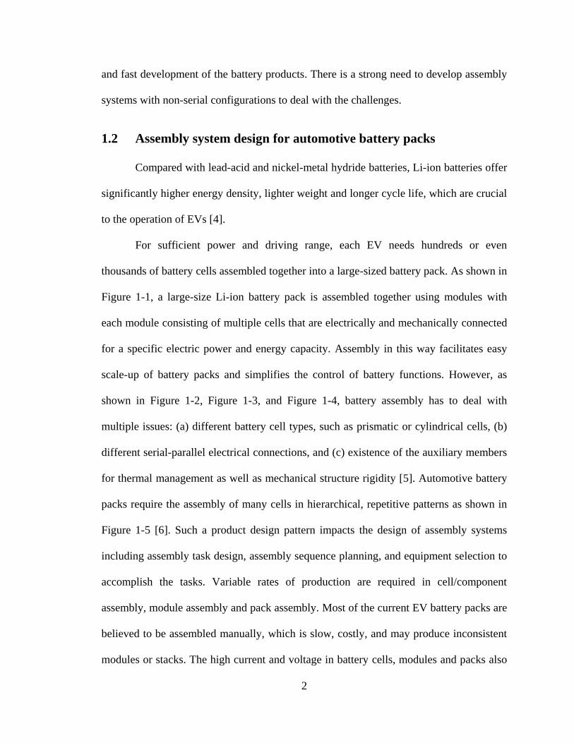
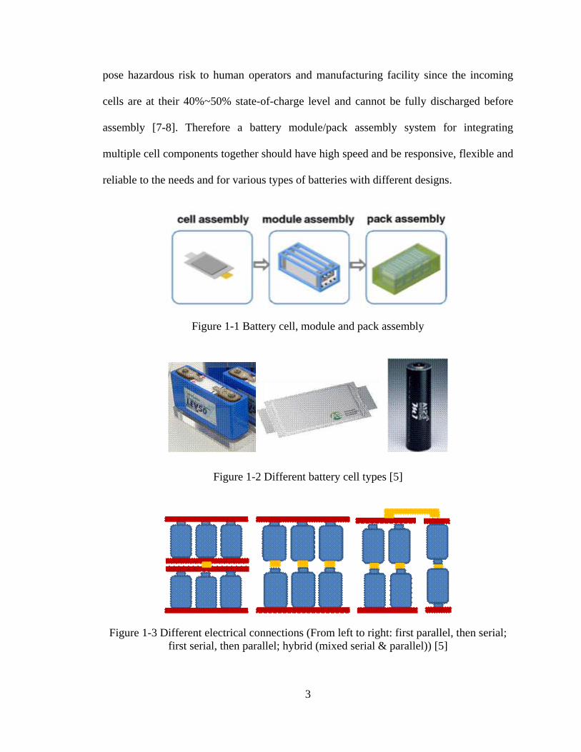

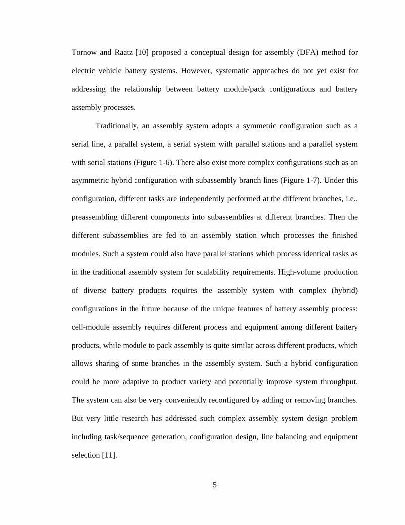


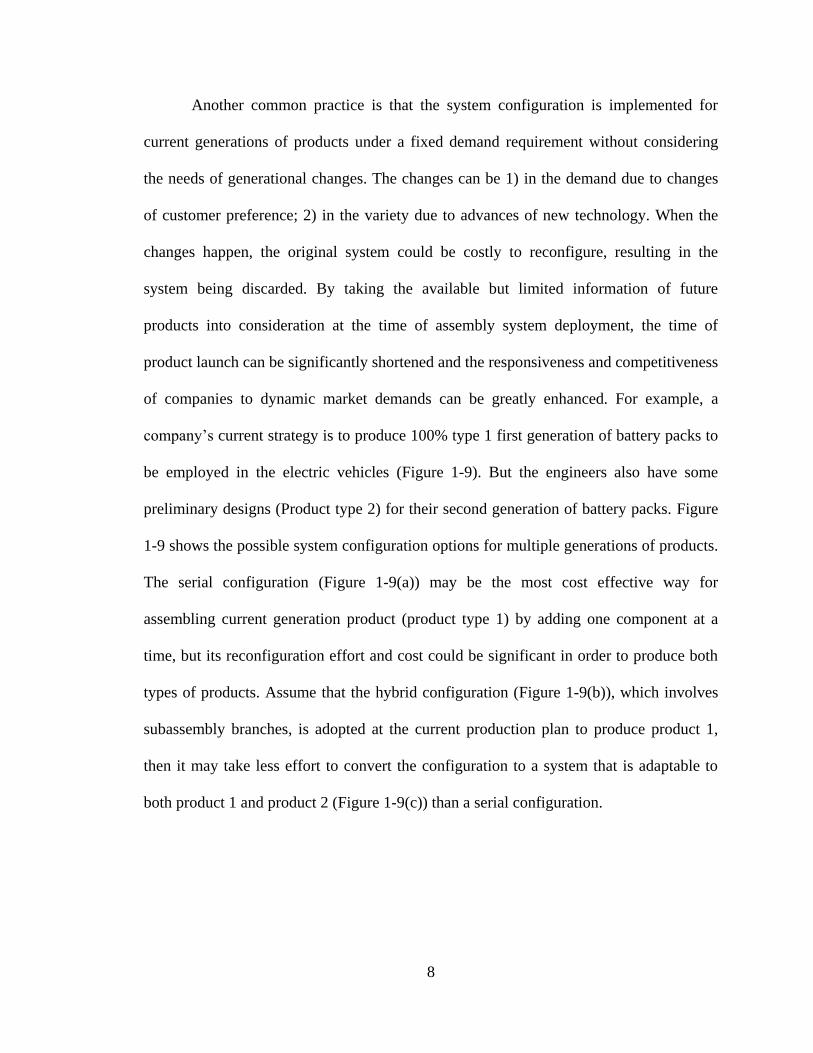
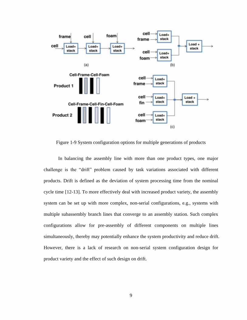
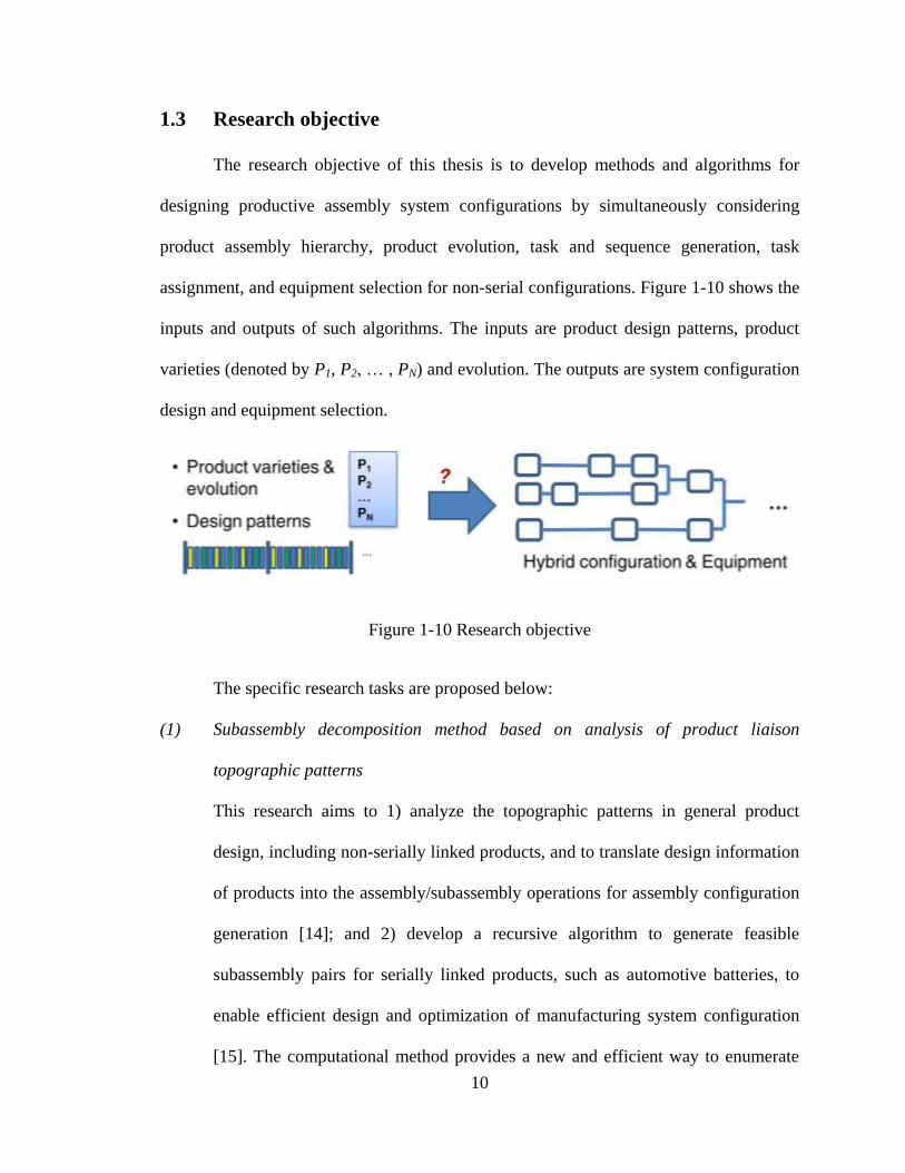


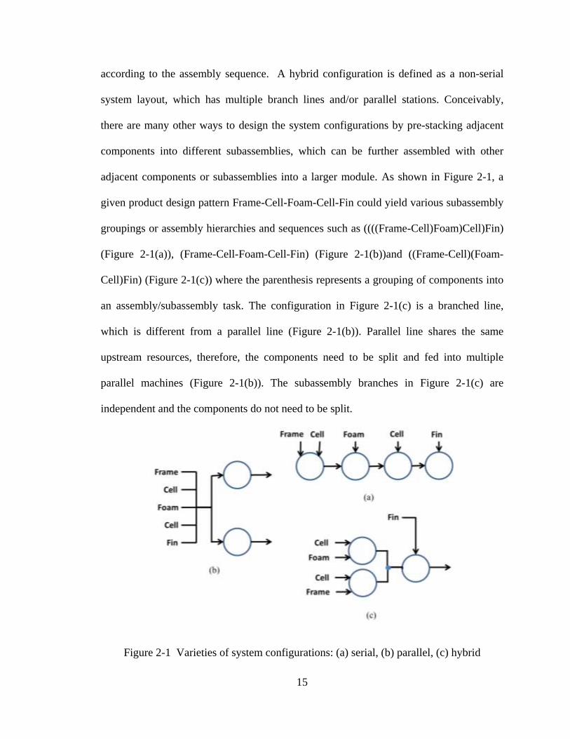
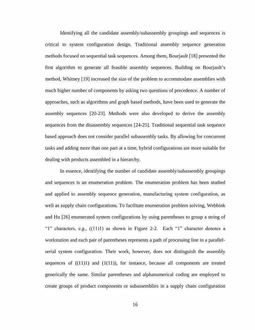
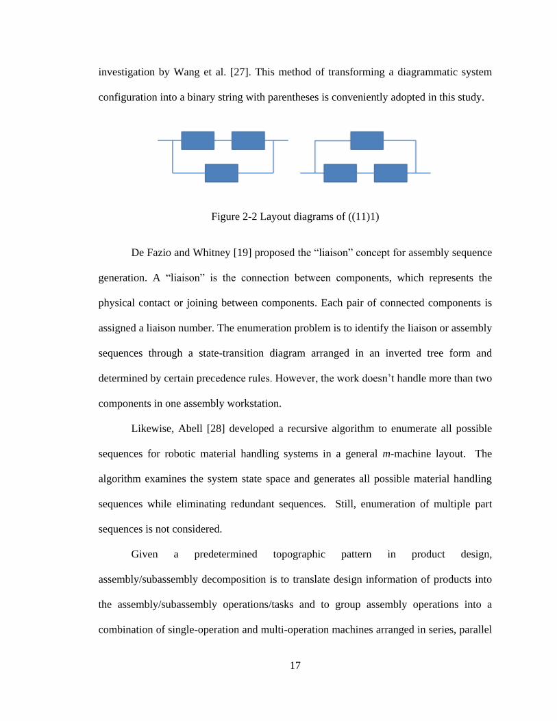

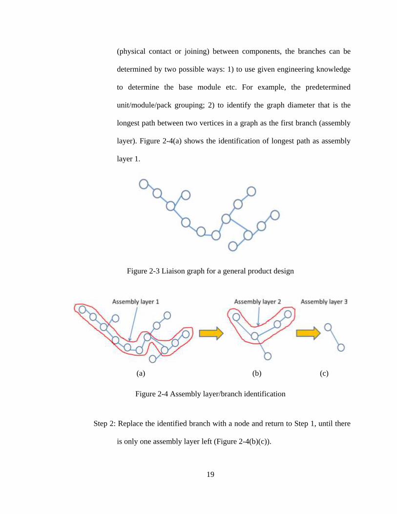


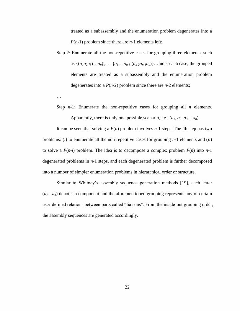

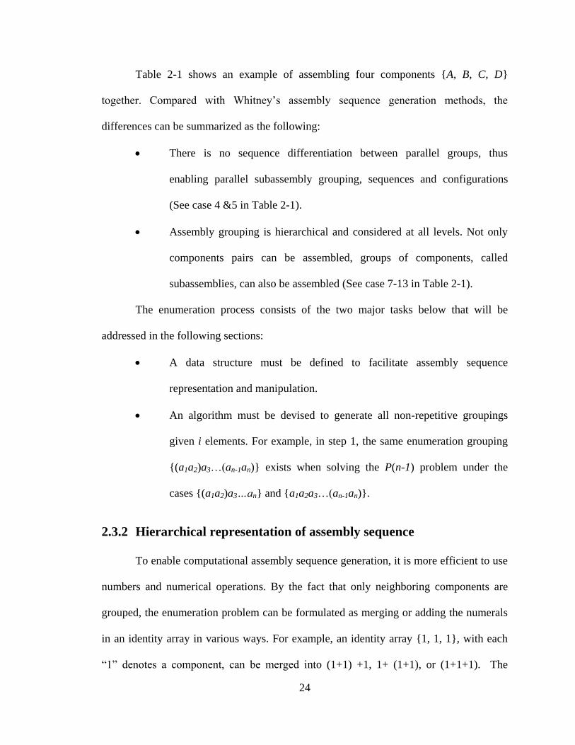

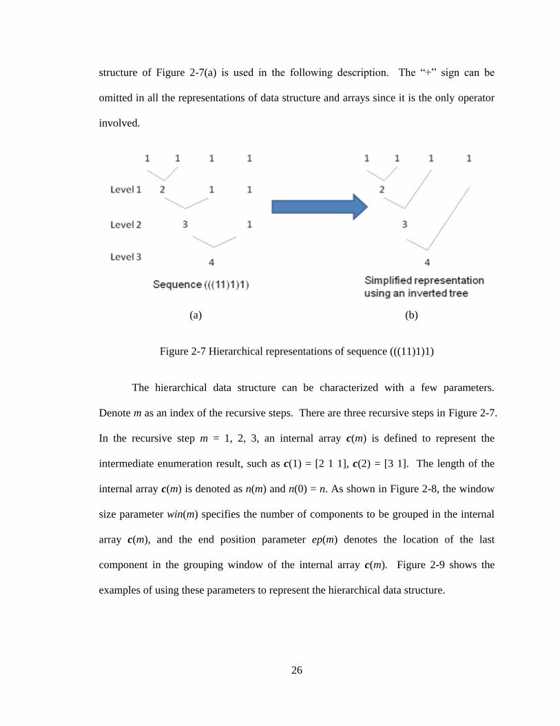


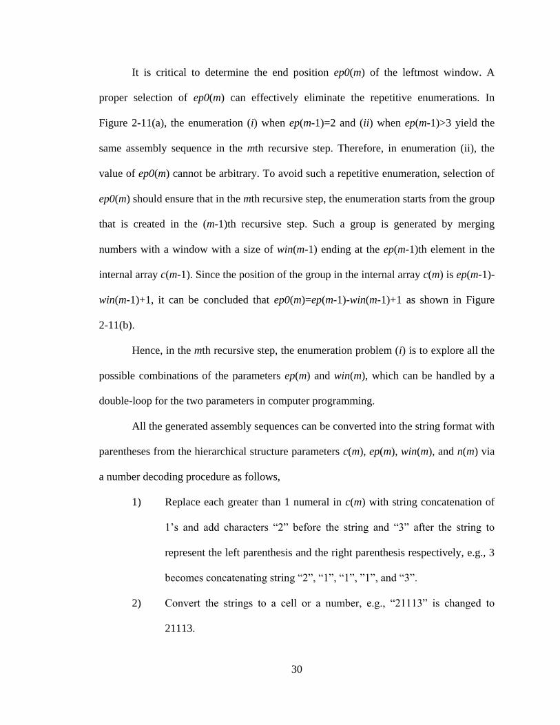


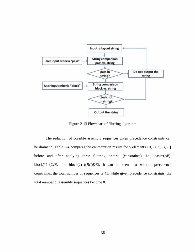


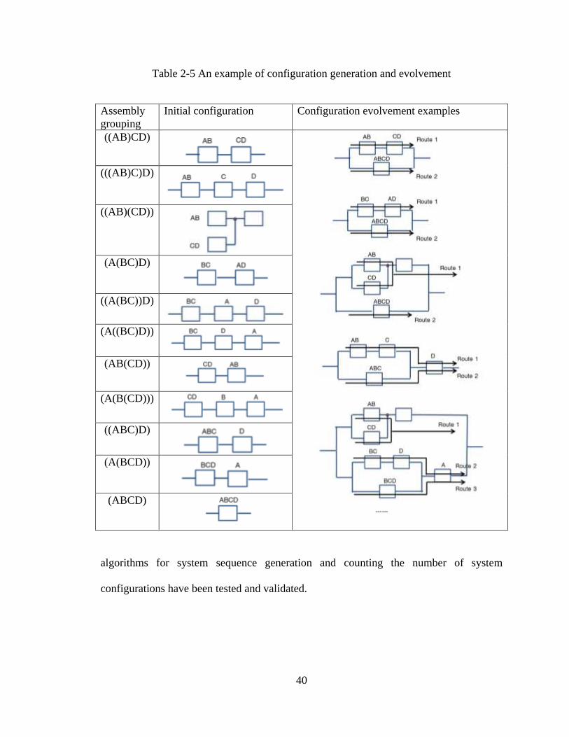

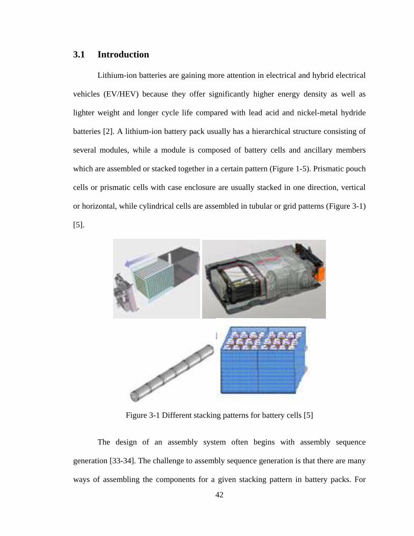
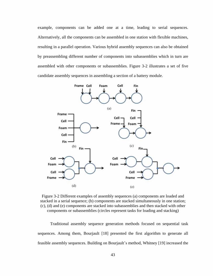

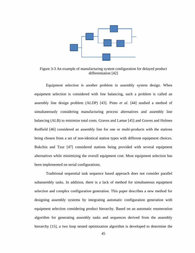
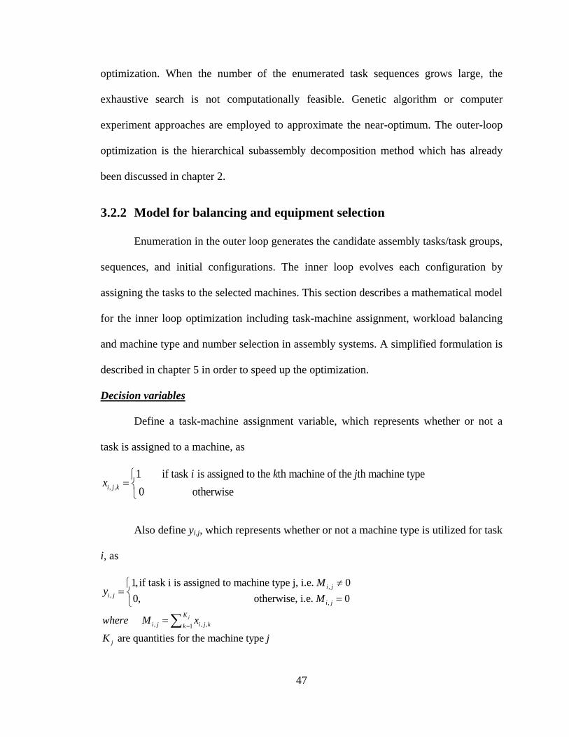


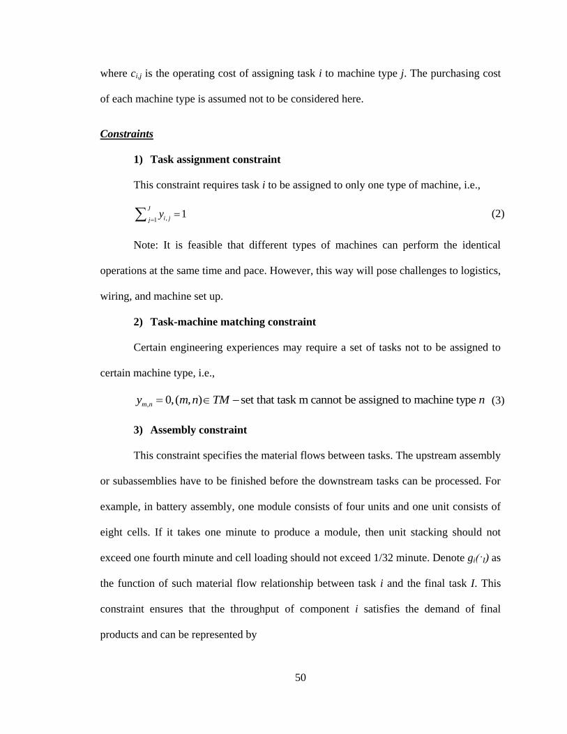

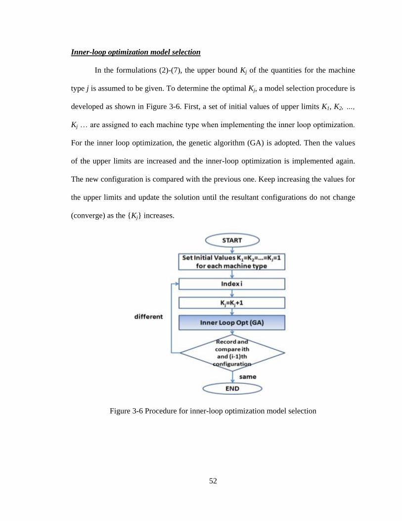


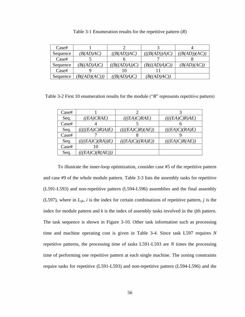


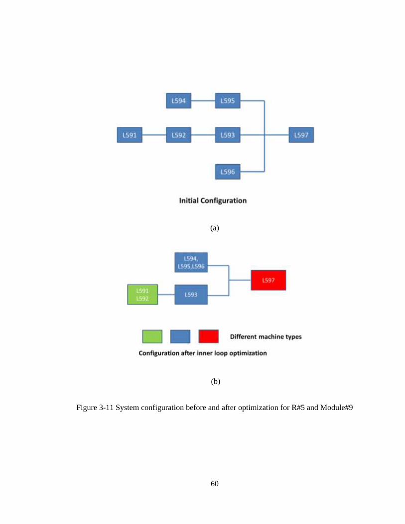

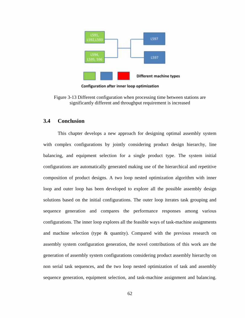


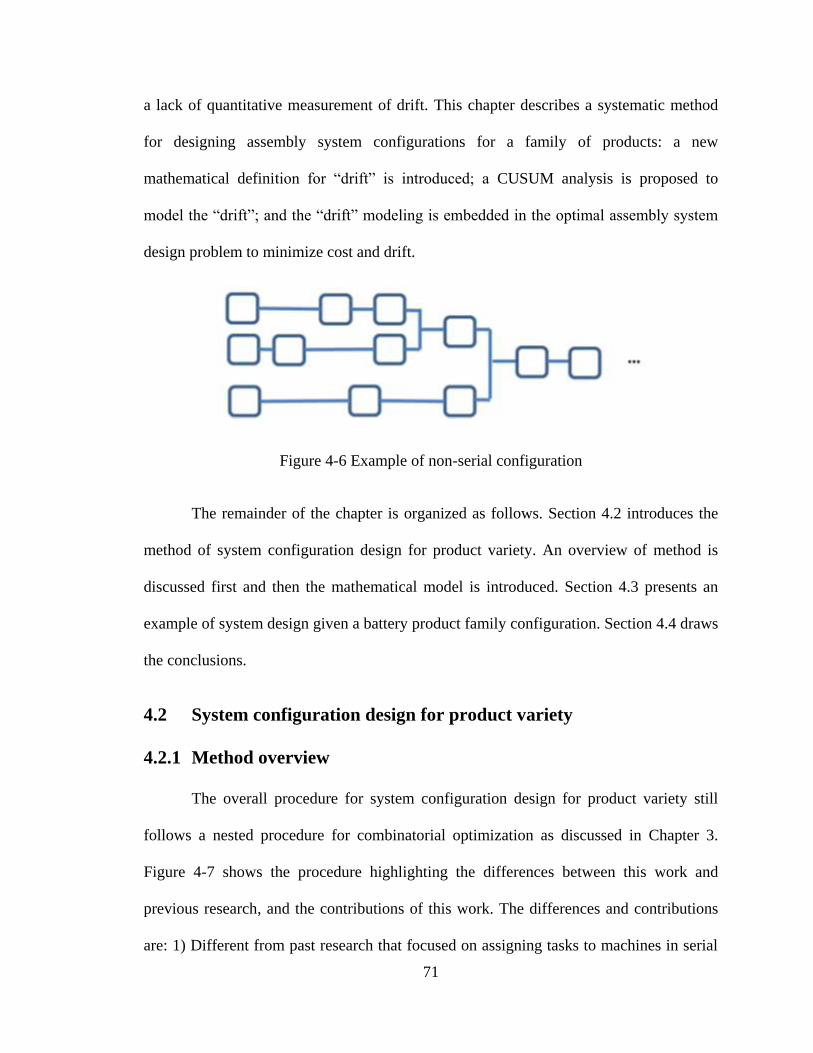
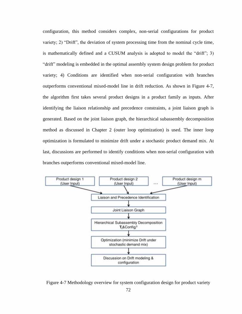
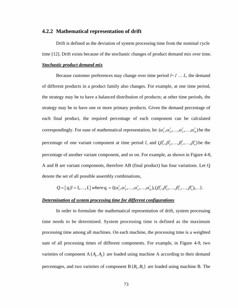

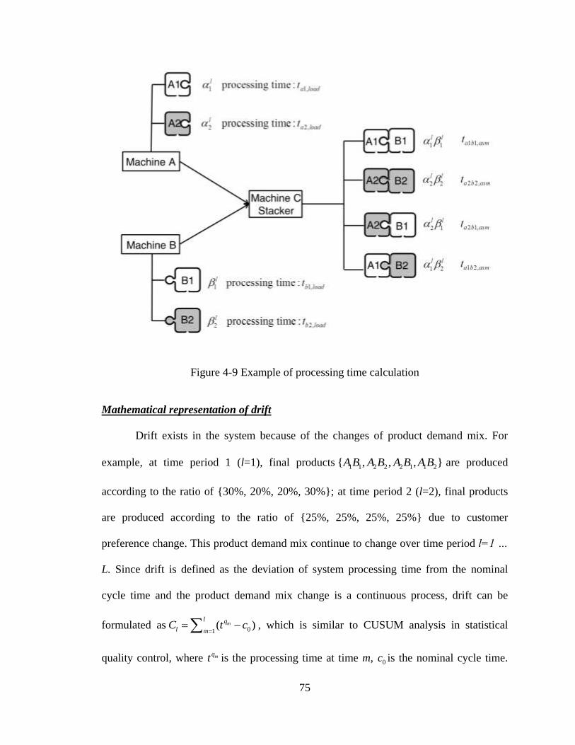

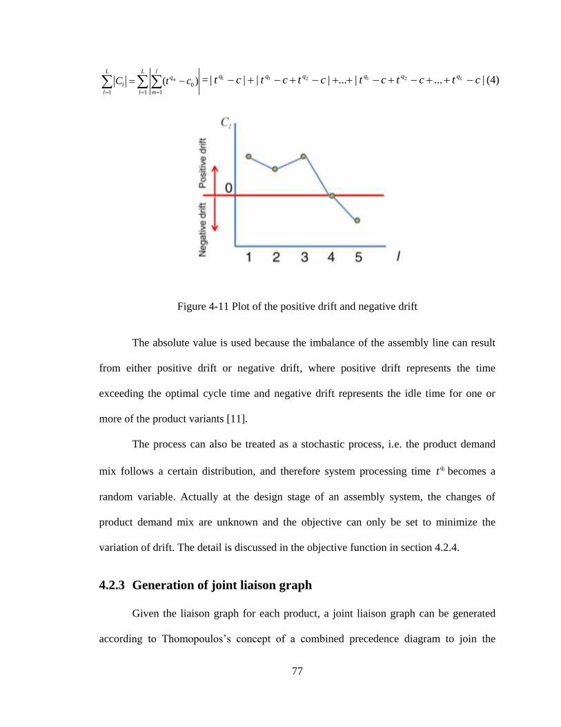


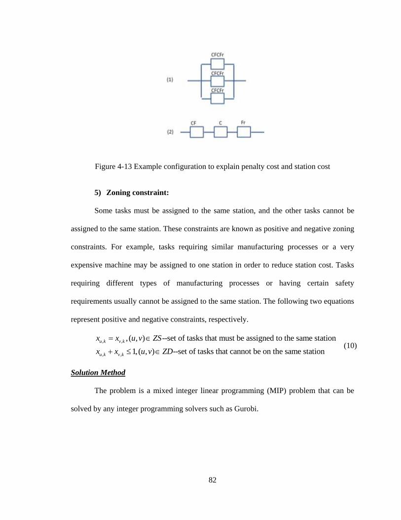

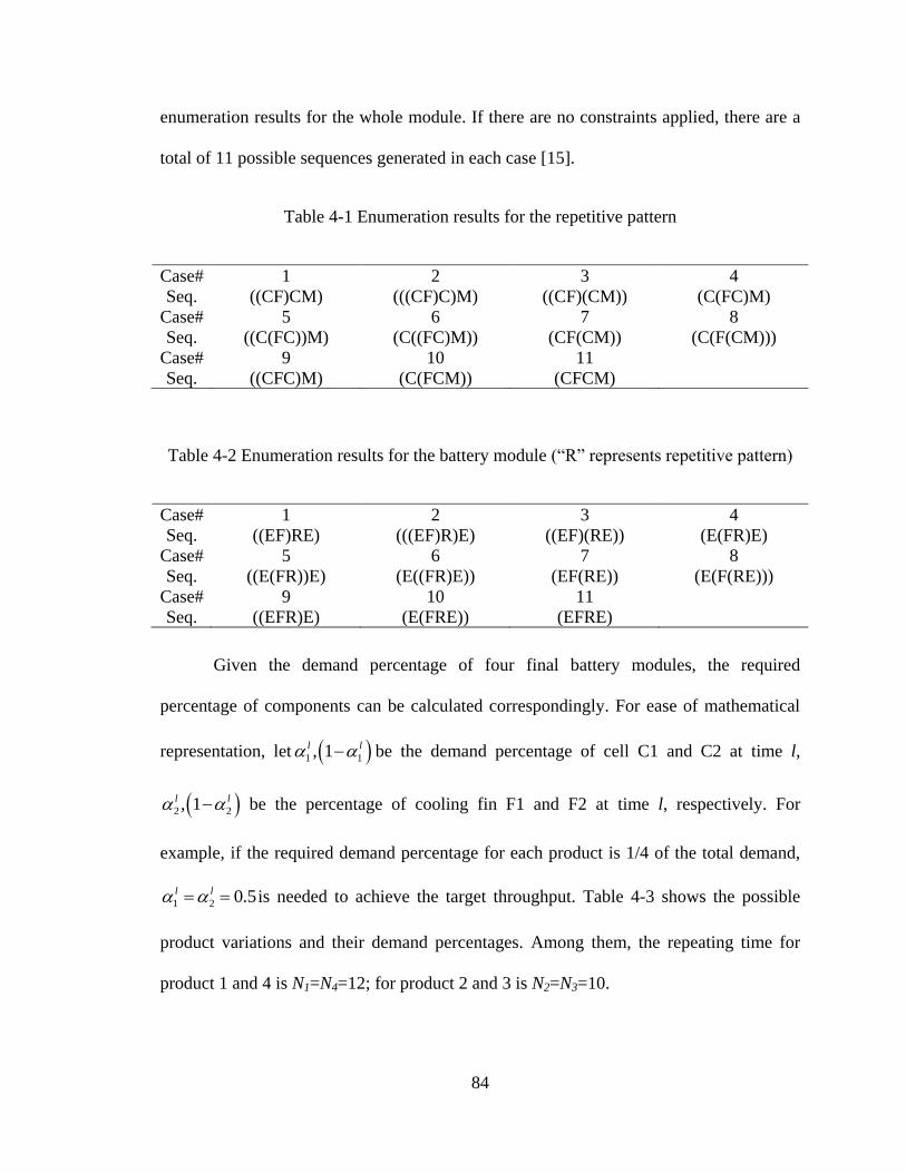


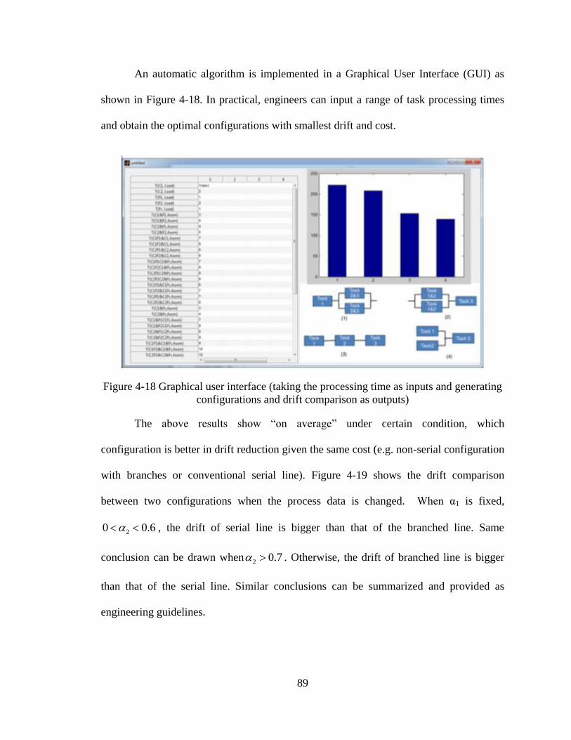


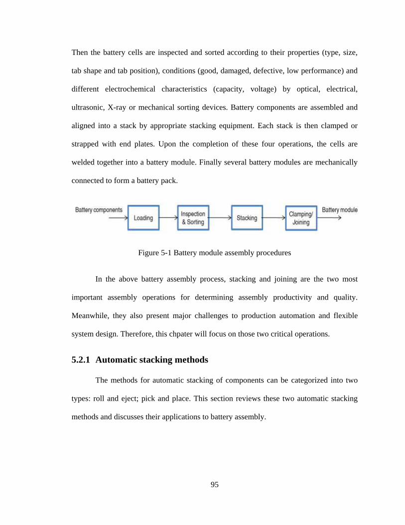


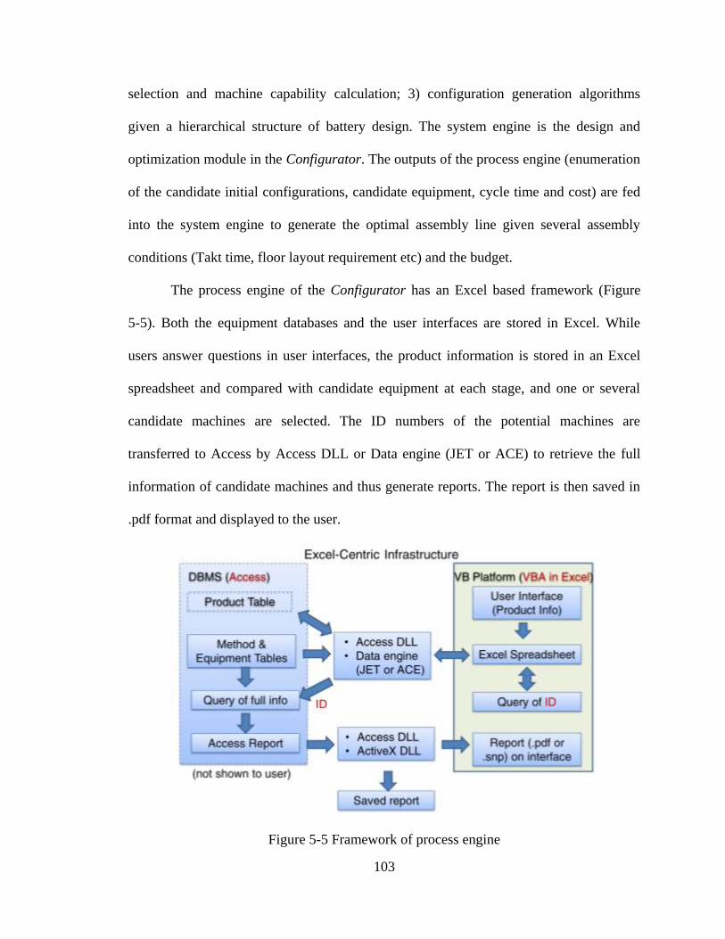
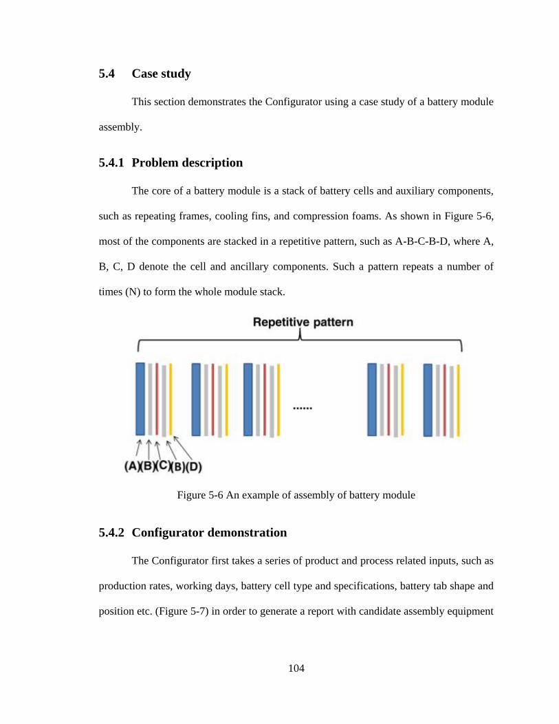


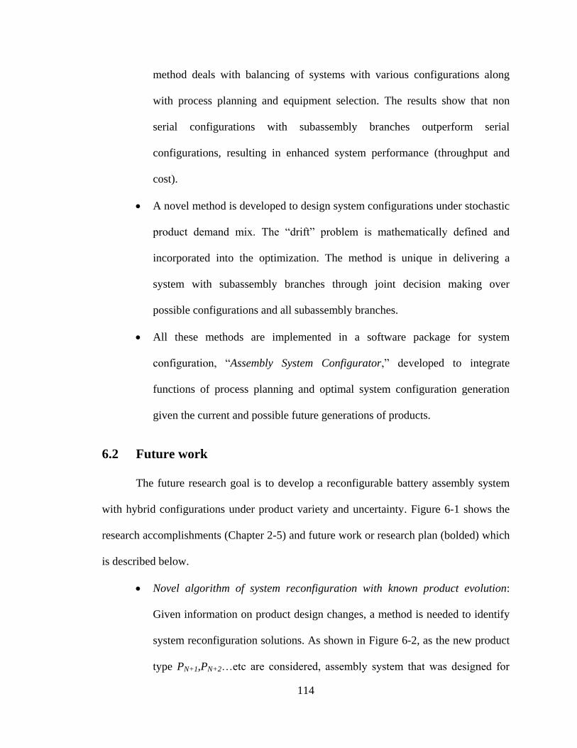
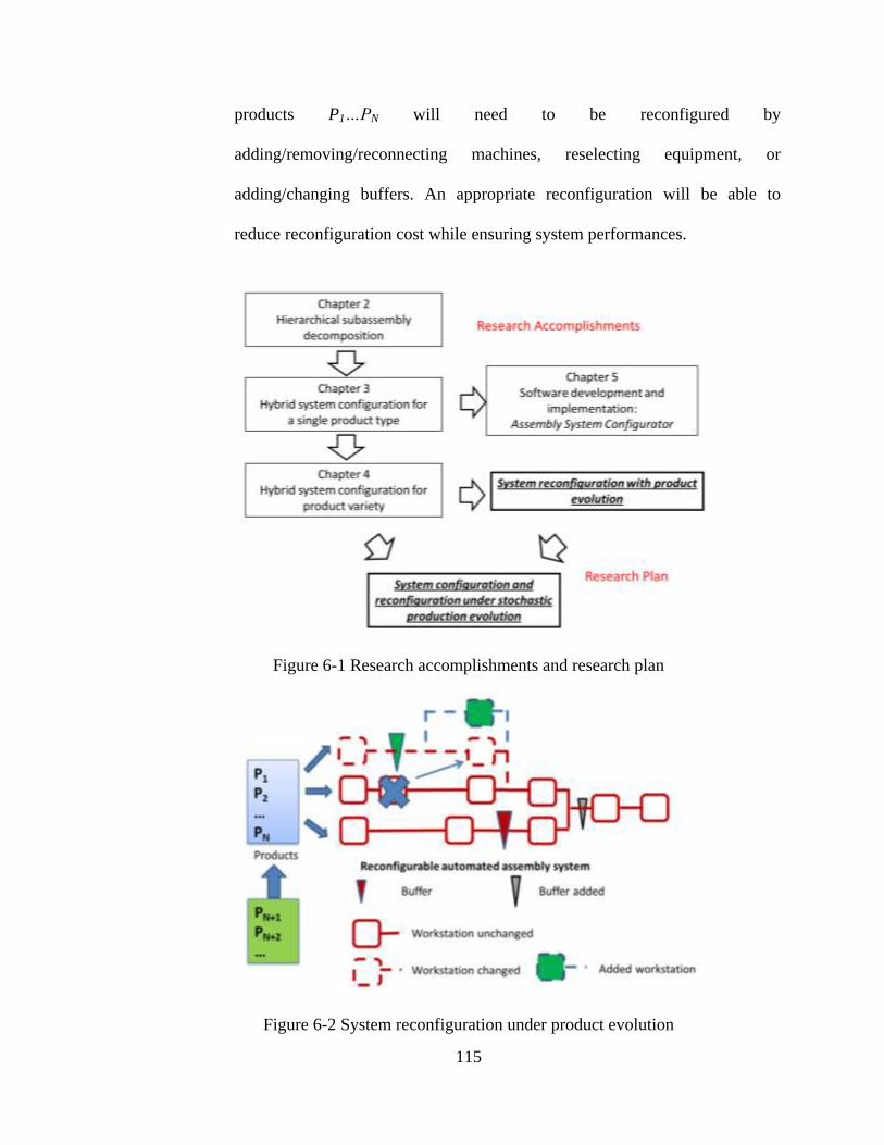


![Ondulé: Designing and Controlling 3D Printable Springs · HELICAL SPRING THEORY Our approach is based on helical springs [22], which have three basic configurations—compression,](https://static.documents.pub/doc/80x56/5e97e6d886fa3e4f6f1a5e42/ondul-designing-and-controlling-3d-printable-helical-spring-theory-our-approach.jpg)


