Desktop-4D-Toolbox (D4D) User Manual

Oguz Tanzer

October 8, 2002

http://syke.hut.fi/~tanzer/d4d

1

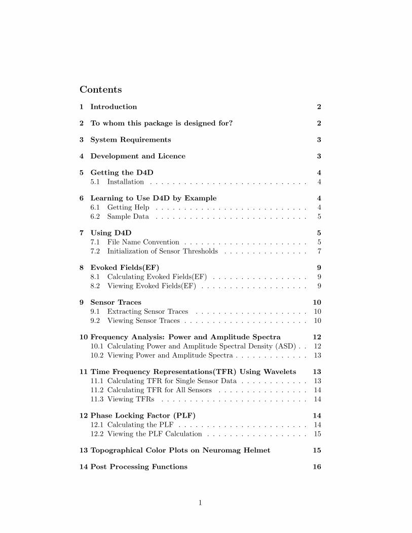
Contents

1 Introduction 2

2 To whom this package is designed for? 2

3 System Requirements 3

4 Development and Licence 3

5 Getting the D4D 45.1 Installation . . . . . . . . . . . . . . . . . . . . . . . . . . . . 4

6 Learning to Use D4D by Example 46.1 Getting Help . . . . . . . . . . . . . . . . . . . . . . . . . . . 46.2 Sample Data . . . . . . . . . . . . . . . . . . . . . . . . . . . 5

7 Using D4D 57.1 File Name Convention . . . . . . . . . . . . . . . . . . . . . . 57.2 Initialization of Sensor Thresholds . . . . . . . . . . . . . . . 7

8 Evoked Fields(EF) 98.1 Calculating Evoked Fields(EF) . . . . . . . . . . . . . . . . . 98.2 Viewing Evoked Fields(EF) . . . . . . . . . . . . . . . . . . . 9

9 Sensor Traces 109.1 Extracting Sensor Traces . . . . . . . . . . . . . . . . . . . . 109.2 Viewing Sensor Traces . . . . . . . . . . . . . . . . . . . . . . 10

10 Frequency Analysis: Power and Amplitude Spectra 1210.1 Calculating Power and Amplitude Spectral Density (ASD) . . 1210.2 Viewing Power and Amplitude Spectra . . . . . . . . . . . . . 13

11 Time Frequency Representations(TFR) Using Wavelets 1311.1 Calculating TFR for Single Sensor Data . . . . . . . . . . . . 1311.2 Calculating TFR for All Sensors . . . . . . . . . . . . . . . . 1411.3 Viewing TFRs . . . . . . . . . . . . . . . . . . . . . . . . . . 14

12 Phase Locking Factor (PLF) 1412.1 Calculating the PLF . . . . . . . . . . . . . . . . . . . . . . . 1412.2 Viewing the PLF Calculation . . . . . . . . . . . . . . . . . . 15

13 Topographical Color Plots on Neuromag Helmet 15

14 Post Processing Functions 16

1

1 Introduction

Desktop-4D-Toolbox (D4D) is a window based data analysis platform foranalyzing and visualizing magnetoencephalographic (MEG) data currentlysupporting Neuromag MEG Data. The analysis functions are based onscripts of 4D Toolbox by Ole Jensen and also employs the FIFF (NeuromagData Format) to MAT conversion routines which are developed by KimmoUutela and the public distribution is supported by Neuromag Ltd.

The goal of this tool is to create an efficient and organized data analyzingenvironment for research on MEG data for neuroscientists.

It is designed with the idea that, the collected data can be analyzedrelatively quickly by users with graphic handles such as edit boxes and datasliders.

The graphical user interface reduces the amount of repeated tasks byeliminating writing or changing of Matlab scripts to perform trivial opera-tions to analyze the MEG data at hand.

An important design concept was to enable or disable the user whenenough parameters are not present to analyze the given data. This includesthe disabling of the fields regarding the analyzing function when enoughparameters are not available.

Desktop-4D-Toolbox should also be well suited for unexperienced users,who want to learn about the effect of certain parameters on the MEG dataquickly.

2 To whom this package is designed for?

The D4D is designed especially for people without computer programmingor script programming background, but would like to analyze MEG datawith the tools provided with the 4D Toolbox.

Users with computer programming background, or who find this packagelimiting can also refer to the scripts of 4D-Toolbox. Users can also refer to4D-Toolbox manual for further information on availability of the tools.

The main features of the D4D include:

• Analyzing MEG data without writing scripts

• Better interaction with data using graphical adjustment of parametersand data hiding

• More organized data analysis

2

Machine Type Matlab version operating systemIBM-PC Matlab 6.1 LinuxIBM-PC Matlab 6.1 MS Windows 2000*

HP Matlab 6.1 HP-UX

Table 1: Machines and operating systems on which D4D has been tested (asof September 2002)

• Colored views of files in current directory with bookshelf approach

• Some data post-processing

• Changing graph view parameters for nice printouts (Future version)

• Usability under various environments with Matlab

3 System Requirements

The software is designed and written under Matlab and works under Matlab5.x and Matlab 6.x versions. It requires that the FIFF to Matlab routinesand 4-D Toolbox scripts are in the same directory as the D4D components.The raw FIFF to Matlab conversion routines are pre-compiled binaries aretested to work in HP-UX and Linux systems.Table 1 shows the platforms this package is tested. *Since D4D is imple-mented completely in Matlab, it is possible to use the package in any en-vironment where Matlab is supported, but the FIFF to Matlab conversionroutines currently work only under Linux and HP-UX. However, other data,saved in Matlab ”.MAT” format could be analyzed. For example, extracteddata could be sent to an MS Windows environment and other tasks couldbe performed.

4 Development and Licence

The D4D is designed and written by Oguz Tanzer at Laboratory of Biomed-ical Engineering, Helsinki University of Technology.The package is continuously updated so please check frequently for newfunction updates. It is user’s own responsibility to check the results of thepackage. This is a new distribution and bugs in the package are inevitable.Please report them to tanzer@syke.hut.fi also feedback is very valuableand encouraged.D4D is a free software (but not the conversion routines converting FIFF toMatlab format) This allows you to re-distribute and modify the functions

3

under the terms of the GNU general public licence as published by the FreeSoftware Foundation.

5 Getting the D4D

All the components of the software can be downloaded from the D4D web-page: http://syke.hut.fi/~tanzer/d4d

The D4D requires 4D-Toolbox(http://boojum.hut.fi/~ojensen/4Dtools)scripts and the FIFF to Matlab conversion routines(http://boojum.hut.fi/~kuutela/meg-pd/).Please refer to their individual web pages on specific information about thesesoftware.

5.1 Installation

Use the following command to unpack the .TAR file:

>tar -xf d4d.tar

and follow the appropriate instructions below. If you already have 4D-Toolbox installed skip step 1 etc.

Steps of a from scratch installation are as follows:

1. Install 4D-Toolbox http://boojum.hut.fi/~ojensen/4Dtools

2. Install FIFF access routines http://boojum.hut.fi/~kuutela/meg-pd/

3. Extract d4d.tar to the same directory where the 4D-Toolbox scriptsreside.

6 Learning to Use D4D by Example

In this section the components of the D4D is explained and how to use isexplained via an example tutorial. This tutorial is the D4D version of thesame material found in 4D-Toolbox manual. The same data file is used.The idea is that the user can perform the same operations as in 4D-Toolboxusing the user interface following the protocol of D4D.

6.1 Getting Help

A nice part of the D4D is that, user is provided with pop-up tips on whateach graphical object does. Also, each button is labelled intuitively regard-ing the function it performs.

4

6.2 Sample Data

The file mnStim150.fif used in the tutorial can be downloaded from theD4D webpage: http://syke.hut.fi/~tanzer/d4d or from the 4D-Toolboxwebpage: http://boojum.hut.fi/~ojensen/4DtoolsAfter downloading move the file to the working directory and unzip usingthe command:>gunzip mnStim150.fif.gzThe FIFF file mnStim150.fif contains raw MEG data recorded by Neuro-mag Vectorview system (306 sensors) and the data are from an experimentin which a subject received alternating stimuli to the left and right mediannerve at wrists. The times of left and right hand stimulation are respectivelymarked by trigger channel 1 and 2. There are about 200 stimuli per hand.The interstimulus interval was 3 second, each side. The data were digitizedat 600Hz [1].

7 Using D4D

Open Matlab and goto the directory where D4D and 4D-Toolbox are in-stalled. Enter command:

>d4d

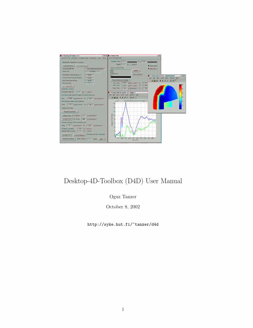
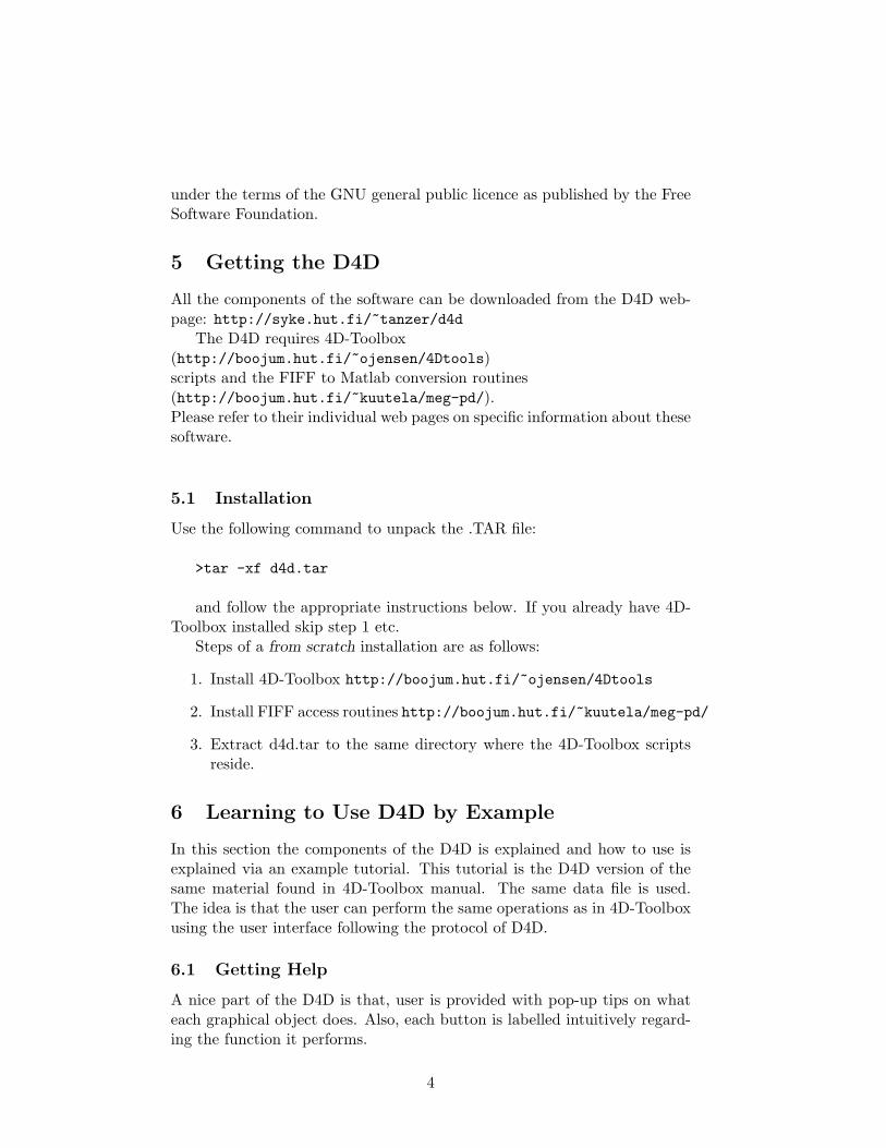
The main window shown in Figure 1 will come up and the program isready to start.

Make sure the data file is in the same directory as the programs files. Infuture versions possibly a separate data directory could be possible.

As explained above, the interface of D4D will be explained with an ex-ample. This is the same example found in 4D-Toolbox manual, so previoususers could be familiar to this one.

7.1 File Name Convention

The D4D has a unique but simple file naming convention with an aim toorganize the files after data analysis.

When an inputfile is loaded into the environment and an analysis isperformed on the loaded data, the type of analysis is embedded into theoutput filename. A distinct view of the output data files in the current di-rectory can be seen by pressing Show Available Data menu option on themain window. This results in the available data file window shown in Fig-ure 2

5

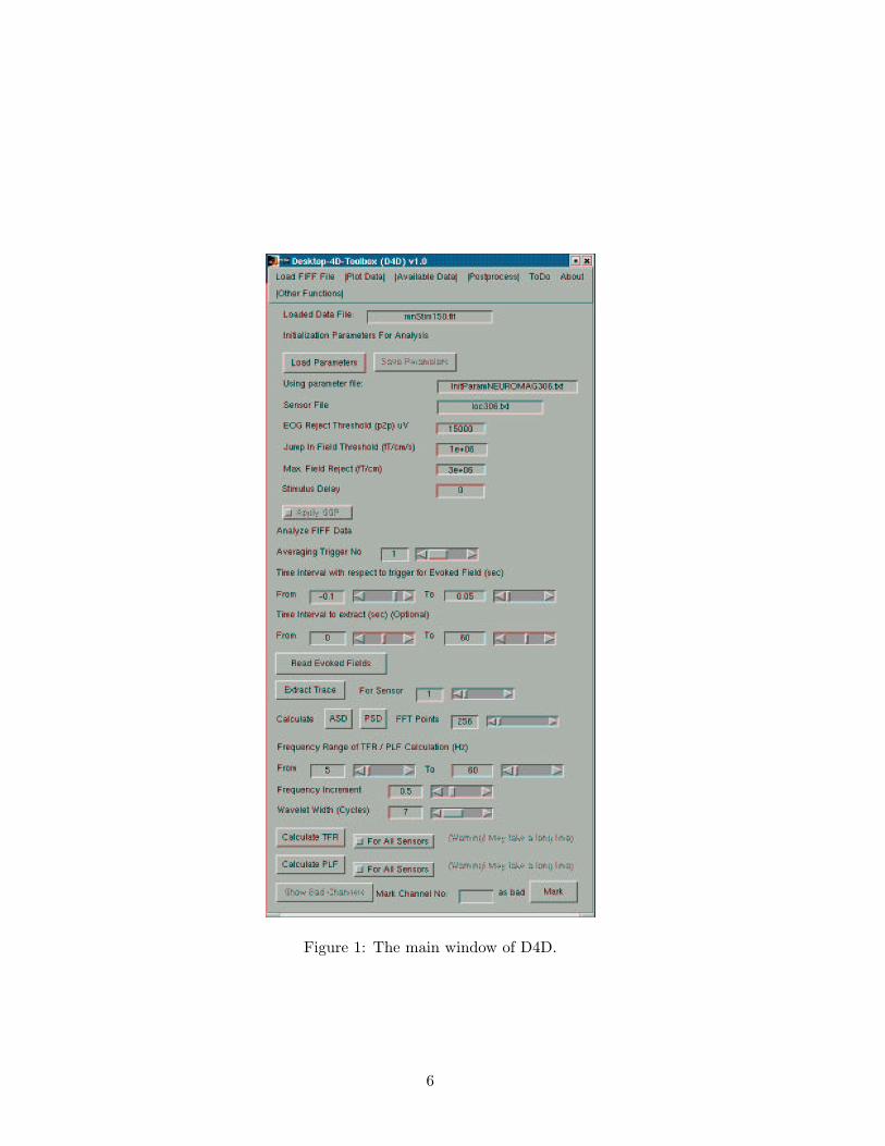
Figure 1: The main window of D4D.

6

In this example case, the input filename is mnStim150.fif. Accordinglythe output filename would be;

For Evoked Field of 1st Trigger:out_ef_trig1_mnStim150.fifFor Single Sensor Trace of 1st Trigger for Sensor 1:out_trace_trig1_sensor1_mnStim150.fif

These files can be seen from the Available Data menu option (Figure 1)once created.

In general the naming convention of the output files go as;

For Evoked Fields: out_ef_trig<#>_<inputfile>

For Single Sensor Traces: out_trace_trig<#>_sensor<#>_<inputfile>

For Amplitude Spectral Density: out_asd_<inputfile>

For Power Spectral Density: out_psd_<inputfile>

For Time Freq. Representation of 1 Sensor:

out_tfr_trig<#>_sensor<#>_<inputfile>

For Time Freq. Representation of All Sensors:

out_tfr_trig<#>_all_<inputfile>

7.2 Initialization of Sensor Thresholds

The parameters which define the threshold setting for the sensor rejectionare displayed on the upper part of the main window as shown in Figure 3.The version 1.0 of the D4D does not allow changing of these parametersfrom the GUI.If you want change some rejection parameters, simply open the parameterfile shown in Figure 3 and edit the fields with a text editor. It is hoped thatthe future version will enable changing these from the user interface.

7

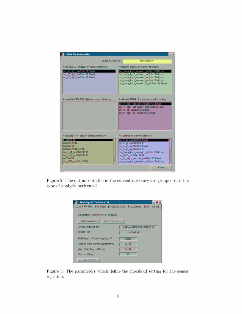
Figure 2: The output data file in the current directory are grouped into thetype of analysis performed.

Figure 3: The parameters which define the threshold setting for the sensorrejection.

8

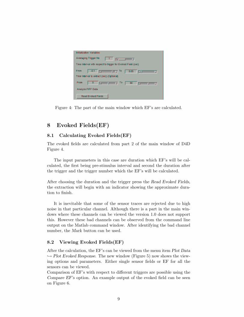
Figure 4: The part of the main window which EF’s are calculated.

8 Evoked Fields(EF)

8.1 Calculating Evoked Fields(EF)

The evoked fields are calculated from part 2 of the main window of D4DFigure 4.

The input parameters in this case are duration which EF’s will be cal-culated, the first being pre-stimulus interval and second the duration afterthe trigger and the trigger number which the EF’s will be calculated.

After choosing the duration and the trigger press the Read Evoked Fields,the extraction will begin with an indicator showing the approximate dura-tion to finish.

It is inevitable that some of the sensor traces are rejected due to highnoise in that particular channel. Although there is a part in the main win-dows where these channels can be viewed the version 1.0 does not supportthis. However these bad channels can be observed from the command lineoutput on the Matlab command window. After identifying the bad channelnumber, the Mark button can be used.

8.2 Viewing Evoked Fields(EF)

After the calculation, the EF’s can be viewed from the menu item Plot Data↪→ Plot Evoked Response. The new window (Figure 5) now shows the view-ing options and parameters. Either single sensor fields or EF for all thesensors can be viewed.Comparison of EF’s with respect to different triggers are possible using theCompare EF’s option. An example output of the evoked field can be seenon Figure 6.

9

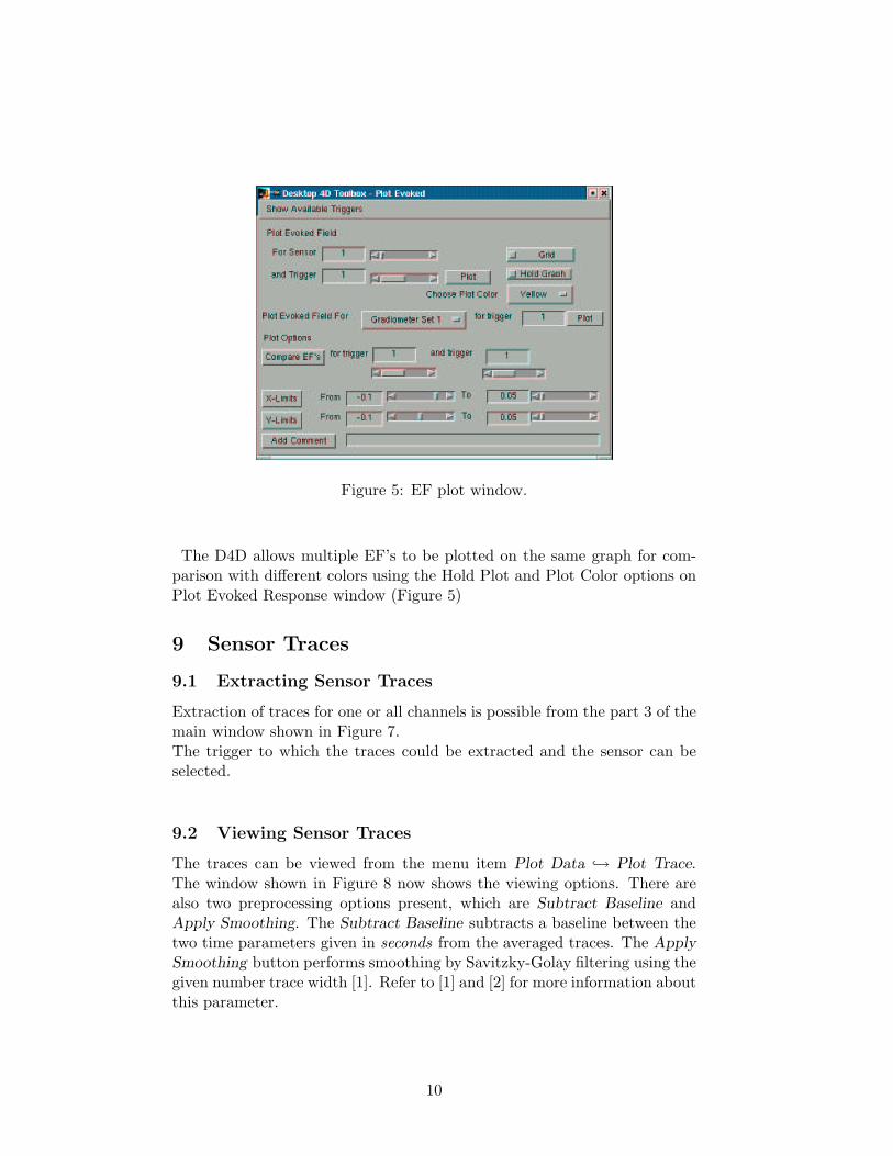
Figure 5: EF plot window.

The D4D allows multiple EF’s to be plotted on the same graph for com-parison with different colors using the Hold Plot and Plot Color options onPlot Evoked Response window (Figure 5)

9 Sensor Traces

9.1 Extracting Sensor Traces

Extraction of traces for one or all channels is possible from the part 3 of themain window shown in Figure 7.The trigger to which the traces could be extracted and the sensor can beselected.

9.2 Viewing Sensor Traces

The traces can be viewed from the menu item Plot Data ↪→ Plot Trace.The window shown in Figure 8 now shows the viewing options. There arealso two preprocessing options present, which are Subtract Baseline andApply Smoothing. The Subtract Baseline subtracts a baseline between thetwo time parameters given in seconds from the averaged traces. The ApplySmoothing button performs smoothing by Savitzky-Golay filtering using thegiven number trace width [1]. Refer to [1] and [2] for more information aboutthis parameter.

10

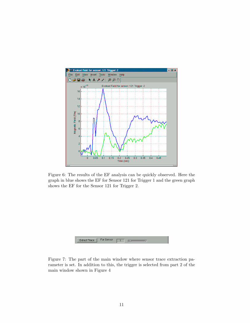
Figure 6: The results of the EF analysis can be quickly observed. Here thegraph in blue shows the EF for Sensor 121 for Trigger 1 and the green graphshows the EF for the Sensor 121 for Trigger 2.

Figure 7: The part of the main window where sensor trace extraction pa-rameter is set. In addition to this, the trigger is selected from part 2 of themain window shown in Figure 4

11

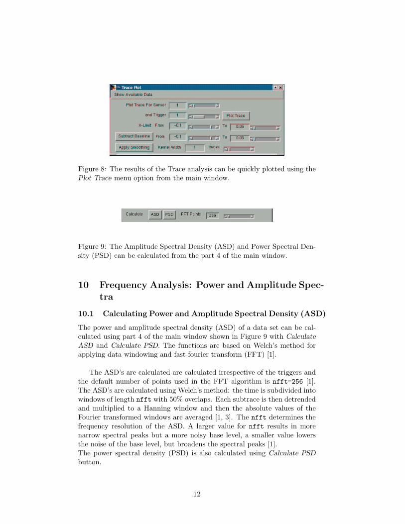
Figure 8: The results of the Trace analysis can be quickly plotted using thePlot Trace menu option from the main window.

Figure 9: The Amplitude Spectral Density (ASD) and Power Spectral Den-sity (PSD) can be calculated from the part 4 of the main window.

10 Frequency Analysis: Power and Amplitude Spec-tra

10.1 Calculating Power and Amplitude Spectral Density (ASD)

The power and amplitude spectral density (ASD) of a data set can be cal-culated using part 4 of the main window shown in Figure 9 with CalculateASD and Calculate PSD. The functions are based on Welch’s method forapplying data windowing and fast-fourier transform (FFT) [1].

The ASD’s are calculated are calculated irrespective of the triggers andthe default number of points used in the FFT algorithm is nfft=256 [1].The ASD’s are calculated using Welch’s method: the time is subdivided intowindows of length nfft with 50% overlaps. Each subtrace is then detrendedand multiplied to a Hanning window and then the absolute values of theFourier transformed windows are averaged [1, 3]. The nfft determines thefrequency resolution of the ASD. A larger value for nfft results in morenarrow spectral peaks but a more noisy base level, a smaller value lowersthe noise of the base level, but broadens the spectral peaks [1].The power spectral density (PSD) is also calculated using Calculate PSDbutton.

12

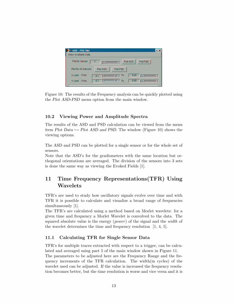
Figure 10: The results of the Frequency analysis can be quickly plotted usingthe Plot ASD-PSD menu option from the main window.

10.2 Viewing Power and Amplitude Spectra

The results of the ASD and PSD calculation can be viewed from the menuitem Plot Data ↪→ Plot ASD and PSD. The window (Figure 10) shows theviewing options.

The ASD and PSD can be plotted for a single sensor or for the whole set ofsensors.Note that the ASD’s for the gradiometers with the same location but or-thogonal orientations are averaged. The division of the sensors into 3 setsis done the same way as viewing the Evoked Fields [1].

11 Time Frequency Representations(TFR) UsingWavelets

TFR’s are used to study how oscillatory signals evolve over time and withTFR it is possible to calculate and visualize a broad range of frequenciessimultaneously [1].The TFR’s are calculated using a method based on Morlet wavelets: for agiven time and frequency a Morlet Wavelet is convolved to the data. Thesquared absolute value is the energy (power) of the signal and the width ofthe wavelet determines the time and frequency resolution [1, 4, 5].

11.1 Calculating TFR for Single Sensor Data

TFR’s for multiple traces extracted with respect to a trigger, can be calcu-lated and averaged using part 5 of the main window shown in Figure 11.The parameters to be adjusted here are the Frequency Range and the fre-quency increments of the TFR calculation. The width(in cycles) of thewavelet used can be adjusted. If the value is increased the frequency resolu-tion becomes better, but the time resolution is worse and vice versa and it is

13

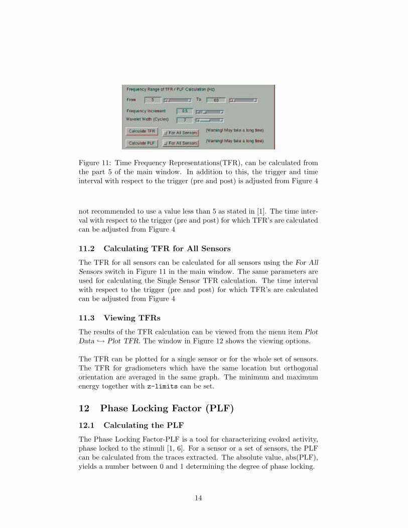
Figure 11: Time Frequency Representations(TFR), can be calculated fromthe part 5 of the main window. In addition to this, the trigger and timeinterval with respect to the trigger (pre and post) is adjusted from Figure 4

not recommended to use a value less than 5 as stated in [1]. The time inter-val with respect to the trigger (pre and post) for which TFR’s are calculatedcan be adjusted from Figure 4

11.2 Calculating TFR for All Sensors

The TFR for all sensors can be calculated for all sensors using the For AllSensors switch in Figure 11 in the main window. The same parameters areused for calculating the Single Sensor TFR calculation. The time intervalwith respect to the trigger (pre and post) for which TFR’s are calculatedcan be adjusted from Figure 4

11.3 Viewing TFRs

The results of the TFR calculation can be viewed from the menu item PlotData ↪→ Plot TFR. The window in Figure 12 shows the viewing options.

The TFR can be plotted for a single sensor or for the whole set of sensors.The TFR for gradiometers which have the same location but orthogonalorientation are averaged in the same graph. The minimum and maximumenergy together with z-limits can be set.

12 Phase Locking Factor (PLF)

12.1 Calculating the PLF

The Phase Locking Factor-PLF is a tool for characterizing evoked activity,phase locked to the stimuli [1, 6]. For a sensor or a set of sensors, the PLFcan be calculated from the traces extracted. The absolute value, abs(PLF),yields a number between 0 and 1 determining the degree of phase locking.

14

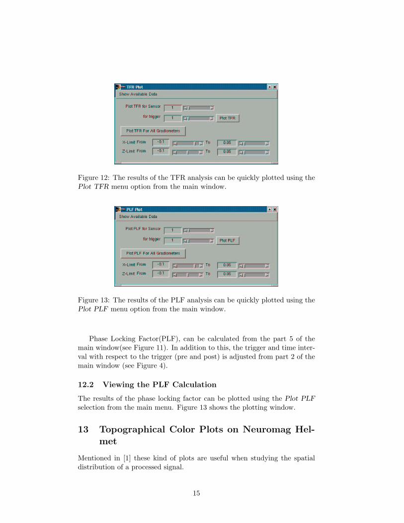
Figure 12: The results of the TFR analysis can be quickly plotted using thePlot TFR menu option from the main window.

Figure 13: The results of the PLF analysis can be quickly plotted using thePlot PLF menu option from the main window.

Phase Locking Factor(PLF), can be calculated from the part 5 of themain window(see Figure 11). In addition to this, the trigger and time inter-val with respect to the trigger (pre and post) is adjusted from part 2 of themain window (see Figure 4).

12.2 Viewing the PLF Calculation

The results of the phase locking factor can be plotted using the Plot PLFselection from the main menu. Figure 13 shows the plotting window.

13 Topographical Color Plots on Neuromag Hel-met

Mentioned in [1] these kind of plots are useful when studying the spatialdistribution of a processed signal.

15

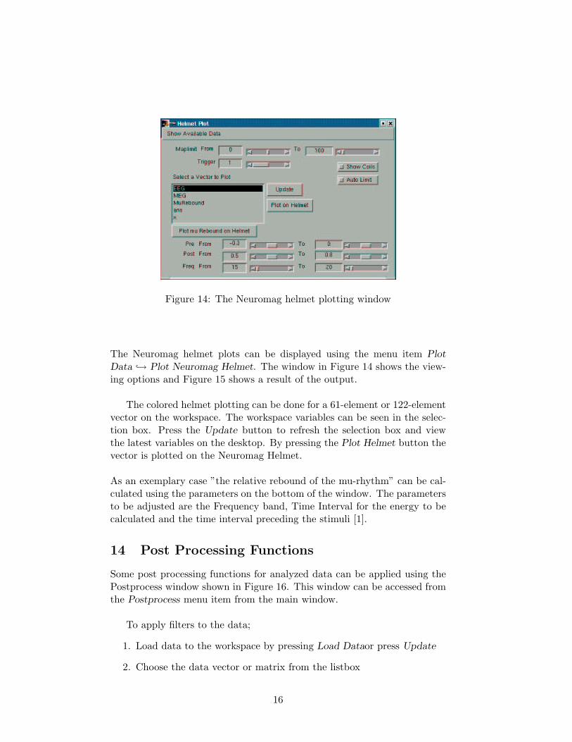
Figure 14: The Neuromag helmet plotting window

The Neuromag helmet plots can be displayed using the menu item PlotData ↪→ Plot Neuromag Helmet. The window in Figure 14 shows the view-ing options and Figure 15 shows a result of the output.

The colored helmet plotting can be done for a 61-element or 122-elementvector on the workspace. The workspace variables can be seen in the selec-tion box. Press the Update button to refresh the selection box and viewthe latest variables on the desktop. By pressing the Plot Helmet button thevector is plotted on the Neuromag Helmet.

As an exemplary case ”the relative rebound of the mu-rhythm” can be cal-culated using the parameters on the bottom of the window. The parametersto be adjusted are the Frequency band, Time Interval for the energy to becalculated and the time interval preceding the stimuli [1].

14 Post Processing Functions

Some post processing functions for analyzed data can be applied using thePostprocess window shown in Figure 16. This window can be accessed fromthe Postprocess menu item from the main window.

To apply filters to the data;

1. Load data to the workspace by pressing Load Dataor press Update

2. Choose the data vector or matrix from the listbox

16

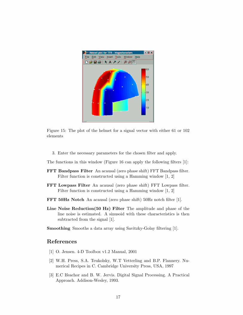
Figure 15: The plot of the helmet for a signal vector with either 61 or 102elements

3. Enter the necessary parameters for the chosen filter and apply.

The functions in this window (Figure 16 can apply the following filters [1]:

FFT Bandpass Filter An acausal (zero phase shift) FFT Bandpass filter.Filter function is constructed using a Hamming window [1, 2]

FFT Lowpass Filter An acausal (zero phase shift) FFT Lowpass filter.Filter function is constructed using a Hamming window [1, 2]

FFT 50Hz Notch An acausal (zero phase shift) 50Hz notch filter [1].

Line Noise Reduction(50 Hz) Filter The amplitude and phase of theline noise is estimated. A sinusoid with these characteristics is thensubtracted from the signal [1].

Smoothing Smooths a data array using Savitzky-Golay filtering [1].

References

[1] O. Jensen. 4-D Toolbox v1.2 Manual, 2001

[2] W.H. Press, S.A. Teukolsky, W.T Vetterling and B.P. Flannery. Nu-merical Recipes in C. Cambridge University Press, USA, 1997

[3] E.C Ifeachor and B. W. Jervis. Digital Signal Processing. A PracticalApproach. Addison-Wesley, 1993.

17

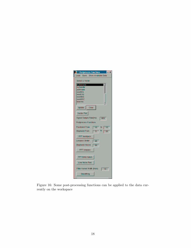
Figure 16: Some post-processing functions can be applied to the data cur-rently on the workspace

18

[4] J. Sinkkonen, H. Tiitinen and R. Naatanen. Gabor Filters: an informa-tive way for analysing event-related brain activity. J Neurosci Methods,56(1):99-104, Jan 1995

[5] C. Tallon Baudry, O. Bertrand, C. Delpuech and J. Pernier. Oscilla-tory gamma band(30-70 Hz) activity induced by a visual search task inhumans. J Neurosci, 17(2):722-734, Jan 1997

[6] C. Tallon Baudry, O. Bertrand, C. Delpuech and J. Pernier. StimulusSpecificity of phase-locked and non-phase locked 40 Hz visual responsesin human. J Neurosci, 16(13):4240-4249, Jan 1996

19