Detailed Analysis for Indirect Land Use Change Carbon intensities are calculated under the LCFS on a full life cycle basis. This means that the carbon intensity value assigned to each fuel reflects the GHG emissions associated with that fuel’s production, transport, storage, and use. Traditionally, only these steps, termed direct effects, have been included in the life cycle assessment of transportation fuels. In addition to these direct effects, some fuel production processes generate GHGs indirectly, via intermediate market mechanisms. Stakeholders participating in the LCFS process have suggested that most or all transportation fuels generate varying levels of indirect GHG emissions. To date, however, ARB staff has only identified one indirect effect that has a measurable impact on GHG emissions: land use change effects. A land use change effect is initially triggered when an increase in the demand for a crop-based biofuel begins to drive up prices for the necessary feedstock crop. This price increase causes farmers to devote a larger proportion of their cultivated acreage to that feedstock crop. Supplies of the displaced food and feed commodities subsequently decline, leading to higher prices for those commodities. Some of the options for many farmers to take advantage of these higher commodity prices are to take measures to increase yields, switch to growing crops with higher returns, and to bring non-agricultural lands into production. When new land is converted, such conversions release the carbon sequestered in soils and vegetation. The resulting carbon emissions constitute the “indirect” land use change (iLUC) impact of increased biofuel production. Based on research and published work, most of the land use change impacts result from the diversion of food crops to producing biofuels. During the regulatory process (i.e., workshops and meetings with stakeholders) leading up to the 2009 LCFS Board Hearing, the magnitude of this impact was discussed and also questioned by renewable fuel advocates. Land use change is driven by multiple factors, some of them not related to the production of biofuels. Because the tools for estimating land use change were few and relatively new when the regulation was originally adopted in 2009, biofuel producers argued that land use change impacts should be excluded from carbon intensity values, pending the development of better estimation techniques. Based on its work with land use change academics and researchers, however, ARB staff concluded that the land use impacts of crop-based biofuels were significant, and must be included in LCFS fuel carbon intensities. To exclude them would assume that there is zero impact resulting from the production of biofuels and would allow fuels with carbon intensities that are similar to gasoline and diesel fuel to function as low-carbon fuels under the LCFS. This would delay the development of truly low-carbon fuels, and by not accounting for the GHG emissions from land use change, would jeopardize the achievement of a ten percent reduction in fuel carbon intensity by 2020. Details of ARB’s estimated land use change impacts of biofuel crop production for the 2009 regulation is provided in the ISOR from 2009 1 . Since 2009, there have been numerous peer-reviewed publications, dissertations, and other scientific literature, that have focused on various aspects of indirect land use 1 See http://www.arb.ca.gov/regact/2009/lcfs09/lcfsisor1.pdf I-1
Transcript
Detailed Analysis for Indirect Land Use Change Carbon intensities are calculated under the LCFS on a full life cycle basis. This means that the carbon intensity value assigned to each fuel reflects the GHG emissions associated with that fuel’s production, transport, storage, and use. Traditionally, only these steps, termed direct effects, have been included in the life cycle assessment of transportation fuels. In addition to these direct effects, some fuel production processes generate GHGs indirectly, via intermediate market mechanisms. Stakeholders participating in the LCFS process have suggested that most or all transportation fuels generate varying levels of indirect GHG emissions. To date, however, ARB staff has only identified one indirect effect that has a measurable impact on GHG emissions: land use change effects. A land use change effect is initially triggered when an increase in the demand for a crop-based biofuel begins to drive up prices for the necessary feedstock crop. This price increase causes farmers to devote a larger proportion of their cultivated acreage to that feedstock crop. Supplies of the displaced food and feed commodities subsequently decline, leading to higher prices for those commodities. Some of the options for many farmers to take advantage of these higher commodity prices are to take measures to increase yields, switch to growing crops with higher returns, and to bring non-agricultural lands into production. When new land is converted, such conversions release the carbon sequestered in soils and vegetation. The resulting carbon emissions constitute the “indirect” land use change (iLUC) impact of increased biofuel production. Based on research and published work, most of the land use change impacts result from the diversion of food crops to producing biofuels. During the regulatory process (i.e., workshops and meetings with stakeholders) leading up to the 2009 LCFS Board Hearing, the magnitude of this impact was discussed and also questioned by renewable fuel advocates. Land use change is driven by multiple factors, some of them not related to the production of biofuels. Because the tools for estimating land use change were few and relatively new when the regulation was originally adopted in 2009, biofuel producers argued that land use change impacts should be excluded from carbon intensity values, pending the development of better estimation techniques. Based on its work with land use change academics and researchers, however, ARB staff concluded that the land use impacts of crop-based biofuels were significant, and must be included in LCFS fuel carbon intensities. To exclude them would assume that there is zero impact resulting from the production of biofuels and would allow fuels with carbon intensities that are similar to gasoline and diesel fuel to function as low-carbon fuels under the LCFS. This would delay the development of truly low-carbon fuels, and by not accounting for the GHG emissions from land use change, would jeopardize the achievement of a ten percent reduction in fuel carbon intensity by 2020. Details of ARB’s estimated land use change impacts of biofuel crop production for the 2009 regulation is provided in the ISOR from 20091. Since 2009, there have been numerous peer-reviewed publications, dissertations, and other scientific literature, that have focused on various aspects of indirect land use
1 See http://www.arb.ca.gov/regact/2009/lcfs09/lcfsisor1.pdf
changes related to biofuels. Staff has reviewed published articles, contracted with academics, and consulted with experts, all of which have led to significant improvements to the GHG modeling methodologies and analysis completed in 2009. Complete details of the updates and results from the current analysis are presented in this section.
(1) Overview Increasing worldwide demand for biofuels will stimulate a corresponding increase in the price and demand for the crops used to produce those fuels. To meet that demand, farmers can:
• Grow more biofuel feedstock crops on existing crop land by reducing or eliminating crop rotations, fallow periods, and other practices which improve soil conditions;
• Convert existing agricultural lands from food to fuel crop production;
• Convert lands in non-agricultural uses to fuel crop production; or
• Take steps to increase yields beyond that which would otherwise occur. Land use change effects occur when the acreage of agricultural production is expanded to support increased biofuel production. Lands in both agricultural and non-agricultural uses may be converted to the cultivation of biofuel crops. Some land use change impacts are indirect or secondary. When biofuel crops are grown on acreage formerly devoted to food and livestock feed production, supplies of the affected food and feed commodities are reduced. These reduced supplies lead to increased prices, which, in turn, stimulate the conversion of non-agricultural lands to agricultural uses. The land conversions may occur both domestically and internationally as trading partners attempt to make up for reduced imports from the United States. The land use change will result in increased GHG emissions from the release of carbon sequestered in soils and land cover vegetation. These emissions constitute the land use change impact of increased biofuel production. Not all biofuels have been linked to indirect land use change impacts. Biofuels produced by using waste products as feedstocks will have insignificant land use effects. The use of corn stover as a feedstock for cellulosic ethanol production, for example, is not likely to produce a land use change effect. Feedstocks such as native grasses grown on land that is not suitable for agricultural production are unlikely to cause land use change impacts. Waste stream feedstocks such yellow grease, waste cooking oils and municipal solid waste, are also unlikely to lead to land use change impacts. Staff has identified feedstocks that have no measurable land use change impacts and is constantly reviewing additional feedstocks that may have minimal land use change impacts.
I-2
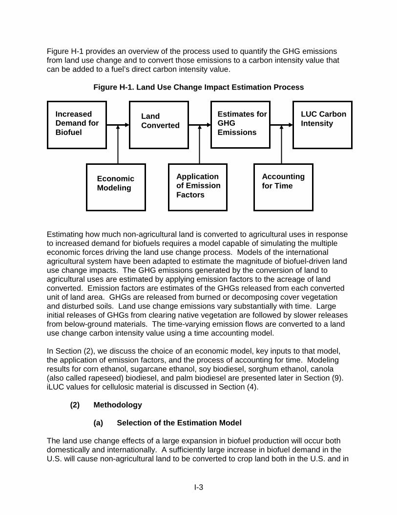
Figure H-1 provides an overview of the process used to quantify the GHG emissions from land use change and to convert those emissions to a carbon intensity value that can be added to a fuel’s direct carbon intensity value.
Figure H-1. Land Use Change Impact Estimation Process
Estimating how much non-agricultural land is converted to agricultural uses in response to increased demand for biofuels requires a model capable of simulating the multiple economic forces driving the land use change process. Models of the international agricultural system have been adapted to estimate the magnitude of biofuel-driven land use change impacts. The GHG emissions generated by the conversion of land to agricultural uses are estimated by applying emission factors to the acreage of land converted. Emission factors are estimates of the GHGs released from each converted unit of land area. GHGs are released from burned or decomposing cover vegetation and disturbed soils. Land use change emissions vary substantially with time. Large initial releases of GHGs from clearing native vegetation are followed by slower releases from below-ground materials. The time-varying emission flows are converted to a land use change carbon intensity value using a time accounting model. In Section (2), we discuss the choice of an economic model, key inputs to that model, the application of emission factors, and the process of accounting for time. Modeling results for corn ethanol, sugarcane ethanol, soy biodiesel, sorghum ethanol, canola (also called rapeseed) biodiesel, and palm biodiesel are presented later in Section (9). iLUC values for cellulosic material is discussed in Section (4).
(2) Methodology
(a) Selection of the Estimation Model The land use change effects of a large expansion in biofuel production will occur both domestically and internationally. A sufficiently large increase in biofuel demand in the U.S. will cause non-agricultural land to be converted to crop land both in the U.S. and in
Economic Modeling
Application of Emission Factors
Accounting for Time
LUC Carbon Intensity
Increased Demand for Biofuel
Land Converted
Estimates for GHG Emissions
I-3
countries with agricultural trade relations with the U.S. Models used to estimate land use change impacts must, therefore, be international in scope. In cooperation with researchers from UCB, ARB staff considered several models to estimate iLUC effects from biofuels. For the 2009 analysis, staff selected the GTAP model for iLUC analysis. The GTAP is a CGE model developed and supported by researchers at Purdue University. The GTAP has a global scope, is publicly available, and has a long history of use in modeling complex international economic effects. Therefore, ARB staff determined that the GTAP was the most suitable model for estimating the land use change impacts of the crop based biofuels that will be regulated under the LCFS. The GTAP is relatively mature, having been frequently tested on large-scale economic and policy issues. It has been used to assess the impacts of a variety of international economic initiatives, dating back to the Uruguay and Doha Rounds of the World Trade Organization’s General Agreement on Tariffs and Trade.2 It has been used to examine the expansion of the European Union, regional trade agreements, and multi-national climate change accords. A detailed discussion of the indirect land use change model selection process is provided in Appendix C of the 2009 ISOR at http://www.arb.ca.gov/regact/2009/lcfs09/lcfsisor2.pdf For the analysis approved by the Board in 2009, the GTAP model was modified by adding land use data on 18 worldwide agro-ecological zones, a carbon emissions factor table, and a co-products table (which adjusts GHG emission impacts based on the market displacement effects of co-products such as the dried distillers’ grains with solubles – a co-product of the ethanol production process). This model was termed GTAP-BIO. Predicted land use change impacts were aggregated by affected land use type (forest and pasture).
(b) Expert Working Group At the LCFS Hearing in 2009, stakeholders, in person and through written comments, expressed concerns related to the use of iLUC emissions, indicating that land use change was a new concept and not all of the scientific community had embraced the inclusion of this aspect in the life cycle analysis of transportation fuels. To accommodate such concerns, the Board, using Resolution 09-31, directed the Executive Officer to convene an Expert Workgroup (EWG) to assist the Board in refining and improving the land use and indirect effect analysis of transportation fuels. This workgroup was tasked with evaluating key factors that might impact the land use values for biofuels including agricultural yield improvements, co-product credits, land emission factors, food price elasticity, and other relevant factors. An Expert Workgroup was established in February 2010. The workgroup was comprised of 30 members, including eight representatives of other agencies involved in LCFS-type activities. Technical expertise to tackle major issues of concern was a key consideration in the selection of members. The individuals invited to participate in the Expert Workgroup were world-class specialists and represented a breadth of experience
2 The Uruguay Round began in September of 1986 and concluded in April, 1994. The Doha Round began in November of 2001 and is ongoing.
in their respective disciplines. The selected individuals came from diverse stakeholder groups such as government agencies, academic institutes and national laboratories, the biofuel and oil industries, and environmental groups. The membership list can be accessed at http://www.arb.ca.gov/fuels/lcfs/workgroups/ewg/ewg-members-list.pdf. Eight meetings of the Expert Workgroup were conducted in 2010. Several technical experts, who were either invited by the subgroups or by ARB staff, also presented during these meetings of the Expert Working Group. Meeting minutes and documents presented or discussed at these meetings were posted for public availability at the Expert Workgroup web site (http://www.arb.ca.gov/fuels/lcfs/workgroups/ewg/expertworkgroup.htm). Nine working subgroups were formed with each subgroup focusing on one of the following topical areas:
• Elasticity Values,
• Co-Product Credits,
• Land Cover Types,
• Uncertainty in Land Use Change Estimates,
• Indirect Effects of Fuels Other than Biofuels,
• Carbon Emission Factors,
• Time Accounting,
• Comparative and Alternative Modeling Approaches, and
• Food consumption effects. Each subgroup developed a work plan, deliberated on issues presented to them, and each subgroup presented their final recommendations in November 2010. In reports submitted to ARB, the subgroups were asked to summarize their recommendations in three categories: 1) near-term analysis, 2) short-term work/research, and 3) long-term work/research. ARB staff also contracted with two independent experts, Professor John Reilly, Co-Director of the Joint Program on the Science and Policy of Global Change at MIT Sloan, and Professor Steve Berry, James Burrows Moffatt Professor of Economics at Yale University. They were contracted to review changes made by Purdue University to the GTAP model through 2010 and also to provide feedback on iLUC approach used by staff. Professor Reilly performed a “top down” assessment of land use change modeling approaches and the GTAP modeling structure. Professor Berry performed a “bottom up” assessment of the model inputs to GTAP and the empirical basis for these inputs. In September 2010, both independent reviewers presented initial findings to the Expert Workgroup and in November the same year, delivered written reports to ARB
staff. All reports related to the EWG and the two independent experts can be accessed at http://www.arb.ca.gov/fuels/lcfs/workgroups/ewg/expertworkgroup.htm. The recommendations of the EWG combined with areas that staff deemed critical was presented to the Board at a Hearing in December 2010.
(c) Details of Updates to GTAP-BIO Model
ARB staff conducted a review of recommendations from the subgroups and independent reviewers to determine which recommendations were appropriate and could be completed in a timely manner for this round of model revisions. Recommendations not included in this round of revisions may be addressed as part of longer-term model updates. For several issues, disagreement over the recommended course of action existed between Expert Workgroup members or between Expert Workgroup members and the independent experts. In these situations, staff carefully weighed the evidence and consulted further prior to deciding on a course of action. Both ARB staff and Purdue researchers received additional information and comments from stakeholders and subject matter experts after the completion of the Expert Workgroup process. Staff, working with Purdue University, implemented many of the recommendations of the EWG. To accommodate stakeholder feedback, staff made additional modifications to refine the iLUC analysis using the GTAP-BIO model. Details of some of the refinements are available from publications by Taheripour et al.3,4 Specific model and iLUC analysis updates in the current revised modeling include:
• Use of the GTAP 7 database and baseline data for 2004 (2009 analysis used a 2001 baseline),
• Addition of cropland pasture in the U.S. and Brazil,
• Re-estimated energy sector demand and supply elasticity values,
• Improved treatment of corn ethanol co-product (DDGS),
• Improved treatment of soy meal, soy oil, and soy biodiesel,
• Modified structure of the livestock sector,
• Improved method of estimating the productivity of new cropland,
• More comprehensive and spatially explicit set of emission factors that are outside of the GTAP-BIO model,
3 Tyner, W., F. Taheripour, Q. Zhuang, D. Birur, and U. Baldos, July 2010: Land Use Changes and Consequent CO2 Emissions due to US Corn Ethanol Production: A Comprehensive Analysis, Revised Final Report, Department of Agricultural Economics, Purdue University. 4 Tyner, W., October 2011, Interim Report: Calculation of Indirect Land Use Change (ILUC) Values for Low Carbon Fuel Standard (LCFS) Fuel Pathways, posted online at https://www.gtap.agecon.purdue.edu/resources/download/5629.pdf
• Increased flexibility of crop switching in response to price signals,
• Incorporation of an endogenous yield adjustment for cropland pasture,
• Disaggregated sorghum from the coarse grains sector to allow for modeling iLUC
impacts for sorghum ethanol,
• Disaggregated canola (rapeseed) from the oilseeds sector to facilitate modeling of iLUC for canola based biodiesel,
• Included data for palm in the oilseeds sector to estimate iLUC for palm derived biodiesel,
• Developed regionalized land transformation elasticities for the model using recent evidence for land transformation5,
• Split crop production into irrigated versus rain-fed and develop datasets and metrics to assess impacts related to water-constraints in agriculture across the world. Details of the modeling efforts to include irrigation in the GTAP-BIO model is included in a report by Taheriour et al.6 Determining regions of the world where water constraints could limit expansion of irrigation was developed by researchers at the World Resources Institute (WRI) and is detailed in reports published by WRI7,8, and
• Disaggregated Yield Price Elasticity (YPE) parameter into regionalized and crop-specific values. For the current analysis, however, the same YPE value is used for all regions and crops9.
5 Taheripour, F., and Tyner, W. Biofuels and Land Use Change: Applying Recent Evidence to Model estimates, Appl. Sci. 2013, 3, 14-38 6 F. Taheripour, T. Hertel, and J. Liu, The role of irrigation in determining the global land use impacts of biofuels, Energy, Sustainability, and Society, 3:4, 2013, http://www.energsustainsoc.com/content/3/1/4 7 F. Gassert, M. Luck, M. Landis, P. Reig, and T. Shiao, Aqueduct Global Maps 2.1: Constructing Decision-Relevant Global Water Risk Indicators, Working Paper, World Resources Institute, April 2014. 8 F. Gassert, P. Reig, T. Luo, and A. Maddocks, A weighted aggregation of spatially distinct hydrological indicators, Working Paper, World Resources Institute, December 2013. 9 Staff conducted scenario runs using different values of YPE. For each run, YPE was the same across all regions and crops.
I-7
(d) Key Inputs to GTAP The primary input to computable general equilibrium models such as GTAP is the specification of the changes that will, by moving the economy away from equilibrium, result in the establishment of a new equilibrium. Parameters, such as elasticities, are used to estimate the extent which introduced changes alter the prior equilibrium. Listed below are the inputs and parameters that the GTAP uses to model the land use change impacts of increased biofuel production levels. Also listed are some of the important approaches used by staff for the current analysis.
• Baseline year: GTAP employs the 200410 world economic database as the analytical baseline. This is the most recent year for which a complete global land use database exists.
• Fuel production increase: The primary input to computable general equilibrium models such as GTAP is the specification of the changes that will result in a new equilibrium. “Shock’ corresponds to an increase in the volume of biofuel production used as an input to the model to estimate land use changes. For example, in Table H-1, for corn ethanol, the shock is 11.59 billion gallons and corresponds to the volume of corn ethanol being modeled to estimate iLUC emissions for this biofuel. Table H-1 lists the ’shocks’ used for all biofuels for which iLUC analysis was completed.
Table H-1. Shocks Used to Model Biofuel iLUC Emissions
• Yield Price elasticity (YPE): This parameter determines how much the crop yield
will increase in response to a price increase for the crop. Agricultural crop land is more intensively managed for higher priced crops. If the crop yield elasticity is 0.25, a P percent increase in the price of the crop relative to input cost will result in a percentage increase in crop yields equal to P times 0.25. The higher the elasticity, the greater the yield increases in response to a price increase. For the 2009 modeling, ARB used a yield-price elasticity value range of 0.2 to 0.6. Purdue researchers have used a single YPE value of 0.25 based on an
10 For the 2009 regulation, the baseline year was 2001.
I-8
econometric estimate made by Keeney and Hertel.11 The Keeney-Hertel estimate of 0.25 is obtained by averaging two values (0.28 and 0.24) from Houck and Gallagher,12 a value from Lyons and Thompson13 (0.22) and a value from Choi and Helmberger14 (0.27). An expert from UC Davis, contracted to conduct a review and statistical analysis of data from a few published studies also concluded that YPE values were small to zero. Staff conducted a comprehensive review of all available data and reports on YPE and concluded that YPE values were likely small. However, to account for the different values of YPE from recent studies combined with recommendations from the EWG, for the current analysis, staff has used values of YPE between 0.05 and 0.35. Details of the review conducted by staff on YPE is provided in Attachment 1.
• Elasticity of crop yields with respect to area expansion (ETA): This parameter
expresses the yields that will be realized from newly converted lands relative to yields on acreage previously devoted to that crop. Because almost all of the land that is well-suited to crop production has already been converted to agricultural uses, yields on newly converted lands are almost always lower than corresponding yields on existing crop lands. For the 2009 regulation, the scenario runs utilized a value of 0.25 and 0.75 for this parameter, based on empirical evidence from U. S. land use and expert judgment on the productivity of the new cropland. For the current analysis, Purdue University used results from the Terrestrial Ecosystem Model (TEM) to derive estimates of net primary productivity (NPP), a measure of maximum biomass productivity. The ratio of NPP of new cropland to existing cropland was used to estimate ETA for a given region/AEZ and is detailed in Taheripour et al.15 ETA values used in the current analysis are provided in Table H-2.
11 Keeney, R., and T. W. Hertel. 2008. “The Indirect Land Use Impacts of U.S. Biofuel Policies: The Importance of Acreage, Yield, and Bilateral Trade Responses.” GTAP Working Paper No. 52, Center for Global Trade Analysis, Purdue University, West Lafayette, IN. 12 Houck, J.P., and P.W. Gallagher. 1976. “The Price Responsiveness of U.S. Corn Yields.” American Journal of Agricultural Economics 58:731–34. 13 Lyons, D.C., and R.L. Thompson. 1981. “The Effect of Distortions in Relative Prices on Corn Productivity and Exports: A Cross-Country Study.” Journal of Rural Development 4:83– 102. 14 Choi, J.S., and P.G. Helmberger. 1993. “How Sensitive are Crop Yield to Price Changes and Farm Programs?” Journal of Agricultural and Applied Economics 25:237–44. 15 F. Taheripour, Q. Zhuang, W. Tyner, and X. Lu, Biofuels, Cropland Expansion, and the Extensive Margin, Energy, Sustainability, and Society, 2:25, 2012, http://www.energsustainsoc.com/content/2/1/25
I-9
Table H-2. Baseline ETA Values for Each Region/AEZ
• Elasticity of land transformation across cropland, pasture and forest land (ETL):
This elasticity expresses the extent to which expansion into forestland and pastureland occurs due to increased demand for agricultural land (driven by higher crop prices). This is implemented in the model using a land transformation elasticity parameter labeled ETL1. For the 2009 analysis, a range of 0.1 to 0.3 was used for this parameter. Purdue University,5 utilizing data for land conversion in the 2000-2012 timeframe modified this elasticity and segregated ETL1 into ETL11 and ETL12. The modified tree structure is shown in Figure H-2. Minor modifications to published values were made to the ARB version of the GTAP-BIO model by Purdue University and these are provided in the Section (9).
I-10
Figure H-2. Modified Land Transformation Tree Structure
• Elasticity of harvested acreage response: This parameter expresses the extent to which changes occur in cropping patterns of existing agricultural land as land costs change. The higher the value, the more cropping patterns will change (e.g. soybean to corn) in response to land costs. This is implemented using an elasticity of land transformation parameter labeled ETL2. The modified tree structure is shown in Figure H-2. For the 2009 analysis, the model used a single value for this parameter and the value used was 0.5. For the current analysis, each region in the model has a different value of ETL2 and these are detailed in Taheripour et al.5 The disaggregation of cropland into irrigated and rain-fed necessitated the incorporation of additional elasticities, labeled ETL4 and ETL5 to account for land transformations in the irrigated crop and rain-fed crop land categories respectively. For the present analysis, using Purdue University’s recommendation, staff chose to use the ETL2 values for ETL4 and ETL5 for each region within the model. Table H-3 lists the baseline ETL values used for the current analysis.
I-11
Table H-3. Land Transformation Elasticities by Region
• Incorporation of an endogenous yield adjustment for cropland pasture:
Cropland-pasture category was not available as a land category for the 2009 analysis. In the current analysis, cropland-pasture is used primarily as an input to the livestock industry. As cropland-pasture is converted to dedicated crop production in response to biofuel expansion, land rents will rise which may lead to investments by the land owner to increase productivity of the land. This potential response led researchers at Purdue University to define a module to link productivity of cropland-pasture with its rent through an elasticity parameter.16 However, Purdue researchers acknowledge that although they believe the effect is real, there is no empirical basis for the elasticity parameter proposed for this endogenous yield adjustment. In the absence of empirical evidence to estimate this parameter, staff used two sets of values for the runs employed for each biofuel analyzed here. The first set uses values of 0.1 for Brazil and 0.2 for the U.S. and the second set uses values of 0.2 for Brazil and 0.4 for the U. S.
16 Taheripour, F., W. Tyner, and M. Wang. August 2011. Global Land Use Changes due to the U.S. Cellulosic Biofuel Program Simulated with the GTAP Model
I-12
(e) Emission Factors related to Land Conversion and AEZ-EF Model
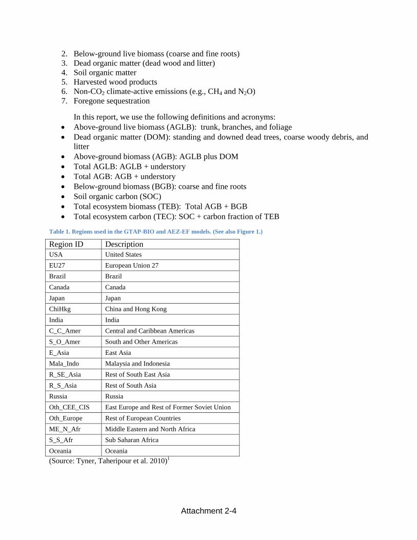
GTAP modeling provides an estimate for the amounts and types of land across the world that is converted to agricultural production as a result of the increased demand for biofuels. The land conversion estimates made by GTAP are disaggregated by world region and agro-ecological zones (AEZ). In total, there are 19 regions and 18 AEZs. The next step in calculating an estimate for GHG emissions resulting from land conversion is to apply a set of emission factors. Emission factors provide average values of emissions per unit land area for carbon stored above and below ground as well as the annual amount of carbon sequestered by native vegetation. The amount of “lost sequestration capacity” per unit land area results from the conversion of native vegetation to crops. For the 2009 regulation, staff used emission factor data from Searchinger et al. (2008)17. A spreadsheet detailing emission factors used for the LCFS in 2009 is located at http://www.arb.ca.gov/fuels/lcfs/ef_tables.xls. In the 2009 modeling, each of the 19 regions had separate emission factors for forest and pasture conversion to cropland but these emission factors did not vary by AEZ within each region. Because land conversion estimates within each region differ significantly by AEZ and both biomass and soil carbon stocks also vary significantly by AEZ, emission factors specific to each region/AEZ combination are appropriate. ARB contracted with researchers at UC Berkeley, University of Wisconsin-Madison, and UC Davis to develop the agro-ecological zone emission factor (AEZ-EF) model. The model combines matrices of carbon fluxes (MgCO2 ha-1 y-1) with matrices of changes in land use (ha) according to land-use category as projected by the GTAP-BIO model. As published, AEZ-EF aggregates the carbon flows to the same 19 regions and 18 AEZs used by GTAP-BIO. The AEZ-EF model contains separate carbon stock estimates (MgC ha-1) for biomass and soil carbon, indexed by GTAP AEZ and region, or “Region-AEZ”.18,19 The model combines these carbon stock data with assumptions about carbon loss from soils and biomass, mode of conversion (i.e., whether by fire), quantity and species of carbonaceous and other greenhouse gas (GHG) emissions resulting from conversion, carbon remaining in harvested wood products and char, and foregone sequestration. The model relies heavily on IPCC greenhouse gas inventory methods and default values (IPCC 200620), augmented with more detailed and recent data where available. Details of this model, originally published in 2011 is available in reports
17 This data set is referred to as the “Woods Hole” data because it was compiled by Searchinger’s co-author, R. A. Houghton, who is affiliated with the Woods Hole Oceanographic Institute. 18 Gibbs, H., S. Yui, and R. Plevin. (2014) “New Estimates of Soil and Biomass Carbon Stocks for Global Economic Models.” Global Trade Analysis Project (GTAP) Technical Paper No. 33. Center for Global Trade Analysis, Department of Agricultural Economics, Purdue University. West Lafayette, IN. 19 Plevin, R., H. Gibbs, J. Duffy, S. Yui and S. Yeh. (2014) “Agro-ecological Zone Emission Factor (AEZ-EF) Model (v47).” Global Trade Analysis Project (GTAP) Technical Paper No. 34. Center for Global Trade Analysis, Department of Agricultural Economics, Purdue University. West Lafayette, IN. 20 http://www.ipcc-nggip.iges.or.jp/public/2006gl/index.html
submitted to ARB by Holly Gibbs and Richard Plevin.21,22 In response to stakeholder feedback from workshops, this version was modified and the updates include:
1) Contributions to carbon emissions from Harvested Wood Products (HWP) was updated in the model using data compiled by Earles et al.23
2) Additional modifications to HWP were performed using above-ground live biomass (AGLB) after 30 years in each region
3) Peat emission factor was updated to 95 Mg CO2/ha/yr using the ICCT report24 4) Added OilPalmCarbonStock based on Winrock update to RFS2 analysis.25,26 5) Updated forest biomass carbon, forest area, and forest soil carbon data using
latest data from Gibbs et al.18 6) Updated IPCC_GRASSLAND_BIOMASS_TABLE with data from Gibbs et al.18
As discussed above, the conversion of forest, pasture, or cropland pasture to agricultural uses releases much of the carbon stored in these ecosystems. The releases happen over a period of years, as follows:
• An initial GHG burst from burning and/or decaying cover vegetation; this is referred to as the above ground release;
• A slower release of carbon from disturbed soils: larger emissions occur during the first few years, followed by declining releases. This process is referred to as the below-ground release; and
• Loss of the carbon sequestration capacity of the cleared vegetation. Figure H-3 shows a representative time-profile for emissions resulting from land use change assuming a project start date of 2010 and an end date of 2040. The above and below-ground emissions and foregone sequestration values used in these scenarios are for illustrative purposes only and are not final LCFS values. The land use change emissions profile depicted in Figure H-3 assumes that:
21 Gibbs, H. and S. Yui, September 2011. Preliminary Report: New Geographically-Explicit Estimates of Soil and Biomass Carbon Stocks by GTAP Region and AEZ, posted online at http://www.arb.ca.gov/fuels/lcfs/09142011_iluc_hgreport.pdf 22 Plevin, R., H. Gibbs, J. Duffy, S. Yui, and S. Yeh, September 2011. Preliminary Report: Agro-ecological Zone Emission Factor Model, posted online at http://www.arb.ca.gov/fuels/lcfs/09142011_aez_ef_model_v15.pdf 23 Earles J. M., Yeh, S., and Skog, K. E., Timing of carbon emissions from global forest clearance, Nature Climate Change, 2012; DOI: 10.1038/nclimate1535 24 Page, S. E., Morrison, R., Malins, C., Hooijer, A., Rieley, J. O., and Jauhiainen, J., Review of Peat Surface Greenhouse Gas Emissions from Oil Palm Plantations in Southeast Asia, White Paper Number 15, September 2011, www.theicct.org 25 Harris, N., and Grimland, S., 2011a. Spatial Modeling of Future Oil Palm Expansion in Indonesia, 2000 to 2022. Winrock International. Draft report submitted to EPA. 26 Harris, N., and Grimland, S., 2011b. Spatial Modeling of Future Oil Palm Expansion in Malaysia, 2003 to 2022. Winrock International. Draft report submitted to EPA.
• All above-ground carbon is released in year one due to burning of native vegetation to clear the land for cultivation;
• The majority of below-ground release occurs over the first five years followed by a much slower release over the next 15 years; and
• Forgone sequestration occurs over the entire project period.
Figure H-3. Representative Land Use Change Emissions Profile
Calculating the carbon intensity for a crop based biofuel (e.g. corn ethanol) requires that time-varying emissions be accounted for in a manner that allows meaningful comparison with the carbon intensity of a reference fuel (e.g. gasoline displaced by the biofuel) which releases greenhouse gases at a relatively constant rate over the years in which it is used. Staff chose to use a 30-year accounting timeframe for the LCFS in 2009 and has chosen to maintain the same one for this round of analysis. Additional details of time accounting and considerations for the 30-year selection is provided in Attachment 3. Averaging of carbon emissions over a 30-year timeframe has been used in the carbon emissions factor model. The AEZ-EF model documentation is available in Attachment 2. This document details all the sources of data, methodologies used to estimate carbon release, assumptions, etc. used in developing this model. The current version of the
0
100
200
300
400
500
2010 2015 2020 2025 2030 2035 2040 2045 2050 2055
Year
LUC
Em
issi
ons
(gC
O2e
/MJ
of a
nnua
l pr
oduc
tion)
Foregone sequestration
Below ground and foregone sequestration
Below ground and foregone sequestration
Above and below ground and foregone sequestration
I-15
AEZ-EF spreadsheet model (v. 52) and documentation are available from the LCFS web site at http://www.arb.ca.gov/fuels/lcfs/lcfs.htm.
(f) Integration of GTAP-BIO results with the AEZ-EF Model The outputs of the GTAP-BIO model include estimated land conversions (forest, pasture, and cropland-pasture) for each biofuel shock with the corresponding input values. The land conversions are generated by AEZ and regions within the GTAP-BIO model. The outputs from this model are then mapped to corresponding AEZ/Regions within the AEZ-EF model. This is shown in the schematic in Figure H-4. The combination of the two models generates total carbon emissions which are then normalized by the total fuel production (i.e., MJ of fuel produced) and averaged over 30 years to produce an iLUC value for each scenario run.
Figure H-4. Integration of the GTAP-BIO Model with the AEZ-EF Model
In the 2009 modeling effort, the iLUC value for each pathway was an average of multiple scenarios run with different input values for key parameters such as yield-price elasticity and productivity of newly converted cropland. Unfortunately, there was inconsistency between the number of scenarios run and the input parameters used for different fuel pathways. In this revised modeling the input values are the same across all pathways. Moreover, the iLUC carbon intensity values are based on an average of 30 scenarios with input parameters based on the best available data. Volumes of biofuels used in the modeling is shown in Table H-1. Details of the 30 scenario runs with the corresponding input values is provided in the Section (9).
(3) Uncertainty Analysis The EWG subgroup on uncertainty recommended staff to complete a comprehensive analysis of the impacts of uncertainty in input parameter values on iLUC values. Staff contracted with the University of California, Berkeley to develop a methodology to estimate impacts of uncertainty on iLUC emissions. The researchers proposed the use of a Monte Carlo Simulation (MCS) approach to evaluating uncertainty in iLUC analysis. They chose MCS because of the features below:
• The ability to represent arbitrary input and output distributions,
• The ability to perform global sensitivity analysis (e.g., contribution to variance) to identify which input parameters contribute most to the variance in the output, and
• The ability to represent parameter correlations. A primary disadvantage of Monte Carlo simulation historically has been the computational cost and time required. But with advances in computational technologies, Berkeley researchers were able to use resources at the National Energy Research Scientific Computing center’s massively parallel compute cluster and complete thousands of simulations required for MCS in just a few hours. The purpose of the Monte Carlo analysis is two-fold: 1) Identify the model parameters and parameter groups contributing most of the
variance to the resulting iLUC emissions value.
2) Characterize the output distribution for the iLUC emission value for various types of biofuel.
The iLUC Monte Carlo Simulator (iLUC-MCS) system developed by Berkeley combines together the two models GTAP-BIO and AEZ-EF and runs uncertainty simulations on a large-scale parallel computing system. Figure H-5 depicts how the MCS system integrates the two models together. Key model parameters within the GTAP-BIO and AEZ-EF models are described by probability distributions. Latin hyper cube sampling methodology27 was employed to generate a representative sample of parameter values from a multidimensional matrix of parameters used in the two models. These were used as inputs to the GTAP-BIO model, the outputs of which were used in the AEZ-EF model to generate discrete outputs for each of the inputs used for the MCS runs. The set of outputs describes a frequency distribution which details the variance in the output given the variance in the model inputs. For the initial runs, Monte Carlo analysis was used to identify the parameters that contribute the most to uncertainty. Once the critical parameters were identified, researchers at UC Berkeley and UC Davis consulted with
experts and reviewed literature to update probability distributions and ranges for the critical parameters. Subsequent simulations were performed by utilizing distributions and ranges only for the critical parameters. The output distributions for the iLUC values for all the 6 biofuels analyzed are provided in the Section (9). Details of the distributions and ranges used for the parameters in the Monte Carlo analysis is provided in Attachment 4.
Figure H-5. Representation of the GTAP-BIO and AEZ-EF in the MCS System
(4) Indirect Effects: Land Use Change Effects for Cellulosic Ethanol The current version of the GTAP-BIO model is not capable of estimating the land-use-change effects of plant-based feedstocks that do not displace agricultural commodities. To assess the land use change effects of cellulosic ethanol produced from such feedstocks, therefore, staff turned to an analysis prepared by Purdue University.28 This analysis evaluated the potential land use change impacts of corn stover, miscanthus, and switchgrass which can be used as feedstock for the production of cellulosic ethanol. Purdue’s results indicate that the use of corn stover, is unlikely to generate land use change impacts, it may actually yield benefits in the form of a reduction in the amount of land required for fuel crop cultivation. For switchgrass and miscanthus, however, the study concluded that there are land use change impacts from these crops but are likely
28 F. Taheripour, W. Tyner, and M. Wang, Global Land Use Changes due to the U.S. Cellulosic Biofuel Program Simulated with the GTAP Model, 2011 (greet.es.anl.gov/files/luc_ethanol)
I-18
to be significantly lower than those for feedstocks that displace food and feed crops. Staff is currently working to integrate the necessary datasets for this analysis into the GTAP model. Once these modifications have been made, staff will prepare and present the modeling results. For the current regulation, staff proposes to use the value of 18 gCO2/MJ for cellulosic feedstocks. This was the value used for the 2009 regulation. Staff is currently working with CEC, Purdue researchers, the U.S. EPA and others in determining appropriate inputs, values, etc. for cellulosic ethanol from non-food crops and waste. Results will be published when the analyses are completed. (5) Land Use Impacts from Crude Production in California As with biofuels production, producing fossil fuels from a new crude source will likely result in carbon releases from disturbed land. Staff in association with academics at Stanford University developed the OPGEE model to estimate GHG emissions from crude production. This model includes estimates of GHG emissions from land use change attributable to production of crude in various regions of the world. Details are available in published documentation.29 Appropriate values of land use change are included in the CI calculations for based on the location of crude production for all the different crudes that come to California. (6) Additional Aspects in iLUC Analysis
(a) Comparison of GTAP-BIO Results with Observed Market Behavior
The GTAP-BIO is designed to project the specific effects of one carefully defined policy change—namely the increased production of a biofuel. Because it focuses narrowly on a specific set of economic changes, the results obtained from GTAP-BIO will not necessarily reflect observed aggregate trends. The model predicts, for example, that the expanded use of domestic corn for the production of ethanol will reduce U.S. corn exports. That prediction appears to be inconsistent with some actual trade data. Those data show that the production of corn, soybeans and wheat in the United States has generally been on the increase over the last decade. Exports meanwhile have remained relatively steady. In the case of corn, production increases have been sufficient to supply the ethanol industry while maintaining export levels. The effects of increased biofuel production on export markets are masked by other phenomena that are not addressed by the GTAP analysis. In recent years there appears to have been an increase in the demand for American agricultural products in rapidly growing economies such as China. A significant component of the increased demand in China and other rapidly developing countries is a sharp increase in the consumption of meat and soy products in those countries. This has created a demand for imported soybeans and corn, which are used as livestock
29 Oil Production Greenhouse Gas Emissions Estimator OPGEE v1.1 Draft D User guide and Technical documentation.
I-19
feed. This demand has helped to increase prices and has kept U.S. exports steady, despite the rapidly increasing use of corn for the production of ethanol. The increased demand for corn ethanol, along with strong corn export demand, stimulated a significant increase in corn production over the 2005 through 2012 period. This expansion in corn production coincided with significant decline in soybean production. When U.S. corn acreage is expanded, the crop that is most often displaced is soybeans. The overall trend in corn exports, therefore, is the result of many factors, only one of which is the growth in corn ethanol production. Because the observed trend is the net result of several factors, the independent influence of increased ethanol production was masked by competing influences not considered in the GTAP results. It is true, however, that the downward pressure from domestic ethanol production kept exports lower than they would otherwise have been. The GTAP-BIO analysis was designed to isolate the incremental contribution of ethanol production to export levels. Other influences, which can mask the effects of ethanol production, are not included in the model. It is important to keep this fact in mind when evaluating GTAP-BIO projections in the context of observed market behavior. GTAP-BIO is not predicting the overall aggregate market trend—only the incremental contribution of a single factor to that trend. If GTAP-BIO projects reduced exports, for example, this should be understood to mean that exports will be lower than what they would have been in the absence of the effect being modeled (increased ethanol production, in this case). It is the difference between predicting an absolute change and a relative change. GTAP-BIO projections are incremental and relative.
(b) Location of Land Use Changes The GTAP-BIO model is designed to respond to changed economic conditions by solving for the most economically efficient new equilibrium point. In response to a 11.59 billion gallon increase in the demand for corn ethanol, as well as the other biofuels evaluated, the model seeks the least-cost source of the biofuel feedstocks needed to sustain that demand. Although some additional feedstocks can be obtained through higher yields, the overall demand cannot be met unless the number of acres devoted to corn production can be expanded significantly. When additional acreage is needed, American farmers are most likely to convert one cropland to another and bring new land into productivity. This is especially true when returns from exports are high, as they have been until very recently. If returns from exports are low, more of the demand for corn would be met through reduced exports, driving a greater proportion of the land use change impact overseas to America’s trading partners. For example, reduced soybean supplies increase soybean prices, stimulating the demand for more land to support soybean production. If soybean exports have remained high, much of the demand for soybean acreage will be met domestically. Soybeans can be grown on land previously devoted to other crops, such as wheat, but, some of the displaced soybeans, wheat, and other crops must be grown on land that was not previously under cultivation. This is the source of the domestic land use change impact identified by GTAP-BIO.
I-20
The GTAP-BIO brings new land into agricultural production from forest and grassland areas. It isn’t specific about exactly where that land will come from. Some could come from the Conservation Reserve Program (CRP). Most CRP lands are in the arid far west and could support soybean production but not corn. Although the penalties for breaking CRP contracts are steep enough to prevent CRP lands from being used before their contracts expire, contracts are currently expiring on two million acres due to provisions contained in the recent Farm Bill. The USDA has the authority to make additional CRP lands available. If sufficient CRP land is not available to indirectly support an expansion of corn acreage, a large supply of non-CRP pasture land that was formerly in crops could be brought back into production. The GTAP modelers assumed that no CRP land would be converted in response to increased biofuel demand. Although some CRP land has been released for cultivation, an abundance of previously farmed pasture land is also available. These pasture lands are generally more productive than the lands released from the CRP system. Before it becomes economical to convert the least productive domestic land areas, land use change tended to shift overseas.
(c) Food Versus Fuel Analysis The LCFS, together with biofuel production mandates in the U.S. and Europe, will result in the diversion of agricultural land from food production to biofuel feedstock production. This diversion of agricultural land to biofuel production will exert an upward pressure on food commodity prices, and potentially lead to food shortages, increasing food price volatility, and inability of the world’s poorest people to purchase adequate quantities of food. 30,31 GTAP analysis predicts that price increases resulting from the additional demand for biofuels will result in reduced crop production, leading to lower food consumption. Some stakeholders maintain that global changes in food consumption are not a direct consequence of biofuel production and staff should not consider food impacts in the modeling of iLUC while others argue that reductions in food consumption would require an assessment of the calorific content of finished food products in the GTAP-BIO model. The model as currently structured, is not capable of modeling any changes in food consumption driven by calorific content. Staff is therefore, proposing to address this issue in future updates. (7) Long Term Updates to iLUC analysis The EWG tagged several recommendations under long-term updates to the model. These have not been included in the current analysis for the re-adoption of the LCFS regulation. At workshops and through email correspondence, stakeholders have submitted feedback to staff to refine the current iLUC analysis. In addition, a comprehensive review by staff of the structure, input values, parameters etc. within the
30 Sustainable Bioenergy: A Framework for Decision Makers: United Nations Energy (2007). 31 D. J. Tenenbaum , “Food vs. Fuel: Diversion of Crops Could Cause More Hunger.”, Environmental Perepectives 116(6): A254-257, (2008).
I-21
model has identified areas that need improvement. Staff, is therefore, proposing to consider these together with the recommendations by the EWG and stakeholders and refine the iLUC analysis in the future. The specific areas include:
1) The inclusion of land under the Conservation Reserve Program; 2) The use of improved emission factors, as they become available; 3) The evaluation and possible use of data and analyses provided by stakeholders; 4) Consider the disaggregation of the forest category into unmanaged and
managed (for timber production) forests. 5) Characterizing in greater detail of the land use types that are subject to
conversion by the GTAP model (forest, grassland, CRP, idle and fallow croplands, etc.).
6) Account for the impacts from fertilizer, livestock, and paddy rice emissions. The EWG had recommended the inclusion of such effects.32
7) Consider accounting for the effects of non-Kyoto climate forcing gases and particles (e.g., black carbon) in addition to carbon dioxide, methane, and nitrous oxide.33
8) Adopt a modeling framework that allows for the dynamic nature of land use change that can incorporate time dependent changes such as technology driven yield improvements and food demand (influenced by the dynamics of economic and demographic change). This will likely involve switching to a dynamic version of GTAP.34
9) Evaluate alternative approaches to calculating yields on new agricultural lands based on statistical analysis of climate and management factors using updated datasets.35 Estimates of yields on newly converted lands should also factor in economics of land selection.36
10) Evaluate alternative approaches to how the model determines which land types (e.g., forest or pasture lands) are converted to cropland. This either involves a significant change in model structure or the use of land conversion probabilities for each region of the world which are exogenous to the model. The current structure used by Purdue needs refinement in the values of elasticity of land transformation for all regions within the model. Alternatively, the model could be used to predict only the amount of land converted and observed data for land conversion probabilities could be used to estimate the type of land converted.37,38
11) Evaluate the use of Armington versus Heckschler-Ohlin structures for modeling international trade. The use of Armington structure for trade in GTAP, although
32 Carbon Emission Factors Subgroup, Final Report to the LCFS Expert Workgroup, November 19, 2010 posted online at http://www.arb.ca.gov/fuels/lcfs/workgroups/ewg/expertworkgroup.htm 33 Ibid. 34 Land Cover Types Subgroup, Final Report to the LCFS Expert Workgroup, November 22, 2010 posted online at http://www.arb.ca.gov/fuels/lcfs/workgroups/ewg/expertworkgroup.htm 35 Ibid. 36 Berry, S., January 4, 2011. Report to ARB: Biofuels Policy and the Empirical Inputs to GTAP Models. Posted online at http://www.arb.ca.gov/fuels/lcfs/workgroups/ewg/expertworkgroup.htm 37 Ibid. 38 Elasticity Values Subgroup, Final Report to the LCFS Expert Workgroup, 2010, posted online at http://www.arb.ca.gov/fuels/lcfs/workgroups/ewg/expertworkgroup.htm
appropriate in the short term, may be unrealistic over the long term. Armington assumptions give greater preference to meeting increased demand with domestic production or from normal trading partners. In contrast, the Heckschler-Ohlin structure assumes similar crops of different origin are nearly perfect substitutes.39,40
12) Evaluation and development of methodology to account for multiple cropping (i.e., double-cropping, triple-cropping, etc.).
13) Refinement of cropland pasture elasticity (PAEL). 14) Refine extensification/intensification in the model based on available information. 15) Re-evaluate yield price elasticity based on new data.
In addition to these, additional refinements could be considered based on published literature, studies, and reports that become available in the future. (8) Other Indirect Effects Staff has identified no other significant effects that result in large GHG emissions that would substantially affect the LCFS framework for reducing the carbon intensity of transportation fuels. In addition, stakeholders have not provided any quantitative analysis that demonstrates that these impacts are significant. Providers of crop-based biofuels continue to maintain, however, that significant market-mediated indirect effects other than land use change are likely to exist. Staff will continue to work with interested parties to identify and measure such effects. (9) Results of iLUC analysis with the GTAP-BIO and AEZ-EF Models For the current regulatory process, staff has completed iLUC analysis for 6 biofuels and they include:
• Corn Ethanol
• Sugarcane Ethanol
• Soy Biodiesel
• Canola Biodiesel (also Rapeseed Biodiesel)
• Sorghum Ethanol
• Palm Biodiesel
39 Berry, S., January 4, 2011. Report to ARB: Biofuels Policy and the Empirical Inputs to GTAP Models. Posted online at http://www.arb.ca.gov/fuels/lcfs/workgroups/ewg/expertworkgroup.htm 40 Reilly, J., November 4, 2010, Report to ARB: GTAP-BIO-ADV and Land Use Emissions from Expanded Biofuels Production, Posted online at http://www.arb.ca.gov/fuels/lcfs/workgroups/ewg/expertworkgroup.htm
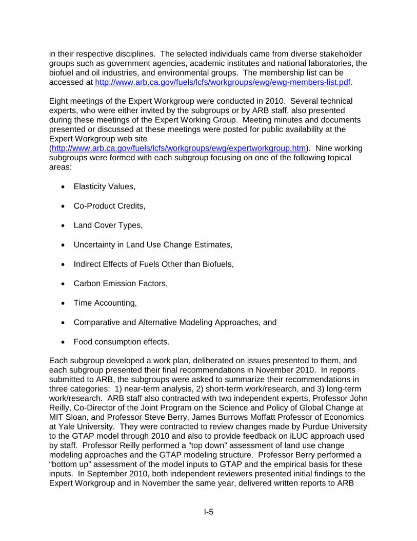
Table H-1 lists production levels (shocks) utilized in modeling iLUC emissions for the biofuels analyzed here. The iLUC results were estimated as an average of 30 scenario runs, conducted by varying critical parameters that have the largest impacts on model outputs. Table H-4 provides details of the 30 scenario runs with input parameter values used for each of biofuel analyzed for this regulation.
Table H-4. Summary of Scenario Parameter Values
Scenario YPE PAEL_BR PAEL_US TEM 1 0.05 0.1 0.2 Baseline TEM 2 0.05 0.2 0.4 Baseline TEM 3 0.1 0.1 0.2 Baseline TEM 4 0.1 0.2 0.4 Baseline TEM 5 0.175 0.1 0.2 Baseline TEM 6 0.175 0.2 0.4 Baseline TEM 7 0.25 0.1 0.2 Baseline TEM 8 0.25 0.2 0.4 Baseline TEM 9 0.35 0.1 0.2 Baseline TEM
10 0.35 0.2 0.4 Baseline TEM 11 0.05 0.1 0.2 120% TEM Baseline 12 0.05 0.2 0.4 120% TEM Baseline 13 0.1 0.1 0.2 120% TEM Baseline 14 0.1 0.2 0.4 120% TEM Baseline 15 0.175 0.1 0.2 120% TEM Baseline 16 0.175 0.2 0.4 120% TEM Baseline 17 0.25 0.1 0.2 120% TEM Baseline 18 0.25 0.2 0.4 120% TEM Baseline 19 0.35 0.1 0.2 120% TEM Baseline 20 0.35 0.2 0.4 120% TEM Baseline 21 0.05 0.1 0.2 80% TEM Baseline 22 0.05 0.2 0.4 80% TEM Baseline 23 0.1 0.1 0.2 80% TEM Baseline 24 0.1 0.2 0.4 80% TEM Baseline 25 0.175 0.1 0.2 80% TEM Baseline 26 0.175 0.2 0.4 80% TEM Baseline 27 0.25 0.1 0.2 80% TEM Baseline 28 0.25 0.2 0.4 80% TEM Baseline 29 0.35 0.1 0.2 80% TEM Baseline 30 0.35 0.2 0.4 80% TEM Baseline
I-24
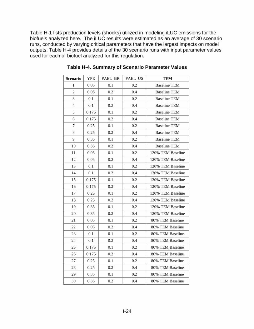
Table H-5 summarizes the iLUC values for all the 6 biofuels analyzed for the LCFS regulation. The values are the average of 30 scenario runs for each biofuel. Complete details for each of the biofuels are also provided in this section.
Table H-5. Summary of iLUC Values
Biofuel iLUC (gCO2/MJ)
Corn Ethanol 19.8
Sugarcane Ethanol 11.8
Soy Biodiesel 29.1
Canola Biodiesel 19.4
Sorghum Ethanol 14.5
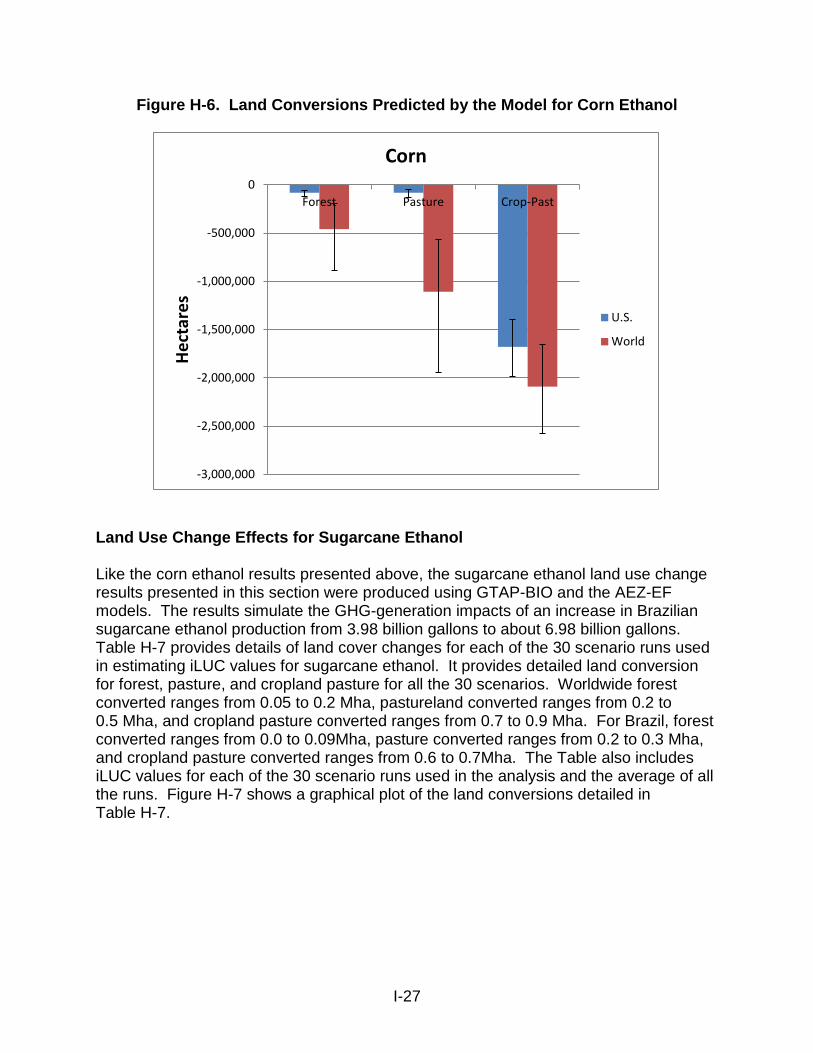
Palm Biodiesel 71.4 Land Use Change Effects for Corn Ethanol The corn ethanol land use change results presented in this section were generated using the GTAP-BIO and AEZ-EF models described earlier. An ethanol production increase of 11.59 billion gallons was assumed for all the modeling runs. This production increment corresponds to increasing U.S. corn ethanol production from 3.41 billion gallons produced in 2004 to the 15 billion gallon volume authorized by the Energy Independence and Security Act of 2007 (EISA). Table H-6 provides details of land cover changes for each of the 30 scenario runs used in estimating iLUC values for corn ethanol. It provides detailed land conversion for forest, pasture, and cropland pasture for all the 30 scenarios. Worldwide forest converted ranges from 0.2 to 0.9 Mha, pasture converted ranges from 0.6 to 1.9 Mha, and cropland pasture converted ranges from 1.7 to 2.5 Mha. For the United States, forest converted ranges from 0.06 to 0.1 Mha, pasture converted ranges from 0.05 to 0.2 Mha, and cropland pasture converted ranges from 1.4 to 1.9 Mha. The Table also includes iLUC values for each of the 30 scenario runs used in the analysis and the average of all the runs. Figure H-6 shows a graphical plot of the land conversions detailed in Table H-6.
I-25
Table H-6. Estimates of Land Converted Predicted and iLUC Results for the 30 Scenario Runs for Corn Ethanol
Scenario World-Wide Land Converted (ha) Land Converted in the U. S. (ha) iLUC
Figure H-6. Land Conversions Predicted by the Model for Corn Ethanol
Land Use Change Effects for Sugarcane Ethanol Like the corn ethanol results presented above, the sugarcane ethanol land use change results presented in this section were produced using GTAP-BIO and the AEZ-EF models. The results simulate the GHG-generation impacts of an increase in Brazilian sugarcane ethanol production from 3.98 billion gallons to about 6.98 billion gallons. Table H-7 provides details of land cover changes for each of the 30 scenario runs used in estimating iLUC values for sugarcane ethanol. It provides detailed land conversion for forest, pasture, and cropland pasture for all the 30 scenarios. Worldwide forest converted ranges from 0.05 to 0.2 Mha, pastureland converted ranges from 0.2 to 0.5 Mha, and cropland pasture converted ranges from 0.7 to 0.9 Mha. For Brazil, forest converted ranges from 0.0 to 0.09Mha, pasture converted ranges from 0.2 to 0.3 Mha, and cropland pasture converted ranges from 0.6 to 0.7Mha. The Table also includes iLUC values for each of the 30 scenario runs used in the analysis and the average of all the runs. Figure H-7 shows a graphical plot of the land conversions detailed in Table H-7.
-3,000,000
-2,500,000
-2,000,000
-1,500,000
-1,000,000
-500,000
0Forest Pasture Crop-Past
Hec
tare
s Corn
U.S.
World
I-27
Table H-7. Estimates of Land Converted Predicted and iLUC Results for the 30 Scenario Runs for Sugarcane Ethanol
Scenario World-Wide Land Converted (ha) Land Converted in Brazil (ha) iLUC
Figure H-7. Land Conversions Predicted by the Model for Sugarcane Ethanol
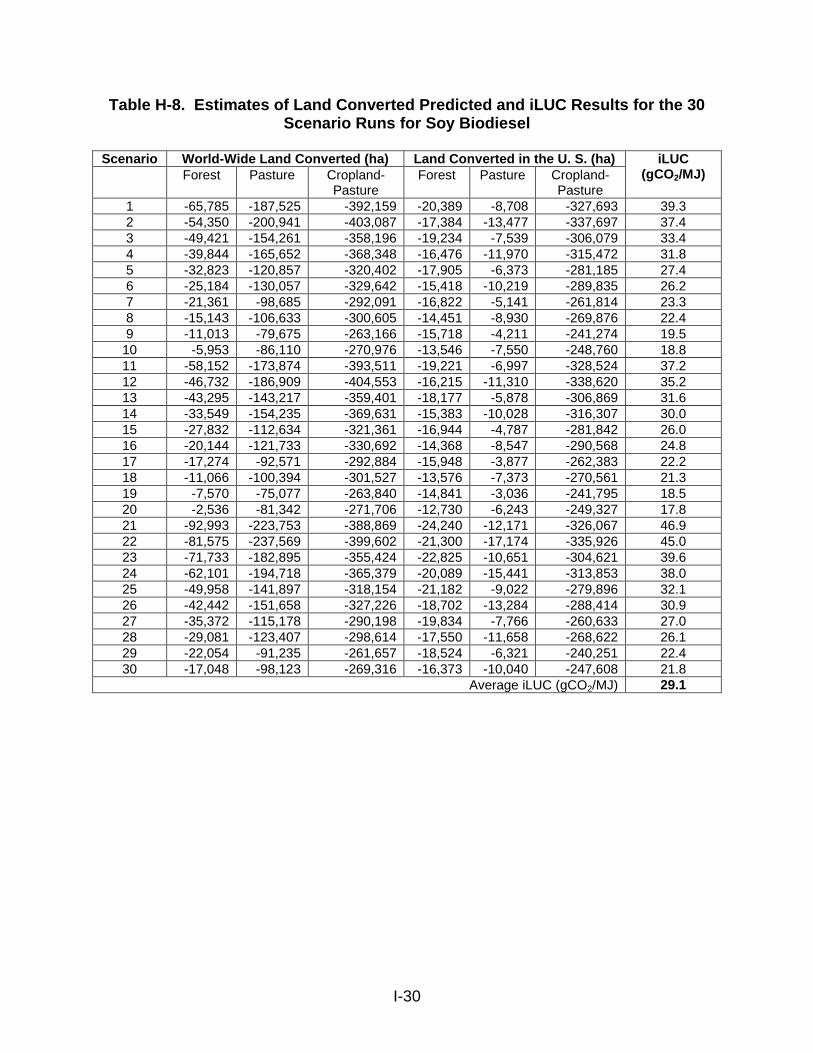
Land Use Change Effects for Soy Biodiesel Like the corn ethanol and sugarcane ethanol results presented above, the soy biodiesel land use change results presented in this section were produced using GTAP-BIO and the AEZ-EF models. Starting with the 2004 U.S. soy biodiesel production level of 0.024 billion gallons, staff analysis used 0.812 billion gallons of soy biodiesel shock for a total of 0.836 billion gallons of U.S. soy biodiesel. Table H-8 provides details of land cover changes for each of the 30 scenario runs used in estimating iLUC values for soy biodiesel. It provides detailed land conversion for forest, pasture, and cropland pasture for all the 30 scenarios. Worldwide forest converted ranges from 0.00 to 0.09 Mha, pasture converted ranges from 0.07 to 0.2 Mha, and cropland pasture converted ranges from 0.3 to 0.4 Mha. For the United States, forest converted ranges from 0.00 to 0.02 Mha, pasture converted ranges from 0.00 to 0.02 Mha, and cropland pasture converted ranges from 0.2 to 0.3 Mha. The Table also includes iLUC values for each of the 30 scenario runs used in the analysis and the average of all the runs. Figure H-8 shows a graphical plot of the land conversions detailed in Table H-8.
Figure H-8. Land Conversions Predicted by the Model for Soy Biodiesel
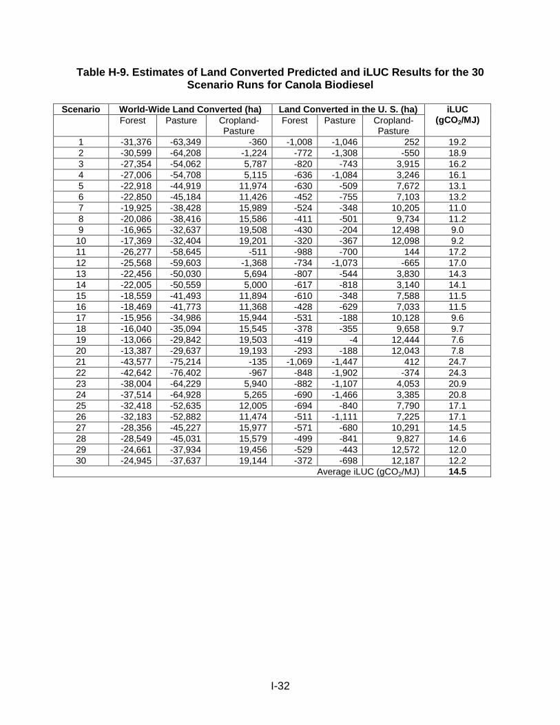
Land Use Change Effects for Canola Biodiesel The canola biodiesel land use change results presented in this section were produced using GTAP-BIO and the AEZ-EF models. Starting with the 2004 U.S. canola biodiesel production level of 0.0009 billion gallons, staff analysis used 400 million gallons of canola biodiesel shock for a total of 0.4009 billion gallons of U.S. canola biodiesel. Table H-9 provides details of land cover changes for each of the 30 scenario runs used in estimating iLUC values for canola biodiesel. It provides detailed land conversion for forest, pasture, and cropland pasture for all the 30 scenarios. Worldwide forest converted ranges from 0.01 to 0.04 Mha, pasture converted ranges from 0.03 to 0.08 Mha, and cropland pasture converted ranges from 0.00 to 0.02 Mha. For the United States, forest converted is small (< 0.001 Mha), pasture converted is also small (< 0.001 Mha), and cropland pasture converted ranges from 0.00 to 0.01 Mha. The Table also includes iLUC values for each of the 30 scenario runs used in the analysis and the average of all the runs. Figure H-9 shows a graphical plot of the land conversions detailed in Table H-9.
-450,000
-400,000
-350,000
-300,000
-250,000
-200,000
-150,000
-100,000
-50,000
0Forest Pasture Crop-Past
Hec
tare
s
Soy
U.S.
World
I-31
Table H-9. Estimates of Land Converted Predicted and iLUC Results for the 30 Scenario Runs for Canola Biodiesel
Scenario World-Wide Land Converted (ha) Land Converted in the U. S. (ha) iLUC
Figure H-9. Land Conversions Predicted by the Model for Canola Biodiesel
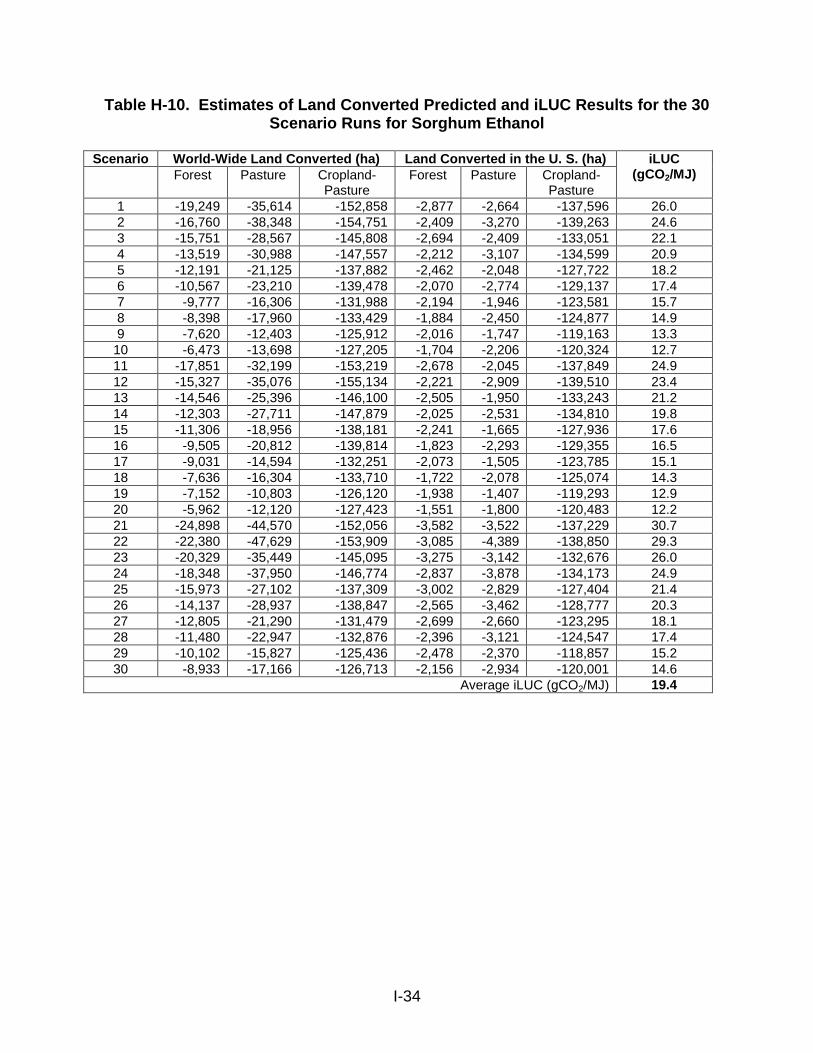
Land Use Change Effects for Sorghum Ethanol The sorghum ethanol land use change results presented in this section were produced using GTAP-BIO and the AEZ-EF models. Starting with the 2004 U.S. sorghum ethanol production level of 0.0005 billion gallons, staff analysis used an additional 400 million gallons of sorghum ethanol shock for a total shock of 0.4005 billion gallons of U.S. sorghum ethanol. Table H-10 provides details of land cover changes for each of the 30 scenario runs used in estimating iLUC values for sorghum ethanol. It provides detailed land conversion for forest, pasture, and cropland pasture for all the 30 scenarios. Worldwide forest converted ranges from 0.002 to 0.004 Mha, pasture converted ranges from 0.001 to 0.004 Mha, and cropland pasture converted ranges from 0.12 to 0.14 Mha. For the United States, forest converted ranges from 0.000 to 0.002 Mha, pasture converted ranges from 0.01 to 0.05 Mha, and cropland pasture converted ranges from 0.13 to 0.15 Mha. The Table also includes iLUC values for each of the 30 scenario runs used in the analysis and the average of all the runs. Figure H-10 shows a graphical plot of the land conversions detailed in Table H-10.
-100,000
-80,000
-60,000
-40,000
-20,000
0
20,000
40,000
Forest Pasture Crop-Past
Hec
tare
s Canola
U.S.
World
I-33
Table H-10. Estimates of Land Converted Predicted and iLUC Results for the 30 Scenario Runs for Sorghum Ethanol
Scenario World-Wide Land Converted (ha) Land Converted in the U. S. (ha) iLUC
Figure H-10. Land Conversions Predicted by the Model for Sorghum Ethanol
Land Use Change Effects for Palm Biodiesel The palm biodiesel land use change results presented in this section were produced using GTAP-BIO and the AEZ-EF models. Starting with the 2004 U.S. palm biodiesel production level of 0.00005 billion gallons, staff analysis used an additional 400 million gallons of palm biodiesel shock for a total shock of 0.40005 billion gallons of U.S. palm biodiesel. Table H-11 provides details of land cover changes for each of the 30 scenario runs used in estimating iLUC values for palm biodiesel. It provides detailed land conversion for forest, pasture, and cropland pasture for all the 30 scenarios. Worldwide forest converted ranges from 0.01 to 0.04 Mha, pasture converted ranges from 0.03 to 0.08 Mha, and cropland pasture converted ranges from 0.00 to 0.02 Mha. For Malaysia_Indonesia, forest converted ranges from 0.03 to 0.05 Mha, pasture converted is negligible (<0.00 Mha), and there is no cropland pasture change. The Table also includes iLUC values for each of the 30 scenario runs used in the analysis and the average of all the runs. Figure H-11 shows a graphical plot of the land conversions detailed in Table H-11.
-180,000
-160,000
-140,000
-120,000
-100,000
-80,000
-60,000
-40,000
-20,000
0Forest Pasture Crop-Past
Hec
tare
s Sorghum
U.S.
World
I-35
Table H-11. Estimates of Land Converted Predicted and iLUC Results for the 30 Scenario Runs for Palm Biodiesel
Scenari
o World-Wide Land Converted (ha) Land Converted in
Figure H-11. Land Conversions Predicted by the Model for Palm Biodiesel (Thousand ha)
7. Results from the Uncertainty Evaluations using Monte Carlo Simulations (MCS) The uncertainty analysis was performed using Monte Carlo analysis. As described earlier, the runs for the Monte Carlo analysis were conducted at the National Energy Research Scientific Computing center’s massively parallel computer cluster. Parameters from both the GTAP-BIO and AEZ-EF models were used for the uncertainty analysis. This is in contrast to the scenario analysis which used limited variations in the values of three of the most important parameters in the GTAP-BIO model to estimate iLUC emissions for each biofuel. Figures H-12 through H-17 provide probability distribution plots from the uncertainty analysis for each of the 6 biofuels. Details of distributions and ranges used for all of the parameters is provided in Attachment 4. Table H-12 provides a comparison of the averages from the scenario runs with the mean values from the uncertainty analysis. Even with limited variations in the values of the three parameters for the scenario runs, the average of the 30 runs for each biofuel is not significantly different from the mean iLUC values from the Monte Carlo runs (with hundreds of simulations).
-80,000
-70,000
-60,000
-50,000
-40,000
-30,000
-20,000
-10,000
0
10,000
Forest Pasture Crop-Past
Hec
tare
s Palm
Malaysia/Indonesia
World
I-37
Table H-12. Comparison of iLUC Values from Scenario runs and MCS
Figure H-12. Probability Distribution for Corn Ethanol
I-38
Figure H-13. Probability Distribution for Sugarcane Ethanol
I-39
Figure H-14. Probability Distribution for Soy Biodiesel
I-40
Figure H-15. Probability Distribution for Canola Biodiesel
I-41
Figure H-16. Probability Distribution for Sorghum Ethanol
I-42
Figure H-17. Probability Distribution for Palm Biodiesel
I-43
Attachment 1
Yield Price Elasticity (YPE) in the GTAP-BIO model
YPE is a parameter that has received the most feedback from stakeholders, particularly those from biofuel industries. This is because this parameter has special significance in the GTAP-BIO analysis: it has the largest influence on outputs from the model. This Attachment provides a review of studies and values for YPE reported by various authors. It also details the approach used by staff to consider using a range of values for this parameter in the current indirect land use change (iLUC) analysis. Yield Price Elasticity (YPE) is a parameter in the GTAP-BIO model which determines how much crop yield will increase in response to a price increase for the crop. It measures sensitivity of yield with respect to a crop price change assuming all other things constant. For example, if price yield elasticity is 0.25, a 10 percent increase in the price of the crop relative to input cost will result in a 2.5 percentage increase in crop yield. Review of Studies Houck and Gallagher41 pioneered work on YPE. They used data for corn in the United States for the time period 1951-1971. They employed different methodologies to analyze the data and reported values for YPE that ranged between 0.24 – 0.76. Menz and Pardey42 used the same data as Houck and Gallagher but came up with a value of 0.61 for data from 1951-1971 but reported values close to zero (and even negative) when using data from 1972-1980. Table 1-1 provides a summary of these studies and includes three additional studies with their respective reported values for price yield elasticity. Kenney and Hertel43 used a few select studies from Table 1-1 in their analysis and reported an average YPE value of 0.25 which has been widely cited by renewable fuel producers as the optimal value for this parameter. To be noted is that in Table 1-1, the reported elasticities range from 0.0 to 0.76. Keeney and Hertel, however, excluded the largest values in Table 1-1 (0.76; 0.69; and 0.61) from consideration on the grounds that the remaining “estimates rest on their relative modernity.” They also excluded ‘zero’ values and instead used the four remaining estimates (i.e., 0.24, 0.28, 0.27 and 0.22) to calculate a simple average value of 0.25 for yield price elasticity.
41 Houck, J.P., and P.W. Gallagher, “The Price Responsiveness of U.S. Corn Yields,” American Journal of Agricultural Economics 58 (1976): 731-734. 42 Menz, K.M., and P. Pardey, “Technology and U.S. Corn Yields: Plateaus and Price Responsiveness”. American Journal of Agricultural Economics 65 (1983): 558-562. 43 Keeney, R. and T. W. Hertel, “The Indirect Land Use Impacts of United States Biofuel Policies: The Importance of Acreage, Yield, and Bilateral Trade Responses”, American Journal of Agricultural Economics 91(4) (November 2009): 895–909.
Attachment 1-1
Berry44 in a report to the Air Resources Board as part of the Expert Working Group (EWG) proceedings, reviewed literature and data from the same studies shown in Table 1-1. Berry concluded that the Houck and Gallagher41 estimates should be excluded from the average because they are based on data from a time period 1951 through1971 and do not reflect more recent data for yield changes. Berry questioned the value of 0.27 for YPE in Choi and Helmberger45 on the ground that this estimate was inclusive of technological change, while the authors themselves stated that “yields are found to be quite insensitive to price." When Choi and Helmberger controlled for technological improvement via a time-trend, the yield-price correlation was negative. Berry, after reviewing these studies concluded that YPE was mostly zero and the largest value that could be used was 0.1.
Table 1-1 Literature Estimates of Corn Yield Elasticities
Authors Period Data, Method Elasticity Economy Houck & Gallagher41 1951-1971 TS* with log trends 0.76 United States Houck & Gallagher41 1951-1971 TS with log trends &
AC** 0.69 United States Houck & Gallagher41 1951-1971 TS with linear trends 0.28 United States Houck & Gallagher41 1951-1971 TS with linear trends &
AC 0.24 United States
Menz & Pardey42 1951-1971 TS with log trends & AC 0.61 United States
Menz & Pardey42 1972-1980 same as41 0$ & Neg. United States Choi & Helmberger45 1964-1988 TS without trend 0.27 United States Choi & Helmberber45 1964-1988 TS, OLS+ 0.0-0.27 United States Kaufman & Schnell46 1969-1987 TS, OLS 0.02 United States Lyons & Thompson47 1961-1973 Pooled time series 0.22 14 countries * TS = Time Series, ** AC = Acreage Control, $ Insignificant, + Ordinary least squares Since the Berry report was published, there have been additional studies related to YPE. These studies have also reported vastly different estimates of YPE. Roberts and Schlenker48 proposed that all of the relevant observed outcomes (output, yield, land, and price) are simultaneously determined in market equilibrium. They argued that ignoring the instrumental variables (or IV) methods and making use of simple correlation or Ordinary Least Squares (OLS) techniques would lead to incorrect and misleading
44 Berry, S.T., "Biofuels Policy and the Empirical Inputs to GTAP Models," Report to California Air Resources Board, evaluating GTAP (2011). http://www.arb.ca.gov/fuels/lcfs/workgroups/ewg/010511-berry-rpt.pdf 45 Choi J. S. and P. Helmberger, “How Sensitive are Crop Yields to Price Changes and Farm Programs?” Journal of Agriculture and Applied Economics 25 (1993):237-244. 46 Kaufman, R.K., and S.E. Snell, “A Biophysical Model of Corn Yield: Integrating Climatic and Social Determinants,” American Journal of Agricultural Economics, 79 (1997): 178-190. 47 Lyons, D.C., and R.L. Thompson, “The Effect of Distortions in Relative Prices on Corn Productivity and Exports: A Cross-Country Study,” Journal of Rural Development 4 (1981):83–102. 48 Roberts M.J. and W. Schlenker, "Identifying Supply and Demand Elasticities of Agricultural Commodities: Implications for the US Ethanol Mandate." National Bureau of Economic Research Working Paper (2010)15921.
Attachment 1-2
estimates49. They tested whether yields were themselves serially correlated and their analysis rejected this hypothesis. They concluded that yields were driven by weather and not by price. In a more recent analysis, Berry and Schlenker50 used U.S. state-level panel data51 and applied instrumental variables (IV) technique to estimate YPE. They reported that it was mainly the crop area (extensive margin) that responded to changes in prices caused by yield shocks and not the yield itself (intensive margin). They reported that the net YPE is not significantly different from zero (no higher than about 0.06 while area price elasticity is 0.25-0.30). The increased yield on existing land could be offset by the lower yield on “new land.” Considering the GTAP-BIO land cover structure, if the ratio of the productivity of marginal land to the existing land is 0.66,52 they concluded that the yield price elasticity for non-marginal land implies a YPE for non-marginal land that is no higher than 0.1. Huang and Khanna53 used U.S. county-specific, historical data for the period 1977-200754 to estimate yield responses of corn, soybeans and wheat to output prices and to changes in climate and technology over time. They also used instrumental variables (IV) regression methods to control for endogeneity of prices and county-specific fixed effects to control for unobserved location-specific effects on yield. They reported YPE values of 0.06 for soybeans, 0.15 for corn and 0.43 for wheat. Smith and Sumner55 used county level data between1961-2005 for the United States and applied ordinary least squares method and reported negative values for yield-price elasticities. They concluded that when corn prices increased, the use of fertilizer and pesticides also increased leading to higher yields but apparently not enough because of the loss of land productivity due to less crop rotation. Goodwin et al.56 used district level data for three states (Iowa, Indiana, and Illinois) in the United States for the period 1996-2010 for corn and soybeans. The authors applied
49 In Ordinary Least Square (OLS) estimation technique it is assumed the explanatory or independent variables (i.e. corn price) are independent from the variable to be explained (i.e. yield). That is, the line of causality goes say from price to yield. But when the two set of variables (the dependent and the “independent” ones) influence each other at the same time (have simultaneity) then the application of OLS is invalid for casual inference. Instead, instrumental variable methods allow consistent estimates when simultaneity is present. 50 Berry, S. and W. Schlenker, “Technical Report for the ICCT: Empirical Evidence on Crop Yield Elasticities,”: (2010) <http://www.arb.ca.gov/fuels/lcfs/09142011_iluc_sbreport.pdf> 51 They use U.S. data from the 30 states across the time period 1961-2009. They also use times series data for World/Regional (Brazil, China and Argentina and Thailand) to estimate YPE for corn, soybean and rise. They find little evidence of large positive yield-price elasticities with the exception of Brazil. 52 The ratio of marginal and average productivities measures the productivity of new cropland versus the productivity of existing cropland. In GTAP-BIO, the parameter for this ratio is called ETA. In earlier versions of the model, ETA = 0.66 in all regions and agro-ecological zones. 53 Huang, H. and M. Khanna, “An Econometric Analysis of U.S. Crop Yield and Cropland Acreage: Implications for the Impact of Climate Change.” Agricultural and Applied Economics Association Annual Meetings, Denver, Colorado (2010). 54 Their county level panel dataset includes 3015 continental U.S. counties over 31 time years. 55 Smith, A. and D. Sumner, “Estimating the Crop Yield Response to Price: Implications for the Environmental Impact of Biofuel Production,” (2011) University of California Davis. Work in Progress. 56 Goodwin B., M. Marra, N. Piggott and S. Mueller, “Is Yield Endogenous to Price? An Empirical Evaluation of Inter-and Intra-Seasonal Corn Yield Response,” (2012).
the ordinary least squares method and reported YPE of up to 0.008 for the intra-seasonal price movements and up to 0.25 for the inter-seasonal price changes.57 The intra-seasonal price movements were interpreted as the short-term elasticity and the inter-seasonal price changes as long-term elasticity. Using a regression analysis, the coefficient of this variable was used to compute intra-seasonal YPE and that of price of corn (or soybean) for inter-seasonal YPE. Pérez58 used Iowa farm level data from 1960-2004 and applied duality production theory and Bayesian estimation methods and reported a yield price elasticity of 0.29 for corn and 0.61 for soybeans. Table 1-2 summarizes the various current studies considered for ARB’s evaluation.
Table 1-2. Updated Literature Estimates of YPEs
Authors Period Elasticity Crop Data, Method
Huang & Khanna
1977-2007 0.15
U. S. Corn, soybean, and wheat
County level data, IV≠
Smith & Sumner 1961-2005
Neg. & Sig* U. S. Corn County level data, OLSº
Berry & Schlenker
1961-2009 0.1, 0 Net± U. S. Corn Country-level data, IV
Goodwin, et al. 1996-2010
0.01 SR 0.19-0.27 LR€
I States Corn “I-States” data, OLS
Pérez 1960-2004 0.29 Iowa Corn and soybeans
Iowa data, Duality-Bayesian
º OLS refers to Ordinary Least Squares * Immediate YPE is equal to -0.26 to 0.48; tow-year YPE is equal to -0.14 to 0.42 ± Net YPE is not significantly different from zero (no higher than about 0.06). € 0.006-0.0108 for “intra-seasonal” responsiveness interpreted as short run and 0.19-0.27 for “inter seasonal” responsiveness interpreted as long run. “I-States” is comprised of Iowa, Indiana, and Illinois. ≠ Instrumental variable The Elasticity sub-group of the LCFS Expert Workgroup59 composed of Bruce Babcock, Angelo Gurgel and Mark Stowers recommended keeping the central value of the yield elasticity with respect to price at 0.25 if only one value was used for all crops and all countries. If this elasticity could be varied, then it should be increased for crops-country combinations that could be double-cropped and should be decreased for combinations that cannot. As for the rationale for this recommendation, the group argued that the overall conclusion from the literature review is that the short-run (one-year) response of United States yield to price is quite inelastic with an average value of somewhere between 0.05 and 0.2. Double cropping and adoption of higher-yielding management
57 There is a large variation in their estimate of YPE for the three states in the sample. For example YPE for Illinois is three times larger than that of Indiana (0.15 vs. 0.45). 58 Pérez, J. F. R., “Essays on the environmental effects of agricultural production,” (Ph.D. dissertation, Iowa state University 2012). 59 ARB LCFS Expert Workgroup Final Recommendations from the Elasticity Values Subgroup,” (2010), http://www.arb.ca.gov/fuels/lcfs/workgroups/ewg/010511-final-rpt-elasticity.pdf
techniques were not considered in the Roberts and Schlenker48 study and hence the lower-bound in the medium to long run could not be zero and the GTAP-BIO should use elasticities that reflect a medium to long-term period instead of short run. One-year estimates common in the literature underestimated the long-run response of yields to price, and that farmers have an incentive to adopt higher-yielding seed technologies and other management techniques with higher prices but this could take five to 15 years. Based on these arguments, the elasticity sub-group recommended a reasonable increment to the short-run elasticity to account for long-run response was 0.05, which would bring the average value between 0.1 and 0.25. The group also recommended that if the GTAP-BIO model could assign different elasticities to different crops in different countries, then setting YPE to 0.175 for countries with no double cropping, 0.25 for the United States, and 0.3 for Brazil and Argentina would provide a more reasonable approximation to reality. Staff contracted with David Rocke from the University of California, Davis to perform a statistical analysis of the data used by some of the researchers in Table 1-2. David60 reviewed analysis (and data where available) for Goodwin et al.,56 Perez58, and Berry and Schlenker50 and additional studies and concluded that based on methodologically sound analyses, yield price elasticities are generally small to zero. Summary The assignment of a value for YPE for use in the GTAP-BIO model poses important challenges:
• Large majority of data for price and yields are for corn grown in the United States. There are no data for corn production outside the United States. Furthermore, most of the analysis has been for data from the Mid-Western region of the United States.
• Researchers use different econometric methods to derive relationship between yield and price. They sometimes report contrasting values even when using the same data.
• Most of the data used in published studies used data for crop yields and prices for periods that do not represent the current timeframe for biofuel production for the LCFS (2004-2012).
• Besides corn, GTAP-BIO includes paddy rice, wheat, canola, soybeans, palm, sorghum, etc. As currently used, any input value of YPE is used for all crops and regions in the model. Using YPE derived from corn for all crops (and regions) may bias the results one way or the other. The most optimal approach is to use crop and region specific YPEs derived from appropriate econometric treatment of data. However, there are currently no data available to estimate YPE by crop and by region. Hence it is not possible to use regional and crop-specific YPE in the GTAP-BIO model at the present time.
60 David Rocke, “Statistical Issues Related to the Low Carbon Fuel Standard”, Report submitted to the California Air Resources Board under Contract 13-405 (2014)
Attachment 1-5
• The model uses the same value of YPE for irrigated vs. rain-fed crops. It is likely that there are different responses to price changes between these two types of agricultural practices in different regions of the world.
• There is limited data for double-cropping for crops for all regions of the world. As suggested by stakeholders, double-cropping can be accounted by using a higher input value of YPE. However, in the current version of the GTAP-BIO model, net increase in crop yields includes effects related to price changes, crop switching, and extensification. Any change in the value of YPE must be calibrated to ensure that only double cropping effects are accounted by any increases in the value of YPE.
Taking all these into consideration and with a wide range of likely values for YPE from published literature, staff used a range of values between 0.05 and 0.35 to conduct scenario runs for all biofuels studied for the LCFS. These input values are used for all crops and regions for the 30 scenario runs conducted for each of the 6 biofuels.
Attachment 1-6
Attachment 2
Agro-ecological Zone Emission Factor (AEZ-EF) Model (v52)
This Page Left Intentionally Blank
Attachment 2-1
Agro-ecological Zone Emission Factor (AEZ-EF) Model (v52)
A model of greenhouse gas emissions from land-use change for use with AEZ-based economic models
Richard J. Plevin1, Holly K. Gibbs2, James Duffy3, Sahoko Yui1, Sonia Yeh1 1University of California—Davis, 2University of Wisconsin—Madison, 3California Air Resources Board
8 Model implementation ...................................................................................... 37
9 Summary of changes from v47 to v52 ............................................................ 42
10 References .............................................................. Error! Bookmark not defined.
Tables Table 1. Regions used in the GTAP-BIO and AEZ-EF models. (See also Figure 1.) ...... 4 Table 2. Estimates of deadwood by region or latitude (Mg C ha-1). ............................... 10 Table 3. IPCC default values for litter in mature forests (Mg C ha-1). ............................ 11 Table 4. Litter values used for forests in AEZ-EF model, by AEZ (Mg C ha-1). ............. 11 Table 5. Understory carbon values used in AEZ-EF (Mg C ha-1). ................................. 13 Table 6. Weighted fraction of AGLB carbon remaining after 30 years........................... 14 Table 7. IPCC grassland biomass data (Mg dry biomass ha-1). .................................... 14 Table 8. Grassland biomass data used in AEZ-EF. ...................................................... 14 Table 9. Parameters used to compute total biomass carbon from crop yield. ............... 15 Table 10. Other parameters used to compute total biomass carbon from crop yield for crops. ............................................................................................................................ 17 Table 11. Transition sequences modeled ...................................................................... 20 Table 12. Order of allocation of land to transition sequences ........................................ 20 Table 13. Fraction of forest change attributable to deforestation, by GTAP-BIO region. ...................................................................................................................................... 21 Table 14. Summary of carbon stock changes counted for each land cover transition. .. 23 Table 15. Fraction of forest clearing by fire in each GTAP-BIO region. ......................... 27 Table 16. Global warming potentials used in AEZ-EF. .................................................. 28 Table 17. Forest burning emission factors (kg Mg-1 dry matter). ................................... 29 Table 18. Pasture burning emission factors (kg Mg-1 dry matter). ................................. 29 Table 19. Fraction of forest clearing by fire in each GTAP-BIO region. ......................... 29 Table 20. Foregone sequestration rates (Mg C ha-1 y-1). ............................................... 30 Table 21. Soil carbon stock change factors used in AEZ-EF. ....................................... 32 Table 22. Mapping of stock change factors to AEZs in AEZ-EF. ................................... 32 Table 23. Starting row for land cover change matrices, and the coefficient in the generated landcover.har file that holds the corresponding data. ................................... 40
Figures
Figure 1. Distribution of agro-ecological zones (AEZs 1-18) and regions used in the GTAP-BIO model. Shades of red, green, and blue represent tropical, temperate, and boreal AEZs, respectively. ............................................................................................... 6 Figure 2. Fraction of AGLB remaining in HWP after 30 years. ...................................... 13 Figure 3. Example figure from "Results" worksheet, showing emissions by transition sequence for a trial run for soybean biodiesel. .............................................................. 19 Figure 4. Example of landchange.har, which is generated by LUC.exe ........................ 42
Attachment 2-2
1 Overview
The purpose of the agro-ecological zone emission factor model (AEZ-EF) is to estimate the total CO2-equivalent emissions from land use changes, e.g., from an analysis of biofuels impacts or policy analyses such as estimating the effect of changes in agricultural productivity on emissions from land use. The model combines matrices of carbon fluxes (Mg CO2 ha-1 y-1) with matrices of changes in land use (ha) according to land-use category as projected by GTAP or similar AEZ-oriented models. As published, AEZ-EF aggregates the carbon flows to the same 19 regions (Table 1) and 18 AEZs (Figure 1) used by GTAP-BIO, the version of GTAP currently used by Purdue University researchers for modeling CO2 emissions from indirect land-use change (ILUC) (e.g., Tyner, Taheripour et al. 2010)61. The model, however, is designed to work with an arbitrary number of regions, as described in section 8.4. The AEZ-EF model contains separate carbon stock estimates (Mg C ha-1) for biomass and soil carbon, indexed by GTAP AEZ and region, or “Region-AEZ” (Gibbs and Yui 201162; Gibbs, Yui et al. 201463). The model combines these carbon stock data with assumptions about carbon loss from soils and biomass, mode of conversion (i.e., whether by fire), quantity and species of carbonaceous and other greenhouse gas (GHG) emissions resulting from conversion, carbon remaining in harvested wood products and char, and foregone sequestration.64 The model relies heavily on IPCC greenhouse gas inventory methods and default values (IPCC 2006)10, augmented with more detailed and recent data where available.
The AEZ-EF model was designed for use with a static comparative economic model, i.e., one that starts with a baseline and computes a new equilibrium in one step, rather than as a series of steps over time. Handling a dynamic analysis properly would require tracking the carbon status of land that may be going through a series of conversions and reversions. This could be done if the carbon accounting were performed in the GTAP TABLO code, but this is clearly beyond the scope of the current model and report. A very simple approach to using the AEZ-EF model with a dynamic economic analysis would be to compute the change in land-cover areas by AEZ and region between the starting and ending states and to apply the emission factor model to these changes in the same way it is used for the static model.
1.1 Sinks and sources of greenhouse gas emissions from land use change
Following the IPCC GHG inventory guidelines, the AEZ-EF model includes the following sources / sinks of greenhouse gas emissions:
1. Above-ground live biomass (trunks, branches, foliage)
61 Tyner, W. E., F. Taheripour, Q. Zhuang, D. K. Birur and U. Baldos, “Land Use Changes and Consequent CO2 Emissions due to US Corn Ethanol Production: A Comprehensive Analysis.” West Lafayette, IN, Dept. of Agricultural Economics, Purdue University (2010): 90. http://www.transportation.anl.gov/pdfs/MC/625.PDF. 62 Gibbs, H. K. and S. Yui, (2011) “New Spatially-Explicit Estimates of Soil and Biomass Carbon Stocks by GTAP Region and AEZ,” U. Wisconsin-Madison and University of California-Davis 63 Gibbs, H., S. Yui and R. J. Plevin, “New Estimates of Soil and Biomass Carbon Stocks for Global Economic Models. Global Trade Analysis Project (GTAP) Technical Paper” No. 33 (2014). GTAP Technical Papers. West Lafayette, Indiana, Center for Global Trade Analysis, Department of Agricultural Economics, Purdue University. https://www.gtap.agecon.purdue.edu/resources/res_display.asp?RecordID=4344. 64 A version of this model implemented in the Python language includes estimates of uncertainty in all parameters, thereby enabling quantitative analysis of uncertainty in the AEZ-EF model separately or in conjunction with the GTAP-BIO model.
2. Below-ground live biomass (coarse and fine roots) 3. Dead organic matter (dead wood and litter) 4. Soil organic matter 5. Harvested wood products 6. Non-CO2 climate-active emissions (e.g., CH4 and N2O) 7. Foregone sequestration
In this report, we use the following definitions and acronyms: • Above-ground live biomass (AGLB): trunk, branches, and foliage • Dead organic matter (DOM): standing and downed dead trees, coarse woody debris, and
litter • Above-ground biomass (AGB): AGLB plus DOM • Total AGLB: AGLB + understory • Total AGB: AGB + understory • Below-ground biomass (BGB): coarse and fine roots • Soil organic carbon (SOC) • Total ecosystem biomass (TEB): Total AGB + BGB • Total ecosystem carbon (TEC): SOC + carbon fraction of TEB
Table 1. Regions used in the GTAP-BIO and AEZ-EF models. (See also Figure 1.)
Region ID Description USA United States EU27 European Union 27 Brazil Brazil Canada Canada Japan Japan ChiHkg China and Hong Kong India India C_C_Amer Central and Caribbean Americas S_O_Amer South and Other Americas E_Asia East Asia Mala_Indo Malaysia and Indonesia R_SE_Asia Rest of South East Asia R_S_Asia Rest of South Asia Russia Russia Oth_CEE_CIS East Europe and Rest of Former Soviet Union Oth_Europe Rest of European Countries ME_N_Afr Middle Eastern and North Africa S_S_Afr Sub Saharan Africa Oceania Oceania (Source: Tyner, Taheripour et al. 2010)1
Attachment 2-4
1.2 Data sources
The AEZ-EF model includes global data that describe carbon stocks in above- and below-ground live biomass and in soils beneath forests and pastures. Forest AGLB is derived from various remote-sensing and ground-based sources, whereas pasture AGLB is gathered from the literature. Soil carbon data are from the Harmonized World Soil Database (HWSD)65, from which we produced SOC estimates to depths of 30 cm and 100 cm aggregated for each Region-AEZ (Gibbs, Yui et al. 2014)2. Below-ground biomass carbon for all land cover types is based primarily on root:shoot ratios (Saatchi, Harris et al. 2011)66, except for the pan-tropics. Peatland, deadwood, and litter carbon stocks are taken from the literature. (Specific sources are described below.) The AEZ-EF model combines these carbon stock data with assumptions about carbon dynamics that together determine the CO2-equivalent emissions associated with land-use conversion. These assumptions, described later in this report, include:
• The fraction of soil carbon lost or gained upon conversion • Sequestration rates (Mg C ha-1 y-1) for forests (foregone if converted) • Growth rates (Mg C ha-1 y-1) for forests growing on onetime pasture or cropland • The fraction of conversion achieved using fire • The non-CO2 emissions associated with land clearing using fire • N2O emissions associated with the loss of soil organic carbon • The fraction of forest AGLB that is harvested and remains sequestered in wood products
at the end of the analytical horizon (currently 30 years).
2 Carbon stock aggregation
The C stock database contains area-weighted averages of above- and below-ground C stocks by land cover class, aggregated to Region-AEZ boundaries (Gibbs, Yui et al. 2014)2. The method of aggregation selected affects the emission factors that are generated. Computing area-weighted averages is clearly the simplest approach, and does not require additional data. However, this method provides a good proxy for land selection only if selection is random across each land cover class, or if there is little variance in C stock across each class. A more sophisticated approach (though the data are impoverished and not necessarily more accurate) would weight C stocks by likelihood of conversion, based on suitability, accessibility, evidence from remote sensing analysis, and so on. For example, a simple, first-order approach would be to use relative proximity to roadways as a proxy for likelihood of conversion.67
65 FAO/IIASSA/ISRIC/ISS-CAS/JRC (2009). Harmonized World Soil Database (version 1.1), FAO, Rome, Italy and IIASA, Laxenburg, Austria. http://www.iiasa.ac.at/Research/LUC/External-World-soil-database/HWSD_Documentation.pdf. 66 Saatchi, S. S., N. L. Harris, S. Brown, M. Lefsky, E. T. A. Mitchard, W. Salas, B. R. Zutta, W. Buermann, S. L. Lewis, S. Hagen, S. Petrova, L. White, M. Silman and A. Morel, "Benchmark map of forest carbon stocks in tropical regions across three continents." Proceedings of the National Academy of Sciences (2011). 67 A “road-proximity rule” will not be appropriate throughout the tropics. Depending on historical land use, roads may actually reduce the likelihood of clearing in regions with sparse forest cover. It may only be relevant for the heart of the Amazon and Congo basins and the Papua province of Indonesia. But roads and ports are planned in
Application of a likelihood-of-conversion criterion produces a preference order for land conversion and converts the C stock database from one of average values to one representing marginal values. Marginal values are generally scale-dependent, i.e., the marginal land source (and thus emissions) will vary as more land is utilized in a region. It would thus be useful to explore the variance in marginal emissions across relevant scales, not only of biofuel demand but of global land demand under different assumptions regarding food production (e.g., in light of crop losses from extreme weather events.)
2.1 Comparing carbon stocks with those in earlier ILUC modeling
We note that the prior emission factor model used by the California Air Resources Board (CARB) relied on data from the Woods Hole Research Center (WHRC) and aggregated emission factors to slightly different GTAP regional boundaries, based on an estimate of the percentage of land conversion in each region that involved particular ecosystem types. For example, if the newly cropped land in a given region was previously 40% forest and 60% grassland, it was assumed that any addition of cropland projected by GTAP-BIO to occur in that region would be converted 40% from forest and 60% from grassland. Thus, although the regional carbon stock estimates from the AEZ-EF model can be compared with those of the former model, the use of area weighting in the AEZ-EF and historical conversion weightings in the earlier model means these two approaches—by definition—estimate different quantities. However, the final emission factors are commensurable as both models estimate the emissions associated with biofuel-induced LUC, albeit using different methods and data.
Figure 1. Distribution of agro-ecological zones (AEZs 1-18) and regions used in the GTAP-BIO model. Shades of red, green, and blue represent tropical, temperate, and boreal AEZs, respectively.
2.2 Mapping to GTAP-BIO boundaries and economic uses
GTAP-BIO considers land to be in one of five usage categories: 1. Forestry (accessible, by definition)
these regions so conditions will be dynamic over the next 5-10 years. Thus we could consider making some rough assumptions to see if there is an impact on the results, but this would not necessarily be an improvement.
Attachment 2-6
2. Livestock pasture 3. Cropland (including the subset cropland-pasture) 4. Unmanaged (non-forest, not in current economic use) 5. Inaccessible (because of a lack of infrastructure or other restrictions)
However, GTAP-BIO considers land competition and conversion only among forestry, pasture and cropland; it excludes land deemed unmanaged and inaccessible (Golub and Hertel 2012)68. Excluding inaccessible forest from the analysis tends to underestimate the conversion of forest as a result of price changes (Gouel and Hertel 2006)69. The carbon data used in AEZ-EF have been aggregated to GTAP-BIO boundaries, but they include both accessible and inaccessible forests, as well as grasslands other than those used for livestock grazing, and thus represent broader resources than those represented in GTAP-BIO. Some of the issues involved in these differing representations are discussed below.
3 Biomass carbon stocks
3.1 Forestry
Ideally, the carbon stocks for each Region-AEZ would represent the same land represented by GTAP-BIO, that is, only accessible forests rather than all forests in a given AEZ. However, the data that quantify accessible versus inaccessible forest are not spatially explicit, but are based on FAO national data and percentages in each category (Gibbs, Yui et al. 2014)2. We followed the approach taken by WHRC and Winrock to produce average C stocks that combine accessible and inaccessible forests. We also mask out land identified by the GTAP maps as “unmanaged,” since this includes shrublands and grasslands not used for grazing. Forest areas are not based on the GTAP definition because the GTAP forest map does not account for areas cleared by logging or for other non-agricultural purposes (Gibbs, Yui et al. 2014)2. Thus, we use the GTAP-BIO cropland and pasture boundaries but rely on satellite data for forest boundaries.
3.1.1 Below-ground biomass
Below-ground biomass stocks are generally estimated using root:shoot ratios, which vary by species and region. In CARB’s previous model of ILUC emissions, BGB was included in estimates of biomass carbon from the Woods Hole Research Center (WHRC). The new carbon stock data (Gibbs, Yui et al. 2014)2 break out above- and below-ground data based largely on IPCC (2006)70 recommendations. AEZ-EF model explicitly includes estimates of below-ground biomass and the gain or loss thereof for conversions of among forest, pasture, and cropland. It was not possible to have separate belowground and aboveground biomass layers specific
68 Golub, A. A. and T. W. Hertel, "Modeling land-use change impacts of biofuels in the GTAP-BIO framework." Climate Change Economics 03(03) (2012): 1250015. 69 Gouel, C. and T. Hertel (2006). Introducing Forest Access Cost Functions into a General Equilibrium Model. GTAP Research Memoranda, Purdue University. https://www.gtap.agecon.purdue.edu/resources/download/2899.pdf. 70 IPCC (2006). "2006 IPCC Guidelines for National Greenhouse Gas Inventories, Volume 4: Agriculture, Forestry and Other Land Use."
for each dataset because not all databases provide this information separately. The following methods were used to create separate above- and below-ground biomass values:
• For data from Saatchi, Harris et al. (2011)6, we created a look-up table based on the allometric equation described below to estimate root-to-shoot ratios71.
• For boreal forests and tropical forests with data from sources other than Saatchi et al. (2011)6, we used root-to-shoot ratios based on total tree biomass from the widely used IPCC GPG (IPCC 2006)72, as shown in Table 4. Note that AEZs 1-6 indicate tropical regions, and AEZs 13-18 indicate boreal regions. In some cases, the values were averaged as the translation between AEZs and the IPCC ecological zones were not exact.
• For temperate forests a root-to-shoot ratio of 0.25 was assumed in all cases.
Forest carbon data for Russia (sourced from WHRC) represent total biomass, including AGB, BGB, and understory carbon. We use a default root:shoot ratio of 0.25 to convert the total biomass to AGB and BGB, and for this region, we apply a value of 0 Mg ha-1 in the model for understory carbon to avoid double-counting. We recognize that this implicitly assigns a root:shoot ratio of 0.25 to understory biomass, but any error caused by the small difference in this small quantity in a single region is likely of little consequence.
3.1.2 Carbon stored in dead organic matter
Forest biomass carbon estimates (including our own database) include only live tree trunks, branches, and foliage. In addition to live biomass, forests also often contain a substantial quantity of dead organic matter (DOM). For example, according to the US Forest Inventory, 35% of the total forest carbon pool is in live vegetation, 52% in soil, and 14% in dead organic matter, excluding fine woody debris (Woodall, Heath et al. 2008)73. Elsewhere, these ratios vary across climatic zones.
DOM consists of litter and deadwood. Deadwood includes all non-living tree biomass not included in litter, including standing dead trees, down dead trees, dead roots, and stumps larger than a specific diameter, often 10 cm (Woodall, Heath et al. 2008)13. Although the IPCC implies that litter refers to the organic layers on the surface of mineral soils, soil science, by contrast, considers litter to be restricted to freshly fallen leaves, and regards decomposing leaves as humus (Takahashi, Ishizuka et al. 2010)74. The IPCC guidelines assume that dead organic matter stocks are zero for non-forest land-use categories. The Tier 1 IPCC GHG inventory guidelines assume that deadwood and litter carbon stocks are in equilibrium, i.e., that there are no net emissions
71 Root-to-shoot ratios relate the belowground biomass quantities to the aboveground biomass. They are routinely used because aboveground biomass in an easier quantity to measure through field plots or remote sensing imagery. The correlations between above and belowground biomass are established through detailed field analysis at a limited number of plots (harvesting, drying and weighing the entire plant to weight the biomass). 72 Using Table 4.4, references included Mokany et al 2006, Lie et al 2003, and Fittkau and Klinge 1997 73 Woodall, C. W., L. S. Heath and J. E. Smith, "National inventories of down and dead woody material forest carbon stocks in the United States: Challenges and opportunities." Forest Ecology and Management 256(3) (2008): 221-228. 74 Takahashi, M., S. Ishizuka, S. Ugawa, Y. Sakai, H. Sakai, K. Ono, S. Hashimoto, Y. Matsuura and K. Morisada, "Carbon stock in litter, deadwood and soil in Japan’s forest sector and its comparison with carbon stock in agricultural soils." Soil Science & Plant Nutrition 56(1) (2010): 19-30.
Attachment 2-8
from this pool. However, the inventory guidelines provide estimates for litter but not for deadwood. Assuming that deadwood and litter stocks are in equilibrium, conversion of forest to pasture or cropland releases the carbon in these pools and ends the processes that replenish these pools. Since the biomass stock rates and growth rates we use are net of mortality, the CO2 from combustion of dead wood and litter is a source of additional emissions.
3.1.2.1 Deadwood
The quantity of deadwood in a forest depends on several factors; these include the density of live trees, the age of the forest, temperature, humidity, harvest frequency, self-thinning mortality, time elapsed since the last disturbance, and whether this was fire, which removes dead wood, or an event that introduces deadwood, such as blow-downs, diseases, or pests. Because of these diverse influences, there is no predictive relationship between the stocks of live tree biomass carbon and deadwood carbon (Woodall and Westfall 2009)75. Ratio methods fail spectacularly in cases of low live and high dead biomass. Large-scale disturbances are location-specific, so it is difficult to generalize from these results. To complicate matters further, deadwood is infrequently measured. What empirical data do exist are based on diameter measurements, from which volume and carbon are estimated (Woodall, Heath et al. 2008)13. The carbon density of deadwood varies with the state of decay, adding further uncertainty to the magnitude of this carbon pool.
The amount of deadwood in forests is highly variable around the world, and range from 0 to >600 Mg biomass ha-1, but most forests contain 30 to 200 Mg biomass ha-1 of deadwood (Richardson, Peltzer et al. 2009)76. Estimates of coarse woody debris (CWD) – fallen dead trees and large branches – in tropical forests vary widely from 0 to >60 Mg biomass ha-1 (Baker, Honorio Coronado et al. 2007)77. The IPCC defines deadwood as “the carbon in coarse woody debris, dead coarse roots, standing dead trees, and other dead material not included in the litter or soil carbon pools” (IPCC 2006)10, so CWD is a subset of DOM.
In a study of deadwood in New Zealand’s forests, Richardson, Peltzer et al. (2009)16 found that at a plot scale, there was a weak positive relationship between total live tree biomass and deadwood, and a negative relationship between the percentage of above-ground biomass as deadwood and live tree biomass. However, they conclude:
At a small scale, in even-aged stands, there should be a negative relationship between live tree biomass and deadwood biomass reflecting the reciprocal oscillation of forest biomass between live and dead pools (Lambert et al., 1980; Allen et al., 1997). However, in this national-scale analysis, live tree and deadwood biomass were weakly positively correlated because plots containing large-sized tree species produced larger pieces of deadwood. This positive relationship between live tree and deadwood biomass was also retained within forest types because our broad forest types all contain a wide range of tree sizes and environments.
In the case of New Zealand, they conclude that the mass of deadwood is approximately 16% of the live tree biomass. For the scale of analysis in GTAP-BIO and the AEZ-EF model, it
75 Woodall, C. W. and J. A. Westfall, "Relationships between the stocking levels of live trees and dead tree attributes in forests of the United States." Forest Ecology and Management 258(11) (2008): 2602-2608. 76 Richardson, S. J., D. A. Peltzer, J. M. Hurst, R. B. Allen, P. J. Bellingham, F. E. Carswell, P. W. Clinton, A. D. Griffiths, S. K. Wiser and E. F. Wright, "Deadwood in New Zealand's indigenous forests." Forest Ecology and Management 258(11) (2008): 2456-2466. 77 Baker, T. R., E. N. Honorio Coronado, O. L. Phillips, J. Martin, G. M. van der Heijden, M. Garcia and J. Silva Espejo, "Low stocks of coarse woody debris in a southwest Amazonian forest." Oecologia 152(3) (2007): 495-504.
Attachment 2-9
is reasonable to estimate the size of the deadwood pool based on the pool of above-ground live biomass. In Japan, Takahashi, Ishizuka et al. (2010)14 found that deadwood carbon stocks for coniferous plantations with a history of non-commercial thinning showed 17.1 Mg C ha-1 and semi-natural broad-leaved forests showed 5.3 Mg C ha-1 on average, although these values are based on limited data. Oswalt, Brandeis et al. (2008)78 found that on the Caribbean island of St. John, deadwood materials contributed 8.9±0.8 (SE) Mg C ha-1, while litter contributed a mean of 5.8 ± 0.6 Mg C ha-1. Thus, despite the uncertainties, the amount of DOM in forests is clearly non-negative: excluding it (which is equivalent to assigning a value of zero) would bias C stock estimates. Most of this carbon would be released quickly upon conversion by fire. These C stocks were not accounted for in the original ARB ILUC model or in the EPA/Winrock model. Estimates of carbon stored in deadwood used in AEZ-EF are derived from Pan et al. (2011)79. The US, Europe, and Canada are shown separately in the Pan et al. data19, and since these correspond to regions used in the GTAP-BIO model, the values are adopted directly. For other areas, the average values from Pan et al19. for boreal, temperate, and tropical latitudes are used according to the latitude of the region, as shown in Table 2. Table 2. Estimates of deadwood by region or latitude (Mg C ha-1).
Region or latitude Deadwood USA 10.5 EU27 2.1 Canada 21.8 Boreal 14.3 Temperate 4.2 Tropical 27.5 Source: Pan, Birdsey et al.(2011)
3.1.2.2 Litter
The IPCC gives litter values for two categories of mature forests: broadleaf deciduous and needleleaf evergreen. However, their regional boundaries do not conform exactly to AEZs. To use these values, three methods must be developed:
1. A means to map the IPCC spatial aggregation to AEZs 2. A means to combine the broadleaf deciduous and needleleaf evergreen values into a
single value 3. A protocol to adjust the value for mature forests to reflect the forests actually converted
The AEZ-EF model simply averages the values for broadleaf deciduous and needleleaf evergreen forests, and averages the two values (cold and warm) for dry temperate forests and for moist
78 Oswalt, S. N., T. J. Brandeis and C. W. Woodall, "Contribution of Dead Wood to Biomass and Carbon Stocks in the Caribbean: St. John, U.S. Virgin Islands." Biotropica 40(1) (2008): 20-27. 79 Pan, Y., R. A. Birdsey, J. Fang, R. Houghton, P. E. Kauppi, W. A. Kurz, O. L. Phillips, A. Shvidenko, S. L. Lewis, J. G. Canadell, P. Ciais, R. B. Jackson, S. Pacala, A. D. McGuire, S. Piao, A. Rautiainen, S. Sitch and D. Hayes, "A Large and Persistent Carbon Sink in the World's Forests." Science 333 (2011): 988-993.
Attachment 2-10
temperate forests. Table 3 lists the IPCC’s default values for litter in mature forests. Table 4 lists the values used in AEZ-EF, by AEZ. Table 3. IPCC default values for litter in mature forests (Mg C ha-1).
Latitude/humidity Broadleaf deciduous Needleleaf evergreen Average
a Values in parentheses marked by superscript “a” are the 5th and 95th percentiles from simulations of inventory plots, while those without the superscript indicate the entire range. Table 4. Litter values used for forests in AEZ-EF model, by AEZ (Mg C ha-1).
The forest understory consists of shrubs, herbs, grasses, mosses, lichens, and vines. Carbon stocks in the understory increase as gaps appear in the canopy and decrease as the canopy closes, so these are inversely proportional to forest carbon stock to a degree (Plantinga and Birdsey 1993)80. Thus, for regrowing forests with low carbon densities, the exclusion of understory biomass would be expected to underestimate carbon stocks and thus emissions. Understory carbon is added separately in AEZ-EF except in the case of Russia, where the biomass stock estimates (from WHRC) already include this pool. Woodbury et al. (2007)81 examined carbon sequestration in the US forest sector, and suggested that the minimum understory carbon density is about 0.5% of the tree carbon density found in mature stands where density is high. Woodbury et al21. note: “The maximum understory carbon density is predicted to occur when the plot contains no trees greater than 2.54 cm in diameter, and ranges from 1.8 to 4.8 t C ha-1, depending on forest type.” These studies permit us to use the minimum of 0.5% of AGLB or a maximum of 4.8 Mg C ha-1, at least in US forests. Some studies note that understory biomass has a negative exponential relationship to tree biomass, since canopy openings increase understory growth and closed canopies reduce it. Thus any factor multiplied by AGLB is questionable. Telfer (1972)82 finds a grand total of 2.5 to 8.9 Mg biomass (or 1.2 to 4.5 Mg C) per ha in Nova Scotia, with mosses comprising a large component.
In their Amazonian rainforest studies, Nascimento et al. (2002)83 find an average of 1.28 Mg biomass ha-1 of stemless plants plus 8.30 Mg biomass ha-1 of lianas (woody vines that hang from trees), totaling 9.6 Mg biomass, or about 4.8 Mg C ha-1, in addition to the large and small trees. They conclude that biomass in herbs, epiphytes, and climbing vines are less abundant in the Amazonian rainforest than in many other neotropical forests, and suggest that a value of 4.5 to 5 Mg C ha-1 for understory carbon in tropical rainforests would be conservative. Cummings et al. (2002)84 find a mean biomass of live "non-tree" components in the Brazilian Amazon of equal to 22 Mg biomass or about 11 Mg C ha-1. This includes palms that they consider "non-tree" species. They calculate a total of 18.5 Mg biomass ha-1 of non-tree live biomass (seedlings + palms + vines) in open forest, 17.7 Mg biomass ha-1 in dense forest, and about 40 Mg biomass ha-1 in ecotone forest (edge forests in contact with savanna and any of the other classes of forest formations).
Table 5 shows the estimates of understory biomass used in AEZ-EF. For boreal forests and temperate forests, we use a value of 3 Mg C ha-1, a round value approximately in the middle of the ranges suggested by Telfer (1972)22 and Woodbury et al. (2007)21, respectively. For
80 Plantinga, A. J. and R. A. Birdsey, "Carbon fluxes resulting from U.S. private timberland management." Climatic Change 23(1) (1993): 37-53. 81 Woodbury, P. B., J. E. Smith and L. S. Heath, "Carbon sequestration in the U.S. forest sector from 1990 to 2010." Forest Ecology and Management 241(1-3) (2007): 14-27. 82 Telfer, E. S., "Understory biomass in five forest types in southwestern Nova Scotia." Canadian Journal of Botany 50(6) (1972): 1263-1267. 83 Nascimento, H. E. M. and W. F. Laurance, "Total aboveground biomass in central Amazonian rainforests: a landscape-scale study." Forest Ecology and Management 168(1-3) (2002): 311-321. 84 Cummings, D. L., J. Boone Kauffman, D. A. Perry and R. Flint Hughes, "Aboveground biomass and structure of rainforests in the southwestern Brazilian Amazon." Forest Ecology and Management 163(1-3) (2002): 293-307.
Attachment 2-12
tropical forests, we use the mean value (11 Mg C ha-1) found by Cummings et al. (2002)24 for the Brazilian Amazon. Table 5. Understory carbon values used in AEZ-EF (Mg C ha-1).
Latitude Mg C ha-1 Boreal 3.0 Temperate 3.0 Tropical 11.0
3.1.4 Carbon stored in harvested wood products (HWP)
Some harvested forest carbon remains sequestered in wood products for the full analytic time horizon used in AEZ-EF, 30 years. To estimate the carbon remaining after this period requires estimates of the volume of wood harvested, the fraction that is converted to long-lived products, and the fate of those products over time, as well as the fractions added to landfills and the fractions of the landfill biomass sequestered long term, emitted as CH4, or combusted for energy generation either as biomass or CH4. AEZ-EF uses values derived from a study by Earles, Yeh, and Skog (2012)85, listed in Table 6, based on the values shown in Figure 2.
Figure 2. Fraction of AGLB remaining in HWP after 30 years. Source: Earles, Yeh and Skog (2012)25
We note that the fraction of HWP that remains sequestered after 30 years is lower than the fraction originally harvested because some wood is lost in the production of wood products. The model currently uses a single parameter to represent both the reduction in fuel load and long-term sequestered carbon. However, since the wood that is removed but not sequestered is in many cases combusted, we feel that this is an acceptable approximation. We also note that Earles, Yeh, and Skog (2012)25 do not include landfill emissions of CO2 or CH4, nor (obviously) whether the CH4 is vented or captured for energy production.
85 Earles, J. M., S. Yeh and K. E. Skog, "Timing of carbon emissions from global forest clearance." Nature Clim. Change 2 (2012).
Attachment 2-13
3.2 Pasture
Pasture carbon stock values are based on IPCC 200610 GHG Inventory Guidelines, using Tier I defaults for grasslands. Table 7 lists IPCC grassland biomass data (IPCC 2006, Table 6.4)10; Table 8 shows how these values are mapped to AEZs in the AEZ-EF model. Table 6. Weighted fraction of AGLB carbon remaining after 30 years. (weighted by total above ground biomass in each country).
Region HWP fraction Region HWP fraction Brazil 7% Oceania 13% C_C_Amer 5% Oth_CEE_CIS 30% Canada 28% Oth_Europe 34% ChiHkg 6% R_S_Asia 3% E_Asia 6% R_SE_Asia 3% EU27 35% Russia 35% India 2% S_O_Amer 5% Japan 7% S_S_Afr 2% Mala_Indo 4% USA 36% ME_N_Afr 9% Table 7. IPCC grassland biomass data (Mg dry biomass ha-1).
Zone ID Latitude Humidity Peak AGLB root:shoot BGB Total 1 Boreal Dry & Wet 1.7 4.0 6.8 8.5 2 Temperate Cold, dry 1.7 2.8 4.76 6.46 3 Temperate Cold, wet 2.4 4. 0 9.6 12.0 4 Temperate Warm, dry 1.6 2.8 4.48 6.08 5 Temperate Warm, wet 2.7 4.0 10.8 13.5 6 Tropical Dry 2.3 2.8 6.44 8.74 7 Tropical Moist & wet 6.2 1.6 9.92 16.12 8 Temperate Dry (avg cold & warm) 1.65 2.8 4.62 6.27 9 Temperate Wet (avg cold & warm) 2.55 4.0 10.2 12.75 Source: IPCC 200610 GHG Inventory Guidelines, table 6.4. The IPCC indicates a nominal estimate of error of ±75% (two times the standard deviation, as a percentage of the mean) for the total biomass stocks.
To estimate the AGB on cropland after conversion from pasture, cropland pasture, or forest, or of cropland prior to reversion to these categories, prior versions of AEZ-EF used an estimate of annual net primary productivity (NPP) of C4 plants86, estimated using the Terrestrial Ecosystem Model (TEM) by AEZ and by region. These are the same data used in GTAP-BIO to estimate the relative productivity of newly converted cropland. In the current version of the model, the post-conversion yield for each crop is computed using GTAP-BIO’s endogenous projections of production and area harvested, dividing the former by the latter to produce yield by crop (sector), region, and AEZ (Mg biomass ha-1). This approach allows any uncertainties that propagate through GTAP-BIO to its projections of yield (e.g., in response to price changes) to be transmitted to the AEZ-EF model so the two models use identical yield assumption. In addition, yield is now crop- and location- specific. Table 9. Parameters used to compute total biomass carbon from crop yield.
86 From http://www.biology-online.org/dictionary/C4_plant: A C4 plant is one in which the CO2 is first fixed into a compound containing four carbon atoms before entering the Calvin cycle of photosynthesis. A C4 plant is better adapted than a C3 plant in an environment with high daytime temperatures, intense sunlight, drought, or nitrogen or CO2 limitation.
(Source: West, Brandt, et al. 2010, adjusted as per email exchange with T. West.)87 To compute the average amount of biomass held out of the atmosphere over the course of a year, we apply the factors in Table 9, as per West et al27. (West, Brandt et al. 2010)27. A per-crop “crop carbon expansion factor” for each crop is computed as follows:
Where DryFraction is the portion of the harvested crop that is dry matter, CarbonFraction is the constant 0.45 for all crops, RootShootRatio is the mass ratio of roots to above-ground biomass, and harvest index is the fraction of above-ground biomass removed at harvest. The values used are presented in the table below are based on West, Brandt et al. (2010)27, with a couple of modifications. The sugarcane dry fraction (originally 0.7) has been changed to 0.3 based on other literature and confirmation of this error via email with the paper’s lead author, Tristam West. As per his email, the root:shoot ratio for rye has also been modified. Finally, the harvest index for sugarcane has been changed to 0.78 based on Leal, Galdos, et al. (2013)88. Finally, the CropCarbonExpansionFactor is multiplied by the harvested yield computed from GTAP to produce a post-simulation estimate of crop biomass carbon stock at the time of harvest. This value is divided by 2 a produce an average amount of carbon held out of the atmosphere over the course of a year. Oil palm is treated separately from row crops since the tree carbon is cannot be computed from crop yield. In this case, we assigned a constant above-ground carbon value of 34.9 Mg C ha-1, based on an analysis of palm oil produced for the USEPA (Harris 2011)89, which uses a value of 128 Mg CO2 ha-1 for oil palm. The crops broken out in the GTAP-BIO model include paddy rice, wheat, sorghum, soybeans, palm, and rapeseed. Additionally, the “Other coarse grains” sector is mostly corn (and treated as though 100% corn); the Sugar Crop sector includes both sugar cane and sugar beets; the Other
87 West, T. O., C. C. Brandt, L. M. Baskaran, C. M. Hellwinckel, R. Mueller, C. J. Bernacchi, V. Bandaru, B. Yang, B. S. Wilson, G. Marland, R. G. Nelson, D. G. D. L. T. Ugarte and W. M. Post, "Cropland carbon fluxes in the United States: increasing geospatial resolution of inventory-based carbon accounting." Ecological Applications 20(4) (2010): 1074-1086. 88 Leal, M. R. L. V., M. V. Galdos, F. V. Scarpare, J. E. A. Seabra, A. Walter and C. O. F. Oliveira, "Sugarcane straw availability, quality, recovery and energy use: A literature review." Biomass and Bioenergy 53 (2013): 11-19. 89 Harris, N. (2011). Revisions to Land Conversion Emission Factors since the RFS2 Final Rule, Winrock International report to EPA.
Attachment 2-16
Oilseeds sector includes all oilseeds other than soybeans, sunflowers; and Other Agriculture includes all other crops. Table 10. Other parameters used to compute total biomass carbon from crop yield for crops.
(Various sources described below.) The version of GTAP-BIO used to develop the model includes the following food sectors: Paddy_Rice, Wheat, Sorghum, Oth_CrGr, Soybeans, Palmf, Rapeseed, Oth_Oilseeds, Sugar_Crop, and OthAgri. The sectors Paddy_rice, Wheat, Sorghum, Oth_CrGr, and Soybeans were mapped to the corresponding rows in Table 9 for Rice, Wheat, Grain Sorghum, Corn, and Soybean, respectively. Values for other crop sectors, shown in Table 10 were developed as follows: The West et al. (2010)27 paper doesn't offer data on all the individual crops represented in the current GTAP-BIO model (e.g., it is missing rapeseed), and the model also has three aggregated sectors—Oth_CrGr, Oth_Oilseeds, and Oth_Agri—that must also be converted to C. Values for other crop sectors, shown in Table 10 were developed as follows:
• Rapeseed parameters are taken from the literature: harvest index approximated at 0.35 from (Sultana, Ruhul Amin et al. 2009)90; dry fraction estimated at 0.9091; root:shoot ratio is estimated at 0.1892.
• Oth_CrGr is treated as 100% corn (since several other grains have been split out already) • Oth_Oilseeds parameters are averaged from the values for soybean, sunflower, and
rapeseed. • OthAgri parameters are averaged from all crops shown in Table 9 plus rapeseed from
Table 10. (The individual parameters in the first three columns were averaged and the final column, total C carbon is computed from these averages.)
• As noted above, oil palm is treated differently since it is a tree from which only the fruit is harvested.
Computing post-simulation changes in crop biomass in this manner has required the addition of TABLO code which can be built into the main GTAP.TAB file, or run as a post-processor. The separate version of the code, (cropcarbon.tab) is presented in section 8.5. This code reads the post-simulation file from GTAP (gtap.upd) to estimate crop biomass for all changes in cropland area.
90 Sultana, S., A. K. M. Ruhul Amin and M. Hasanuzzaman, "Growth and Yield of Rapeseed (Brassica campestris L.) Varieties as Affected by Levels of Irrigation." American-Eurasion Journal of Scientific Research 4(1) (2009): 34-39. 91 See http://www.hort.purdue.edu/newcrop/afcm/canola.html and http://www.canolacouncil.org/crop-production/canola-grower's-manual-contents/chapter-11-harvest-management/chapter-11. 92 http://ec.europa.eu/environment/soil/pdf/som/Chapters7-10.pdf, Table 1.
The cropland-pasture category is a subcategory of cropland in GTAP-BIO. This land-use category is included in the GTAP 7 database only for the US and Brazil. Cropland-pasture is poorly characterized. According to the USDA93:
Cropland used only for pasture generally is considered in the long-term crop rotation, as being tilled, planted in field crops, and then re-seeded to pasture at varying intervals. However, some cropland pasture is marginal for crop uses and may remain in pasture indefinitely. This category also includes land that was used for pasture before crops reach maturity and some land used for pasture that could have been cropped without additional improvement. Cropland pasture and permanent grassland pasture have not always been clearly distinguished in agricultural surveys.
Given the broad range of land that might be considered cropland-pasture, it is challenging to assign carbon stocks to this category. Because management of cropland-pasture ranges from long-term crop rotation to permanent grassland pasture, we do not estimate carbon stocks for cropland pasture; instead we simply assume an emission factor equal to half the pasture-to-cropland emission factor for the same Region-AEZ. This assumption is also supported by IPCC SOC stock change factors for reduced tillage and no-till. These are assumed to produce a 2–15% and 10–22% increase in soil carbon, respectively, compared to full conventional tillage. We assume that cropland-pasture would likely fit into reduced or no-till management, and that conversion to crop production requires tillage.
3.3.2 Conservation Reserve Program
Conservation Reserve Program (CRP) lands include forest and shrub cover in addition to grasslands. Returning CRP land to crop production leads to carbon losses from tillage, foregone soil carbon sequestration, and increased N2O emissions (Gelfand, Zenone et al. 2011)94. Gelfand, Zenone et al34. estimate that the carbon debt repayment period for converted CRP land under no-till management is 29 to 40 years for corn–soybean and continuous corn crops, respectively, and 89 to 123 years under conventional tillage. In contrast, they project modest, immediate GHG savings from conversion of CRP land to production of cellulosic biofuel feedstocks. GTAP-BIO does not consider conversion of CRP land, and the current version of AEZ-EF does not model emissions caused by restoring this land to production.
4 Soil carbon stocks
The data provided by Gibbs, Yui et al. (2014)2 include soil carbon stock estimates to both 30 and 100 cm depths by aggregating data from the Harmonized World Soil Database (HWSD)5 to AEZ and region boundaries, and filtering out areas categorized as wetlands. In addition, lands with carbon stocks greater than 500 Mg C ha-1 were filtered out for Malaysia and Indonesia. (The treatment of emissions from peatland conversion is presented in section 6.1.8.)
93 See http://www.ers.usda.gov/data/majorlanduses/glossary.htm#cropforpasture 94 Gelfand, I., T. Zenone, P. Jasrotia, J. Chen, S. K. Hamilton and G. P. Robertson, "Carbon debt of Conservation Reserve Program (CRP) grasslands converted to bioenergy production." Proceedings of the National Academy of Sciences 108(33) (2011): 13864-13869.
Attachment 2-18
AEZ-EF uses estimates of soil C change to 30 cm of depth for all transitions, and adds to this estimates of subsoil (30 – 100 cm) for temperate regions, the only regions for which we have found data.
5 Land cover transitions
Since GTAP-BIO does not allow for conversion of unmanaged land to or from managed land, all land use changes are projected (by model definition) to occur within the pool three land-use classes—forestry, livestock pasture, and cropland—and the sum of the changes is approximately zero in each Region-AEZ combination. We note that GTAP-BIO represents cropland-pasture as a type of crop; it can transition only to and from other crops. GTAP-BIO results include the area in each crop or land use in the new equilibrium. Subtracting the corresponding values from the base year data (file basedata.har) yields the net changes in each crop or land category. Emissions from land-use change, however, depend on the specific transitions (e.g., forest to pasture, forest to cropland, cropland-pasture to cropland), so we must deduce these transitions from the net area changes provided by GTAP-BIO. The handling of land transition sequences was substantially revised in AEZ-EF v52:
• There are now 20 distinct transition sequences modeled, as shown in Table 11. Land area changes area allocated to these transition sequences in the order shown in Table 12.
• The CO2e emissions from these transitions are calculated in the Forest and Pasture worksheets, which were therefore also modified in v52.
• The new EF (emission factors) worksheet consolidates the final emission factors for each of the transitions, based on calculations in the Forest and Pasture worksheets.
• The Results worksheet now has 20 emissions matrices that multiply the corresponding matrices from the EF and Transition worksheets, yielding emissions (Mg CO2e) for each Region-AEZ combination.
• The figure at the bottom of the Results worksheet has been updated to show the emissions or sequestration associated with each transition sequence in each region, as shown an example in Figure 3, for soybean biodiesel.
Figure 3. Example figure from "Results" worksheet, showing emissions by transition sequence for a trial run for soybean biodiesel.
Attachment 2-19
Table 11. Transition sequences modeled
Forest to annuals Forest to perennials Forest to palm Forest to pasture Pasture to annuals Pasture to perennials Pasture to palm Pasture to forest Annuals to forest Annuals to pasture Annuals to perennials Annuals to crop-past Perennials to forest Perennials to pasture Perennials to annuals Perennials to crop-past Crop-past to Annuals Crop-past to perennials Sugarcane to palm Palm to sugarcane The transition sequences are processed in the following order, intended to represent the most likely to the least likely transitions, with the exception that oil palm on peat is handled first as a special case, as described in the next section. In each step, all allowable land is allocated from the first category to the second in region-AEZs where the first category loses area and the second gains area. The quantity allocated is the minimum of the absolute value of the two changes, i.e., the largest quantity allowed by this pair of changes. For example, if cropland-pasture loses 10 ha (area change of -10) and annual crops gain 15 ha (area change of +15), the most that could transfer between these is min(abs(-10), abs(15)) = min(10, 15) = 10 ha. As the transition sequences are processed, the land allocated at each step is subtracted from the total change remaining for each land category. Table 12. Order of allocation of land to transition sequences
1. Forest to palm (on peatland) 2. Pasture to palm (on peatland) 3. Forestry to palm (on mineral soil) 4. Annuals to cropland-pasture 5. Perennials to cropland-pasture 6. Cropland-pasture to annuals 7. Cropland-pasture to perennials
Attachment 2-20
8. Annuals to perennials 9. Perennials to annuals 10. Sugarcane to oil palm 11. Oil palm to sugarcane 12. Annuals to pasture 13. Perennials to pasture 14. Pasture to annuals 15. Pasture to perennials 16. Forest to pasture 17. Pasture to forest 18. Forest to annuals 19. Forest to perennials 20. Annuals to forest 21. Perennials to forest
5.1 Net changes may underestimate emissions
GTAP-BIO reports the net changes in land use between the initial equilibrium and equilibrium reached after a shock is applied. This change may underestimate the climate effects of underlying changes. For example, if 1,000 ha were converted from forest to pasture while another 1,000 ha were simultaneously converted from pasture to forest, the net LUC would be 0 ha. However, since carbon is emitted much more quickly during deforestation than it can be re-sequestered by growing biomass, the total additional CO2 in the atmosphere can remain elevated for longer than our 30-year time horizon.
5.2 Deforestation versus avoided afforestation
The GTAP-BIO model provides projected increases and decreases in forestry land by AEZ and region. To compute the emissions from these changes, we consider the baseline rates of deforestation and afforestation in each region, and compute a weighted average for emission (or sequestration) given the prevalence of each type of conversion. We take estimates of the fraction of forest conversion attributable to afforestation and deforestation from Pan, Birdsey et al. (2011)19 and assign them to the corresponding regions in the model (Table 13). The deforestation fraction is the deforested area divided by the sum of the areas deforested and afforested. The afforestation fraction is simply one minus the deforestation fraction. The emission factor for forest-to-cropland is the weighted average of the emission factors for deforestation and avoided afforestation. The “sink” factor for cropland-to-forest conversion is the same in magnitude but with the opposite sign. (And forest-to-pasture and pasture-to-forest are analogous.) Table 13. Fraction of forest change attributable to deforestation, by GTAP-BIO region.
Attachment 2-21
Region % Deforest. Description Brazil 96% C_C_Amer 96% Canada 94% ChiHkg 0% E_Asia 12% Temperate average EU27 14% Average Boreal / Temperate India 55% Japan 12% Mala_Indo 99% ME_N_Afr 83% Oceania 66% Average Australia / NZ Oth_CEE_CIS 14% Average Boreal / Temperate Oth_Europe 14% Average Boreal / Temperate R_S_Asia 55% R_SE_Asia 55% Russia 4.7% Average Asian / Euro Russia S_O_Amer 96% S_S_Afr 83% USA 24% (Sources: Pan et al. 201119 for all except Mala_Indo, which was estimated by Jacob Munger, U. Wisconsin, based on data from Tropenbos International. Values were mapped to GTAP-BIO regions by the authors.)
6 Emissions from land cover conversion
The AEZ-EF model treats all emissions from land cover conversion as though they occurred instantaneously, much as GTAP does when computing a new economic equilibrium. These up-front emissions from LUC are amortized linearly over 30 years. The choice of amortization period is subjective; legislation in the EU requires using 20 years. An alternative approach would be to track cumulative radiative forcing until some date in the future, accounting for both emissions and atmospheric decay of GHGs (see, e.g., O'Hare, Plevin et al. 2009)95. Using the latter approach results in greater relative warming from ILUC compared to simple amortization. AEZ-EF uses the simpler amortization approach, which is consistent with regulations in the US. We follow the IPCC GHG inventory approach to estimate emissions (IPCC 2006)10. For each Region-AEZ combination, we estimate the following in metric tonnes of carbon or CO2 per ha:
1. Changes in carbon stocks above- and below-ground, including biomass and soil 2. The portion of above-ground carbon sequestered in harvested wood products 3. CO2 and CO2-equivalent non-CO2 emissions from land cleared by fire
95 O'Hare, M., R. J. Plevin, J. I. Martin, A. D. Jones, A. Kendall and E. Hopson, "Proper accounting for time increases crop-based biofuels' greenhouse gas deficit versus petroleum." Environmental Research Letters 4(2) (2009): 024001.
Attachment 2-22
4. N2O emissions associated with loss of soil organic carbon 5. Carbon emitted as CO2 through decay processes 6. Foregone sequestration
For each land cover transition sequence, we sum all emissions and sinks to produce an emission factor (EF) in Mg CO2e ha-1. The emission factor for each Region-AEZ combination is multiplied by the corresponding hectares projected by GTAP-BIO to be gained or lost for each land cover change sequence. The sum of these emissions and sinks is amortized linearly over the analytic horizon and divided by the quantity of additional biofuel modeled in GTAP-BIO to produce an ILUC factor in units of g CO2e MJ-1. Section 6.1 describes the basic approach to handling changes in carbon stocks for each land-cover transition category. Section 6.2 discusses carbon sequestration in harvested wood products. Section 6.3 covers emissions from land clearing by fire. Section 6.4 discusses accounting for foregone carbon sequestration when trees are removed. Section 6.5 discusses soil carbon changes and N2O emissions resulting from the loss of soil organic matter.
6.1 Changes in carbon stocks
Table 14 summarizes the carbon stocks considered for each type of conversion. The carbon accounting details are provided below. Table 14. Summary of carbon stock changes counted for each land cover transition.
AGB BGB SOC Foregone sequestration HWP
Forest to cropland
Forest to pasture
Pasture to cropland
Cropland to forest
Cropland to pasture
Pasture to forest
Cropland-pasture to cropland
6.1.1 Changes in crop standing biomass
The total change in crop biomass is now imported from a data file generated by the new LUC.exe program, which must be run after GTAP completes (see sections 3.3 and 8.5.)
6.1.2 Conversion of forest to cropland
To account for emissions from the conversion of forests to cropland, we consider CO2 emissions (and where burning is used, non-CO2) from AGLB, BGB, deadwood, litter, and understory; CO2 emissions from loss of SOC; foregone sequestration; and sequestration in harvested wood products, while accounting for the carbon residing in the crops after conversion. The calculations of changes in each pool are described below.
Attachment 2-23
6.1.3 Conversion of forest to pasture
For forest-to-pasture conversion, we assume the same foregone sequestration rate and burning-related emissions as in forest-to-cropland transitions. We then assume a change in biomass to the pasture value for the relevant Region-AEZ. This is essentially the same as the modeling of forest-to-cropland, except that we assume no change in soil C, and the pasture regrowth results in a higher "replacement crop" C value.
6.1.4 Conversion of pasture to cropland
Conversion of pasture to cropland follows the same approach used for forest-to-cropland conversion, using the biomass and soil carbon stocks for pasture. Two differences between forest-to-cropland and pasture-to-cropland conversion are the assumptions of neither foregone sequestration nor HWP. The IPCC’s Tier I approach for grasslands assumes that accumulation through plant growth is balanced by grazing and disturbance. Following this, the AEZ-EF model does not currently include foregone sequestration for grassland.
6.1.5 Conversion of pasture to forest
For pasture-to-forest transitions, we assume no burning, just natural succession. We assume there is neither soil C change nor foregone sequestration, so the carbon sequestration is based only on the change in above-ground biomass C stocks, including the accumulation of understory biomass, litter, and deadwood.
6.1.6 Conversion of cropland to forest or pasture
The carbon sink associated with afforestation of cropland is calculated as the minimum of (i) IPCC regrowth rate or (ii) Region-AEZ total forest biomass minus half the litter. This calculation assumes that disturbances within the first 30 years of regrowth are rare (especially for managed forest) and will accumulate deadwood and 50% of the litter over that time horizon. For cropland reversion to pasture, we assume that the biomass quickly reaches an equilibrium state equivalent to the sum of AGB, BGB, and litter for pasture in this Region-AEZ. Initial soil carbon levels are taken from our soil carbon database for existing cropland in the same region. We then apply the IPCC’s stock change factors, as described in section 6.4, to determine the SOC level after conversion. Carbon sequestered during forest regrowth is computed as the sum of 20 years growth at the higher rate (stands less than 20 years old) and 10 years at the lower rate (stands over 20 years old). In both cases, root growth is included using a root:shoot ratio of 0.25. We also assume full restoration of the deadwood, litter, and understory carbon pools estimated for forested land in each region. For pasture regrowth, we assume full restoration of AGB, BGB, and litter to the level of pasture in each region.
Attachment 2-24
6.1.7 Conversions between Cropland-Pasture and Cropland
We assume that the conversion of cropland-pasture to cropland results in half the emissions caused by converting pasture to cropland in each region. For symmetry, we assume that conversion of cropland to cropland-pasture recovers the same amount of carbon lost when converting from cropland-pasture to cropland. The AEZ-EF model doesn’t include explicit modeling of these emissions, but rather calculates these changes in the “EF” worksheet by multiplying pasture-to-cropland emissions by the parameter CroplandPasture_EF_Ratio, which is set to 0.5.
6.1.8 Conversion of peatlands
Drainage of peatlands for use in agriculture or forestry results in very high CO2 emissions (Couwenberg, Dommain et al. 2010)96. Thus it is important to account for the conversion of peatlands when estimating emissions from ILUC.
6.1.8.1 Estimates of emissions from peatland drainage
The drainage of peatlands causes irreversible lowering of the surface (subsidence) as a consequence of peat shrinkage and biological oxidation, resulting in a loss of carbon stock (Hooijer, Page et al. 2011)97. There are two basic methods for establishing emissions from peatland drainage: (i) direct measurements of gaseous fluxes using closed chambers, in which gases are trapped in a chamber placed on the soil and periodically measured; or (ii) estimates of total carbon loss based on peat subsidence rates. These methods yield wide ranges: 30 Mg CO2 ha-1 y-1 to over 100 Mg CO2 ha-1 y-1 for chamber-based flux measurements, and 54 to 115 Mg CO2e ha-1 y-1 for subsidence monitoring of drainage to the depth range (60 – 85 cm), which is considered optimal for oil palm (Page, Morrison et al. 2011)98. This review of emissions from oil palm (OP) plantations concludes that the most robust current estimate of peat CO2 emissions from OP and pulpwood, based on both estimation methods in the same plantation landscape is 86 Mg CO2e ha-1 y-1, equivalent to 23.45 Mg C ha-1 y-1, assuming 50-year annualization. If the committed emissions from peat drainage are annualized over 30 years, the value is 95 Mg CO2e ha-1 y-1, equivalent to 26 Mg C ha-1 y-1. We adopt this 30-year value in AEZ-EF. We note that the IPCC default value for conversion of tropical and subtropical peatlands to agriculture is 20 Mg C ha-1 y-1 (73 Mg CO2 ha-1 y-1) with a nominal uncertainty range of ±90% (7 – 140 Mg CO2 ha-1 y-1), which represents two times the standard deviation as a percentage of the mean (IPCC 2006, Table 5.6)10.
96 Couwenberg, J., R. Dommain and H. Joosten, "Greenhouse gas fluxes from tropical peatlands in south-east Asia." Global Change Biology 16(6) (2010): 1715-1732. 97 Hooijer, A., S. Page, J. Jauhiainen, W. A. Lee, X. X. Lu, A. Idris and G. Anshari, "Subsidence and carbon loss in drained tropical peatlands: reducing uncertainty and implications for CO2 emission reduction options." Biogeosciences Discuss. 8(5) (2011): 9311-9356. 98 Page, S. E., R. Morrison, C. Malins, A. Hooijer, J. O. Rieley and J. Jauhiainen. (2011). Review of peat surface greenhouse gas emissions from palm oil planations in Southeast Asia. Indirect effects of biofuel production, The International Council on Clean Transportation. http://www.theicct.org/2011/10/ghg-emissions-from-oil-palm-plantations/.
Peatland areas are not explicitly represented in GTAP-BIO, so in AEZ-EF we make the following assumptions:
1. Conversion of peatlands occurs only in the Malaysia/Indonesia (Mala_Indo) region. 2. All forest loss in Mala_Indo, the result of biofuel shocks, is for oil palm expansion. 3. Conversion of peatland results in a loss, amortized over 30 years, of 95 Mg CO2 ha-1 y-1
(Page, Morrison et al. 2011)38. 4. One-third (33%) of oil palm expansion in Mala_Indo occurs on peatland (Edwards,
Mulligan et al. 2010, Appendix III)99.
The model now allocates 50% of any increase in oil palm production in the Mala_Indo (Malaysia and Indonesia) region to peatland. To the extent that forest reductions allow, the model assumes the transition of “Forest-to-Palm (on peatland)”. If the 50% of oil palm increase is not completely allocated to Forest-to-Palm, the remained is allocated to the extent possible to “Pasture-to-Palm (on peatland)”.
This remains an imperfect solution, since GTAP-BIO-ADV does not allow bringing new peatland (or any land cover that was not in commercial use) into commercial use. Given the potential importance of these emissions, we are forced to treat the GTAP-BIO-ADV results as indicating the required change in oil palm, while ignoring the unrealistic implication that commercial cropland, pasture, or forestry—the only possible sources of land—exist on undisturbed peatland that can be converted to oil palm plantations.
As noted earlier, the average value for soil C content excludes high carbon (> 500 Mg C ha-1) lands in Mala_Indo to avoid double-counting peatland emissions. We note that while we explicitly account for peatland in Malaysia and Indonesia, peatland carbon, when present, is averaged into the SOC values for all other regions/AEZs. Therefore we indirectly account for peatland conversion elsewhere by the inclusion of peat soil carbon in the SOC averages.
6.2 Sequestration in harvested wood products
The AEZ-EF model accounts for biomass that remains stored in harvested wood products after 30 years. As described in section 3.1.4, we use estimates of HWP storage from Earles, Yeh and Skog (2012)25. The fraction of harvested AGLB remaining in wood products after 30 years in each region is given in Table 6. We note that in previous modeling (based on WHRC data), ARB assumed no storage in HWP.
6.3 Emissions from clearing by fire
Land cleared by fire produces a wide range of emissions (Andreae and Merlet 2001)100, many of which affect climate directly by altering the earth’s radiative balance, or indirectly by
99 Edwards, R., D. Mulligan and L. Marelli (2010). Indirect Land Use Change from increased biofuels demand: Comparison of models and results for marginal biofuels production from different feedstocks. Ispra, EC Joint Research Centre - Institute for Energy: 150. http://re.jrc.ec.europa.eu/bf-tp/download/ILUC_modelling_comparison.pdf. 100 Andreae, M. O. and P. Merlet, "Emission of Trace Gases and Aerosols From Biomass Burning." Global Biogeochem. Cycles 15(4) (2001): 955-966.
influencing the life span of other chemical species that have direct effects (Brakkee, Huijbregts et al. 2008)101. Regions assumed to be cleared by fire are derived from the EPA RFS2 analysis by Winrock International, who consider fire the method of clearing cropland in all regions except China, Argentina, Russia, EU, US, and Mexico (Harris, Grimland et al. 2008)102. The fractions of forests cleared by fire in each GTAP-BIO region are listed in Table 19. Following Winrock, we assume that burning is used for land clearing in Brazil, India, Central and Caribbean Americas, East Asia, Malaysia and Indonesia, the rest of Southeast Asia, the rest of South Asia, and Sub-Saharan Africa. We assume 50% of land clearing uses fire in South and Other Americas (because fire is not used in Argentina but is used elsewhere), and that there is no clearing by fire in other regions. Table 15. Fraction of forest clearing by fire in each GTAP-BIO region.
Region Fraction United States 0% European Union 27 0% Brazil 100% Canada 0% Japan 0% China and Hong Kong 0% India 100% Central and Caribbean Americas 100% South and Other Americas 50% East Asia 100% Malaysia and Indonesia 100% Rest of South East Asia 100% Rest of South Asia 100% Russia 100% East Europe and Rest of Former Soviet Union 0% Rest of European Countries 0% Middle Eastern and North Africa 0% Sub Saharan Africa 100% Oceania 0%
101 Brakkee, K., M. Huijbregts, B. Eickhout, A. Jan Hendriks and D. van de Meent, "Characterisation factors for greenhouse gases at a midpoint level including indirect effects based on calculations with the IMAGE model." The International Journal of Life Cycle Assessment 13(3) (2008): 191-201. 102 Brakkee, K., M. Huijbregts, B. Eickhout, A. Jan Hendriks and D. van de Meent, "Characterisation factors for greenhouse gases at a midpoint level including indirect effects based on calculations with the IMAGE model." The International Journal of Life Cycle Assessment 13(3) (2008): 191-201.
Attachment 2-27
6.3.1.1 Combustion factors
Combustion factors that define the proportion of pre-fire biomass consumed by fire are derived from Table 2.6 of the IPCC GHG inventory guidelines (IPCC 2006)10. For tropical forests, we averaged the values given for primary (0.36), secondary (0.55), and tertiary (0.59) forests, resulting in a combustion factor of 0.50. For temperate forests, we averaged the values for land-clearing fires of Eucalyptus (0.49) and “other” temperate forests (0.51), again resulting in a combustion factor of 0.50. For boreal forests, we adopted the IPCC value for land-clearing fires (0.59). For pasture clearing, we averaged the values for savanna grasslands for early dry season burns (0.74) and mid/late dry season burns (0.77) to obtain a combustion factor of 0.755. Combusted biomass is the product of fuel load and combustion factor, which is then used to determine the mass of emissions by species (Table 17). These emissions are converted to CO2-equivalents and summed. AEZ-EF uses global warming potentials from the 2007 IPCC report (Forster, Ramaswamy et al. 2007)103, as shown in Table 16. The fuel load includes total AGB (AGLB, litter, and deadwood), minus the portion of AGLB assumed to be sequestered for 30 years in products made from harvested wood. Above-ground biomass (AGLB, litter, and deadwood) believed not to be combusted (the fraction given by one minus the combustion factor) is assumed to decompose to CO2 during the analytic horizon, and is thus counted as “committed” CO2 emission.
6.3.1.2 Combustion emissions
In AEZ-EF, we consider emissions of three greenhouse gases CO2, CH4, N2O, including the CO2 produced by oxidizing the carbon fraction of CO and non-methane hydrocarbons (NMHCs). Following the GREET model (Wang 2008)104, we assume the complete oxidation of CO to CO2 by applying an oxidation factor of 44/28 = 1.6 (the molecular weight of CO2 divided by that of CO), and we assume that NMHCs are 85% carbon on average, which oxidizes to CO2. Thus the oxidation factor for NHMC is 0.85 × 44/12 = 3.12.
The emission fractions (kg gas per Mg biomass burned) for CO2, CO, CH4, and N2O are presented in the 2006 IPCC Guidelines for National Greenhouse Gas Inventories, Table 2.5, reproduced below in Table 18. These values are from Andreae and Merlet (2001)40, and also include estimates for NMHC and CO. We note that Brakee, Huijbregts et al. (2008)41 estimate CO2-equivalent global warming potentials for CO and NMHC (3 and 8 respectively) that are approximately double those used in AEZ-EF. In addition, clearing by fire also emits NOX, black carbon, and organic carbon, all of which affect climate. These emissions are not currently included in AEZ-EF. Table 16. Global warming potentials used in AEZ-EF.
Gas GWP CO2 1
103 Forster, P., V. Ramaswamy, P. Artaxo, T. Berntsen, R. Betts, D. W. Fahey, J. Haywood, J. Lean, D. C. Lowe, G. Myhre, J. Nganga, R. Prinn, G. Raga, M. Schulz and R. V. Dorland (2007). Chapter 2. Changes in Atmospheric Constituents and in Radiative Forcing Climate Change 2007 - The Physical Science Basis. Contribution of Working Group I to the Fourth Assessment Report of the Intergovernmental Panel on Climate Change. S. Solomon, D. Qin, M. Manninget al. New York, NY, Cambridge University Press. 104Wang, M. Q. (2008). "GREET 1.8b Spreadsheet Model." Retrieved Sep 5, 2008, from http://www.transportation.anl.gov/modeling_simulation/GREET/.
Latitude CO2 CO CH4 N2O NMHC Tropical 1613 65 2.3 0.21 3.4 Temperate 1613 65 2.3 0.21 3.4 Boreal 1613 65 2.3 0.21 3.4 Source: Andreae and Merlet (2001)40
6.3.1.3 Sequestration in char
Conversion by fire also produces char, which is relatively recalcitrant, i.e., slow to decay. The IPCC GHG inventory guidelines exclude char from emission calculations owing to insufficient data (IPCC 2006, p. 2.42)10. In the AEZ-EF model, the use of emission factors for combustion of biomass that are less than 100% recognize that a portion of carbon is not emitted to the atmosphere, which can be presumed to be char. For the conversion of forest to cropland, the implicit range of char production ranges from 0 to 3 Mg C ha-1, with the highest values associated with peat burning in Indonesia and Malaysia. Table 19. Fraction of forest clearing by fire in each GTAP-BIO region.
Region Fraction United States 0% European Union 27 0% Brazil 100% Canada 0% Japan 0% China and Hong Kong 0% India 100% Central and Caribbean Americas 100% South and Other Americas 50% East Asia 100% Malaysia and Indonesia 100% Rest of South East Asia 100% Rest of South Asia 100%
Attachment 2-29
Russia 100% East Europe and Rest of Former Soviet Union 0% Rest of European Countries 0% Middle Eastern and North Africa 0% Sub Saharan Africa 100% Oceania 0%
6.4 Foregone sequestration
The CO2 that would have been absorbed by trees that are removed through LUC is considered equivalent to an emission of the same quantity of CO2. Foregone sequestration estimates are used when estimating emissions from deforestation and from avoided reforestation. These values differ because deforestation foregoes the growth of relatively mature trees, whereas avoided reforestation foregoes growth of new trees.
For loss of existing forests (deforestation), we estimate an annual growth rate based on Lewis, Lopez-Gonzalez et al. (2009)105 for tropical forests. We use values from Myneni, Dong et al. (2001)106 for temperate and boreal forests, except for Brazil and C_C_Amer, which use the tropical values in the temperate zone as well.107 Since these values represent only above-ground tree biomass, we add growth in root biomass using the root:shoot ratio for the corresponding Region-AEZ.108 We note that in the carbon database with values for 246 countries by 18 AEZs, we assigned the values below to all countries in each corresponding region, by AEZ. Table 20. Foregone sequestration rates (Mg C ha-1 y-1).
Region Tropical Temperate Boreal Notes Brazil 0.85 0.85 0 Used Tropical rate for temperate region C_C_Amer 0.85 0.85 0 Used Tropical rate for temperate region Canada 0 0.31 0.31 No tropical AEZs ChiHkg 0.69 0.27 0.27 E_Asia 0.69 0.27 0.27 EU27 0.67 0.84 0.84 Used "All tropics" rate for Tropical region. India 0.69 0.27 0.27 Japan 0 0.63 0.63 No tropical AEZs Mala_Indo 0.69 0 0 Only tropical AEZs ME_N_Afr 0.86 0.84 0 Used EU27 rate for temperate region. No boreal AEZs. Oceania 0.67 0.63 0.63 Used "All tropics" rate for Tropical region, and Japan for
temperate and boreal. Oth_CEE_CIS 0 0.99 0.99 No tropical AEZs
105 Lewis, S. L., G. Lopez-Gonzalez, B. Sonke, K. Affum-Baffoe, T. R. Baker, L. O. Ojo, O. L. Phillips, J. M. Reitsma, L. White, J. A. Comiskey, M.-N. D. K, C. E. N. Ewango, T. R. Feldpausch, A. C. Hamilton, M. Gloor, T. Hart, A. Hladik, J. Lloyd, J. C. Lovett, J.-R. Makana, Y. Malhi, F. M. Mbago, H. J. Ndangalasi, J. Peacock, K. S. H. Peh, D. Sheil, T. Sunderland, M. D. Swaine, J. Taplin, D. Taylor, S. C. Thomas, R. Votere and H. Woll, "Increasing carbon storage in intact African tropical forests." Nature 457(7232) (2009): 1003-1006. 106 Myneni, R. B., J. Dong, C. J. Tucker, R. K. Kaufmann, P. E. Kauppi, J. Liski, L. Zhou, V. Alexeyev and M. K. Hughes, (2001) "A large carbon sink in the woody biomass of Northern forests." Proceedings of the National Academy of Sciences 98(26) (2001): 14784-14789. 107 See the "Growth Rate" column in the FOREGONE_SEQ_TABLE on the Foregone worksheet, and the FOREST_REGROWTH_RATE table on the Tables worksheet. 108 See the FOREST_BIOMASS table on the Biomass worksheet.
Attachment 2-30
Oth_Europe 0 0.84 0.84 No tropical AEZs R_S_Asia 0.69 0.27 0.27 Used China for temperate and boreal regions R_SE_Asia 0.69 0.63 0.63 Used Japan for temperate and boreal regions Russia 0 0.44 0.44 No tropical AEZs S_O_Amer 0.85 0.63 0.63 Used Japan for temperate and boreal regions S_S_Afr 0.86 0.63 0 No boreal AEZs. Used Japan for temperate. USA 0 0.66 0.66 No tropical AEZs For forest area reduction associated with avoided reforestation, we use growth rates from the IPCC for forest stands less than and greater than 20 years of age, computing the 30 year total foregone growth as 20 times the accumulation rate for young stands and 10 years times the rate for older stands. (See the "Regrowth" column in the FOREGONE_SEQ_TABLE on the Tables sheet.)
6.5 Soil carbon changes
The AEZ-EF model uses a modified version of the IPCC’s soil stock change approach to estimate emissions from soil carbon changes. The IPCC provides default carbon stocks (to 30 cm) for different soil types and climate regions (IPCC 2006 GHG guidelines table 2.3)10, and multiplies these values by various factors based on different land use and management practices in order to estimate carbon stocks before and after conversion. The SOC loss is the difference between these estimates. Since our soil carbon database includes regionally-averaged C stocks for cropland, forest, and pasture, we use our soil carbon data to represent the SOC stock before conversion. We divide this value by the product of the management factors to produce a reference value to which we then apply the IPCC stock change factors to produce a value representing the SOC stock after conversion. (The algebraic manipulation is described in the equations below.) Following the IPCC guidance, all stock change factors for forest are one. For crops, we use the land use and management factors representing long-term cultivation, medium input, and full tillage. For conversion of forest or pasture to cropland, we apply Land Use factors for "Long-term cultivated" cropland based on the temperature/moisture regime (AEZ). Harris et al (2008)47 consolidates these in Table 8 of the first Winrock report for RFS2. The values there range from 0.48 to 0.80, i.e., a 20% to 52% loss of soil C. (They assume management and input factors are 1.0 in all cases.) We assume pasture is nominally managed (all three land-use factors are equal to one.) However, there may be a greater level of management of pasture in some Region-AEZ combinations. Some pasture land may receive one or more types of management improvement such as fertilizer, species improvement, or irrigation. The IPCC approach accounts for losses in the top 30 cm only, though recent evidence indicates that SOC changes occur at deeper levels. Although the model is structured to account for subsoil carbon losses, we currently have data for only temperate regions. Following Poeplau, Don et al. (2011)109, AEZ-EF counts subsoil (30 – 100 cm in depth) carbon loss for Pasture-to-
109 Poeplau, C., A. Don, L. Vesterdal, J. Leifeld, B. A. S. Van Wesemael, J. Schumacher and A. Gensior, "Temporal dynamics of soil organic carbon after land-use change in the temperate zone – carbon response functions as a model approach." Global Change Biology 17(7) (2011): 2415-2427.
Attachment 2-31
Cropland conversion in temperate AEZs, assuming that 27% of the total soil loss upon conversion is from subsoil. The model does not count subsoil C loss for other transitions. The algebraic basis for our use of the IPCC factors is shown below. Our treatment of peatland emissions is discussed in section 6.1.8. Following the IPCC guidelines, the change in SOC is given by these three equations:
Rearranging them gives:
Substituting gives the soil change in terms of initial SOC stock:
Simplifying, we have:
The three stock change factors (FLU, FMG, FI) are multipliers that adjust the reference soil carbon stock based on land use (LU), management (MG) or inputs (I). For forests, we assume all three factors are 1 (IPCC 2006, p. 4.40)10. For grasslands, we also assume a value of 1 for all three: LU (following the IPCC recommendation for all grassland); MG, assuming the land is “nominally managed (non-degraded)”; and I, assuming “medium” inputs (IPCC 2006, Table 6.2)10. For cropland, we use the factors described in Table 21 and Table 22. Table 21. Soil carbon stock change factors used in AEZ-EF.
Factor Variable Level Temperature regime
Moisture IPCC Default
Management FMG Nominally managed All All 1 Input FI Medium All All 1 Land use FLU Native forest/grassland All All 1 Land use FLU Perennial/tree crop All All 1 Land use FLU Long-term cultivated Temperate/boreal Dry 0.80
Moist 0.69 Tropical Dry 0.58
Moist/Wet 0.48 Tropical Montane N/A 0.48
Table 22. Mapping of stock change factors to AEZs in AEZ-EF.
The land use factors for “Perennial/tree crop” are used to estimate soil C changes on land converted to either sugarcane or oil palm. The fraction of conversion to these two crops (of the total area Forest-to-Cropland and Pasture-to-Cropland area) is computed for each Region-AEZ combination, and the equations above are applied to compute the post-conversion soil C in land converted to sugarcane, oil palm, and all other (presumed annual) crops. The soil loss in each Region-AEZ is calculated as the area-weighted average of these three values and SOC loss from the percentage of the area change assumed to be in peat soils. (See section 6.1.8 for a description of the treatment of peatlands.)
6.5.1 N2O emissions associated with loss of SOC
We follow the IPCC inventory procedure for estimating N2O emissions resulting from a loss of soil organic matter (IPCC 2006, section 11.2.1.3)10. We estimate the N2O emissions by dividing the estimated SOC loss to a depth of 100 cm by a C:N ratio which is assumed to be 15 (uncertainty range from 10 to 30) worldwide. The value obtained represents the quantity of nitrogen liberated (Mg N ha-1). The nitrogen is then treated as though it had been applied as fertilizer: the quantity N is multiplied by an emission factor of 1.325% to represent the quantity released as N2O. This includes direct (1%) and indirect (0.325%) emissions of N2O. The resulting quantity of N2O is then multiplied by 44/28 (the molecular weight of N2O divided by the weight of two N atoms) to compute emissions of N2O as Mg N2O ha-1. Finally, this value is multiplied by the 100-year global warming potential for N2O, which is 298 in the Fourth Assessment Report (Forster, Ramaswamy et al. 2007)43. This final quantity, in CO2-equivalents, is added to the CO2 released directly from the soil.
7 Uncertainty
Any detailed estimate of ILUC emissions involves hundreds of model parameters and assumptions, from the core data underlying the GTAP database, to the elasticities that drive GTAP results, to the numerous assumptions required to perform the ecosystem carbon accounting described herein. Although the current version of AEZ-EF does not quantify
Attachment 2-33
uncertainty, a stochastic version of the joint GTAP/AEZ-EF modeling system has been implemented, and is the subject of a forthcoming publication. This system allows us to identify those parameters whose uncertainty contributes the bulk of the variance in the final ILUC emission factor, thereby helping to focus future research. In this section we provide a qualitative discussion of some of the key uncertainties in the model.
7.1 GTAP model
Quantitative analysis of uncertainty in GTAP projections is beyond the scope of this report; this is the topic of a separate publication (Plevin, Beckman et al. In review)110. However, we do note a few key areas that relate directly to estimates of emissions from land use change. Ideally, the economic and ecosystem models would both represent all available land and allow for the conversion of unmanaged, natural land. However, GTAP represents only land in economic use for forestry, livestock grazing, and cropping. Since GTAP doesn’t represent “inaccessible” forest, the model cannot project any conversion of this land. This model uncertainty is difficult to quantify. Other CGE models such as MIT’s EPPA model and IFPRI’s MIRAGE model, as well as partial equilibrium models such as GCAM include conversion of unmanaged land to economic use, so these models could potentially be used to estimate the differential among outcomes when including and excluding unmanaged land in an ILUC projection. It would be helpful if GTAP could be modified to include this capability. As discussed earlier, the biomass and soil carbon stock estimates by Gibbs, Yui et al. (2014)2 are not limited to areas in economic use, so the assumptions underlying the economics of land conversion and the emissions they produce differ, and it is unclear how this may introduce bias into the resulting ILUC emissions factor.
7.2 Soil carbon stocks
The documentation for the Harmonized World Soil Database includes no mention of uncertainty (FAO/IIASSA/ISRIC/ISS-CAS/JRC 2009)5. They do say, however:
Reliability of the information contained in the database is variable: the parts of the database that still make use of the Soil Map of the World such as North America, Australia, West Africa and South Asia are considered less reliable, while most of the areas covered by SOTER databases are considered to have the highest reliability (Central and Southern Africa, Latin America and the Caribbean, Central and Eastern Europe).
Results from the IPCC soil carbon stock change method are approximate. The IPCC’s stock change factors are defined relative to reference soil carbon stocks, defined by soil type, while we apply them to our GIS-based soil carbon stocks. Bias that might be introduced by this method is unknown.
110 Plevin, R. J., J. F. Beckman, J. Witcover, A. Golub and M. O'Hare (In review). "Uncertainty in emissions from biofuels-induced land use change."
Attachment 2-34
7.3 Biomass carbon stocks
7.3.1 Forest carbon
Forest carbon estimates are subject to numerous uncertainties, including: • Satellite remote-sensing errors. • Uncertainties in M3 (formerly SAGE) data, including imprecise definitions of cropland
and pasture and the variable quality of global census data (Ramankutty, Evan et al. 2008)111.
• Estimates of percentages of accessible versus inaccessible forest within each AEZ. Treating more or less land as accessible would likely alter the amount of extensification projected.
• Limitations of converting DBH (diameter at breast height) measurements to volume and then to carbon.
• Litter estimates include variability in original data, imperfect mapping to Region-AEZs, uncertainty in the ratio of broadleaf to needleleaf forests, and uncertainty whether these estimates represent forests actually converted, both in terms of the ratio of forest types and in the use of “mature forest” litter values, as not all converted forests will be mature.
• Deadwood estimates from Pan et al19. are not reported with uncertainty ranges. • Understory carbon is highly variable and our estimates are coarse. • Forest carbon averages include areas that are not considered by GTAP-BIO to be
accessible. • Carbon stocks in forests that have actually been converted may not be well represented
by average values. • Estimates of BGB are based on default IPCC root:shoot ratios or allometric equations,
while actual quantities vary with species and location.
7.3.2 Pasture carbon
Uncertainty around IPCC’s grassland biomass estimates are given nominally as ±75% for all regions, representing two standard deviations as a percentage of the mean. Uncertainty around IPCC’s default root:shoot ratios is also substantial: for grasslands, IPCC lists error bands of ±95% for semi-arid grasslands to ±150% for steppe/tundra/prairie grasslands. These figures represent two standard deviations as a percentage of the mean (IPCC 2006, Table 6.1)10. Finally, the carbon fraction of grassland biomass is estimated to be 0.47. IPCC does not characterize the uncertainty in this value. As with forests, the carbon stock estimates of pasture include lands not considered by GTAP-BIO to be in use for livestock grazing.
111 Ramankutty, N., A. T. Evan, C. Monfreda and J. A. Foley, "Farming the planet: 1. Geographic distribution of global agricultural lands in the year 2000." Global Biogeochem. Cycles 22 (2008).
Attachment 2-35
7.4 Land cover conversion and emissions
7.4.1 Identifying land conversion
GTAP-BIO is not a spatially explicit model, so the mapping of economic data to ecosystem data must bridge the gap from non-spatial to spatial reasoning. The average carbon stocks and emissions estimates computed in AEZ-EF may or may not accurately represent the land actually converted. Moreover, it is impossible to pinpoint the location of these conversions. As noted earlier, GTAP-BIO presents only net area changes with no indication of specific conversion sequences. Although we infer specific conversion sequences from these results, the potential bias this introduces is difficult to assess.
7.4.2 Land clearing by fire
The fraction of land cleared by fire that was induced by biofuel expansion is unknown. In the current model, the fraction of clearing by combustion has a very small impact on the final ILUC factor, though under a more complete analysis of uncertainty, the impact would be greater. As noted earlier, clearing by fire also emits NOX, black carbon, and organic carbon, all of which affect climate. These emissions are not currently included in AEZ-EF, but are discussed here because their exclusion creates model uncertainty related to the magnitude of the bias this creates. We note that the climate effects of these emissions are not included in most life cycle assessments or in IPCC GHG inventory guidelines.
Black carbon (BC) and organic carbon (OC) have strong climate forcing effects, but unlike well-mixed GHGs, these effects vary regionally and their climate forcing effects are more uncertain. The quantity of BC emitted varies with the type of fire; with flames produce more BC, while smoldering fires produce less BC but more carbon monoxide. The ratio of flaming versus smoldering will vary by the specific practices of clearing. Finally, the short atmospheric lifetime of BC results in very high global warming potential (GWP) values over shorter time horizons. Thus the choice of using 100-year GWPs rather than integration periods matched to the analytic horizon (30 years) reduces the estimated effect of BC. On the other hand, harmonizing the integration period with the analytic horizon (i.e., to 30 years) would substantially increase the estimated warming effect of BC (as well as methane). The choice of integration period for estimating CO2 equivalence is political rather than scientific.
7.4.3 Harvested wood products
Data are lacking for harvested wood products in many regions. Uncertainty surrounding the estimates derived from Earles, Yeh, and Skog25 is unknown. It is also unclear how much and what type of fossil energy is displaced by harvested wood, i.e., fossil energy that would have been used had the increase in biofuel production not occurred.
7.4.4 Foregone sequestration
The IPCC’s net above-ground biomass growth rates are defined on coarse regional boundaries and uncertainty ranges are not specified. Mapping these growth rates to Region-AEZs is imprecise and is based on expert judgment. We have used growth rates for natural
Attachment 2-36
forests, since these are available for all regions and not species-specific. IPCC also offers separate (generally higher) growth rates for tropical and subtropical plantations, though these are species-specific and not available for all climatic zones. Growth is faster in younger stands than in older stands, but we don’t have data on the relative proportion of young and old stands, and stand age generally increases over our 30-year analytical horizon (though disturbance can “reset” the age.)
7.4.5 Cropland and Cropland-pasture
Cropland-pasture is vaguely defined but is an important factor in the present system as GTAP-BIO projects substantial conversion of cropland-pasture to cropland. Our assumption that the carbon emissions for conversion of cropland-pasture to cropping ranges are half those of converting pasture is not empirically-based. Uncertainty surrounding these estimates is likely quite high.
8 Model implementation
The AEZ-EF model is implemented as a multi-worksheet Excel™ workbook. Externally-sourced data (e.g., carbon stocks, IPCC defaults) are stored in matrices that are treated like database records, with relevant records accessed using Excel’s look-up functions. The model uses named cells and regions to make formulas more legible and to facilitate changing key parameters. To allow the model to be used easily with various sets of GTAP results, these results are not built into the model, but are instead accessed from a separate, external workbook. The format of the external GTAP results workbook is described in section 8.3. The workbook currently contains two implementations of the model: (i) the original version (see worksheet “Legacy Model”) was designed to work with the 19 regions used by GTAP-BIO-ADV, and (ii) a new implementation that uses a series N column by 18 row matrices, where N is the number of regions and 18 is the (constant) number of AEZs. The legacy version of the model may be deleted in a subsequent release. Instructions for using the model with a different number of regions are presented in section 8.4.
8.1 AEZ-EF model worksheets
AEZ-EF contains several data, analysis, and documentation worksheets. The individual worksheets are described below.
8.1.1 Results worksheet
The Results worksheet produces the final ILUC factor by summing total emissions by land cover conversion sequence, divided by total fuel production associated with the emissions.
Attachment 2-37
8.2 EF worksheet
The EF worksheet summarizes the emission factors computed on the Forest and Pasture worksheets, to simplify multiplication with matrices on the Transitions worksheet, which appear in the same order.
8.2.1 Forest worksheet
This worksheet performs the calculations required to estimate the emissions from conversion of forestry to (annual and perennial) cropland, cropland to forestry, and forestry to pasture.
8.2.2 Pasture worksheet
This worksheet performs the calculations required to estimate the emissions from conversion of pasture to cropland, cropland to pasture, and pasture to forestry.
8.2.3 CarbonData worksheet
The CarbonData worksheet provides a database of carbon stocks for above- and below-ground biomass, foregone sequestration, and soil carbon, by region and AEZ. This database is documented in the accompanying report by Gibbs, Yui, and Plevin (2014)2.
8.2.4 IPCC worksheet
This worksheet provides matrix versions of IPCC stock change data.
8.2.5 Factors worksheet
The Factors worksheet comprises various constants, parameters, and conversion factors required by the model.
8.2.6 Tables worksheet
The Tables worksheet consists of look-up tables used in the model containing data from external sources.
8.2.7 GTAP worksheet
The GTAP worksheet imports the results of GTAP model runs that define LUC by region, AEZ, and land use from an external workbook. The format of the external worksheet is described in Section 8.3.
Attachment 2-38
8.2.8 Transitions worksheet
The Transitions worksheet determines which land transitions are implied by the area changes in the GTAP results.
8.2.9 YieldTables worksheet
This worksheet isn’t an active part of the model; it calculates the data used by the cropcarbon program to convert crop yield to crop biomass carbon.
8.2.10 DataFrames worksheet
This worksheet compiles and exports data in a convenient format for use by the Python version of the AEZ-EF model.
8.3 External GTAP workbook
To allow AEZ-EF to be used with a variety of GTAP model results, they are incorporated into the model via an external workbook that is named on the GTAP sheet of the AEZ-EF workbook. The external workbook must be structured as follows:
• There must be a worksheet named “Notes” that contains a list of result worksheet names in row 1 starting in column B. Currently, up to 51 results worksheets can be named in cells B1 through AZ1. These values are used by the main model workbook to produce a pull-down menu of result sets to evaluate.
• Each GTAP results worksheet contains basic data about the run and all results by region, AEZ, and land use category. In each results worksheet:
• cell B1 must contain a short description of the scenario • cell B2 names the feedstock, e.g., corn, soybeans, oil palm, miscanthus, etc. • cell B3 names the final fuel, which must be one of: ethanol, butanol, FAME,
RD-1 (renewable diesel), RD-2, FT-diesel (Fischer-Tropsch diesel), FT-gasoline, RG (renewable gasoline), or bio-gasoline. This choice determines the energy density value used to convert gallons to megajoules. (N.B. New fuels and energy densities can be added to the FUEL_ENERGY_DENSITY_TABLE on the Tables worksheet.)
• cell B4 states the increment in fuel quantity (in gallons of the stated fuel type) used to shock GTAP.
• Following these meta-data there must be six matrices of N regions (e.g., for GTAP-BIO-ADV, N=19 columns, B through T) by 18 AEZs (rows). The starting row and land cover types represented by each are shown in Table 23. The LUC.exe program generates a header archive (HAR) file with each of these 6 matrices in a separate header, facilitating a simple cut & paste from HarViewer to Excel.
The user can select from available results worksheets using a pull-down menu in the “GTAP” worksheet of the main AEZ-EF model workbook. The corresponding ILUC factor is then computed and displayed in the Results sheet, the Model sheet, and the GTAP sheet.
Attachment 2-39
Table 23. Starting row for land cover change matrices, and the coefficient in the generated landcover.har file that holds the corresponding data.
The AEZ-EF model is designed to work with an arbitrary number of regions. Most of the required data is (i) provided by the carbon database in the CarbonData worksheet, or (ii) computed from AEZ number. Other regional data is taken from a variety of sources cited in the workbook (in the Tables and Factors worksheets.) The spreadsheet model uses named regions to refer to tables and vectors of data to make formulae more readable and to centralize changes. The data matrices are defined to contain 50 regions, although in the default version of the model, only 19 regions are used. If you extend the number of regions beyond 50, you will need to redefine the boundaries of the named regions, after which all references should work without further editing. The steps required to change the number of regions are as follows:
1. Run the FlexAgg program112 to aggregate all GTAP data—including the carbon data—to the desired regional boundaries. The aggcarbon program produces a HAR file containing all the aggregated carbon and area data in matrix format that can be copied and pasted into the CarbonData worksheet.
2. Adjust the regional data at the top of the Tables worksheet. a. Add data to, or remove data from, the lines labeled:
i. Region number ii. Region code
iii. NORMALIZED_REGION_CODE iv. HWP_FRACTION_VECTOR v. FIRE_FRACTION_VECTOR
vi. SUGARCANE_FRACTION_VECTOR vii. DEFORESTATION_FRACTION_VECTOR
b. Note that the rows labeled with CAPITAL_LETTERS are named regions for which the number of columns must match the number of regions being used. These are currently defined to allow for 50 regions. Redefined the named vectors is you are using more than 50 regions.
3. If needed, add rows to the DEADWOOD_BY_REGION_TABLE (in the Tables workbook, starting at row 232) and adjust the definition of the named region accordingly.
112 Available from https://www.gtap.agecon.purdue.edu/databases/flexagg2.asp
Attachment 2-40
The region should encompass all the rows for the three columns of values, but not the headings.
4. Adjust the FOREST_REGROWTH_RATE table (starts at row 301 of the Tables worksheet) either using data available in that worksheet (follow the links to data from Myneni et al. (2001) and Lewis et al. (2009)46) or from other sources.
5. Add columns to or remove113 columns from, the data matrices in the following workbooks:
a. Results – Note that these matrices use array formulas, so you must select the correct number of regions and enter the array formula by pressing Control-Shift-Enter simultaneously.
b. Forest c. Pasture d. IPCC e. ChangeMatrices
6. The GTAP worksheet is designed to automatically display up to 50 regions. Note that the number of regions must be set in cell B3 of that worksheet. If the external GTAP workbook (cell B4) contains 50 or fewer regions, no other changes should be required to the GTAP worksheet in AEZ-EF. To add more than 50 regions requires adding columns as described above, including redefining the named regions.
7. The built-in crop biomass estimates from the TEM and CLM models cannot easily be used with other regionalizations as these data are computed externally. Thus with alternative regionalizations, the exogenous crop biomass accounting is preferable. The matrices on the CropBiomass sheet are not predefined to allow 50 regions.
8. The “F-to-C Breakdown” worksheet is informational only and is not currently setup to accommodate 50 regions.
8.5 LUC.exe
The LUC.exe program calculates the land area changes and total post-conversion change in carbon associated with crop biomass. These GTAP results are required inputs to AEZ-EF. The package includes:
• LUC.tab – a TABLO program that performs the required calculations and writes results to the file “landcover.har”
• Cropspec.har – additional data required by LUC.tab for calculating changes in crop biomass carbon.
The TABLO file must be converted to FORTRAN and compiled. When run, it requires the names of several files used to compute the result. An example “CMF” file showing the required files is shown here: file OUTFILE = landchange.har; file GTAPSETS = sets.har; file GTAPDATA = basedata.har; file GTAPUPD = gtap.upd; file CROPSPEC = cropspec.har; auxiliary files = LUC;
113 Removing unused columns is not strictly necessary, but may be preferable aesthetically.
Attachment 2-41
The filenames to the right of the equals (“=”) sign can be located anywhere convenient; just replace the names with the full pathname of each file. The file landchange.har (see Figure 4) is the only output of this procedure; it will be written to the path given. LUC.exe uses the data in cropspec.har and the post-equilibration yield values specific to each combination of crop, region, and AEZ to calculate annualized biomass C factors. This procedure is further described in section 3.3. Figure 4. Example of landchange.har, which is generated by LUC.exe
9 Summary of changes from v47 to v52
The peer-reviewed version of the model and this report are available on the GTAP website at https://www.gtap.agecon.purdue.edu/resources/res_display.asp?RecordID=4346. The model has been continually updated since then to address stakeholder comments and to fix errors. The present document describes version 52 of the AEZ-EF spreadsheet model. This section presents a consolidated list of changes between model version 47 and 52. The most substantial change relates to an error in earlier versions of the model in which a weighted average of soil carbon loss was computed for annual crops, sugarcane, and oil palm. Upon closer examination of the results for oil palm biodiesel, it became apparent that this method was incorrect: the increase in oil palm area was several times larger than the net change in cropland, resulting in a “weight” of 1400%, and other weights being negative. The new approach uses the total change in each type of crop separately, computing the emissions for each transition, and summing them, avoiding the use of a weighted average.
9.1 New approach to handling land-cover transitions
The “Transitions” worksheet has been completely rewritten to properly handle differences between annual and perennial crops, and to improve the accounting for emissions from the conversion of peatlands in Indonesia and Malaysia. The new approach is described in section 5.
9.2 New approach to conversion of peatland
The model now allocates 50% of any increase in oil palm production in the Mala_Indo (Malaysia and Indonesia) region to peatland. The treatment of peatland is discussed in section 6.1.8.
Attachment 2-42
9.3 Minor errors fixed
• The Change Land Use management factor (FLU) has been set to 1 for trees and perennials in all climate zones.
• Post-conversion biomass carbon that was calculated in the model was being added even when this quantity was being imported from the external LUC.exe program.
• On the Forest (and Pasture) worksheet, forest (and pasture) soil carbon (30-100 cm) was referring incorrectly to crop soil carbon in the Carbon Data worksheet.
9.4 Exporting GTAP results to AEZ-EF
In previous versions, the GTAP model TABLO code was modified to write land-use area changes to the file clndcvr.har, which was read by the AEZ-EF model. This approach has been replaced by a separate TABLO program that outputs the land area changes as well as the total change in crop biomass required by the AEZ-EF model (see next section) in a file called landcover.har. Users wishing to transfer GTAP results to the AEZ-EF model should run the program LUC.exe after GTAP completes. (For more details on LUC.exe, see section 8.5.)
9.5 Removed option to use internally-calculated crop biomass values
The model now requires that the annualized value for the change in all crop biomass after the shock (in Mg C) be given on the GTAP results worksheet in cell F4. The sign convention here is positive for an increase in carbon, negative for a decrease. (This is the opposite of the convention in the model for GHG emissions, in which positive indicates emissions and negative indicates sequestration.) The option to select from “TEM”, “CLM”, or “Exogenous” has been removed, essentially making “Exogenous” the only option.
9.6 Removed unused worksheets
The following worksheets that were present in v47 have been removed for v52: • LegacyModel • CropCarbon • F-to-C Breakdown • Export Tables (replaced by DataFrames sheet, now used to export parameter values to the
Python version of the model.)
9.7 Extraction of land-use changes from GTAP-BIO-ADV
Previously, we used a version the model source code (GTAP.TAB) which we modified to write out land cover changes in a form convenient for the Python version of the AEZ-EF model to read in. To streamline use of the spreadsheet version of AEZ-EF, this code has been removed in favor of a separate TABLO program (LUC.exe, based on source code in LUC.TAB) which is run after GTAP-BIO-ADV completes, to write out a header archive (“HAR” file) called landchange.har, containing all data required by AEZ-EF. An example of one of these files is shown in Figure 4.
Attachment 2-43
In addition, the Python version of AEZ-EF can write out an XLSX file in the format required for use with the AEZ-EF spreadsheet model. As a result of these changes, the cropcarbon program, previously documented, is now obsolete.
Attachment 2-44
Attachment 3
Time Accounting of Emissions
The accounting for and summing of all the emissions that occur when non-crop land is converted to crop land is referred to as the time accounting of emissions. The conversion of non-crop land such as forest or pasture to agricultural uses releases much of the carbon stored in the land. The principal releases occur during an initial burst of greenhouse gases resulting from the burning or decaying vegetation. This is followed by a slower release of carbon from disturbed soils, which gradually decreases over time. The cleared vegetation also results in a loss of carbon sequestration capacity. Properly accounting and summing emissions from all of these releases over time is an essential component of any analysis of the indirect land use changes (iLUC) resulting from increased biofuels production. In addition to accounting for the magnitude of the emissions releases, the time accounting may include methods designed to consider when the emissions releases occur. Including the timing of the releases recognizes that when the emissions occur can also affect their potential contribution to global warming. A number of different time accounting methods have been developed and considered for quantifying the impact of emissions from iLUC on global warming. The question of which method to use can be as much philosophical as technical or scientific. The iLUC emission factors currently in the LCFS were developed using an analysis method referred to as the "annualized method." In this method, the total land use change emissions associated with expanded production of a particular biofuel is first estimated. To this estimate, the emissions from 30 years of foregone sequestration are then added. This total emissions value is then divided by 30, the assumed number of years of biofuel production from the facility and the assumed number of years the biofuel feedstock will be grown on the converted land. The 30-year Annualized method does not consider when the emissions occur. Emissions at all times during the life of the biofuel facility and production of the feedstock are given equal weight in the analysis. There is considerable uncertainty and potential complexity of the analysis of emissions resulting from land use change. Because of this, the Board, when it approved the LCFS in April, 2009, directed the staff to form an Expert Working Group (EWG) to study the various ILUC emission estimation methods, and to assist staff in refining and improving the land use change and indirect emissions effect elements of the LCFS. Pursuant to this directive, a subgroup of the EWG that focused on time accounting was formed. The members of the subgroup included Jeremy Martin, Jesper Kloverpis, Keith Kline, Steffen Mueller, and Michael O’Hare. This subgroup studied five time accounting methods: 1) The Annualized Method, 2) The Physical Fuel Warming Potential Method, 3) The Economic Fuel Warming Potential Method, 4) The Baseline Time Accounting Method, and 5) The Simplified Time Accounting Method. The time accounting subgroup
Attachment 3-1
(together with all the other subgroups of the EWG)reported to the Board its findings and conclusions at the December 15, 2011 Board meeting. Recently, the Baseline Time Accounting Method has been studied in some detail by several investigators. For this reason, a brief discussion of this method will be included here. The Baseline Time Accounting Method considers the interplay between indirect land use change caused by a given subject of study (such as biofuels consumption in California) and ongoing changes in global land use driven by other factors (referred to as baseline changes). By taking the dynamics of international land use into account, each year of biofuels production can be viewed separately and the production period assumption (on which annualization and other methods rely) can thereby be avoided. The Baseline Time Accounting method includes two agricultural land dynamics which are generally not included in other time accounting methods that have been used to estimate ILUC emissions. These two dynamics are referred to as accelerated expansion and delayed reversion. Accelerated expansion refers to the observation that agriculture is generally expanding in developing areas, such as Latin America, while delayed reversion refers to the observation that agricultural land has recently decreased in areas that are developed, such as the United States. The Baseline Time Accounting method attempts to include these trends when estimating the effects of biofuels production on land changes. An important element of the Baseline Time Accounting method is the use of a 100 year time horizon, instead of the 30-year horizon currently used by the Staff in the Annualized method. The Time Accounting subgroup found that the Baseline Time Accounting method contained some interesting elements and warranted further study. But there was no consensus that Staff should replace its current 30-year Annualized method with it. One investigator concluded that the single most significant difference between the Baseline Time Accounting method and the 30-year Annualized method is the use of the 100-year time horizon. According to this investigator, the Baseline Time Accounting method simply converts a prediction problem into a time shift problem. Because there is currently no consensus that the Baseline Time Accounting method should be used, Staff is currently not proposing its use. The Time Accounting subgroup had sharply divided opinions on matters that influence the selection of the most appropriate time accounting method. As a result, the subgroup did not reach a consensus on the preferred time accounting method for purposes of estimating ILUC emissions in the LCFS. The subgroup members recognized that there are many pros and cons to each method. Also, the results from each method can be greatly influenced by the assumptions made regarding the timing of the emissions releases, the life of the biofuels production facility, the length of time the converted land remains in production, the value of discount rates, the presence or absence of the reversion of crop land to non-crop land, and other factors. There can be substantial uncertainty and arbitrariness in the values used for these parameters in the analysis, which can add considerable uncertainty to the final iLUC emissions factor value produced from a given time accounting method. The 30-year annualized method
Attachment 3-2
generally avoids some of the difficulty and complexity associated with methods that are more dependent on these parameters. Also, the 30-year annualized method, at least relative to a 100-year annualized method, places a greater emphasis on emissions early in the life of a biofuel production facility and the time the converted land remains in agricultural production. For these reasons, and the fact that the 30-year annualized method is consistent with the approach used by the U.S. EPA, staff will continue to use the 30-year annualized method for assessing the iLUC emissions for the LCFS. In accordance with the recommendations of the Expert Work Group, staff will continue to monitor developments and advances in the time accounting science and methods used to estimate the iLUC emissions impacts of biofuels production. Staff will consider including a different method into the LCFS if it finds it more appropriate than the 30-year annualized approach.
Attachment 3-3
Attachment 4
Monte Carlo Analysis This section provides details of the distributions and ranges used for parameters in the GTAP-BIO and AEZ-EF models. These were used to run hundreds of scenarios using the Monte Carlo approach. Details of Monte Carlo analysis are provided in Appendix I. Distributions and ranges for GTAP-BIO parameters used in the Monte Carlo analysis Parameter distributions based on Purdue parameter defaults with modifications. CDDG - Elasticity of substitution in CDDGC and CDDGS feed subproduction (i.e., the substitutability between sorghum based feed and other coarse grain feeds.) Defaults: 10 for NonRuminant, ProcFeed, Dairy Farms, and Ruminant (in all regions) CDDG Single Uniform min = 10 max = 20 CDGC - Elasticity of substitution in Oth_CrG and DDGS feed subproduction Defaults: 20 for NonRuminant and ProcFeed, 25 for Dairy Farms, 30 for Ruminant (in all regions) CDGC Single Uniform min = 10 max = 30 CDGS - Elasticity of substitution in Sorghum and DDGS feed subproduction Defaults: 20 for NonRuminant and ProcFeed, 25 for Dairy Farms, 30 for Ruminant (in all regions) CDGS Single Uniform min = 10 max = 30 Correlation CDGC CDGS 0.90 CRFD = elasticity of substitution in crop-based feed subproduction. These are set to 1.5 for the four usual feed sectors. Behaves as a single parameter in GTAP as currently defined. CRFD Single Lognormal factor = 1.5 _apply = mult EFED = elasticity of substitution in feed subproduction Set to 0.9 in the 4 feed sectors, for all regions.
Attachment 4-1
The magnitude of this parameter comes from Keeney and Hertel114 who suggest symmetric triangular distribution with lower bound 0.15. EFED Single Triangle min = 0.15 mode = 0.50 max = 0.85 ELEG = Elasticity of substitution in energy consumption Set to 0.1 for all sectors in defaults. Parameters in different regions as are treated as independent (Rows) ELEG Rows Uniform range = 0.5 _apply = mult ELEN = Elasticity of substitution between electric and non-electric energy. Set to 0.16 everywhere, but zeros for biofuel sectors, coal, oil, and gas. ELEN Rows Lognormal factor = 2 ELHB = Elasticity of substitution in biofuel subconsumption The BIO-OIL commodity set includes all biofuels plus oil products. This parameter controls substitution among these at the household level. No distinction exists between gasoline and diesel vehicle fuels. Values vary only for 3 regions: USA = 3.95; EU27 = 1.65; BR = 1.35. These are the only regions that use much biofuels in the model. Note that all the rest are set to 2.0. ELHB Single Uniform range = 0.5 _apply = mult ELHL = Elasticity of substitution in veg. oils subconsumption All values are 0.5, 5, or 10. ELHL Single Lognormal factor = 2 _apply = mult ELKE = Elasticity of substitution in capital in energy subproduction Set to 0.2475 in all sectors and regions, but for a few rows of zeros.
114 Keeney R. and Hertel T., “A Framework for Assessing the Implications of Multilateral Changes in Agricultural Policies”, GTAP Technical Paper No. 24, August 2005.
Attachment 4-2
ELKE Rows Lognormal factor = 1.5 _apply = mult ELNC = Elasticity of substitution in non-coal energy substitution Set to 0.25 everywhere but the same set of biofuel, coal, oil, gas, ddgs ELNC Rows Lognormal factor = 1.5 _apply = mult ELNE = Elasticity of substitution in non-electricity energy subproduction Set to 0.07 everywhere but for the same few sectors, which are zero. ELNE Rows Lognormal factor = 1.5 _apply = mult ELSF = Elasticity of substitution between soy-based feed and processed feed. Currently set to 2.5 for the four feed-related sectors, zero otherwise. Not used in the model currently. ELVL = Elasticity of substitution between oils in production This describes firm use of veg oils. Set to 0.5, 5, and 10 everywhere, all the same for any column. ELVL Single Lognormal factor = 1.5 _apply = mult EPSR = Elasticity of substitution in pasturecrop and pasturecover. Set to 2.0 for Dairy Farms and Ruminant, for all regions, zero elsewhere. EPSR Single Uniform range = 0.5 _apply = mult ESBD = Armington CES for domestic/imported allocation Elasticity of substitution between domestic and imported goods in the Armington aggregation structure for all agents in all regions. This version of the model calculates ESBD = 0.5 * ESBM ESBM = Armington CES for regional allocation of imports Elasticity of substitution among imports from different destinations in the Armington aggregation structure of all agents in all regions.
Attachment 4-3
We've changed gtap.tab to calculate ESBD = 0.5 * ESBM, so the regional Armington elasticities are double the domestic values. (This "rule of 2" relationship is normally set in the data.) In some studies using SSA, the default values are simply doubled (as in Valenzuela et al.115), or a range of +/- 50% is used. We use lognormal factor = 2 to span this range. ESBM Single Lognormal factor = 2 _apply = mult ESBV = Elasticity in value-added energy sub-production. Elasticity of substitution between primary factors in the production of commodity ESBV Rows Lognormal factor = 1.5 _apply = mult ETA = Elasticity of effective hectares with respect to harvested area ETA Single Uniform range = 0.2 _apply = mult _highBound = 1.0 ETBD = Elasticity of transformation among outputs These govern the desire of a plant to produce byproduct vs biofuels. All four values are set to -0.005. ETBD None ET11 = Elasticity of transformation between forest and composite of cropland and pasture ET11 Single Triangle range = 0.2 _apply = mult ET12 = Elasticity of transformation between cropland and pasture ET12 Single Triangle range = 0.2 _apply = mult Correlation ET11 ET12 0.99 ETL2 = Elasticity of transformation for crop land in supply tree Transformation among crops. Standard value is -0.75. Hertel et al.116 used triangle (-0.9, -0.5, -0.1) in their SSA
115 Valenzula E., Anderson K.,Hertel T., “Impacts of Trade Reform: Sensitivity of Model Results to Key Assumptions”, GTAP Paper (2007) 116 Hertel T. W., Tyner W. E. and Birur D. K, “Biofuels for all? Understanding the Global Impacts of Multinational Mandates”, GTAP Working Paper No. 51 (2008).
Attachment 4-4
ETL2 Single Triangle range = 0.2 _apply = mult ETL3 = Elasticity of transformation for land between beef and milk Default (scalar) is -10.0. ETL3 None Newly added for irrigation-constrained model ETL4 Single Triangle range = 0.2 _apply = mult ETL5 Single Triangle range = 0.2 _apply = mult Correlation ETL4 ETL5 0.99 INCP = CDE expansion parameter LVFD = Elasticity of substitution in livestock-based feed subproduction Set to 1.5 for the 4 feed-related sectors, and zero elsewhere. LVFD Single Lognormal factor = 1.5 _apply = mult OBCD = elasticity of substitution between soy-based feed and corn-based feed Feed-related sectors are set to 0.3 in the defaults; all other rows are zero. We let the rows vary independently since different types of livestock have different feed requirements. Uniform distribution from 0.14 (value from Rude and Meilke117). OBCD Single Uniform min = 0.14 max = 0.3 OBDB = elasticity of substitution in OBDBS and OBDBO feed subproduction Values are all 20.0 for the same four feed sectors. OBDO = Elasticity of substitution in Oth_Oilseed and OBDBO feed subproduction Set to 10.0 for 4 feed-related sectors. OBDO Single Uniform min = 10 max = 20
117 Rude J. and Meilke K., “Implications of CAP Reform for the European Union’s Feed Sector”, Canadian Journal of Agricultural Economics, 48, (2000) p. 411-420.
Attachment 4-5
OBDP = elasticity of substitution in palmf and OBDBP feed subproduction Set to 10 in the 4 feed-related sectors. OBDP Single Uniform min = 10 max = 20 OBDR = elasticity of substitution in rapeseed and OBDBR feed subproduction Set to 10 in the 4 feed-related sectors. OBDR Single Uniform min = 10 max = 20 OBDS = Elasticity of substitution in soybeans and OBDBS feed subproduction Set to 10.0 for 4 feed-related sectors. OBDS Single Uniform min = 10 max = 20 PAEL = Scalar yield elasticity target for cropland pasture Defined only for USA and Brazil. PAEL [USA] Uniform min = 0.1 max = 0.6 PAEL [Brazil] Uniform min = 0.1 max = 0.3 SUBP = CDE substitution parameter These should be strictly between (not equal to) zero and one, thus the range limit. YDEL = Scalar yield elasticity target YDEL Single Uniform min = 0.05 max = 0.35 YDRS = Scale of Yield Elasticity Target (YDEL) relative to base value for given region. Distributions and ranges for AEZ-EF parameters used in the Monte Carlo analysis IPCC GPG V4 Ch6, p. 6.9118 recommends using 0.47. No uncertainty is given, so we assign a narrow range. grassCarbonFraction Single Uniform range = 0.05 _apply = mult Not highly variable
118 Available from http://www.ipcc-nggip.iges.or.jp/public/2006gl/vol4.html
woodyCarbonFraction Single Uniform range =0.05 _apply = mult The 2011 document "Revisions to Land Conversion Emission Factors since the RFS2 Final Rule" by Harris119 provides a range of estimates for oil palm biomass C, settling on a value of 128 Mg CO2/ha or 35 Mg C/ha. One estimate, by Germer and Sauerborn120 is 35 +/- 11 Mg C/ha. We adopt this distribution here. (Assuming +/- 11 is the 95% CI, or 2 standard deviations, we set the stdev. to half of that, or 5.5.) oilPalmBiomass_C Single Normal mean = 35 std = 5.5 Modeling the N2O-N emission factor distribution using lognormal prior distributions for all components yields an approximately lognormal output distribution with this approximate 95% CI: N2O_N_EF Single Lognormal low95 = 0.004 high95 = 0.04 IPCC GPG V4 Ch11, p 11.16121 says Default C:N ratio is 15 (range 10 to 30). We approximate this with a lognormal with mean of 15, stdev of 5.8 carbonNitrogenRatio Single Lognormal mean = 15 std = 5.8 This is an estimate of the annual average C relative to the C in harvested yield. We assume approximately 50%, assuming linear growth over a full 12 months. The distribution is an assumption. cropCarbonAnnualizationFactor Single Triangle min = 0.45 mode = 0.5 max = 0.55 croplandPastureEmissionRatio Single Triangle min = 0.0 mode = 0.5 max = 1.0 IPCC122 gives uncertainty (+/- 2 sigma) for these factors as: Regime Factor Error (95% CI) Dry temp/boreal 0.80 +/- 9% Moist temp/boreal 0.69 +/- 12% Dry tropical 0.58 +/- 61% Moist tropical 0.48 +/- 46% Tropical montane 0.64 +/- 50%
119 Harris N. L., Revisions to Land Conversion Emission Factors since the RFS2 Final Rule, Report by Winrock International, December 2011. 120 Germer J., and Sauerborn J., Estimation of the impact of oil palm plantation establishment on greenhouse gas balance Environ Dev Sustain (2008) 10:697–716, DOI 10.1007/s10668-006-9080-1 121 Available from http://www.ipcc-nggip.iges.or.jp/public/2006gl/vol4.html 122 http://www.ipcc-nggip.iges.or.jp/public/2006gl/vol4.html
We use these 95% CI as our +/- range for a Factor. Error (95% CI) Factor croplandLandUseFactor [AEZ1] Uniform range = 0.61 _apply = mult # 0.58 croplandLandUseFactor [AEZ2] Uniform range = 0.61 _apply = mult # 0.58 croplandLandUseFactor [AEZ3] Uniform range = 0.61 _apply = mult # 0.58 croplandLandUseFactor [AEZ4] Uniform range = 0.46 _apply = mult # 0.48 croplandLandUseFactor [AEZ5] Uniform range = 0.46 _apply = mult # 0.48 croplandLandUseFactor [AEZ6] Uniform range = 0.46 _apply = mult # 0.48 croplandLandUseFactor [AEZ7] Uniform range = 0.09 _apply = mult # 0.80 croplandLandUseFactor [AEZ8] Uniform range = 0.09 _apply = mult # 0.80 croplandLandUseFactor [AEZ9] Uniform range = 0.09 _apply = mult # 0.80 croplandLandUseFactor [AEZ10] Uniform range = 0.12 _apply = mult # 0.69 croplandLandUseFactor [AEZ11] Uniform range = 0.12 _apply = mult # 0.69 croplandLandUseFactor [AEZ12] Uniform range = 0.12 _apply = mult # 0.69 croplandLandUseFactor [AEZ13] Uniform range = 0.09 _apply = mult # 0.80 croplandLandUseFactor [AEZ14] Uniform range = 0.09 _apply = mult # 0.80 croplandLandUseFactor [AEZ15] Uniform range = 0.09 _apply = mult # 0.80 croplandLandUseFactor [AEZ16] Uniform range = 0.12 _apply = mult # 0.69 croplandLandUseFactor [AEZ17] Uniform range = 0.12 _apply = mult # 0.69 croplandLandUseFactor [AEZ18] Uniform range = 0.12 _apply = mult # 0.69 Correlation croplandLandUseFactor 0.5 croplandNPP Single Uniform range = 0.25 _apply = mult The U. S. EPA123 used 90% for HWSD, but correlated groups coming from same source. croplandSoil_C Single Uniform range=0.50 _apply = mult croplandSubsoil_C Single Uniform range = 0.50 _apply = mult Default IPCC122 distribution when values are poorly characterized deadwoodByLatitude_C Single Uniform range = 0.75 _apply = mult deadwoodByRegion_C Single Uniform range = 0.75 _apply = mult The final [0,1] ensures that after multiplying by the factor (ranging from 0.5 to 1.5), values are forced to be between 0 and 1. (Ditto for other "fraction" parameters below.) (Rows are regions.) deforestedFraction Single Uniform range = 0.50 _apply = mult_highBound=1 Mala_Indo gets a distinct value from the rest
123 Stochastic Analysis of Biofuel-Induced Land Use Change GHG Emissions Impacts, Report submitted by ICF International to the U. S. Environmental Protection Agency, January 11, 2009.
Attachment 4-8
deforestedFraction [Mala_Indo] Uniform min = 0.55 max = 1.00 fireClearingFraction Single Uniform range = 0.50 _apply = mult _highBound = 1 excludedLitterFraction Single Uniform range = 0.25 _apply = mult _highBound = 1 ipccCroplandLandUseFactor Single Uniform range = 0.25 _apply = mult ipccForestLandUseFactor Single Uniform range = 0.25 _apply = mult forestBurningEF Single Uniform range = 0.25 _apply = mult forestCombustionFactor Single Uniform range = 0.50 _apply = mult_highBound = 1 IPCC122 says root:shoot ratios are strictly applicable to stocks, but ok for "AGB growth over short periods" The U. S. EPA123 assumed 7% uncertainty beyond that related to shoot biomass. This +/- 5% triangle is similar. They assumed perfect correlation between AGB and BGB. forestDefaultRootShootRatio Single Triangle min = 0.20 mode = 0.25 max = 0.30 Uncertainty for land use factor of 1.0 is 50%. forestLandUseFactor Rows Uniform range = 0.25 _apply = mult Correlation forestLandUseFactor 0.5 forestLitter_C Single Uniform range = 0.50 _apply = mult Saatchi et al.124 2011 estimate 23% uncertainty (95% CI) using data from Mokany et al.125 forestRootShootRatio Single Uniform range = 0.23 _apply = mult forestSoilLossFraction Single Uniform range = 0.25 _highBound = 1 _apply = mult forestSubsoilLossFraction Single Uniform range = 0.50 _highBound = 1 _apply = mult
124 Saatchi S. S., Harris N. L., Brown S., Lefsky M., Mitchard E. T. A., Salas W., Zutta B. R., Buermann W., Lewis S. L., Hagen S., Petrova S., White L, Silman M. and Morel A., “Benchmark Map of Forest Carbon Stocks in Tropical Regions Across Three Continents”, Published by the National Academy of Sciences, (2011). 125 Mokany K., Raison J. R. and Prokushkin A. S., “Critical Analysis of Root:Shoot Ratios in Terrestrial Biomes”, Global Change Biology, 12, (2006), 84-96.
Attachment 4-9
Assume there is correlation within a region since each is generally from one data set (Rows are AEZs, cols are REGs) forestSoil_C Single Uniform range = 0.50 _apply = mult forestSubsoil_C Single Uniform range = 0.50 _apply = mult A constant of 1 by definition GWP_CO2 None According to IPCC,122 35% uncertainty = 2 stdevs; one stdev = 17.5% * 25 = 4.35 GWP_CH4 Single Normal mean = 25 stdev = 4.35 One stdev = 17.5% * 298 = 52.15 GWP_N2O Single Normal mean = 298 stdev = 52.15 Rows are regions. hwpFraction Single Uniform range = 0.25 _apply = mult MalaIndoPeatFraction Single Uniform range = 0.25 _apply = mult_highBound = 1 MalaIndoPeatEF Single Uniform range = 0.25 _apply = mult MalaIndoPeatFraction None MalaIndoOilPalmOnPeatFactor Single Triangle min = 0.20 mode = 0.33 max = 0.50 pastureAgb Single Uniform range = 0.80 _apply = mult IPCC122 has expansion factors with ~ 100% uncertainty (and higher) and gives +/- 75% uncertainty for total ABG+BGB. Since BGB is computed from AGB, we correlate these. We added 5% more (+/- 80%) for error in mapping to AEZs. pastureBgb Single Uniform range = 0.80 _apply = mult Correlation pastureAgb pastureBgb 0.90 IPCC 2006 Inventory Guidelines,122 says C fraction of litter in grasslands ranges from 0.05 to 0.50, but when country- and ecosystem-specific data are not available, a value of 0.40 should be used. (The default parameter value is 0.40). pastureLitter_C Single Triangle min=0.05 mode=0.40 max=0.50
Attachment 4-10
pastureBurningEF Single Uniform range=0.25 _apply=mult pastureCombustionFactor Single Uniform range=0.75 _apply=mult_highBound=1 pastureSubsoilLossFraction Single Uniform range=0.25 _apply=mult_highBound=1 We treat these as correlated within regions (AEZ x REG) pastureSoil_C Single Uniform range=0.25 _apply=mult pastureSubsoil_C Single Uniform range=0.50 _apply=mult Default biomass stocks in GPG have +/- 75% uncertainty. Should be less for our estimates. Above-ground biomass in forests (V4_04_Ch4)122 listed with ranges (good for triangle) from the U. S. EPA123 assigned distributions by data source, and correlated all regions from same source. Saatchi et al.124 for everything south of US, SS_Africa, India, S.E. Asia, parts of Oceania. Most of the data are from Saatchi et al.,124 so we set this as the default, overridden in some regions. (Dimensions are rows=AEZ x cols=REG) totalTree_C Single Uniform range = 0.20 _apply = mult Ruesch and Gibbs126 for Canada, ME_N_Afr, EU27, some of China. (U. S. EPA123 lists 80%, AGB+BGB combined) totalTree_C [*,Can] Uniform range = 0.80 _apply = mult totalTree_C [*,MEAs_NAfr] Uniform range = 0.80 _apply = mult totalTree_C [*,EU27] Uniform range = 0.80 _apply = mult totalTree_C [*,ChiHkg] Uniform range = 0.80 _apply = mult Houghton127 for Russia only (U. S. EPA123 uses 40%, AGB+BGB combined) totalTree_C [*,Russia] Uniform range = 0.40 _apply = mult Kellndorfer128 for US (U. S. EPA123 recommends 7-31%, depending on state). totalTree_C [*,USA] Uniform range = 0.30 _apply = mult
126 Ruesch, A. and Gibbs H. K., “New IPCC Tier-1 Global Biomass Carbon Map For the Year 2000”, (2008), Available online from http://cdiac.ornl.gov/epubs/ndp/global_carbon/carbon_documentation.html 127 Houghton, R.A., Butman D., Bunn A. G., Krankina O. N., Schlesinger P., and Stone T. A., Mapping Russian forest biomass with data from satellites and forest inventories. Environmental Research Letters 2, (2007), 045032 (7 pp). 128 Kellndorfer, J., Walker W., LaPoint L., Bishop J., Cormier T., Fiske G., Kirsch K., The National Biomass and Carbon Dataset: A hectare-scale dataset of vegetation height, aboveground biomass and carbon stock of the conterminous United States, Data published by The Woods Hole Research Center, 2011 available from http://www.whrc.org/nbcd/
tropicalForestRootShootRatio Single Uniform range = 0.25 _apply = mult understory_C Single Uniform range = 0.75 _apply = mult U. S. EPA123 used values from 20% to 50%, with higher values in the tropics foregoneGrowthRate Single Uniform range = 0.50 _apply = mult regrowth_C Single Uniform range = 0.50 _apply = mult We assume these are correlated within any particular AEZ-region. Correlation foregoneGrowthRate regrowth_C 0.75