Detecting and Solving Hyperbolic Quadratic Eigenvalue Problems Guo, Chun-Hua and Higham, Nicholas J. and Tisseur, Françoise 2007 MIMS EPrint: 2007.117 Manchester Institute for Mathematical Sciences School of Mathematics The University of Manchester Reports available from: http://eprints.maths.manchester.ac.uk/ And by contacting: The MIMS Secretary School of Mathematics The University of Manchester Manchester, M13 9PL, UK ISSN 1749-9097
Transcript
Detecting and Solving Hyperbolic QuadraticEigenvalue Problems
Guo, Chun-Hua and Higham, Nicholas J. and Tisseur,Françoise
2007
MIMS EPrint: 2007.117
Manchester Institute for Mathematical SciencesSchool of Mathematics
The University of Manchester
Reports available from: http://eprints.maths.manchester.ac.uk/And by contacting: The MIMS Secretary
CHUN-HUA GUO† , NICHOLAS J. HIGHAM‡ , AND FRANCOISE TISSEUR‡
Abstract. Hyperbolic quadratic matrix polynomials Q(λ) = λ2A + λB + C are an importantclass of Hermitian matrix polynomials with real eigenvalues, among which the overdamped quadraticsare those with nonpositive eigenvalues. Neither the definition of overdamped nor any of the standardcharacterizations provides an efficient way to test if a given Q has this property. We show thata quadratically convergent matrix iteration based on cyclic reduction, previously studied by Guoand Lancaster, provides necessary and sufficient conditions for Q to be overdamped. For weaklyoverdamped Q the iteration is shown to be generically linearly convergent with constant at worst1/2, which implies that the convergence of the iteration is reasonably fast in almost all cases ofpractical interest. We show that the matrix iteration can be implemented in such a way that whenoverdamping is detected a scalar µ < 0 is provided that lies in the gap between the n largest andn smallest eigenvalues of the n × n quadratic eigenvalue problem (QEP) Q(λ)x = 0. Once such aµ is known, the QEP can be solved by linearizing to a definite pencil that can be reduced usingalready available Cholesky factorizations to a standard Hermitian eigenproblem. By incorporatingan initial preprocessing stage that shifts a hyperbolic Q so that it is overdamped, we obtain anefficient algorithm that identifies and solves a hyperbolic or overdamped QEP maintaining symmetrythroughout and guaranteeing real computed eigenvalues.
1. Introduction. The quadratic eigenvalue problem (QEP) is to find scalars λand nonzero vectors x and y satisfying Q(λ)x = 0 and y∗Q(λ) = 0, where
Q(λ) = λ2A + λB + C, A,B,C ∈ Cn×n(1.1)
is a quadratic matrix polynomial. The vectors x and y are right and left eigenvectorscorresponding to the eigenvalue λ. The many applications of the QEP, as well as itstheory and algorithms for solving it, are surveyed by Tisseur and Meerbergen [25].
Our interest in this work is in Hermitian quadratic matrix polynomials—thosewith Hermitian A, B, and C—and more specifically those that are hyperbolic. Hyper-bolic quadratics, and the subclass of overdamped quadratics, are defined as follows.For Hermitian X and Y we write X > Y (X ≥ Y ) if X − Y is positive definite(positive semidefinite).
Definition 1.1. Q(λ) is hyperbolic if A, B, and C are Hermitian, A > 0, and
(x∗Bx)2 > 4(x∗Ax)(x∗Cx) for all nonzero x ∈ Cn.(1.2)
∗Version of September 28, 2007. This work was supported by a Royal Society-Wolfson ResearchMerit Award to the second author.
†Department of Mathematics and Statistics, University of Regina, Regina, SK S4S 0A2, Canada([email protected], http://www.math.uregina.ca/˜chguo/). The research of this author wassupported in part by a grant from the Natural Sciences and Engineering Research Council of Canada.
‡School of Mathematics, The University of Manchester, Manchester, M13 9PL, UK([email protected], http://www.ma.man.ac.uk/˜higham/, [email protected],http://www.ma.man.ac.uk/˜ftisseur/). The work of both authors was supported by Engineeringand Physical Sciences Research Council grant EP/D079403.
1
Definition 1.2. Q(λ) is overdamped if it is hyperbolic with B > 0 and C ≥ 0.Overdamped quadratics arise in overdamped systems in structural mechanics [20,
Sec. 7.6].Any eigenpair of Q satisfies x∗Q(λ)x = 0 and hence
λ =−x∗Bx ±
√(x∗Bx)2 − 4(x∗Ax)(x∗Cx)
2x∗Ax.(1.3)
Therefore the eigenvalues of a hyperbolic Q are real and those of an overdamped Qare real and nonpositive. Both classes of quadratics have other important spectralproperties, which we summarize in section 2.
We have two aims. The first is to devise an efficient and reliable numerical testfor hyperbolicity or overdamping of a given Hermitian quadratic. The second aim isto build upon an affirmative test result an efficient algorithm for solving the QEP thatexploits hyperbolicity, and in particular that guarantees real computed eigenvalues infloating point arithmetic.
Part of the motivation for testing overdamping concerns the stability of gyro-scopic systems. It is known that a gyroscopic system G(λ) = λ2Ag + λBg + Cg
with Ag, Cg > 0 and Bg Hermitian indefinite and nonsingular is stable whenever thequadratic Qg(λ) = λ2Ag + λ|Bg| + Cg is overdamped [7]. Here |Bg| is the Hermitianpositive definite square root of B2
g (i.e., the Hermitian polar factor of the Hermitianmatrix Bg) [10].
Checking the hyperbolicity condition (1.2) is a nontrivial task and plausible suffi-cient conditions for hyperbolicity may be incorrect. For example, it is claimed in [19]that when A = I, B > 0, and C ≥ 0, Q is hyperbolic if B > 2C1/2. That this claimis false has been shown by Barkwell and Lancaster [1].
Guo and Lancaster [7] propose testing overdamping by using a matrix iterationbased on cyclic reduction to compute two solvents (solutions) of the quadratic matrixequation
Q(X) = AX2 + BX + C = 0(1.4)
and then computing an extremal eigenvalue of each solvent. A definiteness test on Qevaluated at the average of the two extremal eigenvalues finally determines whetherQ is overdamped. We show that the same iteration can be used to test overdampingin a much more efficient way that does not necessarily require the iteration to be runto convergence, even for a positive test result. Our test is based on a more completeunderstanding of the behavior of the matrix iteration, developed in section 3.
In section 4 we extend the convergence analysis to weakly overdamped quadratics,for which the strict inequality in (1.2) is replaced by a weak inequality (≥). The keyidea is to use an interpretation of the matrix iteration as a doubling algorithm. Weshow that for weakly overdamped Q with equality in (1.2) for some nonzero x, theiteration is linearly convergent with constant at worst 1/2 in the generic case. Areasonable speed of convergence can therefore be expected in almost all practicallyimportant cases.
In section 5 we turn to algorithmic matters. We first show how a hyperbolic Q canbe shifted to make it overdamped. Then we specify our test for overdamping, whichrequires only the building blocks of Cholesky factorization, matrix multiplication,and solution of triangular systems. We then show how after a successful test theeigensystem of an overdamped Q can be efficiently computed in a way that exploitsthe symmetry and definiteness and guarantees real computed eigenvalues.
2
Veselic [26] and Higham, Tisseur, and Van Dooren [17] have previously shown thatevery hyperbolic quadratic can be reformulated as a definite pencil L(λ) = λX +Y oftwice the dimension, and this connection is explored in detail and in more generalityby Higham, Mackey and Tisseur [14]. However, the algorithm developed here is thefirst practical procedure for arranging that X or Y is a definite matrix and henceallowing symmetry and definiteness to be fully exploited.
Section 6 concludes the paper with a numerical experiment that provides furtherinsight into the theory and algorithms.
2. Preliminaries. We first recall the definition of a definite pencil.Definition 2.1. A Hermitian pencil L(λ) = λX +Y is definite (or equivalently,
the matrices X,Y form a definite pair) if (z∗Xz)2 + (z∗Yz)2 > 0 for all nonzero
z ∈ Cn.
Definite pairs have the desirable properties that they are simultaneously diag-onalizable under congruence and, in the associated eigenproblem L(λ)x = 0, theeigenvalues are real and semisimple1.
The next result gives three conditions each equivalent to the condition (1.2) inthe definition of hyperbolic quadratic.
Theorem 2.2. Let the n×n quadratic Q(λ) = λ2A + λB + C be Hermitian with
A > 0 and let
γ = min‖x‖2=1
[(x∗Bx)2 − 4(x∗Ax)(x∗Cx)].(2.1)
The following statements are equivalent.
(a) Q is hyperbolic.
(b) γ > 0.(c) x∗Q(λ)x = 0 has two distinct real zeros for all nonzero x ∈ C
n.
(d) Q(µ) < 0 for some µ ∈ R.
Proof. (a) ⇔ (b) ⇔ (c) is immediate. (c) ⇔ (d) follows from Markus [23,Lem. 31.15].
Hyperbolic quadratics have many interesting properties [23, Sec. 31].Theorem 2.3. Let the n × n quadratic Q(λ) = λ2A + λB + C be hyperbolic.
(a) The 2n eigenvalues of Q(λ) are all real and semisimple.
(b) There is a gap between the n largest and n smallest eigenvalues, that is, the
eigenvalues can be ordered λ1 ≥ · · · ≥ λn > λn+1 ≥ · · · ≥ λ2n.
(c) Q(µ) < 0 for all µ ∈ (λn+1, λn) and Q(µ) > 0 for all µ ∈ (−∞, λ2n)∪(λ1,∞).(d) There are n linearly independent eigenvectors associated with the n largest
eigenvalues and likewise for the n smallest eigenvalues.
(e) The quadratic matrix equation Q(X) = 0 in (1.4) has a solvent S(1) with
eigenvalues λ1, . . . , λn and a solvent S(2) with eigenvalues λn+1, . . . , λ2n. Moreover,
Q(λ) =(λI − S(2)∗
)A(λI − S(1)) =
(λI − S(1)∗
)A(λI − S(2)).
The n largest eigenvalues of a hyperbolic quadratic are called the primary eigen-values and the n smallest eigenvalues are the secondary eigenvalues. The solventsS(1) and S(2) having as their eigenvalues the primary eigenvalues and the secondaryeigenvalues, respectively, are referred to as the primary and secondary solvents.
1An eigenvalue of a matrix polynomial P (λ) =P
ℓ
k=0λkPk is semisimple if it appears only in
1 × 1 Jordan blocks in a Jordan triple for P [5].
3
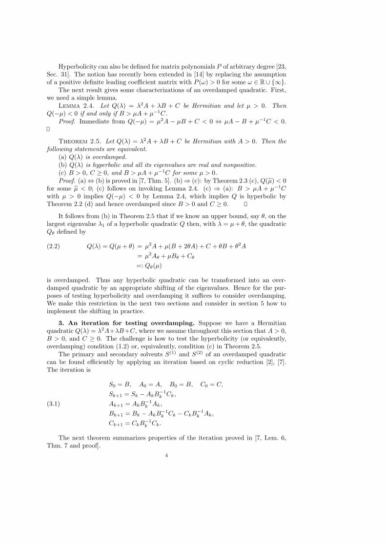
Hyperbolicity can also be defined for matrix polynomials P of arbitrary degree [23,Sec. 31]. The notion has recently been extended in [14] by replacing the assumptionof a positive definite leading coefficient matrix with P (ω) > 0 for some ω ∈ R∪ {∞}.
The next result gives some characterizations of an overdamped quadratic. First,we need a simple lemma.
Lemma 2.4. Let Q(λ) = λ2A + λB + C be Hermitian and let µ > 0. Then
Q(−µ) < 0 if and only if B > µA + µ−1C.
Proof. Immediate from Q(−µ) = µ2A − µB + C < 0 ⇔ µA − B + µ−1C < 0.
Theorem 2.5. Let Q(λ) = λ2A + λB + C be Hermitian with A > 0. Then the
following statements are equivalent.
(a) Q(λ) is overdamped.
(b) Q(λ) is hyperbolic and all its eigenvalues are real and nonpositive.
(c) B > 0, C ≥ 0, and B > µA + µ−1C for some µ > 0.Proof. (a) ⇔ (b) is proved in [7, Thm. 5]. (b) ⇒ (c): by Theorem 2.3 (c), Q(µ) < 0
for some µ < 0; (c) follows on invoking Lemma 2.4. (c) ⇒ (a): B > µA + µ−1Cwith µ > 0 implies Q(−µ) < 0 by Lemma 2.4, which implies Q is hyperbolic byTheorem 2.2 (d) and hence overdamped since B > 0 and C ≥ 0.
It follows from (b) in Theorem 2.5 that if we know an upper bound, say θ, on thelargest eigenvalue λ1 of a hyperbolic quadratic Q then, with λ = µ + θ, the quadraticQθ defined by
is overdamped. Thus any hyperbolic quadratic can be transformed into an over-damped quadratic by an appropriate shifting of the eigenvalues. Hence for the pur-poses of testing hyperbolicity and overdamping it suffices to consider overdamping.We make this restriction in the next two sections and consider in section 5 how toimplement the shifting in practice.
3. An iteration for testing overdamping. Suppose we have a Hermitianquadratic Q(λ) = λ2A+λB+C, where we assume throughout this section that A > 0,B > 0, and C ≥ 0. The challenge is how to test the hyperbolicity (or equivalently,overdamping) condition (1.2) or, equivalently, condition (c) in Theorem 2.5.
The primary and secondary solvents S(1) and S(2) of an overdamped quadraticcan be found efficiently by applying an iteration based on cyclic reduction [2], [7].The iteration is
S0 = B, A0 = A, B0 = B, C0 = C,
Sk+1 = Sk − AkB−1k Ck,
Ak+1 = AkB−1k Ak,(3.1)
Bk+1 = Bk − AkB−1k Ck − CkB−1
k Ak,
Ck+1 = CkB−1k Ck.
The next theorem summarizes properties of the iteration proved in [7, Lem. 6,Thm. 7 and proof].
4
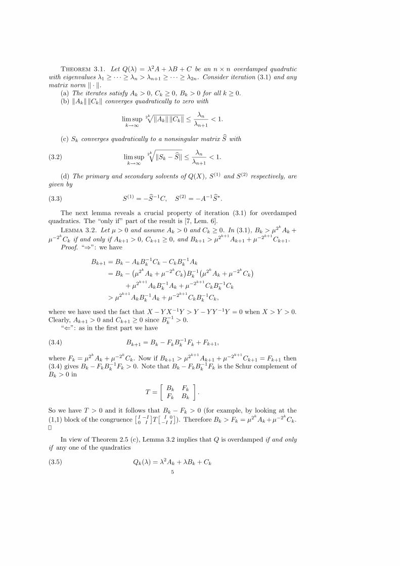
Theorem 3.1. Let Q(λ) = λ2A + λB + C be an n × n overdamped quadratic
with eigenvalues λ1 ≥ · · · ≥ λn > λn+1 ≥ · · · ≥ λ2n. Consider iteration (3.1) and any
matrix norm ‖ · ‖.(a) The iterates satisfy Ak > 0, Ck ≥ 0, Bk > 0 for all k ≥ 0.(b) ‖Ak‖‖Ck‖ converges quadratically to zero with
lim supk→∞
2k√‖Ak‖‖Ck‖ ≤
λn
λn+1< 1.
(c) Sk converges quadratically to a nonsingular matrix S with
lim supk→∞
2k
√‖Sk − S‖ ≤
λn
λn+1< 1.(3.2)
(d) The primary and secondary solvents of Q(X), S(1) and S(2) respectively, are
given by
S(1) = −S−1C, S(2) = −A−1S∗.(3.3)
The next lemma reveals a crucial property of iteration (3.1) for overdampedquadratics. The “only if” part of the result is [7, Lem. 6].
Lemma 3.2. Let µ > 0 and assume Ak > 0 and Ck ≥ 0. In (3.1), Bk > µ2k
Ak +
µ−2k
Ck if and only if Ak+1 > 0, Ck+1 ≥ 0, and Bk+1 > µ2k+1
Ak+1 + µ−2k+1
Ck+1.
Proof. “⇒”: we have
Bk+1 = Bk − AkB−1k Ck − CkB−1
k Ak
= Bk −(µ2k
Ak + µ−2k
Ck
)B−1
k
(µ2k
Ak + µ−2k
Ck
)
+ µ2k+1
AkB−1k Ak + µ−2k+1
CkB−1k Ck
> µ2k+1
AkB−1k Ak + µ−2k+1
CkB−1k Ck,
where we have used the fact that X − Y X−1Y > Y − Y Y −1Y = 0 when X > Y > 0.Clearly, Ak+1 > 0 and Ck+1 ≥ 0 since B−1
k > 0.“⇐”: as in the first part we have
Bk+1 = Bk − FkB−1k Fk + Fk+1,(3.4)
where Fk = µ2k
Ak + µ−2k
Ck. Now if Bk+1 > µ2k+1
Ak+1 + µ−2k+1
Ck+1 = Fk+1 then(3.4) gives Bk −FkB−1
k Fk > 0. Note that Bk −FkB−1k Fk is the Schur complement of
Bk > 0 in
T =
[Bk Fk
Fk Bk
].
So we have T > 0 and it follows that Bk − Fk > 0 (for example, by looking at the
(1,1) block of the congruence[
I0−II
]T
[I
−I0I
]). Therefore Bk > Fk = µ2k
Ak +µ−2k
Ck.
In view of Theorem 2.5 (c), Lemma 3.2 implies that Q is overdamped if and only
if any one of the quadratics
Qk(λ) = λ2Ak + λBk + Ck(3.5)
5
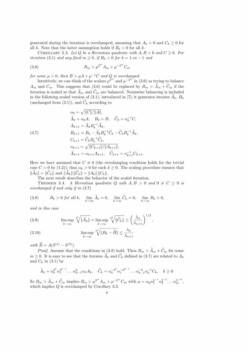
generated during the iteration is overdamped, assuming that Ak > 0 and Ck ≥ 0 forall k. Note that the latter assumption holds if Bk > 0 for all k.
Corollary 3.3. Let Q be a Hermitian quadratic with A,B > 0 and C ≥ 0. For
iteration (3.1) and any fixed m ≥ 0, if Bk > 0 for k = 1:m − 1 and
Bm > µ2m
Am + µ−2m
Cm(3.6)
for some µ > 0, then B > µA + µ−1C and Q is overdamped.
Intuitively, we can think of the scalars µ2m
and µ−2m
in (3.6) as trying to balance
Am and Cm. This suggests that (3.6) could be replaced by Bm > Am + Cm if the
iteration is scaled so that Am and Cm are balanced. Normwise balancing is includedin the following scaled version of (3.1), introduced in [7]; it generates iterates Ak, Bk
(unchanged from (3.1)), and Ck according to
α0 =√‖C‖/‖A‖,
A0 = α0A, B0 = B, C0 = α−10 C,
Ak+1 = AkB−1k Ak,
Bk+1 = Bk − AkB−1k Ck − CkB−1
k Ak,(3.7)
Ck+1 = CkB−1k Ck,
αk+1 =√‖Ck+1‖/‖Ak+1‖,
Ak+1 = αk+1Ak+1, Ck+1 = α−1k+1Ck+1.
Here we have assumed that C 6= 0 (the overdamping condition holds for the trivialcase C = 0 by (1.2)); thus αk > 0 for each k ≥ 0. The scaling procedure ensures that
‖Ak‖ = ‖Ck‖ and ‖Ak‖‖Ck‖ = ‖Ak‖‖Ck‖.The next result describes the behavior of the scaled iteration.Theorem 3.4. A Hermitian quadratic Q with A,B > 0 and 0 6= C ≥ 0 is
overdamped if and only if in (3.7)
Bk > 0 for all k, limk→∞
Ak = 0, limk→∞
Ck = 0, limk→∞
Bk > 0,(3.8)
and in this case
lim supk→∞
2k
√‖Ak‖ = lim sup
k→∞
2k
√‖Ck‖ ≤
(λn
λn+1
)1/2
,(3.9)
lim supk→∞
2k
√‖Bk − B‖ ≤
λn
λn+1(3.10)
with B = A(S(1) − S(2)).
Proof. Assume that the conditions in (3.8) hold. Then Bm > Am + Cm for some
m ≥ 0. It is easy to see that the iterates Ak and Ck defined in (3.7) are related to Ak
and Ck in (3.1) by
Ak = α2k
0 α2k−1
1 . . . α2k−1αkAk, Ck = α−2k
0 α−2k−1
1 . . . α−2k−1α
−1k Ck, k ≥ 0.
So Bm > Am + Cm implies Bm > µ2m
Am + µ−2m
Cm with µ = α0α2−1
1 α2−2
2 . . . α2−m
m ,which implies Q is overdamped by Corollary 3.3.
6
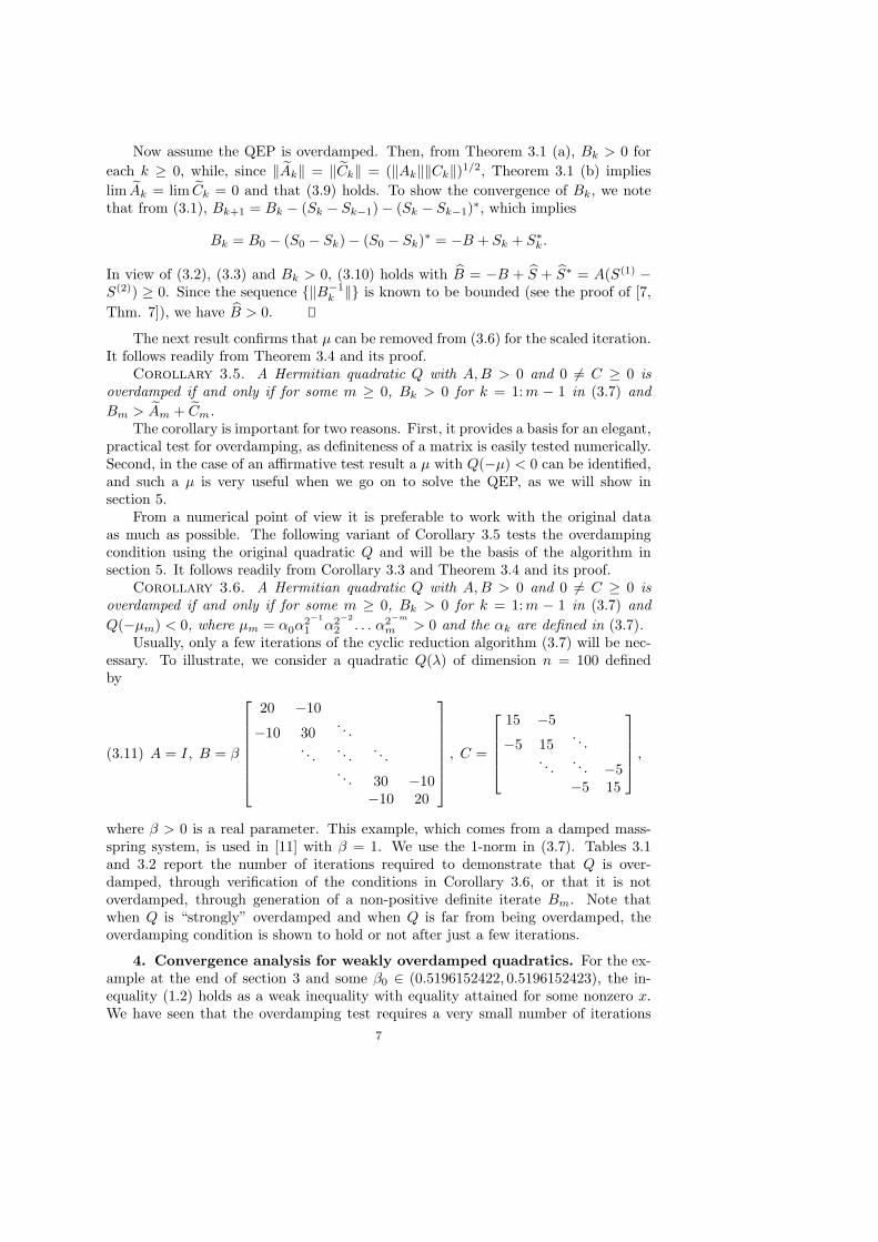
Now assume the QEP is overdamped. Then, from Theorem 3.1 (a), Bk > 0 for
each k ≥ 0, while, since ‖Ak‖ = ‖Ck‖ = (‖Ak‖‖Ck‖)1/2, Theorem 3.1 (b) implies
lim Ak = lim Ck = 0 and that (3.9) holds. To show the convergence of Bk, we notethat from (3.1), Bk+1 = Bk − (Sk − Sk−1) − (Sk − Sk−1)
∗, which implies
Bk = B0 − (S0 − Sk) − (S0 − Sk)∗ = −B + Sk + S∗k .
In view of (3.2), (3.3) and Bk > 0, (3.10) holds with B = −B + S + S∗ = A(S(1) −S(2)) ≥ 0. Since the sequence {‖B−1
k ‖} is known to be bounded (see the proof of [7,
Thm. 7]), we have B > 0.
The next result confirms that µ can be removed from (3.6) for the scaled iteration.It follows readily from Theorem 3.4 and its proof.
Corollary 3.5. A Hermitian quadratic Q with A,B > 0 and 0 6= C ≥ 0 is
overdamped if and only if for some m ≥ 0, Bk > 0 for k = 1:m − 1 in (3.7) and
Bm > Am + Cm.
The corollary is important for two reasons. First, it provides a basis for an elegant,practical test for overdamping, as definiteness of a matrix is easily tested numerically.Second, in the case of an affirmative test result a µ with Q(−µ) < 0 can be identified,and such a µ is very useful when we go on to solve the QEP, as we will show insection 5.
From a numerical point of view it is preferable to work with the original dataas much as possible. The following variant of Corollary 3.5 tests the overdampingcondition using the original quadratic Q and will be the basis of the algorithm insection 5. It follows readily from Corollary 3.3 and Theorem 3.4 and its proof.
Corollary 3.6. A Hermitian quadratic Q with A,B > 0 and 0 6= C ≥ 0 is
overdamped if and only if for some m ≥ 0, Bk > 0 for k = 1:m − 1 in (3.7) and
Q(−µm) < 0, where µm = α0α2−1
1 α2−2
2 . . . α2−m
m > 0 and the αk are defined in (3.7).Usually, only a few iterations of the cyclic reduction algorithm (3.7) will be nec-
essary. To illustrate, we consider a quadratic Q(λ) of dimension n = 100 definedby
A = I, B = β
20 −10
−10 30. . .
. . .. . .
. . .. . . 30 −10
−10 20
, C =
15 −5
−5 15. . .
. . .. . . −5−5 15
,(3.11)
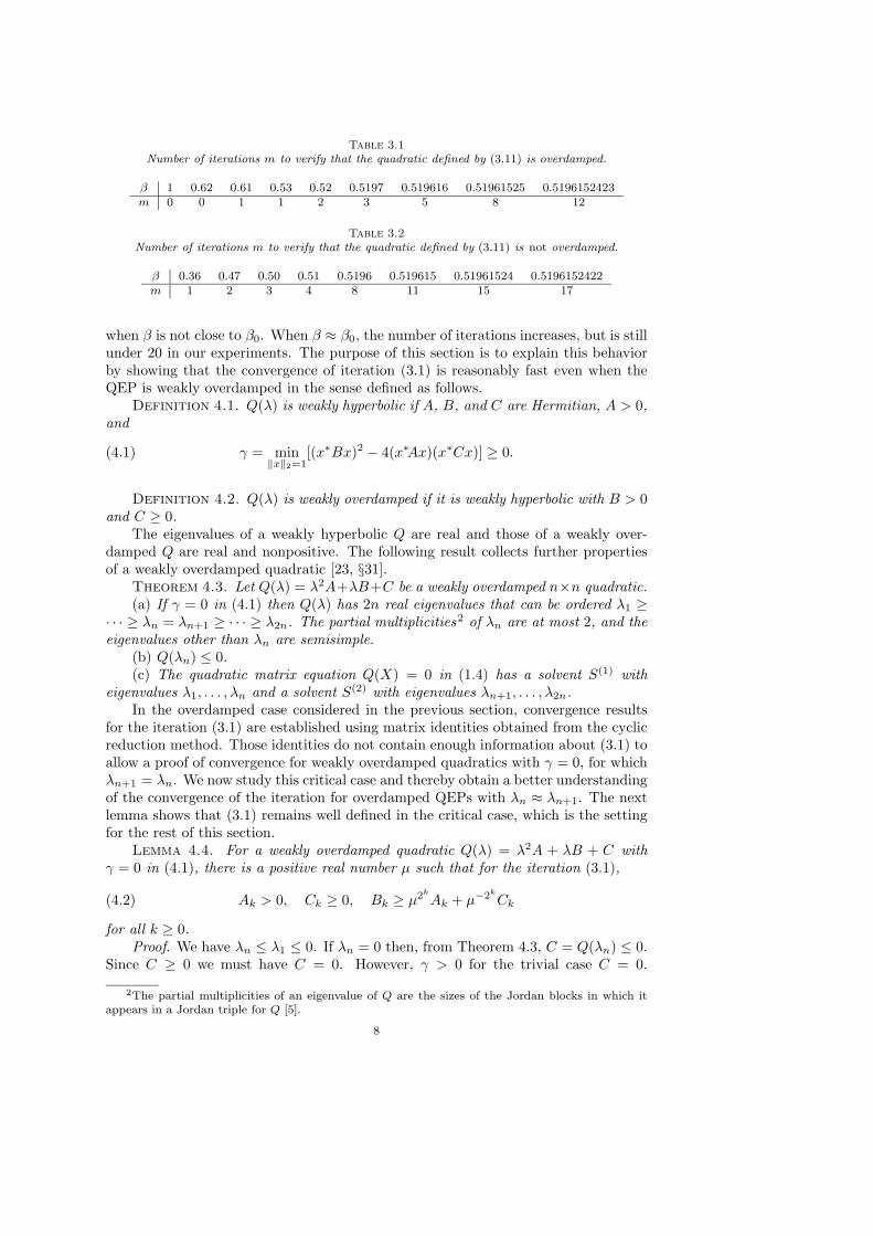
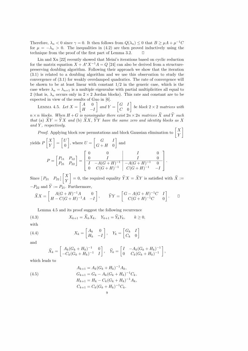
where β > 0 is a real parameter. This example, which comes from a damped mass-spring system, is used in [11] with β = 1. We use the 1-norm in (3.7). Tables 3.1and 3.2 report the number of iterations required to demonstrate that Q is over-damped, through verification of the conditions in Corollary 3.6, or that it is notoverdamped, through generation of a non-positive definite iterate Bm. Note thatwhen Q is “strongly” overdamped and when Q is far from being overdamped, theoverdamping condition is shown to hold or not after just a few iterations.
4. Convergence analysis for weakly overdamped quadratics. For the ex-ample at the end of section 3 and some β0 ∈ (0.5196152422, 0.5196152423), the in-equality (1.2) holds as a weak inequality with equality attained for some nonzero x.We have seen that the overdamping test requires a very small number of iterations
7
Table 3.1Number of iterations m to verify that the quadratic defined by (3.11) is overdamped.
when β is not close to β0. When β ≈ β0, the number of iterations increases, but is stillunder 20 in our experiments. The purpose of this section is to explain this behaviorby showing that the convergence of iteration (3.1) is reasonably fast even when theQEP is weakly overdamped in the sense defined as follows.
Definition 4.1. Q(λ) is weakly hyperbolic if A, B, and C are Hermitian, A > 0,and
γ = min‖x‖2=1
[(x∗Bx)2 − 4(x∗Ax)(x∗Cx)] ≥ 0.(4.1)
Definition 4.2. Q(λ) is weakly overdamped if it is weakly hyperbolic with B > 0and C ≥ 0.
The eigenvalues of a weakly hyperbolic Q are real and those of a weakly over-damped Q are real and nonpositive. The following result collects further propertiesof a weakly overdamped quadratic [23, §31].
Theorem 4.3. Let Q(λ) = λ2A+λB+C be a weakly overdamped n×n quadratic.
(a) If γ = 0 in (4.1) then Q(λ) has 2n real eigenvalues that can be ordered λ1 ≥· · · ≥ λn = λn+1 ≥ · · · ≥ λ2n. The partial multiplicities2 of λn are at most 2, and the
eigenvalues other than λn are semisimple.
(b) Q(λn) ≤ 0.(c) The quadratic matrix equation Q(X) = 0 in (1.4) has a solvent S(1) with
eigenvalues λ1, . . . , λn and a solvent S(2) with eigenvalues λn+1, . . . , λ2n.
In the overdamped case considered in the previous section, convergence resultsfor the iteration (3.1) are established using matrix identities obtained from the cyclicreduction method. Those identities do not contain enough information about (3.1) toallow a proof of convergence for weakly overdamped quadratics with γ = 0, for whichλn+1 = λn. We now study this critical case and thereby obtain a better understandingof the convergence of the iteration for overdamped QEPs with λn ≈ λn+1. The nextlemma shows that (3.1) remains well defined in the critical case, which is the settingfor the rest of this section.
Lemma 4.4. For a weakly overdamped quadratic Q(λ) = λ2A + λB + C with
γ = 0 in (4.1), there is a positive real number µ such that for the iteration (3.1),
Ak > 0, Ck ≥ 0, Bk ≥ µ2k
Ak + µ−2k
Ck(4.2)
for all k ≥ 0.Proof. We have λn ≤ λ1 ≤ 0. If λn = 0 then, from Theorem 4.3, C = Q(λn) ≤ 0.
Since C ≥ 0 we must have C = 0. However, γ > 0 for the trivial case C = 0.
2The partial multiplicities of an eigenvalue of Q are the sizes of the Jordan blocks in which itappears in a Jordan triple for Q [5].
8
Therefore, λn < 0 since γ = 0. It then follows from Q(λn) ≤ 0 that B ≥ µA + µ−1Cfor µ = −λn > 0. The inequalities in (4.2) are then proved inductively using thetechnique from the proof of the first part of Lemma 3.2.
Lin and Xu [22] recently showed that Meini’s iterations based on cyclic reductionfor the matrix equation X + A∗X−1A = Q [24] can also be derived from a structure-preserving doubling algorithm. Following their approach we show that the iteration(3.1) is related to a doubling algorithm and we use this observation to study theconvergence of (3.1) for weakly overdamped quadratics. The rate of convergence willbe shown to be at least linear with constant 1/2 in the generic case, which is thecase where λn = λn+1 is a multiple eigenvalue with partial multiplicities all equal to2 (that is, λn occurs only in 2 × 2 Jordan blocks). This rate and constant are to beexpected in view of the results of Guo in [6].
Lemma 4.5. Let X =
[A 0H −I
]and Y =
[G IC 0
]be block 2 × 2 matrices with
n×n blocks. When H + G is nonsingular there exist 2n× 2n matrices X and Y such
that (a) XY = Y X and (b) XX, Y Y have the same zero and identity blocks as Xand Y , respectively.
Proof. Applying block row permutations and block Gaussian elimination to
[XY
]
yields P
[XY
]=
[U0
], where U =
[G I
G + H 0
]and
P =
[P11 P12
P21 P22
]=
0 0 I 00 I I 0I −A(G + H)−1 −A(G + H)−1 00 C(G + H)−1 C(G + H)−1 −I
.
Since [P21 P22 ]
[XY
]= 0, the required equality Y X = XY is satisfied with X :=
−P22 and Y := P21. Furthermore,
XX =
[A(G + H)−1A 0
H − C(G + H)−1A −I
], Y Y =
[G − A(G + H)−1C I
C(G + H)−1C 0
].
Lemma 4.5 and its proof suggest the following recurrence
Xk+1 = XkXk, Yk+1 = YkYk, k ≥ 0,(4.3)
with
Xk =
[Ak 0Hk −I
], Yk =
[Gk ICk 0
](4.4)
and
Xk =
[Ak(Gk + Hk)−1 0−Ck(Gk + Hk)−1 I
], Yk =
[I −Ak(Gk + Hk)−1
0 Ck(Gk + Hk)−1
],
which leads to
Ak+1 = Ak(Gk + Hk)−1Ak,
Gk+1 = Gk − Ak(Gk + Hk)−1Ck,(4.5)
Hk+1 = Hk − Ck(Gk + Hk)−1Ak,
Ck+1 = Ck(Gk + Hk)−1Ck.
9
With
A0 = A, C0 = C, G0 = 0, H0 = B(4.6)
the iteration (3.1) is recovered from (4.5) by letting Bk = Gk + Hk and Sk = H∗k . By
Lemma 4.4, Bk > 0 for all k ≥ 0. Therefore with the starting matrices (4.6), iteration(4.5) is well defined. Note that Xk in (4.4) is nonsingular for all k ≥ 0 and, from (4.3)
and the property that XkYk = YkXk,
X−1k+1Yk+1 = (XkXk)−1YkYk = X−1
k X−1k YkYk = X−1
k YkX−1k Yk = (X−1
k Yk)2.(4.7)
It follows from (4.7) that for all k ≥ 0,
X−1k Yk =
(X−1
0 Y0
)2k
.(4.8)
The identity (4.8) is what we need to prove the convergence of (4.5) with (4.6) andhence the convergence of (3.1).
The next result describes the convergence behavior in the generic case.Theorem 4.6. Let Q(λ) be weakly overdamped with eigenvalues λ1 ≥ · · · ≥ λn =
λn+1 ≥ · · · ≥ λ2n and assume that the partial multiplicities of λn are all equal to 2.Let S(1) and S(2) be the primary and secondary solvents of Q(X) = 0, respectively,
and assume that λn is a semisimple eigenvalue of S(1) and S(2). Then the iterates
Gk, Hk, Ak, and Ck defined by (4.5) and (4.6) satisfy
lim supk→∞
k
√‖Gk − AS(1)‖ ≤
1
2, lim sup
k→∞
k
√‖Hk + AS(2)‖ ≤
1
2,
lim supk→∞
k
√‖Ak‖‖Ck‖ ≤
1
4.
Proof. We start by making the change of variables (or scaling) λ = µθ, where
θ = |λn| > 0 (see the proof of Lemma 4.4) so that µn = µn+1 = −1 and define Q(µ) =
µ2A + µB + C with (A, B, C) = (θA,B, θ−1C). For this triple denote the iterates of
(4.5) by Ak, Gk, Hk, Ck. It is easy to see that for all k ≥ 0, Gk = Gk, Hk = Hk,
Ak = θ2k
Ak, and Ck = θ−2k
Ck, so that ‖Ak‖‖Ck‖ = ‖Ak‖‖Ck‖. The primary and
secondary solvents of AS2 + BS + C = 0 are S(1) = θ−1S(1) and S(2) = θ−1S(2),respectively. Note that AS(i) = AS(i), i = 1, 2. To avoid notational clutter, we omitthe hats on matrices in the rest of the proof.
We now consider the iterations for the block 2 × 2 matrices Xk and Yk in (4.4).With A0 = A, C0 = C, G0 = 0, and H0 = B, the pencil
µX0 + Y0 = µ
[A 0B −In
]+
[0 In
C 0
](4.9)
is a linearization of Q(µ) [5]. Hence −X−10 Y0 and Q(µ) have the same eigenvalues, with
the same partial multiplicities. Suppose there are r 2 × 2 Jordan blocks associatedwith eigenvalues equal to µn = −1, where r ≥ 1 by assumption. Rearranging theJordan canonical form of X−1
0 Y0 appropriately yields
V −1(X−10 Y0)V =
[D2 ⊕ Ir 0 ⊕ Ir
0 D1 ⊕ Ir
]=: DV ,(4.10)
W−1(X−10 Y0)W =
[D2 ⊕ Ir 00 ⊕ Ir D1 ⊕ Ir
]=: DW ,(4.11)
10
where V and W are nonsingular, D1 and D2 are (n − r) × (n − r) diagonal matricescontaining the (semisimple) eigenvalues less than 1 and greater than 1 in modulus,respectively, and M ⊕ N denotes
[M0
0N
]. Now partition V and W as block 2 × 2
matrices with n × n blocks:
V =
[V1 V3
V2 V4
], W =
[W1 W3
W2 W4
],
and note that from (4.10)–(4.11),
X−10 Y0
[V1
V2
]=
[V1
V2
](D2 ⊕ Ir), X−1
0 Y0
[W3
W4
]=
[W3
W4
](D1 ⊕ Ir).(4.12)
By Theorem 4.3 and our assumption on S(1) and S(2) there exist nonsingular U1 andU2 such that
−S(1) = U1(D1 ⊕ Ir)U−11 , −S(2) = U2(D2 ⊕ Ir)U
−12 .(4.13)
Since S(i), i = 1, 2, is a solution of Q(X) = 0, from (4.9) we obtain
X−10 Y0
[In
−AS(i)
]=
[In
−AS(i)
](−S(i)), i = 1, 2.
On comparing with the invariant subspaces in (4.12) and using (4.13) we deduce that
[V1
V2
]=
[U2
−AS(2)U2
]Z1,
[W3
W4
]=
[U1
−AS(1)U1
]Z2,
with Z1 and Z2 nonsingular, where we have also used the fact that there are exactlyr eigenvectors of X−1
0 Y0 corresponding to the eigenvalue 1. Hence V1 and W3 arenonsingular and
−AS(2) = V2V−11 , −AS(1) = W4W
−13 .(4.14)
By (4.8)–(4.11) we have V −1(X−1k Yk)V = D2k
V and W−1(X−1k Yk)W = D2k
W , so that
YkV = XkV D2k
V , YkW = XkWD2k
W .(4.15)
On equating blocks using (4.4) this yields
GkV1 + V2 = AkV1(D2k
2 ⊕ Ir),(4.16)
GkV3 + V4 = AkV1(0 ⊕ 2kIr) + AkV3(D2k
1 ⊕ Ir),(4.17)
CkV1 = (HkV1 − V2)(D2k
2 ⊕ Ir),(4.18)
CkV3 = (HkV1 − V2)(0 ⊕ 2kIr) + (HkV3 − V4)(D2k
1 ⊕ Ir)(4.19)
and
GkW1 + W2 = AkW1(D2k
2 ⊕ Ir) + AkW3(0 ⊕ 2kIr),(4.20)
GkW3 + W4 = AkW3(D2k
1 ⊕ Ir),(4.21)
CkW1 = (HkW1 − W2)(D2k
2 ⊕ Ir) + (HkW3 − W4)(0 ⊕ 2kIr),(4.22)
CkW3 = (HkW3 − W4)(D2k
1 ⊕ Ir).(4.23)
11
By (4.22) and (4.23) we have
Ck(W3−W1(0⊕2−kIr)) = (HkW3−W4)(D2k
1 ⊕0)−(HkW1−W2)(0⊕2−kIr).(4.24)
By (4.18) we have
Hk = V2V−11 + CkV1(D
−2k
2 ⊕ Ir)V−11 .(4.25)
Inserting (4.25) in (4.24), we obtain
Ck
(W3 − W1(0 ⊕ 2−kIr) − V1(D
−2k
2 ⊕ Ir)V−11
(W3(D
2k
1 ⊕ 0) − W1(0 ⊕ 2−kIr)))
= (V2V−11 W3 − W4)(D
2k
1 ⊕ 0) − (V2V−11 W1 − W2)(0 ⊕ 2−kIr),
from which it follows, since D1 and D2 are diagonal with diagonal elements of mag-nitude less than 1 and greater than 1, respectively, that
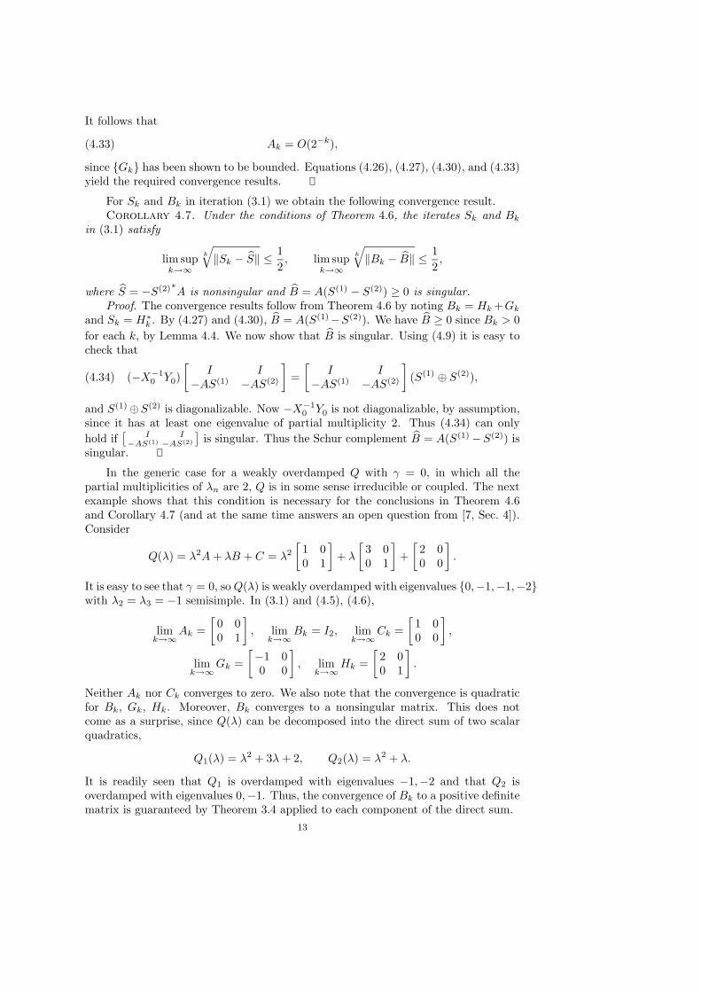
since {Gk} has been shown to be bounded. Equations (4.26), (4.27), (4.30), and (4.33)yield the required convergence results.
For Sk and Bk in iteration (3.1) we obtain the following convergence result.Corollary 4.7. Under the conditions of Theorem 4.6, the iterates Sk and Bk
in (3.1) satisfy
lim supk→∞
k
√‖Sk − S‖ ≤
1
2, lim sup
k→∞
k
√‖Bk − B‖ ≤
1
2,
where S = −S(2)∗A is nonsingular and B = A(S(1) − S(2)) ≥ 0 is singular.
Proof. The convergence results follow from Theorem 4.6 by noting Bk = Hk +Gk
and Sk = H∗k . By (4.27) and (4.30), B = A(S(1)−S(2)). We have B ≥ 0 since Bk > 0
for each k, by Lemma 4.4. We now show that B is singular. Using (4.9) it is easy tocheck that
(−X−10 Y0)
[I I
−AS(1) −AS(2)
]=
[I I
−AS(1) −AS(2)
](S(1) ⊕ S(2)),(4.34)
and S(1) ⊕S(2) is diagonalizable. Now −X−10 Y0 is not diagonalizable, by assumption,
since it has at least one eigenvalue of partial multiplicity 2. Thus (4.34) can only
hold if[
I−AS(1)
I−AS(2)
]is singular. Thus the Schur complement B = A(S(1) −S(2)) is
singular.
In the generic case for a weakly overdamped Q with γ = 0, in which all thepartial multiplicities of λn are 2, Q is in some sense irreducible or coupled. The nextexample shows that this condition is necessary for the conclusions in Theorem 4.6and Corollary 4.7 (and at the same time answers an open question from [7, Sec. 4]).Consider
Q(λ) = λ2A + λB + C = λ2
[1 00 1
]+ λ
[3 00 1
]+
[2 00 0
].
It is easy to see that γ = 0, so Q(λ) is weakly overdamped with eigenvalues {0,−1,−1,−2}with λ2 = λ3 = −1 semisimple. In (3.1) and (4.5), (4.6),
limk→∞
Ak =
[0 00 1
], lim
k→∞Bk = I2, lim
k→∞Ck =
[1 00 0
],
limk→∞
Gk =
[−1 00 0
], lim
k→∞Hk =
[2 00 1
].
Neither Ak nor Ck converges to zero. We also note that the convergence is quadraticfor Bk, Gk, Hk. Moreover, Bk converges to a nonsingular matrix. This does notcome as a surprise, since Q(λ) can be decomposed into the direct sum of two scalarquadratics,
Q1(λ) = λ2 + 3λ + 2, Q2(λ) = λ2 + λ.
It is readily seen that Q1 is overdamped with eigenvalues −1,−2 and that Q2 isoverdamped with eigenvalues 0,−1. Thus, the convergence of Bk to a positive definitematrix is guaranteed by Theorem 3.4 applied to each component of the direct sum.
13
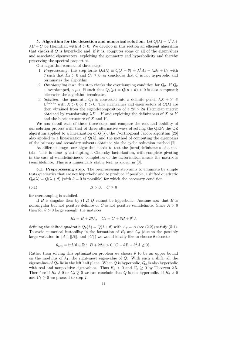
5. Algorithm for the detection and numerical solution. Let Q(λ) = λ2A+λB + C be Hermitian with A > 0. We develop in this section an efficient algorithmthat checks if Q is hyperbolic and, if it is, computes some or all of the eigenvaluesand associated eigenvectors, exploiting the symmetry and hyperbolicity and therebypreserving the spectral properties.
Our algorithm consists of three steps:1. Preprocessing : this step forms Qθ(λ) ≡ Q(λ + θ) = λ2Aθ + λBθ + Cθ with
θ such that Bθ > 0 and Cθ ≥ 0, or concludes that Q is not hyperbolic andterminates the algorithm.
2. Overdamping test : this step checks the overdamping condition for Qθ. If Qθ
is overdamped, a µ ∈ R such that Qθ(µ) = Q(µ + θ) < 0 is also computed;otherwise the algorithm terminates.
3. Solution: the quadratic Qθ is converted into a definite pencil λX + Y ∈C
2n×2n with X > 0 or Y > 0. The eigenvalues and eigenvectors of Q(λ) arethen obtained from the eigendecomposition of a 2n × 2n Hermitian matrixobtained by transforming λX + Y and exploiting the definiteness of X or Yand the block structure of X and Y .
We now detail each of these three steps and compare the cost and stability ofour solution process with that of three alternative ways of solving the QEP: the QZalgorithm applied to a linearization of Q(λ), the J-orthogonal Jacobi algorithm [26]also applied to a linearization of Q(λ), and the method of computing the eigenpairsof the primary and secondary solvents obtained via the cyclic reduction method [7].
At different stages our algorithm needs to test the (semi)definiteness of a ma-trix. This is done by attempting a Cholesky factorization, with complete pivotingin the case of semidefinitiness: completion of the factorization means the matrix is(semi)definite. This is a numerically stable test, as shown in [8].
5.1. Preprocessing step. The preprocessing step aims to eliminate by simpletests quadratics that are not hyperbolic and to produce, if possible, a shifted quadraticQθ(λ) = Q(λ + θ) (with θ = 0 is possible) for which the necessary condition
B > 0, C ≥ 0(5.1)
for overdamping is satisfied.If B is singular then by (1.2) Q cannot be hyperbolic. Assume now that B is
nonsingular but not positive definite or C is not positive semidefinite. Since A > 0then for θ > 0 large enough, the matrices
Bθ = B + 2θA, Cθ = C + θB + θ2A
defining the shifted quadratic Qθ(λ) = Q(λ+ θ) with Aθ = A (see (2.2)) satisfy (5.1).To avoid numerical instability in the formation of Bθ and Cθ (due to the possiblylarge variation in ‖A‖, ‖B‖, and ‖C‖) we would ideally like to choose θ close to
θopt = inf{θ ∈ R : B + 2θA > 0, C + θB + θ2A ≥ 0}.
Rather than solving this optimization problem we choose θ to be an upper boundon the modulus of λ1, the right-most eigenvalue of Q. With such a shift, all theeigenvalues of Qθ lie in the left half plane. When Q is hyperbolic, Qθ is also hyperbolicwith real and nonpositive eigenvalues. Thus Bθ > 0 and Cθ ≥ 0 by Theorem 2.5.Therefore if Bθ 6> 0 or Cθ 6≥ 0 we can conclude that Q is not hyperbolic. If Bθ > 0and Cθ ≥ 0 we proceed to step 2.
14
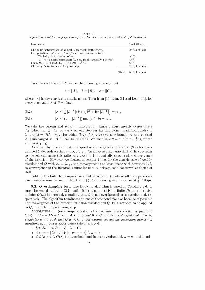
Table 5.1Operation count for the preprocessing step. Matrices are assumed real and of dimension n.
Operations Cost (flops)
Cholesky factorization of B and C to check definiteness. 2n3/3 or lessComputation of θ when B and/or C not positive definite:
Cholesky factorization of A. n3/3‖A−1‖ (1-norm estimation [9, Sec. 15.3], typically 4 solves). 4n2
Form Bθ = B + 2θA, Cθ = C + θB + θ2A. 6n2
Cholesky factorizations of Bθ and Cθ. 2n3/3 or less
Total 5n3/3 or less
To construct the shift θ we use the following strategy. Let
a = ‖A‖, b = ‖B‖, c = ‖C‖,
where ‖ · ‖ is any consistent matrix norm. Then from [16, Lem. 3.1 and Lem. 4.1], forevery eigenvalue λ of Q we have
|λ| ≤1
2‖A−1‖
(b +
√b2 + 4c/‖A−1‖
)=: σ1,(5.2)
|λ| ≤(1 + ‖A−1‖
)max(c1/2, b) =: σ2.(5.3)
We take the 1-norm and set σ = min(σ1, σ2). Since σ must greatly overestimate|λ1| when |λn| ≫ |λ1| we carry on one step further and form the shifted quadraticQ−σ/2(λ) = Q(λ − σ/2) for which (5.2)–(5.3) give two new bounds τ1 and τ2 (and
A is unchanged so ‖A−1‖ can be re-used). We then take θ = min(σ, τ − 12σ), where
τ = min(τ1, τ2).As shown by Theorem 3.4, the speed of convergence of iteration (3.7) for over-
damped Q depends on the ratio λn/λn+1. An unnecessarily large shift of the spectrumto the left can make this ratio very close to 1, potentially causing slow convergenceof the iteration. However, we showed in section 4 that for the generic case of weaklyoverdamped Q with λn = λn+1 the convergence is at least linear with constant 1/2,so convergence of the iteration cannot be unduly delayed by a conservative choice ofshift.
Table 5.1 details the computations and their cost. (Costs of all the operationsused here are summarized in [10, App. C].) Preprocessing requires at most 5
3n3 flops.
5.2. Overdamping test. The following algorithm is based on Corollary 3.6. Itruns the scaled iteration (3.7) until either a non-positive definite Bk or a negativedefinite Q(µk) is detected, signalling that Q is not overdamped or is overdamped, re-spectively. The algorithm terminates on one of these conditions or because of possiblenon-convergence of the iteration for a non-overdamped Q. It is intended to be appliedto Qθ from the preprocessing step.
Algorithm 5.1 (overdamping test). This algorithm tests whether a quadratic
Q(λ) = λ2A + λB + C with A,B > 0 and 0 6= C ≥ 0 is overdamped and, if it is,
computes µ < 0 such that Q(µ) < 0. Input parameters are the maximum number of
iterations kmax and a convergence tolerance ǫ > 0.1 Set A0 = A, B0 = B, C0 = C.
2 Set α0 = ‖C0‖1/‖A0‖1, µ0 = −α1/20 , k = 0.
3 if Q(µ0) < 0, Q(λ) is (hyperbolic and hence) overdamped, µ = µ0, quit, end
15
4 while k < kmax
5 Bk+1 = Bk − AkB−1k Ck − CkB−1
k Ak
6 if ‖Bk+1 − Bk‖1/‖Bk+1‖1 ≤ ǫ, goto line 15, end7 if Bk+1 6> 0, Q is not overdamped, quit, end8 Ak+1 = αkAkB−1
k Ak
9 Ck+1 = α−1k CkB−1
k Ck
10 αk+1 = ‖Ck+1‖1/‖Ak+1‖1
11 µk+1 = µkα1/2k+2
k+1
12 if Q(µk+1) < 0, Q is overdamped, µ = µk+1, quit, end13 k = k + 114 end15 Q is not overdamped. % See the discussion below.Note that the crucial definiteness test on line 12 of Algorithm 5.1 is carried out
on Q and not on Qk in (3.5). Hence a positive test can be interpreted irrespectiveof rounding errors in the iteration: the only errors are in forming Q(µk+1) and incomputing its Cholesky factor. For a non-overdamped Q, it is possible that Bk > 0for all k (see the example at the end of section 4). However, if convergence of theBk is detected on line 6 then Q is declared not overdamped because by this point anoverdamped Q would have been detected, while if kmax is large enough (say kmax = 20)and this iteration limit is reached then Q can reasonably be declared not overdampedin view of the fast (quadratic) convergence of (3.7) for an overdamped Q.
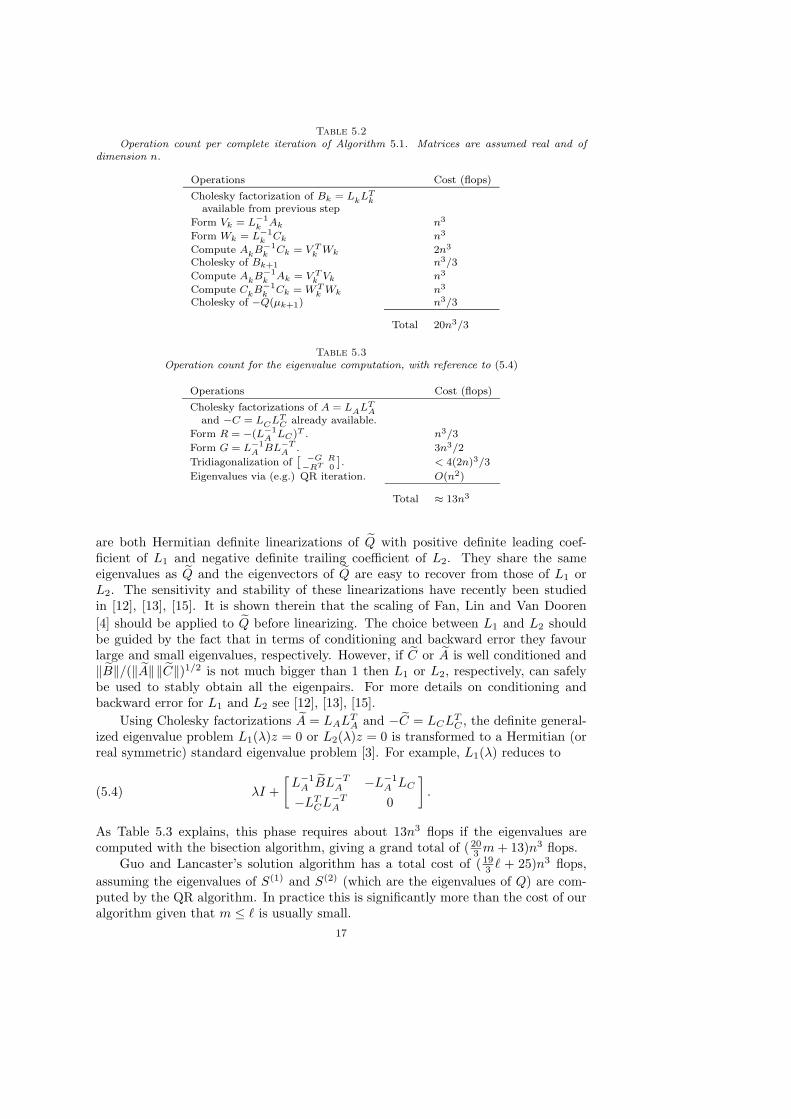
The implementation details of Algorithm 5.1 and the cost per iteration are de-scribed in Table 5.2. The total cost for m iterations is 1
3n3 flops for m = 0 and roughly203 mn3 flops for m ≥ 1.
Guo and Lancaster’s test for overdamping is based on iteration (3.1), scaled as
in (3.7). For the computation of S, 193 ℓn3 flops are required where ℓ is the number of
iterations for convergence of (3.1). An extra 5n3 flops is needed to form the two sol-vents S(1) and S(2) (which are nonsymmetric in general) via (3.3). Then the smallesteigenvalue λn of S(1) and the largest eigenvalue λn+1 of S(2) need to be computedand the definiteness of Q((λn + λn+1)/2) tested. The total cost is ( 19
3 ℓ + 163 )n3 flops
plus the cost of finding λn and λn+1. Since m ≤ ℓ, Algorithm 5.1 is clearly the moreefficient, possibly significantly so.
Another way to test overdamping is to apply the J-orthogonal Jacobi algorithmof Veselic [26] to a particular symmetric linearization of Q(λ), since the algorithmbreaks down when applied to an indefinite pair. Note that this algorithm uses hyper-bolic transformations and so is potentially unstable. The algorithm must be run tocompletion to check whether the problem is overdamped, and upon completion it hascomputed the eigenvalues. It requires an initial 11
3 n3 flops followed by 12sn3 flops,where s is the number of sweeps performed.
5.3. Solving hyperbolic QEPs via definite linearizations. Recall that thescalar µ computed by Algorithm 5.1 applied to Qθ is such that Q(µ+θ) = Qθ(µ) < 0.Hence with ω = µ + θ we have
Q(t) = Q(t + ω) = t2A + t(B + 2ωA) + C + ωB + ω2A
= t2A + tB + C,
with C = Q(ω) < 0 and A = A > 0. The pencils
L1(λ) = λ
[A 00 −C
]+
[B CC 0
], L2(λ) = λ
[0 AA B
]+
[−A 00 C
]
16
Table 5.2Operation count per complete iteration of Algorithm 5.1. Matrices are assumed real and of
dimension n.
Operations Cost (flops)
Cholesky factorization of Bk = LkLT
k
available from previous step
Form Vk = L−1
kAk n3
Form Wk = L−1
kCk n3
Compute AkB−1
kCk = V T
kWk 2n3
Cholesky of Bk+1 n3/3
Compute AkB−1
kAk = V T
kVk n3
Compute CkB−1
kCk = W T
kWk n3
Cholesky of −Q(µk+1) n3/3
Total 20n3/3
Table 5.3Operation count for the eigenvalue computation, with reference to (5.4)
Operations Cost (flops)
Cholesky factorizations of A = LA
LT
A
and −C = LC
LT
Calready available.
Form R = −(L−1
ALC)T . n3/3
Form G = L−1
ABL−T
A. 3n3/2
Tridiagonalization ofˆ −G
−RT
R
0
˜
. < 4(2n)3/3
Eigenvalues via (e.g.) QR iteration. O(n2)
Total ≈ 13n3
are both Hermitian definite linearizations of Q with positive definite leading coef-ficient of L1 and negative definite trailing coefficient of L2. They share the sameeigenvalues as Q and the eigenvectors of Q are easy to recover from those of L1 orL2. The sensitivity and stability of these linearizations have recently been studiedin [12], [13], [15]. It is shown therein that the scaling of Fan, Lin and Van Dooren
[4] should be applied to Q before linearizing. The choice between L1 and L2 shouldbe guided by the fact that in terms of conditioning and backward error they favourlarge and small eigenvalues, respectively. However, if C or A is well conditioned and‖B‖/(‖A‖‖C‖)1/2 is not much bigger than 1 then L1 or L2, respectively, can safelybe used to stably obtain all the eigenpairs. For more details on conditioning andbackward error for L1 and L2 see [12], [13], [15].
Using Cholesky factorizations A = LALTA and −C = LCLT
C , the definite general-ized eigenvalue problem L1(λ)z = 0 or L2(λ)z = 0 is transformed to a Hermitian (orreal symmetric) standard eigenvalue problem [3]. For example, L1(λ) reduces to
λI +
[L−1
A BL−TA −L−1
A LC
−LTCL−T
A 0
].(5.4)
As Table 5.3 explains, this phase requires about 13n3 flops if the eigenvalues arecomputed with the bisection algorithm, giving a grand total of (20
3 m + 13)n3 flops.Guo and Lancaster’s solution algorithm has a total cost of (19
3 ℓ + 25)n3 flops,
assuming the eigenvalues of S(1) and S(2) (which are the eigenvalues of Q) are com-puted by the QR algorithm. In practice this is significantly more than the cost of ouralgorithm given that m ≤ ℓ is usually small.
17
The most common way of solving the QEP is to apply the QZ algorithm or aKrylov method to a linearization L of Q. The QZ algorithm applied to the 2n × 2nL costs 240n3 flops for the computation of the eigenvalues.
Our algorithm has two important advantages over that of Guo and Lancasterand QZ applied to a linearization, besides its more favorable operation count. First,it work entirely with symmetric matrices, which reduces the storage requirement.Second, it guarantees to produce real eigenvalues in floating point arithmetic; theother two approaches cannot do so because they invoke the QZ algorithm and thenonsymmetric QR algorithm.
6. Numerical experiment. We describe an experiment that illustrates the be-havior of our algorithm for testing overdamping. More extensive testing of this algo-rithm, and of the preprocessing and solve procedures described in section 5, will bepresented in a future publication. Our experiments were performed in MATLAB 7.4(R2007a), for which the unit roundoff is u = 2−53 ≈ 1.1 × 10⁻¹⁶. We took kmax = 30and ǫ = u in Algorithm 5.1.
We first describe a useful technique for generating symmetric quadratic matrixpolynomials with prescribed eigenvalues and eigenvectors and positive definite coeffi-cient matrices.
Let (λk, vk), k = 1: 2n be a set of given real eigenpairs such that with
Then the symmetric quadratic polynomial defined by the matrices
A = Γ−1, B = −A(V1Λ21V
T1 − V2Λ
22V
T2 )A,(6.2a)
C = −A(V1Λ31V
T1 − V2Λ
32V
T2 )A + BΓB,(6.2b)
has eigenpairs (λk, vk), k = 1: 2n (see [21] for example). We now show how to generatea potentially overdamped quadratic.
Lemma 6.1. Assume that 0 > λ1 ≥ · · · ≥ λn > λn+1 ≥ · · · ≥ λ2n. Then Γ is
nonsingular and the matrices generated by (6.2) satisfy A > 0, B > 0, and C > 0.Proof. It follows from Weyl’s theorem [18, p. 181] that Γ > 0 and hence that
A > 0. All matrices V2 that satisfy the first constraint in (6.1) can be written V1Ufor some orthogonal U . Hence we can write
B = −AV1(Λ21 − UΛ2
2UT )V T
1 A ≡ −AV1(H21 − H2
2 )V T1 A,
where H1 = Λ1 and H2 = UΛ2UT , and again Weyl’s theorem guarantees that B > 0.
It is known that (V,Λ, PV T ) where P = diag(In,−In) forms a self adjoint triplefor Q(λ) [5, Sec. 10.2]. Since Q has no zero eigenvalues, C is nonsingular and a formulafor its inverse is easily obtained from the resolvent form of Q(λ): for λ 6= λi,
Q(λ)−1 = V (λI2n − Λ)−1PV T .
Setting λ = 0 in the above expression gives
C−1 = −V Λ−1PV T = −V1(H−11 − H−1
2 )V T1
18
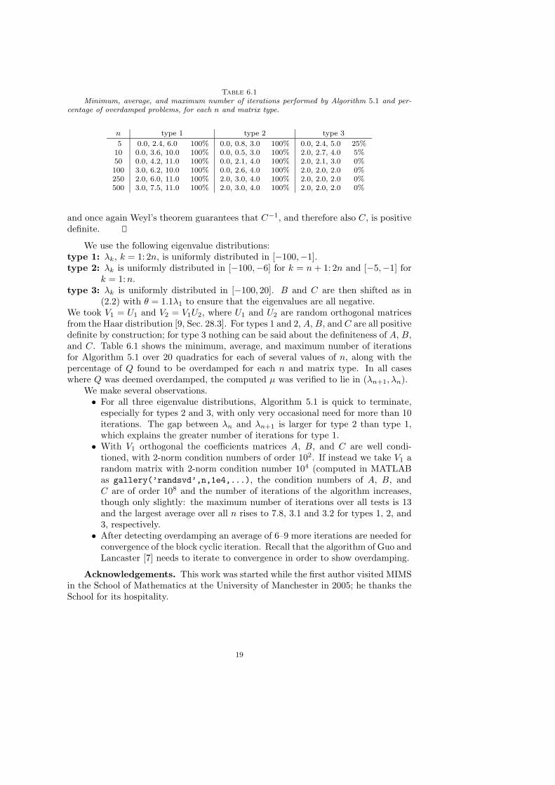
Table 6.1Minimum, average, and maximum number of iterations performed by Algorithm 5.1 and per-
centage of overdamped problems, for each n and matrix type.
and once again Weyl’s theorem guarantees that C−1, and therefore also C, is positivedefinite.
We use the following eigenvalue distributions:type 1: λk, k = 1: 2n, is uniformly distributed in [−100,−1].type 2: λk is uniformly distributed in [−100,−6] for k = n + 1: 2n and [−5,−1] for
k = 1:n.type 3: λk is uniformly distributed in [−100, 20]. B and C are then shifted as in
(2.2) with θ = 1.1λ1 to ensure that the eigenvalues are all negative.We took V1 = U1 and V2 = V1U2, where U1 and U2 are random orthogonal matricesfrom the Haar distribution [9, Sec. 28.3]. For types 1 and 2, A, B, and C are all positivedefinite by construction; for type 3 nothing can be said about the definiteness of A, B,and C. Table 6.1 shows the minimum, average, and maximum number of iterationsfor Algorithm 5.1 over 20 quadratics for each of several values of n, along with thepercentage of Q found to be overdamped for each n and matrix type. In all caseswhere Q was deemed overdamped, the computed µ was verified to lie in (λn+1, λn).
We make several observations.• For all three eigenvalue distributions, Algorithm 5.1 is quick to terminate,
especially for types 2 and 3, with only very occasional need for more than 10iterations. The gap between λn and λn+1 is larger for type 2 than type 1,which explains the greater number of iterations for type 1.
• With V1 orthogonal the coefficients matrices A, B, and C are well condi-tioned, with 2-norm condition numbers of order 102. If instead we take V1 arandom matrix with 2-norm condition number 104 (computed in MATLABas gallery(’randsvd’,n,1e4,...), the condition numbers of A, B, andC are of order 108 and the number of iterations of the algorithm increases,though only slightly: the maximum number of iterations over all tests is 13and the largest average over all n rises to 7.8, 3.1 and 3.2 for types 1, 2, and3, respectively.
• After detecting overdamping an average of 6–9 more iterations are needed forconvergence of the block cyclic iteration. Recall that the algorithm of Guo andLancaster [7] needs to iterate to convergence in order to show overdamping.
Acknowledgements. This work was started while the first author visited MIMSin the School of Mathematics at the University of Manchester in 2005; he thanks theSchool for its hospitality.
19
REFERENCES
[1] Lawrence Barkwell and Peter Lancaster. Overdamped and gyroscopic vibrating systems. Trans.
AME: J. Applied Mechanics, 59:176–181, 1992.[2] Dario A. Bini, L. Gemignani, and Beatrice Meini. Computations with infinite Toeplitz matrices
and polynomials. Linear Algebra Appl., 343–344:21–61, 2002.[3] Philip I. Davies, Nicholas J. Higham, and Francoise Tisseur. Analysis of the Cholesky method
with iterative refinement for solving the symmetric definite generalized eigenproblem.SIAM J. Matrix Anal. Appl., 23(2):472–493, 2001.
[4] Hung-Yuan Fan, Wen-Wei Lin, and Paul Van Dooren. Normwise scaling of second order poly-nomial matrices. SIAM J. Matrix Anal. Appl., 26(1):252–256, 2004.
[5] I. Gohberg, Peter Lancaster, and Leiba Rodman. Matrix Polynomials. Academic Press, NewYork, 1982. ISBN 0-12-287160-X. xiv+409 pp.
[6] Chun-Hua Guo. Convergence rate of an iterative method for a nonlinear matrix equation.SIAM J. Matrix Anal. Appl., 23(1):295–302, 2001.
[7] Chun-Hua Guo and Peter Lancaster. Algorithms for hyperbolic quadratic eigenvalue problems.Math. Comp., 74(252):1777–1791, 2005.
[8] Nicholas J. Higham. Computing a nearest symmetric positive semidefinite matrix. Linear
Algebra Appl., 103:103–118, 1988.[9] Nicholas J. Higham. Accuracy and Stability of Numerical Algorithms. Society for Industrial and
Applied Mathematics, Philadelphia, PA, USA, second edition, 2002. ISBN 0-89871-521-0.xxx+680 pp.
[10] Nicholas J. Higham. Functions of Matrices: Theory and Computation. Society for Industrialand Applied Mathematics, Philadelphia, PA, USA, 2008. Book to appear.
[11] Nicholas J. Higham and Hyun-Min Kim. Numerical analysis of a quadratic matrix equation.IMA J. Numer. Anal., 20(4):499–519, 2000.
[12] Nicholas J. Higham, Ren-Cang Li, and Francoise Tisseur. Backward error of polynomial eigen-problems solved by linearization. MIMS EPrint 2006.137, Manchester Institute for Mathe-matical Sciences, The University of Manchester, UK, June 2006. 24 pp. Revised February2007. To appear in SIAM J. Matrix Anal. Appl.
[13] Nicholas J. Higham, D. Steven Mackey, and Francoise Tisseur. The conditioning of lineariza-tions of matrix polynomials. SIAM J. Matrix Anal. Appl., 28(4):1005–1028, 2006.
[14] Nicholas J. Higham, D. Steven Mackey, and Francoise Tisseur. Notes on hyperbolic matrixpolynomials and definite linearizations. MIMS EPrint 2007.97, Manchester Institute forMathematical Sciences, The University of Manchester, UK, July 2007. 24 pp.
[15] Nicholas J. Higham, D. Steven Mackey, Francoise Tisseur, and Seamus D. Garvey. Scal-ing, sensitivity and stability in the numerical solution of quadratic eigenvalue problems.MIMS EPrint 2006.406, Manchester Institute for Mathematical Sciences, The Universityof Manchester, UK, November 2006. 15 pp. Revised March 2007. To appear in Internat.J. Numer. Methods Eng.
[16] Nicholas J. Higham and Francoise Tisseur. Bounds for eigenvalues of matrix polynomials.Linear Algebra Appl., 358:5–22, 2003.
[17] Nicholas J. Higham, Francoise Tisseur, and Paul M. Van Dooren. Detecting a definite Hermitianpair and a hyperbolic or elliptic quadratic eigenvalue problem, and associated nearnessproblems. Linear Algebra Appl., 351–352:455–474, 2002.
[18] Roger A. Horn and Charles R. Johnson. Matrix Analysis. Cambridge University Press, 1985.ISBN 0-521-30586-1. xiii+561 pp.
[19] D. J. Inman and A. N. Andry, Jr. Some results on the nature of eigenvalues of discrete dampedlinear systems. J. Appl. Mech., 47:927–930, 1980.
[20] Peter Lancaster. Lambda-Matrices and Vibrating Systems. Pergamon Press, Oxford, 1966.ISBN 0-486-42546-0. xiii+196 pp. Reprinted by Dover, New York, 2002.
[21] Peter Lancaster. Inverse spectral problems for semisimple damped vibrating systems. SIAM
J. Matrix Anal. Appl., 29(1):279–301, 2007.[22] Wen-Wei Lin and Shu-Fang Xu. Convergence analysis of structure-preserving doubling algo-
rithms for Riccati-type matrix equations. SIAM J. Matrix Anal. Appl., 28(1):26–39, 2006.[23] A. S. Markus. Introduction to the Spectral Theory of Polynomial Operator Pencils. American
Mathematical Society, Providence, RI, USA, 1988. ISBN 0-8218-4523-3. iv+250 pp.[24] Beatrice Meini. Efficient computation of the extreme solutions of X + A∗X−1A = Q and
X − A∗X−1A = Q. Math. Comp., 71(239):1189–1204, 2002.[25] Francoise Tisseur and Karl Meerbergen. The quadratic eigenvalue problem. SIAM Rev., 43(2):
235–286, 2001.[26] Kresimir Veselic. A Jacobi eigenreduction algorithm for definite matrix pairs. Numer. Math.,