72

Detecting communities of workforces for the multi-skill resource-constrained project scheduling problem: A dandelion solution

approach Amir Hossein Hosseinian1, Vahid Baradaran1*

1Department of Industrial Engineering, Islamic Azad University, Tehran North Branch, Tehran, Iran

ah_hosseinian@iau-tnb.ac.ir, v_baradaran@iau-tnb.ac.ir

Abstract This paper proposes a new mixed-integer model for the multi-skill resource-constrained project scheduling problem (MSRCPSP). The interactions between workers are represented as undirected networks. Therefore, for each required skill, an undirected network is formed which shows the relations of human resources. In this paper, community detection in networks is used to find the most compatible working groups to perform project activities. In this respect, a greedy algorithm (GRA) is proposed to detect the most compatible communities of workers. The proposed greedy algorithm maximizes modularity as a well-known objective to find high quality communities of workers. Besides, a new heuristic is developed to assign workers to activities based on the communities obtained by the GRA. The MSRCPSP is an NP-hard optimization problem with the objective of minimizing the make-span of the project. Therefore, a dandelion algorithm (DA), which is a meta-heuristic, is proposed to solve the problem. The dandelion algorithm is used to solve test problems of the iMOPSE dataset. To validate the outputs of the proposed method, three other meta-heuristics including genetic algorithm (GA), harmony search (HS) algorithm, and differential evolution (DE) method are employed. The Taguchi method is hired to tune all algorithms. These algorithms are compared with each other in terms of several performance measures. The results show the superiority of the dandelion algorithm in terms of all performance measures. Keywords: Project scheduling, multi-skill resources, community detection, meta-heuristics

1-Introduction Networks are used in various scientific fields such as physics, artificial intelligence, mathematics and marketing to represent different types of complex systems. Social and economic organizations, biological networks, social networks, organisms and even the human brain are examples of complex systems. A network is represented as a graph where the nodes are the network components and edges indicate the relations between them. One of the interesting features of complex networks is community structure. A community or a cluster is defined as a group of nodes within a graph that are more densely connected internally than to the rest of the nodes existing in the network (Fortunato, 2010). *Corresponding author ISSN: 1735-8272, Copyright c 2019 JISE. All rights reserved

Journal of Industrial and Systems Engineering Vol. 12, Special issue on Project Management and Control, pp. 72-99 Winter (January) 2019

73

Community detection methods can be utilized in many practical cases such as information retrieval, social network analysis, cancer detection, marketing, reduction of dimensionality, etc. (Chen et al., 2014). Newman and Girvan (2004) modeled the community detection as an optimization problem. In an optimization problem, the goal is to optimize a predefined objective function so as to find the optimal solution. Modularity is one of the well-known objective functions which is optimized to detect high quality communities. The higher the values of modularity, the better the quality of identified communities. Community detection is an NP-hard optimization problem in the strong sense (Brandes et al., 2008). Hence, lots of heuristics and meta-heuristics have been developed to solve this problem. The relations between workers of a project can be represented as a network. Nodes of such network represent workers, while the edges represent the relations between them. A project team consists of a set of individuals that are assigned to project activities. Each team is an independent group of workforces who work together so as to achieve a common goal. The workforces cooperate with each other for days, weeks or months. A project is successful if the workforces effectively cooperate with each other. Misalignment can cause teams to underperform and it increases the project completion time as well as the probability of project failure (Zammori and Bertolini, 2015). Therefore, it is crucial to assemble effective and collaborative teams to complete project activities with the minimum required time and with the maximum effectiveness. Resource-constrained project scheduling problem (RCPSP) is a widely studied problem in the field of operations research. The RCPSP consists of scheduling a set of activities subject to resource limitations and precedence relations such that the project completion time is minimized (Hartmann and Briskorn, 2010). In many practical cases, project activities require different skills during a certain time interval to be completed. Multi-skill resource-constrained project scheduling problem (MSRCPSP) is an extension of the standard RCPSP in which the activities require different skills and the resources are multi-skill workforces. In the MSRCPSP, each activity requires at least one skill at a standard level. To perform the required skills, each activity might need one or more workers in each period of its duration. Thus, for each activity, a group of workers might cooperate with each other. The workers have predetermined skills with given levels (Maghsoudlou et al., 2017). The MSRCPSP can be used in many environments, where resources are multi-skill workforces such as health care organizations, call centers or software development industries. Cordeau et al. (2010) studied a real-life application of the MSRCPSP for scheduling technicians and activities in a telecommunications company. In another study, Valls et al. (2009) investigated the application of the MSRCPSP in managing service centers. The MSRCPSP can also be applied for evaluation teams consisting of multi-skill employees that visit different organizations to prepare evaluation reports. In this paper, we consider the MSRCPSP where the relations between workers are represented as networks. Therefore, for each skill, a network of workers is formed. The nodes of the network m represent the workers that have skill m. The edges of this network represent the relations between these workers. For each network, communities of workers are identified in order to assign to activities that require more than one worker. Assigning the most compatible workers to project activities will reduce the project completion time. In this respect, modularity is maximized to find high quality communities of multi-skill teams for project activities. Communities of workers are formed based on some criteria such as similar personalities, previous experiences of working together, mutual respect, competition, etc. A greedy algorithm (GRA) is developed to maximize modularity so as to detect communities of workers. The impact of using community detection to assemble compatible teams is investigated on make-span of the project. The RCPSP has been proven to be an intractable NP-hard problem (Blazewicz et al., 1983). Therefore, various heuristics and meta-heuristics have been developed to solve large instances of this problem in polynomial time (Hartmann and Briskorn, 2010). However, these algorithms are commonly include complicated computational processes. In addition, there are many parameters that affect the performance of these methods. Thus, in this paper, a Dandelion Algorithm (DA), which consists of simple computational processes, is proposed. The DA dynamically changes the sowing radius of dandelions. Meanwhile, each dandelion has self-learning capability to sow in more appropriate direction (Gong et al., 2017). For the DA, a new solution representation is presented to tackle the MSRCPSP. The effectiveness

74

of the proposed algorithm is verified by solving the benchmark problems known as iMOPSE dataset. To validate the outputs of the DA, three other meta-heuristics are employed to solve the same test problems. Another contribution of this paper is using the Taguchi method as a design of experiments (DOE) approach to optimize parameters of all employed algorithms. Comprehensive numerical tests are conducted to evaluate the performance of the proposed algorithm in comparison with other methods. The remainder of this paper is organized as follows. The most relevant studies on the MSRCPSP are reviewed in Section 2. Section 3 describes the integration of community detection and the MSRCPSP. Besides, Section 3 presents the mathematical formulation of the proposed model. Section 4 introduces the proposed algorithms. Section 5 includes the parameter calibration of the algorithms along with performance evaluation. Finally, the paper is concluded in Section 6.

2-Literature review Different extensions of the MSRCPSP have been developed in the literature. Bellenguez and Néron (2005) proposed a mathematical formulation for the multi-skill RCPSP, where the workers have different efficiencies in performing their skills. Corominas et al. (2005) developed a non-linear mixed integer model for the MSRCPSP. The model was solved as a minimum cost flow problem. Wu and Sun (2006) proposed a mixed non-linear formulation for the project scheduling and staff allocation problems considering learning effect. A genetic algorithm (GA) was developed to solve the problem. A multi-skill project scheduling model was proposed by Pessan et al. (2007) for maintenance activities. Li and Womer (2009) developed a Hybrid Benders Decomposition (HBD) algorithm to schedule projects with multi-skill workers. Valls et al. (2009) considered maximum dates for starting and finishing of the activities in the MSRCPSP. They employed a genetic algorithm consisting of serial scheduling scheme and local searches to solve the problem. Mehmanchi and Shadrokh (2013) investigated the effects of learning and forgetting on performance of workers in the MSRCPSP. Kazemipoor et al. (2013) developed a mixed-integer model for the multi-mode MSRCPSP. They proposed a scatter search (SS) algorithm in addition to a Tabu Search (TS) method to solve the model. Tabrizi et al. (2014) aimed to maximize the net present value (NPV) of the project in the MSRCPSP. A cost-oriented version of the MSRCPSP was proposed by Correia and Saldanha-da-Gama (2014). Montoya et al. (2014) applied a column generation approach in the Branch and Price (B&P) method. Myszkowski et al. (2015) developed an ant colony optimization (ACO) algorithm to solve the MSRCPSP. A teaching-learning-based optimization algorithm (TLBO) was developed by Zheng et al. (2015) to tackle the multi-skill RCPSP. Javanmard et al. (2016) integrated the MSRCPSP with the resource investment problem (RIP). Two meta-heuristics based on genetic algorithm and particle swarm optimization (PSO) algorithm were developed to solve large-scale problems. Maghsoudlou et al. (2016) proposed a multi-objective invasive weeds optimization (MOIWO) algorithm to optimize the make-span, total cost and quality of project, simultaneously. In another study, Maghsoudlou et al. (2017) proposed a bi-objective model for the multi-skill RCPSP to minimize total costs of processing the activities and to minimize the reworking risks of activities, simultaneously. Three multi-objective cuckoo-search-based mechanisms were developed to solve the model. Chen et al. (2017) studied the multi-project multi-skilled project scheduling problem considering learning and forgetting effects. Dai et al. (2018) investigated the MSRCPSP with step-deteriorating effect. A Tabu search algorithm was hired to solve the model. Myszkowski et al. (2018) proposed a hybrid differential evolution and greedy algorithm (DEGR) for the MSRCPSP. A knowledge-guided multi-objective fruit fly optimization algorithm (FOA) was developed by Wang and Zheng (2018) to minimize the make-span and total cost of project, simultaneously. Table 1 summarizes the properties of previous studies on the MSRCPSP. Rostami et al. (2018) studied the stochastic RCPSP (SRCPSP), where the activities have stochastic processing times. They developed a two-phase local search method to solve their proposed model. Maenhout and Vanhoucke (2018) developed a meta-heuristic based on local branching for the integrated staff shift and activity re-scheduling problem. Van Den Eeckhout et al. (2019) proposed a heuristic for the project staffing problem with workforce scheduling constraint. Leyman et al. (2019) investigated the effect of different solution representations in optimizing the net present value for the time/cost trade-off project scheduling problem. Based on the researches reviewed in this paper, none of

75

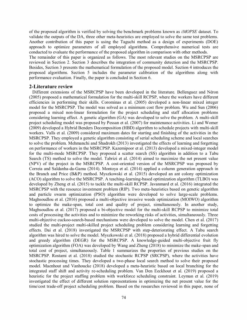
the previous studies investigated the impact of detecting communities of multi-skill workers on the make-span of the project. Moreover, to the best of the authors’ knowledge, none of the previous studies has evaluated the performance of the dandelion algorithm in solving the MSRCPSP.

Table 1. Properties of the previous studies on the MSRCPSP

Research Objective Function Community detection Optimizer Make-span Cost Other Yes No Bellenguez and Néron (2005) * * A heuristic

Corominas et al. (2005) * * * CPLEX Wu and Sun (2006) * * GA Pessan et al. (2007) * * B&B

Li and Womer (2009) * * HBD Valls et al. (2009) * * GA

Mehmanchi and Shadrokh (2013) * * CPLEX Kazemipoor et al. (2013) * * SS, TS

Tabrizi et al. (2014) * * GA Correia and Saldanha-da-Gama (2014) * * CPLEX

Montoya et al. (2014) * * B&P Myszkowski et al. (2015) * * * ACO

Zheng et al. (2015) * * TLBO Javanmard et al. (2016) * * GA, PSO

Maghsoudlou et al. (2016) * * * * MOIWO Maghsoudlou et al. (2017) * * * Cuckoo search

Chen et al. (2017) * * * * NSGA-II Dai et al. (2018) * * * TS

Myszkowski et al. (2018) * * * DEGR Wang and Zheng (2018) * * * FOA

Rostami et al. (2018) * * GA Maenhout and Vanhoucke (2018) * * A mat-heuristic Van Den Eeckhout et al. (2019) * * * * A heuristic

Leyman et al. (2019) * * * * A heuristic This research * * GRA+DA

3-Problem definition 3-1- Community definition A network is represented by an undirected graph denoted as G (V, E), where V and E represent the set of nodes (components of the network) and edges (relations between nodes), respectively. A community is formed by a group of nodes which have more intra-relations than inter-relations. Adjacency matrix can be used to represent a graph. Suppose that 𝐴 = [𝐴𝑖𝑗] denotes the adjacency matrix of the graph G. In the adjacency matrix, if the element in row i and column j equals to 1, there is an edge between nodes i and j in the graph. The degree of node i is calculated as 𝑘𝑖 = ∑ 𝐴𝑖𝑗𝑗 . Let assume that the node i is a member in a sub-graph 𝐿 ⊂ 𝐺. With respect to sub-graph L, the degree of node i is computed as 𝑘𝑖(𝐿) = 𝑘𝑖

𝑖𝑛(𝐿) +

𝑘𝑖𝑜𝑢𝑡(𝐿). 𝑘𝑖

𝑖𝑛(𝐿) is the number of edges connecting other nodes to node i in sub-graph S, while 𝑘𝑖𝑜𝑢𝑡 (𝐿) is

the number of edges connecting node i to the rest of the graph. A sub-graph like L is a strong community if 𝑘𝑖

𝑖𝑛(𝐿) > 𝑘𝑖𝑜𝑢𝑡(𝐿)(∀𝑖 ∈ 𝐿). Detecting communities in complex networks is essentially a clustering

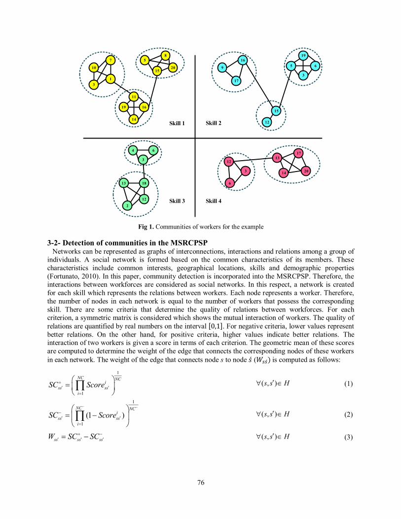
problem (Rahimi et al., 2017). In this paper, the community detection has been applied to the MSRCPSP to detect groups of workforces. Then, it is possible to assign compatible and collaborate teams to the activities that require more than one worker in each day. Therefore, for each skill, a network is formed that shows the relations of the workers that have the corresponding skill. For example, consider a project that needs four skills. Twenty multi-skill workers are available to execute activities of this project. Since this project requires four skills, four networks are formed which show the relations of workers. Figure 1 illustrates these four networks. The edges show the relations between workers. Dashed circles show the identified communities in each network.

76

Skill 4

1

10

7

3

58

2015

11

1619

14

4 6

3

1813

122

9

16

17

15

12

19

65

3

12

3

6

14 20

1713

Skill 3

Skill 1 Skill 2

Fig 1. Communities of workers for the example

3-2- Detection of communities in the MSRCPSP Networks can be represented as graphs of interconnections, interactions and relations among a group of individuals. A social network is formed based on the common characteristics of its members. These characteristics include common interests, geographical locations, skills and demographic properties (Fortunato, 2010). In this paper, community detection is incorporated into the MSRCPSP. Therefore, the interactions between workforces are considered as social networks. In this respect, a network is created for each skill which represents the relations between workers. Each node represents a worker. Therefore, the number of nodes in each network is equal to the number of workers that possess the corresponding skill. There are some criteria that determine the quality of relations between workforces. For each criterion, a symmetric matrix is considered which shows the mutual interaction of workers. The quality of relations are quantified by real numbers on the interval [0,1]. For negative criteria, lower values represent better relations. On the other hand, for positive criteria, higher values indicate better relations. The interaction of two workers is given a score in terms of each criterion. The geometric mean of these scores are computed to determine the weight of the edge that connects the corresponding nodes of these workers in each network. The weight of the edge that connects node s to node �́� (𝑊𝑠�́�) is computed as follows:

1

1

NC NCi

ss ssi

SC Score

( , )s s H (1)

1

1

(1 )NC NC

iss ss

i

SC Score

( , )s s H (2)

ss ss ssW SC SC

( , )s s H (3)

77

Where, 𝑆𝐶𝑠�́�+ and 𝑆𝐶𝑠�́�

− are the scores of interactions between workers s and �́� in terms of positive and negative criteria, respectively. 𝑁𝐶 is the number of positive criteria, while 𝑁𝐶− denote the number of negative criteria. H is the set of multi-skill workers. 𝑆𝑐𝑜𝑟𝑒𝑠�́�

𝑖 is the score of the interaction between workers s and �́�. The weights of the edges are given as parameters for the proposed MSRCPSP model. Table 2 describes the criteria which have been considered to model the relations between workers. For the “Difference in personalities” and “Competition”, lower values indicate better relations, while for the “Previous experiences”, “Trust” and “Mutual respect”, higher values represent stronger relations.

Table 2. The criteria used to model the relations between workers Criterion Description

Difference in personalities

Different personalities of workers can cause workplace conflicts. Workers have different experiences and backgrounds which form their personalities. If the workforces fail to understand each other, issues may arise in the workplaces.

Competition Another cause of conflict in workplaces is unhealthy competition among workforces. Unhealthy competition results in disappointment in teams and promotes individualism.

Previous experiences Good or bad experiences can affect the way the workforces interact with each other. The way they were treated previously can often influence their acting in the future.

Trust Trust plays a remarkable role for having a successful collaboration. The workers in trusting relations allow one another to do their duties without unnecessary monitoring and supervision.

Mutual respect Respectful interactions between workers lead to promising and positive collaboration.

Modularity (Q) is a metric that measures the quality of network partitions. High values of modularity imply that the connections between the nodes within a community are dense, while the connections between the nodes in different communities are sparse. Modularity is a well-known metric, which is usually used in optimization methods to detect community structures of networks. This metric is computed as follows (Fortunato, 2010):

,

.1 ( , )2 2

NNi j

ij i ji j

k kQ A C C

NE NE

(4)

Where, 𝐴𝑖𝑗 is an element in the adjacency matrix (A) that is equal to 1 if the nodes i and j are connected together. Otherwise, 𝐴𝑖𝑗 is equal to 0. NN and NE denote the number of nodes and edges, respectively. 𝑘𝑖 and 𝑘𝑗 are the degrees of the nodes i and j, respectively. 𝐶𝑖 is the community of the node i, while 𝐶𝑗 is the community of the node j. 𝜌(𝐶𝑖 , 𝐶𝑗 ) is equal to 1 if 𝐶𝑖 = 𝐶𝑗 . Modularity can also be used for the weighted graphs. In this respect, 𝑘𝑖 and 𝑘𝑗 are replaced with 𝑠𝑡𝑖 and 𝑠𝑡𝑗 that represent the strengths of the nodes i and j, respectively. Node strength is the sum of weights of the edges that are connected to the node. Total number of edges (NE) in Eq. (4) is replaced with the sum of weights of all edges (SW). 𝑊𝑖𝑗 is the weight of the edge that connects nodes i and j. Modularity can be computed for weighted networks as follows (Fortunato, 2010):

,

.1 ( , )2 2

NNi j

ij i ji j

st stQ W C C

SW SW

(5)

Optimizing modularity helps to find high quality communities of workers for each skill. In the MSRCPSP, some activities may need more than one worker in each day of their durations to perform their required skills. Using effective teams will reduce the project completion time. Having detected communities of workers for each skill, it is possible to choose appropriate workers from identified

78

communities. Therefore, a procedure is proposed to assign workers to the activities that require more than one worker. If activity j requires 𝑁𝑅𝑊𝑗𝑚(𝑁𝑅𝑊𝑗𝑚 > 1) workers with skill m, one of the detected communities in the 𝑚𝑡ℎ network is selected, randomly. Note that the number of nodes in the selected community cannot be less than the number of workers by activity j. Suppose that the community C has been randomly selected and there are NNC nodes in this community (𝑁𝑁𝐶 > 1 and 𝑁𝑁𝐶 ≥ 𝑁𝑅𝑊𝑗𝑚 ). Then, 𝑁𝑅𝑊𝑗𝑚 number of workers are selected randomly from the community C to assign to activity j. Algorithm 1 describes the process of assigning workers to activities.

Algorithm 1: Process of assigning workers to activities Notations:

N The number of project activities (𝑗 = 1, … , 𝑁) M The number of required skills (𝑚 = 1, … , 𝑀)

𝑁𝑅𝑊𝑗𝑚 The number of required workers to perform skill m of activity j 1. For j =1 to N do 2. For m =1 to M do 3. If 𝑁𝑅𝑊𝑗𝑚 > 1 4. Select a random community in the network m;

5. Choose 𝑁𝑅𝑊𝑗𝑚 number of workers from the selected community to perform skill m of activity j;

6. Else 7. Choose a random worker with skill m for activity j; 8. End If 9. End For

10. End For

3-3- Multi-skill resource-constrained project scheduling problem (MSRCPSP) The MSRCPSP involves a project with N interrelated activities which should be scheduled subject to two types of constraints (Chand et al., 2018):

1. Precedence constraints: These constraints represent the interdependence between activities. If activity i is a predecessor of activity j, the activity j cannot be started before activity i is completed.

2. Resource constraints: In the MSRCPSP, these constraints represent limitations on workforces. For each project, there is a set of S multi-skill workers. Each activity may need one or more workers to be executed. The daily resource usage for skill m cannot exceed the number of available workers with this skill. Each worker is only able to perform one activity in each day.

Each activity j needs 𝑑𝑗 time units to be completed. Each worker is able to perform at least one skill from the skill pool (e.g. electrician, machinist, analyst, tester, etc.). For each skill of a worker, there is a certain familiarity level. Each activity requires a predefined number of skills with different standard levels. A worker s is able to perform activity j, if and only if the worker s has the required skill and his/her familiarity level is not less than the standard level (Wang and Zheng, 2018). Workers are allowed to perform at most one activity in each period. The aim of the MSRCPSP is to minimize the make-span of the project. This problem is NP-hard and therefore the exact methods may fail to solve the large-sized problems to optimality in polynomial time (Blazewicz et al., 1983). For large-sized problems, heuristics and meta-heuristics are used to obtain good approximate solutions in a reasonable computation time (Chand et al., 2018). Let G (J, E) be an activity-on-node (AON) network to show the precedence relations between project activities. J represents a set of interrelated and non-preemptive activities and E denotes the set of edges representing Finish-to-Start (FS) precedence relations among activities with zero-time lags. Activities have known durations and they have only one execution mode. The project also includes a

79

dummy start activity 0 and a dummy finish activity N+1, which mark the start time and finish time of the project, respectively. Dummy activities have zero durations and they require no workforces. For example, consider a project consisting of five non-dummy activities to be executed by six workers. This project needs four skills and there are three familiarity levels for each skill. The activities “0” and “6” are dummy

start and finish activities, respectively. Figure 2 depicts the AON network of the project. Nodes and edges represent the project activities and precedence relations, respectively. Nodes are weighted with standard durations.

0

2

2

3

1

3

0

0

1

2

3

4

5

6

Fig 2. The AON network of the example

Table 3 shows the required skills of activities. In table 3, the standard level of each skill and the number of required workers are also reported. Table 4 shows the skills which can be executed by workers. Moreover, table 4 reports the familiarity levels of workers.

Table 3. Required skills and standard levels of activities Activity Skill Standard level Number of required workers

1 1 3 2 3 1 1

2 2 2 2

3 4 1 1 4 2 3 1

5 3 2 2

Table 4. Skills and familiarity levels of workers

Worker Skill Familiarity level

1 1 3 4 3

2 3 2

3 2 3 3 1

4 2 2 3 2 4 2

5 1 3 3 1

6 4 2

80

Based on the information provided in tables 3 and 4, table 5 shows the workers that must be assigned to each activity. According to table 5, the workers “1” and “5” are capable to perform skill “1” of activity “1”. Workers “2”, “3”,”4” and “5” are eligible to execute skill “3” of activity “1”. Workers “3” and “4”

can be assigned to activity “2”. Workers “1”, “4” and “6” are able to execute required skills of activity

“3”. Worker “3” is the only eligible worker to execute activity “4”. Workers “2” and “4” are the qualified workforces to perform the activity “5”. Table 6 shows the workers assigned to activities based on the information given in table 5.

Table 5. Capability of workers for performing required skills of activities

Activity Skill Worker 1 2 3 4 5 6

1 1 × × × × 3 × ×

2 2 × × × × 3 4 × × × 4 2 × × × × × 5 3 × × × ×

Table 6. The workers assigned to activities for the example Activity Skill Assigned worker

1 1 Workers “1” and “5” 3 Worker “4”

2 2 Workers “3” and “4” 3 4 Worker “6” 4 2 Worker “3” 5 3 Workers “2” and “4”

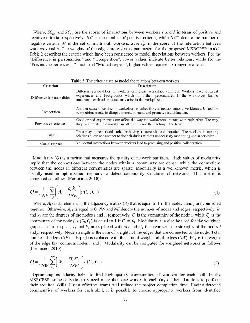
For the project depicted in figure 2, a feasible order of activities to enter scheduling process is [2 1 3 5 4]. Figure 3 shows the Gantt chart associated with the feasible schedule [2 1 3 5 4]. The make-span of the project is equal to 11 time periods which has been obtained with respect to precedence relations and resource limitations.

Fig 3. A feasible schedule for the MSRCPSP

The objective of the proposed model is minimization of project completion time. In the following, section 3.3.1 introduces the notations of sets, parameters and decision variables. Section 3.3.2 presents the mathematical formulation and its description.

81

3-3-1-Notations The following notations are used to formulate the MSRCPSP:

Sets

J Set of project activities ( , 0,..., 1j j N ) Set of required skills ( 1,...,m M ) Set of time periods ( 1,...,t T ) H Set of multi-skill workers ( , 1,...,s s S )

j Set of workers assigned to activity j j Set of predecessors of activity j Parameters

jd Standard duration of activity j

jm The required standard level of skill m for activity j

sm The level that worker s masters skill m

jmNRW The required number of workers to perform skill m of activity j

ssW The weight of the edge that connects node s (worker s) to node �́� (worker �́�) in all networks

sm Equals 1 if worker s has skill m, otherwise it equals 0 jm Equals 1 if activity j requires skill m, otherwise it equals 0 Variables jp Processing time required by the workers assigned to activity j jF Finish time of activity j

js Sum of the weights of the edges that connect worker s (node s) to his/her co-workers in performing activity j

jmAS Average weights of the edges that connect the workers assigned to skill m of activity j Z Make-span of the project

jtU Equals 1 if activity j starts at the beginning of period t, otherwise it equals 0 jsR Equals 1 if worker s is assigned to activity j, otherwise it equals 0

jst Equals 1 if worker s is performing activity j in period t, otherwise it equals 0

ss j Equals 1 if worker s cooperates with worker �́� in performing activity j, otherwise it equals 0 3-3-2-Mathematical formulation

( 1)1

.T

N tt

MinZ t U

(6)

Subject to:

11

Tjt

tU

; j J (7)

.js ss ss jW ; jj J , s s (8)

82

/ (2 )j

jm js jms

AS NRW

; j J , m (9)

max( / )j j jmm

p d AS ; j J (10)

j j jF F p ; jj, j J , j (11)

1

Sjs sm jm jm

sR . .

; j J , m (12)

sm jm ; j J , s H (13) 1

01

Njst

j

; s H, t (14)

0j j js jmp ,F , ,AS ,Z ; j J , s H , m (15)

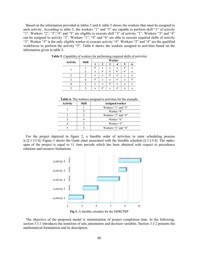
0 1jt js jst ss jU ,R , , , ; j J , s H , m , t (16) The objective function (6) is the minimization of the project completion time. Constraint (7) guarantees that each activity starts exactly once. Equation (8) computes the sum of the weights of the edges that connect worker s to his/her co-workers in performing activity j. Equation (9) calculates the average weights of the edges that connect the workers assigned to skill m of activity j. Equation (10) determines the processing time required by the workers assigned to activity j. Constraint (11) represents the precedence relations between activities. Constraints (12) and (13) secure that each activity can only be performed by the capable workers. Constraint (14) guarantees that each worker can only perform one activity in each period. Constraints (15) and (16) define the feasible scope of decision variables.

3-3-3-Managerial insights The proposed model in this paper can be used in various projects, where multi-skill workers are available as resources. For instance, this model can utilized for scheduling activities of software development projects. Information technology (IT) enterprises have a limited number of employees with different skills. Each employee masters various computer languages. Due to scarcity of multi-skill personnel, the problem of scheduling activities in software development projects can be considered as a multi-skill resource-constrained project scheduling problem.

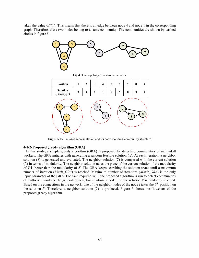
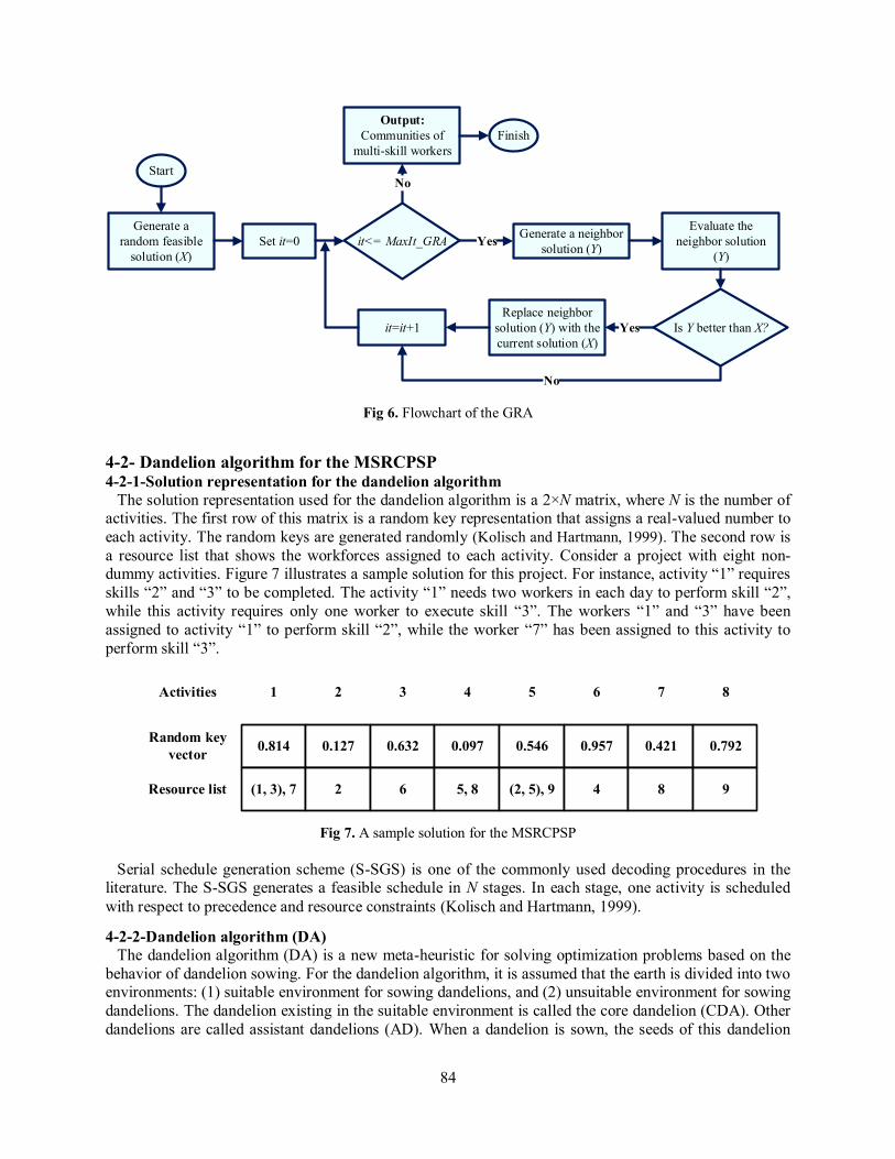
4-Solution approaches 4-1- Greedy algorithm for detecting communities of workers 4-1-1-Solution representation for the greedy algorithm In this study, the locus-based adjacency representation (LAR) (Handl and Knowles, 2007) has been used as the representation scheme of the proposed greedy algorithm. In this graph-based representation, each solution is an array of N genes. Each gene represents a node in the graph and it is connected randomly to one of its neighbors. Each solution is decoded as a graph in which the value of j assigned to the gene i is interpreted as a link between node i and node j. Connected nodes of each solution are considered as communities. By using this scheme, the number of communities is determined during the decoding procedure. Therefore, the algorithm does not require to know the number of communities in advance. This decoding procedure can be carried out in a linear time (Shi et al., 2010). Figure 4 illustrates an example of the LAR scheme for a network with nine nodes. A feasible solution and the interpretation of this solution are depicted in figure 5. As shown in figure 5, each gene of this solution has taken a value in the range of 1 to 9. According to figure 5, for instance, the fourth node has

83

taken the value of “1”. This means that there is an edge between node 4 and node 1 in the corresponding graph. Therefore, these two nodes belong to a same community. The communities are shown by dashed circles in figure 5.

1 3 5

2

7

986

4

Fig 4. The topology of a sample network

1 3 5

2

7

986

4

Position

Solution (Genotype)

1 2 3 4 5 6 7 8 9

3 4 1 6 51 8 9 7

Fig 5. A locus-based representation and its corresponding community structure

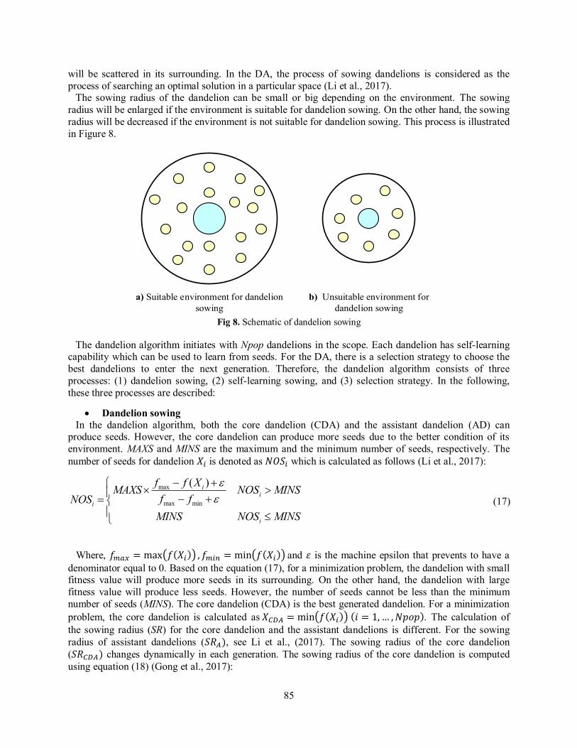
4-1-2-Proposed greedy algorithm (GRA) In this study, a simple greedy algorithm (GRA) is proposed for detecting communities of multi-skill workers. The GRA initiates with generating a random feasible solution (X). At each iteration, a neighbor solution (Y) is generated and evaluated. The neighbor solution (Y) is compared with the current solution (X) in terms of modularity. The neighbor solution takes the place of the current solution if the modularity of Y is better than the modularity of X. The GRA keeps searching the solution space until a maximum number of iteration (MaxIt_GRA) is reached. Maximum number of iterations (MaxIt_GRA) is the only input parameter of the GRA. For each required skill, the proposed algorithm is run to detect communities of multi-skill workers. To generate a neighbor solution, a node i on the solution X is randomly selected. Based on the connections in the network, one of the neighbor nodes of the node i takes the 𝑖𝑡ℎ position on the solution X. Therefore, a neighbor solution (Y) is produced. Figure 6 shows the flowchart of the proposed greedy algorithm.

84

Start

Set it=0 it<= MaxIt_GRA Generate a neighbor solution (Y)

Evaluate the neighbor solution

(Y)

Is Y better than X?Replace neighbor

solution (Y) with the current solution (X)

it=it+1

Yes

Yes

No

Output: Communities of

multi-skill workersFinish

No

Generate a random feasible

solution (X)

Fig 6. Flowchart of the GRA

4-2- Dandelion algorithm for the MSRCPSP 4-2-1-Solution representation for the dandelion algorithm The solution representation used for the dandelion algorithm is a 2×N matrix, where N is the number of activities. The first row of this matrix is a random key representation that assigns a real-valued number to each activity. The random keys are generated randomly (Kolisch and Hartmann, 1999). The second row is a resource list that shows the workforces assigned to each activity. Consider a project with eight non-dummy activities. Figure 7 illustrates a sample solution for this project. For instance, activity “1” requires

skills “2” and “3” to be completed. The activity “1” needs two workers in each day to perform skill “2”, while this activity requires only one worker to execute skill “3”. The workers “1” and “3” have been assigned to activity “1” to perform skill “2”, while the worker “7” has been assigned to this activity to perform skill “3”.

0.814 0.127 0.632 0.097 0.546 0.957 0.421 0.792

(1, 3), 7 2 6 5, 8 (2, 5), 9 4 8 9

Random key vector

Resource list

1 2 3 4 5 6 7 8Activities

Fig 7. A sample solution for the MSRCPSP

Serial schedule generation scheme (S-SGS) is one of the commonly used decoding procedures in the literature. The S-SGS generates a feasible schedule in N stages. In each stage, one activity is scheduled with respect to precedence and resource constraints (Kolisch and Hartmann, 1999).

4-2-2-Dandelion algorithm (DA) The dandelion algorithm (DA) is a new meta-heuristic for solving optimization problems based on the behavior of dandelion sowing. For the dandelion algorithm, it is assumed that the earth is divided into two environments: (1) suitable environment for sowing dandelions, and (2) unsuitable environment for sowing dandelions. The dandelion existing in the suitable environment is called the core dandelion (CDA). Other dandelions are called assistant dandelions (AD). When a dandelion is sown, the seeds of this dandelion

85

will be scattered in its surrounding. In the DA, the process of sowing dandelions is considered as the process of searching an optimal solution in a particular space (Li et al., 2017). The sowing radius of the dandelion can be small or big depending on the environment. The sowing radius will be enlarged if the environment is suitable for dandelion sowing. On the other hand, the sowing radius will be decreased if the environment is not suitable for dandelion sowing. This process is illustrated in Figure 8.

a) Suitable environment for dandelion sowing

b) Unsuitable environment for dandelion sowing

Fig 8. Schematic of dandelion sowing

The dandelion algorithm initiates with Npop dandelions in the scope. Each dandelion has self-learning capability which can be used to learn from seeds. For the DA, there is a selection strategy to choose the best dandelions to enter the next generation. Therefore, the dandelion algorithm consists of three processes: (1) dandelion sowing, (2) self-learning sowing, and (3) selection strategy. In the following, these three processes are described:

Dandelion sowing In the dandelion algorithm, both the core dandelion (CDA) and the assistant dandelion (AD) can produce seeds. However, the core dandelion can produce more seeds due to the better condition of its environment. MAXS and MINS are the maximum and the minimum number of seeds, respectively. The number of seeds for dandelion 𝑋𝑖 is denoted as 𝑁𝑂𝑆𝑖 which is calculated as follows (Li et al., 2017):

max

max min

( )ii

i

i

f f XMAXS NOS MINSf fNOS

MINS NOS MINS

(17)

Where, 𝑓𝑚𝑎𝑥 = max(𝑓(𝑋𝑖)) , 𝑓𝑚𝑖𝑛 = min(𝑓(𝑋𝑖)) and 𝜀 is the machine epsilon that prevents to have a denominator equal to 0. Based on the equation (17), for a minimization problem, the dandelion with small fitness value will produce more seeds in its surrounding. On the other hand, the dandelion with large fitness value will produce less seeds. However, the number of seeds cannot be less than the minimum number of seeds (MINS). The core dandelion (CDA) is the best generated dandelion. For a minimization problem, the core dandelion is calculated as 𝑋𝐶𝐷𝐴 = min(𝑓(𝑋𝑖)) (𝑖 = 1, … , 𝑁𝑝𝑜𝑝). The calculation of the sowing radius (SR) for the core dandelion and the assistant dandelions is different. For the sowing radius of assistant dandelions (𝑆𝑅𝐴), see Li et al., (2017). The sowing radius of the core dandelion (𝑆𝑅𝐶𝐷𝐴) changes dynamically in each generation. The sowing radius of the core dandelion is computed using equation (18) (Gong et al., 2017):

86

1( ) ( 1) 1

( 1) 1CDA CDA

CDA

UB LB tSR t SR t r g

SR t e g

(18)

Where, LB and UB denote the lower and upper bounds of the search space, respectively. 𝑆𝑅𝐶𝐷𝐴(𝑡) is the sowing radius of the core dandelion in generation t. At the initial step, the sowing radius of the CDA is set to the diameter of the search space. In the above equation, r and e represent the withering and growth factors, respectively. 𝑔 stands for the growth trend, which can be computed by equation (19) (Gong et al., 2017):

( )( 1)

CDA

CDA

f tgf t

(19)

Where, 𝜀 is the machine epsilon that prevents to have a denominator equal to 0. When 𝑔 = 1, it implies that the DA has not found a better solution in this generation than the previous generation. Therefore, it is more likely to find a better solution by reducing the sowing radius. The withering factor (r) is used to describe this situation. The value of r should be in [0.9, 1). On the other hand, if 𝑔 ≠ 1, the DA has obtained a better solution in this generation than the previous generation. In this case, the place is appropriate for sowing, and the algorithm should sow in a wider range. Increasing the sowing radius significantly speeds up the convergence rate. When 𝑔 ≠ 1, the growth factor e is used and its value should be in (1, 1.1] (Gong et al., 2017). If 𝑋𝑖 is a core dandelion, its seeds are calculated as 𝑋𝑖 = 𝑋𝑖 +𝑟𝑎𝑛𝑑(0, 𝑆𝑅𝐶𝐷𝐴). If 𝑋𝑖 is an assistant dandelion, we use 𝑋𝑖 = 𝑋𝑖 + 𝑟𝑎𝑛𝑑(0, 𝑆𝑅𝐴) to obtain its seeds (Li et al., 2017).

Self-learning sowing Dandelions have self-learning ability which enables them to find the better direction to the optimal solution. By self-learning ability, each dandelion can use information from the seeds produced by the core dandelion. This procedure is called the self-learning sowing which helps the DA not to get stuck in the local optima. Besides, this procedure maintains the diversity of the population. The self-learning sowing is designed as follows (Li et al., 2017):

( )CDA CDA CDAX X X (20) Where, 𝑋𝐶𝐷𝐴 is the core dandelion, while �́�𝐶𝐷𝐴 is the new core dandelion obtained by using the seeds. 𝛼 is the set of seeds and 𝜇𝛼 is the average value of seeds. The self-learning sowing procedure is run for a predefined number of iterations.

Selection strategy The DA keeps the best dandelions for the next iterations. Therefore, after completion of each iteration, the best dandelions in terms of fitness value are preserved.

Framework of the DA Figure 9 illustrates the framework of the DA. NOS and NSLD denote the total number of normal seeds and the number of self-learning seeds, respectively. In this respect, (1 + 𝑁𝑂𝑆 + 𝑁𝑆𝐿𝐷) number of seeds are evaluated in each iteration. Suppose that the stopping criterion of the DA is the maximum number of iterations (MaxIt). Therefore, the complexity of the DA is 𝑂(𝑀𝑎𝑥𝐼𝑡 × (1 + 𝑁𝑂𝑆 + 𝑁𝑆𝐿𝐷)) (Li et al., 2017).

87

StartGenerate Npop

random dandelions

Each dandelion produce its own

seeds

Determine the locations of the produced seeds

Evaluate the seeds

it <= MaxItSelect the best Npop dandelions

Finish

Yes

No

Set it =1

it = it + 1

Fig 9. Framework of the DA

5-Computational experiments In this section, the algorithms are tuned by means of the Taguchi method. The results of the GRA for detecting communities of workers are reported. Test problems of the MSRCPSP and the performance measures of algorithms are introduced. The results of the DA are compared with the genetic algorithm (GA) (Hartmann, 1998), harmony search (HS) (Giran et al., 2017) and differential evolution (DE) (Afshar-Nadjafi et al., 2015). The GRA, DA, GA, HS, DE are coded in the MATLAB software (R2017a) that runs on a personal computer with Intel Core 2 Quad processor Q8200 (4M Cache, 2.33 GHz, 1333 MHz FSB) and 4GB memory.

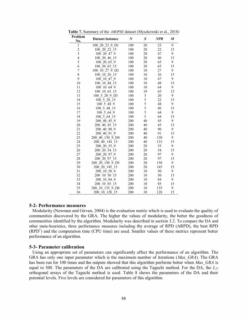
5-1- Test problems In this study, the iMOPSE dataset proposed by Myszkowski et al. (2018) is used to evaluate the performance of the algorithms. The iMOPSE dataset has been artificially generated based on real-world projects, which is available at http://imopse.ii.pwr.wroc.pl/. The characteristics of test problems include the number of project activities (N), the number of available workers (S), the number of precedence relations between activities (NPR), and the number of required skills (M). Table 7 shows the properties of the iMOPSE dataset. Test problems with 100 activities are considered as small size problems, while test problems with 200 activities are considered as large size problems. In the iMOPSE dataset, each worker is able to perform six different skills.

88

Table 7. Summary of the iMOPSE dataset (Myszkowski et al., 2018) Problem

No. Dataset instance N S NPR M

1 100_20_23_9_D1 100 20 23 9 2 100_20_22_15 100 20 22 15 3 100_20_47_9 100 20 47 9 4 100_20_46_15 100 20 46 15 5 100_20_65_9 100 20 65 9 6 100_20_65_15 100 20 65 15 7 100_10_27_9_D2 100 10 27 9 8 100_10_26_15 100 10 26 15 9 100_10_47_9 100 10 47 9 10 100_10_48_15 100 10 48 15 11 100_10_64_9 100 10 64 9 12 100_10_65_15 100 10 65 15 13 100_5_20_9_D3 100 5 20 9 14 100_5_20_15 100 5 22 15 15 100_5_48_9 100 5 48 9 16 100_5_48_15 100 5 46 15 17 100_5_64_9 100 5 64 9 18 100_5_64_15 100 5 64 15 19 200_40_45_9 200 40 45 9 20 200_40_45_15 200 40 45 15 21 200_40_90_9 200 40 90 9 22 200_40_91_9 200 40 91 15 23 200_40_130_9_D4 200 40 130 9 24 200_40_144_15 200 40 133 15 25 200_20_55_9 200 20 55 9 26 200_20_54_15 200 20 54 15 27 200_20_97_9 200 20 97 9 28 200_20_97_15 200 20 97 15 29 200_20_150_9_D5 200 20 150 9 30 200_20_145_15 200 20 145 15 31 200_10_50_9 200 10 50 9 32 200_10_50_15 200 10 50 15 33 200_10_84_9 200 10 84 9 34 200_10_85_15 200 10 85 15 35 200_10_135_9_D6 200 10 135 9 36 200_10_128_15 200 10 128 15

5-2- Performance measures Modularity (Newman and Girvan, 2004) is the evaluation metric which is used to evaluate the quality of communities discovered by the GRA. The higher the values of modularity, the better the goodness of communities identified by the algorithm. Modularity was described in section 3.2. To compare the DA and other meta-heuristics, three performance measures including the average of RPD (ARPD), the best RPD (RPD*) and the computation time (CPU time) are used. Smaller values of these metrics represent better performance of an algorithm. 5-3- Parameter calibration Using an appropriate set of parameters can significantly affect the performance of an algorithm. The GRA has only one input parameter which is the maximum number of iterations (Max_GRA). The GRA has been run for 100 times and the outputs showed that this algorithm performs better when Max_GRA is equal to 300. The parameters of the DA are calibrated using the Taguchi method. For the DA, the L25 orthogonal arrays of the Taguchi method is used. Table 8 shows the parameters of the DA and their potential levels. Five levels are considered for parameters of this algorithm.

89

Table 8. Parameters and their levels for the DA Parameter Levels

Symbols Parameters Level 5

Level 4

Level 3

Level 2

Level 1

0.98 0.96 0.94 0.92 0.90 r Withering factor 1.09 1.07 1.05 1.03 1.01 e Growth factor

5 4 3 2 1 NSLD The number of self-learning dandelions 300 200 100 50 20 Npop Population size 500 300 200 100 50 MaxIt Maximum number of iterations

Taguchi categorized objective functions into three groups: (1) “Smaller is better”, (2) “Larger is better”,

and (3) “Nominal is better”. Most of the objective functions in the project scheduling problem are

grouped as “Smaller is better” type (Afruzi et al., 2014). The Signal-to-Noise (S/N) ratio of the “Smaller is better” type is calculated as follows (Mousavi et al., 2016):

210/ 10 ( )S N Log OFV (21)

Where, OFV is the objective function value which is defined as the project completion time. The goal is to find the parameter values that maximize the S/N ratio. Five large size problems with 200 activities are chosen randomly from the iMOPSE dataset to conduct the Taguchi method. Each problem is run for ten times to remove uncertainties. Therefore, 50 outputs will be obtained for each experiment. The best output among 10 runs is considered as the result of each problem. The make-span of the project for each experiment is transformed into the relative percentage difference (RPD). The RPD is calculated using equation (22) (Gao et al., 2013):

*

* 100; 0 100SolMethod SolRPD RPDSol

(22)

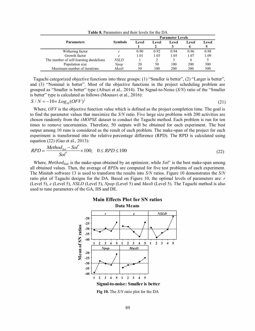
Where, 𝑀𝑒𝑡ℎ𝑜𝑑𝑆𝑜𝑙 is the make-span obtained by an optimizer, while 𝑆𝑜𝑙∗ is the best make-span among all obtained values. Then, the average of RPDs are computed for five test problems of each experiment. The Minitab software 13 is used to transform the results into S/N ratios. Figure 10 demonstrates the S/N ratio plot of Taguchi designs for the DA. Based on Figure 10, the optimal levels of parameters are: r (Level 5), e (Level 5), NSLD (Level 5), Npop (Level 5) and MaxIt (Level 5). The Taguchi method is also used to tune parameters of the GA, HS and DE.

54321

-20-25-30-35-40

54321 54321

54321

-20-25-30-35-40

54321

r

Mea

n of

SN

ratio

s

e NSLD

Npop MaxIt

Main Effects Plot for SN ratiosData Means

Signal-to-noise: Smaller is better

Fig 10. The S/N ratio plot for the DA

90

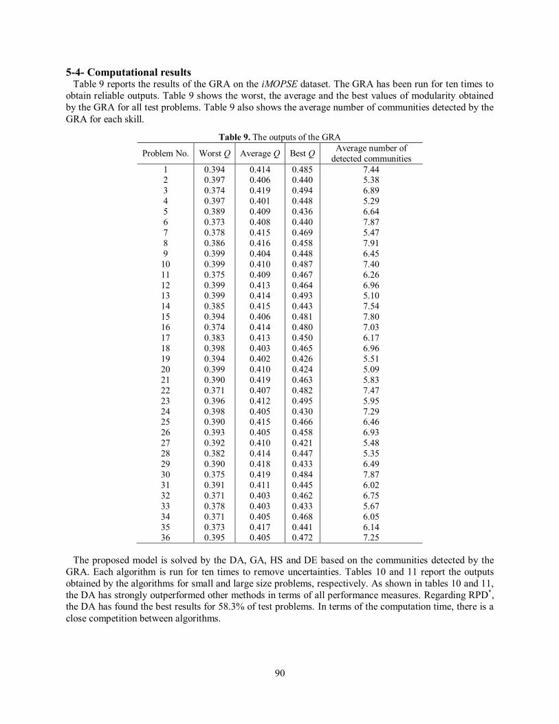
5-4- Computational results Table 9 reports the results of the GRA on the iMOPSE dataset. The GRA has been run for ten times to obtain reliable outputs. Table 9 shows the worst, the average and the best values of modularity obtained by the GRA for all test problems. Table 9 also shows the average number of communities detected by the GRA for each skill.

Table 9. The outputs of the GRA

Problem No. Worst Q Average Q Best Q Average number of detected communities

1 0.394 0.414 0.485 7.44 2 0.397 0.406 0.440 5.38 3 0.374 0.419 0.494 6.89 4 0.397 0.401 0.448 5.29 5 0.389 0.409 0.436 6.64 6 0.373 0.408 0.440 7.87 7 0.378 0.415 0.469 5.47 8 0.386 0.416 0.458 7.91 9 0.399 0.404 0.448 6.45

10 0.399 0.410 0.487 7.40 11 0.375 0.409 0.467 6.26 12 0.399 0.413 0.464 6.96 13 0.399 0.414 0.493 5.10 14 0.385 0.415 0.443 7.54 15 0.394 0.406 0.481 7.80 16 0.374 0.414 0.480 7.03 17 0.383 0.413 0.450 6.17 18 0.398 0.403 0.465 6.96 19 0.394 0.402 0.426 5.51 20 0.399 0.410 0.424 5.09 21 0.390 0.419 0.463 5.83 22 0.371 0.407 0.482 7.47 23 0.396 0.412 0.495 5.95 24 0.398 0.405 0.430 7.29 25 0.390 0.415 0.466 6.46 26 0.393 0.405 0.458 6.93 27 0.392 0.410 0.421 5.48 28 0.382 0.414 0.447 5.35 29 0.390 0.418 0.433 6.49 30 0.375 0.419 0.484 7.87 31 0.391 0.411 0.445 6.02 32 0.371 0.403 0.462 6.75 33 0.378 0.403 0.433 5.67 34 0.371 0.405 0.468 6.05 35 0.373 0.417 0.441 6.14 36 0.395 0.405 0.472 7.25

The proposed model is solved by the DA, GA, HS and DE based on the communities detected by the GRA. Each algorithm is run for ten times to remove uncertainties. Tables 10 and 11 report the outputs obtained by the algorithms for small and large size problems, respectively. As shown in tables 10 and 11, the DA has strongly outperformed other methods in terms of all performance measures. Regarding RPD*, the DA has found the best results for 58.3% of test problems. In terms of the computation time, there is a close competition between algorithms.

91

Table 10. Comparison of algorithms for small-size problems

Prob. ARPD RPD* Computation time DA GA HS DE DA GA HS DE DA GA HS DE

1 0.38 8.47 5.60 9.07 0.00 8.25 5.54 8.94 38.45 45.68 44.86 45.92 2 0.27 6.59 7.49 6.22 0.00 6.39 7.19 6.09 37.27 43.77 42.45 46.52 3 2.65 9.75 9.80 9.65 2.56 9.45 9.44 9.54 43.22 49.66 50.26 48.62 4 3.90 5.17 6.70 6.75 3.88 5.11 6.55 6.59 39.15 46.86 44.28 44.67 5 4.67 7.19 7.93 5.98 4.12 6.98 7.68 5.94 45.70 52.53 50.91 51.87 6 0.65 6.91 6.12 6.26 0.00 6.78 5.72 6.25 40.12 46.97 46.68 47.61 7 2.84 8.83 8.76 8.08 2.21 8.37 8.39 7.84 55.23 62.81 60.52 62.64 8 2.35 8.98 6.28 7.37 0.00 8.69 6.16 7.14 62.14 69.55 69.59 67.32 9 0.06 5.93 7.53 6.76 0.00 5.45 7.26 6.50 74.21 85.94 81.66 80.41

10 1.69 7.45 8.50 9.15 0.00 7.33 8.26 8.84 78.44 83.99 87.61 85.02 11 0.81 7.23 9.45 7.93 0.00 6.89 9.25 7.75 96.50 102.22 101.95 105.75 12 3.97 8.23 9.80 7.75 3.88 7.74 9.78 7.31 67.56 75.22 74.54 71.89 13 1.56 8.55 7.74 9.59 0.00 8.09 7.34 9.54 149.22 154.30 155.77 156.10 14 2.64 8.77 5.69 6.43 0.00 8.64 5.52 6.09 137.52 143.99 145.44 143.39 15 0.83 6.38 5.75 8.79 0.00 6.31 5.39 8.74 155.06 159.56 167.00 161.35 16 3.01 8.40 6.29 8.77 2.85 8.07 6.04 8.38 165.09 177.02 172.49 170.13 17 1.31 8.28 9.20 6.90 0.00 7.92 8.75 6.45 104.14 116.28 110.50 112.09 18 3.27 5.81 6.27 7.84 3.10 5.64 5.92 7.74 116.24 127.74 123.61 121.74

Avg. 2.05 7.61 7.49 7.74 1.26 7.34 7.23 7.54 83.62 91.34 90.56 90.17

Table 11. Comparison of algorithms for large-size problems

Prob. ARPD RPD* Computation time DA GA HS DE DA GA HS DE DA GA HS DE

19 3.47 3.83 8.70 3.53 3.03 3.29 8.13 3.10 111.58 116.32 117.67 114.71 20 1.59 6.49 4.70 3.38 0.00 6.25 4.39 2.72 93.21 96.69 99.18 94.06 21 4.75 9.72 9.50 6.72 3.67 9.44 8.89 6.25 83.10 88.82 91.32 86.24 22 0.17 5.38 5.45 8.45 0.00 4.68 5.21 8.03 84.70 87.64 82.59 88.88 23 2.19 7.10 4.38 9.54 0.00 6.85 3.70 9.34 81.08 86.51 87.14 84.64 24 1.91 4.57 4.76 3.91 0.00 3.98 4.15 3.28 86.07 88.99 90.73 92.69 25 3.83 8.26 7.31 6.98 2.97 8.02 6.91 6.65 143.35 147.19 147.10 145.50 26 3.98 4.79 6.31 6.29 3.02 4.19 5.89 5.63 224.51 229.64 231.21 227.43 27 0.93 6.54 5.46 3.08 0.00 6.25 5.13 2.81 137.37 143.27 143.75 141.89 28 2.45 7.89 8.82 5.36 0.00 7.62 8.19 4.87 164.68 167.09 169.43 171.58 29 2.23 9.24 7.10 4.14 0.00 8.77 6.83 3.51 223.47 230.12 228.58 227.66 30 3.23 9.72 6.85 8.56 2.47 9.21 6.47 8.10 207.46 213.34 212.40 210.02 31 3.55 6.83 9.42 5.18 3.19 6.43 9.18 4.86 256.61 261.04 259.65 259.90 32 3.77 3.97 5.00 6.70 3.22 3.71 4.71 6.38 247.17 255.35 250.68 251.21 33 1.38 4.05 8.30 4.16 0.00 3.64 8.08 3.51 199.60 209.83 206.95 204.57 34 3.40 4.80 8.28 7.21 2.62 4.13 7.83 6.77 176.83 180.36 179.98 180.14 35 3.28 8.89 5.66 4.84 0.00 8.52 5.01 4.46 344.43 348.97 350.65 349.44 36 0.81 4.78 6.97 7.58 0.00 4.52 6.38 7.19 325.49 330.04 328.46 331.05

Avg. 2.61 6.49 6.83 5.87 1.34 6.08 6.39 5.41 177.26 182.29 182.08 181.20

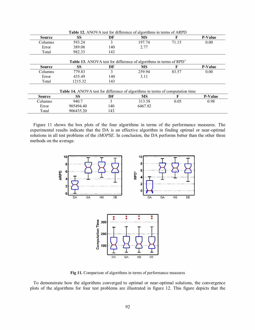
To compare the performances of the algorithms statistically, a one-way analysis of variances at a 95% confidence interval is conducted. Tables 12, 13 and 14 report the ANOVA of algorithms in terms of the ARPD, RPD* and computation time. Based on the results reported in these tables, there is a significant difference between the performances of the algorithms in terms of the ARPD and RPD* metrics, while there is no significant difference between the performances of the algorithms in terms of computation time.

92

Table 12. ANOVA test for difference of algorithms in terms of ARPD Source SS DF MS F P-Value

Columns 593.24 3 197.74 71.15 0.00 Error 389.08 140 2.77 Total 982.33 143

Table 13. ANOVA test for difference of algorithms in terms of RPD*

Source SS DF MS F P-Value Columns 779.83 3 259.94 83.57 0.00

Error 435.49 140 3.11 Total 1215.32 143

Table 14. ANOVA test for difference of algorithms in terms of computation time Source SS DF MS F P-Value

Columns 940.7 3 313.58 0.05 0.98 Error 905494.40 140 6467.82 Total 906435.20 143

Figure 11 shows the box plots of the four algorithms in terms of the performance measures. The experimental results indicate that the DA is an effective algorithm in finding optimal or near-optimal solutions in all test problems of the iMOPSE. In conclusion, the DA performs better than the other three methods on the average.

Fig 11. Comparison of algorithms in terms of performance measures

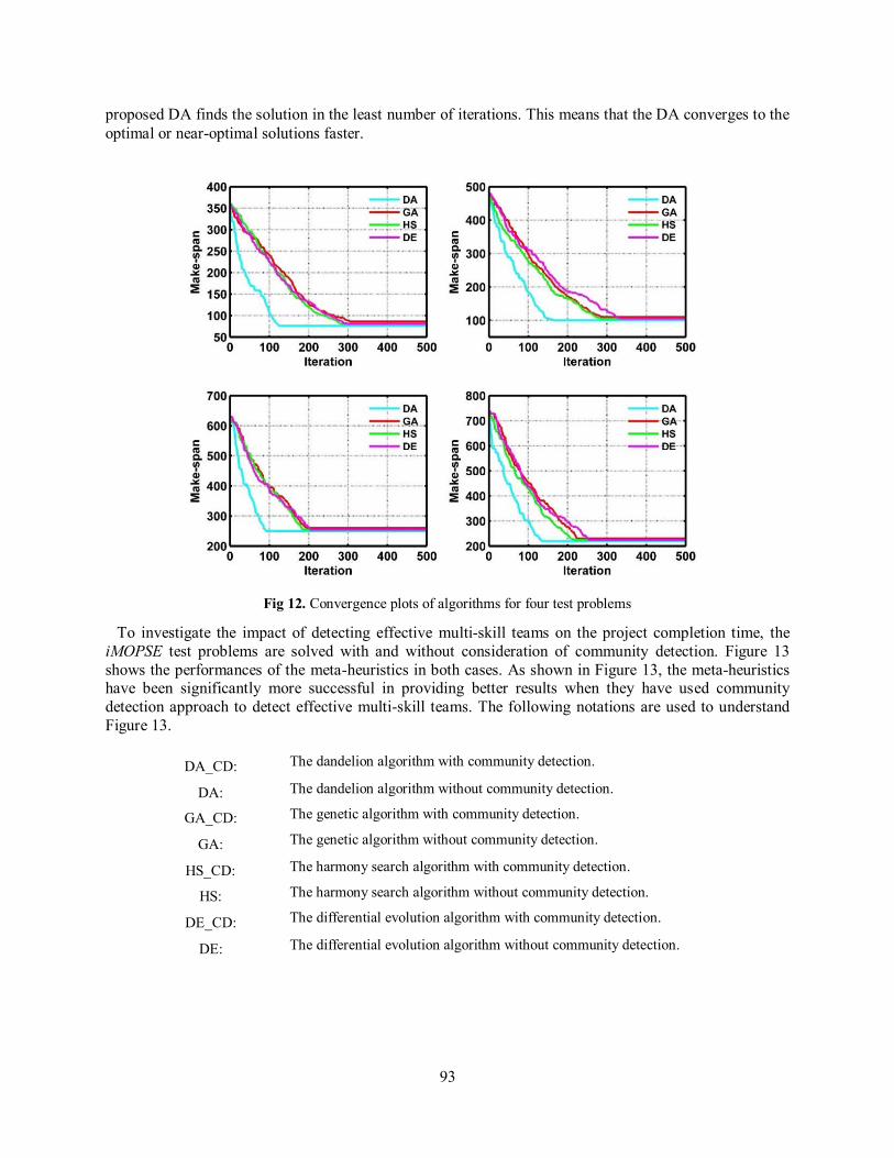
To demonstrate how the algorithms converged to optimal or near-optimal solutions, the convergence plots of the algorithms for four test problems are illustrated in figure 12. This figure depicts that the

93

proposed DA finds the solution in the least number of iterations. This means that the DA converges to the optimal or near-optimal solutions faster.

Fig 12. Convergence plots of algorithms for four test problems

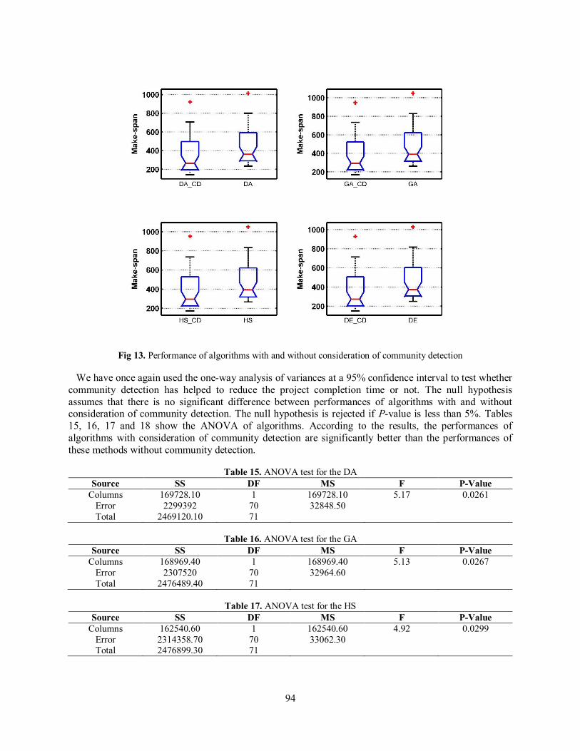
To investigate the impact of detecting effective multi-skill teams on the project completion time, the iMOPSE test problems are solved with and without consideration of community detection. Figure 13 shows the performances of the meta-heuristics in both cases. As shown in Figure 13, the meta-heuristics have been significantly more successful in providing better results when they have used community detection approach to detect effective multi-skill teams. The following notations are used to understand Figure 13.

DA_CD: The dandelion algorithm with community detection.

DA: The dandelion algorithm without community detection.

GA_CD: The genetic algorithm with community detection.

GA: The genetic algorithm without community detection.

HS_CD: The harmony search algorithm with community detection.

HS: The harmony search algorithm without community detection.

DE_CD: The differential evolution algorithm with community detection.

DE: The differential evolution algorithm without community detection.

94

Fig 13. Performance of algorithms with and without consideration of community detection

We have once again used the one-way analysis of variances at a 95% confidence interval to test whether community detection has helped to reduce the project completion time or not. The null hypothesis assumes that there is no significant difference between performances of algorithms with and without consideration of community detection. The null hypothesis is rejected if P-value is less than 5%. Tables 15, 16, 17 and 18 show the ANOVA of algorithms. According to the results, the performances of algorithms with consideration of community detection are significantly better than the performances of these methods without community detection.

Table 15. ANOVA test for the DA Source SS DF MS F P-Value

Columns 169728.10 1 169728.10 5.17 0.0261 Error 2299392 70 32848.50 Total 2469120.10 71

Table 16. ANOVA test for the GA

Source SS DF MS F P-Value Columns 168969.40 1 168969.40 5.13 0.0267

Error 2307520 70 32964.60 Total 2476489.40 71

Table 17. ANOVA test for the HS

Source SS DF MS F P-Value Columns 162540.60 1 162540.60 4.92 0.0299

Error 2314358.70 70 33062.30 Total 2476899.30 71

95

Table 18. ANOVA test for the HS Source SS DF MS F P-Value

Columns 177013.80 1 177013.80 5.39 0.0231 Error 2297127.10 70 32816.10 Total 2474140.90 71

5-5- Findings of computational experiments The novel findings of the computational experiments conducted in this study are listed as follows:

1. In terms of the ARPD metric, the DA has outperformed other algorithms for both small and large size problems. 2. The DA has been more successful than other algorithms in terms of the RPD* and it has achieved the best results for 58.3% of test problems. 3. Based on the results of ANOVA, the performances of algorithms are significantly different in terms of ARPD and RPD*. On the other side, there is no significant difference between algorithms in terms of the computation time. 4. The DA converges to optimal or near-optimal solutions in far less number of iterations comparing to other methods. 5. The results showed that detecting effective teams has a significant impact on reducing the make-span of the project.

6-Conclusion and recommendations for further researches In this paper, the multi-skill resource-constrained project scheduling problem with the goal of minimizing project completion time was considered. The relations between available workers of projects have been modeled as networks. In this respect, for each skill, there is a network that shows the relations between human resources. The weights of the edges in these networks were obtained based on various criteria describing relations between co-workers. Community detection was used to detect the most effective and compatible teams for the activities that require more than one worker in each day. To find high quality communities of multi-skill workers, a greedy algorithm was developed to optimize modularity as a well-known objective in detecting community structure. Having detected communities of workers for each skill, the MSRCPSP was formulated. Due to the NP-hard essence of the MSRCPSP, a dandelion algorithm (DA) with calibrated parameters was developed to solve the problem. The DA was used to solve test problems of the iMOPSE dataset. To evaluate the performance of the DA and to validate the outputs of this method, the solutions were compared to the ones obtained by three other meta-heuristics. The results show the superiority of the proposed dandelion algorithm in terms of most of the performance measures. A one-way analysis of variances was conducted to determine whether the performances of algorithms are significantly different or not. The outputs show that the performances of algorithms are significantly different in terms of ARPD and RPD*, while their performances are not significantly different in terms of computation time. Using effective teams will impose more costs on the project. The impact of using more efficient workers on the cost of project can be studied as a future research opportunity. As another recommendation, other criteria can be taken into account to model the interactions between workers.

96

References Afruzi, E., Najafi, A.A., Roghanian, E., & Mazinani, M. (2014). A Multi-Objective Imperialist Competitive Algorithm for solving discrete time, cost and quality trade-off problems with mode-identity and resource-constrained situations. Computers & Operations Research, 50, 80-96. Afshar-Nadjafi, B., Karimi, H., Rahimi, A., & Khalili, S. (2015). Project scheduling with limited resources using an efficient differential evolution algorithm. Journal of King Saud University, 27(2), 176-184. Bellenguez, O., & Néron, E. (2005). Lower Bounds for the Multi-skill Project Scheduling Problem with Hierarchical Levels of Skills. Practice and Theory of Automated Timetabling V, 3616, 229-243. Blazewicz, J., Lenstra, J.K. & Kan, A. (1983). Scheduling subject to resource constraints: Classification and complexity. Discrete Applied Mathematics, 5, 11-24. Brandes, U., Delling, D., & Gaetler, M. (2008). On Modularity Clustering. Transactions on Knowledge and Data Engineering, 20(2), 172-188. Chand, S., Huynh, Q., Singh, H., Ray, T., & Wagner, M. (2018). On the use of genetic programming to evolve priority rules for resource constrained project scheduling problems. Information Sciences, 432, 146-163. Chen, M., Kuzmin, K., Boleslaw, K., & Szymanski, F. (2014). Community Detection via Maximization of Modularity and Its Variants. IEEE Transactions on Computational Social Systems, 1(1), 46-65. Chen, R., Liang, C., Gu, D., & Leung, J. (2017). A multi-objective model for multi-project scheduling and multi-skilled staff assignment for IT product development considering competency evolution. International Journal of Production Research, 55(21), 6207-6234. Cordeau, J., Laporte, G., Pasin, F., & Ropke, S. (2010). Scheduling technicians and tasks in a telecommunications company. Journal of Scheduling, 13(4), 393-409. Corominas, A., Ojeda, J., & Pastor, R. (2005). Multi-objective allocation of multi-function workers with lower bounded capacity. Journal of the Operational Research Society, 56, 738-743. Correia, I., & Saldanha-da-Gama, F. (2014). The impact of fixed and variable costs in a multi-skill project scheduling problem: An empirical study. Computers & Industrial Engineering, 72, 230-238. Dai, H., Cheng, W., & Guo, P. (2018). An Improved Tabu Search for Multi-skill Resource-Constrained Project Scheduling Problems under Step-Deterioration. Arabian Journal for Science and Engineering, 1, 1-12. Fortunato, S. (2010). Community detection in graphs. Physics Reports, 486(3), 1–100. Gao, J., Chen, R., & Deng, W., (2013). An efficient tabu search algorithm for the distributed permutation flowshop scheduling problem. International Journal of Production Research, 51, 641-651. Giran, O., Temur, R., & Bekdas, G. (2017). Resource constrained project scheduling by harmony search algorithm. KSCE Journal of Civil Engineering, 21(2), 479-487.

97

Gong, C., Han, S., Li, X., Zhao, L., & Liu, X. (2017). A new dandelion algorithm and optimization for extreme learning machine. Journal of Experimental & Theoretical Artificial Intelligence, 30(1), 39-52. Handl, J., & Knowles, J. (2007). An evolutionary approach to multiobjective clustering, IEEE transactions on Evolutionary Computation, 11, 56-76. Hartmann, S. (1998). A competitive genetic algorithm for resource‐constrained project scheduling. Naval Research Logistics, 45(7), 733-750. Hartmann, S., & Briskorn, D. (2010). A survey of variants and extensions of the resource-constrained project scheduling problem. European Journal of Operational Research, 207, 1-14. Javanmard, S., Afshar-Nadjafi, B., & Niaki, S.T.A. (2016). Preemptive multi-skilled resource investment project scheduling problem; mathematical modelling and solution approaches. Computers and Chemical Engineering, 96, 55-68. Kazemipoor, H., Tavvakoli-Moghaddam, R., & Shahnazari-Shahrezaei, P. (2013). Solving a novel multi-skilled project scheduling model by scatter search. South African Journal of Industrial Engineering, 24, 121-135. Kolisch, R., & Hartmann, S. (1999). Heuristic Algorithms for the Resource-Constrained Project Scheduling Problem: Classification and Computational Analysis. In: Węglarz J. (eds) Project Scheduling.

International Series in Operations Research & Management Science, vol 14. Springer, Boston, MA. Leyman, P., Van Driessche, N., Vanhoucke, M., & De Causmaecker, P. (2019). The impact of solution representations on heuristic net present value optimization in discrete time/cost trade-off project scheduling with multiple cash flow and payment models. Computers & Operations Research, 103, 184-197. Li, H., & Womer, K. (2009). Scheduling projects with multi-skilled personnel by a hybrid MILP/CP benders decomposition algorithm. Journal of Scheduling, 12, 281-298. Li, X., Han, S., Zhao, L., Gong, C., Liu, X. (2017). New Dandelion Algorithm Optimizes Extreme Learning Machine for Biomedical Classification Problems. Computational Intelligence and Neuroscience, 1, 1-13. Maenhout, B., & Vanhoucke, M. (2018). A perturbation matheuristic for the integrated personnel shift and task re-scheduling problem. European Journal of Operational Research, 269(3), 806-823. Maghsoudlou, H.M., Afshar-Nadjafi, B., & Niaki, S.T.A. (2016). A multi-objective invasive weeds optimization algorithm for solving multi-skill multi-mode resource constrained project scheduling problem. Computers and Chemical Engineering, 8, 157-169. Maghsoudlou, H.M., Afshar-Nadjafi, B., & Niaki, S.T.A. (2017). Multi-skilled project scheduling with level-dependent rework risk; three multi-objective mechanisms based on cuckoo search. Applied Soft Computing, 54, 46-61. Mehmanchi, E., & Shadrokh, S. (2013). Solving a New Mixed Integer Non-Linear Programming Model of the Multi-Skilled Project Scheduling Problem Considering Learning and Forgetting Effect. In: Proceedings of the 2013 IEEE IEEM, Bangkok, Thailand, 1-5.

98

Montoya, C., Bellenguez, O., Pinson, E., & Rivera, D. (2014). Branch-and-price approach for the multi-skill project scheduling problem. Optimization Letters, 8(5), 1721-1734. Mousavi, S.M., Alikar, N., & Niaki, S.T.A. (2016). An improved fruit fly optimization algorithm to solve the homogeneous fuzzy series–parallel redundancy allocation problem under discount strategies. Soft Computing, 20(6), 2281-2307. Myszkowski, P., Olech, L.P., Laszczyk, M., & Skowronski, M. (2018). Hybrid Differential Evolution and Greedy Algorithm (DEGR) for solving Multi-Skill Resource-Constrained Project Scheduling Problem. Applied Soft Computing, 63, 1-14. Myszkowski, P., Skowronski, M., Olech, L.P., & Oslizlo, K. (2015). Hybrid ant colony optimization in solving multi-skill resource-constrained project scheduling problem. Soft Computing, 19, 3599-3619. Newman, M., & Girvan, M. (2004). Finding and evaluating community structure in networks. Physical Review E, 69(2), 1-15. Pessan, C., Morineau, O., & Néron, E. (2007). Multi-skill Project Scheduling Problem and Total Productive Maintenance. In: Proceedings of 3rd Multidisciplinary International Conference on Scheduling: Theory and Application (MISTA 2007), 608-610, Paris, France. Rahimi, S., Abdollahpouri, A., & Moradi, P. (2018). A multi-objective particle swarm optimization algorithm for community detection in complex networks. Swarm and Evolutionary Computation, 39, 297-309. Rostami, S., Creemers, S., & Leus, R. (2018). New strategies for stochastic resource-constrained project scheduling. Journal of Scheduling, 21(3), 349-365. Shi, C., Yan, Z., Wang, Y., Cai, Y., & Wu, B. (2010). A Genetic Algorithm for Detecting Communities in Largescale Complex Networks. Advance in Complex System, 13(1), 3-17. Tabrizi, B.H., Tavvakoli-Moghaddam, R., & Ghaderi, S.F. (2014). A two-phase method for a multi-skilled project scheduling problem with discounted cash flows. Scientia Iranica, 21, 1083-1095. Valls, V., Perez, A., & Quintanilla, S. (2009). Skilled workforce scheduling in Service Centers. European Journal of Operational Research, 193, 791-804. Van Den Eeckhout, M., Maenhout, B., & Vanhoucke, M. (2019). A heuristic procedure to solve the project staffing problem with discrete time/resource trade-offs and personnel scheduling constraints. Computers & Operations Research, 101, 144-161. Wang, L., & Zheng, X.L. (2018). A knowledge-guided multi-objective fruit fly optimization algorithm for the multi-skill resource constrained project scheduling problem. Swarm and Evolutionary Computation, 38, 54-63. Wu, M., & Sun, S. (2006). A project scheduling and staff assignment model considering learning effect. The International Journal of Advanced Manufacturing Technology, 28, 1190-1195. Zammori, F., & Bertolini, M. (2015). A Conceptual Framework for Project Scheduling with Multi-skilled Resources. International Conference on Artificial Intelligence and Industrial Engineering (AIIE 2015), 375-378, Phuket, Thailand.

99

Zheng, H., Wang, L., & Zheng, X., (2015). Teaching–learning-based optimization algorithm for multiskill resource constrained project scheduling problem. Soft Computing, 21, 1537-1548.