Page 1
DETECTING MISBEHAVIOUR IN A
COMPLEX SYSTEM-OF-SYSTEMS
ENVIRONMENT
NATHAN SHONE BSC (Hons)
A thesis submitted in partial fulfilment of the requirements of Liverpool
John Moores University for the degree of Doctor of Philosophy
July 2014
Page 2
This thesis is dedicated to my grandparents, Gerard and May Stanton, who were
sadly unable to witness its completion.
Page 3
Acknowledgements
Firstly, I would like to thank the School of Computing and Mathematical Sciences at
LJMU for giving me the opportunity to undertake this research degree. Not only has
this opportunity allowed me to develop many new skills but it has also allowed me
to further my academic career.
The support and guidance I have received have been essential to the completion of
my research, and for this, I would like to thank my supervisory team. My sincerest
thanks go to my director of studies, Professor Qi Shi, for his guidance, advice,
critique, motivation and above all, his invaluable expertise during the course of this
research. He has helped me to continually progress and build upon my ideas,
ultimately resulting in the completion of this thesis. I would like thank my other
supervisors Professor Madjid Merabti and Dr Kashif Kifayat for their continued
advice and support.
I would also like to thank my parents Linda and Neville, and my brother Dan, who
have supported me not just throughout my research but also throughout my life.
Without them, I would never have reached this far. Their endless support,
encouragement, proofreading, patience and confidence in me has never gone
unappreciated, and has played a huge part in the completion of this research.
Finally, I would like to thank all my friends and colleagues at LJMU for their
invaluable advice, help and support. With particular thanks going to Rob Hegarty,
Andrew Attwood, William Hurst, Ibrahim Idowu, Mike Kennedy, Aine McDermott,
Lucy Tweedle, Tricia Waterson and Carol Oliver.
Page 4
Abstract
Modern systems are becoming increasingly complex, integrated and distributed, in
order to meet the escalating demands for functionality. This has given rise to
concepts such as system-of-systems (SoS), which organise a myriad of independent
component systems into a collaborative super-system, capable of achieving
unmatchable levels of functionality.
Despite its advantages, SoS is still an infantile concept with many outstanding
security concerns, including the lack of effective behavioural monitoring. This can be
largely attributed to its distributed, decentralised and heterogeneous nature, which
poses many significant challenges. The uncertainty and dynamics of both the SoS’s
structure and function poses further challenges to overcome. Due to the
unconventional nature of a SoS, existing behavioural monitoring solutions are often
inadequate as they are unable to overcome these challenges. This monitoring
deficiency can result in the occurrence of misbehaviour, which is one of the most
serious yet underestimated security threats facing SoSs and their components.
This thesis presents a novel misbehaviour detection framework specifically
developed for operation in a SoS environment. By combining the use of uniquely
calculated behavioural threshold profiles and periodic threshold adaptation, the
framework is able to cope with monitoring the dynamic behaviour and suddenly
occurring changes that affect threshold reliability. The framework improves SoS
contribution and monitoring efficiency by controlling monitoring observations using
statecharts, which react to the level of behavioural threat perceived by the system.
The accuracy of behavioural analysis is improved by using a novel algorithm to
quantify detected behavioural abnormalities, in terms of their level of irregularity.
The framework utilises collaborative behavioural monitoring to increase the
accuracy of the behavioural analysis, and to combat the threat posed by training
based attacks to the threshold adaptation process. The validity of the collaborative
behavioural monitoring is assured by using the novel behavioural similarity
assessment algorithm, which selects the most behaviourally appropriate SoS
components to collaborate with.
The proposed framework and its subsequent techniques are evaluated via numerous
experiments. These examine both the limitations and relative merits when compared
to monitoring solutions and techniques from similar research areas. The results of
these conclude that the framework is able to offer misbehaviour monitoring in a SoS
environment, with increased efficiency and reduced false positive rates, false
negative rates, resource usage and run-time requirements.
Page 5
Publications
Some key aspects, ideas and figures from this thesis have previously appeared in the
following publications:
N. Shone, Q. Shi, M. Merabti, and K. Kifayat, “Towards Efficient Collaborative
Behavioural Monitoring in a System-of-Systems,” in 10th IEEE International
Conference on Autonomic and Trusted Computing (ATC 2013), 2013.
N. Shone, Q. Shi, M. Merabti, and K. Kifayat, “Misbehaviour Monitoring on System-
of-Systems Components,” in 8th International Conference on Risks and Security of
Internet and Systems (CRiSIS 2013), 2013.
N. Shone, Q. Shi, M. Merabti, and K. Kifayat, “Securing Complex System-of-Systems
Compositions,” in 12th European Conference on Information Warfare and Security
(ECIW-2013), 2013.
N. Shone, Q. Shi, M. Merabti, and K. Kifayat, “Detecting Behavioural Anomalies in
System-of-Systems Components,” in 14th Annual Postgraduate Symposium on
Convergence of Telecommunications Networking and Broadcasting (PGNet 2013), 2013.
N. Shone, Q. Shi, M. Merabti, and K. Kifayat, “Securing a System-of-Systems From
Component Misbehaviour,” in 13th Annual Postgraduate Symposium on Convergence of
Telecommunications Networking and Broadcasting (PGNet 2012), 2012.
N. Shone, Q. Shi, M. Merabti, and K. Kifayat, “System-of-Systems Monitoring: A
Survey,” in 12th Annual Postgraduate Symposium on Convergence of Telecommunications
Networking and Broadcasting (PGNet 2011), 2011.
Page 6
i
Contents
Chapter 1 Introduction ..................................................................................................... 1
1.1. Research Motivation ............................................................................................ 5
1.2. Research Aims and Objectives ........................................................................... 6
1.3. Research Novelty .................................................................................................. 7
1.4. Research Findings ................................................................................................ 9
1.5. Thesis Structure .................................................................................................. 10
Chapter 2 Background..................................................................................................... 12
2.1. System-of-Systems ............................................................................................. 12
2.1.1. Identifying a System-of-Systems .................................................................. 13
2.1.2. Types of System-of-Systems .......................................................................... 16
2.1.3. The System-of-Systems Concept .................................................................. 18
2.1.4. Existing System-of-Systems Research.......................................................... 22
2.1.4.1. SoS Architecture .......................................................................................... 22
2.1.4.2. Emergence .................................................................................................... 24
2.1.4.3. Complexity ................................................................................................... 25
2.1.4.4. Applications ................................................................................................. 26
2.1.5. System-of-Systems Security Research ......................................................... 27
2.2. Misbehaviour ...................................................................................................... 28
2.2.1. Types of Misbehaviour .................................................................................. 29
2.2.2. Misbehaviour on a System-of-Systems ........................................................ 30
2.3. Monitoring ........................................................................................................... 33
2.3.1. Monitoring Architecture ................................................................................ 33
2.3.2. Location ............................................................................................................ 35
2.3.3. Data Sources .................................................................................................... 37
2.4. Research Challenges .......................................................................................... 38
2.5. Behavioural Monitoring Requirements .......................................................... 40
2.6. Summary ............................................................................................................. 42
Chapter 3 Related Work .................................................................................................. 44
3.1. Detecting Misbehaviour .................................................................................... 44
Page 7
ii
3.1.1. Scoring Techniques ......................................................................................... 44
3.1.1.1. Reputation .................................................................................................... 45
3.1.1.2. Cost ............................................................................................................... 46
3.1.1.3. Summary of Scoring Techniques .............................................................. 46
3.1.2. Knowledge-Based Techniques ...................................................................... 47
3.1.2.1. Descriptive Policies and Languages ......................................................... 47
3.1.2.2. Finite State Machine ................................................................................... 48
3.1.2.3. Expert Systems ............................................................................................ 48
3.1.2.4. Summary of Knowledge Based Techniques ........................................... 49
3.1.3. Pattern/Signature Based Techniques ........................................................... 49
3.1.4. Machine Learning Based Techniques .......................................................... 50
3.1.4.1. Bayesian Networks ..................................................................................... 50
3.1.4.2. Markov Models ........................................................................................... 51
3.1.4.3. Artificial Neural Networks ........................................................................ 52
3.1.4.4. Game Theory ............................................................................................... 53
3.1.4.5. Fuzzy Logic .................................................................................................. 54
3.1.4.6. Genetic Algorithms ..................................................................................... 54
3.1.4.7. Clustering & Data Outliers ........................................................................ 55
3.1.4.8. Summary of Machine Learning Based Techniques ................................ 56
3.1.5. Statistical Techniques ..................................................................................... 57
3.1.6. Summary of Existing Techniques ................................................................. 58
3.2. Behavioural Thresholds ..................................................................................... 61
3.2.1. Threshold Creation ......................................................................................... 62
3.2.2. Threshold Adaptation .................................................................................... 66
3.3. Collaborative Monitoring .................................................................................. 68
3.4. Summary ............................................................................................................. 72
Chapter 4 Secure System-of-Systems Composition (SSC) Framework .................... 74
4.1. SSC Framework .................................................................................................. 75
4.2. SSC Framework Design Overview .................................................................. 77
4.3. SSC Framework Run-time Operation.............................................................. 81
4.4. Behavioural Threshold Management .............................................................. 88
4.4.1. Behavioural Threshold Creation .................................................................. 88
4.4.2. Threshold Calculation Algorithm ................................................................ 91
Page 8
iii
4.4.3. Behavioural Threshold Adaptation ............................................................. 94
4.4.4. Threshold Adaptation Algorithm ................................................................ 98
4.5. Misbehaviour Quantification.......................................................................... 102
4.5.1. Behavioural Relationship Weighting Values ............................................ 105
4.5.2. Calculating the Misbehaviour Score .......................................................... 107
4.5.2.1. Statistical Analysis of Problem Metric ................................................... 108
4.5.2.2. Outlier Analysis of Related Metrics ....................................................... 111
4.5.2.3. Calculating the Final Score ...................................................................... 115
4.6. Using Statecharts to Control Monitoring Resource Usage ......................... 118
4.7. Collaborative Behavioural Monitoring ......................................................... 126
4.7.1. MACCS Method ............................................................................................ 128
4.7.2. Similarity Measures ...................................................................................... 131
4.7.3. MACCS Similarity Calculation Overview ................................................ 133
4.7.4. Detailed MACCS Method Explanation ..................................................... 136
4.7.5. Integrating Collaborative Behavioural Monitoring into SSC ................. 140
4.8. Summary ........................................................................................................... 141
Chapter 5 Implementation ............................................................................................ 143
5.1. SSC Framework ................................................................................................ 143
5.2. Data Collection, Monitoring and Storage ..................................................... 145
5.3. Threshold Management .................................................................................. 150
5.4. Decision Algorithm .......................................................................................... 151
5.5. Statechart ........................................................................................................... 152
5.6. SSC Evaluation .................................................................................................. 153
5.7. Collaborative Behavioural Monitoring ......................................................... 157
5.8. Collaborative Behavioural Monitoring Mechanism Evaluation ............... 159
5.9. Summary ........................................................................................................... 160
Chapter 6 Evaluation of Proposed Framework and Methods ................................. 161
6.1. Detection Performance .................................................................................... 162
6.2. Monitoring Management ................................................................................ 167
6.3. Analysis Strategy .............................................................................................. 168
6.4. Monitoring Resource Usage ........................................................................... 169
6.5. Summary ........................................................................................................... 174
Chapter 7 Comparison with Existing Work ............................................................... 177
Page 9
iv
7.1. Misbehaviour Detection .................................................................................. 177
7.2. Behavioural Threshold Creation .................................................................... 179
7.3. Behavioural Threshold Adaptation ............................................................... 181
7.4. Misbehaviour Quantification.......................................................................... 184
7.5. CBM Formation ................................................................................................ 187
7.6. Summary ........................................................................................................... 194
Chapter 8 Conclusion and Future Work .................................................................... 196
8.1. Thesis Summary ............................................................................................... 198
8.2. Novel Contributions and Publications .......................................................... 201
8.3. Limitations ......................................................................................................... 203
8.4. Future Work ...................................................................................................... 204
8.5. Concluding Remarks ....................................................................................... 206
References ........................................................................................................................ 208
Page 10
v
List of Figures
Figure 1. Example SoS Architecture ................................................................................... 19
Figure 2. Illustration of the Dynamic Composition and Structure of a SoS ................. 20
Figure 3. Example SoS Scenario .......................................................................................... 21
Figure 4. Illustration of an Example Small-Scale Normal SoS ........................................ 30
Figure 5. Illustration of the Cascading Effect of Misbehaviour throughout the SoS .. 31
Figure 6. Example Markov Chain ....................................................................................... 51
Figure 7. SSC Architectural Positioning ............................................................................ 76
Figure 8. Illustrated Overview of the SSC Framework ................................................... 78
Figure 9. Example Excerpt of S3LA Configuration File ................................................... 79
Figure 10. SSC Runtime Flowchart ..................................................................................... 82
Figure 11. Comparison of Average Threshold Difference against Database Size ....... 84
Figure 12. Illustration of the SSC Framework’s Main Runtime Process ....................... 87
Figure 13. Illustration of the SSC Framework’s Training Process ................................. 87
Figure 14. Illustrative Example of SSC Threshold Profile ............................................... 89
Figure 15. Illustration of an Example Threshold Profile ................................................. 95
Figure 16. Illustrative Example of Non-Gaussian Distribution...................................... 96
Figure 17. An Example Quartile Calculation .................................................................... 97
Figure 18. Illustrative Example of Gaussian Distribution ............................................... 98
Figure 19. Illustrative Overview of the Misbehaviour Quantification Process ......... 104
Figure 20. Illustration of Example LoOP Results ........................................................... 112
Figure 21. Example XML Configuration Excerpt ........................................................... 122
Figure 22. Structure of Metric Array Entry ..................................................................... 122
Figure 23. SSC Threat Level UML Statechart .................................................................. 124
Figure 24. Flow Chart of the State Engine Process ......................................................... 125
Figure 25. Example CBM Scenario ................................................................................... 127
Figure 26. Illustration of MACCS Process ....................................................................... 130
Figure 27. MACCS Flowchart ........................................................................................... 130
Figure 28. Cosine of Angle between Vectors .................................................................. 135
Figure 29. Example Frequency-of-occurrence Vector Conversion .............................. 136
Figure 30. SSC Screenshot .................................................................................................. 144
Figure 31. Code Excerpt from the Kernel Data Collection Function ........................... 146
Figure 32. Code Excerpt Showing the inotify Setup ...................................................... 147
Figure 33. A Chart to Compare Database Performance ................................................ 149
Figure 34. Example Queue Message ................................................................................ 151
Figure 35. An Excerpt from the SSC Framework Detection Log ................................. 151
Figure 36. Code Excerpt Showing the State Transition Table Structure ..................... 152
Figure 37. Code Excerpt Showing the Group State Array Setup ................................. 153
Figure 38. Illustration of the Test-bed Used to Evaluate the SSC Framework ........... 154
Figure 39. Code Excerpt from the Internal Misbehaviour Simulator .......................... 155
Page 11
vi
Figure 40. Example Misbehaviour Configuration File .................................................. 155
Figure 41. Example of the Shell Script Used to Log Performance Data ...................... 157
Figure 42. An Excerpt of the MACCS Algorithm Code ................................................ 158
Figure 43. Example SOAP Message for Comparing Behaviour ................................... 158
Figure 44. Test-bed Used to Evaluate the CBM Method ............................................... 159
Figure 45. An Example Command Used to Delay Packets to 192.168.1.254 .............. 160
Figure 46. Illustration of How SSC Response Time is affected by SoS Load ............. 165
Figure 47. A Breakdown of Metric Storage Usage ......................................................... 170
Figure 48. A Chart Illustrating the Resource Usage of SSC .......................................... 171
Figure 49. A Chart Illustrating the Resource Usage per State ...................................... 172
Figure 50. A Comparison of Detection Performance against Existing Solutions ...... 178
Figure 51. A Comparative Illustration of Threshold Calculation Techniques ........... 180
Figure 52. Illustration of Maximum Threshold Adaptation Comparison .................. 183
Figure 53. Illustration of Minimum Threshold Adaptation Comparison ................... 183
Figure 54. Comparison of the Data Selection Techniques ............................................. 185
Figure 55. Comparison of Quantification Techniques ................................................... 187
Figure 56. A Chart Illustrating the Produced Component Rankings .......................... 191
Figure 57. A Bar Chart Illustrating the Time Taken to Compute Similarity .............. 193
Page 12
vii
List of Tables
Table 1. Comparison between SoS and Traditional Systems.......................................... 16
Table 2. Behavioural Detection Techniques Summary .................................................... 59
Table 3. Comparison of Existing Techniques against Monitoring Requirements ....... 60
Table 4. Results from the Training Duration Assessment ............................................... 83
Table 5. Monitoring Data Sources .................................................................................... 145
Table 6. Database Performance Statistics ........................................................................ 148
Table 7. SSC Detection Performance ................................................................................ 163
Table 8. SSC Response Times ............................................................................................ 164
Table 9. SSC Scalability Performance Results ................................................................. 166
Table 10. Framework Offline Storage Requirements ..................................................... 169
Table 11. SSC Resource Utilisation ................................................................................... 170
Table 12. Statechart-Controlled Resource Usage in Each State .................................... 172
Table 13. Time Spent in Each State ................................................................................... 173
Table 14. Comparing Detection Performance Whilst Using the Statechart Engine .. 174
Table 15. Summary of Design Requirement Evidence .................................................. 175
Table 16. A Comparison of Detection Performance ....................................................... 178
Table 17. A Comparison of Threshold Calculation Techniques ................................... 180
Table 18. Threshold Adaptation Technique Comparison Results ............................... 182
Table 19. Experiment Setup ............................................................................................... 185
Table 20. Calculated Misbehaviour Scores ...................................................................... 185
Table 21. Comparison of Behavioural Irregularity Scores ............................................ 186
Table 22. Component Configuration for MACCS Evaluation Test-bed ..................... 189
Table 23. Calculated MACCS Score.................................................................................. 190
Table 24. Order of Component Preference ...................................................................... 191
Table 25. MACCS Performance Evaluation .................................................................... 192
Page 13
viii
List of Abbreviations
ADS: Anomaly Detection System
ANN: Artificial Neural Networks
CBM: Collaborative Behavioural Monitoring
CSV: Comma Separated Values
DB: Database
DBDLP: Distance-based Distributed Lookup Protocol
DBSCAN: Density-based Spatial Clustering of Applications with Noise
FPGA: Field Programmable Gate Array
FSM: Finite State Machine
GA: Genetic Algorithms
HIDS: Host Intrusion Detection System
HIPS: Host Intrusion Prevention System
IDS Intrusion Detection System
IPC: Inter-Process Communication
JNI: Java Native Interface
KNN: K-Nearest Neighbours
LoOP: Local Outlier Probability
MACCS: Most Appropriate Collaborative Component Selection
NBA: Network Behaviour Analysis
NIDS: Network Intrusion Detection System
NIPS: Network Intrusion Prevention System
OS: Operating System
QoS: Quality of Service
S2T: System Snapshot
S3LA: SoS Supplementary Service Level Agreement
SNMP: Simple Network Management Protocol
SoS: System-of-Systems
SSC: Secure System-of-Systems Composition
SVM: Support Vector Machine
XML: Extensible Markup Language
WSBPEL: Web Services Business Process Execution Language
Page 14
Chapter 1
Introduction
In recent years, the increasing demand for online functionality has begun to
outstretch the abilities of some systems. Such systems are often constrained by
technical, financial or resource limitations. Despite this, systems are still expected to
continually improve their online functionality, whilst maintaining their security,
reliability and availability. A quick yet often short-term solution to achieve desired
functionality is to integrate and collaborate with other third party systems, which
unfortunately then increases the overall complexity of the system. An example of
this is the integration of multiple third party systems to provide functionality in
modern ecommerce stores. These can often include product reviews being handled
by cloud based platforms such as Revoo [1], login authentication being handled by
Google or Facebook and payments being handled by PayPal or Amazon. In this
scenario, the relationship between these systems is based purely upon financial
incentives, with fixed service level agreements.
The increasing popularity of inter-system collaboration and integration has led to the
emergence of concepts such as System-of-Systems (SoS) [2]. SoS can organise a
myriad of independent components to create a collaborative super-system. It
provides a highly efficient solution to gaining additional functionality, without
incurring financial costs or performance losses. Its aims are to create an environment
whereby systems sharing a common goal can collaborate to achieve a level of
functionality that is greater than those achievable by each of its constituent parts,
and also to minimise the complexity for end users [3]. SoS components voluntarily
contribute and collaborate, meaning that their contribution can vary and is never
guaranteed. This results in components becoming stakeholders in the SoS [4], often
Page 15
Chapter 1 - Introduction
2
motivated by a desire to fulfil a shared goal, whether this be at a local or global level
[5]. Although still in an infantile stage, the SoS concept offers huge benefits and can
be implemented into a variety of different scenarios. Despite this, there are still
fundamental security issues that are still yet to be resolved.
One of such issues is security monitoring, which is an essential part of any modern
network, but is of particular importance in complex systems, the boundaries of
which can often span multiple domains [4]. One main aspect of security monitoring,
which is fundamental for any collaboratively orientated system such as a SoS, is
behavioural monitoring. Behavioural monitoring is the process of observing
anomalies or unusual trends in the behaviour of a system. Given the vast number of
variables in a SoS environment that could potentially influence system behaviour,
this is a particularly important process. As a SoS is a trust based collaborative
environment where components are highly dependent upon the services and
resources provided by other components, misbehaviour can have catastrophic
consequences. The inter-dependency between components means that the
occurrence of any misbehaviour (e.g. service corruption) can result in a cascading
affect and the initial or subsequent problems can rapidly spread throughout the SoS.
Misbehaviour can also have wider implications for both the SoS as a whole and for
its component systems. The environment is heavily based around trust (i.e. trust to
provide promised contributions and to an acceptable standard), which if abused
either accidentally or deliberately can lead to complications, such as unwillingness of
new components to join, withdrawal of existing components, withdrawal or
reduction of contributions. Ultimately, this will lead to loss of functionality or
capabilities and in the worst-case scenario the complete collapse of the SoS.
Component misbehaviour is currently one of the greatest threats facing any SoS but
is commonly overlooked. The detection of internally based threats in any
environment is notoriously difficult but this is exacerbated within a SoS
environment by the many significant challenges that it poses. These challenges can
Page 16
Chapter 1 - Introduction
3
be mainly attributed to the unique architecture and characteristics of a SoS, which
culminate in the creation of a dynamic, heterogeneous, distributed, decentralised,
unstandardized and complex environment. This architecture poses many difficulties
including the lack of central authority, regulation or enforcement and the legal
complications surrounding responsibility and jurisdiction of monitoring data.
The ad-hoc nature of the SoS composition leads to the dynamic, uncertain and
unpredictable nature of its structure, functionality, capabilities and contributions.
Combined with its undefined boundaries, heterogeneity, support of emergence,
evolutionary capabilities and freedom of components (i.e. to join, leave or change
their contribution at any time) it makes the process of distinguishing between
misbehaviour and genuine dynamic behaviour extremely difficult. Additionally, in
these types of environments, system changes are often required in order to facilitate
integration or functionalities with other heterogeneous systems. These changes often
include security changes, which can have adverse effects on the system exposing or
creating weaknesses in the system, as well as exposing it to non-malicious
manipulation by emerging behaviour. These changes can affect the system’s
operation and behaviour, and can potentially lead to the occurrence of misbehaviour
on the component.
The severity of the threat posed by misbehaviour is highlighted by the fact that the
majority of existing behavioural monitoring techniques are largely inadequate for a
SoS. When considering existing techniques for application in a SoS, the vast majority
rely on an expected norm, static behaviour or some form of predictability, none of
which can be assured in a SoS. Some solutions also struggle to cope with the SoS’s
lack of a hierarchy, central or authoritative agent or its relatively undefined system
boundaries. The high levels of heterogeneity in a SoS result in a lack of
standardisation amongst components and therefore no system-wide approach to
monitoring behaviour can be used. Without a doubt, the main problem is the
inability of existing solutions to account for the dynamic and uncertain behaviour,
Page 17
Chapter 1 - Introduction
4
function, structure and load. This is predominantly caused by the support of
emerging behaviour and the ability for components to join, leave or change roles and
contribution at any time. Given the level of dynamics in a SoS, it is difficult to
reliably measure the behaviour in a uniform manner, nor is it easy to distinguish
between dynamic behaviour and misbehaviour. The majority of existing behavioural
monitoring techniques are unsuitable, ineffective or impractical in a SoS
environment.
A SoS is a collaborative environment, which is usually driven by the contribution of
services and resources by its components. These contributions allow SoSs to
maintain their high levels of functionality but also create another plane on which
misbehaviour can manifest itself (either deliberately or accidentally). The work in
this thesis focuses specifically on the problem of service-orientated misbehaviour,
which includes service availability misbehaviour (e.g. DoS attack, service corruption
or service exploitation) and resource utilisation misbehaviour (e.g. over-
consumption, buffer overflow or resource exploitation). The solution proposed in
this thesis aspires to improve the detection of service-orientated misbehaviour. It
will not detect every kind of misbehaviour associated with service contribution nor
does it provide a generic misbehaviour detection solution.
Currently, there is no identifiable solution that can provide adequate protection
against misbehaviour occurring on SoS component systems. The inadequacies of
existing solutions stem from the dynamic and uncertain nature as well as ad-hoc
infrastructure. This inability to monitor or detect misbehaviour poses many concerns
for system owners, potential contributors and current contributors regarding data
integrity, confidentiality, availability and potential repercussions. As the SoS is
dependent on voluntary contribution, any apprehension this problem could cause,
may potentially reduce the contribution and therefore the overall functionality of the
SoS. There is therefore a need to develop a behavioural monitoring system that can
overcome the challenges posed by the SoS environment. Presented in this thesis is
Page 18
Chapter 1 - Introduction
5
the proposed Secure SoS Composition (SSC) monitoring framework, which aspires
to address these issues.
1.1. Research Motivation
The general motivation behind this research project stems from the fact that SoS is
still an emerging concept and is currently a proactive area of research [6], with
existing literature highlighting links to several critical system applications including
healthcare, aerospace and military [7]. Despite the many benefits the SoS concept
could bring, its outstanding security concerns are limiting its suitability for
deployment into mission critical environments. Its future success depends on these
security concerns being addressed. The motivation to address the specific issue of
component misbehaviour was inspired by the fact that in a collaborative system it
poses one of the most significant risks but is frequently overlooked and
underestimated.
This work is motivated by wanting to address three main research challenges, which
are:
Lack of SoS Behavioural Monitoring: The unusual nature of the SoS means
that not many existing techniques can efficiently operate in a SoS. Usually this
is related to its ad-hoc architecture, on-demand security changes, support of
emergence or lack of defined boundaries. SoS behavioural monitoring is
further complicated by legal issues such as ownership or control disputes,
which relate to its decentralisation. The motivation for overcoming this
challenge is to develop a reliable and accurate solution that can secure future
SoS implementations in order to prevent cascading behavioural issues and
premature failure.
Page 19
Chapter 1 - Introduction
6
Behavioural Dynamics and Uncertainty: The complexity and dynamics of the
SoS architecture is heavily reflected in its behaviour. Therefore, the perceived
normality of experienced behaviour needs to be contextualised with regards
to the system and not against a generic profile. The reason behind focusing on
this challenge is the changeable nature of the system’s functionality, structure
and purpose. This makes it extremely difficult to differentiate between what is
considered dynamic behaviour or misbehaviour.
Unpredictability: Given the characteristics of a SoS and its associated
dynamics, it is unsurprising that its behaviour is unpredictable and does not
conform to expected patterns. Unfortunately, many solutions depend upon
predictability in order to identify anomalous behaviour. The motivation
behind addressing existing solutions’ dependency on predictability is to
produce a stable solution that can yield a low false alarm rate.
1.2. Research Aims and Objectives
Monitoring for behavioural irregularities is a notoriously difficult task, particularly
in a dynamic and evolving system where the boundaries and goals are constantly
changing [4]. Dynamics and uncertainty runs through every part of a SoS [8], which
causes the majority of the problems for existing behavioural monitoring solutions.
These inadequacies range from reliance on behavioural predictability, infrastructure
complications, lack of assured availability and lack of support for emergence or
system evolution. Protecting both components and the SoS as a whole against the
threat of misbehaviour is currently untenable.
The aims of this research are to identify the limitations of existing solutions and
techniques, and then to develop a solution that is able to accurately and efficiently
combat the threat posed by component misbehaviour in a SoS environment. The
resultant solution should be able to overcome complications that have thwarted
Page 20
Chapter 1 - Introduction
7
existing behavioural monitoring solutions and techniques. Ultimately, it should be
able to identify misbehaviour on component systems and then take necessary action
depending on its severity, in order to prevent it affecting other components.
The main objectives of this thesis required to overcome the existing limitations in
SoS misbehaviour monitoring are:
1) Develop a behavioural monitoring solution to detect misbehaviour within a
SoS component system in real-time, whilst ensuring that it consumes low
levels of resources, to increase potential SoS contributions.
2) Create a technique to establish changeable behaviour thresholds from which
temporally orientated abnormalities can be identified.
3) Create a technique to analyse and quantify behavioural irregularities using
only relevant data.
4) Create a technique to harness the collaborative capabilities of a SoS for use in
improving the accuracy of behavioural monitoring.
5) Demonstrate that the devised solution and subsequent techniques are capable
of accurately detecting misbehaviour and within a tolerable timeframe.
1.3. Research Novelty
This thesis makes the following novel contributions to the field of SoS Security:
1) A SoS misbehaviour monitoring framework, that can detect and classify
misbehaviour on SoS components in real-time, whilst operating with a small
system footprint. This features a state-chart controlled data collection to lower
resource wastage, in order to ensure improved SoS contribution. The state-
chart evaluates the perceived level of overall misbehaviour on the system and
automatically adjusts the number of monitored metrics and sampling rate
Page 21
Chapter 1 - Introduction
8
accordingly. Currently, the literature survey has been unable to identify any
existing solutions that are able to detect misbehaviour on SoS components
with a satisfactory level of accuracy. Nor has it identified a solution that is
able to lower resource wastage to improve SoS contribution.
2) A statistical behavioural threshold calculation technique that adopts a hybrid
approach to calculation, thus overcoming the accuracy limitations of existing
techniques when applied to a SoS. The resultant thresholds are stored in a
proposed behavioural threshold profile to maintain multiple temporal
thresholds, which is used to separate the base-system behaviour from the
anticipated dynamic behaviour. This profile structure also helps with
adapting these thresholds to system changes.
3) A statistical technique that can adapt calculated threshold profiles to account
for the SoS evolution. Adaptations are calculated based on current evolving
behavioural trends in the system, thus helping to ensure the longevity of
threshold validity. Unlike existing approaches, the proposed technique is
fully automated, not reliant on prediction and is not susceptible to slow
threshold manipulation attacks.
4) A statistical technique that can quantify the level of misbehaviour associated
with an observed behavioural threshold deviation (in the context of the SoS
component). The technique conducts a comprehensive two-stage analysis to
produce a representative misbehaviour score. It uses a combination of
statistical and outlier analysis, and utilises data from other metrics that are
both selected and weighted by the proposed behaviourally related approach.
Overall, this technique is able to overcome the limitations associated with
inadequate behavioural quantification or the incorrect selection of monitoring
data. It is also able to offer superior accuracy when compared with existing
techniques.
Page 22
Chapter 1 - Introduction
9
5) A statistical technique to refine the selection of components chosen to partake
in an ad-hoc collaborative behavioural monitoring group. This technique
ensures only behaviourally similar component systems are utilised. This can
improve the accuracy and applicability of the results produced from the
process, compared to existing selection techniques.
1.4. Research Findings
The research presented in this thesis has identified a security weakness pertaining to
the occurrence of misbehaviour in SoS components. This weakness is primarily
caused by the inadequacies and limitations of existing monitoring techniques, which
can allow misbehaviour to go undetected.
In keeping with the aims set out for this research, this thesis identifies the main
limitations of existing techniques in order to ensure that future solutions do not
inherit the same problems. The research found that the majority of existing
techniques do not offer a sufficiently comprehensive evaluation of behavioural
anomalies, whereby the wider system behaviour or behavioural implications of an
event are not considered. The complexity and dynamics of the environment along
with the tolerance of some behavioural anomalies means the results produced using
such techniques are flawed. The research highlighted the main problems with
existing solutions as being their reliance on predictability, behavioural norms or
existing knowledge, all of which are untenable in a dynamic and uncertain SoS
environment.
The research project has culminated in the devising of a novel misbehaviour
monitoring framework that is able to accurately detect misbehaviour despite the
dynamics and uncertainty of the environment. However, it became evident during
its development that some of the constituent techniques used were unreliable or
inaccurate, so further improvements were necessary.
Page 23
Chapter 1 - Introduction
10
1.5. Thesis Structure
The remainder of the thesis is arranged into seven subsequent chapters; the order
and contents of these chapters are as follows:
Chapter Two: Background
This chapter provides detailed background information on the three main concepts
involved in this research: system-of-systems, misbehaviour and monitoring. This
gives the reader the required level of insight into the area in order to understand
how the work in this thesis relates to the inadequacies that currently exist. This
chapter also outlines the devised design requirements for an efficient and effective
SoS behavioural monitoring framework.
Chapter Three: Related Work
This chapter presents a critical review of the existing literature that focuses on the
benefits and shortcomings of earlier work, which provides the motivation for the
approach proposed in this thesis. This review will also focus upon how the
challenging aspects of the work presented can address these shortcomings. This
section predominately focuses on existing monitoring techniques, their applicability
to monitor behaviour in a SoS and how they can be built upon to provide a suitable
solution to the outlined problems.
Chapter Four: SSC Monitoring Framework
The chapter presents the design of the proposed Secure System-of-Systems
Composition (SSC) Monitoring Framework. The sections of this chapter will present
the proposed novel techniques and algorithms specifically developed for this
solution. These include controlling monitoring performance, calculating behavioural
thresholds, adapting behavioural thresholds, quantifying misbehaviour and,
implementing and optimising a collaborative behavioural monitoring group.
Page 24
Chapter 1 - Introduction
11
Chapter Five: Implementation
This chapter provides an insight into the software developed as a tool for evaluating
the framework. It details how the framework and techniques were implemented and
how the software was used to evaluate the proposed techniques. It also details the
implementation of the test-beds used for evaluation purposes.
Chapter Six: Evaluation of Proposed Methods and Framework
This chapter evaluates the framework and its constituent techniques presented in
this thesis against the requirements outlined in Chapter 2. It discusses how the
proposed work fulfils the requirements set out and overcomes identified limitations.
Subsequently, the conclusions drawn from this will be used to validate the
accomplishment of the aims and objectives set out in Chapter 1.
Chapter Seven: Comparison with Existing Work
This chapter compares various aspects of the framework and its constituent
techniques against those from existing work. It presents the details of the
experiments performed, the results produced and the conclusions that can be drawn.
Chapter Eight: Conclusion and Future Work
This chapter summarises the findings of this thesis and describes the extent of the
success in overcoming the challenges previously identified. It also includes a section
focusing on future work, which details potential research that could be carried out
based on the results of this work or in relation to this work. The thesis then
concludes by summarising the work presented and the challenges it has overcome.
Page 25
Chapter 2
Background
This chapter provides background information on the three main areas related to the
work contained in this thesis, all of which is fundamental to understanding the
context of the challenges being addressed. This chapter will begin by explaining the
concept of a SoS and outlining existing research efforts in Section (§) 2.1. §2.2 will
examine the term misbehaviour and focus on how it can be applied to a SoS. Then §2.3
will look at monitoring; examining the types of monitoring, monitoring
architectures, and their suitability within a SoS. §2.4 will outline the main research
challenges for this area that can be identified by examining existing work. This
chapter concludes in §2.5 by presenting a list of monitoring requirements that
potential behavioural monitoring solutions must possess to be considered for
application within a SoS environment.
2.1. System-of-Systems
The term “system-of-systems” currently has no widely accepted definition, despite
the notion itself being widely accepted and recognised. The term refers to an
emerging class of large-scale, collaborative and task-orientated system, which is built
from components that are large-scale systems in their own right. Unfortunately, the
varying interpretation of the term between research disciplines has led to the lack of
a widely accepted definition. This causes confusion over what constitutes a SoS and
has led to it becoming a relatively loose concept. Despite this, there have been
numerous contributions aspiring to define a SoS in terms of computing. Some of the
most commonly cited definitions include:
Page 26
Chapter 2 - Background
13
“Systems of systems are large-scale concurrent and distributed systems the components
of which are complex systems themselves” - Kotov [5]
“Systems of systems are large-scale integrated systems which are heterogeneous and
independently operable on their own, but are networked together for a common goal.” -
Jamshidi [7]
“System of systems is a collection of task-oriented or dedicated systems that pool their
resources and capabilities together to obtain a new, more complex, 'meta-system' which
offers more functionality and performance than simply the sum of the constituent
systems.” – Kole [9]
“A System of Systems is a “super system” comprised of other elements which themselves
are independent complex operational systems and interact among themselves to achieve a
common goal. Each element of a SoS achieves well-substantiated goals even if they are
detached from the rest of the SoS.” - Jamshidi [10].
Unfortunately, despite the numerous proposed definitions, little progress has been
made towards a unified definition.
2.1.1. Identifying a System-of-Systems
Due to the disagreement over a unified definition, some researchers have taken a
different approach by focusing on identifying characteristics that are unique to a
SoS. These characteristics can therefore be used to distinguish between traditional
systems and a SoS. Characterisation provides a more comprehensive, precise and
widely applicable taxonomy, unlike the more abstract definitional approach. The
leading ideas on SoS characterisation are those proposed by Maier [2] and Boardman
et al [11].
In 1998, Maier, who is considered to be one of the foremost contributors to the field
of SoS research, proposed for the first characterisation approach to distinguish
Page 27
Chapter 2 - Background
14
between a “monolithic” system and a SoS [2]. The characteristics he proposed that a
SoS should have are: Operational Independence of the Elements, Managerial Independence
of the Elements, Evolutionary Development, Emergent Behaviour and Geographic
Distribution.
In 2006, Boardman and Sauser [11] expanded on Maier’s work and produced their
set of SoS characteristics, which are:
Autonomy: The reason a system exists is to be free to pursue its purpose; this
applies to both the whole SoS and constituent systems.
Belonging: The component systems can choose to belong to the SoS based on their
needs and enhance the value of the system’s purpose.
Connectivity: There has to be the means provided for the systems to communicate
with each other for the exchange of information.
Diversity: The SoS should be diverse and exhibit a variety of functions as a system
compared to the limited functionality of the constituent systems.
Emergence: The formation of new behaviours due to development or evolutionary
processes.
© 2006 IEEE
Despite the majority of existing SoS focused research citing either of the previous
characteristic sets, there is still no universally agreed interpretation. As a result, there
have been numerous eligible contributions towards the elusive unified
interpretation. So, in 2010, Firesmith [4] provided a summation of all the prominent
ideas on SoS definitions and characteristics and created an extensive list of
mandatory characteristics for both a SoS and their component systems. The most
commonly incorporated characteristics are as follows:
System-of-systems: Complexity, Emergence, Evolution, Size and Variability
Page 28
Chapter 2 - Background
15
Component systems (subsystems): Autonomy, Governance, Heterogeneity, Physical
Distribution and Reuse
There are other characteristics of a SoS that are not detailed in the previously
discussed works. These characteristics are important to the motivation of the work in
this thesis, these include:
Collaboration: Components collaborate by contributing different sets of functions,
services, capabilities and resources in order to achieve the objective(s).
Complexity: The interoperation and infrastructure for both the systems and their
end users are technically complex. The use of a SoS approach will be most
beneficial when integrated into complex environments.
Decentralised: Component systems choose to belong to the SoS in accordance with
the benefits or to fulfil their own purposes or belief in the global SoS purpose. In
this environment, there is no central authority that can enforce security, monitor
or administrate the SoS.
Distribution: The SoS is highly distributed, with components in varying
geographical locations and importantly also in different legal jurisdictions.
Heterogeneity: The components involved in a SoS are from differing environments
and lack standardisation in terms of the technologies used, configurations and
behavioural characteristics.
Independent: Each component remains an individual entity and does not depend
on the SoS to function. Components may also retain roles outside of the SoS.
Large-scale: The SoS is composed of a myriad of component systems, and the
more component systems, the greater the potential of the system.
Page 29
Chapter 2 - Background
16
Localised: No component has a global view of the SoS, or the SoS is too complex
for a component to make any use of such knowledge.
Objectivity: A SoS is integrated by shared high-level goals that are of significant
interest to its stakeholders.
Gorod et al. present Table 1 in their paper [12], which provides a useful comparison
between traditional system engineering and SoS engineering. In the table, the
question mark indicates work that is still to be completed.
Table 1. Comparison between SoS and Traditional Systems
System Engineering SoS Engineering
Focus Single complex system Multiple integrated complex
systems
Objective Optimisation Satisficing, Sustainment
Boundaries Static Dynamic
Problem Defined Emergent
Structure Hierarchical Network
Goals Unitary Pluralistic
Approach Process Methodology
Timeframe System life cycle Continuous
Centricity Platform Network
Tools Many Few
Management
Framework
Established ?
© 2007 IEEE
2.1.2. Types of System-of-Systems
As the management and structure of a SoS can differ greatly, Maier also proposed
that SoSs can be separated into classifications, based on factors such as architecture,
organisational structure and purpose [2]. Originally, he proposed three classes [2],
but a later revision by Dahmann [13] appended the “Acknowledged” class. These
classifications can be defined as follows:
Page 30
Chapter 2 - Background
17
Collaborative: A collaborative SoS largely depends on voluntary interaction
between component systems to fulfil a centrally agreed purpose. There is no
central management authority but collaborative coercion can be used to manage
the SoS components. An example of this is the Internet, for which standards are
produced but there is no central authority to enforce them. However,
enforcement can be achieved by using the main contributors to block those that
do not adhere to the standards.
Directed: A directed SoS is constructed to fulfil specific purposes and is centrally
managed to ensure their fulfilment. Component systems maintain their
operational independence but their normal mode of operation is as part of the
SoS. An example of this is an air defence network, which is deployed to defend a
region against attacks. Despite being centrally managed, the component systems
retain the ability to operate independently if circumstances require.
Virtual: A virtual SoS lacks a central management authority and a centrally
established purpose. Large-scale behaviour emerges which may be desirable but
the SoS relies on relatively invisible mechanisms to maintain it. An example of
this is the World Wide Web, which has no central control authority, but retains
some control by the use of open standards.
Acknowledged: An acknowledged SoS has identified objectives, designated
managers, and SoS resources. However, the component systems still retain their
independence, objectives, funding, and development and sustainment methods.
Changes in the component systems are based on the collaboration between the
SoS and the components. An example of this is most modern military systems.
Page 31
Chapter 2 - Background
18
2.1.3. The System-of-Systems Concept
SoS is a concept that has emerged into many different research domains. Its aim is to
facilitate levels of functionality that cannot be achieved on standalone systems. The
concept involves the integration of many independent, autonomous and
heterogeneous component systems to form a complex large-scale, distributed and
decentralised super-system.
The heterogeneity of a SoS permits the involvement of systems with varying
configurations, OSs, capabilities and sizes. The architecture of a SoS shares many
similarities with peer-to-peer networks including geographical distribution, no
centralised authority and relatively undefined system boundaries. Figure 1
illustrates the diversity of a SoS environment particularly in relation to the
components and their capabilities. It also illustrates how the independent
components still belong to other organisations, thus retaining additional roles
outside of the SoS, which could affect their ability to contribute.
Page 32
Chapter 2 - Background
19
Org
an
isa
tio
n D
Org
an
isa
tio
n A
Org
an
isa
tio
n B
Org
an
isa
tio
n E
Org
an
isa
tio
n C
Internet
Component from A
Component from B
Component from CComponent from D
Component from E
Figure 1. Example SoS Architecture
A SoS is established with the purpose of achieving a shared goal; integrated
components are willing to contribute and collaborate in order to fulfil this goal.
However, the evolving nature of these systems means that this goal constantly
changes and can never be completely fulfilled. Contribution is normally voluntary
and usually consists of sharing resources and services. The availability and
contribution of components are normally promised to the SoS but not governed by
any service level agreement, therefore no assurances can be offered. This ad-hoc
approach to contribution means that functionalities, contributions and components
Page 33
Chapter 2 - Background
20
can be added, removed or modified at any time. This is why there are such high
levels of dynamics and uncertainty in both the functionality and structure. Figure 2
illustrates how the addition or removal of a component will result in structural and
functional changes to the SoS. It also illustrates how the restructuring process can
affect the loads that are placed on the remaining components.
-
+
Figure 2. Illustration of the Dynamic Composition and Structure of a SoS
The ability to make such changes at will means that the SoS is constantly evolving to
adapt to them, and to meet the changing demands of the shared goal. Therefore, this
also affects other component systems, as their demands and system loads will
change. As the number of systems, interconnections and interfaces increases, the
system becomes increasingly complex [14] and difficult to secure, but also becomes
more powerful and capable. The SoS will have greater potential functionality, as
there is no prejudice against components that are unable to guarantee contribution.
Using a SoS has many benefits for all of the components, including levels of
functionality that are not achievable using standalone systems and the ability to
overcome issues faced in complex systems such as integration, interoperation,
complexity for end users, reliability, infrastructure constraints, scalability and cost
effectiveness. The benefits of contribution and utilisation of functionality in a SoS are
usually mutual, which means that components essentially become stakeholders in
Page 34
Chapter 2 - Background
21
the system. Becoming stakeholders often provides motivation for greater
involvement in the SoS. Besides the benefits a SoS has to offer, motivation to
contribute is usually related to the achievement of either local or global goals.
It is stated that the functionality available to a SoS is greater than the sum of its
constituent systems [15]. Initially this statement can be somewhat confusing, but it
can provide the reasoning behind establishing a SoS and highlights their efficiency.
Consider a hypothetical scenario involving the four systems illustrated in Figure 3.
Each system has a specifically assigned role and is configured to optimise it for this
role. Each system in Figure 3 also has an illustrated usage indicator, where green
represents free resources.
Figure 3. Example SoS Scenario
If each of the systems desires the functionality of another system (e.g. the web
hosting system wishes to utilise a database), the free resources on each system would
allow for these functionalities to be added. However, the addition of these
functionalities would be costly in terms of overheads and resource wastage and it
would also reduce the efficiency of the system’s primary role. Instead, the free
system resources can be contributed to the SoS, meaning it is promising to contribute
a percentage of free resources to process the requests of another system (e.g. process
the database for the web hosting system). Using the system for its original purpose
and collaborating by sharing requests with capable systems, ensures greater
Page 35
Chapter 2 - Background
22
efficiency, accuracy and speed. This produces higher levels of functionality than
would have been possible if standalone systems had implemented these additional
functionalities.
2.1.4. Existing System-of-Systems Research
Due to the abstract nature of the SoS concept, most existing work is theoretically
focused. Predominantly this focus has been upon creating universal or application
specific definitions, or a set of characteristics such as those presented in §2.1.1.
However, other research also exists, focusing on various other areas of SoS; some of
this work is outlined in the subsequent sections.
2.1.4.1. SoS Architecture
The needs and technological requirements of a SoS are constantly changing as
constituent components and functions are added, removed and modified. Therefore,
the architecture of a SoS is also a constantly evolving process. Some of the existing
research focuses on proposing techniques to establish a SoS architecture or outlines
the challenges in doing so.
The work by Selberg et al [14] proposes various techniques that can be used to
establish a formal SoS architecture, that evolves with the SoS. The proposed
evolutionary architecture conforms to two main principles, which are:
1) The complexity of the SoS framework does not grow as component systems
are added, removed or replaced.
2) Component systems do not need to be re-engineered when other components
are added, removed or replaced.
The main suggestion in the paper is the need for universal standards amongst
component systems, particularly for factors that need to remain consistent if a
Page 36
Chapter 2 - Background
23
component is replaced (e.g. interfaces). Another suggestion is the use of interface
layers that can mask or minimise disruption associated with required architectural
changes to the interface. The last main suggestion is the use of a “continual system
verification and validation” mechanism to ensure the evolutionary system does not
stray from its intended path.
Caffall et al. [16] propose a SoS architectural framework that is based on the
construct that a SoS is composed of three key features. These features are controlling
software (managing activities and workflow), information transport network (managing
transport, behaviour and activities using controlling software) and contract interfaces
(interfaces defined with respect to the required services the component system
provides towards achievement of the SoS goal).
Corsello [17] discusses SoS architectural considerations and concerns regarding the
operation in complex and evolving environments. It discusses non-technical aspects
such as core purpose, organisational support, vendor neutrality, organisational
politics and security. The technical considerations include component systems, core
capabilities and provider systems. In addition, the paper also discusses the need for
standardisation, problems affecting component integration both in terms of data and
system interfaces, problems associated with using independent heterogeneous
component systems, and SoS management.
Maier [18] discusses the challenges involved in the architectures for complex and
evolving systems. He states that complex systems with stable intermediate
(invariant) forms evolve more effectively than those that do not (e.g. the Internet).
Currently, little attention is paid to invariants; instead, the main focus is on
individual system design. He suggests that a good set of invariants can be used in
the design of multiple systems rather than one. Therefore, optimisation methods
should look for invariants instead of individual solutions.
Page 37
Chapter 2 - Background
24
Dagli and Kilicay-Ergin [19] propose a framework for SoS architectures and reiterate
the point that further architectural research is needed to address the challenges
posed by the demands of SoS environments. The paper focuses on establishing a SoS
architecture by creating meta-architectures from collections of different systems. The
authors also discuss the possibility of using artificial life tools for the design and
architecture of SoS.
2.1.4.2. Emergence
The terms “emergence” and “emergent behaviour” are frequently used in SoS
literature and are often used to explain its dynamic and uncertain behaviour.
However, the concept is often poorly understood and usually the terms are used in a
loose context. Some of the existing research focuses exclusively on explaining the
concept of emergence in terms of a SoS.
The papers by Karcanacias et al. [20][21] aim to provide a definition for the term
“emergence”. By examining the philosophical meaning and applying it to a SoS
environment, the authors propose that emergence is dependent on the properties of
a system. It states that in a SoS and other complex systems, emergence arises from
the confluence of many strong synergistic effects by the autonomous complex
component systems. It can also originate due to the underlying architecture,
topology and component systems.
Stacey [22] provides a simplified explanation by defining it as the production of
global patterns of behaviour by component systems whilst interacting according to
their own local rules, without intending the global patterns of behaviour that come
about. In emergence, global patterns cannot be predicted from the local rules of
behaviour that produce them.
Page 38
Chapter 2 - Background
25
Boardman and Sauser [11][23] explain their interpretation of emergence by using
some real-world examples. They also explain how emergence can provide
differences between traditional systems and a SoS.
The work by Yang et al. [24] proposes a method of detecting the unpredictable
emergent behaviours of a SoS using semi-autonomous agent modelling. Feedback
from this can be used to verify whether emergent properties are useful to the SoS or
not.
Emergence is a concept that is considered by others to be one of the main
contributory factors to the dynamic behaviour of a SoS. However, in this research
dynamic behaviour is considered as an entity, rather than being concerning with its
actual composition.
2.1.4.3. Complexity
Complexity is another term closely associated with SoS research, which can have
different connotations dependant on the context in which it is used. This is why
many researchers have focused on defining what complexity means in the context of
a SoS. Some of the existing work examining complexity is outlined in this section.
Efatmaneshnik et al. [8] outlined the qualities of complex uncertainties on a SoS and
characterised them. The authors proposed that complex uncertainties exhibit the
following behaviour: dynamic, governed by feedback, nonlinear, adaptive and evolving,
time lag, counterintuitive and policy resistance. The paper discusses the logical
relationship between functional complexity and structural complexity and the use of
adaptive solutions to harness uncertainty.
The paper by Ji and Xueshi [25] describes the complexity of both the technologies
and equipment involved in SoS engineering. It focuses on examining key issues, as
Page 39
Chapter 2 - Background
26
well as composition and architecture analysis. It aims to highlight the required
research effort to deal with SoS complexity.
Simpson and Simpson [26] examine classical system engineering techniques and
evolutionary algorithms to address the cognitive and computational complexity
associated with a SoS lifecycle.
The work by Yingchau [27] analyses the characteristics of a SoS in terms of its
complexity regarding monolithic emergence, component systems adaptation and
uncertainty in SoS evolution. It also discusses the effect of SoS complexity on SoS
decision making and outlines the problems that need to be addressed.
Lowe and Chen [28] provide a comprehensive insight into the relationships between
a SoS, complexity, modelling and simulation. Their paper also explores metrics that
can be used to define the complexity of a SoS.
Delaurentis [29] analyses the role of human participation in SoS complexity and
outlines how complexity can be better managed using modelling of human
behaviour and decision-making.
Mane [30] presents an approach to measure complexity of SoSs in the context of
system development time by using Markov chains.
2.1.4.4. Applications
Considerable existing research also focuses on the potential application of the SoS
concept to different domains. Warfare is the most popular proposed application of a
SoS and is covered in many different research papers, including its consideration for
Integrated Joint Combat Systems [31], ballistic missile defence systems [16],
Department of Defence systems [15], military weapons [32] and command and
control systems [33]. Aerospace is also another popular area of application including
Page 40
Chapter 2 - Background
27
communication and navigation systems for space exploration [34] and the use of SoS
in space exploration [35].
Other proposed uses include healthcare systems [36], telecoms networks [37], electric
power grid control systems [38], robotic sensor networks [39], vehicle sensor
networks [40], and threat detection systems [41].
2.1.5. System-of-Systems Security Research
Security is an essential aspect of any system but it is of particular importance on
open systems such as a SoS. This is especially prudent considering that security is
often offset in order to achieve functionality. However, there is currently limited
existing research that focuses on SoS security, and some of the existing work is
outlined in this section.
Gorod et.al [12] propose a SoS management framework by reviewing existing
proposed SoS characteristics and the “best practices” approach to network
management. The framework focuses on five main principles of network
management, which are fault, configuration, accounting, performance and security.
Bodeau [42] presents a security engineering process for a SoS. This aims to address
issues such as identifying and mitigating risks resulting from connectivity,
integrating into architecture and how to address constraints of legacy systems. The
security engineering process involves activities including information gathering,
flow analysis, security evaluation and testing, integration into architecture to
account for evolution, modelling, security policies and risk management.
Trivellato [43] proposes a security framework to address the security concerns
within a SoS, utilising both ontology and trust management based approaches. It
proposes ways in which these methods can be used reliably whilst overcoming the
associated limitations of both these approaches.
Page 41
Chapter 2 - Background
28
Maier [2] outlines the importance of interfaces in a SoS, relating to both their
function and structure and also the security risk that they pose.
Redmond et al [44] propose a technique to conduct interface hazard analysis for
SoSs. As SoSs are large and complex environments that are heavily based on trust
and component interaction, hazard analysis of component interfaces is essential. In
the paper, the authors discuss the characteristics of a SoS that render existing
techniques ineffective and the requirements that must be met for successful
operation.
Pinto et al [45] analyse the traditional view of risk identification, analysis and
management and highlight the inadequacies these entail when applied to a SoS. The
authors propose a modernised approach to describing and managing risk with
respect to SoSs.
2.2. Misbehaviour
The use of anthropomorphic (human characteristics and attributes assigned to an
inanimate object) terms such as ‘behaviour’ and ‘misbehaviour’ is becoming
increasingly common in computer science. In the case of computing, behaviour
refers to activities carried out by a program, operating system or computer in
response to a triggering event. Fundamentally, it refers to how these activities can be
observed to cause changes to the system over time. These observations are made
using parameters known as metrics, which are used to measure particular aspects of
the system.
The term misbehaviour is broadly defined as “to behave badly” [46]. In the context of
computing, this is used to describe any behaviour (observed through metric values)
that strays from defined boundaries, an established norm or exhibits uncharacteristic
changes. It can manifest itself in a variety of ways, by affecting individual metrics,
multiple metrics or groups of metrics. This is why detecting and monitoring for
Page 42
Chapter 2 - Background
29
misbehaviour is such a difficult process. In addition, there is no pre-determined level
of behavioural deviation that can be classified as misbehaviour. Instead, this is a
complex process that is heavily influenced by numerous system variables such as
configuration, roles, and capabilities. Hence, misbehaviour can range from very
small changes to drastic changes, depending upon the system on which it occurs.
Misbehaviour can also have undesirable knock-on effects, whereby other parts of the
system can be affected by the existing misbehaviour.
2.2.1. Types of Misbehaviour
There are two main classifications of misbehaviour, both of which can signify
different things; these classifications are as follows:
Accidental Misbehaviour: This refers to an event that unintentionally causes
misbehaviour on the system. Examples include inability to function due to
connectivity issues, hardware or software malfunction, incorrect configuration and
interoperability issues. In co-operative systems (such as a SoS), accidental
misbehaviour is often caused by selfish components. They give higher precedence to
their own function rather than those of other components, thus resulting in network
degradation and further complications.
Deliberate Misbehaviour: This refers to an event with malicious intentions that has
been purposely engineered to cause misbehaviour on the system. Examples include
corruption of contributed services, excessive consumption of resources and failure to
provide promised services.
Page 43
Chapter 2 - Background
30
2.2.2. Misbehaviour on a System-of-Systems
Misbehaviour is a problem that is often overlooked on traditional systems, but in a
SoS it poses a far greater threat. Some types of SoSs lack any central authority to
regulate behaviour and as such, their components are exceptionally trusting of each
other. Only those SoSs without centralised authority are considered in this thesis. In
a system that is orientated around trust and collaboration, any misbehaviour can
easily cause localised problems such as loss of inter-component trust or service
faults, as well as more wide spread problems such as system degradation or
reduction in functionality. The reliance of some components on the data produced
by others can result in misbehaviour on one component quickly cascading to cause
problems throughout the system. An example of this is illustrated in Figures 4 and 5;
it illustrates how misbehaviour in a single service (highlighted black) can easily
spread, corrupting other services (highlighted red) and potentially affecting the
component systems that are hosting the services (highlighted orange) and ultimately
affecting the SoS as a whole.
Figure 4. Illustration of an Example Small-Scale Normal SoS
Page 44
Chapter 2 - Background
31
Figure 5. Illustration of the Cascading Effect of Misbehaviour throughout the SoS
As Figures 4 and 5 illustrate, the effect that a single service can have upon the SoS is
huge. Not only can it cause problems locally on components, but also the
interdependencies can cause the cascading of problems throughout the entire SoS. It
can spread rapidly and easily, escalating into damaging consequences for the SoS,
such as reduced efficiency, reduced functionality, loss of contributing components
and in extreme cases the collapse of the SoS.
There can be many different causes of misbehaviour within computing, such as
various failures or incorrect configuration. However, this section will focus
exclusively on those that are specific to causing misbehaviour within a SoS. The
main identified causes of misbehaviour are listed below.
Independency: All component systems remain independent from the SoS throughout
the entire process. Therefore, they belong to a third party and normally still have
roles or duties to perform outside of the SoS. This dual existence has the potential to
produce new and unexperienced behaviour or incompatibilities that prevent the two
existences from operating in parallel. This could culminate in the creation of
misbehaviour. The independent nature poses problems for detecting misbehaviour,
Page 45
Chapter 2 - Background
32
as system owners will not always be willing or legally able to implement any form of
standardisation or restrictions.
Heterogeneity: SoS components have a high level of heterogeneity, meaning they have
different hardware, OSs, software and configuration. Therefore, each system can
have a unique approach when undertaking certain tasks. If any unhandled
discrepancies occur within these different approaches, this can lead to them being
mishandled or result in corruption. An example of this problem is the use of
different file formats. For instance if one system stores values in a CSV file and
another in an Excel file, the data structure may be similar but the parsing of these
files is handled completely differently. If these files were to be used interchangeably,
errors would occur as a result.
Interoperability Issues: As the systems are heterogeneous, they will be of varying ages
and implement varying technologies. This can pose problems for some newer
systems that may operate technologies that are not backwards compatible.
Alternatively, the configuration supported by some operating systems may not be
identical to that supported by others. These issues have the potential to cause
problems when systems are collaborating and sharing services and resources, which
could lead to the occurrence of misbehaviour.
System Changes: Component systems often have to make system changes to facilitate
functionality, which often includes making changes to security. Generally, this
process is used to overcome compatibility issues between components (e.g. opening
or changing system ports). However, these changes are normally made as a quick fix
but little consideration is given the potential side effects. These changes can create or
expose weaknesses in the system, which in turn can cause or allow misbehaviour to
occur on the system.
Evolution: A SoS is a constantly evolving system, whether it is to accommodate
changes in functionality, structure or the end-goal. Therefore, the behaviour on the
Page 46
Chapter 2 - Background
33
component systems will also evolve alongside the system. This could potentially
lead to undesirable behaviour evolving and misbehaviour occurring as a result.
2.3. Monitoring
Unfortunately, there is no “out of the box” solution when it comes to monitoring.
Each environment and monitoring task requires an individually tailored solution.
Achieving an optimum monitoring solution is a careful balancing procedure
between monitoring efficiency, accuracy and resource utilisation. Whilst creating
and implementing each solution, many choices must be taken into consideration.
Often these decisions directly influence the available options for subsequent choices.
In order to understand the difficulties faced, this section will outline the main
considerations for a monitoring solution. This will provide a clear understanding as
to the appropriate monitoring choices for a SoS, and highlight why other existing
techniques may not be feasible. However, actual monitoring techniques are not
discussed, instead they are analysed in Chapter 3.
2.3.1. Monitoring Architecture
The architecture of a monitoring solution is an important decision, as it must
compliment the nature (i.e. static or dynamic) and architecture of the environment in
which it will operate. There are five main categories of monitoring architecture,
which are:
Centralised: A central authoritative system monitors multiple components using
data polled through the Simple Network Monitoring Protocol (SNMP) or
gathered by software installed in each node [47]. Data monitored is usually
related to the operating system or general performance of the component. This
approach can operate as both hardware and software but it provides poor
scalability and a single point of failure.
Page 47
Chapter 2 - Background
34
Distributed: Arranged in a tree architecture, the authoritative “master” node
organises the system monitoring by assigning “master slave” nodes, which in
turn assign “slave” nodes to monitor the components. Although the master node
is responsible for organisation, it is possible for the monitoring process to
continue if it becomes unavailable. This approach can operate as hardware or
software, is suited to large-scale and distributed networks, and provides good
scalability.
Host-based/Stand-alone: A stand-alone monitoring software application is installed
on every component. The software is used to monitor the host component,
similar to how a home anti-virus program operates. Normally the data monitored
by this solution can be far more detailed, including data from operating system
behaviour, application behaviour, resource utilisation or system calls. However,
this solution does affect component resources and performance and cannot be
controlled or standardised by external parties. This is ideally suited to individual
or isolated systems.
Centralised-Host Hybrid: It is an approach combining elements of both the host-
based and centralised monitoring. Components have host-based monitoring
software installed but results, problems and observations are reported to a
central authority, which collates the data. In turn, it provides feedback or threat
information to other components. This would be efficient in ad-hoc or mobile
environments, but only on a relatively small scale, as this solution is not
particularly scalable.
Ad-hoc-Host Hybrid: It is an approach commonly used in collaborative
monitoring, whereby components monitor themselves using host based
monitoring software. They can also compare monitoring data or share
information (e.g. regarding threats) with other components. As the term suggests,
this is ad-hoc and therefore components are responsible for controlling and
Page 48
Chapter 2 - Background
35
managing this approach between themselves. It has many benefits but it is
susceptible to inaccurate, false or malicious data being supplied.
When considering the most practical architecture for a SoS behavioural monitoring
solution, it is evident that the ad-hoc-host hybrid method offers the best solution.
This is because the SoS environment is decentralised with no authority or
responsible party, which rules out the use of centralised and centralised-host hybrid.
The distributed approach is also unsuitable as in a SoS there is no real form of
hierarchy, nor is there always a component willing to act as an authority.
Additionally, consolidating components just for monitoring purposes is both a waste
of potential functionality and difficult to manage given that component availability
cannot be assured. A host-based approach could be used, but it is too isolated from
the rest of the system. As a SoS is an evolving system, the observation and utilisation
of trending behaviour amongst similar components is essential.
2.3.2. Location
The location where the monitoring will take place is also an important choice, which
is entirely influenced by what the desired monitoring objectives are (e.g. speed,
accuracy or detail), and the infrastructural constraints that exist. The available
location options are discussed below:
Network: Network-based monitoring is increasingly common in corporate
networks and to some extent home networks. It is predominantly used for
firewalls, deep packet analysis, DoS protection, filtering, anti-malware scanning,
load balancing and performance monitoring. Network monitoring is nearly
exclusively hardware based (e.g. monitoring using FPGAs [48]) and is able to
offer extremely high speeds. It is used to protect the perimeters of a network [49]
(e.g. Network Intrusion Prevention System (NIPS), Network Intrusion Detection
System (NIDS) and Network Behavioural Analysis (NBA)); therefore, problems
Page 49
Chapter 2 - Background
36
occurring within the network are usually missed. Monitoring on the network also
means that encryption can often cause additional complications, and the
spectrum of data utilisable for monitoring is somewhat limited. This approach
can also be costly in terms of finance and resources, as these devices must be able
to cope with the volume of network traffic (e.g. devices monitoring ISP networks
require greater capacity than those monitoring enterprise networks), otherwise a
network bottleneck will develop.
Host: Host-based monitoring is predominantly used for anti-virus protection but
is also used for Host Intrusion Detection System (HIDS) and Host Intrusion
Prevention System (HIPS). It is unable to match the speed of network monitoring
and it also incurs resource and performance overheads. However, it is able to
access a greater spectrum of data to monitor, allowing more intensive
monitoring. It also has the capability to identify problems originating from both
inside and outside the network. As the monitoring happens on the host, the
problems concerning encryption are not as prevalent.
Hybrid: There are also hybrid monitoring approaches that combine both network
and host based monitoring to achieve maximum system coverage. These hybrid
approaches are efficient at correlating network observations and their impact on
host systems. However, they can be difficult to manage and quite costly in both
financial and performance terms.
The most efficient location option for SoS monitoring would be on the host. This is
because the use of a network based hardware device is too costly and not particularly
feasible given the SoSs highly distributed and ad-hoc nature. Additionally,
misbehaviour occurs within the component systems, so the use of network data
would not offer sufficient amounts of monitoring data. The hybrid option is again too
expensive for the limited reward that would be gained.
Page 50
Chapter 2 - Background
37
2.3.3. Data Sources
The data used during the monitoring process is an important choice when designing
a monitoring system. Data sources should be selected for their ability to provide data
in a reliable and efficient manner but the following factors must also be taken into
consideration:
Monitoring Location: The location of the monitoring system defines the breadth of
data sources available for use. Network-based is limited to the data of packets
passing through the network (i.e. packet headers, packet payloads and network
traffic behaviour). Host-based has access to a greater spectrum of data sources
covering the entire operating system as well as incoming and outgoing traffic.
Platform Interoperability: In a heterogeneous environment, the availability and
variances in the data supplied between different platforms should be considered.
As some platforms may measure in a different way (e.g. time on Windows and
Linux) or in different units.
Monitoring Purpose: The purpose of the monitoring system can also dictate the
data sources used. Often monitoring has a specific purpose such as monitoring
system calls or performance. The data sources used need to reflect the purpose of
the monitoring solution. Data sources are selected based on their ability to
reliably represent a specific aspect of the system that needs monitoring. The more
specific the monitoring purpose, the more refined the selected data sources need
to be.
Detection Speed: The speed at which monitoring occurs can affect which data
sources are suitable. Many critical monitoring systems require data collection to
occur in real-time, whilst others are less stringent and tolerate post-event
collection. This can influence the data sources used, as some are unsuitable for
Page 51
Chapter 2 - Background
38
real-time operation such as log files, which are written to post-event, which
would cause an unacceptable delay.
Resource Usage: Monitoring can be a resource intensive process dependant on the
aspects of the system being monitored, the number of observations and the rate
of these observations. The observations need to be proportional to the capabilities
and size of the system being monitored (e.g. minimal monitoring on a mobile
device and more intense monitoring on a mission critical server).
Monitoring solutions must be carefully constructed to ensure the fulfilment of the
requirements and ensure the balance between all of the factors that must be
considered. This is because excessive or incorrectly configured monitoring can
negatively affect performance and normal operation.
2.4. Research Challenges
The background information provided in this chapter provides sufficient
information to understand the challenges that are currently faced in relation to
monitoring for and detecting misbehaviour on SoS components. This section will
summarise these research challenges.
The first main category of challenges originates from the architecture and
structure of a SoS, which poses problems for the application of existing
solutions. As SoSs are large-scale, it is a necessity that any potential solution
needs to be able to scale alongside the system and have the potential to grow
significantly with no issues or implications. Their ad-hoc, dynamic and
uncertain structure and function create an environment that is constantly
changing (particularly the system boundaries). Therefore, any form of
boundary orientated (e.g. network-based) monitoring would be largely
ineffective. As a SoS is a collaborative system formed by independent
systems, which are both highly distributed (this can refer to geographical and
Page 52
Chapter 2 - Background
39
network distance) and decentralised. This means there is no central authority
to manage the monitoring task, nor take responsibility or liability for the
process. This lack of a central location means that the majority of existing
distributed solutions are unsuitable, as they require a fixed central node.
Contribution to a SoS is voluntary meaning that component availability and
contribution cannot be assured. Additionally there is no traditional form of
hierarchical structure to a SoS. Monitoring techniques that rely on a “fixed”
node or fixed structure (e.g. tree structure) are unsuitable. Component
systems in the SoS are heterogeneous meaning they have varying capabilities
and run varying technologies. Hence, any solution needs to be both OS
independent and able to run on a vast array of components with varying
capabilities (i.e. run on both a mainframe and mobile device).
The second main category that causes challenges is the characteristics of the
behaviour originating within a SoS. Behavioural monitoring is based on the
concept of identifying abnormal behaviour. However, for this concept to work
there has to be sound knowledge of, or an ability to profile behaviour that is
considered “normal”. SoS components are given an unusually high level of
freedom enabling them to join, leave or change their roles and contribution at
any time. Additionally, the support of emerging behaviour creates difficulties
as this encourages the development of novel behaviour. SoSs are evolving
systems, which constantly adapt to meet their changing goals. This means
that the behaviour of the system will also constantly change, presenting new
and unseen behaviour. All of these factors culminate in the highly dynamic
and unpredictable behaviour that is exhibited on SoS components. It also
explains the difficulties that are faced in establishing “normal” behaviour and
providing effective misbehaviour monitoring.
Page 53
Chapter 2 - Background
40
2.5. Behavioural Monitoring Requirements
By using the information identified from the background research, it is possible to
create a set of requirements, which define the characteristics that potential
monitoring solutions must possess. These requirements can therefore be used to
assess the suitability of existing solutions, help to ensure the success of the proposed
framework and provide a useful mechanism to evaluate the framework at a high-
level. These requirements were devised by examining the attributes of a SoS
environment and its monitoring needs, they are as follows:
Accurate: It must produce low levels of detection errors including both false
positives and false negatives.
Adaptable: It must be able to adapt on-the-fly to changes that occur within the
SoS, with particular consideration towards roles, contributions, functionality and
structure.
Autonomous: It should be able to handle the vast majority of normal operational
tasks without requiring human intervention.
Detection Speed: It must facilitate an acceptable timeframe from event
occurrence to detection and processing. This acceptable timeframe should also
allow the solution to operate in real-time.
Diverse Analysis: It must be able to analyse a diverse selection of behavioural
metrics covering various aspects of the system in order to formulate an accurate
decision.
Dynamics: It must be able to cope with the high level of behavioural changes and
dynamic system loads that occur on component systems during normal
operation.
Page 54
Chapter 2 - Background
41
Efficient: It must operate seamlessly to provide satisfactory levels of protection
to both the SoS and its components, whilst not affecting their operation.
High Performance: It must be able to handle high volumes of data analysis in a
timeframe that can match or improve those achieved by existing solutions,
without crashing or causing delays.
Low Maintenance: It must not require much human or offline maintenance to
ensure accuracy or operation.
Lightweight: It must be lightweight in terms of its permanent storage
requirements, which includes the framework and all of its ancillary data (e.g.
recorded observations, profiled data or knowledge).
No Prior Knowledge: The operation of the solution should not depend on any
prior knowledge, whether this is relating to potential threats or details regarding
the system and behaviour. This is because such knowledge is highly susceptible
to change and could easily become outdated, which is a source of additional
maintenance requirements.
Novel Threats: It must possess the ability to detect novel threats, as there is a
high probability of new behavioural threats being created through component
interaction in a SoS.
Protection Against Attacker Training: It should be able to resist the vulnerability
of attackers being able to train the system. This requirement is specifically aimed
at the methods used to maintain and adapt the behavioural thresholds.
Real-Time: In order to prevent problems or malicious activity from occurring,
the solution must operate in real-time.
Reliable: It must be able to operate constantly without crashing and maintain a
stable yet acceptable level of accuracy and efficiency.
Page 55
Chapter 2 - Background
42
Scalable: It must be able to automatically scale alongside the SoS without
hindrance, in order to adapt for its constantly changing monitoring needs.
Self-resolving: It must have the ability to attempt to resolve identified issues,
rather than issuing alerts to administrators, as this would not be practical on a
large-scale SoS, particularly those composed of independently owned systems.
Small System Footprint: It should consume low levels of system resources and
observe the minimum number of metrics required for successful operation. This
is to increase the free resources the component has available for SoS contribution.
Unselfish: It must be able to consider the needs of the SoS and other components
rather than making decisions for self-gain.
These requirements will guide the research in terms of analysing the suitability
existing techniques and developing a solution that tries to fulfil them.
2.6. Summary
This chapter has provided the necessary background information to understand the
main concepts involved in this research. It has also outlined the challenges faced by
misbehaviour monitoring in the context of a SoS. The main problems discussed in
this chapter revolve around the complications that arise from the distributed,
decentralised and ad-hoc nature of the SoS. The dynamics and uncertainty this
produces, is reflected in its structure, functionality and behaviour. This poses many
limitations for existing techniques in terms of infrastructure constraints, availability
and predictability. Ultimately, this makes it extremely difficult for existing
approaches to differentiate between normal behaviour and misbehaviour, thus
providing motivation for this research. The challenges outlined in this chapter do not
consider the technical and methodological unsuitability of existing methods and
solutions; instead, these are discussed in Chapter 3. Finally, this chapter has
Page 56
Chapter 2 - Background
43
presented a list of key requirements that any potential behavioural monitoring
solution must fulfil. These requirements will be used throughout this thesis to gauge
the suitability of existing solutions and as a means of evaluating the proposed
framework.
Page 57
Chapter 3
Related Work
This chapter focuses on critically analysing existing work and solutions, by outlining
their merits and highlighting their shortcomings. Ultimately, it aims to provide
evidence to emphasise the inadequacies of existing approaches and therefore justify
the motivation behind this research. SoS is still an infantile concept and currently
lacks significant security research. Therefore, the work discussed in this chapter is
collated from monitoring and detection techniques from multiple areas of
computing research, including P2P and intrusion detection (comprising of both
misuse and anomaly detection).
3.1. Detecting Misbehaviour
The aim of this research is to create a solution capable of detecting misbehaviour on
a SoS component. In order to facilitate this, it is necessary to understand what
techniques currently exist in similar research areas and to determine their
inadequacies when applied to a SoS. This section will review and analyse behaviour
monitoring techniques from various research domains within computing.
3.1.1. Scoring Techniques
Scoring techniques are particularly popular in behavioural monitoring on P2P and
ad-hoc systems. They work by calculating a score for each system based on
observations from other systems, whilst searching for desirable attributes or
characteristics. As P2P systems share several SoS characteristics, their misbehaviour
Page 58
Chapter 3 – Related Work
45
detection approaches are examined and their applicability assessed. The most
common techniques are discussed in this section.
3.1.1.1. Reputation
One of the most frequently encountered techniques for scoring is the use of node
reputation. This is achieved by using either higher ranking [50] or neighbouring
nodes [51] to monitor fellow nodes and compute a reputation score based on
interactions or observations. Reputation based scoring can be used for malicious
node identification [50], [52], [53], selfish node identification [54], [55] as well as
establishing optimum nodes to co-operate with [56]. Some authors such as Visan et
al [51] propose that peers that compute such values for other nodes should be
offered anonymity.
This reputation-based approach can overcome the problems encountered by the
decentralisation, distribution and ad-hoc network structure. However, when this
approach is applied to a SoS, several problems are encountered. A SoS is a highly
heterogeneous environment, with components having various attributes (e.g. OS,
resources and technologies used) and varying roles. Nodes may have dissimilarities
or varying tolerances meaning that the computed reputation score on one node may
not necessarily be the same as another. Given the inability to enforce any form of
standardisation concerning the computation of the score, this can result in unfair
scores being given. Additionally, the monitoring purposes differ; P2P monitoring is
orientated around the protection of individual components, whereas SoS monitoring
aims to protect both the SoS and its components. Lastly, a SoS is based upon the
provision of functionality and in some circumstances it may be beneficial for selfish
nodes to discredit other honest nodes in order to gain additional functionality or
resources. It is unclear how trustworthy these evaluations by other peers can be or
how they can be validated. If anonymity is given to these nodes, as suggested by
Page 59
Chapter 3 – Related Work
46
Visan et al [51], they will not be held accountable, which provides huge potential for
misuse.
3.1.1.2. Cost
Another common approach to the scoring technique is to evaluate the cost of
interacting with certain nodes, whereby cost refers to some form of overhead
incurred. These overheads often include time [57], [58], energy consumption [59],
[60] or detection [61], [62]. These approaches discourage the use of certain nodes or
paths, such as that proposed by Rice [63], which charges higher prices for choosing
nodes that can degrade the network’s resistance to malicious propagation. Although
this can improve performance and efficiency in a distributed and decentralised
environment, when applied to a SoS it can cause further difficulties. A SoS is a
collaborative system formed by the voluntary contributions of components.
However, costing functions are a self-orientated approach, not taking into account
the wider implications. Using this approach could result in unwanted incentives,
which can potentially lead to load instability, a decrease in collaboration,
functionality and efficiency.
3.1.1.3. Summary of Scoring Techniques
Scoring techniques are capable of operating in distributed and decentralised
environments, similar to that of a SoS. However, the main problem with these
techniques is their self-orientated approach. The SoS is a collaborative environment
and any monitoring techniques used must consider what is best for both the
component and the SoS. Unfortunately, the application of such a scoring technique
would result in a more complex, unstable and segregated system.
Page 60
Chapter 3 – Related Work
47
3.1.2. Knowledge-Based Techniques
Knowledge-based techniques are another method of identifying misbehaviour on
systems. It involves the use of existing knowledge of the system and rule based
reasoning to monitor for and detect abnormalities. There are several techniques that
fall under the knowledge-based classification, the majority of which are discussed in
this section.
3.1.2.1. Descriptive Policies and Languages
A popular approach to misbehaviour detection amongst anomaly detection systems
is the use of descriptive or ontological methods to define system behaviour or
boundaries. With a detailed knowledge of the system, this approach describes (via
policies or languages) the behaviour and boundaries that will be tolerated by the
system using sets of rules.
Examples of solutions using descriptive policies include BlueBox [64] whose policies
aim to define security boundaries, and the approach proposed in [65] which uses
policy driven metrics to measure security. There are also solutions using various
forms of descriptive languages including n-gram [66], UML [67], [68] and WSBPEL
[69].
The advantages of this method are that no prior training, patterns or signatures are
required and it is also capable of detecting novel attacks. However, these approaches
require high levels of maintenance particularly when considered for use on SoS
components. Descriptions of the components would require constant updates as the
system evolves, or the composition changes. This descriptive approach is not flexible
in terms of behavioural change either, meaning it would be unsuitable for
supporting emerging behaviour, which is a key characteristic of a SoS. Due to the
complexity, uncertainty and dynamics of a SoS, it would be impractical to
implement such a method.
Page 61
Chapter 3 – Related Work
48
3.1.2.2. Finite State Machine
Finite State Machines (FSM) are used to model system behaviour by representing it
as a set of states, transitions and actions. In this model, a state stores information
about the present and past condition of the system. A transition is a change of state,
which is initiated by a condition being fulfilled. An action is an activity that is
performed at a given moment in a given state. The FSM approach has been used to
detect attacks on protocols [70], [71] and abnormalities in system calls [72]. Using
this technique has the advantage of detecting abnormal behaviour without requiring
any training data or signatures. However, the disadvantage in terms of its
application within a SoS is that for it to be implemented, the system must have
known and fixed boundaries and must be relatively predictable in terms of
transition conditions occurring to initiate state change.
3.1.2.3. Expert Systems
Expert systems use qualitative models [73] based on available knowledge of the
system to formulate decisions regarding behaviour. Expert systems operate by using
a chain of manually created rules [66]. These typically describe the functional
relationships between the system entities, in the context of particular processes or
relationships between system failures and repercussive effects [74]. Expert systems
have been implemented in intrusion detection [75]–[78] and monitoring and
diagnostics [79]–[82]. They are also highly efficient at solving complicated problems
such as diagnosing failures and determining the effects [73]. However, when applied
to complex systems such as a SoS, it has proven to be limited in terms of
inconsistencies, incompleteness, long search time, lack of portability and
maintainability [83].
Page 62
Chapter 3 – Related Work
49
3.1.2.4. Summary of Knowledge Based Techniques
Unfortunately, knowledge based systems are largely ineffective when used in a SoS
environment. This can be attributed to their dependency on existing knowledge of
the system (i.e. configuration, structure or behaviour), the system remaining
relatively static and the occurring events being predictable. Regrettably, none of
these are available on SoS components due to their dynamic and unpredictable
nature. Therefore, the accuracy attainable using these techniques is somewhat
limited.
3.1.3. Pattern/Signature Based Techniques
Pattern based and signature based detection are interchangeable terms and refer to
one of the most widely implemented techniques that features in the majority of anti-
malware programs [84][85]. The technique involves detecting the presence of
predefined or preconfigured patterns (which are also known as signatures), which
are indicative of particular threats. Differing solutions and approaches express and
utilise patterns in varying forms, including event sequences [86], graphs [87],
numerical values, file content [88] or network packet characteristics [85].
Pattern/Signature based techniques have the advantage of being relatively simple to
deploy and implement, high operational speed, high levels of accuracy and low
levels of false positives. However, they are unable to detect novel threats, as the
creation of patterns/signatures requires previous knowledge of the threat. This
means that constant maintenance would be required, which is both costly and time
consuming. It also means that no full real-time protection could be offered. In terms
of a SoS, it is essential to be able to handle novel threats, as the dynamics of the
environment and emerging behaviour mean that new behaviour (and misbehaviour)
is easily created.
Page 63
Chapter 3 – Related Work
50
3.1.4. Machine Learning Based Techniques
Complex systems are proving increasingly difficult to monitor reliably whilst using
techniques specifically developed for small-scale, localised or isolated systems.
These difficulties have led to the development of complex monitoring methods,
which are commonly based on various machine learning techniques (also known as
artificial intelligence). Some of the common derivative techniques are detailed in this
section along with a discussion regarding their capability to monitor for
misbehaviour on a SoS.
3.1.4.1. Bayesian Networks
Bayesian networks are directed acyclic graphs [89], which graphically represent the
probabilistic relationships between a set of random variables. They facilitate the
modelling of variables and their dependencies, and the probabilistic relationships
among the variables (e.g. relationships between symptoms and cause).
This technique is commonly utilised in intrusion detection systems [66], with
existing work focusing on applications within both misuse detection [89] and
anomaly detection [90]. It is predominantly used in the classification of data, such as
alerts [90], false alarms [91] or network packets [92], due to its ability to handle novel
data. The classification operates based on evidence and reasoning, and can be used
to categorise threats or to improve the accuracy of existing categorising techniques.
Advantages of using Bayesian networks include the capability to profile
interdependencies between variables thus allowing the handling of situations where
data is incomplete or missing [93]. Another advantage is the capability to combine
both existing knowledge and data. However, the efficiency of this technique is
highly dependent upon the probabilistic assumptions made regarding the behaviour
of the system. Deviation from this assumption leads to an increase in detection
errors. Another disadvantage, as highlighted by Kruegel et al. [91], is that Bayesian
Page 64
Chapter 3 – Related Work
51
networks offer no significant improvements over threshold-based statistical
techniques but consume considerably more computational resources.
3.1.4.2. Markov Models
There are two commonly used approaches of Markov models: Markov chains and
hidden Markov models. A Markov chain is a set of states that are interconnected
through various transition probabilities, which determine the topology and the
capabilities of the model. This is illustrated in Figure 6, which shows the numerical
probability values assigned to each transition (represented by orange arrows)
between state A and state B. An initial training period is required to calculate the
probabilities associated with each transition based on the normal behaviour of the
system. The detection of anomalies is carried out by comparing the anomaly score
(associated probability) obtained for the observed sequences with a fixed threshold.
Figure 6. Example Markov Chain
A hidden Markov model is usually a Markov process in which states and transitions
are hidden. The task is to determine the hidden parameters from the observable
parameters. Unlike a regular Markov model, where the state transition probabilities
are the only parameters and the state of the system is directly observable, in a
hidden Markov model, the only visible elements are the variables of the system that
are influenced by the state of the system.
Page 65
Chapter 3 – Related Work
52
Both Markov model-based techniques have been used extensively in the context of
intrusion detection and anomaly detection. Existing work predominantly uses
Markov-based techniques in host based IDSs, usually modelling system calls [94],
[95], [96], [97]. However, they are also used in network-based IDSs [98], [99] and for
behavioural sequences [100].
The main advantages of Markov-based models is that they are relatively easy to
implement and can offer fast speeds and minor computational requirements for
smaller models. However, as the scale of the number of states in the model increases
so does the computational requirements. Similar to Bayesian networks, Markov-
based models are also dependent on the probabilistic assumptions made about the
system behaviour. The accuracy of a Markov-based model depends on the ability of
the training data to accurately forecast the system’s behaviour.
3.1.4.3. Artificial Neural Networks
An artificial neural network (ANN) is a modelling technique inspired by the
neurological operation of the human brain. It aims to solve complex problems by
simulating the interconnected neurons and synapses of the brain. ANNs are
typically used to predict the behaviour of users, programs or the system, based on
previous training. The flexibility, tolerance towards environmental changes and
ability to generalise learned data, have led to ANN becoming popular in detecting
anomalies in IDSs [101]. They have been used to detect anomalies in system calls
[102], traffic patterns [103], [104], user behaviour [105], processes [106] and command
sequences [107].
The advantages of using an ANN stem from the flexibility they offer, enabling the
use of imprecise or uncertain information to infer solutions and without the need for
prior knowledge of data regularities. Unfortunately, they have several drawbacks.
Firstly, they have the potential to fail to find a solution either because of the lack of
Page 66
Chapter 3 – Related Work
53
training data or feasible solutions. Additionally, ANN training data is both slow and
computationally expensive to gather. Another drawback is that it does not provide a
descriptive model to explain why a particular detection decision has been reached.
3.1.4.4. Game Theory
Game theory is a mathematical modelling approach used to analyse the interactions
in a given scenario to find the optimal solution. Each scenario is modelled as a non-
cooperative game, with a set of players and strategies, to analyse interactions
between players. The idea behind the model is to establish an optimal strategy
against the opponent to solve the “game”. Solving the “game” means that the Nash
equilibrium is established, which is a situation where no player can get any more
benefits or losses by selecting a strategy other than the equilibrium strategy. Existing
applications of this approach are commonly utilised in mobile ad-hoc networks.
They have been used to optimise intrusion detection strategies [108], DoS prevention
[109], malicious node detection [110], attack prediction [111] and network intrusion
[112][113].
The game theory approach has several advantages, which include capability of
handling uncertainty, comprehensive analysis of the situation and the examination
of wider implications that other solutions may not consider. However, the
shortcomings are that it is a time and resource intensive process that could not be
applied in a real-time scenario. It also requires extensive knowledge of all systems
involved, their boundaries and the trade-off values for each strategy on each system.
The game theory approach is therefore largely unsuitable in a SoS, especially due to
its requirement of a fixed goal in order to calculate the optimal approach, as a SoS’s
goal continually changes and evolves. Additionally, the unpredictable nature of a
SoS means there are too many variable factors that would need to be implemented
and modelled, rendering this method highly impractical.
Page 67
Chapter 3 – Related Work
54
3.1.4.5. Fuzzy Logic
Fuzzy logic is a technique derived from fuzzy set theory and deals with approximate
logical reasoning rather than fixed and exact. Essentially, instead of something being
considered either true of false, the truth is graded between 0 and 1 enabling the
handling of partial truth. It is considered as an expression of uncertainty but this is
disputed by many [66]. This capability of handling imprecise data has proved
beneficial in its application within anomaly detection, as features can be considered
fuzzy variables. It has been particularly effective when implemented to detect port
scans [114], security risk management [115], intrusion detection alert prioritisation
[116], detecting botnets, human recognition [117], fault detection and diagnosis [118],
healthcare monitoring [119], and detection of radioisotopes [120].
The advantages of using fuzzy logic are that it is tolerant of imprecise data and it is
easy to understand and implement. However, it cannot be considered a
comprehensive solution and often precise techniques can yield drastically more
efficient results. Additionally, the process can consume high levels of resources and
requires extensive prior knowledge of what characteristics need to be observed for
particular problems. This technique could be applied to a SoS but its lack of accuracy
and precision may not be considered robust or effective enough for dealing with
misbehaviour.
3.1.4.6. Genetic Algorithms
Genetic algorithms are adaptive heuristic search algorithms modelled loosely on the
principles of evolution by natural selection. Its features include variation-inducting
methods such as mutation, inheritance, selection and recombination. They are
particularly useful in applications involving design and optimisation, where there
are a large number of variables or situations where procedural algorithms are either
non-existent or extremely complicated. The capabilities of GA allow them to
Page 68
Chapter 3 – Related Work
55
undertake complex optimisation problems. This therefore allows for greater degrees
of freedom in the selection of the proposed model’s structure. Genetic algorithms
have previously been utilised in intrusion detection systems [121]–[123],
predominantly for their capability to select appropriate features and optimal
parameters for the detection process. They are often used in conjunction with other
machine learning techniques such as neural networks [101], Bayesian networks [124]
and fuzzy logic [125][126].
The main advantage of GA is its flexible and robust approach that can create a
solution by assembling data from multiple locations, whilst requiring no prior
knowledge about the system behaviour. However, its main disadvantage is the high
level of computational resources required.
3.1.4.7. Clustering & Data Outliers
Clustering and data outlier techniques aim to identify anomalous data by a process
of examining conformity. Various clustering algorithms exist such as KNN, k-means,
hierarchical or DBSCAN, which are used to group observed data into clusters. Data
is assigned to clusters based on the data values that are contained in each cluster
being measurably closer than those belonging to another cluster. Measurements
used in this context are usually based on distance (e.g. Euclidean distance or
Mahalanobis distance) or a similarity measure. The clustering algorithm is often
repeated numerous times in order to achieve an optimum clustering solution. Once
the clustering process is finished, some data points may not belong to any cluster.
Such data points are termed data outliers and represent the anomalous data in the
set, these can be analysed to provide further information (e.g. degree of outlier).
The use of clustering and data outlier analysis is well-established within the realms
of both statistics and data mining [127]. More recently, these techniques have been
applied to other research areas. The high levels of accuracy and the lack of required
Page 69
Chapter 3 – Related Work
56
training or knowledge has appealed to IDSs. Many solutions include or are based
upon this technique [128]–[131]. Additionally, its lack of required supervision has
seen its usage in unsupervised detection systems such as [132].
The advantages to using this approach are its efficiency, lack of required existing
knowledge and its limited computational expense. The main disadvantage is that
some clustering algorithms require the number of clusters to be defined beforehand,
which can be difficult to predict in dynamic datasets. This approach could be useful
in a SoS environment; however, it assumes that the majority of data is normal. This
may cause issues if for instance there is a vast fluctuation between the values of
normal data, which could lead to the identification of erroneous data outliers.
3.1.4.8. Summary of Machine Learning Based
Techniques
Machine learning based approaches are efficient at solving complex problems or
operating on complex systems with uncertainties. The majority of the techniques are
unsuitable due to the requirement of prior extensive knowledge of the local and
occasionally other remote systems. This knowledge includes variables,
predictability, boundaries, roles or goals.
These techniques are suited to selecting the best solution from a given selection to
achieve a fixed goal. The uncertainty handled by these methods, usually refers to
changes in variables rather than the structure, boundaries or functionality as with a
SoS. Some of these approaches could be applied in a SoS environment but none of
them could provide a comprehensive solution; instead, they provide a partial
solution or can solve specific problems (e.g. optimisation).
Page 70
Chapter 3 – Related Work
57
3.1.5. Statistical Techniques
Statistical techniques are commonly utilised on both NIDS and HIDS, as they offer
high levels of accuracy. The technique involves capturing and profiling the
stochastic behaviour of the system. The profile typically includes such measures as
activity intensity, audit record, categorical (distribution of activity over various
categories) and ordinal (e.g. CPU usage). Current system behaviour is compared
against the pre-calculated stochastic profile and if the behavioural measures are
outside of the stipulated thresholds, the event is considered as misbehaviour.
However, some approaches instead calculate an anomaly score to indicate the
degree of irregularity for the event [133], which is considered as misbehaviour if it is
not within the stipulated thresholds. There are several main approaches to statistical
techniques, which include:
Univariate Analysis: This approach uses the measurements obtained from an
individual variable, metric or attribute to measure behavioural change or
calculate an irregularity score [66]. This is often utilised when monitoring a
specific variable or small subset of variables [134].
Multivariate Analysis: Multiple variables, metrics or attributes are measured or
used to calculate an irregularity score [66]. It allows examination of the
correlation that exists between the multiple metrics [135]. Usually these metrics
belong to the same group (e.g. monitoring various parts of system memory) or
monitor the same object (e.g. monitoring free RAM and used RAM). This can
provide greater monitoring accuracy as usually threats affect multiple metrics
collectively [136].
Time-referenced Analysis: This is used in conjunction with other statistical
techniques and is used to observe values to determine the timing and chronology
of events [66]. This takes into consideration other time related information such
as the day of the week or hour of the day. This is of particular importance in
Page 71
Chapter 3 – Related Work
58
environments that may encounter peak periods such as NIDS (e.g. [137]). This
form of analysis is also referred to as temporal analysis [133], and is a popular
approach amongst adaptive solutions such as [138], [139].
Statistical approaches have a number of advantages. Firstly, they do not require
prior knowledge of the system nor of existing security threats and are able to detect
novel threats. They are able to provide real-time detection due to their fast operating
speeds and are computationally inexpensive in the long term. In addition, statistical
approaches can provide accurate indication of threats that occur over extended
periods of time such as DoS attacks. However, the disadvantages are that training
periods are required and profiles can easily become outdated if the system changes
(e.g. software update) as the approach assumes the system is in a quasi-stationary
state. Statistical techniques are also highly susceptible to being trained over time by
attackers. They are also prone to high false positive rates if not correctly configured
with regards to the metrics and thresholds used. In relation to a SoS, this technique
would be suitable (predominantly for the accuracy it offers) if methods were
implemented to ensure accurate thresholds were used, thresholds could be adapted
to cope with system changes and that attacker training could be prevented.
3.1.6. Summary of Existing Techniques
Table 2 provides a summary of the techniques discussed in this section, along with
the pros and cons when considered for application within a SoS. Table 3 compares
the existing techniques discussed in this chapter against the requirements set out in
§2.5.
Page 72
Chapter 3 – Related Work
59
Table 2. Behavioural Detection Techniques Summary
Technique Basic Concept Sub-
techniques
Pros Cons
Score Based Scoring of
distributed
observations
1) Reputation
2) Cost
Unaffected by
decentralisation
or distribution
Can be bias
Produces
unwanted
incentives
Different goals
to that of SoS
monitoring
Pattern
Based
Identification of
previously created
patterns/signatures
N/A
Detection
accuracy
Ease of
implementation
Detection
speed
High
maintenance
Unable to detect
novel threats
Knowledge
Based
Detect abnormal
activity based on
prior
knowledge/data or
predictions
1) Descriptive
policies &
languages
2) Finite state
machines
3) Expert
systems
Robust
Flexible
Can detect
novel attacks
High
maintenance
Requires high-
quality
knowledge/data.
Long detection
times
Machine
Learning
Based
Intelligent and
adaptive
classification of
complex/uncertain
or partially
complete
behaviour
1) Bayesian
networks
2) Markov
models
3) Artificial
neural networks
4) Game Theory
5) Fuzzy logic
6) Genetic
algorithms
7) Clustering
and data
outliers
Flexible
Designed for
complex
environments
Accounts for
interdependenc
ies
Tolerates
incomplete
data
Dependent on
behavioural
assumptions
Dependent on
knowledge of
system
boundaries and
goals
Higher resource
consumption
but limited
benefits when
compared to
statistic based
Statistic
Based
Observe or
calculate deviance
from profiled
stochastic
behaviour
1) Univariate
Analysis
2) Multivariate
Analysis
3) Time
referenced
Analysis
No prior
knowledge
about normal
activity, goal or
boundaries of
the system
needed.
Able to detect
novel threats.
Fast detection
times
Accurate
Reliable
Can be trained
by attackers
Difficult to set
thresholds and
metrics
Unrealistic
assumption of
quasi-stationary
state
Easy to result in
high false
positive or false
negative rates
Page 73
Chapter 3 – Related Work
60
Table 3. Comparison of Existing Techniques against Monitoring Requirements
Scoring
Knowledge-
Based
Pattern
/Sig
natu
re
Machine Learning
Statistical
Rep
utatio
n
Co
st
Descrip
tive
FS
M
Ex
pert S
ystem
Bay
esian N
etwo
rk
Mark
ov
Mo
dels
A. N
eural N
etwo
rk
Gam
e Th
eory
Fu
zzy L
og
ic
Gen
etic Alg
orith
ms
Clu
stering
& O
utliers
Accurate
Adaptable
Autonomous
Detection
Speed
Diverse
Analysis
Dynamics
Efficient
High
Performance
Low
Maintenance
Lightweight
No Prior
Knowledge
Novel
Threats
Protection
Against
Attacker
Training
Real-time
Reliable
Scalable
Self-
resolving
Small
System
Footprint
Unselfish
=Requirement not met, =Requirement partially met, =Requirement met
Page 74
Chapter 3 – Related Work
61
By examining the existing work along with the suitability within a SoS environment,
it is evident that no single existing technique would be entirely suitable; a point
reinforced by Tables 2 and 3. From the existing work, it can be surmised that a
statistical multivariate-based approach with temporal support shows the greatest
potential. This is because it does not require any comprehensive knowledge of the
system, it is able to identify novel threats, it can operate in real-time and it offers
high levels of accuracy. There are however limitations with this technique, including
its lack of specificity in determining behavioural anomalies, use of unnecessary
behavioural metrics, lack of quantification, assumption of a quasi-stationary state
and its susceptibility to hacker training. This is why the solution proposed in this
thesis is only loosely based upon the technique. It will be necessary to employ other
techniques and mechanisms to overcome these limitations.
3.2. Behavioural Thresholds
In the previous section, statistical monitoring techniques were identified as the most
suited technique to monitoring a SoS. It is a highly effective technique but heavily
relies on the accuracy of its setup, particularly the behavioural thresholds.
A behavioural threshold is a point that defines the boundary between the behaviour
being perceived as good and bad. These thresholds are unique to each system and
are often tailored to suit their specific roles. However, establishing these thresholds
is a difficult process [135], especially for metrics that continually vary by random
amounts (i.e. there is no set level of variation). Difficulties arise from the fact that
each system is unique, and its behaviour is largely determined by its current
configuration and characteristics. Additionally, the point at which good behaviour
becomes bad is often blurred and difficult to distinguish. This is because different
circumstances require different behavioural tolerances, which is particularly difficult
on dynamic systems. For example, higher bandwidth would be tolerated at peak
periods but this may be deemed as bad behaviour at off-peak periods. There are also
Page 75
Chapter 3 – Related Work
62
systems such as those involved in a SoS that continually change or evolve. Therefore,
for these types of systems, continual threshold adaptation is necessary and is equally
as difficult as establishing behavioural thresholds.
This section will examine the existing techniques for establishing the thresholds, in
relation their suitability for calculating SoS behavioural thresholds. It will also
examine existing techniques for adapting thresholds and their applicability within
the SoS environment.
3.2.1. Threshold Creation
Thresholds are used in many areas of computing, so there are various approaches
that can be used to establish a threshold. Below are the main approaches that could
be used to create behavioural thresholds:
Histogram-Based Thresholds: This is a technique utilised in image analysis [140]
(e.g. distinguishing the foreground from the background) and network traffic
monitoring [141]. A histogram is used to represent the probability density of
multiple attributes, which define the good behaviour [93]. This approach is useful
for creating thresholds for multiple homogeneous systems, whereby systems
have similar behavioural thresholds. However, its application within a SoS
environment would be highly ineffective, as each system is unique and prone to
change, meaning it would be maintenance intensive approach. In addition, it is
unable to capture the relationship or interactions between different metrics [133].
Fixed Thresholds: Permanent thresholds are created by the system designers, who
have extensive knowledge regarding what is considered good or bad behaviour
[142]. Exceptions are triggered once a value changes from that specified in the
thresholds. This approach is only suitable for static environments (e.g. isolated
systems that perform a specific set of routine functions) or for specific metrics
where there are no intermediary values (e.g. its status is either on or off). Given
Page 76
Chapter 3 – Related Work
63
the changeable structure and function of a SoS, its unpredictability and the
number of metrics being monitored, this is a highly impractical approach. It is
unable to adapt to load changes over time and would yield high levels of both
false positives and false negatives [143].
History Based Thresholds: Thresholds are created based on historical values that
occur at a defined time (e.g. last week or last month). Exceptions are triggered if
current values differ from the historic values by a set percentile (e.g. 10%). This
approach overcomes the limitations of Fixed Thresholds as the thresholds are
automatically generated (not set by system designers) and can be used with
metrics with intermediary values. However, there are limitations with this
approach too, as it is not particularly tolerant of variability. For example, if
previous values are slightly lower than normal and the current values are slightly
higher than normal; this would be considered an exception rather than allowable
deviation. This intolerance of variability means that this approach is rarely used
in variable environments or for frequent observations over durations such as
minutes or hours (it is used for larger periods such as weeks or months). This
approach results in difficulties in detecting problems in real time and observing
small changes. Ultimately, given the dynamic nature of a SoS environment, this
would result in a high volume of false positives, and combined with the lack of
real-time support this is not considered as a feasible approach.
Historical Average Thresholds: Thresholds are created by averaging n historical
values, where n is typically between 10 and 30 [135]. These historical values often
include those gathered during training periods. This approach overcomes the
limitations of the History Based Thresholds, as it provides an average
representative value rather than comparing against the last recorded value [78],
[84]. However, there are shortcomings with this approach too, that affects its
suitability for application in a SoS. The main problem is that it does not account
for temporal related activity. For example, legitimate behavioural spikes may be
Page 77
Chapter 3 – Related Work
64
caused by a weekly update. If a daily average is taken, the averaging process
would reduce the degree of this legitimate behavioural spike. Therefore, the
occurrence of the weekly update could trigger an exception. Another problem is
the variability of metric values, i.e. the averaging of metrics with high variability,
means that much larger deviations are required to be considered as an exception.
Although this approach can tolerate a certain degree of variability, it cannot
facilitate the level of dynamic behaviour exhibited by a SoS component.
Therefore, the use of this approach would yield high levels of detection errors.
Statistical Filtering Thresholds: This is a statistical technique, which offers
significant improvements over the Historical Averaging technique. The resultant
thresholds have a greater tolerance towards behavioural variance on the system.
The threshold is created by averaging the historical (or training) data, and upper
and lower thresholds are set a distance of d away from this average value [135].
The distance represents the metric’s level of variance from its mean, which is
most commonly measured using standard deviation. The value of d is set to three
standard deviations, which is considered as an accepted practice. This is because
when the data is considered to be normal (a Gaussian assumption) 95% of the
data should lie within two standard deviations of the mean and 99% of data
should be within three standard deviations. Therefore, any data outside of this is
considered highly likely to be anomalous [143]. Whilst Gaussian assumptions are
not detrimental to the efficiency of the thresholds, it is considered that techniques
not reliant on restrictive normality assumptions are more appropriate.
Additionally, this technique does not rectify the problems associated with
temporal activity.
Adaptive Statistical Filtering Thresholds: This technique is similar to the Statistical
Filtering technique, in that it uses the same process to establish lower and upper
threshold boundaries. However, the main improvement is that it is able to
establish temporal thresholds [135]. Therefore, thresholds can account for the
Page 78
Chapter 3 – Related Work
65
relationship between the metrics and the time of day or the day of the week [144].
Out of all the techniques discussed, this offers the most superior solution, whilst
overcoming the limitations of the other techniques. Unfortunately, even this
technique is still not entirely suitable for operation in a SoS environment. The
problem stems from the monitoring requirements of the component systems, on
account of their dual existence (local role and SoS role). The thresholds must
account for normal base-system activity, base-system dynamics, SoS
contributions and incurred dynamics from the contributions.
Statistically-based threshold creation techniques can be divided into two main
categories based upon the data and the techniques used. These two categories are as
follows.
Non-parametric Threshold Creation: This type of technique is considered less
statistically powerful due to the approach using less information in its calculation. It
is a more abstract technique, focusing on ordinal positioning rather than statistical
information such as the mean or deviation. For example in a race, this technique
would examine the order in which the competitors finished rather than their times.
The benefit of this approach is that it does not rely on any assumptions as to data
distribution (or shape of data distribution), characteristics or parameters. It uses the
variability of data over an extended period of time to characterise estimated data
variability and calculate threshold limits based on historical data.
Parametric Threshold Creation: This type of technique calculates thresholds based
on assumptions regarding the shape (or behaviour) of the data distribution and uses
knowledge gained from studying historical data. This technique can produce more
accurate and precise thresholds than non-parametric techniques but if the
assumptions made are incorrect, the results produced can be misleading.
It is important to note that many threshold creation techniques conduct data pre-
processing prior to calculating the thresholds [143]. This pre-processing often
Page 79
Chapter 3 – Related Work
66
includes the “cleaning” of data, which is essentially the removal of data considered
invalid or spurious enough to affect the results of the threshold calculation process.
Data smoothing is also used, in which noise (irregularities) is removed from the
data, without affecting the main trends. These techniques predominantly include
moving average smoothing, wavelet transforms, exponential smoothing or Fourier
transform smoothing [143]. The problem with this pre-processing is that all of the
data gathered during the training period is valid and this should be reflected in the
thresholds. System activities run according to many different schedules, so
infrequent activities cannot be dismissed as spurious. Additionally, the actions of
smoothing are also counterproductive, the metrics used in behavioural monitoring
are exact measures and the thresholds need to reflect this. Therefore, in this situation
data pre-processing would not be beneficial to the threshold creation process.
Unfortunately, none of the existing techniques found in the literature survey are
wholly suitable for SoS behavioural threshold calculation. These difficulties lie in the
dynamics of the behaviour and the number of constituent parts that create this
behaviour. Therefore, it is necessary for a custom solution to be devised to calculate
adequate behavioural thresholds to use in the monitoring for misbehaviour.
3.2.2. Threshold Adaptation
Some systems and their characteristics will change or evolve over time (e.g.,
software or hardware updates). Therefore, the threshold values, irrelevant of the
calculation method will have a limited lifespan, after which the monitoring accuracy
cannot be guaranteed [145]. Therefore, the thresholds used to monitor such systems
need to be able to adapt alongside these changes. However, it is equally important
that changes in the threshold do not affect the reliability of the solution using them.
Threshold adaptation is an important requirement for the behavioural thresholds
used for SoS components. Hence, the existing techniques in this section are
examined in relation to their applicability within a SoS environment.
Page 80
Chapter 3 – Related Work
67
This statistical process should be largely automated, requiring little or no human
intervention. It is referred to by numerous terms including adaptive thresholds,
threshold adjustment, threshold adaptation and threshold refinement. Essentially,
the process works by slowly learning the current behavioural trends of the system,
in order to calculate the required modification to its thresholds. The following
approaches are those commonly found in existing literature.
Approaches such as those proposed by Ali et al. [145], Agosta [146] and Jiang [147]
use adaptive threshold calculation for anomaly detection, based on prediction
techniques. Whereby anticipated scores are predicted and the difference between
them and the actual scores (known as the error score) is used to calculate necessary
threshold adaptation. However, the problem is that this approach is inefficient in a
SoS environment due to its uncertainty. The metric values can vary drastically,
which reduces the efficiency of any prediction based on previous instances. This
level of variance would falsely increase the error score, thus resulting in unnecessary
computation and threshold adaptation.
Yu et al. [148] proposed a real-time IDS tuning algorithm, which claims to offer
performance improvements. As an extension to their previous work, Yu et al. [149]
also proposed an adaptive tuning mechanism using a prediction filter, used to
identify suspicious events. The problem with this approach is that it is not
automated and heavily relies on human intervention, which in terms of a SoS would
be highly impractical.
Other approaches include the use of entropy-based techniques such as that proposed
by Leung [150]. This uses Shannon’s entropy measure to determine the level of
uncertainty of the up-to-date profiles and calculate the level of necessary threshold
adaptation. Some approaches also use Support Vector Machine (SVM) based
techniques such as that proposed by Liu [151]. Here, the SVM is used to analyse the
Page 81
Chapter 3 – Related Work
68
input, estimated output and error, in order to calculate the required threshold
adaptation.
The main problem with these existing techniques, is that by enlarge they are based
on some form of prediction. However, with the high levels of dynamics and
uncertainty in a SoS environment, this is not a feasible option and would result in
monitoring inefficiencies. It is therefore necessary to develop a custom solution that
is both automated and does not rely on any prediction.
Another major problem with threshold adaptation is its vulnerability to training
based attacks. These are attacks delivered over a long period of time; by simulating
small changes in system behaviour, the attacker can influence the changes made to
the thresholds. The authors of [145] proposed that the calculated difference should
be normalised to reduce noise and therefore training based attacks. The problem
with this is that although normalisation may remove unwanted training attacks, it
can also remove legitimate data. There is no predictable or stable level of variance on
a SoS, so it is difficult to partition this data and therefore accuracy could be lost
using this approach. Hence, alternative mechanisms need to be put in place to
prevent this problem from occurring.
3.3. Collaborative Monitoring
Recent years have seen a rise in the number of collaborative-based threats, which are
increasingly more efficient, scalable [152] and dangerous, such as those involved in
DDoS attacks and botnets. The benefits of such collaborative approaches have led to
the concept being adopted by countermeasures, such as collaborative monitoring.
In many modern systems, there is a demand for high levels of functionality. So in
order to minimise any potential impact on the normal operation of the system, only a
limited amount of resources are assigned for monitoring. Collaborative monitoring
is particularly useful in this situation, as well as in large-scale, distributed and
Page 82
Chapter 3 – Related Work
69
decentralised systems such as P2P. This is why a considerable amount of existing
research is focused on P2P systems.
Collaborative monitoring involves the formation of new organisational structures
each with shared monitoring objectives (e.g. prevention of a threat or protection of a
particular weakness). Each member of the organisational monitoring group
voluntarily contributes towards the group, thus making them stakeholders. These
groups are used to share monitoring results, information, data as well as collectively
analysing the results and learning how to improve. Predominantly, collaborative
monitoring does not need to be introduced as a brand-new concept, rather an
improvement of the monitoring that already occurs. Most of the benefits of a
collaborative monitoring scheme, such as greater efficiency and increased
monitoring accuracy, result from the collective pooling of resources for a single
purpose. It can also serve as an advanced warning mechanism for novel threats, by
sharing identifiable behavioural patterns or characteristics for others to use.
Several approaches have implemented collaborative monitoring as a form of
security. Rao et al [153] propose a system architecture for collaborative security and
privacy in multi-domain networks. Altshuler et al [152] propose a collaborative
application monitoring algorithm called Time-To-Live Probabilistic Flooding which
harnesses the collective resources of multiple mobile devices to analyse installed
applications for maliciousness. Conclusions are then reported to several other mobile
devices, which then propagate the report to others. Wang and Zhou [154] propose a
collaborative monitoring mechanism to support accountability for a multitenant
database used in a centralised external service such as Amazon EC2.
Collaborative monitoring has been implemented for many other different purposes
outside of security including: forestry [155], ecology [156], robotics [157], QoS, signal
processing [158] and healthcare [159].
Page 83
Chapter 3 – Related Work
70
For a SoS there are many potential benefits to be gained through the use of
collaborative monitoring. The main benefit is the sharing of patterns/data that
indicate novel threats, which would not normally be possible due to the
decentralised and dynamic structure of a SoS. There is also no implementable form
of monitoring standardisation. Therefore, it is self-regulated, which over time may
lead some systems to become more tolerant of different behaviours than others.
Collaborative monitoring would provide a mechanism to compare against other
similar systems. Lastly, collaborative monitoring is an efficient additional form of
security, and it is not compulsory so it does not place any restrictions on the system.
Hence, if the system needs extra resources, the collaborative monitoring can be
temporarily suspended.
The main problem with collaborative monitoring is the approaches used to form the
monitoring groups. It is important to remember that these groups are often used to
compare or standardise behaviour, or validate behavioural decisions, against other
components in the group. Therefore, the behavioural similarity of the components
selected to partake in these groups is highly important. The selection of
behaviourally similar components in a SoS is difficult, as no single component has
overall knowledge of the structure of the SoS, nor the capabilities of its fellow
components. When combined with the issues of scale and complexity this becomes
an increasingly difficult task. However, if behaviourally dissimilar components are
selected, this could produce highly inefficient and potentially dangerous results.
Despite the majority of existing collaborative monitoring work focusing on complex
and distributed environments, few elaborate on how the collaborative components
are initially selected. The main techniques identified from existing literature are:
Pre-set nodes: Static or controlled nodes are pre-selected by system designers,
thus acting as a central point. For example, in [159] the proposed system
features static storage repositories and clinicians. This technique is only
Page 84
Chapter 3 – Related Work
71
feasible in relatively static environments, where the availability of
components can be assured. In addition, this approach is not scalable,
considering the potential size of a SoS. Given that both the functionality and
structure of a SoS are subject to drastic changes at any time, this technique is
not suitable in a SoS environment.
Reputation: A technique heavily utilised in other areas of computing, whereby
components are selected based on a reputation score. Neighbouring or
specialist components monitor or interact with components in order to
calculate a score to indicate their reputation [160]. However, a reputation
score can only offer limited assurances regarding the integrity of a
component. It is not indicative of its similarity or its timeliness. Additionally,
the voluntary (and unpredictable) nature of SoS contribution would severely
impair any reputation-based approach.
Cost function: This technique selects components based on their respective cost
to the component. These costs can be in terms of time, distance, network
congestion, energy or resources. Using this technique can account for the
timeliness but not the similarity between components.
Distance: Components are selected based on either the network or
geographical distance. This is often perceived as a quick and reliable method.
However, it does not account for the similarity between the components.
Distributed lookup protocol: This technique uses a protocol to allow components
to lookup other components using the same protocol. It is a technique able to
cope with high levels of distribution or large-scale and is commonly utilised
with additional requirements such as geographical distance [161]. However,
again it does not account for the similarity between components.
Page 85
Chapter 3 – Related Work
72
Discovery Object and Advertisements: This technique involves components
detailing their services in the form of an advert. These advertisements can be
discovered by other components desiring particular functionalities and
encourage direct connections [162]. This technique offers limited similarity
checks, as usually advertisements only feature key services and contributions
and could not be considered adequate. In addition, it is unclear how practical
this technique would be in terms of scalability in a large-scale, multi-domain
and distributed environment with undefined boundaries.
It is evident that some of these techniques offer limited assurances and similarity
comparisons but are insufficient for ensuring the reliability of results produced by
CBM. These inadequacies have provided the motivation for the development of a
novel solution capable of providing a superior and comprehensive method for
selecting the most behaviourally suitable CBM components.
3.4. Summary
This chapter has provided a summary of related work from many different areas of
research that could applied to monitoring a SoS for misbehaviour. It has reviewed
the plausible identified techniques, providing an overview and outlining both the
benefits and shortcoming with respect to use in a SoS. It has also examined related
work for techniques that could be used to calculate behavioural profiles for SoS
component systems. These techniques were also analysed for both their benefits and
shortcomings. Lastly, this chapter examined the concept of collaborative monitoring
and its existing applications. It also detailed the potential benefits to a SoS and
outlined the potentially dangerous limitations of existing techniques used in their
formation.
During the literature review each of these requirements were examined, and it can
be concluded that there are no currently defined methods that fulfil the requirements
Page 86
Chapter 3 – Related Work
73
for SoS behavioural monitoring. It identifies solutions that could be built upon to
create a successful SoS misbehaviour detection solution. It has also identified that the
majority of the shortcomings of existing works when applied to a SoS, stem from the
complexity of the environment along with its dynamic and uncertain nature [8]. This
emphasises the inadequacies of existing techniques required for behavioural
monitoring and the problems that their usage could cause. This chapter justifies why
a novel approach and novel techniques are essential to addressing the issue of SoS
component misbehaviour monitoring. The inadequacies of existing solutions
provide both the motivation and aims for the solution proposed in this thesis.
Page 87
Chapter 4
Secure System-of-Systems
Composition (SSC) Framework
The SoS environment presents numerous challenges to existing monitoring
techniques, which were developed for static and predictable systems. Existing
approaches lack the capability to protect both component systems and the SoS as a
whole from misbehaviour, and still maintain high detection and low false alert rates.
It is obvious from the previous chapters that there is a need for a new and capable
behavioural monitoring solution to cope with the challenging structure, uncertainty
and complexity of a SoS environment. The literature review has shown there are no
entirely suitable solutions, and it highlighted the shortcomings of many existing
popular techniques. Therefore, a novel approach is required to establish and
maintain the behavioural thresholds. Additionally, a new viable approach is
required to analyse suspicious behaviour and determine its irregularity in a reliable
and accurate way, whilst ensuring this is conducted within an acceptable timeframe.
This approach also needs to adhere to the aims and objective set out in §1.2 and the
requirements outlined in §2.5.
This chapter proposes a novel framework for behavioural monitoring on SoS
components. The framework aspires to overcome the limitations of existing
approaches and provide efficient and effective behaviour monitoring, assisting both
SoS components and the SoS as a whole. The contents of this chapter are structured
as follows. A high-level overview of the framework is given in §4.1, whilst §4.2
provides a detailed explanation of its design. §4.3 provides an explanation of the
proposed framework’s runtime operation. §4.4 details the algorithms used to create
Page 88
Chapter 4 – SSC Framework
75
and maintain the behavioural thresholds. §4.5 presents the algorithms used to
quantify the level of misbehaviour. §4.6 outlines the statechart mechanism used to
reduce resource wastage during monitoring. §4.7 details the collaborative
behavioural monitoring and the algorithm used to enhance this setup. Lastly, §4.8
provides a summary of the framework.
4.1. SSC Framework
So far, this thesis has discussed in detail the extent of the limitations of existing
solutions and the challenges that are faced during SoS behavioural monitoring. In
order to combat this, a novel solution has been devised called the Secure System-of-
Systems Composition (SSC) Framework [163]. It is a behavioural monitoring
framework that has been specifically designed to monitor behaviour in a complex,
decentralised, distributed, uncertain and dynamic SoS environment. It focuses
exclusively on protection against component misbehaviour. This in turn helps to
protect the integrity and availability of individual component systems as well as the
integrity, availability and functionality of the SoS as a whole. The SSC framework
focuses on the detection of deliberate and accidental misbehaviour relating to the
SoS service contribution, including service resource utilisation (e.g. buffer overflow
attacks or exploitation of SoS interface weaknesses) and service availability (e.g. DoS
attacks).
SSC is a self-contained hybrid framework, which operates and resides on the host
component but also utilises collaborative monitoring features. Allowing the
framework to remain self-contained is an important feature as it allows components
to maintain their independency and addresses any concerns over third party control
or agenda. It has been designed to ensure it fulfils the requirements set out in §2.5
and that it causes limited intrusion, yet still achieves improved speed and efficiency.
This is to increase the potential SoS contribution can be obtained from components.
Page 89
Chapter 4 – SSC Framework
76
SSC uses a statistical approach to behavioural monitoring, utilising data throughout
different levels of abstraction. The framework resides on top of the OS, yet has the
capability to obtain data from, and to control lower-level OS functions, as illustrated
in Figure 7.
Figure 7. SSC Architectural Positioning
The SSC framework as proposed in [164] operates by monitoring the live behaviour
of the component system in real-time, against a set of pre-calculated time-referenced
behavioural threshold profiles. It monitors various OS-level metrics using both
categorical (activity distribution over metric categories) and ordinal (individual
metric values e.g. CPU usage) measures. These metrics and their usage are discussed
in detail in §4.3. Each monitored metric has its own time referenced threshold profile
that is calculated by the novel threshold calculation algorithm (as detailed in §4.4.2).
These profiles are specifically designed to cope with the dynamic behaviour
encountered in a SoS environment. By comparing live behaviour against these
profiles, subtle changes in behaviour that may indicate misbehaviour can be quickly
detected.
The framework is also able to refine these threshold profiles periodically, using the
novel threshold adaptation algorithm. This is in order to adapt the thresholds to
Page 90
Chapter 4 – SSC Framework
77
system evolution or changes. The adaptation process uses collaborative monitoring
to reduce the threat posed by training based attacks. By comparing threshold
adaptations against those of similar systems, anomalous adaptations can be easily
identified. Additionally, in order to improve efficiency and reduce resource wastage,
the number of metrics being monitored and the rate at which the monitoring occurs,
is controlled by a statechart dependent on the level of threat perceived by the
system.
As the SoS is so dynamic and diverse, behaviour that deviates from the calculated
thresholds is not immediately treated as misbehaviour. Instead, it is analysed using
the novel misbehaviour quantification algorithm (detailed in §4.5) which quantifies
the likelihood of the event being misbehaviour. This process uses the proposed novel
behaviourally related multivariate approach to selecting the data for analysis. In
turn, it enables the framework to make decisions regarding behaviour with greater
levels of accuracy. From this, the necessary corrective action to be taken by the
system can be determined, and the scores are also used in determining the overall
threat to the system. For serious, repetitive or uncertain behaviour, the framework
uses collaborative behavioural monitoring to compare behaviour with similar
component systems in order to improve monitoring accuracy.
4.2. SSC Framework Design Overview
Before explaining the details of the techniques involved in SSC, it is imperative to
have an understanding of the framework itself. This section will explain the overall
structure and design of the framework, whilst drawing reference to the illustrative
overview in Figure 8.
Page 91
Chapter 4 – SSC Framework
78
Figure 8. Illustrated Overview of the SSC Framework
Monitoring Module (*)
This module serves several purposes; firstly, it hosts the Data Logger, which gathers
training data from the component system prior to joining the SoS and stores it in the
Training Data database. This module also operates the main monitoring process that
constantly monitors metrics on the live system in real-time. It compares the live data
against the calculated behavioural profiles stored in the Threshold Profiles database,
whilst also storing this data in the Historical Data Store database. If any behavioural
deviations are detected, then this module reports them directly via an IPC queue to
the Decision Module.
It also hosts the Statechart Engine, which uses statecharts to govern the range of
monitored metrics and their sampling rates, depending on the threat level of the
system. The statechart engine is examined in detail in §4.6.
Page 92
Chapter 4 – SSC Framework
79
Training Data Database
This is a database containing all of the data gathered by the data logger during the
duration of the training period. This is used to calculate behavioural thresholds and
metric relationships.
Threshold Calculation and Adaptation Module
This module houses the novel threshold calculation algorithm, which is examined in
detail in §4.4.1 and the novel threshold adaptation algorithm, which is examined in
§4.4.3. It is therefore responsible for calculating and managing all of the metric
threshold profiles.
SoS Supplementary Service Level Agreement (S3LA) Module
This module is responsible for parsing the user created S3LA configuration file and
extracting values on behalf of other modules. When components join a SoS, their
owners know how much of their system they wish to contribute in terms of
resources, services and time. SSC requires system owners to describe the levels of
contribution, limitations and restrictions concerning the SoS, in an XML based file
(S3LA). An example XML S3LA configuration file is shown in Figure 9.
Figure 9. Example Excerpt of S3LA Configuration File
Page 93
Chapter 4 – SSC Framework
80
In the example shown in Figure 9, the contributions and restrictions for the
component whilst actively contributing to the "EvalSoS" SoS are defined. Under the
“metrics” tag, the minimum and maximum contributions have been stipulated for
all of the monitored system metrics. Under the “services” tag, details of the service
provisions to the SoS, and its limitations are defined. The “processRestrictions” and
“userRestrictions” tags define the respective restrictions, detailing those that should
indicate a problem if identified by the monitoring framework.
The S3LA is not strictly a service level agreement, in that it is neither enforceable nor
contractual. Instead, it provides a way of accurately describing the contributions
promised to the SoS as well as limitations and restrictions. All of this information is
essential in the calculation of the behavioural thresholds used to monitor the
component’s behaviour.
Threshold Profiles Database
This is a database containing all of the time referenced behavioural threshold
profiles for each metric, calculated by the Threshold Calculation module.
Historical Data Store Database
This is a round-robin database, storing the latest 10 days’ worth of observation
values for each metric, as observed by the main monitoring module.
Decision Module
When a behavioural deviation is detected on a metric, the event is reported to this
module. It calculates a score to quantify the level of misbehaviour associated with
the reported event, using the scale of 0 (normal) to 1 (misbehaviour). This score is
used by both the Statechart Engine (to assess the system threat level) and the
Implementation Module (to organise any required remedial action). Any decisions
made regarding behaviour will be handled by the novel behavioural decision
algorithm, which is examined in detail in §4.5.
Page 94
Chapter 4 – SSC Framework
81
Implementation Module
The misbehaviour score calculated by the Decision Module is used in this module to
determine whether it is necessary to implement an action. Actions are pre-defined by
the user and differ based on the score. The higher the behavioural irregularity, the
more severe the actions are, but they could range from ignoring the event to
disconnecting the component from the SoS.
MACCS Web Service
This is the mechanism used to provide collaborative behavioural monitoring to the
framework (as detailed in §4.7.1). As the web service is written in Java, it uses a JNI
interface to provide connectivity between the MACCS web service and the SSC
framework.
4.3. SSC Framework Run-time Operation
This section will provide a more detailed explanation as to the run-time operation of
the SSC framework. The operation can be simplified into five main phases, as
illustrated by the different colours in the runtime flowchart in Figure 10. This
flowchart only illustrates the successful run-time operation of SSC, as potential
failure points and their consequences are not considered.
Page 95
Chapter 4 – SSC Framework
82
Initial StartupSystem
TrainingThreshold
CalculationBehavioural Monitoring
Behavioural Anomaly Analysis
Threshold Adaptation
Implement Necessary
Action
Disconnect
Yes
AnomalyDetected
No
Yes
No
Does threat warrant
disconnection?
Is anomaly a measurable risk?
Has threshold expiry time been
reached?
Yes
No
Figure 10. SSC Runtime Flowchart
The initial start-up of the framework will trigger the system training to initiate, as
without this SSC cannot be used. Subsequent re-training should not be required
unless major changes are made to the system.
Setup Phase (Yellow)
In the setup phase, the host system undergoes a training period in which all of the
monitored metrics are observed for 10 days. During this time, the system will
continue its normal activities without being connected to the SoS. The data observed
during this training is stored in the Training Data database. It is assumed that at the
time of training the system is malware and fault free. The observation process may
sometimes affect metric values (e.g. RAM usage). In order to combat the
repercussions this may have, a compensation value is calculated and added to the
Page 96
Chapter 4 – SSC Framework
83
recorded value. This helps to ensure the accuracy of the training data but this
process could never be considered 100% accurate.
The 10-day duration for the training period was selected after experimentation
proved it offered the best compromise between threshold efficiency and storage
requirements. To evaluate this, different training durations of 1, 3, 5, 7, 10, 12 and 14
days were tried. Training data was collected for the specified duration and used to
calculate a threshold profile. This was repeated three times and the average
difference between the three profiles was calculated, in order to assess their
reliability and precision. The size of the database file that holds the training data was
also measured. This was repeated for each of the proposed durations and the results
obtained from this evaluation are detailed in Table 4 and illustrated in Figure 11.
Table 4. Results from the Training Duration Assessment
Duration of
Training (Days)
Avg. Difference for
Maximum Threshold
(%)
Avg. Difference for
Minimum Threshold
(%)
Training DB
Size (MB)
1 69.5 50 3.63
3 45.6 38.5 10.00
5 18.7 19.4 16.31
7 10.5 7.76 22.72
10 3.77 1.53 32.37
12 2.84 0.74 51.46
14 1.93 0.48 70.54
Page 97
Chapter 4 – SSC Framework
84
Figure 11. Comparison of Average Threshold Difference against Database Size
The results from this experiment highlight that the 10-day duration offers the most
advantageous balance between threshold efficiency and database storage
requirements. Using durations above 10 days offers little increase in accuracy for the
significant increase in storage space requirements. It must be noted that the 10-day
duration is specific to the test-bed configuration utilised throughout this research,
and is not a universal approach.
Monitoring Phase (Green)
In this phase, the system is monitored in real-time by comparing the live behaviour
of monitored system metrics against the corresponding pre-calculated behavioural
threshold profile. It uses both categorical (behaviour distribution throughout
categories) and ordinal measures (exact numerical changes) of these metrics. The
metrics cover five key areas of the system, which are Performance, Hardware,
Security, Trending and SoS interface. It has the use of 108 metrics spanning 11
categories, which are:
Bandwidth
CPU
0
10
20
30
40
50
60
70
80
0
10
20
30
40
50
60
70
80
1 3 5 7 10 12 14
DB
Siz
e (M
B)
Th
resh
old
Dif
fere
nce
(%
)
Duration (Days)
Training DB Size
Maximum Threshold
Difference
Minimum Threshold
Difference
Page 98
Chapter 4 – SSC Framework
85
File System
Interface
Kernel
Load
Memory
Physical
Ports
Processes
Users
The selection of metrics used and the rate at which they are observed, is governed by
the state-engine, which assesses the present threat level posed by the system
behaviour. However, it requires a minimum of 46 metrics to maintain basic
functionality. As an example of the types of metrics utilised, some of the metrics in
the Memory category include ‘Free RAM’, ‘Used Swap’ and ‘Cache Size’. All of the
metric values in this example are calculated using the values extracted from
/proc/meminfo (more details about this are given in §5.2). The framework is able to
gather monitoring data from multiple levels of abstraction, meaning that greater
quantities of monitoring data and faster data collection speeds can be obtained.
Analysis Phase (Orange)
Once a behavioural deviation occurs, the event is reported and is examined using the
misbehaviour quantification algorithm. This process involves using various
statistical analysis, outlier analysis and data mining techniques to analyse both the
problem metric and those that have a statistically proven relationship with the
problem metric. The result is a score between 0 and 1 that indicates the level of
misbehaviour associated with that particular event. The score from this process is
used by the statechart engine as part of the process to measure the level of system
threat; it is also used to determine any relevant remedial action that is necessary.
Page 99
Chapter 4 – SSC Framework
86
Adaptation Phase (Blue)
As thresholds have a limited lifespan, the framework will periodically initiate a
review of the behavioural thresholds in order to determine whether they require
adaptation. This is in order to ensure that any system change or evolution is
reflected in the threshold profiles, thus ensuring their accuracy. These adaptations
are scheduled activities, the timing of which can be altered to suit the system; the
default schedule is on a weekly basis.
Action Phase (Red)
Once the score has been calculated in the Analysis Phase for a reported behavioural
event, it is then used in this phase to determine any necessary action. The user sets
preconfigured actions based on the nature of the metric and the severity of the score.
These actions can be graded into four severities:
Negligible: Ignore the event as it is of little significance.
Precautionary: Flag the event for closer monitoring or deploy minor
restrictions.
Remedial: Attempt to resolve issues automatically, e.g. changing
configuration.
Evasive: Take action to prevent threats from materialising or damaging the
system, e.g. stop service contributions, modify contributions or disconnect
from the SoS.
The diagrams in Figures 12 and 13 illustrate the run-time operation of the
framework.
Page 100
Chapter 4 – SSC Framework
87
Start Monitoring
Historical Data Store
Threshold
Has system been trained?
Monitoring Daemon
SoS Disconnection
S3LA Parser
S3LA Configuration
File
Yes
S2TStatechart
Engine
AnomalyDetected
Decision Module
Implementation
No
Have thresholds expired?
Adapt Thresholds
Training(Figure 13)
Yes
No
State change required?
Disconnection Conditions Met?
Yes No
Yes
Is threat detrimental?
No
Yes
Reconfigure Monitoring
No
Figure 12. Illustration of the SSC Framework’s Main Runtime Process
Data Logger S3LA Parser
S3LA Configuration
File
Training
S2T
Threshold Calculation Algorithm
End Training & Return to the main process (Figure 12)
Threshold
Figure 13. Illustration of the SSC Framework’s Training Process
Page 101
Chapter 4 – SSC Framework
88
4.4. Behavioural Threshold Management
In order to ensure the accuracy and efficiency of SSC, and to lower the number of
false positives and false negatives produced, it is imperative that accurate thresholds
are utilised to monitor behaviour against. Given the problems with existing
approaches detailed in Chapter 3, custom threshold profiles and calculation
algorithms have been developed for SSC to create and manage its behavioural
thresholds. This section will provide a detailed insight into both the threshold
calculation algorithm in §4.4.1 and the threshold adaptation algorithm in §4.4.3.
4.4.1. Behavioural Threshold Creation
As previously discussed in §3.2.1, there are many difficulties to overcome when
creating behavioural thresholds for a SoS component. Predominantly this can be
attributed to the dynamics and uncertainty of the SoS environment. As deduced
from §3.2.1, statistical thresholds offer the best overall solution, but are not without
limitation. The novel threshold profile structure and threshold calculation algorithm
outlined in this section aspire to overcome the difficulties and limitations of existing
solutions.
The proposed threshold profile provides a temporal threshold for the behaviour of
system metrics for a twenty-four hour period. There is a high level of detail involved
in these profiles as they contain data for every ten seconds for every monitored
metric. This 10-second interval was selected for normal monitoring as it provides a
suitable balance between accuracy and storage requirements. The dynamic and
variable nature of the system means that longer intervals will reduce accuracy,
whereas shorter intervals consume excessive resources. Hence, producing week-long
profiles would result in excessively large profile sizes, which would yield little
additional benefit. The reasoning behind the twenty-four hour profile is based on the
fact that the additional storage costs did not outweigh the benefits. This does not
Page 102
Chapter 4 – SSC Framework
89
significantly affect the threshold accuracy as the proposed novel algorithm already
factors sufficient tolerance for base-system dynamics for off-peak activities into the
profile, and it is then refined with additional tolerance specifically for intensive
scheduled activities.
The proposed threshold profile is designed specifically with the dynamics of the SoS
in mind, and also the ease of threshold adaptation. The proposed profile structure is
illustrated in Figure 14. It consists of two sets of thresholds for each monitored
metric, which are defined as follows.
Soft SoS Thresholds (S2T): This threshold set details the anticipated normal
behaviour of the system whilst accounting for the promised contribution to the SoS
(as specified in the S3LA configuration file), as illustrated in Figure 14. This then
creates the minimum and maximum S2T threshold set for each sample point,
defining the expected normal system whilst contributing to the SoS.
Dynamically Adaptable Thresholds (DA): This threshold set extends the S2T
threshold to account for the expected level of data variability, as illustrated in Figure
14. This finalised threshold set is used for comparison against the live data.
Figure 14. Illustrative Example of SSC Threshold Profile
Page 103
Chapter 4 – SSC Framework
90
These thresholds enable the SSC framework to detect any behavioural anomalies
that may indicate misbehaviour relating to the SoS service contribution, including
service resource utilisation (e.g. buffer overflow attacks or exploitation of SoS
interface weaknesses) and service availability (e.g. DoS attacks).
The proposed threshold calculation algorithm calculates time referenced threshold
profiles, detailing each metric’s behavioural thresholds, according to the actual time
elapsed during the current twenty-four hour period. The algorithm was developed
for SSC to create its threshold profiles by combining both parametric and non-
parametric techniques. This combination allows the limitations associated with the
both parametric and non-parametric techniques to cancel each other out. The
limitation of parametric techniques is the use of Gaussian assumptions, which can be
overcome by integrating non-parametric techniques that do not rely on any
distribution assumptions. Additionally, the limitation of non-parametric techniques
is the comparatively lower level of accuracy, which can be overcome by utilising the
more accurate parametric techniques.
The threshold calculation algorithm uses the training data stored in the Training Data
database to create a behavioural threshold profile for each metric. This process is
split into three steps: averaging, S2T creation and DA creation.
Averaging: For this first step, the training data that spans 10 days is averaged
to produce a single twenty-four hour profile (as is used by SSC). This data
provides an average representation of behavioural usage of the base-system.
This can then be built upon to create the threshold profiles.
S2T Creation: The S2T thresholds are created by making several improvements
to the averaged dataset. For each observation made during the training
process, the deviation across the 10 samples taken (one per training day) is
calculated. By using triple this deviation value and the contribution amount
specified in the S3LA file, the threshold pair (minimum and maximum)
Page 104
Chapter 4 – SSC Framework
91
defining the upper and lower boundaries can be calculated. This enables the
profile to account for dynamics associated with the base-system and the
promised SoS contributions. This is considered as the parametric part of the
threshold creation.
DA Creation: The DA thresholds are created by improving the S2T thresholds
to account for additional dynamics and off peak resource intensive activities.
This involves reviewing the training data against the newly created S2T
thresholds. For each observation point in the training data (spanning across
the 10 days), the data that is above the corresponding maximum S2T threshold
and below the minimum S2T threshold is split into subsequent groups. For
each group, the mean absolute deviation from the respective S2T threshold is
calculated, as is the standard deviation. These two values are then added to
(maximum) or deducted from (minimum) the corresponding S2T threshold
value. This is considered as the non-parametric part of the threshold creation.
This process is repeated for all of the system metrics that are used during the
monitoring process.
4.4.2. Threshold Calculation Algorithm
This section provides a detailed explanation of the threshold calculation algorithm,
with the aid of mathematical formulae.
Firstly, the ten days’ worth of training data gathered during the training process
must be averaged for every metric. This is because the threshold profiles are highly
detailed twenty-four hour based time-referenced (i.e. they detail every 10 seconds
throughout an entire day) profiles. This process will provide an average of the
system’s normal metric usage, taking into account any off-peak activities such as
updates. This averaging process is shown in equation (2), where A is the created
mean value dataset, m is the monitored metric, i is the time point (i.e. the time of
Page 105
Chapter 4 – SSC Framework
92
data collection), P is the training data (as defined in equation (1)) and j is the training
day.
𝑃 = {𝑃𝑚,𝑗,𝑖: 𝑚 ∈ ℕ, 1 ≤ 𝑗 ≤ 10, 𝑖 ∈ ℝ} (1)
𝐴𝑚,𝑖 =∑ 𝑃𝑚,𝑗,𝑖
10𝑗=1
10 (2)
The maximum S2T threshold (𝑆𝑋𝑚,𝑖) for each metric is then calculated by combining
the average dataset with the maximum SoS contributions (as defined in the S3LA),
which essentially defines the static behaviour of the system (i.e. no dynamics). Triple
the standard deviation of the metric is also added and this serves two main
purposes: Firstly, it reduces the effect that any discrepancies in the training data
would have on the averaging process. Secondly, tripling the standard deviation is
used in this approach as the data is assumed to be Gaussian (the parametric part of
the threshold creation), meaning 99% of normal data should be within three
standard deviations [143] of the mean. By using this approach, it is able to build an
adequate tolerance towards the normal base system activities (i.e. excluding
dynamics) into the thresholds. This is shown in (3), where m is the metric, i is the
time point, 𝐶𝑋𝑚 is the maximum contribution value (as defined in the S3LA file) and
σm,i is the standard deviation of metric m at time i, across the 10 days of training data.
𝑆𝑋𝑚,𝑖 = (𝐴𝑚,𝑖 + 𝐶𝑋𝑚) + 3𝜎𝑚,𝑖 (3)
The minimum S2T threshold (𝑆𝑁𝑚,𝑖) for each metric is then calculated in the same way
by combining the average dataset with the minimum SoS contributions (defined in
the S3LA) and triple the standard deviation of the metric. This is shown in (4), where
𝐶𝑁𝑚 is the minimum contribution value (as defined in the S3LA file).
𝑆𝑁𝑚,𝑖= (𝐴𝑚,𝑖 − 𝐶𝑁𝑚
) − 3𝜎𝑚,𝑖 (4)
Page 106
Chapter 4 – SSC Framework
93
The results from both equations (3) and (4) produce the S2T threshold set, which
details the theoretical expected static behaviour of the system whilst contributing to
the SoS.
To calculate the DA thresholds for the profile, it is necessary to analyse the original
training data to observe any values that are outside of either of the S2T thresholds.
This process is undertaken for every monitored metric. The values identified are
then added to the relevant group list with 𝑀𝑈𝑚 for data above the maximum S2T
threshold and 𝑀𝐿𝑚 for data below the minimum S2T threshold. This process is shown
in equations (5) and (6) for the respective groups. Here, P is the training dataset, m is
the monitored metric, i is the time point and n is the training set size of 8640 (24 x 60
x 6).
𝑀𝑈𝑚= {𝑃𝑚,𝑖 ∈ 𝑃: 𝑖 ∈ ℤ, 1 ≤ 𝑖 ≤ 𝑛, 𝑃𝑚,𝑖 > 𝑆𝑋𝑚,𝑖} (5)
𝑀𝐿𝑚= {𝑃𝑚,𝑖 ∈ 𝑃: 𝑖 ∈ ℤ, 1 ≤ 𝑖 ≤ 𝑛, 𝑃𝑚,𝑖 < 𝑆𝑁𝑚,𝑖
} (6)
The final part of the DA threshold calculation is shown in equations (7-10), in which
the DA maximum threshold (𝐷𝑋𝑚,𝑖) and the DA minimum threshold (𝐷𝑁𝑚,𝑖
) are
calculated. This process involves calculating the mean absolute deviation between
the values contained the two groups (MU or ML) and their respective S2T thresholds
(SX or SN). This calculates the average difference between threshold and profile
values, in order to determine how much adjustment is required to compensate for
dynamic variance (peaks or troughs outside of normal behaviour) in the behaviour.
The standard deviation is used to combat any undesired effects that a rogue training
value can have on the averaging process. Here, 𝜎𝑀𝑈𝑚/𝜎𝑀𝐿𝑚
is the standard deviation
of the values in the respective group, i is the time point, m is the monitored metric, c
is a count, k is the function shown in equation (11) that maps the position of the data
within the respective group to the corresponding time point in the respective
Page 107
Chapter 4 – SSC Framework
94
threshold, EU is the number of elements in set MU and EL is the number of elements
in set ML.
𝑑𝑋𝑚,𝑖 =1
𝐸𝑈∑(𝑀𝑈𝑚,𝑐
− 𝑆𝑋𝑚,𝑘(𝑐)) + 𝜎𝑀𝑈𝑚
𝐸𝑈
𝑐=0
(7)
𝐷𝑋𝑚,𝑖= 𝑆𝑋𝑚,𝑖 + 𝑑𝑋𝑚,𝑖 (8)
𝑑𝑁𝑚,𝑖=
1
𝐸𝐿∑(𝑆𝑁𝑚,𝑗
−𝑀𝐿𝑚,𝑘(𝑗)) + 𝜎𝑀𝐿𝑚
𝐸𝐿
𝑐=0
(9)
𝐷𝑁𝑚,𝑖= 𝑆𝑁𝑚,𝑖
+ 𝑑𝑁𝑚,𝑖 (10)
𝑘:ℤ → ℤ (11)
The values (known as the DA threshold pair) produced by this algorithm are stored
in the Threshold Profile database and are used by SSC to monitor the live system.
Each threshold profile is entirely unique to the system on which it has been created.
These profiles are able to efficiently cope with the dynamics associated with the SoS
environment and reduce the number of false readings.
4.4.3. Behavioural Threshold Adaptation
One of the main problems faced by behavioural monitoring solutions operating in a
SoS is the limited lifespan of calculated behavioural thresholds. Their premature
expiration can normally be attributed to either system changes or evolution. These
system changes often include modifications to the contributions, roles and base-
system. All of which can affect the overall behavioural characteristics, therefore
reducing the effectiveness of the calculated behavioural thresholds. In order to
combat this problem, SSC uses a novel threshold adaptation algorithm, which offers
Page 108
Chapter 4 – SSC Framework
95
an automated approach for periodically reviewing trending behavioural patterns
and adapting the DA thresholds (§4.4) to account for them.
As outlined in §4.4, each threshold profile consists of four separate thresholds; these
are S2T maximum, DA maximum, S2T minimum and DA minimum. The DA
threshold pair defines the limits of tolerated behaviour; outside of these, behaviour
is considered as misbehaviour. The S2T thresholds are the ideal normal behaviour of
the system. As Figure 15 illustrates, this approach creates two behavioural zones,
which house the behaviour that is outside of the ideal norm but not outside the
tolerated limits. These two zones provide essential data for assessing the behavioural
trends on the system.
Figure 15. Illustration of an Example Threshold Profile
The threshold adaptation algorithm calculates the required adaptation by assessing
behavioural trends using live and recent historical data that lie between either S2T
maximum and DA maximum (Zone 2 in Figure 15) or S2T minimum and DA
minimum (Zone 1 in Figure 15). To do this, the algorithm examines the quartile
distribution of values across both Zone 1 and Zone 2. This is used to determine
whether the distribution is Gaussian (normal), and if not the level of DA threshold
adaptation required to correct this is calculated. However, as a security feature,
thresholds cannot be adapted above the S2T minimum or below S2T maximum
values. This is so that any malfunctions or even attacks cannot reduce the thresholds
Page 109
Chapter 4 – SSC Framework
96
to an extent that would dramatically increase the levels of false positives or false
negatives, or harm the system’s functionality.
The algorithm is described as a quartile distribution normalisation technique, which
works by first measuring the difference between the corresponding S2T and DA
threshold values at the relevant sample point. This difference is split into four equal
quartiles (Q1, Q2, Q3 and Q4) and the upper boundary limits of these quartiles are
calculated. This part of the process assumes the quartile distribution is Gaussian,
therefore 25% of the data lying between the two corresponding thresholds (i.e. S2T
maximum and DA maximum or S2T minimum and DA minimum) should be below
Q1 and above Q3. If this is found not to be the case, then threshold adaptation is
required. If more than 25% of the data lies in either Q1or Q3, this indicates that the
DA threshold needs to be lowered or raised respectively. Using the maximum
behavioural threshold as an example, Figure 16 illustrates a non-Gaussian quartile
distribution between the two thresholds.
Figure 16. Illustrative Example of Non-Gaussian Distribution
As Figure 16 illustrates, there is more than 25% of data above the Q3 limit value, and
the majority of data is therefore trending towards the DA threshold value. This
indicates a trending increase in data values and it is therefore necessary to raise the
DA threshold. In order to calculate the exact amount by which to raise the DA
threshold, all of the data points in the zone are first sorted into ascending order. The
Page 110
Chapter 4 – SSC Framework
97
data points then need to be partitioned into three groups based on their quartile
distribution, these groups are Lower (data between S2T threshold and Q1 limit) Middle
(data between Q1 limit and Q3 limit) and Upper (data between Q3 limit and DA
threshold). In order to partition this data, the quartile limit values need to be
calculated.
The distribution of quartiles can be expressed as percentages (i.e. Q1 is 25% and Q3 is
75%), hence calculating the location of the quartile limits in the ordered dataset is
possible using the total number of data entries. In the example given in Figure 17,
there are 9 data entries, so the quartile location for Q1 would be data entry number
2.5 (0.25*9) and for Q3 would be data entry number 7.5 (0.75*9). To calculate the
actual quartile limit, the values that are stored at these data entries are used.
However, there are no data entry values corresponding to either 2.5 or 7.5.
Therefore, the quartile limit values are found by calculating the median of the values
belonging to the two closest data entries. For the example shown in Figure 17, the Q1
limit is found by calculating the median of the two values that fall each side of 2.5
(i.e. 4 and 6) and the Q3 limit uses the values that fall each side of 7.5 (i.e. 14 and 16).
Figure 17. An Example Quartile Calculation
The calculated Q1 and Q3 limit values are deducted from those Q1 and Q3 values for
the existing thresholds (or vice versa depending on which quartile does not
conform). These differences provide values that represent the level of behavioural
Page 111
Chapter 4 – SSC Framework
98
change that has occurred, which should be reflected in the thresholds. The two
difference values are then added together, which creates the value by which the DA
threshold is adjusted (in this example it is raised), thus re-establishing the Gaussian
quartile distribution of values, as illustrated in Figure 18.
Figure 18. Illustrative Example of Gaussian Distribution
4.4.4. Threshold Adaptation Algorithm
In this section, the process behind the threshold adaptation algorithm is explained
using mathematical formulae. The algorithm operates in two parts; firstly, analysis is
undertaken to ascertain whether any adaptation is necessary. If adaptation is
required then the level of required threshold change is calculated. To avoid
confusion, this section will first discuss the adaptation calculation for the DA
maximum threshold and then for the DA minimum threshold.
The first step in the threshold adaptation algorithm is to ascertain the first quartile
(Q1) and the third quartile (Q3) of the zone between the DA maximum and S2T
maximum. The equations for calculating the quartile boundaries are shown in
equations (12) and (13). Here, 𝐷𝑋𝑚,𝑖 is the DA maximum threshold, 𝑆𝑋𝑚,𝑖 is the S2T
maximum threshold, m is the monitored metric and i is the time reference.
𝑄1 =3
4𝑆𝑋𝑚,𝑖 +
1
4𝐷𝑋𝑚,𝑖
(12)
Page 112
Chapter 4 – SSC Framework
99
𝑄3 =1
4𝑆𝑋𝑚,𝑖 +
3
4𝐷𝑋𝑚,𝑖
(13)
Now that the quartile boundaries have been calculated, the data (the values in Zone
2 in Figure 15) needs to be classified into three groups to measure quartile
distribution, as shown in equation (14). These three groups indicate the quartile
groups in which the data is located, i.e. QL contains data from Q1, QF contains data
from Q2 and Q3 and QU contains data from Q4. In equation (14), Hm is the data
obtained from both the live system and recent historical data (all data gathered after
the last threshold adaptation), 𝑆𝑋𝑚,𝑖 is the S2T maximum threshold, 𝐷𝑋𝑚,𝑖 is the DA
maximum threshold, m is the metric and i is the time reference.
𝑄𝐿 = {𝐻𝑚,𝑖: ∀𝑖, 1 ≤ 𝑖 ≤ 𝑛,𝐻𝑚,𝑖 > 𝑆𝑋𝑚,𝑖, 𝐻𝑚,𝑖 ≤ 𝑄1}
𝑄𝐹 = {𝐻𝑚,𝑖: ∀𝑖, 1 ≤ 𝑖 ≤ 𝑛,𝐻𝑚,𝑖 > 𝑄1, 𝐻𝑚,𝑖 ≤ 𝑄3}
𝑄𝑈 = {𝐻𝑚,𝑖: ∀𝑖, 1 ≤ 𝑖 ≤ 𝑛,𝐻𝑚,𝑖 > 𝑄3, 𝐻𝑚,𝑖 ≤ 𝐷𝑋𝑚,𝑖}
(14)
The quartile distribution of the data must be checked for Gaussian conformity, to
determine the level of adaptation required to the DA threshold. In equation (15), QL
is checked to confirm it contains no more than 25% of data, otherwise the threshold
is lowered. By lowering the threshold, the range between the S2T and DA thresholds
decreases, which lowers the quartile boundaries and rebalances the quartile
distribution. It also checks that QU contain no more than 25% of the data, otherwise
the threshold is raised and by following a similar principle, the quartile distribution
can be rebalanced. Here, Zm is a master group conglomerating the contents of the QL,
QF and QU groups, Yr() and Yl() are functions (shown in equations (16) and (17)
respectively) to calculate the level of threshold adaptation, Hm is the data gathered
after the last threshold adaptation and 𝐷𝑋′𝑚,𝑖
denotes an updated 𝐷𝑋𝑚𝑖.
Page 113
Chapter 4 – SSC Framework
100
𝐷𝑋′𝑚,𝑖=
{ 𝐷𝑋𝑚,𝑖
+ 𝑌𝑟() 𝑖𝑓(|𝑄𝑈𝑚| ≥ 0.25|𝑍𝑚|)
𝐷𝑋𝑚,𝑖
− 𝑌𝑙() 𝑖𝑓(|𝑄𝐿𝑚| ≥ 0.25|𝑍𝑚|)
𝐷𝑋𝑚,𝑖
𝑜𝑡ℎ𝑒𝑟𝑤𝑖𝑠𝑒
(15)
The Yr() function calculates the necessary adaptation to adequately raise the DA
threshold as shown in equation (16). The value used to adapt the threshold value is
calculated by finding the total difference between the existing threshold quartile
limits and the new data quartile limits. Here, Q1 and Q3 are the quartile limits
calculated earlier in equations (12) and (13), median() is a function that returns the
median value of two data samples, 𝑒𝑡= 0.75|Zm|(75% of the current dataset) and 𝑒𝑓=
0.25|Zm|(25% of the current dataset).
𝑌𝑟: ((median (𝐻𝑚,⌊𝑒𝑓⌋, 𝐻𝑚,⌈𝑒𝑓⌉
) − 𝑄1) + (median(𝐻𝑚,⌊𝑒𝑡⌋, 𝐻𝑚,⌈𝑒𝑡⌉
) − 𝑄3) ) (16)
The Yl() is the function used to lower the DA threshold as shown in equation (17)
and follows the same methodology as the previous function. The only exception is
that because the new threshold quartile values will be larger than the existing values,
they are deducted (rather than the other way round as in equation (16)).
𝑌𝑙: (
(Q 1 −median (𝐻𝑚,⌊𝑒𝑓⌋, 𝐻𝑚,⌈𝑒𝑓⌉
)) + (Q 3 − median(𝐻𝑚,⌊𝑒𝑡⌋, 𝐻𝑚,⌈𝑒𝑡⌉
)))
(17)
So far, this section has explained how to adapt the DA maximum threshold. It will
now explain how to adapt the DA minimum threshold; the reasoning and
methodologies are largely the same, except for several small differences.
In equations (18) and (19) the boundaries for the first quartile (𝑄𝑎1) and the third
quartile (𝑄𝑎3) are ascertained. Here, 𝐷𝑁𝑚,𝑖
is the DA minimum threshold, 𝑆𝑁𝑚,𝑖 is the
S2T minimum threshold, m is the monitored metric and i is the time reference.
Page 114
Chapter 4 – SSC Framework
101
𝑄𝑎1=1
4𝑆𝑁𝑚,𝑖
+3
4𝐷𝑁𝑚,𝑖
(18)
𝑄𝑎3=3
4𝑆𝑁𝑚,𝑖
+1
4𝐷𝑁𝑚,𝑖
(19)
The data from Zone 1 (previously illustrated in Figure 15) is classified into three
groups (𝑄𝑎𝐿, 𝑄𝑎𝐹
and 𝑄𝑎𝑈) to measure quartile distribution, as shown in equation
(20). Here, Hm is the data obtained from both the live system and recent historical
data (all data gathered after the last threshold adaptation), 𝑆𝑁𝑚,𝑖 is the S2T maximum
threshold, 𝐷𝑁𝑚,𝑖 is the DA maximum threshold, m is the metric and i is the time
reference.
𝑄𝑎𝐿= {𝐻𝑚,𝑖: ∀𝑖, 1 ≤ 𝑖 ≤ 𝑛,𝐻𝑚,𝑖 > 𝐷𝑁𝑚,𝑖
, 𝐻𝑚,𝑖 ≤ 𝑄𝑎1}
𝑄𝑎𝐹= {𝐻𝑚,𝑖: ∀𝑖, 1 ≤ 𝑖 ≤ 𝑛,𝐻𝑚,𝑖 > 𝑄𝑎1
, 𝐻𝑚,𝑖 ≤ 𝑄𝑎3}
𝑄𝑎𝑈= {𝐻𝑚,𝑖: ∀𝑖, 1 ≤ 𝑖 ≤ 𝑛,𝐻𝑚,𝑖 > 𝑄𝑎3
, 𝐻𝑚,𝑖 ≤ 𝑆𝑁𝑚,𝑖}
(20)
The quartile distribution of the data is checked for Gaussian conformity, to
determine the level of adaptation required to the DA threshold, as shown in
equation (21). In the equation, 𝑄𝑎𝐿 is checked to confirm it contains no less than 25%
of data (otherwise the threshold value is lowered) and that 𝑄𝑎𝑈contains no more
than 25% of data (otherwise the threshold value is raised). Here, 𝐷𝑁′𝑚𝑖
is an
updated 𝐷𝑁𝑚𝑖, 𝑍𝑎𝑚
is a master group conglomerating the contents of the 𝑄𝑎𝐿, 𝑄𝑎𝐹
and
𝑄𝑎𝑈 groups, and 𝑌𝑎𝑟
() and 𝑌𝑎𝑙() are the functions used to calculate the threshold
adjustment values (shown in equations (22) and (23) respectively).
𝐷𝑁′𝑚𝑖=
{ 𝐷𝑁𝑚𝑖
+ 𝑌𝑎𝑟() 𝑖𝑓 (|𝑄𝑎𝑈𝑚
| ≥ 0.25|𝑍𝑎𝑚|)
𝐷𝑁𝑚𝑖
− 𝑌𝑎𝑙() 𝑖𝑓(|𝑄𝑎𝐿𝑚
| ≥ 0.25|𝑍𝑎𝑚|)
𝐷𝑁𝑚𝑖
𝑜𝑡ℎ𝑒𝑟𝑤𝑖𝑠𝑒
(21)
Page 115
Chapter 4 – SSC Framework
102
This technique follows the same principle as the calculation for the maximum
threshold but has several small differences. Equations (22) and (23) show the 𝑌𝑎𝑟 and
𝑌𝑎𝑙 functions. Here, 𝑄𝑎1
and 𝑄𝑎3 are the quartile limits calculated earlier in equations
(18) and (19), median() is a function that returns the median value of two data
samples, 𝑒𝑎𝑡 = 0.75|𝑍𝑎𝑚| and 𝑒𝑎𝑓 = 0.25|𝑍𝑎𝑚
| .
𝑌𝑎𝑟: (
(median (𝐻𝑚,⌊𝑒𝑎𝑓 ⌋
, 𝐻𝑚,⌈𝑒𝑎𝑓 ⌉
) − 𝑄𝑎1) + (median (𝐻𝑚,⌊𝑒𝑎𝑡⌋, 𝐻𝑚,⌈𝑒𝑎𝑡⌉
) − 𝑄𝑎3) )
(22)
𝑌𝑎𝑙:(
(
𝑄𝑎1− median (𝐻
𝑚,⌊𝑒𝑎𝑓 ⌋, 𝐻
𝑚,⌈𝑒𝑎𝑓 ⌉))
+ (𝑄𝑎3− median (𝐻𝑚,⌊𝑒𝑎𝑡⌋
, 𝐻𝑚,⌈𝑒𝑎𝑡⌉)))
(23)
This proposed algorithm allows the behavioural thresholds to be adapted based on
currently trending behaviour. This is an essential requirement for SSC, due to the
dynamic and evolving nature of a SoS, with particular reference to emerging
behaviour. It is important to note that although this approach can resolve the issue of
outdated thresholds causing high false positive and false negative rates, it in turn
makes the thresholds vulnerable to exploitation by training based attacks. To combat
this issue, SSC implements a collaborative behavioural monitoring mechanism,
which is outlined in §4.7.
4.5. Misbehaviour Quantification
The large number of dynamic variables in the SoS environment results in component
behaviour also becoming highly dynamic, unpredictable and difficult to monitor.
Therefore, when component behaviour deviates from its established thresholds, this
does not automatically indicate misbehaviour. Initiating responses that treat events
as such would be a highly inefficient method of operation. Instead, each behavioural
event that deviates from its corresponding threshold must be analysed in detail to
reliably quantify the potential misbehaviour. Given the limitations of existing
Page 116
Chapter 4 – SSC Framework
103
approaches (as outlined in Chapter 3), SSC uses a proposed novel misbehaviour
quantification algorithm.
The proposed misbehaviour quantification algorithm expresses the level of
misbehaviour associated with a behavioural deviation as a real score. The algorithm
performs a comprehensive two-stage analysis in order to calculate this score. The
first stage ascertains the average level of change in key behavioural characteristics of
the problem metric (the metric on which the deviation has been observed). The
second stage analyses the extent to which the data at the time of the reported
deviation is considered an outlier in relation to existing data. This second stage is
also repeated for “other” metrics on the system. The results from both phases are
combined to produce the final misbehaviour score. This algorithm has been
specifically designed for use with SSC in a SoS environment, so it is able to offer an
improved accuracy of misbehaviour detection on SoS components.
The selection of “other” metrics used in the outlier analysis is an important process,
as incorrect selection can drastically affect the accuracy of the results. In SSC, this is
handled by the proposed behaviourally related selection approach. The
methodology behind the approach is that behaviourally related metrics exhibit
varying degrees of behavioural similarity. Therefore, by examining their response to
a behavioural event, it is possible to ascertain whether the behaviour of a particular
metric is warranted. This process is largely dependent on the strength of the
relationships between metrics, which is calculated using a correlation coefficient
algorithm, as detailed in §4.5.1. An overview of the entire quantification process is
illustrated in Figure 19.
Page 117
Chapter 4 – SSC Framework
104
Behavioural Anomaly Detected on metric m at time t
Identify Related Metrics for m by determining which metrics have a relationship score > 0
Conduct outlier analysis for related
metric
Weight and combine values
Weight outlier score using relationship
score
All related metrics
analysed?
Yes
Statistical Analysis of m’s behavioural
characteristics at time t
Extract outlier score for data at time t
No
Final quantification score
* Relationship weighting table is pre-calculated upon initial framework setup*
* Relationship weighting table is pre-calculated upon initial framework setup*
Figure 19. Illustrative Overview of the Misbehaviour Quantification Process
The remainder of the section will explain the pre-requisites and detail the operation
of the algorithm.
Page 118
Chapter 4 – SSC Framework
105
4.5.1. Behavioural Relationship Weighting Values
The accuracy of the results produced by the outlier analysis is highly dependent
upon the metrics utilised. These metrics need to be carefully selected based on their
relevancy and ability to represent the system behaviour. The incorrect selection of
metrics can drastically alter the results, which is why SSC uses a novel approach
whereby metrics are selected based on the strength of their behavioural relationship.
The calculation of these behavioural relationship weighting values is a prerequisite
of the misbehaviour quantification algorithm.
The idea behind using behavioural relationships is that the more similar the
behavioural patterns are between two metrics, the more likely they will endure
similar behaviour in the future. Therefore, metrics with a behavioural relationship
can provide reliable indicators as to the presence of a problem. For example, CPU
usage is closely related to RAM usage, and if RAM usage rapidly increased
uncharacteristically, the examination of CPU usage would indicate whether a similar
increase has occurred thus signifying the probability of a real problem. The stronger
the relationship between the metrics, the more likely the metrics would change in a
similar way and therefore the more significant these observations are. In some
circumstances, this can help distinguish bad from good behaviour but
predominantly it is used to indicate the likelihood of a problem.
The relationship weighting values are calculated using the training data gathered
from all monitored system metrics prior to joining a SoS. Obviously, the training
data provides a perspective of the system during normal operation and cannot
foresee any metric relationships that may form as the result of SoS changes or rare
occurrences on the system. It is therefore assumed that the training has taken place
with the system correctly configured, no attacks have occurred, and no malware
currently resides on the system. The behavioural relationship calculation measures
the behavioural correlation of each metric in turn, against all of the other monitored
Page 119
Chapter 4 – SSC Framework
106
metrics. A behavioural relationship refers to an existence of a positive correlation
between the behaviour of two system metrics. The strength of the relationship
reflects the degree of similarity in the behavioural patterns exhibited on two metrics.
The Kendall’s Tau-c correlation coefficient [165] is used to calculate these
relationship values by measuring the association between two metrics and testing
for statistical dependence. The proposed work originally used the Kendall’s Tau-b
technique, which is designed for square datasets (i.e. same number of columns as
rows). However, as the number of metrics and training data increased during SSC’s
development it was necessary to utilise Kendall’s Tau-c instead, which is a variant
specifically designed for larger and non-square datasets. It produces a coefficient
value between -1 (100% negative association) and 1 (100% positive association) to
represent the strength of the correlation. This method is utilised as it is considered an
effective non-parametric association test for ordinal data, and is considerably quicker
to calculate than similar methods. In SSC, the difference in the units used to measure
each of the metrics means that their scales can differ drastically, therefore a non-
parametric association test is the most suitable. Kendall’s Tau-c was selected over
other techniques including Pearson’s coefficient (as this uses actual data which is
inefficient in this application where the scales differ greatly), and Spearman’s
coefficient (as the confidence intervals are less reliable and less interpretable than
Kendall’s Tau [166]).
To calculate Kendall’s Tau-c, two metrics are required and two observations need to
be made on each. Suppose these metrics are X and Y and the observations are i and j,
this would be represented as Xi, Yi and Xj, Yj. The numbers of concordant and
discordant pairs are then calculated. For a pair to be concordant, the observations
must move in the same direction on both metrics (e.g. Xi < Xj and Yi < Yj or Xi > Xj and
Yi > Yj). For a pair to be discordant, the observations must move in opposite
directions on both metrics (e.g. Xi < Xj and Yi > Yj or Xi > Xj and Yi < Yj). The Kendall’s
tau correlation coefficient (𝜏𝐶) equation is shown in (24). Here, vo is the number of
Page 120
Chapter 4 – SSC Framework
107
concordant pairs, vw is the number of discordant pairs, v is the total number of
observations and z is equal to the smallest value out of the number of columns and
the number of rows in the dataset used.
𝜏𝐶 = (𝑣𝑜 − 𝑣𝑤) ∗ (
2𝑧
(𝑣2(𝑧 − 1)))
(24)
These behavioural relationship weighting values are used extensively in the
misbehaviour quantification algorithm. Firstly, they are used to select the metrics
that have a behavioural relationship with a particular metric and should therefore be
used in the outlier analysis. Additionally, when these metrics have been analysed,
their values are used to weigh the results, based on the strength of relationship and
therefore the importance of the results produced.
4.5.2. Calculating the Misbehaviour Score
Once a behavioural deviation is detected by SSC, it is the responsibility of the
algorithm proposed in this section to calculate the level of misbehaviour associated
with the event. This level of misbehaviour is expressed as a score, which is a real
value based on a scale between 0 and 1 (where 0 is normal and 1 is misbehaviour).
Ultimately, this process decides the level of threat the event poses to both the
component and the SoS.
The term “problem metric” features prominently in these explanations, and it is a
term used to refer to the metric on which the behavioural deviation has been
detected. The algorithm explanation is split into the following three subsections:
§4.5.2.1 explains the statistical analysis of the problem metric, §4.5.2.2 explains the
outlier analysis of a given metric and §4.5.2.3 outlines how the final score is
produced using the analyses undertaken in the previous subsections.
Page 121
Chapter 4 – SSC Framework
108
4.5.2.1. Statistical Analysis of Problem Metric
The first phase of the algorithm is the statistical analysis of key behavioural
characteristics of the problem metric in order to assess the level of behavioural
change. It calculates the level of change between the reported value of the problem
metric and recent data, historical data, corresponding behavioural thresholds, event
occurrence frequency and the average value by which the thresholds have been
historically exceeded. These statistical tests and their corresponding formulae are
detailed in the following explanations. Throughout these formulae, B represents the
problem metric and j represents the time count at which the problem was detected.
In equation (25) the relative change between the reported data at time count j and
the last recorded data value of the problem metric is calculated (T1). Here, ∆𝑡 is the
time delta. This score is used to represent how significantly the data between these
two critical points has changed.
𝑇1 =𝐵𝑗 − 𝐵𝑗−1
𝐵𝑗−1∆𝑡 (25)
In equation (26) the relative change between the mean value of the retained historical
data and the current data is calculated (T2). This score represents how significantly
the current value differs from the historical average of normal observed values.
𝑇2 =𝐵𝑗 − �̅�
�̅� (26)
In equation (27) the relative change between the current data and the corresponding
threshold value that has been exceeded is calculated (T3). Here, 𝐷𝑁𝐵,𝑗is the minimum
threshold and 𝐷𝑋𝐵,𝑗 is the maximum threshold. This score represents the extent that
the reported data deviates from its respective threshold.
Page 122
Chapter 4 – SSC Framework
109
𝑇3 =
{ 𝐷𝑁𝐵,𝑗
− 𝐵𝑗
𝐵𝑗 𝑖𝑓 𝐵𝑗 < 𝐷𝑁𝐵,𝑗
𝐵𝑗 − 𝐷𝑋𝐵,𝑗
𝐷𝑋𝐵,𝑗
𝑖𝑓 𝐵𝑗 > 𝐷𝑋𝐵,𝑗
(27)
In equation (28) the frequency of which the problem metric exceeds its
corresponding threshold (T4) is calculated. Here, 𝑠𝑋 is the number of values from the
problem metric exceeding the minimum threshold, 𝑠𝑁 is the number of values from
the problem metric exceeding the maximum threshold, and O is the total number of
recorded observation values. This score represents the regularity of which the
threshold is exceeded by the metric. A regularly occurring deviation is less likely to
indicate misbehaviour than a one off occurrence.
𝑇4 ={ 1 − (
𝑠𝑁𝑂) 𝑖𝑓 𝐵𝑗 < 𝐷𝑁𝐵,𝑗
1 − (𝑠𝑋𝑂) 𝑖𝑓 𝐵𝑗 > 𝐷𝑋𝐵,𝑗
(28)
In equation (29) the relative change between the problem metric value and the
average value of previous events that have deviated outside of the threshold (T5) is
calculated. Here, 𝐺𝑁𝑘is a group containing a list of recorded values that exceed the
minimum threshold, 𝐺𝑋𝑘 is the same for those exceeding the maximum threshold,
ℎ = |𝐺𝑁𝑘| which indicates the total number of entries for the 𝐺𝑁𝑘
group, 𝑐 =
|𝐺𝑋𝑘| which indicates the total number of entries in the 𝐺𝑋𝑘
group and k is an iterative
value. This score provides a quantification of how the current metric value's
deviation compares to that of historical deviations. This measurement can identify
how a problem relates to any previous occurrences (i.e. increasing, decreasing or
remaining the same), which can be crucial in identifying its severity.
Page 123
Chapter 4 – SSC Framework
110
𝑇5 =
{
( ∑ (𝐺𝑁𝑘
)ℎ𝑘=1
ℎ )
−𝐵𝑗
𝐵𝑗 𝑖𝑓 𝐵𝑗 < 𝐷𝑁𝐵,𝑗
𝐵𝑗 − ( ∑ (𝐺𝑋𝑘
)𝑐𝑘=1
𝑐 )
( ∑ (𝐺𝑋𝑘
)𝑐𝑘=1𝑐 )
𝑖𝑓 𝐵𝑗 > 𝐷𝑋𝐵,𝑗
(29)
Combining the results produced by each of the previously discussed statistical tests,
greatly improves the overall statistical power and effectiveness at expressing the
level of change in key behavioural characteristics. However, in situations where one
test result is significantly different than the others, the combined value can often
suppress the magnitude of this difference (i.e. it will lower the score). This is why the
proposed approach features hypothesis conformity weighting, which penalises the
combined value based on the level of unconformity of the test results to a
hypothesis. In this approach, the hypothesis is that the observed behaviour is
normal, in which case each of the test values should be equal to 0 (indicating normal
behaviour). The further each of the test results lie from their hypothesised 0 value,
the greater the penalisation inflicted on the combined value.
The first step in measuring the hypothesis conformity is to calculate the t-statistic for
the test results using a heteroscedastic t-test. Unlike traditional student t-tests, a
heteroscedastic t-test does not assume that there are equal variances between
variables in the datasets, which is a trait essential for the dynamic SoS environment.
The Welch-Aspin t-test is used in this proposed approach, as it is the most well-
established heteroscedastic t-test. The formula to calculate the t-statistic t is shown in
equation (30), where T is the set of actual results from the tests, E is the expected
hypothesised results from the tests (meaning it is equal to 0), V is the sample
variance, and d is number of datum in each dataset (as they are both the same size).
Page 124
Chapter 4 – SSC Framework
111
𝑡 =�̅� − �̅�
√
𝑉𝑇2
𝑑+𝑉𝐸2
𝑑
(30)
The two-tailed p-value represents the consistency between the statistical tests results
and the hypothesised results. The calculation of the p-value is shown in equation
(26), where n is degrees of freedom, Γ is the gamma function and t is the t-
distribution score produced in equation (31).
𝑝 =Γ (𝑛 + 12
)
√𝑛 ∙ 𝜋 Γ (𝑛2) ∫(1 +
𝑥2
𝑛)
−((𝑛+1)2
)
𝑑𝑥
𝑡
−∞
(31)
The resultant p-value can now be used as the penalisation weighting value, which
reflects the conformity of the tests results to the expected results. Therefore, data
with less conformity would have a greater p-value, thus increasing the overall score
value further from 0 (which indicates normal behaviour).
The calculation of the final value for this analysis phase a is shown in equation (32).
This combines each of the statistical tests’ results T and applies the hypothesis
conformity penalisation weighting value p.
𝑎 = (∑ 𝑇𝑘
5𝑘=1
5) + 𝑝 (32)
4.5.2.2. Outlier Analysis of Related Metrics
The second phase of the algorithm seeks to measure the extent to which the data
occurring at the reported time could be considered an outlier of existing data.
During this outlier analysis, both current and historical datasets are used. This
outlier measure is universal and can therefore be applied to any metric, allowing for
easy comparisons. In this approach the Local Outlier Probability (LoOP) algorithm
[167] is used to calculate the probability of each data point being an outlier of the
Page 125
Chapter 4 – SSC Framework
112
whole dataset. The LoOP algorithm is based on the concept of local density and
identifies anomalous data points by measuring the “outlierness” with respect to k
neighbours.
Previous designs of SSC used a k-means clustering approach [168] to identify outliers
and measured their extent using the Euclidean distance. However, during further
evaluation, it was identified that this technique was causing instable misbehaviour
quantification scores. This was due to the dynamic nature of the datasets used in the
outlier analysis and the value of k that was used. Fortunately, one of the main
benefits of using the LoOP algorithm is that it uses inexpensive local statistics to
make it less sensitive to the initial k value set.
The LoOP algorithm is used to analyse a given dataset and it assigns each data point
a score indicating the probability that it is an outlier of the set, based on comparisons
with k neighbours. An example of this is illustrated in Figure 20, where datum that
are further from the majority of their neighbours are assigned higher value scores
indicating a higher probability of being an outlier.
Figure 20. Illustration of Example LoOP Results
The following equations show how the method proposed in this thesis interacts with
the LoOP algorithm [167]. The l() function shown in equation (33) is used to return a
LoOP score that represents the outlier probability between an entire dataset Dg for a
Page 126
Chapter 4 – SSC Framework
113
given metric g and a single entry from the dataset at time j. Here, F is the conversion
from raw data to the required k-neighbourhood (as outlined in the following
explanations).
𝑙(𝐷𝑔, 𝑗) ≔ 𝐿𝑜𝑂𝑃 (𝐹(𝐷𝑔, 𝑗)) (33)
However, before the LoOP algorithm can be used the dataset must be converted into
a k-neighbourhood, represented by F. To do this, the Euclidean distance between the
single entry and every other member of the dataset must be calculated and stored in
a vector, as shown in equation (34). Here, n is the dataset size, v is a vector, y is an
iterative value and the upper bar represents the Euclidean distance.
∀𝑦 ∈ {0…𝑛} ∙ 𝑣𝑔[𝑦] = (𝐷𝑔,𝑗𝐷𝑔,𝑦̅̅ ̅̅ ̅̅ ̅̅ ) (34)
Next, the k-neighbourhood is built by selecting the closest k neighbouring data
values based on the radius surrounding the single entry. In order to do this, all the
members contained in vector v must be sorted in ascending order based on their
Euclidean distance value. This is shown in equation (35), where edist() is a function
to sort the vector members based on their Euclidean distance value and 𝑍𝑔 is the new
sorted vector.
𝑍𝑔 = 𝑒𝑑𝑖𝑠𝑡(𝑣𝑔) (35)
Next, the k nearest data values are assigned from the sorted vector to a new
container for the remainder of the LoOP calculation and the radial centre is also set.
These processes are shown in equations (36) and (37) respectively. Here, t is an
iterative value, k is the number of neighbours to be used in the LoOP calculation (the
proposed solution uses 5), S is the k-neighbourhood container, c is the radial centre
of the set (i.e. the value assigned to Dg,j), Zg is the sorted vector and q() is a function
used to map the Euclidian distance value within the vector to an integer that
represents its position within the original dataset, as shown in equation (38).
Page 127
Chapter 4 – SSC Framework
114
𝐹(𝐷𝑔, 𝑗) ≔ ∀𝑇 ∈ {1…𝑘 + 1} ∙ 𝑆𝑇 = 𝐷𝑔,𝑞(𝑍𝑔,𝑇 ) (36)
𝑆𝑐 = 𝐷𝑔,𝑞(min{𝑍𝑔}) (37)
𝑞:ℝ → ℤ (38)
The LoOP [167] score calculation is shown in equation (39), which produces the
outlier probability score, which is close to 0 for points within dense regions and close
to 1 for density-based outliers. Here, S is the newly created k-neighbourhood, c is the
centre of this set (i.e. the value assigned to Dg,j), λ is a normalisation factor, PLOF is
the Probabilistic Local Outlier Factor (its calculation is shown in equation (41)),
nPLOF is the aggregate value obtained from the computation of PLOF (its calculation
is shown in equation (40)) and erf is the Gaussian error function.
𝐿𝑜𝑂𝑃(𝑆) ≔ max {0, erf(𝑃𝐿𝑂𝐹𝜆,𝑆,𝑆𝑐
𝑛𝑃𝐿𝑂𝐹∙√2)} (39)
The nPLOF is used to normalise and convert the PLOF value into a probability value,
and is shown in equation (41), where E is a container for expected values.
𝑛𝑃𝐿𝑂𝐹 ≔ 𝜆 ∙ √𝐸[(𝑃𝐿𝑂𝐹𝜆,𝑆,𝑆𝑐)
2] (40)
PLOF is the Probabilistic Local Outlier Factor, which calculates the ratio of the
estimation for the density around c which is based on S, and the expected value of
the estimations for the densities around all objects in the set S. This process is shown
in equation (41) where PSD is a function defined in equation (42).
𝑃𝐿𝑂𝐹𝜆,𝑆,𝑆𝑐 ≔ (𝑃𝑆𝐷(𝜆,𝑆𝑐,𝑆)
𝐸𝑠∈𝑆[𝑃𝑆𝐷(𝜆,𝑆𝑐,𝑆)]) − 1 (41)
The PSD function calculates the Probabilistic Set Distance that estimates the density
around c based on set S, as shown in equation (42) where σ is a function defined in
equation (43).
Page 128
Chapter 4 – SSC Framework
115
𝑃𝑆𝐷(𝜆, 𝑆𝑐, 𝑆) ≔ 𝜆 ∙ 𝜎(𝑆𝑐, 𝑆) (42)
The sigma (σ) function is used to calculate the standard distance between each
member of set S. This function is shown in equation (43) where |S| is the size of set S
and d() is a function used to measure Euclidean distance.
𝜎(𝑆𝑐, 𝑆) ≔√
∑ 𝑑(𝑆𝑐, 𝑆)2
𝑠∈𝑆
|𝑆| (43)
The equation in (44) shows how the function b() is used to calculate the outlier
analysis score for a given metric. It also shows how the value returned from the l()
function is multiplied by the weighting value that represents the relationship
strength between the specified metric and the problem metric (§4.5.1). Thus, the
value is weighted according to its significance in measuring misbehaviour on the
problem metric. In equation (44), Dg is the dataset for the given metric g, i is the
problem metric ID, j is the time of the reported behavioural problem, 𝜏𝐶 is the
relationship weighting value and l() is the function (defined in equation (33)) used to
return the relevant LoOP score.
𝑏(𝐷𝑔, 𝑖, 𝑗) ≔ 𝑙(𝐷𝑔, 𝑗) × 𝜏𝑐𝑖,𝑔 (44)
4.5.2.3. Calculating the Final Score
The final score is used to quantify the misbehaviour associated with a particular
event. This is achieved by using the two analysis stages outlined in the previous
subsections.
In the outlier analysis phase (§4.5.2.2), each metric that is related to the problem
metric is analysed and an average is taken. Related metrics are those with a
statistically proven relationship, whose weighting value (as calculated in §4.5.1),
whilst paired against the problem metric, is greater than 0. Behaviourally related
Page 129
Chapter 4 – SSC Framework
116
metrics exhibit some degree of similarity in their behavioural patterns. The greater
the strength of the behavioural relationship (as calculated in §4.5.1), the greater the
likelihood that behavioural patterns will be replicated. Disparity between the
behaviour of a metric and that of its related metrics indicates a higher probability of
misbehaviour. Unlike existing approaches, unrelated metrics are not used and can
therefore not dilute the severity of the calculated misbehaviour quantification. This
approach enables a better overall view of the system and greater accuracy in
calculation value.
Equation (45) shows how the final score is calculated; firstly, the outlier analysis
function (defined in equation (44) in §4.5.2.2) is called for every potential metric and
an average is taken. However, the use of the relationship weighting values ensures
that the average only accounts for those metrics with a relationship score greater
than 0 when paired with the problem metric. The value returned from the statistical
analysis of the problem metric (defined in equation (32) in §4.5.2.1) is then added.
It is possible that the results of some of the previously defined statistical tests can
force the final score value outside of the scale (0 - 1) used by SSC. Hence, the max()
function is used to cap the score value at 1, as values outside of this scale offer no
additional benefit to either the operation of the framework or quantification of
misbehaviour.
As shown in equation (45), the two parts of the misbehaviour quantification process
are weighted 40:60. This is because the values produced by the first part (§4.5.2.1) are
noticeably larger than that of its counterpart (§4.5.2.2). Therefore, by weighting the
values from both parts it reduces the bias when they are combined to produce the
final score. The 40:60 weighting ratio was selected by experimenting with various
ratios to find which offered the least average variance between the two parts.
In equation (45), R is the final score, i is the problem metric ID, j is the time at which
the problem occurred, g is an incremental potential metric ID value, n is the total
Page 130
Chapter 4 – SSC Framework
117
number of metrics, b() is the outlier function, 𝜏𝑐 is the relationship weighting score
between two metrics and a is the value returned from the statistical analysis of the
problem metric.
𝑅𝑖 = max
(
(
(
∑ (
1
|𝜏𝑐𝑖 > 0|(0.6 × 𝑏(𝐷𝑔, 𝑖, 𝑗)))
0≤𝑔≤𝑛𝜏𝑐𝑖,𝑔>0
)
+ (0.4 × 𝑎)
)
, 1
)
(45)
In order to aid the understanding of this section, the equation shown in (46) provides
an overall summary of the entire quantification process presented in §4.5.
𝑅𝑖,𝑗 = 𝑚𝑎𝑥 (0.4 (𝑎𝑣𝑒 (𝑇𝑛𝑖,𝑗) + 𝑝) +
+0.6 (𝑎𝑣𝑒(𝑏(𝐷𝑔, 𝑚, 𝑗): 𝜏𝑐(𝑔, 𝑖) > 0)) , 1) (46)
Where:
𝑅𝑖,𝑗 is the calculated score for the problem metric ID i at time j,
ave() is the average function,
𝑇𝑛𝑖,𝑗 is the value for the nth statistical analysis test for metric i at time j,
p is the p-value for the statistical analysis tests,
g is an incremental metric ID,
b() is the function returning the weighted LoOP value,
Dg is the dataset for the metric g,
𝜏𝐶(𝑔, 𝑖) is the relationship strength between metrics g and i.
This resultant score quantifies the level of overall misbehaviour that is associated
with the reported behavioural deviation. The score is used to categorise the severity
and risk of the behaviour based upon its positioning on the scale, where a score less
than 0.3 indicates normal behaviour. This score is of significant importance and is
utilised by the remainder of the SSC framework. The combination of techniques used
Page 131
Chapter 4 – SSC Framework
118
in this approach offers a vastly superior level of accuracy than those achievable
using existing approaches.
4.6. Using Statecharts to Control Monitoring Resource
Usage
The lack of efficient security and trust mechanisms in a SoS environment has
resulted in monitoring becoming increasingly relied upon as a primary form of
security. Unfortunately, the use of host-based monitoring systems (including SSC)
often results in both performance (e.g. time taken for computations) and resource
costs (e.g. CPU and RAM usage). These incurred costs are highly dependent on the
configuration and setup of the monitoring system and the capabilities of the host.
Nevertheless, in a SoS, the contribution and availability of resources for use by
contributed services are fundamental in establishing the desired levels of
functionality. For example, in small and highly demandable components such as
sensors, the high resource consumption of monitoring solutions can lead to loss of
performance, functionality or other complications such as power drainage (in battery
operated sensors). This can lead to complications concerning both the component
system as a single entity and the entire SoS. It is therefore imperative to ensure that
host-based misbehaviour monitoring is as effective, yet minimally parasitic on
resources and performance as possible. Ensuring that monitoring does not
significantly affect a SoS component’s level of contribution or its ability to contribute
is essential.
One of the main difficulties in host-based monitoring is establishing an optimal
balance between the required level of security and the incurred system overheads.
For each system, there are many factors to be considered when introducing a
security monitoring system, but even more so in a dynamic and uncertain system. If
this balance is misjudged, it can easily lead to unnecessary overheads or inadequate
Page 132
Chapter 4 – SSC Framework
119
monitoring. The majority of existing solutions are unable to meet all of the complex
requirements of monitoring a SoS environment. These solutions often utilise a fixed
approach to monitoring, in terms of the number of metrics needed to function and
the rate at which these are sampled. This can have a dramatic impact on resource
utilisation and the performance of the component. Deciding which of the component
system’s metrics to include, and when to do so, is a difficult task especially as roles,
system load and system behaviour can change dramatically. This is often why
existing solutions adopt an overcautious approach, which leads to unnecessary
performance and resource overheads. This then reduces the potential contribution a
component system can make or is able to handle.
In order to reduce the resource consumption, the SSC framework utilises the
proposed statechart controlled approach to monitoring the system. The approach
aspires to both improve the performance and reduce the resource wastage on SoS
component systems, whilst not jeopardising its efficiency. It involves the use of
statecharts to provide automated adjustments to the selection of metrics being
monitored and their sampling rate, all of which occurs in accordance with the real-
time level of threat perceived by the system. This section will provide a detailed
examination of the proposed methodology.
Choosing which metrics to monitor on a system is a difficult process. It involves
ensuring a balance between meaningfulness, indicative characteristics, monitoring
efficiency and system overhead. Often solutions adopt an overcautious approach,
which in some situations may be beneficial, but not on a SoS component. System
metrics are generally chosen for their ability to indicate a problem or a change of
status on a system. However, occasionally additional metrics are also monitored for
various other reasons. Some of these include requiring a more detailed analysis
when a particular problem occurs, ensuring the nonrepudiation of critical metric
values or more comprehensive monitoring in a weak area of the system. Often, there
are no added benefits to monitoring these additional metrics, until a triggering event
Page 133
Chapter 4 – SSC Framework
120
occurs on the system. In the meantime, the observation of these metrics could be
deactivated until they were required. An example of such a scenario is the
monitoring of system memory, which is conducted using two main metrics (total
memory and free memory). High-level monitoring would focus exclusively on free
memory, which is a dynamic value and provides an adequate indication of current
memory usage. The total memory value on the other hand is highly unlikely to
change and regularly monitoring would be of little benefit and would waste both
resources and time. If the free memory value was to surpass its threshold due to a
physical fault or sophisticated malware (which also affects the total memory), the
lower-level monitoring would be activated, which would then include the total
memory value. The monitoring of the total memory value would then allow the
problem to be easily located. In normal system operations, there would be no
additional benefit to using the lower-level monitoring and the additional metric
could be deactivated until required.
The proposed statechart based approach involves integrating a statechart engine into
the core of the SSC framework, as illustrated earlier in this chapter in Figure 8. The
engine uses statecharts to control the framework and automate the task of adjusting
the selection of monitored metrics. These adjustments include the range of metrics
being monitored for each categorical group and the rate at which these metrics are
sampled. These adjustments are designed to change the depth of monitoring to
reflect the real-time perceived threat level of the host system, as SoS components will
endure many unpredictable changes. Therefore, by allowing the monitoring of
additional metrics to be activated and deactivated, they would only be utilised when
they are beneficial to the system. This approach ensures an effective balance between
the required security, depth of monitoring and resource consumption is maintained.
The proposed statechart engine uses four different states, NORM, LOW, HIGH and
DISC (these are explained in detail later in this section), to denote the current system
threat level. Each state is assigned a specified set of usable metrics from each
Page 134
Chapter 4 – SSC Framework
121
categorical group and a sampling rate. Behavioural feedback is constantly gathered
from the misbehaviour quantification algorithm, when it analyses reported
behavioural deviations. Depending on the value of the score produced, this can be
categorised as a high risk (1.00 - 0.60), low risk (0.59 - 0.31) or ineligible (0.30 – 0.00)
score. This scale was devised by observing the scores produced whilst simulating
attacks of varying magnitudes and dynamic SoS interactions. The engine uses these
scores to assess the current system threat level, and to raise or lower the threat level
when required (as illustrated in Figures 23 and 24). The higher the threat level
becomes, the more detailed the monitoring becomes, using a greater number of
metrics at a higher sampling rate.
The behavioural feedback of the system is split into various groups, whereby each
monitored metric belongs to a particular group, based on what they are observing
(e.g. bytes sent and bytes received belong to the bandwidth group). The success of
this approach relies on the flexibility and accuracy of the engine configuration,
which currently uses a highly customisable and easily updatable XML configuration
file. An example configuration excerpt is shown in Figure 21, where the bandwidth
group and its limits, timeout value and members are defined. Group limits (shown
in Figure 21 as *h and *l, where * denotes each of the states) are fixed limits of how
many low and high scores a group can possess in each state at any time. The timeout
value specifies the length of time that a score is recorded against the group. It acts as
a mechanism that allows some tolerance towards small behavioural deviations
(which is to be expected in such a dynamic system) and allows the system to return
to a lower state if such behaviour desists.
Page 135
Chapter 4 – SSC Framework
122
<groupid=0,name=”bandwidth”,noMembers=10,NORMh=2,NORMl=3,
LOWh=2,LOWl=3,HIGHh=2,HIGHl=3,timeout=10>
<metric id=0,name=”bytesSent”,activeStates=”NORM,LOW,HIGH”/>
<metric id=1,name=”bytesRcvd”,activeStates=”NORM,LOW,HIGH”/>
< … />
</group>
Figure 21. Example XML Configuration Excerpt
The data from the configuration file is used by the framework to generate an array,
which details every monitored metric (as illustrated by the UML diagram in Figure
22). Low and high scores are stored in the respective array along with their expiry
time. A clean-up process run by the engine removes any expired scores thus
allowing the statechart engine to keep current track of each group.
Figure 22. Structure of Metric Array Entry
Explanations of the four system states used in the proposed method are as follows:
NORM: The system behaviour is normal, with no metrics possessing high or low
scores (it will tolerate scores between 0.00 and 0.30). The minimum number of metric
observations is used, and the sample rate is set to 1 second.
LOW: The system behaviour is a low risk, with one or more metrics possessing low
scores (between 0.31 and 0.59), but the number of scores is below the respective
limit. An increased number of more detailed metric observations are used, and the
sample rate is increased to 0.75 second.
HIGH: The system behaviour is a high risk, with one or more metrics possessing a
number of high scores (between 0.60 and 1.00) that remain below the respective
Page 136
Chapter 4 – SSC Framework
123
limit. Additionally, if the number of low scores exceeds a metric’s respective limit, it
will be upgraded to a high risk. All available metric observations are used, and the
sample rate is increased to 0.5 second.
DISC: The system behaviour is a severe risk, with one or more metrics possessing a
number of high scores that exceed the respective limit. The behaviour is considered
too dangerous for the component to be participating in the SoS. An overall system
snapshot is taken, so further analysis can be conducted, and the component system
is disconnected from the SoS. The monitoring process is then suspended, pending
further investigation, thus requiring a manual reset to re-join the SoS.
Generally, once a group limit is reached, it causes the system state to rise to the next
state. However, the exception to this is in the NORM state, as when the high limit is
reached the system will move to the HIGH state (as shown in Figures 23 and 24). If
considerable risk is detected, the system will keep raising the state until it is placed
in the DISC state.
A UML diagram illustrating the statechart used to control SSC’s monitoring
configuration is shown in Figure 23. It shows how changes in system behaviour
trigger different state changes, based on the behavioural feedback provided by the
quantification scores of the system. When the number of scores reaches the
respective low or high limit the state level will rise (thus increasing the system
monitoring). However, these scores are only valid for a finite amount of time (this
differs between metric groups) and as such, they will be removed as shown by the
“Score Timeout” process in Figure 23. The flowchart illustrated in Figure 24 provides
an easier to follow logical overview of the statechart engine process described in this
section.
Page 137
Chapter 4 – SSC Framework
124
Figure 23. SSC Threat Level UML Statechart
Page 138
Chapter 4 – SSC Framework
125
Figure 24. Flow Chart of the State Engine Process
Page 139
Chapter 4 – SSC Framework
126
4.7. Collaborative Behavioural Monitoring
Collaborative behavioural monitoring (CBM) is an approach to monitoring that is
often used in distributed, decentralised and dynamic environments. The term
reflects the collaboration between independent components to accomplish the goal
of monitoring for behavioural abnormalities. In these environments, there are
usually high levels of uncertainty and unpredictability as well as no authority or
behavioural definitions with which to make comparisons. In this situation, the use of
CBM is the most reliable method of either detecting or clarifying behavioural
irregularities.
The process of CBM involves establishing a small subgroup of component systems,
which can collaborate by assisting each other in the identification of anomalous
behaviour. The behaviour of each member of the subgroup is used as a reference,
with which another component can compare its own behaviour. It is often used to
compare experienced behaviour for the purposes of verification (e.g. ensuring that
the encountered behaviour is similar) or validation (e.g. analysing behaviour and
ensuring a similar decision can be reached). This therefore can provide greater
accuracy and certainty when identifying misbehaviour or threats and can provide a
way of sharing information in order to prevent them. It also means that there is no
dependence on a central server, it is unaffected by scalability issues and can operate
fully given the unknown availability of components.
However, the main problem with this approach is ensuring that appropriate
components are selected to form the CBM subgroup. Each component is essentially a
self-contained entity, it does not have any knowledge regarding the entire structure
of the SoS, nor does it have knowledge regarding the capabilities of its fellow
components. Given the heterogeneity, geographical distribution and large scale of a
SoS, there is potentially a myriad of components to consider when establishing a
CBM subgroup. There are also many different factors to be taken into consideration,
Page 140
Chapter 4 – SSC Framework
127
including response time, network distance and levels of similarity. The accuracy of
the results produced by CBM are highly dependent on the similarity of the
behavioural characteristics, configuration, capability and roles of the component
systems. If unsuitable CBM components are selected, then the repercussions of this
can be detrimental. Additionally, in relatively static environments the selection of
CBM components could be achieved as a manual process. However, in a SoS, the
components can join, leave and modify their contribution instantly, rendering any
manual selection process extremely inefficient. Additionally, SoS components that
utilise SSC’s threshold adaptation algorithm will be susceptible to training based
attacks, which the proposed approach detailed in §4.7.1 aims to resolve.
As previously outlined, the main problem with CBM approaches is that if the initial
component selection is incorrect, then the results produced are relatively
meaningless. In consequence, these incorrect results can be used to incorrectly
classify behavioural irregularities. The majority of existing approaches are based on
either a distance value or a cost associated with particular components.
Figure 25. Example CBM Scenario
Page 141
Chapter 4 – SSC Framework
128
In Figure 25, the web server (circled in red) represents the component wanting to
form a CBM group. The rest of the systems in the diagram have varying roles (e.g.
file server, web server and mail server) and capabilities. Using existing approaches
such as distance based selection (selected components are circled in blue) do not
always form the most appropriate CBM, as the nearest components are not
necessarily the most behaviourally similar. Another technique used is a score
function (e.g. time) (selected components are circled in purple) and it is obvious that
given the heterogeneity and scale of the SoS, the highest scoring functions are not
necessarily the most similar.
If the components selected using these approaches were to be used, the CBM would
yield highly inefficient results due to vast behavioural differences. Instead, a more
robust method is required, whereby a comprehensive similarity check is performed.
Traditionally this selection would be a manual process. However, given the dynamic
nature of the SoS and that changes can occur at any time, this would be a time-
consuming process requiring constant reconfiguration.
The following sections describe the Most Applicable Collaborative Component
Selection (MACCS) solution used in SSC, as presented in [169]. They detail the
proposed solution for forming CBM groups and the calculation of component
similarity.
4.7.1. MACCS Method
This section will explain the proposed method used by SSC, called MACCS. The
method refines the selection of components identified by a Distance Based
Distributed Lookup Protocol (DBDLP) [161] to select the most appropriate
components to engage in CBM. It helps to overcome the problems that arise from
existing ineffective CBM component selection. MACCS allows users to filter and
refine components identified based on behavioural similarity criteria.
Page 142
Chapter 4 – SSC Framework
129
Prior to the MACCS method being initiated, three key values need to be set by the
user. These are as follows.
Number of Collaborative Components (k): This is the minimum number of other
components that the user stipulates to be used in collaborative monitoring. In order
to facilitate redundancy, the minimum accepted value is 3.
Number of components in initial DBDLP search (n): This indicates the initial
number of components to be searched for by DBDLP and processed by MACCS.
This is a changeable value so that is can reflect the size of the system.
Tolerance Threshold (h): This is a value between 0 and 1 that indicates the
minimum MACCS score that is required for a component to be considered for CBM.
Again, this is a user defined value, so it can be changed to suit the size or diversity of
the system. For example, in a larger system the tolerance threshold can be more
specific as there are a greater number of potential components but in a smaller
system the scarcity of components means the threshold needs to be more
ambiguous.
The MACCS method works by searching the SoS by using a DBDLP from the host
component (illustrated as a black node in Figure 26). The DBDLP searches for the
nearest n components, where n is the number of components set by the user in the
initial DBDLP search. The DBDLP used by this approach is based on [161] and
allows the identification of geographically close components. The returned
components (illustrated as white nodes in Figure 26) are used by the MACCS
method to calculate similarity scores. If an insufficient number of components have
been found with similarity values above the set tolerance threshold h, then the
DBDLP searches again but the value of n is doubled. Each search will examine
further into the system until the stipulated number of components are found (as
illustrated in Figure 26). On the rare occurrence that similar components cannot be
Page 143
Chapter 4 – SSC Framework
130
found, the MACCS method will issue an error, prompting users to alter either the k
or h value.
Figure 26. Illustration of MACCS Process
The flexibility of the method allows the component selection process to be tuned to
reflect the number and diversity of components in the SoS. Figure 27 is a flowchart
illustrating the high-level process of the MACCS method.
Start Selection
Analyse n identified components using MACCS algorithm
Are k components above
h?
Double n value
NO
Return list of components
ordered by MACCS score
YES ExitAre any MACCS
scores the same?NO
Return list of components
ordered by MACCS score and then by
role sub-score
YES
Set k, n and h values
Run DDLP for n components
Figure 27. MACCS Flowchart
The similarity score used in the method is calculated by measuring the similarity of
four measures (roles, contribution, capabilities and network cost) as outlined in
§4.7.4. A similarity sub-score for each of these groups is calculated and these scores
are averaged to calculate an overall similarity score for the component. This score
indicates the level of similarity and therefore the suitability of each component to
Page 144
Chapter 4 – SSC Framework
131
engage in CBM with the host component. The score generated is on a scale from 0 to
1, where 0 is dissimilar and 1 is identical.
4.7.2. Similarity Measures
Many factors should be considered when identifying prospective components with
which to engage in CBM. It is a necessity that components exhibit some
characteristic similarities; otherwise, the results obtained from monitoring will be
meaningless. This section will outline the key characteristics that the proposed
method uses to assess the level of similarity between components. It is important to
understand that in such a diverse environment, it is unlikely that any two systems
will be identical. These measures are used to assess how closely related the system
characteristics are, e.g. a system with 4GB of RAM shares more similarity with a
system using 6GB rather than one with 1GB. The key characteristics considered by
the proposed method are detailed below.
Roles
Component systems in a SoS usually take on the responsibilities of either a single or
multiple role(s). These roles can vary drastically in terms of their function,
computational requirements and the load placed on the component system.
Therefore, component behaviour is highly influenced by the roles that a component
system performs. For example, on an identically equipped component, a highly
desirable or reliable service would result in different behaviour than that of a
common or unreliable service. It is imperative that behavioural comparisons drawn
between components occur on those that share a particular role, and therefore
theoretically endure a similar process and behavioural outcome. It is also important
to consider that components performing multiple roles are more likely to exhibit
differing behaviour. Hence, the similarity between both the roles performed and the
number of roles performed is one of the most important factors when measuring
component similarity.
Page 145
Chapter 4 – SSC Framework
132
Capabilities
The level of heterogeneity in a SoS means that components of all sizes and
capabilities can participate. In the context of this work, capabilities refer to both the
physical attributes of a system, such as the processor speed and available memory as
well as the software attributes, e.g. web server software. It is important that when
behaviour is compared, this occurs between systems with similar capabilities. For
example, behavioural comparison between a behavioural spike on a mainframe
server running a full Apache Tomcat server and an Android smartphone running an
embedded Mongoose web server, would produce relatively meaningless results.
Promised Contribution
Measuring promised contribution is also essential, as there is no ratio or agreement
between a component’s capabilities and SoS contributions. This is predominantly
due to restrictions pertaining to the involvement in other SoSs and other external
roles. In the context of this work, promised contribution refers to the amount of
allocated resources and the services that have been promised to the SoS. There
cannot be any assumptions made that because system capabilities are similar,
contribution will also be similar. This is why it is also an important factor considered
in a similarity calculation.
Network Cost
The network cost is another significant factor to consider, as not only are SoSs highly
distributed over vast geographical areas but CBM is essentially a real-time activity,
and any potential network delays can affect the real-time response. In terms of this
work, the network cost measures the potential waiting time for a response when
using a particular component. There are two main parts to this network cost, the
network distance and the response time.
Network distance can influence the cost of using a particular component, as the
greater the distance, the greater the potential for latency and delay. In this work, the
Page 146
Chapter 4 – SSC Framework
133
distance between component systems is measured using the number of hops (the
number of intermediary devices the packet is handled by) required for a packet to
reach its destination component. Distance provides an excellent indicator as to the
potential for delay, which could be incurred by using a particular component. For
example, a component requiring 10 hops to reach is more vulnerable to delay and
latency than a component requiring only 2 hops.
Response time is the second factor used in network cost; it measures in milliseconds
the time taken from a request being sent, to a reply being received. This provides a
measure of the responsiveness of the component and the potential waiting period
during the CBM process.
It is important that these two measures are used in conjunction with each other to
form the network cost. This is because the benefits of one measure may easily
outweigh the disadvantage of another. For example, a component with a greater
distance value may be able to offer a vastly superior response time than that of a
component with a lower distance value.
Whilst searching for behaviourally similar SoS components, it is essential to account
for those attributes that can define or influence behaviour, which is why the factors
discussed in this section are used. Of course, there are many other factors that could
be considered but the idea behind this approach is to provide a quick yet efficient
means of identifying potential components to collaborate with. By focusing on these
key characteristics, this establishes a balance between effectiveness and speed.
4.7.3. MACCS Similarity Calculation Overview
This section will outline the calculation process used by the MACCS method to
produce the similarity score, which represents the level of similarity between two
components. For the MACCS calculation to work efficiently, the assumption is made
that component systems are using a SoS-wide naming convention for describing
Page 147
Chapter 4 – SSC Framework
134
roles, capabilities and contributions, and that they are measured using the same
units on all systems.
The following sections feature the terms host and target. To clarify these terms, host is
the component running MACCS that is seeking components for CBM collaboration.
The target is a prospective component in the system that has been identified for
similarity analysis, and may be used in the future for CBM collaboration. In the
following processes, the vector space model is used, which allows datasets to be
represented as vectors.
Roles: Only target components offering at least one shared role with the host
component will be considered by the MACCS method. The roles offered by both the
host and target components are converted into two frequency-of-occurrence vectors.
This signifies the number and availability of roles offered by each component. The
similarity between these two vectors is measured using cosine similarity to produce
the sub-score.
Capabilities: The capabilities of both the host and target component are converted
into two frequency-of-occurrence vectors. This signifies the number and availability
of capability attributes. The similarity between these two vectors is measured using
the cosine similarity; this then produces the weighting value. The values for each of
the capabilities that are shared between both the host and target components are
assigned into two vectors. The similarity between these two vectors is calculated,
which represents the similarity between each pair of values and then this is
multiplied by the weighting value. Multiplying by the weighting value penalises the
similarity value for every capability that is not shared.
Contributions: The contributions of both the host and target components are
converted into two frequency-of-occurrence vectors. This signifies the number and
availability of contribution attributes. The similarity between these two vectors is
measured using cosine similarity; this then produces the weighting value. The
Page 148
Chapter 4 – SSC Framework
135
values for each of the contributions that are shared between both the host and target
components are assigned into two vectors. The similarity between these two vectors
is calculated, which represents the similarity between each pair of values and then
this is multiplied by the weighting value. Multiplying by the weighting value
penalises the similarity value for every metric that is not shared.
Network Score: Vectors for both the host and target components are created; the
vectors contain the values for the network distance and response time. In the case of
the host component, both of these values are set to 1. The reason for this is that 1 is
the value for both the distance and response times when a component contacts itself.
The cosine similarity between the two vectors is then calculated representing the
similarity between the network scores.
Cosine similarity is extensively used in the MACCS method. It provides an accurate
method of measuring similarity between two vectors. It measures the cosine angle
between two vectors of an inner product space (as illustrated in Figure 28). The
similarity is 1 if the angle is 0°, and less if the angle is greater than 0°. Cosine
similarity provides an ideal way to measure similarity whilst not inducing expensive
computational overheads.
Figure 28. Cosine of Angle between Vectors
Page 149
Chapter 4 – SSC Framework
136
4.7.4. Detailed MACCS Method Explanation
This section will provide detailed explanations and mathematical formulae to
describe how the MACCS similarity calculation method works.
The cosine similarity function similarity() is used frequently in the following
explanations, which is represented in equation (47). Here, A and B are vectors, A·B is
the dot product of the two vectors (the inner product of two vectors) and ||x|| is the
magnitude of the vector x (the length of a vector).
similarity(𝐴,𝐵) =𝐴∙𝐵
∥𝐴∥ ∥𝐵∥ (47)
In the MACCS method, the capabilities, contributions and roles are defined by
component systems in the form of string arrays. The freq() function is used to convert
these string arrays into frequency-of-occurrence (FoO) vectors, an example is shown
in Figure 29.
Host String Array: Attribute1, Attribute2, Attribute3
Target String Array: Attribute1, Attribute3, Attribute4
Host Frequency-of-occurrence Vector: 1, 1, 1, 0
Target Frequency-of-occurrence Vector: 1, 0, 1, 1
Figure 29. Example Frequency-of-occurrence Vector Conversion
Capabilities
To establish the similarity of components’ capabilities, it is necessary to ascertain
both the number of shared capabilities and the variation in the values assigned to
these capabilities.
Firstly, the similarity between the number of shared capabilities (P) on the host and
target components is calculated as shown in equation (48). This observes whether the
target component offers the same number of capabilities and the same required
Page 150
Chapter 4 – SSC Framework
137
capabilities. Here, Hc is the capabilities FoO vector for the host, created by converting
the host capabilities string array (𝐴ℎ𝑐), 𝐻𝑐 = 𝑓𝑟𝑒𝑞(𝐴ℎ𝑐
). Tc is the capabilities FoO vector
for the target, created by converting the target’s capability string array (𝐴𝑡𝑐),
𝑇𝑐 = 𝑓𝑟𝑒𝑞(𝐴𝑡𝑐).
𝑃𝑐 = similarity(𝐻𝑐, 𝑇𝑐) (48)
The value calculated by equation (48) is used as a weighting value used to penalise
the target component for any additional or missing capabilities in comparison to the
host component.
Next, the similarity between the host’s and target’s capability values is calculated
but only for similarities shared by both components. This is accomplished by
calculating the absolute relative change, as this allows the difference between the
target to be determined with respect to the value of the host, as shown in equation
(49). Here, j is an iterative vector or array member, nc is the number of shared
capabilities, Lc is the vector to which all of the calculated values are assigned, 𝑉𝑡𝑐𝑗is
the capability value array for the target and 𝑉ℎ𝑐𝑗is the capability value array for the
host.
∀𝑗 {0…𝑛1} ∙ 𝐿𝑐 = 1 −|
|(𝑉𝑡𝑐𝑗− 𝑉ℎ𝑐𝑗
)
𝑉ℎ𝑐𝑗|
| (49)
As shown in equation (49) the relative change is deducted from 1, this is because in
the scale used to express similarity, 1 signifies that the components are identical.
However, in a relative change calculation, 0 would indicate no change, so this must
be reversed by deducting the value from 1, thus ensuring the same scale is used.
In equation (50) the capability sub-score (S1) is produced by calculating the cosine
similarity between the Lc vector (from equation (49)) and the Dc vector. The Dc vector
is of equal size to Lc but all the contained values are 1. This is because Dc represents
Page 151
Chapter 4 – SSC Framework
138
the host component and there will be no relative change on any of the values. The
resultant value is multiplied by Pc, which acts as a weighting value to penalise target
components.
𝑆1 = similarity(𝐷𝑐, 𝐿𝑐) ∗ 𝑃𝑐 (50)
Contribution
This method is largely the same as that used for the capabilities. Initially, the FoO
vectors for the host (Ho) Ho=freq(𝐴ℎ𝑜) and the target (To) To=freq(𝐴𝑡𝑜
) are created. The
similarity between the two vectors is then calculated in equation (51) to represent the
similarity between the contributions of the two components (Po). Where, 𝐴ℎ𝑜 is the
string based host contribution array and 𝐴𝑡𝑜 is the string based target contribution
array.
𝑃𝑜 = similarity(𝐻𝑜, 𝑇𝑜) (51)
Then the relative changes between the contributions that are shared by both the host
and target are calculated and assigned to the Po vector, as shown in equation (52).
Here, 𝑉𝑡𝑜𝑗 is the contribution value array for the target, 𝑉ℎ𝑜𝑗
is the contribution value
array for the host, n2 is the total number of shared contributions and j is an iterative
array or vector member.
∀𝑗{0…𝑛2} ∙ 𝐿𝑜 = 1 − |𝑉𝑡𝑜𝑗
− 𝑉ℎ𝑜𝑗
𝑉ℎ𝑜𝑗
| (52)
The contribution sub-score is produced as shown in equation (53) by calculating the
cosine similarity between the host value vector Do and target value vector Lo and
then multiplying this by Po, which acts as the penalisation value for the target
component. As in the capabilities calculation, the Do vector is of equal size to Lo but
again all the contained values are 1.
𝑆2 = similarity(𝐷𝑜, 𝐿𝑜) ∗ 𝑃𝑜 (53)
Page 152
Chapter 4 – SSC Framework
139
Network Cost
The network cost sub-score is calculated in equation (54) by determining the
similarity between the host network vector DN and target network vector LN.
𝑆3 = similarity(𝐷𝑁 , 𝐿𝑁) (54)
The LN vector consists of both the network distance and response time values for the
target component. However, the DN vector consists of two values of 1, as there is no
additional network cost involved in communicating with the host. Therefore,
components with smaller network distance and response time values (closer to 1)
would have greater similarity.
Roles
The roles sub-score is calculated in equation (55) by determining the similarity
between the occurrence frequency vectors for the host Hr=freq(𝐴ℎ𝑟) and the target
Tr=freq(𝐴𝑡𝑟).
𝑆4 = similarity(𝐻𝑟, 𝑇𝑟) (55)
Final Score
To calculate this final score C, an average of the four sub-values Si calculated in the
previous steps is taken, as shown in equation (56).
𝐶 =∑ 𝑆𝑖4𝑖=1
4 (56)
Page 153
Chapter 4 – SSC Framework
140
4.7.5. Integrating Collaborative Behavioural
Monitoring into SSC
It has been previously stated in this chapter that CBM is utilised within the SSC
framework. This section will provide details regarding how SSC uses CBM to
improve both its efficiency and accuracy.
The approach used by SSC’s behavioural threshold adaptation algorithm (as
proposed in §4.4.4) solves the problem of outdated behavioural thresholds.
However, in doing so, it makes the system vulnerable to training based attacks.
These are generally slow attacks that occur over a prolonged period of time. By
occurring slowly, the adjustment process is tricked into thinking that the small
behavioural changes are part of the evolution of the system. Therefore, this
behaviour is then accepted as the norm and as such, any threshold adjustments will
account for this.
However, the use of CBM is able to combat this problem, by comparing the
calculated adjustments against those of behaviourally similar components. Given the
vast scale of a SoS, there is no way of knowing in advance which components will be
selected for behavioural comparison. Additionally, there is no overall knowledge of
the SoS structure, so any attacker would have launch simultaneous attacks against
all of the potential CBM components, which would be extremely unlikely, if not
impossible.
The process works by SSC first calculating the threshold adjustment value, which is
then compared against those of behaviourally similar components. The values are
then used to calculate the difference. If this difference is within the user specified
tolerance, then implementation of the adjustment is allowed to proceed but
otherwise it is forfeited and the user will be informed. The tolerance value reflects
the permitted level of difference between behaviourally identical systems (e.g. 2%),
Page 154
Chapter 4 – SSC Framework
141
and can be set according to how strict the system needs to be. Obviously, it can be
very difficult to find an identical system within a SoS. This is factored into the
process, so that the lower the similarity score produced for the component (as
calculated by the MACCS method), the more this tolerance value is increased (the
greater the dissimilarity, the greater the tolerance needs to be).
CBM is also used to validate the behavioural legitimacy of frequently occurring
events. These can sometimes turn out to be slow training based attacks but are
mostly attributed to system changes (e.g. software updates) which have not yet been
included in the threshold adjustment. These are commonly occurring behavioural
events that are detected by SSC and usually manifest themselves as low risk events
(i.e. their calculated irregularity scores are quite high but are not considered as
misbehaviour). Their repetitive nature means they waste a vast amount of resources
whilst conducting unnecessary behavioural analysis.
In order to combat this problem, SSC uses CBM to pass the details of the behavioural
event to behaviourally similar components. These components will analyse the
reported event and return the scores they would have issued, had the event occurred
on one of their own metrics. By comparing the differences between these scores, the
framework will be able to ascertain whether it is being too harsh or too lenient
regarding the event. It is then able to take action for future occurrences; using its
discretion the framework can create an exception for the event to be ignored (thus
preventing time and resources being wasted) or it can flag the event forcing it to be
treated as a greater threat (e.g. to protect known weaknesses in the system).
4.8. Summary
This chapter has presented a high-level overview of the SSC framework in §4.1 and a
detailed explanation of both the design in §4.2 and runtime operation in §4.3. These
sections provided details and justification regarding both the structural and design
choices of the framework.
Page 155
Chapter 4 – SSC Framework
142
This chapter presented the novel techniques developed specifically for the SSC
framework, in order to overcome the challenges faced by the complexity,
decentralisation and dynamics of the SoS environment. Firstly, in §4.4, the structure
of the behavioural profiles used by SSC were presented. The algorithm used to
calculate the initial threshold values for the behavioural profiles, and the algorithm
used to maintain these behavioural profiles in the dynamic SoS environment were
also presented.
The technique used to quantify behavioural events in terms of misbehaviour was
outlined in §4.5. The algorithm uses a comprehensive two-part analysis to represent
the level of misbehaviour as a score. It combines the statistical analysis of key
behavioural characteristics of the metric with a reported deviation, as well as
undertaking comparative outlier analysis of behaviourally related metrics. This
section also presented the approach of selecting metrics for outlier analysis based on
the strength of their behavioural relationships.
The integral technique used to balance resource usage, monitoring performance and
security demands was proposed in §4.6. Using the results from the analysis of
behavioural events occurring on the system, the statechart based technique provided
a novel approach to assessing the overall behavioural threat. The statechart was then
able to control the scale and frequency of the monitoring observations dependent
upon the perceived system threat.
In §4.7, the MACCS technique was presented, which is used to ensure the formation
of behaviourally similar groups for the purpose of CBM collaboration. These provide
a mechanism for creating a CBM group composed of suitably behaviourally similar
components. It detailed the measures used in the calculation of the comprehensive
component similarity check and the algorithm devised to accomplish this. It also
explained how the CBM process is used within the SSC framework.
Page 156
Chapter 5
Implementation
In order to evaluate the success of the SSC framework proposed in this thesis, it is
essential that a working implementation is used. This allows the validation of claims
made and the verification that SSC meets the aims, objectives and requirements set
out. This chapter details the implementation of the proposed SSC framework
(Chapter 4), its constituent techniques, the evaluation tools and the evaluation test-
beds. This work requires two separate approaches for evaluation. The first is for the
localised SSC framework and the second is for the CBM component selection. These
two approaches are covered by the two main sections in this chapter.
5.1. SSC Framework
The requirements of SSC stipulate that it must have a small system footprint and it
must be able to operate in real-time. Additionally, some of the monitoring data
required by SSC is gathered from lower-level operating system functions. Given
these requirements, the framework itself was written in C, as this provides greater
low-level operating system integration and is able to operate at faster speeds.
Furthermore, SSC is largely automated and requires little human intervention, so it
has been implemented as a command-line based application (as illustrated in Figure
30).
Page 157
Chapter 5 – Implementation
144
Figure 30. SSC Screenshot
The evaluation of the framework is conducted on a Linux operating system. This is
because of the ease of access to low-level OS data, ease of development and lack of
licencing or proprietary complications. Due to this, the framework implementation is
geared towards Linux usage, although it can be easily ported onto other OSs.
The framework is split into two separate yet interdependent processes called sscd
and sscdd, which are integrated via an IPC queue. The sscd process is the main
monitoring process and deals with data collection, threshold comparisons, threshold
management and state engine control. The sscdd process deals exclusively with
misbehaviour quantification, which is fed via an event queue from sscd. There are
two main reasons behind splitting the framework into two processes. First, the sscdd
process can be quite intensive at times, so it was separated in order to reduce the
threat of it affecting monitoring or data collection performance. For the remainder of
the time if the event queue is empty, sscdd enters an idle state with negligible
resource consumption. The second reason was as a failsafe feature, as neither process
can run without the other. If for whatever reason either process closes unexpectedly
or crashes, the other has the ability to suspend SoS activities as a precaution.
The framework is self-contained and includes full training and threshold profile
database. When compiled the framework measures 9.66 MB (excluding the
Page 158
Chapter 5 – Implementation
145
databases) and only requires one software prerequisite to operate, which is the cURL
library. This size excludes the databases, as these will vary drastically in size
depending upon the type and scale of the system, as well as the number of
monitored metrics. To enhance its operational performance, the SSC framework is
compiled using the –o3 optimisation flag (under the gcc compiler).
5.2. Data Collection, Monitoring and Storage
As the SSC framework is implemented on a Linux OS, the data collection is also
specific to this OS. The data used by SSC is gathered using the functions in its data
collection library, which is also written in C. The library functions collect raw data
from various sources within the OS, which are detailed in Table 5.
Table 5. Monitoring Data Sources
Source Source Description Purpose
/proc A virtual filesystem that facilitates
real-time data observations as
supplied directly from the kernel.
Collect the majority of
data relating to the
system.
sysinfo A callable system function that
provides overall system statistics.
Collect data relating to
uptime and system load.
Jolokia A third party web application that
converts JMX monitoring data to
HTTP.
Collect data from SoS
interface (Geronimo) and
services (Daytrader).
/sys A memory based filesystem that
facilitates observations of hardware,
driver and bus statistics as supplied
by the kernel.
Collect hardware data.
UTMP A file that stores the system’s login
records.
Collect data relating to
active users and logins.
auth.log Log file used to store authentication
data.
Collect data relating to
root, su and sudo logins.
These functions convert the raw data into a usable format and perform any
necessary calculations or conversions. As an example, part of the function for
gathering kernel data is shown in Figure 31. These functions allow SSC to gather
real-time data from up to 108 system metrics, and the usage of these metrics is
Page 159
Chapter 5 – Implementation
146
governed by the statechart. The data collected by this process is temporarily stored
into an in-memory struct, where it can then be used for threshold comparison.
Figure 31. Code Excerpt from the Kernel Data Collection Function
However, the data collection for the filesystem monitor (such as metadata changes or
permission changes on key files) is handled separately by inotify. SSC requires a
configuration file detailing a list of directories or files of interest (e.g. important
configuration files), which is parsed and subsequent inotify instances are created (as
illustrated in Figure 32). These instances are watched for deletion, attribution
changes, modification and movement.
Page 160
Chapter 5 – Implementation
147
Figure 32. Code Excerpt Showing the inotify Setup
Inotify is part of the Linux kernel and can observe changes to the filesystem (there
are other alternatives for different OSs). Any observed changes from the inotify
instances are added to an internal queue. When data collection occurs, the contents
of this queue are parsed (and deleted from the queue) and the corresponding data
added to the in-memory struct, ready for the threshold comparison.
Whilst the monitoring data is collected from the system, SSC simultaneously loads
the corresponding threshold profiles for the active metrics, from the threshold
database and stores them into another in-memory struct. The SSC threshold profiles
are retrieved based on the current time in the 24-hour period. The collected data is
then compared against its corresponding threshold values to ensure its conformity.
If any values that are outside of these thresholds, then the details of the event are
added to the IPC queue (where it will be further analysed). By using in-memory
structs, the process avoids any additional read-write delays and produces a faster
and less computationally expensive monitoring operation. Once the collected data
has been compared against the threshold profiles, it is then moved to the Historical
Data database by SSC for potential further usage, and the collection process starts
again.
Page 161
Chapter 5 – Implementation
148
The storage and manipulation of collected data is an important part of SSC,
particularly in relation to training, threshold management and irregularity analysis.
It is an important performance choice, as databases can often form bottlenecks. The
two main considerations for SSC were between an embedded database (SQLite) and
a traditional server maintained database (in this case MySQL).
SQLite is a headless, embedded database, which is renowned for its small footprint
and fast operating speeds. It is written in C, which facilitates easy integration with
the SSC framework (also written in C). However, SQLite uses a single file for data
storage, so it is more susceptible to data loss if failure occurs.
MySQL is one of the most popular open source relational database servers and is
renowned for its reliability and efficiency. It offers greater resilience against data loss
during a failure and greater functionality, but the required standalone server
application produces a larger system footprint.
In order to ensure the efficiency of SSC, the performance of both database solutions
being considered were evaluated. The evaluation involved measuring the time
taken, CPU usage and RAM usage to perform tasks frequently requested by SSC.
These were reading a metric’s threshold profile and writing collected metric data.
Neither solution was enhanced with any performance-orientated configuration or
allowed to use cached queries. The findings of this experiment are shown in Table 6
and Figure 33.
Table 6. Database Performance Statistics
SQLite MySQL
Time Taken for Read (s) 0.017 0.019
Time Taken for Write (s) 0.033 0.073
CPU Usage for Read (%) 0.00 0.00
CPU Usage for Write (%) 0.00 0.00
RAM Usage for Read (%) 0.17 0.63
RAM Usage for Write (%) 0.03 0.20
Page 162
Chapter 5 – Implementation
149
Figure 33. A Chart to Compare Database Performance
From the results, it is apparent that SQLite offers significant performance benefits;
which when combined with its other desirable attributes, makes it the most feasible
solution. Hence, SSC uses the SQLite 3.7.15.1 amalgamated library (written in C) for
all of its database related activities.
Page 163
Chapter 5 – Implementation
150
5.3. Threshold Management
The SSC framework has two modes of function, training mode and normal mode,
both of which are described below.
Training mode: SSC’s training mode is initiated by using the “-s” flag and
deactivates the majority of the framework. It utilises a high frequency data collection
to obtain and store the training data. Once the ten-day training period (as detailed in
Section 4.3.1) has elapsed, the threshold calculation process begins. The training data
is used by the threshold calculation algorithm to produce the threshold profiles for
all monitored metrics. The XML based S3LA configuration file used during the
threshold calculation is parsed using the ezXML library, which is also written in C.
The resultant threshold profiles are then written to the Threshold Profile database,
thus completing the actions in training mode.
Normal mode: The normal mode is not usable until the training mode has been
completed to generate the behavioural thresholds. It uses thresholds retrieved from
the threshold database to compare against the data collected. In the normal mode,
the threshold profiles are reviewed on a routine basis. SSC uses a counter to measure
the time elapsed since the last review and when necessary it initiates a new
threshold review. To enable a smooth transaction between threshold profile versions
and to avoid concurrency issues, the SSC framework creates a temporary in-memory
database. It copies data from the threshold profiles that it will need for monitoring in
the short term, whilst the original profiles are being reviewed. Once the reviewing
process is complete (this usually takes around 30 seconds), then monitoring from the
main database resumes and the temporary database is destroyed.
Page 164
Chapter 5 – Implementation
151
5.4. Decision Algorithm
As outlined earlier in this chapter, the misbehaviour quantification algorithm runs in
a separate process (sscdd). When misbehaviour is detected, the behavioural event is
passed to sscdd via an IPC queue, using the message structure illustrated in Figure
34.
Figure 34. Example Queue Message
In Figure 34, A is the name of the metric, B is the threshold that has been exceeded (2
indicates the minimum threshold and 3 indicates the maximum threshold), C is the
collected data value and D is the SSC timestamp (number of seconds since
midnight). After parsing the message, the metric name (A) and timestamp (D) are
used as database keys to retrieve the relevant data from the historical data database.
The misbehaviour quantification algorithm is implemented within the SSC
framework and is therefore also written in C. The integral LoOP algorithm is also
implemented in C. It uses various data from the historical data database to perform
its analysis. If the resultant irregularity score is 0.3 or more (thus requiring some
form of action to be taken), the decision is returned to the sscd process to be
actioned, and the event is then logged in a text-based log file. An excerpt from the
log file is shown in Figure 35.
Figure 35. An Excerpt from the SSC Framework Detection Log
The log file is designed to assist in the evaluation of the framework, by recording
behavioural event data in a way that makes event correlation an easier process. In
Page 165
Chapter 5 – Implementation
152
Figure 35, A is the timestamp of the event, B is the risk classification level and a
generic log message and C contains data concerning the monitoring event. It records
which metric the behavioural deviation has occurred on, the threshold that was
deviated from (Type 2 represents the minimum and Type 3 represents the
maximum) and lastly it records the score calculated to quantify the associated level
of misbehaviour.
5.5. Statechart
The statechart is implemented as a state transition table, which is a virtual table
where each state is a column, each event is a row and each table entry defines the
state change that occurs. By calling defined functions, the state can be moved to next
corresponding state in the table depending on the event. An excerpt of this code is
shown in Figure 36.
Figure 36. Code Excerpt Showing the State Transition Table Structure
SSC operates using 8 categorical groups, an array for each of which is constructed at
runtime from a group configuration file. Here, each group is assigned a permitted
limit of high scores, low scores, a timeout period and an initial state. The code
excerpt in Figure 37 shows the array construction.
Page 166
Chapter 5 – Implementation
153
Figure 37. Code Excerpt Showing the Group State Array Setup
Every time a behavioural analysis score of 0.31 or above is calculated, the score is
graded into either a high threat or low threat score. This is marked in the array of the
particular group and an expiry time is set. The function handling this determines
whether the high or low score limit is reached and will action any necessary state
changes. The statechart also runs a clean-up function before each data collection
interval. This removes any expired scores that are recorded in a group’s array.
5.6. SSC Evaluation
The test-bed used to evaluate the SSC framework was implemented on a VMWare
ESXi 5.1 bare metal hypervisor server. All the virtual machines used in the test-bed
were implemented on a 32-bit Linux Mint 14 OS and were assigned 2GB RAM and 1
core of an i7 2.4GHz processor. An overview of the test-bed used to evaluate SSC is
illustrated in Figure 38.
Page 167
Chapter 5 – Implementation
154
Figure 38. Illustration of the Test-bed Used to Evaluate the SSC Framework
As there are currently no SoS frameworks that can be implemented to evaluate the
SSC framework, web services are used as an abstraction of a SoS interface. This
allows the simulation of dynamic interaction and service usage between
independent components and the effects this dynamic usage has on the component.
As illustrated in Figure 38, this interface functionality was implemented on the
component system using an Apache Geronimo 3 application server. To provide
consumable services through this interface, the DayTrader web application was
used. DayTrader is a load testing application that simulates a stocks and shares
trading platform, providing multiple services. The component system was also
equipped with the SSC framework and an Internal Misbehaviour Simulator.
The Internal Misbehaviour Simulator (IMS) is a highly configurable python script
used to simulate misbehaviour on the host component system, and a code excerpt is
shown in Figure 39. It applies additional load to specified system metrics to alter
their value, in order to simulate misbehaviour on that metric. Additionally, it
supports multi-threaded misbehaviour simulation, enabling misbehaviour to be
simulated on multiple metrics concurrently. The desired misbehaviour is highly
configurable and is specified in a configuration file, allowing delays and the length
and amount of metric load to be stipulated. An example configuration file is shown
in Figure 40, where each line defines the exact metric misbehaviour to be simulated
Page 168
Chapter 5 – Implementation
155
by the along with the duration and amount (amount is only available for some
metrics). The multi function is used to simulate several metrics simultaneously and
the sleep function is used to delay the simulation for a specified number of seconds.
Figure 39. Code Excerpt from the Internal Misbehaviour Simulator
Figure 40. Example Misbehaviour Configuration File
The IMS maintains a comprehensive log file, which details all undertaken activities
and timestamps for the start of every event. This makes correlating simulated
Page 169
Chapter 5 – Implementation
156
misbehaviour with that detected by SSC a much easier task. As the experiments
performed using this tool are time sensitive, the timestamps are created for both the
initiation and completion of the event simulation.
The other machines in the test-bed as illustrated in Figure 38 are the SoS Load
Simulator and External Misbehaviour Simulator. The SoS Load Simulator is
equipped with jMeter, which is a load testing application able to simulate the
dynamic usage of hundreds of components. jMeter is configured for each
experiment via a test plan to simulate the dynamic load of other SoS components.
Lastly, the External Misbehaviour Simulator is used to simulate other forms of
misbehaviour such as service failure, corruption or overuse using the hPing tool.
hPing is a DoS tool that can be configured to orchestrate DoS attacks of varying
magnitudes. By launching a DoS attack against both the DayTrader services and the
SoS interface (Geronimo), it can accurately represent misbehaviour occurring within
them. The hPing tool is also used in conjunction with a comprehensive logging
mechanism, allowing the timings of the attacks to be easily correlated with the SSC
framework’s findings.
The evaluation of the SSC framework is conducted by observing the detected
behavioural deviations whilst simulating varying degrees of misbehaviour in the
test-bed environment. The results logged by the SSC framework are correlated
against the logs generated by the misbehaviour simulators. This will enable
comparisons of detection timings, accuracy and also the calculated misbehaviour
quantification score for the event.
Additionally, the CPU usage and RAM usage of the SSC framework are also
analysed as part of the evaluation. These are measured by the shell script shown in
Figure 41 and use the top command, which is a task monitoring utility found in
many *NIX systems. Using the script shown in Figure 41, top will gather information
Page 170
Chapter 5 – Implementation
157
on both the sscd and sscdd processes and log this data at one-second intervals until
the requested duration has expired.
Figure 41. Example of the Shell Script Used to Log Performance Data
5.7. Collaborative Behavioural Monitoring
The CBM refinement mechanism proposed in Chapter 4 involves selecting similar
components from within a distributed and decentralised SoS. Therefore, a different
approach and test-bed are required for evaluation. The proposed MACCS method is
implemented as a Java web application, as this creates an easy to deploy solution
that is platform-independent. The MACCS algorithm is implemented within the web
application as a Java function, an excerpt of which is shown in Figure 42.
Page 171
Chapter 5 – Implementation
158
Figure 42. An Excerpt of the MACCS Algorithm Code
The MACCS method acts as a refinement layer on top of a DBDLP (§ 4.7.1), which
has also been implemented in Java. The DBDLP used in the evaluation was provided
by a implementing a distributed hash table using JDHT [170] and assigning fixed
distance values based on the structure of the test-bed, which is outlined in §5.8.
The MACCS web service uses SOAP based communication between component
systems, for comparing behavioural data and requesting component configuration
files (which are implemented as XML files). An example SOAP message to compare
behaviour is shown in Figure 43.
Figure 43. Example SOAP Message for Comparing Behaviour
Additionally, the MACCS web application uses JNI to interact with the component’s
SSC framework.
Page 172
Chapter 5 – Implementation
159
5.8. Collaborative Behavioural Monitoring
Mechanism Evaluation
In order to evaluate the CBM mechanism, the test-bed is required to simulate a
distributed environment with multiple heterogeneous components that have
varying physical and software based configurations. The test-bed was implemented
on a VMWare ESXi 5.1 bare metal hypervisor server. All the virtual machines used
in the test-bed were implemented on a 32-bit Linux Mint 14 OS. Figure 44 provides
an illustrative overview of the devised test-bed.
Figure 44. Test-bed Used to Evaluate the CBM Method
In the test-bed illustrated in Figure 44, HC indicates the host component, R indicates
a router, TD indicates a traffic delay and RC indicates a remote component. The
metrics that are used by the MACCS mechanism are easily configurable on the RC
component systems themselves. However, two of the metrics used are network
distance (measured by the hop count) and network response time, which are
physically related values. Hence, these values need to be simulated by the test-bed
architecture. By implementing Vyatta 6.1 machines as routers, the network path
between the host component and the remote components is controlled in accordance
with the test-bed architecture illustrated in Figure 44. By doing this, each router that
is utilised, increases the hop count, thus increasing the network distance value.
Traffic delays are implemented via software on the host component; they are shown
as hardware devices in Figure 44 to aid understanding of which remote components
Page 173
Chapter 5 – Implementation
160
they will affect. The traffic delays are achieved using the tc qdisc command, which is
used for traffic shaping. In this instance, it is used to delay packets by the configured
amounts of time, dependent upon the destination IP address; this is used to replicate
the variance in network response time. An example command is illustrated in Figure
45.
Figure 45. An Example Command Used to Delay Packets to 192.168.1.254
Evaluation of the proposed method is achieved by applying various configurations
to the remote components and the host component, and then comparing the
similarity between them. The host component configuration can then be
reconfigured and the method repeated to evaluate how the results are affected.
5.9. Summary
This chapter has detailed the implementation of the SSC framework and its
subsequent techniques, as well as outlining how the MACCS collaborative
behaviour monitoring mechanism is implemented. It has provided details about the
structure and operation of the two test-beds that will be used to evaluate the
proposed framework. It also details the tools that have been integrated into the test-
beds and those that have been developed to aid with evaluation.
Page 174
Chapter 6
Evaluation of Proposed
Framework and Methods
The SSC framework proposed in this thesis has been developed specifically to
overcome the limitations of existing techniques and provide efficient behavioural
monitoring to SoS components. SSC utilises a number of subsequent novel
techniques developed specifically to facilitate these capabilities. In this chapter, the
proposed solution is evaluated against the requirements set out in Chapter 2, which
validate its suitability to monitor behaviour in a SoS environment. The results of this
validation will be used to discuss whether the research aims and objects from
Chapter 1 have been fulfilled. The remainder of this section is split into subsections
with each evaluating the proposed SSC framework against a specific group of
characteristics.
All the experiments detailed in this chapter were conducted on the test-bed outlined
in §5.6. To ensure fairness, all were conducted under the same operational scenario,
which is as follows. The machine uses a base-install (i.e. no additional packages were
installed) of the Linux Mint 14 OS and the only additional software installed is SSC
and Apache Geronimo with the DayTrader web application. In this scenario, the
machine is designed to resemble a web application server that serves as a SoS
component by contributing access to web services. The monitoring by SSC observes
various characteristics from DayTrader, Geronimo and bandwidth to detect
misbehaviour affecting availability. It also observes characteristics from the system’s
CPU, file system, kernel, load, memory, HDD, ports, processes and users in order to
detect misbehaviour relating to both resource utilisation and availability.
Page 175
Chapter 6 – Evaluation of Proposed Framework and Methods
162
During the experiments outlined in this chapter, SSC is tasked with evaluating a
varying amount (yet repeatable) of simulated misbehaviour under differing
circumstances. SSC is designed to detect misbehaviour relating to the service
contribution to the SoS, focusing on service resource utilisation (e.g. over-
consumption or buffer overflow) and service availability (e.g. DoS attack). The
simulation of resource utilisation misbehaviour is handled by the IMS (§5.6) and
service availability misbehaviour is handled by hPing (§5.6).
6.1. Detection Performance
One of the most important aspects of SSC that requires supporting evidence is that
of its detection capabilities and false alarm rate. This section will evaluate its ability
to detect misbehaviour, focusing on the following requirements: Accurate, Detection
Speed, Dynamics, High Performance, Real-Time and Scalable.
SSC is designed to detect misbehaviour relating to the SoS service contribution,
focusing on service resource utilisation and service availability. In the following
experiments, SSC’s capability to detect varying levels of misbehaviour is examined.
By varying the type and severity of the simulated behavioural events, it allows the
detection rate along with the false positive and false negative rates to be measured. It
is important to note that during these experiments, all counteraction capabilities
available to the framework have been removed (e.g. disabling services or
disconnecting from the SoS). Details of the experiments and the results are presented
in Table 7.
Page 176
Chapter 6 – Evaluation of Proposed Framework and Methods
163
Table 7. SSC Detection Performance
Number of
Misbehaviour
Events
Misbehaviour Event
Description
Detection
Rate (%)
False
Positive
Rate (%)
False
Negative
Rate (%)
1 Exceed metric utilisation
threshold 100 0 0
2 Exceed metric utilisation
thresholds 100 0 0
3 Exceed metric utilisation
thresholds 100 0 0
5 Exceed metric utilisation
thresholds 100 0 0
10 Reduce service availability
100 0 0
15
Exceed metric utilisation
thresholds & reduce
service availability
100 0.1 0
20
Exceed metric utilisation
thresholds & reduce
service availability
100 0.2 0
The results from these experiments show that SSC is able to offer a high detection
rate, whilst maintaining both low false negative and false positive rates thus
satisfying the Accurate requirement. This performance can be attributed to the
accuracy of the thresholds used and the detailed analysis techniques used to
investigate behaviour that deviates from these thresholds. However, the false
positive rate does increase slightly, when there is a large amount of misbehaviour
being simulated. The reasoning behind this is that metrics can often share similar
behavioural relationships. If a particular metric uses multiple related metrics for
misbehaviour quantification analysis that are currently involved in other forms of
misbehaviour, it can potentially lead to a slight increase in misbehaviour
quantification scores. However, this situation is purely hypothetical, as levels of
misbehaviour would not normally be allowed to reach this high. Normally
counteractions would have been implemented long before this stage could be
Page 177
Chapter 6 – Evaluation of Proposed Framework and Methods
164
reached, and it has only occurred because the counteractions were removed for the
purpose of these experiments.
SSC’s response time (i.e. the time between misbehaviour occurring and the
completion of the behavioural analysis) during normal SoS interaction must also be
evaluated. In these experiments, various SoS loads are placed on the component
using the jMeter application. The IMS then opens additional ports on the system,
which forces the number of open ports to exceed its corresponding threshold value.
This therefore creates a misbehaviour event, which is not linked to the SoS load
being applied. The effect these loads have on SSC’s response times are observed by
comparing the difference between the timestamps generated by IMS and SSC. The
results of these experiments are shown in Table 8 and illustrated in Figure 46.
Table 8. SSC Response Times
Simulated SoS Load Response Time (sec)
None 0.34
10% of promised contribution 0.43
20% of promised contribution 0.42
40% of promised contribution 0.39
60% of promised contribution 0.43
80% of promised contribution 0.39
100% of promised contribution 0.38
Page 178
Chapter 6 – Evaluation of Proposed Framework and Methods
165
Figure 46. Illustration of How SSC Response Time is affected by SoS Load
The results show that SSC can achieve fast response times despite the dynamic SoS
load being applied, meaning that the requirements for Real-time and Detection Speed
can be met. Considering the high level of analysis that is undertaken in these short
time periods, the requirement of High Performance can also be met. Overall, the
response times remain relatively constant despite the various levels of system load
being applied, which supports the Dynamics requirement. The graph illustrated in
Figure 46 shows that when the system load is applied, the response times increase
slightly. The reasoning for this is that SSC monitors the top consuming processes in
terms of both CPU and RAM. It produces a score based on the level of change to
these process tables. When the system is idle, the Java process handling the
Geronimo application server (acting as the interface and therefore the DayTrader
application acting as the services) will be quite low in the process tables. However,
when system load is applied, this process will rise rapidly through the process
tables. The value representing this change will therefore trigger the state engine to
increase the threat level, meaning a greater number of metrics will be observed and
hence a greater number of metrics are used in the calculation of the misbehaviour
quantification.
0
0.05
0.1
0.15
0.2
0.25
0.3
0.35
0.4
0.45
0.5
None 10 20 40 60 80 100
Av
erag
e R
esp
on
se T
ime
(sec
)
Simulated SoS load from promised contribution usage (%)
Response Time
Page 179
Chapter 6 – Evaluation of Proposed Framework and Methods
166
SSC is a host-based solution and does not depend on any central or hierarchical
agent; therefore, the scale of the SoS is not an issue. However, SSC needs to be able
to scale to handle the varying number of metrics that are being observed. The
following experiment examines the impact that the number of metrics has on SSC’s
performance. It also utilises two different forms of misbehaviour so that their effects
on response times and scalability can be compared.
Table 9. SSC Scalability Performance Results
No. of
Metrics
Monitored
Resource Utilisation Misbehaviour Availability Misbehaviour
Data
Collection
Time (sec)
Analysis
Time
Excluding
D/T* (sec)
Analysis
Time
Including
D/T* (sec)
Data
Collection
(sec)
Analysis
Time
Excluding
D/T* (sec)
Analysis
Time
Including
D/T* (sec)
5 0.00012 0.0009 0.017 0.00012 0.0008 0.013
25 0.00152 0.0043 0.085 0.00152 0.0039 0.064
50 0.0065 0.0084 0.171 0.0065 0.0078 0.120
100 0.049 0.019 0.342 0.049 0.024 0.271
* D/T = Data Transfer between sscd and sscdd processes
The results in Table 9 show that the increasing number of metric observations has a
limited effect on monitoring performance (throughout both data collection and
analysis), thus adhering to the Scalable requirement. These results also add
additional support to the requirements for Real-time and Detection Speed. The results
also show how SSC’s performance is marginally different between the two types of
misbehaviour. This is simply due to the fact that more metrics are used in the
analysis of resource utilisation misbehaviour than in availability misbehaviour. It is
evident that the transfer of data between the analysis and data collection processes
has a measurable effect on the time taken. However, given the amount of data that is
transferred, this effect is considered acceptable.
Page 180
Chapter 6 – Evaluation of Proposed Framework and Methods
167
6.2. Monitoring Management
Monitoring is a never-ending process that can involve analysing vast quantities of
data, and in complex and large-scale systems this becomes difficult to manage. This
section will discuss the manageability and control of the SSC framework with
particular focus on the following requirements: Adaptable, Autonomous, Self-resolving,
Low Maintenance and Reliable.
Given the changeability of a SoS’s behaviour, the thresholds used to detect
abnormalities must be able account for evolution and system changes. The SSC
framework features a threshold adaptation algorithm as outlined in §4.4.4, which
enables it to periodically review and modify its behavioural thresholds in order to
adapt to behavioural changes. This ability to adapt to changes in the system fulfils
the Adaptable criteria.
Another key aspect is the framework’s ability to operate unassisted; SSC was
designed to operate unattended and only require human intervention if a significant
problem or failure arises. All decisions relating to the behavioural analysis and
required actions are handled by the framework (as outlined in §4.2). The framework
also uses a statechart to monitor the health of the underlying system and activate or
deactivate monitoring metrics as it deems necessary. Therefore, it is able to resolve
the majority of issues on its own and meets both the Autonomous and Self-resolving
criterion. Its lack of required human intervention and the core statistical methods it
utilises means that only in exceptional circumstances will any maintenance be
required, enabling the framework to fulfil the Low Maintenance requirement.
Unlike some existing solutions the statistical method utilised to formulate
behavioural decisions (§4.5) will always return a valid conclusion regarding any
reported behaviour. Even in the highly unlikely event of the framework failure, the
component will be disconnected from the SoS as a matter of precaution. Behavioural
monitoring is of particular importance in a SoS, which is why potential risk for
Page 181
Chapter 6 – Evaluation of Proposed Framework and Methods
168
failure is reduced by making the framework self-contained with the exception of one
software pre-requisite. All of these measures are undertaken to ensure it meets the
requirement of being Reliable.
6.3. Analysis Strategy
This section will discuss the behavioural analysis strategy of the framework, whilst
focusing upon the following requirements: Diverse Analysis, No Prior Knowledge,
Novel Threats, Protection Against Attacker Training and Unselfish.
Unlike the majority of existing approaches, SSC does not require any prior
knowledge to operate. Its statistical mode of operation (as outlined in §4.3) allows it
to easily detect new threats without requiring any definitions regarding the structure
of the system, expected threats or behavioural predictability. This allows it to fulfil
both the Novel Threats and No Prior Knowledge requirements. A major flaw with
existing solutions when applied to a SoS is the failure to consider either relevant data
or a representative spectrum of data when formulating a decision regarding
behaviour. SSC features a novel approach to selecting all relevant metrics for
analysis (presented in §4.5.1), which helps to ensure the requirement of Diverse
Analysis is met.
A known threat posed to adaptive systems (including SSC) is their vulnerability to
attacker training. To combat this threat and fulfil the Protection Against Attacker
Training requirement, SSC utilises collaborative monitoring as explained in §4.7.5.
Furthermore it uses the MACCS mechanism outlined in §4.7.1 to select the best (i.e.
most behaviourally similar) SoS components to undertake collaborate monitoring
with.
This research project is focused upon the security needs of SoS compositions, so the
concept of a SoS is at the heart of the design. Therefore, considering the needs of the
SoS as an entity, other SoS components, as well as the host component itself was
Page 182
Chapter 6 – Evaluation of Proposed Framework and Methods
169
fundamental. Hence, the framework ensures that any actions or decisions taken are
Unselfish and are made for the common good, not for self-benefit.
6.4. Monitoring Resource Usage
Component contribution is essential to the success of a SoS. Therefore, by
minimising the resource consumption of SSC, greater SoS contributions can be made.
This section will evaluate the resource usage of the framework with particular
emphasis on the following requirements: Efficient, Lightweight and Small System
Footprint. To validate these requirements, a series of experiments were undertaken
using SSC in order to assess its resource consumption.
In order to ascertain the storage requirements for the framework, its size was
initially measured whilst it was offline and the results are presented in Table 10.
Table 10. Framework Offline Storage Requirements
Description of Measurement Size (MB)
SSC Framework Excluding Databases Contents 9.66
SSC Framework Including Databases Contents 58.1
The databases used by SSC account for the majority of the storage consumption, as
highlighted by the results from Table 10. The sizes of these databases highly depend
upon the number of metrics monitored and their types of value (e.g., a float value
consumes more space than a binary value). Overall, the design of SSC ensures that
its storage consumption is kept to a minimum, thus fulfilling the Lightweight
requirement. Each metric monitored by SSC requires approximately 0.38 MB of
storage space but this size depends of the type of value being observed. An
illustrated breakdown of the storage usage is shown in Figure 47.
Page 183
Chapter 6 – Evaluation of Proposed Framework and Methods
170
Figure 47. A Breakdown of Metric Storage Usage
Storage is not the only resource considered in the evaluation of the system footprint,
so the following experiments aim to determine the usage of the main system
resources. By simulating varying levels of misbehaviour (using IMS) on the system,
it is possible to observe the varying resource usage. The results of these experiments
are shown in Table 11 and illustrated in Figure 48.
Table 11. SSC Resource Utilisation
Simulated
Misbehaviour
Events
Avg. CPU
Utilisation (%)
Avg. RAM
Utilisation (%)
Avg. Storage
Utilisation (MB)
None 0.01 0.70 58.1
1 7.5 0.80 58.1
2 7.7 0.80 58.1
3 7.6 0.80 58.1
5 8.5 0.90 58.1
10 8.4 0.90 58.1
15 8.7 0.90 58.1
Storage Breakdown
Training Data
S2T Profile
DA Profile
S3LA
Weightings
Historical Data Store
Page 184
Chapter 6 – Evaluation of Proposed Framework and Methods
171
Figure 48. A Chart Illustrating the Resource Usage of SSC
The results of these experiments show that SSC’s low resource usage enables the
fulfilment of the Small System Footprint requirement. It is important to note that the
measured storage requirements include both the framework and the full threshold
profiles (which take up the vast majority of the space used). The core SSC framework
is designed to operate on a wide variety of different systems. However, its resource
usage is highly dependent on the scope of metrics being monitored (which depends
on the size and type of system).
As Figure 48 illustrates, there is an increase in CPU usage once the misbehaviour
events start (but it does remain relatively stable). This is due to the behavioural
analysis (which had previously remained idle) having to retrieve the large quantities
of data required for the misbehaviour quantification calculations. The RAM usage
also increases as the number of misbehaviour events increase; this is due to the
additional storage requirements for the behavioural analysis, as additional
observations are activated in response to the threat level increase.
Efficiency is another important factor in resource utilisation; this refers to the
wastage of the resources consumed. To improve resource availability for
0
10
20
30
40
50
60
70
0
2
4
6
8
10
12
None 1 2 3 5 10 15
Av
erag
e S
tora
ge
Usa
ge
(MB
)
Av
erag
e R
eso
urc
e U
sag
e (%
)
Number of Misbehaviour Events
CPU
RAM
Storage
Page 185
Chapter 6 – Evaluation of Proposed Framework and Methods
172
contribution, SSC utilises an integrated statechart to enable additional resource
savings, which would otherwise be wasted. The following experiments aim to
highlight the extent of the resource savings and to prove that the use of the
statechart controlled monitoring does not impact on the detection capabilities of SSC.
To examine the increased efficiency offered by SSC’s statechart approach, the
average resource usage was measured in each of the three main states (as there is no
monitoring in the fourth DISC state) and without using a statechart. Whilst
monitoring resource usage for each state, the statechart engine was prevented from
changing states. These results are presented in Table 12 and illustrated in Figure 49.
Table 12. Statechart-Controlled Resource Usage in Each State
State Monitoring
Avg. CPU (%)
Monitoring Avg.
RAM Usage (%)
Analysis Avg.
CPU Usage
(%)
Analysis Avg.
RAM Usage
(%)
NORM 0.01 0.6 3.7 0.1
LOW 0.01 0.6 7.8 0.2
HIGH 0.01 0.6 8.9 0.3
No
Statechart
0.01 0.6 8.9 0.3
Figure 49. A Chart Illustrating the Resource Usage per State
0
2
4
6
8
10
12
Monitoring
CPU
Monitoring
RAM
Decision CPU Decision RAM
Res
ou
rce
Uti
lisa
tio
n (
%)
NORM State
LOW State
HIGH State
No Statechart
Page 186
Chapter 6 – Evaluation of Proposed Framework and Methods
173
It is also important that the system is observed under normal circumstances, to
examine the extent of the potential resource savings by measuring the average
amount of time spent in each state. Table 13 presents the results showing how long
the framework spends in each state.
Table 13. Time Spent in Each State
State Avg. Time Spent in State (%)
NORM 97.4
LOW 2.6
HIGH 0
DISC 0
Overall, the results show that the majority of SSC’s operational time was spent in
the NORM state whilst some time was spent in the LOW state. Therefore, by
comparing the resource usage between using the statechart and no statechart it is
possible to achieve a resource saving of 57.23% CPU and 65.8% RAM in the analysis
part of the framework (which is the most computationally expensive), thus
satisfying the Efficient requirement. The results show that the monitoring part of the
framework achieved no resource savings by using the statechart. This is because the
monitoring process gathers data for all the metrics regardless of which state they
should be used in. Instead, it uses the statechart to determine which metrics to check
against their corresponding threshold. The reasoning behind this is to enable the
framework to immediately implement the increased number of observations used in
the behavioural analysis. Consider a scenario where the most recently gathered data
presents multiple metrics that require misbehaviour quantification analysis. During
the analysis of these metrics, the results produced force the threat level to be
increased, therefore increasing the number of metrics used in the analysis. This
additional data is then available immediately, rather than having to wait for the next
data collection, thus providing a more accurate representation of the system
behaviour.
Page 187
Chapter 6 – Evaluation of Proposed Framework and Methods
174
The following experiments were used to verify that the resource savings achieved by
using the statechart control, did not sacrifice the monitoring accuracy of SSC. In
these experiments, both service and resource misbehaviour was simulated on the
component system. The response time and detection rate of SSC were measured,
both with and without the statechart. These experiments were conducted without
simulating any SoS load on the system; the results are shown in Table 14.
Table 14. Comparing Detection Performance Whilst Using the Statechart Engine
Type of Simulated
Misbehaviour
Statechart Used? Avg. Response
Time (sec)
Avg. Detection
Rate (%)
Service 0.34 100
0.35 100
Resource 0.35 100
0.36 100
As the results show, the average detection rate was unaffected by the use of the
statechart control, whilst the effect on the response time was negligible. This
difference in the response times can be attributed to the state change occurring,
which causes the reconfiguration of selected metrics to be monitored and their
sampling rates. Overall, the statechart has no negative effect; the timing difference
between the two types of attacks can be attributed to the behavioural analysis (as
resource analysis uses far more metrics than service analysis) and not the statechart.
6.5. Summary
This chapter has evaluated the SSC framework and its constituent techniques against
the high-level design requirements set out in §2.5. These requirements defined the
necessary characteristics that SSC must possess to be considered suitable for
misbehaviour monitoring in a SoS environment. These requirements were separated
into four sections, each focusing on different aspects of the system. A summary of
the supporting evidence for each design requirement is shown in Table 15.
Page 188
Chapter 6 – Evaluation of Proposed Framework and Methods
175
Table 15. Summary of Design Requirement Evidence
Design Requirement Evidence of Fulfilment
Accurate Experimental analysis in §6.1
Adaptable Theoretical analysis in §6.2 and supported by experimental
analysis in §7.3.
Autonomous Theoretical analysis in §6.2 and supported by framework
design in §4.2
Detection Speed Experimental analysis in §6.1
Diverse Analysis Theoretical analysis in §6.3, supported by algorithm design in
§4.5.2 & data selection approach in §4.5.1
Dynamics Experimental analysis in §6.1
Efficient Experimental analysis in §6.4
High Performance Experimental analysis in §6.1
Low Maintenance Theoretical analysis in §6.2 and supported by framework
design in §4.2
Lightweight Experimental analysis in §6.4
No Prior Knowledge Theoretical analysis in §6.3 and supported by framework
design in §4.2
Novel Threats Theoretical analysis in §6.2 and supported by framework
design in §4.2
Protection Against
Attacker Training
Theoretical analysis in §6.3 and supported by CBM usage and
integration approach in §4.7.5
Real-time Experimental analysis in §6.1
Reliable Theoretical analysis in §6.2 and supported by framework
design in §4.2 & misbehaviour quantification approach in §4.5
Scalable Experimental analysis in §6.1
Self-resolving Theoretical analysis in §6.2 and supported by framework
design in §4.2
Small System Footprint Experimental analysis in §6.4
Unselfish Theoretical analysis in §6.4 and supported by framework
design in §4.2
The misbehaviour detection capabilities of the SSC framework were evaluated
against several performance based characteristics in §6.1. The results from these
experiments highlighted the high detection accuracy and low false alarm rates that
SSC and its constituent techniques can achieve. The monitoring management and
analysis strategy were discussed in §6.2 and §6.3 respectively, with regards to SSC’s
conformity to the outlined requirements. The resource usage of the SSC framework
was evaluated in §6.4. It identified the low resource consumption and it also
examined the potential resource gains that can be achieved by using its statechart-
Page 189
Chapter 6 – Evaluation of Proposed Framework and Methods
176
controlled approach. It can be concluded from this chapter that SSC has met all of
the outlined design requirements.
Although the results in this chapter are promising, it must be noted that they only
reflect the fixed set of simulated misbehaviour events and the specific test-bed
configuration used in the experiments. These experiments have not been designed to
fully stress test the framework. Therefore, the extent to which the results are specific
to the simulated misbehaviour or the test-bed configuration is uncertain.
The aims of the research outlined in §1.2 were to identify the problems and
limitations of existing behavioural monitoring techniques and to develop a solution
that can identify misbehaviour on SoS components. The SSC framework proposed in
this thesis is a misbehaviour monitoring solution for SoS components, and can
therefore amply satisfy these aims.
The research objectives outlined in §1.2 summarised more specific targets that this
research needed to fulfil. The proposed SSC framework provides a behavioural
monitoring solution specifically designed to cope with the difficulties of the
dynamics and uncertainty of SoS components. It is able to detect misbehaviour,
whilst ensuring low resource usage. It has devised a method to calculate behavioural
thresholds against which behaviour can be monitored and it proposes a technique of
analysing and quantifying the irregularity of behavioural anomalies. Additionally, it
proposes the integration of a CBM scheme and an algorithm to ensure the selection
of the most applicable participating component systems. This being the case, it
allows many of the objectives (the remaining objectives will be examined in the
following chapter) of this research to be fulfilled.
Page 190
Chapter 7
Comparison with Existing Work
It is imperative that the improvements that SSC claims to offer over existing
techniques can be proven. The following sections detail various experiments that
demonstrate the ability of SSC and its subsequent algorithms and techniques, in
comparison to those of existing techniques. Each of the following sections will
concentrate on comparing various aspects of SSC and its constituent techniques
against existing solutions. The experiments featured in these sections all assume the
same operational scenario as that defined in Chapter 6.
7.1. Misbehaviour Detection
In this section, the monitoring performance of SSC is compared against that of two
industry leading open source infrastructure monitoring solutions, Nagios [171] and
Munin [172]. All of the solutions had an identical series of misbehaviour events
simulated. During these experiments, random load was created but was applied
equally in every instance using the jMeter application on a separate virtual machine.
SSC has been designed with the complexities of a SoS in mind; hence, it is a self-
contained host-based framework. Unfortunately, there are no suitable host-based
behavioural monitoring systems with which SSC could be compared. The two other
solutions used in this evaluation offer a broader higher level of monitoring which
does share several monitoring metrics with SSC. However, their breadth of utilisable
metrics was limited when compared with SSC. So to make it a fair evaluation,
misbehaviour was only simulated on metrics that all solutions were capable of
monitoring. The thresholds used in both these solutions were the default values set.
Page 191
Chapter 7 – Comparison with Existing Solutions
178
The results of these experiments are shown in Table 16 and can be used to draw
comparisons between the misbehaviour detection capabilities of these solutions.
Table 16. A Comparison of Detection Performance
Misbehaviour
Events
SSC Nagios Core Munin
D.T.
(sec)
F.P.
(%)
F.N.
(%)
D.T.
(sec)
F.P.
(%)
F.N.
(%)
D.T.
(sec)
F.P.
(%)
F.N.
(%)
0 N/A 0 N/A N/A 0 N/A N/A 0 N/A
1 0.36 0 0 1.2 0 0 0.9 0 0
2 0.35 0 0 1.8 0 50 1.0 0 0
3 0.36 0 0 2.1 0 33.33 1.0 0 33.33
5 0.36 0 0 2.4 0 80 1.1 0 20
10 0.38 0.1 0 3.2 0 60 1.4 0 40
D.T. = Average Detection Time, F.P. = False Positive Rate, F.N. = False Negative Rate
Figure 50. A Comparison of Detection Performance against Existing Solutions
The experiments undertaken in this section produced some unexpected results, as
Nagios and Munin both significantly underperformed (as illustrated in Figure 50)
when tasked with detecting misbehaviour. The main problem with these existing
solutions is that the thresholds used to define tolerated behaviour are static.
0
0.5
1
1.5
2
2.5
0
5
10
15
20
25
30
35
40
45
50
SSC Nagios Munin
Det
ecti
on
Tim
e (s
ec)
Fal
se A
lert
Rat
e (%
)
Avg. False Positive
Avg. False Negative
Avg. Detection Time
Page 192
Chapter 7 – Comparison with Existing Solutions
179
Unfortunately, this results in unnecessary behavioural leniency, which is not a
desirable characteristic in a SoS environment, hence the high false negative rates
observed during the evaluation.
Therefore, these results contribute towards validating the statement made, that SSC
is able to offer improved misbehaviour detection performance over existing
solutions. The achievable accuracy can be attributed to the more accurately
calculated and refined thresholds, and the behaviourally related multivariate
approach used in the comprehensive analysis of behavioural deviations.
7.2. Behavioural Threshold Creation
This section aims to support the claim that the novel threshold calculation algorithm
can create thresholds that have a greater level of accuracy. The experiments
undertaken compare the technique proposed in this thesis against two prominent
techniques (Statistical Filtering [135] and Adaptive Statistical Filtering [135]) utilised
in existing work. Each of the threshold calculation methods will be used to calculate
separate behavioural profiles for SSC. In turn, these profiles will be used to monitor
the component system, whilst it is placed into various operational states. The
misbehaviour used in these experiments requires the simulation of 10 metrics
exceeding their threshold values by varying amounts (although identical simulations
were used throughout). The results from these experiments are shown in Table 17
and illustrated in Figure 51.
Page 193
Chapter 7 – Comparison with Existing Solutions
180
Table 17. A Comparison of Threshold Calculation Techniques
SSC Threshold
Calculation
Statistical Filtering Adaptive
Statistical Filtering
F.P. (%) F.N. (%) F.P. (%) F.N. (%) F.P. (%) F.N. (%)
Disconnected 0 N/A 21.02 N/A 20.29 N/A
50% contribution
load
0 N/A 23.91 N/A 23.18 N/A
50% contribution
load and
misbehaviour
0.12
0
25.40
2.89
24.81
1.45
F.P. = False Positive, F.N. = False Negative
Figure 51. A Comparative Illustration of Threshold Calculation Techniques
The results show that the thresholds produced by both the existing methods, cause a
significantly higher rate of false positives, even when monitoring the system at idle
(which could be caused by the way the techniques interpret the training data). The
false positive rate increases as the component is placed in progressively strenuous
circumstances (i.e. applying SoS load and then simulating misbehaviour). This
highlights the fact that these techniques produce thresholds that are largely
unsuitable for use in a SoS environment. Their high false positive rates make them
extremely inefficient to use, particularly in terms of the time and resources that
would be unnecessarily wasted. Worryingly, the thresholds produced by both
0
5
10
15
20
25
30
Disconnected 50% load
contribution
50% load
contribution and
misbehaviour
Fal
se P
osi
tiv
e R
ate
(%)
SSC False Positive
Rate
Statistical Filtering
False Positive Rate
Dynamic Thresholds
False Positive Rate
Page 194
Chapter 7 – Comparison with Existing Solutions
181
existing methods also had false negatives, meaning that genuine misbehaviour
events went undetected. The results therefore conclude that the thresholds produced
by SSC’s threshold calculation algorithm can provide superior levels of accuracy for
behavioural monitoring tasks.
7.3. Behavioural Threshold Adaptation
The adaptation of behavioural thresholds is imperative to ensure reliable monitoring
amidst the continuing evolution of the system. The experiments outlined in this
section aspire to highlight the adaptation accuracy, when compared with existing
techniques. However, the majority of solutions previously identified for threshold
adaptation rely on behavioural predictions. Due to the dynamic and uncertain
behaviour of SoS components [8], drawing comparisons against these techniques
will prove very little and will not help to validate the claims made about the
proposed approach. Instead, this evaluation will compare the proposed statistical
calculation technique against similar statistical techniques.
There are several existing statistical techniques that could have been used to
calculate the necessary threshold adaptation. The following experiments aim to
compare the capabilities of the proposed quartile distribution normalisation
approach against those of mean difference [144], sample standard deviation [144]
and median absolute deviation (MAD) [173] techniques. In the following
experiments, each of these techniques is used to analyse the recorded monitoring
observations of one metric and determine the necessary threshold adaptation value.
Hence, this can demonstrate which method offers the most accuracy. The metric’s
DA threshold values have been carefully modified to alter the monitoring data
distribution, thus creating three different evaluation scenarios:
Experiment 1: This experiment is designed to test whether the techniques are able to
determine that a dataset requires no adaptation.
Page 195
Chapter 7 – Comparison with Existing Solutions
182
Experiment 2: This experiment is designed to test whether the techniques are able to
determine the exact amount by which the thresholds need to be lowered. The
existing maximum DA threshold was increased by 10% and the existing minimum
DA threshold was decreased by 10%.
Experiment 3: This experiment is designed to test whether the techniques are able to
determine the exact amount by which the thresholds need to be raised. The existing
maximum DA threshold was decreased by 10% and the existing minimum DA
threshold was increased by 10%.
The results from these experiments are shown in Table 18 and illustrated in Figures
52 and 53. The ‘Expected Change’ in Table 18 indicates the actual 10% change value
that is added or deducted from the DA threshold.
Table 18. Threshold Adaptation Technique Comparison Results
Experiment
No.
Expected
Change
Quartile
Distribution
Normalisation
(SSC)
Mean
Difference
Sample
Standard
Deviation
Median
Absolute
Deviation
Maximum
Threshold
Change
1 0 0 +34.64 +16.15 +13.53
2 -13 -12.75 -47.65 0 -0.44
3 +13 +14 +21.65 0 +1.14
Minimum
Threshold
Change
1 0 0 +11.35 +4.37 +4.03
2 +13 +13.5 +1.65 0 +1.21
3 -13 -12.5 -24.35 0 -8.35
Page 196
Chapter 7 – Comparison with Existing Solutions
183
Figure 52. Illustration of Maximum Threshold Adaptation Comparison
Figure 53. Illustration of Minimum Threshold Adaptation Comparison
The results illustrated in Figures 52 and 53 show that the three existing techniques
have varying levels of inadequacies, with Sample Standard Deviation fairing the
worst. The reason behind this inaccuracy is that these techniques rely on the actual
values of the data (parametric), which means that repetitive and spurious data can
significantly affect their accuracy. However, SSC’s quartile distribution
-60
-50
-40
-30
-20
-10
0
10
20
30
40
Expected
Change
SSC Mean
Difference
Sample
Standard
Deviation
Median
Absolute
Deviation
Am
ou
nt
of
thre
sho
ld c
han
ge
Experiment 1
Experiment 2
Experiment 3
-30
-25
-20
-15
-10
-5
0
5
10
15
20
Expected
Change
SSC Mean
Difference
Sample
Standard
Deviation
Median
Absolute
Deviation
Am
ou
nt
of
thre
sho
ld c
han
ge
Experiment 1
Experiment 2
Experiment 3
Page 197
Chapter 7 – Comparison with Existing Solutions
184
normalisation method is able to ascertain whether a threshold requires adaptation,
thus preventing resource wastage. SSC’s approach offers a vastly superior level of
adjustment accuracy for both the maximum and minimum thresholds.
7.4. Misbehaviour Quantification
The misbehaviour quantification algorithm is a core component of the SSC
framework. It is therefore necessary to evaluate whether the algorithm and approach
proposed in this thesis are able to offer increased accuracy. The following evaluation
focuses on the accuracy of both the quantification algorithm and the data selection
approach. The data available to the algorithm to compute its score was carefully
controlled, thus ensuring fairness throughout the experiments undertaken. During
these experiments, only 15 metrics were used as the focus was on accuracy rather
than scalability. To provide a benchmark that techniques could be compared against,
the “Approximate Expected Scores” were calculated for both parts of the evaluation
in the section. The control and prior knowledge of the data and misbehaviour used
in the experiments allowed these approximation scores to be calculated, by
measuring the simulated misbehaviour against the respective behavioural
thresholds.
The first part of this evaluation seeks to identify the potential accuracy that could be
gained by using the proposed behaviourally related approach to select data for
analysis. In these experiments, the proposed approach is compared against two
commonly utilised statistical approaches [143], which are time-referenced univariate
analysis and time-referenced multivariate analysis. The aim of these experiments is
to determine which selection method enables the most accurate and reliable
misbehaviour quantification. Using all three methods, a misbehaviour quantification
score was calculated for the same set of the simulated misbehaviour events. These
misbehaviour events involve increasing the observed value of various metrics by a
Page 198
Chapter 7 – Comparison with Existing Solutions
185
specified amount, as detailed in Table 19. The results of this experiment are shown in
Table 20 and illustrated in Figure 54.
Table 19. Experiment Setup
Experiment No. No. Misbehaviour Events Threshold Exceeded By (%)
1 1 5
2 1 10
3 5 25
4 7 50
5 9 100
Table 20. Calculated Misbehaviour Scores
Experiment No. Avg. Misbehaviour Score Approximate
Expected Score BRM U M
1 0.184 0.658 0.164 0.180
2 0.211 0.676 0.191 0.209
3 0.288 0.684 0.302 0.276
4 0.407 0.697 0.381 0.400
5 0.633 0.784 0.608 0.626
BRM=Behaviourally Related Multivariate, U=Univariate, M=Multivariate
Figure 54. Comparison of the Data Selection Techniques
0.000
0.100
0.200
0.300
0.400
0.500
0.600
0.700
0.800
0.900
Experiment 1 Experiment 2 Experiment 3 Experiment 4 Experiment 5
Sco
re V
alu
e
Expected Proposed Approach Univariate Multivariate
Page 199
Chapter 7 – Comparison with Existing Solutions
186
The results show that the univariate method exponentially overestimates the
severity of the misbehaviour; this is because of the limited diversity of the system
metrics used for the calculation. It also shows that both the proposed approach and
the multivariate closely follow the expected score. However, it is also evident that in
the majority of the experiments, the multivariate approach underestimates the
severity of the behaviour; this is because of its inclusion of unnecessary data. Similar
to the effect of including a spurious value during an averaging process, the inclusion
of unnecessary data (whose values will indicate normal behaviour) will reduce the
severity of true behavioural anomalies. Overall, it is apparent that the proposed
approach produces scores that are the closest to the expected scores.
The second part of this evaluation focuses on the accuracy of the misbehaviour
quantification technique itself. In these experiments, the results obtained using the
proposed method are compared against those produced by two prominent
techniques, which are Histogram [141] and KNN Prediction [174]. Misbehaviour was
simulated as detailed for the previous experiment in Table 19, and each method was
used to compute a misbehaviour quantification score. During these experiments, the
value of k used in the KNN algorithm was set to 5, as this is the same number of
neighbours used in the proposed approach. The scores produced are presented in
Table 21 and also illustrated in Figure 55.
Table 21. Comparison of Behavioural Irregularity Scores
Experiment
No.
Approximate
Expected
Score
Proposed
Algorithm Score
Histogram
Score
KNN Prediction
Score
1 0.180 0.184 0.592 0.629
2 0.209 0.211 0.636 0.675
3 0.276 0.288 0.746 0.783
4 0.400 0.407 0.888 0.907
5 0.626 0.633 1.000 1.000
Page 200
Chapter 7 – Comparison with Existing Solutions
187
Figure 55. Comparison of Quantification Techniques
The results show that the scores produced by the three methods loosely follow the
same trend during the evaluation experiments. However, when considering the
accuracy, the results achieved by the proposed method are closest to the expected
score. The Histogram scores proved to be marginally closer to the expected score
than those produced by the KNN prediction method. However, both of these
techniques significantly over-exaggerated the severity of misbehaviour events.
Application of these techniques in SSC would ultimately yield an unacceptably high
level of false positives. It must be remembered that not every reported behavioural
irregularity will be misbehaviour. The results clearly indicate that the method
proposed in §4.5 offers significant advantages over existing techniques.
7.5. CBM Formation
CBM is an important aspect of the SSC framework, and the similarity of the
components used in the process is vital to its success. The MACCS solution proposed
in §4.7 offers a superior mechanism for selecting the most appropriate component
systems. In this section, the accuracy of the CBM selection process and its
performance, are both evaluated.
0 0.1 0.2 0.3 0.4 0.5 0.6 0.7 0.8 0.9 1
1
2
3
4
5
PRODUCED SCORE
EX
PE
RIM
EN
T N
UM
BE
R
EXPECTED SCORE KNN PREDICTION HISTOGRAM PROPOSED ALGORITHM
Page 201
Chapter 7 – Comparison with Existing Solutions
188
Due to the nature of these experiments, they are conducted on a separate test-bed as
outlined in §5.8. Each of the components in the test-bed system is configured with
various roles, characteristics, hop distances and response times. This experiment
simulates a SoS by using the components configured in accordance with Table 22.
The aim is for the host component (HC in Table 22) to analyse and calculate
similarity scores for all of the remote components (RC in Table 22) and rank them
according to their desirability. This ranking will then be compared against that
produced by a distance based technique [161], which is a commonly used selection
method.
Page 202
Chapter 7 – Comparison with Existing Solutions
189
Table 22. Component Configuration for MACCS Evaluation Test-bed
Name No.
Hops
Induced
Latency
(sec)
Role
IDs
Contributions
Capabilities
IDs Values IDs Values
HC 1 0 1 R,C,B,
H,S1
6144,1.73, 500,
1024, 1
R,C,B,
H,S1
4915,1.35,400
,819,1
RC1 1 0 2 R,C,B.
H
4096,
1.20,500,2048
R,C,B,
H
3195,0.94,390
,1597
RC2 1 0 1,3 R,C,B,
H,S2
26624, 2.13,
1000, 500, 1
R,C,B,
H,S2
15176,0.92,57
0,285,1
RC3 1 0.30 1 R,C,B,
H,S1,D
8192,2.13,750,2
048,1,3000
R,C,B,
H,S1,D
6144,1.60,563
,1536,1,2250
RC4 2 0 3,5 R,C,B,
H,S1
12288,2.90,1024
, 2048,1
R,C,B,
H,S1
8479,2.00,707
,1413,1
RC5 2 0 1,2,3,
4,5
R,C,B,
H,D
262144,
3.30,1024,
6144,8000
R,C,B,
H,D
123208,1.55,4
81,2888,3760
RC6 2 0.30 2 R,C,B,
H,S2
65536, 2.40,750,
1024, 1
R,C,B,
H
26870,1.00,30
8,420
RC7 3 0 1,4,5 R,C,B,
H,S4,D
131072,
3.30,1024,12288
,1, 4000
R,C,B,
S4,D
79954,2.01,
625,7496,1,24
40
RC8 3 0.30 1,5 R,C,B,
H,S3,S
4
12288,
2.26,1024,1024,
1,1
R,C,B,
S3
3686,0.68,307
,307,1
RC9 5 0.30 1,4,5 R,C,B,
H,S1,S
3
131072,3.10,102
4,2048,1,1
R,C,B,
S1,S3
93061,2.20,72
7,1454,1,1
RC10 7 0 1 R,C,B,
H,S1
71868,1.80,1024
,1024,1
R,C,B,
H,S1
33059,
0.83,471,471,
1
R=RAM(MB), C=CPU(GHz), B=Bandwidth(MB), H=HDD(GB), Sx=Service Number x,
D=Databases (Count)
The configurations from this table are applied to the evaluation test-bed outlined in
§5.8. The Name column specifies which component the configuration is applied to.
The No. Hops indicates the number of routers that are to be used to pass packets
between the HC and the specified component. The Induced Latency column details
the network traffic delay to be induced on the component. The Role IDs indicates the
Page 203
Chapter 7 – Comparison with Existing Solutions
190
roles carried out by the component. The Contributions has IDs and Values sub-
columns; the IDs indicate each contribution metric and the Values detail the amount
of contribution corresponding to each metric. The Capabilities has IDs and Values sub-
columns; the IDs indicate each metric the component is capable of contributing and
the Values indicate the exact amount of contribution the component is capable of
contributing for each metric. Using the component configuration shown in Table 22,
the similarity scores were calculated for each component by the MACCS method and
the results are shown in Table 23.
Table 23. Calculated MACCS Score
Component Name MACCS Score
RC1 0.62820
RC2 0.76213
RC3 0.85506
RC4 0.59236
RC5 0.42126
RC6 0.58444
RC7 0.47585
RC8 0.72500
RC9 0.69845
RC10 0.63142
Table 24 shows the components ranked in order of their desirability by both the
DBDLP [161] and MACCS methods. In order to identify the accuracy achieved, the
‘Expected Component’ was determined by calculating the similarity between the
configuration of each of the remote components (RC) and that of the host component
(HC) as defined in Table 22.
Page 204
Chapter 7 – Comparison with Existing Solutions
191
Table 24. Order of Component Preference
Similarity Rank Expected
Component
DBDLP Selected
Component
MACCS Selected
Component
1 RC6 RC1 RC6
2 RC2 RC2 RC2
3 RC1 RC5 RC1
4 RC7 RC3 RC7
5 RC10 RC4 RC10
6 RC8 RC10 RC8
7 RC9 RC6 RC9
8 RC3 RC8 RC3
9 RC4 RC9 RC4
10 RC5 RC7 RC5
The results show that there is a 97.8% improvement in the rankings created by the
MACCS method, opposed to those produced by DBDLP. This improvement is
quantified by calculating Kendall’s Tau rank correlation coefficient and converting
this value into a percentage. Figure 56 illustrates the correlation between the two
approaches, highlighting their dissimilarity.
Figure 56. A Chart Illustrating the Produced Component Rankings
0
1
2
3
4
5
6
7
8
9
10
RC1 RC2 RC3 RC4 RC5 RC6 RC7 RC8 RC9 RC10
Co
mp
on
ent
Ran
k P
osi
tio
n
Expected Rank
DBDLP Rank
MACCS Rank
Page 205
Chapter 7 – Comparison with Existing Solutions
192
These results highlight the improvement that MACCS can offer to the CBM selection
process and therefore to the end results produced.
It is necessary to demonstrate that the MACCS method is also capable of scaling
alongside the system. For this evaluation, performance tests were conducted using
various network sizes as detailed in Table 22. The aim of the experiments was to
show how long the evaluation process takes to examine all the components and then
to create a selection of components for a CBM group. For the purposes of this
experiment, each component used had its number of roles capped at five and the
number of both capabilities and contributions capped at ten.
Table 25. MACCS Performance Evaluation
Simulated
SoS Size
Time taken to
analyse all
components (sec)
CBM Size CBM
Similarity
Threshold
Time taken to
create MACCS
CBM group (sec)
10 0.310 5 0.6 0.307
20 0.362 9 0.6 0.332
30 0.406 14 0.6 0.376
50 0.481 23 0.6 0.449
75 0.537 34 0.6 0.498
100 0.570 45 0.6 0.533
Page 206
Chapter 7 – Comparison with Existing Solutions
193
Figure 57. A Bar Chart Illustrating the Time Taken to Compute Similarity
The results show that the MACCS evaluation process is quick, even when examining
every component, which would ordinarily not be necessary. This means that in most
circumstances it would be possible to achieve real-time CBM group formation. The
illustration of the results in Figure 57 shows that the MACCS method offers potential
speed gains in CBM group formation, particularly for larger SoSs. This is because the
incrementing distance-based similarity search employed by the MACCS method
offers significant performance benefits over the analysis of all the components in the
SoS.
The CBM group size for the experiments (as outlined in Table 25) was set to forty-
five percent of the overall SoS size (some values have been rounded up). Therefore,
all experiments have been given the same task, with respect to the scale of the SoS.
The results presented in this section prove that the MACCS technique is able to offer
increased accuracy in the selection process, when compared with distanced based
techniques (which is one of the most popular approaches). It also demonstrates that
it is able to quickly and efficiently analyse and compute the most appropriate CBM
components in various sized SoSs.
0
0.1
0.2
0.3
0.4
0.5
0.6
10 20 30 50 75 100
Tim
e T
aken
(se
c)
Number of components in SoS
Similarity analysis of all
components
MACCS incremental
distance-based similarity
analysis
Page 207
Chapter 7 – Comparison with Existing Solutions
194
7.6. Summary
It is important to understand how SSC and its techniques can contribute to
continued progression of the research area. The evaluations undertaken in this
chapter performed multiple comparisons between many different aspects of the SSC
framework including capabilities, performance and accuracy against those of
existing solutions from similar research areas. This section provided evidence that
existing solutions are inefficient for use in the dynamic and uncertain environment
of a SoS, highlighting the need for a solution such as SSC. Most importantly, it
highlighted SSC’s significant benefits in regards to accuracy, efficiency and
capabilities, when undertaking the same tasks as the leading solutions in the areas.
However, as with the previous chapter, it is important to note that although the
results are promising, they only reflect the fixed set of simulated misbehaviour
events and the specific test-bed configuration. These experiments have not been
designed to fully stress test the framework. Therefore, the extent to which the results
are specific to the simulated misbehaviour or the test-bed configuration is uncertain.
In §7.1, the detection capabilities of SSC were compared against those of industry
leading monitoring solutions. This comparison included the detection time, false
positive rate and false negative rate. The results obtained demonstrated the potential
improvements in false alarm rate and response times that can be achieved by using
SSC.
In §7.2, the threshold calculation technique developed specifically for SSC was
compared against existing approaches. The results highlighted the vast differences
in the final thresholds produced, as well as the number of false positives and false
negatives occurring as a result of using these thresholds. Ultimately, this section
justified the decision to use a custom calculation technique and outlined the benefits
that can be achieved.
Page 208
Chapter 7 – Comparison with Existing Solutions
195
In §7.3, the accuracy of the threshold refinement algorithm was demonstrated by
comparing the devised method against other statistical techniques. The results of
these experiments highlighted the benefits of using the proposed method in terms
accuracy and adaptation frequency. This section also discussed the benefits of using
the devised threshold profile structure and how it improves the threshold
refinement process.
In §7.4, the misbehaviour quantification calculation algorithm was evaluated by
comparing it against other existing solutions. The experiments undertaken
highlighted the accuracy issues of using existing approaches of metric selection for
behavioural analysis. It also demonstrated that the comprehensive behavioural
analysis proposed in this thesis offers superior results. Hence, this section provided
justification as to the development of this technique and the integral role it performs
within the SSC framework.
In §7.5, the CBM component selection rankings of MACCS were compared to those
produced by existing solutions. The results of these experiments demonstrated why
MACCS and its comprehensive similarity check are vital to the success of any CBM
group created by SSC. It also demonstrated the performance and scalability that the
MACCS method is capable of achieving.
Page 209
Chapter 8
Conclusion and Future Work
The complex, large-scale, dynamic, decentralised and distributed nature of a SoS
makes it extremely difficult to monitor behaviour accurately. Misbehaviour
currently poses one of the most severe threats to both SoS compositions and their
constituent components. This thesis has presented the SSC behavioural monitoring
framework along with several of its novel constituent techniques and explained how
these can overcome the current challenges involved in SoS behavioural monitoring.
Unfortunately, the majority of existing monitoring techniques were not developed
with the highly dynamic, uncertain and complex behaviour of SoS components in
mind. For this reason, the dynamics, uncertainty, complexity and decentralisation
encountered in a SoS (which are characteristic traits) are regarded as the main
impediment to the application of existing monitoring techniques [8], [175]. This was
supported by the results obtained from the experiments undertaken in §7.1, whereby
monitoring for misbehaviour resulted in unacceptably high detection times, false
positive and false negative rates. This shows that accurately and reliably monitoring
for misbehaviour in such environments is beyond the capabilities of existing
techniques. The approach demonstrated in this thesis [164] shows that it is possible
to monitor SoS component’s behaviour for misbehaviour by combining a number of
novel techniques to overcome the challenges posed by such environments.
One aspect that existing techniques have difficulty with, is determining the
boundaries between acceptable and unacceptable behaviour. Existing static
techniques such as those used in Nagios are either impractical or produce inaccurate
results. This can be attributed to the dynamic and evolving nature of the behaviour,
Page 210
Chapter 8 – Conclusion and Future Work
197
as well as the highly fluctuating loads. The techniques developed for SSC allow
reliable behavioural thresholds to be calculated and maintained, which reflect the
dynamic and changeable behaviour of the component. This allows the framework to
maintain a low level of both false positive and false negative results, as
demonstrated in §6.2. Alongside the statechart, the threshold accuracy ensures that
resources are not wasted on unnecessary behavioural analysis. This is of particular
benefit to small or embedded devices, allowing them to contribute more to the SoS.
Quantifying misbehaviour is another area in which existing approaches struggle.
Existing statistical analysis techniques often utilise inefficient selections of monitored
metrics to calculate the level of misbehaviour. In such a diverse and uncertain
environment, the use of a single metric will produce meaningless results, whereas
the use of too many unnecessary metrics will weaken the accuracy of the result.
These problems are demonstrated in §7.4., and it is also shown that the increased
robustness and accuracy of the decisions are achievable by using behaviourally
related metrics. Additionally, the tolerated dynamics in a SoS environment means
the boundary between dynamic and misbehaviour is increasingly difficult to
distinguish. This is why SSC uses the proposed misbehaviour quantification
algorithm, which uses a comprehensive analysis to determine the level of
misbehaviour that is associated with a particular event.
Another area of difficulty stems from the isolated environment of a SoS, as there is
no central authority that can be referred to. Therefore, forming a CBM with similar
components is the only way to achieve any standardisation, assurance or validation.
However, existing techniques often create CBM groups with limited levels of
similarity. This is predominantly due to basing their similarity measure on a single
characteristic. Ultimately, this lack of behavioural similarity between components
reduces both the efficiency and accuracy of the results produced. To overcome this,
the MACCS technique devised for SSC uses comprehensive behavioural similarity
Page 211
Chapter 8 – Conclusion and Future Work
198
checks to form groups that offer more reliable, stable and accurate results, as
demonstrated in §7.5.
It is important to note that although the results obtained from this research are
promising, they do have limitations. The experiments undertaken in this thesis only
consider specific test-bed configurations and specific types of misbehaviour. Further
work is required to assess the full extent to which these results can be generalised,
and to ascertain how reliant these results are on the evaluation setup
The remainder of this chapter presents a summary of the thesis and an overview of
the novel contributions made in comparison with existing techniques to demonstrate
the benefits of the work in this thesis. It discusses some of the limitations associated
with the proposed approach. It then highlights potential avenues that could be
explored in future research and ways in which the techniques developed could be
applied to different areas. Finally, the concluding remarks draw together the
achievements and outcomes of the work contained in this thesis.
8.1. Thesis Summary
Chapter 1 of this thesis provided an introduction to the concept of SoS and the
difficulties encountered when attempting to monitor its behaviour. It highlighted the
challenges faced by existing techniques, which are unable to monitor behaviour
effectively and reliably on a SoS. It summarised the aims and objectives of this thesis,
as well as describing the motivation behind the research. Furthermore, it outlined
the novel contributions put forward by this thesis to overcome the research
challenges posed by monitoring for SoS component misbehaviour.
Chapter 2 presented background information covering the main concepts involved
in this research. This chapter presented the reader with sufficient information in
order to understand the context of both the research and the problems it aims to
solve. As SoS is such a core aspect of this work, the SoS concept was examined in
Page 212
Chapter 8 – Conclusion and Future Work
199
detail in this chapter. It focused on definitions, types, what the concept involves,
future potential applications and ongoing research relating to the SoS concept. This
chapter described the meaning of misbehaviour within computing and examined the
types of misbehaviour. It also examined the how misbehaviour manifests on a SoS,
potential causes and the problem of cascading misbehaviour. This chapter also
presented some of the various points that must be considered when selecting a
suitable monitoring solution, and its associated limitations. It provided a summary
of the research challenges that are identifiable from the background information.
Finally, it presented a comprehensive list of requirements that any proposed solution
must meet, in order to overcome the existing limitations.
Chapter 3 examined literature from existing work relating to the concepts
introduced in this thesis. The identified existing techniques were critically analysed
in relation to their applicability within a SoS, with particular focus on both their
merits and shortcomings. In doing so, this chapter was able to provide motivation
for the reasoning behind the developed methods presented in Chapter 4. Literature
that outlined or emphasised the challenges faced, was cited in order to provide
context to the challenges this work aspires to address.
Chapter 4 presented the proposed novel framework and subsequent techniques
developed to overcome the challenges previously outlined. An overall description of
the developed SSC framework was provided along with a more detailed
examination of its structure and operation. The subsequent sections detailed the
novel algorithms, techniques and methods used by SSC to fulfil its aims. Each
section provided a high-level overview, with particular reference to how it helped to
fulfil the overall goal of the framework. This was also accompanied by a more
advanced explanation of how each algorithm, technique or method operates. The
SSC framework proposed in this thesis can be considered an advancement of the
area of SoS security, in that it can prevent misbehaviour from causing damage to
either the component or the SoS, which was an outstanding security problem.
Page 213
Chapter 8 – Conclusion and Future Work
200
However, these techniques are not constrained to either behavioural monitoring or
SoS environments and could potentially be used to advance other areas of
monitoring.
Chapter 5 described how the proposed framework and its various constituent
elements were implemented in order to evaluate both the framework and its
constituent algorithms and methods. The chapter also describes the design,
configurability and implementation of the tools and test-beds used in the evaluation
of the SSC framework.
Chapter 6 evaluated the proposed framework and its constituent parts against the
comprehensive design requirements from Chapter 2. By undertaking this evaluation,
the conformity of the proposed solution to the aims and objectives set out in Chapter
1 could be discussed and validated. This chapter concludes that the proposed SSC
framework had met the requirements and therefore fulfilled the aims, objectives set
out in previous chapters.
Chapter 7 presented the details and results of the many experiments undertaken in
order to compare the proposed framework and constituent techniques against
existing work. The results also showed that SSC was able to offer significantly
improved levels of detection and accuracy, whilst maintaining suitably low levels of
false positives and false negatives, in comparison to existing solutions. It can
therefore be deduced from the results that the claims that SSC is a feasible solution
for monitoring behaviour in a SoS environment and detecting component
misbehaviour, have been validated.
Page 214
Chapter 8 – Conclusion and Future Work
201
8.2. Novel Contributions and Publications
This thesis provides a number of novel contributions to the field of SoS behavioural
monitoring:
1. A behavioural monitoring framework that overcomes the challenges of
monitoring in a SoS. The framework offers the ability to detect misbehaviour
on a SoS component system, whilst ensuring limited disruption, system
footprint and resource wastage. The SSC framework is considered novel, as
the literature survey has not identified any monitoring solution that is capable
of monitoring SoS component systems behaviour, particularly for identifying
misbehaviour. Nor was it able to identify a solution that uses monitoring
feedback and statecharts to control monitoring metrics, resource wastage and
monitoring efficiency.
2. Statistical techniques that overcome the challenges of producing and
managing accurate behavioural thresholds for such a complex and evolving
environment. The devised threshold profiles that store these thresholds offer
increased tolerance of system dynamics and increased support for post-
calculation adaptation to account for any changes. The threshold calculation
algorithm proposed is able to accurately calculate behavioural thresholds
without relying on existing knowledge, whilst the adaptation algorithm
designed is able to automatically refine the calculated thresholds based on
current trending behaviour. The techniques are considered novel as the
literature review has been unable to identify a threshold calculation technique
able to facilitate the uncertain, dynamic and evolutionary behaviour typically
involved in a SoS. Additionally, it has been unable to identify an approach
using the proposed dual threshold based profile, which is able to make the
process of threshold refinement easier and more reliable.
Page 215
Chapter 8 – Conclusion and Future Work
202
3. A statistical misbehaviour quantification algorithm that is able to quantify the
level of misbehaviour associated with reported behavioural deviations, in the
context of the individual system. The algorithm uses various techniques to
analyse both the metric on which deviation occurred, and those of other
selected metrics. To overcome the inaccuracies that occur as a result of using a
univariate or an all-inclusive multivariate approach, the devised
behaviourally related multivariate approach is used. Whereby only metrics
with a proven statistical relationship with the metric on which the deviation
occurred, are used. The algorithm is considered novel as the literature review
has shown that existing techniques do not utilise such extensive analysis, nor
do they select other metrics to analyse based upon the strength of the
behavioural relationships.
4. A statistical mechanism to select CBM components based on detailed
behavioural similarity analysis. The mechanism proposed provides a platform
agnostic method of CBM component selection for use in a distributed, large-
scale and decentralised environment. The mechanism offers in-depth
similarity checks in order to ensure the efficiency and the validity of the
results produced by any subsequent CBM process. The technique is
considered novel as the literature survey has shown that no existing
approaches offer a comparable level of behavioural similarity checking to
ensure result validity.
Aspects of the work and ideas contained in this thesis have been published in six
academic conferences. A comprehensive list of these publications can be found at the
beginning of this thesis.
Page 216
Chapter 8 – Conclusion and Future Work
203
8.3. Limitations
There are several limitations that are associated with the proposed solution; these are
discussed in this section.
CBM – Unfortunately, the trust-centric nature of the CBM process means that
there is an inherent trust-related flaw that exists within this technique. The
stated roles, contributions and capabilities supplied by components to the
MACCS technique can be falsified. Therefore, it is also potentially possible to
fabricate similar components in order to interact with a specifically targeted
component. This established relationship can then be used to deliberately
sabotage the CBM results supplied to the targeted component. This is an issue
that still requires further research to resolve.
Statistical Thresholds –Statistical thresholds have many advantages when
detecting misbehaviour but their level of detailed accuracy is an inherent
limitation. This is because of their “dumb” approach used to identify
misbehaviour. This refers to the belief that only behaviour that lies outside of
the threshold boundaries is misbehaviour. The possibility that misbehaviour
may fall inside of the thresholds boundaries is not considered. This limitation
is particularly prevalent in complex environments due to the dynamic
behaviour. Hence, there is the potential for this to lead to an increase in the
false negative rate.
Failure Tolerance – As previously stated in §4.3, the design of the framework
only considers successful operations. Despite the fact that the framework has
built-in redundancy, there is still the potential for failure in all of the
framework modules. Unfortunately, the scope of SSC’s design does not
address the issue of what happens should failure occur. If SSC is to be
deployed into real-world mission critical scenarios, this is something that
needs to be addressed.
Page 217
Chapter 8 – Conclusion and Future Work
204
Identifying Dynamic Behaviour – In this work, the difficulty of
distinguishing between genuine dynamic behaviour and misbehaviour has
been discussed. The behavioural dynamics in complex environments are
dictated by a vast array of constantly changing variables. As such, it is
extremely difficult for any technique to claim true accuracy. Although this
work goes some way to helping distinguish genuine dynamic behaviour from
misbehaviour (by building dynamic tolerances into the thresholds), there is
still a great deal of further research required on this issue.
8.4. Future Work
The work contained in this thesis can be applied to various domains. Therefore,
there are numerous ways in which the work could be improved, extended or used to
address other challenges.
SSC could be enhanced by conducting further work into assessing how
metric relationships change over time. SSC currently uses fixed relationship
weighting tables that are established during training. However, like most of
the system, these are subject to change and therefore a mechanism could be
employed to periodically evaluate these relationships.
All of the experiments undertaken in this thesis have been designed to
evaluate the success of various aspects of the framework. However, these
experiments are specific to the test-bed configuration and misbehaviour
simulated. Further analysis will be required in order to evaluate the true
extent of its limitations and wider applicability.
SSC could be enhanced by integrating failure handling into the design of the
framework. This would enable the framework to recover from and action any
detected failure in any of the modules.
Page 218
Chapter 8 – Conclusion and Future Work
205
SSC could be enhanced by integrating a method to authenticate other SoS
components. The decentralised and dynamic environment makes it difficult
to keep track of legitimate SoS members. The use of an authentication
method would ensure that banned components are unable to participate in
the SoS.
An enhancement could also be made to SSC by implementing a throttling
mechanism to ensure contributions were not over-consumed. This would
also help to prevent the potential problems that could occur as a result of
leeching components.
SSC could be extended to verify the functionality and availability of fellow
components’ promised contributions and to periodically evaluate the quality
of the contributions. This would allow SoS compositions to maintain a high
standard of contributions and high level of functionality and thus help to
raise the level of trust in the SoS.
SSC could also be extended by evaluating which components cause the most
misbehaviour on the host system. This information could be used to increase
security for or restrict interactions with that particular component.
The MACCS method utilised by SSC could be improved by implementing a
mechanism to authenticate requests for configuration files and comparison
checks.
As more systems are moved into cloud environments, often with various IaaS
providers, it makes them highly distributed and difficult to monitor.
Therefore, the proposed SSC framework could be applied to these systems in
order to monitor their behaviour and interaction with each other.
The concept of the Internet of Things and SoS are similar in their structure,
scale, unpredictability and decentralisation. Therefore, it is likely to face the
Page 219
Chapter 8 – Conclusion and Future Work
206
same problem as a SoS when it comes to behavioural monitoring. Obviously,
the metrics used during the monitoring process would be different but SSC
could be applied. Additionally, it may struggle with issues of
decentralisation, distribution and heterogeneity when establishing a CBM
group, therefore the CBM similarity mechanism developed in this thesis
could also be implemented.
8.5. Concluding Remarks
SoS still remains an infantile yet emerging concept; it has huge potential and has
gathered a great amount of interest from a multitude of different research areas.
Despite this, the nature of a SoS poses many significant problems when monitoring
the behaviour of its component systems. The threat of such misbehaviour could have
disastrous consequences for both individual components and the SoS as a whole,
especially due to the dependency that components have on each other for
functionality and services.
The proposed SSC framework combats the challenges faced whilst monitoring
behaviour on a SoS component. By using its novel behavioural threshold
management algorithms, it can maintain an accurate set of behavioural threshold
profiles against which the SoS component system can be monitored. Thus, it
overcomes the problem of system dynamics and evolution affecting the validity of
the thresholds. Additionally, its use of a novel misbehaviour quantification
algorithm ensures the accuracy of the misbehaviour analysis. The use of CBM
groups provides greater monitoring efficiency and misbehaviour detection. This
success can be attributed to the novel algorithm used to construct CBM groups based
on the in-depth behavioural similarity of the components. This helps to identify and
prevent misbehaviour in real-time thus limiting any potential damage. It reduces
both false positive and false negative behavioural detection rates. It also helps to
Page 220
Chapter 8 – Conclusion and Future Work
207
ensure low resource consumption, therefore allowing the majority of resources to be
used towards SoS contribution.
Through experimentation, the framework and the techniques it utilises have been
validated, demonstrating that they can overcome the challenges that a SoS poses to
behavioural monitoring. The benefits of this work are that SoS components can now
be monitored for misbehaviour in real-time, thus preventing potentially disastrous
consequences. It is able to ensure both the security and integrity of the component
systems and also the security, integrity and continuity of the overall SoS
composition. The SSC framework provides an efficient way of detecting and
analysing potential misbehaviour, and can hopefully be used in securing future SoS
implementations against the prevalent threat of component misbehaviour.
Page 221
References
[1] “Revoo - Leading cloud-based social commerce and review solutions.”
[Online]. Available: http://www.reevoo.com/. [Accessed: 18-Sep-2013].
[2] M. W. Maier, “Architecting principles for systems-of-systems,” Syst. Eng., vol.
1, no. 4, pp. 267–284, 1998.
[3] D. A. Fisher, “An Emergent Perspective on Interoperation in Systems of
Systems,” Pittsburgh, Pennsylvania, 2006.
[4] D. Firesmith, “Profiling Systems Using the Defining Characteristics of Systems
of Systems ( SoS ),” Software Engineering Institute, 2010.
[5] V. Kotov, “System of Systems as Communicating Structures,” Hewlett Packard
Comput. Syst. Lab., vol. HPL-97–124, pp. 1–15, Mar. 1997.
[6] J. Dahmann, G. Rebovich, M. McEvilley, and G. Turner, “Security engineering
in a system of systems environment,” in 2013 IEEE International Systems
Conference (SysCon), 2013, pp. 364–369.
[7] M. Jamshidi, “System of systems engineering - New challenges for the 21st
century,” IEEE Aerosp. Electron. Syst. Mag., vol. 23, no. 5, pp. 4–19, May 2008.
[8] M. Efatmaneshnik, R. Nilchiani, and B. Heydari, “From complicated to
complex uncertainties in system of systems,” in 2012 IEEE International Systems
Conference SysCon 2012, 2012, pp. 1–6.
[9] R. Kole, G. Markarian, and A. Tarter, “System Terminology,” in Aviation
Security Engineering: A Holistic Approach, Artech House Publishers, 2011, pp.
60–63.
[10] M. Jamshidi, “Introduction to system of systems,” in System of Systems
Engineering: Principles and Applications, CRC Press, 2008, pp. 1–37.
[11] J. Boardman and B. Sauser, “System of Systems - the meaning of of,” in 2006
IEEE/SMC International Conference on System of Systems Engineering, 2006, pp.
118–123.
[12] A. Gorod, R. Gove, B. Sauser, and J. Boardman, “System of Systems
Management: A Network Management Approach,” in 2007 IEEE International
Conference on System of Systems Engineering, 2007, pp. 1–5.
Page 222
References
209
[13] J. S. Dahmann, G. Rebovich Jr, and J. A. Lane, “Systems Engineering for
Capabilities,” CROSSTALK J. Def. Softw. Eng., pp. 4–9, 2008.
[14] S. A. Selberg and M. A. Austin, “Toward an evolutionary system of systems
architecture,” in Proceedings of Eighteenth Annual International Symposium of The
International Council on Systems Engineering (INCOSE), 2008, no. 1, pp. 1–14.
[15] K. Baldwin, “Systems Engineering Guide for Systems of Systems,”
Washington DC, 2008.
[16] D. S. Caffall and J. B. Michael, “Architectural framework for a system-of-
systems,” in 2005 IEEE International Conference on Systems, Man and Cybernetics,
vol. 2, pp. 1876–1881.
[17] M. A. Corsello, “System-of-Systems Architectural Considerations for Complex
Environments and Evolving Requirements,” IEEE Syst. J., vol. 2, no. 3, pp. 312–
320, Sep. 2008.
[18] M. W. Maier, “Research Challenges for Systems-of-Systems,” in 2005 IEEE
International Conference on Systems, Man and Cybernetics, 2006, vol. 4, pp. 3149–
3154.
[19] D. Dagli and N. Kilicay-Ergin, “System of Systems Architecting,” in System of
Systems Engineering, Innovation for the 21st Century, M. Jamshidi, Ed. N.J. John
Wiley, 2009, pp. 77–100.
[20] N. Karcanias and A. G. Hessami, “System of Systems and Emergence Part 1:
Principles and Framework,” 2011 Fourth Int. Conf. Emerg. Trends Eng. Technol.,
pp. 27–32, Nov. 2011.
[21] N. Karcanias and A. G. Hessami, “System of Systems and Emergence Part 2:
Synergetic Effects and Emergence,” in 2011 Fourth International Conference on
Emerging Trends in Engineering & Technology, 2011, pp. 33–38.
[22] R. Stacey, Complexity and Creativity in Organizations. Berrett-Koehler, 1996.
[23] B. Sauser and J. Boardman, “FROM PRESCIENCE TO EMERGENCE :
TAKING HOLD OF SYSTEM,” in 27th Annual ASEM National Conference 2006:
Managing Change--managing People and Technology in a Rapidly Changing World,
2006, pp. 447–451.
[24] K. Yang, Y. Chen, Y. Lu, and Q. Zhao, “The study of guided emergent
behavior in system of systems requirement analysis,” in 2010 5th International
Conference on System of Systems Engineering, 2010, pp. 1–5.
Page 223
References
210
[25] W. Ji and S. Xueshi, “On the complexity of technology system-of-systems,” in
2012 International Conference on System Science and Engineering (ICSSE), 2012,
pp. 282–287.
[26] J. Simpson and M. Simpson, “System of systems complexity identification and
control,” in System of Systems Engineering, 2009. SoSE 2009. IEEE International
Conference on, 2009, pp. 1–6.
[27] Z. Yingchao, “System of Systems complexity and decision making,” in 2012 7th
International Conference on System of Systems Engineering (SoSE), 2012, no. July,
pp. 509–513.
[28] P. N. Lowe and M. W. Chen, “System of systems complexity: modeling and
simulation issues,” in SCSC ’08 Proceedings of the 2008 Summer Computer
Simulation Conference, 2008, no. 2, p. Article No. 36.
[29] D. Delaurentis, “Role of Humans in Complexity of a System-of-Systems,” in
ICDHM’07 Proceedings of the 1st international conference on Digital human
modeling, 2007, pp. 363–371.
[30] M. Mane, D. DeLaurentis, and A. Frazho, “A Markov perspective on system-
of-systems complexity,” in 2011 IEEE International Conference on Systems, Man,
and Cybernetics, 2011, pp. 1238–1243.
[31] L. Ma and C. Wang, “Study of decision-making progress and its emergence in
system of systems,” in Proceedings of the IEEE 2012 Prognostics and System
Health Management Conference (PHM-2012 Beijing), 2012, pp. 1–4.
[32] Z. Yu, Y. Tan, K. Yang, and Z. Yang, “Research on evolving capability
requirements oriented weapon system of systems portfolio planning,” 2012 7th
Int. Conf. Syst. Syst. Eng., pp. 275–280, Jul. 2012.
[33] M. Valero, A. Selcuk Uluagac, Y. Li, and R. Beyah, “Di-Sec: A distributed
security framework for heterogeneous Wireless Sensor Networks,” in 2012
Proceedings IEEE INFOCOM, 2012, pp. 585–593.
[34] K. B. Bahsin and J. L. Hayen, “Communication and Navigation Networks In
Space System of Systems,” in System of Systems Engineering, Innovation for the
21st Century, M. Jamshidi, Ed. New York: N.J. John Wiley, 2008, pp. 348–385.
[35] S. D. Jolly and B. Muirhead, “System of Systems Engineering in Space
Exploration,” in System of Systems Engineering, Innovation for the 21st Century,
M. Jamshidi, Ed. New York: N.J. John Wiley, 2008, pp. 317–348.
Page 224
References
211
[36] N. Wickramasinghe, S. Chalasani, R. V Boppana, and A. M. Madni,
“Healthcare System of Systems,” in 2007 IEEE International Conference on
System of Systems Engineering, 2007, pp. 1–6.
[37] K. Tsilipanos, I. Neokosmidis, D. Varoutas, and S. Member, “A System of
Systems Framework for the Reliability Assessment of Telecommunications
Networks,” IEEE Syst. J., vol. 7, no. 1, pp. 114–124, Mar. 2013.
[38] P. Korba and I. A. Hiskins, “Operation and Control of Electrial Power
Systems,” in System of Systems Engineering, Innovation for the 21st Century, M.
Jamshidi, Ed. New York: N.J. John Wiley, 2008, pp. 385–409.
[39] H. Azarnoush, B. Horan, P. Sridhar, A. M. Madni, M. Jamshidi, M. Madni, S.
Antonio, and I. Systems, “Towards optimization of a real-world Robotic-
Sensor System of Systems,” in 2006 World Automation Congress, 2006, pp. 1–8.
[40] W. Reckmeyer, “Systems of Systems Approaches in the U . S . Department of
Defense,” in 1st Annual SoS Engineering Conference, 2005, no. June, pp. 1–18.
[41] B. Horan, “System of systems approach to threat detection and integration of
heterogeneous independently operable systems,” in 2007 IEEE International
Conference on Systems, Man and Cybernetics, 2007, pp. 1376–1381.
[42] D. J. Bodeau, “System-of-systems security engineering,” in Tenth Annual
Computer Security Applications Conference, 1994, pp. 228–235.
[43] D. Trivellato, N. Zannone, and S. Etalle, “A Security Framework for Systems of
Systems,” 2011 IEEE Int. Symp. Policies Distrib. Syst. Networks, pp. 182–183, Jun.
2011.
[44] P. J. Redmond, J. B. Michael, and P. V. Shebalin, “Interface hazard analysis for
system of systems,” 2008 IEEE Int. Conf. Syst. Syst. Eng., pp. 1–8, Jun. 2008.
[45] C. A. Pinto, M. K. Mcshane, I. Bozkurt, and K. H. Rm, “System of systems
perspective on risk: towards a unified concept,” Int. J. Syst. Syst. Eng., vol. 3,
no. 1, p. 33, 2012.
[46] Cambridge Dictionaries Online, “Misbehave (verb) - Definition in the British
English Dictionary & Thesaurus - Cambridge Dictionaries Online.” .
[47] K. Shin, J. Jung, J. Cheon, and S. Choi, “Real-time network monitoring scheme
based on SNMP for dynamic information,” J. Netw. Comput. Appl., vol. 30, no.
1, pp. 331–353, Jan. 2007.
Page 225
References
212
[48] J. Mendozajasso, G. Ornelasvargas, R. Castanedamiranda, E. Venturaramos, a
Zepedagarrido, and G. Herreraruiz, “FPGA-based real-time remote
monitoring system,” Comput. Electron. Agric., vol. 49, no. 2, pp. 272–285, Nov.
2005.
[49] P. Porras, “Directions in Network-Based Security Monitoring,” IEEE Secur.
Priv. Mag., vol. 7, no. 1, pp. 82–85, Jan. 2009.
[50] X. Jin and S.-H. G. Chan, “Detecting malicious nodes in peer-to-peer streaming
by peer-based monitoring,” ACM Trans. Multimed. Comput. Commun. Appl.,
vol. 6, no. 2, pp. 1–18, Mar. 2010.
[51] A. Visan, F. Pop, and V. Cristea, “Decentralized Trust Management in Peer-to-
Peer Systems,” 2011 10th Int. Symp. Parallel Distrib. Comput., pp. 232–239, Jul.
2011.
[52] D. Fang, X. Chen, N. An, and J. Kang, “A novel method to anti-free-rider in the
unstructured P2P networks,” in 2011 6th International Conference on Pervasive
Computing and Applications, 2011, pp. 394–399.
[53] O. Xi, D. Li, J. Zhang, H. Liu, H. Zhu, and Y. Xin, “Malicious node detection in
wireless sensor networks using time series analysis on node reputation,” J.
Converg. Inf. Technol., vol. 7, no. 15, pp. 8–16, Aug. 2012.
[54] M. A. Paracha, S. Ahmad, A. Akram, and M. W. Anwar, “Cooperative
Reputation Index Based Selfish Node Detection and Prevention System for
Mobile Ad hoc Networks,” Res. J. Appl. Sci. Eng. Technol., vol. 4, no. 3, pp. 201–
205, 2012.
[55] M. T. Refaei, L. DaSilva, and M. Eltoweissy, “A reputation-based mechanism
for isolating selfish nodes in ad hoc networks,” in The Second Annual
International Conference on Mobile and Ubiquitous Systems: Networking and
Services, 2005, pp. 3–11.
[56] Z. Li and H. Shen, “Analysis the cooperation strategies in mobile ad hoc
networks,” in 2008 5th IEEE International Conference on Mobile Ad Hoc and Sensor
Systems, 2008, pp. 880–885.
[57] F. Entezami, T. A. Ramrekha, and C. Politis, “An enhanced routing metric for
ad hoc networks based on real time testbed,” in 2012 IEEE 17th International
Workshop on Computer Aided Modeling and Design of Communication Links and
Networks (CAMAD), 2012, pp. 173–175.
Page 226
References
213
[58] R.-C. Chen, “Optimal cost estimation with efficient link topology design based
on N -partite graph method in ad-hoc networks,” J. Stat. Manag. Syst., vol. 11,
no. 6, pp. 1151–1160, Nov. 2008.
[59] J. N. Al-Karaki and A. E. Kamal, “Stimulating Node Cooperation in Mobile Ad
hoc Networks,” Wirel. Pers. Commun., vol. 44, no. 2, pp. 219–239, Dec. 2007.
[60] W. Hao and D. Yi-ming, “Cooperation Enforcement Mechanism Considering
Battery Cost in Ad hoc Networks,” in 2007 International Symposium on
Microwave, Antenna, Propagation and EMC Technologies for Wireless
Communications, 2007, no. 60372093, pp. 134–137.
[61] Z. Zhang, P.-H. Ho, and F. Nait-Abdesselam, “On Achieving Cost-Sensitive
Anomaly Detection and Response in Mobile Ad Hoc Networks,” in 2009 IEEE
International Conference on Communications, 2009, pp. 1–5.
[62] A. K. Pinnaka, D. Tharashasank, and V. S. K. Reddy, “Cost performance
analysis of intrusion detection system in mobile wireless ad-hoc network,” in
2013 3rd IEEE International Advance Computing Conference (IACC), 2013, pp.
536–541.
[63] D. O. Rice, “Proposal for the Security of Peer-to-Peer Networks : a pricing
model inspired by the theory of complex networks .,” Inf. Age, pp. 812–813,
2007.
[64] S. Chari and P. Cheng, “BlueBox: A policy-driven, host-based intrusion
detection system,” in ACM Transaction on Information and System Security, 2003,
vol. 6, no. 2, pp. 173–200.
[65] C. Martin and M. Refai, “A Policy-Based Metrics Framework for Information
Security Performance Measurement,” in 2007 2nd IEEE/IFIP International
Workshop on Business-Driven IT Management, 2007, no. c, pp. 94–101.
[66] P. Garciateodoro, J. Diazverdejo, G. Maciafernandez, and E. Vazquez,
“Anomaly-based network intrusion detection: Techniques, systems and
challenges,” Comput. Secur., vol. 28, no. 1–2, pp. 18–28, Feb. 2009.
[67] S. J. Lincke, T. H. Knautz, and M. D. Lowery, “Designing System Security with
UML Misuse Deployment Diagrams,” 2012 IEEE Sixth Int. Conf. Softw. Secur.
Reliab. Companion, pp. 57–61, Jun. 2012.
[68] E. Fernandez-Medina, M. Piattini, and M. A. Serrano, “Specification of security
constraint in UML,” in Proceedings IEEE 35th Annual 2001 International
Page 227
References
214
Carnahan Conference on Security Technology (Cat. No.01CH37186), 2000, pp. 163–
171.
[69] J. M. Fuentes, J. E. L. De Vergara, and P. Castells, “An Ontology-Based
Approach to the Description and Execution of Composite Network
Management Processes for Network Monitoring,” in 17th IFIP/IEEE
International Workshop on Distributed Systems: Operations and Management,
DSOM 2006, 2006, pp. 86–97.
[70] Y. Ping, J. Xinghao, W. Yue, and L. Ning, “Distributed intrusion detection for
mobile ad hoc networks,” J. Syst. Eng. Electron., vol. 19, no. 4, pp. 851–859,
Aug. 2008.
[71] R. Sekar, A. Gupta, J. Frullo, T. Shanbhag, A. Tiwari, H. Yang, and S. Zhou,
“Specification-based anomaly detection,” in Proceedings of the 9th ACM
conference on Computer and communications security - CCS ’02, 2002, p. 265.
[72] F. Yu, C. Xu, Y. Shen, J. An, and L. Zhang, “Intrusion Detection Based on
System Call Finite-State Automation Machine,” in 2005 IEEE International
Conference on Industrial Technology, 2005, pp. 63–68.
[73] P. M. Frankt, “Fault Diagnosis in Dynamic Systems Using Analytical and
Knowledge-based Redundancy A Survey and Some New Results *,”
Automatica, vol. 26, no. 3, pp. 459–474, 1990.
[74] Y. Papadopoulos, “Model-based system monitoring and diagnosis of failures
using statecharts and fault trees,” Reliab. Eng. Syst. Saf., vol. 81, no. 3, pp. 325–
341, Sep. 2003.
[75] H. Yong and Z. X. Feng, “Expert System Based Intrusion Detection System,” in
2010 3rd International Conference on Information Management, Innovation
Management and Industrial Engineering, 2010, pp. 404–407.
[76] T. F. Lunt, A. Tamaru, F. Gilham, R. Jagannathan, P. G. Neumann, and C.
Jalali, “IDES: a progress report (Intrusion-Detection Expert System),” in
Proceedings of the Sixth Annual Computer Security Applications Conference, 1990,
pp. 273–285.
[77] D. S. Bauer and M. E. Koblentz, “NIDX-an expert system for real-time network
intrusion detection,” in Proceedings of the Computer Networking Symposium,
1988, pp. 98–106.
[78] D. Anderson, T. F. Lunt, A. Javits, and H. S. Tamaru, “Detecting Unusual
Program Behavior Using the Statistical Component of the Next-generation
Page 228
References
215
Intrusion Detection Expert System (NIDES),” Technical Report, Computer
Science Laboratory SRI International, CA, USA, 1995.
[79] U. M. Schwuttke, J. R. Veregge, and a. G. Quan, “Cooperating expert systems
for the next generation of real-time monitoring applications,” Proc. Int. Conf.
Expert Syst. Dev., pp. 210–215, 1994.
[80] M. B. Jain, A. Jain, and M. B. Srinivas, “A web based expert system shell for
fault diagnosis and control of power system equipment,” in 2008 International
Conference on Condition Monitoring and Diagnosis, 2008, pp. 1310–1313.
[81] Y. Wang, C. Deng, Y. Xiong, and J. Wu, “A Mixed Expert System for Fault
Diagnosis,” in 2010 IEEE 17th International Conference on Industrial Engineering
and Engineering Management, 2010, pp. 916–919.
[82] L. Tinggui, “The building of expert system based on web for Fault Diagnosis,”
in 2012 IEEE International Conference on Computer Science and Automation
Engineering, 2012, pp. 539–542.
[83] L. W. Chen and M. Modarres, “HIERARCHICAL DECISION PROCESS FOR
FAULT DECISION PROCESS,” An Int. J. Comput. Appl. Chem. Eng., vol. 16, no.
5, pp. 425–448, 1992.
[84] M. A. Faysel and S. S. Haque, “Towards Cyber Defense : Research in Intrusion
Detection and Intrusion Prevention Systems,” J. Comput. Sci., vol. 10, no. 7, pp.
316–325, 2010.
[85] M. Roesch and S. Telecommunications, “SNORT — Lightweight Intrusion
Detection For Networks,” in LISA ’99: 13th Systems Administration Conference,
1999, pp. 229–238.
[86] J. Ren and H. Tian, “Sequential Pattern Mining with Inaccurate Event in
Temporal Sequence,” in 2008 Fourth International Conference on Networked
Computing and Advanced Information Management, 2008, pp. 659–664.
[87] H.-K. Pao, C.-H. Mao, H.-M. Lee, C.-D. Chen, and C. Faloutsos, “An Intrinsic
Graphical Signature Based on Alert Correlation Analysis for Intrusion
Detection,” in 2010 International Conference on Technologies and Applications of
Artificial Intelligence, 2010, pp. 102–109.
[88] D. Maiorca, G. Giacinto, and I. Corona, “A Pattern Recognition System for
Malicious PDF Files Detection,” in 8th International Conference on Machine
Learning and Data Mining in Pattern Recognition (MLDM 2012), 2012, pp. 510–
524.
Page 229
References
216
[89] W. Tylman, “Misuse-Based Intrusion Detection Using Bayesian Networks,” in
2008 Third International Conference on Dependability of Computer Systems DepCoS-
RELCOMEX, 2008, pp. 203–210.
[90] D. M. Farid and M. Z. Rahman, “Anomaly Network Intrusion Detection Based
on Improved Self Adaptive Bayesian Algorithm,” J. Comput., vol. 5, no. 1, pp.
23–31, Jan. 2010.
[91] C. Kruegel, D. Mutz, W. Robertson, and F. Valeur, “Bayesian event
classification for intrusion detection,” in 19th Annual Computer Security
Applications Conference, 2003. Proceedings., 2003, no. Acsac, pp. 14–23.
[92] Y. Meng, L. Kwok, and W. Li, “Towards Designing Packet Filter with A Trust-
based Approach using Bayesian Inference in Network Intrusion Detection,” in
8th International ICST Conference on Security and Privacy in Communication
Networks, SecureComm 2012, 2012, pp. 203–221.
[93] A. Patcha and J.-M. Park, “An overview of anomaly detection techniques:
Existing solutions and latest technological trends,” Comput. Networks, vol. 51,
no. 12, pp. 3448–3470, Aug. 2007.
[94] D.-Y. Yeung and Y. Ding, “Host-based intrusion detection using dynamic and
static behavioral models,” Pattern Recognit., vol. 36, no. 1, pp. 229–243, Jan.
2003.
[95] J. Hu, X. Yu, D. Qiu, and H.-H. Chen, “A simple and efficient hidden Markov
model scheme for host-based anomaly intrusion detection,” IEEE Netw., vol.
23, no. 1, pp. 42–47, Jan. 2009.
[96] S. Alarifi and S. Wolthusen, “Anomaly detection for ephemeral cloud IaaS
virtual machines,” in 7th International Conference on Network and System
Security, NSS 2013, 2013, pp. 321–335.
[97] W. Sha, Y. Zhu, T. Huang, M. Qiu, Y. Zhu, and Q. Zhang, “A Multi-order
Markov Chain Based Scheme for Anomaly Detection,” 2013 IEEE 37th Annu.
Comput. Softw. Appl. Conf. Work., pp. 83–88, Jul. 2013.
[98] Y. Yasami, M. Farahmand, and V. Zargari, “An ARP-based Anomaly Detection
Algorithm Using Hidden Markov Model in Enterprise Networks,” 2007 Second
Int. Conf. Syst. Networks Commun. (ICSNC 2007), no. Icsnc, pp. 69–69, Aug.
2007.
[99] E. Dorj and E. Altangerel, “Anomaly detection approach using Hidden
Markov Model,” in Ifost, 2013, vol. 1, no. i, pp. 141–144.
Page 230
References
217
[100] A. Sultana, A. Hamou-Lhadj, and M. Couture, “An improved Hidden Markov
Model for anomaly detection using frequent common patterns,” in 2012 IEEE
International Conference on Communications (ICC), 2012, pp. 1113–1117.
[101] J. Tian and M. Gao, “Network Intrusion Detection Method Based on High
Speed and Precise Genetic Algorithm Neural Network,” in 2009 International
Conference on Networks Security, Wireless Communications and Trusted Computing,
2009, pp. 619–622.
[102] B. Vaidya, “Anomaly Intrusion Detection for System Call Using the Soundex
Algorithm and Neural Networks,” in 10th IEEE Symposium on Computers and
Communications (ISCC’05), 2005, no. Iscc, pp. 427–433.
[103] Y. Liu, D. Tian, and A. Wang, “ANNIDS : INTRUSION DETECTION SYSTEM
BASED ON ARTIFICIAL NEURAL NETWORK,” no. November, pp. 2–5,
2003.
[104] K. Y. Chan, T. S. Dillon, J. Singh, and E. Chang, “Traffic flow forecasting neural
networks based on exponential smoothing method,” in 2011 6th IEEE
Conference on Industrial Electronics and Applications, 2011, pp. 376–381.
[105] K. Tan, “The application of neural networks to UNIX computer security,” in
Proceedings of ICNN’95 - International Conference on Neural Networks, 1995, vol. 1,
pp. 476–481.
[106] U. Ahmed and A. Masood, “Host based intrusion detection using RBF neural
networks,” 2009 Int. Conf. Emerg. Technol., pp. 48–51, Oct. 2009.
[107] J. Ryan, M. Lin, and R. Mikkulainen, “Intrusion Detection with Neural
Networks,” in Advances in Neural Information Processing Systems, 1998, pp. 942–
949.
[108] T. V. Lakshman, “Detecting network intrusions via sampling: a game theoretic
approach,” in IEEE INFOCOM 2003. Twenty-second Annual Joint Conference of
the IEEE Computer and Communications Societies (IEEE Cat. No.03CH37428),
2003, vol. 3, no. C, pp. 1880–1889.
[109] A. Agah, K. Basu, and S. K. Das, “Preventing DoS attack in sensor networks: a
game theoretic approach,” in IEEE International Conference on Communications,
2005. ICC 2005. 2005, 2005, vol. 5, no. i, pp. 3218–3222.
[110] S. Liu, D. Y. Zhang, X. Chu, H. Otrok, and P. Bhattacharya, “A Game Theoretic
Approach to Optimize the Performance of Host-Based IDS,” 2008 IEEE Int.
Conf. Wirel. Mob. Comput. Netw. Commun., pp. 448–453, Oct. 2008.
Page 231
References
218
[111] D. Shen, G. Chen, J. B. Cruz, Jr., E. Blasch, and M. Kruger, “Game Theoretic
Solutions to Cyber Attack and Network Defense Problems,” in Twelfth
International Command and Control Research and Technology Symposium (12th
ICCRTS), 2007, no. Track 2.
[112] Y. B. Reddy, “A Game Theory Approach to Detect Malicious Nodes in
Wireless Sensor Networks,” 2009 Third Int. Conf. Sens. Technol. Appl., pp. 462–
468, Jun. 2009.
[113] M. Kodialam and T. V. Lakshman, “Detecting network intrusions via
sampling: a game theoretic approach,” in IEEE INFOCOM 2003. Twenty-second
Annual Joint Conference of the IEEE Computer and Communications Societies, 2003,
vol. 3, no. C, pp. 1880–1889.
[114] W. El-Hajj, F. Aloul, Z. Trabelsi, and N. Zaki, “On Detecting Port Scanning
using Fuzzy Based Intrusion Detection System,” in 2008 International Wireless
Communications and Mobile Computing Conference, 2008, pp. 105–110.
[115] Y. Badr and S. Banerjee, “Managing End-to-End Security Risks with Fuzzy
Logic in Service-Oriented Architectures,” in 2013 IEEE Ninth World Congress on
Services, 2013, pp. 111–117.
[116] K. Alsubhi, I. Aib, and R. Boutaba, “FuzMet: a fuzzy-logic based alert
prioritization engine for intrusion detection systems,” Int. J. Netw. Manag., vol.
22, no. 4, pp. 263–284, Jul. 2012.
[117] R. Badaoui and A. Al-jumaily, “Fuzzy Logic Based Human Detection for
CCTV Recording Application,” in 6th International Conference on Advanced
Information Management and Service (IMS), 2010, pp. 336–341.
[118] D. Gayme, S. Menon, C. Ball, D. Mukavetz, and E. Nwadiogbu, “Fault
detection and diagnosis in turbine engines using fuzzy logic,” in 22nd
International Conference of the North American Fuzzy Information Processing
Society, NAFIPS 2003, 2003, pp. 341–346.
[119] M. Mirza, H. Gholamhosseini, and M. J. Harrison, “A fuzzy logic-based system
for anaesthesia monitoring.,” in Annual International Conference of the IEEE
Engineering in Medicine and Biology Society., 2010, vol. 2010, pp. 3974–7.
[120] M. Alamaniotis, A. Heifetz, A. C. Raptis, and L. H. Tsoukalas, “Fuzzy-Logic
Radioisotope Identifier for Gamma Spectroscopy in Source Search,” IEEE
Trans. Nucl. Sci., vol. 60, no. 4, pp. 3014–3024, Aug. 2013.
Page 232
References
219
[121] B. a. Fessi, S. BenAbdallah, M. Hamdi, and N. Boudriga, “A new genetic
algorithm approach for intrusion response system in computer networks,” in
2009 IEEE Symposium on Computers and Communications, 2009, pp. 342–347.
[122] W. Li, “Using Genetic Algorithm for Network Intrusion Detection,” in
Proceedings of the United States Department of Energy Cyber Security Group 2004
Training Conference, 2004, pp. 24–27.
[123] R. Khanna, H. Liu, and H.-H. Chen, “Reduced Complexity Intrusion Detection
in Sensor Networks Using Genetic Algorithm,” in 2009 IEEE International
Conference on Communications, 2009, pp. 1–5.
[124] J. Lee and J. Lee, “Bayesian network-based non-parametric compact genetic
algorithm,” in 2008 6th IEEE International Conference on Industrial Informatics,
2008, no. Indin, pp. 359–364.
[125] Y.-P. Zhou, J.-A. Fang, and D.-M. Yu, “Research on Fuzzy Genetics-Based Rule
Classifier in Intrusion Detection System,” in 2008 International Conference on
Intelligent Computation Technology and Automation (ICICTA), 2008, pp. 914–919.
[126] W. Yunwu, “Using Fuzzy Expert System Based on Genetic Algorithms for
Intrusion Detection System,” in 2009 International Forum on Information
Technology and Applications, 2009, pp. 221–224.
[127] P.-N. Tan, M. Steinbach, and V. Kumar, “Cluster Analysis : Basic Concepts and
Algorithms,” in Introduction to Data Mining, Addison-Wesley Professional,
2005, pp. 487–568.
[128] L. Portnoy, E. Eskin, and S. Stolfo, “Intrusion detection with unlabeled data
using clustering,” in ACM CSS Workshop on Data Mining Applied to Security,
2001, pp. 5–8.
[129] L. Ertoz, E. Eilertson, A. Lazarevic, P.-N. Tan, V. Kumar, J. Srivastava, and P.
Dokas, “Chapter 3 MINDS - Minnesota Intrusion Detection System,” in Next
Generation Data Mining, MIT Press, 2004, pp. 1–21.
[130] K. Sequeira and M. Zaki, “ADMIT,” in Proceedings of the eighth ACM SIGKDD
international conference on Knowledge discovery and data mining - KDD ’02, 2002,
p. 386.
[131] P. Yang and B. Huang, “Density Based Outlier Mining Algorithm with
Application to Intrusion Detection,” 2008 IEEE Pacific-Asia Work. Comput. Intell.
Ind. Appl., vol. 3, pp. 511–514, Dec. 2008.
Page 233
References
220
[132] D. Said, L. Stirling, P. Federolf, and K. Barker, “Data preprocessing for
distance-based unsupervised Intrusion Detection,” 2011 Ninth Annu. Int. Conf.
Privacy, Secur. Trust, pp. 181–188, Jul. 2011.
[133] V. Chandola, A. Banerjee, and V. Kumar, “Anomaly detection: A Survey,”
ACM Comput. Surv., vol. 41, no. 3, pp. 1–58, Jul. 2009.
[134] D. E. Denning, “An Intrusion-Detection Model,” IEEE Trans. Softw. Eng., vol.
SE-13, no. 2, pp. 222–232, Feb. 1987.
[135] J. P. J. P. Buzen and A. W. Shum, “MASF - Multivariate Adaptive Statistical
Filtering,” in CMG Conference, 1995.
[136] N. Ye, S. Member, S. M. S. M. Emran, Q. Chen, and S. Vilbert, “Multivariate
statistical analysis of audit trails for host-based intrusion detection,” IEEE
Trans. Comput., vol. 51, no. 7, pp. 810–820, Jul. 2002.
[137] A. Ahmed, A. Lisitsa, and C. Dixon, “A Misuse-Based Network Intrusion
Detection System Using Temporal Logic and Stream Processing,” in 2011 5th
International Conference on Network and System Security, 2011, pp. 1–8.
[138] W. Zhu and Q. Zhou, “Intrusion detection based on model checking timed
interval temporal logic,” in 2010 IEEE International Conference on Information
Theory and Information Security, 2010, pp. 503–505.
[139] S. Sengupta, B. A. S. W. Card, P. Kadam, S. Ranwadkar, K. Das, and S. Parikh,
“Temporal signatures for intrusion detection,” in IEEE Internation Workshop on
Intelligent Data Acquisition and Advanced Computing Systems, 2003, pp. 252–261.
[140] C. Qi, X. Bo-li, L. Jun, and K. Gang-yao, “An Approach on Analyzing
Histogram and Selecting Threshold,” 2008 Int. Conf. Comput. Sci. Softw. Eng.,
no. 1, pp. 185–188, 2008.
[141] A. Kind, M. Stoecklin, and X. Dimitropoulos, “Histogram-based traffic
anomaly detection,” IEEE Trans. Netw. Serv. Manag., vol. 6, no. 2, pp. 110–121,
Jun. 2009.
[142] P. Yogarajah, J. Condell, K. Curran, A. Cheddad, and P. McKevitt, “A dynamic
threshold approach for skin segmentation in color images,” in 2010 IEEE
International Conference on Image Processing, 2010, pp. 2225–2228.
[143] C. Wang, K. Viswanathan, L. Choudur, V. Talwar, W. Satterfield, and K.
Schwan, “Statistical techniques for online anomaly detection in data centers,”
Page 234
References
221
in 12th IFIP/IEEE International Symposium on Integrated Network Management
(IM 2011) and Workshops, 2011, pp. 385–392.
[144] M. A. Faizal, M. Z. M, S. Shahrin, Y. Robiah, S. R. S, and B. Nazrulazhar,
“Threshold Verification Technique for Network Intrusion Detection System,”
Int. J. Comput. Sci. Inf. Secur., vol. 2, no. 1, pp. 1–8, 2009.
[145] M. Q. Ali, E. Al-Shaer, N. Carolina, C. Uncc, H. Khan, and S. A. Khayam,
“Automated Anomaly Detector Adaptation using Adaptive Threshold
Tuning,” ACM Trans. Inf. Syst. Secur., vol. 15, no. 4, pp. 1–30, Apr. 2013.
[146] J. Agosta, C. Diuk-wasser, J. Chandrashekar, and C. Livadas, “An adaptive
anomaly detector for worm detection,” in 2nd USENIX Workshop on Tackling
Computer Systems Problems with Machine Learning Techniques, 2007, pp. 3:1–3:6.
[147] S. Papavassiliou, “A network fault diagnostic approach based on a statistical
traffic normality prediction algorithm,” in GLOBECOM ’03. IEEE Global
Telecommunications Conference (IEEE Cat. No.03CH37489), 2003, vol. 5, pp. 2918–
2922.
[148] Z. Yu, J. J. P. Tsai, and T. Weigert, “An Automatically Tuning Intrusion
Detection System,” IEEE Trans. Syst. Man Cybern. Part B, vol. 37, no. 2, pp. 373–
384, Apr. 2007.
[149] Z. Yu, J. J. P. Tsai, and T. Weigert, “An adaptive automatically tuning intrusion
detection system,” ACM Trans. Auton. Adapt. Syst., vol. 3, no. 3, pp. 1–25, Aug.
2008.
[150] V. C. M. Leung, “Towards adaptive anomaly detection in cellular mobile
networks,” in CCNC 2006. 2006 3rd IEEE Consumer Communications and
Networking Conference, 2006., 2006, vol. 2, pp. 666–670.
[151] H. Liu, C. Lu, W. Hou, and S. Wang, “An adaptive threshold based on support
vector machine for fault diagnosis,” in 2009 8th International Conference on
Reliability, Maintainability and Safety, 2009, pp. 907–911.
[152] Y. Altshuler, S. Dolev, Y. Elovici, and N. Aharony, “TTLed Random Walks for
Collaborative Monitoring,” in 2010 INFOCOM IEEE Conference on Computer
Communications Workshops, 2010, pp. 1–6.
[153] S. Rao, G. Bianchi, J. Garcia-Alfaro, F. Romero, B. Trammell, A. Berger, G.
Lioudakis, E. Papagianakopoulou, M. Koukovini, K. Mittig, and J. G.
Francisco, “System architecture for collaborative security and privacy
monitoring in multi-domain networks,” in 2011 IEEE 5th International
Page 235
References
222
Conference on Internet Multimedia Systems Architecture and Application, 2011, pp.
1–6.
[154] C. Wang and Y. Zhou, “A collaborative monitoring mechanism for making a
multitenant platform accountable,” in HotCloud’10 Proceedings of the 2nd
USENIX conference on Hot topics in cloud computing, 2010, pp. 18–18.
[155] T. Mutimukuru, W. Kozanayi, and R. Nyirenda, “Catalyzing Collaborative
Monitoring Processes in Joint Forest Management Situations: The Mafungautsi
Forest Case, Zimbabwe,” Soc. Nat. Resour., vol. 19, no. 3, pp. 209–224, Mar.
2006.
[156] E. J. Ens, G. M. Towler, and C. Daniels, “Looking back to move forward:
Collaborative ecological monitoring in remote Arnhem Land,” Ecol. Manag.
Restor., vol. 13, no. 1, pp. 26–35, Jan. 2012.
[157] T. Miyauchi, T. Takubo, T. Arai, and K. Ohara, “Collaborative Monitoring
Using UFAM and Mobile Robot,” in 2007 International Conference on
Mechatronics and Automation, 2007, pp. 1411–1416.
[158] V. Berisha and A. Spanias, “Real-Time Collaborative Monitoring in Wireless
Sensor Networks,” in 2006 IEEE International Conference on Acoustics Speed and
Signal Processing Proceedings, 2006, vol. 3, pp. III–1120–III–1123.
[159] P. J. Fortier, B. Puntin, and O. Aljaroudi, “Improved Patient Outcomes through
Collaborative Monitoring and Management of Subtle Behavioral and
Physiological Health Changes,” in 2011 44th Hawaii International Conference on
System Sciences, 2011, pp. 1–10.
[160] N. Kramer, A. Monger, L. Petrak, C. Hoene, and M. Steinmetz, “A
Collaborative Self-Monitoring System for highly reliable wireless sensor
networks,” in 2009 2nd IFIP Wireless Days (WD), 2009, no. 01, pp. 1–6.
[161] P. Lookups, L. Lehman, and S. Lerman, “Discovering Network Neighborhoods
Using Peer-to-Peer Lookups,” DSpace@MIT Massachusetts Inst. Technol., 2003.
[162] D. Qing and L. Yang, “The Design and Implementation of a Collaborative
Monitoring System Based on JXTA,” 2008 Int. Conf. Comput. Electr. Eng., pp.
625–629, Dec. 2008.
[163] N. Shone, Q. Shi, M. Merabti, and K. Kifayat, “Detecting Behavioural
Anomalies in System-of-Systems Components,” in 14th Annual Postgraduate
Symposium on Convergence of Telecommunications Networking and Broadcasting
PGNet 2013, 2013.
Page 236
References
223
[164] N. Shone, Q. Shi, M. Merabti, and K. Kifayat, “Misbehaviour Monitoring on
System-of-Systems Components,” in 8th International Conference on Risks and
Security of Internet and Systems (CRiSIS), 2013.
[165] M. G. KENDALL, “A NEW MEASURE OF RANK CORRELATION,”
Biometrika, vol. 30, no. 1–2, pp. 81–93, Jun. 1938.
[166] M. Kendall and J. D. Gibbons, Rank Correlation Methods, 5th ed. Edward
Arnold, 1990, pp. 1–272.
[167] H. Kriegel, P. Kröger, E. Schubert, and A. Zimek, “LoOP: Local Outlier
Probabilities,” in Proceeding of the 18th ACM conference on Information and
knowledge management - CIKM ’09, 2009, p. 1649.
[168] N. Shone, Q. Shi, M. Merabti, and K. Kifayat, “Securing Complex System-of-
Systems Compositions,” in 12th European Conference on Information Warfare and
Security ECIW-2013, 2013.
[169] N. Shone, Q. Shi, M. Merabti, and K. Kifayat, “Towards Efficient Collaborative
Behavioural Monitoring in a System-of-Systems,” in 10th IEEE International
Conference on Autonomic and Trusted Computing (ATC-2013), 2013.
[170] SICS, “JDHT: Java Distributed Hash Table,” 2009. [Online]. Available:
http://dks.sics.se/jdht/. [Accessed: 21-May-2013].
[171] Nagios, “Nagios - The Industry Standard in IT Infrastructure Monitoring.”
[Online]. Available: http://www.nagios.org/. [Accessed: 06-Jun-2014].
[172] Munin, “Munin.” [Online]. Available: http://munin-monitoring.org/.
[Accessed: 06-Jun-2014].
[173] V. Crnojevic, “Impulse noise filter with adaptive MAD-based threshold,” in
IEEE International Conference on Image Processing 2005, 2005, no. 5, pp. III–337.
[174] Y. Liao and V. R. Vemuri, “Use of K-Nearest Neighbor classifier for intrusion
detection,” Comput. Secur., vol. 21, no. 5, pp. 439–448, Oct. 2002.
[175] C. A. Pinto, M. K. McShane, and I. Bozkurt, “System of systems perspective on
risk: towards a unified concept,” Int. J. Syst. Syst. Eng., vol. 3, no. 1, p. 33, 2012.


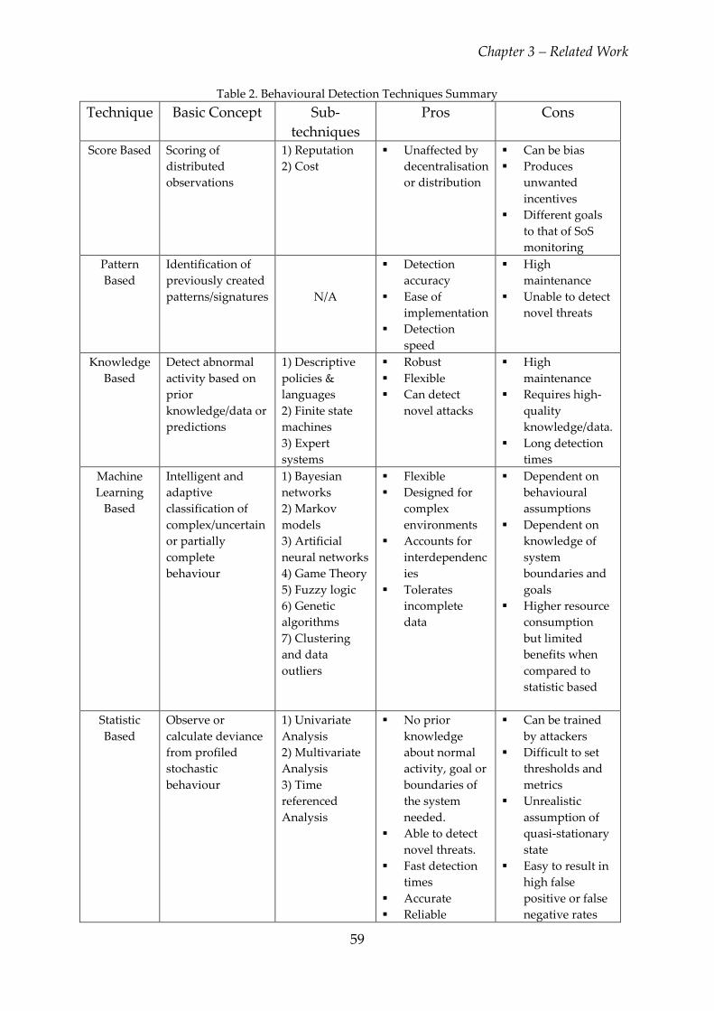


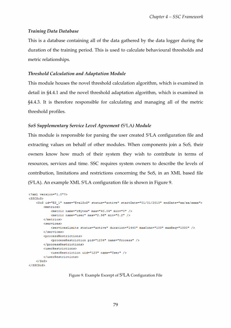


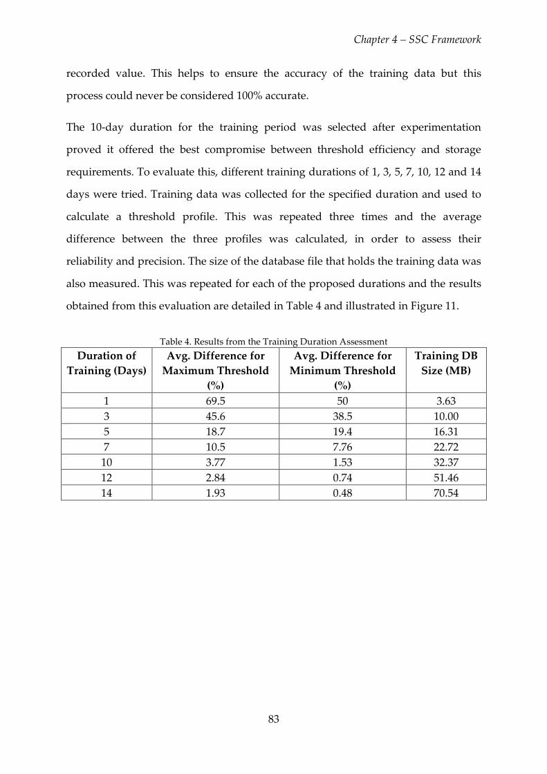
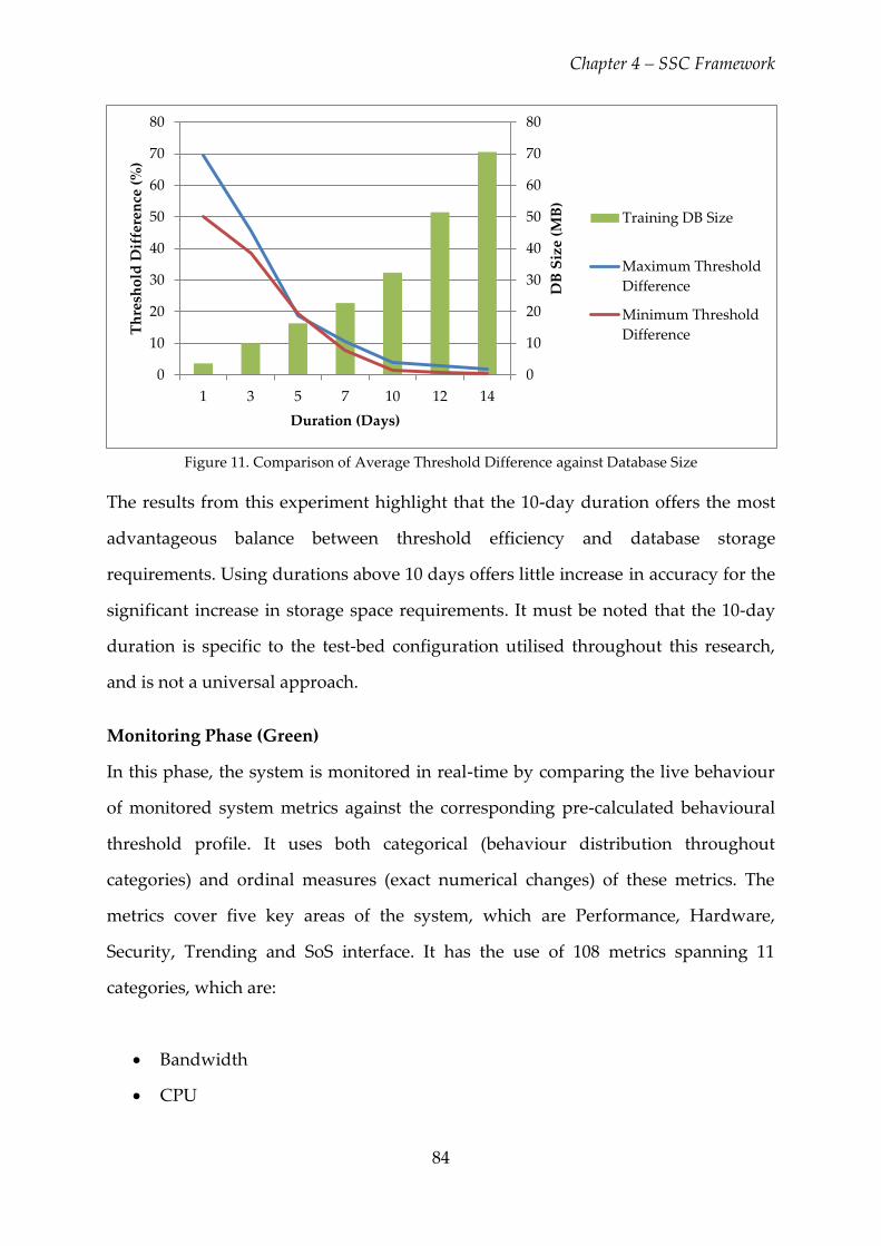


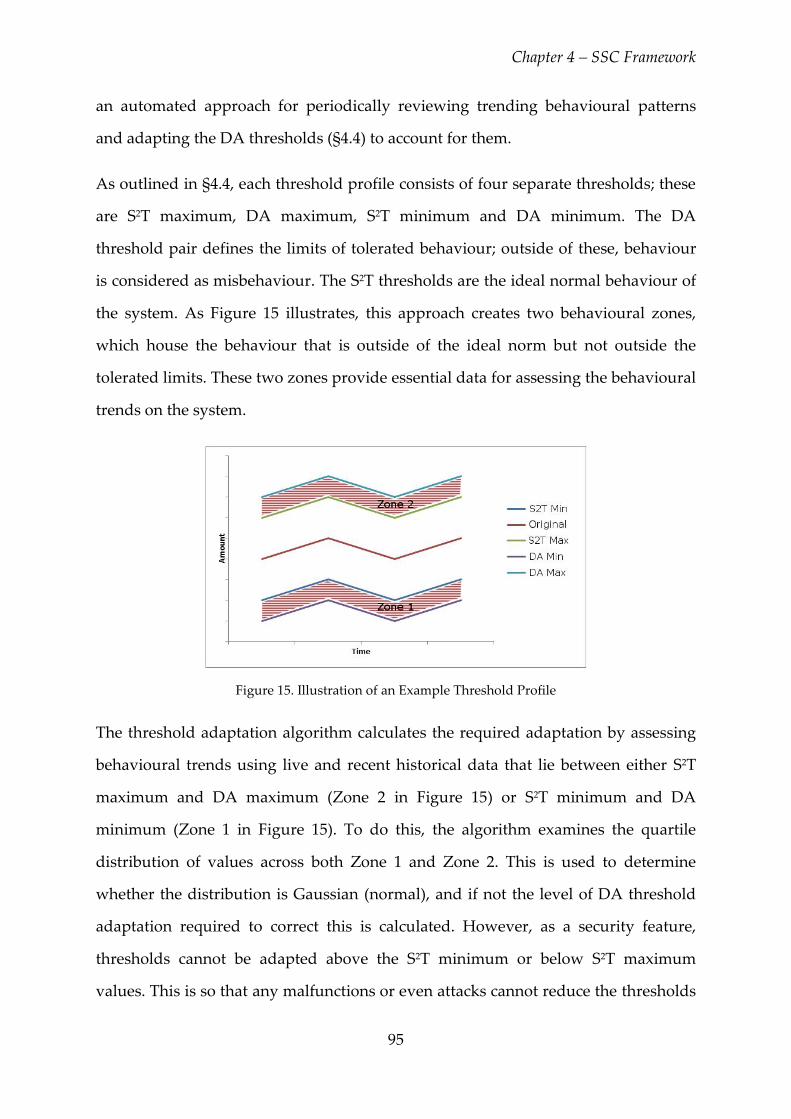


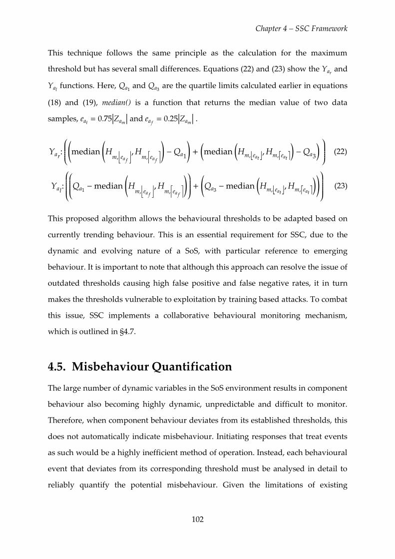


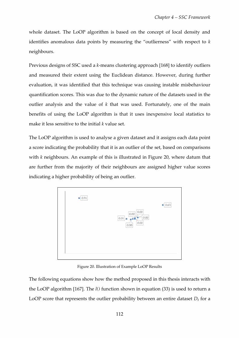


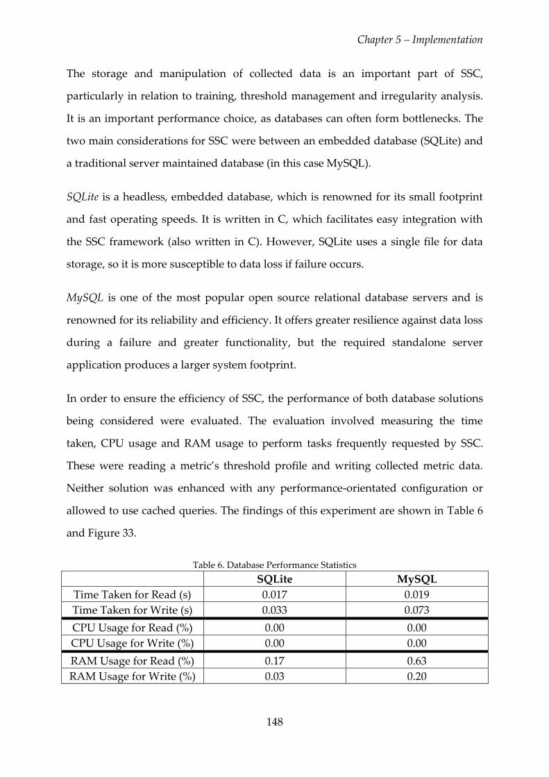
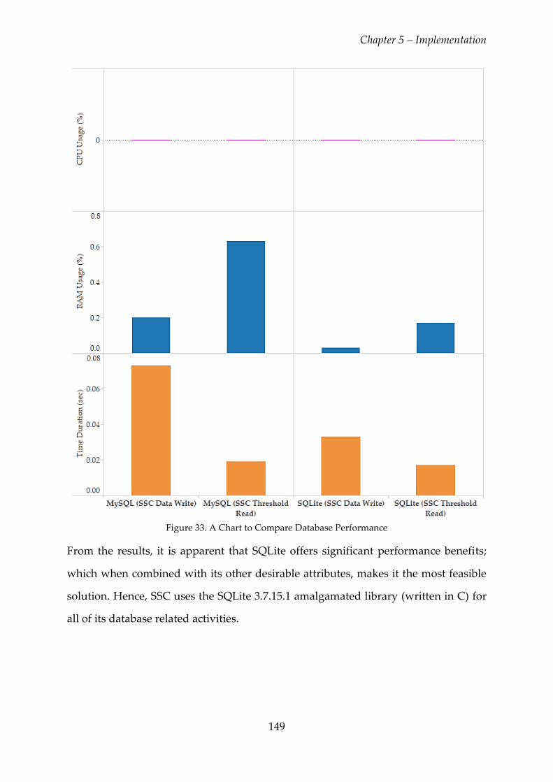

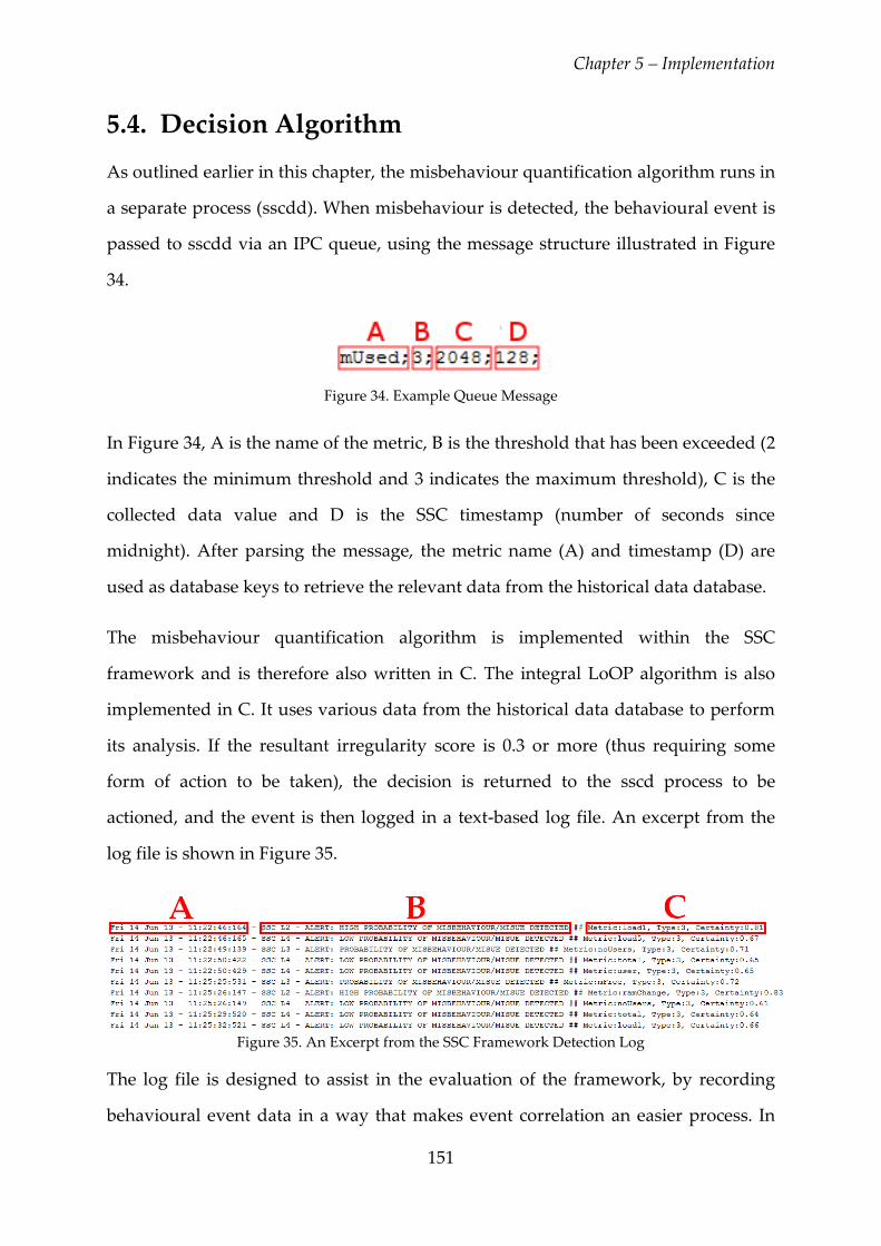


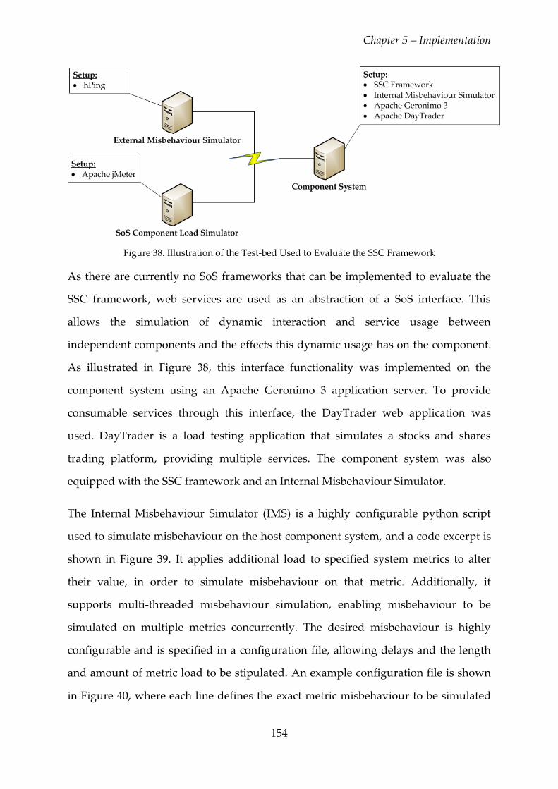


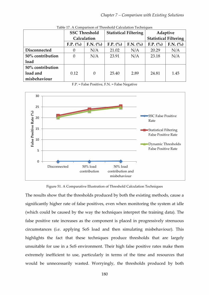


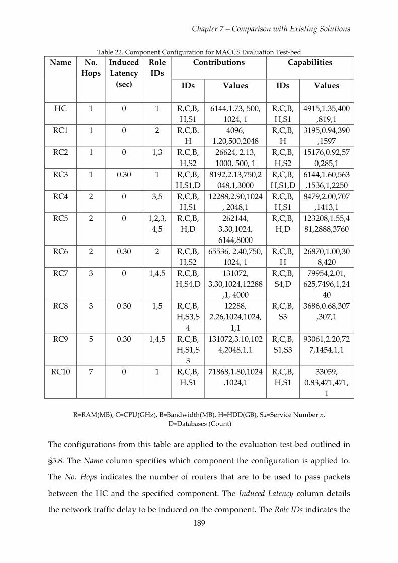

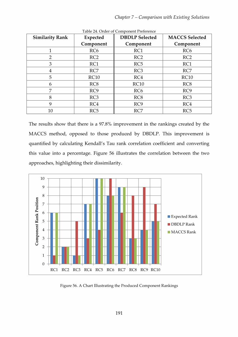

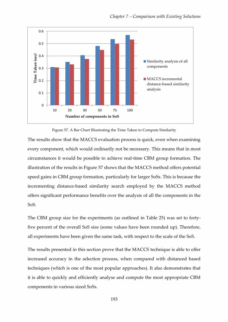


![Detecting Carbon Monoxide Poisoning Detecting Carbon ...2].pdf · Detecting Carbon Monoxide Poisoning Detecting Carbon Monoxide Poisoning. Detecting Carbon Monoxide Poisoning C arbon](https://static.documents.pub/doc/80x56/5f551747b859172cd56bb119/detecting-carbon-monoxide-poisoning-detecting-carbon-2pdf-detecting-carbon.jpg)


