DETECTION AND MODELING OF TRANSIENT AUDIO SIGNALS WITH PRIOR INFORMATION a dissertation submitted to the department of electrical engineering and the committee on graduate studies of stanford university in partial fulfillment of the requirements for the degree of doctor of philosophy Harvey Thornburg September 2005
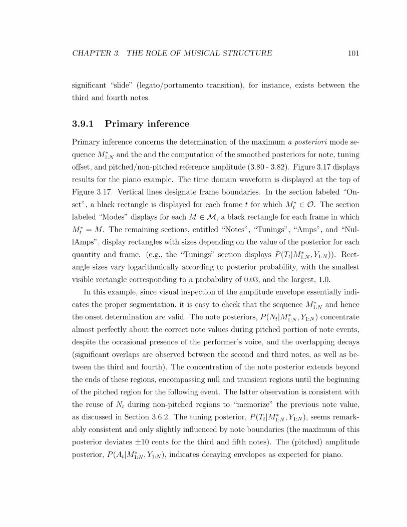
Transcript
DETECTION AND MODELING OF TRANSIENT AUDIO
SIGNALS WITH PRIOR INFORMATION
a dissertation
submitted to the department of electrical engineering
4.9 Likelihood evaluation results for exact enumeration, MCMC approxi-
mation, and MQ-initialization for piano example . . . . . . . . . . . 152
4.10 Range of P (L) given φsurv = 0.95, λspur = 3.0 for No = Ni ∈ 1:10 . . 155
A.1 Directed acyclic graph for the factorization of P (M1:N , S1:N , Y1:N) . . 162
xv
Chapter 1
Introduction
The detection and modeling of transient phenomena in musical audio signals is a
long-standing problem with applications in areas as diverse as analysis-based sound
modification, lossy audio compression, and note segmentation for automated music
analysis, transcription, and performance parameter extraction. We begin by defining
“transient” in musical audio contexts and describing common transient phenomena
which occur in these contexts. We review extensively the past literature on transient
modeling, particularly in sound modification and compression applications which use
sinusoidal models; additionally, we introduce a model for attack transients which
hybridizes sinusoidal and source-filter modeling to facilitate novel, transient-specific
processing methodologies.
Most of these modeling applications, we find, concern essentially two types of
transient phenomena: abrupt changes in spectral information, usually associated with
musical onsets, and transient regions, during which spectral information undergoes
persistent, often rapid, change. To apply transient models, therefore, we must be able
to detect abrupt changes and identify transient region boundaries. These detection
tasks become quite challenging for real-world musical signals. For instance, consider
the class of nominally monophonic recordings; here, each is considered to have been
generated from a monophonic score. Nominally monophonic recordings often contain
significant interference as well as effective polyphony due to reverberation, overlap-
ping notes, and background instrumentation, all of which increase the possibility of
1
CHAPTER 1. INTRODUCTION 2
detection errors. On the other hand, musical signals are highly structured – both
at the signal level, in terms of the spectrotemporal evolution of note events, and at
higher levels, in terms of melody and rhythm. These structures generate context
useful in predicting attributes such as pitch content, the presence and location of
abrupt-change transients, and the boundaries of transient regions. Perhaps the key
contribution of this dissertation is the integration of these contextual predictions with
raw signal information in a Bayesian probabilistic framework, in order to minimize the
expected costs associated with errors which arise in transient detection. We present
not a single solution for one set of recording conditions, but an entire framework in
which musical domain knowledge may be systematically encoded (via prior or tran-
sitional probability distributions) and adapted for a wide variety of applications and
contexts.
1.1 Definition of “transient”
Both analysis-based sound modification and lossy audio compression make extensive
use of sinusoidal models. Traditional approaches include the phase vocoder [41, 90],
as well as methods based on short-time Fourier transform (STFT) analysis and peak-
picking [81, 110, 106]1. A primary reason for its widespread use is that the sinusoidal
model offers an explicitly parametric representation of a sound’s time-frequency evo-
lution. The sinusoidal model for input yt, t ∈ 1:N is given as follows:
yt =
p∑
k=1
Ak(t) cos
(
φk(t) +
t−1∑
s=0
ωk(s)
)
(1.1)
Here Ak(t) is the amplitude of the kth sinusoid, ωk(t) is the frequency, and φk(t) is
the phase offset2. Since the time-frequency paradigm, at least to first approximation,
1The method proposed in [106] by Serra and Smith, called “spectral modeling synthesis” (SMS),is of particular interest because it represents also the part of the signal which is not well-modeledby sinusoids. This part, known as the residual, is obtained by subtracting the sinusoidal part fromthe original signal. For lossy compression purposes, unless absolute perceptual fidelity is necessary,this residual may be modeled via filtered white noise; see also [74, 75, 77] for related applications.
2Since frequency is the time difference of phase, it is redundant to represent both frequencyand phase using time-varying functions. However, this redundancy becomes quite useful when we
CHAPTER 1. INTRODUCTION 3
reflects our “mental image” of sound [53, 44], sinusoidal models help us apply musical
intuition towards designing interesting and meaningful sound modification schema.
Furthermore, most regions in typical musical audio signals are considered steady-state
with respect to the sinusoidal representation; in other words, these regions may be
represented using either constant or slowly time-varying parameter trajectories. For
compression applications, this facilitates significant reductions in bitrate with minimal
perceptual distortion [81, 77, 91, 76].
Unfortunately, real-world musical signals contain many instances, called tran-
sients, which violate these steady-state conditions. Common instances include:
• Abrupt changes in amplitudes, phases, or frequencies: in recordings of acous-
tic material, these changes are often due to energy inputs on the part of the
performer; hence, abrupt change transients often associate with onsets of note
events or other phenomena that may be notated in the score
• Rapid decays in amplitudes, usually associated with attack regions following
onsets of percussive sources
• Fast transitions in frequencies and amplitudes: musical examples include ex-
pressive pitch variations (portamento, vibrato, etc.) and timbral transitions
(such as a rapid shift in the vocal formant structure)
• Noise and chaotic regimes, primarily responsible for textural effects: environ-
mental sounds, such as rain or crackling fire, exhibit persistent textures which
are important to preserve in resynthesis; textures can also arise from nonlinear
feedback mechanisms in acoustic sources, e.g., bowed string and wind instru-
ments [103, 99]; in most circumstances, the latter are likely to be found in short
regions near onsets, as such regimes are often activated when the performer’s
energy input becomes large
What is considered “transient”, however, depends on the details of the underlying
sinusoidal model. More than one model may represent a particular signal. To cite
constrain the variation of either quantity. For instance, if frequency is modeled as piecewise-constantor piecewise-linear over short regions, the phase-offset trajectory may absorb the remainder of thelocal frequency variations which actually do occur.
CHAPTER 1. INTRODUCTION 4
an extreme case, the Fourier theorem guarantees that any signal of finite length, for
instance a sinusoidal chirp sampled at 44100 Hz for which the pitch varies linearly
from zero to 2000 Hz in 0.01 seconds, may be represented as a sum of sinusoids with
constant amplitudes, frequencies, and phases (the chirp example requiring exactly
221 sinusoids). If one wants to warp a time-varying sinusoid’s frequency trajectory,
modifying the trajectories of each individual sinusoid in the “Fourier representation”
will likely not have the desired effect. Figure 1.1 displays the results of such an
experiment with the aforementioned chirp signal where the frequencies of all Fourier
component sinusoids are doubled. Contrary to one’s expectation, the result is no
longer a single chirp, and will hence be heard as an artifact.
0 50 100 150 200 250 300 350 400 450−1
−0.5
0
0.5
1
Am
plitu
de
Before frequency−warping transformation
0 50 100 150 200 250 300 350 400 450−1
−0.5
0
0.5
1
Am
plitu
de
After frequency−warping transformation: desired result
0 50 100 150 200 250 300 350 400−1
−0.5
0
0.5
1
Time (samples)
Am
plitu
de
After frequency−warping transformation: actual result
Figure 1.1: Modification of sinusoidal chirp via stationary Fourier model
The sinusoidal modeling ambiguity manifests in more common scenarios, such as
amplitude and frequency modulation. For example, let yt be a sinusoid with zero
phase and constant frequency ω1, and time-varying amplitude At = 1 + cos(ω1t):
yt = (1 + cosω1t) cos ω0t (1.2)
CHAPTER 1. INTRODUCTION 5
But yt, as defined via (1.2), is equivalently the sum of three sinusoids with constant
parameters:
yt =1
2cos(ω0 + ω1)t +
1
2cos(ω0 − ω1)t + cos(ω0t) (1.3)
Which representation is heard depends on the relationships between ω0, ω1, and the
integration time of the ear. Generally, if |ω1 − ω0| is less than the critical bandwidth
about ω0, the result will be heard as time-varying, according to the representation
(1.2).
1.2 Modeling and detection requirements
As the discussion throughout Chapter 2 attempts to motivate, the types of transient
phenomena introduced in the previous section (abrupt changes, rapid decays, fast
timbral transitions, and noise/chaotic regimes), may for the vast majority of mod-
eling applications discussed in the literature, be combined into two types: abrupt
changes and transient regions of nonzero width. The associated detection require-
ments become as follows.
• Detect the presence of all abrupt changes, and estimate their locations
• Detect the presence of all transient regions, and estimate their beginning and
end points
Chapter 2 summarizes key applications of transient modeling in analysis-based
sound modifications which use sinusoidal models (cf. [31, 81, 93, 67, 74, 75, 68, 39, 35],
among others). In particular, time and pitch scaling3 are addressed. Since pitch scal-
ing is usually implemented by time scaling followed by sampling rate conversion [67],
we focus on time scaling. Traditional time scaling methods assume a steady-state
representation; as such, they focus on preserving the magnitudes and instantaneous
3Changing the playback speed of a recording modifies both duration and pitch; time and pitchscaling attempt to allow us independent control of each attribute. As such, time and pitch scalingare among the most well-known modification possibilities. Further definitions and relevant examplesare given in Section 2.2.1.
CHAPTER 1. INTRODUCTION 6
frequencies of each sinusoidal component in the resynthesis. In the steady-state rep-
resentation, the phase relationships become perceptually unimportant4. However, at
abrupt-change transients, the situations become reversed: phase relationships instead
play vital roles in the perception of these events whereas instantaneous frequency rela-
tionships become less important [93, 39]. Additionally, for high-fidelity applications,
it becomes necessary to either preserve or guarantee appropriate scaling of instanta-
neous magnitude time differences [93]. Failure to preserve phase relationships (and to
a lesser extent magnitude time differences) may generate audible artifacts in resyn-
thesis. In Section 2.2.3, we illustrate the importance of phase relationships at the
abrupt-change transient boundary using the simple example of a sub-audio impulse
train. This impulse train is normally heard as a series of “ticks”. Simply by modifying
phase relationships, we can generate entirely different-sounding results ranging from
sinusoidal chirps to noise textures (Figure 2.8), though the instantaneous frequency
and magnitude content remains the same.
With transient regions, it becomes additionally necessary to maintain phase rela-
tionships throughout [39, 35]. By so doing, we preserve textures and other nonstation-
ary phenomena which are otherwise difficult to model. A fundamental conflict exists
between the maintenance of phase relationships throughout a contiguous region and
the appropriate scaling of magnitude time differences at the beginning of that region,
at least within the framework of existing methods; Section 2.2.4 discusses this conflict
at length. It is usually resolved in favor of preserving phase relationships [74, 35], be-
cause perceptually, this is the more important goal [35]. However, significant portions
of some signals (e.g., some percussion sources) consist entirely of transient regions.
In this case, failure to appropriately modify the initial decay envelopes will cause the
resynthesis to be perceived as “same instrument, different tempo” [35]. If one wishes
to speed up a drum loop by a factor of, say, 25 percent, failure to shorten the decay
envelopes by this amount may lead to an unnaturally “dense” resynthesis, leaving
less room for other instruments in the mix.
4This fact has been well-known in even the earliest literature on modern psychoacoustics. Theear’s insensitivity to absolute phase during steady-state portions was proposed by Ohm and givenpsychoacoustic verification by Helmholtz [98, 17].
CHAPTER 1. INTRODUCTION 7
On the other hand, these perceptual artifacts become less pronounced if transient
regions are sufficiently short [74]. If the conflict between phase relationship preserva-
tion and magnitude time-difference scaling cannot be resolved within the framework
of existing methods, one is hence motivated to seek an extended signal representation
such that the transient regions (or, the signal information necessary to reconstruct
these regions) become as short as possible. This leads down the path of source-filter
modeling [116]. To this end, a hybrid sinusoidal/source-filter representation for at-
tack transients is developed (Figure 1.2), as discussed in Section 2.3. The main idea
TRANSIENTS SINES
NOISE
(source)(filter)
OUTPUT
Figure 1.2: Hybrid sinusoidal/source-filter representation for attack transients
is that signals of effectively short duration called input residuals excite a bank of
exponentially-decaying sinusoidal oscillators (Figure 2.11). Added to these oscillators
is an output residual which for noise added during the recording process. Absent
modification, the model is perfect reconstruction; i.e., the resynthesis is identical to
the input.
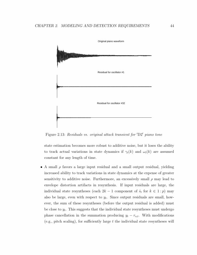
A piano attack transient and the extracted input residuals associated with the first
and 32nd partials, respectively, are displayed in Figure 1.3. The effective temporal
support of the input residuals appears substantially less than that of the input. Sec-
tion 2.3.4 discusses the improved time and pitch scaling methods facilitated by this
hybrid representation as well as some novel, “transient-specific” effect possibilities
involving residual modifications.
In summary, the discussion in Chapter 2 establishes that a tremendous variety
of transient modeling goals for analysis-based sound modification, especially those
involving sinusoidal models, require the detection and location estimation of abrupt-
change transients, and the identification of beginning and end points of transient
regions. These detection capabilities find use as well in lossy audio compression. For
CHAPTER 1. INTRODUCTION 8
Original piano waveform
Residual for oscillator #1
Residual for oscillator #32
Figure 1.3: Residuals vs. original attack transient for ′D2′ piano tone
instance, window switching [36] has helped increase the efficiency and perceptual fi-
delity of transform audio codecs (e.g., MP3, AAC) in the reproduction of transient
sound material [16, 15, 120, 14]. At least two reasons exist for the efficacy of window
switching. First, the spectral content of transient regions is generally broadband and
rapidly time-varying. Hence, it is appropriate to use shorter windows for these re-
gions and longer windows for the steady-state regions, because shorter windows have
less frequency resolution but more time resolution than longer windows. Second, the
asymmetric nature of temporal masking about abrupt change transients [82] makes
it necessary to limit the scope of pre-echo artifacts in reconstruction by applying
shorter and possibly differently-shaped windows at these occurrences [14]. A further
application concerns lossy compression schema which allow compressed-domain mod-
ifications [74, 75]. The spectrotemporal properties of transient regions as well as the
need to preserve phase relationships throughout these regions after modification and
resynthesis imply that different encodings and modification strategies must be used
CHAPTER 1. INTRODUCTION 9
for these regions [74].
Finally, the detection of abrupt-change transients and identification of transient
regions both have direct applications in automated music analysis and performance
parameter extraction5. The main reasons concern the spectrotemporal structures
commonly associated with “note events”. Most often in acoustic recordings, abrupt-
change transients result from energy inputs or decisions on the part of the performer.
Ideally, we would like to say that abrupt changes associate always with musical onsets,
defined as the beginnings of note events, as this is often the case. Unfortunately, the
level of detail provided by most traditional score-based representations may be too
coarse to adequately represent all of the performer’s energy inputs and decisions. For
instance, consider a recording of an overblown flute. During a single notated event,
multiple pitched regions may occur due to the different regimes of oscillation. Tran-
sient regions may exist between these pitched regions because of chaotic behaviors
activated upon transitioning between oscillatory regimes [99]. Nevertheless, despite
what may or may not be explicitly notated, the navigation between oscillatory regimes
is under the performer’s control, and may hence be characterized as a sequence of
discrete decisions. Discovering these decision points provides valuable information
for performance parameter extraction, which may be of use, for instance, in driving
a physical model of the same instrument [52, 79, 29], or animating a virtual per-
former [104]. Since this low-level segmentation based on abrupt-change events and
transient regions may err on the side of too much, rather than too little, detail for
score extraction purposes, this information may be clustered in a subsequent pass.
As Chapter 3 discusses, the transient detection problem may be considered jointly
with note segmentation. Particularly in the violin examples analyzed in Section 3.9,
ornamentations such as portamento and vibrato do not cause extraneous detail in the
note segmentation.
5Perhaps the primary difference in detection requirements for automated music analysis andperformance parameter extraction is that less temporal accuracy may be required for music analysistasks when compared with applications in analysis-based sound modification and audio compression;see the beginning of Section 3.10 and also 3.10.2 for further details.
CHAPTER 1. INTRODUCTION 10
1.3 The role of musical structure in transient de-
tection
With sufficiently complex musical signals, the transient detection tasks required for
the modeling applications summarized in the previous section may be difficult to
reliably perform. Even restricting to simpler cases such as nominally monophonic
signals (which may be considered as lead melodies, arising from monophonic scores),
we encounter difficulties such as noise, interference, and effective polyphony due to
background instrumentation, overlapping notes, and reverberation. These difficulties
may lead to false alarms or missed detections for both abrupt-change events and
transient regions, as well as estimation errors in the locations of abrupt-change events
and transient region boundaries.
On the other hand, musical signals are highly structured; both at the signal level,
in terms of the spectrotemporal evolution of note events, and at higher levels, in terms
of melody and rhythm. This structure manifests by constraining what is possible con-
cerning attributes such as pitch content or the presence and location of abrupt-change
events and transient region boundaries. These tendencies generate contextual predic-
tions regarding these attributes; such predictions may be combined with raw signal
information to improve detection and estimation capabilities in ways that are robust
to uncertainties in this contextual knowledge and noise in the signal. For instance,
Sections 3.3.2 and 3.3.3 demonstrate how the consistency of pitch information dur-
ing steady-state regions of note events influences our ability to detect abrupt-change
transients associated with note onsets. The beginning of Section 3.3 as well as Sec-
tion 3.10.1 discusses the role of melodic expectations, while Section 3.10.2 addresses
temporal expectations of note onsets due to the presence of rhythm.
Let us now demonstrate what is meant in a general sense by “the ability of contex-
tual predictions to improve estimation capabilities” using the framework of a linear
Gaussian model. This framework is useful because everything we wish to demon-
strate follows in closed algebraic form. Suppose y1:N is an independent and identi-
cally distributed Gaussian sequence with unknown mean x and known variance σ2y ,
and consider the estimation of x. An estimate, x, is derived as a function of y1:N ; we
CHAPTER 1. INTRODUCTION 11
want this estimate to be “best” in the sense that it minimizes the expected squared
error, E|x − x|2.A well-known lower bound on the expected squared error; i.e., the Cramer-Rao
bound [26] applies in this case:
E|x − x|2 ≥ σ2y/N (1.4)
It is easily shown (in this example) that the Cramer-Rao bound is achieved by xMLE :
xMLE = argmaxx
p(y1:N |x, σ2y)
=1
N
N∑
t=1
yt (1.5)
where p(y1:N |x, σ2y) is the conditional probability density function of the observations
given x and σ2y .
If conditions are such that σ2y/N becomes unacceptably large, (1.4) indicates that
nothing further can be done with the current set of observations, since no estimator
exists with less mean square error. Nevertheless, many problems contain additional
sources of information, which do not take the form of extra observations. Suppose a
context is established, where we expect that x lies “close to” some value, say x0. To
be precise, suppose that x is Gaussian with mean x0 and variance σ2x. Now construct
the following estimator:
xMAP = argmaxx
p(x|y1:N , σ2x, σ
2y)
=σ−2x0 + σ−2
y
∑Nt=1 yt
σ−2x + Nσ−2
y
(1.6)
where p(x|y1:N , σ2x, σ
2y) is the posterior density of x given the observations and variance
parameters σ2x and σ2
y . Some algebra shows that the expected squared error, E|x−x|2,
CHAPTER 1. INTRODUCTION 12
is
E|xMAP − x|2 = (σ−2x + Nσ−2
y )−1
< (Nσ−2y )−1
= σ2y/N (1.7)
The strict inequality in (1.7) holds provided that σ2x < ∞. That is, we have
constructed an estimator, given an additional source of contextual knowledge as rep-
resented by a prior distribution on x, with expected squared error less than that of
the Cramer-Rao lower bound. Hence, this example demonstrates in concrete, quanti-
tative terms, what is meant by prior contextual knowledge “extending our abilities”
to estimate unknown attributes from data. Analogous properties for the signal-level
structures encountered in musical audio signals (e.g., the consistency of pitch infor-
mation during pitched portions of note events) are derived in Section 3.3.2.
Unfortunately, the vast majority of transient detection approaches in the music
signal processing literature are fundamentally heuristic in nature. It is hence unclear
how we can adapt them to exploit contextual knowledge from musical structure in
ways which are robust to uncertainties in this knowledge. Most commonly, these
based on signal characteristics such as amplitude [102], phase [10], combined phase
and amplitude [33, 34], sinusoidal-model-residual level [74, 35], or automatically-
weighted combinations of individual features [48], to detect abrupt-change transients.
(This novelty-function approach may be adapted for the detection of transient re-
gions; cf. [35].) While these heuristic methods may be easy to implement, they are
often difficult to adapt to changing problem conditions (e.g., signal-to-noise ratio, the
expected rates of change of the signal characteristic during nominally steady-state vs.
transient regions, and so forth.) because they lack explicit models for uncertainty in
these conditions. If a method fails under certain conditions, it is difficult to ascertain
by what extent that method can be improved.
On the other hand, a variety of statistical methods have been applied to the
problem of detecting abrupt changes in spectrotemporal structure. These methods
CHAPTER 1. INTRODUCTION 13
provide robustness to uncertainties; as well, they address portability and optimality
concerns. Of note are the online (real-time) methods based on sequential hypothesis
testing; e.g., the divergence algorithm [8], the forward-backward method [5], offline
maximum-likelihood methods [111, 61], and integrated online-offline approaches [115].
Unfortunately, few applications of these techniques exist in musical audio; known
exceptions being [56, 50, 115]. Perhaps the primary reason is that these methods fail
to incorporate contextual predictions from musical structure, so that the limitations
imposed by adverse problem conditions (i.e., poor signal-to-noise ratios, complex
model structures, and limited amounts of data) may be overcome.
To this end, Chapter 3 proposes a Bayesian probabilistic framework for joint
melody extraction and note segmentation of nominally monophonic signals for which
steady-state regions have discernible pitch content6. This framework may be con-
sidered as a transcription system with additional features for transient detection. A
block diagram is shown in Figure 3.13; objectives may be summarized:
• The recording is segmented into discrete note events, possibly punctuated by
null regions. Null regions are gaps between note events containing only silence,
recording noise, or spurious events such as the performer knocking the micro-
phone, or clicks and pops from vinyl transfer. For each event, we identify its
onset time, duration, and MIDI note value.
• Note events are further segmented into transient and steady-state regions, where
applicable. Hence, we identify all abrupt-change transients which associate
with musical onsets as well as all boundaries of transient regions. Transients
resulting from spurious events are suppressed; this becomes a key robustness
consideration when dealing with musical audio.
• The system makes efficient use of prior contextual knowledge from musical struc-
ture, both at the signal level and at the level of syntax (melody and rhythm).
6To conform to real-world cases involving instruments such as piano and marimba, inharmonicityand more generally, uncertainty in harmonic structure is tolerated; see Chapter 4 for further discus-sion of the evaluation of pitch hypotheses, in particular Section 4.3.3 which addresses the modelingof uncertainties in harmonic structure.
CHAPTER 1. INTRODUCTION 14
The system proposed in Chapter 3 operates on framewise short time Fourier
transform (STFT) peak features. Use of STFT peak features substantially reduces
computations when compared against sample-accurate methods, without sacrificing
too much information relevant for note identification. Unfortunately, this limits
the segmentation’s temporal resolution to the frame rate7. A frame-accurate seg-
mentation may suffice for automatic transcription, but finer resolutions may be re-
quired for sound transformation and compression applications. Nonetheless, a frame-
accurate segmentation may facilitate subsequent sample-accurate processing. The
frame-accurate method identifies local neighborhoods where abrupt-change events
and transient region boundaries are likely to be found; moreover, it provides infor-
mation regarding pitch content before and after the segment boundary locations.
Section 3.10.4 discusses how the present methods may be extended to produce a
sample-accurate segmentation.
Contextual knowledge from musical structure is incorporated at the signal level
via consistency of pitch and amplitude information during steady-state (pitched) re-
gions of note events. In conjunction we exploit prior knowledge that the signal arises
from a monophonic score, according to a stochastic grammar governing the succession
of transient, pitched, and null signal regions, null regions representing gaps between
note events. Section 3.4 introduces the grammar while Section 3.6 provides its dis-
tributional specification. Since tempo, the amount of legato playing, and the relative
presence of transient information in each note event (among other characteristics)
vary from piece to piece, and this variation is otherwise difficult to model, we spec-
ify the grammar’s transition distribution up to a number of free parameters which
must be estimated from the observations. This estimation process, introduced in
Section 3.7.2, is based on the expectation-maximization (EM) algorithm [28].
Additionally, the system enables higher-level, melodic structures to inform the
segmentation, as introduced in Section 3.6.2. Here we represent melodic expectations
(the predictive distributions for subsequent notes based on past information) using a
first-order Markov note transition model. Unfortunately, the latter fails to capture
7For the examples shown in Section 3.9, the frame rate is 11.6 ms.
CHAPTER 1. INTRODUCTION 15
common melodic expectations which arise, e.g., in the context of Western tonal mu-
sic. Forthcoming work by Leistikow [71], based on recent music cognition literature
(cf. Narmour [85], Krumhansl [64], Schellenberg [101], and Larson and McAdams
[69], among others) addresses the Markovian probabilistic modeling of melodic ex-
pectations. The resultant models may be integrated with the present signal-level
framework. Section 3.10.1 summarizes these extensions.
To allow rhythmic structure to inform the segmentation, we may extend the
stochastic grammar representing the succession of transient, pitched, and null re-
gions; Section 3.10.2 discusses a proposed extension using probabilistic phase-locking
structures. Previous approaches to modeling rhythmic onset patterns, from recent
literature on tempo and beat induction from the audio signal (cf. [49, 51, 18, 65])
make suboptimal early decisions about onset locations as they use the detected onsets
as “observations” for the higher-level tempo models. By contrast, the probabilistic
phase-locking method introduced in Section 3.10.2 is fully integrated with signal-level
observations, in the sense that onsets (and other transient boundaries) are identified
jointly with tempo and beat information. Which is to say, not only do the detected
onset (and region boundary) patterns inform the tempo and beat induction; a reverse
path of influence is established between the tempo/beat layer and the onset detection
via temporal expectations. Moreover, the use of probabilistic phase-locking structures
in tempo and beat induction may find application in music cognition research, be-
cause each temporal expectation therein explicitly encodes the anticipation that a
certain event is about to occur. One may investigate affective qualities: for instance,
the buildup of tension from sustained anticipation.
Structurally, the proposed Bayesian framework for joint transient detection and
region segmentation relates to recent work in automatic transcription; cf. Kashino
et al. [60], Raphael [95, 96], Walmsley et al. [119], Godsill and Davy [46], Sheh and
Ellis [107], Hainsworth [51], [20, 18], and Kashino and Godsill [59], among possibly
others. Indeed, the use of Bayesian methods in automatic transcription is presently
an emerging field. Regarding modeling aspects, perhaps the most similar work is
that of Cemgil et al. [20, 18]. The authors therein propose a generative probabilistic
CHAPTER 1. INTRODUCTION 16
model for note identification in both monophonic and polyphonic cases8. Their model
contains what can be interpreted as a simplified version of the stochastic grammar
proposed in Section 3.6.2, in that a discrete (in this case binary) variable indicates
if a note is sounding at a given time. However, [20] models the transient information
in an additive sense, as filtered Gaussian noise superposed with the sinusoidal part,
paralleling the “sines plus noise” approach of SMS [106]. This clearly fails to satisfy
the detection requirements for the transient modeling applications in sound modifi-
cation and lossy audio compression as previously discussed. These applications favor
the explicit characterization of abrupt-change transients as well as the restriction of
transient information to contiguous regions within each note event. By contrast, the
stochastic grammar proposed in Section 3.6.2 yields not only a segmentation into
individual note events, but also a sub-segmentation of each event into transient and
steady-state regions.
A further innovation of the present method is the use of cost functions which
adequately represent the effects of various types of transcription errors, rather than
relying on byproducts of standard Bayesian filtering, smoothing, or Viterbi inference
techniques. As an example, it is less problematic for the locations of note onsets to
be shifted by small amounts than it is for notes to be missing or extra notes intro-
duced. By using an appropriate cost function, the solution to the decision problem
yields the transcription. Since one goal of Bayesian inference methods is to produce
sufficient statistics for decision problems, this means that the inference results may
be immediately converted into MIDI data without requiring complex heuristics in
postprocessing. A straightforward conversion process is detailed in Section 3.8. Here
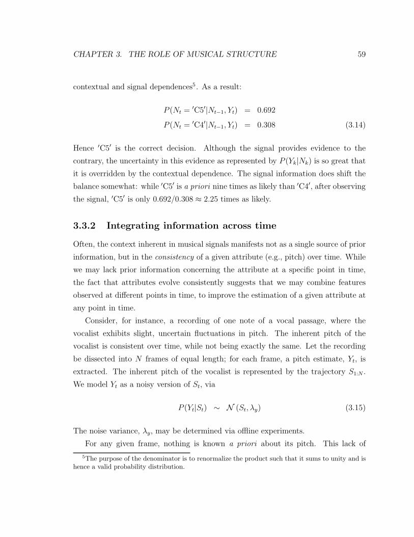
two hidden variables associate with each STFT frame: Mt, which encodes the seg-
mentation (i.e., an indication whether or not the current frame contains an onset, as
8In the framework proposed in Chapter 3, polyphonic extensions are not presently implemented.The primary reason is that the results would characterize all abrupt-change transients and transientregions for note events which overlap in time. To use these results in sound modification andcompression appliations, the transient modeling would need to perform also the source separationand demixing of individual note events which is by no means an easy task. However, the polyphonicextensions are readily applicable in performance analysis and parameter extraction. The extensionsare conceptually straightforward but may experience computational difficulties using the Bayesianinference methods discussed in Section 3.7. Section 3.10.3 provides a thorough discussion of theseissues, suggesting approximate inference schema which may greatly reduce computational costs.
CHAPTER 1. INTRODUCTION 17
well as the type of region containing this frame), and St, which encodes hidden sig-
and S1:N jointly to minimize the corresponding error probability in {M1:N , S1:N}, This
is clearly not the same thing as minimizing the probability that M1:N alone is in error
because it avoids the implicit marginalization over S1:N . Moreover, the estimated S1:N
should be synchronous with M1:N in that S1:N is chosen to satisfy some expected cost
objective under which Y1:N and M∗1:N are both entered into evidence. Inference and
estimation objectives which do satisfy these requirements are derived in Sections 3.3.3
and 3.5.2; Section 3.7.1 describes an approximate inference algorithm satisfying these
requirements.
Lastly, the present method proves robust to interference from recording noise
CHAPTER 1. INTRODUCTION 18
and actual instances of polyphony resulting from background instrumentation, note
overlaps from legato playing, and excessive reverberation. These results are demon-
strated in Section 3.9. We find that this robustness is largely due to the integration
of contextual predictions concerning the consistency of inherent pitch and amplitude
characteristics during pitched regions of note events with STFT peak observations.
For instance, suppose that a frame belonging to a pitched region of a note event is
occluded by interference. The method in this case automatically relies on the sur-
rounding frames within this region to estimate the instantaneous pitch and amplitude
characteristics for this frame, as demonstrated in Section 3.3.3. However, this robust-
ness is also partially due to the way pitch and amplitude information is extracted
from STFT peak observations, via the distributional model P (Yt|St). The quality
and robustness of this evaluation may be assessed by embedding it in a single-frame
maximum-likelihood pitch estimator, as the latter does not use information from
surrounding frames.
Chapter 4 introduces a model for evaluating P (Yt|St) based on a harmonic tem-
plate, demonstrating its use in robust maximum-likelihood pitch detection under
moderately adverse interference conditions. The harmonic template idea is intro-
duced in Section 4.2.2 and may be summarized as follows. Consider a pitch hypoth-
esis9 {f0, A0} generated from one of the possibilities for St: here f0 represents the
pitch value and A0 the corresponding (pitched) reference amplitude. The probabilis-
tic model of Chapter 4 generates a joint distribution over all frequency and amplitude
peak values potentially observed in the STFT. This model accounts for additive Gaus-
sian noise in the time domain plus uncertainties in harmonic structure resulting from
inharmonicity and other timbral variations. It may be considered an extension of the
template model in Goldstein’s probabilistic pitch detector [47], although Goldstein’s
approach ignores amplitude information.
Unfortunately, thanks to interference, we do not know which template peaks cor-
respond to peaks actually observed in the STFT. Without this linkage we cannot
evaluate P (Yt|f0, A0) via the template distributions described above. Our solution
9The necessary extension to non-pitch hypotheses, represented by the reference amplitude AQ0 ,
is discussed in Section 4.1.
CHAPTER 1. INTRODUCTION 19
is to marginalize over the unknown linkage possibility with respect to a prior (see
Section 4.3.2) favoring the survival of template peaks with a low harmonic index.
The exact marginalization, however, proves computationally intractable because the
number of linkage possibilities grows exponentially with Np where Np is the minimum
of the number of template peaks and the number of observed STFT peaks. Never-
theless, we recognize that in practice, virtually all but a few possibilities contribute
negligibly to the likelihood evaluation (see Section 4.4 for examples and further dis-
cussion). This motivates a fast Markov-chain Monte Carlo (MCMC) approximate
evaluation, developed in Section 4.5, which obtains virtually identical results for a
noisy (single-frame) piano example when compared against the exact evaluation, at
a small fraction of the computational cost. In either case, MCMC evaluation vs. ex-
act evaluation, maximum-likelihood pitch estimation yields acceptable results under
these conditions (as shown in Sections 4.4 and 4.5). On the other hand, the MCMC
evaluation may still be too slow for some applications. Alternatively, we derive a less
exact, but (in most circumstances) faster, determinstic approximation, as discussed in
Section 4.6. The computational cost of the deterministic approximation is quadratic
in Np, as opposed to the exponential cost of the exact method. This deterministic ap-
proximation is used to evaluate P (Yt|St) for the joint melody extraction and transient
detection results shown in Section 3.9.
1.4 Conclusion
In conclusion, the main contribution of this dissertation appears to be the introduction
of prior information from musical structure towards the transient detection problems
outlined above, which arise repeatedly in both established and newly introduced tran-
sient modeling contexts. Structural information is introduced both at the signal level,
in terms of the “standard note evolution” grammar, and at the level of syntax, in terms
of melodic structure. As the results of Section 3.9 demonstrate, the resultant system
for melody tracking, note onset identification and note sub-segmentation (revealing
both transient and steady-state regions within a particular note event) for nominally
monophonic musical audio appears robust to real-world interference phenomena and
CHAPTER 1. INTRODUCTION 20
actual instances of polyphony; e.g., reverberation, overlapping notes, and background
instrumentation. Moreover, because the relevant structural information is explicitly
represented using conditional probability distributions, it becomes straightforward to
adapt this system across varying musical contexts. Secondary contributions include
the robust evaluation of pitch hypotheses using a highly reduced feature set, that
of STFT peak data. This evaluation becomes useful in scenarios (e.g., maximum
likelihood pitch estimation) where prior structural information may not be readily
available, and it is easily extended to the polyphonic case as described in [72]. Ex-
tensions and further applications are discussed in Sections 3.10.1 (incorporation of
more sophisticated models of musical expectation), 3.10.2 (incorporation of temporal
expectations from rhythm via probabilistic phase-locking networks), 3.10.3 (extension
to the polyphonic case), and 3.10.4 (extension to sample-accurate segmentation and
applications in interactive audio editing).
Chapter 2
Modeling and detection
requirements
2.1 Introduction
Sinusoidal modeling is readily applicable to the analysis, transformation and resyn-
thesis of recorded sound. The main reason is that the sinusoidal model offers an
explicitly parametric representation of a sound’s time-frequency evolution. Since the
time-frequency paradigm, at least to first approximation, reflects our mental image of
sound, one may readily apply musical intuition towards specific strategies for sound
transformation.
When the realities of the signal model work contrary to musical intuition, the
result after transformation is not as expected. Here we say that artifacts occur. A
typical sinusoidal model is usually given as follows:
yt =
p∑
k=1
Ak(t) cos
(
φk(t) +
t−1∑
s=0
ωk(s)
)
(2.1)
where Ak(t) is the amplitude of the kth sinusoid, φk(t) is the phase, and ωk(t) is the
frequency at time t, where t ∈ 1:N .
Figure 2.1 depicts the usual “analysis-synthesis” framework for transforming sounds
21
CHAPTER 2. MODELING AND DETECTION REQUIREMENTS 22
via the model (2.1). In the figure, the labeling of canonical blocks analysis, transfor-
ANALYSIS TRANS-FORMATION RESYNTHESIS
PARAMETRIC SINUSOIDAL MODEL
y1:N z1:NY1:N Z1:NInput Resynthesis
Figure 2.1: Analysis, transformation, and resynthesis
mation, and resynthesis, is inspired by Serra [105]; also Pampin [86]. Analysis means
the estimation of the amplitude, phase, and frequency trajectories from the input
y1:N ; in the figure, we denote these trajectories collectively as Y1:N . Transformation
modifies these trajectories, producing Z1:N . The output, z1:N , is then resynthesized
from Z1:N , again using (2.1). We also refer to z1:N as the resynthesis.
The canonical assumption regarding the model (2.1) is that it is steady-state,
meaning that the amplitude, phase, and frequency trajectories do not vary rapidly
with time. In this way, a short time Fourier transform may be used as a front
end for the analysis, as originally proposed by Gabor [44] and adapted for digital
implementation by Portnoff [90]1.
However, musical signals contain many instances or time intervals, called tran-
sients, which violate the steady-state assumption. Transients are hence a common
source of resynthesis artifacts. We recall the types of transients defined in Section 1.1:
• Abrupt changes in amplitudes, phases, or frequencies: in recordings of acoustic
material, these changes are often due to the energy input on the part of the
1Among others, see also [31]. For a thorough overview of contemporary applications of the shorttime Fourier transform in sinusoidal modeling and music signal processing, see [108].
CHAPTER 2. MODELING AND DETECTION REQUIREMENTS 23
performer; hence, abrupt change transients often associate with onsets of note
events or other phenomena that may be notated in the score
• Rapid decays in amplitudes, usually associated with attack regions following
onsets of percussive sources
• Fast transitions in frequencies and amplitudes: musical examples include ex-
pressive pitch variations (portamento, vibrato, etc.) and timbral transitions
(such as a rapid shift in the vocal formant structure)
• Noise and chaotic regimes, primarily responsible for textural effects: environ-
mental sounds, such as rain or crackling fire, exhibit persistent textures which
are important to preserve in resynthesis; textures can also arise from nonlinear
feedback mechanisms in acoustic sources, e.g., bowed string and wind instru-
ments [103, 99]; in most circumstances, the latter are likely to be found in short
regions near onsets, as such regimes are often activated when the performer’s
energy input becomes large
What is considered “transient” depends greatly on the underlying signal model:
numerous examples are presented in Section 1.1.
2.2 Transient processing in the phase vocoder
2.2.1 Time and pitch scaling
Some of the most widespread applications of sinusoidal modeling (in the sense of
analysis-synthesis transformations) consist of time and pitch scaling and variants. It
is well known that changing the playback speed of a sound may be accomplished in
digital systems by a sampling-rate alteration; unfortunately, this operation modifies
both pitch and duration. Often we desire independent control, over these attributes.
In time scaling, the goal is to modify the sound’s duration while preserving its pitch.
This means that the amplitude and frequency trajectories for each sinusoidal compo-
nent (the parameters Ak(t) and ωk(t) in (2.1)) are interpolated over the resynthesis
CHAPTER 2. MODELING AND DETECTION REQUIREMENTS 24
time base, and φk(t) is adjusted to preserve instantaneous frequency relationships
between analysis and resynthesis. In pitch scaling, the goal is to modify the fre-
quencies of each sinusoidal component; specifically, in transposition, each frequency
is multiplied by a fixed amount. The ideal effect of each operation (playback speed
alteration, time scaling, and transposition pitch scaling) is displayed in Figure 2.2.
Since transposition is usually implemented by time scaling followed by playback speed
alteration [67], we consider only time scaling.
0 200 400 600 800 1000−1
−0.5
0
0.5
1ORIGINAL SIGNAL
0 200 400 600 800 1000−1
−0.5
0
0.5
1PLAYBACK SPEED ALTERATION
0 200 400 600 800 1000−1
−0.5
0
0.5
1TIME SCALING
0 200 400 600 800 1000−1
−0.5
0
0.5
1PITCH SCALING
Figure 2.2: Ideal resyntheses for playback speed alteration, time scaling, and pitchscaling operations
2.2.2 Phase vocoder time scaling
A common method for high quality time scaling makes use of a heterodyned filterbank
called the phase vocoder, originally developed for speech coding by Flanagan and
Golden [41], and adapted for digital implementation by Portnoff [90]. A schematic is
displayed in Figure 2.3. In the figure, j∆=
√−1.
Ideally, each component sinusoid of yt is isolated in exactly one analysis channel.
CHAPTER 2. MODELING AND DETECTION REQUIREMENTS 25
yt
L...
...
(N-1)BPF
ωc = 2π(N-1)/N
(k)ωc = 2πk/N
(0)ωc = 0
BPF
BPF
exp(-jtωc )(N-1)
exp(-jtωc )(k)
exp(-jtωc )(0)
L
L
Y(N-1)lL
Y(k)lL
Y(0)lL
Figure 2.3: Phase vocoder analysis section
This enables the time scaling process to proceed on a sinusoid-by-sinusoid basis.
Now, suppose the bandpass filters are ideal. This means, letting H(k)(ω) denote the
response of the bandpass filter for the kth channel:
H(k)(ω) =
{
1, |ω − ω(k)c | < πk
N
0, otherwise(2.2)
where ω(k)c , the channel center frequency, equals 2πk/N . Then, each channel’s output
may be reconstructed after heterodyning by e−jtω(k)c and downsampling by N , by
means of ideal sinc interpolation and subsequent modulation by ejtω(k)c . Since the
bandpass filters are generally non-ideal, their bandwidth will exceed 2πk/N and hence
a more conservative downsampling by factor L < N is advised.
To achieve time expansion by factor α, we reconstruct each Y(k)lL at instants t = lL′,
where L′ = αL, to produce the modified channel output Z(k)lL′ . If the component
is perfectly isolated by H(k)(ω) and the latter produces no phase distortion, this
component may be recovered at the frame boundaries t = lL, as Y(k)lL :
Y(k)lL
∆= ejlLω
(k)c Y
(k)lL (2.3)
CHAPTER 2. MODELING AND DETECTION REQUIREMENTS 26
according to the preceding discussion. Hence, if we define:
Z(k)lL′
∆= ejlL′ω
(k)c Z
(k)lL (2.4)
then, absent modification, the resynthesis may be taken at t = lL′ to be Z(k)lL′ . Between
these times, both the amplitude and phase of Z(k)lL′ may be interpolated to obtain Z
(k)t .
This is of course assuming the phase of Z(k)lL′ is appropriately unwrapped, which, as
we will see, is facilitated by the heterodyning process.
The resynthesis procedure is diagrammed in Figure 2.4, where the magnitude/phase
interpolation, detailed in Figure 2.5, proceeds according to the approach of McAulay
and Quatieri [81], which uses linear interpolation for the log amplitude and cubic
interpolation for the unwrapped phase2.
Y(k)lL
TRANS-FORMATION
Z(k)lL'
MAGNITUDEAND PHASE
INTERPOLATION
exp(jlL'ωc )(k)
Z(k)lL'
Z(k)tL'
Figure 2.4: Resynthesis from single channel of phase vocoder analysis
It remains to determine the mapping Y(k)lL → Z
(k)lL′ , such that the resyntheses, Z
(k)t
and Y(k)t , maintain desired relationships at frame boundaries. These relationships are
as follows [31, 68]:
• Preservation of magnitudes:
|Z(k)lL′ | = |Y (k)
lL | ∀k ∈ 0:M−1, l ∈ 1:Nl (2.5)
2Fitz et al. summarize the benefits of cubic phase interpolation for coding purposes (unmodifiedreconstruction) as follows: “In unmodified reconstruction, cubic interpolation prevents the propa-gation of phase errors introduced by unreliable parameter estimates, maintaning phase accuracy intransients, where the temporal envelope is important” [39].
CHAPTER 2. MODELING AND DETECTION REQUIREMENTS 27
MAG
PHASE
log(⋅) LIN.INTERP.
lL
exp(⋅)Z(k)lL'
Z(k)
L'
CUBICINTERP.
jlLZ(k)Z(k)t
Figure 2.5: Magnitude and phase interpolation for phase vocoder resynthesis
where Nl is the number of frames.
• Preservation of frequencies:
ω(k,Z)lL′ = ω
(k,Y )lL′ ∀k ∈ 0:M−1, l ∈ 1:Nl (2.6)
where each instantaneous frequency is defined as the average per-sample change
in the unwrapped phase:
ω(k,Y )lL
∆=
1
L
(
∠Y(k)(l+1)L − ∠Y
(k)lL
)
ω(k,Z)lL′
∆=
1
L′
(
∠Z(k)(l+1)L′ − ∠Z
(k)lL′
)
(2.7)
• Maintenance of phase continuity at frame boundaries
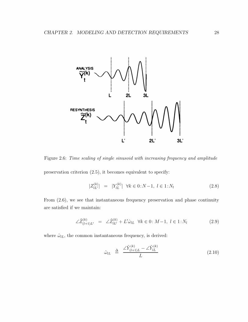
Figure 2.6 displays the time scaling of a sinusoid with linearly increasing frequency
and exponentially increasing amplitude. In the figure we observe the matching of
sinusoidal magnitudes and instantaneous frequencies across frame boundaries, as well
as the continuity of the phase in both analysis and resynthesis.
The standard phase propagation approach [83, 89, 31] maps Y(k)lL → Z
(k)lL (see Fig-
ure 2.4) in order to preserve the desired relations between Y(k)lL and Z
(k)lL . Magnitudes
and phases are treated separately. By the definitions (2.3 - 2.4) and the magnitude
CHAPTER 2. MODELING AND DETECTION REQUIREMENTS 28
Figure 2.6: Time scaling of single sinusoid with increasing frequency and amplitude
preservation criterion (2.5), it becomes equivalent to specify:
|Z(k)lL′ | = |Y (k)
lL | ∀k ∈ 0:N−1, l ∈ 1:Nl (2.8)
From (2.6), we see that instantaneous frequency preservation and phase continuity
are satisfied if we maintain:
∠Z(k)(l+1)L′ = ∠Z
(k)lL′ + L′ωlL ∀k ∈ 0: M−1, l ∈ 1:Nl (2.9)
where ωlL, the common instantaneous frequency, is derived:
ωlL∆=
∠Y(k)(l+1)L − ∠Y
(k)lL
L(2.10)
CHAPTER 2. MODELING AND DETECTION REQUIREMENTS 29
Now, from (2.3 - 2.4):
∠Yk,lL = ∠Yk,lL +2πklL
M
∠Zk,lL′ = ∠Zk,lL′ +2πklL′
M(2.11)
Substituting (2.10) and α = L′/L into (2.9), then applying (2.11) obtains:
∠Z(k)(l+1)L′ = ∠Z
(k)lL′ + α
(
∠Y(k)(l+1)L − ∠Y
(k)lL
)
(2.12)
Since analysis phases are sampled only at the frame boundaries, the role of hetero-
dyning in the phase vocoder analysis becomes clear: the heterodyned phase difference
∠Y(k)(l+1)L−∠Y
(k)lL used in the transformation (2.12) is likely to be small compared with
the actual phase difference ∠Y(k)(l+1)L−∠Y
(k)lL ; the actual difference is exactly 2πklL/M
greater than the heterodyned difference. As such, heterodyning facilitiates the req-
uisite phase unwrapping task implicit in the instantaneous frequency determination
(2.10).
2.2.3 Phase locking at the transient boundary
Unfortunately, the requirements for sound reproduction at the transient boundary [93,
39] differ somewhat with respect to the generic requirements proposed in the previous
section; i.e., instantaneous frequency/magnitude preservation and maintenance of
phase continuity at frame boundaries. For instance, suppose that frame l∗ contains
an abrupt-change transient, such as the onset of a new note event. Quatieri et al.
suggest that the following qualities of the transient’s instantaneous temporal envelope
be maintained in resynthesis:
• Preservation of magnitudes
|Z(k)lL′ | = |Y (k)
lL | ∀k ∈ 0:M−1, l ∈ 1:Nl (2.13)
• Preservation of phase relationships For all j, k ∈ 0 : M −1, wrapped phase
CHAPTER 2. MODELING AND DETECTION REQUIREMENTS 30
differences must be identical:
mod(
∠Z(k)l∗L′−∠Z
(j)l∗L′, [π, π)
)
= mod(
∠Y(k)l∗L −∠Y
(j)l∗L, [π, π)
)
(2.14)
• Appropriate scaling of magnitude time differences If one time-scales a percussive
event by a factor of two, we expect that the event will decay twice as slowly,
even initially. Hence, under scaling factor α, we desire that the per-sample time
difference of the resynthesis amplitude envelope be scaled by 1/α, immediately
after the transient boundary. In other words, we desire:
1
L′
(
|Z(k)(l∗+1)L′ |−|Z(k)
l∗L′ |)
=1
αL
(
|Y (k)(l∗+1)L|−|Y (k)
l∗L |)
∀k ∈ 0:M−1 (2.15)
The importance of preserving phase relationships as opposed to instantaneous fre-
quencies is demonstrated by the following example. Consider a bandlimited impulse
train at some sub-audio fundamental frequency, say 4 Hz. As this fundamental is
sufficiently low, the result is heard as a periodic repetition of individual “ticks”, each
comprising a distinct transient event. The impulse train may be synthesized using a
bank of sinusoidal oscillators for which each frequency is an integer multiple of the
fundamental, and all amplitudes and phases are the same, i.e.,
yt = A0
p(ω)∑
k=1
cos(kωt + φ0) (2.16)
The number of sinusoids, p(ω), is chosen such that the frequency, kω, is always less
than the Nyquist limit π rad/sample, i.e.,
p(ω) = dπ/ωe − 1 (2.17)
With φ0 = 0, ω = 5.699 · 10−4 rad/sample establishing a 4.0 Hz fundamental
at a sampling rate of 44.1 kHz , and A0 establishing a peak amplitude of 1.0, the
first 441 samples of the bandlimited impulse train are plotted in the top section
of Figure 2.7. The resyntheses displayed in the bottom sections of the figure have
CHAPTER 2. MODELING AND DETECTION REQUIREMENTS 31
0 50 100 150 200 250 300 350 400 450−0.5
0
0.5
1In−phase (zero phase)
Am
plitu
de
0 50 100 150 200 250 300 350 400 450−0.04
−0.02
0
0.02
0.04Random phase
Am
plitu
de
0 50 100 150 200 250 300 350 400 450−0.2
−0.1
0
0.1
0.2Quadratic phase
Am
plitu
de
Time (samples)
Figure 2.7: Effect of phase relationships on transient reproduction
identical amplitudes and frequencies for all sinusoidal components, but different phase
relationships:
yt = A0
p(ω)∑
k=1
cos(kωt + φk) (2.18)
In the middle section of the figure, φk is random, following a uniform distribution over
[−π, π). In the bottom section, φk = −1.0 · 10−5k2, producing a chirp with rapidly
increasing frequency. This example demonstrates the role of phase relationships to-
wards the perceived character of the transient reproduction.
To analyze the phase propagation algorithm with respect to the instantaneous
temporal envelope criteria outlined above, we recall that the magnitude preservation
is immediate from (2.8). As for the scaling of magnitude time differences, if we
CHAPTER 2. MODELING AND DETECTION REQUIREMENTS 32
multiply both sides of (2.15) by L′ and substitute the definition α = L′/L, we obtain:
|Z(k)(l∗+1)L′ | − |Z(k)
l∗L′ | = |Y (k)(l∗+1)L| − |Y (k)
l∗L | ∀k ∈ 0:M−1 (2.19)
But (2.19) is immediate from the magnitude preservation criterion (2.13).
Unfortunately, the phase propagation generally fails to preserve phase relation-
ships in the sense of (2.14). Even if (2.14) were true for a specific l∗, there is no
guarantee, unless α = 1, that this criterion will hold for subsequent frames. For
instance, suppose the first transient boundary occurs when t = 0 (frame l = 0),
and analysis phases are identically zero at this point. For this frame we may choose
the resynthesis phases to match the analysis phases, hence preserving phase relation-
ships. Now, suppose that the kth sinusoid has constant frequency ω(k). Suppose then
at t = l∗L, a second transient occurs, for which amplitudes and frequencies experi-
ence a sudden discontinuity but the phases remain continuous. In this example, the
analysis phases are as follows:
∠Y(k)l∗L = ω(k)l∗L ∀k = 0:M−1 (2.20)
Due to the phase propagation (2.9), the resynthesis phases obtain:
∠Z(k)l∗L = ω(k)l∗L′ ∀k = 0:M−1 (2.21)
From (2.20) and (2.21), it follows that analysis phase relationships are not preserved
in resynthesis. For j 6= k, the difference between analysis phases is (ω(k) − ω(j))l∗L;
the corresponding difference between resynthesis phases is (ω(k) − ω(j))l∗L′. Unless
L′ = L, meaning that there is no modification, the phase differences will fail to match
for arbitrary ω(j), ω(k), and l∗.
CHAPTER 2. MODELING AND DETECTION REQUIREMENTS 33
To remedy this, Quatieri et al. [93] propose locking resynthesis to analysis phases
at the transient boundary3; i.e.,
∠Z(k)l∗L′ = ∠Y
(k)l∗L′ (2.22)
While resetting the resynthesis phases modifies instantaneous frequencies for t ∈ (l∗−1)L′ : l∗L′, the latter becomes less problematic than modifying phase relationships in
the immediate vicinity of the transient boundary. For instance, consider the impulse
signal plotted in the top section of Figure 2.7. This signal is synthesized via (2.16)
using a fundamental frequency of 4 Hz. If instead the fundamental is 6 Hz and all
other parameters are unchanged4, the transient characteristics remain qualitatively
similar despite the 50% increase in all component frequencies. A comparison is shown
in Figure 2.8. Finally, it is important to emphasize that the phase locking at the
transient boundary, while an effective solution for reducing artifacts due to abrupt-
change transients, requires the detection of the frame l∗ in which the transient occurs.
2.2.4 Phase locking throughout transient regions
A problem with phase locking only at transient boundaries is that the lock is not
maintained during transient regions of nonzero duration unless α = 1. This is clear
from the discussion in the previous section surrounding (2.20 - 2.21). Maintaining
phase relationships throughout transient regions becomes especially important in the
resynthesis of textural sounds. Particularly problematic are textures composed of
a large collection of superposed, randomly spaced impulsive events, such as rain,
crackling fire, and so forth. Figure 2.7 displays the effects of various phase distortions
on a single impulsive event.
To this end, a number of authors, for instance Levine [74, 75], and later Duxbury
3The actual scheme is more general: it involves detecting specific groups of sinusoids whichundergo abrupt changes in amplitude, phase, or frequency characteristics. Phase locking is thenapplied individually to each group. In this way, the method can deal with more complex soundswhere transient phenomena may overlap significantly in time, but become more sparse throughouttime when restricted to particular subbands.
4The number of sinusoids, p(ω0), is also adjusted via (2.17) to avoid aliasing.
CHAPTER 2. MODELING AND DETECTION REQUIREMENTS 34
0 50 100 150 200 250 300 350 400 450−0.2
0
0.2
0.4
0.6
0.8
1In−phase resynthesis: Fundamental = 4 Hz
Am
plitu
de
0 50 100 150 200 250 300 350 400 450−0.2
0
0.2
0.4
0.6
0.8In−phase resynthesis: Fundamental = 6 Hz
Am
plitu
de
Time (samples)
Figure 2.8: Effect of frequency relationships on transient reproduction. The top figureuses a fundamental frequency of 4 Hz, the bottom uses 6 Hz. Despite the 50 % increasein all oscillator frequencies, little qualitative difference can be seen or heard
et al. [35] propose the locking of resynthesis to analysis phases at the beginning of
the transient region, as well as setting α = 1 to maintain phase locking throughout
the entire transient region. The scaling factor may be adjusted during steady-state
regions to achieve the desired resynthesis tempo which equals α times the analysis
tempo. For instance, if the input signal’s duration is 5000 samples and the desired
stretch factor equals 2.0, and the initial 1000 samples are designated as a transient
region, one specifies α = 1 for the first 1000 samples and α = 2.25 for the remainder.
One problem with this method of locking resynthesis phases to analysis phases
during transient regions is that the magnitude time differences are no longer scaled by
the inverse of the scaling factor throughout these regions. Instead, the resynthesis’s
initial decay envelope becomes identical to that for the analysis. If transient regions
are sufficiently long, the result will begin to sound like the same instrument, but
CHAPTER 2. MODELING AND DETECTION REQUIREMENTS 35
played at a different tempo. Duxbury et al. claim this as desirable: “...despite being
an ill-posed problem, it is generally agreed that when time scaling audio, the aim is for
the resulting signal to sound as if the piece is being played at a different tempo” [35].
However, this approach severely restricts the user’s ability to effect timbral changes.
Furthermore, it may generate artifacts in pitch scaling if the latter is implemented
by time scaling followed by sampling rate conversion. In pitch scaling, we expect the
initial decay rates of the resynthesis to match those of the original signal. If, instead,
these rates match after time scaling, they will no longer match after the sampling
rate conversion.
To this end, we seek a more flexible representation of transient regions within the
context of sinusoidal modeling in which the temporal support of the raw information
necessary to reconstruct these regions is as short as possible. One such representation,
introduced by the author and Leistikow [116], effectively hybridizes source-filter and
sinusoidal modeling to achieve this task. This approach relates to aspects of the
nonlinear parameter estimation by Wold [122], the Prony modeling by Laroche [66],
earlier transient modeling work by the author and Gouyon [115], spectral estimation
work by Qi et al. [92], as well as the signal-level models used in the transcription
methods of Cemgil et al. appearing around the same time [20, 19]. Section 2.3 presents
a brief overview of this hybrid sinusoidal/source-filter approach to time scaling, as
well as detailing new kinds of delay-based effects based on splitting the transient
information among different sinusoidal components.
In conclusion, essentially two types of detection are required to reduce time/pitch
scaling artifacts for sounds with significant transient content: first, the detection of
abrupt-change phenomena; second, the identification of transient regions of nonzero
width (meaning the determination of beginning and end points for these regions).
Furthermore, as the following section demonstrates, applications are by no means
limited to time and pitch scaling.
CHAPTER 2. MODELING AND DETECTION REQUIREMENTS 36
2.3 Improved transient region modeling via hybrid
sinusoidal/source-filter model
One may recall the sinusoidal modeling approaches of Levine and Smith [75], com-
monly called “transients + sines + noise”, for which the signal is segregated in time
into regions containing either transient information or “sines plus noise”. Figure 2.9
displays a schematic for this representation.
SINES + NOISE SINES + NOISE
TRANSIENT TRANSIENT
Time (frames)
Figure 2.9: “Transients + sines + noise” representation, after [75]
By contrast, [116] proposes a convolutive representation, which may be summa-
rized as “transients ? sines + noise”. Here each sinusoid consists of an exponentially
damped, quadrature oscillator which is driven by the information necessary to re-
construct the transient region. A block diagram of this approach is displayed in
Figure 2.10.
TRANSIENTS SINES
NOISE
(source)(filter)
OUTPUT
Figure 2.10: “Transients ? sines + noise”, or convolutive representation
The “transients ? sines + noise” representation facilitates the modeling of attack
transients, which consist of an abrupt-change event signifying the onset of a new note,
CHAPTER 2. MODELING AND DETECTION REQUIREMENTS 37
followed by a transient region where the sinusoidal amplitudes undergo a rapid, quasi-
exponential decay. Attack transients may also exhibit textural characteristics which
are difficult to represent by a direct sum of exponentially damped sinusoids. As later
demonstrated, the source-filter representation facilitates time-scaling modifications in
such a way that preserves textural characteristics as well as guarantees appropriate
scaling of the decay rate by the inverse of the time expansion factor, following (2.15),
because the effective temporal support of the “source” is greatly reduced with respect
to that of the original signal.
2.3.1 The driven oscillator bank
The filter (sines) component in Figure 2.10 consists of a driven oscillator bank, dis-
played in Figure 2.11. In the figure, s(I)t (k) denotes the in-phase component and
ro,tytOSCIL
St(k) s(Q)t
s(I)tr(I)i,t (k)r(Q)i,t (k)
(k)
(k)
OSCILSt(p) s(Q)t
s(I)tr(I)i,t (p)r(Q)i,t (p)
(p)
(p)
OSCILSt(k) s(Q)t
s(I)tr(I)i,t (1)r(Q)i,t (1)
(1)
(1)
INPU
T RE
SIDU
ALS
OSCILLATOR STATES
OUTPUTRESIDUAL
...
...
Figure 2.11: Driven oscillator bank
s(Q)t (k) the quadrature component of the kth oscillator at time t. The amplitude and
CHAPTER 2. MODELING AND DETECTION REQUIREMENTS 38
phase of this oscillator may be retrieved:
At(k) =
√
[
s(I)t (k)
]2
+[
s(Q)t (k)
]2
φt(k) = tan−1
[
s(Q)t (k)
s(I)t (k)
]
(2.23)
The in-phase and quadrature input residuals associated with the kth oscillator are
r(I)i,t (k) and r
(Q)i,t (k), which drive the respective oscillator states, s
(I)t (k) and s
(Q)t (k).
Starting from zero initial state for t ≤ 0, the residuals must supply the excitation for
subsequent oscillation. However, suppose r(I)t (k) and r
(Q)t (k) are identically zero for all
t ≥ T , where T is subsequent to the excitation, then the kth oscillator’s contribution
becomes for t ≥ T , a pure, exponentially decaying sinusoid. Residual contributions
which persist after the onset time contribute to non-sinusoidal qualities, such as the
perceived “texture” of the attack.
For the kth oscillator, the relation between the current oscillator state, the previous
oscillator state, and the residual at time t may be represented by the following (linear)
recursion:
[
s(I)t (k)
s(Q)t (k)
]
= eγt(k)
[
cos ωt(k) − sin ωt(k)
sin ωt(k) cos ωt(k)
][
s(I)t−1(k)
s(Q)t−1(k)
]
+
[
r(I)t (k)
r(Q)t (k)
]
(2.24)
The output, yt, sums over the in-phase oscillator states, adding a scalar output resid-
ual, ro,t:
yt =
p∑
k=1
s(I)t (k) + ro,t (2.25)
This output residual accounts for additive noise due to the recording process. It be-
comes important to distinguish additive noise from the possibly noise-like transient
information responsible for non-sinusoidal qualities of the attack, the latter encoded
by input residuals. In this way, the driven oscillator bank effectively generalizes the
CHAPTER 2. MODELING AND DETECTION REQUIREMENTS 39
canonical “sines + noise” model introduced by Serra and Smith, also known as “spec-
tral modeling synthesis” (SMS) [106], although it specializes this approach as well,
not allowing for arbitrary envelope shapes. In SMS, a single residual is obtained
by subtracting the sinusoidal resynthesis (absent modification) from the original sig-
nal. If all input residuals are identically zero except for the initial excitation, the
SMS residual equals ro,t; the present method augments this by separating residual
information inherent to the acoustic source (ri,t) from information inherent to the
recording process (ro,t). Furthermore, the association of input residuals with individ-
ual oscillators generates novel resynthesis possibilities which go beyond the canonical
time/pitch scaling paradigm; e.g., oscillator-variable delay effects. Further details
concerning these effects are discussed in Section 2.3.4.
The oscillator bank also may be viewed as a collection of second-order resonant
filters of bandpass/formant type, excited by input residuals: hence the “source-filter”
interpretation of Figure 2.10. This interpretation results from analyzing transfer
relations between r(I)i,t (k) and s
(I)t (k), and between r
(Q)i,t (k) and s
(I)t (k), since only
s(I)t (k) is observed in the output. Assuming ωt(k) and γt(k), are constant with respect
to t, taking z-transforms of both sides of (2.24) obtains as follows.
As ρ → 0, it follows from (2.41), that HKf,t+1 → 1. Substituting this limit into
(2.47) obtains Hst|1:t+1 → yt+1. As a result, (2.39), implies that ro,t → 0, as was to
be shown.
2.3.4 Analysis, transformation and resynthesis
The general analysis-transformation-resynthesis process is summarized by Figure 2.14.
• Analysis: The input signal y1:N is analyzed to extract frequency and decay
trajectories ω1:N(k) and γ1:N(k) for k ∈ 1 : p. These trajectories are converted
into the state transition matrix sequence F1:N by repeated application of (2.31).
Then y1:N and F1:N are passed to the Kalman filter consisting of the recursions
CHAPTER 2. MODELING AND DETECTION REQUIREMENTS 47
:ITERATIVE FILTERBANK(DYNAMICS ESTIMATION)
(INPUT/OUTPUT RESIDUAL
EXTRACTION)
KALMAN FILTER
INPUT OUTPUT
MODEL TRANSFORMATION RESIDUAL TRANSFORMATION
STATE−SPACE RESYNTHESIS
RESIDUAL
OUTPUT
RESIDUAL
INPUT
FREQS & DECAY RATES
RESIDUALS
RESIDUALS
FREQS & DECAY RATES
POSTPROCESSING(ENVELOPE MODIFICATION)
INPUT SIGNAL
OUTPUT SIGNAL
Figure 2.14: Block diagram for analysis-transformation-resynthesis using the hybridsinusoidal/source-filter model
(2.35, 2.36), initialized by (2.38). The Kalman filter produces the sequence of
filtered state estimates s1:N (defined via (2.34)), from which, given y1:N , the
residual sequences ri,1:N and ro,1:N are extracted via (2.39).
• Transformation The frequency and decay trajectories may be modified, along
with the residual sequences, to produce new versions of F1:N , ri,1:N , and ro,1:N .
If storage is at a premium, all but the initial excitation part of these residuals
may be discarded without too much effect on the quality of the resynthesis.
• Resynthesis The modified sequences: F1:N , ri,1:N , and ro,1:N , are presented to
the state-space model (2.30) which synthesizes a preliminary output signal. If
needed, envelope distortion artifacts caused by underspecification of the ratio
ρ∆= r/q (see Section 2.3.3) may be addressed in postprocessing which yields the
final output signal.
Extraction of the frequency and decay trajectories, γt(k) and ωt(k), is in general
a quite difficult problem for which the literature remains incomplete. Nevertheless,
there exist many special cases concerning acoustic sources for which feasible extraction
CHAPTER 2. MODELING AND DETECTION REQUIREMENTS 48
methods have been developed. For attack transients originating from quasi-harmonic
sources, for instance, the iterative filterbank method of [117] may be used. A quasi-
harmonic source obeys the following criteria [117]:
1. Frequency and decay trajectories are modeled as constant over frames. However,
variations in amplitude and phase characteristics, as encoded by the oscillator
state, may proxy for small, local variations in frequencies and decays.
2. The frequency distribution of spectral components admits a hierarchy in which
components cluster about principal harmonics. Figure 2.15 displays an example
frequency distribution. The frequency associated with the principal harmonic
0 0.5 1 1.5 2 2.5 3 3.50
0.1
0.2
0.3
0.4
0.5
0.6
0.7
0.8
0.9
1Quasi−Harmonic Signal: Distribution of Sinusoidal Frequencies
Frequency (radians)ω0
Figure 2.15: Sample frequency distribution for quasi-harmonic source
is defined as the amplitude-weighted average of all frequencies within its asso-
ciated cluster. Component frequencies assigned to a particular cluster may be
arbitrarily close.
3. Principal harmonic frequencies exist roughly about integer multiples of some
CHAPTER 2. MODELING AND DETECTION REQUIREMENTS 49
fundamental, hence the term quasi-harmonic. Even moderate amounts of in-
harmonicity are allowed, as long as the spacing between principal harmonics
varies smoothly over the entire frequency range.
Many attack transients from acoustic sources (piano, marimba, bowed string, some
bell/chime tones etc.) may be modeled as quasi-harmonic; some cannot, such as
cymbals and gongs. For more general sources the literature is by no means complete,
however Prony-based methods such as [66, 115] may be useful as long as the number
of sinusoidal components does not become too large. The advantage of methods such
as [117] as well as related “frequency zooming” work of Karjalainen et al. [58] and
Esquef et al. [37] is the use of spectral hierarchies to decompose the frequency/decay
estimation problem into a collection of smaller problems, each involving only a few
sinusoidal components.
Since input and output residuals as well as frequencies and decay trajectories
may be transformed, an almost limitless variety of resyntheses are possible using the
framework of Figure 2.14. We briefly discuss a few options relating to canonical
analysis-synthesis tasks (e.g., time and pitch scaling, cross-synthesis), as well as in-
troduce several types of effects specific to this framework, which process each residual
by different means.
• Time scaling The identified frequency and decay trajectories are resampled via
bandlimited sinc interpolation6 [109]. Each decay trajectory is then multiplied
by the inverse of the stretch factor to achieve the magnitude time difference
scaling indicated by (2.15). Input and output residuals are time scaled accord-
ing to the method discussed in Section 2.2.4, keeping in mind that the transient
regions for each residual are considerably shorter than the transient region for
the original signal. Alternatively, an ad hoc residual processing method follow-
ing [116] may be used; this method works especially well for quasi-harmonic
sources. This method defines the excitation region as the first M samples after
the onset, where M is chosen so that, averaging across all residuals, a certain
fraction of the overall residual energy is captured within the excitation region.
6If these trajectories are constant, they are extended to cover the new signal duration.
CHAPTER 2. MODELING AND DETECTION REQUIREMENTS 50
The excitation region remains unmodified, paralleling the “region locking” ap-
proach of Section 2.2.4, while the remainder of the residual is processed by
some adaptive pitch-synchronous overlap-add technique. In [116], the authors
find that the WSOLA (wave-synchronous overlap-add) protocol of Verhelst and
Roelands [118] achieves excellent results.
• Pitch scaling Transposition pitch scaling may be implemented by time scaling
followed by sampling rate conversion. However, the present method allows direct
modification of the frequency trajectories. For transposition, each trajectory is
multiplied by the transposition factor while residuals and decay trajectories
are preserved. This leads to more general types of pitch scaling effects; e.g.,
inharmonic scaling, timbre superposition (reassigning frequency components to
those obtained from a different source), and time-varying scaling, even at audio
rates.
• Cross synthesis If the analysis is performed on several sounds, residuals and
models (meaning the frequency and decay trajectories) may be interchanged.
Hybrid cross-syntheses become possible where some residuals come from one
source, and the rest from another. Furthermore, residuals extracted using dif-
ferent source-filter analyses; e.g., linear predictive coding (LPC; see [6]) may
replace the input residuals.
• Residual modifications Each input residual or groups of such may be pro-
cessed by independent means. A simple approach is to feed each pair of in-phase
and quadrature residuals corresponding to a single oscillator through an inde-
pendent delay line. If different delay times are set, this results in a splitting of
the excitation among the various harmonics, as if each harmonic were “plucked”
by a different excitation. If the delay time varies directly or inversely with fre-
quency, a “strumming” sound may be achieved. Moreover, if the independent
delay lines become regenerative, polyrhythmic textures may be superimposed
upon or seem to emerge from the original sound, creating quite striking effects.
Chapter 3
The role of musical structure
3.1 Introduction
In Chapter 1, two primary objectives are introduced for the transient detection as
applied to musical audio signals:
• First, the identification of abrupt changes in spectral content. These often arise
from a performer’s action, associating with musical onsets.
• Second, the identification of transient regions of nonzero width. Throughout
these regions, the signal fails to be “well modeled” by representations indicating
constant or slowly changing spectral content1. Transient regions are often found
near onset boundaries, for instance, during attack portions of note events.
Satisfying these objectives goes a long way towards obtaining high-quality, low-
storage analysis-based sound transformations for recordings with significant transient
1Here as in the abrupt-change designation, we are assuming some parsimonious, meaningful sig-nal representation, such as the superposition of a limited number of sinusoids with time-varyingparameters. It is these parameters, (i.e., amplitudes, frequencies, and phases), which we expect toundergo abrupt change; during transient regions we say only that no such parsimonious represen-tation may be found for which the parameters are constant or slowly varying. Of course, via thediscrete Fourier transform (DFT), one may represent any real-valued signal of finite length N withdN + 1e/2 complex sinusoidal components of constant frequencies and amplitudes. However, thisrepresentation lacks parsimony; it overfits noise elements; it is psychoacoustically and cognitivelyirrelevant and thus perceived artifacts result from most analysis-based sound transformations. SeeChapter 2 for a more involved discussion of these artifacts.
51
CHAPTER 3. THE ROLE OF MUSICAL STRUCTURE 52
content. Of particular interest are time and pitch scaling transformations. In Chap-
ter 2, we discuss phase-vocoder and sinusoidal-modeling approaches as proposed by
Quatieri et al. [93], Levine and Smith [75], Duxbury et al. [35]; and the hybrid
sinusoidal/source-filter representation of the author and Leistikow [117, 116]. The
latter is discussed at length in Section 2.3. Common to all these methods is the use
of abrupt-change detection or region identification to reduce perceived artifacts under
transformation.
3.2 The role of musical structure
Unfortunately, it becomes difficult to identify transient regions and points of abrupt
change for complex, heterogeneous musical sounds. Even near-optimal statistical
methods monitoring spectral change via piecewise constant autoregressive models, for
instance the online approaches of Basseville and Benveniste’s divergence algorithm [8]
and Andre-Obrecht’s forward-backward method [5], the offline approach of Svendsen
and Soong [111], and the integrated online-offline approach of the author and Gouyon
[115], may experience difficulties when presented with sufficiently complex signals.
78]) exist as to how well we can estimate signal characteristics given certain noise
levels, model complexities, and amounts of data.
To surpass these limits, we restrict the application to musical signals. Fortunately,
musical signals are highly structured, both at the signal level, in terms of the expected
timbral evolution of note events, and at higher levels, in terms of melodic and rhythmic
tendencies. These structures constrain relationships among signal parameters and
restrict their variation over time. For instance, musical signals contain many regions
exhibiting significant pitch content. Throughout these regions sinusoidal component
frequencies are close to integer multiples of some fundamental. Neglecting variations
due to inharmonicity, the frequency parameterization reduces from one parameter
per sinusoid (say, on the order of 20–60 parameters) to a single parameter encoding
fundamental frequency2. Now let us consider the general problem of estimating a
2Advantages in terms of the Cramer-Rao bound are discussed in [112].
CHAPTER 3. THE ROLE OF MUSICAL STRUCTURE 53
signal corrupted by noise. If we have a variety of nested model structures, all of
which are able to fit the signal in the absence of noise, it is well known [2] that the
model with fewest parameters exhibits the least variance in its estimation of the signal
in the presence of noise3.
As an example, we consider the estimation of a linear trend with a succession of
nested polynomial models. Let observations {Yt} , t ∈ 1:N be generated as follows:
Xt =[
1 t]
[
a
b
]
Yt ∼ N (Xt, 1) (3.1)
The objective is to estimate the “signal” Xt. The true model structure (3.1) is
unknown; hence, we postulate a variety of polynomial models for Xt:
Xp,t = Hp,tθp
Yt ∼ N(
Xp,t, σ2)
(3.2)
where σ2 is known, and
Hp,t =[
1 t t2 . . . tp−1]
(3.3)
and θ ∈ Rp. Here p represents the number of free parameters, the degree of the
polynomial fit being p − 1.
We estimate Xt by substituting the maximum-likelihood estimate of θp into (3.2).
It becomes convenient to define the vector quantities X ∈ RN ∆
= X1:N , Y ∈ RN ∆
=
Y1:N , and Xp ∈ RN ∆
= Xp,1:N , as well as the matrix Hp ∈ RN×p:
Hp∆=
[
HTp,1 HT
p,2 . . . HTp,N
]T
(3.4)
3This is essentially a restatement of Ockham’s razor: Pluralitas non est ponenda sine necessitate;“Plurality should not be posited without necessity.”[121]
CHAPTER 3. THE ROLE OF MUSICAL STRUCTURE 54
Under the conditionally Gaussian model with known variance (3.2), the maximum-
likelihood estimate is nothing but the least squares estimate θp:
θp = (HTp Hp)
−1HTp Y (3.5)
Hence the estimate of X, denoted as Xp, is PpY , where the projection matrix Pp is
defined:
Pp∆= HT
p (HTp Hp)
−1HTp (3.6)
Similarly, we define P⊥p = IN −Pp and note that Pp is the projection matrix onto the
column space of Hp; P⊥p is the projection matrix onto the orthogonal complement
of this space. The following, easily verified, properties become useful: PpPp = Pp;
TrPp = p; P⊥p P⊥
p = P⊥p ; TrP⊥
p = N − p; for p ≥ 2; PpX = X → P⊥p X = 0N×1.
Consider now the expected fits: both to the observed data Yt, and to the signal
Xt, as a function of p ∈ 2 : N . The simplest model able to capture the linear trend
has p = 2; the most complex model has p = N . Let the quality of fit to tbe observed
data be measured by the squared error with regards to Yt, summed over all samples.
Taking expectation with respect to the “true model” (3.2) yields
E ‖ Y − Xp ‖2 = TrE(
Y − Xp
)(
Y − Xp
)T
= TrE(
P⊥p Y Y T P⊥
p
)
= TrP⊥p
(
XXT + σ2IN
)
P⊥p
= TrP⊥p XXTP⊥
p + σ2TrP⊥p
= σ2(N − p) (3.7)
The final step follows from P⊥p X = 0 and TrP⊥
p = N − p.
Figure 3.1 on the left side illustrates fits of the observed data for p = 2 and for
p = N , where N = 7. With p = N , the fit is error free as predicted by (3.7). However,
the lack of error is clearly due to overfitting noise elements in the data. The fit of the
underlying trend Xt, as shown on the right side of Figure 3.1, seems better for the
CHAPTER 3. THE ROLE OF MUSICAL STRUCTURE 55
1 2 3 4 5 6 70
2
4
6
8Linear trend fit with linear model
1 2 3 4 5 6 70
2
4
6
8Linear trend fit with 7th order polynomial model
Figure 3.1: Linear vs. maximal degree polynomial fits for linear trend
p = 2 case. We can verify this analytically: the expected squared error for the fit of
Xt under p ≥ 2 is as follows:
E ‖ X − Xp ‖2 = TrE(
XXT − XXTp − XpX
T + XpXTp
)
= Tr(
XXT − XXT Pp + PpXXT + PpXXT Pp + σ2Pp
)
= σ2TrPp
= σ2p (3.8)
From (3.8), we see the expected error in fitting the underlying trend actually increases
with p. The best results are achieved when p = 2; this model has the fewest parame-
ters and is hence most constrained among all models able to fit the linear trend. In
other words, assuming nothing about the model structure when correct assumptions
can be made yields an overly complex model. The latter detracts from our ability to
extract meaningful information from noisy data.
We can see the analogy to the multiple sinusoids case: for perfectly harmonic
CHAPTER 3. THE ROLE OF MUSICAL STRUCTURE 56
signals, the “best” model recognizes that all component frequencies are integer mul-
tiples of some fundamental, using one parameter to encode all frequency values. Un-
fortunately, parameter constraints implied by real-world musical signals are seldom
representable by “hard” restrictions on the parameter space (i.e., stipulations that
parameters belong to certain subsets of the nominal space). For example, many
pitched acoustic signals, such as piano and marimba, contain significant amounts of
inharmonicity. The degrees and qualities of inharmonicity vary from instrument to
instrument. Consequently, we desire a model which encodes the general trend (that
the frequencies of sinusoidal components lie close to integer multiples of some funda-
mental), while maintaining robustness to uncertain, incompletely specified deviations
from this trend. In general, when proposing model structures for real-world signals,
we must plan for deviations and uncertainties in these structures, while controlling the
range of allowed variation. We later demonstrate that a Bayesian decision theoretic
framework proves most amenable to these considerations, especially in its capacity to
represent uncertain prior or structural knowledge.
3.3 Integrating context with signal information
In a broader sense, we recognize that musical structure creates context which is useful
in predicting attributes of interest; i.e., pitch content, the presence and location of
musical onsets, and the locations of transient regions. The main goal becomes to inte-
grate these contextual predictions with information from the signal to make optimal
decisions concerning these attributes. A schematic is shown in Figure 3.2.
What means an “optimal decision” takes on a necessarily probabilistic formula-
tion: in the simplest case, we aim to minimize the probability of decision error. More
generally, we aim to minimize expected costs (Bayes risks) arising from the various
types of hypotheses that are confused for one another.
CHAPTER 3. THE ROLE OF MUSICAL STRUCTURE 57
FEATUREEXTRACTIONCONTEXTUAL
PREDICTIONS
INTEGRATIONCENTER
INPUT SIGNAL
DECISIONS(PITCH, ONSET, TRANSIENT)
Figure 3.2: Integration of contextual predictions with signal information
3.3.1 Integrating a single predictive context
To illustrate the integration of a single predictive context with signal information in
decision frameworks, consider a hypothetical example of piano recording containing
one note. Suppose the recording is extremely noisy and the piano content barely
audible. The task is to decide whether the current note, represented by Nk, equals′C4′ or ′C5′. No other possibilities are considered.
Context arises from the fact the previous note Nk−1, equals ′B4′; considering the
composer, it is nine times as likely the ′B4′ will step into ′C5′ than leap down to ′C4′4:
P (Nk = ′C5′|Nk−1 = ′B4′) = 0.9
P (Nk = ′C4′|Nk−1 = ′B4′) = 0.1 (3.9)
Signal information is summarized in the feature Yk, an estimate of the fundamental
pitch. Yk = 350 Hz is observed. From offline experiments, it is determined:
P (Yk|Nk) = N(
toHz(Nk), 8000 Hz2)
(3.10)
Here toHz(·) converts the symbolic note value into a corresponding Hz pitch value.
4Such a statement could be verified by taking all scores produced by this composer, counting thenumber of ′B4′ → ′C5′ transitions, and dividing by the number of ′B4′ → ′C4′ plus ′B4′ → ′C5′
transitions.
CHAPTER 3. THE ROLE OF MUSICAL STRUCTURE 58
In particular, toHz(′C4′) = 262 Hz, and toHz(′C5′) = 523 Hz.
The interaction of contextual and signal information is shown via the directed
acyclic graph of Figure 3.3, representing the factorization of the joint distribution
P (Nk−1, Nk, Yk).
P (Nk−1, Nk, Yk) = P (Nk−1)P (Nk|Nk−1)P (Yk|Nk) (3.11)
While Yk alone seems to indicate that Nk = ′C4′, melodic context predicts Nk = ′C5′.
Nk YkNk-1
{{MELODICCONTEXT
SIGNALINFORMATION
Figure 3.3: Integration of melodic context with signal information
Which tendency wins out? The objective becomes to minimize the probability of error,
P (Nk 6= Nk), where Nk is the estimate of the current note based on Nk−1 and Yt.
It is easily shown [13] that the error probability minimization is equivalent to the
maximization
Nk = argmaxNk
P (Nk|Nk−1, Yk) (3.12)
The posterior probability P (Nk|Nk−1, Yk), is computed via Bayes’ rule:
P (Nk|Nk−1, Yk) =P (Nk|Nk−1)P (Yk|Nk)
∑
NkP (Nk|Nk−1)P (Yk|Nk)
(3.13)
Essentially, (3.13) states that the posterior is proportional to the product of the
CHAPTER 3. THE ROLE OF MUSICAL STRUCTURE 59
contextual and signal dependences5. As a result:
P (Nt = ′C5′|Nt−1, Yt) = 0.692
P (Nt = ′C4′|Nt−1, Yt) = 0.308 (3.14)
Hence ′C5′ is the correct decision. Although the signal provides evidence to the
contrary, the uncertainty in this evidence as represented by P (Yk|Nk) is so great that
it is overridden by the contextual dependence. The signal information does shift the
balance somewhat: while ′C5′ is a priori nine times as likely than ′C4′, after observing
the signal, ′C5′ is only 0.692/0.308 ≈ 2.25 times as likely.
3.3.2 Integrating information across time
Often, the context inherent in musical signals manifests not as a single source of prior
information, but in the consistency of a given attribute (e.g., pitch) over time. While
we may lack prior information concerning the attribute at a specific point in time,
the fact that attributes evolve consistently suggests that we may combine features
observed at different points in time, to improve the estimation of a given attribute at
any point in time.
Consider, for instance, a recording of one note of a vocal passage, where the
vocalist exhibits slight, uncertain fluctuations in pitch. The inherent pitch of the
vocalist is consistent over time, while not being exactly the same. Let the recording
be dissected into N frames of equal length; for each frame, a pitch estimate, Yt, is
extracted. The inherent pitch of the vocalist is represented by the trajectory S1:N .
We model Yt as a noisy version of St, via
P (Yt|St) ∼ N (St, λy) (3.15)
The noise variance, λy, may be determined via offline experiments.
For any given frame, nothing is known a priori about its pitch. This lack of
5The purpose of the denominator is to renormalize the product such that it sums to unity and ishence a valid probability distribution.
CHAPTER 3. THE ROLE OF MUSICAL STRUCTURE 60
knowledge in the framework of Gaussian dependences, may be represented [57]:
P (St) ∼ N(
0, ε−1)
(3.16)
where ε > 0 is arbitrarily small.
The consistency of inherent pitch over time is represented by St+1 ≈ St. As a
Gaussian dependence, this is modeled:
P (St+1|St) ∼ N (St, λs) (3.17)
It can be shown that for any λs ≥ 0, if P (S1) is specified via (3.16), and ε ↓ 0, there
exists an equivalent representation for P (St):
P (St) ∼ N(
0, ε−1t (λs, ε)
)
(3.18)
where ε−1t (λs, ε) ↓ 0.
A complete specification of the joint distribution satisfying (3.15 - 3.17) follows:
P (S1:N , Y1:N) = P (S1)P (Y1|S1)
N∏
t=2
P (St|St−1) (3.19)
The factorization (3.19) is represented by the directed acyclic graph of Figure 3.4.
St-1 St St+1... ...
Yt-1 Yt Yt+1
Figure 3.4: Directed acyclic graph for pitch consistency model across time
Let S∗t , t ∈ 1 : N be the maximized posterior for each frame, which serves as an
CHAPTER 3. THE ROLE OF MUSICAL STRUCTURE 61
estimated pitch trajectory:
S∗t = argmax
St
P (St|Y1:N) ∀t ∈ 1 : N (3.20)
If the set of possibilities for St were countable, this choice of S∗t would minimize the
expected number of frame errors. Since S1:N and Y1:N are jointly Gaussian, P (St|Y1:N)
is Gaussian and thus peaks at its mean; hence, S∗t = E(St|Y1:N), also minimizes the
mean squared error, E|S∗t −St|2. It is well known [57] that for linear Gaussian models,
the minimum mean squared error estimator becomes a weighted linear combination
of the observations; i.e.:
S∗t =
N∑
τ=1
wt,τYτ ∀t, τ ∈ 1:N (3.21)
Moreover, S∗t via (3.20) depends only on the ratio ρ
∆= λs/λy, irrespective of the
actual values of λs and λy. If ρ = 0, each St becomes an identical copy of the same
underlying parameter: in this case we expect S∗t to be the unweighted average of Yt;
i.e.,
wt,τ = 1/N ∀t, τ ∈ 1:N. (3.22)
As ρ → ∞, the dependence among {St, Yt} across different values of t vanishes; we
expect that S∗t depends only on the current observation Yt. For intermediate values
of ρ, we expect wt,τ to peak about τ = t, emphasizing observations in the immediate
neighborhood of t while discounting observations that are further away. As ρ becomes
small, we expect wt,τ to decay more gradually on both sides of t.
These assertions may be verified by obtaining a closed form expression for the pos-
terior P (St|Y1:N) in terms of Y1:N , λs, and λy. This posterior is computed recursively
over time in two passes: the filtering pass updates P (St+1|Y1:t+1) given P (St|Y1:t),
and the smoothing pass updates P (St|Y1:N) given P (St+1|Y1:N).
Using conditional independence relations implicit in the factorization (3.19), fil-
tering and smoothing recursions can be derived. The filtering recursion begins with
CHAPTER 3. THE ROLE OF MUSICAL STRUCTURE 62
the time update step, updating P (St|Y1:t) → P (St+1|Y1:t):
P (St+1|Y1:t) =
∫
P (St, St+1|Y1:t) dSt
=
∫
P (St|Y1:t)P (St+1|St, Y1:t) dSt
=
∫
P (St|Y1:t)P (St+1|St) dSt (3.23)
The measurement update follows, updating P (St+1|Y1:t) → P (St+1|Y1:t+1).
P (St+1|Y1:t+1) =P (St+1, Yt+1|Y1:t)
∫
P (St+1, Yt+1|Y1:t) dSt+1
P (St+1, Yt+1|Y1:t) = P (St+1, Y1:t)P (Yt+1|St+1, Y1:t)
= P (St+1|Y1:t)P (Yt+1|St+1) (3.24)
The filtering recursion is initialized after the first time update step with P (S1), via
(3.18). The final stage of the filtering recursion obtains P (SN |Y1:N), which is used to
initialize the smoothing recursion. The smoothing recursion updates P (St+1|Y1:N) →P (St|Y1:N):
P (St+1|Y1:t) =
∫
P (St, St+1|Y1:N) dSt+1
=
∫
P (St+1|Y1:N)P (St|St+1, Y1:N) dSt+1
=
∫
P (St+1|Y1:N)P (St|St+1, Y1:t) dSt+1
= P (St|Y1:t)
∫
P (St+1|Y1:N)
P (St+1|Y1:t)P (St+1|St) dSt+1 (3.25)
where P (St|Y1:t) and P (St+1|Y1:t) are precomputed and stored in the filtering pass.
Since all of the intermediate computations in (3.15-3.17) involve multiplication,
conditioning, and marginalization operations on Gaussian distributions, all intermedi-
ate quantities encountered in the filtering and smoothing recursions remain Gaussian.
As such, these quantities are completely specified by mean and variance parameters
and we may write filtering and smoothing recursions in terms of these parameters. To
CHAPTER 3. THE ROLE OF MUSICAL STRUCTURE 63
this end, we use the “Gaussian potential” algebra introduced by Lauritzen [70] and
generalized to the multivariate case by Murphy [84]. Letting ε → 0 in (3.16) obtains
the standard Kalman filter and Rauch-Tung-Striebel smoother discussed in [84, 57]:
P1 = 1/λy
S∗,(f)1 = y1
Pt+1 =λy (λs + Pt)
λy + λs + Pt
S∗,(f)t+1 = Pt+1
(
S∗,(f)t
λs + Pt
+yt+1
λy
)
S∗N = S
∗,(f)N
S∗t =
λs
λs + Pt
S∗,(f)t +
Pt
λs + Pt
S∗t+1 (3.26)
where
S∗,(f)t
∆= E(St|Y1:t)
Pt∆= V ar(St|Y1:t)
S∗t
∆= E(St|Y1:N) (3.27)
Defining P ′t = λ−1
y Pt, (3.26) may be rewritten in terms of ρ∆= λs/λy:
P′
1 = 1
S∗,(f)1 = y1
P′
t+1 =ρ + P
′
t
1 + ρ + P′
t
S∗,(f)t+1 = P
′
t+1
(
S∗,(f)t
ρ + P′
t
+ yt+1
)
S∗N = S
∗,(f)N
S∗t =
ρ
ρ + P′
t
S∗,(f)t +
P′
t
ρ + P′
t
S∗t+1 (3.28)
By induction, it is easily shown that there exist weights w(f)t,τ and wt,τ satisfying
CHAPTER 3. THE ROLE OF MUSICAL STRUCTURE 64
S∗,(f)t =
∑Nt=1 w
(f)t,τ Yτ and S
∗,(f)t =
∑Nt=1 wt,τYτ . Substituting these expressions into
(3.28) and equalizing coefficients obtains:
P′
1 = 1
w(f)1,τ = δ1,τ , τ ∈ 1 : N
P′
t+1 =ρ + P
′
t
1 + ρ + P′
t
w(f)t+1,τ = P
′
t+1
(
w(f)t,τ
ρ + P′
t
+ δt+1,τ
)
, ∀τ ∈ 1 : N
wN,τ = w(f)N,τ
S∗t =
ρ
ρ + P′
t
S∗,(f)t +
P′
t
ρ + P′
t
S∗t+1 (3.29)
where δt,τ is the Kronecker delta function; i.e.,
δt,τ =
{
1, t = τ
0, otherwise(3.30)
Figure 3.5 displays the behavior of wt,τ , as ρ ranges from 0 to ∞. If ρ = 0, the
weights appear uniform; this may be verified by simple substitution of ρ = 0 into
(3.29):
P′
t = 1/t
w(f)t,τ =
{
1/t, τ ≤ t
0, τ > t
wt,τ = 1/t, ∀t, τ ∈ 1 : N (3.31)
Assuming λy > 0, ρ = 0 implies λs = 0; in other words, the trajectory S1:N is
constant. Here it makes sense to weight all observations equally since each Yt is a
conditionally independent noisy observation of the same underlying parameter.
Likewise, as ρ → ∞, it is readily shown that w(f)t,τ converges for each t, τ ∈ 1 : N
CHAPTER 3. THE ROLE OF MUSICAL STRUCTURE 65
2 4 6 8 10 12 140
0.1
0.2
0.3
0.4
0.5
0.6
0.7
0.8
0.9
1
Frame number
Wei
ght
Estimation weight profiles for different values of ρ
2 4 6 8 10 12 140
0.1
0.2
0.3
0.4
0.5
0.6
0.7
0.8
0.9
1
Frame number
Wei
ght
Estimation weight profiles for different values of ρ
ρ = ∞
ρ = 1
ρ = 0 ρ = 0.2
ρ = 5
ρ = ∞
ρ = 1
ρ = 0 ρ = 0.2
ρ = 5
Figure 3.5: Estimation weight profiles for different values of ρ
to δt,τ , and that wt,τ converges to w(f)t,τ . As a result:
wt,τρ→∞→ δt,τ , ∀t, τ ∈ 1 : N (3.32)
If λy > 0 is finite, ρ → ∞ implies λs → ∞, meaning that the St become mutually
independent. The best estimate of St given all observations depends only on the
observation at time t.
Real-world scenarios require robustness to small drifts in pitch, while maintaining
consistency of pitch over time. Consequently, a good weight function emphasizes ob-
servations in the neighborhood of t and discounts observations that are further away.
Figure 3.5 shows that this type of weight function is guaranteed via the probabilistic
model (3.15 - 3.17; 3.19).
CHAPTER 3. THE ROLE OF MUSICAL STRUCTURE 66
3.3.3 Temporal integration and abrupt change detection
Now we consider an example where pitch is consistent, but punctuated by points
of abrupt change: the “legato” model shown in Figure 3.6. The change points are
pitchedpitched pitched pitched
onset
onset
onset
onset
Figure 3.6: “Legato” model for pitch consistency with points of abrupt change
interpreted as note onsets ; they occur at unknown times. Each pair of onsets bounds
a note event. Throughout note events, pitch information is salient and consistent;
this corresponds to legato playing. We note that the legato model may be considered
as a reduction of the nominally monophonic model introduced in Section 3.4. Adding
transient regions within note events and “null” regions, which represent gaps between
note events, extends the legato model to the nominally monophonic situation.
Given the segmentation (onset times), a heuristic may be devised in which all
observations within a note event are used to estimate the pitch trajectory for any
time along that event. The observations’ weighting would follow the profiles shown
in Figure 3.5; however, zero weight would be given to observations from other note
events. Unfortunately, this segmentation is unknown. If instead we had a good
estimate of the inherent pitch trajectory, we could monitor jumps in this trajectory
to determine onset times. However, at any fixed point in time, nothing is known a
priori about the inherent pitch. As a result, we have a classic “chicken/egg” dilemma
(Figure 3.7) characteristic of such segmentation problems [50].
To resolve this situation, we encode the unknown segmentation in a hidden binary
mode variable Mt ∈ {′O′, ′C′} which indicates whether or not frame t contains an
onset. If Mt = ′O′ (onset), an onset occurs in frame t, meaning that frames t−1
and t belong to different note events. In this case we do not expect St and St−1 to
CHAPTER 3. THE ROLE OF MUSICAL STRUCTURE 67
Figure 3.7: Canonical chicken-egg situation for segmentation applications
be related. Otherwise, Mt = ′C′ (continuation), indicating that frames t − 1 and t
belong to the same note event. In this case St ≈ St−1. The directed acyclic graph of
Figure 3.8 displays the complete factorization of the joint P (M1:N , S1:N , Y1:N):
P (M1:N , S1:N , Y1:N) = P (M1)P (S1|M1)P (Y1|S1)
×N∏
t=2
P (Mt|Mt−1)P (St|St−1, Mt)P (Yt|St) (3.33)
Here P (Mt+1|Mt) follows the stochastic grammar and state transition diagram
displayed in Figure 3.9. Here the main restriction is that onsets cannot occur in
adjacent frames. The ′C′ → ′O′ transition probability p, 0 < p � 1 models the
CHAPTER 3. THE ROLE OF MUSICAL STRUCTURE 68
St-1 St St+1... ...
Yt-1 Yt Yt+1
Mt-1 Mt Mt+1
Figure 3.8: Factorization of joint distribution for legato model
O
C
p
1-p
GRAMMAR
CC C, OO(legato model)
ASSUMPTIONS:-No onsets in adjacent frames-New note events are infrequent
Figure 3.9: Stochastic grammar for mode variables, legato model
expectation that onsets are sparse6. P (Mt+1|Mt) obtains in closed form:
P (Mt+1|Mt) =
0, Mt = ′O′, Mt+1 = ′O′
1, Mt = ′O′, Mt+1 = ′C′
p, Mt = ′C′, Mt+1 = ′O′
1 − p, Mt = ′C′, Mt+1 = ′C′
(3.34)
Consistency of pitch is governed by P (St+1|St, Mt+1). If Mt+1 = ′C′, St+1 depends
6The actual value of p controls the mean note event length in the legato case. The latter isapproximately (slightly greater than) 1/p frames.
CHAPTER 3. THE ROLE OF MUSICAL STRUCTURE 69
on St in the manner of (3.17), encoding the consistency hypothesis St+1 ≈ St; oth-
erwise, if Mt+1 = ′O′, St+1 is statistically independent of St. Furthermore, the fact
that V ar(St+1|Mt+1 = ′C′) = ε−1 indicates that there lacks additional information
concerning St+1, which parallels the situation in (3.18). Hence, P (St+1|St, Mt+1) is
modeled as follows:
P (St+1|St, Mt+1 = ′C′) ∼ N (St, λs)
P (St+1|St, Mt+1 = ′O′) ∼ N(
0, ε−1)
(3.35)
The prior dependences are specified as noninformative: P (M1) uniform; P (S1|M1)
via (3.16). Finally, the observation dependence, P (Yt|St), is specified via (3.15).
The joint segmentation and pitch tracking amounts to estimating all values of the
hidden variables M1:N and S1:N , given observations Y1:N . We aim to preserve the
integrity of the entire mode sequence, M1:N , by minimizing the probability that any
such error in this sequence may occur:
M∗1:N = argmin
M1:N
P (M1:N 6= M1:N ) (3.36)
Once again, following (3.12), the optimal sequence satisfying (3.36) maximizes the
joint posterior:
M∗1:N = argmax
M1:N
P (M1:N |Y1:N) (3.37)
We note that the objective (3.36) comprises an “all or nothing” approach, penal-
izing estimates which differ from the true sequence M1:N in only one frame the same
as estimates which have nothing to do with M1:N . Furthermore, for sufficiently long
sequences and under sufficiently noisy conditions, P (M∗1:N 6= M1:N ) may approach
unity. As such, it may be preferable to minimize the expected number of frame er-
rors, following the criterion used for S1:N (3.20) in the previous section. However,
a common source of error is when the true onset sample location lies infinitesimally
CHAPTER 3. THE ROLE OF MUSICAL STRUCTURE 70
close to a frame boundary, though just preceding it; here, considerable ambiguity ex-
ists concerning whether to assign the onset to the frame in which it actually occured,
or to the subsequent frame, for which the change in the spectral content regarding
the previous frame is most salient. If M1:N declares onsets in both frames, this incurs
at most one frame error; if a single onset is declared in the wrong frame, two frame
errors result. But detecting onsets in adjacent frames is disastrous for the segmen-
tation objective, especially if the results are to be used in transcription, because this
detection introduces an extra note event. By contrast, shifting the onset location by
one frame is far less objectionable. A more striking consideration is that the joint
posterior P (M1:N |Y1:N) vanishes over sequences containing onsets in adjacent frames
because P (Mt+1|Mt) assigns these instances zero probability (3.34). Any particular
decision M∗1:N exhibiting adjacent onsets will be invalid with respect to the gener-
ative model, thus the global maximum a posteriori criterion, (3.36) guarantees the
validity of all detected mode sequences. As such, (3.37) is validated as the proper
segmentation criterion.
Regarding the estimated pitch trajectory, S∗1:N , the objective remains to minimize
the expected number of frame errors, following (3.20). However, we require addi-
tionally that S∗1:N synchronize with M∗
1:N . We cannot tolerate, for instance, a sudden
jump in S∗t+1 from S∗
t if frames t and t+1 belong to the same note event. The solution
is to choose S∗1:N minimizing expected frame error rate given M∗
1:N :
S∗t = argmax
St
P (St|Y1:N , M∗1:N) (3.38)
where M∗1:N follows via (3.36).
3.4 Nominally monophonic signals and segmenta-
tion objectives
Unfortunately, real-world musical audio signals contain regions for which steady-
state pitch content is not salient. Such regions include transients, which associate
with note events, and null regions, or gaps, which separate note events. Ideally null
CHAPTER 3. THE ROLE OF MUSICAL STRUCTURE 71
regions would contain nothing but silence. More realistically, these regions consist
of recording noise, background instrumentation, reverberation tails from past events,
and so forth.
To this end, we extend the “legato model” introduced in Section 3.3.3 to incorpo-
rate transient and null regions. The result we denote as the nominally monophonic
model, represented by the cyclic succession (transient → pitched → null) depicted in
Figure 3.10. Here each note event comprises a transient region followed by a pitched,
transient
null
transient
null
note event note event
pitched pitched
{{
onset
onset
Figure 3.10: Region characterization for nominally monophonic signals
steady-state region. Null regions separate note events. The lengths of transient and
null regions may be zero, to encode a certain flexibility towards cases where these
regions may be absent: if both transient and null lengths are zero, the legato model
results. A new note event is instantiated upon crossing of the transient boundary :
either null → transient, pitched → transient, or null → pitched transitions trigger
onsets.
We note that the nominally monophonic model fails to allow multiple pitched
and transient regions within a single note event. This becomes problematic, for
instance, in overblown flute recordings, where multiple pitched regions may occur due
to the different oscillatory regimes, and where multiple transient regions may occur
due to chaotic behavior [99]. However, the lack of an explicit model for multiple
transient/pitched regions does not cause problems in practice. First, multiple-region
instances rarely occur when dealing with single acoustic sources. Second, when these
CHAPTER 3. THE ROLE OF MUSICAL STRUCTURE 72
instances do occur, the resultant segmentation using the nominally monophonic model
retains all information concerning the locations of abrupt-change events and transient
region boundaries, the only difference being that this model declares a new note
event upon the crossing of each transient boundary within the actual event. This
information may be aggregated in postprocessing, to form the actual note events (see
Figure 3.11):
transient transient
pitched
onset
pitched pitched
transient
onset
pitchedonset
onset
note event (aggregate)true onset
null
Figure 3.11: Aggregation of note events
While the nominally monophonic model represents signals which may arise from
a monophonic “score”, the intent is to be robust to various types of polyphony; e.g.,
note overlaps due to legato playing, reverberation, or background instrumentation.
These instances occur in virtually all real-world recordings regardless of whether or not
the performance originates from a monophonic score. Such robustness considerations,
given limited computational resources, suggest the use of framewise short-time Fourier
transform (STFT) peaks as a feature set. This stands in opposition to time domain
approaches which do not attempt feature reduction, such as the methods summarized
in Chapter 1 [20, 51, 18], among possibly others. The latter methods deliver a global,
sample-accurate segmentation, but at considerable computational expense. Even in
CHAPTER 3. THE ROLE OF MUSICAL STRUCTURE 73
some offline applications such as interactive audio editing (Section 3.10.4), a sample-
accurate response may be desired.
To summarize, we obtain a robust segmentation and melody transcription for
nominally monophonic signals, defined in the sense of the transient → pitched →null cyclic succession (Figure 3.10). The segmentation operates on a quite limited yet
psychoacoustically relevant feature set (framewise sequences of STFT peaks). The
result amounts to a transcription, but is more general: not only do we detect all note
onsets, values, and durations, we provide a sub-segmentation of each event indicating
the locations of transient regions as well as steady-state regions containing pitch con-
tent. While this method fails to provide a sample accurate segmentation, it facilitates
the latter in postprocessing, by isolating region boundaries to frame neighborhoods
and identifying possible pitch content before and after the true boundary sample lo-
cation. (Given the fact that a single abrupt-change event occurs, as well as signal
models before and after change, a simple offline likelihood maximization may be used
to estimate the changepoint location; see [61], chapter 11 for further details.)
3.5 Probabilistic model
3.5.1 Variable definitions
To encode the cyclic succession (Figure 3.10) as well as label onsets at the frame
level, we introduce the mode variable Mt for frames t ∈ 1:N . Mt takes on any of the
following values:
• ′OT′ – the beginning frame of a transient region, of which there can be at most
one per note event.
• ′OP′ – the beginning frame of a note event in which the first frame already
contains salient pitch content, of which there can be at most one per note
event.
• ′CT′ – the continuation of a transient region in the event the region occupies
more than one frame; must follow a previous ′CT′ or ′OT′.
CHAPTER 3. THE ROLE OF MUSICAL STRUCTURE 74
• ′CP′ – the continuation of a pitched region; must follow an ′OP′ or ′CP′.
• ′N′ – a null frame which occurs anytime after the last frame of a note event. A
null frame is followed by another null frame, or an onset (′OT′ or ′OP′).
Table 3.1 defines special groupings of modes with common characteristics. For
Figure 3.13: Block diagram of overall transcription process
The distributional specification is discussed below, in Section 3.6. Primary infer-
ence and parameter estimation methodologies are described in Section 3.8. However,
discussion of preprocessing stages (STFT; peak picking) is deferred to Section 4.2.1
because certain details regarding these stages relate to the modeling of peak frequency
and amplitude distributions, which is the central theme of that chapter.
CHAPTER 3. THE ROLE OF MUSICAL STRUCTURE 79
3.6 Distributional specifications
For the model in Figure 3.12, we must specify the priors P (M1), and P (S1|M1),
the transition dependence across frames: P (St+1, Mt+1|St, Mt), and the observation
likelihood P (Yt|St).
3.6.1 Prior
The role of the prior is to encode information about the first frame of the recording. If
it is known, for instance, that the recording begins with a note onset, we concentrate
P (M1) on O, the set of onset possibilities. In the most general case, however, such
knowledge is absent. Hence, we specify P (M1) as uniform and P (S1|M1) as factoring
independently among the components of S0:
P (S0|M0 ∈ P) = P (T0) P (N0) P (A0)
P (S0|M0 ∈ Q) = P (T0) P (N0) P (AQ0 ) (3.45)
where P (T0), P (N0), P (A0), and P (AQ0 ) are uniform.
3.6.2 Transition dependence
The transition dependence factors accordingly:
P (St+1, Mt+1|St, Mt) = P (Mt+1|Mt) P (St+1|Mt,Mt+1, St) (3.46)
It remains to specify mode and state dependences; respectively: P (Mt+1|Mt),
P (St+1|St, Mt, Mt+1).
CHAPTER 3. THE ROLE OF MUSICAL STRUCTURE 80
The mode transition dependence, P (Mt+1|Mt), is based around the following stan-
dard note evolution grammar encoding the cyclic succession depicted in Figure 3.10.
′OT′ → ′CT′, ′CP′
′OP′ → ′CP′, ′N′
′CT′ → ′CT′, ′CP′
′CP′ → ′CP′, ′N′, ′OT′, ′OP′
′N′ → ′OT′, ′OP′
(3.47)
The rationale behind this grammar is as follows. A primary governing princple
is that onsets, as they indicate the beginnings of note events, may not occur in
adjacent frames. In other words, an onset mode must be followed immediately by a
continuation or null mode:
P (Mt+1 ∈ C ∪N |Mt ∈ O) = 1 (3.48)
The latter ensures a well defined segmentation, especially when attack transients
occupy more than one frame. Additionally, each note event must have at least one
frame containing pitch content. The transition behavior adheres otherwise to the
cyclic succession (transient → pitched → null). where region lengths are modeled as
continuous valued random variables. Transient and null region lengths can be zero
whereas the pitched region length must be at least one frame. Since more than one
region may exist within a given frame, by convention we assign the mode Mt to be
the label of the rightmost region contained within that frame: see Figure 3.14.
The Markov transition diagram, displayed in Figure 3.15, encodes the standard
note evolution grammar, with additional tolerances for spurious incidents (e.g., an
attack transient followed immediately by silence). The latter may arise, for instance,
from the sudden “splicing” of recordings in the middle of note events. Solid lines
in Figure 3.15 represent transitions due to the standard note evolution grammar
while dotted lines represent transitions arising from spurious behaviors. The latter
transitions are assigned a small, fixed probability (on the order of 1 · 10−3).
CHAPTER 3. THE ROLE OF MUSICAL STRUCTURE 81
frame 1 frame 2 frame 3
pitchednull
transient
Figure 3.14: Schema for labeling frames according to the rightmost region assignment.In this example, frame 2 is labeled ′OP′ even though the majority of this frame isoccupied by a null region, and this frame also contains a transient region
The free parameters of P (Mt+1|Mt) are the transition probabilities for the stan-
dard note evolution grammar. Define:
pk|j∆= P (Mt+1 = k|Mt = j) ∀j, k ∈ M (3.49)
Then, let for each j ∈ M, Sj ⊂ M denote the set of possibilities for k for which pk|j
represents a transition probability in the standard note evolution grammar. Define
the vector θM as the collection of free parameters of P (Mt+1|Mt):
θM∆= Vec
⋃
j∈M
⋃
k∈Sj
{
pk|j
}
(3.50)
We estimate θM via the expectation-maximization (EM) algorithm [28]. Ideally,
θM is chosen to maximize the likelihood P (Y1:N |θM); however, the latter is generally
intractable due to the marginalization over the hidden trajectories M1:N , S1:N , of
which the number of possibilities grows exponentially with N . As such, the EM
algorithm encompasses iterations θ(i)M → θ
(i+1)M for which
{
θ(i)M , i ≥ 0
}
converges to
a local maximum of this likelihood; algorithm details are supplied in Section 3.7.2,
with additional derivations in Appendix B. A favorable initialization ensures rapid
convergence to the global likelihood maximum; we denote the latter as θ∗M .
CHAPTER 3. THE ROLE OF MUSICAL STRUCTURE 82
OT CT
CPOP
N
Figure 3.15: Markov transition diagram for P (Mt+1|Mt) .
To initialize the EM algorithm, we introduce a heterogeneous Poisson process
model representing the cyclic succession of a transient region of expected length NT ,
followed by a pitched region of expected length NP , followed by a null region of
expected length NN . Individual lengths are modeled as independent, exponentially
distributed random variables. Given the “rightmost region” assignment (Figure 3.14),
one may determine any transition probability in the initial value θ(0)M , as represented
by the nonzero elements in Table 3.2. Here, each term p(k)j,k denotes the probability
that the beginning of the next frame lies in a region of type y of the mth subsequent
cycle given that the beginning of the current frame lies in a region of type j, where
j, k ∈ {T, P, N}, and where T corresponds to a transient, P corresponds to a pitched,
and N corresponds to a null region. For example, if the current frame corresponds to
a pitched region, the probability that no transition occurs in the next frame is p(0)P,P .
The probability that the boundary of the next frame lies within the pitched region
of the subsequent note is p(1)P,P . Lastly, the probability of spurious transition, denoted
as ps, is set to some small, nonzero value; for instance, ps = 0.001 for the results of
CHAPTER 3. THE ROLE OF MUSICAL STRUCTURE 83
Section 3.9
Mt+1 = ′OT′ Mt+1 = ′OP′ Mt+1 = ′CT′
Mt =′OT′ 0 0 (1−ps)p
(0)T,T
Mt =′OP′ 0 0 0
Mt =′CT′ ps ps (1−3ps)p
(0)T,T
Mt =′CP′ p
(0)P,T p
(1)P,P 0
Mt =′N′ p
(0)N,T p
(1)N,P 0
Mt+1 = ′CP′ Mt+1 = ′N′
Mt =′OT′ (1−ps)(1 − p
(1)T,T ) ps
Mt =′OP′ p
(0)P,P 1 − p
(0)P,P
Mt =′CT′ (1−3ps)p
(1)T,T ps
Mt =′CP′ p
(0)P,P p
(0)P,N
Mt =′N′ 0 p
(0)N,N
Table 3.2: Generative Poisson model for the initialization of θM .
The state transition dependence, P (St+1|Mt, Mt+1, St), governs the expected con-
sistency between St and St+1 as a function of Mt and Mt+1. For instance, recalling
the legato model of Section 3.3.3, we expect pitch content (as represented by Nt and
Tt) to be highly consistent when frames t and t + 1 belong to pitched regions within
the same note event (Mt, Mt+1 ∈ P). In general, P (St+1|Mt, Mt+1, St) depends on Mt
at least through Mt ∈ P or Mt ∈ Q, as the relation between two temporally adjacent
pitched states is fundamentally different than the relation between a pitched state
following a non-pitched state7. No further dependence on Mt is assumed.
For fixed Mt, the variation of P (St+1|Mt, Mt+1, St) with respect to Mt+1 yields the
primary consideration for the detection of note region boundaries. Given Mt ∈ P,
Mt+1 = ′CP′ indicates that frames t and t + 1 belong to the same note event; hence
Nt+1, Tt+1, and At+1 are expected to be close to Nt, Tt, and At, respectively. On the
other hand, Mt+1 = ′OP′ signifies that frame t + 1 corresponds to the onset of a new
note event. Here, At+1 is independent of At, and Nt+1 depends only on Nt through
the probabilistic relation between the values of adjacent notes.
7This fact alone accounts for the diagonal links in Figure 3.12 which do not appear in thecorresponding graph (Figure 3.6) for the legato model, because in the latter every state is pitched.
CHAPTER 3. THE ROLE OF MUSICAL STRUCTURE 84
For fixed Mt, Mt+1 ∈ P, the transition behavior factors independently over the
components of St:
P (St+1|St, Mt+1 ∈ P, Mt ∈ P) = P (Tt+1|Tt, Mt+1, Mt ∈ P)
× P (Nt+1|Nt, Mt+1 ∈ P, Mt ∈ P) P (At+1|At, Mt+1 ∈ P, Mt ∈ P) (3.51)
Similar expressions result for Mt ∈ Q and Mt+1 ∈ Q, except in these cases At+1
is replaced by AQt+1, and At is replaced by AQ
t . We observe that the factoriza-
tion (3.51) assumes no a priori interdependence between state components when
Mt and Mt+1 are in evidence. In practice, such interdependence exists: for instance,
{Tt = 0.49, Nt = 60} and {Tt = 0.5, Nt = 61} refer to the same pitch hypothesis. The
latter ambiguity occurs upon portamento/legato transitions between notes as evi-
denced, for instance, in the violin recording analyzed in Section 3.9.1. Despite these
difficulties, the system correctly detects the onset of the second note in the transition,
and identifies the portamento pitch contour.
We discuss now the individual distributions on the r.h.s. of (3.51), considering
note, tuning, and amplitude, in that order. To begin, if Mt+1 = ′CP′, Mt ∈ Pwith probability one; hence, frames t and t + 1 belong to the same note event, and
Nt+1 ≈ Nt. In these cases, we choose the conditional distribution of Nt+1 given Nt
to concentrate about Nt. To express this concentration, we define the double-sided
exponential distribution:
E2 (X1, α+, α−|X0) =
c, X1 = X0
cαK(X1)−K(X0)+ , X1 > X0
cαK(X0)−K(X1)− , X0 > X1
(3.52)
where c is chosen such that the distribution sums to unity, and K(X) = k means that
X is the kth smallest element in the finite set of values for X. For Nt+1 given Nt, the
Ideally αN = 0, but we must allow some small deviation for robustness to the
case where the tuning offset approaches ±0.5, as here some ambiguity may result as
to the note value. Now, if Mt+1 ∈ Q, no information about the note is reflected in
the observations. Here we adopt the convention that Nt+1 refers to the value of the
most recent note event; upon transition to a new event, we will have memorized the
value of the previous event and can thus apply knowledge from melodic expectations
insofar as note-to-note dependences are concerned8. Hence
P (Nt+1|Nt, Mt+1 ∈ Q, Mt ∈ M) ∼ E2 (Nt+1|Nt, αN−, αN+) (3.54)
where αN+ = αN−∆= αN . Finally, we let Pnote trans(N1|N0) be the dependence where
N0 and N1 are the values of adjacent note events; if such information is absent, the
dependence is uniform over N1, independent of N0. If Mt+1 = ′OP′, the frame t + 1
is the first frame where the value of the new note event can be observed. Since Nt
memorizes the value of the previous note, the conditional distribution of Nt+1 must
follow Pnote trans(N1|N0):
P (Nt+1|Nt, Mt+1 = ′OP′, Mt ∈ M) ∼ Pnote trans (N1|N0) (3.55)
The remaining cases involve certain (Mt, Mt+1) combinations which occur with
zero probability due to the mode transition dependence (Table 3.2). These distribu-
tions do not affect the inference outcome, so we specify them to minimize computa-
tional effort (see Table 3.3).
The conditional distribution of the tuning reflects the assumption that tuning is
8Of course, the implied first-order Markov characterization of the prior melodic structure becomesseverely inadequate when considering the structural forms implied by most musics, specifically West-ern tonal music. In the latter case, more sophisticated Markov models may be developed, such asthe model of Leistikow [71], which effectively augments Nt with past notes and intervals, as wellas higher-level contextual attributes such as key, harmony, meter, harmonic rhythm, and beat posi-tion. Leistikow’s model translates melodic expectations derived from the music cognition researchof Narmour [85], Krumhansl [64], Schellenberg [101], Lerdahl [73] Larson and McAdams [69], andothers into variable first-order Markov dependences of the form Pnote trans(N1|N0), where N0, N1
are the augmented states corresponding to successive note events; see Section 3.10.1 for furtherdetails. Whereas the simple note-to-note model is not very useful in practice, the key innovation inthe memorization of Nt in non-pitched states is to demonstrate how contextual predictions on thelevel of syntax (i.e., melodic expectations) may inform detection capabilities at the signal level.
CHAPTER 3. THE ROLE OF MUSICAL STRUCTURE 86
expected to be constant, or vary only slightly throughout the recording, indepen-
dently of onsets, offsets and note events. Of course, this is not entirely true, as some
instruments exhibit a dynamic pitch envelope. Hence
P (Tt+1|Tt, Mt+1 ∈ M, Mt ∈ M) ∼ E2 (Tt+1|Tt, αT+, αT−) (3.56)
where αT+ = αT−∆= αT indicates symmetry of the expected tuning variation. If it is
known that the pitch will decay, such as in tuned percussion sources, we may adjust
αT+ < αT− to reflect this possibility.
Finally, we consider the conditional distribution of both pitched and null ampli-
tudes. The case (Mt+1 = ′CP′, Mt ∈ P) implies that At and At+1 belong to the same
note event, At+1 concentrating about At as follows:
9It may seem counterintuitive to model Amax,t and Yt as conditionally independent of At since,unconditionally speaking, Amax,t is a deterministic function of Yt. However, we wish not to introducebias by assuming specific dependences between the noise on Amax,t and the amplitude/frequencynoises on other peaks of Yt.
CHAPTER 3. THE ROLE OF MUSICAL STRUCTURE 90
Nt, Tt, At
Yt Amax,t
Figure 3.16: Observation layer dependence with Amax,t
We may interpolate between the rigid cases (A0,t = Amax,t vs. A0,t = At) by
varying σ2A between 0 and ∞. Assuming At ∈ R
+, as σ2A → 0, the pitch in-
ference P (Nt, Tt|Yt, Amax,t), becomes identical to the inference P ′ (Nt, Tt|Yt) where
P ′ (Yt|Nt, Tt, At) equals the canonical evaluation, P ∗ (Yt|f0(Nt, Tt), A0,t = At), with
A0,t = Amax,t. On the other hand, as σ2A → ∞, the pitch inference P (Nt, Tt|Yt, Amax,t)
converges to P (Nt, Tt|Yt), which is the canonical evaluation using A0,t = At, Amax,t
being ignored.
To show, we first consider σ2A → ∞; here the dependence on At vanishes:
P (Amax,t|At) → P (Amax,t). As a result, Amax,t and the collection {Yt, Nt, Tt, At}become mutually independent. Then P (Nt, Tt|Yt, Amax,t) → P (Nt, Tt|Yt), as was to
be shown.
Next we consider σ2A → 0; to begin, we note that in this case, P (Amax,t|At)
becomes impulsively concentrated about At; i.e.:
P (Amax,t|At) ∼ δ (Amax,t, At) (3.64)
It suffices to show that, given (3.64), P (Nt, Tt|Yt, Amax,t) becomes identical to the
where the double-sided exponential, E2, is defined by (3.52). The amount of consis-
tency is governed by αN in the sense that αN ↓ 0 indicates that all note values must
be identical during the entire pitched region.
In practice, it is virtually unheard of for the maxmized note posterior to fail to be
identical during the pitched portions of note events, as even extreme vibrato effects
may be absorbed by tuning offset variations. Hence, there is no loss of generality in
setting αN = 0, implying that the actual value of c0 specified in (3.90) is immaterial,
as long as c0 > 0.
CHAPTER 3. THE ROLE OF MUSICAL STRUCTURE 100
3.9 Results
The system for joint onset detection, transient region identification, and melody tran-
scription developed in the preceding sections has been applied to a variety of piano
and violin recordings. While each recording arises from a monophonic score, in ac-
tuality they contain instances of polyphony due to reverberation, note overlaps from
legato playing, and background instrumentation. Furthermore, expressive pitch vari-
ations such as portamento and vibrato occur in the violin passages. The goal of this
section is to provide a detailed analysis of the system’s performance for one repre-
sentative example of each type: a piano recording in which the performer also sings
in the background, and a violin recording exhibiting significant reverberation, legato
playing and expressive pitch variation.
The piano recording consists of the introductory motive of Bach’s Invention II in
C minor (BWV 773), performed by Glenn Gould. The top section of Figure 3.17
displays the time domain waveform. While this recording lacks significant reverber-
ation, the legato playing style nevertheless causes many notes to overlap. A further
complication is that the performer (Gould) accompanies himself with low-amplitude
vocalizations, with fundamentals approximately two octaves below those of the pi-
ano10. Nevertheless, onsets are clearly visible and may be determined by standard
heuristic time domain approaches which monitor jumps in the amplitude envelope;
see, for instance, the algorithm of Schloss [102] used in the automatic transcription of
percussive music. The purpose of this example is mainly to show robustness to low
levels of background instrumentation.
The violin recording is an excerpt from the third movement of Bach’s solo violin
Sonata No. 1 in G minor (BWV 1001), performed by Nathan Milstein. The top
section of Figure 3.18 displays the time domain waveform. This recording is awash
in reverberation, which makes it difficult to detect onsets visually or by monitoring
the amplitude envelope. Furthermore, excessive reverberation combined with legato
playing induces significant polyphony due to overlapping notes. Expressive pitch
variations, particularly portamento, create ambiguities concerning onset locations. A
10This idiosyncrasy of Gould has been well documented; see Malone [80] for an interesting studyof counterpoint with regards to the piano material as appearing in Gould’s vocalizations.
CHAPTER 3. THE ROLE OF MUSICAL STRUCTURE 101
significant “slide” (legato/portamento transition), for instance, exists between the
third and fourth notes.
3.9.1 Primary inference
Primary inference concerns the determination of the maximum a posteriori mode se-
quence M∗1:N and the and the computation of the smoothed posteriors for note, tuning
Figure 3.17: Piano example: Introductory motive of Bach’s Invention 2 in C minor(BWV 773), performed by Glenn Gould
CHAPTER 3. THE ROLE OF MUSICAL STRUCTURE 103
Corresponding results for the violin example are displayed in Figure 3.18. Since
onsets are not directly visible by eye, checking the validity of the segmentation in the
violin example becomes a painstaking process in which one must repeatedly splice
and listen to various extracts, each time shifting the possible note boundaries. This
process may take several minutes for each second of music. Further complications
arise thanks the to shortness of the segments and the significant polyphony induced
by reverberation and legato playing. Nevertheless, it seems difficult to improve on
the resultant segmentation as indicated by M∗1:N .
Through maximizing the note posterior, P (Nt|M∗1:N , Y1:N), all notes are correctly
detected except for the initial “grace note” comprising the first three frames11. For
these frames, the detected pitch is one octave below the notated pitch. The tuning
posterior is less consistent than in the piano example, primarily due to portamento.
We see that the overt slide between the third and fourth notes manifests in the drift
of the maximized tuning posterior about the onset of the fourth note.
3.9.2 Estimation of mode transition dependence
The convergence of the EM iterations for estimating P (Mt+1|Mt) is displayed in
Figure 3.19 for the Poisson initialization and in Figure 3.20 for a uniform initialization.
The latter is provided for purposes of comparison. These figures refer to the piano
example generating the primary inference results of Figure 3.17. States labeled on the
horizontal axis correspond to Mt+1; the vertical axis, Mt. Black rectangles are used
to display the transition probabilities P (Mt+1|Mt); the size of each rectangle varies
logarithmically with the probability value according to the schema of the previous
section (Figures 3.17 and 3.18). That is, the smallest visible rectangle corresponds to
a transition probability of 0.03 while the largest corresponds to a probability of 1.0.
Recall that the Poisson initialization encodes knowledge of the “cyclic succession”
schema (Figure 3.10), where a transient region of expected length NT is followed by
a pitched region of expected length NP , followed by a null region of expected length
NN , and repeating until the end of the signal. Individual region lengths are modeled
11The note in question is not an actual grace note, but an artifact due to truncation of all butthree frames from the previous note event.
CHAPTER 3. THE ROLE OF MUSICAL STRUCTURE 104
10 20 30 40 50 60 70 80 90 100 110Frames
0.0501
0.0006NullAmps
55.2931
0.6911Amps
0.41
−0.50
Tunings
80
44
Notes
N CP CT OP OT
Modes
onOnset−1.0
0.0
1.0
Signal
Figure 3.18: Primary inference results on an excerpt from the third movement ofBach’s solo violin Sonata No. 1 in G minor (BWV 1001), performed by NathanMilstein
CHAPTER 3. THE ROLE OF MUSICAL STRUCTURE 105
OT OP CT CP N
N
CP
CT
OP
OT
(a) Init
OT OP CT CP N
N
CP
CT
OP
OT
(b) Iter. 1
OT OP CT CP N
N
CP
CT
OP
OT
(c) Iter. 2
OT OP CT CP N
N
CP
CT
OP
OT
(d) Iter. 3
OT OP CT CP N
N
CP
CT
OP
OT
(e) Iter. 4
OT OP CT CP N
N
CP
CT
OP
OT
(f) Iter. 5
Figure 3.19: EM convergence results beginning from Poisson initialization
as independent, exponentially distributed random variables. We choose mean lengths
of NT = 23 ms, NP = 580 ms, and NN = 348 ms 12. The EM convergence, however,
appears relatively insensitive to modest variations in mean lengths.
The uniform initialization attempts to remove all prior knowledge from the speci-
fication of θ(0)M , distributing transition probabilities in a conditionally uniform manner
given Sj ∈ M for each j ∈ M after accounting for spurious transitions. To represent
the latter, let Sspurj denote for each j ∈ M, the collection of k ∈ M for which the
j → k transition is spurious, meaning that it appears as a dotted line in Figure 3.15.
Then, according to (3.83), we may represent θ(0)M as follows:
θ(0)M
∆= Vec
⋃
j∈M
⋃
k∈Sj
{
p(0)k|j
}
(3.93)
12With 44100 Hz sampling rate and 1024-sample frames, these settings are achieved with NT = 1frame, NP = 25 frames, and NN = 15 frames.
CHAPTER 3. THE ROLE OF MUSICAL STRUCTURE 106
OT OP CT CP N
N
CP
CT
OP
OT
(a) Init
OT OP CT CP N
N
CP
CT
OP
OT
(b) Iter. 1
OT OP CT CP N
N
CP
CT
OP
OT
(c) Iter. 2
OT OP CT CP N
N
CP
CT
OP
OT
(d) Iter. 3
OT OP CT CP N
N
CP
CT
OP
OT
(e) Iter. 4
OT OP CT CP N
N
CP
CT
OP
OT
(f) Iter. 5
Figure 3.20: EM convergence results beginning from uniform initialization
where p(0)k|j is the initial value of P (Mt+1 = k|Mt = j) and Sj represents for each j ∈
M, the collection of k ∈ M for which p(0)k|j corresponds to the standard note evolution
grammar as represented by solid lines in Figure 3.15. Clearly Sj ∩Sspurj = ∅ ∀j ∈ M.
Hence, for each j ∈ M, the probability accorded to Sj is one minus the probability
accorded to Sspurj . The latter is distributed uniformly among the elements of Sj:
p(0)k|j =
1 − #(Sspurj ) · ε
#(Sj)∀j ∈ M, k ∈ Sj (3.94)
As Figures (3.19 - 3.20) indicate, the EM under uniform initialization takes at
least five iterations to converge, while the Poisson initialization converges after only
two iterations. This underscores the usefulness of the Poisson specification of θ(0)M
even though the latter differs substantially from the maximum likelihood fit to the
data as approximated by θ(i)M after convergence.
CHAPTER 3. THE ROLE OF MUSICAL STRUCTURE 107
3.10 Conclusions and future work
As demonstrated in the previous section, the proposed method is able to accurately
segment and extract melodies from framewise STFT peak data obtained from nom-
inally monophonic recordings. The method not only identifies note boundaries, it
yields a sub-segmentation of each note into transient and steady-state regions. The
latter proves useful for the analysis-synthesis tasks of Chapter 2, for instance the time
and pitch scaling discussed in Section 2.2, and the transient-specific processing intro-
duced in Section 2.3. Additionally, the sub-segmentation finds application in adaptive
window switching for audio transform coding [36]. Since transient regions generally
contain broadband, rapidly time-varying spectral content, it is advantageous to use
short windows to analyze these regions, because short windows sacrifice frequency
resolution for increased time resolution. Shorter windows are used for transients and
longer windows for the steady-state parts.
The proposed method proves robust to noise, interference, expressive pitch vari-
ations resulting from portamento and vibrato, and instances of polyphony resulting
from background instrumentation, note overlaps due to legato playing, and rever-
beration. Robustness is aided by the temporal integration caused by modeling prior
structural information at the signal level as captured by the “standard note evolution”
grammar (3.47) as well as the expectation that pitch and amplitude characteristics
will be consistent throughout pitched regions of note events. As a result, all frames
within each pitched region are used to estimate signal characteristics (pitches and
amplitudes) during any point in the region.
Furthermore, the proposed method facilitates the modeling of higher-level struc-
tural attributes via melodic expectations, and the integration of such attributes
with the signal-level information. Melodic expectations are presently modeled via
Pnote trans(N1|N0), the note-to-note transition distribution introduced in Section 3.6.2.
Unfortunately, this first-order Markov dependence may not capture the majority of
expectations which arise in practice, particularly in the context of Western tonal
music [69]. Forthcoming work by Leistikow [71] considers the augmentation of the
Nt-encoding to include past notes and intervals, as well as higher-level context (e.g.,
CHAPTER 3. THE ROLE OF MUSICAL STRUCTURE 108
key, harmony, meter, harmonic rhythm, and beat position) so that these expecta-
tions may be represented using a first-order Markov dependence, which may be in-
corporated into the present method. Section 3.10.1 summarizes key features of this
approach.
In addition to melody, another important high-level structural attribute is rhythm.
Rhythm manifests in quasi-regular patterns of onset times (and other region boundary
times) about which listeners develop temporal expectations. The latter take the form
of a hazard rate influencing the distribution P (Mt+1|Mt). Temporal expectations
involving rhythmic structure may be modeled via probabilistic phase locking networks,
as introduced in Section 3.10.1.
Subsequent work should also address several limitations of the proposed method.
First, the method currently lacks the ability to encode actual instances of polyphony,
so it cannot be used to transcribe recordings generated from polyphonic scores. In Sec-
tion 3.10.3, a straightforward polyphonic extension is proposed. Second, the method’s
temporal resolution for determining segment boundaries is restricted by the frame rate
(equivalent to the STFT hop size). For instance, the results of Figures 3.17 and 3.18
use a frame rate of 512 samples at 44.1 kHz (11.6 ms), which may not suffice for
either analysis-synthesis or transform coding applications. Nevertheless, the frame-
resolution output yields significant information about the location of onsets and other
transient boundaries, as well as signal models before and after change. As discussed in
Section 3.10.4, this information may be useful in subsequent sample accurate process-
ing. In this section, we propose additional applications in interactive audio editing.
For instance, given a nominally monophonic recording with overlapping notes, one
may select all note events of a given type (such as the stable notes with respect to the
current harmony), demix them from the recording, process them individually, and
mix the processed versions in with the rest of the recording.
3.10.1 Modeling melodic expectations
Currently, one may integrate melodic expectations into the present system in the
form of a stationary, first-order Markov dependence, Pnote trans(N1|N0), where N1
CHAPTER 3. THE ROLE OF MUSICAL STRUCTURE 109
represents the current note and N0 the previous. However, this dependence proves
insufficient to model even the simplest melodic expectations which arise in most
musics, for instance Western tonal music.
Much recent work in the music cognition literature (cf. Krumhansl [64], Narmour
[85], Schellenberg [101], and Larson and McAdams [69]) addresses the fundamental
melodic expectations which arise in Western tonal music. Unfortunately, these ex-
pectations are given in rule based, instead of probabilistic, form. To be of use in the
present system, these models must admit a stationary first-order Markov probabilis-
tic representation with respect to some encoding which advances on a note-by-note
basis. In forthcoming work, Leistikow [71] solves this issue by expanding the note
representation to include additional state information which makes the Markov rep-
resentation possible. Leistikow’s representation augments the current note value with
past notes and intervals, as well as higher-level contextual attirbutes, for instance,
key, harmony, meter, harmonic rhythm, and beat position.
We may summarize Leistikow’s representation as follows. Let Xk denote the
augmented note representation, where k is the note index. The goal is to encode the
melodic expectations as described in the aforementioned music cognition work in the
form of P (X1|X0) (which by assumed stationarity equals P (Xk|Xk−1) for any k). A
common feature of the aforementioned music cognition work is that, given particular
values of Xk−1, certain values of Xk (or subsets of such values) are expected to
occur more frequently than others. This expectation does not determine P (Xk|Xk−1),
inasmuch as it constrains it; the form of such constraints are clearly convex over the
product space of simplices representing possibilities for P (Xk|Xk−1). For example,
consider the “musical force” expectations introduced by Larson and McAdams [69],
namely inertia, magnetism, and gravity.
• Inertia says that if a melody makes at least two stepwise transitions in a given
direction (up or down), the following note will be more likely to continue that
direction than reverse course.
• Magnetism involves the current key, which generates a collection of stable note
values corresponding to the tonic major triad (i.e., if the key is ′C Major′, the
CHAPTER 3. THE ROLE OF MUSICAL STRUCTURE 110
′C′, ′E′, and ′G′ notes constitute the stable notes for each octave). Magnetism
says that if the choice is between a stepwise transition towards or away from the
nearest stable note, the transition towards that note will be more likely; i.e., in
the ′C Major′ example, the transition ′F′ → ′E′ is more likely than ′F′ → ′G′.
• Similarly, gravity says that unstable notes are more likely to descend then ascend
along stepwise transitions.
Now, consider
Xk∆=
{
N(0)k , I
(1)k , I
(2)k , Kk
}
(3.95)
where N(0)k is the current (kth) note value, I
(1)k ∈ I is a type designation for the
interval leading up to N(0)k , I
(2)k is the preceding interval designation, and Kk is the
key. The set I consists of five interval types:
I = {′R′, ′SU′, ′SD′, ′LU′, ′LD′} (3.96)
where
• ′R′ means repeat ; the current and previous notes are identical
• ′SU′ means step up; the current note is one or two semitones above the previous
• ′SD′ means step down; the current note is one or two semitones below the
previous
• ′LU′ means leap up; the current note is at least three semitones above the
previous
• ′LD′ means leap down; the current note is at least three semitones below the
previous
Since many elements of the pair {Xk−1, Xk} are redundant (e.g., I(2)k = I
(1)k−1) P (Xk|Xk−1)
factors into P (Kk|Kk−1), P (N(0)k |N (0)
k−1, I(1)k−1, I
(2)k−1, Kk), and a number of degenerate
CHAPTER 3. THE ROLE OF MUSICAL STRUCTURE 111
(deterministic) distributions:
P (Xk|Xk−1) = P (Kk|Kk−1)P (N(0)k |N (0)
k−1, I(1)k−1, I
(2)k−1, Kk)
× P (I(1)k |N (0)
k−1)P (I(2)k |I(1)
k−1) (3.97)
Assuming P (Kk|Kk−1) is predetermined (the key may be considered constant for this
example), the specification of P (Xk|Xk−1) reduces to the specification of
P (N(0)k |N (0)
k−1, I(1)k−1, I
(2)k−1, Kk). The latter models the expectation for the current note
given the previous note, key, and preceding interval types.
Each of Larson and McAdams’ tendencies (inertia, gravity, magnetism) may be
represented as a linear constraint on a simplex representing possible values of N(0)k ,
for some fixed value of N(0)k−1, I
(1)k−1, I
(2)k−1, and Kk. Generally there exist many possible
distributions satisfying these constraints. The distribution proposed by Leistikow
[71] is that which effectively maximizes the number of pieces which are in some sense
“close” to those generated by P (Xk|Xk−1), namely the distribution which maximizes
the entropy rate of the note process {N (0)1 , N
(0)2 , . . .} (considering P (Kk|Kk−1) as
fixed). Let π(N(0)k−1, I
(1)k−1, I
(2)k−1, Kk) represent a certain prior distribution; define the
functional J(P, π) as follows:
J(P, π) = Eπ(N
(0)k−1,I
(1)k−1,I
(2)k−1,Kk)
[
log P (N(0)k |N (0)
k−1, I(1)k−1, I
(2)k−1, Kk)
]
(3.98)
For fixed π(N(0)k−1, I
(1)k−1, I
(2)k−1, Kk), it is easily shown that J(P, π) is concave on the prod-
uct of simplices representing free parameters in P (N(0)k |N (0)
k−1, I(1)k−1, I
(2)k−1, Kk). Since
the Larson-McAdams constraints are convex on this space, the determination of P
maximizing J(P, π) is a convex problem, and can be solved by one of the many
available software packages, for instance PDCO (primal-dual method for convex ob-
jectives) [100].
The entropy rate of the note process equals constant terms plus J(P, µ), where
µ(N(0)k−1, I
(1)k−1, I
(2)k−1, Kk) is the corresponding component of the stationary distribution
for P (Xk|Xk−1), this of course assuming the constraints allow this stationary distri-
bution to exist. Unfortunately, P (Xk|Xk−1) depends on P (N(0)k |N (0)
k−1, I(1)k−1, I
(2)k−1, Kk);
CHAPTER 3. THE ROLE OF MUSICAL STRUCTURE 112
this implicit circularity fails to guarantee convexity for the entropy rate maximization.
Preliminary studies, however, show excellent results in practice using an iterative ap-
proach: First π(N(0)k−1, I
(1)k−1, I
(2)k−1, Kk) is initialized as uniform. Then
P (N(0)k |N (0)
k−1, I(1)k−1, I
(2)k−1, Kk) is chosen to maximize J(P, π) as in (3.98). Subsequently
a new π is chosen by solving for the stationary distribution of P (Xk|Xk−1) given
P (N(0)k |N (0)
k−1, I(1)k−1, I
(2)k−1, Kk). The latter two steps repeat until convergence.
So far, stationary first-order Markov models of musical expectations have been
developed in [71] by translating rule-based constructs from the music cognition lit-
erature into probability distributions via entropy-rate maximization. The latter is
solvable as a sequence of convex optimization problems. A remaining task is to incor-
porate higher-level constructs involving meter and beat position, as metrical accents
greatly influence melodic expectations [73, 45, 12] , Another primary task is to in-
tegrate these melodic expectation models with the present signal-level models for
melody extraction and segmentation, and test the result on a representative corpus.
3.10.2 Modeling temporal expectations from rhythm via prob-
abilistic phase locking networks
The presence of rhythm in most musics guarantees some regularity as to the loca-
tions of segment boundaries, especially note onsets. Such regularity allows one to
accurately predict where the next boundary will occur. We call the associated pre-
dictive distributions temporal expectations, analogously to the melodic expectations
discussed above. Temporal expectations may be combined with subsequent signal
observations to improve the segment boundary detection. The end result is a fully
integrated Bayesian framework for joint tempo tracking and onset detection which
operates directly on signal observations. Presently, recent literature on audio-based
tempo tracking [49, 51, 18, 65] seems to consider onset detection separately from the
tempo induction, as the latter uses already detected onsets as observations. Such
decoupled approaches make it difficult for temporal expectations associated with the
tempo hypothesis to inform the onset detection, as is possible with an integrated
Bayesian approach.
CHAPTER 3. THE ROLE OF MUSICAL STRUCTURE 113
The simplest possible scenario concerns an unknown quasi-periodic structure,
which can be thought of as a jittery metronome with additional, smooth tempo
drift. To illustrate how temporal expectations are encoded by this structure, we
may consider once again the legato model of Section 3.3.3, where Mt ∈ {′O′, ′C′}; ′O′
indicating onset (abrupt change), and ′C′ indicating continuation of the underlying
state quantity St, for which Yt constitutes a noisy observation. Two additional hid-
den variables interact with the Mt-layer: Tt, the unknown tempo (representing the
inverse of the number of frames between onsets), and τt, the elapsed duration since
the last onset. To allow for quasi-perodicity rather than strict periodicity, Tt may
vary smoothly across frames; we expect the actual onset interarrival times to have
additional jitter.
While the elapsed duration is a function of the onset incidence, and the onset in-
cidence is influenced by the elapsed duration, this circularity does not cause problems
in practice. As such, the dependences among the aforementioned variables may be
encoded in a directed acyclic graph, as shown in Figure 3.21. We call the proposed
structure a probabilistic phase locking network.
We address each dependence not already discussed in Section 3.3.3 as follows.
• P (Tt+1|Tt) models tempo drift. Following [21], log Tt+1 equals log Tt plus Gaus-
sian noise.
• P (τt+1|τt, Mt+1) models the elapsed duration since the previous onset. This
distribution is deterministic, modeling a counter which resets upon Mt+1 = ′O′.
Onset locations are considered quantized to the beginning of the frame; more
precisely, the event Mt = ′O′ corresponds to the event that an onset occurs in
[t−1/2, t+1/2) where t is measured in frames. Elapsed durations (as a matter
of definition) are measured from the end of the frame. Hence, P (τt+1|τt, Mt+1 =′O′) concentrates on τt+1 = 1 (reset); P (τt+1|τt, Mt+1 = ′C′) concentrates on
τt+1 = τt + 1 (increment).
• The temporal expectation P (Mt+1|τt, Tt+1, Mt) models the probability that an
onset is assigned to frame t+1 given elapsed duration and tempo; for this simple
example Mt may be dropped from the conditioning if we allow onsets to occur
in adjacent frames. Now, let Z represent the random interarrival time between
successive onsets. Given Tt+1, we expect log Z to equal the logarithm of the
tempo period, which is log 1/Tt+1, plus Gaussian noise. The pdf of O is hence
completely specified given Tt+1 and we represent it as such: pZ(z|Tt+1).
Given additionally τt, the probability that Mt+1 = ′O′ is equal to the event that
Z < τt + 1/2. Since τt is observed we know that Z ≥ τt − 1/2, so P (Mt+1 =′O′|τt, Tt+1, Mt) is equal to the hazard rate, or P (Z < τt + 1/2|O ≥ τt − 1/2):
P (Mt+1 = ′O′|τt, Tt+1, Mt) =
∫ τt+1/2
τt−1/2pZ(z|Tt+1)dz
1 −∫ τt−1/2
0pZ(z|Tt+1)dz
(3.99)
In standard, nominally monophonic musical examples, the expected note durations
are not constant. They still relate to each other through the tempo period via notated
durations; e.g., quarter notes, eighth notes, triplets etc. We represent this situation
by introducing two additional variables. The anticipated duration between onsets
CHAPTER 3. THE ROLE OF MUSICAL STRUCTURE 115
Tt Tt+1
Mt Mt+1
St St+1
τt τt+1
Yt Yt+1
Dt Dt+1
Xt Xt+1
Figure 3.22: Probabilistic phase-locking network for nominally monophonic temporalexpectation model
is measured by 1/Dt in units of frames, while Xt represents the current notated
duration; Xt is permitted to change only upon the onset of a new note, Mt = ′O′.
One may compute Dt by knowing the frame rate, Tt, and Xt−1.
Figure 3.22 represents the nominally monophonic temporal expectation model.
Additional dependences represented in this figure which have not been previously
introduced are as follows.
• P (Mt+1 = ′O′|τt, Dt+1, Mt) is evaluated using (3.99) with Dt+1 in place of Tt+1.
• P (Dt|Tt, Xt) is deterministic. If the tempo is such that 1/Tt represents the
expected onset interarrival time in frames between quarter notes, the period
1/Dt may be adjusted according to the notated duration represented by Xt.
CHAPTER 3. THE ROLE OF MUSICAL STRUCTURE 116
• P (Xt+1|Xt, Mt+1 = ′C′) concentrates on Xt because the notated duration can-
not change until a new onset appears and we move on to the next note. Then
P (Xt+1|Xt, Mt+1 = ′O′) describes the anticipated distribution of notated du-
rations for the next note. Of course, it is difficult to model this distribution
without augmenting Xt to include metrical information (meter and beat posi-
tion); in the meantime we choose a uniform distribution among the available
possibilities for Xt+1 until an improved solution may be found. Alternatively,
P (Xt+1|Xt, Mt+1 = ′O′) may be adapted to a representative corpus using EM.
The proposed modeling of temporal expectations seems promising for two reasons:
first, it enables the joint tracking of tempo and note onsets directly from audio
signal observations, rather than tracking tempo from onset information alone, as
is done in recent literature [49, 51, 18, 65]; moreover, the probabilistic modeling
of temporal expectations may be of interest in music cognition research, because
these expectations explicitly encode the anticipation that an event is about to occur.
For instance, we may investigate how to create expectations which are continually
deferred, to build up tension.
A major challenge which has not been so far addressed is the adaptation of the
temporal expectation models in Figures 3.21 and 3.22 to account for transient infor-
mation. By so doing, Mt can take on the full set of possibilities in M, which enables
the temporal expectation models to be integrated into the current melody extraction
and segmentation method to further improve our abilities to detect all types of region
boundaries, not just onsets. A further task is to expand the encoding of Xt to include
metrical information as the latter also influences melodic expectations (i.e., given a
particular harmony, it is more likely for stable notes with respect to this harmony
to occur on downbeats than other beat positions [73]). Hence, we may assess the
interaction between melodic and rhythmic tendencies through different types of ac-
centual patterns involving the meter. This in turn will allow the tracking of melodic
patterns to improve our abilities to track rhythmic patterns and vice versa, as both
are influenced by metrical information.
CHAPTER 3. THE ROLE OF MUSICAL STRUCTURE 117
3.10.3 Polyphonic extensions
The extension to polyphony is conceptually straightforward. Unfortunately, the in-
ference methods of Section 3.7 encounter computational difficulties due to the combi-
natorial explosion in the number of aggregate mode possibilities. To see this, let the
range of note values N = Nmin :Nmax, and for each N ∈ N , assign hidden variables
M(N)t and S
(N)t to model the mode and state information for that particular note13.
The number of possibilities for the aggregate mode variable, M(Nmin:Nmax)t , grows ex-
ponentially with N . Both the primary inference, discussed in Section 3.7.1, and the
EM algorithm for estimating free parameters in the mode transition dependence (Sec-
tion 3.7.2) yield computational costs which are quadratic in the number of possibilities
for Mt. This quadratic cost arises from various quantities propagated in primary in-
ference and EM recursions which involve both Mt and Mt+1; i.e., τ (Mt, St, Mt+1) and
µ (Mt, St, Mt+1) in (3.77), and σ(2)(Mt, Mt+1) in (3.84) and (3.85).
Further difficulties arise in the modeling of P (Yt|S(Nmin:Nmax)t ), as the methods
discussed in Chapter 4 concern only single-pitch hypotheses. These methods must
be extended to the case of multiple pitches. Such an extension has already been
developed by Leistikow et al. and successfully applied in the context of Bayesian
chord recognition from single-frame STFT data [72]. Hence, the primary difficulty in
the polyphonic extension remains the computability of the inference. We believe this
difficulty may be resolved by sequential Monte Carlo (SMC) techniques, in particular
adaptations of the particle filter [38, 32].
To assess the applicability of SMC, we consider the expected concentration of the
posterior quantities which are actually propagated in the inference. These quantities
consist of various marginalizations of filtered or smoothed posteriors evaluated over
adjacent pairs of states; i.e.:
P(
M(Nmin:Nmax)t , S
(Nmin:Nmax)t , M
(Nmin:Nmax)t+1 , S
(Nmin:Nmax)t+1 |Y1:t
)
P(
M(Nmin :Nmax)t , S
(Nmin:Nmax)t , M
(Nmin:Nmax)t+1 , S
(Nmin:Nmax)t+1 |Y1:N
)
13Here the state information can be reduced because the Nt-component of S(N)t equals N .
CHAPTER 3. THE ROLE OF MUSICAL STRUCTURE 118
While the nominal space of joint possibilities for M(Nmin :Nmax)t , S
(Nmin:Nmax)t ,
M(Nmin:Nmax)t+1 , and S
(Nmin:Nmax)t+1 remains exponentially large in the size of the note
range, the vast majority of such possibilities, given adequate signal observations, are
expected to have negligible probability. For instance, usually we can expect only a
limited number of notes to be sounding at any given time, which means for most
N ∈ N , M(N)t concentrates on ′N′. Furthermore, rhythmic structure indicates that
onsets and the locations of transient regions will be highly synchronized, and har-
monic structure indicates that all but a few note combinations are likely to occur
simultaneously. As such, it is plausible that these posterior distributions may be
well-represented14 by a reasonably-sized collection of weighted particles, each particle
corresponding one of the joint possibilities with non-negligible posterior probabil-
ity. A byproduct is that since there is effectively no limit on the nominal size of
the space for S(Nmin:Nmax)t , we may forego the discretization of the remaining state
quantities (amplitudes, tuning offsets) altogether, since these quantities are naturally
continuous-valued. Rather than treating amplitudes and tuning offsets as nuisance
parameters, as is done formally in the postprocessing stage, we can extract more
meaningful information from the posteriors P (A(Nmin:Nmax)t |M (Nmin:Nmax)
1:N , Y1:N) and
P (T(Nmin:Nmax)t |M (Nmin:Nmax)
1:N , Y1:N) in order to track expressive pitch and amplitude
variations, following the interpretation of Figure 3.18 given in Section 3.9.1.
The proposed approximate inference strategies using SMC are presently under
development. This development proceeds in three stages: first, we replicate the
present nominally monophonic model in order to test the SMC approximation; second,
we eliminate the discretization of tuning offsets and amplitudes in the monophonic
case; third, we complete the polyphonic extension.
3.10.4 Interactive audio editing
In recording applications, it is common that individual instruments or small groups
of instruments are recorded on separate tracks. The majority of tracks hence satisfy
14The idea of “well-representation” means at the very least that, as the number of particlesbecomes sufficiently large, the weighted sample average converges to the posterior mean; see, e.g.[27] for more rigorous definitions and convergence properties.
CHAPTER 3. THE ROLE OF MUSICAL STRUCTURE 119
the nominally monophonic assumption. Often, prior to mixing, individual tracks are
edited to correct timing or intonation15 or to generate other, creative transformations
of the sound material. Using the standard “waveform only” visual representation, the
editing process may become quite time consuming, as sections of the recording must
be spliced by hand and repeatedly listened to in order to discern note boundaries and
regions containing pitch information.
To this end, the present method generates a map of detected onsets, transient
and pitched regions, and note values, as well as approximate trajectories for tuning
offset and amplitude envelope information for each individual track16, as long as the
latter satisfies the nominally monophonic assumption. This map may be displayed in
conjunction with, or overlaid on top of, the waveform representation. We expect that
the combined representation will facilitate the editing process, as the time consuming
detection problems become automated. Furthermore, making the map editable opens
up new creative possibilities: one can slide note regions around with the mouse,
modifying time and pitch information; one can also select certain types of notes
or note regions and apply specific processing to just these regions. For instance,
dynamic range modifications (e.g., compression or expansion) may be applied to just
transient regions in order to sharpen attacks and increase the track’s presence in
the mix without changing its volume. Another example concerns the “correction” of
a violinist’s intonation, taking care that the end result does not destroy expressive
qualities. If the current harmony is known, one may correct the intonation of just the
stable pitches while leaving other notes unprocessed. This might make the performer
sound more “in tune” with the rest of the ensemble while preserving more nuanced
performance characteristics which prove otherwise difficult to model [4].
Of course, to implement such region-dependent changes, due to the possibility
of overlapping notes it becomes necessary to demix these notes, extract them in-
dividually, apply transformations as desired, then reconstitute the results. Unfortu-
nately, the segmentation’s temporal resolution is limited to the frame rate; subsequent
sample-accurate segmentation may be required. Fortunately, the present, frame-based
15Time and pitch corrections are especially common in vocal recordings.16Imagine the posterior plot shown in Figure 3.18, but with segment boundaries and note regions
clearly delineated according to the postprocessing discussed in Section 3.8.
CHAPTER 3. THE ROLE OF MUSICAL STRUCTURE 120
τt0 t1
SEGMENTATION
τt0 t1Time t (samples)
DEMIXINGθ1,θ2
θ1
θ1
θ2
Figure 3.23: Schematics for sample accurate segmentation and demixing of overlap-ping audio sources
method greatly facilitates subsequent sample-accurate processing: it restricts bound-
aries to frame neighborhoods as well as yields approximate information about possible
signal models immediately before and after these boundaries.
Given appropriate signal models, both sample-accurate segmentation and demix-
ing may be performed by maximum-likelihood estimation as described in [61]. Fig-
ure 3.23 displays schematics for both the standard segmentation problem and the
demixing problem. This figure represents the situation where it is known that ex-
actly one segment boundary occurs at t = τ , where τ ∈ t0 : t1 and t, τ are measured
in samples. The joint distribution of these samples, yt0:t1 , may be modeled:
P (yt0:t1 |θ1, θ2, τ) =τ−1∏
t=t0
P (yt|y1:t−1, θ1)t1∏
t=τ
P (yt|y1:t−1, θ1, θ2), (3.100)
Here∏τ−1
t=t0P (yt|y1:t−1, θ1) represents the signal model before the segment boundary
parameterized by θ1. This parameter may encode pitch and amplitude characteristics,
as well as the type of model (transient, pitched, and so forth). The signal model for
the region after the segment boundary is given by P (yt|y1:t−1, θ1, θ2); where θ2 encodes
the new information present at time τ . The estimated segment boundary location, τ ,
CHAPTER 3. THE ROLE OF MUSICAL STRUCTURE 121
is the maximum-likelihood estimate:
τ = argmaxτ∈t0:t1
P (yt0:t1 |θ1, θ2, τ) (3.101)
Usually, these signal models may be represented as stationary Markov processes; in
many cases (e.g., autoregressive models, or the linear Gaussian state space models for
sinusoidal parameter estimation used by Cemgil et. al. [20, 18] for sample accurate
processing), each likelihood update as τ increments can be performed in constant
time, making the overall computational complexity of the likelihood maximization
linear in the region length. It is hoped that the identified frame neighborhood regions
are short enough to make such complexity issues irrelevant.
Chapter 4
Evaluating pitch content
hypotheses
4.1 Introduction
We begin by summarizing briefly several goals stated in Chapter 3 concerning the
evaluation of pitch content hypotheses with respect to STFT peak observations. Let
Yt denote the collection of peaks for the tth frame; we may represent Yt = {F, A},where:
F∆= {F (1), F (2), . . . , F (No)}
A∆= {A(1), A(2), . . . , A(No)} (4.1)
where F (k) denotes the frequency of the kth lowest-frequency STFT peak, A(k) the
corresponding amplitude, and No the number of observed peaks. The primary goal
consists of evaluating the likelihood of Yt with respect to both pitch and non-pitch
hypotheses, as there is no guarantee that the underlying signal contains significant
pitch content, for instance during transient regions. The pitch hypothesis likelihood
is denoted as P (Yt|Nt, Tt, At), where
• Nt is an integer representing the note semitone value; i.e., Nt = 60 corresponds
• Tt ∈ [0.5, 0.5) is a fractional tuning offset, representing the deviation from Nt
in semitones.
• At is a reference amplitude, in the sense that amplification of the input signal
by some constant causes a proportionate change in At.
The non-pitch hypothesis likelihood is denoted as P (Yt|AQt ), where AQ
t is a reference
amplitude for the overall signal level1.
The proposed model for pitch hypotheses actually subsumes the model for non-
pitch hypotheses, because the former explicitly accounts for spurious peaks which
arise from signal content unrelated to the pitch hypothesis, for instance noise, in-
terference, and other non-pitched signals. Hence, the evaluation of P (Yt|AQt ) may
proceed using the evaluation for pitch hypotheses under the constraint that all peaks
are spurious.
4.2 The proposed model
The proposed model makes use of a harmonic template to govern the distribution
of spectral peak frequencies, inspired by the approach of Goldstein [47]. However,
many cases exist where there is prior information concerning timbre, resulting from
full or partial knowledge of the instruments used in the recording. Consequently, the
proposed template involves spectral peak amplitudes as well as frequencies to exploit
knowledge of timbre in the disambiguation of pitch determinations. For instance, if it
is known a priori that a certain instrument’s timbre emphasizes even harmonics, it will
be considerably less likely that the second harmonic is mistaken for the fundamental
in assigning pitch values to recordings using that instrument.
Another deviation from Goldstein’s template-based model is the explicit account-
ing for spurious peaks. The latter are peaks observed in the STFT which do not arise
1Currently, there are no efforts to model signal characteristics for non-pitch hypotheses beyond thereference amplitude. Subsequent revisions may focus on characterizing the spectral envelope in termsof psychoacoustically relevant features, for instance mel frequency cepstral coefficients (MFCC’s).The latter have been demonstrated quite useful in the perceptual discrimination of timbre [114],as well as a variety of musical information retrieval tasks which exploit timbral characteristics ofnon-pitched sounds [24, 43].
Here the role of A0 as a reference amplitude becomes apparent: if the input signal is
multiplied by a fixed constant, A0 will be multiplied by this constant. In practice, A0
is chosen such that argmaxk∈1:NiT (k) = 1. One may interpret A0 as the maximum
template peak amplitude in the absence of noise.
Of course, the ideal template as stated represents only deterministic effects. To be
robust to the variety of real-world signals perceived as pitched, we must account for
variations in the anticipated signal characteristics due to different source instruments,
recording conditions, interference, and the suboptimality of preprocessing stages. In-
terference from spurious events may perturb both peak frequencies and amplitudes;
additional deviations may result from the imperfect nature of the finite zeropadding
and quadratic DFT interpolation used in preprocessing, though we expect the lat-
ter to be insignificant2. There may also exist uncertainty concerning the harmonic
structure. Many sounds with perceptible pitch content contain significant amounts
of inharmonicity, such as piano and marimba. As the instrument may be unknown
a priori, it becomes important to account for some acceptable range of variation in
the harmonic structure. Likewise, the amplitudes of various harmonics may deviate
from the timbral hypothesis T (k). Even if the instrument is known, recording cir-
cumstances (equalization, distortion, etc.) may cause significant deviations from the
anticipated spectral envelope.
Hence, the harmonic template is represented probabilistically, as a set of joint
distributions over frequencies and amplitudes, one joint distribution for each tem-
plate peak. That is, if F (j) and A(j) constitute, respectively, the frequency and
amplitude of the jth observed STFT peak, the latter corresponding to the kth tem-
plate peak, the variation of F (j) and A(j) is encoded by the conditional distribution
Pk(F (j), A(j)|f0, A0).
2We define the “perfect” preprocessing stage as that which for a single sinusoid with frequencyω embedded in additive white Gaussian noise, estimates ω with zero bias and minimum variance. Itis well known [97] that the maximum-likelihood frequency estimate is the frequency of the DTFTmagnitude peak. The latter becomes asymptotically unbiased and minimum variance as the numberof samples tends to infinity, achieving the Cramer-Rao lower variance bound. The preprocessing andpeak extraction (Figure 4.1) closely approximates the maximum-likelihood estimate, as discussed inSection 4.3.3.
Then the moment generating function of Xk, M(α)∆= E(eαXk), is as follows:
E(eαXk) = (kf0)αeα2λ/2 (4.29)
From (4.29) the mean and variance terms for fk may be derived.
E(fk) = kf0eλ/2
V ar(fk) = k2f 20
(
e2λ − eλ)
(4.30)
For λ small, E(fk) ∼ kf0, and the variance remains proportional to k2f 20 as in Gold-
stein’s variance scaling (4.27).
We note that the latter variance expressions, (4.26, 4.27), conform to a simplified
version of the general term in (4.19):
σ2f,k ∝ (kf0)
2kp (4.31)
where p = 0 for the Goldstein model and p = 2 for the inharmonicity model. Only
the additive noise term fails to conform to (4.31). Thus, in practice, we consider only
two terms: a constant term accounting for additive noise, and a term accounting for
timbral variation via (4.31).
σ2f,k = σ2
F + Charm(kf0)2kp (4.32)
Empirical testing on a limited number of examples (mostly piano and violin) favors
p between 0 and 1. This lies between the variance scaling proposed by Goldstein, (p =
0), and our proposed scaling due to unknown stiffness (p = 2), although somewhat
closer to the Goldstein model.
We now consider the amplitude distribution Pk(A(j)|A0). Ideally, as previously
discussed in (Section 4.2.2) A(j) ∼ T (k), where T (k) is a timbral hypothesis describing
the spectral envelope4 as a function of harmonic number k. T (k) models a very
4For most acoustic instruments, timbre varies with fundamental frequency. The timbre of thelowest note on the piano is much brighter, for instance, than that of the highest note. However,since the exact manner of variation is difficult to generalize across different instruments, we do not
it, taking Li+1 = Li. Acceptance occurs with probability min(1, r(Li, L′
i)), where
r(Li, L′
i) =π(L
′
i)q(Li|L′
i)
π(Li)q(L′
i|Li)(4.50)
If P (L′
i|Li) is irreducible, meaning that starting from any initial L0, any L ∈ Lcan be reached in a finite number of steps with positive probability, and aperiodic,
meaning that for each L ∈ L, the greatest common divisor of the set {n : pnL > 0}
is unity where pnL denotes the probability that the chain beginning in state L will
return to L in n steps, the convergence of the chain to π(L) is guaranteed [40]. If
π(L) > 0 for all L ∈ L, the irreducibility and aperiodicity of P (L′
i|Li) follows from
the irreducibility of q(L′
i|Li). To ensure rapid convergence, we adhere to the following
principles concerning initialization and sampling strategies:
• Favorable initialization The initial linkmap, L0, should be chosen such that
π(L0) is as large as possible.
• Sampling via adjacency The sampling distribution, q(L′
i|Li), should concen-
trate on those L′
i which are close to Li under π(·), meaning that the difference∣
∣π(L′
i) − π(Li)∣
∣ is minimized.
Favorable initialization is approached by taking L0 as the output of some heuristic
peak matching algorithm. Here we adopt a method of McAulay and Quatieri [81],
termed MQ-initialization5. For the piano example, the average likelihood concentra-
tion of the linkmap derived from MQ-initialization is 0.1149 (Table 4.3), while the
maximum achievable concentration for a single linkmap is 0.9581 (Table 4.2). Hence,
it seems there is significant room for improvement in the initialization strategy; in-
deed, alternative peak matching strategies such as [110] merit further investigation.
Nonetheless, the MQ-initialization followed by MCMC iterations adhering to the pro-
We now discuss our proposed sampling strategy which is irreducible and which
exploits some notion of adjacency in L. Candidate L′
i, is derived from Li via one of
5The peak matching strategy in [81] was originally designed to connect sinusoidal peak trajectoriesacross frames, rather than match peaks to a template. Nevertheless, the aims are similar.
approximation. Let L ∆= L∗\L and define η(F, A|f0, A0) as the latter-stage approxi-
mation error:
η(F, A|f0, A0) ≈ 1
#L∑
L∈L
No∏
j=1
PL(j)(F (j), A(j)|f0, A0) (4.60)
We obtain that each product term on the r.h.s. of (4.60), and hence η(F, A|f0, A0)
becomes negligible under the following conditions:
• The pitch content is salient, meaning that for L(j) ∈ 1 : Ni, the standard
deviation of each template distribution PL(j)(F (j), A(j)|f0, A0) with respect to
F (j) is negligible with respect to the difference in means among neighboring
distributions6.
• The observed peaks are well separated in frequency. In particular:
minj∈2:No
(F (j) − F (j − 1)) � maxk∈1:Ni
σ(F )k (4.61)
where σ(F )k denotes the standard deviation of F (j) under Pk(F (j), A(j)|f0, A0).
According to the validity conditions V1 – V3 defined in Section 4.2.3, each L ∈ Lhas the property that there exists j(0), j(1) ∈ 1 : Ni, for which one of the following