DETECTION OF MECHANICAL DAMAGE USING THE MAGNETIC FLUX LEAKAGE TECHNIQUE L. Clapham, V. Babbar, and James Byrne. Queen’s University, Kingston, Ontario, Canada. Abstract: Since magnetism is strongly stress dependent, Magnetic Flux Leakage (MFL) inspection tools have the potential to locate and characterize mechanical damage in pipelines. However, MFL application to mechanical damage detection faces hurdles which make signal interpretation problematic: 1) the MFL signal is a superposition of geometrical and stress effects, 2) the stress distribution around a mechanically damaged region is very complex, consisting of plastic deformation and residual (elastic) stresses, 3) the effect of stress on magnetic behaviour is not well understood.

This paper summarizes recent results of experimental and modeling studies of MFL signals resulting from mechanical damage. In experimental studies, mechanical damage was simulated using a tool and die press to produce dents of varying depths in plate samples. MFL measurements were made before and after selective stress-relieving heat treatments. These annealing treatments enabled the stress and geometry components of the MFL signal to be separated. In general, geometry effects scale with dent depth and tend to dominate in deep dents, while stress contribution to the MFL signals is relatively constant and is more significant for shallow dents. The influence of other parameters such as flux density and topside/bottomside inspection was also quantified.

In the finite element analysis work, stress was incorporated by modifying the magnetic permeability in the residual stress regions of the modeled dent. Both stress and geometry contributions to the MFL signal were examined separately. Despite using a number of simplifying assumptions, the modeled results matched the experimental results very closely, and were used to aid in interpretation of the MFL signals. 1.0 Introduction: The most common cause of pipeline failure in North America is mechanical damage: denting or gouging of the pipeline by a third party or local deformation created by rocks or ground movement. In many cases these fail under load or are detected immediately. In other cases they may remain undetected for years, with the local damage acting as sites for further corrosion or cracking and potentially leading to a delayed failure.

Intelligent magnetic flux leakage (MFL) tools are used extensively in pipelines for in-line corrosion inspection1. Recently the industry has turned its attention to using MFL to detect and quantify mechanical damage in these pipes. Since typically there is little or no metal loss with mechanical damage, MFL signals arise from a complex combination of dent geometry and stresses in the pipe wall. These MFL signals are very difficult to interpret, and even more difficult to predict.

This paper summarizes recent experimental and modeling results of MFL signals resulting from mechanical damage. Samples were dented, tested, and then subsequently heat treated to remove residual stress contributions, effectively allowing the ‘geometry’ and ‘residual stress’ contributions of the MFL signals to be separated. The experimental results were compared with MFL signal predictions from magnetic FEA models into which the effects of stress and geometry were incorporated. 1.1 The MFL technique: A schematic diagram of an MFL detector is shown in Figure 1. High strength Nd-Fe-B permanent magnets produce a magnetic field in the pipe wall. When a defect such as a pit is present , some of the flux is forced (or "leaks") into the surrounding air. As the tool moves along the pipe, the sensor (typically a coil or hall probe) passes over this leakage flux region and an MFL signal is registered.

In our experimental laboratory system the MFL magnet is stationary and (for this study) could be configured to produce a range of pipe wall flux densities up to 1.8T. The two flux densities examined were 1.4T and 1.8T – these correspond to the flux densities produced in pipe walls by moderate and high flux density inspection tools. The sensor uses a Hall probe as a sensing element, attached to the arm of an XY plotter, allowing a 40mmx40mm area to be scanned above a defect region at 1mm intervals. It can be oriented to measure either the axial, radial or circumferential components of the leakage flux signal, and is connected though an amplifier to a PC-based data acquisition system. In this paper, only the radial MFL signal will be considered. As an example, Figure 2 shows a typical surface and contour plot of the radial MFL signal from a 14mm diameter, 50% penetration pit in a pipeline section.

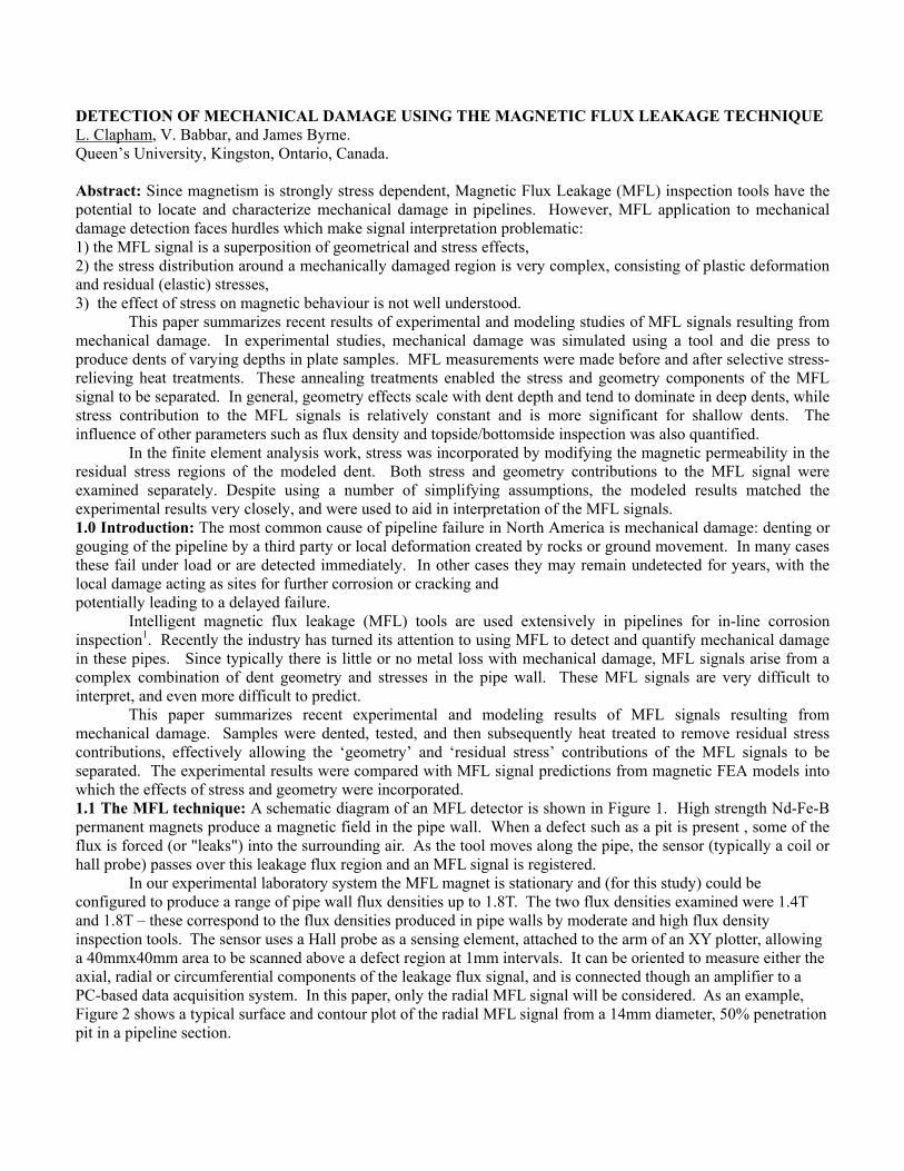
1.2 Sample preparation and testing: Samples of 0.12" (3mm) and 0.24” (6mm) thick plate were subjected to controlled denting using a compression testing machine. Prior to denting, the samples were stress relieved at 500oC for three hours to remove any pre-existing residual stresses. Dents were produced using a cylindrical tool with a rounded tip, which was pushed into the plate. A die containing a larger hole was located below the tool. Dents of two different diameters were produced. For ease of reference these were termed ‘small’ and ‘large’ dents, defined as below: Small dents: A 20mm diameter cylindrical tool was used to produce these dents in 0.12” (3mm) thick plate samples. Dents from 0.02" to 0.12" (0.5mm deep to 3mm deep) were produced, with varying diameters from 0.14" to 0.43" (3.5mm to 11mm). Large dents: A 40 mm diameter cylindrical tool was used to produce dents of approximately 1-1.5” diameter (25-36mm) in the 0.24” (6mm) plate samples. Dent depths ranged from 0.12” – 0.35” (3 – 8mm). 1.3 Heat treatments: Our earlier work [2] showed that the effect of residual stress on MFL signals can be removed using ‘traditional’ stress-relieving heat treatments. Therefore, in the present study, annealing was used to remove residual stress effects on the MFL signal, leaving only the MFL geometry component. 2.0 Results: After denting, MFL measurements were made on both sides of the dented sample. The concave side, termed the ‘topside’ of the sample, was the easiest side to measure – a thin sheet of plastic is placed over the ‘hole’ after which the hall probe moves essentially on a flat plane. The convex side, termed the ‘bottomside’ was more difficult to measure since the sensor must follow the dent contour. The bottomside results are of greater practical interest, however, since this is the side accessed in a typical pipeline inspection scenario. A full set of measurements were taken for both topside and bottomside orientations. For the sake of brevity, however, in the present paper we will focus primarily on the bottomside results, since these are most industrially relevant. Finally, in these bottomside measurements the sensor was fixed to always be parallel to the original plane of the sample (rather than the dent profile) as it traveled over the dent. 2.1 Small dents: bottomside MFL contour plots, before and after annealing: Figure 3 shows MFL signal contour plots (radial component) for small dents from 1.0mm deep up to 3mm deep (0.5mm was also tested but is essentially similar to the 1mm deep signal). MFL signals are shown prior to and after stress-relief annealing, for a flux density of 1.8T. Before annealing, (Figure 3 – Preanneal) MFL signals exhibit the following features: 1) a centre peak region which, for shallow dents, is similar to that seen for a typical corrosion pit (see Figure 2) and 2) four ‘shoulder peaks’ at approximately 45o to the applied field direction.

As the dents become deeper another fairly broad central peak develops between the two shoulder peaks – giving the appearance that the shoulder peaks are ‘growing together’.

After stress relief annealing (Figure 3 – post anneal) the most important result is that the ‘shoulder’ peaks essentially disappear, except in the deepest dent cases where some vestige of the shoulder peak signals still remain. Conversely, the centre peaks remain, as do the broad central peaks that formed between the shoulder peaks as the dents become deeper. Although the form of these centre peaks does not change, analysis of their heights indicate that they are slightly lower than before annealing. 2.2 Large dents: bottomside MFL contour plots, before and after annealing, B=1.8T: Figure 4 shows MFL signal contour plots (radial component) for the large dent samples, with dents from 3mm to 8mm depths. In comparison with the small dent results of Figure 3, the deeper dent signals display similar features but are generally larger in scale as expected. As with the smaller dents, the central peaks remains largely unaffected by annealing, while the shoulder peaks disappear or shrink considerably. Both the small (Fig 3) and large (Fig 4) dent results exhibit similar patterns before and after annealing. We are able to conclude from these results that the central MFL peaks are largely due to the dent geometry, although these peaks experience a size reduction with annealing which suggests a small stress contribution. The shoulder peaks, however, appear to be almost entirely stress-related, since they are diminished significantly, and often completely, during stress-relief annealing.

2.3 Comparison of topside and bottomside MFL contour plots: Figure 5 shows a example comparison of topside MFL versus bottomside MFL signal contour plots. Results are for large dents, 5.0mm deep, both pre and post-anneal. The background flux density is B=1.8T. Interestingly, there is little difference between the results, except in overall signal magnitude. All other dent geometries exhibited the same similarities between topside and bottomside MFL signals.

Figure 5. Comparison of MFL radial signals from the topside (top) and bottomside (bottom) of the dented sample,

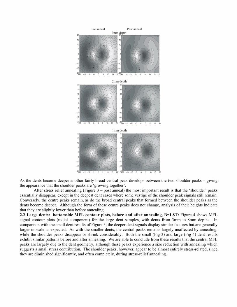
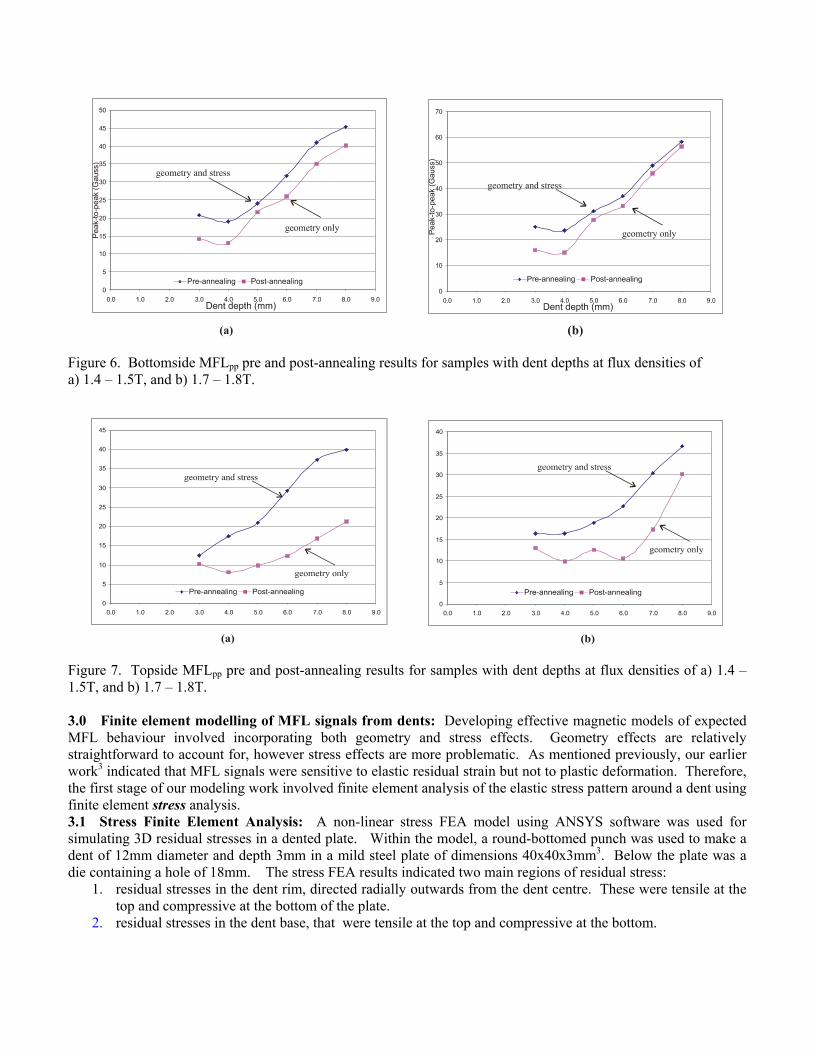
both before and after annealing. 2.4 MFL peak-to-peak comparisons: The MFLpp signal was also measured for all samples, however this only reflected the size of the main centre peak (a further study of the shoulder peak height is currently underway). Figure 6 and Figure 7 show bottomside and topside MFLpp results respectively, for the large dent samples. In both figures, (a) represents the low flux density results and (b) the high flux density case. The two sets of data on each graph indicate 1) the pre-annealing state where the MFL signal is comprised of both geometry and stress contributions, and 2) the post annealing state where the signal is predominately geometry induced. Overall, these plots indicate that the magnitude of the bottomside signals (Fig 6) tends to generally be higher than those of the topside (Figure 7), particularly at higher flux densities (figs 6(b) and 7(b)). Furthermore, the topside signals tend to be more significantly affected by stress, since the ‘gap’ between the topside curves is greater than that for the bottomside MFL. Finally, comparing flux density affects, the stress contribution to the MFL signal is at low flux densities (Figure 6(a) and Figure 7(a)) tends to be generally higher than at high flux densities.

Overall, these plots indicate that the magnitude of the bottomside signals (Fig 6) tends to generally be higher than those of the topside (Figure 7), particularly at higher flux densities (figs 6(b) and 7(b)). Furthermore, the topside signals tend to be more significantly affected by stress, since the ‘gap’ between the topside curves is greater than that for the bottomside MFL. Finally, comparing flux density affects, the stress contribution to the MFL signal is at low flux densities (Figure 6(a) and Figure 7(a)) tends to be generally higher than at high flux densities.

Figure 6. Bottomside MFLpp pre and post-annealing results for samples with dent depths at flux densities of a) 1.4 – 1.5T, and b) 1.7 – 1.8T.

Figure 7. Topside MFLpp pre and post-annealing results for samples with dent depths at flux densities of a) 1.4 – 1.5T, and b) 1.7 – 1.8T. 3.0 Finite element modelling of MFL signals from dents: Developing effective magnetic models of expected MFL behaviour involved incorporating both geometry and stress effects. Geometry effects are relatively straightforward to account for, however stress effects are more problematic. As mentioned previously, our earlier work3 indicated that MFL signals were sensitive to elastic residual strain but not to plastic deformation. Therefore, the first stage of our modeling work involved finite element analysis of the elastic stress pattern around a dent using finite element stress analysis. 3.1 Stress Finite Element Analysis: A non-linear stress FEA model using ANSYS software was used for simulating 3D residual stresses in a dented plate. Within the model, a round-bottomed punch was used to make a dent of 12mm diameter and depth 3mm in a mild steel plate of dimensions 40x40x3mm3. Below the plate was a die containing a hole of 18mm. The stress FEA results indicated two main regions of residual stress:

1. residual stresses in the dent rim, directed radially outwards from the dent centre. These were tensile at the top and compressive at the bottom of the plate.

2. residual stresses in the dent base, that were tensile at the top and compressive at the bottom.

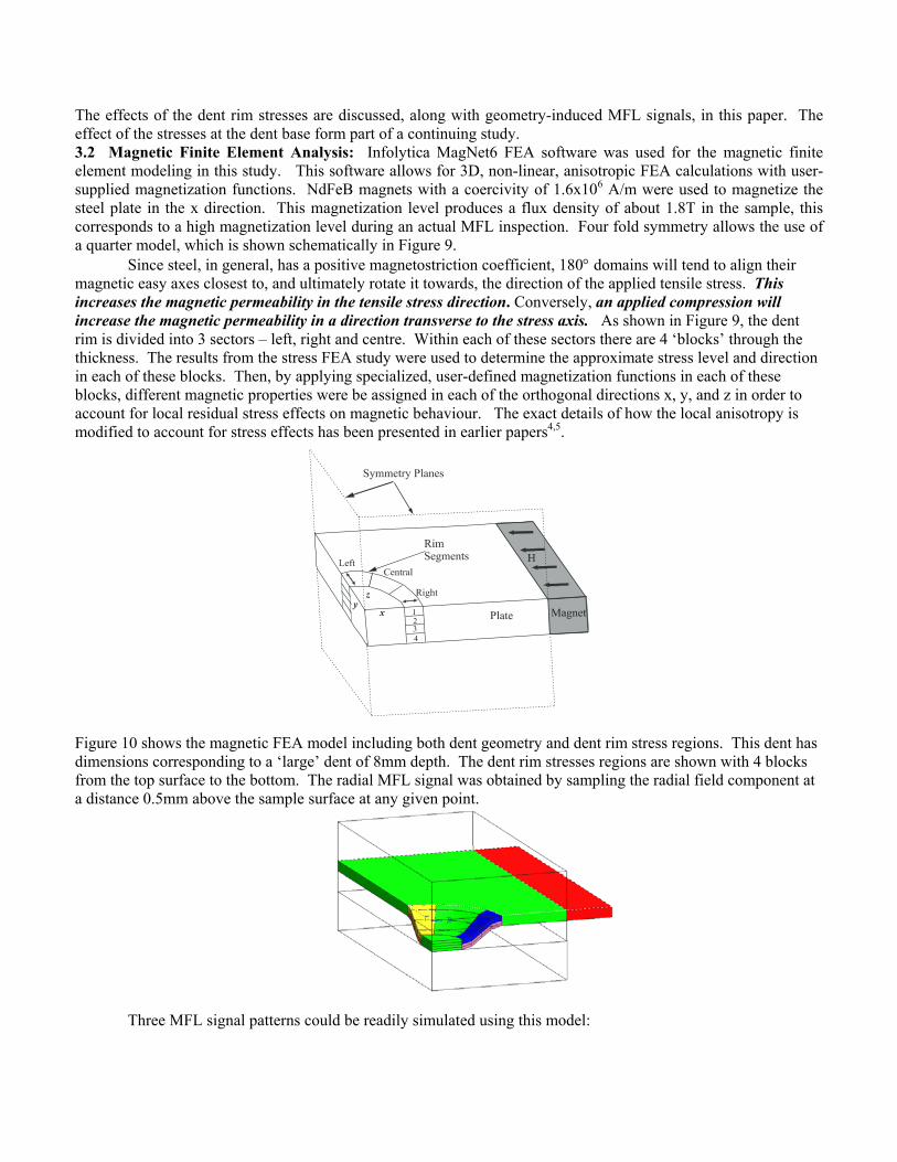
The effects of the dent rim stresses are discussed, along with geometry-induced MFL signals, in this paper. The effect of the stresses at the dent base form part of a continuing study. 3.2 Magnetic Finite Element Analysis: Infolytica MagNet6 FEA software was used for the magnetic finite element modeling in this study. This software allows for 3D, non-linear, anisotropic FEA calculations with user-supplied magnetization functions. NdFeB magnets with a coercivity of 1.6x106 A/m were used to magnetize the steel plate in the x direction. This magnetization level produces a flux density of about 1.8T in the sample, this corresponds to a high magnetization level during an actual MFL inspection. Four fold symmetry allows the use of a quarter model, which is shown schematically in Figure 9.

Since steel, in general, has a positive magnetostriction coefficient, 180° domains will tend to align their magnetic easy axes closest to, and ultimately rotate it towards, the direction of the applied tensile stress. This increases the magnetic permeability in the tensile stress direction. Conversely, an applied compression will increase the magnetic permeability in a direction transverse to the stress axis. As shown in Figure 9, the dent rim is divided into 3 sectors – left, right and centre. Within each of these sectors there are 4 ‘blocks’ through the thickness. The results from the stress FEA study were used to determine the approximate stress level and direction in each of these blocks. Then, by applying specialized, user-defined magnetization functions in each of these blocks, different magnetic properties were be assigned in each of the orthogonal directions x, y, and z in order to account for local residual stress effects on magnetic behaviour. The exact details of how the local anisotropy is modified to account for stress effects has been presented in earlier papers4,5.

Figure 10 shows the magnetic FEA model including both dent geometry and dent rim stress regions. This dent has dimensions corresponding to a ‘large’ dent of 8mm depth. The dent rim stresses regions are shown with 4 blocks from the top surface to the bottom. The radial MFL signal was obtained by sampling the radial field component at a distance 0.5mm above the sample surface at any given point.

Three MFL signal patterns could be readily simulated using this model:

1) dent geometry-only MFL signal: in this case all sample regions (dent and background plate) had isotropic magnetic parameters. 2) dent geometry + dent stress MFL signal: for this case all regions of the plate were isotropic except for the right and left dent rim region blocks, which were assigned anisotropic magnetic parameters corresponding to high tension or compression according to the results of the stress FEA modelling. Specifically, blocks in the ‘right’ region (Figure 9) had a strong x-direction anisotropy, tensile at the top and compressive at the bottom. Blocks in the ‘left’ region had a strong y-direction anisotropy, again tensile at the top and compressive at the bottom. Unfortunately, at this point it was not possible to account directly for shear- direction stresses in the central dent rim region, although some qualitative work was done on the influence that these might have. 3) dent stress-only signal: this MFL signal was generated by subtracting the ‘geometry-only’ signal from the geometry+stress signal. Figure 11 (a) and (b) below show the bottomside, geometry-only MFL signal and stress-only MFL signal for the modelled 8mm deep dent. In comparing Figure 11(a) with the experimental ‘geometry-only’ result for the 8mm deep large dent ( Figure 4, 8mm deep dent, post-anneal), an excellent correlation is observed. Figure 11(b) indicates that the dent rim stresses lead to a distinctive shoulder peak in the signal. In comparing this with the experimental results, we believe that this corresponds to the ‘stress shoulder peaks’ seen in pre-annealing MFL signals (see, for example Figure 4, pre-anneal, 3mm deep dent MFL signal).

In summary, this study has made a valuable contribution to the understanding of MFL generated from dents, effectively separating the stress and geometry contributions to the signal. Furthermore, the experimental work has validated the magnetic FEA modeling, despite current model limitations. References: 1. Clapham, L. and Atherton, D.L., 1999, "Magnetic Flux Leakage Inspection of Oil and Gas Pipelines" Proceedings of the Canadian Institute of Metallurgists Conference, Calgary, Canada. 2. L. Clapham, C. Heald, T. Krause and D.L. Atherton, 1999, "The Origin of a Magnetic Easy Axis in Pipeline Steels", J. Applied Physics, 86, 1574-1580. 3. C.-G. Stefanita, L. Clapham and D.L. Atherton, “Plastic vs Elastic Stress effects on Magnetic Barkhausen Noise” 2000, Acta Materialia, 48, 3545-3551. 4. F. Liorzou and D.L. Atherton, 1999, “Effects of compressive stress on a steel cube using tensor magnetization and magnetostriction analysis” J. Magnetism and magnetic materials, Vol. 195, 174-181. 5. V. Babbar, B. Shiari and L. Clapham, "Mechanical Damage Detection using Magnetic Flux Leakage Tools: Modelling the Effect of Localized Residual Stresses", 2004, IEEE Transaction on Magnetics, V40, 43-49.