8 Detection of the Greenhouse Effect in the Observations T.M.L. WIGLEY, T.P. BARNETT Contributors: T.L. Bell; P. Bloomfield; D. Brillinger; W. Degefu; C.K. Folland; S. Gadgil; G.S. Golitsyn; J.E. Hansen; K. Hasselmann; Y. Hayashi; P.D. Jones; DJ. Karoly; R.W. Katz; M.C. MacCracken; R.L. Madden; S. Manabe; J.F.B. Mitchell; A.D. Moura; C. Nobre; L.J. Ogallo; E.O. Oladipo; D.E. Parker; A.B. Pittock; S.C.B. Raper; B.D. Santer; M.E. Schlesinger; C.-D. Schonwiese; C.J.E. Schuurmans; A. Solow; K.E. Trenberth; K.Ya. Vinnikov; W.M. Washington; T. Yasunari; D. Ye; W. Zwiers.
Transcript
8
Detection of the Greenhouse Effect in the Observations
T.M.L. WIGLEY, T.P. BARNETT
Contributors: T.L. Bell; P. Bloomfield; D. Brillinger; W. Degefu; C.K. Folland; S. Gadgil; G.S. Golitsyn; J.E. Hansen; K. Hasselmann; Y. Hayashi; P.D. Jones; DJ. Karoly; R.W. Katz; M.C. MacCracken; R.L. Madden; S. Manabe; J.F.B. Mitchell; A.D. Moura; C. Nobre; L.J. Ogallo; E.O. Oladipo; D.E. Parker; A.B. Pittock; S.C.B. Raper; B.D. Santer; M.E. Schlesinger; C.-D. Schonwiese; C.J.E. Schuurmans; A. Solow; K.E. Trenberth; K.Ya. Vinnikov; W.M. Washington; T. Yasunari; D. Ye; W. Zwiers.
CONTENTS
Executive Summary 243
8.1 Introduction 245 8.1.1 The Issue 245 8.1.2 The Meaning of "Detection" 245 8.1.3 Consistency of the Observed Global-Mean
Warming with the Greenhouse Hypothesis 245 8.1.4 Attribution and the Fingerprint Method 247
8.3 Multivariate or Fingerprint Methods 252 8.3.1 Conspectus 252 8.3.2 Comparing Changes in Means and Variances 252
8.3.3 Pattern Correlation Methods 252
8.4 When Will the Greenhouse Effect be Detected ? 253
8.5 Conclusions 254
References 254
EXECUTIVE SUMMARY
Global-mean temperature has increased by 0 3-0 6°C over the past
100 years The magnitude of this warming is broadly consistent
with the theoretical predictions of climate models, but it remains
to be established that the observed warming (or part of it) can be
attributed to the enhanced greenhouse effect This is the detection
issue
If the sole cause ol the warming were the Man-induced
greenhouse effect, then the implied climate sensitivity would be
near the lower end of the accepted range of model predictions
Natural variability ot the climate system could be as large as the
changes observed to date but there are insufficient data to be able
to estimate its magnitude or its sign If a significant traction of
the observed warming were due to natural variability, then the
implied climate sensitivity would be even lower than model
predictions However it is possible that a larger greenhouse
warming has been offset paitially by natural variability and other
factors, in which case the climate sensitivity could be at the high
end of model predictions
Global-mean temperature alone is an inadequate indicator ot
greenhouse-gas-induced climatic change Identifying the causes
of any global-mean temperature change requires examination of
other aspects of the changing climate, particularly its spatial and
temporal characteristics Currently, there is only limited
agreement between model predictions and observations Reasons
for this include the fact that climate models are still in an early
stage of development, our inadequate knowledge of natural
variability and other possible anthropogenic effects on climate,
and the scarcity of suitable observational data, particularly long,
reliable time series An equally important problem is that the
appropriate experiments, in which a realistic model of the global
climate system is forced with the known past history of
greenhouse gas concentration changes, have not yet been
performed
Improved prospects for detection requne a long tenn
commitment to comprehensively monitoring the global climate
system and potential climate forcing factors and to reducing
model uncertainties In addition there is consideiable scope lor
the refinement of the statistical methods used for detection We
therefore recommend that a compiehensive detection strategy be
lomiulated and implemented in order to improve the prospects lor
detection This could be facilitated by the setting up ol a fully
integrated international climate change detection panel to
coordinate model experiments and data collection eltorts directed
towards the detection problem
Quantitative detection of the enhanced greenhouse effect using
objective means is a vital research area, because it is closely
linked to the reduction of uncertainties in the magnitude of the
effect and will lead to increased confidence in model projections
The fact that we are unable to reliably detect the predicted signals
today does not mean that the greenhouse theory is wiong or that
it will not be a serious problem for mankind in the decades ahead
8 Detection of the Gi eenhouse Ejfee t in the Obsei \ ations 24^
8.1 Introduction
8.1.1 The Issue This chapter addresses the question Have we detected the greenhouse effect' , or, stated more correctly, have we detected changes in climate that can, with high statistical confidence, be attributed to the enhanced greenhouse effect associated with increasing trace gas concentrations9 It is important to answer this question, because detecting the enhanced greenhouse effect will provide direct validation of models of the global climate system Until we can identify aspects of greenhouse gas induced changes in the observed climate record with high confidence, there will always be doubts about model validity and hence about even the most general predictions of future climatic change Even when detection has occurred uncertainties regarding the magnitude and spatial details of futuie changes will still remain
Previous reviews of the greenhouse problem (N R C 1983, MacCracken and Luther, 1985 Bolin et al 1986) have also addressed the detection issue They have concluded that the enhanced greenhouse effect has not yet been detected unequivocally in the observational record However, they have also noted that the global mean temperature change over the past 100 years is consistent with the greenhouse hypothesis, and that theie is no convincing observational evidence to suggest that the model-based range of possible climate sensitivity ' values is wrong The purpose ol the present review is to re evaluate these conclusions in the light of more recent evidence
8.1.2 The Meaning Of "Detection " The word "detection has been used to leler to the identification of a significant change in climate (such as an upward trend in global mean temperature) However identifying a change in climate is not enough for us to claim that we have detected the enhanced gi eenhouse effect, even if statistical methods suggest that the change is statistically significant (I e extremely unlikely to have occurred by chance) To claim detection in a useful and practical way, we must not only identify a climatic change, but we must attribute at least part of such a change to the enhanced greenhouse effect It is in this stricter sense that the word "detection is used here Detection requires that the observed changes in climate are in accord with detailed model predictions of the enhanced greenhouse effect, demonstrating that we understand the cause or causes of the changes
1 Climate sensiti\ it\ is defined heie as the eqmlibi nun global-mean tempeiatme change foi a CO2 doubling (AT2\) &T2\ ls thought to he in the tanqe 1 5°C to 4 5°C (see Section 5)
To illustrate this important dilterence consider changes in global-mean temperature A number ol recent analyses have claimed to show a statistically significant warminj. trend over the past 100 years (Hansen et al 1988 Tsionis and Eisner, 1989, Wigley and Raper 1990) But is this warming trend due to the enhanced greenhouse effect' We have strong evidence that changes of similar magnitude and rate have occurred prior to this century (see Section 7) Since these changes were certainly not due lo the enhanced greenhouse effect, it might be argued that the most ieccni changes merely represent a natuial long-time-scale fluctuation
The detection problem can be conveniently described in terms of the concepts of signal and noise (Madden and Ramanathan 1980) Here the signal is the predicted time dependent climate response to the enhanced greenhouse effect The noise is any climatic variation that is not due to the enhanced greenhouse effect : Detection requires that the observed signal is large relative to the noise In addition in order to be able to attribute the detected signal to the enhanced greenhouse effect it should be one that is specific to this particular cause Global mean warming foi example is not a particularly good signal in this sense because there are many possible causes of such warming
8.1.3 Consistency Of The Observed Global-Mean Warming With The Greenhouse Hypothesis
Global-mean temperature has incieased by around 0 3-0 6°C over the past 80-100 years (see Section 7) At the same time, greenhouse gas concentrations have inci eased substantially (Section 1) Is the warming consistent with these increases7 To answer this question we must model the effects of these concentration changes on global-mean temperature and compaie the results with the obseivations Because of computing constraints and because of the relative inflexibility of coupled ocean atmospheie GCMs we cannot use such models for this purpose Instead we must use an upwellmg-ditfusion climate model to account foi damping or lag efiect of the oceans (see Section 6) The response of such a model is deteimined mainly by the climate sensitivity (AT2\) the magnitude of ocean mixing (specified by a diffusion coefficient K) and the latio of the temperature change in the regions ol sinking watei relative to the global-mean change (JC) Uncertainties in these parameters can be accounted for by using a range of \alues
2 Noisi as used hen includes \anations that mn>hi be due to othei antluopoi>emc effects (see Section!) and natuial \anahilit\ Natuial \aiiabilit\ ufeistoall iiatuial c lunatic \ ai unions that aie uni c late cl to Man s actmtic s imbiacins> both the effects of c \tcinal fou mj factois (suchas soldi actmt\ and \ohanu ouptions) and mtc l nalh yenc i cited i at icibilits I ncci tannic s in the obse i \ ations also c onstitute a foi in of noise
246 Detec tion of the Gi eenhouse Effect in the Obsei \ at ions 8
tem
p ch
ange
(°C
) U
l o
c cc CD
E i
co O ^ 0 0 O
I
- K =
-
• i = 0.63,
~ Observed
i i i
i i i
7 T = 1
- ; $ 5 ^
I I I
I I I I I I
AT2x = Si
Modelled / A 3 /
—•-1860 1880 1900 1920 1940 1960 1980
Year 1860 1880 1900 1920 i g V ^ o 19 '80
Year
1860 1880 1900 1920 1940 1960 1980
Year 1860 1880 1900 1920 1940 1960 1980
Year
Figure 8.1: Observed global-mean tcmpcrutuie changes (1861 1989) compaied with predicted values The observed changes are as given in Section 7 smoothed to show the decadal and longer time scale trends more cleaily Predictions are based on observed concentiation changes and concentiaiion/forcing lelationships given in Section 2 and have been calculated using the upwelhng diffusion climate model of Wigley and Raper (1987) To provide a common ieteience level modelled and observed data have been adjusted to have zero mean over 1861 1900 To illustrate the sensitivity to model parameters model results are shown for AT2X = 1,' 3 4 and VC (all panels) and for four K, 7t combinations The top left panel uses the values recommended in Section 6 (K = 0 6^cm2sec ', 71 =1) Since sensitivity to K is relatively small and sensitivity to 71 is small for small AT2X. the best fit AT2X depends little on the choice of K and 71
The model is forced from 176S-1990 using concentration consistent with the observations on the century time-scale
changes and radiative forcing/concentration relationships Agreement on long time-scales is about all that one might
given in Section 2 expect On shorter time-scales, we know that the climate
Figure 8 1 compares model predictions foi various system is subject to internal variability and to a variety of
model parameter values with the observed warming ovei external forcings, which must obscure any response to
1861-1989 The model results are clearly qualitatively greenhouse forcing Although we cannot explain the
8 Detec turn of the Gieenliouse Effec t in the Ohsei \ations 247
observed shorter time-scale lluctuations in detail, their
magnitude is compatible with our undei standing ol natural
climatic variability Essentially, they reflect the noise
against which the greenhouse signal has to be detected
While the decadal time-scale noise is clear, there may
also be substantial century time-scale noise This noise
makes it difficult to inter a value of the climate sensitivity
from Figure 8 1 Internal variability arising iiom the
modulation of random atmospheric disturbances by the
ocean (Hasselmann, 1976) may produce warming or
cooling trends of up to 0 3°C per century (Wigley and
Raper, 1990, see Figure 8 2), while ocean circulation
changes and the effects of other external forcing factors
such as volcanic eruptions and solar irradiance changes
- STOUFFERE7 4Z.
+0 2
—02
WIGLEY&RAPER
Figure 8.2: Simulated natural variability ot global mean temperature The upper panel shows results from the 100 year control run with the coupled ocean/atmosphere GCM ot Stoutter et al (1989) These data are also shown in Figure 6 2 The lower two panels are 100 year sections from a 100 000 year simulation using the upwelling-diffusion model employed in Figure 8 1 with the same climate sensitivity as the Stouffer et al model (ATTX = 4°C) The upwellmg diffusion model is forced with random inter annual radiative changes chosen to match observed inter annual variations in global-mean temperature (Wigley and Raper 1990) The consequent low frequency variability arises due to the modulating effect of oceanic thermal inertia Most 100 yeai sections are similar in chaiactei to the middle panel and are qualitatively indistinguishable from the coupled ocean/atmospheie GCM results However a significant fraction show century time scale trends as huge oi laigei than that in the lower panel Longer GCM simulations may therefore icveal similar centuiy time scale vai lability
and/or other anthropogenic factors (sec Section 2) could
produce trends of similar magnitude On time-scales ol
order a decade, some of these (volcanic eruptions sulphate
aerosol derived cloud albedo changes) clearly have a
negative forcing effect, while others have uncertain sign II
the net century time-scale effect of all these non
greenhouse factors were close to zero, the climate
sensitivity value implied by Figure 8 1 would be in the
range 1 °C to 2°C If their combined effect were a warming
then the implied sensitivity would be less than 1°C, while it
it were a cooling the implied sensitivity could be largei
than 4°C The range of uncertainty in the value of the
sensitivity becomes even larger if uncertainties in the
observed data (Section 7) are accounted for
From this discussion, one may conclude that an
enhanced greenhouse effect could already be present in the
climate record, even though it cannot yet be reliably
detected above the noise of natural climatic vai lability The
goal of any detection strategy must be to achieve much
more than this It must seek to establish the credibility ol
the models within relatively narrow limits and to reduce
our uncertainty in the value of the climate sensitivity
parameter In this regard, global-mean temperature alone is
an inadequate indicator of greenhouse gas induced climatic
change Identifying the causes of any global-mean
temperature change requires examination of other aspects
of the changing climate, particularly its spatial and
temporal characteristics
8.1.4 Attribution And The Fingerprint Method
Given our rudimentary understanding of the magnitude and
causes of low-frequency natural variability it is virtually
impossible to demonstrate a cause-effect ielationship with
high confidence from studies of a single variable
(However, if the global warming becomes sufficiently
large, we will eventually be able to claim detection simply
because there will be no other possible explanation)
Linking cause and effect is refeired to as attribution
This is the key issue in detection studies - we must be able
to attribute the observed changes (or part ot them) to the
enhanced greenhouse effect Confidence in the attribution
is increased as predictions of changes in various
components of the climate system aie borne out by the
observed data in more and more detail The method
proposed for this purpose is the fingerprint method
namely, identification of an observed multivariate signal '
that has a structure unique to the predicted enhanced
greenhouse effect (Madden and Ramanathan 1980 Baker
and Barnett, 1982, MacCracken and Moses 1982) The
1 A multnaiuite signal could he change s //; a sini>k c lunate element (sue h a s tempo atui c) at man \ plac c\ <n le\els in the atmosphei e oi changes in a numhci of diffeient elements oi changes in diffaint elements at different places
248 Dctec tion of the Gieenhouse Effec t in the Ohsei \ations 8
current scientific focus in the detection issue is thereloic on multivariate or fingerprint analyses The fingerprint method is essentially a form of model validation, wheie the perturbation experiment that is being used to test the models is the currently uncontrolled emission of greenhouse gases into the atmosphere The method is discussed further in Section 8 3 First, however, we consider some of the more general issues of a detection strategy
8.2 Detection Strategies
8.2.1 Choosing Detection Variables There are many possible climate elements or sets of elements that we could study to try to detect an enhanced greenhouse effect In choosing the ones to study, the following issues must be considered
the strength of the predicted signal and the ease with which it may be distinguished from the noise,
uncertainties in both the predicted signal and the noise, and
the availability and quality of suitable observed data
8 2 11 Signal to noise tatios The signal-to-noise ratio provides a convenient criterion for ranking different possible detection variables The stronger the predicted signal relative to the noise, the better the variable will be for detection purposes, all other things being equal For multivariate signals, those for which the pattern of natural variability is distinctly different from the pattern of the predicted signal will automatically have a high signal-to noise ratio
Signal to-noise ratios have been calculated tor a number of individual climate elements from the results of lxCCb and 2xCC>2 equilibrium experiments using atmospheric GCMs coupled to mixed-layei oceans (Bainett and Schlesinger 1987, Santer et al , 1990 Schlesinger ct al 1990) The highest values were obtained lor free troposphere temperatures, near-surface tempeiatures (including sea-surface temperatures), and lower to middle troposphenc water vapour content (especially in tropical regions) Lowest values were iound for mean sea level pressure and precipitation While these results may be model dependent, they do provide a useful preliminary indicator of the relative values of different elements in the detection context
Variables with distinctly difleient signal and noise patterns may be difficult to find (Bamett and Schlesinger, 1987) There are reasons to expect parallels between the signal and the low-frequency noise patterns at least at the zonal and seasonal levels, simply because such char actenstics anse through feedback mechanisms that are common to both greenhouse forcing and natural variability
82 I 2 Signal umeitauities Clearly a vanable toi which the signal is highly uncertain cannot be a good candidate as a detection variable Predicted signals depend on the models used to produce them Model-to-model differences (Section 5) point strongly to laige signal uncertainties Some insights into these uncertainties may also be gained from studies ol model results in attempting to simulate the present-day climate (see Section 4) A poor representation of the present climate would indicate greater uncertainty in the predicted signal (e g , Mitchell et al , 1987) Such uncertainties tend to be largest at the regional scale because the processes that act on these scales are not accurately represented or paiametenzed in the models Even if a particular model is able to simulate the present-day climate well, it will still be difficult to estimate how well it can define an enhanced greenhouse signal Nevertheless, validations of simulations ol the present global climate should form at least one of the bases for the selection of detection variables
A source of unccitainty hcie is the difference between the results of equilibrium and transient experiments (see Section 6) Studies using coupled ocean-atmosphere GCMs and time-varying CO2 loicing have shown reduced warming in the aieas of deep water formation (1 e , the North Atlantic basin and around Antarctica) compared with equilibrium results (Bryan ct al , 1988, Washington and Mcehl, 1989, Stouffer et al , 1989) These experiments suggest that the regional patterns of temperature change may be more complex than those predicted by equilibrium simulations The results of equilibrium experiments must therefore be considered as only a guide to possible signal structuie
The most reliable signals aie likely to be those related to the largest spatial scales Small-scale details may be eliminated by spatial averaging, or, more generally by using filters that pass only the larger scale (low wave number) components (Note that some relatively small-scale features may be appropriate for detection purposes, if model confidence is high ) An additional benefit of spatial averaging or filtenng is that it results in data compression (1 e , reducing the dimensionality of the detection variable), which facilitates statistical testing Data compression may also be achieved by using linear combinations of variables (e g , Bell, 1982, 1986, Kaioly, 1987, 1989)
8 2 13 Noise unteitamties Since the expected man-made climatic changes occur on decadal and longer time-scales, it is largely the low-frequency characteristics of natural variability that are important in defining the noise Estimating the magnitude of low frequency variability presents a major problem because of the shoitness and incompleteness of most
8 Detec Hon of the Gi eenhouse Effcc t in the Obsei \ atiom 249
instrumental records This problem applies particularly to new satellite-based data sets
In the absence ol long data senes, statistical methods may be used to estimate the low frequency variability (Madden and Ramanathan, 1980, Wigley and Jones, 1981), but these methods depend on assumptions which introduce their own uncertainties (Thiebaux and Zwiers, 1984) The difficulty arises because most climatological time-series show considerable persistence, in that successive yearly values are not independent, but often significantly correlated Serially correlated data show enhanced low frequency variability which can be difficult to quantily
As an alternative to statistically-based estimates, model simulations may be used to estimate the low-frequency variability, either for single variables such as global-mean temperature (Robock, 1978, Hansen et al , 1988, Wigley and Raper, 1990) or lor the full three-dimensional character of the climate system (using long simulations with coupled ocean-atmosphere GCMs such as that of Stouller et al , 1989) Internally-generated changes in global-mean temperature based on model simulations are shown in Figure 8 2
82 14 Obsei\eddata a\ailabiht\ The final, but certainly not the least important factor in choosing detection variables is data availability This is a severe constraint loi at least two reasons, the definition of an evolving signal and the quantification of the low-frequency noise Both iequire adequate spatial coverage and long record lengths, commodities that are rarely available Even for surlace vaiiables global scale data sets have only recently become available (see Section 7) Useful upper air data extend back only to the 1950s and extend above 50mb (i e , into the lowci stratosphere) only in recent years Comprehensive three-dimensional coverage of most variables has become available only recently with the assimilation ol satellite data into model-based analysis schemes Because such data sets are produced for meteorological purposes (e g model initialisation), not for climatic purposes such as long-term trend detection, they contain residual inhomogeneilies due to changes in instrumentation and liequent changes in the analysis schemes In short, we have very lew adequately observed data variables with which to conduct detection studies It is important therefore to ensure that existing data senes are continued and observational programmes are maintained in ways that ensure the homogeneity of meteorological records
8.2.2 Univariate Detection Methods A convenient way to classify detection studies carried out to date is in terms ol the number ol elements (oi vaiiables) considered, i e , as univariate or multivaiiate studies The key characteristic ol the foimei is that the detection
variable is a single time series Almost all published univariate studies have used tempeutuie averaged over a large area as the detection parametei A cential pioblem in such studies is defining the noise level I e , the low Irequency variability (see 8 2 13)
There have been a number of published variations on the univariate detection theme One such has been iclened to as the noise reduction method In this method theeflectsol other external forcing lactors such as volcanic activity and/or solar irradiance changes or internal factors such as ENSO are removed from the record in some deteimmistic (i e , model-based) or statistical way (Hansen et al 1981 Gilhland 1982 Vinmkov and Groisman 1982 Gilhland and Schneider. 1984 Schonwiese 1990) This method is fraught with uncertainty because the history ol past forcings is not well known Theic are no dncct observations of these forcing factois and they have been inferred in a variety of different ways leading to a number of different forcing histones (Wigley et al 1985 Schonwiese, 1990) The noise reduction pnnciple however, is important Continued monitoring ol any ol the factors that might influence global climate in a deterministic way (solar irradiance, stratospheric and troposphenc aerosol concentrations, etc ) can make a significant contribution to facilitating detection in the future
As noted above in the case of global-mean temperature univariate detection methods suffer because they consider change in only one aspect of the climate system Change in a single element could result from a variety of causes making it difficult to attribute such a change specilically to the enhanced greenhouse effect Nevertheless it is useful to review recent changes in a number ol variables in the light of current model piedictions (see also Wood 1990)
8.2.3 Evaluation Of Recent Climate Changes 8 2 3 1 Int i ease of global mean tempt i alia c The primary response ol the climate system to mcieasing greenhouse gas concentrations is expected to be a global-mean waiming of the lower layers ol the atmospheic In Section 8 13 the observed global mean wanning ol 0 3-0 6°C ovei the past century or so was compared with model predictions It was noted that the obscived wanning is compatible with the enhanced greenhouse hypothesis but that we could not claim to have detected the gieenhousc effect on this basis alone It was also noted that the dnectly implied climate sensitivity (i e the value of Al2\) was at the low end ol the expected range, but that the plethora ol uncertainties surrounding an empirical estimation ol AT?\ piecludes us drawing any lirm quantitatisc conclusions The observed global warming is tar liom being a steady monotonic upward trend but this does not mean that we should ie)cct the gieenhouse hypothesis Indeed although oui understanding ol natural climatic \ailability is siill
250 Detec turn of the Gieenhouse Effec t in the Obsei \ations 8
quite limited, one would certainly expect substantial natural fluctuations to be superimposed on any greenhouse-related warming trend
82 3 2 Enhanced hn>h-Iatitude waimms, paituulaih in the u intei half-yeai
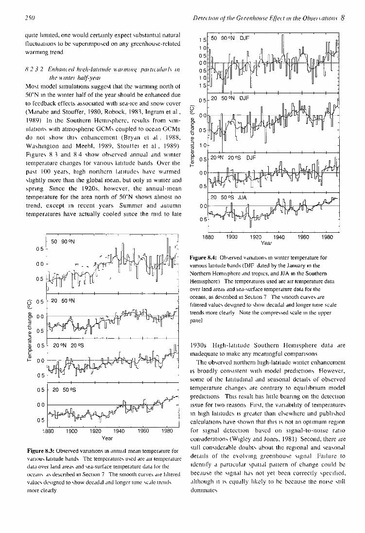
Most model simulations suggest that the warming north of 50°N in the winter half of the year should be enhanced due to feedback effects associated with sea-ice and snow cover (Manabe and Stouffer, 1980, Robock, 1983, Ingram et al , 1989) In the Southern Hemisphere, results from simulations with atmospheric GCMs coupled to ocean GCMs do not show this enhancement (Bryan et al , 1988, Washington and Meehl, 1989, Stoutlei et al , 1989) Figures 8 3 and 8 4 show observed annual and winter temperature changes for various latitude bands Over the past 100 years, high northern latitudes have warmed slightly more than the global mean, but only in winter and spring Since the 1920s, however, the annual-mean temperature for the area north of 50°N shows almost no trend, except in recent years Summer and autumn temperatures have actually cooled since the mid to late
1880 1900 1920 1940 Year
1960 1980
Figure 8.3: Observed variations in annual mean temperature for various latitude bands The temperatures used are air temperature data over land areas and sea-surface temperature data tor the oceans as described in Section 7 The smooth curves aie liltered values designed to show decadal and longer time scale trends more clearly
O
U)
a. E
1880 1900 1920 1940 Year
1960 1980
Figure 8.4: Observed variations in winter temperature for various latitude bands (DJF dated by the January in the Northern Hemisphere and tropics, and JJA in the Southern Hemisphere) The temperatures used are air temperature data over land areas and sea-surface temperature data for the oceans, as described in Section 7 The smooth curves are filtered values designed to show decadal and longer time scale trends more clearly Note the compressed scale in the upper panel
1930s High-latitude Southern Hemisphere data are inadequate to make any meaningful comparisons
The observed northern high-latitude winter enhancement is broadly consistent with model predictions However, some of the latitudinal and seasonal details of observed temperature changes are contrary to equilibrium model predictions This result has little bearing on the detection issue for two reasons First, the variability of temperatures in high latitudes is greater than elsewhere and published calculations have shown that this is not an optimum region for signal detection based on signal-to-noise ratio considerations (Wigley and Jones, 1981) Second, there are still considerable doubts about the regional and seasonal details of the evolving greenhouse signal Failure to identify a particular spatial pattern of change could be because the signal has not yet been correctly specified, although it is equally likely to be because the noise still dominates
8 Detection of the Gi eenhouse Effect in the Obsenations 2SI
82 3 3 Tioposplwiic wainum> and \tiatospheiit toolim> All equilibrium model simulations show a wanning to near the top of the troposphere (Section 5) Trends near the tropopause and for the lowei stiatosphere, at least up to 50mb, differ in sign between models Above 50mb, all models show a cooling It has been suggested that this contrast in trends between the troposphere and stratospheie might provide a useful detection fingerprint (Epstein, 1982, Parker, 1985, Karoly 1987, 1989), but this is not necessarily the case lor a number of reasons First, identification of such a signal is hampered because observations above 50mb are of limited duration and generally of poorer quality than those in the troposphere Second, there arc reasons to expect natural variability to show a similar contrast between stratospheric and troposphenc trends (Liu and Schuurmans 1990)
Stratospheric cooling alone has been suggested as an important detection vanable, but its interpretation is difficult because it may be caused by a number ol other factors, including volcanic eiuptions and 07one depletion Furthermore, the physics of gieenhouse gas induced stratospheric cooling is much simplei than that of troposphenc wanning It is quite possible for models to behave correctly in then stiatosphenc simulations yet be seriously in error in the lower atmospheie Validation of the stratospheric component of a model while of scientific importance, may be of little relevance to the detection of an enhanced greenhouse eltect in the tioposphere
Nevertheless, there is broad agieement between the observations and equilibrium model simulations While the observations (Angell 1988) show a global-mean cooling tiend from 1958 between lOOhPa and ^OOhPa (Section 7, Figure 7 17), which appears to conflict with model results this cooling is apparent only between 10 and 10°N (where it is not statistically significant) and south of 60°S (wheic it is associated with the ozone hole) There are no noticeable trends in other regions Data compiled by Karoly (1987 1989) show a warming trend since 1964 up to aiound 200hPa in the Southern Hcmispheic to lOOhPa in the Northern Hemisphere to 60°N and a moie complex (but largely warming) behaviour north ol 60°N Near the tiopopause and in the lowci stiatosphere tempeiatuics have cooled since 1964 The main diffeience between recent observations and model simulations is in the level at which warming reverses to cooling Although the models show large model-to-model differences, this level is generally lower in the observations This diffeience may be associated with poor vertical resolution and the inadequate representation of the tiopopause in current climate models
8 2 14 Global-mean pi et ipitation mc i ease Equilibrium expenments with GCMs suggest an inciease
in global-mean precipitation as one might expect from the
associated increase in atmosphenc tempciattire However the spatial details of the changes aie highly unceilain (Schlesinger and Mitchell 1987, and Section 5) Observations liom which the long term change in precipitation can be determined are available only ovei land aieas (see Bradley et al , 1987, Did/ et al , 1989, and Section 7), and there are major data problems in teims of coverage and homogeneity These difficulties, coupled with the recognized model deficiencies in their simulations of precipitation and the likelihood that the precipitation signal-to-noise ratio is low (see 82 1 1), preclude any meaningful comparison
8 2 3 5 Sea le\ el 11 se Increasing greenhouse gas concentrations are expected to cause (and have caused) a rise in global-mean sea level due partly to oceanic thermal expansion and paitly to melting of land-based ice masses (see Section 9) Because of the strong dependence of sea level rise on global mean temperatuie change, this element, like global mean precipitation, cannot be considered as an independent variable Observdtions show that global-mean sea level has risen over the past 100 years, but the magnitude of the rise is uncertain by a factor of at ledst two (see Section 9) As fdr ds it cdn be judged, there hds been d positive thermdl expansion component of this sea level rise Observational evidence (e g , Meier, 1984, Wood, 1988) shows that there has been a general long term retreat of small glacicis (but with mdrked regional and shorter time-scale variability) and this process has no doubt contributed to sea level rise Both thermal expansion and the melting of small glaciers are consistent with global warming, but neither provides any independent information about the cause of the warming
82 3 6 Tiopospheiu watei \apow nun use Model predictions show an increase in tioposphenc water vapour content in association with mcieasing atmosphenc temperature This is ol consideiable impoitance since it is responsible for one ol the main feedback mechanisms that amplifies the enhanced greenhouse effect (Raval and Ramanalhan 1989) Furthermore, a model-based signal to noise ratio analysis (see Section 8 2 11) suggests that this may be a good detection variable Howevci the brevity of avdildble lecords and data inhoinogeneities preclude any conclusive assessment of trends The available data have inhomogeiieities due to major changes in radiosonde humidity instrumentation Since the mid 1970s iheic has been an apparent upward trend, largest in the tropics (Flohn and Kapala 1989 Elliott et al 1990) Howevci the magnitude of the tropical trend is much larger than anv expected gieenhouse-ielated change, and it is likely lhal natural vailability is dominating the recoid
252 Detec tion of the Gi eenhouse Effet t m the Obsei \ ationi 8
8.3 Multivariate or Fingerprint Methods
8.3.1 Conspectus The lingcrpnnt method, which involves the simultaneous use ol more than one time series, is the only way that the attribution problem is likely to be solved expeditiously In its most general form one might consider the time evolution ol a set of three-dimensional spatial fields, and compare model results (I e , the signal to be detected) with observations There are, however, many potential dill lculties both in applying the method and in interpreting the results, not the least of which is reliably defining the greenhouse-gas signal and showing a prion that it is unique
In studies that have been perlormed to date, predicted changes in the three-dimensional structure ol a single variable (mean values, variances and/or spatial patterns) have been compared with observed changes The com panson involves the testing ol a null hypothesis namely that the observed and modelled fields do not differ Rejection ol the null hypothesis can be interpreted in several ways It could mean that the model pattern was not present in the observations (1 e in simplistic tcims that there was no enhanced greenhouse el feet) or that the signal was obscured by natural variability or that the piediction was at fault in some way, due eithei to model eirois oi because the chosen prediction was inappropriate We know a prion that current models have numerous deficiencies (see Sections 4 and 5), and that even on a global scale, the piedicted signal is probably obscuied by noise (Section 8 I 1) Furthermore, most studies to date have only used the results ol equilibrium simulations lather than the more appropnate time-dependent results ol coupled ocean-atmosphcic GCM experiments 4 Because of these factors published woik in this area can onl\ be considered as exploiatory, dnected largely towaids testing the methods and investigating potential statistical problems
8.3.2 Comparing Changes In Means And Variances Means, time vanances and spatial variances ol the fields of observed and predicted changes have been compared loi a number of vanables by Sanlci ct al (1990) Predicted changes were estimated from the equilibrium lxCCb and 2xC02 simulations using the Oicgon State University (OSU) atmospheric GCM coupled to a mixed layer ocean (Schlesinger and Zhao, 1989) In all cases (different vanables, different months) the observed and modelled fields wcie found to be significantly different I e , for these
4 In this iei>aid the conect expeiinwnt simulation of changes to date in iespouse to obsened qieenhouse i>as fox mt>s has not \et been pei•foimed Because a i ealistic model simulation H ould t>eneiate its ow n substantial natuial i ai iabilit\ a numbei of sue h e\peiunents ma\ be lequucd in oulei to ensuie that iepic sentatne iesults aie obtained
tests the null hypothesis of no difference was rejected and the model signal could not be identified in the observations As noted above this is not an unexpected result
8.3.3 Pattern Correlation Methods The basic approach in pattern correlation is to compare the observed and modelled time-averaged patterns of change (or changing observed and modelled patterns) using a correlation coellicient or similar statistic The word "pattern is used in a very general sense - it may refer to a two point pattern involving two time series of the same vanable or to a many-point pattern involving the full three-dimensional spatial fields of more than one variable In some studies time-standaidi7ed variables have been used This has the advantage ol giving greater emphasis to those spatial legions in which the time variance (l e , the noise) is smallest
Four examples ol pattern correlation detection studies have appeared in the literature, all involving compansons of observed and modelled temperature changes (Barnett, 1986, Barnett and Schlesingei, 1987, Barnett, 1990, Santer et al , 1990) Barnett (1986) and Barnett and Schlesinger (1987) used the covariance between the patterns of standardized observed and modelled changes as a test statistic Equilibrium lxCO? and 2xCG"2 results from the OSU atmospheric GCM coupled to a mixed-layer ocean were employed to generate the multivariate predicted signal This pattern was then correlated with obseived changes ielative to a reference year on a year-by-year basis A significant trend in the correlation would indicate the existence of an increasing expression of the model signal in the observed data which could be interpreted as detection of an enhanced gieenhouse signal A marginally significant trend was appaient, but this was not judged to be a iobust result
Santei et al (1990) used the same model data and the spatial coi relation coelfluent between the time-averaged patterns ol obseived and piedicted change as a detection parameter The observed changes used were the differences between two decades 1947 % and 1977-86 Statistically significant dillciences between observed and model patterns ol temperature change were found in all months but February (for which the amount of common vanance was very small, less than 4%)
Barnett (1990) compared observed data with the time-evolving spatial fields from the GISS transient GCM run (Hansen et al , 1988) The model run uses realistic time-dependent forcing beginning in the year 1958, and accounts for the lag effect of oceanic thermal inertia by using a diffusion parameterization of heat transport below the mixed layer Comparisons were made using spatial correlation coefficients between decadal means ol the evolving signal and the equivalent pattern in the
8 Detec twn of the Gi eenhoust Ejjei t in the Ohsei \ attain 25?
observations Theie was virtually no similarity between modelled and obscived temperatuie patterns
The largely negative results obtained in these studies can be interpreted in a variety of ways as noted in Section 8 3 1 Because of this, failure to detect the model signal in the data cannot be taken as evidence that there is no greenhouse-gas signal in the real world Future multivariate detection studies should employ coupled ocean-atmosphere GCMs forced with obseived greenhouse-gas concentration changes over more than just the past few decades
8.4 When Will The Greenhouse Effect be Detected ?
The fact that we have not yet detected the enhanced greenhouse eflect leads to the question when is this likely to occur7 As noted earlier, detection is not a simple yes/no issue Rather it involves the gradual accumulation of evidence in suppoit of model predictions, which in parallel with improvements in the models themselves, will increase our confidence in them and progressively narrow the uncertainties regarding such key parameters as the climate sensitivity Unceitainties will always remain Predicting when a certain confidence level might be reached is as dilficult as predicting future climate change - moie so, in fact, since it requnes at least estimates of both the future signal and the futuie noise level
Nevertheless, we can provide some information on the time-scale for detection by using the unprecedented change concept mentioned buefly in Section 8 1 4 This should provide an upper bound to the time for detection since more sophisticated methods should pioduce earlier results We take a conservative view as a starting point namely that the magnitude of natuial variability is such that all of the warming of the past centuiy could be attubuted to this cause (Note that this is not the same as denying the existence of an enhanced greenhouse effect With such a noise level the past warming could be explained as a 1°C greenhouse effect offset by 0 VC natuial variability ) We then assume, again somewhat arbitrarily that a fuithei 0 5°C warming (I e a total wanning ol 1°C since the late nineteenth century) is icquned befoie we could say with high confidence, that the only possible explanation would be that the enhanced gieenhouse el feci was as strong as predicted by climate models Given the iange of uncertainty in futuie forcing predictions and future model-predicted warming when would this elevated temperatuie level be reached17
The answer is given in Figuie 8 5 The upper curve shows the global mean wanning foi the Business-as Usual Scenario (see Appendix 1) assuming a set of upwclling diffusion climate model parameteis that maximizes the warming late (viz , AT2X = 4 5 0 K = 0 63 cm2 sec ' and 7t = 0) Under these encumstances detection (as defined above) would occui in 12 yeais The lower cuive shows
2050
Figure 8.5: Observed global-mean temperature changes (as in Figure 8 1) and extreme predictions of future change If a further 0 5°C warming were chosen as the threshold for detection of the enhanced greenhouse effect then this would be reached sometime between 2002 and 2047 In practice, detection should be based on more sophisticated methods which would bung these dates closei to the present
the global-mean warming for the lowest toicing Scenaiio ( D in the Annex) with model parameteis chosen to minimize the warming rate (vi/ AT2x = 1 *>°C K = 1 27 cm^ sec- ' and n = 1) Detection does not occui until 2047
On the basis of this simple analysis alone we might conclude that detection with high confidence is unlikely to occui before the year 2000 If stimgent contiols aic intioduced to reduce future greenhouse gas emissions and if the climate sensitivity is at the low end of the range ol model predictions then it may be well into the twent\ first centui) before we can say with high confidence that we have detected the enhanced greenhouse effect
The time limits inferred from Figure 8 5 aie of couise only a rough guide to the future and they aie almost certainly upper bound values Nevertheless the time frame for detection is likely to be of ordei a decade or more In oider to detect the enhanced greenhouse effect within this time frame it is essential to continue the development of models and to ensure that existing obsciving s>stems for both climate vanablcs and potential climate forcing factors be maintained oi improved
2S4 Detec tion of the Gi eenhouse Effect in the Obsei vations 8
8.5 CONCLUSIONS
Because ol the strong theoretical basis for enhanced
greenhouse warming, there is considerable concern about
the potential climatic effects that may result from
increasing greenhouse-gas concentrations However, be
cause of the many significant uncertainties and made
quacics in the observational climate lecord in our
knowledge of the causes of natural climatic variability and
in current computer models, scientists working in this field
cannot at this point in time make the definitive statement
Yes we have now seen an enhanced greenhouse effect
It is accepted that global-mean tempeiatuies have
increased over the past 100 yeais and aic now warmer than
at any time in the period of instrumental lecord This global
warming is consistent with the results ol simple model
predictions ol greenhouse gas induced climate change
However, a number ol other factors could have contributed
to this warming and it is impossible to prove a cause and
effect relationship Furthermore when other details of the
instrumental climate record are compaied with model
predictions, while there are some areas of agreement theie
are many areas of disagreement
The main reasons for this are
1) The inherent variability ol the climate system appears
to be suificient to obscuie any enhanced gi eenhouse
signal to date Poor quantitative understanding ot
low frequency climate vai lability (paiticulaily on the
10-100 year time scale) leaves open the possibility
that the observed warming is largely unrelated to the
enhanced greenhouse ellect
2) The lack of reliability ol models at the regional
spatial scale means that the expected signal is not yet
well defined This precludes any turn conclusions
being drawn from multivariate detection studies
3) The ideal model expenments lcquired to define the
signal have not yet been perloimed What is lequircd
are time-dependent simulations using realistic time-
dependent forcing earned out with lully coupled
ocean-atmosphere GCMs
4) Uncertainties in, and the shoitncss ol available
instrumental data records mean that the low
frequency characteristics ot natuial variability are
virtually unknown for many climate elements
Thus it is not possible at this tunc to attribute all or
even a large part of the observed global mean warming to
the enhanced greenhouse ettect on the basis of the
obseivational data currently available Equally however
we have no observational evidence that conllicts with the
model based estimates of climate sensitivity Thus because
ot model and other uncertainties we cannot pieclude the
possibility that the enhanced gieenhouse eftcct has
contnbuted substantially to past wanning noi even that the
«ieenhouse szas induced wanning has been areatei than
that observed, but is partly offset by natural variability
and/or other anthropogenic effects
References
Angell J K 1988 Variations and trends in tropospheric and stratospheric global temperatures, 1958 87 J Cltm 1 1296 1313
Baker DJ and Barnett T P 1982 Possibilities of detecting CO2 induced effects In Pioceedinqs of the Woikshop on lust Detection oj Caibon Dioxide Effects DOE/CONF 8106214 (H Moses and M C MacCracken, Coordinators) Otl ice of Energy Research US Dept of Energy Washington DC 301 342
Barnett T P 1986 Detection of changes in global tropospheric tempeiature field induced by greenhouse gases / Geoplns Res 91 6659 6667
Barnett T P 1990 An attempt to detect the greenhouse gas signal in a transient GCM simulation In Gi eenhouse Gas Indue ed Chmatie Change A Ci itie eil Appi ai sal of Simulations and Obsenations (ME Schlesinger Ed) Elsevier Science Publishers Amsterdam (in press)
Barnett T P and Schlesinger ME 1987 Detecting changes in global climate induced by gieenhouse gases J Gcoplns Res 92 14 772 14 780
Bell T L 1982 Optimal weighting of data to detect climatic change An application 10 the caibon dioxide problem J Geoplns Res HI II 161 11 170
Bell T L 1986 Theoiy ol optimal weighting ot data to detect
climatic change I Atmos Sci 43 1694 1710 Bolin B Doos BR Jager J and Warrick RA (Eds) 1986
The Gieenhouse Effect Chmatie Change and Ecosystems SCOPE Vol 29 John Wiley and Sons Ltd Chichester 539pp
Bradlev R S Diaz H F Eischeid J K Jones P D Kelly P M and Goodess C M 1987 Precipitation fluctuations over Noithern Hemisphere land areas since the mid 19th century Science 2V7 171 175
Br van K Man ibe S and Spelman MJ 1988 Intel hemispheric asymmeliy in the transient response ol a coupled ocean atmosphere model to a CO2 forcing / Phss Oc canon, 18 851 867
Dia/ HF Bradley RS and Eischeid JK 1989 Precipitation fluctuations over global land areas since the late 1800s / Geoplns Res 94 1195 1210
Elliott WP Smith ME and Angell JK 1990 On monitoring tiopospheric water vapour changes using radiosonde data In Gieenhouse Gas Induced Climatic Chancre A Cntical Appieusal oj Simulations and Obsenations (M E Schlesinger Ed ) Elsevier Science Publishers Amsterdam (in press)
Epstein ES 1982 Detecting climate change J App Met 21
1172 1182 Flohn H and Kapala A 1989 Changes of tropical sea air
interaction processes ovei a 30 year period Natuie 338 244 246
Gilliland RL 1982 Solai volcanic and CO2 forcing ol iccent climatic change Clmi Change 4 111 131
8 Detec tion of the Gi ecu house Effec I in the Ohsei \ at ions 2St
Gilliland, R L and Schneider SH 1984 Volcanic COi and solar torcing of Northern and Southern Hemisphere surface air temperatures Nalme, 310, 38 41
Hansen, J , Fung, I , Lacis, A , Rind, D , Lebedeff, S , Ruedy, R , Russell, G and Stone, P , 1988 Global climate changes as forecast by the Goddard Institute for Space Studies three-dimensional model J Geophss Res, 93, 9341-9364
Hansen, J , Johnson, D , Lacis, A , Lebedeff, S Lee, P Rind, D and Russell, G , 1981 Climate impact of increasing atmospheric carbon dioxide S< wnce, 213, 957 966
Hasselmann, K , 1976 Stochastic climate models, 1, Theory Tellus, 28, 473-485
Ingram, W J , Wilson, C A and Mitchell J F B , 1989 Modeling climate change an assessment of sea ice and surface albedo feedbacks / Geophss Res , 94, 8609 8622
Karoly, D J , 1987 Southern Hemisphere temperature trends A possible greenhouse gas effect7 Geophss Res' Leu, 14, 1139-1141
Karoly, D J , 1989 Northern Hemisphere temperature trends A possible greenhouse gas effect7 Geophys Res Lett, 16, 465-468
Liu, Q and Schuurmanns, C J E , 1990 The correlation of troposphenc and stratospheric temperatures and its effect on the detection of climate changes Geophxs Res Lew (in press)
MacCracken, M C and Luther, F M (Eds ), 1985 Detecting the Climatic Effects of Incieastnq Caibon Dioxide U S Department of Energy, Carbon Dioxide Research Division, Washington, DC , 198 pp
MacCracken, M C and Moses, H 1982 The first detection of carbon dioxide effects Woikshop Summary, 8-10 June 1981, Harpers Ferry, West Virginia Bull Am Met Soc , 63, 1164-1178
Madden, RA and Ramanathan, V , 1980 Detecting climate change due to increasing carbon dioxide Science, 209, 763-768
Manabe, S and Stouffer, R J , 1980 Sensitivity of a global climate model to an increase of CO2 concentration in the atmosphere J Geophys Res , 85, 5529 5554
Meier, M F , 1984 Contribution of small glaciers to global sea level Science, 226, 1418 1421
Mitchell, J F B , Wilson, C A and Cunmngton, W M , 1987 On CO2 climate sensitivity and model dependence of the results QJ R Met Soc ,113,293-322
National Research Council, 1983 Chant>in% Climate Repo/t of the Caibon Dioxide Assessment Committee (W A Nierenberg, Committee Chairman) Board on Atmospheric Sciences and Climate, National Academy Press, Washington, D C , 496
Parker, D E , 1985 On the detection of temperature changes induced by increasing atmospheric carbon dioxide Q J R Met SOL , 111,587-601
Ramanathan, V , Callis, L , Cess, R , Hansen, J , Isaksen, I , Kuhn, W , Lacis, A , Luther, F , Mahlman, J , Reck R and Schlesinger, M , 1987 Climate-chemical interactions and effects of changing atmospheric trace gases Re\ Geoplns 25, 1441 1482
Rava l , A and Ramanathan V , 1989 Observational determination of the greenhouse effect Naiuie 342 758 761
Robock, A , 1978 Internally and externally caused climate change J Atmos St / , 35, 1111 1122
Robock A 1983 Ice and snow feedbacks and the latitudinal and seasonal distribution of climate sensitivity / Atmos Si; 40 986 997
Santer B D , Wigley, T M L , Schlesinger M E and Jones P D 1990 Multivariate methods for the detection of greenhouse-gas-induced climate change In. Gieenhousc Gas Induced Climatic Change A Cutual Appiaisal of Simulations and Obsei saltans (ME Schlesinger Ed) Elsevier Science Publishers, Amsterdam (in press)
Schlesinger, M E , Barnett, T P and Jiang, X J 1990 On greenhouse gas signal detection strategies In Gieenhouse Gas-Induced Climatic Change A Cutual Appiaisal of Simulations and Obsenalions (ME Schlesinger Ed) Else\iei Science Publishers, Amsterdam (in press)
Schlesinger, M E and Mitchell, J F B 1987 Climate model simulations of the equilibrium climatic response to increased carbon dioxide Res Geophy s 25, 760 798
Schlesinger, ME and Zhao, Z-C , 1989 Seasonal climate changes induced by doubled CO2 as simulated by the OSU atmospheric GCM mixed layer ocean model / Clim 2, 459 495
Schonwiese, C -D , 1990 Multivariate statistical assessments of greenhouse-induced climatic change and comparison with the results from general circulation models In, Gieenhouse Gas Induced Climatic Chanqe A Cutual Appiaisal of Simulations and Obseixations (M E Schlesinger, Ed ), Elsevier Science Publishers, Amsterdam (in press)
Stouffer, R J , Manabe, S and Bryan, K , 1989 Interhemisphenc asymmetry in climate response to a gradual increase of atmospheric CO2 Natm e 342, 660 662
Thiebaux, H J and Zwiers, F W , 1984 The interpretation and estimation of effective sample size J Clim & App Met, 23, 800-811
Tsionis, A A and and Eisner, J B . 1989 Testing the global warming hypothesis Geophys Res Lett 16, 795 797
Vinnikov, K Ya and Groisman, P Yd, 1982 Empirical study of climate sensitivity Issesttya AS USSR Atmospheuc and Oceanic Physics, 18(11), 1159 1169
Washington, W M and Meehl, G A , 1989 Climate sensitivity due to increased CO2 experiments with a coupled atmosphere and ocean general circulation model Clim Dxnam , 4, 1 38
Wigley, T M L and Jones, P D , 1981 Detecting CO2 induced climatic change Natwe, 292, 205-208
Wigley, T M L and Raper, S C B , 1987 Thermal expansion of seawater associated with global wanning Native 330 127 131
Wigley, T M L and Raper, S C B , 1990 Natural variability of the climate system and detection of the greenhouse effect Natuie, 344, 324-327
Wigley, T M L , Angell, J K and Jones, P D , 1985 Analysis of the temperature record In, Detecting the Climatic Effects of Incieasing Caibon Dioxide, DOE/ER 0235 (M C MacCracken and F M Luther, Eds ), U S Dept of Energy, Carbon Dioxide Research Division, Washington, D C , 55 90
Wood, FB 1988 Global alpine glacier trends 1960s 1980s At c tic and Alpine Reseat c h 20, 404 413
Wood FB 1990 Monitoring global climate change The case of greenhouse warming Bull Am Mel Soc 71,42 52