1

Detection of Trigger Events for Successful Investments:

Non-Parametric Analysis of Real Options with Early Exercise

Cedric Y. Justin1 and Dimitri N. Mavris2

Georgia Institute of Technology, Atlanta, Georgia

In a symposium held at Georgetown University in 2003, a panel of academics and practitioners

identified a set of requirements known as the Georgetown Challenge that real option analyses must

meet in order to get more traction and wider acceptance amongst practitioners in the industry. In a bid

to meet some of these challenges, this research proposes a non-parametric approach for the evaluation

of real options featuring early-exercise possibilities. It features a real option analysis framework aimed

at substantiating decision making for research and development investments while having a wider

domain of application and an improved ability to handle a complex reality compared to typical

approaches suggested in textbooks. It cross-fertilizes techniques used in actuarial sciences, in statistics,

and in finance to yield a transparent methodology articulated around four steps easily applicable by

practitioners. First, it uses (Quasi-) Monte Carlo techniques to simulate the evolution of market

uncertainties driving the value of real options embedded in investments. Then, a non-parametric

Esscher transform is implemented to achieve a change of probability measure to obtain, at each time

step in the simulation, a weighted distribution representing the investment value under the equivalent

martingale measure. Next, it applies a bootstrap technique to resample these weighted distributions so

as to construct new non-weighted trajectories representing the evolution of the investment value under

the equivalent martingale measure. Finally, a regression-based technique is used to value real options

with early-exercise possibilities: the optimum trigger boundary is first determined and the embedded

real options are priced next. Several improvements to the regression-based technique are proposed to

significantly improve the accuracy of the trigger boundary, and in particular, the use of a multi-start

(quasi-) Monte Carlo simulation is suggested. Verification is performed on canonical examples and

indicate good accuracy and competitive execution time.

JEL classification: G13, G31, C63, O32

Keywords: Real-options, Early-exercise boundary, Esscher transform, Simulation, Bootstrapping

1 Introduction

Graham and Harvey [1] report that discounted cash flow analyses are traditionally used to assess the

economic performance of investments. This type of analyses is however not well suited for projects subject to

uncertainty, projects with staggered investments, and projects with cash inflows occurring long after the initial

investments. Typical examples of such projects include research and development programs for which the use of

discounted cash flow analyses may lead to an incorrect valuation and a possible rejection of profitable projects. Part

of this problem lays in the fact that discounted cash flow analyses are deterministic and therefore do not handle well

projects spanning over multiple years, featuring several decision tollgates, and riddled with uncertainties. One

method to assess project viability under uncertainty features real options [2]. Real option analysis is an emerging

field in corporate finance [3] where it is used to substantiate capital budgeting decisions. It is derived from the

1 PhD Candidate, e-mail: cedric.justin@gatech.edu 2 Boeing Regents Professor of Advanced Aerospace Systems, e-mail: dimitri.mavris@aerospace.gatech.edu

2

financial option analysis pioneered with the seminal work of Black, Scholes, [4] and Merton [5]. Real option

analysis may be interpreted as an extension of the discounted cash flow analysis in that it uses the concept of time-

value of money but goes beyond and recognizes the fact that managers react to changes in the business environment

and actively steer projects into profitable directions. Consequently, a real option approach accounts for the flexibility

offered to management to abandon unprofitable programs.

There is little doubt that real option inspired methodologies present an attractive concept for capital

allocation budgeting problems due to their abilities to better mimic the decision processes that take place within

companies as uncertainty unfolds. For instance, Shackleton et al. [6] use real options to analyze R&D programs in

the aerospace industry. However, as much as option-thinking seems promising for analyzing investments featuring

flexibility, the implementation and adoption of real options within companies have been slow [7]. There may be

several reasons to this and one of them may be the complexity of developing a relevant real option framework.

While simpler models using the closed-form Black-Scholes formula have been attractive initially due to their

simplicity, their validity for corporate investment valuation may be questionable. Some of the assumptions

underpinning the Black-Scholes model are quite strong and may not be appropriate for corporate investments [8].

More generic methods using Monte Carlo simulations have been proposed over the years and relax some of these

assumptions but the explicit formulation of a model for the evolution of the business prospect value remains

problematic. Even though analysts may have access to a lot of real data and may be able to model the evolution of

one or more sources of uncertainty over time, when several sources of uncertainty impact a development program,

fitting a model to simulate the stochastic evolution of the development program value becomes significantly harder.

In a symposium held at Georgetown University in 2003, a panel of academics and practitioners identified a

set of requirements known as the Georgetown Challenge [9] that real option analyses must meet in order to get more

traction and get wider acceptance amongst practitioners in the industry. These requirements revolve around seven

points summarized in Table 1. A real option methodology has to dominate other capital budgeting techniques by

recognizing the flexibility offered to decision makers and the resulting value created by active and astute

management. It has to capture the reality of the problem by being flexible enough to handle the idiosyncrasies of

investments. For instance, investments are typically not decided at pre-determined dates but can be decided

whenever conditions become optimal. The methodology has to use mathematics that everyone can understand in

order to avoid the “black-box” type of issues it currently faces. It has to rule out the possibility of mispricing by

eliminating arbitrage and has to be empirically testable. It must incorporate risk appropriately by handling

differently the idiosyncratic and market risks, which means that for R&D programs, technical risk must be handled

differently. Finally, real option analyses must use as much market information as possible to remove as much

subjectivity as possible.

Table 1: Identification of challenges for successful implementation of real option analyses

Geo

rget

ow

n C

hal

len

ge

Req

uir

emen

ts

(Ad

apte

d f

rom

Co

pel

and

an

d A

nti

kar

ov

[9])

Intuitively dominate other decision-making methods

Capture the reality of the problem

Use mathematics that everyone can understand

Rule out the possibility of mispricing by eliminating arbitrage

Be empirically testable

Appropriately incorporate risk

Use as much market information as possible

3

A significant issue faced by many real option practitioners is the inability of simpler real option techniques

to accurately capture the reality of the problem. This issue is broad and may range from the overwhelming use of

geometric Brownian motion as the stochastic process in many textbooks, to the inability of many techniques to

handle multiple correlated uncertainties, and finally, to the inability of many techniques to properly handle options

featuring early-exercise possibilities. One objective of this research is to provide a generic framework that better

captures the reality of the problem and therefore overcomes the aforementioned challenges. In particular, decision-

makers usually need not wait until a pre-specified date to make a decision: instead, they make investment decisions

whenever the situation is right and the likelihood of success is greatest. One requirement for the proposed

methodology is thus its suitability for the analysis of real options that can be exercised at any given point in time

before expiration (American or Bermudan real options). Another objective of this research is to help managers make

optimal investment choices: in competitive scenarios, the timing of investments is paramount and the identification

of the optimal timing of investments becomes very relevant. This research therefore puts significant emphasis on the

construction of the early-exercise boundary or trigger boundary. The trigger boundary is defined by the set of

external conditions (time and state of uncertainties) that makes investing early optimal. It is relevant to decision-

makers as it allows them to substantiate whether acting now or delaying the exercise of the option is optimal: by

comparing the current state of the business to the trigger boundary, decision-makers are able to identify whether the

current situation is within an invest-immediately area or whether it is within a wait-and-see area and more value is

obtained by holding the real option. Any time an investment is made prior to the latest time at which investment

decisions can possibly be made, the decision is called an early investment decision. The investment policy is defined

as the policy of timing investments optimally which means that the policy maximizes value for the company. The

policy determines the trigger boundary and investigating its shape may help answer the following questions:

Which uncertainties affect most the trigger boundary?

Which combinations of uncertainties and their respective levels induce trigger events?

How does the erosion of competitive advantages affect the trigger boundary?

How much time remains before the company can be expected to hit the trigger boundary?

In this context, the current research proposes a new transparent and integrated methodology aimed at

helping decision-makers investigate the viability of investments and optimize their timing. This value-driven

methodology is the foundation for a strategic decision-making framework that facilitates the formulation of robust

and competitive solutions through the identification of trigger events or sets of market conditions that make

investing optimal. This research cross-fertilizes techniques used in finance, statistics, and actuarial sciences to yield

a methodology that features several improvements over traditional methods: a bootstrapping technique is used to

both incorporate as much market data as possible and resample the evolution of the underlying business venture

under the equivalent martingale measure; a non-parametric Esscher transform is applied to perform a change of

probability measure for the evolution of the business venture value; and finally, regression-based techniques are

implemented to both value real options with early-exercise possibilities and determine optimal investment timing.

Several improvements to popular regression-based Monte Carlo algorithms are implemented and a new multi-start

(Quasi-) Monte Carlo simulation approach is suggested to improve the accuracy of the trigger boundary

construction.

2 Proposed Methodology for Real Options with Early Investment Flexibility

In the preceding sections, real option analysis has been introduced as a means to analyze research and

development programs subject to uncertainties and featuring decision tollgates. In this section, the paper proposes a

new methodology for the analysis of real options. The methodology aims at remaining as generic as possible – even

4

non-parametric in some sense – so that it can be used and adapted to many types of investments featuring

managerial flexibility. Another aim of this methodology is to use techniques widely accepted within companies so

that real option analyses become more accessible to practitioners. The proposed methodology is articulated around

four steps which are reviewed individually in the subsequent paragraphs. The first step consists in modeling and

simulating the uncertainties impacting the value of the development program. This modeling is achieved using

potentially correlated stochastic processes which are then simulated with (Quasi-) Monte Carlo simulation. At each

time step in the simulation, the value of the business prospect is derived using deterministic parameters as well as a

state vector representing the realization of the uncertainties. In a second step, the stochastic process representing the

value of the business prospect is transformed and expressed in the equivalent martingale measure using the non-

parametric Esscher transform. In the third step, bootstrapping is used to resample the (weighted) distribution under

the new martingale measure so as to construct non-weighted trajectories representing the evolution of the business

prospect value. Finally, in the last step, a regression-based technique is used to approximate the trigger boundary

and estimate the value of the real option with early exercise possibilities.

2.1 Uncertainty modeling

In this step, market uncertainties that have the most impact on the value of the business prospect are first

identified. These uncertainties are then simulated to generate possible trajectories for the project value over time.

The simulation can be achieved in two different manners, either parametrically or non-parametrically. If the analyst

is presented with sufficient market information and feels that fitting a model is adequate, a stochastic process is

calibrated and (Quasi-) Monte Carlo simulations are then used to represent the evolution of the uncertainty under the

physical probability measure. If there is a substantial risk of model misspecification, an alternative and non-

parametric simulation is achieved by resampling data derived from the market, which in some sense removes as

much subjectivity as possible. The resampling is achieved using a bootstrap technique.

2.1.1 Using (Quasi-) Monte Carlo simulations

Market uncertainties are modeled with stochastic processes and calibrated using data derived from the

market to remove subjectivity and prevent the possibility of arbitrage in the valuation. Using these stochastic

processes, (Quasi-) Monte Carlo simulations are performed. This leads to a state vector representing the realization

of each uncertainty at each time step in the simulation. If uncertainties are correlated, the correlations are accounted

for using correlated random numbers. Cholesky decomposition can be used to generate correlated random numbers

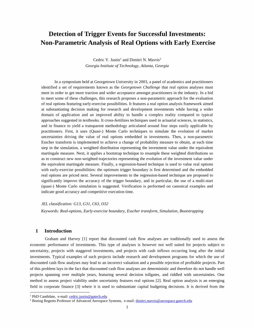
for this purpose. A business model calculator is used next as a “transfer function” representing the value of the

business prospect under review given the state of the uncertainties. This process is illustrated in Figure 1.

Figure 1: Uncertainty modeling and Monte Carlo simulations under the physical probability measure

5

The process is then repeated many times to end up with a distribution (sample) of business prospect values at each

time step in the simulation. The evolution of the business prospect value is simulated under the physical or historical

probability measure since the models used for the evolution of the uncertainties are calibrated using observations

from the market.

2.1.2 Using resampling techniques

There might be cases for which a proper calibration of the stochastic process to the data is challenging. This

is true for complex stochastic behaviors for which high frequency market data must be available such as when jumps

or discontinuities occur. In these cases, resampling techniques which consist in sampling directly from observed data

may be used. Bootstrapping is a popular statistical method whose name was first coined by Efron in his 1979 Rietz

Lecture [10] to describe a resampling technique used to estimate the precision of some statistics such as the mean,

median, or standard deviation of a distribution. In the original application, bootstrap samples were constructed by

sampling with replacement a subset of an original distribution and statistics of interest were then computed. For the

simulation of uncertainties, the essence of the bootstrap method is retained but the application is different: similarly,

the bootstrap method is used to sample with replacement from an original distribution (empirical sample) but what is

new is that the bootstrap sample is used next to generate trajectories representing the evolution of uncertainties. Like

in the Monte Carlo simulation approach, a business model calculator is used next as a “transfer function”

representing the value of the business prospect given the state of the uncertainties at each time step in the simulation.

This yields trajectories representing the evolution of the business prospect value over time as shown in Figure 2.

Figure 2: Resampling with bootstrap method

2.2 Change of probability measure with Esscher transform and its non-parametric approximation

For option valuation purposes, the dynamics of the business prospect value must be specified using the

equivalent martingale measure or equivalent risk-neutral probability measure. This enables the computation of the

present value of the real option through a discounting of the payoffs using the risk-free rate of return. A change of

probability measure is therefore required. The equivalent martingale measure is a probability measure for which the

returns of all assets are exactly the risk-free rate of return. Mathematically, this is equivalent to subtracting the risk-

premium from the expected returns which makes investors indifferent towards risk, hence the name of the measure.

2.2.1 Using Esscher transform

A change of probability measure technique was proposed in 1994 by Gerber and Shiu [11] to handle a wide

variety of processes featuring stationary and independent increments such as Wiener processes, Poisson processes,

Gamma processes, and inverse Gaussian processes. A transformation based on the Esscher transform [12], a time-

6

honored tool in actuarial finance pioneered by Swedish mathematician Fredrik Esscher and publicized by Kahn [13],

is used to induce an equivalent probability measure. For a probability density function f and a real number h, the

Esscher transform 𝑓𝐸𝑠𝑠 with parameter h is expressed using 𝑀 the moment generating function of f shown in Eq. 1:

𝑓𝐸𝑠𝑠(𝑥, ℎ) =𝑒ℎ𝑥𝑓(𝑥)

𝑀(ℎ), 𝑤𝑖𝑡ℎ ℎ ∈ ℝ 𝑎𝑛𝑑 𝑀(ℎ) = ∫ 𝑒ℎ𝑥𝑓(𝑥)𝑑𝑥

∞

−∞

Eq. 1

Looking at this definition, the Esscher transform is the product of an exponential function and a density function,

normalized by a moment generating function. As a result, this transformation induces an equivalent probability

measure as both distributions agree on sets with probability zero. It also becomes clear why the Esscher transform is

sometimes called exponential tilting: the transformation distorts the original probability measure using an

exponential function. The aim of Gerber and Shiu is to use the free parameter h introduced by the Esscher transform

to ensure that the new probability measure is an equivalent martingale measure. In other terms, the parameter h is

determined to ensure that the discounted business prospect value is a martingale which means that the value of the

underlying business prospect is exactly its expected discounted payoff. When markets are complete, the equivalent

martingale measure is unique and therefore the Esscher transform yields the unique arbitrage-free price for the real

option. The marketed asset disclaimer assumption [14] ensures that the market is complete and therefore that a

unique price for the real option can be found. On the other hand, when the market is incomplete, the claim is not

attainable and there is no possibility for the market and its arbitrageurs to enforce a no-arbitrage price.

Mathematically, there may be many equivalent martingale measures and the practitioner has to select one of them.

Several equivalent measures [15] have been proposed such as the minimal martingale measure [16], the minimal

entropy martingale measure [17], the utility martingale measure [17], and of course, the Esscher martingale measure.

Each of them corresponds to a different attitude towards risk and consequently some assumptions regarding the

preferences and risk attitude of decision-makers must be set to pick which utility function and therefore which

equivalent martingale measure is most appropriate. In fact, in the discussion pertaining to their paper [18], Gerber

and Shiu show that the Esscher martingale measure is consistent with investors or decision-makers exhibiting power

utility behaviors3. Power utility functions, also known as iso-elastic utility functions, have the property of constant

relative risk aversion which means that the risk aversion is independent of the level of initial wealth. The power

utility assumption has the advantage of being consistent with some other fundamental results of finance and

economics (mutual fund theorem in Cass and Stiglitz [19] and Stiglitz [20] for instance). Surprisingly, the Esscher

transformation has never been used for real option analysis to the authors’ knowledge.

2.2.2 Using the non-parametric approximation of the Esscher transform

A significant hurdle is that the Esscher transform as introduced above requires an explicit formulation for

the probability density function f representing the distribution of the business prospect value at a given point in time.

While it may be known to the practitioner in some simple cases, most of the times analysts have little or no

information as to the distribution of the business prospect value once all uncertainties are mixed in the business

prospect value computation. In fact, one major objective of this research is to enable option valuation without the

need to specify a parametric model (i.e. time-indexed distributions) for the underlying business prospect value

because of the high subjectivity involved when selecting models that are not directly observable in the market.

3 A power utility function belongs to the class of hyperbolic absolute risk aversion utility functions. It is a special

case in that it exhibits a constant relative risk aversion. The power utility function relates the utility U to the level of

consumption c using the following formula with 𝜂 a constant measuring risk-aversion:

𝑈(𝑐) = {𝑐1−𝜂−1

1−𝜂𝜂 > 0, 𝜂 ≠ 1

ln(𝑐) 𝜂 = 1

7

Adapting the Esscher transformation technique so that it does not require the explicit formulation of the underlying

stochastic process (and its associated distribution at each time step) would prove particularly useful for real option

analysis. Pereira, Epprecht, and Veiga [21] propose a model-free, non-parametric approximation of the Esscher

transform presented previously to transform the behavior of an underlying asset from the physical probability

measure to the equivalent martingale measure. The technique is geared towards the pricing of financial options and

needs to be adapted for the economic evaluation of corporate investments featuring flexibility.

The first step of the non-parametric Esscher transformation starts with the collection of the n business

prospect values 𝑆𝑡𝑗=1..𝑛

at a given time cross-section t. This data may have either one of two origins: it can be

directly observable and available (such as the market price of the underlying asset) or it can be generated by the

practitioner if the underlying asset is synthetic and not publicly traded. These values are used to estimate the n

continuously compounded rates of return 𝑥𝑡𝑗=1..𝑛

of the business prospect value. Let’s now call 𝑋�̂� the vector of size

n containing these n rates of return from the (unknown) business prospect return distribution at time t as shown in

Eq. 2:

𝑋�̂� = [𝑥𝑡1, 𝑥𝑡

2, 𝑥𝑡3… 𝑥𝑡

𝑛] = [𝑙𝑛 (𝑆𝑡1

𝑆𝑡−11 ) , 𝑙𝑛 (

𝑆𝑡2

𝑆𝑡−12 ) , 𝑙𝑛 (

𝑆𝑡3

𝑆𝑡−13 )… 𝑙𝑛 (

𝑆𝑡𝑛

𝑆𝑡−1𝑛 )] Eq. 2

The second step consists in the computation of the empirical moment generating function which is

estimated using Eq. 3:

𝑀�̂�(ℎ, 𝑡) =1

𝑛∑𝑒ℎ𝑥𝑡

𝑖

𝑛

𝑖=1

Eq. 3

The third step is directly inspired by the work of Gerber and Shiu in that it solves for the specific value of

the parameter h such that the asset price is a martingale under the new probability measure. This specific parameter

value, denoted h*, solves Eq. 4 and in a complete market with no arbitrage, the fundamental theorem of asset pricing

[22] ensures that this solution is unique.

𝑒𝑟𝑓 =∑ 𝑒(ℎ

∗+1)𝑥𝑡𝑖𝑛

𝑖=1

∑ 𝑒ℎ∗𝑥𝑡𝑖𝑛

𝑖=1

Eq. 4

With the proper value h* of the Esscher transform parameter, the final step consists in constructing the new

probability measure. This is done by reweighting each observation and ensuring that their probabilities sum to one.

The new probability vector giving the probability of each observation under the new measure is given by Eq. 5. This

is the set of probabilities that is used for the pricing of options and for the computation of expectations.

ℚ𝑡ℎ∗ = [

𝑒ℎ∗𝑥𝑡1

∑ 𝑒ℎ∗𝑥𝑡𝑖𝑛

𝑖=1

,𝑒ℎ

∗𝑥𝑡2

∑ 𝑒ℎ∗𝑥𝑡𝑖𝑛

𝑖=1

… 𝑒ℎ

∗𝑥𝑡𝑛

∑ 𝑒ℎ∗𝑥𝑡𝑖𝑛

𝑖=1

] Eq. 5

In summary, the non-parametric Esscher transform enables practitioners to distort an unknown probability

distribution into a risk-neutral probability distribution. This transformation is done at each time cross-section in the

simulation and consists of weighting each observation in the cross-section sample. This weighted sample of returns

is converted back to business prospect values and subsequently used to estimate the expected option payoff which is

discounted to the present time using the risk-free interest rate. Provided mild conditions of stationarity and

increment independence are satisfied, the non-parametric Esscher transform tremendously simplifies the analyses of

practitioners who no longer need to calibrate and substantiate the choice of one particular stochastic process for the

8

usually unknown evolution of the business prospect value. The algorithm to perform the change of measure is

depicted in Figure 3.

Figure 3: Non-parametric Esscher transform for change of probability measure

2.3 Resampling using the bootstrap technique

The non-parametric Esscher transform enables a change of probability measure and the expression of the

evolution of the business prospect value under the equivalent martingale measure, a necessary step for option pricing

using simulation. The technique changes the mean of the business prospect value distribution at each intermediate

step by reweighting the different outcomes. In other words, the procedure described so far yields different sets of

weights at each intermediate time step in the simulation. Thus, a given trajectory is made of time-indexed

observations that have different weights attached to each observation. As much as the procedure is suitable for

valuing European options for which the weighting may be performed just once at expiration when payoffs are

computed, valuing American or Bermudan options is more difficult since it requires identically weighted

observations at each time cross-section on a trajectory (to perform regressions as will be explained in 2.4).

With this issue in mind, we propose a way forward using a resampling technique while still assuming a

stationary process with independent increments for the evolution of the business prospect value. A single time cross-

section of weighted business prospect returns obtained from the non-parametric Esscher transformation is first

selected. Alternatively, several time cross-sections may be pooled together in order to increase the size of the pooled

sample of returns. The bootstrap technique described previously is then applied to this sample of weighted returns

and consists in repetitive sampling with replacement to generate a new non-weighted sample of returns.

Nevertheless, the weights (or probabilities) associated with each return in the original sample have to be accounted

for when sampling with replacement to ensure that the properties of the equivalent martingale measure are preserved

and carried over to the new trajectories being generated.

This is done by figuratively stacking all the weights in one column, the “height” of which is one since the

weights represent a probability measure. Next, a random number is drawn from a uniform distribution (between zero

and one) to define which level in the column is reached and therefore which piece of the stack is selected. The

selected piece corresponds to a return which is then used to construct a new trajectory as illustrated in Figure 4. In

doing so, returns with larger weights (probabilities) have a greater chance of being drawn while returns with smaller

weights (probabilities) have less chance of being drawn during the resampling effort. Starting with an initial

9

business prospect value, the resampling of returns enables the construction of trajectories representing the evolution

of the business prospect value under the new equivalent martingale measure.

Figure 4: Bootstrapping weighted observations by first stacking weights and then sampling randomly from the stack

(mapping between position in the stack and return value is known)

2.4 American option valuation and construction of the trigger boundary

This step is articulated around two objectives: the first consists in identifying when and under which

circumstances it becomes optimal to invest in a business prospect featuring managerial flexibility, while the other

consists in assessing the value of the real option.

2.4.1 Using least-squares Monte Carlo technique

For real option applications, Monte Carlo simulations enable the capture of a multitude of uncertainties and their

interdependencies. However, pricing real options using Monte Carlo simulations has long been hindered by the

perceived inability of simulation techniques to correctly handle path-dependent options [23]. Indeed, the value of the

American option at the kth time step 𝑡𝑘 denoted 𝑉𝑡𝑘 on an asset S with observed value 𝑆𝑡𝑘 and with payoff function P

can be expressed as the maximum between exercising immediately and holding the option as shown in Eq. 6. In

other words, while marching forward in time, one has to compare the payoff earned from immediate exercise to the

value of holding the option for at least one extra step. However, at time 𝑡𝑘 there is yet no estimate of the present

value of the one-period-ahead option value 𝑉𝑡𝑘+1.

𝑉𝑡𝑘 = 𝑚𝑎𝑥[𝑃(𝑆𝑡𝑘), 𝑒−𝑟𝑓(𝑡𝑘+1−𝑡𝑘)𝐸ℚ(𝑉𝑡𝑘+1|𝑆𝑡𝑘)] Eq. 6

Fortunately, this paradigm has evolved starting in 1993 with the paper of Tilley [24] which aims was to

dispel the belief that American-style options could not be valued using simulations. A significant improvement came

in 1996 with the work of Carriere [25] regarding the valuation of options with early-exercise properties. Faced with

the same problem of estimating the one-period-ahead option value for subsequent comparison with the immediate

exercise payoff, Carriere suggests the use of non-parametric regressions to regress the conditional expectation and

therefore to estimate the value of holding the options. As noted by Stentoft [26], the reason for this regression is that

a conditional expectation is a function and “any function belonging to a separable Hilbert space may be represented

as a countable linear combination of basis-functions for the space.” Consequently, let’s introduce {𝜙𝑖}1∞ as a family

of basis-functions for that space. The expectation may be rewritten and approximated using the first M basis-

functions {𝜙𝑖}𝑖=1𝑀 as shown in Eq. 7:

Step 2:

Representation of

distribution on [0,1] scale

Step 1:

Weighted

observations(Initial population)

Step 3:

Sampling from

population with replacement

WeightsTrajectories0

1

Representation

Sample

Step 4:

Construction of

trajectories using values from sampling

Trajectory from sample

10

𝐸ℚ(𝑉𝑡𝑘+1|𝑆𝑡𝑘) = ∑𝛼𝑖(𝑡𝑘) ∙ 𝜙𝑖(𝑆𝑡𝑘)

∞

𝑖=1

~∑𝛼𝑖(𝑡𝑘) ∙ 𝜙𝑖(𝑆𝑡𝑘)

𝑀

𝑖=1

Eq. 7

Any family of basis-functions should work but Carriere suggests using either splines or a polynomial

smoother. Next task is the estimation of the coefficients 𝛼𝑖 of the linear combination. This is done marching

backward, starting at expiration and moving back until the present time: at expiration, the value of the option is

exactly the payoff, while for all preceding time steps denoted 𝑡𝑘 a regression is performed using the observations of

the underlying value for the n simulated trajectories denoted 𝑆𝑡𝑘𝑗=1..𝑛

as well as the continuation value 𝑉𝑡𝑘+1𝑗=1..𝑛

(a

conditional expectation). The regression objective is to select a family of coefficients {𝛼𝑖}1𝑀 that minimizes the error

between the regressed conditional expectations and the option values across the n simulated trajectories. This error is

defined in Eq. 8:

min{𝛼𝑖}0

𝑀∑(∑𝛼𝑖(𝑡𝑘) ∙ 𝜙𝑖(𝑆𝑡𝑘

𝑗) − 𝑉𝑡𝑘+1

𝑗

𝑀

𝑖=1

)

𝑛

𝑗=1

2

Eq. 8

The immediate exercise value at time 𝑡𝑘 denoted 𝑃(𝑆𝑡𝑘) is compared next to the discounted regressed

conditional expectation to find the option value defined in Eq. 9. The procedure is repeated for each trajectory at

each time step marching back until the present time to find the value of the American option.

𝑉𝑡𝑘 = 𝑚𝑎𝑥 [𝑃(𝑆𝑡𝑘), 𝑒−𝑟𝑓(𝑡𝑘+1−𝑡𝑘)∑𝛼𝑖(𝑡𝑘) ∙ 𝜙𝑖(𝑆𝑡𝑘)

𝑀

𝑖=1

] Eq. 9

The algorithm for American option valuation using simulation and regression techniques is depicted in

Figure 5. A popular enhancement to this work is the least-squares Monte Carlo approach of Longstaff and Schwartz

[27]. Dating back to 2001, this approach is very similar to the method of Carriere except for two facts: the algorithm

uses a least-squares regression and the regression is made using only in-the-money paths. In the Longstaff-Schwartz

method, the proposed regression uses an ordinary least-squares technique to regress the conditional expectation

𝐸ℚ(𝑉𝑡𝑘+1|𝑆𝑡𝑘) against a set of explanatory variables. The set of explanatory variables is a family of basis-functions

denoted {𝜙𝑖}1𝑀 and valued using the conditioning underlying asset price 𝑆𝑡𝑘. One may use a simple monomial family

{𝜙𝑖: 𝑋 → 𝑋𝑖−1}𝑖=1𝑀 as the family of basis-functions, or some families of orthogonal polynomials such as the

Chebyshev polynomials, the Legendre polynomials, and the Laguerre polynomials. Furthermore, the regression is

performed using only paths that are in-the-money since the decision to exercise or not the option is only relevant

whenever the option is in-the-money. According to Longstaff and Schwartz, “by focusing on the in-the-money

paths, [… this…] limits the region over which the conditional expectation must be estimated, and far fewer basis

functions are needed to obtain an accurate approximation to the conditional expectation function.”

11

Figure 5: American and Bermudan option valuation with regression and trigger boundary generation

A subtle difference with the works of Carriere is the choice of realized payoffs as dependent variables for

the regression instead of using previously computed conditional expectations. These realized payoffs may be

resulting from an early-exercise at the next time step 𝑡𝑘+1 or from an early-exercise several steps down-the

trajectory, for instance at 𝑡𝑘+𝑗 (𝑗 > 1). According to Longstaff and Schwartz, this precludes “an upward bias in the

value of the option”. This means that the conditional expectation at time 𝑡𝑘 denoted by 𝐸ℚ(𝑉𝑡𝑘+1|𝑆𝑡𝑘) is used just

once in the algorithm to check whether the value of holding the option is greater than the value of immediate

exercise. This yields the following exercise rule and option value highlighted in Eq. 10. Let’s notice the subtle

difference with Eq. 9 in the value of the option (the exercise rule remains the same).

𝑉𝑡𝑘 =

{

𝑃(𝑆𝑡𝑘) , 𝑖𝑓 𝑃(𝑆𝑡𝑘) ≥ 𝑒

−𝑟𝑓(𝑡𝑘+1−𝑡𝑘)∑𝛼𝑖(𝑡𝑘) ∙ 𝜙𝑖(𝑆𝑡𝑘)

𝑀

𝑖=1

𝑒−𝑟𝑓(𝑡𝑘+1−𝑡𝑘) ∙ 𝑉𝑡𝑘+1 , 𝑖𝑓 𝑃(𝑆𝑡𝑘) < 𝑒−𝑟𝑓(𝑡𝑘+1−𝑡𝑘)∑𝛼𝑖(𝑡𝑘) ∙ 𝜙𝑖(𝑆𝑡𝑘)

𝑀

𝑖=1

Eq. 10

2.4.2 Generating the trigger boundary

The next objective is to solve for the trigger boundary in order to provide decision-makers with relevant

data to substantiate whether investing now or later is optimal. The trigger boundary is made of critical prices which

are defined as the time-indexed business prospect values such that keeping the real option open (waiting) has the

same value as exercising the option immediately (investing). Using the conditional expectation regressions obtained

in the Longstaff-Schwartz algorithm, the critical prices 𝑆𝑡𝑘𝐶 are obtained at each time step 𝑡𝑘 by solving Eq. 11.

𝑃(𝑆𝑡𝑘𝐶 ) = 𝑒−𝑟𝑓(𝑡𝑘+1−𝑡𝑘)∑𝛼𝑖(𝑡𝑘) ∙ 𝜙𝑖(𝑆𝑡𝑘

𝐶 )

𝑀

𝑖=1

Eq. 11

2.4.1 Estimating the expected time to trigger and the probability of trigger

Once the early exercise boundary location is known, the expected time to hit the trigger boundary

conditional on hitting it, as well as the actual probability of exercising the real option can be computed using (Quasi-

) Monte Carlo simulations as highlighted in Eq. 12. In this equation, 𝐸(𝜏) is the expected time to hit the trigger

boundary, 𝑃𝐸𝑥𝑒𝑟𝑐𝑖𝑠𝑒 is the probability of hitting the trigger boundary, 𝜏 is the discrete-time equivalent of a stopping

12

time, T is the maturity of the option, n is the number of trajectories in the simulation, while 𝑛∗ is the number of

trajectories hitting the trigger boundary. The simulations are carried out under the physical probability measure since

the expected time to hit and the probability of hitting depend on the real drift of the stochastic process. The expected

time to hit the boundary is interesting as it gives an indication of how much time is available before the company is

expected to invest: in the case of R&D programs, the expected time to hit the trigger boundary suggests the time left

to improve the performance and mature technologies that are projected to be used during the development.

𝐸(𝜏) =1

𝑛∗∑𝜏𝑖 ∙ 𝟏 𝜏𝑖≤𝑇

𝑛

𝑖=1

𝑎𝑛𝑑 𝑃𝐸𝑥𝑒𝑟𝑐𝑖𝑠𝑒 =𝑛∗

𝑛

𝑤𝑖𝑡ℎ: 𝜏𝑖 = min𝑘(𝑡𝑘 ≥ 0 / 𝑆𝑡𝑘

𝑖 ≥ 𝑆𝑡𝑘𝐶 ) 𝑎𝑛𝑑 𝑛∗ =∑𝟏 𝜏𝑖≤𝑇

𝑛

𝑖=1

Eq. 12

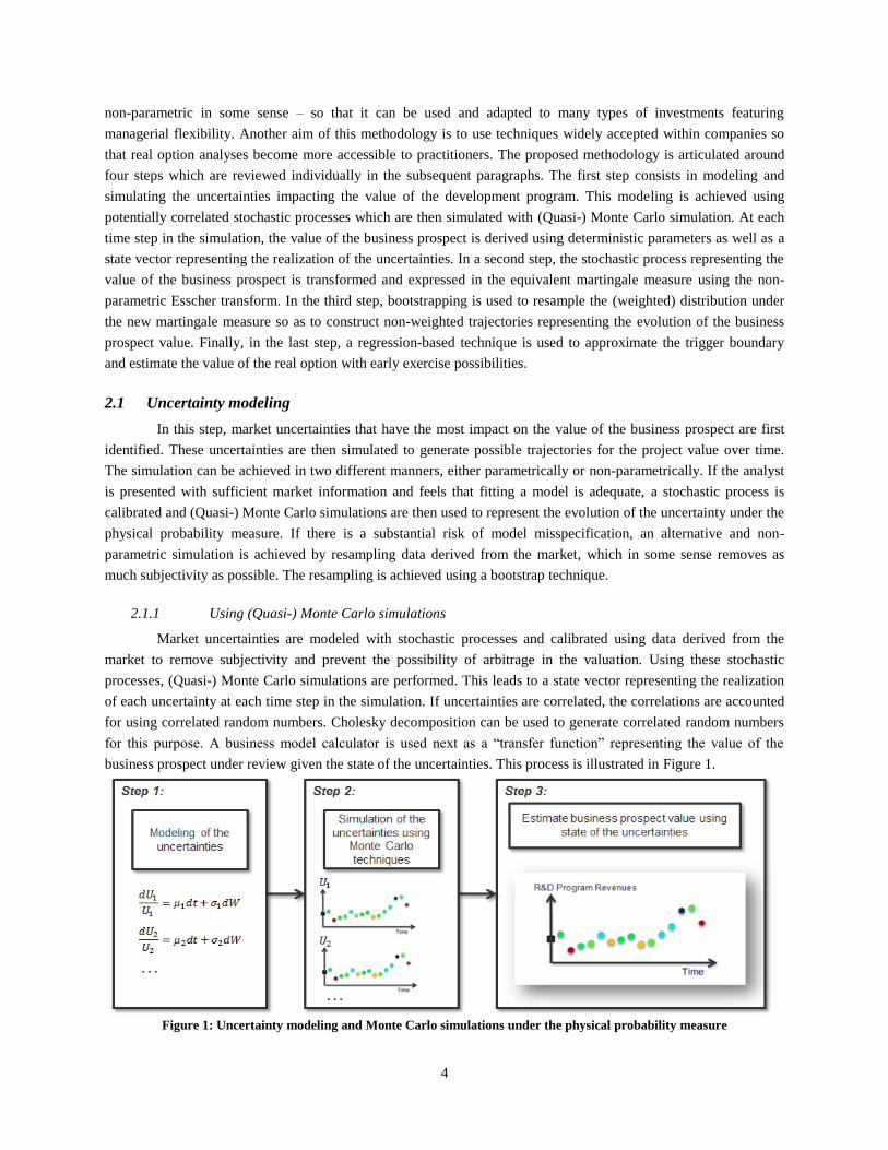
2.5 Summary of the proposed methodology

Having described the different steps of the proposed methodology to value real options with early-exercise

privileges, the diagram in Figure 6 summarizes the techniques used and depicts the flow of information between the

various steps.

Figure 6: Main steps of the proposed methodology

13

2.6 Meeting the Georgetown Challenge?

This article started with the Georgetown Challenge (Copeland and Antikarov [9]) which is a set of

requirements identified by academics and practitioners that real option analyses must meet in order to get wider

acceptance. In the previous section, a methodology is constructed step-by-step to analyze long-term staggered

corporate investments featuring flexibility. It is therefore appropriate to revisit these key challenges identified earlier

and to verify whether the proposed way-forward meets some of these requirements. Table 2 maps the requirements

of the Georgetown Challenge as well as some specific challenges identified as part of this research, to the

assumptions, techniques, and solutions shaping the proposed methodology.

14

Table 2: Addressing the challenges facing the analysis of long-term corporate investment programs featuring flexibility

Monte Carlo-based and non-parametric Esscher-transformed real option approach

Geo

rget

ow

n C

hall

enge

Req

uir

emen

ts

(Adap

ted f

rom

Copel

and a

nd A

nti

kar

ov [

9])

Intuitively dominate other decision-

making methods

Ability to capture the flexibility in decision-making

Recognize the value created by active and astute management

Capture the reality of the problem Ability to handle optimum timing issues related to decision-making using American-type options

Ability to handle staggered investment programs with decision gates using compound options

Use mathematics that everyone can

understand

Esscher transform ensures that risk-neutralization is performed in a transparent and tractable way

Non-parametric Esscher transform removes the requirement to calibrate complex models

Rule out the possibility of mispricing

by eliminating arbitrage

Esscher transform provides the price that would be enforced by arbitrageurs in a complete market

Esscher transform provides the price corresponding to the preference of economic agents with iso-

elastic utility functions in the case of incomplete markets

Be empirically testable Tough requirements as there are no published transacted price for these investments

Only heuristic argumentation can substantiate whether the method provides acceptable solutions

Appropriately incorporate risk Handling of technical and market risks separately, with technical risk analyzed with decision trees

Possibly difficult to estimate volatilities of some particular risks if no prior history exists

Use as much market information as

possible

Ability to use market information whenever possible to model the dynamics of the uncertainties

driving the development program value

Ad

dit

ion

al r

equir

emen

ts Ability to capture a complex reality

with intertwined uncertainties

Monte Carlo simulations allow the use of many different stochastic behaviors for uncertainties

Monte Carlo simulations allow the modeling of correlations between some sources of uncertainties

Ability to visualize uncertainties and

the decision process

Visualization of the evolution of uncertainties affecting the decision process

Visualization of the evolution of the development program value over time

Ability to handle corporate

investments featuring exotic options

Recent Monte Carlo methods allow analyses of programs with potentially moving decision tollgates

and therefore the search for optimum investment timeframes

Ability to converge to a solution in a

timely manner

Use of bootstrapping methods allow a reduction in computation time to generate trajectories of

program values used for Monte Carlo simulations

15

3 Lessons Learnt and Implementation

Preliminary experimentations indicate that the proposed methodology works very well, especially for the

valuation of real options. However, the generation of the trigger boundaries using simulation and regressions yields

noisy results. Indeed, the nature of Monte Carlo simulations as well as numerical errors introduced by conditional

expectation regressions lead to trigger boundaries with jaggies and undesirable local non-monotonicity. This is to be

expected and the inaccuracies of trigger boundaries obtained in this manner have been documented in the literature

which usually suggests the use of finite-difference methods to obtain reliable and accurate boundaries. However,

because the proposed real option framework enables the study of a wide variety of potentially correlated and multi-

dimensional stochastic processes, simulation remains an appealing option. As a result, further research is carried out

to improve the ability of the least-squares Monte Carlo algorithm to provide better trigger boundaries.

3.1 Refinements to the Longstaff-Schwartz least-squares Monte Carlo algorithm

3.1.1 Control variates sampled at exercise of the real option

The first refinement to the regression-based algorithm consists in using control variates sampled at exercise

of the real option. Control variates enable a reduction in the variance of estimates obtained through Monte Carlo

simulations by exploiting errors in estimates of known quantities. For instance, it is usual to have the price of a

European option as control variate during the pricing of an American option. In this case, the European option price

is computed using the same set of trajectories as those used for the pricing of the American option and the European

option price estimate 𝑉𝑡0𝐸𝑀𝐶 is compared to its known closed-form solution 𝑉𝑡0

𝐸 to compute its error. This error is used

next to correct the estimate of the American option price 𝑉𝑡0𝐴_𝑀𝐶

as shown in Eq. 13.

𝑉𝑡0𝐴 = 𝑉𝑡0

𝐴_𝑀𝐶 + 𝜃 ∙ (𝑉𝑡0𝐸𝑀𝐶 − 𝑉𝑡0

𝐸) , 𝑤𝑖𝑡ℎ 𝜃 =−𝐶𝑜𝑣(𝑉𝑡0

𝐴_𝑀𝐶 , 𝑉𝑡0𝐸𝑀𝐶)

𝑉𝑎𝑟 (𝑉𝑡0𝐸𝑀𝐶)

Eq. 13

However, control variates sampled at maturity are not efficient for the pricing of options featuring early-

exercise possibilities because the correlation between the control variates (sampled at maturity) and the payoffs

(sampled at the stopping time) is not large. To improve this correlation, Rasmussen [28] suggests a different

sampling scheme for the control variates: instead of sampling the control variates at maturity, the control variates are

sampled for each and every simulation path individually at the time of exercise of the American option. This process

is highlighted in Figure 7.

Figure 7: Sampling control variates at maturity (left graph) is less correlated with option payoffs than sampling

control variates at exercise (right graph)

0

1

2

3

0 12 24 36 48 60

Triggerboundary

Control variate sampling

0

1

2

3

0 12 24 36 48 60

Triggerboundary

Control variate sampling

16

Since the aim of the proposed real option methodology is to stay as generic as possible and because the

stochastic process representing the evolution of the business prospect value is unknown, using the European option

price as control variate is not possible as this quantity is unknown. Instead, we suggest using the discounted business

prospect value, which is a martingale by construction, as control variate. The optional stopping theorem ensures that

the expected value of the discounted business prospect value at a stopping time is its (known) initial value.

Furthermore, Rasmussen argues [29] that the continuation value regressions may be improved in order to

enhance the generation of the trigger boundary. Indeed, if there is a time 𝑡𝑘 variable for which the time 𝑡𝑘−1

conditional expectation is known, then the time 𝑡𝑘 variable can be projected onto the same set of basis-functions as

those used for the projection of the discounted continuation value and then compared to the 𝑡𝑘−1 conditional

expectation. The error between the projection and the conditional expectation is then used to improve the regression

of the discounted continuation value. Again, we suggest using the discounted business prospect value since it is a

martingale and therefore its 𝑡𝑘−1 conditional expectation is always known.

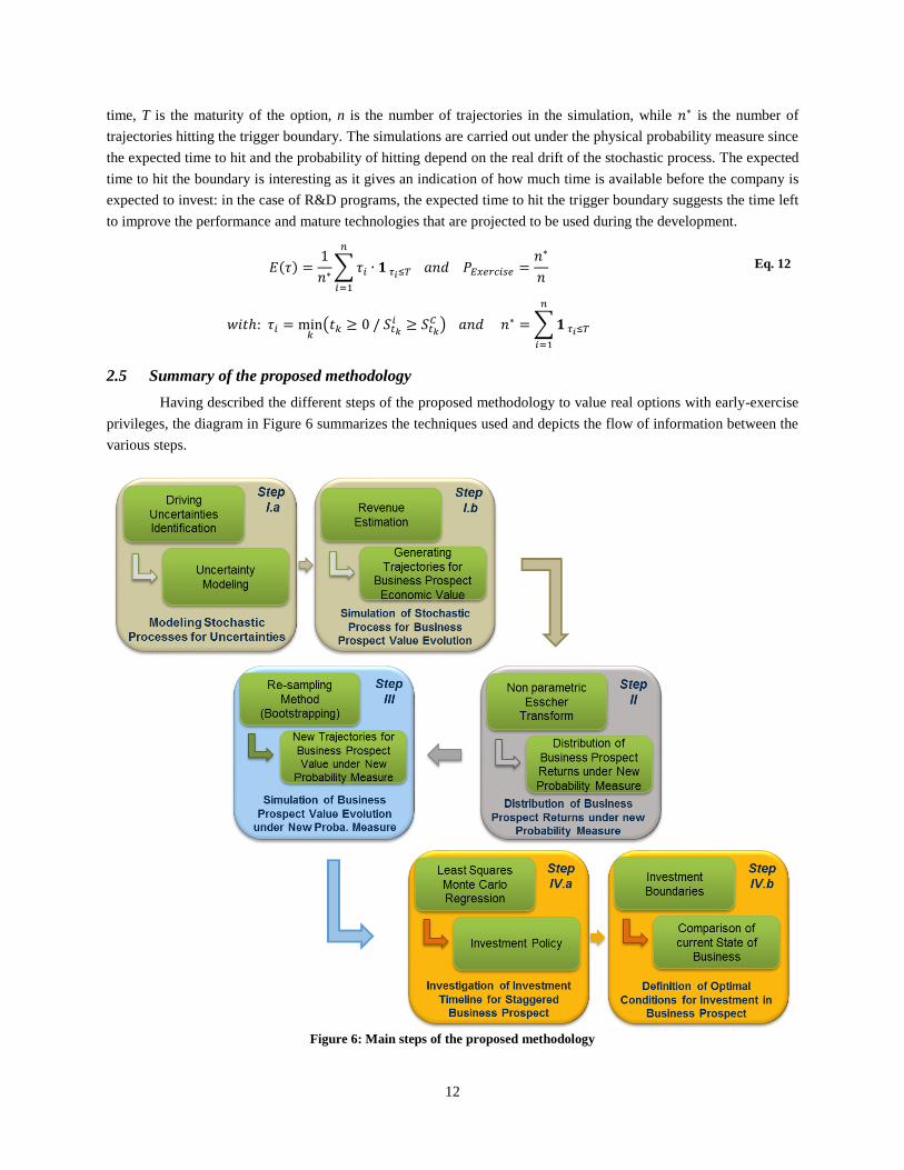
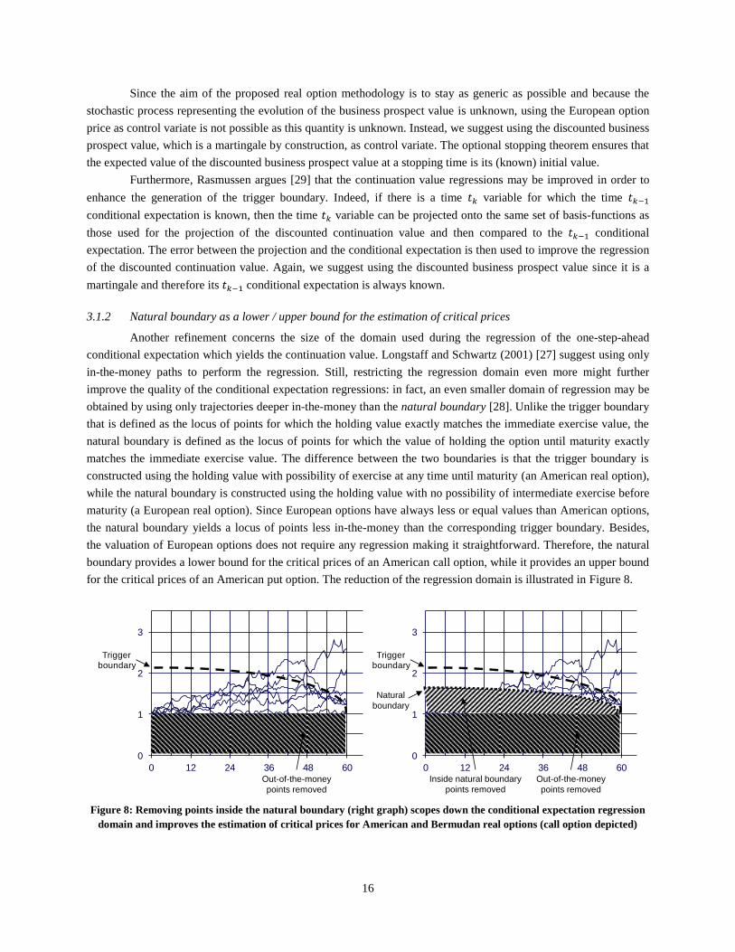
3.1.2 Natural boundary as a lower / upper bound for the estimation of critical prices

Another refinement concerns the size of the domain used during the regression of the one-step-ahead

conditional expectation which yields the continuation value. Longstaff and Schwartz (2001) [27] suggest using only

in-the-money paths to perform the regression. Still, restricting the regression domain even more might further

improve the quality of the conditional expectation regressions: in fact, an even smaller domain of regression may be

obtained by using only trajectories deeper in-the-money than the natural boundary [28]. Unlike the trigger boundary

that is defined as the locus of points for which the holding value exactly matches the immediate exercise value, the

natural boundary is defined as the locus of points for which the value of holding the option until maturity exactly

matches the immediate exercise value. The difference between the two boundaries is that the trigger boundary is

constructed using the holding value with possibility of exercise at any time until maturity (an American real option),

while the natural boundary is constructed using the holding value with no possibility of intermediate exercise before

maturity (a European real option). Since European options have always less or equal values than American options,

the natural boundary yields a locus of points less in-the-money than the corresponding trigger boundary. Besides,

the valuation of European options does not require any regression making it straightforward. Therefore, the natural

boundary provides a lower bound for the critical prices of an American call option, while it provides an upper bound

for the critical prices of an American put option. The reduction of the regression domain is illustrated in Figure 8.

Figure 8: Removing points inside the natural boundary (right graph) scopes down the conditional expectation regression

domain and improves the estimation of critical prices for American and Bermudan real options (call option depicted)

0

1

2

3

0 12 24 36 48 60

Triggerboundary

Natural

boundary

Out-of-the-money

points removed

Inside natural boundary

points removed

0

1

2

3

0 12 24 36 48 60

Triggerboundary

Out-of-the-money

points removed

17

The natural boundary can be efficiently computed via simulation, starting right before maturity and

marching back in time using just one set of trajectories (in fact a single set of returns from a complete simulation).

At each time step 𝑡𝑘 starting from the next to last one, bisection is used to search for the value of the business

prospect 𝑆𝑡𝑘 such that the European option price 𝑉𝑡𝑘𝐸𝑀𝐶 is equal to the option immediate payoff 𝑃 as shown in Eq. 14.

At each time step, multiple European option prices must therefore be computed during the search procedure (same

option but different spot prices). For each 𝑡𝑘 option, the computation is carried out with the same set of returns but

with a different simulation starting point. For instance, right before expiration, the European options have a one-step

maturity and therefore only returns associated with the first time step of the trajectories are used. For the preceding

step, the European options have a two-step maturity and therefore only returns associated with the first two time

steps of the trajectories are used. Depending on the accuracy sought for the natural boundary, the procedure is

repeated either at every time step or every couple of time steps while marching back in time.

𝑉𝑡𝑘𝐸𝑀𝐶(𝑆𝑡𝑘) = 𝑃(𝑆𝑡𝑘) Eq. 14

3.1.3 Multi-start Monte Carlo simulations

The generation of the trigger boundary using Monte Carlo simulations is a notoriously difficult task. The

proposed multi-start Monte Carlo improvement stems from the observation that the quality of the least-squares

regressions improves as more points and therefore more trajectories lie “in-the-money”. Indeed, with more

trajectories “in-the-money”, the regression of the conditional expectation becomes more accurate as more

trajectories are likely to cross the trigger boundary thus enhancing the estimation of the critical price. In fact, even

when the trigger boundary is reasonably well approximated as a whole, the approximation deteriorates close to the

starting time of the simulation. This is a problem of interpolation and extrapolation when searching for the critical

price using the conditional expectation regressions. Close to the beginning of the simulation, the effects of diffusion

are limited and the business prospect values generated and used for the regression of the conditional expectation are

not dispersed enough to encompass or at least to be close to the critical price. Rasmussen [30] suggests starting the

simulation prior to the current time (i.e. back in time) in order to let the diffusion artificially disperse the data points

and therefore “to provide sufficient in-the-money observations to estimate the exercise boundary”.

Even though this is a step in the right direction, this solution does not go far enough and we suggest several

improvements. First, the objective should not be to provide a sufficient number of in-the-money observations but

rather to provide a sufficient number of observations close to the unknown early-exercise boundary so as to avoid

extrapolations during the critical price search since extrapolations are notoriously bad for polynomial regressions

(Runge’s phenomenon). Next, this approach is not very efficient computationally-wise as a longer clock-time must

be simulated to accommodate the back-in-time starting point. In the generic environment proposed in this paper, this

is computationally costly due to the need for resampling. Finally, this approach does not guarantee that the

dispersion is sufficient to provide observations close to the critical price. In fact, for at-the-money call options with

low risk-free rates and large volatilities, the drift of a geometric Brownian motion under the equivalent martingale

measure is usually negative and the proposed approach tends to drive trajectories away from the initial critical prices

of the trigger boundary.

Instead, we suggest a multi-start Monte Carlo simulation. The is based on the fact that the position of the

trigger boundary is not affected by the initial business prospect value and that using different starting points for the

simulations should yield the same boundary. In the multi-start Monte Carlo, we suggest using m different starting

points, each having 𝑛/𝑚 simulations attached, instead of having n simulations starting from a single point in the

past. As such, the technique illustrated in Figure 9 does not increase the computational burden. The starting points

are chosen so as to maximize the likelihood of “encompassing” the early-exercise boundary while minimizing the

18

likelihood of sampling the domain where early-exercise is not optimal. This leads to the question of selecting

appropriate starting points: the strike price and a multiple of the strike can almost always be used to select two

extreme starting points. The initial point of the natural boundary derived previously provides another excellent

lowest (largest) starting point for call (put) options. Finally, the domain in between these extreme starting points is

evenly distributed to get evenly-spaced simulation starting points.

Figure 9: Multi-start simulations enable more interpolations and fewer extrapolations during the critical price search

using the one-step-ahead conditional expectation regressions

3.1.4 Quasi-Monte Carlo simulations using low-discrepancy Sobol sequence

Despite the implementation of the previous refinements, there is still some variability in the shape and

position of the trigger boundary when repeating identical Monte Carlo experiments. The variability is induced by

changes in the seeds used by pseudo-random number generators. The modifications of the trigger boundary shape

and position observed during repeated experiments can be attributed to the varying quality of the sequences of

pseudo-random numbers used. Consequently, one refinement of the methodology concerns the use of low-

discrepancy sequences instead of pseudo-random numbers to generate trajectories of the primary uncertainties under

the physical probability measure. Indeed, Jackel [31] argues that low-discrepancy sequences provide superior

performance when trying to generate uniformly distributed numbers for the purpose of inverse transform sampling.

Figure 10: 20,000 uniformly distributed sequences of numbers across two dimensions. Left graph represents

pseudo-random numbers from a Mersenne Twister while right graph represents Sobol sequence

0

1

2

3

0 12 24 36 48 60

Starting Points

InterpolationInterpolationExtrapolation

0

1

2

3

0 12 24 36 48 60

Triggerboundary

0

0.2

0.4

0.6

0.8

1

0 0.2 0.4 0.6 0.8 1

0

0.2

0.4

0.6

0.8

1

0 0.2 0.4 0.6 0.8 1

19

This is illustrated in Figure 10 which compares a two-dimensional set of uniformly distributed numbers

using the Mersenne Twister implemented within the MS Excel environment and a two-dimensional Sobol sequence:

pseudo-random numbers exhibit gaps and clustering while Sobol sequences are evenly distributed. Several low

discrepancy sequences may be used for the purpose of Quasi-Monte Carlo simulations like the Van-der-Corput

sequence, the Halton sequence, the Niederreiter sequences, and the Sobol sequences [32]. However, many of these

sequences are not well suited for high-dimensional applications such as path-dependent options: indeed, each time

step represents one dimension and therefore path-dependent options may have several hundred dimensions.

Nevertheless, Sobol et al. [33] argue that properly initialized Sobol sequences may be used in high dimension

applications. As a result, these sequences are used for this research. Finally, Jackel [31] indicates that the

convergence of Quasi-Monte Carlo simulations is not one over the square root of the number of samples (as in

traditional Monte Carlo simulations) but rather closer to one over the number of samples which leads to a substantial

gain in computational efficiency.

3.1.5 Other refinements

Several other refinements are implemented in order to improve the accuracy of the proposed methodology.

Because they have less impact on the generation of the early-exercise boundary and the estimation of the final

option price, these improvements are only briefly mentioned:

Pooling of Esscher-transformed return samples

In order to increase the size of the sample of weighted returns from which the bootstrap procedure performs

the resampling and in order to decrease the likelihood of drawing repetitively the same highly weighted

returns, the return samples from several time cross-sections are pooled together. This enables to bootstrap

with a “down-sampling factor” i.e. resampling n observations from a sample of size 𝑘 ∙ 𝑛 with 𝑘 an integer

strictly greater than one. This helps mitigate the repetitive sampling of observations with relatively large

weights. In addition, in case rare events such as jumps are present, the pooling of several time cross-

sections increases the likelihood of capturing these rare events, at least in the original sample.

Multi-pass analysis

Several successive analyses are performed in order to remove the upward bias in the Longstaff and

Schwartz algorithm [27]. First, a single set of Quasi-Monte Carlo simulations is used to estimate the natural

boundary. This set of returns is recycled for the multi-start simulations enabling the generation of the

trigger boundary. Finally, a new set of Quasi-Monte Carlo simulations is used to actually value the real

option once the position of the trigger boundary is known.

Restricted early-exercise of the option

Following Rasmussen [29], the early-exercise of the option is performed if and only if the value from

immediate exercise is greater than both the value from holding the option one extra time step and the value

from holding until maturity (i.e. business prospect value is above natural boundary). This is a safeguard to

avoid spurious early-exercise induced by questionable holding value conditional expectation regressions.

Regression of the locus of critical prices

Because the critical prices obtained with the proposed method are noisy and because the trigger boundary is

a smooth monotonous curve when dividends (value leakages in the case of real options) are not discrete,

the critical prices are regressed in order to yield a smooth and monotonous trigger boundary. At maturity

(where a discontinuity may exist), the trigger boundary is fixed to the strike price (investment cost).

20

Multi-pass regression to remove critical-price outliers

The quality of the critical price regression is affected by the presence of outliers. To mitigate the impact of

outliers on the quality of the trigger boundary, the regression is used to compute semi-Studentized residuals

(Studentized residual are computationally intensive to estimate as they require the hat matrix). This enables

the detection of outliers and their removal prior to performing a second improved regression of the critical

prices.

3.2 Implementation choices

In Table 3, the parameters retained for the application and verification of the proposed methodology using

canonical examples are summarized. The methodology is implemented in Visual Basic for Application within the

MS Excel environment to demonstrate the suitability of the method for use by a wide spectrum of practitioners using

development environments typically available to them4.

Table 3: Implementation parameters

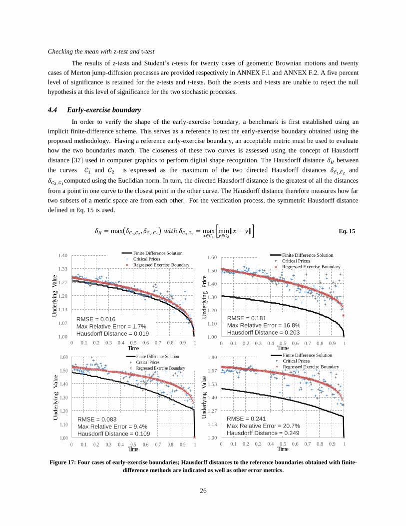
4 Verification and Validation

The purpose of the verification is to check whether the implementation of the real option evaluation

methodology yields correct option prices and accurate trigger boundaries. The similarity between real options and

financial options enables the use of financial options to perform the canonical tests required for the verification of

the proposed method. Indeed, the real option pricing methodology evaluates both types indifferently but the

necessity of “a context” to price real options, the availability of mathematical models to price financial options, and

finally, the prolific literature dealing with the pricing of financial options makes the verification of the later more

straightforward.

4.1 Verification process

The implementation of the proposed real option analysis is articulated around four successive steps

including the Monte Carlo simulation under the physical probability measure, the change of probability measure by

4 Ubiquity of MS Excel and VBA within companies is the prime driver for this choice. Execution time is about sixty

seconds for the combined pricing of a European option, an American option, the generation of the natural boundary,

and the generation of the trigger boundary on a laptop computer featuring an Intel Core i5-3317U processor at

1.7GHz.

Number of paths 80,000 / 50,000 Esscher parameter search

algorithm Bisection

Number of time steps 90 / 180 Esscher parameter

convergence criteria Change less than 1.0E-11

Resampling pool size 4 Least-squares regression

basis 1 ; 𝑃𝑎𝑦𝑜𝑓𝑓 ; 𝑒−𝑃𝑎𝑦𝑜𝑓𝑓

Multi-start simulation

starting point number 50

Critical price search

algorithm

Newton-Raphson

Bisection if N.R. fails

Low discrepancy

sequence Sobol sequence

Trigger boundary

regression basis 1 ; 𝑒−𝜏

0.33 ; √𝜏

time to maturity

Sequence initialization Discard first 4096 points

Randomize

Trigger boundary outlier

removal criteria Semi-Std. Residual >1.96

21

means of Esscher transform, the trajectory resampling using bootstrapping under the new measure, and the least-

squares Monte Carlo technique to generate the trigger boundary and value the option. It is easier to start the

verification process by checking first that the implementation of each individual step performs adequately in a

variety of scenarios before moving on to the verification of the entire implementation. In this regards, the

verification process follows the “bottom-up” approach of the definition-decomposition and verification-validation

V-model diagram. The V-model diagram of Forsberg and Mooz [34] is a graphical representation used in systems

engineering which depicts the activities related to the development lifecycle of complex systems. Several variants of

the V-diagram have been developed over the years [35] including the one highlighted in Figure 11 which describes

adequately a system development process. The model starts with user needs on the upper left and ends with a user

validated system on the upper right. In between, the development process is articulated first in a top-down approach

starting with a requirement analysis with increasing granularity as development progresses, followed by the design,

and leading to the implementation. Next, the development process follows a bottom-up approach as higher levels of

assemblies and subsystems are successively verified, leading to a system-level verification, and finally ending with

the actual operation of the system.

Figure 11: V-Model for systems engineering

Consequently, the different steps of the methodology are verified independently and a verification

capability is thus developed to check their outputs. The verification capability requires different verification

techniques: some steps yield a single number (such as the option price or the Esscher parameter value), while some

steps yield distribution approximations (such as the distribution under the equivalent martingale measure), and

finally some other yield two dimensional curved lines (such as the trigger boundary). The wide spectrum of tests to

be performed can be decomposed into four different types: visual and graphical methods to check the shape of

distributions, statistical tests to check the properties of distributions, similarity tests to check the shape of curves,

and numerical comparisons to check quantitative outputs against published results or well established techniques.

The verification process is described in Figure 12 with dashed arrows representing verifications of individual

modules (subsystem-level) and solid arrows representing verifications of the complete implementation (system-

level).

22

Figure 12: Verification process

4.2 Simulation and non-parametric Esscher transformation

The purpose of the non-parametric Esscher transformation is to transform an arbitrary distribution such that

it exhibits risk-neutral properties. The verification starts with a Monte Carlo simulation of the evolutions of primary

uncertainties affecting the value of the underlying asset which is then simulated under the equivalent martingale

measure using the non-parametric Esscher transform. This yields, at each time step of the simulation, distributions of

both underlying asset values and underlying asset returns. The distribution of returns is compared to the known

theoretical counterpart. Since one requirement for the proposed real option methodology is the ability to capture a

complex reality featuring uncertainties following non-standard stochastic processes, the verification is performed for

two completely different processes: a classic geometric Brownian motion (GBM) for which a single equivalent

martingale measure exists and the Merton jump-diffusion process (JD) for which the equivalent martingale measure

is not unique since the market in incomplete. However, the measure induced by the Esscher transformation leads to

one specific combination of jump-diffusion parameters (i.e. new drift, jump arrival rates, and jump amplitudes)

which are discussed in Schoutens [36].

Q-Q Plots

One popular technique to compare distributions uses quantile-quantile plot also known as Q-Q plot. A Q-Q

plot compares two probability distributions by plotting their quantiles against each other. This non-parametric test

enables a quick visualization of whether the location, scale, and skewness of two probability distributions match. In

this research, the verification is carried out by plotting the quantiles of the terminal distribution induced by the

Monte Carlo simulation and subsequent non-parametric Esscher transformation against the quantiles of the known

theoretical terminal distribution. The results for twenty cases of geometric Brownian motions and twenty cases of

Merton jump-diffusion processes are provided in ANNEX A.1 and ANNEX A.2 respectively.

For the geometric Brownian motions, all of the plots exhibit locus of quantiles almost perfectly on the

bisecting lines. For the Merton jump-diffusion processes, most of the plots are also almost exactly on the bisecting

lines. However some of them exhibit some minor deviations, particularly in the extreme ends of the tails (Cases 2, 3,

6, and 18). This may be related to the difficulty of simulating rare events (jumps) in a finite time simulation. If a Q-

23

Q plot is helpful to qualitatively compare two distributions, it does not however quantify whether the observed

deviations are statistically significant.

Kolmogorov-Smirnov tests

It is indeed interesting to quantify these departures from the bisecting lines so as to perform statistical

testing and potentially reject the equality of terminal distributions hypothesis. Two popular non-parametric tests are

the one-sample and two-sample Kolmogorov-Smirnov tests for the equality between respectively a one-dimensional

distribution and a reference distribution or between two one-dimensional probability distributions. The Kolmogorov-

Smirnov test computes a “distance” between two distribution functions and establishes the corresponding test

statistic. The null hypothesis for these tests is that the samples induced by the simulations followed by non-

parametric Esscher transformations are drawn from the known theoretical distributions. This yields test statistics

(and p-values) that can be compared to critical values to assess the likelihood of observing such difference between

the empirical sample and the reference given the hypothesis that they are sampled from the same distribution.

The results of the Kolmogorov-Smirnov tests for various cases of geometric Brownian motions and Merton

jump-diffusion processes are provided respectively in ANNEX B.1 and ANNEX B.2. One-sample Kolmogorov-

Smirnov tests are used for geometric Brownian motion cases because the terminal distributions are known, while

two-sample Kolmogorov-Smirnov tests are used for Merton jump-diffusion processes since a close-form analytical

expression for the terminal distribution is not available and simulation is used to generate reference samples. A five

percent level of significance is retained for these tests and the Kolmogorov-Smirnov tests are unable to reject the

null hypothesis at this level of significance for both the geometric Brownian motions and the Merton jump-diffusion

processes. To account for the variability of results due to randomized Quasi-Monte Carlo simulations, each of the

twenty cases is repeated thirty times leading to an experiment consisting of six hundred tests for each process. This

yields the distributions of p-values shown in Figure 13 for geometric Brownian motions and in Figure 14 for Merton

jump-diffusion processes. The low number of cases with p-values below five percent does not allow the rejection of

the null hypothesis.

Number of cases

with

p-value less

than 5%

1

Figure 13: Distribution of p-values for 600 Kolmogorov-Smirnov tests for geometric Brownian motions

24

Number of cases

with

p-value less

than 5%

1

Figure 14: Distribution of p-values for 600 Kolmogorov-Smirnov tests for Merton jump-diffusion processes

Checking the mean with z-test and t-test

Since the change of probability measure often results in a change of drift of the stochastic process,

comparing the mean of the terminal distribution of returns induced by Monte Carlo simulations and subsequent non-

parametric Esscher transformation to the known theoretical mean is an appealing verification. Like in the previous

test, to account for the variability introduced by randomized Quasi-Monte Carlo simulations, each of the twenty

cases of geometric Brownian motions and each of the twenty cases of Merton jump-diffusion processes is repeated

thirty times to establish a sample average of the terminal distribution mean and the corresponding standard error.

The null hypothesis for the tests is that the theoretical mean and the mean of the return distribution induced by

Monte Carlo simulations and subsequent non-parametric Esscher transformations are equal. This enables the

computation of the z-test statistics (large sample approximation), the Student t-test statistics, as well as the

corresponding p-values. The results are provided in ANNEX C.1 for the geometric Brownian motions and in

ANNEX C.2 for the Merton jump-diffusion processes.

A five percent level of significance is retained for these tests. Most of the tests exhibit p-values

substantially above five percent. Therefore, the z-tests and t-tests fail to reject the null hypothesis at this level of

significance for the two stochastic processes.

4.3 Combined simulation, non-parametric Esscher transformation, and bootstrapping

The purpose of the resampling via bootstrapping is to obtain non-weighted trajectories representing the

evolution of the underlying business prospect value under the equivalent martingale measure using an initial

distribution of weighted returns. The stationary and increment independence properties of the underlying process are

used again to sample with replacement from a pool of weighted returns corresponding to the first four time cross-

sections of returns obtained from the Quasi-Monte Carlo simulation. Resampling leads to the generation of new

trajectories that induce terminal distributions of the business prospect values and their returns. Verification of the

combined simulation, non-parametric Esscher transform, and bootstrapping is performed by comparing the

properties of the induced distributions with the known theoretical counterparts. The same set of visual and statistical

tests are performed.

Q-Q Plots

The results for twenty cases of geometric Brownian motions and twenty cases of Merton jump-diffusion

processes are provided respectively in ANNEX D.1 and ANNEX D.2. For the geometric Brownian motions, all of

the plots exhibit locus of quantiles almost perfectly on the bisecting lines. For the Merton jump-diffusion processes,

25

most of the plots are also almost on the bisecting lines. Some of them exhibit nonetheless some minor deviations,

particularly in the extreme ends of the tails (Cases 4, 5, 6, 10, and 11).

Kolmogorov-Smirnov tests

The results of Kolmogorov-Smirnov tests for twenty cases of geometric Brownian motions and twenty

cases of Merton jump-diffusion processes are provided respectively in ANNEX E.1 and ANNEX E.2. A five percent

level of significance is retained. The tests are unable to reject the null hypothesis at this level of significance for both

stochastic processes. In order to account for the variability of results due to randomized Quasi-Monte Carlo

simulations, each of the twenty cases is repeated thirty times leading to an experiment consisting of six hundred tests

for each process. This yields the distributions of p-values shown in Figure 15 for geometric Brownian motions and

in Figure 16 for Merton jump-diffusion processes. Again, few outcomes fall below the five percent level of

significance which precludes the rejection of the null hypothesis.

Number of cases

with

p-value less

than 5%

19

Figure 15: Distribution of p-values for 600 Kolmogorov-Smirnov tests for geometric Brownian motions

Number of cases

with

p-value less

than 5%

16

Figure 16: Distribution of p-values for 600 Kolmogorov-Smirnov tests for Merton jump-diffusion processes

26

Checking the mean with z-test and t-test

The results of z-tests and Student’s t-tests for twenty cases of geometric Brownian motions and twenty

cases of Merton jump-diffusion processes are provided respectively in ANNEX F.1 and ANNEX F.2. A five percent

level of significance is retained for the z-tests and t-tests. Both the z-tests and t-tests are unable to reject the null

hypothesis at this level of significance for the two stochastic processes.

4.4 Early-exercise boundary

In order to verify the shape of the early-exercise boundary, a benchmark is first established using an

implicit finite-difference scheme. This serves as a reference to test the early-exercise boundary obtained using the

proposed methodology. Having a reference early-exercise boundary, an acceptable metric must be used to evaluate

how the two boundaries match. The closeness of these two curves is assessed using the concept of Hausdorff

distance [37] used in computer graphics to perform digital shape recognition. The Hausdorff distance 𝛿𝐻 between

the curves 𝒞1 and 𝒞2 is expressed as the maximum of the two directed Hausdorff distances 𝛿𝒞1,𝒞2 and

𝛿𝒞2 ,𝒞1computed using the Euclidian norm. In turn, the directed Hausdorff distance is the greatest of all the distances

from a point in one curve to the closest point in the other curve. The Hausdorff distance therefore measures how far

two subsets of a metric space are from each other. For the verification process, the symmetric Hausdorff distance

defined in Eq. 15 is used.

𝛿𝐻 = max(𝛿𝒞1,𝒞2 , 𝛿𝒞2 𝒞1) 𝑤𝑖𝑡ℎ 𝛿𝒞1,𝒞2 = max𝑥∈𝒞1

[min𝑦∈𝒞2

‖𝑥 − 𝑦‖] Eq. 15

Figure 17: Four cases of early-exercise boundaries; Hausdorff distances to the reference boundaries obtained with finite-

difference methods are indicated as well as other error metrics.

1.00

1.07

1.13

1.20

1.27

1.33

1.40

0 0.1 0.2 0.3 0.4 0.5 0.6 0.7 0.8 0.9 1

Und

erly

ing

Val

ue

Time

Finite Difference Solution

Critical Prices

Regressed Exercise Boundary

1.00

1.10

1.20

1.30

1.40

1.50

1.60

0 0.1 0.2 0.3 0.4 0.5 0.6 0.7 0.8 0.9 1

Underl

yin

g

Valu

e

Time

Finite Difference Solution

Critical Prices

Regressed Exercise Boundary

1.00

1.13

1.27

1.40

1.53

1.67

1.80

0 0.1 0.2 0.3 0.4 0.5 0.6 0.7 0.8 0.9 1

Und

erly

ing

Val

ue

Time

Finite Difference Solution

Critical Prices

Regressed Exercise Boundary

RMSE = 0.016

Max Relative Error = 1.7%

Hausdorff Distance = 0.019

RMSE = 0.083

Max Relative Error = 9.4%

Hausdorff Distance = 0.109

1.00

1.10

1.20

1.30

1.40

1.50

1.60

0 0.1 0.2 0.3 0.4 0.5 0.6 0.7 0.8 0.9 1

Und

erly

ing

Price

Time

Finite Difference Solution

Critical Prices

Regressed Exercise Boundary

RMSE = 0.181

Max Relative Error = 16.8%

Hausdorff Distance = 0.203

RMSE = 0.241

Max Relative Error = 20.7%

Hausdorff Distance = 0.249

27

The Hausdorff distance is not a relative quantity making numerical results somewhat difficult to interpret

and conclusions difficult to establish. However, a unit strike price is used in the different verifications performed

making normalization useless. For the sake of clarity, a set of four different trigger boundaries is provided in Figure

17. Hausdorff distances between the trigger boundaries and reference boundaries are provided as well as other error

metrics (Root Mean Square Error and maximum relative error). In these graphs, the blue dots represent critical

prices, the red lines represent the interpolation of these critical prices, and the black lines represent the reference

boundaries. As may be seen, Hausdorff distances above 0.1 correspond to cases where the shapes of the boundaries

start to differ significantly from the reference boundaries. Consequently, the threshold of 0.1 is retained to determine

a failure in the verification.

The results for twenty different cases of geometric Brownian motions are provided in ANNEX G. All of

the Hausdorff distances remain small, with values less than 0.07 in most cases, indicating a close match between the

trigger boundaries obtained with the proposed methodology and the reference trigger boundaries obtained via finite-

difference methods. Therefore, the verification is considered successful.

4.5 European and American option pricing

The main goal of this research is to provide decision-makers with an estimate of what the business prospect

is worth when all real options are accounted for. Therefore, the estimation of real option prices as well as the

analysis of its accuracy is crucial to the verification of the proposed methodology. European option prices computed

using the proposed methodology are compared to European option prices computed using the analytical expression

of Black and Scholes. American option prices are compared to prices obtained using finite-difference schemes for

geometric Brownian motions. For jump-diffusion processes, the European option prices are compared to Merton’s

analytical formula for jump-diffusion processes using the Esscher equivalent martingale measure adjustment. The

results are provided in ANNEX H.1 and ANNEX H.2 and show excellent accuracy: the relative error never exceeds

1.5% for geometric Brownian motions and 3.4% for Merton jump-diffusion processes.

The location of trigger boundaries of call

options when the business prospect value follows a

geometric Brownian motion can be substantially

different from when the underlying follows a

jump-diffusion process. This is highlighted in

Figure 18 which shows the trigger boundaries for

two American call options based on processes

having the same drift and the same diffusion. One

process features jumps and exhibits a deeper-in-

the-money trigger boundary than the other. As a

result, this impacts the expected time to trigger:

starting with a business prospect value of one, the

hitting time conditional expectation is just 0.68

year for the pure diffusion process while it reaches

0.84 year for the jump-diffusion process.

Figure 18: Trigger boundaries for call options ( rf =0.02; q =0.05;

K =1.00; T =1.00) with underlying following a geometric

Brownian motion (=0.20; =0.20) and a jump diffusion process

( =0.20; =0.20; =1.00; = -2/2; =0.20)

5 Conclusion

In this research, a new methodology for the analysis of investments using a real option approach is

proposed. By cross-fertilizing elements from financial engineering, actuarial sciences, and statistics, this research

has enabled the development of a traceable and transparent framework for the analysis of staggered corporate

28

investments featuring timing flexibility. Many of the techniques shaping this methodology are well accepted and

already in use in the finance community which may help acceptance by practitioners. The methodology is articulated

around four main points: a simulation of the evolution of the value of a business prospect over time under the

physical probability measure, a non-parametric Esscher transformation to yield an evolution of the business prospect

value under the equivalent martingale measure, a resampling to yield non-weighted business prospect value

evolution under this new measure, and finally an option analysis using regressions to both generate trigger

boundaries and to value real options featuring timing flexibility.

The proposed methodology contributes to the field of real option analysis by: 1) having the ability to handle

a complex reality featuring intertwined uncertainties following non-standard stochastic processes, 2) having the

ability to simulate the evolution of the underlying business prospect without requiring the (subjective) specification

of a stochastic process, 3) transforming the dynamics of the underlying business prospect value to express them

under one equivalent martingale measure without any user input. Several refinements to the acclaimed least-squares

Monte Carlo algorithm are also reviewed. Besides, to improve the generation of the trigger boundary, the authors

suggest the use of a multi-start simulation with a set of initial values deeper in-the-money than the natural boundary.

The methodology is implemented in a ubiquitous development environment and is verified using a batch of

graphical, statistical, and similarity tests applied to several canonical examples. Results for the valuation of options

and the generation of trigger boundaries are in agreement with theoretical results, and the execution time is

competitive with other real option methods.

Acknowledgements

The authors wish to thank Graham Davis for helpful comments and ideas that helped improve the quality of

this paper.

References

[1] J. Graham and C. Harvey, "The theory and practice of corporate finance: evidence from the field," Journal of

Financial Economics, vol. 60, pp. 187-243, 2001.

[2] A. Dixit and R. Pindyck, Investment under uncertainty, Princeton University Press, 1994.

[3] S. C. Myers, "Determinants of corporate borrowing," Journal of Financial Economics , vol. 5, no. 2, pp. 147-

175, 1977.

[4] F. Black and M. Scholes, "The pricing of options and corporate liabilities," Journal of Political Economy, vol.

81, no. 3, pp. 637-654, May - Jun 1973.

[5] R. C. Merton, "Theory of rational option pricing," The Bell Journal of Economics and Management Science,

vol. 4, no. 1, pp. pp. 141-183, 1973.

[6] M. B. Shackleton, A. E. Tsekrekos and R. Wojakowski, "Strategic entry and market leadership in a two-player

real options game," Journal of Banking and Finance, vol. 28, pp. 179-201, 7 2004.

[7] C. Krychowski, "Apport et limites des options réelles à la décision d’investissement stratégique : une étude

appliquée dans le secteur des télécommunications," 2007.

[8] A. Borison, "Real options analysis: where are the Emperor's clothes?," Journal of Applied Corporate Finance,

vol. 17, pp. 17-31, 2005.

[9] T. Copeland and V. Antikarov, "Real options: Meeting the Georgetown challenge," Journal of Applied

Corporate Finance, vol. 17, pp. 32-51, 2005.

[10] B. Efron, "Bootstrap methods: another look at the jackknife," The Annals of Statistics, vol. 7, pp. 1-26, 1979.

[11] H. Gerber and E. Shiu, "Option pricing by Esscher transforms," Transactions of Society of Actuaries, vol. 46,

pp. 99-141, 1994.

29

[12] F. Esscher, "On the probability function in the collective theory of risk," Scandinavian Actuarial Journal, vol.

3, pp. 175-195, 1932.

[13] P. M. Kahn, "An introduction to collective risk theory and its application to stop-loss reinsurance,"

Transactions of Society of Actuaries, vol. 14, pp. 400-449, 1962.

[14] T. Copeland, T. Koller and J. Murrin, Valuation. Measuring and managing the value of companies, Third

Edition ed., McKinsey, 2000.

[15] Y. Miyahara, "A note on Esscher transformed martingale measures for geometric Levy processes," 2004.

[16] H. Follmer and M. Scheizer, Encyclopedia of quantitative finance, Wiley, 2010, pp. 1200-1204.

[17] M. Frittelli, "Minimal entropy criterion for pricing in one period incomplete markets," 1995.

[18] H. Gerber and E. Shiu, "Martingale approach to pricing perpetual american options," Astin Bulletin, vol. 24, pp.

195-220, November 1994.

[19] D. Cass and J. Stiglitz, "The structure of investor preferences and asset returns, and seprability in portfolio

allocation: a contribution to the pure theory of mutual funds," Journal of Economic Theory, vol. 2, pp. 122-160,

1970.

[20] J. Stiglitz, "Theory of valuation: frontiers of modern financial theory," S. Bhattacharya and G. Constantinides,

Eds., Rowman \& Littlefield Publishers, 1988, pp. 342-356.

[21] M. Pereira, C. Epprecht and A. Veiga, "Option pricing via nonparametric Esscher transform," Marseille,

France, 2011.

[22] J. M. Harrison and D. M. Kreps, "Martingales and arbitrage in multiperiod securities markets," Journal of

Economic Theory, vol. 20, pp. 281-408, 1979.

[23] J. Hull, Options, futures and other derivatives securities, 2nd in 1993, 6th ed., Prentice Hall, 2006.

[24] J. A. Tilley, "Valuing American options in a path simulation model," Transactions of the Society of Actuaries,

vol. 45, pp. 83-104, 1993.

[25] J. Carriere, "Valuation of the early-exercise price for options using simulations and non-parametric regression,"

Insurance: Mathematics and Economics, vol. 19, pp. 19-30, 1996.

[26] L. Stentoft, Value function approximation or stopping time approximation: a comparison of two recent

numerical methods for American option pricing using simulation and regression, 2008.

[27] F. Longstaff and E. Schwartz, "Valuing American options by simulation: a simple least-square appr," The

Review of Financial Studies, vol. 14, pp. 113-147, 2001.

[28] N. S. Rasmussen, Efficient control variates for Monte-CArlo valuation of American options, 2002.

[29] N. S. Rasmussen, Improving the Least-Squares Monte-Carlo Approach, 2002.

[30] N. S. Rasmussen, "Control variates for Monte Carlo valuation of American options," Journal of Computational

Finance, vol. 9, no. 1, 09 2005.

[31] P. Jackel, Monte Carlo methods in finance, Wiley Finance, 2002.

[32] I. Sobol, "On the distribution of points in a cube and the approximate evaluation of integrals," USSR

Computational Mathematics and Mathematical Physics, vol. 7, no. 4, pp. 86-112, May 1966.

[33] I. M. Sobol, D. Asotsky, A. Kreinin and S. Kucherenko, "Construction and comparison of high-dimensional

Sobol’ generators," Wilmott magazine, pp. 64-79, 2011.

[34] K. Forsberg and H. Mooz, "The relationship of system engineering to the project cycle," Chattanooga, TN,

1991.

[35] D. O. Defense, Systems Engineering Fundamentals, Defense Acquisition University Press, 2001.

[36] W. Schoutens, Levy processes in finance: pricing financial derivatives, Chichester, UK: John Wiley and Sons,

2003.

[37] H. Alt, C. Knauer and C. Wenk, "Comparison of distance measures for planar curves," Algorithmica, vol. 38,

pp. 45-58, 2004.

30

ANNEX A.1: Q-Q plots for distributions induced by non-parametric Esscher transforms of geometric Brownian motions

rf =0.02, =0.05, q=0.00, =0.20, T=1

rf =0.02, =0.05, q=0.00, =0.40, T=1

rf =0.02, =0.20, q=0.00, =0.20, T=1

rf =0.02, =0.20, q=0.00, =0.40, T=1

rf =0.02, =0.05, q=0.00, =0.20, T=2

rf =0.02, =0.05, q=0.00, =0.40, T=2

rf =0.02, =0.20, q=0.00, =0.20, T=2

rf =0.02, =0.20, q=0.00, =0.40, T=2

rf =0.02, =0.05, q=0.05, =0.20, T=1

rf =0.02, =0.05, q=0.15, =0.20, T=1

rf =0.02, =0.20, q=0.05, =0.20, T=1

rf =0.02, =0.20, q=0.15, =0.20, T=1

31

rf =0.08, =0.05, q=0.00, =0.20, T=1

rf =0.08, =0.05, q=0.00, =0.40, T=1

rf =0.08, =0.20, q=0.00, =0.20, T=1

rf =0.08, =0.20, q=0.00, =0.40, T=1

rf =0.08, =0.05, q=0.00, =0.20, T=2

rf =0.08, =0.05, q=0.00, =0.40, T=2

rf =0.08, =0.20, q=0.00, =0.20, T=2

rf =0.08, =0.20, q=0.00, =0.40, T=2

rf = riskless rate of interest; = diffusion statistical drift; = diffusion volatility; q = dividend yield; and T = simulation horizon (years)

Experiment parameters: time step number = 90; simulation number = 80,000; resampling pooling = 1; resampling simulation number = 80,000

32

ANNEX A.2: Q-Q plots for the distributions induced by non-parametric Esscher transforms of jump-diffusion processes

rf =0.02, =0.05, q=0.00, =0.20, =4.00, =-0.02, =0.20, T=1

rf =0.02, =0.05, q=0.00, =0.20, =4.00, =-0.08, =0.40, T=1

rf =0.02, =0.05, q=0.00, =0.20, =6.00, =-0.02, =0.20, T=1

rf =0.02, =0.05, q=0.00, =0.20, =6.00, =-0.08, =0.40, T=1

rf =0.02, =0.05, q=0.00, =0.20, =4.00, =-0.02, =0.20, T=2

rf =0.02, =0.05, q=0.00, =0.20, =4.00, =-0.08, =0.40, T=2

rf =0.02, =0.05, q=0.00, =0.20, =6.00, =-0.02, =0.20, T=2

rf =0.02, =0.05, q=0.00, =0.20, =6.00, =-0.08, =0.40, T=2

rf =0.02, =0.15, q=0.00, =0.20, =4.00, =-0.02, =0.20, T=1

rf =0.02, =0.15, q=0.00, =0.20, =4.00, =-0.08, =0.40, T=1

rf =0.02, =0.15, q=0.00, =0.20, =6.00, =-0.02, =0.20, T=1

rf =0.02, =0.15, q=0.00, =0.20, =6.00, =-0.08, =0.40, T=1

33

rf =0.02, =0.15, q=0.00, =0.20, =4.00, =-0.02, =0.20, T=2

rf =0.02, =0.15, q=0.00, =0.20, =4.00, =-0.08, =0.40, T=2

rf =0.02, =0.15, q=0.00, =0.20, =6.00, =-0.02, =0.20, T=2

rf =0.02, =0.15, q=0.00, =0.20, =6.00, =-0.08, =0.40, T=2

rf =0.08, =0.20, q=0.05, =0.40, =4.00, =-0.02, =0.20, T=1

rf =0.08, =0.20, q=0.05, =0.40, =4.00, =-0.08, =0.40, T=1

rf =0.08, =0.20, q=0.05, =0.40, =8.00, =-0.02, =0.20, T=1

rf =0.08, =0.20, q=0.05, =0.40, =8.00, =-0.08, =0.40, T=1

rf = riskless rate of interest; = diffusion statistical drift; = diffusion volatility; q = dividend yield; = arrival rate of jumps (per year);

= mean amplitude of jumps; = volatility of jump amplitude; and T = simulation horizon (years)

Experiment parameters: time step number = 90; simulation number = 50,000; resampling pooling = 10; resampling simulation number = 10,000

34

ANNEX B.1: Kolmogorov-Smirnov tests for the distributions induced by non-parametric Esscher

transforms of twenty cases of geometric Brownian motions

rf q T

Kolmogorov

Smirnov

statistic

p-value

2.0% 5% 0% 20% 1.0 0.500 96%

2.0% 20% 0% 20% 1.0 0.392 100%

2.0% 5% 0% 40% 1.0 0.530 94%

2.0% 20% 0% 40% 1.0 0.481 98%

8.0% 5% 0% 20% 1.0 0.937 34%

8.0% 20% 0% 20% 1.0 0.578 89%

8.0% 5% 0% 40% 1.0 0.630 82%

8.0% 20% 0% 40% 1.0 0.877 43%

2.0% 5% 0% 20% 2.0 0.356 100%

2.0% 20% 0% 20% 2.0 0.953 32%

2.0% 5% 0% 40% 2.0 0.586 88%

2.0% 20% 0% 40% 2.0 0.927 36%

8.0% 5% 0% 20% 2.0 0.718 68%

8.0% 20% 0% 20% 2.0 0.580 89%

8.0% 5% 0% 40% 2.0 0.560 91%

8.0% 20% 0% 40% 2.0 0.563 91%

2.0% 5% 5% 20% 1.0 0.597 87%

2.0% 20% 5% 20% 1.0 0.991 28%

2.0% 5% 15% 20% 1.0 0.498 97%

2.0% 20% 15% 20% 1.0 0.503 96%

rf = riskless rate of interest; = diffusion statistical drift; = diffusion volatility;

q = dividend yield; T = simulation horizon (years)

Experiment parameters: time step number = 90; simulation number = 80,000;

pooling = 1; resampling simulation number = 80,000

35

ANNEX B.2: Kolmogorov-Smirnov tests for the distributions induced by non-parametric Esscher

transforms of twenty cases of Merton jump-diffusion processes

rf q T

Kolmogorov

Smirnov

statistic

p-value

2.0% 5% 0.0% 20% 400% 20% 1.0 0.717 68%

2.0% 5% 0.0% 20% 600% 20% 1.0 0.619 84%

2.0% 5% 0.0% 20% 400% 40% 1.0 0.560 91%

2.0% 5% 0.0% 20% 600% 40% 1.0 0.610 85%

2.0% 15% 0.0% 20% 400% 20% 1.0 0.866 44%

2.0% 15% 0.0% 20% 600% 20% 1.0 0.687 73%

2.0% 15% 0.0% 20% 400% 40% 1.0 0.882 42%

2.0% 15% 0.0% 20% 600% 40% 1.0 0.647 80%

2.0% 5% 0.0% 20% 400% 20% 2.0 0.916 37%

2.0% 5% 0.0% 20% 600% 20% 2.0 0.848 47%

2.0% 5% 0.0% 20% 400% 40% 2.0 0.716 68%

2.0% 5% 0.0% 20% 600% 40% 2.0 0.600 86%

2.0% 15% 0.0% 20% 400% 20% 2.0 0.860 45%

2.0% 15% 0.0% 20% 600% 20% 2.0 0.551 92%

2.0% 15% 0.0% 20% 400% 40% 2.0 1.101 18%

2.0% 15% 0.0% 20% 600% 40% 2.0 0.567 90%

8.0% 20% 5.0% 40% 400% 20% 1.0 1.006 26%

8.0% 20% 5.0% 40% 800% 20% 1.0 0.837 49%

8.0% 20% 5.0% 40% 400% 40% 1.0 0.833 49%

8.0% 20% 5.0% 40% 800% 40% 1.0 0.638 81%

rf = riskless rate of interest; = diffusion statistical drift; = diffusion volatility; q = dividend yield;

= arrival rate of jumps (per year); = -2/2 = jump amplitude; = volatility of jump amplitude;

T = simulation horizon (years)

Experiment parameters: time step number = 90; simulation number = 50,000; pooling = 10;

resampling simulation number = 10,000

36

ANNEX C.1: Mean of the distribution induced by non-parametric Esscher transforms of twenty

cases of geometric Brownian motions

rf q T

Experimental

Sample

Mean

Return

Experimental

Sample

Standard

Error

Theoretical

Mean

Return

z-test

and

t-test

statistic

z-test

p-value

t-test

p-value

2% 5% 0% 20% 1 -2.02E-07 1.45E-07 -3.85E-20 1.393 16% 17%

2% 20% 0% 20% 1 1.57E-07 1.10E-07 -3.85E-20 1.436 15% 16%

2% 5% 0% 40% 1 -6.67E-04 5.73E-07 -6.67E-04 0.163 87% 87%

2% 20% 0% 40% 1 -6.67E-04 6.41E-07 -6.67E-04 0.252 80% 80%

8% 5% 0% 20% 1 6.67E-04 1.30E-07 6.67E-04 0.076 94% 94%

8% 20% 0% 20% 1 6.67E-04 1.67E-07 6.67E-04 0.873 38% 39%

8% 5% 0% 40% 1 2.84E-07 5.88E-07 -1.54E-19 0.484 63% 63%

8% 20% 0% 40% 1 -6.27E-07 6.12E-07 -1.54E-19 1.025 31% 31%

2% 5% 0% 20% 2 1.54E-07 1.93E-07 -7.71E-20 0.801 42% 43%

2% 20% 0% 20% 2 1.24E-07 2.58E-07 -7.71E-20 0.482 63% 63%

2% 5% 0% 40% 2 -1.33E-03 1.37E-06 -1.33E-03 0.512 61% 61%

2% 20% 0% 40% 2 -1.33E-03 1.03E-06 -1.33E-03 0.615 54% 54%

8% 5% 0% 20% 2 1.33E-03 3.20E-07 1.33E-03 1.156 25% 26%

8% 20% 0% 20% 2 1.33E-03 2.64E-07 1.33E-03 0.668 50% 51%

8% 5% 0% 40% 2 -1.12E-06 1.05E-06 -3.08E-19 1.063 29% 30%

8% 20% 0% 40% 2 5.36E-07 9.04E-07 -3.08E-19 0.593 55% 56%

2% 5% 5% 20% 1 -5.55E-04 1.43E-07 -5.56E-04 0.659 51% 52%

2% 20% 5% 20% 1 -5.56E-04 1.52E-07 -5.56E-04 1.447 15% 16%

2% 5% 15% 20% 1 -1.67E-03 1.27E-07 -1.67E-03 0.670 50% 51%

2% 20% 15% 20% 1 -1.67E-03 1.50E-07 -1.67E-03 0.563 57% 58%

rf = riskless rate of interest; = diffusion statistical drift; = diffusion volatility;

q = dividend yield; T = simulation horizon (years)

Experiment parameters: time step number = 90; simulation number = 80,000;

pooling = 1; resampling simulation number = 80,000

37

ANNEX C.2: Mean of the distribution induced by non-parametric Esscher transforms of twenty

cases of Merton jump diffusion processes

rf q T

Exp.

Sample

Mean

Return

Exp.

Sample

Standard

Error

Theo.

Mean

Return

z-test

and

t-test

statistics

z-test

p-value

t-test

p-value

2% 5% 0% 20% 400% 20% 1 -8.92E-04 2.05E-06 -8.93E-04 0.304 76% 76%

2% 5% 0% 20% 600% 20% 1 -1.34E-03 2.69E-06 -1.34E-03 0.551 58% 59%

2% 5% 0% 20% 400% 40% 1 -3.57E-03 7.52E-06 -3.57E-03 0.528 60% 60%

2% 5% 0% 20% 600% 40% 1 -5.35E-03 9.79E-06 -5.35E-03 0.066 95% 95%

2% 15% 0% 20% 400% 20% 1 -9.22E-04 1.65E-06 -9.23E-04 0.750 45% 46%

2% 15% 0% 20% 600% 20% 1 -1.36E-03 2.63E-06 -1.36E-03 0.290 77% 77%

2% 15% 0% 20% 400% 40% 1 -3.63E-03 5.83E-06 -3.64E-03 1.470 14% 15%

2% 15% 0% 20% 600% 40% 1 -5.42E-03 9.51E-06 -5.41E-03 0.772 44% 45%

2% 5% 0% 20% 400% 20% 2 -1.78E-03 2.54E-06 -1.79E-03 0.965 33% 34%

2% 5% 0% 20% 600% 20% 2 -2.67E-03 3.17E-06 -2.67E-03 0.068 95% 95%

2% 5% 0% 20% 400% 40% 2 -7.15E-03 9.05E-06 -7.14E-03 0.970 33% 34%

2% 5% 0% 20% 600% 40% 2 -1.07E-02 1.13E-05 -1.07E-02 0.315 75% 76%

2% 15% 0% 20% 400% 20% 2 -1.84E-03 3.02E-06 -1.85E-03 0.359 72% 72%

2% 15% 0% 20% 600% 20% 2 -2.73E-03 2.77E-06 -2.73E-03 0.097 92% 92%

2% 15% 0% 20% 400% 40% 2 -7.28E-03 1.27E-05 -7.28E-03 0.096 92% 92%

2% 15% 0% 20% 600% 40% 2 -1.08E-02 1.17E-05 -1.08E-02 0.092 93% 93%

8% 20% 5% 40% 400% 20% 1 -1.46E-03 2.06E-06 -1.46E-03 0.508 61% 62%

8% 20% 5% 40% 800% 20% 1 -2.35E-03 2.42E-06 -2.35E-03 1.312 19% 20%

8% 20% 5% 40% 400% 40% 1 -4.17E-03 1.00E-05 -4.17E-03 0.542 59% 59%

8% 20% 5% 40% 800% 40% 1 -7.73E-03 1.07E-05 -7.73E-03 0.098 92% 92%

rf = riskless rate of interest; = diffusion statistical drift; = diffusion volatility; q = dividend yield;

= arrival rate of jumps (per year); = -2/2 = jump amplitude; = volatility of jump amplitude;

T = simulation horizon (years)

Experiment parameters: time step number = 90; simulation number = 50,000; resampling pooling = 10;

resampling simulation number = 10,000

38

ANNEX D.1: Q-Q plots for the distributions induced by combined simulations, non-parametric Esscher transforms, and bootstrap of

geometric Brownian motions

rf =0.02, =0.05, q=0.00, =0.20, T=1

rf =0.02, =0.05, q=0.00, =0.40, T=1

rf =0.02, =0.20, q=0.00, =0.20, T=1

rf =0.02, =0.20, q=0.00, =0.40, T=1

rf =0.02, =0.05, q=0.00, =0.20, T=2

rf =0.02, =0.05, q=0.00, =0.40, T=2

rf =0.02, =0.20, q=0.00, =0.20, T=2

rf =0.02, =0.20, q=0.00, =0.40, T=2

rf =0.02, =0.05, q=0.05, =0.20, T=1

rf =0.02, =0.05, q=0.15, =0.20, T=1

rf =0.02, =0.20, q=0.05, =0.20, T=1

rf =0.02, =0.20, q=0.15, =0.20, T=1

39

rf =0.08, =0.05, q=0.00, =0.20, T=1

rf =0.08, =0.05, q=0.00, =0.40, T=1

rf =0.08, =0.20, q=0.00, =0.20, T=1

rf =0.08, =0.20, q=0.00, =0.40, T=1

rf =0.08, =0.05, q=0.00, =0.20, T=2

rf =0.08, =0.05, q=0.00, =0.40, T=2

rf =0.08, =0.20, q=0.00, =0.20, T=2

rf =0.08, =0.20, q=0.00, =0.40, T=2

rf = riskless rate of interest; = diffusion statistical drift; = diffusion volatility; q = dividend yield; and T = simulation horizon (years)

Experiment parameters: time step number = 90; simulation number = 80,000; resampling pool number= 4; resampling draws = 20,000

40

ANNEX D.2: Q-Q plots for the distributions induced by combined simulations, non-parametric Esscher transforms and bootstrap of

jump-diffusion processes

rf =0.02, =0.05, q=0.00, =0.20, =4.00, =-0.02, =0.20, T=1

rf =0.02, =0.05, q=0.00, =0.20, =4.00, =-0.08, =0.40, T=1

rf =0.02, =0.05, q=0.00, =0.20, =6.00, =-0.02, =0.20, T=1

rf =0.02, =0.05, q=0.00, =0.20, =6.00, =-0.08, =0.40, T=1

rf =0.02, =0.05, q=0.00, =0.20, =4.00, =-0.02, =0.20, T=2

rf =0.02, =0.05, q=0.00, =0.20, =4.00, =-0.08, =0.40, T=2

rf =0.02, =0.05, q=0.00, =0.20, =6.00, =-0.02, =0.20, T=2

rf =0.02, =0.05, q=0.00, =0.20, =6.00, =-0.08, =0.40, T=2

rf =0.02, =0.15, q=0.00, =0.20, =4.00, =-0.02, =0.20, T=1

rf =0.02, =0.15, q=0.00, =0.20, =4.00, =-0.08, =0.40, T=1

rf =0.02, =0.15, q=0.00, =0.20, =6.00, =-0.02, =0.20, T=1

rf =0.02, =0.15, q=0.00, =0.20, =6.00, =-0.08, =0.40, T=1

41

rf =0.02, =0.15, q=0.00, =0.20, =4.00, =-0.02, =0.20, T=2

rf =0.02, =0.15, q=0.00, =0.20, =4.00, =-0.08, =0.40, T=2

rf =0.02, =0.15, q=0.00, =0.20, =6.00, =-0.02, =0.20, T=2

rf =0.02, =0.15, q=0.00, =0.20, =6.00, =-0.08, =0.40, T=2

rf =0.08, =0.20, q=0.05, =0.40, =4.00, =-0.02, =0.20, T=1

rf =0.08, =0.20, q=0.05, =0.40, =4.00, =-0.08, =0.40, T=1

rf =0.08, =0.20, q=0.05, =0.40, =8.00, =-0.02, =0.20, T=1

rf =0.08, =0.20, q=0.05, =0.40, =8.00, =-0.08, =0.40, T=1

rf = riskless rate of interest; = diffusion statistical drift; = diffusion volatility; q = dividend yield; = arrival rate of jumps (per year);

= mean amplitude of jumps; = volatility of jump amplitude; and T = simulation horizon (years)

Experiment parameters: time step number = 90; simulation number = 50,000; resampling pool number= 10; resampling simulation number = 10,000

42

ANNEX E.1: Kolmogorov-Smirnov tests for the distributions induced by combined simulations,

non-parametric Esscher transforms, and resampling of twenty cases of geometric Brownian

motions

rf q T

Kolmogorov

Smirnov

statistic

p-value

2.0% 5% 0% 20% 1.0 0.813 52%

2.0% 20% 0% 20% 1.0 0.877 43%

2.0% 5% 0% 40% 1.0 0.594 87%

2.0% 20% 0% 40% 1.0 0.827 50%

8.0% 5% 0% 20% 1.0 0.700 71%

8.0% 20% 0% 20% 1.0 0.580 89%

8.0% 5% 0% 40% 1.0 0.700 71%

8.0% 20% 0% 40% 1.0 0.453 99%

2.0% 5% 0% 20% 2.0 0.870 44%

2.0% 20% 0% 20% 2.0 0.919 37%

2.0% 5% 0% 40% 2.0 1.223 10%

2.0% 20% 0% 40% 2.0 1.216 10%

8.0% 5% 0% 20% 2.0 0.735 65%

8.0% 20% 0% 20% 2.0 1.181 12%

8.0% 5% 0% 40% 2.0 0.679 75%

8.0% 20% 0% 40% 2.0 1.089 19%

2.0% 5% 5% 20% 1.0 1.110 17%

2.0% 20% 5% 20% 1.0 0.976 30%

2.0% 5% 15% 20% 1.0 1.131 15%

2.0% 20% 15% 20% 1.0 0.566 91%

rf = riskless rate of interest; = diffusion statistical drift; = diffusion volatility;

q = dividend yield; T = simulation horizon (years)

Experiment parameters: time step number = 90; simulation number = 80,000;

resampling pooling = 4; resampling simulation number = 20,000

43

ANNEX E.2: Kolmogorov-Smirnov tests for the distributions induced by combined simulations,

non-parametric Esscher transforms, and resampling of twenty cases of Merton jump-diffusion

process

rf q T

Kolmogorov

Smirnov

statistic

p-value

2.0% 5% 0.0% 20% 400% 20% 1.0 1.010 26%

2.0% 5% 0.0% 20% 600% 20% 1.0 0.790 56%

2.0% 5% 0.0% 20% 400% 40% 1.0 0.780 58%

2.0% 5% 0.0% 20% 600% 40% 1.0 0.660 78%

2.0% 15% 0.0% 20% 400% 20% 1.0 0.630 82%

2.0% 15% 0.0% 20% 600% 20% 1.0 0.850 47%

2.0% 15% 0.0% 20% 400% 40% 1.0 0.650 79%

2.0% 15% 0.0% 20% 600% 40% 1.0 1.060 21%

2.0% 5% 0.0% 20% 400% 20% 2.0 0.930 35%

2.0% 5% 0.0% 20% 600% 20% 2.0 0.910 38%

2.0% 5% 0.0% 20% 400% 40% 2.0 0.750 63%

2.0% 5% 0.0% 20% 600% 40% 2.0 1.080 19%

2.0% 15% 0.0% 20% 400% 20% 2.0 0.740 64%

2.0% 15% 0.0% 20% 600% 20% 2.0 1.100 18%

2.0% 15% 0.0% 20% 400% 40% 2.0 0.700 71%

2.0% 15% 0.0% 20% 600% 40% 2.0 0.680 74%

8.0% 20% 5.0% 40% 400% 20% 1.0 0.620 84%

8.0% 20% 5.0% 40% 800% 20% 1.0 0.640 81%

8.0% 20% 5.0% 40% 400% 40% 1.0 1.060 21%

8.0% 20% 5.0% 40% 800% 40% 1.0 0.990 28%

rf = riskless rate of interest; = diffusion statistical drift; = diffusion volatility; q = dividend yield;

= arrival rate of jumps (per year); = -2/2 = jump amplitude; = volatility of jump amplitude;

T = simulation horizon (years)

Experiment parameters: time step number = 90; simulation number = 50,000; resampling pooling = 10;

resampling simulation number = 10,000

44

ANNEX F.1: Mean of the distribution induced by combined simulation, non-parametric Esscher

transforms, and resampling of twenty cases of geometric Brownian motions

rf q T

Experimental

Sample

Mean

Return

Experimental

Sample

Standard

Error

Theoretical

Mean

Return

z-test

and

t-test

statistic

z-test

p-value

t-test

p-value

2% 5% 0% 20% 1 -4.34E-05 2.75E-05 -3.85E-20 1.579 11% 13%

2% 20% 0% 20% 1 2.24E-05 3.33E-05 -3.85E-20 0.674 50% 51%

2% 5% 0% 40% 1 -6.60E-04 4.98E-05 -6.67E-04 0.135 89% 89%

2% 20% 0% 40% 1 -7.08E-04 5.58E-05 -6.67E-04 0.750 45% 46%

8% 5% 0% 20% 1 6.72E-04 2.97E-05 6.67E-04 0.173 86% 86%

8% 20% 0% 20% 1 6.89E-04 2.29E-05 6.67E-04 0.974 33% 34%

8% 5% 0% 40% 1 -6.59E-05 5.02E-05 -1.54E-19 1.314 19% 20%

8% 20% 0% 40% 1 -9.56E-05 7.28E-05 -1.54E-19 1.315 19% 20%

2% 5% 0% 20% 2 3.59E-05 4.77E-05 -7.71E-20 0.752 45% 46%

2% 20% 0% 20% 2 2.94E-05 3.51E-05 -7.71E-20 0.837 40% 41%

2% 5% 0% 40% 2 -1.36E-03 8.63E-05 -1.33E-03 0.271 79% 79%

2% 20% 0% 40% 2 -1.30E-03 7.95E-05 -1.33E-03 0.442 66% 66%

8% 5% 0% 20% 2 1.27E-03 3.87E-05 1.33E-03 1.760 8% 9%

8% 20% 0% 20% 2 1.37E-03 3.34E-05 1.33E-03 0.985 32% 33%

8% 5% 0% 40% 2 -4.90E-05 7.41E-05 -3.08E-19 0.661 51% 51%

8% 20% 0% 40% 2 4.49E-05 7.28E-05 -3.08E-19 0.617 54% 54%

2% 5% 5% 20% 1 -5.66E-04 3.05E-05 -5.56E-04 0.339 73% 74%

2% 20% 5% 20% 1 -5.58E-04 3.02E-05 -5.56E-04 0.067 95% 95%

2% 5% 15% 20% 1 -1.71E-03 3.38E-05 -1.67E-03 1.385 17% 18%

2% 20% 15% 20% 1 -1.67E-03 3.45E-05 -1.67E-03 0.095 92% 93%

rf = riskless rate of interest; = diffusion statistical drift; = diffusion volatility;

q = dividend yield; T = simulation horizon (years)

Experiment parameters: time step number = 90; simulation number = 80,000;

resampling pooling = 4; resampling simulation number = 20,000

45

ANNEX F.2: Mean of the distribution induced by combined simulation, non-parametric Esscher

transforms, and resampling of twenty cases of Merton jump diffusion processes

rf q T

Exp.

Sample

Mean

Return

Exp.

Sample

Standard

Error

Theo.

Mean

Return

t-test

and

z-test

statistics

z-test

p-value

t-test

p-value

2% 5% 0% 20% 400% 20% 1 -9.03E-04 2.31E-05 -8.93E-04 0.434 66% 67%

2% 5% 0% 20% 600% 20% 1 -1.38E-03 3.46E-05 -1.34E-03 1.217 22% 23%

2% 5% 0% 20% 400% 40% 1 -3.57E-03 5.32E-05 -3.57E-03 0.066 95% 95%

2% 5% 0% 20% 600% 40% 1 -5.38E-03 5.97E-05 -5.35E-03 0.509 61% 61%

2% 15% 0% 20% 400% 20% 1 -9.26E-04 2.41E-05 -9.23E-04 0.107 92% 92%

2% 15% 0% 20% 600% 20% 1 -1.37E-03 3.12E-05 -1.36E-03 0.218 83% 83%

2% 15% 0% 20% 400% 40% 1 -3.63E-03 5.71E-05 -3.64E-03 0.197 84% 84%

2% 15% 0% 20% 600% 40% 1 -5.47E-03 3.77E-05 -5.41E-03 1.657 10% 11%

2% 5% 0% 20% 400% 20% 2 -1.78E-03 3.35E-05 -1.79E-03 0.242 81% 81%

2% 5% 0% 20% 600% 20% 2 -2.75E-03 4.66E-05 -2.67E-03 1.641 10% 11%

2% 5% 0% 20% 400% 40% 2 -7.21E-03 7.41E-05 -7.14E-03 0.939 35% 36%

2% 5% 0% 20% 600% 40% 2 -1.06E-02 8.96E-05 -1.07E-02 1.281 20% 21%

2% 15% 0% 20% 400% 20% 2 -1.88E-03 3.97E-05 -1.85E-03 0.852 39% 40%

2% 15% 0% 20% 600% 20% 2 -2.78E-03 3.69E-05 -2.73E-03 1.551 12% 13%

2% 15% 0% 20% 400% 40% 2 -7.21E-03 8.28E-05 -7.28E-03 0.854 39% 40%

2% 15% 0% 20% 600% 40% 2 -1.07E-02 7.84E-05 -1.08E-02 1.347 18% 19%

8% 20% 5% 40% 400% 20% 1 -1.41E-03 3.56E-05 -1.46E-03 1.275 20% 21%

8% 20% 5% 40% 800% 20% 1 -2.34E-03 4.02E-05 -2.35E-03 0.201 84% 84%

8% 20% 5% 40% 400% 40% 1 -4.08E-03 5.44E-05 -4.17E-03 1.751 8% 9%

8% 20% 5% 40% 800% 40% 1 -7.64E-03 5.18E-05 -7.73E-03 1.605 11% 12%

rf = riskless rate of interest; = diffusion statistical drift; = diffusion volatility; q = dividend yield;

= arrival rate of jumps (per year); = -2/2 = jump amplitude; = volatility of jump amplitude;

T = simulation horizon (years)

Experiment parameters: time step number = 90; simulation number = 50,000; resampling pooling = 10;

resampling simulation number = 10,000

46

ANNEX G: Trigger boundary positions for geometric Brownian motions

Comparison Trigger Boundary Position with respect to Finite Difference Method

Option Parameters Spot

Price RMSE

Max. Relative

Error

Initial Relative

Error (T0)

Hausdorff

Distance

=0.05, r=0.02,

q=0.05, K=1,

=0.20, T=1.0

0.8

0.9

1

1.1

1.2

0.0142

0.0153

0.0200

0.0174

0.0217

1.4%

2.0%

2.4%

1.8%

2.1%

1.4%

2.0%

2.4%

1.4%

2.0%

0.0182

0.0256

0.0305

0.0215

0.0260

=0.20, r=0.02,

q=0.05, K=1,

=0.20, T=1.0

0.8

0.9

1

1.1

1.2

0.0150

0.0231

0.0143

0.0143

0.0172

1.6%

2.4%

1.8%

1.5%

1.7%

1.4%

2.4%

0.9%

1.3%

1.7%

0.0177

0.0311

0.0194

0.0170

0.0214

=0.05, r=0.02,

q=0.05, K=1,

=0.40, T=1.0

0.8

0.9

1

1.1

1.2

0.0522

0.0616

0.0458

0.0384

0.0585

4.2%

5.6%

3.7%

3.5%

6.2%

2.9%

5.4%

3.6%

1.9%

1.0%

0.0522

0.0967

0.0635

0.0375

0.0653

=0.20, r=0.02,

q=0.05, K=1,

=0.40, T=1.0

0.8

0.9

1

1.1

1.2

0.0375

0.0371

0.0555

0.0455

0.0599

3.0%

3.2%

3.9%

3.6%

4.7%

2.0%

3.1%

3.5%

3.1%

3.3%

0.0371

0.0542

0.0619

0.0553

0.0589

rf = riskless rate of interest; = diffusion statistical drift; = diffusion volatility;

q = dividend yield; K = strike price; T = simulation horizon (years)

Experiment parameters: time step number = 180; simulation number = 50,000;

resampling pooling = 4; ; resampling simulation number = 50,000

47

ANNEX H.1: European and American option prices computed by combined simulations, non-

parametric Esscher transforms, and resampling of geometric Brownian motions

Comparison European Call Option American Call Option

Option Parameters Spot

Price

Black-Scholes

Method

Non Parametric

Method Diff.

Finite

Difference

Method

Non Parametric

Method Diff.

Expected

Time to Hit

Trigger

=0.05, r=0.02,

q=0.05, K=1,

=0.20, T=1.0

0.8

0.9

1

1.1

1.2

0.0084

0.0271

0.0633

0.1180

0.1884

0.0084

0.0273

0.0633

0.1181

0.1883

0.8%

0.6%

0.0%

0.1%

-0.1%

0.0087

0.0282

0.0665

0.1261

0.2050

0.0087

0.0280

0.0665

0.1259

0.2047

0.2%

-0.6%

-0.1%

-0.1%

-0.2%

0.91

0.85

0.74

0.58

0.35

=0.20, r=0.02,

q=0.05, K=1,

=0.20, T=1.0

0.8

0.9

1

1.1

1.2

0.0084

0.0271

0.0633

0.1180

0.1884

0.0084

0.0274

0.0634

0.1183

0.1884

-0.9%

0.9%

0.2%

0.2%

0.0%

0.0087

0.0282

0.0665

0.1261

0.2050

0.0086

0.0284

0.0665

0.1263

0.2048

-0.7%

0.8%

0.0%

0.2%

-0.1%

0.88

0.80

0.68

0.51

0.30

=0.05, r=0.02,

q=0.05, K=1,

=0.40, T=1.0

0.8

0.9

1

1.1

1.2

0.0546

0.0916

0.1390

0.1958

0.2607

0.0549

0.0909

0.1384

0.1963

0.2600

0.6%

-0.8%

-0.5%

0.3%

-0.3%

0.0556

0.0937

0.1426

0.2017

0.2696

0.0562

0.0932

0.1421

0.2008

0.2684

1.1%

-0.5%

-0.4%

-0.5%

-0.5%

0.89

0.85

0.81

0.76

0.69

=0.20, r=0.02,

q=0.05, K=1,

=0.40, T=1.0

0.8

0.9

1

1.1

1.2

0.0546

0.0916

0.1390

01958

0.2607

0.0547

0.0918

0.1397

0.1964

0.2602

0.1%

0.1%

0.5%

0.1%

-0.2%

0.0556

0.0937

0.1426

0.2017

0.2696

0.0557

0.0940

0.1430

0.2019

0.2687

0.1%

0.4%

0.2%

0.1%

-0.4%

0.88

0.84

0.79

0.73

0.66

rf = riskless rate of interest; = diffusion statistical drift; = diffusion volatility;

q = dividend yield; K = strike price; T = simulation horizon (years)

Experiment parameters: time step number = 180; simulation number = 50,000;

resampling pooling = 4; ; resampling simulation number = 50,000

48

ANNEX H.2: European and American option prices computed by combined simulations, non-

parametric Esscher transforms, and resampling of Merton jump-diffusion processes

Comparison European Call Option American Call Option

Option Parameters Spot

Price

Esscher Adjusted

Merton Model

Non Parametric

Method Diff.

Non Parametric

Method

Expected Time to

Hit Trigger

=0.05, r=0.02,

q=0.05, K=1,

=0.20, =1.00 ,

= -2/2 ; =0.20 ,

T=1.00

0.8

0.9

1

1.1

1.2

0.0237

0.0503

0.0916

0.1475

0.2155

0.0236

0.0503

0.0917

0.1476

0.2156

-0.1%

0.1%

0.0%

0.1%

0.1%

0.0240

0.0515

0.0944

0.1525

0.2247

0.91

0.88

0.83

0.75

0.64

=0.05, r=0.02,

q=0.05, K=1,

=0.20, =1.00 ,

= -2/2 ; =0.40 ,

T=1.0

0.8

0.9

1

1.1

1.2

0.0600

0.0949

0.1418

0.2003

0.2682

0.0621

0.0971

0.1440

0.2021

0.2695

3.4%

0.1%

1.5%

0.9%

0.5%

0.0629

0.0986

0.1459

0.2052

0.2739

0.91

0.91

0.90

0.89

0.87

=0.05, r=0.02,

q=0.05, K=1,

=0.20, =2.00 ,

= -2/2 ; =0.20 ,

T=1.0

0.8

0.9

1

1.1

1.2

0.0386

0.0705

0.1151

0.1715

0.2380

0.0386

0.0704

0.1150

0.1714

0.2380

-0.1%

-0.1%

-0.1%

0.0%

0.0%

0.0392

0.0719

0.1174

0.1758

0.2451

0.91

0.89

0.85

0.80

0.73

=0.05, r=0.02,

q=0.05, K=1,

=0.20, =2.00 ,

= -2/2 ; =0.40 ,

T=1.0

0.8

0.9

1

1.1

1.2

0.1040

0.1475

0.1997

0.2599

0.3267

0.1053

0.1488

0.2009

0.2609

0.3276

1.2%

0.9%

0.6%

0.4%

0.3%

0.1063

0.1505

0.2037

0.2651

0.3331

0.93

0.92

0.90

0.89

0.87

=0.20, r=0.02,

q=0.05, K=1,

=0.20, =1.00 ,

= -2/2 ; =0.20 ,

T=1.0

0.8

0.9

1

1.1

1.2

0.0244

0.0537

0.0983

0.1565

0.2256

0.0246

0.0539

0.0983

0.1563

0.2253

0.7%

0.4%

0.0%

-0.1%

-0.2%

0.0248

0.0547

0.0998

0.1596

0.2318

0.94

0.91

0.85

0.78

0.66

=0.20, r=0.02,

q=0.05, K=1,

=0.20, =1.00 ,

= -2/2 ; =0.40 ,

T=1.0

0.8

0.9

1

1.1

1.2

0.0599

0.1005

0.1538

0.2173

0.2882

0.0606

0.1011

0.1541

0.2172

0.2877

1.1%

0.6%

0.2%

-0.1%

-0.2%

0.0613

0.1021

0.1557

0.2194

0.2908

0.96

0.95

0.94

0.93

0.91

=0.20, r=0.02,

q=0.05, K=1,

=0.20, =2.00 ,

= -2/2 ; =0.20 ,

T=1.0

0.8

0.9

1

1.1

1.2

0.0391

0.0732

0.1202

0.1787

0.2463

0.0389

0.0735

0.1204

0.1787

0.2461

-0.4%

0.5%

0.1%

0.0%

-0.1%

0.0391

0.0740

0.1220

0.1818

0.2515

0.94

0.92

0.88

0.83

0.76

=0.20, r=0.02,

q=0.05, K=1,

=0.20, =2.00 ,

= -2/2 ; =0.40 ,

T=1.0

0.8

0.9

1

1.1

1.2

0.1036

0.1502

0.2059

0.2690

0.3378

0.1032

0.1497

0.2054

0.2684

0.3373

-0.4%

-0.4%

-0.3%

-0.2%

-0.2%

0.1040

0.1510

0.2073

0.2712

0.3412

0.95

0.94

0.93

0.91

0.89

rf = riskless rate of interest; = diffusion statistical drift; = diffusion volatility; q = dividend yield;

= arrival rate of jumps (per year); = -2/2 = jump amplitude; = volatility of jump amplitude;

K = strike price; T = simulation horizon (years)

Experiment parameters: time step number = 180; simulation number = 50,000;

resampling pooling = 4; resampling simulation number = 50,000