Detector Physics

Outline:

• Introduction

• Physics of particle interaction with matter

• Basic concepts of detector construction

• Tracking

• Energy measurement

• Particle identification

• Case studies

1

Credits: A lot of material stolen from:

Hans-Christian Schultz-Coulon (Univ. Heidelberg), Erika Garutti (Univ. Hamburg), Johanna Stachel (Univ. Heidelberg), CERN/DESY, summer school lectures, Particle Data Group

Wolfgang Kühn, Universität Giessen

A perfect detector would be able to ….

• detect charged particles

• charged leptons, charged hadrons, …

• detect neutral particles

• Photons, neutral hadrons, neutrinos

• perform particle identification

• precisely measure the energy and/or the momentum of each particle

• allow to construct 4-vectors for all particles produced in an interaction

• do so even at very high interaction rates ( > 20 MHz ?)

2

Interaction of particles with matter

• Matter : Atoms = Electrons + Nuclei

• Interactions depend on particle type

• Energy loss strongly dependent on energy

Strong interaction of hadrons with nuclei

Electromagnetic interaction of charged particles and photons with electrons and nuclei

Weak interaction of neutrinos with electrons and nuclei

Detectors are made out of matter …

3

Physics of particle interaction with matter

Mechanisms for energy loss: charged particles

5

Electromagnetic Interaction

6

Ionisation Pair Production ComptonScattering

Mechanisms for energy loss: neutral particles

7

Remarks

• All effects mentioned on the previous two slides are strongly dependent on the type and momentum of the incident particle

• Only a few mechanisms lead to significant energy loss at typical energies relevant in particle physics (marked in green on the previous two slides)

• Ionisation, pair production, interactions with the absorber material’s nuclei

• In spite of this, the other effects are important, because they allow us to construct detectors for particle identification

• Example: Cherenkov detectors8

Electronic energy loss of heavy charged particles

9

• Consider a muon traversing some absorber material with a given thickness and density

• After passing the absorber, the muon has lost some energy dE.

• Note: the energy loss is the result of a very large number of interactions with the atoms of the absorber

• At this point, we consider only the average energy loss for a large number of mono-energetic muons

• The energy loss dE/dx is called “stopping power”

• x = density・thickness is measured in g/cm2

• To calculate the thickness “ds”, you have to divide x by the density of the absorber material

• dE/dx has the units MeV cm2/g

dx

E E-dE

ds

Stopping Power (dE/dx) for Muons

10

Bethe-Bloch Formula: Energy Loss by Ionisation

11

describes the mean rate of energy loss in the region

0.1 <∼ βγ <∼ 1000 for intermediate-Z materials with an

accuracy of a few percent.

Maximum energy loss in a single collision:

Three regions for dE/dx from Bethe-Bloch-Formula:

1. Low energies / momenta:

• dE/dx decreases like 1/β2 up to a minimum

value which is reached around β𝛾 =3-3.5

• Particles in this kinematic range are called “minimum ionizing particles” (MIPS)

• dE/dx is only weakly dependent on the absorber material and is typically about 1-2 MeV g

-1cm

2 (4 MeV g

-1cm

2 for H2)

2. For larger values of β𝛾 there is a logarithmic rise of dE/dx with increasing energy (“relativistic rise”)

3. At higher energies, the energy loss reaches a plateau 12

Energy loss and range of charged particles (Bethe-Bloch)

13

Example for range calculation

• Consider proton with momentum of 1 GeV on a Pb target (ρ ≈ 11.3 g/cm3)

• From the figure, we read:

R/M≈200 g cm-2 GeV-1

⇒ R=200/11.3 cm ≈ 18 cm

14

Note:

Figure is only valid for particles which lose energy only by ionization and atomic excitation

• Low energy hadrons

• Muons up to a few 100 GeV

Bragg Peak• Depth distribution of energy loss for

charged particles not uniform

• Most of the energy is deposited near the end of the range

• Bragg Peak

• Application: tumor therapy with protons and heavy ions; HIT

• Adjust beam energy to place Bragg peak inside tumor

15

How can we measure energy deposition ?

• Detect ionization by measuring electric currents in an electric field

• in gaseous detectors

• in cryogenic detectors working with liquid nobel gases

• in semiconductor detectors

• Detect scintillation light from atomic excitations

• Inorganic scintillators

• Organic scintillators

16

Photomultiplier: Detection of visible light

• Scintillation photon absorbed by photo-cathode and photo-electron released: “Quantum Efficiency” typically 10-30 %

• Photo-electron is accelerated towards first dynode and produces secondary electrons which are further amplified in the dynode chain

• Typical gain: 106 - 10

8 ; we obtain an electrical signal which is proportional to the number of

photons hitting the photo-cathode

• Photo-multipliers have problems working in magnetic fields 17

Application example: Particle identification with the Alice TPC

• Energy loss depends on β𝛾

• Particle identification by measuring energy loss vs. momentum

18

Fluctuations of the energy loss: Energy Straggling

• The Bethe-Bloch formula describes the mean energy loss, resulting from a sum of N small energy transfers δEn during the passage of the particle through the absorber:

19

Landau distribution

• Describes distribution of energy loss around mean value

• Most probable value smaller than mean value

• Tail towards higher energy losses due to δ electrons

• Not accurate for very thin absorbers

20

Example: Straggling of pions in silicon

21

Energy loss for electrons

• From the Alice plot, electrons seem to behave differently

• Two reasons:

• Bethe-Bloch formula only valid for heavy particles with m ≫ me

• Radiative energy losses are much more important than for heavy particles

22

Energy loss via Bremsstrahlung

• Proportional to m-2

• Ratio of energy loss for electrons and muons at the same energy is (mμ/me)2≈4・104

23

Critical Energy

• The critical energy Ec for a particle is defined as:

• Total energy loss:

• For electrons approximately:

• Example for copper (Z=29): Ec ≈ 610/30≈20 MeV

• An electron of 20 MeV traversing a thin copper foil loses equal amounts of energy by ionization and by Bremsstrahlung

24

25

Radiation Length

• Energy loss via Bremsstrahlung for electrons:

• X0 is called “radiation length”

• After passing one X0, the energy of the electron is reduced by a factor of 1/e

26

Radiation length and critical energy

27

Energy loss for electrons and positrons

28

Cherenkov Radiation• A charged particle radiates photons when traversing a medium, if its velocity is larger

than the local phase velocity vg of light in the material

• Index of refraction: n=c/vg

• The light is emitted in a cone with a characteristic opening angle, the Cherenkov angle θ, which depends on the velocity of the particle and the index of refraction:

• Idea: we can use the Cherenkov effect to distinguish particles with different velocity. If we know the momentum of the particle, we can determine its mass

29

Cherenkov threshold:

Cherenkov light from a nuclear reactor

30

Emission spectrum

• Most of the light is emitted in the blue / ultraviolett region

• Needs to be considered when thinking about detecting Cherenkov photons

• Glas (photomultiplier window) absorbs UV light !

31

Examples for Cherenkov Radiator Materials

• Gases have a very high βthr, due to their low density

• Suitable for electron identification

• Drawback: small number of Cherenkov photons, need large radiator path

32

Air

Isobutane

Water

Quartz

Momentum dependence of Cherenkov angle

• Particles of different mass have different Cherenkov thresholds and reach the asymptotic region at different momenta

• If we know the momentum, we can identify the particle type• Threshold Cherenkov detectors• Ring imaging Cherenkov detectors

• Need to select material with suitable index of refraction for the desired momentum region

33

Transition radiation

• Transition radiation occurs when ultra relativistic particles pass the boundary between two media with different indices of refraction

• Reason: re-arrangement of E-field

• Radiated power:

34

• “white” spectrum (no ω dependence)

• proportional to E/m = 𝛾

• proportional to α

• times the number of radiator foils

Application: Electron identification• Hardon/electron discrimination via transition radiation

• For fixed momentum, electrons have much larger E/m than hadrons

• We need to detect X-rays via compton scattering or photo effect

• This happens near the entrance of the detector, because the X-rays are quickly absorbed

• Measuring the drift time, we can discriminate the X-rays from ionization due to the passing electron

35

Importance of particle identification

36

Interaction of photons• Photo effect

• The photon is absorbed by by an atom and an electron is emitted

• The energy of the electron has a fixed value : Ee=hν - Ib (binding energy of the electron)

37

• Compton effect

• Elastic scattering of photons on electrons, with scattering angle θ between ingoing and outgoing photon

• Pair production

• The photon converts in the field of nucleus into an electron-positron pair

Threshold:

σ∝Z5

Energy dependence: pair production dominates for high energy photons

38

Absorption of photons

• Consider beam of mono energetic photons with intensity I hitting an absorber.

• A single interaction (photo-effect, Compton scattering or pair production) will remove the photon from the beam

• After Compton scattering, there is still a photon left, but with different energy

• In contrast to the interaction of charged particles, there is a non-zero probability, that even a very thick absorber cannot stop all the incident photons

39

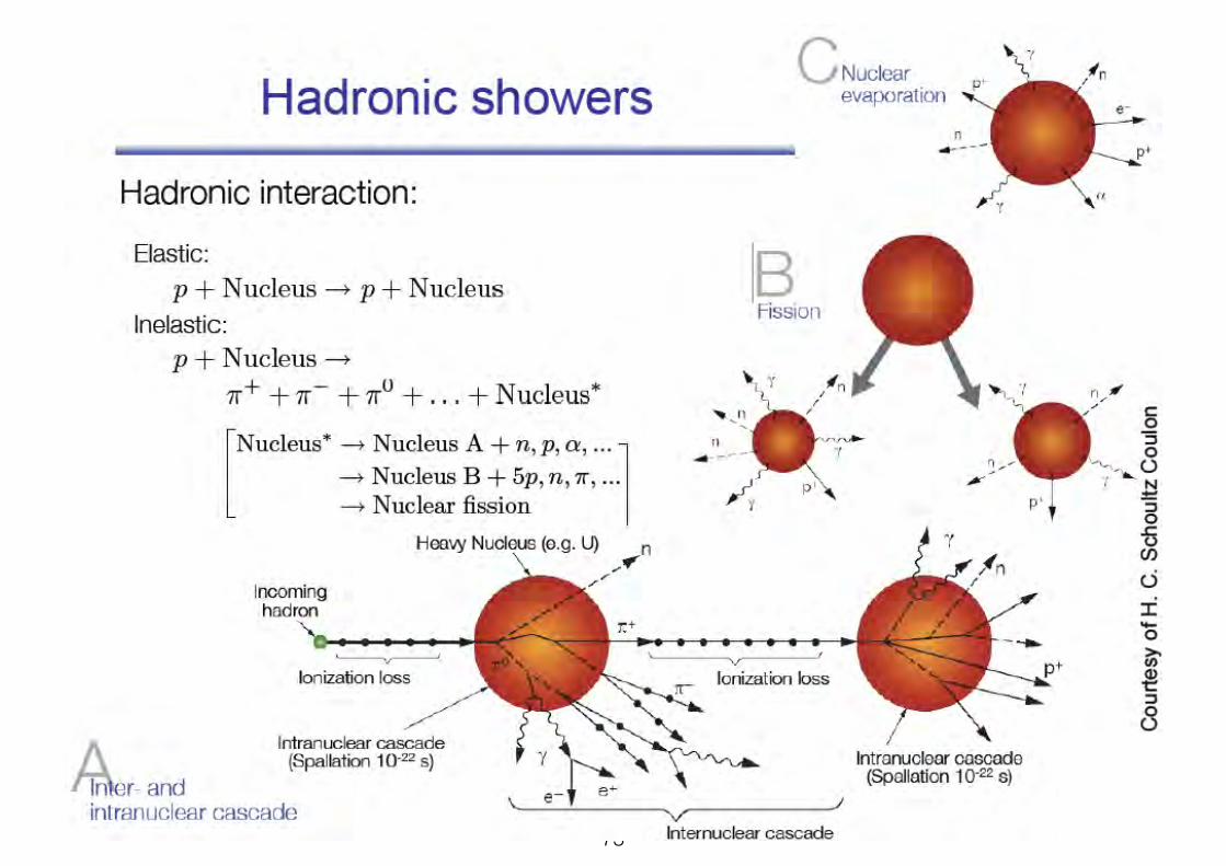
Hadronic interactions

• Dominant contribution to stopping of high energy hadrons

• Intranuclear cascade, leading to spallation

• Internuclear cascade, development of hadronic shower

40

Weak interaction

• Only relevant for neutrinos

• Charged and neutral currents

• Extremely small cross sections

41

Tracking and momentum measurement- measure track in magnetic field: determine momentum of charged particles

- identify secondary vertices: heavy flavor decays - separation of multiple interactions in single bunch crossing

42

Field geometries for 4π detectors (colliders)

• Solenoid: field lines parallel to beam direction

• The track of a charged particle represents a helix

• Needs magnetic flux return (iron)

43

• Toroid: field lines are circles in a plane perpendicular to beam direction

• The track of a charged particle represents a helix

• Needs magnetic flux return (iron)

ATLAS Toroid

44

Momentum determination

• Lorentz force = centrifugal force

• determine momentum from radius of curvature

• Charge from orientation of helix

45

Deflection in solenoidal field geometry

46

No field B-field ⊥ to projection

Tracking detectors

• We need to measure charged particle tracks in a magnetic field

• Requirements for a perfect tracking detector:

• Large volume coverage

• Position resolution in 3 dimensions

• Excellent position resolution

• Minimum perturbation of the particle’s momentum

• Can be operated at high rates

• Reasonable cost

47

partially contradicting requirements !!

Limitations to momentum resolution

• Momentum resolution limited:

• At high momentum by position resolution of the detector /strength of magnetic field

• At low momentum by multiple scattering

48

Consequences for momentum resolution

49

Gaseous detectors

50

Multi-Wire-Proportional Counters (MWPC)

51

Simple Proportional CounterGas Amplification near Anode

Multi-Wire Proportional CounterPosition resolution in 1 dimension

Multi-Wire Proportional CounterPosition resolution in 2 dimensionswith segmented cathode readout

Drift chamber• Problem with MWPC: need many wires in close distance to obtain good position resolution

• Expensive, due to large number of readout channels, each with amplifier, signal shaper and ADC

• Idea: measure drift time with respect to external start signal in addition to wire position

• Need additional field wires to avoid region with low electric field/long drift times

• Need additional Time-to-Digital converter (TDC) to measure the drive times

52

Planar and Cylindrical Drift Chambers

53

Example: Belle II Central Drift Chamber

• If all wires were parallel to beam axis, there would be no information on scattering angle

• Introduce “Stereo Layers”

54

BelleIICDC

Numberoflayers 56

Totalsensewires 14336

Gas He:C2H6

Sensewire W(ø30µm)

Fieldwire Al(ø120µm)

Time Projection Chamber (TPC)

55

TPC

56

ALICE has the largest TPC

57

New Technologies Micro-Pattern Gas Detectors

58

Gas Electron Multiplier (GEM)

59

Solid-State Detectors (mostly Silicon based)• Motivation:

• Precision tracking close to the interaction point with minimum perturbation of the particles

• Identify individual interactions in bunch crossing

60

• Identify heavy flavor decays from secondary vertices

Detector principle: diode with reverse bias

61

Position-sensitive detectors

62

Pixel Detectors

63

Example: Belle II experiment

65

Asymmetricbeams:Lorentz-boosttranslateslifetime

todecaylength

PrecisevertexingessentialtomeasureCPviolation

Silicon Vertex Dector

66

•SiliconVertexDetector(SVD)4layersofDSSDr=3.8cm,8.0cm,11.5cm,14cmL=60cm~1m2

•PixelDetector(PXD)2layersofDEPFETpixelsr=1.4cm,2.2cmL=12cm~0.027m2

DEPFET Pixel Sensor

67

• 768x250DEPFETPixels• 50x75μm2pixelpitch• 75μmthickness

Requires dedicated ASIC development

68

DHP(DataHandlingProcessor)Firstdatacompression

TSMC65nmSize4.0×3.2mm2StoresrawdataandpedestalsCommonmodeandpedestalcorrectionDatareduction(zerosuppression)TimingsignalgenerationRad.Hardproved(100Mrad)

UMC180nmSize5.0×3.2mm2

TIAandADCPedestalcompensationRad.Hardproved(20Mrad)

SwitcherBRowcontrol

AMS/IBMHVCMOS180nmSize3.6×1.5mm2

GateandClearsignalFastHVrampforClearRad.Hardproved(36Mrad)

Sensor

PXD

DCDB(DrainCurrentDigitizer)Analogfrontend

Calorimetry / Energy Measurement

69

Principle

70

Electromagnetic Shower

71

Longitudinal development of electromagnetic shower in copper

72

73

Comparison: Electromagnetic vs. Hadronic Showers

74

Hadronic Showers: Longitudinal development

75

Two types of calorimeters

76

Inorganic Scintillators

77

Organic Scintillators

78

Comparison

Inorganic scintillatorshigh light yield

[typical; εsc ≈ 0.13]

high density

[e.g. PBWO4: 8.3 g/cm3]

good energy resolution

complicated crystal growth

large temperature dependence

expensive

79

Organic scintillatorseasily shapedsmall temperature dependence pulse shape discrimination possible

cheap

lower light yield

[typical; εsc ≈ 0.03]

radiation damage

Example: Electromagnetic calorimeter of CMS

80

ATLAS LAr Calorimeter

81

Energy resolution: 3 contributions

82

CMS ECAL Energy Resolution

83

Particle Identification

84

If the momentum of a particle is known …

• then we need a second observable to identify the particle:

85

Example: LHCb Ring Imaging Cherenkov Detector (RICH)

86

Example: Transition radiation detetor (ALICE)

87

Putting everything together:

88

Onion Shell Principle

89

Example: CMS

90

Problem: many of the particles decay before they reach the detector

• How do we detect and identify short-lived particles?

• This depends critically on their lifetime and decay modes

• Consider as an example : Charm production in a e+e- collider

• At time 0, the reaction happens:

91

γ

e+

e−

q

q

e− e+

c

c

QCD

D0= (cu)

π− = (ud)

π+= (ud) D*+= (cd)

After 10-23 s : Hadronization

92

π− = (ud)

After 10-20 s: Hadronic Decays

93

D*+

π−

π+

π−

D0

π+

10-12 mD0

After 10-12 s: Weak Decays

• Our detector has not seen anything yet !

94

π−

π+

10-4 m

π+

π−

π−

K+

K−

π0

π+

γ

γ

D0

D0

We see this (after 10-8 s) !

π−

π+

1 m

π+

π−

π−

K+

K−π+

γ

γ

How can we reconstruct what happened ?• We need to measure all particles, which make it into our detectors as precisely as possible

• measure 3-momenta and angles• particle identification

• particle mass

• construct 4-momentum vectors • Next step:

• reconstruct decaying particles from

• invariant mass of their decay products• problem : which of the detected particles belong to a parent ?

• combinatorial background !• in case of a kinematically complete experiment

• from the missing mass of all other particles

• identify long-lived particles from their secondary decay vertices • works for week decays of particles with open strangeness, charm or beauty

96

Finally: modern detectors are heavy …. and big …. and expensive …

97