Determinacy for infinite games with more

than two players with preferences

Benedikt Lowe

Institute for Logic, Language and Computation, Universiteit van Amsterdam,

Plantage Muidergracht 24, 1018 TV Amsterdam, The Netherlands,

bloewe@science.uva.nl

Abstract

We discuss infinite zero-sum perfect-information games with more than two players.They are not determined in the traditional sense, but as soon as you fix a preferencefunction for the players and assume common knowledge of rationality and thispreference function among the players, you get determinacy for open and closedpayoff sets.

2000 AMS Mathematics Subject Classification. 91A06 91A10 03B99 03E99.

Keywords. Perfect Information Games, Coalitions, Preferences, Determinacy Ax-ioms, Common Knowledge, Rationality, Gale-Stewart Theorem, Labellings

1 Introduction

The theory of infinite two-player games is connected to the foundations ofmathematics. Statements like

“Every infinite two-player game with payoff set in the complexity class Γ isdetermined, i.e., one of the two players has a winning strategy”

1 The author was partially financed by NWO Grant B 62-584 in the project Verza-

melingstheoretische Modelvorming voor Oneindige Spelen van Imperfecte Infor-

matie and by DFG Travel Grant KON 192/2003 LO 834/4-1. He would like to ex-tend his gratitude towards Johan van Benthem (Amsterdam), Boudewijn de Bruin(Amsterdam), Balder ten Cate (Amsterdam), Derrick DuBose (Las Vegas NV),Philipp Rohde (Aachen), and Merlijn Sevenster (Amsterdam) for discussions onmany-player games.

are called determinacy axioms (for two-player games). When we sup-plement the standard (Zermelo-Fraenkel) axiom system for mathematics withdeterminacy axioms, we get a surprisingly fine calibration of very interestinglogical systems. Research in set theory from the 1960es to this day has shownthat many if not most of the interesting features of Higher Set Theory are con-nected to determinacy axioms for two-player games: they have connections toinfinitary combinatorics of large sets, to topology, to the theory of the realnumbers, and to many other areas of interest in foundations of mathematics.In general, determinacy axioms provide a rich theory of interesting features.(Cf. [Ka94, §§ 27–32].)

A natural but naıve approach would be to assume that if you increase thenumber of players and look at “determinacy axioms for three-player games”,the number of interesting features for set theory should also increase. It is well-known that the opposite is true: determinacy axioms of the above form forn-player games are only interesting if n = 2. In all other cases, they are trivial:If n = 1 they are all true, regardless of Γ, if n > 2 they are all false for almostall Γ (cf. Proposition 1). It turns out that if we want to give solution conceptsfor infinite many-player games, determinacy in the classical sense is not theright concept. Solutions that have been offered in the literature include givingup the notion of a pure strategy and moving to mixed strategies (cf. [Ga53]and [Br00]), and understanding many-player games as coalitional games. Inthis paper, we want to work with pure strategies and stay within the realm ofnon-cooperative perfect information games

In addition to common knowledge of rationality of all players involved, weneed to add fixed preferences of the players and common knowledge of thesepreferences. Then we are able to give solution concepts for many-player infinitegames (for payoffs of very restricted complexity, though).

The results of this paper are (for definitions, cf. Sections 2 and 3):

Let I be an arbitrary set of players, X an arbitrary set of moves, µ an arbitrarymoving function, Π an arbitrary total preference.

• If P is an open or closed payoff, then there is a rational labelling ℓ∗ suchthat one of the players has an SΠ

ℓ∗-winning strategy. (Theorems 8 and 9)• If 〈P, Π〉 is a exceptional least evil situation, then there is a rational labelling

ℓ∗ such that one of the players has an SΠℓ∗-winning strategy. (Theorem 13)

• If P is a payoff such that a finite set of players has a closed payoff set and therest of the players have an open payoff set, then there is a rational labellingℓ∗ such that one of the players has an SΠ

ℓ∗-winning strategy. (Theorem 19) 1

1 Theorem 13 is a special case of Theorem 19, but uses a different technique, andis thus interesting in its own right.

2

2 Definitions & Motivation

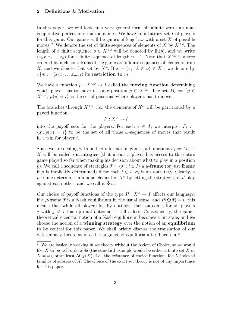
In this paper, we will look at a very general form of infinite zero-sum non-cooperative perfect information games. We have an arbitrary set I of playersfor this game. Our games will be games of length ω with a set X of possiblemoves. 2 We denote the set of finite sequences of elements of X by X<ω. Thelength of a finite sequence p ∈ X<ω will be denoted by lh(p), and we write〈x0x1x2 . . . xn〉 for a finite sequence of length n + 1. Note that X<ω is a treeordered by inclusion. Runs of the game are infinite sequences of elements fromX, and we denote that set by Xω. If x = 〈xk ; k ∈ ω〉 ∈ Xω, we denote byx↾m := 〈x0x1 . . . xm−1〉 its restriction to m.

We have a function µ : X<ω → I called the moving function determiningwhich player has to move in some position p ∈ X<ω. The set Mi := {p ∈X<ω ; µ(p) = i} is the set of positions where player i has to move.

The branches through X<ω, i.e., the elements of Xω will be partitioned by apayoff function

P : Xω → I

into the payoff sets for the players. For each i ∈ I, we interpret Pi :={x ; p(x) = i} to be the set of all those ω-sequences of moves that resultin a win for player i.

Since we are dealing with perfect information games, all functions σi := Mi →X will be called i-strategies (that means a player has access to the entiregame played so far when making his decision about what to play in a positionp). We call a sequence of strategies ~σ = 〈σi ; i ∈ I〉 a µ-frame (or just frameif µ is implicitly determined) if for each i ∈ I, σi is an i-strategy. Clearly, aµ-frame determines a unique element of Xω by letting the strategies in ~σ playagainst each other, and we call it z~σ.

Our choice of payoff functions of the type P : Xω → I affects our language:if a µ-frame ~σ is a Nash equilibrium in the usual sense, and P (z~σ) = i, thismeans that while all players locally optimize their outcome, for all playersj with j 6= i this optimal outcome is still a loss. Consequently, the game-theoretically central notion of a Nash equilibrium becomes a bit stale, and wechoose the notion of a winning strategy over the notion of an equilibriumto be central for this paper. We shall briefly discuss the translation of ourdeterminacy theorems into the language of equilibria after Theorem 8.

2 We are basically working in set theory without the Axiom of Choice, so we wouldlike X to be well-orderable (the standard example would be either a finite set X orX = ω), or at least ACX(X), i.e., the existence of choice functions for X-indexedfamilies of subsets of X. The choice of the exact set theory is not of any importancefor this paper.

3

A proper analysis of a class C of games would be something like the followingtheorem scheme:

For each payoff P ∈ C there is some player i ∈ I and an i-strategy σ suchthat for all relevant µ-frames ~τ with τi = σ, we have P (z~τ) = i.

The meaning of “relevant” has to be determined by the game analysis. In theclassical two-player case of set theory mentioned above, we have the degeneratecase where all strategies are relevant. This yields winning strategies: σ iswinning in the game with payoff P if for every µ-frame ~τ with τi = σ, we haveP (z~τ) = i. As usual, we call a payoff P determined if there is a winningi-strategy for some i ∈ I. For games with more than two players, winningstrategies might not always exist (Proposition 1).

For our classes Γ of payoffs we use the usual complexity classes of descriptiveset theory: Xω is endowed with a natural topology (the product topology ofthe discrete topology on X), and if X is finite or countable, this is a Polishspace. We have the usual pointclasses of open, closed, Borel, projective setson Xω, and for a pointclass Γ, we say that the payoff P : Xω → I is a Γ-payoffif for all i, Pi ∈ Γ. 3

Proposition 1 There is an open three-player game that is not determined.

Proof. Let X := {0, 1}, I = 3 = {0, 1, 2}, µ(p) := lh(p) mod 3 and

P0 := {x ; 〈010〉 ⊆ x or 〈011〉 ⊆ x},

P1 := {x ; 〈101〉 ⊆ x or 〈100〉 ⊆ x or 〈110〉 ⊆ x or 〈111〉 ⊆ x}, and

P2 := {x ; 〈000〉 ⊆ x or 〈001〉 ⊆ x},

as depicted in Figure 1 or (simplified) in Figure 2.

Clearly, the payoff sets are all open. Figure 2 shows that none of the threeplayers can have a winning strategy. q.e.d.

Consequently, for games with more than two players, we have to specify asmaller class of strategies as “relevant” in the sense of the above theoremscheme. This is well-known in game theory and led to studying many-playergames in terms of coalitions.

As mentioned, we shall stay within the non-cooperative paradigm, but addinformation about the preferences of the players and their rationality to the

3 Note that this usage is slightly different from the usage in the two-player case. Atwo-player game is normally called closed if the payoff for player I is a closed subsetof Xω (with no conditions on the payoff for player II).

4

?>=<89:;0

0jjjjjjjjj

uujjjjjjjjj 1TTTTTTTTT

))TTTTTTTTT

?>=<89:;1

0uu

uuu

zzuuuuu 1

IIII

I

$$IIII

I

?>=<89:;1

0uu

uuu

zzuuuuu 1

IIII

I

$$IIII

I

?>=<89:;2

0©©

¥¥©©1

66

½½66

?>=<89:;2

0©©

¥¥©©1

66

½½66

?>=<89:;2

0©©

¥¥©©1

66

½½66

?>=<89:;2

0©©

¥¥©©1

66

½½66

2 2 0 0 1 1 1 1

Fig. 1. The game graph of the game from Proposition 1. Round nodes with an i

represent opportunities for player i to move, square nodes denote the winner of agiven game path.

?>=<89:;0

0pppppppp

wwpppppppp 1KKKKKK

%%KKKKKK

?>=<89:;1

0¡¡

¡¡

¡¡¡¡¡ 1

>>>>

ÁÁ>>>

1

2 0

Fig. 2. Simplified version of Figure 1 with all irrelevant moves removed.

analysis. We shall presuppose full rationality of all players and common knowl-edge of that fact. This allows us to use the usual backwards induction tech-niques known from perfect information game analysis. 4 Assuming commonknowledge of rationality, we can restrict the set of relevant strategies; this willbe done when we define the notion of a 〈Π, ℓ〉-strategy in Section 3.

As an example, consider the game defined in Figure 1 and imagine that wehave the three players Jill (0), her husband Jeff (1), and an invited friend John(2). If Jill knows for sure that Jeff prefers her over John, she can exclude hisstrategy “play 0” from her considerations as irrelevant, and win by playing 0herself.

Note that this is not a coalition: there is no agreement between Jill and Jeff,there isn’t even a benefit for Jeff. It is just calculation of Jill, taking into ac-count predictions about the behaviour of her husband. Also note that playing0 can only guarantee Jill to win if she can be sure of both Jeff’s preference for

4 Cf. [Au95], [Bi88], [St96]. For a discussion of the role of common knowledge ofrationality for the backwards induction technique in terms of modal logic, cf. [dB∞].Note that the usual Gale-Stewart analysis for two players doesn’t need any rational-ity assumptions: the winning strategy constructed in the proof of the Gale-StewartTheorem will win against all players, including irrational ones. This is not true forour games anymore; we briefly discuss this at the end of this section.

5

her and Jeff’s rationality. If Jeff prefers Jill over John, but doesn’t properlyunderstand what’s going on in the game, he might play 0 and thus let Johnwin. (This type of the game will show up later in Section 7 as Evening at a

Couple.)

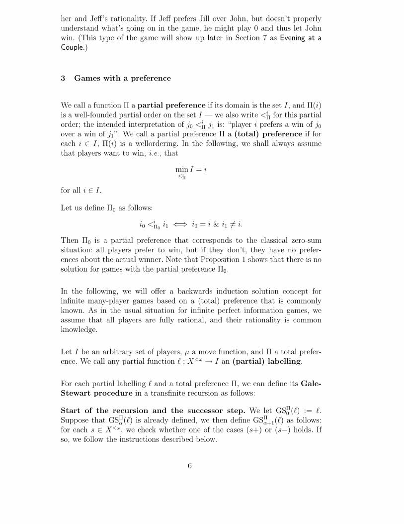
3 Games with a preference

We call a function Π a partial preference if its domain is the set I, and Π(i)is a well-founded partial order on the set I — we also write <i

Π for this partialorder; the intended interpretation of j0 <i

Π j1 is: “player i prefers a win of j0

over a win of j1”. We call a partial preference Π a (total) preference if foreach i ∈ I, Π(i) is a wellordering. In the following, we shall always assumethat players want to win, i.e., that

min<i

Π

I = i

for all i ∈ I.

Let us define Π0 as follows:

i0 <iΠ0

i1 ⇐⇒ i0 = i & i1 6= i.

Then Π0 is a partial preference that corresponds to the classical zero-sumsituation: all players prefer to win, but if they don’t, they have no prefer-ences about the actual winner. Note that Proposition 1 shows that there is nosolution for games with the partial preference Π0.

In the following, we will offer a backwards induction solution concept forinfinite many-player games based on a (total) preference that is commonlyknown. As in the usual situation for infinite perfect information games, weassume that all players are fully rational, and their rationality is commonknowledge.

Let I be an arbitrary set of players, µ a move function, and Π a total prefer-ence. We call any partial function ℓ : X<ω → I an (partial) labelling.

For each partial labelling ℓ and a total preference Π, we can define its Gale-Stewart procedure in a transfinite recursion as follows:

Start of the recursion and the successor step. We let GSΠ0 (ℓ) := ℓ.

Suppose that GSΠα (ℓ) is already defined, we then define GSΠ

α+1(ℓ) as follows:for each s ∈ X<ω, we check whether one of the cases (s+) or (s−) holds. Ifso, we follow the instructions described below.

6

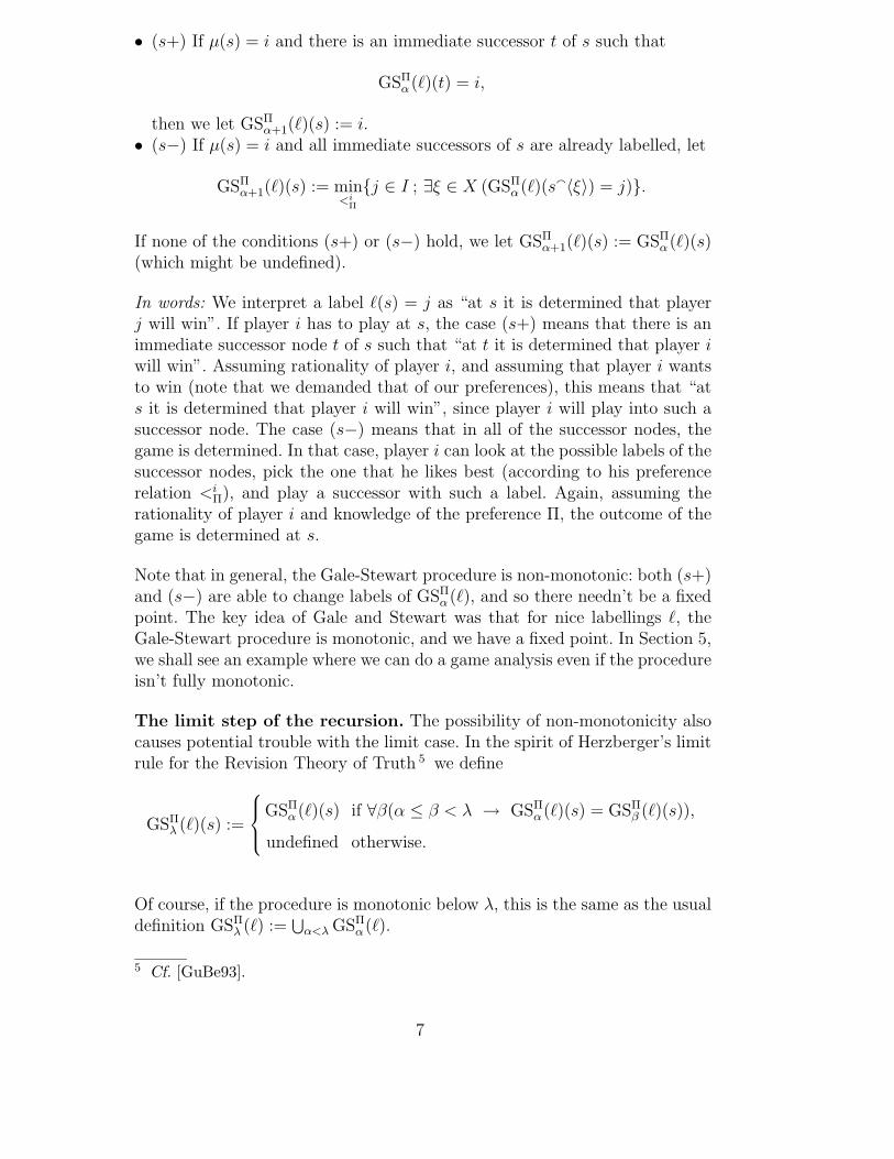
• (s+) If µ(s) = i and there is an immediate successor t of s such that

GSΠα (ℓ)(t) = i,

then we let GSΠα+1(ℓ)(s) := i.

• (s−) If µ(s) = i and all immediate successors of s are already labelled, let

GSΠα+1(ℓ)(s) := min

<iΠ

{j ∈ I ; ∃ξ ∈ X (GSΠα (ℓ)(sa〈ξ〉) = j)}.

If none of the conditions (s+) or (s−) hold, we let GSΠα+1(ℓ)(s) := GSΠ

α (ℓ)(s)(which might be undefined).

In words: We interpret a label ℓ(s) = j as “at s it is determined that playerj will win”. If player i has to play at s, the case (s+) means that there is animmediate successor node t of s such that “at t it is determined that player iwill win”. Assuming rationality of player i, and assuming that player i wantsto win (note that we demanded that of our preferences), this means that “ats it is determined that player i will win”, since player i will play into such asuccessor node. The case (s−) means that in all of the successor nodes, thegame is determined. In that case, player i can look at the possible labels of thesuccessor nodes, pick the one that he likes best (according to his preferencerelation <i

Π), and play a successor with such a label. Again, assuming therationality of player i and knowledge of the preference Π, the outcome of thegame is determined at s.

Note that in general, the Gale-Stewart procedure is non-monotonic: both (s+)and (s−) are able to change labels of GSΠ

α (ℓ), and so there needn’t be a fixedpoint. The key idea of Gale and Stewart was that for nice labellings ℓ, theGale-Stewart procedure is monotonic, and we have a fixed point. In Section 5,we shall see an example where we can do a game analysis even if the procedureisn’t fully monotonic.

The limit step of the recursion. The possibility of non-monotonicity alsocauses potential trouble with the limit case. In the spirit of Herzberger’s limitrule for the Revision Theory of Truth 5 we define

GSΠλ (ℓ)(s) :=

GSΠα (ℓ)(s) if ∀β(α ≤ β < λ → GSΠ

α (ℓ)(s) = GSΠβ (ℓ)(s)),

undefined otherwise.

Of course, if the procedure is monotonic below λ, this is the same as the usualdefinition GSΠ

λ (ℓ) :=⋃

α<λ GSΠα (ℓ).

5 Cf. [GuBe93].

7

If η is a fixed point of the Gale-Stewart construction, i.e., GSΠη (ℓ) = GSΠ

η+1(ℓ),

we call GSΠη (ℓ) the Gale-Stewart closure of ℓ relative to Π and denote

it by GSCΠ(ℓ). Regardless of whether the Gale-Stewart procedure has a fixedpoint or not, we call the least α such that GSΠ

α (ℓ)(s) is defined the index ofs.

Special properties of labellings. Let ℓ be a partial labelling, Π a totalpreference, and

〈GSΠα (ℓ) ; α ∈ Ord〉

be the Gale-Stewart procedure starting from ℓ.

We say that ℓ has the antichain property if for each infinite sequence〈sn ; n ∈ N〉 with sn+1 % sn there is some n such that sn ∈ dom(ℓ). Notethat this implies that dom(ℓ) is a maximal antichain in X<ω (and for thelabellings ℓ discussed in this paper, it is actually equivalent).

We say that ℓ has the Π-fixed point property if the Gale-Stewart procedurestarting from ℓ relative to Π has a fixed point, i.e., for some α, GSΠ

α (ℓ) =GSΠ

α+1(ℓ).

We say that ℓ has the Π-monotonicity property if for all α ∈ Ord, ifs ∈ dom(GSΠ

α (ℓ)), then

GSΠα (ℓ)(s) = GSΠ

α+1(ℓ)(s).

Obviously, this implies that the Gale-Stewart procedure is monotonic in theusual sense 6 , and we get a fixed point by the standard fixed point theoremfor monotonic operators:

Lemma 2 If ℓ has the Π-monotonicity property, it also has the Π-fixed pointproperty.

For some ℓ that has the Π-fixed point property, we say that it has the Π-totality property, if GSCΠ(ℓ) is a total function. We say that it has theΠ-root property if ∅ ∈ dom(GSCΠ(ℓ)).

Lemma 3 (Totality Lemma) If ℓ has the antichain property and the Π-monotonicity property, then it has the Π-totality property.

Proof. Suppose that s is not labelled by GSCΠ(ℓ). By (s−), all positionsthat have only labelled immediate successors are labelled in the Gale-Stewart

6 I.e., for all α < β, we have dom(GSΠα (ℓ)) ⊆ dom(GSΠ

β (ℓ)) and for s ∈

dom(GSΠα (ℓ)), we have GSΠ

α (ℓ)(s) = GSΠβ (ℓ)(s).

8

closure. Consequently, we can define an infinite sequence 〈sn ; n ∈ ω〉 withsn $ sn+1 starting from s such that for all n ∈ ω, sn /∈ dom(GSCΠ(ℓ)).

By the antichain property, there is some m such that sm ∈ dom(ℓ). But themonotonicity property of ℓ implies that dom(ℓ) ⊆ dom(GSCΠ(ℓ)) which is acontradiction. q.e.d.

Special properties of strategies. Let S be some class of strategies, and ℓbe some labelling. We call a frame ~τ = 〈τj ; j ∈ I〉 an S-frame if for all j ∈ I,we have τj ∈ S.

We call an i-strategy σ ℓ-S-consequent if for every S-frame ~τ such thatτi = σ, we have that

ℓ(z~τ↾n) = i

for all n ∈ ω. We call an i-strategy S-winning if for all S-frames ~τ and x := z~τ ,we have P (x) = i.

We call a strategy σ a 〈Π, ℓ〉-strategy if for all p with µ(p) = i, if ℓ(pa〈σ(p)〉) =k, then k is the <i

Π-least element of

{j ∈ I ; ∃x (ℓ(pa〈x〉) = j)}.

We denote the set of 〈Π, ℓ〉-strategies by SΠℓ .

Heuristics: We again assume that ℓ(s) = j is interpreted as “at s it is deter-mined that player j wins”. Suppose µ(p) = i; using his knowledge about ℓ,player i will be able to check his options at p by looking at the set

{ℓ(pa〈ξ〉) ; ξ ∈ X}.

Given the above interpretation of ℓ, the only rational choice for player i isto choose one of the successors that rank highest in his preference. A 〈Π, ℓ〉-strategy is one in which the player is required to behave rational in this way.

Lemma 4 Let ℓ be a labelling with the Π-totality property. Then there is aGSCΠ(ℓ)-SΠ

GSCΠ(ℓ)-consequent strategy.

Proof. We write ℓ∗ := GSCΠ(ℓ). By the Π-totality property, we have ℓ∗(∅) = ifor some i ∈ I. We define the following i-strategy σ: if µ(p) = i, play someξ such that pa〈ξ〉 has the <i

Π-least label among the immediate successors ofp. The labelling ℓ∗ is a total function and a fixed point of the Gale-Stewartprocedure, so for each node s, ℓ∗(s) must also be the label of at least oneimmediate successor of s.

Fix any SΠℓ∗-frame ~τ such that τi = σ, and let x := z~τ . We shall show that

ℓ∗(x↾n) = i for every n ∈ ω: Suppose it’s not, and let n + 1 be the least

9

counterexample (thus ℓ∗(x↾n) = i and ℓ∗(x↾n + 1) 6= i). By the above remark,we know that there is some immediate successor p of x↾n such that ℓ∗(p) = i.

Thus, by the choice of σ, we know that µ(x↾n) = j 6= i because player i wouldhave chosen to play p instead of x↾n + 1. But now by (x↾n−), we have

i = min<

j

Π

{k ∈ I ; ∃ξ ∈ X (ℓ∗(sa〈ξ〉) = k)},

yet τj(x↾n) = x(n) with i <jΠ ℓ∗(x↾n + 1). Thus τj is not a 〈Π, ℓ∗〉-strategy.

Contradiction. q.e.d.

4 Open and Closed Preference Games

4.1 Open Payoffs

Now let I be an arbitrary set of players, µ a move function, Π a total preference,and P an open payoff.

We define

Si := {p ∈ X<ω ; ∀x (p ⊆ x implies P (x) = i)}

to be the set of positions at which player i has won, and set

ℓ(p) := i : ⇐⇒ p ∈ Si.

We call a labelling ℓ an open labelling if there is an open payoff P as above.

Lemma 5 Every open labelling has the antichain property.

Proof. Obvious. q.e.d.

Lemma 6 Every open labelling has the Π-monotonicity property (for arbi-trary preferences Π).

Proof. Let 〈GSΠℓ (α) ; α ∈ Ord〉 be the Gale-Stewart procedure derived from

ℓ. We prove the claim by induction on the index of s. Suppose s is a coun-terexample of minimal index, so GSΠ

α (ℓ)(s) = i 6= j = GSΠα+1(ℓ)(s). Take α to

be minimal among those as well.

Case 1. The index is β + 1, and s was labelled by (s+). Then there is someimmediate successor t with strictly lower index such that GSΠ

β (ℓ)(t) = i. By

minimality, GSΠα (ℓ)(t) = i, so (s+) is applied in the construction of GSΠ

α+1(ℓ),hence GSΠ

α+1(ℓ)(s) = i. Contradiction.

10

Case 2. The index is β + 1, and s was labelled by (s−). Then all immediatesuccessors t have strictly lower index, and thus by minimality, their labels arefixed. So (s−) is applied in the construction of GSΠ

α+1(ℓ), hence GSΠα+1(ℓ)(s) =

i. Contradiction.

Case 3. Suppose that the index of s is 0. In that case, all successors (notonly immediate) are i-labelled with index 0, so by induction GSΠ

α+1(ℓ)(s) = i.Contradiction. q.e.d.

Corollary 7 Every open labelling has the Π-totality property (for arbitrarypreferences Π).

Proof. From Lemmas 5 and 6 via the Totality Lemma 3. q.e.d.

Theorem 8 Let I be an arbitrary set of players, µ an arbitrary move function,P an open payoff, ℓ the open labelling derived from P , ℓ∗ its Gale-Stewartclosure, and Π a (total) preference. Then there is an i ∈ I and a SΠ

ℓ∗-winningstrategy σ for player i.

Proof. By Corollary 7, GSCΠ(ℓ) is total, so let GSCΠ(ℓ)(∅) = i. Using (theproof of) Lemma 4, we get a GSCΠ(ℓ)-SΠ

ℓ∗-consequent strategy σ for player i.Let ~τ be an arbitrary SΠ

ℓ∗-frame with τi = σ, and let x := z~τ . We have thatfor every n ∈ ω, GSCΠ(ℓ)(x↾n) = i.

Lemma 5 gives us some m such that x↾m ∈ dom(ℓ), and Lemma 6 yields thatℓ(x↾m) = GSCΠ(ℓ)(x↾m) = i, i.e., x ∈ Si, and thus P (x) = i. q.e.d.

In terms of determinacy axioms, the analysis of this section yields a many-player determinacy statement:

For open payoffs and arbitrary sets of players, if we fix a (total) preferenceΠ, then there is a Π-winning strategy for one of the players.

Let us rephrase this in terms of equilibria: If we restrict the class of relevantstrategies to the strategies in SΠ

ℓ∗ , then Theorem 8 gives us a large set of verystrong equilibria: Each frame ~τ such that τi = σ is an equilibrium since none ofthe players can increase his payoff while playing a strategy in SΠ

ℓ∗ ; the playersj 6= i necessarily lose against σ.

4.2 Closed Payoffs

If I is finite and P is closed, then all sets Pi are also open, and Theorem 8 canbe applied. If I is infinite, it could be that the payoff sets are closed but not

11

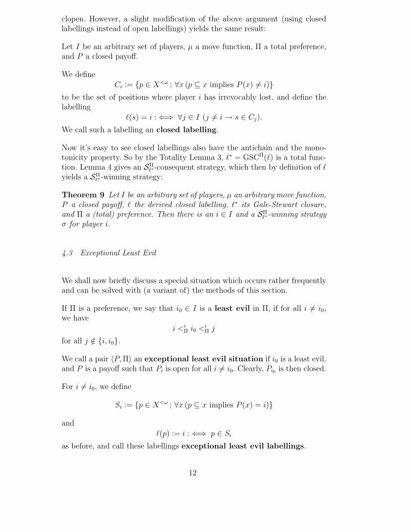
clopen. However, a slight modification of the above argument (using closedlabellings instead of open labellings) yields the same result:

Let I be an arbitrary set of players, µ a move function, Π a total preference,and P a closed payoff.

We define

Ci := {p ∈ X<ω ; ∀x (p ⊆ x implies P (x) 6= i)}

to be the set of positions where player i has irrevocably lost, and define thelabelling

ℓ(s) = i : ⇐⇒ ∀j ∈ I (j 6= i → s ∈ Cj).

We call such a labelling an closed labelling.

Now it’s easy to see closed labellings also have the antichain and the mono-tonicity property. So by the Totality Lemma 3, ℓ∗ = GSCΠ(ℓ) is a total func-tion. Lemma 4 gives an SΠ

ℓ∗-consequent strategy, which then by definition of ℓyields a SΠ

ℓ∗-winning strategy:

Theorem 9 Let I be an arbitrary set of players, µ an arbitrary move function,P a closed payoff, ℓ the derived closed labelling, ℓ∗ its Gale-Stewart closure,and Π a (total) preference. Then there is an i ∈ I and a SΠ

ℓ∗-winning strategyσ for player i.

4.3 Exceptional Least Evil

We shall now briefly discuss a special situation which occurs rather frequentlyand can be solved with (a variant of) the methods of this section.

If Π is a preference, we say that i0 ∈ I is a least evil in Π, if for all i 6= i0,we have

i <iΠ i0 <i

Π j

for all j /∈ {i, i0}.

We call a pair 〈P, Π〉 an exceptional least evil situation if i0 is a least evil,and P is a payoff such that Pi is open for all i 6= i0. Clearly, Pi0 is then closed.

For i 6= i0, we define

Si := {p ∈ X<ω ; ∀x (p ⊆ x implies P (x) = i)}

and

ℓ(p) := i : ⇐⇒ p ∈ Si

as before, and call these labellings exceptional least evil labellings.

12

We get analogues of Lemmas 5 and 6:

Lemma 10 If 〈P, Π〉 is an exceptional least evil situation and ℓ the derivedlabelling, then for every x ∈ Xω, we have

• either there is some n such that x↾n ∈ dom(ℓ),• or P (x) = i0.

Lemma 11 If 〈P, Π〉 is an exceptional least evil situation, then its derivedlabelling has the Π-monotonicity property.

Consequently, exceptional least evil labellings have the Π-fixed point property.However, the Gale-Stewart closure needn’t be total this time as they do nothave the antichain property. We define

ℓ∗(s) =

GSCΠℓ (s) if s ∈ dom(GSCΠ(ℓ)), and

i0 otherwise.

If s /∈ dom(GSCΠ(ℓ)), we say that the index of s is 0.

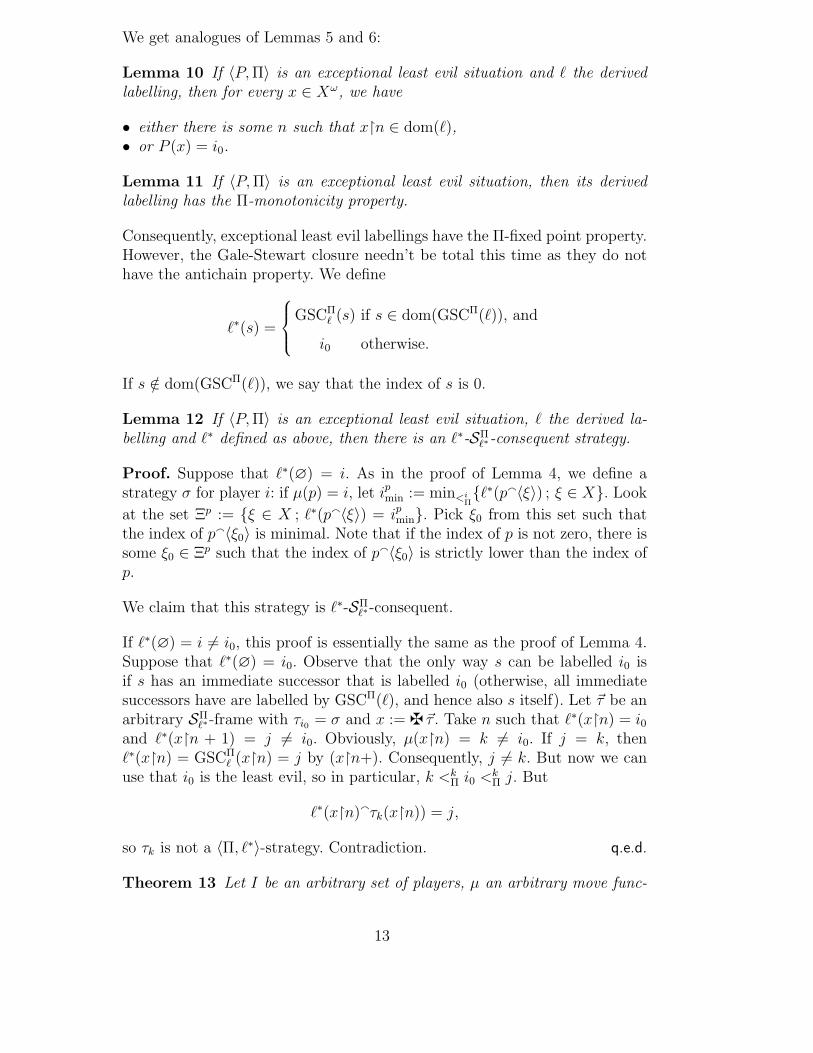
Lemma 12 If 〈P, Π〉 is an exceptional least evil situation, ℓ the derived la-belling and ℓ∗ defined as above, then there is an ℓ∗-SΠ

ℓ∗-consequent strategy.

Proof. Suppose that ℓ∗(∅) = i. As in the proof of Lemma 4, we define astrategy σ for player i: if µ(p) = i, let ipmin := min<i

Π

{ℓ∗(pa〈ξ〉) ; ξ ∈ X}. Look

at the set Ξp := {ξ ∈ X ; ℓ∗(pa〈ξ〉) = ipmin}. Pick ξ0 from this set such thatthe index of pa〈ξ0〉 is minimal. Note that if the index of p is not zero, there issome ξ0 ∈ Ξp such that the index of pa〈ξ0〉 is strictly lower than the index ofp.

We claim that this strategy is ℓ∗-SΠℓ∗-consequent.

If ℓ∗(∅) = i 6= i0, this proof is essentially the same as the proof of Lemma 4.Suppose that ℓ∗(∅) = i0. Observe that the only way s can be labelled i0 isif s has an immediate successor that is labelled i0 (otherwise, all immediatesuccessors have are labelled by GSCΠ(ℓ), and hence also s itself). Let ~τ be anarbitrary SΠ

ℓ∗-frame with τi0 = σ and x := z~τ . Take n such that ℓ∗(x↾n) = i0and ℓ∗(x↾n + 1) = j 6= i0. Obviously, µ(x↾n) = k 6= i0. If j = k, thenℓ∗(x↾n) = GSCΠ

ℓ (x↾n) = j by (x↾n+). Consequently, j 6= k. But now we canuse that i0 is the least evil, so in particular, k <k

Π i0 <kΠ j. But

ℓ∗(x↾n)aτk(x↾n)) = j,

so τk is not a 〈Π, ℓ∗〉-strategy. Contradiction. q.e.d.

Theorem 13 Let I be an arbitrary set of players, µ an arbitrary move func-

13

tion, 〈P, Π〉 an exceptional least evil situation, ℓ the derived labelling, and ℓ∗

as defined above. There is an i ∈ I and an SΠℓ∗-winning strategy σ for player i.

Proof. The strategy σ as defined in the proof of Lemma 12 will be the SΠℓ∗-

winning strategy. Remember that σ always plays into positions of strictly lowerindex (unless the index is 0). Let ~τ be a SΠ

ℓ∗-frame with τi = σ and x := z~τ .Then by Lemma 12, ℓ∗(x↾n) = i for all n ∈ ω.

We are left to show that P (x) = i. By Lemma 10, we know that this is thecase if i = i0. So let i 6= i0.

Note that if µ(x↾n) = j 6= i, then it was either already i-labelled in ℓ or itwas i-labelled by (x↾n−), so all immediate successors have strictly lower indexthan x↾n. This together with the choice of σ says that the sequence of indicesof x↾n is a decreasing sequence of ordinals. Hence it must eventually reach 0,which means that x↾n ∈ Si for some n ∈ ω. q.e.d.

The fact that the index function needs to be used in order to define a winningstrategy in this case is no coincidence: as opposed to games in which all payoffsare open or all payoffs are closed, the games with an exceptional least evilcontain for example all so-called combinatorial games (games with counterson graphs; the last player to move the counter wins, if the counter is movedinfinitely many times, it’s a draw). That labelling functions for combinatorialgames need transfinite ordinal values to describe winning strategies has beendiscussed in [FrRa01].

5 Mixed Labels

The analysis of Section 4, in particular Section 4.3 covers quite a lot: Theusual open and closed two-player games (i.e., P0 open and P1 closed, or viceversa) are an instance of an exceptional least evil (the closed player is theexception); also all games with open payoffs and a draw are instances of anexceptional least evil (as mentioned, the combinatorial games on graphs areexamples of these).

But there are other situations that the analysis of Section 4.3 cannot dealwith, for example a closed player who is not a least evil, or two closed and oneopen players.

For these situation we need to mix open and closed labellings, and give upmonotonicity.

Let I be a set of players, µ a move function and P be a payoff such that Pi

14

is either open or closed for all i ∈ I. We shall call such a payoff function amixed payoff. Let Iopen ∪ Iclosed be a disjoint partition of I such that for alli ∈ Iopen, Pi is open and for all i ∈ Iclosed, Pi is closed. Assume in additionthat Iclosed is finite (this is used in the proof of Lemma 14).

We are now joining the ideas of open and closed labellings. For each i ∈ Iclosed,let

Ci := {p ∈ X<ω ; ∀x (p ⊆ x implies P (x) 6= i)}

be the set of positions where player i has irrevocably lost, and for each i ∈ Iopen,let

Si := {p ∈ X<ω ; ∀x (p ⊆ x implies P (x) = i)}

be the set of positions at which player i has won.

We define the following mixed labelling:

ℓ(s) :=

i ∈ Iopen if s ∈ Si,

j ∈ Iclosed if s /∈⋃

{Si ; i ∈ Iopen} ∪⋃

{Ck ; k ∈ Iclosed, k 6= j}.

Labellings derived from a mixed payoff function in this way are called mixedlabellings.

Lemma 14 Every mixed labelling has the antichain property.

Proof. Let x ∈ Xω, and let P (x) = i. If i ∈ Iopen, then there is some n suchthat x↾n ∈ Si.

If i ∈ Iclosed, then for each j ∈ Iclosed such that j 6= i there is some naturalnumber nj with x↾nj ∈ Cj. Let n := max{nj ; j ∈ Iclosed, j 6= i} (note thatthis exists because Iclosed is finite). Then ℓ(x↾n) = i. q.e.d.

If now 〈GSΠα (ℓ) ; α ∈ Ord〉 is the Gale-Stewart procedure starting from a mixed

labelling ℓ, it is not necessarily monotonic anymore:

For example, if I = X = {0, 1}, µ(∅) = 0, P0 := {x ; x(0) = 0}, then ℓ(∅) = 1and ℓ(〈0〉) = 0. Then (∅+) gives GSΠ

1 (ℓ)(∅) = 0 6= 1 = GSΠ0 (ℓ)(∅). We call

such a situation, i.e., a pair 〈s, α〉 such that

GSΠα (ℓ)(s) = i 6= j = GSΠ

α+1(ℓ)(s)

an overwriting instance (for ℓ).

Lemma 15 If ℓ is a mixed labelling and 〈s, α〉 is an overwriting instance with

GSΠα (ℓ)(s) = i 6= j = GSΠ

α+1(ℓ)(s),

then i ∈ Iclosed, j ∈ Iopen, and GSΠα (ℓ)(s) = ℓ(s).

15

Proof. We prove this by induction on the index of s. Suppose s is a coun-terexample of minimal index. Take α to be minimal among those as well.

Case 1., Case 2. and Case 3. from the proof of Lemma 6, show that theindex of s must be 0, and that i cannot be an open label, so i ∈ Iclosed. Bydefinition of ℓ, we know that

Iclosed ∩ {ℓ(t) ; t ⊇ s} = {i}.

So by induction, GSΠα (ℓ)(t) ∈ Iopen∪{i} for all successors t ⊇ s. Consequently,

if GSΠα+1(ℓ)(s) = j 6= i, then j ∈ Iopen. But now the minimal choice of α gives

ℓ(s) = GSΠα (ℓ)(s) by induction, so s was no counterexample. q.e.d.

Corollary 16 If ℓ is a mixed labelling and s ∈ X<ω, then there is at mostone α such that GSΠ

α (ℓ)(s) 6= GSΠα+1(ℓ)(s).

Proof. By Lemma 15, if GSΠα (ℓ)(s) 6= GSΠ

α+1(ℓ)(s), then GSΠα (ℓ)(s) ∈ Iclosed

and GSΠα+1(ℓ)(s) ∈ Iopen. But now again by Lemma 15 this means that for no

β > α, we can have GSΠβ (ℓ)(s) 6= GSΠ

β+1(ℓ)(s). q.e.d.

Lemma 17 Every mixed labelling has the Π-fixed point property (for arbitraryΠ).

Proof. By Corollary 16, there is only a set of overwriting instances (in fact,the cardinality of the set is at most κ := Card(X<ω). Let

Σ := sup{α + 1 ; 〈s, α〉 is an overwriting instance for some s ∈ X<ω}.

Then after Σ, the Gale-Stewart procedure is fully monotonic, and hence hasa fixed point by the usual fixed point theorem. q.e.d.

Lemma 18 Every mixed labelling has the Π-totality property (for arbitraryΠ).

Proof. We know by Lemma 14 that ℓ has the antichain property. Note thatthe proof of the Totality Lemma 3 doesn’t really need the full Π-monotonicityproperty but only

s ∈ dom(ℓ) → s ∈ dom(GSCΠ(ℓ)) (†)

which is a consequence of Corollary 16. q.e.d.

Theorem 19 Let I = Iopen ∪ Iclosed be an arbitrary set of players where Iclosed

is finite, µ an arbitrary move function, P a payoff such that Pi is open fori ∈ Iopen and Pi is closed for i ∈ Iclosed, ℓ the derived mixed labelling, and ℓ∗

its Gale-Stewart closure (which exists by Lemma 17). Then there is an i ∈ Iand an SΠ

ℓ∗-winning strategy σ for player i.

16

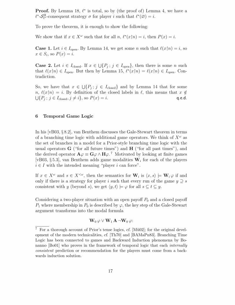
Proof. By Lemma 18, ℓ∗ is total, so by (the proof of) Lemma 4, we have aℓ∗-SΠ

ℓ∗-consequent strategy σ for player i such that ℓ∗(∅) = i.

To prove the theorem, it is enough to show the following:

We show that if x ∈ Xω such that for all n, ℓ∗(x↾n) = i, then P (x) = i.

Case 1. Let i ∈ Iopen. By Lemma 14, we get some n such that ℓ(x↾n) = i, sox ∈ Si, so P (x) = i.

Case 2. Let i ∈ Iclosed. If x ∈⋃

{Pj ; j ∈ Iopen}, then there is some n suchthat ℓ(x↾n) ∈ Iopen. But then by Lemma 15, ℓ∗(x↾n) = ℓ(x↾n) ∈ Iopen. Con-tradiction.

So, we have that x ∈⋃

{Pj ; j ∈ Iclosed} and by Lemma 14 that for somen, ℓ(x↾n) = i. By definition of the closed labels in ℓ, this means that x /∈⋃

{Pj ; j ∈ Iclosed, j 6= i}, so P (x) = i. q.e.d.

6 Temporal Game Logic

In his [vB03, § 8.2], van Benthem discusses the Gale-Stewart theorem in termsof a branching time logic with additional game operators. We think of Xω asthe set of branches in a model for a Prior-style branching time logic with theusual operators G (“for all future times”) and H (“for all past times”), andthe derived operator Aϕ ≡ Gϕ ∧Hϕ. 7 Motivated by looking at finite games[vB03, § 5.3], van Benthem adds game modalities Wi for each of the playersi ∈ I with the intended meaning “player i can force”.

If x ∈ Xω and s ∈ X<ω, then the semantics for Wi is 〈x, s〉 |= Wi ϕ if andonly if there is a strategy for player i such that every run of the game y ⊇ sconsistent with y (beyond s), we get 〈y, t〉 |= ϕ for all s ⊆ t ⊆ y.

Considering a two-player situation with an open payoff P0 and a closed payoffP1 where membership in P0 is described by ϕ, the key step of the Gale-Stewartargument transforms into the modal formula

W0 ϕ ∨ W1 A¬W0 ϕ:

7 For a thorough account of Prior’s tense logics, cf. [Mu02]; for the original devel-opment of the modern technicalities, cf. [Th70] and [BAMaPn83]. Branching TimeLogic has been connected to games and Backward Induction phenomena by Bo-nanno [Bo01] who proves in the framework of temporal logic that each internally

consistent prediction or recommendation for the players must come from a back-wards induction solution.

17

either player 0 can force the outcome into P0 or player 1 can make sure thatplayer 0 can never force the outcome into P0.

8

This is exactly the claim of Lemma 12, and if we are in the case of the secondalternative (W1 A¬W0 ϕ), we use the fact that P1 is closed to show that thisis enough to prove that the outcome is in P1.

Of course, when we move to more general formulas ϕ of temporal logic, theWeak Determinacy formula might not be enough to prove determinacy any-more, and also the provability of the Weak Determinacy formula might dependon the system we’re working in.

In the cases of open payoffs, closed payoffs and mixed payoffs with the non-monotone analysis of Section 5, the explication in a temporal game logic termbecomes even simpler and is identical with the statement of determinacy:

∨

i∈I

Wi ϕi

where ϕi is a formula describing membership in Pi.9 The case of the Excep-

tional Least Evil reverts to the Gale-Stewart situation and gives

∨

i6=i0

Wi ϕi ∨ Wi0 A∧

i6=i0

¬Wi ϕi.

7 Games with three players

We now give some examples of games solved by the solution concepts by openlabellings and mixed labellings given in Sections 4 and 5.

For this let’s look a bit more closely at three-player games with preferences.Up to renaming of the players, there are only two different three-player gameswith total preferences, we call them Evening at a Married Ex and Love Triangle

(depicted in Figure 3). In our pictures of the preferences, an arrow from i toj means “i prefers j over k” (where {i, j, k} = {0, 1, 2}).

Of course, the solution concept presented in Theorem 19 gives us optimalstrategies for some player in these games if the payoffs are open and/or closed.

8 This is called Weak Determinacy by van Benthem [vB03].9 If I is infinite, we either need to interpret the disjunction

∨

as a quantifier withthe obvious semantics or move to an infinitary logic.

18

0 ** 1jj 0 ** 1

ww2

VV

2

VV

Fig. 3. Evening at a Married Ex and Love Triangle

For three players, if Π(i) is not a wellordering, it is necessarily of the formi <i

Π j, k where j and k are in no particular ordering. So if Π is not a totalpreference, then either one, two, or all three of the relations <i

Π are of thisform. There are (up to renaming) three cases with two wellorderings, and onecase each with one and zero wellorderings. They are depicted in Figures 4 and5.

0 ** 1

ww

0 ** 1jj 0

''

1

ww2 2 2

Fig. 4. Beatrice’s Revenge, Evening at a Couple, and Least Evil

In general, there are no solution concepts for partial preferences. Of course,Hobbes is just the case of full non-cooperation and as mentioned in Proposition1, there is no solution for this situation. A notable exception is Least Evil: In thecase where the least evil itself doesn’t move (i.e., M2 = ∅), the “ExceptionalLeast Evil” analysis of Section 4.3 is a solution.

Let us briefly describe the different situations by examples:

Love Triangle. This situation is truly pseudo-Shakespearean: Beatrice (0) is thefiancee of the poor but handsome Captain Antonio (1). She recently startedto question her fiance’s character. Faking a family emergency, she pretendsto go to the countryside while dressing as a rich wine merchant to check onAntonio’s behaviour. Alas, her suspicions prove to be correct: as soon as sheapparently leaves town, Antonio starts a liaison with the beautiful Cressida(2). Beatrice in the role the wine merchant is intent on confronting Antoniowith his deeds and invites Antonio and Cressida to play an infinite three-player game. Now the treacherous heart of Cressida abandons poor Antoniofor the rich wine merchant (0 <2

Π 1) while the good-hearted Beatrice is fullof pity for Antonio seeing him so deceived by Cressida (1 <0

Π 2). Antonio, ofcourse, doesn’t evaluate the situation correctly: he doesn’t recognize Beatrice,and although he realizes that Cressida has abandoned him, he tries to win herback by preferring her in the game (2 <1

Π 0).

Beatrice’s Revenge. In the situation of Love Triangle, Beatrice realizes thatAntonio is an idiot. Even though Cressida shamelessly flirts with the rich winemerchant, Antonio gazes in benumbed infatuation at her. Suddenly, Beatricerealizes that this buffoon of a Captain doesn’t deserve her compassion, and

19

she gives up favouring Antonio over Cressida.

Evening at a Couple. John (2) visits his friends, the married couple Jeff (1) andJill (0) at home. They decide to kill some time by playing an infinite three-player game. Although Jeff and Jill are good sports and try to play the gamewithout prejudice, subconsciously, they prefer their marital partner over John(0 <1

Π 2, 1 <0Π 2). John knows that pretty well, and realizes that it makes no

difference whether Jeff or Jill wins.

Evening at a Married Ex. We are in the situation of Evening at a Couple butwith an added twist: Jill was the girlfriend of John for a long time while theywere in graduate school, and (not unbeknownst to Jill) John is still in lovewith her (0 <2

Π 1).

Least Evil. We are in a Mathematics Department with Professors Smith (0),Johnson (1) and Williams (2) eligible to become the new Chair. 10 Smith andMiller are ambitious administrators and know that the only way to becomeDean of the Faculty of Sciences is to become Department Chair. Of course,they also know that if the other one becomes Chair, he will probably usehis chance to become Dean, and the position of the Dean will be blocked forat least five if not ten years. Williams is not ambitious at all – both Smithand Miller realize that if Williams were to become Chair, he would never aimat the office of Dean (2 <0

Π 1, 2 <1Π 0). As laid out in the bylaws of the

Mathematics Department, Smith, Johnson and Williams have to engage in aninfinite three-player game to determine the next Chair.

Of course, Least Evil is a very common situation. As mentioned, if M2 = ∅,we end up with a two-player game with draw.

0 ** 1 0 1

2 2

Fig. 5. Sidekick and Hobbes

Sidekick. Luigi (1) and Paolo (2), two mafia bosses meet to deal with eachother, and Luigi brought his faithful follower Giacomo (0). They play an infi-nite game, and whoever wins the game will become Overlord of Crime. Each ofthem is given a chance of winning that title, but what about the consequencesof losing? Clearly, if Paolo wins, he will most probably kill both Luigi and

10 To stifle any discussions about the choice of these surnames: According to at leastone poll, the most common surnames in the United States in the year 2000 were (inthat order): Smith, Johnson, Williams, Jones, Brown, Davis, Miller, Wilson, Moore,Taylor.

20

Giacomo to thwart any opposition forming around them; similarly, he can besure to be killed for the same reason by either of the others if they win. Luigihas humiliated Giacomo over many years, so Luigi can’t be sure of his futureif Giacomo wins. The only one who has a preference is Giacomo: if Luigi wins,he will stay alive –and continue to be humiliated by Luigi–; if Paolo wins, he’lldie (1 <0

Π 2).

Hobbes. In this three-player game there are no preferences except that allplayers wish to win, and if they don’t, they don’t care who does. This type ofgame is played in the Hobbesian Natural Condition of Mankind :

If any two men desire the same thing, which nevertheless they cannot bothenjoy, they become enemies; and in the way to their end (which is principallytheir own conservation, and sometimes their delectation only) endeavour todestroy or subdue one another. ... Men have no pleasure (but on the contrarya great deal of grief) in keeping company where there is no power able tooverawe them all. ... It is manifest that during the time men live without acommon power to keep them all in awe, they are in that condition which iscalled war; and such a war as is of every man against every man (Hobbes,Leviathan XIII).

As pointed out, this situation is the fully non-cooperative situation describedin Proposition 1, and thus Π-preference determinacy cannot offer a solutionconcept for these games.

8 Conclusion

We gave solution concepts for infinite multi-player games with the strongestcommon knowledge assumptions and for very simple payoffs. Of course, thereare many directions to discuss variations of these themes:

More complicated payoffs. As can be made explicit, ∆02 payoffs still allow

combinatorial labellings, thus it is possible to give a version of backwardsinduction. That suggests that the arguments from this paper could possiblybe extended to ∆0

2 payoffs.

Furthermore, almost all determinacy proofs in set theory go back to opendeterminacy. The key notion here is the tree representation of more compli-cated sets by κ-homogeneous trees (cf. [Ka94, § 32]). Winning a game on theclosed payoff set given by the tree can be transformed into winning the origi-nal game. Can we give homogeneous tree version for many-players games withmore complicated payoffs (e.g., assuming that the players have agreed to beplaying according to one fixed homogeneous tree before the game)?

21

Other knowledge assumptions. Consider the following version of Love

Triangle where Antonio is even less observant: He doesn’t recognize Beatrice,but moreover he also doesn’t realize that Cressida has abandoned him, so inevaluating the game tree, he will evaluate the positions as if 1 <2

Π 0 instead of(the correct) 0 <2

Π 1. Assuming that Beatrice and Cressida know about thiserror in judgement of Antonio’s, can we give a solution of the game? Whatif we allow Antonio to change his mind (and thus the labelling of the gametree in his mind) as soon as he sees that Cressida has betrayed him? 11 Thisnecessarily leads to dynamic models of these games similar to dynamic modelsfor epistemic solutions of finite games (cf. [vB01]).

Proof-theoretic analysis & more non-monotonicity. The existence ofwinning strategies has been analyzed proof-theoretically in terms of weak sys-tems of second-order arithmetic. 12

Deleting and overwriting of labels for games as in the analysis of mixed la-bellings occurs in some proof-theoretic analyses of subsystems of second-ordernumber theory [Mo03], and in full generality might be connected to gamescorresponding to the proof-theoretic strength of Gupta-Belnap revision the-ory. 13 Thus extending the ideas of Section 5 to labellings with the antichainproperty but with truly non-monotonic Gale-Stewart procedures that need tobe analysed as revision sequences is an interesting approach to game-theoreticanalyses of Revision Theory.

References

[Au95] Robert J.Aumann, Backward Induction and CommonKnowledge of Rationality, Games and Economic Behavior 8(1995), p. 6–19

[BAMaPn83] Mordechai Ben-Ari, Zohar Manna, Amir Pnueli, The temporallogic of branching time, Acta Informatica 20 (1983), p. 207–226

[Bi88] Ken Binmore, Modelling Rational Players. Part II, Economics

and Philosophy 4 (1988), p. 9-55

[Bo01] Giacomo Bonanno, Branching Time Logic, Perfect InformationGames and Backward Induction, Games and Economic

Behavior 36 (2001), p. 57–73

11 For finite games, this has been considered by Kreps et al. in [Kr+82].12 Cf. [Ta90], [Ta91], [Mo03], and in particular the textbook [Si99].13 Cf. [KuLoMoWe∞] for a discussion of the strength of Revision Theory and of theconnections between Revision Theory and games.

22

[Br00] Rodica Branzei, On the Determinateness of n-person games withinformation energy, Revue Roumaine de Mathematiques

Pures et Appliquees 45 (2000), p. 67–76

[dB∞] Boudewijn de Bruin, An Application of Epistemic Logic to SomeQuestions in Game Theory, typoscript

[FrRa01] Aviezri S. Fraenkel, Ofer Rahat, Infinite cyclic impartial games,Theoretical Computer Science 252 (2001), p. 13–22

[Ga53] David Gale, A theory of n-person games with perfect information,Proceedings of the National Academy of Sciences U.S.A.

39 (1953), p. 496–501

[GaSt53] David Gale, Frank M. Stewart, Infinite Games with PerfectInformation, in: Harold W. Kuhn, Albert W. Tucker (eds.),Contributions to the Theory of Games II, Princeton 1953 [Annalsof Mathematical Studies 28], p. 245–266

[GuBe93] Anil Gupta, Nuel Belnap, The Revision Theory of Truth,Cambridge MA 1993

[Ka94] Akihiro Kanamori, The Higher Infinite, Large Cardinals inSet Theory from Their Beginnings, Berlin 1994 [Perspectives inMathematical Logic]

[Kr+82] David M.Kreps, Paul Milgrom, John Roberts, RobertWilson, Rational cooperation in the finitely repeated prisoners’dilemma, Journal of Economic Theory 27 (1982), p. 245–252

[KuLoMoWe∞] Kai-Uwe Kuhnberger, Benedikt Lowe, Michael Mollerfeld,Philip D.Welch, Comparing inductive and circular definitions:parameters, complexities and games, in preparation

[Mo03] Michael Mollerfeld, Systems of Inductive Definitions, Ph.D.Thesis, Westfalische Wilhelms-Universitat Munster, 2003

[Mu02] Thomas Muller, Arthur Priors Zeitlogik, Mentis Verlag,Paderborn 2002

[Si99] Stephen G.Simpson, Subsystems of second order arithmetic,Berlin 1999 [Perspectives in Mathematical Logic]

[St96] Robert Stalnaker, Knowledge, Belief, and CounterfactualReasoning in Games, Economics and Philosophy 12 (1996),p. 133–163

[Ta90] Kazuyuki Tanaka, Weak axioms of determinacy and subsystemsof analysis I: ∆0

2 games, Zeitschrift fur Mathematische Logik

und Grundlagen der Mathematik 36 (1990), p. 481–491

[Ta91] Kazuyuki Tanaka, Weak axioms of determinacy and subsystemsof analysis II: Σ0

2 games Annals of Pure and Applied Logic

52 (1991), p. 181–193

23

[Th70] Richmond H. Thomason, Indeterminist time and truth-valuegaps, Theoria 36 (1970), p. 264–281

[vB01] Johan van Benthem, Games in dynamic-epistemic logic,Bulletin of Economic Research 53 (2001), p. 219–248

[vB03] Johan van Benthem, What Logic Games are Trying to Tell Us,ILLC Publications PP-2003-05, preprint

24