1 Determinants of Diversification: A Study of Ecuadorian Exports By Ryan A. Mather 1 University of Minnesota, Twin Cities Abstract Export diversification enjoys wide support as a policy recommendation for Ecuadorian economic development, praised both by international policy institutions and by Ecuador’s own government. Nevertheless, a gap remains in understanding what works to encourage that diversification specifically in Ecuador, as evidenced by two divergent Ecuadorian political movements that both claim diversification as a goal. This report takes humble steps toward a better understanding of the determinants of Ecuadorian export diversification. A large dataset is constructed describing all real and possible Ecuadorian export trade flows to the world’s 50 largest GDPs at the level of six digits in the HS coding system between 1991 and 2015. Using a gravity model of trade, an initial Probit estimation is used to test the determinants of market entry for Ecuadorian firms, and then those results are incorporated via the Heckman method through their inverse Mills ratios into an OLS estimation of what drives greater export trade value. Next, a novel approach is used at both stages of the Heckman method to measure diversification along its extensive and intensive margins. Key results include that free trade agreements and measures of macroeconomic stability are consistently associated with greater diversification along the extensive and intensive margins, while the revolución ciudadana and broader policies of President Rafael Correa are associated with lesser diversification along both. The report ends 1 The author is an undergraduate student at the University of Minnesota, Twin Cities, pursuing a bachelors of science in economics, a bachelors of arts in mathematics, and a minor in Spanish. He would like to thank the Fundación CIMAS of Ecuador for its help in the development of this thesis, with special thanks to Emilia Castelo and Carlos Domenech, who gave excellent suggestions on the initial drafts. Dr. Julio Oleas Montalvo of the Instituto de altos estudios nacionales (IAEN) and Dr. Thomas Holmes of the University of Minnesota graciously served as mentors for the duration of this project. The investigations were supported by a grant from the International Undergraduate Research Opportunities Program (IUROP) of the University of Minnesota.
Transcript
1
Determinants of Diversification: A Study of Ecuadorian Exports
By Ryan A. Mather1
University of Minnesota, Twin Cities
Abstract
Export diversification enjoys wide support as a policy recommendation for Ecuadorian economic
development, praised both by international policy institutions and by Ecuador’s own government.
Nevertheless, a gap remains in understanding what works to encourage that diversification specifically
in Ecuador, as evidenced by two divergent Ecuadorian political movements that both claim
diversification as a goal. This report takes humble steps toward a better understanding of the
determinants of Ecuadorian export diversification. A large dataset is constructed describing all real and
possible Ecuadorian export trade flows to the world’s 50 largest GDPs at the level of six digits in the HS
coding system between 1991 and 2015. Using a gravity model of trade, an initial Probit estimation is
used to test the determinants of market entry for Ecuadorian firms, and then those results are
incorporated via the Heckman method through their inverse Mills ratios into an OLS estimation of what
drives greater export trade value. Next, a novel approach is used at both stages of the Heckman method
to measure diversification along its extensive and intensive margins. Key results include that free trade
agreements and measures of macroeconomic stability are consistently associated with greater
diversification along the extensive and intensive margins, while the revolución ciudadana and broader
policies of President Rafael Correa are associated with lesser diversification along both. The report ends
1 The author is an undergraduate student at the University of Minnesota, Twin Cities, pursuing a bachelors of science in economics, a bachelors of arts in mathematics, and a minor in Spanish. He would like to thank the Fundación CIMAS of Ecuador for its help in the development of this thesis, with special thanks to Emilia Castelo and Carlos Domenech, who gave excellent suggestions on the initial drafts. Dr. Julio Oleas Montalvo of the Instituto de altos estudios nacionales (IAEN) and Dr. Thomas Holmes of the University of Minnesota graciously served as mentors for the duration of this project. The investigations were supported by a grant from the International Undergraduate Research Opportunities Program (IUROP) of the University of Minnesota.
2
with a more micro-oriented perspective afforded by twelve interviews conducted with community
leaders and Ecuadorian businesses.
Contents
1. Introduction 1.1 Relevance 1.2 The Problem 1.3 Objectives 1.4 Methods 1.5 Results
2. Summary of the Relevant History 2.1 Before 1991 2.2 The Age of Neoliberalism: 1991–2007 2.3 La Revolución Ciudadana: 2007 to Present Day
3. Literature Review 3.1 International Trade and Economic Growth 3.2 Diversification and Economic Growth
3.2.1 Empirical Studies 3.2.2 The Paths Along Which Diversification Begets Growth
3.2.2.1 Lowering Macroeconomic Volatility 3.2.2.2 Through Positive Externalities in the Domestic Economy
3.3 The Determinants of Diversification 3.3.1 Gravity 3.3.2 Internal Characteristics
4. Methodology 4.1 The Data 4.2 Econometric Method
4.2.1 Formulation of the Gravity Model 4.2.2 Estimation Equation 4.2.3 Estimation Method 4.2.4 Measuring Diversification
5. Results 5.1 Probit 5.2 Second-stage Heckman Estimation 5.3 Relating the Results to Aggregated Measures of Diversification
6. Local Interviews 6.1 Foreign Direct Investment 6.2 Cooperatives 6.3 Relating the Macro and the Micro
7. Discussion 8. Conclusion
3
1. Introduction
The contentious Ecuadorian elections in April 2017 were indicative of a broad political division
between two near opposite visions of Ecuador’s economic development. On one side was Lenín
Moreno, a former vice president who wanted to continue the leftist vision of solidarity and government
economic intervention championed by his predecessor Rafael Correa, while over the other sat Guillermo
Lasso, an ex-banker trying to return Ecuador to an era of neoliberalism. Unsurprisingly, the election
results in favor of Lenín could not calm the unrest, but rather spurred mass protests and cries of fraud.
This political division is not by any means new in Ecuador, nor does it seem likely to go away anytime
soon.2 What is surprising is that, despite their differences, both the left and the right seem to agree on
one thing: The importance of diversifying Ecuador’s general economy and its exports in particular.
Despite this agreement, the highly divergent methods of each party in achieving diversification show
that a significant gap remains in understanding the factors that will work to propel it specifically in
Ecuador.
1.1 Relevance
Ecuadorian legislators are not the only ones who think that diversification would be
advantageous to Ecuador’s economic development. Economists’ standard advice over the last century,
which presented free trade as a sort of panacea, has been recently questioned, and focus has shifted
instead toward the specific paths along which trade can generate growth (Kali, Reyes, McGee, & Shirrell,
2013; Lederman & Maloney, 2003; Mejía, 2011). One of the paths to have risen from this literature is
export diversification, 3 that is, the movement of domestic companies into new export markets or the
2 Fischer (2000) and Tibocha and Jassir (2008) note that despite the relative lack of violent conflict, Ecuadorian politics have been highly divided since their formation with the Independence of 1830, making political consensus highly difficult. 3For example, Agosin (2007), Al-Marhubi (2000), Hesse (2008), Lederman and Maloney (2003), and Mau (2016).
4
production of new products. International organizations, like the World Bank (Hesse, 2008), the
International Monetary Fund (IMF) (International Monetary Fund, 2014), and the Food and Agriculture
Organization (FAO) of the United Nations (The State of Agricultural Commodity Markets, 2004), have
likewise united to the cause of recommending diversification among developing nations.
Even among developing nations, however, it seems that diversification is particularly important
for Ecuador. Its economic history is marked by an excessive dependence on few products—first the
cacao boom (1860–1920), then that of bananas (1948–1966), and now of petroleum (Gonzalez, 2010;
Hanratty, 1991). Little has changed in the distribution of Ecuadorian exports since the 1970s, such that
in 2010 a full 72% were composed of just five products: crude petroleum, bananas, fuel oils, shrimp, and
flowers (Freire, 2012). As a result, many of the economy’s booms and busts throughout history can be
explained by changing international prices of their key exports, with greater macroeconomic volatility
visible whenever the economy was particularly dependent on a single product (Gonzalez, 2010; Rochlin,
2011). Burneo and Oleas (1996) found that this type of volatility is inimical for Ecuadorian growth.
0
1
2
3
4
5
6
Figure One: Diversification Using the Theil Index
Colombia Ecuador Estados Unidos
This figure shows the diversification of Ecuadorian exports from 1962 through 2010 using the Theil index, for which higher numbers
signify higher levels of concentration and lower diversification. Columbia and the United States are included as points of reference
(“The Diversification Toolkit…”, 2014).
5
Moreover, despite a general upward trend worldwide in export diversification among developing
countries (International Monetary Fund, 2014), the Herfindahl-Hirshman Index (HHI) shows that
concentration in Ecuadorian exports actually rose during the first decade of the millennium, and more
so than comparable Latin American countries (Freire, 2012).
This stagnant and at times even negative trend in Ecuadorian diversification is particularly
troubling for two reasons beyond the government wanting a diversification that it does not seem
capable of achieving. First, based upon its GDP per capita, large segments of the literature would predict
that Ecuadorian exports should be diversifying each year more rapidly than the one before in order to
achieve higher levels of development (Klinger & Lederman, 2004; Lederman & Maloney, 2003).4 Second,
a study completed by Lederman and Maloney (2003) showed that the counterintuitive idea of a
“resource curse,” which has often been blamed for Ecuador’s poor economic condition, is not actually
supported in the data. Rather, when controls for the concentration of exports are added to the models,
resource abundance has the positive effect on the economic growth of a country that is to be expected.
This implies that for Ecuador, which has vast natural resources (Freire, 2012), export concentration is
greatly depressing possible growth.
1.2 The Problem
It is a significant problem, then, that there are not clearly understood methods by which
Ecuadorian policymakers can spur diversification. Across a growing body of literature on this subject,
one of the conclusions to emerge is that no single plan for diversification can be applied to all
developing countries (International Monetary Fund, 2014; Kali et al., 2013). This raises the necessity of
4 The U-shaped trend that these studies find, in which diversification accelerates until a certain point of inflection in the growth of a country as measured by GDP per capita, and afterward reverses toward accelerating export specialization, is controversial in the literature. Section two of the literature review will address this question in more detail, but here it suffices to say that this debate does not call into question whether diversification is important for Ecuador right now. Rather, the existence of a point of inflection is challenged, suggesting that diversification might be critical for countries at any stage in their development.
6
specific studies for each country, but in the case of Ecuador and the specific topic of export
diversification, there are few. Many exist on closely related topics: Orellana (2011) and Burneo and
Oleas (1996), for example, completed studies of macroeconomic volatility in Ecuador. Orellana observed
the importance of exports, and Burneo and Oleas compared two politically distinct eras much as this
study will. Their insights will be used in this report, but neither mentioned diversification.
Of the literature on Ecuadorian economic development, this report found four studies that stand
out for having given some mention of export diversification: Freire (2012), Freire, Salvador, and
Katiuvshka (1997), Gonzalez (2010), and Han and Rhee (2012). Again, the insights obtained through
these studies are important and will be referenced throughout this present report. Where their analyses
focused on qualitative indicators and stylized facts, however, this report will be more rigorous in its
treatment of econometric methods. By considering several variables in the same model, the results
should be more resilient against biases in the data than those of preceding studies. In sum, then, the
problem is that in export diversification one finds a goal supported by both the Ecuadorian government
and academia, but also a goal for which the methods of achieving it are not entirely clear.
1.3 Objectives
The objective of this study is to identify those factors which most encourage the diversification
of Ecuadorian exports. On the macro level, several variables are tested in a gravity model of trade, but
those of greatest interest will be those that can be affected by Ecuadorian government policy: the
dollarization of the economy, the proxy variables for macroeconomic stability, the decision to enter into
preferential trade agreements, and the revolución ciudadana (citizen’s revolution) of President Rafeal
Correa. On a micro level, the insights of community leaders and business owners will be used to find if
the same patterns of the macro level exist at the micro.
1.4 Methods
7
The quantitative portion will make use of a large dataset recording every real and possible
Ecuadorian export to one of the world’s top 50 GDPs between 1991 and 2015 at the level of six digits
using the Harmonized Commodity Description and Coding System (HS). This period is divided into two
parts—neoliberal and interventionist— by the revolución ciudadana of 2007, permitting a comparative
analysis of the policies in each. With a dataset completed, standard practice in trade literature is to next
represent international trade flows with the gravity equation, but most of its formulations cannot
incorporate zero trade flows (Bachetta et al., 2012) and give biased estimations as a result (Helpman,
Melitz, & Rubinstein, 2008). Melitz (2003), however, does provide a theory allowing for their
incorporation from which a gravity estimation equation can be derived. With that estimation equation, a
Probit model is used to estimate the probability that Ecuadorian industries are going to enter certain
global markets with certain products. Then, the results are added into an ordinary least squares (OLS)
regression through the inverse Mills ratio and the Heckman method. The results will allow a calculation
of the effects of variables along the extensive and intensive margins of diversification.
In the qualitative portion, the quota method is used to select 12 experts living in Ecuador for
interview. Four people will be selected in each of three categories: community leaders, credit and
savings cooperatives, and foreign business owners who entered the Ecuadorian economy through
foreign direct investment (FDI). In accordance with IRB guidelines, the actual identities of these experts
will not be presented, but rather their responses will be compiled and summarized. These interviews will
be compared against the results of the macro level quantitative work, creating a fuller picture of
diversification in Ecuador.
1.5 Results
The most important results of this report are that free trade agreements and measures of
macroeconomic stability are consistently associated with greater diversification along the extensive and
8
intensive margins, while the revolución ciudadana and broader policies of President Rafael Correa are
associated with lesser diversification along both. Other effects that remain consistent across the
intensive and extensive margins include a positive effect associated with the size of the receiving
economy and negative effects associated with both the remoteness of the receiving economy and its
distance from Ecuador. The method derived for measuring diversification is also significant in that it can
be repeated for studies of diversification in other countries.
The rest of the report proceeds as follows: A summary of the time period studied is given in
section two, making clear the distinction between the two major political movements that it
encompasses and laying the historical groundwork for some of the variables specific to Ecuador that will
be used in the econometric section. Section three provides a literature review, examining the relevant
studies on international trade, export diversification, and the determinants of that diversification. A
fourth section then describes the econometric methodology that will be used for the results presented
in section five. Section six reviews the conducted interviews and relates the trends found in section five
with a more local perspective. Finally, then, section seven provides a discussion of the results and
suggestions for future research, while section eight concludes.
2. Summary of the Relevant History
2.1 Before 1991
The 1970s began in Ecuador with a period of rapid growth thanks to the discovery of new crude
petroleum reserves in the Amazon region (Gonzalez, 2010; Hanratty, 1991) and an Arab oil embargo
that raised world prices (Gonzalez, 2010). Between 1972 and 1973, prices quadrupled from $2.50 a
barrel to $10 a barrel so that the value of Ecuadorian petroleum exports rose by more than $200 million
(Burneo & Oleas, 1996). The government during this time bore the mark of desarrollismo
(developmentalism), which signified an amplification of the state’s role in economic development
9
through large-scale infrastructural and industrial projects (Grijalva, 2013). Through the crude petroleum
boom, then, the government had the opportunity to substantially expand its presence in the economy
(Burneo & Oleas, 1996) and was encouraged to drive up national debt by the false security of a
favorable market (Hanratty, 1991).
All of this ended with the crisis of 1982 and 1983 as international trade contracted (Orellana,
2011), a border war was waged with Peru, and the El Niño phenomenon brought strong flooding to the
detriment of agricultural corporations and infrastructure (Burneo & Oleas, 1996). By 1984, the debt had
risen to absorb some 60% of export earnings. The IMF was willing to renegotiate debt payments but
only after forcing Ecuador to make large cuts in public spending (Hanratty, 1991). A gradual removal of
those government intervention policies that had characterized the 1970s was necessary (Burneo &
Oleas, 1996; Freire, 2012), and the contraction of public spending would continue until, in 1994, it had
returned to pre-petroleum boom levels as a percentage of GDP (Burneo & Oleas, 1996). In 1987, a
second crisis came through a fall in the world price for petroleum and a large earthquake, seeming to
seal the fate of Ecuadorian interventionist policies in the twentieth century (Hanratty, 1991; Orellana,
2011).
2.2 The Age of Neoliberalism: 1991–2007
The economic crises of previous years left Ecuador ready for a drastic change in economic policy.
In 1989, a sharp process of tariff reduction began that lasted until 1992 (Freire, 2012), signaling the
beginning of neoliberalism5 in Ecuador (Estrella et al., 2016; Grijalva, 2013). Nevertheless, it could be
said that the first policy which defined the era was Ecuador’s inclusion in the Andean Trade Preference
Act (ATPA). This was followed by a second free trade agreement in 1993 between Andean countries and
5 Neoliberalism is defined as a model which “privileges privatization, reduces the state’s role in the economy and its development, and gives a commanding societal role to the forces of the market” (translated, Grijalva, 2013).
10
the European Union (EU) (Freire, 2012; Mejía, 2011), which resulted in the highest period of export
diversification in recent Ecuadorian history (Freire, 2012; Freire et al., 1997). The promotion of exports
was gaining ground as the key strategy for development in Ecuador (Burneo & Oleas, 1996).
The government’s commitment to the principles of neoliberalism was perhaps most clear at the
end of the decade, when they were written into the Constitution of 1998. Private companies were
allowed to provide public services (Asamblea Nacional Constituyente, 1998, art. 249), conserving
macroeconomic equilibrium was declared a permanent objective of the economy (art. 243:2), and the
government’s economic role was relegated to guaranteeing property rights (art. 30) and preserving fair
competition between public, private, and foreign companies so that the free market could drive growth
(art. 244:1, art. 244:2). Perhaps more important than what was included, though, was that which was
not: a mandate for the state to control certain industries of strategic economic importance. In previous
decades, state intervention in industries like petroleum had formed the cornerstone of development
agendas. By removing the constitutional basis for this activity, then, the government was sending a
strong signal that it no longer considered itself the driver of growth. Each of these included and
excluded articles represented legal firsts in the history of Ecuador (Oleas Montalvo, 2013).
Neoliberalism remained the dominant political ideology until 2006 (Estrella et al., 2016; Gamso,
2016; Grijalva, 2013; Orellana, 2011) and presided over an era of great instability in Ecuador. In 1995, a
second border war with Peru drove up military spending and plunged the state back into the throes of
debt (Fischer, 2000). Three presidents were removed from office before the conclusion of their terms
(Freire, 2012), and there was a constant cry from academia and policy institutions for a macroeconomic
stability that never arrived. This was not for lack of suggested answers; it seemed that every major
governmental and nongovernmental agency had a solution, such that over this time there were no
fewer than 26 distinct development plans prepared. Of those ideas that were actually pursued,
however, nothing seemed to work (Falconí Benítez & Oleas, 2004).
11
The tension climaxed in the economic crisis of 1999 (Freire et al., 1997). Numerous causes were
blamed—the destruction of businesses and infrastructure through the El Niño phenomenon, an
economic crisis in Asian markets, and especially the fall in crude petroleum prices (Orellana, 2011;
Tibocha & Jassir, 2008). Perhaps the greatest cause, however, was a loss in confidence in the sucre6 and
the broader Ecuadorian economy brought on by irregular fiscal policy. In any case, the effect was
devastating. People began exchanging their sucres for dollars, creating a period of hyperinflation
(Jácome, 2004). The government tried to stop it by freezing a portion of deposits in banks, which only
intensified the crisis (Orellana, 2011). The real GDP per capita returned to its levels in 1977, inflation
continued climbing until it was well over 50%, and the resulting loss of work kicked off the largest wave
of emigration in the history of the country (Jácome, 2004). What had been an exchange rate of $6,521
per dollar became $18,287.00 per dollar in a single year (Orellana, 2011).
6 The sucre was Ecuador’s official currency until the year 2000.
0
20
40
60
80
100
120Figure Two: The Rate of Inflation in Consumer Prices in Ecuador
(“World Development Indicators DataBank,” 2017)
12
To resolve the crisis, President Jamil Mahuad announced in 2000 that Ecuador had adopted the
U.S. dollar as its official currency, a decision that would result in his removal from office that same year
(Jácome, 2004). The criticism of his decision arose mainly around the manner in which he made it—
without debate, discussion, or warning of any kind (Falconí Benítez & Oleas, 2004). In general, however,
this “dollarization” of the economy is today recognized as successful in the stabilization of the economy
(Falconí Benítez & Oleas, 2004; Jácome, 2004; Tibocha & Jassir, 2008). While inflation rates remained
above US levels until 2004, the effect of dollarization was immediate and profound, as can be seen in
Figure two. Perhaps more important, other countries thought that Ecuador was more stable and
conceded to another restructuring of the country’s external debt (Whisler & Quispe-Agnoli, 2006).
Investors were also convinced by the dollarization, such that private enterprise benefited in almost
every sector (Gonzalez, 2010).
It is important to pause a moment and consider diversification in this historical context. To
begin, it is clear that three variables must be added to the econometric models used in this paper’s fifth
section—a dummy variable for free trade agreements, a dummy variable for dollarization, and a
variable for consumer prices, which is suggested by Burneo and Oleas (1996) as an effective proxy for
macroeconomic stability in Ecuador. Next, it ought to be established that diversification was a goal
during this age of neoliberalism. During the 1990s and until 2006, the promotion of exports was
Ecuador’s primary development strategy (Freire, 2012). Two examples stand out as particularly
important: First, the Law of Exterior Commerce and Investment(LEXI, la Ley de Comercio Exterior e
Inversiones) established several principles governing export policy, the fifth of which promoted “the
growth and diversification of exports of goods, services, and technology” (translated, LEXI, 1997). LEXI
also created several legal bodies to apply these rules, like the Counsel of External Commerce and
Investment (COMEXI, el Consejo de Comercio Exterior e Inversiones) and the Corporation of Export and
Investment Promotion (CORPEI, la Corporación de Promoción de Exportaciones e Inversiones). Second,
13
the National Plan for the Promotion of Exports 2001–2010 (El Plan Nacional de Promoción de
Exportaciones 2001–2010) was declared state policy in 2002. It set a specific diversification goal of
adding two more products to Ecuador’s export basket each and every year (Freire, 2012).
2.3 La Revolución Ciudadana: 2007 until Present Day
With 2007 came the election of President Rafael Correa and his revolución ciudadana (citizens’
revolution), which signaled a sharp break with past neoliberal policies (Grijalva, 2013). Nevertheless, the
change had been in development since the late 1990s throughout Latin America and particularly the
Andean region (Conaghan, 2015). It was well known that the common man wanted more redistributive
policies from the government, and so many presidential candidates had made campaign promises in
that vein. These promises were then quickly forgotten after elections, but the common man could not
be ignored so easily. Protests surrounding neoliberal policies had resulted in the removal of three
presidents—Addalá Bucaram, Lucio Gutiérrez, and Jamil Mahuad (Gamso, 2016). It was not merely a
popular movement either, but one that resounded also from academia and institutions like the Central
Bank of Ecuador ( Banco Central de Ecuador).7 Neoliberalism was blamed for inequality, low economic
growth, and exports that lacked competitiveness (Freire, 2012).
President Rafael Correa was also elected upon an anti-neoliberal platform but, unlike his
predecessors, maintained this commitment during the totality of his administration. One of his first
actions was to establish a new constitution for Ecuador, built upon solidarity, respect for nature, and, “in
all dimensions, the dignity of people and people groups” (translated, “Constitucion De La Republica De
Ecuador 2008,” 2008). The contrast between this constitution and the previous Constitution of 1998 was
7 For example, Acosta (1997) of the Banco Central de Ecuador made a strong criticism of neoliberalism, saying that it had been improperly promoted as a panacea. In his opinion, there is a double standard among governments of well-developed economies in that they would ask smaller economies to adopt the policies outlined in the Washington Consensus while all the while protecting their own companies against international competition.
14
sharp. Correa’s plan for accomplishing its mandates was founded in large budget increases for public
spending and the creation of new administrations to manage it (Freire, 2012). Government benefits to
poor families doubled, hundreds of millions of dollars were distributed among areas of economic
“emergency,” and new subsidies propelled local development projects for vulnerable groups (Gamso,
2016). One of the more interesting was the Benefit for Human Development (BDH, Bono de Desarrollo
Humano), which was a direct monetary transfer to over a million Ecuadorians with few requirements
surrounding its use (Tibocha & Jassir, 2008).
The policies of President Correa were also marked by a search for macroeconomic stability, both
in social and economic terms. It is probable that part of his motivation for this trend was brought by
concern for his own security, as three presidents before him had been removed in popular movements.
To control these groups, he restricted the liberty of expression in the media, placed limitations over the
power of private interest groups, and restructured the education system in favor of the state (Conaghan,
2015). Internationally, he pursued a diversification of trading partners to lower Ecuador’s dependence
on the United States alone, with a focus on China and other Latin American countries (Gamso, 2016).8
This fit well in the context of Correa’s general opposition to neoliberalism and capitalism because the
United States had been a large supporter of this ideology.
With the desire for stability came a desire for export diversification. In fact, a promise was
written into the new constitution that national and international investment “will be oriented toward
the diversification of production” (translated, “Constitucion De La Republica De Ecuador 2008,” 2008).
Another strategy for growth mentioned by the National Plan for Good Living 2009–2013 (El Plan
8 This constituted diversification along the geographic extensive margin, which will be discussed in more detail during the methodological section. Gamso (2016) also noted that by diversifying the countries with which Ecuador traded, President Correa gained greater power in the negotiation of trade deals. In his opinion, this is the perhaps the only way a nation like Ecuador can throw any sort of weight at the negotiating table with highly developed economies like that of the United States.
15
Nacional de Buen Vivir 2009–2013) was the “growth of real productivity and the diversification of
exports, exporters, and export destinations,” which supports the plan’s eleventh objective to establish a
sustainable economic system (translated, Delgado, 2009). Four years later, the National Plan for Good
Living 2013–2017 concluded that the export diversification that had been achieved was insufficient and
reaffirmed the commitment of Ecuador to amplify this pursuit (Delgado, 2013). It’s clear, then, that
diversification was a goal of Correa’s during his presidency. That his methods to achieve it were so
different than those of his predecessors underlines the need to place dummy variables in the model that
distinguish between the two eras.
3. Literature Review
Ecuador’s decision to incorporate the promotion of exports, and specifically the diversification
of those exports, into its plans for development can be justified using a large body of academic
literature. The next section will review this literature and examine its criticisms to see whether
diversification is truly an appropriate goal for Ecuador and developing economies in general.
3.1 International Trade and Economic Growth
The positive role of international trade in growth has a long history in economic theory, but the
specific models through which that relationship is explained have changed drastically. Where Smith,
Ricardo, and Hecksher emphasized specializing in products of comparative advantage, Leibenstein,
Tomiura, and Krugman focused on the importance of larger markets in reducing imperfect competition.
Later, Neary, Antras, and Melitz noted the redistribution of profits toward the most profitable firms
brought on by international trade (Mejía, 2011).9 One question that arises from this summary is whether
it is appropriate to promote the diversification of exports when past theories emphasized the opposite
9 It will be shown in the methodology section that one can derive the gravity model of trade from all of these schools of thought, such that instead of depending on these theories, it is now thought that the gravity model of trade is the foundation of their proper functioning (Bachetta et al., 2012).
16
in a specialization of exports. An initial response to this question, perhaps, is that when theories change,
the goals must also change to match. That said, the ideals of specialization are not completely removed
through the new focus on diversification. Agosin (2007) notes the importance of discovered comparative
advantage through the process of export diversification as countries “learn by doing.” For example,
Japan did not know since its formation that it had a comparative advantage in the production of cars.
First, the invention of the car was necessary, and then the incorporation of this foreign technology into
the domestic economy. These processes are critical for diversification. What is more, several studies
have shown that countries move through varying periods of development, passing first through a period
of diversification and only after a certain point of inflection beginning to grow through specialization
There is a general agreement in both the theoretical and empirical literature that free trade
promotes economic growth, although the agreement is much stronger in that free trade does not hurt
growth (Mejía, 2011). A special importance is placed on trade for developing economies because their
relatively low domestic demand can be augmented by greater demand in other countries (Hesse, 2008).
Nevertheless, there are several criticisms that should be addressed given their relevance to the present
study. First, the benefits of international trade are not entirely universal—the country with which
trading happens is also very significant. Free trade agreements formed by developing countries do not
generally result in significantly increased levels of growth if made with other economies also in
development. Agreements made with more developed economies, by contrast, do beget greater growth
(Vamvakidis, 1998). This insight will be included in the econometric section through a reduction of the
dataset to those real and potential trades carried out with the 20 largest GDPs in the world when
considering the measurements specific to diversification.
Second, many economists note that the promotion of free trade as a panacea is unfounded and
distracts from more important policies. Rodrik, Subramanian, and Trebbi (2004), for example,
17
investigated the connection between the quality of institutions and growth, and concluded that when
the appropriate proxies for law, property rights, and consistent legal systems enter the model, variables
standing in for international trade become insignificant factors in a country’s development. Together
with Rodríguez and Rodrik (2000), the conclusion is that free trade agreements come with other good
policies that may actually be more significant for growth, and the resulting correlation produces an
overestimation of the benefits of free trade. For the purposes of this study, proxies for institutions will
not be included because Ecuador is the only country of interest, and there is not enough variation in
these proxies over the period studied to accurately gauge their effect. Nevertheless, studies like these
underline the recent tendency in the literature to study the specific ways in which trade is related with
growth (Kali et al., 2013; Klinger & Lederman, 2004; Mejía, 2011). This present study will add to that
trend with a deeper analysis of the determinants of diversification, which has emerged as yet another
channel through which trade can result in growth.
3.2 Diversification and Economic Growth
Mentions of export diversification can be found in the literature since the 1980s (Mejía, 2011),
but the impetus of the current trend likely came from Romer (1994). He argued that economists had
implicitly and mistakenly adopted the principle of plenitude, that is, the idea that everything which
could be already exists, through the supposition in many of their models that the relevant basket of
goods does not change. This may have been permissible before the present mathematical tools became
available for use in economics, but even though technical difficulties in the modeling of new goods still
exist, that excuse will no longer work for ignoring the creation of new products.10
10 This is particularly true in the case of developing economies because, as will be discussed in more detail later, they have a tendency of adopting products that have already been introduced in more developed countries (Klinger & Lederman, 2006). Therefore, one can predict more easily in their case the new products toward which firms will diversify.
18
3.2.1 Empirical Studies
Since Romer, many empirical studies have shown a positive relationship between diversification
and growth, especially among developing countries. On the most general level, Al-Marhubi (2000)
completed a study of 91 countries between 1961–1988, and Mau (2016) completed another covering
every country in the world where petroleum did not account for more than half of non-agricultural
exports or where populations were below one million between 1998 and 2009. Both studies found a
robust and direct relationship between diversification and growth. Mau’s study is particularly important
because she tests for reverse causality and finds that, although growth does seem to have a positive
effect on diversification, this effect is much weaker and is delayed by several years. The positive impact
of diversification on growth, however, is stronger and much more immediate. A report completed by the
IMF reduced the focus to low-income countries and found the same relationship exists there
(International Monetary Fund, 2014).
Zooming in further still, Agosin (2007) considered a subset of emerging countries11 and found
that even though the relationship between general exports and growth was insignificant, an interaction
term between a exports and the diversification of those exports was a positive and highly significant
determinant of growth. Lederman and Maloney (2003) completed a similarly magnified study of
countries with abundant natural resources. Contrary to the oft-mentioned idea of a “resource curse,”
which springs from a correlation in international datasets between high natural resource endowments
and low levels of growth, they find that resource abundance actually has the positive effect that one
would expect when additional variables are added to control for export concentration. This suggests
that, for countries like Ecuador with abundant natural resources, the export concentration that often
11 Ecuador, unfortunately, was not one of the countries included in his sample.
19
comes with their natural resource endowments is having such strong negative effects that the effect of
what should be a large advantage for development is reversed.12
A general tendency that has arisen in the literature is that a country’s diversification follows a U-
shaped pattern with respect to growth as measured by change in GDP per capita. Initially, diversification
rises with GDP per capita, suggesting a positive relationship, but at a certain point of inflection the effect
reverses so that specialization of exports is associated with higher levels of GDP per capita (Hesse,
2008). Imbs and Wacziarg (2003) found the point of inflection to occur around $9,000 in constant 1985
dollars,13 and although Klinger and Lederman (2004) found the inflection point to come slightly earlier,
they agreed with the general “U” pattern. In the literature review provided by Mejía (2011), this
conclusion is presented as uncontested.
Since Mejía’s review, however, objections have arisen. In her work, Mau (2016) argued against
there being a point of inflection, and instead held that diversification is key for the development of a
country regardless of its GDP per capita. The earlier studies are likely biased, she believes, because
richer countries approach the maximum number of distinguishable exports in the HS. Any diversification
that is done among products beyond this upward bound, therefore, cannot be captured in the
traditional models and will cause the importance of diversification among these countries to be
underestimated. This point is supported by the findings of Klinger and Lederman (2006), which hold that
richer countries are more likely to make patents and to make many more of them than developing
countries. What is more, not all of these newly patented ideas are going to be useful or profitable, a
limitation included in the theoretical models of Eaton and Kortum (1999). Therefore, diversification may
12 Of the studies that focus solely on Ecuadorian diversification, all assume that diversification is good for growth and simply consider its determinants (Freire, 2012; Gonzalez, 2010; Han & Rhee, 2012). This report will follow their example. The study that comes the closest to linking diversification and growth in Ecuador specifically is Burneo and Oleas (1996), who established a positive relationship between macroeconomic stability and growth. 13 That is, around $20,000 per capita in 2017.
20
not be any less important for economies that are already developed, but seeing as how they do not have
the advantage of incorporating pre-tested products from economies of still greater development, their
diversification may, for that reason, be slower. The debate over the U-shaped pattern will likely continue
because it seems that the verdict of an investigator depends on the method used for measuring
diversification (Parteka & Tamberi, 2013). Fortunately, this is not a pressing issue for Ecuador as, in
either case, their present GDP per capita indicates that diversification should be a focus of the
government. Even so, the existence or inexistence of a “U” pattern will be important for Ecuador in the
long run. As Ecuador continues to grow, it will need to decide and redecide if diversification remains a
good plan for its economy.
3.2.2 The Paths Along Which Diversification Begets Growth
3.2.2.1 Lowering Macroeconomic Volatility
A number of suggestions have been raised to explain the connection between diversification and
growth, but the most common is that diversification lowers the macroeconomic volatility in countries
depending on their export markets (Hesse, 2008).14 Entering into international commerce can have this
effect by diversifying the sources of supply and demand over several countries so that negative effects
on one market can be alleviated by stability in another (Caselli, Koren, Lisicky, & Tenreyro, 2015).
Beyond geographic diversification, however, countries can diversify in products. When an economy is
dominated by a small number of large companies, a negative shock in one of these companies can have
significant ripple effects across the entire economy (Gabaix, 2011). This is especially true when many
connections exist between inputs and outputs within a domestic economy (Di Giovanni, Levchenko, &
14 It has been mentioned that the type of diversification is very important in achieving this benefit. For example, if the diversification carries an economy to new sectors which are intrinsically more volatile, the resulting advantages would be minimal (Caselli, Koren, Lisicky, & Tenreyro, 2015). It seems that the answer to this problem, nevertheless, is still greater diversification, and wherever possible diversification in products whose prices show little covariance (Mejía, 2011).
21
Mejean, 2014), which highlights the need for diversification across a wide spectrum of products. By
facilitating the entrance and growth of new companies with new products, then, diversification lowers
the risk that a negative shock in one sector will affect the entire economy.
With more products and businesses to choose from, foreign investors can more effectively
pursue their own diversification of investments in the domestic economy. Attracting foreign investors
results in easier access to capital within developing countries, thereby propelling still more
diversification and growth (Acemoglu & Zilibotti, 1997). The positive connection between diversification
and levels of external investment has been established in the empirical literature (Al-Marhubi, 2000),
and that low levels of volatility have this effect can be seen in the history of Ecuador (Gonzalez, 2010).
But the necessity for greater stability through diversification in Ecuador is more profound than a
desire for external investment. Low-income countries like Ecuador often depend on the exportation of
few products, which results in greater macroeconomic instability as the international prices of those
products change (Hesse, 2008; International Monetary Fund, 2014; The State of Agricultural Commodity
Markets, 2004). To illustrate this point, consider that between 1980 and 2010, Ecuador and the United
States had the same average rate of annual GDP growth at 2.6%. However, while Ecuador’s growth rate
fluctuated from 10.9% in 1988 to -6.51% in 1999, the US growth rate experienced respective highs and
lows of just 4% and -1% (Orellana, 2011). This type of volatility is associated with lower overall growth in
Ecuador (Burneo & Oleas, 1996), but diversifying the basket of exports and recipient economies stands
as a possible solution (Al-Marhubi, 2000). Gonzalez (2010) showed that, historically, Ecuador’s eras of
high export concentration came with lower stability.
3.2.2.2 Positive Externalities in the Domestic Economy
The second route through which diversification benefits a developing economy is positive
domestic externalities that can come in several forms (Mejía, 2011). First, and perhaps most obvious, is
22
the externality of knowledge surrounding production techniques, management, marketing, and so on to
other companies in the domestic economy (Hesse, 2008; Vettas, 2000).15 In general, diversification is
associated with the creation of products that require greater knowledge and skill than was required in
past products from a country’s export basket (Agosin, 2007). This has to do with the topology of the
product space, that is, a network of connections between products which is based on the resources and
methods used to produce them. Kali et al. (2013) developed proxy variables to describe two important
features of this product space: first, an indicator for density (the number of connections linking
products), and second, an indicator for proximity (the difficulty or “distance” in crossing the link
between two or more product nodes). Both are highly significant in determining the probability that a
country will diversify into a specific new product, and both clearly show that it is easier to diversify in
areas that are dense among products of close proximity (Hausmann & Klinger, 2007; Kali et al., 2013).
On the other hand, diversification that brings an economy to an entirely distinct portion of the product
space may be more difficult but can also be highly significant through introducing a whole new set of
product connections. The Ecuadorian export basket, unfortunately, is based in products with few
connections to others, which is a sign that diversification in most of the current focus areas will be
difficult (Gonzalez, 2010).
Another, perhaps less obvious, source of externalities is in sectoral allocation. Melitz (2003)
developed a theory of imperfect competition in which individual firms must decide whether to enter
international markets. Significant fixed costs are involved in doing so such that only the most productive
15 A similar effect can occur when there is FDI, that is, foreign companies or actors who enter the domestic economy and directly conduct their business there (Feldstein, 2000). This underlines the important of attracting foreign investment through diversification, as was outlined above. However, it is argued that companies of this kind have an interest in guarding their production secrets, which limits the possibility of this type of positive externality. One study found that knowledge externalities to other companies within the same industry can only be found for countries that have already become well developed. Less developed economies can still receive knowledge externalities, but only among industries which supply an input that the foreign company is sourcing locally. In that case, the foreign company has a clear incentive to improve the functioning of the relevant companies.
23
domestic firms can enter, and the high profits that they can reap from this entry further widen the gap
between them and other domestic firms that cannot surmount the fixed costs. In this way, the entry of
firms in international trade is associated with an allocation of the economy’s resources toward the most
productive firms, spurring greater macroeconomic efficiency. A study by the IMF found that this
theoretical pattern was indeed present in trade data and suggested that the resulting positive
externalities are quite large (International Monetary Fund, 2014). Vettas (2000) described another
externality within the same vein, noting that when a firm successfully enters into a new international
market, this discovery of foreign demand can also be leveraged by other domestic firms producing
similar products. For example, if a company that makes MP3 players begins exporting to a new country,
producers of headphones will know that demand likely exists for their products in that same country as
well.
3.3 The Determinants of Diversification
In his previously mentioned study, Romer noted that there is a fixed cost associated with the
development of new products. Were this not the case, every possible product would already exist, and
the principle of plenitude would be true. A study of the determinants of diversification is, in this way, a
study of how one can reduce the associated fixed costs to allow for the entry of more firms. The answer
is multifaceted, involving policies from legal innovations to employee training (Parteka & Tamberi,
2013). In this present section, the most important determinants will be outlined for the case of Ecuador.
3.3.1 Gravity
The gravity model of trade will be discussed in more detail later, but for now it suffices to say
that under the model general commercial trade flows between two countries increase with the product
of their GDPs and decrease with the geographic distance that separates them. This same pattern can be
seen in the diversification of those trade flows (Baldwin & Harrigan, 2011). To begin with the size of two
24
countries as measured by GDP, it has already been shown through the “U” hypothesis that there is a
relationship between the GDP of a country and its own diversification. Now, it can be shown that the
size of trading partner countries is also highly significant. Larger international markets bring greater
profit potential, which facilitates the entrance of productive firms and the subsequent reallocation of
resources toward those more productive firms in a local economy (Helpman et al., 2008; Melitz, 2003).
This pattern is clearly visible in the history of Ecuador (Gonzalez, 2010), and that the size of receiving
markets affects general international trade flows can be seen in Figure three (Head, Mayer, & Ries,
2010; Simoes, n.d.).
An opposite effect occurs with distance, where longer distances between countries bring higher
transportation costs, reducing the opportunities for firms to enter into new international markets or sell
new products (Melitz, 2003). Distance is especially significant when it crosses a certain threshold that
This figure uses data from the Observatory of Economic Complexity (Simoes) and the Gravity database (Head, Mayer, & Ries, 2010)
to show that the GDP of the receiving market has a large impact on the volume of Ecuadorian exports that are sent there. First,
countries were ordered from smallest to largest based on their GDP in the year 2015, and aggregated along the x axis. The number
“25,” for example, represents the 25 largest countries in terms of GDP in 2015. Then, the y axis shows the percentage of 2015
Ecuadorian exports that was explained by the group of countries on the x axis. Clearly, the majority of Ecuadorian exports are
accounted for by the largest countries in the world. The inclusion of even the first largest country in the world, the United States,
already explains almost 40%, and the first 20 countries explain around 70%.
0
0.2
0.4
0.6
0.8
1
1.2
1 8
15
22
29
36
43
50
57
64
71
78
85
92
99
10
6
11
3
12
0
12
7
13
4
14
1
14
8
15
5
16
2
16
9
17
6
The percentage of Ecuadorian exports
explained by the number of countries
along the X axis
Countries ordered from smallest to largest in terms of GDP
Figure Three: The Percentage of Ecuadorian Exports by Destination Market (2015)
25
indicates a necessity to cross an ocean (Baldwin & Harrigan, 2011). When the weighted16 distance is
considered between one country and all others around the world at the same time, the resulting term is
called “remoteness” and is an important control in econometric models. As is to be expected, countries
with high levels of this indicator also have high levels of concentration in their exports (Agosin, Alvarez,
& Bravo-Ortega, 2012). Moreover, Redding and Schott (2003) showed that remoteness can have
negative effects throughout a domestic economy by reducing the return on investments in education
and training, which are themselves related in significant ways with diversification and general economic
growth.17
Since 1962, when gravity models were first used to examine bilateral commercial trade flows,
other variables have been added to include additional measures of “trade resistance” beyond simple
distance (Helpman et al., 2008). One of these was the existence or inexistence of a free trade
agreement. As mentioned earlier, it seems that the effect of these agreements in Ecuador has been to
stimulate export diversification (Freire et al., 1997). More generally, Romer (1994) held that free trade is
key for the diversification, and Helpman et al. (2008) supported this conclusion empirically using their
own model. Even the increased imports experienced with free international trade seem to propel
diversification, presumably as the new products are used as inputs in the production of others
(Colantone & Crinó, 2011). The existence of these types of agreements will, therefore, be an important
variable in the models to come. Nevertheless, the connection between free trade agreements and
diversification is not entirely free of controversy in the literature. Agosin et al. (2012) found the
opposite—that free trade agreements are associated with higher levels of export concentration. It is
16 These weights can take on many forms, but generally involve measures of the size of markets like GDP and population (Bachetta et al., 2012). The specific construction of the indicator that will be used in this section will be discussed in greater detail in the methodological section. 17 This paper will not attempt to disentangle these two interrelated effects, as neither remoteness nor investments in education and training will be of significant interest. In the case of remoteness, there is little that Ecuador can do to change it, and in the case of education, the single country of interest and limited year sample do not allow for the variation necessary to measure its impact.
26
worth noting, though, that in this same study, the authors also found that having high human capital,
that is, skilled and well educated workers, mitigates and even reverses the negative effects they found
to be associated with free trade agreements.
There are also several measures of trade resistance that describe human relations, that is, the
ease with which business people from two countries can communicate and make trades. For example, it
helps when peoples share religion, legal systems (Helpman et al., 2008), colonial connections (Head et
al., 2010; Helpman et al., 2008), and languages (Baldwin & Harrigan, 2011; Helpman et al., 2008). Each
of these factors propels diversification, and for this reason will be important variables in the models that
come. Another variable to include will be shared currency. Rose (2000) found that countries which share
currencies trade up to three times more than what would be expected if they had differing currencies.
The size of this effect was roundly criticized in the literature as an overestimation and later corrected by
Rose and van Wincoop (2001) but is still thought to be significant and positive. Sharing a currency
completely removes the risk of exchange rates for businesses making intertemporal deals, encouraging
the new and often more risky business ventures that make up diversification.18
3.3.2 Internal Characteristics
Of particular importance to the present Ecuadorian government are characteristics internal to a
country that encourage diversification because over these, the government has more control. Two stand
out: the regulatory environment facing entrepreneurs, and the ability to incorporate foreign technology
into the domestic economy. To begin with regulatory environment, it is found in accordance with the
theory of Melitz that reductions in barriers to entry for firms is associated with increases in export
diversification (International Monetary Fund, 2014). Countries with high costs of entry typically also
have higher levels of corruption and, despite a correlation between costs of entry and government
18 The models to come will need to carefully distinguish between this effect and the effect of dollarization, as Ecuador did not share a currency with any other country before this event.
27
involvement in the economy, do not seem to have any better public services as a result (Djankov, La
Porta, Lopez-De-Silanes, & Shleifer, 2002).19 Barriers to entry can take on a number of forms. 20 The
models used in this paper will control for one of them—the costs of setting up a new business.
The second important determinant of diversification within a developing country is the ability to
incorporate foreign technological advancements into the domestic economy. Unlike richer countries,
which tend to diversify along the technological frontier, developing countries tend to diversify along
products already produced elsewhere (Agosin, 2007; Klinger & Lederman, 2006). In some sense, this is
an advantage because it is far easier in their case to understand the quality of an idea before pursuing it,
while ideas had on the technological frontier could be good or bad. There are still large challenges,
however, in the incorporation of foreign inventions: Research completed in foreign countries typically
only has 2/3 of the impact on production as domestically driven work (Eaton & Kortum, 1999).21 One
concrete policy that can help is investment in human capital through education, which has a clear
positive effect in allowing a country to diversify into new products (Akram, 2017; International
Monetary Fund, 2014; Kodila-Tedika & Asongu, 2016).22 Unfortunately, because there is only one
country of interest in this study over a limited period of time, there is not a meaningful way to add
human capital into the present models.
4. Methodology
19 In their study, Djankov et al. created a dataset with information on the costs and procedures necessary to register a new firm across 85 countries in 1999. They found that the cost to start a business in Ecuador was $815.12, below the international average of $1,312.88, but still high above the $151.20 required in the United States. In addition, 16 procedures were solicited to start an Ecuadorian business, which is high above the international average of 10.48. 20 One that this study will not include in the models is public investment in infrastructure, which reduces fixed costs for firm entry (Gonzalez, 2010; International Monetary Fund, 2014). It is important to note, however, that the effect of infrastructure has only been found empirically to have a positive effect on diversification within a country without changing the diversification of exports (Akram, 2017). 21 The authors of this study considered a sample of highly developed countries that are world leaders in technological research. It is likely that a sample of less developed countries would show that a much lower percentage of knowledge is transferred. 22 Of these studies, Kodila-Tedika and Asongu (2016) is particularly important because it controlled against reverse causality through two-stage OLS estimation and found a robust positive effect associated with human capital.
28
4.1 The Data
A dataset was constructed noting every Ecuadorian export completed to the 50 largest GDPs
between 1991 and 2015 at the level of six digits in the HS code. Then, a trade flow of zero was added to
the dataset for every possible trade flow that was not actually realized, where a possible trade flow was
defined as the exportation of goods from any six-digit HS category j to any of the 50 countries d during
any year t between 1991 and 2015. Any study that ignores these zeros in the trade matrix ignores
important information about positive trade flows and falls victim to sample selection bias (Helpman et
al., 2008). The resulting dataset was next merged with several other datasets from different sources. A
detailed description of each of the added variables and their sources is available in Appendix 1, and an
accompanying set of summary statistics is available in Appendix 2. Most important among these
secondary data sources was the Gravity database prepared by Head et al. (2010), the GeoDist dataset
from CEPII (Mayer & Zignago, 2011), and the World Bank’s World Development Indicators (2017).
As is to be expected, this method resulted in a rather large dataset, with some 6,297,500
observations. In the portions of the upcoming models that deal directly with diversification, then, the
dataset is limited to the top 20 GDPs in the world for computational simplicity. Three points are relevant
to note in this decision. First, as can be seen in Figure three, the top 20 GDPs in the world still account
for 68.49% of the trade value realized in the representative year 2015. Second, and as will be argued in
more detail later, this reduction helps to limit the diversification measured by the models to that which
is of a more significant kind. Increased international trade with countries already well developed is the
only type of increased international trade that Vamvakidis (1998) found to be important for the growth
of developing countries. Third, and finally, the reduced dataset remains very large, with some 2,519,000
observations. Nevertheless, it will be important to remember in the results section that the conclusions
are only directly applicable for trade with the 20 largest economies in the world by GDP.
29
Three of the variables included in the dataset are noteworthy for their potential to be used as
controls against heteroskedasticity in the data. First, a variable giving the year can be used to include a
linear time trend, limiting heteroskedasticity across time. Second, there must be a factor variable added
to control for heteroskedasticity across product categories. In the literature review, it was shown that
much of Ecuador’s potential for export diversification has to do with the placement of their current
exports in the topological product space. It may be easier to diversify into new products related to
excavation, for example, because of the country’s strong presence in the petroleum industry. To control
for this type of variation, a factor is added that will be interpreted by the model as 15 dummy variables,
each one representing a different group of products. Figure four shows each of these product groups
and their respective portions of total Ecuadorian exports during the period studied. This will be used to
control for heteroskedasticity across products.
30
Finally, it will be necessary to add a control against heteroskedasticity across economies
receiving Ecuadorian exports, that is, to add multilateral resistance terms.23 The exclusion of these
effects can create large biases in estimation results (Anderson & van Wincoop, 2003), such that their
exclusion has been identified as a “gold medal” error (Baldwin & Taglioni, 2007). As this study only
considers the exports of one country, Ecuador’s multilateral resistance term can be considered as part
of the constant, and its specific value will be of little interest. Among countries receiving Ecuadorian
exports, however, these terms are very relevant and must be included. If a free trade agreement is not
functioning very well, for example, yet all the other countries involved are known to have high trade
resistance, then that should not be taken as a strong condemnation of free trade agreements. By
contrast, a free trade agreement working well with countries that have low multilateral resistance
should not be taken as strong evidence of its efficacy.
The method most often used in the literature to include terms of multilateral resistance is a
fixed effects estimator (Head et al., 2010). Again, however, the present dataset only has information
regarding Ecuadorian exports, so in this case a fixed effects estimator would not represent differences in
trading partners that are felt by every other country in the world. Instead, it could only describe
differences across trading partners that were experienced by Ecuador. A different method is to use a
remoteness indicator prepared for every Ecuadorian trading partner d according to this formula:
𝑅𝑒𝑚𝑜𝑡𝑒𝑛𝑒𝑠𝑠𝑑 = ∑
(
𝐺𝐷𝑃𝑚𝐺𝐷𝑃𝑑
∑ ((𝑝𝑜𝑝𝑘𝑝𝑜𝑝𝑑
)∑ (𝑝𝑜𝑝𝑙𝑝𝑜𝑝𝑚
)𝐿𝑙=1 𝑑𝑖𝑠𝑡𝑘𝑙)
𝐾𝑘=1
)
𝑀
𝑚=1
23 Adam and Cobham (2007) provide a helpful definition of multilateral resistance terms, describing them as “the barriers to trade that each country faces with all its trading partners.” This is contrasted with general bilateral trade resistance, which includes “the barriers to trade between a pair of countries, but also multilateral trade resistance.”
31
Where 𝑚 ∈ {1,…𝑀} is the set of all countries where 𝑚 ≠ 𝑑; 𝑘 ∈ {1,…𝐾} is the set of all
distinguishable24 districts in country d; and 𝑙 ∈ {1,… 𝐿} is the set of all distinguishable districts in country
m. Defined by these indexes, 𝑝𝑜𝑝 represents population, 𝐺𝐷𝑃 is quite simply GDP, and 𝑑𝑖𝑠𝑡𝑘𝑙 is the
measure of distance between districts 𝑘 and 𝑙. Perhaps the most complicated part of this formula
initially is the denominator, but closer inspection reveals that it is simply the distance between the
districts of two countries weighted by the percentage of the population in each of those districts.
𝑅𝑒𝑚𝑜𝑡𝑒𝑛𝑒𝑠𝑠𝑑, then, amounts to a standard gravity relationship, in which the product of market sizes is
divided by the distance that separates them, summed over all possible world trading partners. A similar
method was suggested by Head and Mayer (2002).
One final issue that ought be mentioned about the dataset is possible endogeneity in the
dummy variable for free trade agreements. Baier and Bergstrand (2004) found decisively that the
formation of these agreements does not come completely by chance but rather is influenced by many
factors which connect some countries more than others. This presents a challenge for the appropriate
estimation of free trade agreements, but two points remove that concern for the present case. To begin,
the first three of five factors that their 2004 study found to be significant in predicting free trade
agreements—the distance between two countries, remoteness, and the relative size of two countries—
will be included separately in the gravity model used by this paper (S. Baier & Bergstrand, 2004).
Therefore, any bias that might have been introduced for free trade agreements on account of the direct
influence of these three areas on diversification will be removed. Second, the effect of this bias is, in the
literature, largely thought to be an underestimation of the effects of free trade agreements. Trefler
(1993) found that ignoring the endogeneity of free trade agreements resulted in an estimation of its
24 Here, to be a distinguishable district means that data was available on its population and geographic location. Each country was divided into the greatest number of divisions possible given national data limitations. The data necessary to calculate this indicator is available through the Gravity dataset (Head, Mayer, & Ries, 2010).
32
effect ten times too low, and Baier and Bergstrand (2007) found the results to be underestimated by
75–85%.25 Therefore, if the effect of free trade agreements is found to be significant and positive in the
models to come, then possibility of this bias in the data should only support that result.
4.2 Econometric Method
4.2.1 Formulation of the Gravity Model
In its most basic form, the gravity model holds that trade between two countries i and j
increases with the product of their GDPs and decreases with the distance between them according to
this formula:
𝑉𝑖,𝑗 =𝑀𝑖𝑀𝑗
𝐷𝑖,𝑗
Where 𝑉𝑖,𝑗 is the value of bilateral trade; 𝑀 is a measure of market size, typically GDP or population; and
𝐷𝑖,𝑗 is the distance between countries i and j. The model’s name comes from its similarity to Newton’s
theory of gravity, both in form and in logic, and will often also multiplicatively include other measures of
trade resistance. These additional terms change from study to study.
The empirical reliability of the model is firmly established in the literature, and in recent decades
it has served as the main workhorse model for questions of international trade (Helpman et al., 2008). A
few of the more influential studies that have used it include Helpman et al. (2008), McCallum (1995),
and Rose (2000). Leamer and Levinsohn (1995) held that gravity models “have produced some of the
clearest and most robust empirical findings in economics,” expressing a sentiment that echoes
throughout the literature.26 More than empirical reliability, however, the model was chosen for this
25 The large difference between these two studies likely has to do with their samples. Trefler (1993) limited his focus to data on US trade, while Baier and Bergstrand (2007) used data from around the world. Nevertheless, both showed an effect in the same direction, and both are relevant in the case of Ecuador because the United States is the destination of a large portion of Ecuadorian exports—almost 40% in 2015. 26 For example, look to Anderson and van Wincoop (2003), Bikker (2009), and Deardorff (1998).
33
study because of how gravity-like patterns emerged naturally in the studies and theories presented in
the Determinants of Diversification section.
Given the empirical success of the model, most of its criticism has come from the realm of
theory. Initially, the gravity model was created as a largely empirical exercise without theoretical
backing. That backing came as early as 1979 with the Anderson model, but questions remained as to
whether this post hoc justification was truly rooted in theory or simply responding to empirics.
Eventually, however, an undeniably strong case was built around the model. Anderson’s theory was
augmented, first by Anderson and van Wincoop (2003), then Bikker (2009). The gravity model has also
been justified within Hecksher-Ohlin theory (Deardorff, 1998), using Cobb Douglas preferences with
constant elasticity of substitution (Anderson, 1979), and through Dixit-Stiglitz monopolistic competition
(Bergstrand, 1985). So widespread is its support, in fact, that rather than being used to justify gravity
theory, it is now thought that these other great theories rely on the gravity model for their proper
functioning (Bachetta et al., 2012). According to Deardorff (1998), given the commonsensical nature and
widespread acceptance of the gravity model, it ought to be viewed as “just a fact of life.” 27
4.2.2 Estimation Equation
The theoretical framework that this study will rely upon is that of Melitz (2003), which models
the decision of domestic firms to enter into international markets based on their own profits and the
27 Now, then, any remaining criticism tends to come not against the core structure of the gravity model but on the specific variables that are included and excluded in its various formulations. It has been pointed out that researchers must be very careful in taking the gravity model and applying its results beyond the standard bilateral trade flows that are most directly supported in the theory, as this activity can introduce excluded variable bias and corrupt results under the false security of the gravity model (Balistreri & Hillberry, 2006). McCallum (1995), for example, was a highly influential study that forgot to include the multilateral resistance terms. When those terms are included, his finding that borders reduce trade by 22 times became just 1.5 times, revealing a large bias (Anderson & van Wincoop, 2003). This underlines the importance of grounding the results in some sort of theory, as this study will do with Melitz.
34
level of fixed costs required for entry. Amurgo-Pacheco and Pierola (2008) expressed one of the
conclusions of this model in the following equation:
𝑉𝑜𝑑 =
{
∫ 𝑛𝑜
𝑎𝜏𝑜𝑑
(1 −1𝜎)𝜎−1 𝐵𝑑𝑑𝐺[𝑎|𝑎𝑜𝑜
∗ ]�̅�𝑜𝑑
0
, 𝑠𝑖 𝑎 ≤ �̅�𝑜𝑑
0 , 𝑠𝑖 𝑛𝑜
Where 𝑉𝑜𝑑 is the total per firm value of bilateral exports between countries of origin o and of
destination d; 𝜏𝑜𝑑 represents the bilateral trade costs; 𝐵𝑑 is a demand shifter for country d; 𝑛𝑜 is the
endowment of country o; 𝜎 gives the elasticity of substitution between products; 𝑎 provides the
marginal costs of trade; and 𝐺[𝑎|𝑎𝑜𝑜∗ ] is a conditional density function showing the distribution of
marginal costs in country o. Note that �̅�𝑜𝑑 and 𝑎𝑜𝑜∗ are constants, where �̅�𝑜𝑑 is the fixed cost of entering
the market in country d and 𝑎𝑜𝑜∗ is the fixed cost of entering the domestic market in country o. 𝐺[𝑎|𝑎𝑜𝑜
∗ ]
is therefore conditional on 𝑎𝑜𝑜∗ , as a company that cannot surmount the fixed costs of entering their
own domestic market will clearly not be exporting to international markets.
Again following after the method of Amurgo-Pacheco and Pierola (2008), each product category
j will be treated as a firm within the model. Then, proxies can be chosen to stand in for the different
variables in the model. 𝐵𝑑 will be represented by the GDP of country d; 𝑛𝑜 by the GDP and other
internal characteristics of country o; and 𝜏𝑜𝑑 by distance and other sources of bilateral trade costs
between countries o and d. The remaining terms can be incorporated into a constant 𝛼, and, because
the country of origin o will always be Ecuador in this study, that subscript is replaced with ec. What
results is a gravity model of trade in which
𝑣𝑒𝑐,𝑑 = 𝛼𝑀𝑒𝑐𝑀𝑑𝑑𝑒𝑐,𝑑
(∏𝜏𝑒𝑐,𝑑,𝑘
𝐾
𝑘=1
)(∏𝑛𝑒𝑐,𝑙
𝐿
𝑙=1
)
35
Where 𝑀 is the size of the economy measured by GDP; 𝑑𝑒𝑐,𝑑 is the distance between Ecuador and
country d; 𝛼 is a constant; 𝜏𝑒𝑐,𝑑,𝑘 is comprised of 𝑘 ∈ {1,…𝐾} variables on bilateral trade costs; and
𝑛𝑒𝑐,𝑙 represents the 𝑙 ∈ {1,… 𝐿} variables on characteristics internal to Ecuador. This formula will be
estimated according to the following log-linear construction, indexed over export destination d, product
The only additional variables to mention here are 𝛾𝑡, the year; 𝜅𝑑, which is the remoteness variable
calculated earlier; and 𝜆𝑗, the factor variable categorizing the export into one of fifteen product
categories. These are important controls against heteroskedasticity across time, export destinations,
and exported products, but their coefficients will be of little interest.
4.2.3 Estimation Method
A key problem with the standard gravity model is that it cannot explain or incorporate zero
trade flows. Their existence would require a pair of countries where either the distance between them
were infinite or the market size of at least one of them was zero. In other words, countries in other
galaxies and countries that do not exist. Melitz’s theory partially solves this problem in providing a
model that allows for zero trade flows, but its log-linear form still does not allow for the existence of
these zeros to be estimated because the log of zero does not exist. It could be estimated ignoring those
zero trade flows, but then its advantage in explaining zero trade flows would be lost and the results
would again display sample selection bias. Fortunately, there are several ways of estimating the model
that solve this problem, like adding one to every export trade flow, using a quasi-maximum likelihood
Poisson estimator, or using nonlinear least square estimation (Gómez-Herrera, 2013).
36
Of these, two stand out for their ability to separate the intensive and extensive margins of
diversification.28 First, the Tobit method (Tobin, 1958) was used in this way by Amurgo-Pacheco and
Pierola (2008), who employed an additional method outlined in McDonald and Moffitt (1980) to
consider the two margins independently. Nevertheless, this will not be the route taken by the present
study because, as Amurgo-Pacheco and Pierola realized, the Tobit model gives inconsistent estimates in
the presence of heteroskedasticity (Santos Silva & Tenreyro, 2006). What is more, this use of the Tobit
model has a weak foundation in the theory. It treats the data as though every value above or below
some limit is censured to be that limit, but that the true values are what is relevant to the model. In the
case of trade flows, that limit is a lower bound of zero, and so the Tobit method implies that many zero
trade flows are actually negative trade flows that we simply have no way to measure (Bachetta et al.,
2012). It is not entirely clear, however, how one should think about these nebulous negative trade
flows—whether they should be considered as desired trade that could not be realized, or as losses that
would be experienced by any corporation that tried to export in that particular market. The theory does
not give any way of untangling this (Linders & Groot, 2006).
A second method that will be used in this study is the one developed by Heckman. Of the
methods tested by Gómez-Herrera (2013), this one worked the best and gave results that were easiest
to interpret. It begins with a Probit estimation, where the dependent variable is binary and indicates
whether Ecuadorian companies have entered into the market defined by product category j sent to
destination country d in year t. In this way, the probability of entry into the sample of positive export
values is estimated, providing a control against sample selection bias (Helpman et al., 2008). Three
28 The extensive margin refers to diversification which adds export flows that did not exist before, be that new products or new markets for old products, while the intensive margin refers to the value of trade flows once initiated. For example, if Ecuador were to begin exporting cars to Australia, that decision would count as a diversification event at the extensive margin. Were it to instead expand the value of pre-existing export lines, however, that would be considered diversification along the intensive margin.
37
separate models are estimated: first, a point of reference is established by only the standard gravity
variables, then Ecuador-specific variables are included, and finally information on business costs is
added.29 Baldwin and Harrigan (2011) used results from this kind of Probit model directly as a
measurement of what determines market entry, which is similar to a measurement of diversification
along the extensive margin. The difference is that the extensive margin refers specifically to market
entry with new products or new destinations. For the purposes of this study, the exportation of a
product category to an export destination will be considered “new” if that same product category was
not sent to that export destination within the last three years.30 To examine the extensive margin
specifically, then, a dummy variable is added to the Probit which takes on a value of one if that product
was exported to that destination in the last three years. With this dummy in place, the coefficients of
the other terms can be interpreted directly as effects on the extensive margin, measuring change in the
status quo.
Next, in the second stage of Heckman estimation, the results of the three Probit models are
incorporated by the inverse Mills ratio into three corresponding OLS estimations where the log of trade
value in US dollars is the dependent variable. Now that the sample selection bias has been removed, the
coefficients can be properly interpreted as the marginal impacts upon the value of trade. A few of the
original Probit variables are taken out as exclusion variables, but the majority are included a second time
so that their impact on the intensive margin of trade can be checked. Much like in the Probit model, the
dummy variable for a given export product category and market destination can again be incorporated
to examine the marginal impact of variables on the value of trade in new products specifically. This will
be completed through an interaction term between the dummy variable and other variables of interest.
29 The reason business costs are not immediately included in with the Ecuador-specific variables of model two is that they are available over fewer countries and fewer years, forcing the total number of observations to be cut in half. Specifically, the business cost variable is available beginning in 2003. 30 This follows the methodology of Amurgo-Pacheco and Pierola (2008).
38
Variables will be chosen for exclusion from this second stage of the Heckman model in two ways: first,
by the theory. It is argued by Helpman et al. (2008) that the costs and procedures involved in opening a
business ought be considered as factors that affect market entry but do not influence the value of goods
traded once there. Therefore, the two variables which address these topics in Ecuador and destination
market d— Entry_cost_ect, and Entry_costdt—are excluded at this second stage. Second, empirically,
variables are excluded if they are insignificant in a simple OLS estimation of the log of trade value
against the three models outlined above. Appendix 3 shows this regression. As this method ignores all
zero trade flows, the estimations are likely biased and only serve the decision of what variables to
remove. In this way, a measure of ethnic similarity, Common Ethnicitiesdt; a binary variable that indicates
if a country is surrounded by land without access to an ocean, Landlockedd; and a variable representing
macroeconomic stability, Ecu.Inflationt-1, are also removed from the second stage Heckman estimation.
4.2.4 Measuring Diversification
With the gravity model and Heckman method now selected, it is important to pause for a
moment and consider how this combination will be used to measure diversification specifically. As
Romer (1994) noted, it is not easy to predict expansion into products that are not yet introduced into
the local economy. Many different indexes and methods are proposed in the literature, which is
unfortunate because it limits the comparability of different studies (Parteka & Tamberi, 2013). On the
other hand, the many options allow researchers a degree of freedom to pick the best metric for their
purposes. For this study, two factors were particularly important in the selection of a diversification
measurement.
First, both the extensive and intensive margins of diversification are significant. The intensive
margin, on one hand, explains the large majority of export growth (Cadot, Carrére, & Strauss-Kahn,
2011). Amurgo-Pacheco and Pierola (2008) found that at the six-digit level of HS classification, it
39
accounted for some 86% of the growth in exports over the time periods and countries studied. On the
other hand, the extensive margin accounts for 60% of the difference in export structures between rich
and poor countries (Hummels & Klenow, 2005), and the most recent theoretical predictions on the
benefits of diversification center on the extensive margin (Mau, 2016). Therefore, a measurement of
diversification that can analyze effects along both margins ought to be selected.
Second, considering that there is only one country of interest in this study, an index which
aggregates the diversification of the entire country into one measurement is not likely to give many
interesting results. Even at the level of six digits in the HS code, there will be many relevant additions of
new products that will be lost in the aggregation (Amurgo-Pacheco & Pierola, 2008). Of the three
methods most commonly used in the literature—the Herfindahl, Gini, and Theil indexes (Agosin et al.,
2012)—only the Theil can be disaggregated to consider diversification at a more local level.
0
500
1000
1500
2000
2500
3000
3500
4000
4500
Figure 5: The Number of Active Ecuadorian Export Trade Flows By Year
Where an export trade flow is defined as the exportation of some product category j to some destination
market d in the given year t. As can be seen, the graph exhibits a steady upward trend, showing that
Ecuadorian companies entered into trade with more countries using more products as time went on.
40
Instead of using the Theil index, however, a measurement of diversification will be used that
gets as close to measuring individual products as possible within the HS system.31 This is done by
exploiting the existence of zeros in the trade matrix. As mentioned earlier, a zero trade flow is defined as
an export of goods from any six-digit category j to any country d in any year t from 1991 to 2015 that
could have been, but was not. A diversification event along the extensive margin, then, comes anytime
one of these zero trade flows becomes positive. Specifically, this study will count a positive trade flow as
new, and therefore representative of diversification along the extensive margin, if the given product
category was not sent to the given export destination market during the three years prior. Note that
under this definition, a diversification event could take the form of either an entirely new product added
to Ecuador’s export basket or simply a new destination market for some Ecuadorian product. An
exportation of a new product to an entirely new market technically fits the bill under both categories,
but will not, for that reason, be counted as a “double” diversification.
Once estimations have been made with the Probit equation as to what is driving diversification
along this extensive margin, the results can be used by the Heckman method to help remove sample
selection bias in an estimation of what drives greater trade value among these export flows, that is,
31 The Thiel index requires some degree of aggregation but can be used to get very close to the level of disaggregation possible in the selected method. When this selected method is criticized later on, however, it will be worth remembering that when the Theil index is disaggregated in this way it suffers under the same criticisms (Cadot, Carrére, & Strauss-Kahn, 2011).
41
trade along the intensive margin. In summary, then, the chosen method breaks the act of diversification
down into two sub processes—adding new products to the export basket, and achieving greater trade
value among those new products—measuring each separately to gain a more complete understanding
of the full process of diversification.
This method, however, faces several criticisms in the literature. Four of these are worth briefly
addressing before continuing. First, as was mentioned earlier, there is an upper bound on the possible
number of products when measured in this way. The maximum number in a given year is the 5,038
possible six digit HS categories multiplied by the number of countries included in the dataset. In other
words, it will be impossible for this method to detect any kind of diversification in a country once it is
exporting products from every category to every country. Reaching this upward bound would be near
impossible, of course, because even if a country produced goods for export from every product
category, there are going to be certain other countries around the world that will not import some of
those products. North Korea, for example, is not going to be importing many parking meters (HS code
910620). Nevertheless, the closer that a country gets to this upper limit, the more likely it is that
significant additions of new products are going undetected, hidden within one of the HS categories that
had previously been exported.
0
2E+09
4E+09
6E+09
8E+09
1E+10
1.2E+10
1.4E+10
1.6E+10
1.8E+10
Figure 6: The Total Value of Ecuadorian Exports By Year ($ Nominal)
42
This issue was raised by Mau (2016), and it is important to note that after mentioning it, she
continued to use a method in her own analysis that suffered from the same problem. It is unclear how a
measure of diversification could be developed that did not have an upper limit because only the set of
products that exist are known and not the set of products that are possible or even the subset of those
that will someday soon exist. With the Herfindahl, Gini, and Theil indexes, for example, the upper limit
on diversification is zero, but it cannot be said that an economy which has somehow achieved zero is
perfectly diversified. Instead, the conclusion is that this economy has achieved an equitable distribution
of exports over every single product category in the HS or other coding system.32 In any case, there
would still be an infinite number of possible products that this economy could incorporate into their
local economy, such that, in reality, it has specialized in a tiny portion of the possible product space. If
anything should be concluded from this criticism, then, it is that studies ought to use the most
disaggregated data available to provide the best measure possible given the current limits of
understanding. This study achieves that in the case of Ecuador. Furthermore, the upper limit on
products is more appropriate for Ecuador than it would be for a more developed country, as it was
shown earlier how developing countries tend to diversify by incorporating products that are already
produced in other economies. Ecuadorian employers also have plenty of new products and export
markets to choose from for future diversification; in the reduced dataset of the 20 largest countries by
GDP that will be used for the diversification measurements, Ecuador realized only 2.978% of the
possible trades.
A second criticism surrounds the possibility that diversification events marked by the model
might not last for very many years (Mau, 2016). This possibility is particularly relevant for developing
32 It is also worth noting that given the differences in the ways that different coding systems classify products, a HHI of zero found under one coding system would likely not be zero when calculated using data from another, like the SITC.
43
countries because they tend to have high churning rates, that is, there are many exports tried by firms
which ultimately fail in one or two years (Cadot et al., 2011). The criticism, then, is that exports which
are undertaken one year and flop the next should not be considered in measures of diversification
because they do not produce lasting growth. Of course, a different perspective on the same issue would
be that the possibility of failure is an unavoidable consequence of trying new products and destination
markets, making even these cases of seeming failure significant. In other words, if the only supportable
diversification is in business ventures that are certain to be successful, no diversification would be
supported at all.
Still, this criticism does raise a relevant point that when a firm enters and then leaves a market,
the positive effect of the original diversification is in some sense undone by their exit, which constitutes
a sort of “negative” diversification that is relevant to be measured. The chosen method, however, does
incorporate this market exit as well. Recall that when the Probit equation is used to measure not just
market entry but diversification along the extensive margin specifically, a dummy variable is included
that takes on a value of one if the given product category j was sent to the given destination market d in
the three years prior. The rest of the coefficients, then, can be interpreted as the marginal effects on the
change in market entry from the last three years to the present year. A simplified version of this
relationship is shown below, where 𝐺 is the Probit link equation:
When a positive diversification event occurs and a firm enters a market that Ecuador had not
entered for the past three years, the Trade Last Three Years Dummy becomes zero and the Trade
Dummy becomes one. In that case, the change in market entry would be positive, and the coefficients of
the variables deemed responsible for making that change are also positive. If there was trade in the last
44
three years but no trade in the present year, however, the Trade Last Three Years Dummy would be one
and the Trade Dummy would be zero. In that case, the result is a negative change in market entry, and
again the variables deemed responsible within ∆Market Entry would take on negative coefficients.33 In
this way, the ∆Market Entry term captures both negative and positive diversification, properly treating
diversification across years.
The third of the criticisms is that trade flows with small values may not be recorded in
international trade data (Head et al., 2010; Kehoe & Ruhl, 2013). As a general rule, the data presented in
the UN Comtrade database is very precise, in some cases accurate down to the dollar. Developing
countries, however, may not have this level of accuracy (Linders & Groot, 2006). It could be, then, that
Ecuador began exporting some new good in a certain year with a low enough trade value that it was not
counted in the trade statistics, but nevertheless a relevant example of diversification. To address this
criticism, it is important to note that any bias resulting from this phenomenon would come as an
underestimation of diversification, and therefore an underestimation of the effects of its positive
determinants (Kehoe & Ruhl, 2013). Should a variable be found significant with a positive effect in this
estimation, then, the effect would likely only become more significant once this possible bias was
removed. Beyond that, though, it is not clear how one could fix this bias without traveling to every
country and remaking the database completely, finding some method of counting exports that is better
than the one already employed by the United Nations. Indexes like Herfindahl, Gini, and Theil all suffer
from the same problem. The only difference is that by aggregating product categories, they include all
the errors at the same time. What is more, it cannot be said that this aggregation averages out the
33 Notice also that this negative change in market entry happens more or less often depending on whether the market exit is permanent or not. If an Ecuadorian company enters into a new market for one year and then permanently leaves, for example, the Trade Last Three Years Dummy will remain a one for the next three years while Trade Dummy is zero, and for each of those years ∆Market Entry is forced to take on a negative value. If, however, a new market is entered in one year and left the next, but entered again the following year, ∆Market Entry for that last year will not be forced to take on a negative value.
45
error’s effect because the error only goes in one direction—there are no small negative trade flows to
be recorded in the first place, so it is impossible to mistakenly leave any out.
Several suggestions have been offered to fix this problem, but they all amount to moving the
threshold at which an export trade flow is counted, thereby introducing new biases. Mau (2016), for
example, used two methods: in one, all exports below $50,000 were changed to zero, and in the other,
all exports beneath the bottom decile of a country’s total export basket were set to zero. Both methods
are just as arbitrary as the original thresholds that decided whether an export flow would or would not
be recorded in the database. A group of exported goods valued at $49,999 is not less significant than a
group valued at $50,000, nor is an exportation of 9% less valuable than one of 10%. In each case,
though, Mau’s method would remove the first and keep the second, discounting much legitimate
diversification.34 A third suggestion by Agosin et al. (2012) involved aggregating the trade at the three
digit level in the HS code, but this method suffers from the same problem—if there is some chance that
a zero trade flow at the six digit level hides small but nonzero trade, then chances only increase that a
zero trade flow at the three digit level does as well, since each three digit code is calculated by summing
categories at the six digit level.
At the very least, however, it could be argued that with these kinds of thresholds, the researcher
knows that the diversification being captured is significant. In other words, when a country must export
$50,000 of some good to get a nonzero value recorded for that trade, the shift in a trade matrix from 0
to a positive value is very significant. This argument breaks down for much the same reason—if $50,000
is significant, then $49,999 is also significant, but a country that moves from exporting $49,999 one year
34 Another possible advantage that Mau could point to within her method is that by setting an artificial threshold over all trade data that is well above the individual thresholds at which countries choose to report, she removes variation in reporting across countries. Even if the United States reports trade as low as $100, for example, and Mexico will not report trade unless it reaches $1,000, under Mau’s method, the trade of both countries enters into her models at the same threshold. Nevertheless, in the case of this study, Ecuador is the only export reporter, and so there is no cross-country variation to be removed.
46
to $50,000 the next will be registered under that method as having made a $50,000 jump in exports.
Even so, this issue touches on the fourth and most serious of the criticisms: this method of measuring
diversification in terms of market entry captures events of little monetary significance in the same way it
captures events of great monetary significance. Cadot et al. (2011) gives the example that both the
addition of diesel engines (HS code 8408) and embroidery (HS code 5810) to a country’s export basket
would be considered diversification events, even though one is clearly more significant than the other.
Also clear is that it would not be worth considering each diversification event individually to decide
whether it is significant, and that even if such a series of decisions were feasible, it would be difficult to
maintain consistent standards when interpreting significance in a binary. It could very well be that,
through either the incredible quality or quantity of embroidery work and perhaps the low quality or
quantity of diesel engines, the embroidery work is a more significant diversification event. The only fair
method of assigning value to an example of diversification is to use the value assigned by the market.
In the models used for this study, two modifications were made to correct this problem. First, as
mentioned earlier, for the regressions specifically measuring diversification at the extensive and
intensive margins, the database was reduced to include only the top 20 largest economies in the world.
Vamvakidis (1998) suggests that new trade conducted with these more highly developed countries is
much more significant for growth than trade among countries at lower stages of development.
Therefore, in choosing this subset of the data, the resulting subset of diversification events measured
will generally be of a more significant type. Second, the intensive margin for new goods and markets will
be estimated in addition to the extensive margin for new goods and markets. This two-step approach
first provides information on what causes Ecuadorian firms to enter a market defined by a particular
product category and export destination, and then provides information on what propels higher values
of trade once market entry has been achieved. To return to the earlier example, while the addition of
either diesel engines or embroidery work would both be treated with the same importance at the
47
measurement of the extensive margin, diesel engines would likely result in a greater trade value on the
intensive margin. Variables that are found to propel diversification at both the extensive and intensive
margins, then, should be considered especially important in the results to come.
5. Results
The next two subsections give the results from each stage of the Heckman analysis, beginning
with the Probit regression and ending with an OLS regression incorporating the Probit results through
the inverse Mills ratio. Both sections begin with a regression over the entire dataset with 50 possible
export destinations, respectively measuring market entry and the value of trade once entered. These
results can be compared against a quasi-maximum likelihood Poisson estimation provided in the
Appendix 4, which shows the same general trend. Santos Silva and Tenreyro (2006) prefer the Poisson
method for statistical reasons, but it cannot be used to separate effects along the extensive and
intensive margins. Then, to measure diversification specifically in each of the next two subsections, the
dataset will be reduced to the top 20 countries in the world by GDP, and a dummy variable will be added
that controls for whether Ecuadorian businesses had conducted the given trade flow over the past three
years, where a trade flow is defined by the shipment of products from category j to market destination
d. With that addition, the first stage Probit will measure the effect of each variable on the change in
market entry, that is, the extensive margin of diversification. After incorporating these results through
the inverse Mills ratio, the second stage OLS will distinguish between new and previously occurring
trade flows, testing the intensive margin for each group.
5.1 Probit
Table 1 shows the marginal effects of each variable on market entry, or the probability that
Ecuadorian firms will complete a trade flow marked by product category j and destination d. All
variables show their expected signs and remain generally significant across all three models, with the
48
exception of the natural log of Ecuadorian GDP. This will be discussed in more detail later. Where
distance, remoteness, and a country’s internal distance lower the chances that possible trades will be
realized, the size of the receiving market, Gatt membership, and shared currencies, religions, and
languages raise those chances. Of particular interest are those variables over which the Ecuadorian
government has more control, and those, too, show their respectively expected values. Macroeconomic
stability, as measured by the inflation in the previous year’s consumer prices, seems to support market
entry as well as the decision to dollarize the economy. The citizen’s revolution and subsequent policies
of Correa, though, were associated with decreased market entry. Costs of market entry also hold their
expected negative effect but are not statistically significant, likely because there was a limited amount
of variation in Ecuadorian business costs over the sample period. Exclusion of the other Ecuadorian-
specific variables, meaning Ecu.Inflationt-1, Dollart, and Correa, results in the Ecuadorian business costs
variable becoming statistically significant, suggesting that some of the effect it currently shows is better
explained by these other variables.
Two variables, however, do not line up exactly with what would have been predicted. First, and
most obvious, is the natural logarithm of Ecuador’s GDP, which remains highly significant across all
three models but shows the opposite sign of what would be expected in Gravity theory. Gonzalez (2010)
found something similar in the case of Ecuador, which is that the most rapid periods of GDP growth are
typically associated with a focus on a single export product. In the case of this time sample, that would
likely be the rise of petroleum, the export value of which increased dramatically following higher oil
prices in 2003. Gonzalez (2010) also notes, however, that these periods of rapid growth were generally
associated with much greater macroeconomic volatility that needed to be calmed before further growth
occurred. Burneo and Oleas (1996) hold that in the long term, when these temporary shocks are evened
out, Ecuadorian trade data shows that this macroeconomic stability is critical for lasting growth in GDP.
Therefore, the negative sign associated with Ecuador’s GDP is likely a bias created by the relatively short
49
period of time considered by this study, a period that centered around a large uptick in the export value
of petroleum. Future studies ought to include a larger period of Ecuadorian history to confirm or deny
this hypothesis.
Second, while the effect of free trade agreements is positive as would be expected, it lacks
statistical significance in two of the models, and the quasi-maximum likelihood Poisson estimation of
those two models actually shows a small and statistically insignificant negative effect. When the reduced
dataset of the top 20 GDPs in the world is considered for the diversification-specific estimates, however,
free trade agreements is shown to have a large positive effect that is robust across all models. This
supports the finding of Vamvakidis (1998) that the GDP of the country with which a free trade
agreement is made is very important. Where free trade agreements with a general pool of countries
were found to have little to no effect, Vamvakidis noted that free trade agreements with highly
developed countries were significant and highly beneficial to growth.
50
Table 1: Probit Estimation Measuring the Entry of Ecuadorian Firms into Trade with the Top 50 GDPs in the World. Dependent Variable: TradeDummy
Notes: This table reports the marginal effects at the average value of each variable. In other words, a one-unit increment in the variable beginning at its average value would result in a change in the probability of an Ecuadorian firm entering the market defined by product category j, export destination d, and year t equal to the listed effect. There was also a constant in this regression and a factor variable controlling for each of 15 product categories, but neither of these were included in the above table. In the case of the constant, it was not included because reporting the marginal effects of a constant is nonsensical. The factor variable over 15 categories was not included for reasons of conserving space. Note also that Entry_cost_ec and Entry_cost_d were only available after 2003, and so in the resulting subsample of the data it was impossible to separately estimate the effect of dollarization.
Comparing these results to those of the quasi-maximum likelihood Poisson estimation in
Appendix 4, the same general trends emerge. Therefore, it is reasonable to believe that this model
provides a good estimation of market entry, and it can be used to go one step further and measure
something that the Poisson estimator cannot—the extensive margin of diversification. In Table 2, the
Trade Last Three Years Dummydjt is included, which takes on a value of one when the export flow in
question was executed over one of the last three years. With this variable in place, the coefficients of
the remaining estimators can be interpreted as effects of the probability that Ecuador’s market entry
status from the last three years will change, that is, the extensive margin of diversification.
Unsurprisingly, having completed a given trade flow in the past three years is the strongest
determinant that it will be completed in the present year t. From there, however, each of the core
gravity variables retains its sign from the earlier Probit estimation and also the same general levels of
statistical significance. Where remoteness, distance, and the internal distance of a country make it more
difficult to enter into new markets, the size of the receiving market facilitates that entry. A negative sign
is still also associated with the GDP of Ecuador, which has been discussed previously. More significantly,
the variables specific to Ecuador have also maintained their sign. While dollarization and entry into free
trade agreements are found to be highly significant in promoting diversification along the extensive
margin, macroeconomic instability and the revolución ciudadana of President Correa are significant in
decreasing it.
52
Table 2: Probit Estimation Measuring the Effect of Each Variable on the Change in Market Entry, That Is, on the Extensive Margin of Diversification. Dependent Variable: TradeDummy
Note: This table reports the marginal effects at the average value of each variable. In other words, a one-unit increment in the variable beginning at its average value would result in a change in the probability of an Ecuadorian firm changing its market entry status from the past three years equal to the listed effect. Again, a trade flow is defined by product category j, export destination d, and year t. There was also a constant in this regression and a factor variable controlling for each of 15 product categories, but neither of these were included in the above table. In the case of the constant, it was not included because reporting the marginal effects of a constant is nonsensical. The factor variable over 15 categories was not included for reasons of conserving space. Note also that Entry_cost_ec and Entry_cost_d were only available after 2003, and so in the resulting subsample of the data it was impossible to separately estimate the effect of dollarization.
5.2 Second-stage Heckman Estimation
Once the Probit models have been run, second in the Heckman method is to incorporate
conclusions from those models into an OLS regression. This is done using inverse Mills ratios, which
serve to provide a control against sample selection bias, but do not otherwise have a clear
interpretation. At the very least, their effect, in theory, ought to be positive because the factors that
propel firms to enter markets likely also propel somewhat greater trade value once there. The three
models shown in Tables 3, 4, and 5 incorporate the inverse Mills ratio from their corresponding model in
Probit Table 1 or 2. Otherwise, the models shown here are almost identical, with the only other
difference being the removal of certain exclusion variables from this second stage.
Table 3 shows the second stage results over the full dataset covering 50 countries. Each of the
inverse Mills ratios has the appropriate positive value, and all the core gravity variables have their
expected signs: Trade Value increases with the GDPs of both countries and decreases with remoteness
and the distance between them. Again, the general results from this regression match with those of the
quasi-maximum likelihood Poisson estimation in Appendix 4, and so it is reasonable to use these results
as a basis for measuring the intensive margin along old and new product categories.
54
Table 3: OLS Estimation Measuring the Effect of Each Variable on Total Export Trade Value. Dependent Variable: The Natural Log of Export Value in Nominal US Dollars
Note: Entry_cost_ec and Entry_cost_d were only available after 2003, and so in the resulting subsample of the data it was impossible to separately estimate the effect of dollarization. A factor variable representing each of 15 product categories was also included in the regression, but then removed from this table to conserve space.
Tables 4 and 5, then, disentangle the effect of each variable on previously completed trade
flows, in which the product category j was exported to export destination d in the past three years, and
new trade flows in which that was not the case. Said disentangling is achieved in each of the three
models through an interaction term with the Trade Last Three Years Dummydjt, such that all the variables
in Table 5 are multiplied by this dummy, and such that the results of regressions in each of the three
models are split across Tables 4 and 5. The reduced dataset of 20 countries is again used for consistency
with the Probit regressions in Table 2, from which the inverse Mills ratios for these regressions are
calculated. As expected, the results of these two regressions are largely consistent with the those of
Table 3. Were an average of each variable’s effect to be taken across Tables 4 and 5 weighted by the
number of old and new trade flows, respectively, the result would be exactly those of Table 3’s method
completed over the smaller dataset of 20 countries.
In comparing the results of Tables 4 and 5, many differences emerge in the effect of each
variable on old and new trade flows. Based on the way the regression was estimated, the statistical
significance markings in Table 5 represent the significance with which that variable’s effect on old trade
flows differs from its effect on new trade flows. A quick look over Table 5, then, reveals that a great
many of the variables differ significantly in their effects on these two trade types. The effect of free
trade agreements, for example, is found to be positive in both groups, but consistently higher for new
than old. This makes it a policy of special importance in the pursuit of diversification along the intensive
margin. Other effects, however, like the GDP of the destination country, seem to be quite consistent
between the two methods.
56
Table 4: OLS Estimation Measuring the Effects of Each Variable on the Value of New Trade Flows. Dependent Variable: Natural Log of Export Trade Value in Nominal US Dollars
*p<0.1**p<0.05***p<0.01 Notes: A new trade flow is one in which the product category j was not exported to the export destination d in the last three years.
57
Table 5: OLS Estimation Measuring the Effects of Each Variable on the Value of Previously Executed Trade Flows. Dependent Variable: Natural Log of Export Trade Value in Nominal US Dollars
*p<0.1**p<0.05***p<0.01 Note: A previously executed trade flow is defined as one for which the same product category j was sent to the same export destination d during the previous three years. The effects on old and new products were calculated through an interaction term with the Trade Last Three Years Dummy variable. As a result, the statistical significance for the old products should be interpreted as the significance which with the effect for old trade flows differs from the effect for new trade flows.
Of special importance in Tables 4 and 5 are the variables relating to Ecuador, specifically,
because over these the Ecuadorian government has more control. The revolución ciudadana of
President Rafael Correa, to begin, shows a negative effect that is quite consistent between old and new
trade flows, and echoes the same negative effect found at the extensive margin of diversification.
Together, these results present powerful evidence that the policies of Correa have hurt diversification
58
efforts. Similar findings globally (Pollard, Shackman, & Piffaut, 2011) and from Ecuador (Burneo & Oleas,
1996) would support that increases in public spending like that of the Correa administration are
generally associated with lower growth.
Next, the proxy variable for macroeconomic stability, Ecu.Inflationt-1, actually switched signs
between old and new trade flows. This trend fits with the previous theory and findings of Gonzalez
(2010), who held that periods of rapid growth in GDP and Ecuadorian trade are often centered on one or
a few previously traded products, and that this trend comes with greater macroeconomic instability.
Greater diversification into new trade flows, however, comes when there is lesser macroeconomic
instability. For this reason, then, the new trade flows decrease with Ecu.Inflationt-1 and the old trade
flows increase. These results also support the previous argument made for why Ecuadorian GDP was at
times inversely associated with diversification along the extensive margin—in short time periods like the
one measured by this study, rapid growth is often clustered around the rapid rise of a few products at
the expense of others.
One result that is more difficult to interpret is a negative effect associated with the dollarization
of the economy. Earlier measurements of the extensive margin of diversification showed a positive
effect, but this negative one remains consistent across all estimations done on the intensive margin,
including the 50-country dataset, the old and new trade flows, and the quasi-maximum likelihood
Poisson estimator. One concrete explanation for this could be that having a currency that is well-
recognized internationally helps Ecuadorian firms enter foreign markets, but any products sold once
there are priced less competitively because of the strong US dollar. Before 2000, Ecuadorian inflation
would have made its products relatively cheaper, and the government occasionally helped this process
by devaluing its own currency. Dollarization removed the government’s ability to do that (Jácome, 2004;
Whisler & Quispe-Agnoli, 2006), however, and so Ecuador’s exporters may have lost out as a result. This
explanation is not completely satisfactory, though, because the inclusion of another variable into the
59
model that controls for the price of each export per kilogram does not change the sign or magnitude of
the coefficient associated with dollarization.
5.3 Relating the Results to Aggregated Measures of Diversification
Thus far, the results section has focused on using the Heckman selection method to decompose
the process of diversification into two actions: Along the extensive margin, adding export trade flows,
and along the intensive margin, increasing the value traded in these new flows. A key advantage of this
approach when compared to other methodologies in the present literature is its highly disaggregated
perspective, affording the researcher insight into what is occurring in trade at the six-digit level of the HS
system. Where an index of diversification across an entire economy would have afforded this study with
only 25 data points in the given sample, one for each year, this disaggregated perspective provided
variation across millions. Nevertheless, it is possible to become so granular in focus that the bigger
picture is missed. Even if it can be shown that the dollarization of the Ecuadorian economy was critical
to the entrance of exporters into certain markets, for example, that may mean very little on the scope of
an entire economy. Fortunately, a second advantage of having a disaggregated method is that it can be
easily reaggregated to show a broader trend.
This subsection will do just that in a number of ways, beginning with the HHI calculated
according to the following formula:
𝐻𝐻𝐼𝑡 =∑(∑ 𝑣𝑖𝑑𝑡𝐷𝑑=1
∑ (∑ 𝑣𝑖𝑑𝑡𝐷𝑑=1 )𝐼
𝑖=1
)
2𝐼
𝑖=1
Where 𝑣 is the value of goods exported by Ecuador indexed by year 𝑡 ∈ {1991, 1992,… , 2015}, export
destination 𝑑 ∈ {1,… , 𝐷}, and product industry category 𝑖 ∈ {1,… , 𝐼}.35 In words, the HHI is simply the
35 To clarify, this industry category 𝑖 is not the six-digit HS code defined earlier as j. Instead, it is the two-digit industry code shown in figure four.
60
sum of the squared market percentages taken over each of 15 product categories defined by the HS
system. As a measure of diversification, then, lower values of the HHI signify higher levels of
diversification. This metric is typically calculated using data as it was recorded historically, but can be
calculated just as well over the hypothetical economy traced by the fitted values of one of the earlier
models. Figure six shows the HHI of the non-petroleum economy calculated over time for both of these
data sources, first using the real data, and then the fitted values from model two.36
36 Model two will be used for the duration of this section because unlike model three, its results are available across the entire sample period of the study. Also, this section will consider metrics of the non-petroleum economy. This is because Ecuadorian petroleum exports account for around 50% of all exports over the sample period, which is an outlier so extreme that it cannot be captured meaningfully in the chosen statistical method and yet has a large impact on calculations like that of the HHI.
0
0.05
0.1
0.15
0.2
0.25
0.3
0.35
0.4
Figure Six: HHI in the Non-petroleum Economy
True HHI HHI Calculated from Fitted Values
61
With a method of aggregating the fitted values, it is now possible to see what the marginal
effects listed for each variable mean over an entire economy. It is not enough, however, to aggregate
the effects in a particular year, because the effects of every variable are cumulative across years. A
robust and expected finding from the results was that if some product category j was exported in one
year, then its chances of being exported the next went up drastically. Therefore, to the extent that any
variable in the model causes a product to be exported, that variable also indirectly effects the
probability of said product being exported in the years to come. By adding a variable to the second stage
of the Heckman analysis controlling for the export value of each product category j last period, a similar
effect can be seen there as well: Export lines with high trade value one year are likely to have high trade
value the next.
In order to capture this cumulative effect, then, and truly represent an aggregation of a
variable’s impact, it is necessary to simulate the model across time. A convenient period in the present
sample over which to do that simulation is 2007-2009, which corresponds to Rafael Correa’s first term in
office, and was a time of great change in the Ecuadorian political landscape. The simulation will be
completed as follows: First, the coefficients from Probit Model two will be used to find fitted values of
the probability that each category j will be exported in the year 2006. Second, the simulation will decide
whether a particular export line happened or not by pulling a value from a of binomial distribution
defined by the fitted probabilities found in the first step. If the resulting value is one, then the export is
considered to have happened, and if the value is zero, then the export is considered not to have
happened. Third, a subset is taken of the data to include only those product categories which have been
traded under this simulation. That reduced sample is run through the second stage OLS calculation to
determine fitted values for what the hypothetical value of each trade would be. Fourth, the simulation
updates the Trade Last Three Years Dummydjt and Value Traded Last year variables in 2007 to reflect the
62
fitted values from 2006.37 Once these four steps are completed, they can be done again for 2007 with
the updated data, then for 2008, and so on. In order to remove improper variation in the data, this full
process over all of the years is completed by the computer 2500 times, and the mean values over all of
those trials are recorded.
This method can be used to trace the hypothetical effects of counterfactuals in the model.
Perhaps the simplest of these counterfactuals involve the dummy variables, which can only take on one
of two values. The remainder of this subsection, then, will illustrate the above simulation in the case of
the free trade agreements dummy variable. One of the clearest conclusions coming from the Probit and
Second-Stage Heckman above was that free trade agreements reap benefits along both the extensive
and intensive margins, and so these effects should be visible in the aggregate as well. Three versions of
the simulation will be run: A version in which Ecuador removed all of its free trade agreements in 2007,
one in which Ecuador formed free trade agreements with all twenty countries in the dataset in 2007,
and one in which the free trade agreements remain exactly as they did historically.
Figures seven, eight and nine show the results of this simulation, which are as would be
expected—free trade agreements are associated with more new export lines being added, and the
combined trade value of those new and old export lines is significantly higher than it would otherwise
be. Figures seven and eight reveal that the difference between the simulation using the true historical
distribution of free trade agreements is not much different than the simulation which assumes that no
free trade agreement was pursued. This also was to be expected, as Ecuador had removed itself from
most free trade agreements in the years leading up to this point as a part of the general rebellion
against neoliberalism. Had Correa not taken such a strong stance against this area of neoliberalism, and
37 Notice that no other variables in 2007, and all subsequent years in the iterations to come, are changed. Thus, other included variables like the GDP of the receiving country, the remoteness of the receiving country, and the consumer price inflation in Ecuador are all viewed as exogenous changes in this process.
63
instead sought the creation of more free trade agreements, the results may have looked more like those
of the simulation in which free trade agreements are formed with the top 20 world GDPs. Figure nine
aggregates these results in still a different way, showing the resulting HHI under each of the three
simulations. Here, free trade agreements are associated with lower values of the HHI, and therefore
greater diversification.
Note: Figure excludes petroleum exports.
0
1000
2000
3000
4000
5000
6000
2006 2007 2008 2009
Figure Seven: The Number of Active Export Flows across Time in each of the Three Simulations
True Data All Possible FTA No FTA
0
20000000
40000000
60000000
80000000
100000000
120000000
140000000
2006 2007 2008 2009
Figure Eight: Total Non-petroleum exports across Time in each of the Three Simulations
True Data All Possible FTA No FTA
64
6. Local Interviews
To complete this analysis of Ecuadorian export diversification, it is important to augment these
macro-level results with more local sources of information. Using the quota method, four individuals
were selected from each of three categories: community leaders, credit and savings cooperatives, and
foreign business owners who had entered the Ecuadorian economy through foreign direct investment
(FDI). The last two categories address two opposite visions for development in Ecuador. Cooperatives,
on one side, have taken a protagonist role in the development plans of President Rafael Correa, and
were, in 2008, officially recognized for the first time in history by an Ecuadorian constitution
(“Constitucion De La Republica De Ecuador 2008,” 2008). The general spirit of Ecuadorian cooperatives,
in which community members work together to raise themselves up by their bootstraps, fits perfectly in
Correa’s focus on endogenous growth and economic solidarity. FDI, on the other hand, represents the
focus that neoliberalism places on catering to sources of growth that are external to a country, entering
foreign markets and attracting their investment. Between the various types of foreign investment, the
0.31
0.32
0.33
0.34
0.35
0.36
0.37
0.38
2006 2007 2008 2009
Figure Nine: HHI in the Non-petroleum Economy under each of the Three Simulations
True Data All Possible FTA No FTA
65
most beneficial for a host country is FDI (Bosworth & Collins, 1999). It involves taking direct control of a
company in Ecuador, be that a pre-existing company or one started by the foreign investor, and shows a
much more lasting commitment than merely providing financial resources. By comparing insights from
cooperatives and FDI, then, it will be possible to form an appropriate picture of diversification at a more
micro level. Other insights gained from the interviews with community leaders will serve as a third-party
perspective on the relative strengths and weaknesses of each.
6.1 Foreign Direct Investment
Private investment is crucial for growth (Pollard et al., 2011) and, given the relative lack of
capital in developing economies, private foreign investment takes on a special significance (Bosworth &
Collins, 1999; FDI for Development, 2002). Perhaps the most obvious benefit of FDI for the host country
is the simple transfer of capital into that country to either buy a previously existing business or start a
new one. Greater access to capital was among the advantages that the interviewed FDI businesses
attributed to themselves, often noting that with this capital there was the opportunity to buy large
swaths of Ecuadorian land and exploit economies of scale. Half of cooperatives, on the other hand,
noted a lack of capital as one of their greatest weaknesses. Often product distributors would come and
make large orders, and when they did, cooperatives would rarely have the necessary inventory to meet
the demand. That business, then, went to larger companies like those supported by FDI, and the product
distributor would be less likely to go to the cooperatives in the future. Access to capital, therefore,
provides clear advantages to FDI corporations at a local level. Nevertheless, were that to be the extent
of FDIs benefits for the host country, the end effect would be little more in terms of economic growth
than taking rich business people from one country and moving them to another.
Much of the literature, therefore, focuses on positive spillover effects in terms of technology
and human capital that companies with foreign roots can leave for a local economy (Alfaro, Chanda,
66
Kalemli-Ozcan, & Sayek, 2010). Each one of the FDI firms’ interviews called attention to their
comparative advantage over locals in knowledge of production techniques and of export markets. The
hope, then, is that some of this knowledge may transfer to local producers. One businessman had come
to Ecuador to harvest pitahaya (dragon fruit), which grows under perfect climate conditions in certain
sections of Ecuador. Despite a growing international demand for the fruit, it had not been produced or
exported by Ecuador in a significant way before his arrival. After he experienced a few successful
harvests, however, local farmers began to realize that this demand existed, and many of them began to
produce the lucrative fruit as well. Interestingly, half of FDI firms interviewed emphasized that nearly all
of their knowledge advantage came from learning by doing. These same respondents had come to their
trade in Ecuador from entirely distinct career paths. More than simply having an advantage in
knowledge, then, it appears that investors engaging in FDI have better access to networks of
information that allow them to learn new production techniques faster than local firms can. This likely
increases the benefit to local firms because the pool of knowledge will continue growing and spilling
over even after an FDI firm has already entered the local economy.
Unfortunately, the chances that this knowledge will transfer are limited by the obvious incentive
that these firms have to guard their production secrets against local competition. Empirical studies
generally find that benefits from knowledge spillovers to other companies within the same industry only
occur in cases where the host country is well developed—no benefit of this sort is found for countries
like Ecuador (Alfaro et al., 2010). These same studies generally still support, however, that regardless of
host country, the entry of a foreign company will have positive knowledge spillovers among other
industries that produce services used by the foreign company. This makes sense because for such
industries, the foreign company has an incentive to see that they are functioning with the maximum
possible productivity. Returning to the interviews, the sample of interviewees selected was somewhat
unusual in that half of the FDI firms included benefiting the local community as part of their stated
67
mission. In their cases, production methods were often shared openly with local businesses, and in
some, classes were actually held to expedite that process. These FDI firms are likely the anomaly,
however. The other half of FDI interviewees mentioned taking active steps to ensure that their
production methods were not leaked to the surrounding community. In the example of the pitahaya
producer, while his entry into the market had spurred a number of local imitators, the resulting increase
in competition was felt only in the domestic market because none of the imitators were able to comply
with the product norms that govern exporting to the largest international markets. The businessman
actively worked to hide from locals the portions of his production that allowed him to comply with these
international norms.
Competition of this kind is interpreted by several community leaders and cooperatives as an
unwillingness to help that reflects a general lack of concern for the well-being of Ecuador and its people,
which is a sentiment that is felt against several practices of FDI firms. One of the FDI firms interviewed,
for example, was a flower plantation that was criticized by several community leaders and cooperatives
for its use of chemicals in production. According to the critics, workers were improperly protected from
dangerous chemicals, creating health problems that spread even to the workers’ families and
communities. The classic example of a company that entered Ecuador pursuing profit over the well-
being of the public is TEXACO, which mined petroleum in east Ecuador and, in the process, damaged
large sections of the Amazon region (Rochlin, 2011). A history of this and similar companies has left
many of the local interviewees wary of present FDI. In this sense, then, cooperatives may have an
advantage over their foreign-capital-laden counterparts because their incentive structures are aligned
with those of the community by design—company profits are shared evenly among all workers, who are
generally pulled from the community in which the cooperative works and assigned a mission supported
socially by the broader culture (Guerra et al., 2014).
6.2 Cooperatives
68
The economic development plan of President Rafael Correa centered on the creation of an
Economía Popular y Solidaria (a solidarity economy for the common man), which is described as an
economy that “recognizes the human being as a subject and as an end; tends to a dynamic and
equitable relationship between society, state, and market, in harmony with nature; and has as its
objective guaranteeing the production and reproduction of the material and immaterial conditions that
allow the good life” (translated, “Constitucion De La Republica De Ecuador 2008,” 2008, art. 283). Much
of this guarantee, in turn, is provided through cooperatives. By law, cooperatives are private nonprofit
organizations governed by their own workers that “unite their economic contributions, ability to work,
productive capacity, and services for the satisfaction of common economic, social, and cultural needs”
(translated, Maya et al., 2008, art. 34). Of the many types of cooperatives, savings and credit
cooperatives are particularly important to the theme of Ecuadorian diversification. It is these that are
tasked with providing other cooperatives with the necessary credit to start new business ventures.
While currently championed Rafael Correa’s party the Alianza País, cooperatives have a long
history in Ecuador and would likely continue to play a role in development even if the national
leadership were to change. The values which define modern cooperatives—solidarity, reciprocity, and
complementarity—find their roots in pre-colonial Andean cultures. They could be seen in practices like
the minga, in which an entire community united to complete a shared goal, and the chukchir, in which a
community united in much the same way to gather any remaining grains in a field after its harvest
(Estrella et al., 2016). Practices like these played an important role in the Andean economy, and as a
general rule, social norms propelled economic activity more than flows of currency (Guerra et al., 2014).
The arrival of the Spaniards replaced this system with a more westernized one. Nevertheless, events
throughout Ecuador’s history that endowed native groups with greater liberty, like the liberal revolution
and the agrarian reform, permitted greater influence of cooperatives in their local economies (Estrella et
al., 2016). In the 1990s, credit and savings cooperatives came to be seen as an alternative to the
69
neoliberalism that many Ecuadorians thought to be “savage capitalism.” Such aversion to neoliberalism
never seemed more justified than during the financial crisis of 1999, and so between January and June
of that year, the deposits in credit and savings cooperatives grew by some 116% (Grijalva, 2013). These
cooperatives did indeed weather the financial storm better than more traditional banks, and emerged in
2000 as a symbol of compassionate stability in a sea of capitalism that represented the opposite. In the
decade that began in 1999, therefore, the number of members for credit and savings cooperatives grew
to 26 times its original size (Grijalva, 2013).
When compared with FDI, the largest disadvantage facing the interviewed cooperatives was
their relatively small size and capital reserves. Where FDI is born out of an excess of capital in other
countries, the initial purpose of many cooperatives is simply to sustain its workers and their families.
Nevertheless, three strategies emerged from the interviews as measures that had facilitated the growth
and diversification of cooperatives at a local level. First, many successful cooperatives seek donations
from groups in richer countries: The Cajita de San Clemente received funds from a university group
looking to volunteer, the Grupo de Mujeres de Cotocachi received a grant from a charity group in Spain,
and the CINCA program of organic farmers is crowdfunding using webpages. It is not just small-scale
cooperatives that are doing this either—the Banco Desarrollo, a credit and savings cooperative that is
large enough to be considered a bank under Ecuadorian law, receives a full 70% of its funds through
external donations. The result is similar to foreign direct investment, but locals remain in control of the
programs and all of the profits remain local as well. Sometimes the donation is not monetary, but rather
takes the form of training by a foreign expert. The cooperative FECONIC, for example, received an expert
who recognized the economic value of some cochineal insects that were living parasitically on the
group’s prickly-pear harvest. By smashing the insect, a red carmine dye can be extracted that has many
cosmetic applications. In 2009, then, the group began exporting cochineal.
70
Second, cooperatives can obtain still greater benefit when information from foreign experts is
combined with local knowledge. In the previously mentioned case of the Grupo de Mujeres de
Cotocachi, the foreign donation and local resources were combined to invest over $100,000 in the
construction of a fermented beverage factory. Additional training from foreign volunteers helped the
group to understand how their new machines operated and provided basic business skills. Armed with
this training, however, the group used their new resources in the production of a product that no
foreigner could have taught them to make: La Chicha, a beverage that is made with fermented corn.
There are several versions of Chicha, but this group made one that was unique to their region of
Ecuador. All the local women knew how to make this beverage, but never before had it been produced
on an industrial scale. The group is now seeking international export markets to sell their product and is
committed to reinvesting all their profits into a community fund that will give microcredit loans at a one
percent interest rate.
Of course, some of these new product ventures are bound to fail. On the broader level of an
entire economy, diversification raises stability because a fall in the price of one product is compensated
by stability in the price of another. For the collection of individual firms that relied on this one product,
however, the effect of falling prices can still be devastating. Returning to the example of FECONIC,
similar discoveries of cochineal’s profitability were soon made around the world. It turned out that
Indonesia had a comparative advantage in producing the product over that of Ecuador, and by flooding
the market with large quantities of the insect, was able to drive the small cooperative out of the market.
The loss was difficult but brought FECONIC to take on the third and final strategy: still more
diversification at the level of individual firms. Today, FECONIC has expanded its production into prickly
pear, avocados, and a variety of other agricultural products and preparations for export. A fall in the
price of any of these goods will still hurt business, but the sum total of profits should remain relatively
consistent.
71
Each of these three strategies unite in the case of a small village called Salinas in the Bolívar
province. Even after Ecuadorian independence, Spaniards and their descendants continued to rule over
Salinas and neighboring villages through debt slavery until the agrarian reform of 1964. Six years later,
the illiteracy rate was still around 85%, and the village was little more than a collection of grass huts
without access to electricity or piped access to drinking water. The residents had continued producing
just salt and cheese, which were the only products the previous white owners had seen fit to have the
people produce. Then, everything began to change with the arrival of several volunteers and experts
from Italy. They set about constructing a credit and savings cooperative, and at the same time received
foreign assistance in perfecting the art of cheesemaking that they had learned while in slavery. In 1978,
the first cheese factory was made. Today, the town and surrounding region boasts 30. Still more experts
arrived giving more training, first in chocolate, then textiles, and finally mushrooms, which taught
people the value of the area’s abundant mushrooms that they had thought of like weeds.
Once Salinas had received this training and become organized, it decided to reinvest all profits
into loans for new local businesses, and to sell all products from the town under the same brand name.
This was a wise decision in that it facilitated consumer brand recognition and showed considerable
solidarity. Products coming from the best of the towns’ businesses would be displayed under the same
brand as products from the worst. Beyond the products already mentioned, Salinas was soon able to
diversify into the production of marmalade, soccer balls, soy cookies, milk, essential oils, confectionary,
packaged meat, dehydrated fruit, and more, all for either export or selling in Ecuador’s largest cities.
They even began selling their own trash to neighboring villages in the form of compost. It is highly
impressive to see the change that has come over the town, which now has most all the luxuries of a
modern city, not to mention their new homes, electricity, and piped drinking water.
6.3 Relating the Macro and the Micro
72
The same general patterns that arose from the econometric analysis can be seen at this more
micro level provided by the interviews. In accordance with the theory of Melitz, the businesses
interviewed drew motivation to export from an ability to produce more than was demanded by the local
markets, and it was typically the ones that were more profitable from the outset that succeeded in
doing so. Interviewees noted how it was easier to export to countries that were closer to Ecuador, had
similar cultures, and, although no one mentioned free trade agreements specifically, had lower entry
costs. Each of the businesses supported by FDI had come to Ecuador and begun their operations in times
of relative macroeconomic stability, and the cooperatives likewise noted how stability in the broader
economy is good for their business.
Just as the relationship between the size of the receiving economy and the possibility of
diversification with that economy was among the most robust in the econometric analysis, all of the
interviewees mentioned the necessity of putting their products on shelves in the world’s most
developed countries. The United States was a particularly esteemed market, and a broader look at the
data from Ecuador shows why—among the world’s countries, the United States has received the largest
portion of Ecuadorian trade exports every year since the first available data in 1962 (Simoes). Once
entered, these large markets carry huge potential for growth as new customers discover the product.
Nevertheless, these large markets also bring certain challenges that were not visible at the
macro level. Many of them, of which the European Union was the most often mentioned by
interviewees, have high standards for the entry of products into their markets. Half of the cooperatives
and FDI businesses were in the process of obtaining certain international licenses to sell their products,
with an organic license being particularly prized. On this issue, both groups recognized the advantage of
FDI businesses. Besides having greater access to capital, they often come from wealthier countries, and
therefore have a better understanding of how their legal systems and regulations work. Several
cooperatives also mentioned how, unlike FDI businesses, their most important markets are typically the
73
communities that they represent, and exporting is still a relatively new pursuit. The sustained entry of
new firms like theirs into international trade is critical for diversification, but during the transition period
very little is gained from the often costly process of complying with international product norms. Local
consumers, for example, do not see any benefit to a food being organic. Cooperatives, in this way, take
on a much higher risk by entering into international markets because very little of their sunk entry costs
garner any type of offsetting profits in their most important markets.
7 Discussion
Perhaps the most constricting limit on this study was the short time period over which data was
available. 1991 is the earliest year for which Ecuadorian trade is presented by UNComtrade in the HS
system (2017), and even though another source can provide SITC4 trade data between 1962 and 2000
(Feenstra & Lipsey, 2009), the lack of one-to-one conversions between HS1992 classifications and SITC4
classifications made a meaningful combination of the two data sources difficult. An alternative for future
studies will be to simply use the SITC4 coding system throughout, thereby ensuring consistency between
data from the two time periods. Perhaps such a longer-term study would correct the most confusing
result of this present study, which is that lower levels of GDP were associated with greater levels of
diversification along the extensive margin. Both sides of the debate mentioned earlier on the possible U-
shaped pattern of diversification would agree that this pattern makes little sense given Ecuador’s
current GDP per capita. As was also mentioned earlier, however, Gonzalez (2010) found that for Ecuador
rapid periods of GDP growth are often clustered in time around growth in a certain small number of
products. This association between GDP growth and export concentration fades when a broader time
period is considered, but can in the short term create biases.
For the present study, such a bias may have been created by the boom in petroleum exports
which began in 2003 and ended in 2014, encompassing almost half of the sample period. This would
74
explain, for example, why the negative correlation between Ecuadorian GDP and diversification along
the extensive margin shown in the Probit models was the strongest and most statistically significant in
model three, which due to constraints posed by the availability of certain variables could only be taken
over the time period from 2003-2015. OLS results from the second stage of Heckman analysis showed a
similar pattern: While the effect of Ecuador’s GDP was rarely negative on the intensive margin of
diversification, its predicted positive effect did become smaller and less significant in model three as
well. What is more, during the limited time period considered by this study, petroleum exports
explained close to 50% of all Ecuadorian exports. Research by Burneo and Oleas (1996) suggests that
when a longer period of Ecuadorian history is considered, measures of macroeconomic stability regain a
positive effect on GDP growth.
A second issue in the econometric section of this report was controversy surrounding the
measure of diversification chosen for this study. The most prominent of these criticisms were refuted,
but many of the rebuttals amounted more or less to saying that there do not seem to be any better
options, especially when considering a single country in the analysis over a limited period of time. This is
reflected in the broader literature by the large quantity and diversity of suggested measurement
0
2E+09
4E+09
6E+09
8E+09
1E+10
1.2E+10
1.4E+10
1.6E+10
Figure Ten: The Value of Ecuadorian Petroleum Exports over Time. (Nominal $)
75
techniques, none of which conclusively marked as the best. A better measurement strategy must be
created, therefore, if only so that a single method will be consistently used and studies can become
more comparable (Parteka & Tamberi, 2013). The method used in this study takes a step in the right
direction by using disaggregated measures of diversification and further breaking diversification down
into two more concrete goals: Adding goods to the basket of exports and selling those new goods at
greater trade volumes.
This method could be further improved by weighting the significance of a new product entry
using measures associated with the topology of the product space, such as the density and proximity
variables developed by Kali et al. (2013). When combined with measures of the value of those products
like those used in this study, a fuller picture could be formed along both the extensive and intensive
margins. On the extensive, where this study tested only the determinants of adding new products, a
study which included topology variables could consider those new products as themselves determinants
in the addition of still more products. Put another way, this study systematically underestimated the
impact of adding new products to Ecuador’s export basket because it considered that addition as an
end, a goal whose only reward is itself. New products are an end, but they are also a means to reaching
still more complicated and diversified products. Cadot et al. (2011), recall, was cited in the methodology
section as criticizing this study’s measure of diversification because it treated the addition of diesel
engines and of embroidery work to a country’s export basket with the same significance. One concrete
way of properly weighting each of these two products would be to consider the possible other products
that are permitted by its creation. Clearly, the complexity of diesel engine is such that it can foster much
more innovation than embroidery.
The original answer of this report to Cadot’s criticism was to agree that diesel engines and
embroidery should be differentiated, and to do so via considering the intensive margin. This does
accurately differentiate between the two, because exports of diesel engines will likely be of a higher
76
value than exports of embroidery. Again, however, a far better answer would be to combine the
intensive margin with measures of the topology of the product space. The reason that exports of diesel
engines may be preferable over embroidery is not simply than diesel engines generate more trade
value, but rather that the other products it is connected to are themselves highly valuable as well. Diesel
engines are necessary for the propulsion of many expensive items like trucks, boats, and even airplanes.
The techniques used to make embroidery, by contrast, may have limited applications in the production
of other textiles, but are unlikely to spur innovation in the same way as engines.
Of course, making these judgements requires a knowledge of what the space surrounding each
product looks like, and this will be all but impossible when the other products which form that space do
not yet exist. It may very well be, to continue the same example, that embroidery techniques will spark
some new technology that is presently unforeseeable and yet incredibly valuable. For that reason, this
method will likely not work as well for highly developed countries, which are diversifying into new
products on the frontiers of current technology. In the case of developing countries, however, it has
been shown that they tend to grow by adopting into their own production lines things that are already
made in other countries. Therefore, because those products already exist, it is possible to apply this sort
of methodology in their case.
8 Conclusion
The diversification of exports plays an important role in plans for Ecuadorian economic growth,
but there remains a gap in popular understanding about what factors and policies work to accomplish it.
This study has examined Ecuadorian diversification using a dataset which describes all real and possible
exports at the level of six digits in the HS code. Resulting zero trade flows permitted estimations of the
extensive margin of diversification through a Probit model, whose results in turn where incorporated
through the inverse Mills ratio into an OLS estimation of trade flows along the intensive margin.
77
Afterword, the sixth section found that, as expected, the same macroeconomic patterns which were
found in the econometric analysis exist also at the micro level. A smaller focus allowed the formation of
a contrast between diversification achieved through FDI and through Cooperatives. These two strategies
are motivated by opposite ends of the Ecuadorian political spectrum, but are not for that reason
somehow mutually exclusive. Therefore, because both were shown to have benefits, the Lenín
administration would do well to consider pursuing a mixture of the two in its plans for economic growth.
Other recommendations for the Lenín administration were shown clearly in the econometric
analysis section. First, the formation of more free trade agreements would greatly facilitate the
diversification of Ecuadorian exports. Where possible, the relevant bodies of Ecuadorian government
ought focus on agreements made with well developed countries having large GDPs, because the benefit
of general trade with these markets is also significant and robust. This may entail a change in the
negative attitude the Correa administration had shown toward the United States, which as a country
certainly has its faults, but also receives the largest portion of Ecuadorian exports out of any world
importer. Second, the government ought pursue policies which promote macroeconomic stability. It is
unlikely that the government will undo the dollarization of the Ecuadorian economy, which is good, but
with still greater stability investors would be able to place FDI in the Ecuadorian economy with greater
confidence. The coming Lenín administration already has an advantage, which is that unlike what would
have occurred had his opponent Lasso won, its transition to power will not involve sweeping
macroeconomic changes. Still, Lenín would do well to moderate the leftist policies of his predecessor, as
these were shown to have a net negative effect on diversification. The analysis suggests that one
concrete step Lenín could take in rolling back some of those policies is reduce the costs involved in
starting a new business.
In any case, Lenín will have many challenges in the four years to come. If April’s election cycle
showed only one thing, it was that Ecuador remains highly divided over the proper path for its own
78
economic development. For the political domination of the Alianza País party to continue, it will be
necessary to find and capitalize on common interests held by both sides. A good place to start is in
economic diversification, which was supported by both sides of the election, and moreover finds
support among many of the largest multinational economic institutions in the world. Through a clearer
understanding of what worked uniquely in Ecuador to spur diversification in the past, its modern leaders
can achieve greater diversification for the future.
79
References
Acemoglu, D., & Zilibotti, F. (1997). Was Prometheus Unbound by Chance? Risk, Diversification, and
Growth. Journal of Political Economy, 105(4), 709–751.
Acosta, A. (1997). Riesgos y tribulaciones de la globalización. Cuestiones Económicas, 13(32), 113–146.
Adam, C., & Cobham, D. (2007). Modelling multilateral trade resistance in a gravity model with exchange
rate regimes (Conference Papers No. 07/02). Scotland: Centre for Dynamic Macroeconomic
Analysis. Retrieved from https://www.st-andrews.ac.uk/~wwwecon/CDMA/papers//cp0702.pdf
Agosin, M. R. (2007). Export Diversification and Growth in Emerging Economies (Working Paper No. 233).
Sanitago, Chile: Universidad de Chile.
Agosin, M. R., Alvarez, R., & Bravo-Ortega, C. (2012). Determinants of Export Diversification Around the
World: 1962-2000. World Economy, 35(3), 295–315. https://doi.org/10.1111/j.1467-
9701.2011.01395.x
Akram, E. (2017). Diversification in Resource-Dependent Countries: Its Dynamics and Policy Issues. In
Diversification in Resource-Dependent Countries: Its Dynamics and Policy Issues. (pp. 1–8).
Natural Resource Governance Institute. Retrieved from
The value of Ecuadorian exports in product category j for year t and export destination d expressed in nominal dollars. The HS 1992 commodity coding was used, as it was the only revision directly available for all years in the sample from the UN Comtrade database.
“UN Comtrade Database,” 2017
Trade Dummydjt A dummy variable which takes on a value of one if Ecuador exported products from category j to country d in year t, and is zero otherwise.
“UN Comtrade Database,” 2017
Trade Last Three Years Dummydjt
A dummy variable which takes on a value of one for a trade flow if the same trade flow happened during any of the previous three years. A trade flow for these purposes is defined as the export of products from category j to destination country d. This variable was mainly prepared using the UN Comtrade Database, but data was not available for the years 1988–1990 in the HS 1992 coding. Therefore, a second source of data from Feenstra and Lipsey (2009) was needed to calculate the Trade Last Three Years Dummy for the years 1991, 1992, and 1993. Their trade flows were recorded according to the SITC4 system, and so the data was transferred to the HS 1992 system using United Nations trade conversion tables (“Conversion and Correlation Tables,” 2010). Wherever a one-to-one conversion was not available, that trade flow was excluded from the dataset.
Prepared using Feenstra and Lipsey, 2009 and the “UN Comtrade Database” 2017.
Factor variable for product category
A factor variable which is interpreted as 15 dummy variables, each taking on a value of one if the trade flow’s product category j belongs to the broader category that dummy variable represents. The 15 categories are “Animal and Animal Products,” “Vegetable Products”, “Foodstuffs,” “Mineral Products,” “Chemicals and Allied Industries,” “Plastics and Rubbers,” “Raw Hides, Skins, Leather and Furs,” “Wood and Wood Products,” “Textiles,” “Footwear and Headgear,” “Stone and Glass,” “Metals,” “Machinery and Electrical,” ‘Transportation,” and “Miscellaneous.”
Prepared with the “UN Comtrade Database,” 2017
Remotenessd Calculated by summing a gravity equation between country d and every other country in the Gravity database for the year 2015. Therefore, greater remoteness is associated with lower values of this
Calculated with the Gravity database prepared by Head, Mayer, & Ries, 2010
92
variable. In the models, this variable is used to include the multilateral trade resistance.
Yeart This variable is set equal to the year in which either the Ecuadorian export occurred or the possible export would have occurred. In the models, this variable is used as a control against a time trend in the data.
“UN Comtrade Database,” 2017
Log(GDP_ec)t / Log(GDP_d)dt
Log(GDP_ec)t is the natural log of the Ecuador’s GDP in year t, and Log(GDP_d)dt is that of the destination country d in year t.
“World Development Indicators DataBank,” 2017
Log(Unweighted Distance)d
Log(Unweighted Distance)d is the natural logarithm of the unweighted distance between country d and Ecuador. Specifically, this distance is calculated using the Great Circle formula with the latitudinal and longitudinal coordinates of the largest cities by population in each country. Therefore, this variable is technically also indexed by year t because it is possible that the largest city by population in some country would change over the sample period. Nevertheless, this is not likely to occur frequently in the short time frame covered by this study, and so the t index is ignored to remove confusion.
The GeoDist database outline by Mayer & Zignago, 2011
Common Currencydt A dummy variable which takes on a value of one if the importing country d and Ecuador shared an official currency in the year t. There was originally an error in the dataset in which it was not recorded that Ecuador and the United States have shared the dollar from 2000 onward. For the results of this paper, that error has been corrected.
Gravity database from Head et al., 2010
Common Official Languagedt
A dummy variable which is one whenever Ecuador and destination market d shared an official language in the year t.
Gravity database from Head et al., 2010
Common Ethnicitiesdt A dummy variable which indicates whether any common language was spoken by at least 9% of people in Ecuador and the destination market d.
Gravity database from Head et al., 2010
Landlockedd A dummy variable which takes on a value of one when the importing country d does not have access to an ocean and is instead surrounded by land belonging to other countries.
The GeoDist database outline by Mayer & Zignago, 2011
Common Legaldt A variable equal to one when the destination market d and Ecuador shared the same legal system in year t.
Gravity database from Head et al., 2010
Internal Distanced A measure of the internal distance of the destination market d, calculated according to this
formula: 0,67√𝑎𝑟𝑒𝑎
𝜋 . This variable is generally
The GeoDist database outline by Mayer & Zignago, 2011
93
interpreted as the average distance between producers and consumers in country d.
Common Religiondt A variable which expressed the percentage of people in Ecuador and country d that shared a religion in year t.
Gravity database from Head et al., 2010
Ptadt A dummy variable which takes on a value of one when Ecuador was a beneficiary to a preferential trade agreement with country d in year t.
Gravity database from Head et al., 2010
Gattit A dummy variable that is one when Ecuador and country d were members of the General Agreement on Tariffs and Trade (GATT) in year t.
Gravity database from Head et al., 2010
Ecu.Inflationt-1 Gives the inflation in Ecuadorian consumer prices for the year t-1, that is, the year before the recorded trade or possible trade. Burneo and Oleas (1996) recommended that this be used as a proxy measure of macroeconomic stability in the case of Ecuador. The effect is delayed by a year to remove the risk of reverse causality, in which increases in diversification cause greater macroeconomic stability.
“World Development Indicators DataBank,” 2017
Dollart A binary variable which is one when Ecuador was using the dollar ($) as its official currency in year t.
N/A
Correat A dummy variable that is one in year t if Rafael Correa was president of Ecuador, that is, if year t is greater than or equal to 2007. This variable is meant to capture the impact of the revolución ciudadanía and its break from the past neoliberal policies.
N/A
Entry_cost_ect Entry_costdt
The cost of starting a new business in Ecuador or country d indexed by year t.
Gravity database from Head et al., 2010
94
Appendix Two: Descriptive Statistics of All Variables
Variable Number Mean Standard Deviation Minimum Maximum
Trade Value in US Dollarsdjt 2,519,000 68,103.92 13,052,835.00 0 8,406,401,471
Trade Dummydjt 2,519,000 0.026 0.16 0 1
Trade Last Three Years Dummydjt 2,363,210 0.043 0.202 0 1
Note: These explanatory statistics are given over the reduced dataset with the twenty largest countries in the world by GDP.
95
Appendix Three: Testing for Exclusion Variables
Results from an OLS Regression Measuring the Effect of Each Variable on Ecuadorian Export Trade Value with the Top 50 Countries in the World by GDP. Dependent variable: Log of Export Value in Nominal US Dollars


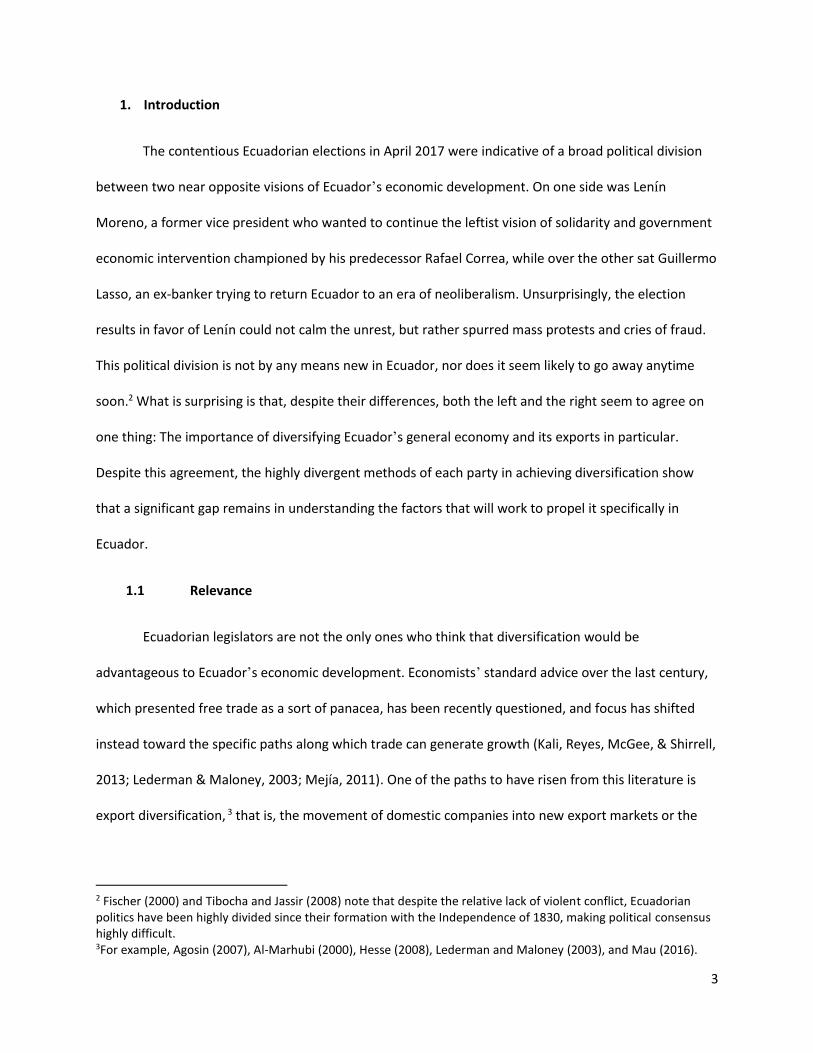

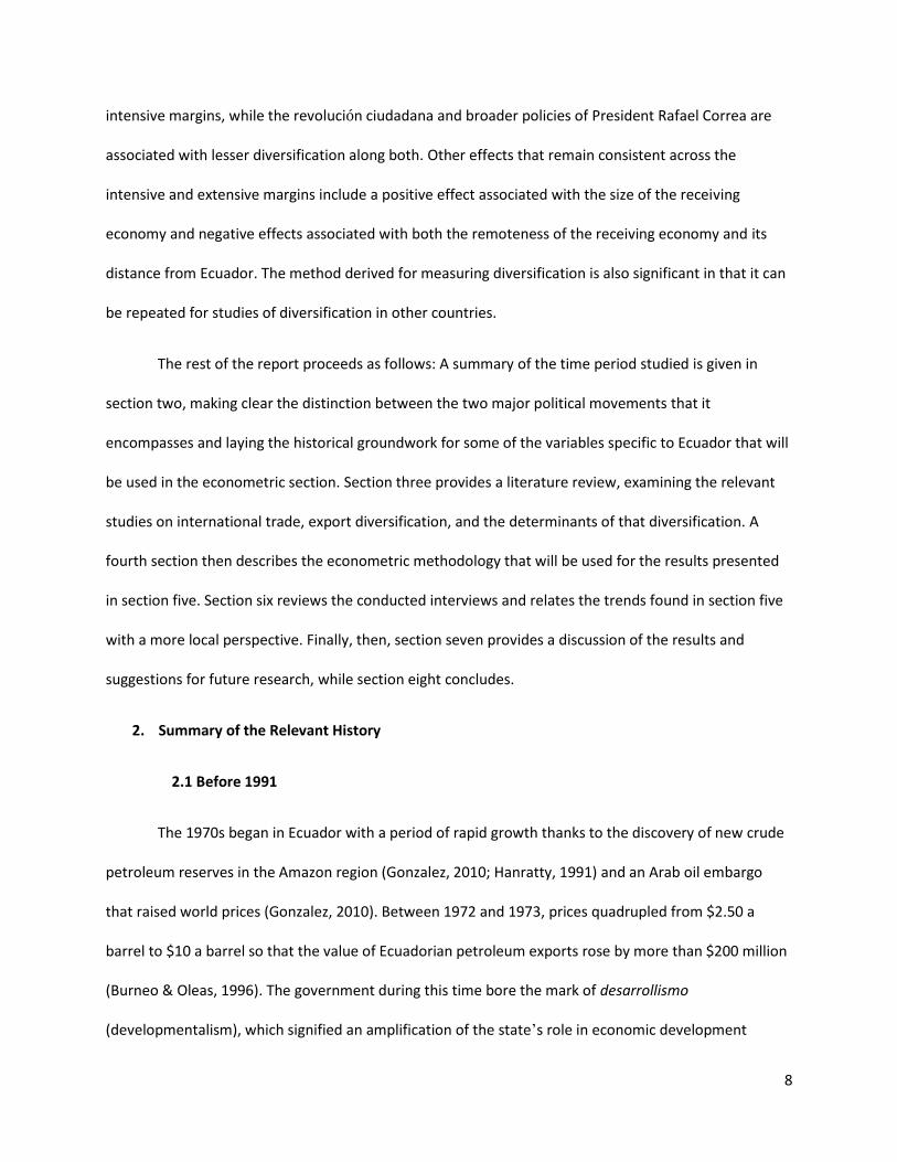


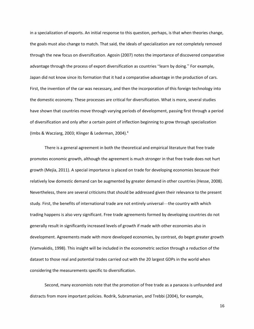


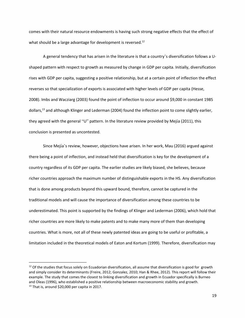
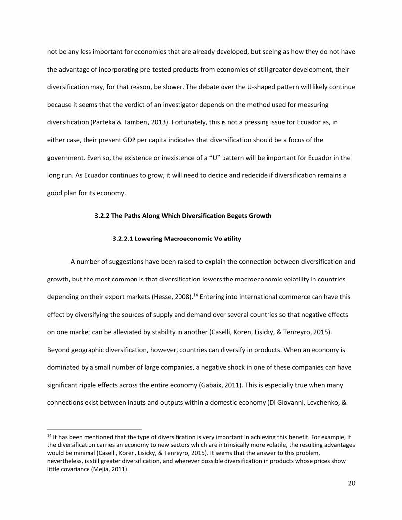
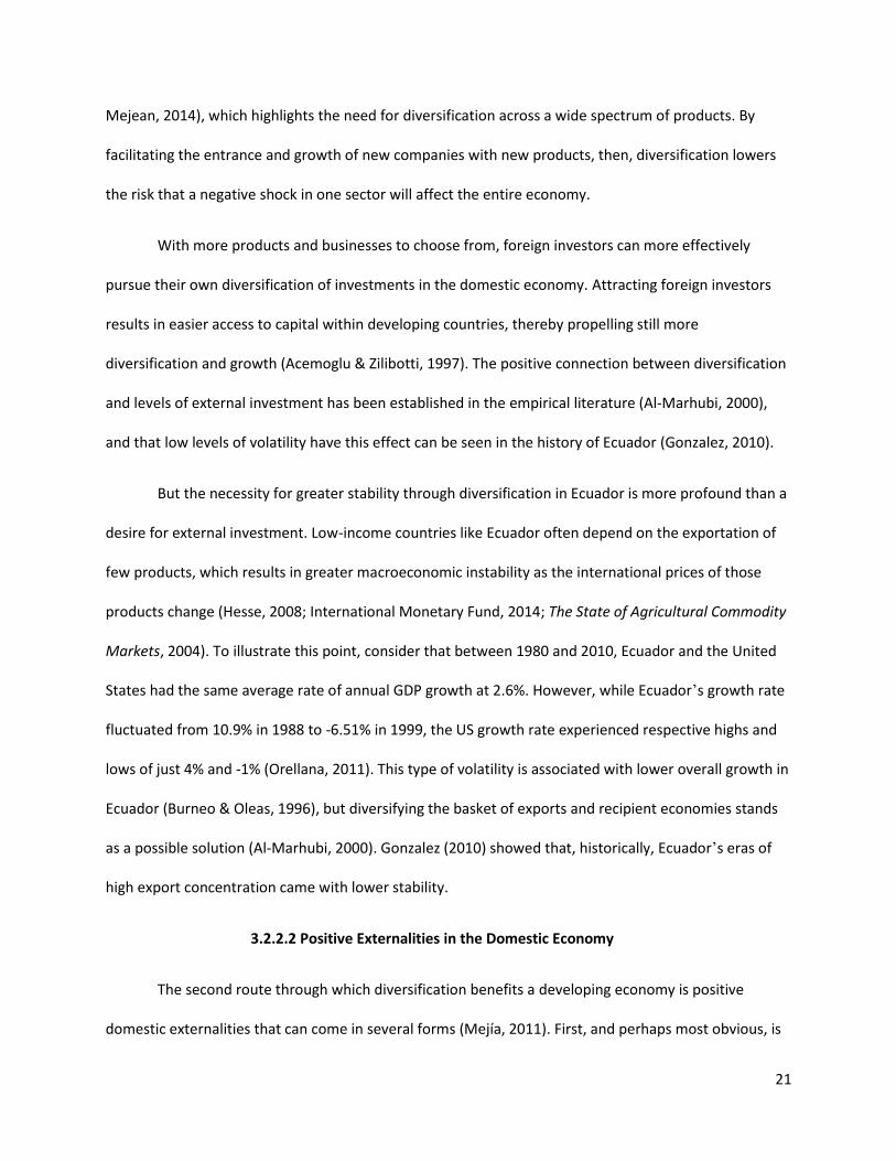

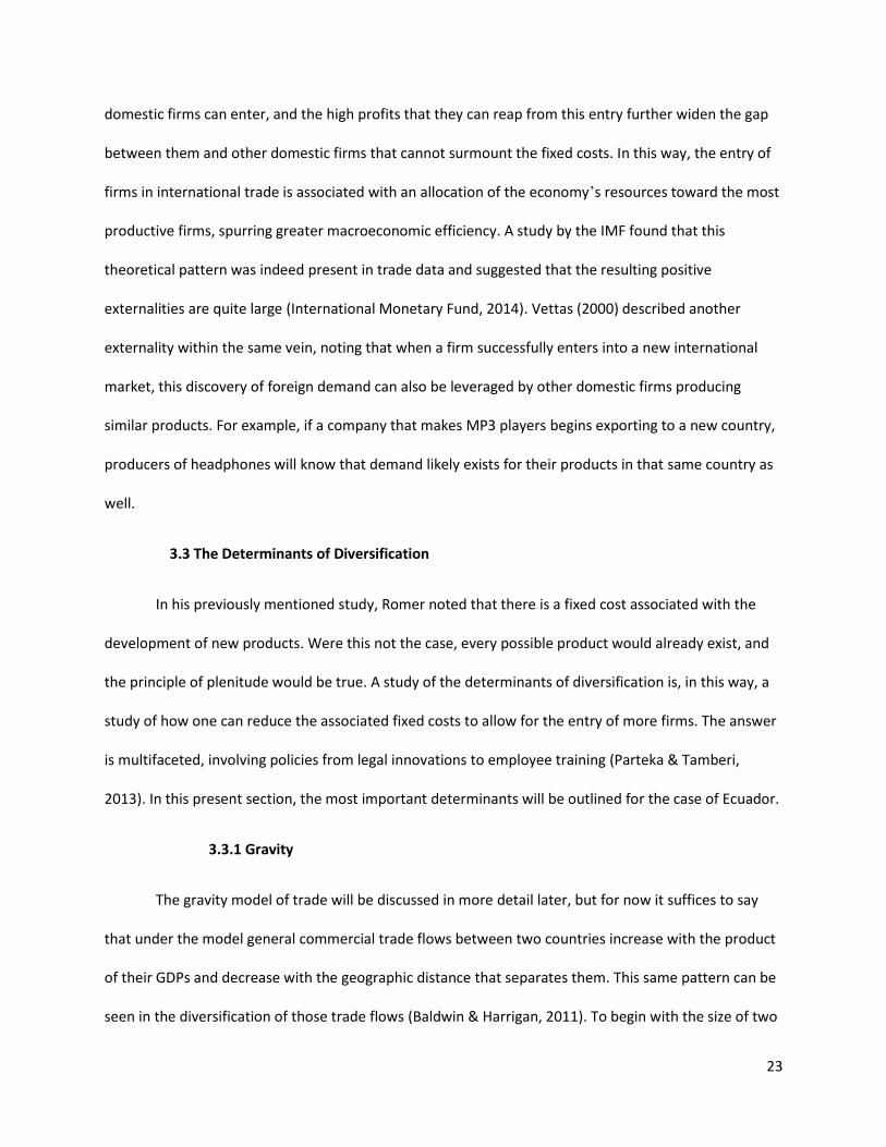
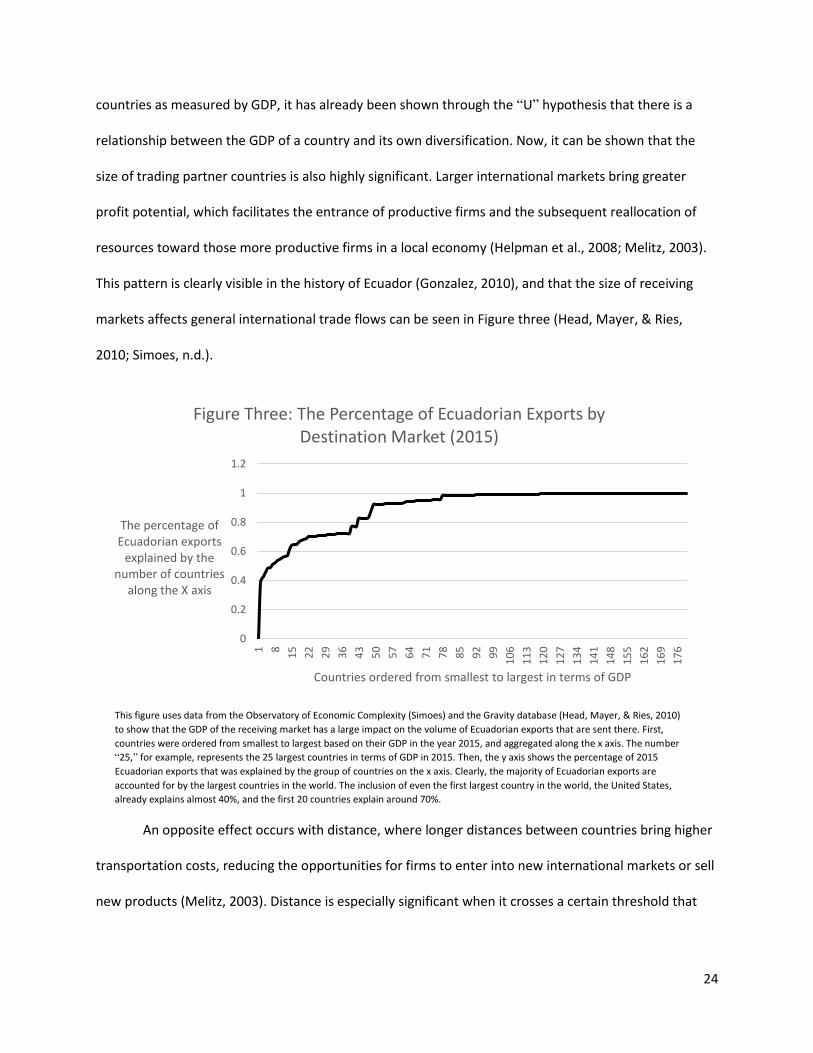


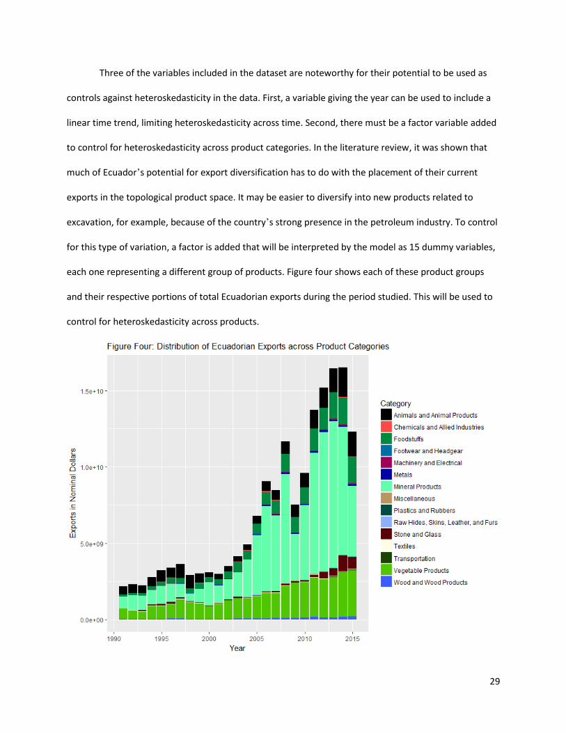
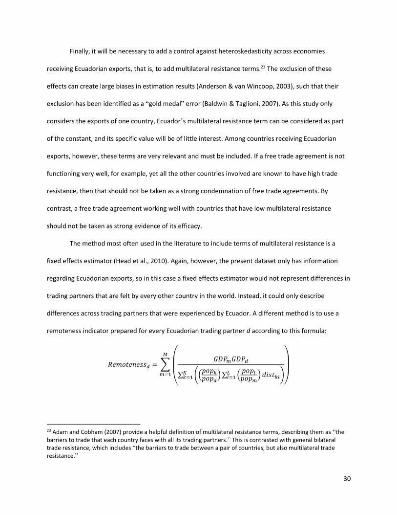
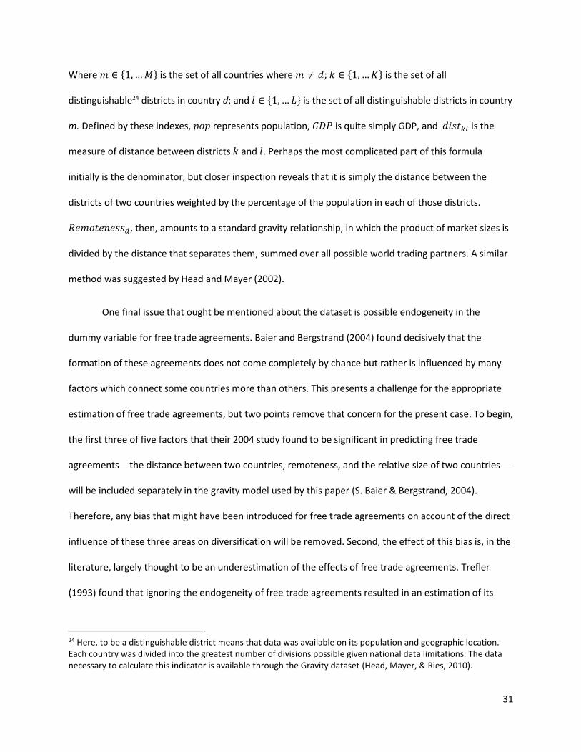


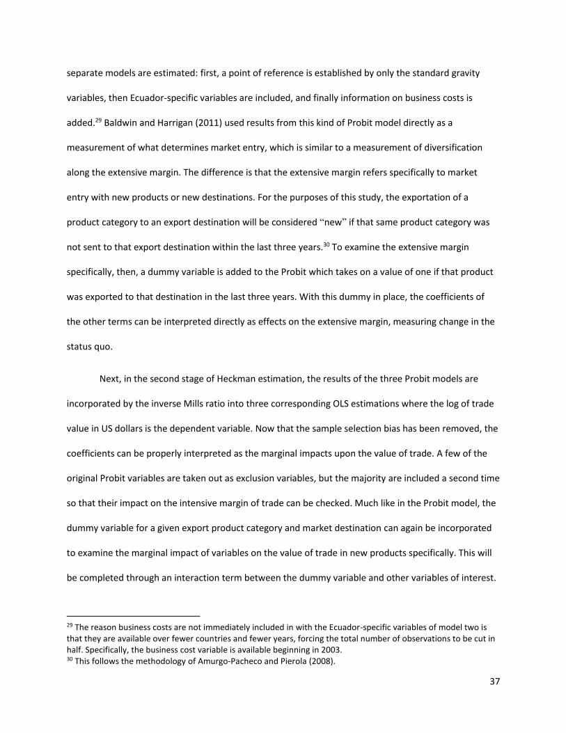
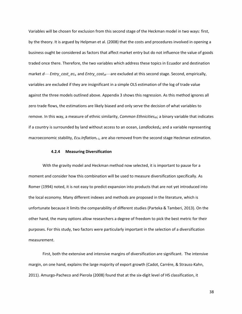


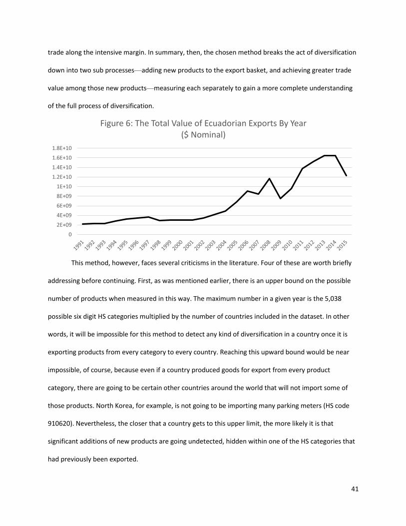

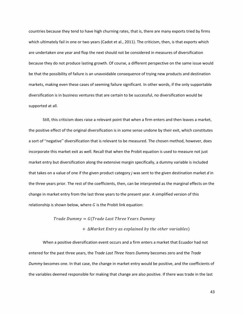
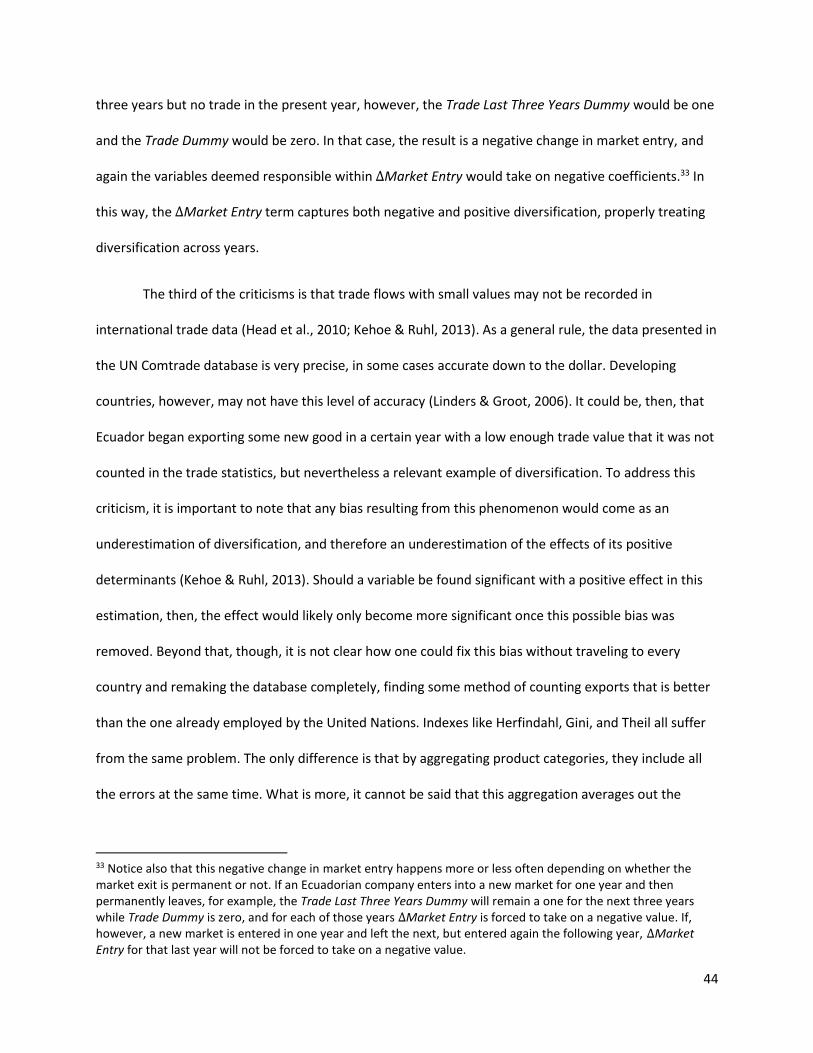


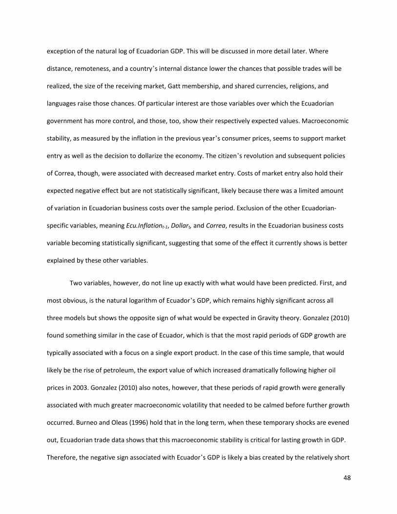
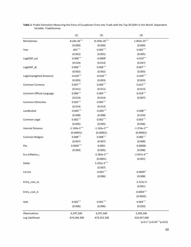
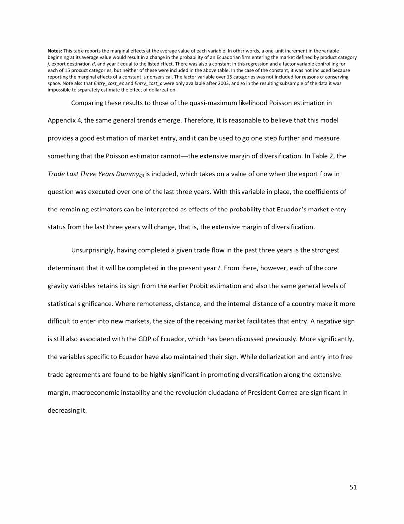
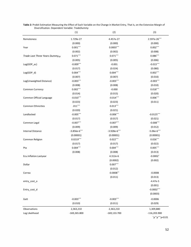
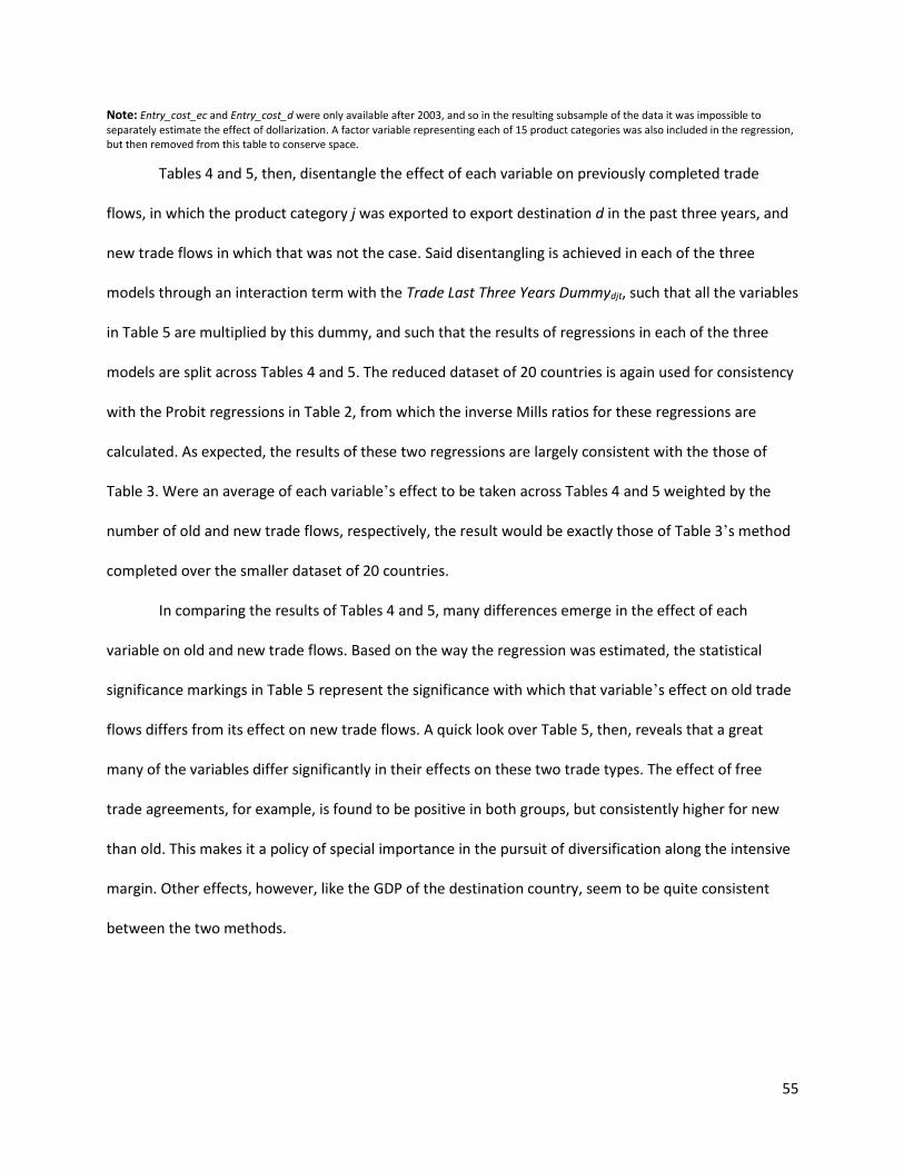
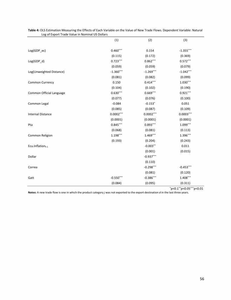


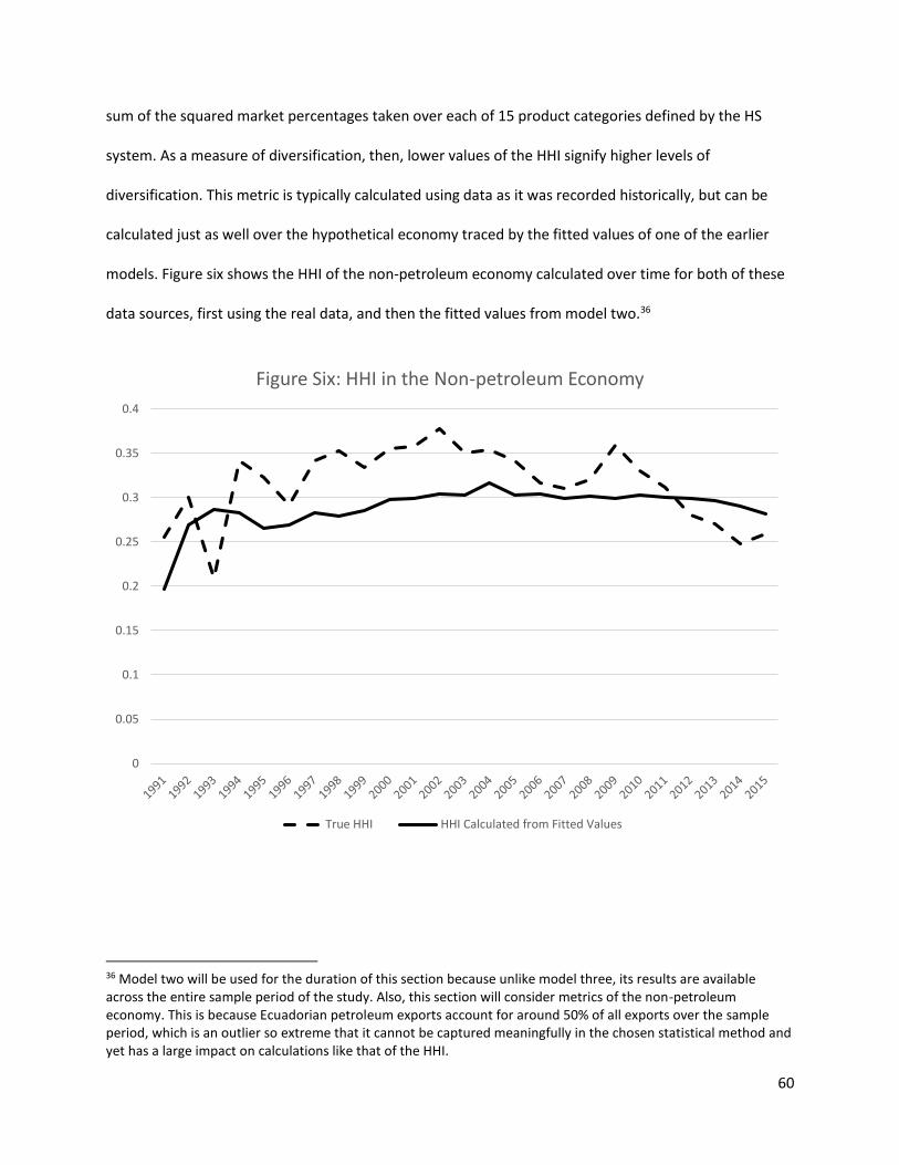


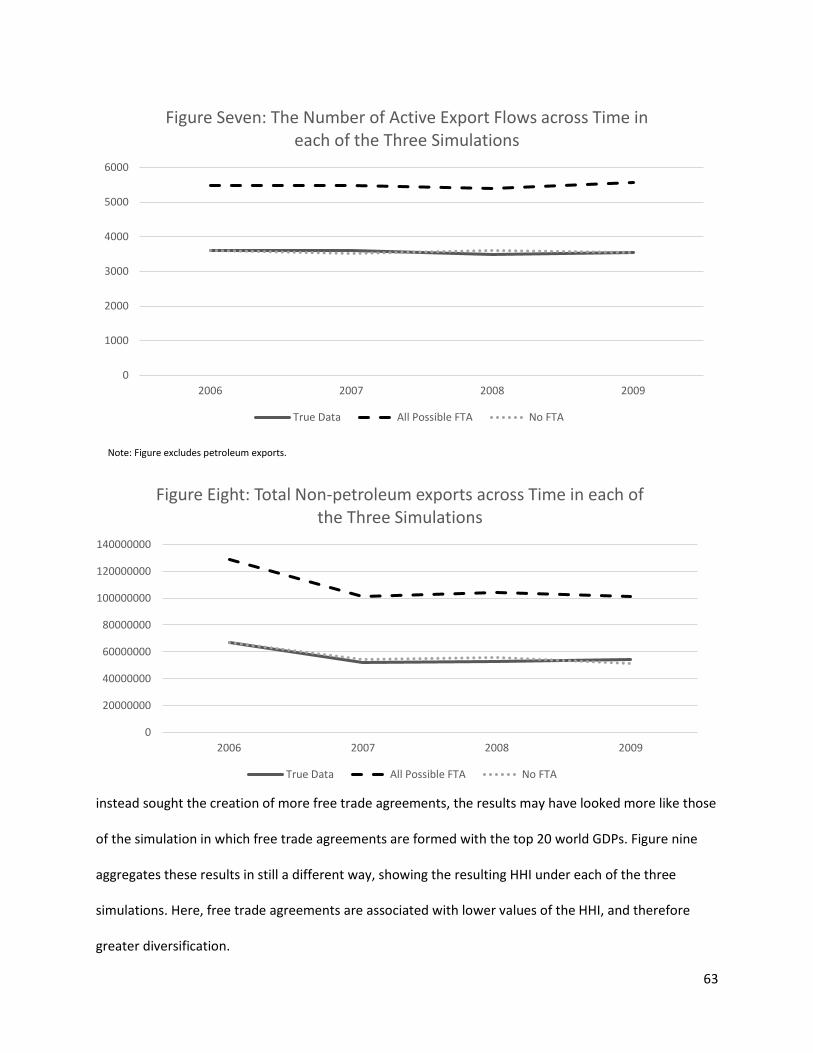
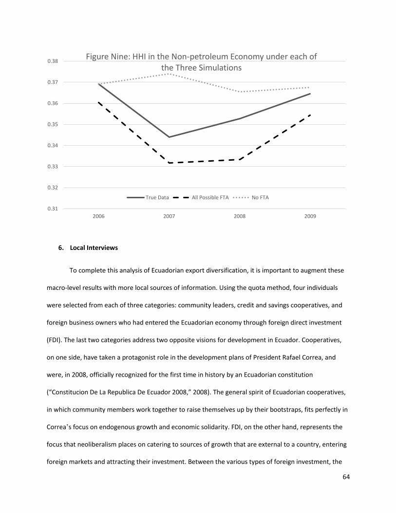


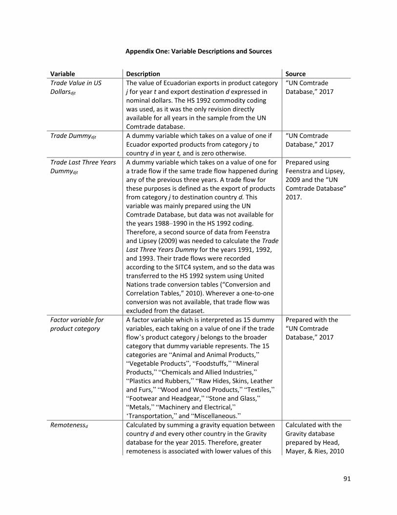
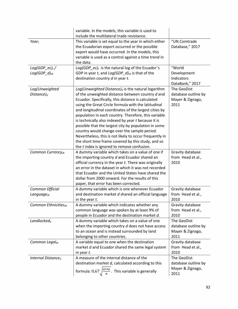

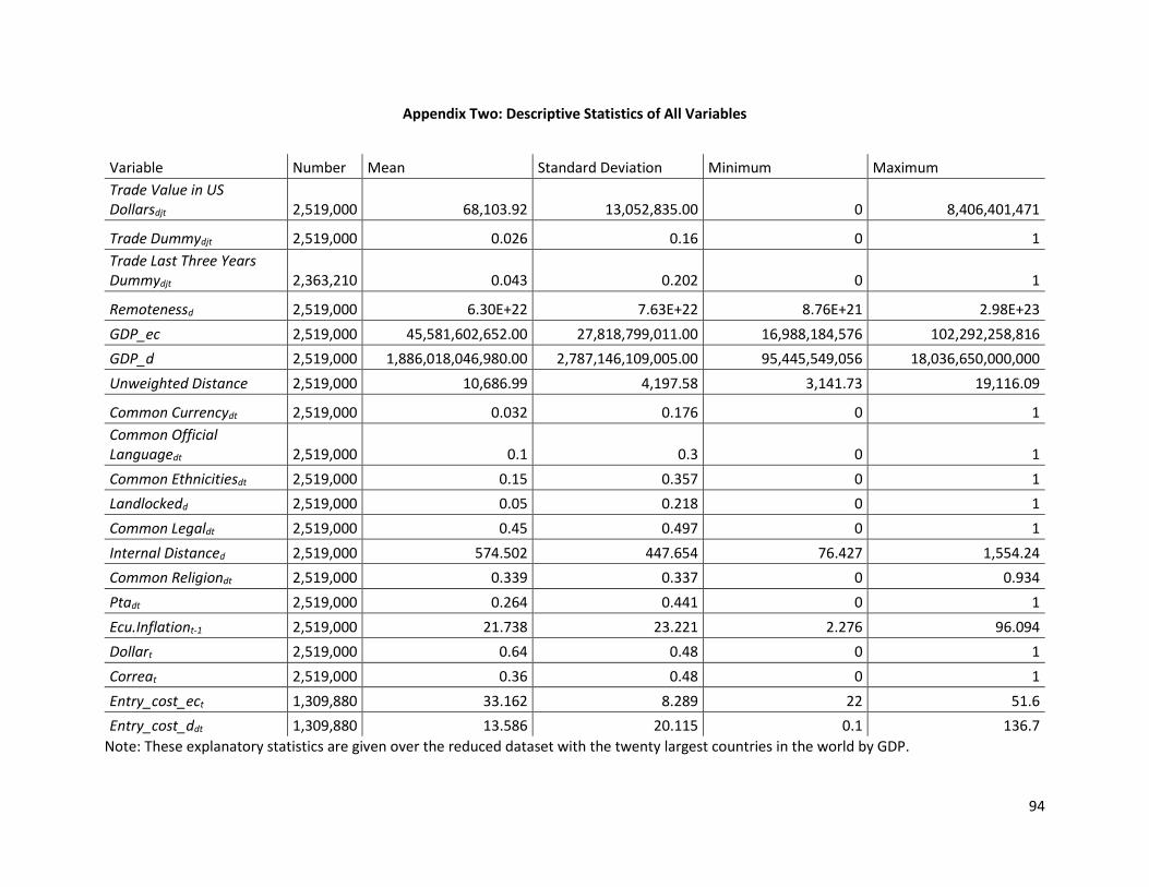
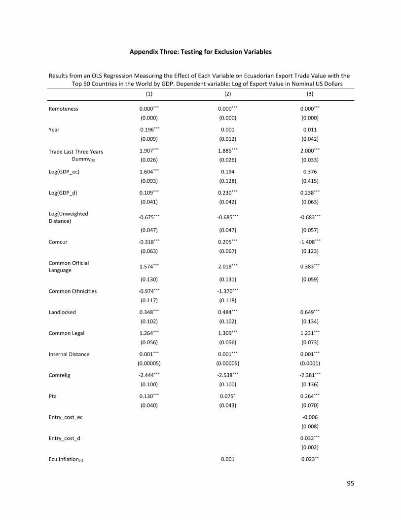
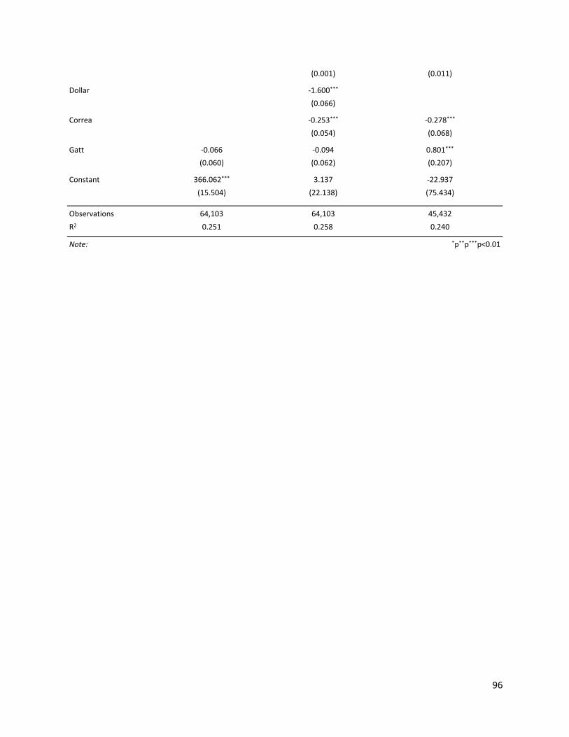

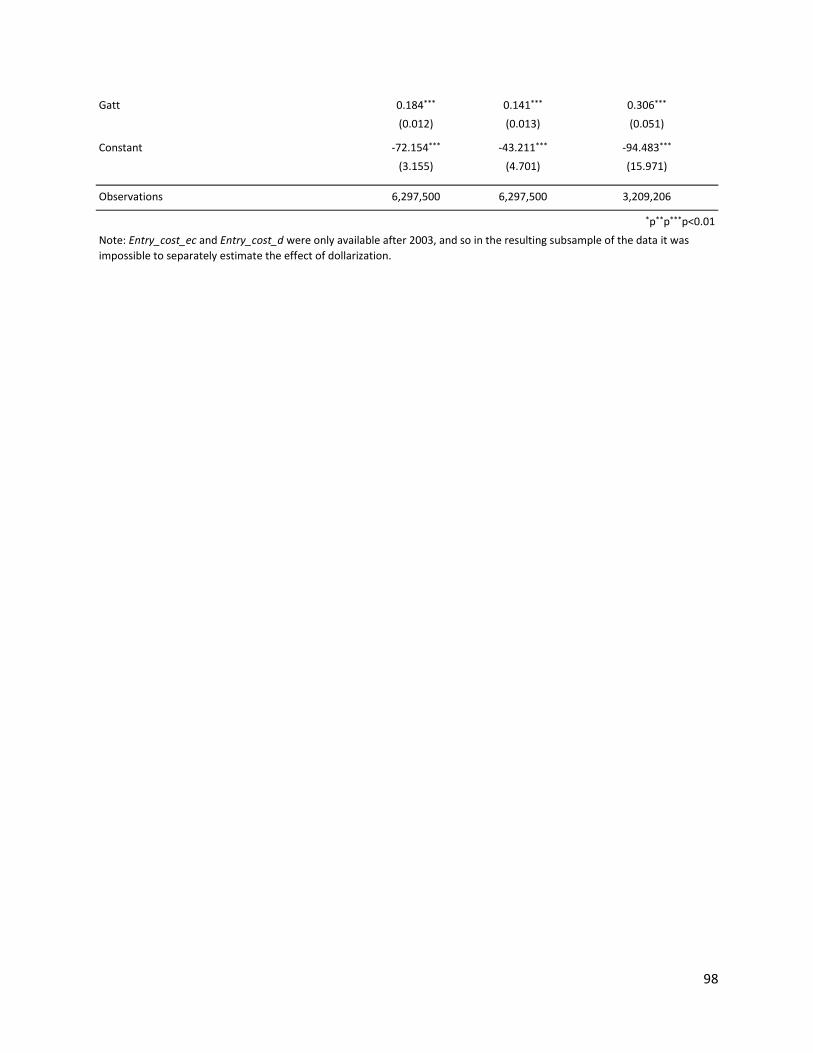


![Determinants of Agricultural Diversification in a Hotspot Area: … · 2018-05-16 · rural food insecurity and poverty in developing countries [2]. However, ... to estimate the determinants](https://static.documents.pub/doc/80x56/5e5347c230985962c3168b78/determinants-of-agricultural-diversification-in-a-hotspot-area-2018-05-16-rural.jpg)


