Determinants of Environmental and
Economic Performance of Firms: An
Empirical Analysis of the European Paper
Industry∗
Théophile Azomahoua, Phu Nguyen Vana ], and Marcus Wagnerb
a Bureau dÉconomie Théorique et Appliquée (BETA-Theme), Université Louis Pasteur
61 avenue de la Forêt Noire, F-67085 Strasbourg, France
b Centre for Environmental Strategy, University of Surrey
Guildford Surrey; GU2 7XH; United Kingdom
and
Center for Sustainability Management, University of Lüneburg
Scharnhorststr. 1, 21337 Lüneburg, Germany
∗Thanks to Jalal El Ouardighi, François Laisney, Anne Rozan, Marc Willinger and the
participants to the BETA-Theme seminar and Econometrics seminar at BETA, November
2001. We also acknowledge the participants to the International Summer School on Eco-
nomics, Innovation, Technological Progress, and Environmental Policy, Seeon (Bavaria),
8-12 September 2001. We retain responsibility for our errors.]Corresponding author: tel.: 33 (0)3 90 24 21 00; fax: 33 (0)3 90 24 20 71; e-mail:
[email protected] (Phu Nguyen Van)
1
Abstract
This paper examines the relationship between the environmental and
economic performance of Þrms in the European paper manufacturing indus-
try. Based on panel data, it Þrst investigates the relationship separately,
with the analysis based on four hypotheses formulated with regard to coun-
try inßuence, process inßuence and Þrm size inßuence on environmental and
economic performance. Hypotheses are tested using pooled regression and
a panel regression framework with random Þrm and temporal effects. The
main results of this analysis based on separated regressions are that (i) only
for a direct comparison between the UK and Germany, country effects are
found to be consistent with the hypotheses, i.e. German Þrms have better
environmental, but worse economic performance than UK Þrms, (ii) there
is a signiÞcant sub-sector effect on environmental performance only, (iii)
effectively no signiÞcant Þrm size effect can be detected. Subsequent to
analysing the relationship separately, the paper estimates the determinants
of the relationship between environmental and economic performance using
three simultaneous equations systems. It was found that for the system
with return on sales as economic performance variable, and an environmen-
tal performance index as environmental performance variable, a signiÞcant
and positive regression coefficient was estimated for the asset-turnover ratio,
as well as signiÞcant and negative coefficients for the dummy variables repre-
senting the industrial and mixed sub-sector. For the system with return on
capital employed and the environmental index, signiÞcant and positive coef-
Þcients were found for the latter, both linear and squared. This last Þnding
Þts better with traditionalist reasoning about the relationship between
environmental and economic performance, which predicts the relationship
to be uniformly negative.
Key words: Economic performance; Environmental performance; Paper
industry; Simultaneous equations system; Three-error-components model
JEL classification: C23; C30; L73; Q25
2
1 Introduction
The relationship between environmental and economic performance (i.e.
short-term proÞtability and longer-term competitiveness) of Þrms is an im-
portant issue for environmental policy making. In the current discussion
about this relationship, it is often argued that there is a conßict between
competitiveness of Þrms and their environmental performance (Walley and
Whitehead, 1994). For example, at the level of a speciÞc industry, the share
of environmental costs in total manufacturing costs might be considerably
higher than average (Luken et al., 1996). Particularly, this might be the case
for industries upstream in the production chain (such as primary resource
extraction or primary manufacturing), which have been shown to give rise
to environmental impacts disproportionate to the value added associated
with their production activities (Clift, 1998). It has therefore often been
argued that Þrms in such industries with higher environmental compliance
costs face a competitive disadvantage. Given that in the past, Þrms have
focused on end-of-pipe technologies as the major approach towards pollu-
tion control and environmental performance improvements in general, in the
traditionalist view, environmental investments were often seen as an extra
cost (Cohen et al., 1995).
Only recently, the notion emerged that improved environmental perfor-
mance is a potential source for competitive advantage as it can lead to more
efficient processes, improvements in productivity, lower costs of compliance
and new market opportunities (Porter, 1991, Porter and van der Linde, 1995,
and Schmidheiny, 1992), although this often refers to other aspects of en-
vironmental performance than those addressed and measured traditionally
(Wehrmeyer and Tyteca, 1998). Two major reasons to underpin this ar-
gument exist. Firstly, companies facing higher costs for polluting activities
have an incentive to research new technologies and production approaches
that can ultimately reduce the costs of compliance. But innovations also
result in lower production costs, e.g. lower input costs due to enhanced re-
source productivity (Porter and Esty, 1998). Secondly, companies can gain
Þrst mover advantages from selling their new solutions and innovations
to other Þrms (Porter and Esty, 1998). In a dynamic, longer-term perspec-
3
tive, the ability to innovate and to develop new technologies and production
approaches is likely a more important determinant of competitiveness than
traditional factors of competitive advantage, e.g. low-cost production, or
generally comparative cost advantages of a country (Porter and van der
Linde, 1995). This position can be termed the revisionist view.
So far, the relationships between environmental and economic perfor-
mance and its determinants have rarely been analysed in practice, partly
due to data constraints, partly due to a far-from-well-developed theoretical
framework. This paper attempts to discuss a number of important deter-
minants for the above relationship in order to develop hypotheses on their
expected inßuence. These determinants are initially though to be the coun-
try location of a Þrm, the industrial sub-sector it operates in, and the Þrm
size. For example, country-level regulation and innovation initiatives are
considered to have an inßuence on the relationship between environmental
and economic performance. Also, technological progress in industrial sectors
and sub-sectors is considered an important determinant that simultaneously
inßuences the environmental and economic performance of a Þrm, as is the
Þrms size. This obviously raises the question whether the theoretical propo-
sitions made with regard to key determinants of the relationship between
environmental and economic performance can be supported by empirical
evidence.
This paper therefore empirically analyses the inßuence of the aforemen-
tioned determinants on the environmental and economic performance of
Þrms in the European Union in a deÞned industrial sector. For this pur-
pose, data has been collected from corporate environmental reports and
emission inventories for the paper manufacturing industry in the Nether-
lands, Italy, Germany and the UK during the EU-funded project Measur-
ing Environmental Performance of Industry (MEPI).1 In parallel, Þnancial
1The project has been funded under the 4th Framework Programme (Environment
and Climate) of DGXII of the European Commission. Further information on MEPI
can be found at http://www.environmental-performance.org. MEPI was coordinated by
the Science Policy Research Unit SPRU, University of Sussex, UK. The research has
also been conducted by the Centre Entreprise-Société-Environnement CEE, Université
Catholique de Louvain, Belgium; the Institute for Environmental Studies, Vrije Univesiteit
Amsterdam, Netherlands, the Department of Economics and Production, Politecnico di
4
information for the same set of Þrms, for which environmental performance
data has been collected, has been extracted from Þnancial databases in a
comparable format for an number of accounting-based Þnancial indicators.
Based on this data set for a well-deÞned industrial sector (the paper man-
ufacturing industry), the paper analyses what factors determine to which
degree the environmental and economic performance of Þrms, as well as the
relationship between the latter two. Results of this research will inform en-
vironmental policy making in more detail about the factors which should
best be inßuenced in order to achieve a high effectiveness and efficiency of
policy measures. At the same time results also provide an indication about
the potential homogeneity or heterogeneity of determinants. This latter
point seems to be speciÞcally relevant for environmental policy, since it can
provide an indication about the degree to which policy measures need to be
differentiated depending on the country, sub-sector or Þrm population under
consideration.
Our empirical analysis involves an estimation procedure based on: (i)
a three-error-components panel data model for estimating separately the
determinants of economic performance and environmental performance; (ii)
a simultaneous equations system to account for the structural relationship
characterizing the joint determination of economic performance and environ-
mental performance. The main results emerging from separated regressions
are that (i) only for a direct comparison between the UK and Germany, coun-
try effects are found to be consistent with the hypotheses, i.e. German Þrms
have better environmental, but worse economic performance than UK Þrms,
(ii) there is a signiÞcant sub-sector effect on environmental performance only,
(iii) effectively no signiÞcant Þrm size effect can be detected. Subsequent
to analysing the relationship separately, the paper uses three simultaneous
equations systems. It was found that for the system with return on sales
as economic performance variable, and an environmental performance index
as environmental performance variable, a signiÞcant and positive regression
coefficient was estimated for the asset-turnover ratio, as well as signiÞcant
Milano, Italy; the Institut für Ökologische Wirtschaftsforschung IÖW, Austria; the
Institute for Prospective Technological Studies IPTS, Sevilla, Spain, and the Centre for
Environmental Strategy CES, University of Surrey, UK.
5
and negative coefficients for the dummy variables representing the industrial
and mixed sub-sector. For the system with return on capital employed and
the environmental index, signiÞcant and positive coefficients were found for
the latter, both linear and squared.
The paper is organised as follows: literature overview and theoretical
concepts motivating our own empirical approach are discussed in Section
2; the data collection methodology and sample description are presented in
Section 3; the econometric models used are described in Section 4; estimation
results are reported in Section 5. Section 6 concludes the study.
2 Overview and theoretical concepts
Based on these two contrasting positions described in the previous section,
two speciÞcations of the phenomenological relationship between the two con-
cepts of environmental performance (measured e.g. in terms of resource con-
sumption and emission levels) and economic performance (measured e.g. in
terms of stock market performance or Þnancial ratios) can be proposed. A
Þrst possible speciÞcation would be that the relationship between the two is
uniformly negative. This reßects the traditionalist view presented above
and is theoretically rooted in standard microeconomic theory, since pollu-
tion abatement measures in this theory are predicted to increase production
costs and are assumed to have increasing marginal costs (e.g. pollution
abatement and environmental performance improvements are assumed to
have decreasing marginal beneÞts and increasing marginal costs). This situ-
ation is depicted in Figure 1a below , where high environmental performance
(e.g., low normalised emissions and inputs) correspond to low economic per-
formance (i.e. low normalised proÞtability or market performance) and vice
versa.2 Generally, economic performance would be required, under the cir-
cumstances of Figure 1a, to be monotonously decreasing with increasing
environmental performance, i.e. the Þrst derivative (of economic perfor-
2 In the Þgures, environmental performance can be either an aggregate index of emis-
sions and inputs, or an environmental rating and economic performance can be an indi-
vidual Þnancial ratio (return on sales or assets, value added per employee) or an aggregate
index of Þnancial or economic performance of a Þrm.
6
mance differentiated to environmental performance) is always negative. In
addition to that, the second derivative is required to be negative, repre-
senting an increasing negative marginal impact of increasing environmental
performance on economic performance.
Figure 1 about here
However, the relationship between environmental and economic perfor-
mance of Þrms does not have to be unidirectional, but can be changing
from positive to negative or vice versa. A second possible speciÞcation for
the relationship would therefore be an inversely U-shaped curve across the
environmental performance spectrum. Such a speciÞcation would also be
theoretically supported by standard microeconomic theory, but would also
be taking into account the innovation aspects brought forward in the revi-
sionist perspective. Based on this the relationship between environmental
and economic performance can be represented through a bell-shaped (i.e.
inversely U-shaped) curve. It is upward-sloping for Þrms with environmen-
tal performance below the optimum (which is the point where economic
performance is maximised). This means that the beneÞts reaped from in-
creased environmental performance increase continuously for low levels of
environmental performance. This curve holds up to a certain point around
or slightly above average environmental performance.3 Beyond this point,
the relationship is likely represented by a downward sloping curve (which
in a Þrst approximation is considered to be fairly linear). Taken together,
the shape of the relationship over the whole spectrum of environmental
performance encountered would be an inversely U-shaped curve with an
optimum point (i.e. a level of environmental performance, where the ben-
eÞts for economic performance net the costs for achieving this level are
maximised over the whole spectrum). Schaltegger and Figge (2000) have
expanded on this, pointing out that the discussed relationship in general is
neither positive, nor negative. They consider the relation to follow a gener-
3 It is an interesting question, where exactly the optimum (i.e. economically efficient)
level of environmental performance lies, since this would shed considerable light on the
degree to which pollution prevention pays. However, this is beyond the scope of this
exposition of possible speciÞcations.
7
alised bell-shaped/inversely U-shaped curve with a monotonously decreasing
Þrst derivative and a negative second derivative (i.e. an increasing negative
marginal impact on economic performance from increasing environmental
performance). The part of the curve which lies to the left of its maximum
(i.e. the optimum level of environmental performance which corresponds to
maximum economic performance) is characterised by a positive Þrst deriva-
tive and a negative second derivative. The part of the curve which lies to
the right of its maximum is characterised by a negative Þrst derivative and
a negative second derivative. This speciÞcation of the relationship (a syn-
thesis of the traditionalist and revisionist views) is depicted in Figure
1b.4
These considerations allow to conclude that economic theories (particu-
larly standard microeconomic theory and the theoretical reasoning behind
the Porter hypothesis) propose the generalised relationship between environ-
mental and economic performance to be a inversely U-shaped (i.e. concave)
relationship, as depicted in Figure 1b. Following the argument above by
Schaltegger and Synnestvedt (1999) a generalised bell-shaped/inversely U-
shaped curve would represent the best possible case for the relationship
between environmental and economic performance, since it allows for the ex-
istence of win-win situations with proÞtable (in the short-term) environmen-
tal performance improvement activities. On the other hand, a monotonously
falling curve would represent the traditionalist view. This would corre-
spond to a situation where at the phenomenological level environmental
performance improvements can only increase costs and reduce proÞts. Un-
der such conditions, the optimal level of environmental performance would
be that prescribed by environmental regulations, i.e. compliance.
However, the interaction of environmental and economic performance
(being represented at a very aggregated level by the phenomenological rela-
tionship between the two concepts as discussed so far) is in a causality per-
spective (i.e. regarding the causes of the relationship) most likely indirect,
through factors inßuencing either environmental or economic performance,
or both and should thus be perceived as the outcome of a complex process
4The environmental performance and the economic performance axis are deÞned as in
Footnote 2.
8
of interaction and inßuence. In this process, the inßuence factors have a
causal relationship to environmental and/or economic performance. Prior
to generating hypotheses with regard to individual factors, the interaction
between environmental and economic performance needs to be discussed in
more detail. In order to do so, a more general model linking 1) inßuence
factors, 2) environmental performance, and 3) economic performance needs
to be developed. Therefore, in Figure 2, a model is shown for the inter-
action between inßuence factors, environmental performance and economic
performance. In this model, the phenomenological relationship is related
to the inßuence of moderating factors discussed above. The phenomeno-
logical relationship between environmental and economic performance is
represented at the top level of the model. This is, what is observable (e.g.
by way of a scatterplot of individual environmental performance indicators
against Þnancial indicators).
The model in Figure 2 shows the factors considered most important
which cause a certain level of environmental and economic performance.
In the most general form it should be assumed that each of these factors
have a simultaneous inßuence on environmental and economic performance.
However, it may well be possible that each factor can be considered to have
a predominant inßuence on either environmental or economic performance,
since the key factors inßuencing most directly and strongly environmental
performance are possibly relatively distinct to these that inßuence economic
performance.
Figure 2 about here
Next to the different inßuences (in terms of directness and strength) the
factors at the bottom of Figure 2 have on environmental and economic per-
formance, there are two more noteworthy aspects. Firstly, the inßuencing
factors also interact amongst each other. For example, Þrm size can have
an inßuence on corporate environmental strategies/management: it is often
argued that small Þrms are laggards who have a relatively reactive stance
towards environmental management (Bradford, 2000). As well country lo-
cation (via environmental regulation) can have an inßuence on the processes
operated: for example in Germany, the Kraft pulping process is indirectly
9
prohibited through very stringent emission limits for pulp manufacturers,
whereas in other countries, limits are not as strict and thus operation of the
Kraft process is possible (Ganzleben, 1998, p. 24). If the inßuences and
interaction between any two inßuencing factors are very direct and/or very
strong, this needs to be taken into account. They can only be neglected,
if the interaction between any two factors are very weak and very indirect
compared with the inßuences each moderating factor has on environmental
and/or economic performance.
Secondly, a number of additional factors need to be considered which
have an inßuence exclusively on economic performance. Amongst these are
investors and their expectations of return, changing market conditions with
regard to demand, supply and prices, the cyclic nature and/or the average
capital intensity of the industries under consideration. Given these poten-
tial inßuences mainly on economic performance, the model described above
might have to be expanded as depicted in Figure 3.
Figure 3 about here
As can be seen in the model in Figure 3, the additional factors which
mainly have an inßuence on economic performance can potentially also in-
ßuence the set of inßuencing factors introduced in Figure 2 (which are con-
sidered to inßuence environmental and economic performance), hence, this
interaction needs to be taken into account as well.
Based on the two models developed above, several hypotheses can be
derived with regard to the most important inßuence factors inßuencing the
relationship (environmental management, industry structure, processes op-
erated, Þrm size and inßuence of regulation). In the following, the relevant
inßuencing factors considered relevant in the Þrst model (Figure 2) shall
therefore be discussed in more detail in order to justify their theoretical rel-
evance, particularly that they are likely to be the most important factors
inßuencing environmental performance. In the following, hypotheses are
therefore formulated regarding the inßuence of these factors on environmen-
tal and economic performance, respectively. This will concern the following
factors necessary to explain (at least part of) the full variance encountered
in the data set with regard to the relationship between environmental and
10
economic performance: (i) country location (which proxies for level and
efficiency of regulation in an industry), (ii) processes operated (which are
proxied at least partly by individual Þrm effects), and (iii) Þrm size.5
The inßuence of the industry market structure/sector membership can-
not be assessed with the data set at hand, since this only comprises of
Þrms in the paper manufacturing sector in the EU. The additional factors
in Figure 3 will also not be considered, since they are either industry- or
country-related. In the former case they are assumed to be constant in their
inßuence (since only the paper manufacturing sector is considered). In the
latter case, they are captured in the country dummy variables included in
the regressions.
Country location
Country-level inßuences on the relationship between environmental and
economic performance have so far often been excluded from the analysis,
partly due to the dominance of US-based studies (focusing on only one
country). To better understand the relationship between environmental
and economic performance, a Europe-based study therefore seems neces-
sary and timely. Country location proxies jointly for a number of inßuences.
This can e.g. be the level of stringency of environmental regulations, the
type of instruments used to implement these (e.g. economic instruments, or
command-and-control legislation) which has an inßuence on the efficiency of
environmental regulation in different countries, or the level of general busi-
ness taxes in the country. The joint inßuence of these factors is captured in
the country location. It is very well possible that the relationship between
environmental and economic performance at the Þrm level is affected by dif-
fering country inßuences, if Þrms are not all located within one country. In
such a case, country inßuence needs to be examined closely prior to drawing
5The inßuence of environmental management systems was not included in the analyses
reported here, since there is evidence for the data set used, that it is not a good measure,
since Þrms have no signiÞcantly different environmental performance, regardless of whether
they have a certiÞed Environmental Management System (EMS) or not (Wagner et al.,
2001). In addition to that, for 1995, none of the Þrms in the data set had a certiÞed
EMS. Also, it is theoretically possible that Þrms without a certiÞed EMS carry out the
same environmental management activities as those which are certiÞed. Nevertheless,
information on EMS has been included in Table 2 below.
11
conclusions for a complete set of Þrms from different countries.
The most important factor in the context of this research is likely the
regulatory regime in a country in general and for speciÞc industries, i.e. the
strictness of an approach to environmental legislation and regulation.6
If it is accepted that country inßuences on the relationship between en-
vironmental and economic performance result from the fact that in different
countries the stringency of, as well as the approach to (and thus the effi-
ciency of) environmental (and to a lesser degree other) regulation may differ,
then under the assumption that Þrms are compliance-oriented (and not over-
compliant) it can be expected that the level of environmental performance
(i.e. the emission levels) of a Þrm is (linear) proportional to the stringency
of environmental regulation (which can be measured as, e.g., the average
level of emission standards in a country).7 The reason for this relationship
between stringency of regulation and environmental performance is that ini-
tially it only pays for Þrms to pursue emission reductions until they meet
the emission standards for their industry, since only such reductions yield an
economic beneÞt for Þrms in terms of minimizing their compliance costs by
avoiding Þnes. In a compliance-oriented situation, the environmental per-
formance of a Þrm (measured in terms of its emissions) can be considered as
a revealed regulatory stringency (as opposed to a stated regulatory strin-
gency as expressed by emissions standards). A situation of over-compliance
is unlikely, since over-compliance would only be rational for Þrms if it can be
achieved through cost-effective pollution abatement measures. Most cost-
effective measures have however amortisation periods of more than 2 years
so that annualised returns can usually not compete with other investment
6A third important aspect is the degree of certainty, in a country, regarding the future
development of environmental regulation. This aspect is however very difficult to capture
and is therefore excluded in this paper.7The same situation applies equally to sectoral differences in regulation. For example,
Henriques and Sadorsky (1996) argue that costs of regulation differ across industries, and
that Þrms in more regulated industries are more likely to embed environmental issues into
their management strategies since the costs associated with non-compliance tend to be
signiÞcantly higher (p. 385). Nevertheless, differences with regard to regulation seem to
be much more pronounced between countries, since within one country usually one speciÞc
regulatory body and process produces environmental regulation for various industries.
12
options. In addition to that, over-compliance needs a Þrms careful consid-
eration since it could signal to regulators a scope for tighter environmen-
tal regulations without signiÞcantly affecting companies proÞtability and
competitiveness. Therefore over-compliance can be expected to be the ex-
ception, rather than the norm. Nevertheless, the effect of distortions from
over-compliance (resulting, for example from Þrms anticipation of future
tightening of regulations) needs to be taken into account and assessed prior
to assuming the above relationship between stringency and performance.
Next to the strictness/stringency of environmental regulation, it is also
necessary to consider the efficiency of regulation depending on the instru-
ments used. From the point of economic theory it is usually argued that
the use of economic instruments is more efficient than a command-and-
control approach. For example, some countries have generally a very strong
legal stance in their environmental regulation, whereas others lean more
towards economic instruments, such as taxes or subsidies, and yet others
tend to prefer voluntary or negotiated agreements. Germany, the UK and
the Netherlands would be respective examples. However, it is at times dif-
Þcult to distinguish such regimes clearly, since governments usually apply
a mix of economic, legal and voluntary or negotiation-based instruments
simultaneously. However, it has also to be taken into account, to what de-
gree regulations are designed and implemented efficiently and are enforced
properly.8
In Germany and the UK, the extent of corporate environmental protec-
tion has increased signiÞcantly over the last decade. The socio-political, reg-
ulatory and economic climates of the two countries show clearly differences,
which has meant that companies in each country have developed manage-
ment approaches and corporate environmental strategies that are speciÞc
to their national circumstance, with likely different inßuences on the envi-
ronmental and economic performance of Þrms. For instance, Gordon (1994)
acknowledges that, whilst awareness of broader political and social aspects
8This is a particularly important issue, since properly designed environmental regula-
tion in the Porter hypothesis is expected to produce organisational and technical innova-
tions which lead to production efficiency gains that can result in competitive advantages
compared to less stringent regulation (Porter and van der Linde, 1995).
13
in environmental policy is greater in Britain, the level of analysis and the
efficiency of environmental policy making is often greater in Germany. Peat-
tie and Ringer (1994) report strong enthusiasm for environmental manage-
ment amongst British companies, and suggest that in organisational terms,
they are not signiÞcantly lagging behind, but may increasingly do so due to
weak environmental legislation. James et al. (1997) Þnd that for speciÞc
socio-political dimensions, such as stringency of regulation, the character
of existing competitive strategies within Þrms, or the level and quality of
public concern for environmental issues, have led to distinct environmental
management types in both countries, with likely different inßuences on en-
vironmental and economic performance, and, ipso facto, the relationship of
the latter two.
Compared to Germany and the UK, in the Netherlands, two key trends
in Dutch policy inßuenced the situation with regards to European Eco-
Management and Auditing Scheme (EMAS). This is Þrstly the strong stance
for deregulation (also concerning environmental regulation) in the early as
well as the rising level of political and public environmental awareness in
the late 1980s (Wätzold et al., 2001). Within the Dutch National Envi-
ronmental Policy Plan in particular, this implied two speciÞc new strate-
gies. Firstly, this was the introduction of Environmental Management Sys-
tems (EMS) within industry target groups, and secondly, the negotiation of
agreements (so-called covenants) in which the target groups contributions
to the achievement of various environmental policy goals (e.g., greenhouse
gas emission reductions) were deÞned (Wätzold et al., 2001).9
Based on WEF et al. (2001), the stringency of regulation and the ori-
entation of regulation towards ßexible instruments (as a proxy for the effi-
ciency of environmental regulation) of the four countries (Germany, Italy,
the Netherlands and the United Kingdom) studied in this paper can be
classiÞed as in Table 1.
Table 1 about here9Regulatory relief was granted equally to EMS veriÞed under EMAS or certiÞed under
ISO 14001.
14
As stated above, with regard to level (i.e. strictness of regulation), effi-
ciency (determined by the approach to regulation) and future development
of environmental regulation, it can therefore be expected that the level of
environmental performance will be higher in countries and sectors with (i) a
higher stringency of environmental regulation (i.e. more stringent emission
standards), and (ii) a more efficient approach to regulation. In particular,
the reason for (ii) is that despite the limitations of the mechanisms proposed
by the Porter hypothesis, it is likely that incentive-based regulations using
economic instruments or voluntary reduce private and social abatement costs
as compared to command-and-control type regulation. Incentive-based reg-
ulations maintain incentives for Þrms in an industry to reduce emissions,
provide cost-effective allocation of resources and abatement technologies
and therefore at least reduce the negative impact of environmental regu-
lation on Þrm proÞtability and competitiveness. Therefore, the following
two hypotheses are proposed:
Hypothesis H1: In countries with more stringent regulation, Þrms are
expected to have signiÞcantly better environmental performance, as well
as signiÞcantly worse economic performance, than in countries with less
stringent environmental regulation.
Hypothesis H2: In countries, where regulations are more oriented to-
wards economic instruments, environmental, as well as economic perfor-
mance are expected to be more positive than in countries where regulation
is more oriented towards command-and-control type regulation. As a result
of this, the relationship between environmental and economic performance
is expected to be more positive.
Processes operated
Generally, the processes operated at a site are more a classiÞcation cri-
terion, rather than a inßuencing factor to be hypothesised about, since only
Þrms and sites with fairly comparable processes per se can be compared
with regard to the relationship between environmental and economic per-
formance. Processes operated are therefore operationalised in this research
by means of a broad classiÞcation scheme, in which newsprint, magazine-
grade and graphics Þne paper are represented by one category cultural
papers, and packaging corrugated and other boards by another category,
15
industrial papers. Also mixed and other categories were deÞned, re-
sulting in a classiÞcation based on four (broad) sub-sectors . One important
reason for introducing a mixed sub-sector is the fact that the actual unit
determining the product is not the site, but the individual paper machine.
Since one site usually runs more than one paper machine, it is often the case
that two different products are produced at that site. A sub-sector category
mixed accounts for this. Sub-sector dummy variables were introduced as
control variables since it is assumed that the economic performance of a
Þrm strongly depends on the sub-sector it operates in, and that also envi-
ronmental performance may be inßuenced by sub-sector membership. Given
this, signiÞcant sub-sector effects can be detected by including a sub-sector
dummy. Therefore, the following hypothesis shall be tested:
Hypothesis H3: The environmental and economic performance of Þrms in
one industrial sector is expected to vary signiÞcantly across its sub-sectors,
i.e. there are signiÞcant differences in economic performance, environmental
performance, and, ipso facto, the relationship between environmental and
economic performance is expected to differ signiÞcantly across the different
sub-sectors.
Firm size
It is often argued that Þrm size has an inßuence on corporate environ-
mental performance, as well as on its relationship with economic perfor-
mance. One reason for this is that Þrm size can be used to reßect Þrm visi-
bility, and, since larger Þrms tend to be more susceptible to public scrutiny,
they are more likely to be industry leaders with regard to environmental
performance (Henriques and Sadorsky, 1996). In addition to that, smaller
and medium-sized Þrms are considered to be in many ways laggards who
have a relatively reactive stance towards environmental management (Brad-
ford, 2000).10 Small and medium-sized Þrms (SMEs) are often found to be
unaware of their legal duties regarding waste disposal and frequently do not
consider their operations having a signiÞcant environmental impact. In ad-
10Usually, small Þrms are deÞned as those with less than 50 employees, whilst medium-
sized companies are considered to be those in the range of 50-250 employees (EIM, 1997, p.
329). Such a deÞnition however needs to account for potential distortions from transitory
growth and size class changes of Þrms (Wagner, 1995).
16
dition to that they tend to be unfamiliar with environmental management
systems and standards and respond strongest to regulation as a stimulus for
environmental improvement (Bradford, 2000, and Meffert and Kirchgeorg,
1998).
This experience from a research project looking at Environmental Aware-
ness in SMEs in Þve EU countries (Germany, Sweden, the Netherlands, Italy
and the UK) is also supported by a Swedish survey which found in 1998
that small Þrms with less than 50 employees in Sweden had no signiÞcant
ambition to become environmental leaders although attitude changes were
noted in medium-sized companies above 50 employees, mainly triggered by
the introduction of EMS, customer requirements and organizational change
(Heidenmark and Backman, 1999). Consistent with this empirical experi-
ence it is found that competitiveness is the highest priority for SMEs, whilst
avoidance of legal problems (under which environmental performance can
be subsumed to a large degree due to the fact that SMEs were found to be
mainly compliance- and regulation driven) are ranked very low (Bradford,
2000).
Implied by the above considerations is that, so far, SMEs themselves
mainly perceive the relationship between environmental and economic per-
formance to be negative or at least non-existence, since competitiveness (as
a basis for good economic performance) is not considered to be linked to
legal problems (such as breaches of environmental standards) or is thought
to be conßicting with the avoidance of legal problems.
Economic theory provides mainly four reasons for differences in Þrm
size and thus of different levels of market concentration (You, 1995, and
Moschandreas, 1994). These are:
the existence of U-shaped or L-shaped long-term average cost curves,
i.e. a minimum efficient scale of production (MES) exists (the production
theory justiÞcation);
the existence of transaction costs, resulting in a substitution of alloca-
tion mechanisms, i.e. Þrms as organizational structures instead of markets
(the transaction cost theory-based justiÞcation);
the existence of heterogeneous (monopolistic, incomplete) competi-
tion, i.e. markets with many sellers and differentiated products (justiÞcation
17
based on demand conditions in the market) which postulates niche markets
for small Þrms; and
the stochastic explanation often modeled as a Gibrat process following
the law of proportionate effect (justiÞcation based on the notion that changes
in concentration are the net effect of a large number of uncertain inßuences).
Basically these economic approaches to explain differences in Þrm size
allow the conclusion that small Þrms exist where this is not a competitive
disadvantage, e.g. where MES or transaction costs are low, or where the
market structure allows the existence of niche markets. As far as the re-
lationship between environmental and economic performance is considered,
this would imply that from the point of economic theory, no direct explana-
tion is provided as to why the relationship should be less positive for smaller
Þrms than for larger Þrms (although, as explained above, precisely this is
the self-perception of SMEs).11
Nevertheless (and possibly explaining empirical Þndings) it is possible
that for SMEs a less positive relationship exists if there are economies of
scale in environmental management systems and activities. This is well
possible, since environmental management is likely to have a high level of
Þxed (i.e. output- and therefore size-independent) costs. In conclusion, the
following hypothesis is proposed:
Hypothesis H4: Smaller Þrms are expected to have signiÞcantly lower
average levels of environmental performance as well as higher cross-section
variances in environmental and economic performance than larger Þrms
(Schmalensee, 1989, p. 986). As a result of this, Þrm size should have a
signiÞcant positive effect at least on environmental performance. Conse-
quently, the relationship between environmental and economic performance
should be stronger (i.e. more) positive for larger Þrms, whereas for smaller
Þrms it is likely weaker or even negative since they often cannot achieve
economies of scale in environmental management.
11However, Schmalensee (1989) states that it is a stylised fact that Þrm size tends to be
negatively related to intertemporal and cross-section variability of proÞt rates, albeit also
qualifying this to some degree.
18
3 Data
Panel data was collected on a set of 33 paper Þrms in four EU countries
(Germany, Italy, the Netherlands and the United Kingdom) over the period
from 1995 to 1997. The sample covers a considerable proportion of produc-
tion capacity in each country, on average 20% in 1996 and 22% in 1997 (this
is a reasonable response rate for surveys in general). Only in Italy, coverage
is below average. Coverage is best in the Netherlands with approximately
50%. In the UK and in Germany it is around the average.
ISO-certiÞed and EMAS-veriÞed Þrms were distributed across countries
as described in Table 2. In 1995, data on 33 Þrms was available, of which
none was ISO-certiÞed or EMAS-veriÞed in 1995. In 1996, data for 34 Þrms
was available (of which 1 was excluded due to missing observations in 1995),
whereas in 1997, data on 37 Þrms was available (of which 4 were excluded
due to missing observations in 1995 and 1996). Since data was also collected
for single-site Þrms, it is possible that a Þrm is certiÞed to ISO as well as
veriÞed under EMAS. Therefore numbers of ISO and EMAS do not always
add to the total of EMS certiÞcations. Given that not for all Þrms in all
years data on all variables was available, the number of Þrms included in
testing the above hypotheses was smaller than the total number of Þrms
reported in Table 2.
Table 2 about here
Collection of most of the environmental performance data used in this
paper (as well as the data country location, sub-sector, Þrm size and on EMS
certiÞcation) took place in the framework of the project Measuring Environ-
mental Performance of Industry (MEPI). However, additional environmental
performance data was collected by the authors, based on the method used
in the MEPI project (see Berkhout et al., 2001a,b) and incorporated in the
MEPI database.
19
3.1 Data collection method for environmental performancedata
The main data sources in MEPI for collection of environmental performance
data were corporate environmental reports (all countries except Italy), EMAS
statements (especially Germany and Austria), public pollution inventories
(especially the Netherlands and the UK), and company surveys (especially
Italy). The variety of data sources proved to be problematic in so far that
the sources partly focus on different levels of activity. EMAS statements
and pollution inventories for example focus on the site level, whereas corpo-
rate environmental reports usually report data aggregated across a number
of sites. Nevertheless, this is not problematic, since single-site and multi-
site Þrms can easily be integrated in one research design, as long as system
boundaries for environmental and economic performance match, at least ap-
proximately. Generally, the data collection strategy under the MEPI project
attempted to gather as much information as possible from public sources,
whilst at the same time Þlling data gaps by direct contact with compa-
nies. SpeciÞc national approaches had to be developed, due to the fact that
data availability and data sources varied between countries (Berkhout et al.,
2001a).
The larger proportion of environmental performance data for the paper
sector was collected within the MEPI project according to a deÞned data
collection protocol. However, further data was collected to expand the data
set in terms of the number of Þrms and the amount of data available on
individual Þrms after the data collection process within the MEPI project
was Þnished. This additional data collection also followed the data collection
protocol used in MEPI (see Berkhout et al., 2001b, for details). Therefore,
all data used in this study was collected following one uniÞed and deÞned
approach, based on the data collection protocol developed for the MEPI
project. Prior to discussing in detail the structure and contents of the data
collection protocol, the following section reports in more detail on the data
sources and data collection strategies used in different countries.
20
3.2 Data sources and data collection strategies in differentcountries
Data collection aimed to gather information on a core set of variables which
allows the construction of technically sound and useful environmental per-
formance indicators for the paper manufacturing industry. The initial set
of variables included Þve categories of data: resource input (e.g. water con-
sumption), emissions (e.g. sulphur emissions), environmental management
information (e.g. whether or not a Þrm has a certiÞed EMS), production
output (e.g. paper production) and business data (e.g. number of employ-
ees). A full list of the initial variables for which data was sought can be
found in Berkhout et al. (2001b). Despite serious efforts, it was not possible
to collect sufficient environmental data on all the initial variables, given the
variability found with regard to the data categories. For example, emissions
data is found in most sources, whereas resource inputs are not covered by
the pollution inventories in the UK and the Netherlands, but are included
in most corporate environmental reports and EMAS statements.
Given that data availability and data sources varied between countries,
speciÞc national approaches had to be developed (for details see Berkhout et
al., 2001b, Appendix 3). In Germany data collection focused on environmen-
tal statements published under the EMAS regulations. It was attempted to
gather data from all EMAS registered Þrms (as of 1998) in the paper man-
ufacturing sector. With few exceptions, data has been collected from the
EMAS statements and has been included in the MEPI data base. Because
the collection and input of the EMAS registered companies data involved
a major effort, no other data sources (other CERs, surveys, databases etc.)
were used.
In Italy, due to the lack of public environmental information, data was
mainly collected through direct contact with Þrms since corporate environ-
mental reporting was (in 1998/1999) less common than in other European
countries. Even where reports existed they did often not disclose quantita-
tive information consistent with the MEPI data collection protocol require-
ments. Also, in the paper manufacturing sector, neither public authorities,
nor trade associations held databases on corporate environmental data or,
21
did not disclose data to stakeholders.
The Dutch emissions register ER-I was the main data source for data
collection in the Netherlands. However, the ER-I data only refers to air
and water emissions. Additional data was therefore collected from negoti-
ated agreements between business and government on environmental policies
(so-called covenants). For data collection on energy consumption, physical
production output and other information, mainly corporate reports and case
studies were used as sources. Data for the paper manufacturing industry is
nearly complete.
Generally, main data sources for the UK were corporate environmental
reports, questionnaires and the public Pollution Inventory (former Chemical
Release Inventory). In addition to that, two private consultancy companies
provided additional data. Data in the paper manufacturing sector, however,
was mainly collected from corporate environmental reports of sites and their
parent Þrms, and in direct contact of MEPI researchers with Þrms environ-
mental managers.
Even though the sources of the collected data are diverse, it needs to be
kept in mind that the data collection strategy in the MEPI project aimed
to gather as much information as possible from public sources, whilst simul-
taneously Þlling crucial data gaps by direct contact with Þrms (Berkhout et
al., 2001a).
Subsequent to data gathering, the environmental data collected was
matched with Þnancial data and data on economic performance. Financial
data and data on economic performance was collected from the Amadeus
database maintained by Bureau van Dijk. Matching of records in the two
databases was carried out based on the name and address of Þrms/sites,
as well as the number of employees for each year (as far as employee Þg-
ures were available for both, environmental and Þnancial data). Given that
not for all Þrms, environmental and economic/Þnancial data were available
simultaneously, the initial number of Þrms for which environmental perfor-
mance data was collected was reduced to the number of Þrms as described
in Table 2 above.
22
3.3 Data comparability and data quality
From the outset, gathering corporate environmental data was seen as the
main challenge of data collection in the MEPI project. It emerged, however,
that even once data have been collected, ensuring data comparability and
data quality were equally difficult since this required that data are expressed
in the same units of measurement. Frequently, however, data was far from
being standardized. Coal input to production, e.g., was reported in tonnes,
Gigajoules, Gigawatt hours and tonnes of oil equivalent and waste was mea-
sured in tonnes, cubic metres and litres. In order to facilitate the conversion
of measurement units and to minimise errors, a data conversion template
was therefore developed in the MEPI project. This template facilitated au-
tomatic conversion between currencies, as well as weight, length and energy
measurement units (for details see Berkhout et al., 2001b, Appendix 3). It
also converted coal, gas and oil inputs from weight to energy units, using
standard conversion factors for each country.12
A second problem encountered was that environmental and Þnancial data
did not always refer to the same period. Most environmental data refers to
the calendar year. However, most business and Þnancial data and a large
part of environmental data stemming from corporate environmental reports
refer to Þnancial years (in the UK the Þnancial year is April to March,
whereas e.g. in Germany it is January to December). In the context of this
paper, it was not possible to correct this mismatch. Data (on environmental,
as well as economic performance) was attributed to the calendar year it best
matched (e.g., if the Þnancial year was April 1995 to March 1996, then the
data was recorded as 1995 data). This seemed acceptable, since a three-
month shift of Þnancial against calendar year was the maximum mismatch.
The majority of environmental data in the MEPI database has not been
object of rigorous veriÞcation procedures. Only EMAS data is systematically
and formally veriÞed. However, there are no such requirements for volun-
tary corporate reporting and even the quality of pollution inventories varies,
for example, the UK Pollution Inventory has long been criticised for having
12Factors were extracted from Houghton et al. (1995), as cited in IPCC Greenhouse
Gas Inventory Reference Manual.
23
insufficient quality checks. Environmental data gathered through question-
naires is entirely unveriÞed. However, since the large majority of data in the
paper manufacturing sector was collected from environmental reports pre-
pared in the context of veriÞed environmental management systems (either
based on EMAS or ISO 14001) data quality can generally be expected to
be good. The former is the case in the UK and Germany, where corporate
environmental reports and EMAS statements were the main data sources.
For example, one German Þrm with several sites/business units in the data
set stated that their data is based on site data from validated environmen-
tal statements under EMAS where validation included an assessment of the
quality and reliability of quantitative data through external environmental
auditors. The same applies generally for the UK where data mainly stems
from validated corporate environmental reports. Only in exceptional cases,
members of Þrms environmental department were contacted for additional
data not available in the reports.
For the Netherlands, data has been taken mainly from the Dutch na-
tional emissions register ER-I and negotiated agreements between the paper
industry and the Dutch government. Generally this data is considered to be
highly reliable (Berkhout et al., 2001b). The only exception in respect to
data quality is Italy, where data was usually directly supplied by company
representatives, and thus can only be audited indirectly with regard to qual-
ity. As stated at the beginning of this section, in order to address the above
and other related problems of data comparability and data quality, a data
collection protocol was deÞned for the MEPI project. This protocol, which
was the basis for all data collection activities within the MEPI project, as
well as for the collection of additional environmental performance data in
the pulp and paper manufacturing industry. No data quality issues exist
with regard to the Þnancial and economic performance data collected. The
next sub-section describes in detail the environmental and Þnancial variables
used in the empirical analysis.
24
3.4 Description of individual variables
The variables used to operationalise the concept of environmental perfor-
mance are SO2 emissions, NOx emissions, COD emissions, total energy in-
put, and water input, all per tonne of paper produced. Olsthoorn et al.
(2001) support the use of these indicators in the paper sector. Not for all
variables used to operationalise environmental performance, data was suffi-
ciently available to achieve meaningful regression results. Therefore, total
energy input and total water input were subsequently excluded from the
regressions. Theoretically, the use of value added instead of physical pro-
duction output (i.e. tonnes of paper produced) as denominator is better
justiÞed, since in the case of value added the system boundaries match more
precisely those of the emissions. Physical production output was used never-
theless, since the price of paper on the world markets dropped signiÞcantly
between 1995 and 1996. It was assumed that this would inßuence more
strongly value added than physical production output. In order to avoid
distortions because of this, the latter was used as denominator.
In addition to the three individual environmental performance indicators
(all normalised/standardized for production output), an index of these was
also calculated, using the method initially developed by Jaggi and Freedman
(1992) in the adaption used by Tyteca et al. (2001). The indicators used
to calculate the index score were SO2, NOx and COD. Description on these
indicators is given in Table 3.13 The higher the value of this index is, the
higher environmental performance is presented.
Table 3 about here
In order to calculate the environmental index variable (hereafter referred
to as INDEX), data on a set of analogous units focused on a speciÞc type of
production (e.g., Þrms in the paper manufacturing sector), and characterised
by a variables reßecting inputs, desirable outputs, and undesirable outputs
(emissions) needs to be available (Tyteca, 1999, and Berkhout et al., 2001).
13To calculate this index, all pollutant emissions need to be measured in the same
measuring unit (kilo tonnes per tonne). However, in estimations the measuring units of
SO2 and COD are rescaled to tonnes per tonne.
25
The principle for calculating INDEX is to make reference to the units
that perform best among the given set, i.e., those that, in the context of this
paper, release the least of emissions, for given levels of output production
(i.e. have the lowest speciÞc emissions per unit of production output, i.e.
per tonne of paper). It is in the following assumed that INDEX will be
calculated for k different individual environmental performance indicators
(i.e. the emissions SO2, NOx and COD) k thus designates the total number
of individual variables/indicators taken into consideration to evaluate the
performance.
Let therefore the emission of the pollutant k, k = 1, ...,K, for the pro-
duction unit (in our case a speciÞc Þrm) i be denoted as:14
Vk,i =Absolute emissions for pollutant k of Þrm i
Unit of production output. (1)
This variable can be calculated for each of n the Þrms considered. Based
on this, in the next step, the minimum value for this variable is identiÞed,
over the whole set of Þrms:
Vk,min = miniVk,i | i = 1, ..., n . (2)
Subsequently, for each Þrm, a new variable Ck,i is deÞned according to the
following equation:
Ck,i =Vk,minVk,i
≤ 1. (3)
The value taken by this ratio will be 1 only for the unit(s) performing
best for the variable considered; for all other units, it will be strictly less
than 1, but larger than 0. It can be interpreted as the contribution (hence
the variable name Ck) of variable Vk,i to INDEX (or global performance
indicator) for Þrm i. When calculating (3), a problem arises, if the minimum
emission in the data is equal to zero, since then the ratio calculated in (3)
will be equal to zero for all cases in the data set. In such a case, we followed
Berkhout et al. (2001a, p. 141) in using as minimum value an arbitrary,
strictly positive, value which was smaller than the smallest emission value
different from zero in the data. At the same time, those cases with zero
emissions on the variable in question were assigned the value of 1.14 In the case of the research reported here, data on speciÞc emissions was readily avail-
able and did not need to be calculated separately.
26
Prior to calculating the variable INDEXi for each Þrm, however, it is
necessary to adjust the contribution Ck for inhomogeneities in the individual
variables. Otherwise, some variables may be given a much higher weight
than others. The reason for this is that the contribution Ck calculated for
one variable may be sometimes on average several orders of magnitude higher
or lower than that for another variable (Berkhout et al., 2001a,b). In such
a case, when summing up the contributions into INDEX, only the variables
with the highest average order of magnitude will inßuence the value of the
latter. In order to adjust for this (essentially differences in the skewedness of
distributions), an adjustment factor is calculated according to the following
formula:
Adk =maxl=1,...,K median (Cl)
median (Ck)(4)
For the calculation of the index, the Ck,i for each Þrm i is then multiplied
with corresponding Adk. Finally, the variable INDEXi is calculated for each
Þrm, according to the following formula (5). As can be seen from (5), when
summing up the adjusted contributions of each individual environmental
performance variable, these will be implicitly assigned an arbitrary weight
of one. In the formula, the sum of the adjusted contributions is divided by
the number of variables, resulting in an index which takes values smaller or
equal to one (Berkhout et al., 2001a,b):
INDEXi =1
K
PKk=1Ck,iAdk
1K
PKk=1Adk
(5)
Tyteca et al. (2001) emphasize that with this index calculated according
to the method suggested by Jaggi and Freedmans (1992), the variables are
treated independently of each other, rather than being all considered simul-
taneously in a multi-dimensional space. Since the likelihood of a speciÞc
Þrm being the best on all individual indicators/variables is very small, IN-
DEX therefore usually takes values strictly less than one. In the estimations,
log(INDEX) was used to achieve less skewed distribution. Indeed, Figure 4
shows the kernel density estimate of INDEX with high frequencies for ex-
treme values whereas Figure 5 displays a less heterogenous distribution of
log(INDEX).15
15Gaussian kernel with optimal bandwidth criterion were used to estimate the density
27
Figures 4 and 5 about here
The variables used to operationalise the concept of economic perfor-
mance are return on equity (ROE), return on capital employed (ROCE)
and return on sales (ROS). They are brießy described in the following.
Return on equity (ROE, also called return on shareholders funds) is
deÞned as the ratio of proÞt before taxation (but after interest and pref-
erence dividends) to ordinary shareholders funds (Pendlebury and Groves,
1999). Ordinary shareholders funds consist of average ordinary share capi-
tal, reserves and retained proÞt for the period. Return on equity shows the
proÞtability of the company in terms of the capital provided by ordinary
shareholders (which are the owners of the company). It thus focuses on the
efficiency of the Þrm in earning proÞts on behalf of its ordinary shareholders,
by relating proÞts to the total amount of shareholders funds employed by
the Þrm. In doing this, return on equity is the most comprehensive measure
of the performance of a company and its management for a period since it
takes into account all aspects of trading and Þnancing, from the viewpoint
of the ordinary shareholder (Pendlebury and Groves, 1999, and Reid and
Myddelton, 1995). As a consequence of this, ROE can be affected by a
Þrms capital structure (i.e. its gearing), which is not the case with the next
ratio discussed.
The rate of return on capital employed (ROCE) measures the proÞtabil-
ity of the capital employed. It is deÞned as the ratio between gross trading
proÞt (net of depreciation) and the capital employed (Morris and Hay, 1991).
However, this is only one possible deÞnition, since no general agreement ex-
ists on how capital employed should be calculated, or on how proÞt should
be deÞned (Lumby, 1991). More recent deÞnitions fairly consistently deÞne
ROCE as the ratio between earnings before interest, taxation and excep-
tional items (EBIT) to the (average) net assets (i.e. total assets less current
liabilities) for the period (Pendlebury and Groves, 1999, and Reid and My-
ddelton, 1995). This is also the deÞnition adopted in this paper. Generally,
ROCE measures the efficiency, with which capital is employed in producing
(Silverman, 1986). Note again that log(INDEX) is always negative. Positive values of
log(INDEX) displayed on the abscissa are purely due to graphical rescaling.
28
income. It indicates the performance achieved regardless of the method of
Þnancing (i.e. the Þrms capital structure), since it uses total capital em-
ployed (i.e. net total assets) before Þnancing charges (i.e. interest), rather
than only the part of total capital that relates to shareholders interests
(Pendlebury and Groves, 1999, and Reid and Myddelton, 1995).
Return on sales (ROS) can be based on net proÞt before interest and
gross proÞt. The Þrst yields the net proÞt percentage (also called net proÞt
margin). It is deÞned as the net proÞt before interest and tax divided by
sales revenue and measures the percentage of sales revenue generated as
proÞt for all providers of long-term capital after deduction of cost of goods
sold and other operating costs. For the purpose of this research, return
on sales is deÞned as the ratio of proÞt (loss) before tax to total sales (i.e.
operating revenue), in accordance with the literature (Reid and Myddelton,
1995). This ratio indicates to what degree a Þrm was successful in achieving
the maximum sales possible whilst simultaneously keeping costs minimal
(Pendlebury and Groves, 1999).
Next to the dependent variables described above used to measure the
concepts of environmental and economic performance respectively, country
dummy variables for the four countries in which data was collected for pa-
per manufacturing Þrms, as well as a variable measuring the size of Þrms
(in thousands of employees) were included as independent variables in the
regressions. In addition to that, a number of control variables were included
in the regressions with economic performance as dependent variable. These
are brießy described in the following.
The asset-turnover ratio (i.e. the ratio of total assets to operating rev-
enue) can be considered to measure the capital intensity of a Þrms oper-
ations. Russo and Fouts (1997) suggest to include this ratio as a control
variable when carrying out regressions with ROA (return on assets), ROCE,
ROE and ROS as dependent variable. A low ratio would indicate a Þrm with
below-average capital intensity which Schaltegger and Figge (1998) argue
can also be considered beneÞcial in terms of value-oriented environmental
management.
The solvency ratio addresses a Þrms longer-term solvency (and thus its
capital structure) and is concerned with its ability to meet its longer-term
29
Þnancial commitments (Arnold et al., 1985).16 DeÞned as the ratio between
shareholder funds and total assets, it is a measure for capital structure and
investment/Þnancial risk (Pendlebury and Groves 1999, pp. 262263). This
means that the inverse of the solvency ratio is a possible measure for Þnancial
leverage which Hart and Ahuja (1996) suggest to control for when assessing
inßuences on economic performance. Therefore, we include the inverse of the
solvency ratio (after deducting one) as a control variable in the regressions
with ROE, ROS and ROCE as dependent variables. This is because the
inverse of the solvency ratio minus one equals the gearing ratio which is
usually used to control for Þnancial leverage.
Value added per employee is an efficiency/effectiveness ratio and mea-
sures the labour productivity of a Þrm (Pendlebury and Groves, 1999). Value
added here is deÞned as the sum of taxation, proÞt/loss for the period, cost
of employees, depreciation and interest paid. Value added per employee
was found to correlate highly with the asset-turnover ratio. To avoid multi-
collinearity it was therefore not used as control variable in the regressions.
The current ratio (i.e. the ratio between current assets and current liabil-
ities, also called working capital ratio), as one of the liquidity/stability ratios,
measures the resources available to meet short-term creditors (Pendlebury
and Groves 1999, p. 201, and Myers and Brealey, 1988). This is of interest,
because a weak liquidity position in the present implies increased challenges
for a company to achieve its long-term objectives, including the generation
of future cash ßows. The current ratio, by computing the ratio between
current assets and liabilities indicates a companys ability to meet its short-
term cash obligations out of its current assets without having to raise Þnance
through borrowing, issuing more share or the sale of Þxed assets.17 Accept-
able values for the current ratio range between 0.5:1 to 2.5:1 (Arnold et al.,
1985). A higher current ratio is consistent with a lower asset-turnover ratio
(as a measure of capital intensity), i.e. Þrms with a lower asset-turnover
16Longer-term solvency is related to the composition of a Þrms capital structure. The
higher the proportion of a Þrms Þnance that consists of loan capital, the higher are its
interest payments. The increased risk of the Þrm failing to meet these affects in turn
estimates of its future performance (Arnold et al., 1985).17Raising additional Þnance in either one of these ways can adversely affect a companys
ability to generate future net cash ßows.
30
ratio have proportionally less Þxed assets and correspondingly more current
assets and vice versa. This means, however, that multi-collinearity between
the current ratio and the asset-turnover ratio exists, and because of this, the
current ratio was not included as a control variable in the analysis.
The four hypotheses formulated above were tested for the described data
set of paper manufacturing Þrms using a pooled regression, a panel regres-
sion framework with random Þrm and temporal effects and a simultaneous
equations system. It has to be noted that for the economic, as well as envi-
ronmental performance variables, data is usually not available for all Þrms
in the data set. Therefore, the set of Þrms differs slightly from one regression
to another.
Descriptive statistics and a summary of the deÞnition of variables are
given in Appendix 1. For the economic performance variables, we Þnd the
mean for ROCE decreasing from 1995 to 1997, whereas the means for ROE
and ROS are oscillating. Consistently with this, the minima and maxima
for ROCE are changing most, year-on-year. Nevertheless, descriptive statis-
tics for the economic performance variables vary much less over time than
do those for environmental performance variables. Here, we Þnd that the
mean for COD increases from 1995 to 1997 a factor of 5. The mean of
SO2 oscillates in a similar way as found for economic performance, however
the mean of NOx increases from 1996 to 1997 by more than one order of
magnitude. This is mainly due to a very high maximum value for NOx
in 1997. Mean, standard deviation, maximum and minimum of the aggre-
gated variable INDEX (derived as described in the previous section) varies
little across the three years. Of the control variables, Þrm size varies little
across the years, whereas the inverse of the solvency ratio minus one (SR_1)
and the asset-turnover ratio vary more in their descriptive statistics across
1995 to 1997. The dummy variables for country membership and sub-sector
membership only vary very little across years, as would be expected of these
rather structural factors. For both, the economic, as well as environmental
performance variables, data was usually not available for all Þrms in the
data set. Therefore, the set of Þrms differs slightly from one regression to
another.
31
4 Econometric speciÞcations
Our analysis of the empirical relationship of the determinants of environ-
mental and economic performance of Þrms involves an estimation procedure
based on panel data models and simultaneous equations system. In a Þrst
stage, we consider separately environmental performance and economic per-
formance, that is, the indicators of environmental performance or those re-
lated to economic performance of Þrms are used as response (endogenous)
variables. In a second stage we account for the endogeneity between these
two concepts and estimate the structural relationships describing the varia-
tion of endogenous variables.
4.1 Separated equations
We consider a three-error-components panel data model. The speciÞcation
has the following structure (Baltagi, 1995):
yit = α+ xitβ + ziγ + uit, (6)
and
uit = µi + λt + εit, i = 1, · · · ,N ; t = 1, · · · , T. (7)
In the above speciÞcation, yit denotes observation on the dependent vari-
able for a Þrm i at period t, that is either the environmental performance of a
given Þrm or its economic performance, xit represents the set of time-variant
regressors and zi the time-invariant explanatory variables; uit is composed
of: (i) a disturbance µi (Þrm effect) that reßects left-out variables which are
time-persistent in the sense that for each Þrm i, they remain roughly the
same over time and capture unobservable Þrm heterogeneity; (ii) a period-
speciÞc component λt (year effect), traducing omitted variables which affect
all individuals in period t, and Þnally, (iii) the idiosyncratic error εit. We
assume that µi, λt and εit are mutually independent and independent of the
regressors with constant variances σ2µ, σ
2λ and σ
2ε respectively.
On the assumption that u ≡ [u11, u12, ..., uNT ]0 ∼ N(0,Ω), the speciÞca-
tion above is known to be a random effects model and can be estimated by
maximum likelihood procedure proposed by Amemiya (1971). Such a joint
32
likelihood function of observations yit conditional on the values of the inde-
pendent variables xit and zi is relatively complex. It requires spectral de-
compositions of the covariance as well as the concentration of the likelihood
function with respect to some parameters and Generalized Least Squares
(GLS) implementation. So, we report the various steps of the estimation
procedure in Appendix 2.
4.2 Simultaneous equations
In the above speciÞcation, we consider estimating separately parameters
affecting environmental performance and economic performance of Þrms. As
discussed in Section 2, as far as the channel relationships are concerned, the
empirical analysis of mutual inßuences between environmental performance
and economic performance can be entirely speciÞed through the estimation
of a structural relationship in a simultaneous equations system.
Our model contains G theoretical relationships (g = 1, ...,G) for endo-
geneity and K exogenous variables. Contrary to the separated estimations,
the data is pooled to consist in NT observations. That is to say, we do not
use the panel structure of the sample. The two reasons motivating such a
consideration are: on the one hand, due to small data set, if we have to
account for the panel structure, we might estimate much more parameters
and, on the other hand, as shown in Figures 4 and 5 above, the distribu-
tion of variable log(INDEX) is less heterogeneous than the distribution of
INDEX.
The full system of equations isy1
y2
...
yG
GNT×1
=
W1 0 · · · 0
0 W2 · · · 0...
.... . .
...
0 0 · · · WG
GNT×PG
g=1(Mg+Kg)
δ1
δ2
...
δG
PG
g=1(Mg+Kg)×1
+
²1
²2
...
²G
GNT×1
(8)
with ² ≡ [²1, ..., ²G]0 such that Ω ≡E(²²0) = Σ⊗ I NT and elements of thematrix Σ are
³σ2g,h
´g,h=1,...,G
. The structure of Σ allows for correlation
between the disturbances of these equations. The elements of the NT ×(Mg +Kg) matrixWg represent both the Mg endogenous variables and Kg
33
exogenous variables included in the right-hand side of the equations. The
system can be estimated by tree-stage least squares as described in Greene
(2000).
An important issue following from the estimation of simultaneous equa-
tions systems is the restrictions that can be placed on the structural form
in order to identify parameters. Such restrictions are known to be the so-
called order condition. We set the discussion about the identiÞcation of
our system in the next section, when presenting estimation results.
5 Estimation results
In this section, we use all the materials sketched above to evaluate empiri-
cally the determinants of the relationship between the economic performance
and the environmental performance at Þrm level.18 In addition to the vari-
ables presented in Table A1, we add the square of some of them in order to
account for non-linearities. This is the case for Þrm size, economic perfor-
mance indicators and environmental performance indicators. In the sequel,
we present Þrstly the results for the separated regressions and then, we
present estimates based on simultaneous equations system.
5.1 Separated equations
The results for pooled model and three-error-components model for eco-
nomic performance indicators (ROCE, ROE and ROS) are reported in Ta-
bles 4 and 5, respectively. Results attached the same speciÞcations for
pollutant emissions (NOx, SO2 and COD) are presented in Tables 6 and 7,
respectively. Estimation results for the environmental index are presented
in Table 8.
Tables 4 and 5 about here
Tables 6-8 about here
For the three-error components models, we also present a Breusch and
Pagans (1980) test for the existence of random effects. This gives a Lagrange-18Estimation procedures in GAUSS and STATA are available from the authors upon
request.
34
multiplier statistic which has a χ2 distribution. Three test statistics are com-
puted corresponding to the following three null hypotheses: H10 : σ2
µ = 0
(non existence of random Þrm effect, χ2(1)), H
20 : σ2
λ = 0 (non existence of
random year effect, χ2(1)) and H
30 : σ2
µ = σ2λ = 0 (non existence of both
random Þrm and random year effects, χ2(2)). The last test statistic is the
sum of the Þrst two. As reported in Tables 5, 7 and 8, we Þnd that the
random Þrm effect and then the joint random Þrm and random year effects
speciÞcations cannot be rejected in most cases (null hypotheses rejected at
5% or 10% level). However, there is no evidence of a random year effect
model in all cases.
Concerning economic performance of Þrms, results indicate that the lin-
ear term of Þrm size has a signiÞcant and positive effect on ROE only for
the pooled regression. Firm size has no signiÞcant effect on the other eco-
nomic performance variables in both econometric speciÞcations (pooled and
random effects). Both, the inverse of the solvency ratio minus one (SR_1),
as well as the asset-turnover ratio (i.e. the inverse of the turnover-to-asset
ratio) have a signiÞcant effect on ROCE (10% level) and on ROS (5% level)
in the pooled model. In the random effects model, SR_1 has a signiÞcant
effect at the 5% level on ROS and ROE, but not on ROCE, whereas the
asset-turnover ratio is signiÞcant only for ROCE at the 10% level. The in-
verse of the solvency minus one and the asset-turnover ratio have opposite
signs for ROCE and ROS in both models. In other words, the inverse of the
solvency ratio minus one (the asset-turnover ratio) is positive (negative) for
ROCE, but negative (positive) for ROS, whereas they are always negative
for ROE. The non-signiÞcance of SR_1 (as a proxy measure for leverage)
in the case of ROCE for the random effects model is more in-line with the-
oretical reasoning, than the result of the pooled model, since theoretically
ROCE in the way it is calculated is already controlled for capital structure.
Concerning sub-sector dummy variables (with the cultural sub-sector
being used as the reference group), no signiÞcant effect was found, neither
in the pooled model, nor in the random effects model. Regarding country
dummy variables (with Germany being used as the reference group), the
United Kingdom, Italy and the Netherlands were found to be signiÞcant and
positive in the pooled regressions for some economic performance variables.
35
However, for Italy and the Netherlands, as well as for the United Kingdom
in the case of ROS and ROE, the signiÞcant effects in the pooled model
become insigniÞcant in the random effects model. Only the positive effect
of the United Kingdom (compared to Germany) dummy on ROCE remains
signiÞcant at the 5% level, whichever econometric speciÞcation is applied.
Concerning environmental performance of Þrms, Þrm size is found to
have no signiÞcant effect on any individual environmental performance vari-
able (NOx, SO2 and COD) as well as the environmental index based on
these individual variables, regardless of the econometric speciÞcation. SO2
emissions were found to be negatively and signiÞcantly sensitive to Þrm
membership in the mixed sub-sector, -6.824 at the 10% level in the pooled
regression and -6.912 at the 5% level in the random effects model. Also, a
positive and signiÞcant mixed and industrial sub-sector inßuence was found
for COD emissions (in both econometric speciÞcations) as well as a neg-
ative and signiÞcant inßuence on the environmental index (for the pooled
regression model only).
Regarding country dummy variables (Gemany being considered as the
reference country), country location of Þrms in the Netherlands was found
to have a positive and signiÞcant inßuence on SO2 and COD emissions.
Country location of Þrms in the United Kingdom and Italy was found to
have a signiÞcant positive (the United Kingdom) and negative (Italy) effect,
respectively, on COD emissions. The inßuence is signiÞcant at the 10% and
5% level for the random effects and pooled regression model, respectively.
For the environmental index, the United Kingdom and Italy were also found
to have a negative (the United Kingdom) and positive (Italy) inßuence which
is signiÞcant at the 5% level.
5.2 Simultaneous equations
Earlier, we have pointed out that identiÞcation issue is crucial when estimat-
ing simultaneous equations system. Before presenting the results, we now
discuss this question. In order to achieve identiÞcation of each equation in
the simultaneous system we have to look for the order condition which re-
quires that the number of exogenous variables excluded from this equation
36
must be at least as large as the number of endogenous variables included
(see, e.g., Greene, 2000, Chapter 16).
Using the same notations as in Section 4, our system consist in G = 2
equations, the Þrst one is for economic performance indicators (ROCE, ROS
or ROE) and the second one is for the environmental index (the log of IN-
DEX). Then we have to estimate three independent systems in total. In
each system, we have four endogenous variables: two linear terms and their
squares. The exogenous variables in each system are: Þrm size, the inverse
of the solvency ratio minus one (SR_1), the asset-turnover ratio, country
dummies, and sub-sector dummies. To meet the identiÞcation order condi-
tion we have to exclude some exogenous variables from each equation of the
system. As in the separated regressions, we exclude SR_1 and the asset-
turnover ratio from the environmental equation. Moreover, we decided to
exclude the sub-sector dummies from the environmental equation while the
country dummies are excluded from the economic equation. We also include
from the environmental (economic) equation the linear and the square term
of economic performance indicator (environmental index). Therefore, for
the economic equation, there are two included endogenous variables against
three excluded exogenous variables. For the environmental equation, there
are two included endogenous variables against Þve excluded exogenous vari-
ables. Hence, the above identiÞcation condition is met.
The inclusion and the exclusion of country and sub-sector dummies in the
system are motivated by preliminary estimations based on a system where
sub-sector dummies are used as regressors in the environmental equation
and where country dummies are excluded. In these preliminary estimations,
we included country dummies in the economic equation (with sub-sector
dummies being excluded). Other variables are used as described before.
As above, there are also three independent systems to be estimated. This
preliminary estimations provided us with no signiÞcant effects at 5% level
for almost all parameters in all systems, excepted for the industrial sub-
sector dummy in the environmental equation for the system given by ROS
and log(INDEX).
We use the environmental index in each system in place of environmental
performance indicators (NOx, SO2, and COD) separately. Indeed, this in-
37
dex seems to be a better global measure of environmental performance than
each environmental indicator taken separately. Another important justiÞ-
cation of the use of this index is that if we used separately NOx, SO2, and
COD in the equations systems, we can only estimate a partial relationship
between economic performance and environmental performance. For exam-
ple, the system given by COD and ROCE does not take into account the
interaction between NOx, SO2 and ROCE. However, these indicators could
interact simultaneously with economic performance. Therefore, we propose
to model such interaction in a simultaneous equations system for economic
performance and the environmental index. The estimation results for the
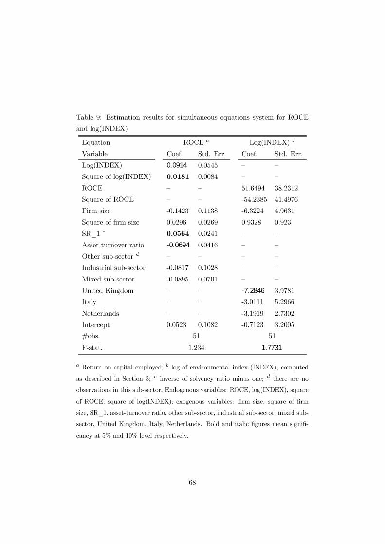
retained equation system are reported in Tables 911.
Tables 911 about here
Let us consider Þrstly the economic equations (ROCE, ROE, and ROS).
We observe that the environmental index (both its linear and square terms)
has a positive and signiÞcant (at 10% and 5% level, respectively) effect
on ROCE but has no effect on the other economic performance indica-
tors. In Figure 6, we plot the estimated relationship between ROCE and
log(INDEX). The graph displays a U-shape curve. However, the increas-
ing part of the curve is not robust due to few observations. Then only the
decreasing part might be considered. This decreasing part shows a relation
with a negative Þrst derivative and a positive second derivative. This Þnding
seems more consistent with traditionalist reasoning about the relationship
between environmental and economic performance, which predicts the re-
lationship to be uniformly negative (see Section 2, Figure 1). This result
shows evidence of a trade-off between return on capital employed and envi-
ronmental performance. Implications of this result will be discussed later.
Figure 6 about here
Firm size has no signiÞcant inßuence on our three economic performance
variables. SR_1 in the ROCE equation is positive and signiÞcant at 5%
level. This is however inconsistent with theory, since ROCE is theoretically
already controlled for gearing. It is insigniÞcant in other economic equations.
38
For the asset-turnover ratio, we obtain a negative and signiÞcant impact at
10% level on ROCE, and a positive and signiÞcant impact at 5% level on
ROS while no relationship is found for ROE.
Concerning sub-sector dummies in the economic equations (remember
that country dummies are excluded from this equation for identiÞcation
purpose), industrial and mixed sub-sector have a signiÞcant effect at 10%
and 5%, respectively, on ROS. This effect is negative. Then Þrms in these
two sub-sectors have less return on sales than Þrms in the cultural sub-
sectors (reference), all other things being equal.
Now we discuss the results following from the environmental equation.
There is no evidence of signiÞcant relationship between economic perfor-
mance variable and the log of the environmental index. The same con-
clusion applies to Þrm size. About country dummies (sub-sector dummies
are excluded from the environmental equation), United Kingdom located
Þrms have negative and signiÞcant effect on log(INDEX) in the system with
ROCE (10% level) and in the system with ROS (5% level). Italy located
Þrms inßuence positively and signiÞcantly at 5% level log(INDEX) in the
system with ROS. As a result, from an environmental point of view, we
can conclude that United Kingdom and Italy located Þrms perform respec-
tively less and more than Germany ones. This may indicate a selection bias
towards better-performing Þrms in Italy (likely as a result of self-selection).
In Tables 911, we also report the F-statistics to test the signiÞcancy
of each equation in each system. The environmental equation is signiÞcant
at 5% level in all systems, excepted for the system deÞned by ROCE and
log(INDEX) which is signiÞcant at 10% level. The economic equation is
signiÞcant only for ROS.
6 Conclusions and Recommendations
As noticed in Section 3, the data sample covers a low proportion of Italian
Þrms. We also know that the environmental regulation is less stringent in
Italy than in other countries (notably Germany). So the better environ-
mental performance of Italian Þrms (in both separated and simultaneous
regressions) is an unexpected result and we think that it should be treated
39
carefully.
The hypothesis H1 seems to be conÞrmed, since, relative to Germany,
other country dummies have a positive and signiÞcant effect on economic
performance in the pooled regressions. This can be interpreted in a way
that a strong country effect for economic performance exists, which can
be interpreted as higher costs of environmental regulation since economic
performance is relatively lower in Germany than in the other three countries.
However, it has to be noted that most country effects become insigniÞcant
in the random effects model (except for the UK), thus indicating that any
reduction of competitiveness through stringent environmental regulation has
to be considered carefully with regard to other (random) inßuences on the
economic performance of Þrms.
With regard to environmental performance, H1 seems to be conÞrmed
in that there are some signiÞcant positive country effects for COD, SO2
and the environmental index (i.e. signiÞcant and positive coefficients for
the Netherlands and the United Kingdom). This can be interpreted as
a better environmental performance of Þrms in Germany, relative to the
other countries. Consistent with this is also the reversal of the coefficient
signs in the case of the environmental index for the UK(since for the index,
high values represent good performance, whereas the inverse is the case for
the individual environmental performance variables). However, the country
inßuences found for Italy for the index and for COD are inconsistent with
H1. Therefore, (i) the inßuence of stringent environmental regulation on
the environmental performance of Þrms seems to be sensitive to the speciÞc
measure for environmental performance and (ii) in the case of Italy, the
selection of Þrms may have been biased towards the better environmental
performers.
The Hypothesis H2 seems to be conÞrmed only to some degree, since the
analysis found positive and signiÞcant coefficients for the United Kingdom
and the Netherlands in the case of all economic performance variables in the
pooled regression. Given that the Netherlands and the UK are rated high-
est with regard to the use of ßexible (i.e. economic) instruments in Table 1
this result is as expected. However, it has again to be noted that (i) most
effects become insigniÞcant in the random effects model and that (ii) in the
40
pooled regressions also Italy has a signiÞcant country effect on ROE, which is
counter to the ranking in Table 1. Therefore, economic instruments seem to
have a less negative/more positive inßuence on economic performance, but
again, random effects seem to have some inßuence. In addition to this, there
is of course some interdependence between hypotheses H1 and H2. In sum-
mary, the relationship between environmental and economic performance as
predicted in H1 and H2 only holds in direct comparisons of Germany and
the UK for ROCE, COD and the environmental index (based on the random
effect model).
Hypothesis H3 is conÞrmed in the case of the environmental performance
variables. The Þndings regarding sub-sector inßuences on environmental
performance variables are consistent with the strong sub-sector effect found
by Berkhout et al. (2001b). However, the fact that some of the sub-sector
inßuences become insigniÞcant in the random effects model indicates that
do not account for unobservable Þrm heterogeneity in the pooled regression
might have artiÞcially increased signiÞcance levels for sub-sector inßuence
in some cases. Regarding the economic performance variables, no signiÞcant
sub-sector effect could be found.
Regarding hypothesis H4 it was found that there is almost no signiÞcant
effect of Þrm size on either economic or environmental performance, the
only exception being a positive and signiÞcant effect of the linear term for
Þrm size on ROE in the case of pooled regression, which however becomes
insigniÞcant for the random effects model. This conÞrms H4 with regards to
economic performance (where no signiÞcant effect was expected), but also
indicates that there seems to be no substantial difference in environmental
performance between smaller and larger Þrms. This means that the often
perceived differences between SMEs and large Þrms are likely smaller than
stated in the literature and that (given that the insigniÞcance of Þrm size on
economic performance was conÞrmed) the a priori assumption that smaller
Þrms tend to have a less positive relationship between environmental and
economic performance has to be considered carefully. At least the data anal-
ysed here does not provide an indication that smaller Þrms cannot achieve as
easily economies of scale in environmental management as larger ones. Dif-
ferences of cross-sectional variances were only analysed qualitatively based
41
on scatterplots for 95-97 averages.19 Scatterplots indicate decreasing vari-
ance with increasing Þrm size for ROS, ROCE, COD, NOx and SO2. This
might indicate a higher variation in the relationship between environmental
and economic performance for smaller Þrms.
What the separated regressions did not take into account is the possible
endogeneity of the relationship between environmental and economic perfor-
mance. The mutual inßuences between environmental and economic perfor-
mance were therefore addressed by means of three simultaneous equations
systems. For these, it was found that the results -for the system with ROCE
as economic performance variable, only- were more consistent with the tra-
ditionalist view, than with the revisionist perspective on the relationship
between environmental and economic performance. However results are not
very clear-cut, in that similar results could not be found for the systems
with ROS and ROE as economic performance variables, respectively.
The important question is of course at this point, what these Þndings im-
ply for the relationship between environmental and economic performance.
There seem to be two main conclusions. Firstly, there seems to be consid-
erable inßuence of noise in the data. Environmental and economic perfor-
mance can be inßuenced by many more factors than those included in the
theoretical framework. Although it was attempted to keep the inßuence of
these other factors constant, we have no deÞnite benchmark indicating to
which degree this was achieved. Given that the signal of environmental per-
formance as an inßuence on economic performance is small, it would be de-
sirable to utilize, in a next research step, more direct measures capturing the
relationship between environmental and economic performance. One way to
achieve this could e.g. be the separation of some green proÞt component
from the overall economic performance of a Þrm. Secondly, even though
some of the Þndings for the simultaneous equation systems Þt better with
traditionalist reasoning about the relationship between environmental and
economic performance, which predicts the relationship to be uniformly neg-
ative, both theoretical models presented in the beginning of the paper are
not well-supported by the results. This element of inconclusiveness in the
19Scatterplots are available from the authors on request.
42
results will likely be reduced if a more direct measure of that part of a Þrms
overall proÞtability which is the result of its environmental performance (or
improvements thereof) can be devised and applied.
43
7 Appendix
7.1 Appendix 1: Variable deÞnition and descriptive statis-tics
Table A1: DeÞnition of variables.
Variable Description Typea
Economic ROCE Return on capital employed cont.
performance ROE Return on equity cont.
ROS Return on sales cont.
COD Emissions of chemical oxygen demand cont.
Environmental (tonnes per tonne, t/t)
performance SO2 Emissions of sulphur dioxide (t/t) cont.
NOx Emissions of nitrogen oxides (kilo t/t) cont.
Log(INDEX) Log of the environmental index (dimensionless) cont.
Firm size Number of employees (thousand) int.
Control SR_1 Inverse of solvency ratio minus one (%) cont.
variables Asset-turnover Inverse of the turnover-to-asset ratio
ratio (Great Britain Pounds GBP/GBP) cont.
United Kingdom United Kingdom located Þrm dum.
Country Italy Italy located Þrm dum.
Netherlands Netherlands located Þrm dum.
Germany Germany located Þrm dum.
Cultural Newsprint, magazine-grade, and dum.
graphics Þne paper (reference)
Sub-sector Industrial Packaging corrugated and other boards dum.
Mixed Cultural and industrial paper production dum.
Other Other paper production dum.
a cont., int., and dum. mean respectively continuous type, integer type (treated in
the estimations as continuous) and dummy type variables.
44
Table A2: Descriptive statistics for year 1995
Variable Mean Std.Dev. Min Max. #obs.
ROCE 0.155 0.217 -0.1254 1.043 32
ROE 0.1278 0.2088 -0.2713 0.7032 33
ROS 0.0422 0.0664 -0.0711 0.2321 33
COD 7.9413 8.5049 0.2902 27.2964 28
SO2 3.3497 9.559 0 49.1401 28
NOx 0.0020 0.0047 0 0.0256 30
INDEX 0.1449 0.3383 0.0008 0.9886 22
Log(INDEX) -4.3993 2.19 -7.138 -0.0115 22
Firm size 0.6873 0.6907 0.119 3.548 33
SR_1 2.7423 2.1846 0.2174 11.0048 33
Asset-turnover ratio 1.0285 0.919 0.4366 5.6249 33
United Kingdom 0.2571 0.4435 0 1 35
Italy 0.2 0.4058 0 1 35
Netherlands 0.2571 0.4435 0 1 35
Germany 0.2857 0.4583 0 1 35
Industrial 0.1714 0.3824 0 1 35
Cultural 0.4571 0.5054 0 1 35
Mixed 0.2571 0.4434 0 1 35
Other 0.1143 0.3228 0 1 35
45
Table A3: Descriptive statistics for year 1996
Variable Mean Std.Dev. Min Max. #obs.
ROCE 0.113 0.1552 -0.3641 0.5582 31
ROE 0.1326 0.2364 -0.514 0.7951 32
ROS 0.0502 0.0807 -0.1264 0.254 32
COD 9.9113 15.7274 0.3301 80.057 28
SO2 3.4133 10.105 0 51.9481 28
NOx 0.002 0.0056 0 0.3070 29
INDEX 0.139 0.3318 0.0007 0.9883 23
Log(INDEX) -4.5607 2.2535 -7.3214 -0.0118 23
Firm size 0.6913 0.7564 0.132 4.019 33
SR_1 2.3952 1.4604 0.3203 5.1162 32
Asset-turnover ratio 1.1476 0.7207 0.4187 3.5352 32
United Kingdom 0.2647 0.4478 0 1 34
Italy 0.2059 0.4104 0 1 34
Netherlands 0.2353 0.4306 0 1 34
Germany 0.2941 0.4625 0 1 34
Industrial 0.1765 0.387 0 1 34
Cultural 0.4412 0.504 0 1 34
Mixed 0.2647 0.4478 0 1 34
Other 0.1176 0.3270 0 1 34
46
Table A4: Descriptive statistics for year 1997
Variable Mean Std.Dev. Min Max. #obs.
ROCE 0.0982 0.0872 -0.1146 0.346 29
ROE 0.0776 0.2334 -0.8601 0.5338 32
ROS 0.0213 0.1213 -0.5316 0.1902 33
COD 41.3956 187.1874 0.4293 1082.353 33
SO2 2.4419 8.9888 0 49.6278 31
NOx 1.1192 4.8961 0 26.4546 33
INDEX 0.1189 0.3028 0.0007 0.9879 28
Log(INDEX) -4.4283 2.0578 -7.26 -0.0121 28
Firm size 0.6273 0.6827 0.11 3.697 36
SR_1 2.2948 1.5828 0.2425 5.8823 33
Asset-turnover ratio 1.0452 0.5665 0.3792 2.9673 32
United Kingdom 0.2432 0.435 0 1 37
Italy 0.2432 0.435 0 1 37
Netherlands 0.2432 0.435 0 1 37
Germany 0.2703 0.4502 0 1 37
Industrial 0.1892 0.3971 0 1 37
Cultural 0.4324 0.5022 0 1 37
Mixed 0.2432 0.435 0 1 37
Other 0.1351 0.3466 0 1 37
Appendix 2: Maximum likelihood estimation of the separatedequations
To simplify notation, we denote x = [x, z], and β = [β0,γ0]0 the proper
stacked format of time-varying as well as time-invariant regressors and re-
lated vector of parameters, where the intercept term is excluded by tacking
deviations from the overall sample mean. Then, on the assumption that
u ∼ N(0,Ω), with
Ω = E(uu0) = σ2µ(IN⊗JT ) + σ2
λ(JN⊗IT ) + σ2εINT , (9)
47
the joint log likelihood of the observations y, conditional on the values of x
can be expressed as
L(y|x, β,σ2, ρ,ω) = −NT2
¡ln 2π + lnσ2
¢− 1
2σ2(y∗−x∗β)
0(y∗−x∗β)
−1
2ln [det (ξ1BN + ξ2BT + ξ3W)] , (10)
where ξ1 = (1− ρ− ω − Tρ), ξ2 = (1− ρ− ω −Nω), ξ3 = (1− ρ− ω); and
σ2 = σ2µ+σ2
λ+σ2ε, ρ = σ2
µ/σ2, ω = σ2
λ/σ2, ξ3 = σ2
ε/σ2. The matrix notations
are completed as BN = (IN − JNN ) ⊗ (JN
T ), BT = JNN ⊗ (IT − JT
T ), W =
(IN− JNN )⊗(IT − JT
T ), y∗ = (Ω∗)−1/2y and x∗ = (Ω∗)−1/2x, where (Ω∗)−1/2
is the squared root matrix which yields the proper spectral decomposition
representation of Ω (Wansbeek and Kapteyn, 1982, 1983).
The log likelihood function can be concentrated in terms of the param-
eters ρ and ω by Þxing these and maximizing out β and σ2. The GLS
estimate that maximizes β is given by
RSS(ρ,ω) = minβ∈Θ
(y∗−x∗β)0(y∗−x∗β)
and the value of σ2 which maximizes the log likelihood conditional on ρ and
ω is
σ2 =RSS(ρ,ω)
NT.
As a result, the concentrated log-likelihood function is a function only in
arguments ρ and ω and can be maximised with respect those parameters by
grid search or steepest ascent methods. For details on this computation, see
Nerlove (1999).
8 References
Amemiya, T. (1971) The Estimation of the Variance in a Variance-Components
Model, International Economic Review, 12, pp. 113.
Arnold J., Hope, T., and Southworth, A. (1985) Financial Accounting,
Prentice-Hall, London.
Baltagi, B.H. (1995) Econometric Analysis of Panel Data, John Wiley and
Sons, Chichester, New York.
48
Berkhout, F., Hertin, J., Tyteca, D., Carlens, J., Olsthoorn, X., van
Druinen, M., van der Woerd, F., Azzone, G., Noci, G., Jasch, C.,
Wehrmeyer, W., Wagner, M., Gameson, T., Wolf, O., and Eames, M.
(2001a) MEPI — Measuring Environmental Performance of Industry,
Final report and appendices submitted to the European Commission,
DG XII, February.
Accessible at http://www.environmental-performance.org/outputs/index.php.
Berkhout F., Hertin, J., Carlens, J., Tyteca, D., Olsthoorn, X., Wagner,
M. and Wehrmeyer, W. (2001b) Green-ness Can Be Measured, Eu-
ropean Business Forum, 6, pp. 42-47.
Bradford, D. (2000) Motivating SMEs Towards Improved Environmental
Performance, The IPTS Report no. 41, JRC - Seville, February, pp.
25-29.
Breusch, T.S. and Pagan, A.R. (1980) The Lagrange Multiplier Test and
Its Applications to Model SpeciÞcation in Econometrics, Review of
Economic Studies, 47, pp. 239-253.
Clift, R. (1998) Relationships Between Environmental Impacts and Added
Value along the Supply Chain, Invited Lecture at the 2nd International
Conference on Technology, Policy and Innovation, Lisbon, August.
Cohen, M., Fenn, S., and Naimon, J. (1995) Environmental and Financial
Performance: Are They Related?, Working Paper, Owen Graduate
School of Management, Vanderbilt University.
EIM (1997) The European Observatory for SMEs - Fifth Annual Report,
Luxembourg: EUR-Op and Zoetermeer: EIM Small Business Research
and Consultancy.
Esty, D.C. and Porter, M.E. (2001) Measuring National Environmental
Performance and Its Determinants, in: Porter, M.E. and Sachs, J.
(eds.) The Global Competitiveness Report 2000, Oxford University
Press, New York, pp. 60-75.
49
Ganzleben, C. (1998) The Production Processes Employed by the Pulp and
Paper Industry, Working Papers in Geography WPG 99-5, School of
Geography, University of Oxford, Oxford.
Gordon, J. (1994) Environmental Policy in Britain and Germany: Some
Comparisons, European Environment, June, pp. 9-12.
Greene, W.H. (2000) Econometric Analysis (4th ed.), Prentice-Hall, Lon-
don.
Hart, S.L. and Ahuja, G. (1996) Does it Pay to Be Green? An Empiri-
cal Examination of the Relationship between Emission Reduction and
Firm Performance. Business Strategy and the Environment, 5, pp.
30-37.
Heidemark, P. and Backman, M. (1999) Environmental Management in
Swedish Manufacturing Industries, Paper presented at the 1999 Eco-
Management and Auditing Conference, University of Leeds, 1-2 July.
Henriques, I. and Sadorsky, P. (1996) The Determinants of an Environ-
mentally Responsive Firm : An Empirical Approach, Journal of En-
vironmental Economics and Management, 30, pp. 381-395.
Houghton, J.T., Meira Filho, L.G., Bruce, J., Lee, H., Callander, B.,
Haites, E., Harris, N., and Maskell, K. (eds.) (1995) Climate Change
1994. Radiative Forcing of Climate Change and Evaluation of the
IPCC IS92 Emission Scenarios, Cambridge University Press, Cam-
bridge.
Jaggi, B. and Freedman M. (1992) An Examination of the Impact of Pollu-
tion Performance on Economic and Market Performance of Pulp and
Paper Firms, Journal of Business Finance and Accounting, 19(5), pp.
697-713.
James, P., Prehn, M., and Steger, U. (1997) Corporate Environmental Man-
agement in Britain and Germany, Anglo-German Foundation, Lon-
don.
50
Luken, R., Kumar, R., and Artacho-Garces, J. (1996) The Effect of Envi-
ronmental Regulations on Industrial Competitiveness of Selected In-
dustries in Developing Countries, Paper Presented at the 5th Greening
of Industry International Conference: Global Restructuring: a Place
for Ecology?, Heidelberg, Germany, November 24-27.
Lumby, S. (1991) Investment Appraisal and Financial Decisions (5th ed.),
Chapman-Hall, London.
Meffert, H. and Kirchgeorg, M. (1998) Marktorientiertes Umweltmanage-
ment (Market-oriented environmental management) (3rd. ed.), Stuttgart.
Morris, D.J. and Hay, D.A. (1991) Industrial Economics and Organisation
— Theory and Evidence, Oxford University Press, Oxford.
Moschandreas, M. (1994) Business Economics, Routledge, London.
Myers, S.C. and Brealey, R.A. (1988) Principles of Corporate Finance (3rd
ed.), McGraw-Hill, New York.
Nerlove, M. (1999) Analysis of Panel Data, mimeo, University of Maryland.
Olsthoorn, X., Tyteca, D., Wehrmeyer, W., and Wagner, M. (2001) Using
Environmental Indicators for Business? A Literature Review and the
Need for Standardisation and Aggregation of Data, Journal of Cleaner
Production, forthcoming.
Peattie, K. and Ringer, A. (1994) Management and the Environment in
Germany and the UK: A Comparison, European Management Journal,
June, pp. 216-225.
Pendlebury, M. and Groves, R. (1999) Company Accounts — Analysis, Inter-
pretation and Understanding (4th ed.), International Thomson Busi-
ness Press, London.
Porter, M. (1991) Americas Green Strategy, Scientific American, 264(4),
p. 168.
51
Porter, M. and Esty, D. (1998) Industrial Ecology and Competitiveness:
Strategic Implications for the Firm, Journal of Industrial Ecology,
2(1), pp. 35-43.
Porter, M. and van der Linde, C. (1995) Green and Competitive: End-
ing the Stalemate, Harvard Business Review, September-October, pp.
120-134.
Reid, W. and Myddelton, D.R. (1995) The Meaning of Company Accounts
(5th ed.), Gower, Aldershot.
Russo, M.V. and Fouts, P.A. (1997) A Resource-Based Perspective on
Corporate Environmental Performance and ProÞtability, Academy of
Management Journal, 2(3), pp. 534-559.
Schaltegger, S. and Figge, F. (1998) Environmental Shareholder Value,
WWZ/Sarasin Basic Report no. 54, Basel.
Schaltegger, S. and Figge, F. (2000) Environmental Shareholder Value:
Economic Success with Corporate Environmental Management, Eco-
Management and Auditing, 7(1), pp. 29-42.
Schaltegger, S. and Synnestvedt, T. (1999) The Forgotten Link Between
Green and Economic Success Environmental Management as the
Crucial Trigger between Environmental and Economic Performance,
Lueneburg and Oslo, University of Lueneburg and Norwegian School
of Management, September.
Schmalensee, R. (1989) Inter-Industry Studies of Structure and Perfor-
mance, in Schmalensee, R. and Willig, R.D. (eds.) (1989) Handbook
of Industrial Organization, Volume II, Elsevier Science Publishers, pp.
951-1009.
Schmidheiny, S. (1992) Changing Course, MIT Press, Cambridge, Mas-
sachussetts.
Silverman, B.W. (1986) Density Estimation for Statistics and Data Anal-
ysis, Chapman & Hall, London.
52
Tyteca, D. (1999) Sustainability Indicators at the Firm Level Pollution
and Resource Efficiency as a Necessary Condition towards Sustainabil-
ity, Journal of Industrial Ecology, 2(4), pp. 183-197.
Tyteca, D., Carlens, J., Berkhout, F., Hertin, J., Wehrmeyer, W., and
Wagner, M. (2001) Corporate Environmental Performance Evaluation:
Evidence from the MEPI Project, Business Strategy and the Environ-
ment, forthcoming.
Wagner, J. (1995) Firm Size and Job Creation in Germany, Small Business
Economics, 7, pp. 469-474.
Wagner, M., Wehrmeyer, W., and Carlens, J. (2001) The Relationship be-
tween Environmental and Economic Performance of Firms and the
Inßuence of ISO 14001 and EMAS: An Empirical Analysis, in: Con-
ference Proceedings of the 2001 Eco-Management and Auditing Con-
ference. Shipley: ERP Environment, pp. 286-293.
Walley, N. and Whitehead, B. (1994) Its not Easy Being Green, Harvard
Business Review, May-June, pp. 46-52.
Wansbeek, T., Kapteyn, A. (1982) A Simple Way to Obtain the Spectral
Decomposition of Variance Components Models for Balanced Data,
Communications in Statistics, A11, pp. 21052112.
Wansbeek, T., Kapteyn, A. (1983) A Note on Spectral Decomposition and
Maximum Likelihood Estimation of ANOVA Models with Balanced
Data, Statistics and Probability Letters, 1, pp. 213215.
Wätzold, F., Bültmann, A., Eames, M., Lulofs, K.R., and Schucht, S.
(2001) EMAS and Regulatory Relief in Europe: Lessons from National
Experience, European Environment, 11(1), pp. 37-48.
WEF, YCELP, CIESIN (World Economic Forum, Yale Center for Environ-
mental Law and Policy, and CIESIN) (2001) 2001 Environmental Sus-
tainability Index (http://www.ciesin.columbia.edu/indicators/ESI), Jan-
uary, accessed 20 July 2001.
53
WEF, YCELP, CIESIN (World Economic Forum, Yale Center for Environ-
mental Law and Policy, and CIESIN) (2000) Pilot Environmental Sus-
tainability Index (http://www.ciesin.columbia.edu/indicators/ESI), ac-
cessed 20 July 2001.
Wehrmeyer, W and Tyteca, D. (1998) Measuring Environmental Perfor-
mance for Industry: from Legitimacy to Sustainability? The Interna-
tional Journal of Sustainable Development and World Ecology, 5, pp.
111-124.
You, J.-I. (1995) Small Firms in Economic Theory, Cambridge Journal of
Economics, 19, pp. 441-462.
54
Env. Perf.
Econ. Perf.
Env. Perf.
Econ. Perf.
(a) (b)
Figure 1: (a) the traditionalist view; (b) the revisionist view.
Influencing factors:- corporate environmental strategies/management- country location/ environmental regulation- processes operated- industry market structure / sector membership- firm size
Environmental performance Economic performance
Figure 2: Initial model for the interaction of environmental and economic
performance.
55
Influencing factors:- corporate environmental
strategies/management- country location/
environmentalregulation
- processes operated- firm size- industry market structure
/ sector membership
Environmentalperformance
Economicperformance
Additional factors:- investors- return
expectations- changing market
conditions- cyclic nature of
industries- capital intensity
of industries
Figure 3: Expanded model for the interaction of environmental and eco-
nomic performance.
56
Den
sity
.INDEX
0 .5 1
0
10
20
Figure 4: Kernel density estimate of INDEX for the pooled data. High
frequencies for extreme values are observed.
57
Den
sity
.Log(INDEX)
-8 -6 -4 -2 0 1
0
.05
.1
.15
.2
Figure 5: Kernel density estimate of log(INDEX) for the pooled data. Tri-
modal distribution underlying the environmental index. Positive values of
log(INDEX) displayed on the abscissa are due to graphical rescaling.
58
RO
CE
.Log(INDEX)
-7 -4 -2 -.2
-.2
0
.2
Figure 6: The relationship between ROCE and log(INDEX) obtained from
the estimation of the simultaneous equations system.
59
Table 1: Stringency of regulation and orientation towards economic instru-
ments in four countries
Country Germany Italy Netherlands UK
Stringency of regulation 1.82 0.25 1.53 0.99
(rank, 1 = highest) a (1) (4) (2) (3)
Use of ßexible instruments
(rank, 1= highest) b (3) (4) (1) (2)
Transparency of regulation 4.1 2.8 4.4 4.5
(rank, 1= highest) c (3) (4) (2) (1)
Innovation through regulation 0.7 -0.50 1.34 1.18
(rank, 1= highest) d (3) (4) (1) (2)
Regulatory and management 1.34 0.08 0.75 1.54
indicator e (2) (4) (3) (1)
Regulatory regime 1.205 0.035 1.623 1.087
index f (2) (4) (1) (3)
a Data of the measure Stringency and consistency of environmental regulation,
in 2000 in WEF et al. (2001). b Ranking is based on authors assessment of
how much a country applies voluntary or economic instruments. c Data of the
measure Transparency and stability of environmental regulation, in 1999 in WEF
et al. (2000). d Data based on measure Degree to which environmental regulation
promotes innovation, measured in 2000 in WEF et al. (2001). e Data based on
Regulation and management indicator in WEF et al. (2001) which comprises of
the measure Stringency and consistency of environmental regulation, in 2000 in
WEF et al. (2001) as one component. f Data of the index is based on Esty and
Porter (2001). The index assesses stringency of standards, subsidies, regulatory
enforcement, regulatory structure, information and environmental institutions.
60
Table 2: Data distribution and EMS certiÞcation across countries (out of
total of Þrms in data set)
Year Germany Italy Netherlands UK Total
1995 Total 10 7 9 9 35
ISO 14001 1/10 0/7 1/8 0/9 2/34
1996 EMAS 3/10 0/7 0/8 1/9 4/34
Total EMS 3/10 0/7 1/8 1/9 5/34
ISO 14001 5/10 1/9 4/9 6/9 16/37
1997 EMAS 6/10 0/9 1/9 1/9 8/37
Total EMS 7/10 1/9 4/9 6/9 18/37
61
Table 3: Environmental performance indicators used (all per tonne of paper
produced)
Indicators name DeÞnition Relevance Unit Relevance
(MEPI, 2000) (MEPI, 2000) data sources
NOx emissions Emissions of AcidiÞcation, Kilo tonnes Environmental
(non-product NOx comprising local air per tonne reports veriÞed
outputs to air both, NO pollution of paper under EMAS or
of nitrogen and NO2, per annum ISO, pollution
oxides) per measured inventories,
production output as NO2 surveys
SO2 emissions Emissions of AcidiÞcation, Tonnes
(non-product outputs sulphur dioxide local air per tonne
to air of sulphur from production pollution of paper As above
dioxide) per processes per annum
production output
COD emissions Annual chemically COD of waste water Tonnes
(non-product determined (before treatment) per tonne
outputs to water demand of measures the of paper
(before treatment) oxygen from potential to per annum As above
of chemical oxygen waste water cause waterway
demand, COD) per contaminants pollution from
production output discharged de-oxygenation
62
Table 4: Separated estimation results for pooled (deviations from overall
means ) data for economic performance
Dependent variable ROCE a ROS b ROE c
Independent variable Coef. Std.Err. Coef. Std.Err. Coef. Std.Err.
Firm size 0.0688 0.0843 0.0531 0.037 0.3078 0.1295
Square of Þrm size -0.008 0.0197 -0.0066 0.0087 -0.045 0.0303
SR_1 d 0.0226 0.0133 -0.0166 0.0052 -0.01 0.0182
Asset-turnover ratio -0.0418 0.0226 0.035 0.001 -0.0176 0.0349
Other sub-sector -0.0364 0.0818 0.0041 0.0271 0.0018 0.0949
Industrial sub-sector 0.0062 0.0526 0.0033 0.0202 -0.0227 0.0706
Mixed sub-sector -0.0026 0.0389 -0.0246 0.0176 -0.0164 0.0617
United Kingdom 0.1979 0.0524 0.0432 0.0232 0.2002 0.081
Italy 0.1117 0.0729 0.0267 0.0325 0.2542 0.1137
Netherlands 0.1003 0.0577 0.0634 0.0256 0.2427 0.0894
#obs. 69 78 78
a Return on capital employed; b return on sales; c return on equity; d inverse of
solvency ratio minus one. Bold and italic Þgures mean signiÞcancy at 5% and 10%
level respectively.
63
Table 5: Random effects separated estimation results for economic per-
formance
Dependent variable ROCE a ROS b ROE c
Independent variable Coef. Std.Err. Coef. Std.Err. Coef. Std.Err.
Firm size 0.0706 0.1031 0.0383 0.0513 0.2725 0.1882
Square of Þrm size -0.0069 0.0241 -0.0025 0.012 -0.0304 0.0442
SR_1 d 0.012 0.017 -0.024 0.0064 -0.0888 0.0275
Asset-turnover ratio -0.0468 0.0257 0.0104 0.0115 -0.0588 0.0383
Other sub-sector -0.0487 0.104 -0.0131 0.0447 -0.0864 0.1711
Industrial sub-sector 0.0256 0.0667 0.004 0.0315 0.0717 0.12
Mixed sub-sector -0.0014 0.0494 -0.0292 0.0291 -0.0101 0.111
United Kingdom 0.1985 0.0653 0.0542 0.0358 0.1838 0.1354
Italy 0.1214 0.0911 0.0443 0.0497 0.3007 0.1869
Netherlands 0.0941 0.0725 0.0566 0.0396 0.1396 0.1515
Full log-likelihood 12.66 86.5 -12.34
#obs. 69 78 78
Breusch-Pagan test e
Þrm effect 0.2251 9.605 5.374
year effect 0.3389 0.4545 0.4158
Þrm & year effects 0.564 10.06 5.789
a Return on capital employed; b return on sales; c return on equity; d inverse of
solvency ratio minus one; e Breusch and Pagans (1980) test is a Lagrange-multiplier
test. Bold and italic Þgures mean signiÞcancy at 5% and 10% level respectively.
64
Table 6: Separated estimation results for pooled (deviations from overall
means) data for environmental performance
Dependent variable NOx a SO2b COD c
Independent variable Coef. Std.Err. Coef. Std.Err. Coef. Std.Err.
Firm size -1.584 1.613 6.576 5.659 -1.962 2.293
Square of Þrm size 0.3827 0.3974 -1.81 1.377 0.6122 0.7321
Other sub-sector -0.3416 1.094 -3.849 3.764 0.5147 2.217
Industrial sub-sector 1.283 0.8628 -4.418 3.154 6.187 1.799
Mixed sub-sector 0.4239 0.9571 -6.824 3.449 11.93 1.761
United Kingdom 0.8729 0.9628 3.593 3.386 5.726 1.991
Italy -0.9709 1.22 3.094 5.28 -5.229 2.033
Netherlands -0.7865 0.9927 9.552 3.45 5.706 2.037
#obs. 81 72 78
a Emissions of nitrogen oxides per production output, b emissions of sulphur dioxide
per production output, c emissions of chemical oxygen demand per production
output. Bold and italic Þgures mean signiÞcancy at 5% and 10% level respectively.
65
Table 7: Random effects separated estimation results for environmental
performance
Dependent variable NOx a SO2b COD c
Independent variable Coef. Std.Err. Coef. Std.Err. Coef. Std.Err.
Firm size -1.384 1.889 5.542 5.388 -2.184 3.166
Square of Þrm size 0.3403 0.4651 -1.557 1.308 0.5637 0.7725
Other sub-sector -0.3016 1.312 -4.023 3.811 0.3158 3.689
Industrial sub-sector 1.31 1.034 -4.543 3.197 6.047 2.955
Mixed sub-sector 0.439 1.147 -6.912 3.501 11.83 2.918
United Kingdom 0.9256 1.153 3.385 3.412 5.415 3.148
Italy -0.8898 1.449 2.645 5.29 -5.483 3.249
Netherlands -0.7206 1.185 9.283 3.463 5.421 3.239
Full log-likelihood -239.6 -252.2 -231.1
#obs. 81 72 78
Breusch-Pagan testd
Þrm effect 1.05 67.76 60.97
year effect 0.14 1.429 1.146
Þrm & year effects 1.19 69.19 62.12
a Emissions of nitrogen oxides per production output; b emissions of sulphur dioxide
per production output; c emissions of chemical oxygen demand per production
output; d Breusch and Pagans (1980) test is a Lagrange-multiplier test. Bold and
italic Þgures mean signiÞcancy at 5% and 10% level respectively.
66
Table 8: Separated estimation results for the environmental index
(log(INDEX))
Pooled regression Random effect regression
Independent variable Coef. Std.Err. Coef. Std.Err.
Firm size -0.9117 1.084 -0.4559 0.8553
Square of Þrm size 0.0711 0.242 0.0168 0.1927
Other sub-sector 0.1239 0.9149 0.2184 1.413
Industrial sub-sector -0.8873 0.514 -0.758 0.769
Mixed sub-sector -1.245 0.5714 -1.132 0.8762
United Kingdom -2.832 0.6869 -2.505 0.8859
Italy 3.658 0.9681 4.082 1.21
Netherlands -0.2405 0.7002 0.0804 0.9028
Full log-likelihood -79.56
#obs. 57 57
Breusch-Pagan testa
Þrm effect 48.25
year effect 1.403
Þrm & year effects 49.66
a Breusch and Pagans (1980) test is a Lagrange-multiplier test. Dependent vari-
able: log(INDEX). Bold and italic Þgures mean signiÞcancy at 5% and 10% level
respectively.
67
Table 9: Estimation results for simultaneous equations system for ROCE
and log(INDEX)
Equation ROCE a Log(INDEX) b
Variable Coef. Std. Err. Coef. Std. Err.
Log(INDEX) 0.0914 0.0545
Square of log(INDEX) 0.0181 0.0084
ROCE 51.6494 38.2312
Square of ROCE -54.2385 41.4976
Firm size -0.1423 0.1138 -6.3224 4.9631
Square of Þrm size 0.0296 0.0269 0.9328 0.923
SR_1 c 0.0564 0.0241
Asset-turnover ratio -0.0694 0.0416
Other sub-sector d
Industrial sub-sector -0.0817 0.1028
Mixed sub-sector -0.0895 0.0701
United Kingdom -7.2846 3.9781
Italy -3.0111 5.2966
Netherlands -3.1919 2.7302
Intercept 0.0523 0.1082 -0.7123 3.2005
#obs. 51 51
F-stat. 1.234 1.7731
a Return on capital employed; b log of environmental index (INDEX), computed
as described in Section 3; c inverse of solvency ratio minus one; d there are no
observations in this sub-sector. Endogenous variables: ROCE, log(INDEX), square
of ROCE, square of log(INDEX); exogenous variables: Þrm size, square of Þrm
size, SR_1, asset-turnover ratio, other sub-sector, industrial sub-sector, mixed sub-
sector, United Kingdom, Italy, Netherlands. Bold and italic Þgures mean signiÞ-
cancy at 5% and 10% level respectively.
68
Table 10: Estimation results for simultaneous equations system for ROE
and log(INDEX)
Equation ROE a Log(INDEX) b
Variable Coef. Std. Err. Coef. Std. Err.
Log(INDEX) 0.0243 0.0649
Square of log(INDEX) 0.0037 0.0093
ROE 15.67 14.4732
Square of ROE 4.0698 6.9357
Firm size 0.083 0.1273 -3.4321 7.5529
Square of Þrm size -0.0094 0.0320 0.4101 1.3669
SR_1 c 0.0203 0.0237
Asset-turnover ratio -0.0201 0.0364
Other sub-sector 0.04 0.1271
Industrial sub-sector -0.1577 0.1029
Mixed sub-sector -0.1054 0.0708
United Kingdom -3.7089 4.1119
Italy 2.2596 5.9312
Netherlands -0.5373 4.246
Intercept 0.0506 0.1169 -2.9146 5.8569
#obs. 57 57
F-stat. 1.2063 5.6446
a Return on equity; b log of environmental index (INDEX) computed as described
in Section 3; c inverse of solvency ratio minus one. Endogenous variables: ROCE,
log(INDEX), square of ROCE, square of log(INDEX); exogenous variables: Þrm
size, square of Þrm size, SR_1, asset-turnover ratio, other sub-sector, industrial
sub-sector, mixed sub-sector, United Kingdom, Italy, Netherlands. Bold Þgures
mean signiÞcancy at 5%.
69
Table 11: Estimation results for simultaneous equations system for ROS and
log(INDEX)
Equation ROS a Log(INDEX) b
Variable Coef. Std. Err. Coef. Std. Err.
Log(INDEX) -0.0089 0.0175
Square of log(INDEX) -0.0006 0.0025
ROS 13.1204 10.005
Square of ROS -81.5832 51.6915
Firm size 0.0069 0.0347 -0.7053 1.5067
Square of Þrm size -0.0017 0.0084 0.0296 0.314
SR_1 c -0.00002 0.007
Asset-turnover ratio 0.0329 0.0131
Other sub-sector 0.0633 0.04
Industrial sub-sector -0.0586 0.0333
Mixed sub-sector -0.0681 0.0228
United Kingdom -2.1825 0.9803
Italy 3.8307 1.224
Netherlands 0.0173 0.9937
Intercept -0.0067 0.0359 -3.5637 1.3018
#obs. 57 57
F-stat. 4.068 11.1917
a Return on sales; b log of environmental index (INDEX), computed as described
in Section 3; c inverse of solvency ratio minus one;. Endogenous variables: ROCE,
log(INDEX), square of ROCE, square of log(INDEX); exogenous variables: Þrm
size, square of Þrm size, SR_1, asset-turnover ratio, other sub-sector, industrial
sub-sector, mixed sub-sector, United Kingdom, Italy, Netherlands. Bold and italic
Þgures mean signiÞcancy at 5% and 10% level respectively.
70