Banco de México

Documentos de Investigación

Banco de México

Working Papers

N° 2018-07

Determinants of FDI Attract ion in the ManufacturingSector in Mexico, 1999-2015.

June 2018

La serie de Documentos de Investigación del Banco de México divulga resultados preliminares detrabajos de investigación económica realizados en el Banco de México con la finalidad de propiciar elintercambio y debate de ideas. El contenido de los Documentos de Investigación, así como lasconclusiones que de ellos se derivan, son responsabilidad exclusiva de los autores y no reflejannecesariamente las del Banco de México.

The Working Papers series of Banco de México disseminates preliminary results of economicresearch conducted at Banco de México in order to promote the exchange and debate of ideas. Theviews and conclusions presented in the Working Papers are exclusively the responsibility of the authorsand do not necessarily reflect those of Banco de México.

Fel ipe J . FonsecaBanco de México

I rv ing Llamosas-RosasBanco de México

Determinants of FDI Attract ion in the Manufactur ingSector in Mexico, 1999-2015.

Abstract: Using an up-to-date database that improves the identification of the destination of theForeign Direct Investment (FDI) among Mexican states and spatial panel econometric models thatquantify the potential interactions and spillover effects, we analyze the main characteristics that helpunderstand the regional distribution of manufacturing FDI in Mexico. Our main findings indicate thepresence of a positive spatial relationship among states' FDI; for example, a higher investment creates apositive spillover effect on neighboring states' FDI and positive direct and indirect effects of humancapital, agglomeration and states' fiscal margin. Based on the results of this research, key implicationsfor public policy oriented to strengthen the FDI reside in increasing the average education level andimproving tax revenue of Mexican states.Keywords: FDI, spatial panel econometric models, spillover effectsJEL Classification: C21, C23, R12

Resumen: Utilizando una base de datos actualizada que mejora la identificación del destino de laInversión Extranjera Directa (IED) entre los estados de México así como modelos econométricosespaciales en panel para cuantificar las interacciones potenciales y efectos de derrame, analizamos lascaracterísticas que ayudan a entender la distribución de la IED manufacturera en México. Nuestrosresultados principales indican la presencia de relaciones positivas espaciales entre la IED de los estados;por ejemplo, una inversión más alta crea efectos de derrame en la IED de los estados vecinos y efectosdirectos e indirectos positivos en capital humano, aglomeración y autonomía fiscal estatal. Con base enlos resultados de esta investigación, las implicaciones clave de política pública orientada a fortalecer laIED residen en incrementar el nivel promedio de educación y mejorar la recaudación fiscal en losestados de México.Palabras Clave: IED, panel espacial, modelo econométrico, efectos de derrame

Documento de Investigación2018-07

Working Paper2018-07

Fel ipe J . Fonseca †

Banco de MéxicoI rv ing L lamosas -Rosas ‡

Banco de México

† Dirección General de Investigación Económica. Email: ffonseca@banxico.org.mx. . ‡ Dirección General de Investigación Económica. Email: illamosasr@banxico.org.mx.

1

1 Introduction

Which characteristics drive Foreign Direct Investments (FDI) into one particular region? Do

regions compete in order to obtain those investments? Or does a particular FDI help to

increase the amount of investment in neighbor states? These questions are of particular

importance in a developing economy like Mexico since FDI helps to improve the economic

conditions of the recipient region and its surroundings (Coughlin and Segev, 2000).

Foreign Direct Investment gives the opportunity to developing countries (among other

things) to facilitate the access to developed countries’ markets and global production systems

through technology, productive supply chains and other intangible assets unavailable at

accessible prices in the local economy (UNCTAD, 2006). In the Mexican case, for example,

during the 1999-2015 period FDI accounted for, on average, 12.6 percent of the total gross

capital formation, and 2.7 percent with respect to total GDP. Also, the literature has identified

FDI as an important vehicle for technology and knowledge transfer through spillover effects.1

Since FDI is an important source of financial resources that help to improve the economic

activity in the region, the states can offer favorable conditions to investors in order to acquire

its benefits and to enhance job creation and economic growth. That is why a better

understanding of the determinants of FDI attraction helps to shape future public policy

strategies towards regional development (Jordaan, 2008). With an up-to-date database on the

distribution of FDI at the state level, the methodology of which has been recently revised by

the Ministry of Economy, and using spatial econometric techniques, we analyze the regional

localization patterns of FDI in the manufacturing industry in Mexico during the 1999-2015

period. We focus on this sector because it accounts for about 50 percent of the total inward

FDI during the considered period.

1 See, for example, Borensztein et al. (1998), Durham (2004) and Li and Liu (2005).

2

By applying a panel data Spatial Durbin Model (SDM), the main results of the study are: (i)

there is a positive spillover effect on the attraction process of manufacturing FDI across states

and the estimated spatial effect indicates that for an increase of 10% of manufacturing FDI

in state’s i neighbors, its FDI manufacturing flows will increase, on average, between 2.6%

and 4.3%; (ii) variables such as agglomeration,2 infrastructure and schooling show a positive

impact as a factor of FDI manufacturing attraction; (iii) we include an indicator of fiscal

incentives (fiscal margin), which has a positive impact on FDI flows and it is worth mention

that this is a novel result in the literature for the Mexican case; (iv) from a methodological

point of view -and in the spirit of LeSage and Pace (2009)’s-, the interpretation of the

estimated parameters is based on the decomposition of the impact effects, both direct and

indirect. This enables us to get a richer interpretation of the variable impacts regarding not

only of the own states’ characteristics but also in terms of their neighbors.

With these results, we can infer that manufacturing FDI is attracted to states with higher

educated population, larger telecommunication infrastructure, and with a higher ratio of

workers employed in the manufacturing sector. This result, along with the indirect impacts

found on the same variables, implies that the manufacturing FDI flows to a State depend, in

general, not only of its own characteristics but also on those of the neighboring states, thus

generating a clustering-type dynamic (Porter, 2003).

Moreover, these results along with those novel findings regarding fiscal margin variable

(both direct and indirect), support the argument. Regarding public policies aimed at

increasing flows of this type of investment, estimates suggest that, because of the positive

pattern of spatial dependence in the FDI localization process, the attraction of FDI should be

considered in a regional context and not only from a local perspective.

2 Following Glaeser (2010, p. 1), and broadly speaking, throughout the document we refer the concept of

agglomeration as: “the benefits that come when firms and people locate near one another together in cities

and industrial clusters”.

3

Besides this introduction, the document is organized as follows: section 2 contains

literature review. Sections 3 and 4 include an analysis of the regional and sectoral distribution

of FDI and the econometric model, respectively; section 5 shows the results and section 6

concludes.

2 Literature Review

Several studies, both at the international level and for the Mexican economy, have addressed

the estimation of the determinants of the attractiveness of FDI following one of two

estimation strategies (Jordaan, 2008). The first consists of studies using the number of new

foreign-owned firms (total or manufacturing) in the host economy as a dependent variable

by estimating conditional logit type models. The second category consists of taking the flows

or the stock of FDI in monetary units as a dependent variable against a set of regional

characteristics using a variety of econometric models, mainly panel type (fixed, random,

dynamic, etc.). Indeed, as Jordaan (2008, p. 396) pointed out: “…we can infer that those

regional characteristics that are significantly associated with the regional distribution of FDI

must play a role in the location process of new FDI”.

Moreover, the empirical literature identifies the following group of variables as the main

factors that influence the localization decision: regional demand, labor-related production

costs, physical infrastructure, human capital, the presence of agglomeration economies, and

public policies devoted to attract or facilitate new FDI projects. Of the factors above, those

related to public policy incentives are the most difficult to incorporate due to lack of the data

(Jordaan, 2008).

In addition to the previous set of variables, another branch of literature has pointed out that

FDI could be indeed spatially correlated. With this attribute, neighboring regions can affect

one another creating spillover effects or the so-called "third country/region effect". Coughlin

and Segev (2000) for example, pointed out that agglomeration economies and resource cost

could be considered as one of the sources of this kind of effects. In the case of the former,

4

agglomeration may lead to higher FDI in neighboring regions to the extent that its beneficial

effects spill over provinces, transcending administrative boundaries. Concerning the latter,

by raising resource costs in a region, FDI could make the cost structure in neighboring regions

more attractive in relative terms.3 In the next subsections, we describe the findings for the

topic under consideration at international level and for the Mexican economy, respectively.

2.1 International Evidence

Several studies have addressed the determinants of FDI attraction at a regional level. For the

case of advanced economies, by applying a conditional logit model at state level for the

United States for 1981-1983, Coughlin et al. (1991) found that, on one hand, agglomeration,

road infrastructure, per capita income and manufacturing density have a positive impact on

FDI, as well as higher unemployment rates and (surprisingly) unionization rates. On the other

hand, wages have a negative impact, while incentive policies have two effects: high state tax

rates impact negatively, while expenditures affect positively in order to attract FDI. In

another study for the United States, Bobonis and Shatz (2007) find similar results for

agglomerations (of foreign-owned property, plant, and equipment) and state policies,

particularly targeted policies like unitary taxation and state foreign offices during the 1985-

1999 period employing dynamic panel techniques. In the case of the United Kingdom, Hill

and Munday (1992), through the estimation of pooled OLS during 1980-1989, find that both

financial incentives and access to markets are important determinants of the regional

distribution of new FDI projects.

Crozet et al. (2004) analyze location choice for FDI firms in France during 1996-2005 period

using conditional logit models, finding a strong effect on agglomeration as a determinant of

location, and, on the other hand, little evidence in favor of public policy intervention through

3 In the context of a formal model, Hanson (1996) shows the effects of interactions between agglomerations

and cost resources (wages) in the case of the garment industry in Mexico. Although the author does not

consider FDI in his analysis, the model is useful to describe how external economies lead to agglomeration

processes.

5

fiscal incentives. For the European regions, Casi and Resmini (2014) results for the 2005-

2007 period, through the estimation of a cross section spatial lag model indicate that

infrastructure, market accessibility, labor force quality, governance, and agglomeration exert

a positive impact on attracting FDI. Moreover, they find a positive spatial effect. Jones and

Wren (2016), in the case of Great Britain, find different patterns of allocation between sectors

using Markov-transition matrix between 1996 and 2005. In particular, they find that services,

in general, differ from the location process of manufacturing, including those forward-linked

to manufacturing industries.

Concerning emerging economies, Coughlin and Segev (2000)4, using a cross section spatial

error model (SEM) to analyze cumulative FDI distribution across Chinese provinces for the

1990-1997 period, find that the domestic market, productivity indicators, and location in

coastal regions have a positive impact on FDI. Wages and illiteracy rates, on the other hand,

are negatively correlated with FDI, while the effect of infrastructure is ambiguous (not

statistically significant). Concerning to the spatial process, they find that a region’s FDI is

positively associated with FDI into neighboring regions, through the error term. Furthermore,

and for the Chinese regions too, Cheng and Kwan (2000) find similar results for wages,

regional GDP, and infrastructure in the period 1985-1995 with dynamic panel methodologies.

Moreover, attracting policies for FDI (number of special economic zones) has a positive

impact, while there is no clear impact of the variable human capital.

For Turkey regions, with a conditional logit for a cross section with 1995 data, Deichmann

et al. (2003) find that agglomeration, depth of local financial markets, human capital, and

coastal access dominate location decisions of FDI. Likewise, no evidence is found that public

investment is successful in attracting firms to particular regions. Ledyaeva (2009) analyzes

the distribution across Russian regions of the cumulative FDI through the 1995-2005 period

by applying a cross section spatial autoregressive model. Using this methodology, she finds

4 According to Blonigen et al. (2007), this was the first study to use spatial econometric techniques to

examine FDI behavior.

6

evidence of a negative spatial association (regions compete with each other for FDI), and a

positive impact of infrastructure (number of ports), the access to fuel and regional GDP. On

the other hand, FDI is negatively correlated with political risks.

In the Indian case, and employing cross section logit and count-data models for the 1991-

2005 period, Mukim and Nunnenkamp (2012) results indicate that economies of

agglomeration (presence of foreign firms of the same nationality) have a positive impact on

FDI, as well as the variables of education and infrastructure, with an ambiguous impact on

the variable of wages. Moreover, with the same logit-type methodology, Lee and Hwang

(2014) establish, for the case of Korea, the existence of a network of FDI firms and a

backward linkage relationship with local upstream firms. Also, they find entirely different

location patterns between high and low-tech industry groups in the 1998-2005 period using

nested logit models. Finally, for the Czech Republic, Schäffler et al. (2016) analyze the

distribution of 3,984 projects of German FDI across Czech regions using a Poisson count-

data model, findings size market (GDP), agglomerations and distance to German

headquarters as the main determinants of attraction.

2.2 The Mexican Case

According to our literature review, for the Mexican case, only four studies have analyzed

FDI determinants at a subnational level. Mollick et al. (2006), with panel econometrics

techniques (both static and dynamic) during 1994-2001, found a significant impact of

infrastructure and agglomeration (measured as the participation of manufacturing GDP over

total) on total FDI. Jordaan (2008), on the other hand, found a significant effect of

agglomerations, wages, infrastructure and human capital as determinants of total FDI for the

period 1989-2006. Moreover, in the case of maquiladora sector (proxied by maquiladora

employment, since FDI flows for this sector were unavailable), infrastructure has no impact,

while agglomerations emerge as the main determinant of attraction.

Jordaan (2012) applied a conditional logit in order to analyze spillover effects from

agglomerations economies and state GDP on the location choice of new manufacturing firms

7

between 1994 and 1999, finding only a spatial effects in the case of agglomeration variable.

Finally, by applying a spatial autoregressive model (SAR) to a panel of total FDI stocks for

the 1994-2004 period, Escobar Gamboa (2013) finds the expected effects for regional GDP,

human capital and delinquency rate (negative) as determinants of attraction, while observing

an ambiguous effect on infrastructure. Furthermore, the spatial spillover is positive and

significant (and robust to different spatial weight matrix specifications). However, his

analysis does not separate direct and indirect effects, leading to an incomplete measure of

variable impacts (LeSage and Pace’s, op. cit.).

It is worth to mention that in methodological terms, Escobar’s paper is the most closely

related to our study. The difference is that we rely on an improved data from FDI, we restrict

our attention to the manufacturing sector, we apply a broader discussion regarding employed

spatial econometrics techniques and we do report the impacts on their appropriate measures

(direct and indirect effects).

3 FDI Regional and Sectoral Distribution

A recent change of methodology allows for an improvement in the location of the quarterly

flows (in millions of current dollars) of FDI among Mexican states. In 2015, the Ministry of

Economy in Mexico adjusted the general criteria in order to improve the geographic

destination of the investment, which now involves a close relationship between businesses

and the Ministry in order to define the exact place of investment. Moreover, in cases where

businesses cannot identify the place, the Ministry assigns the location based on the previous

data. Now, the data improvement reflects the place where the investment is channeled, not

just the fiscal address of the recipient business (mainly in Mexico City). 5 The new

5 See “Sintesis Metodológica Sobre la Contabilizacion de los Flujos de Inversion Extranjera Directa hacia

México”, Ministry of Economy http://www.gob.mx/cms/uploads/attachment/file/59194/

Metodologia_para_la_elaboracion_de_las_cifras_sobre_los_flujos_de_IED.

pdf

8

methodology revises data back to 1999 and corrects the placement of the investment. This

database is available at state level by country of origin and economic sector according to the

North American Industry Classification System (NAICS) on a quarterly basis.

According to this new information, between 1999 and 2015 on average almost a half of FDI

flows went to the manufacturing sector (figure 1, panel a). Inside manufacturing,

transportation equipment absorbs, on average, one-quarter of the manufacturing FDI,

followed by beverage and tobacco manufacturing (figure 1, panel b). Furthermore,

manufacturing FDI follows a similar pattern of total FDI (the 2013 peak corresponds to an

important acquisition in the beverage sector since Belgium group AB InBev acquired Grupo

Modelo for 20 billion dollars, figure 2); the exception is the transportation equipment sector

(mainly of automobile investments), which has triplicated its flows in the 2011-2015 period.

9

Figure 1: Evolution of the Manufacturing and non-manufacturing FDI by subsector

(NAICS), 1999 – 2015

(percentages)

(a)

(b)

Source: Own calculations based on Ministry of Economy information.

0.0

20.0

40.0

60.0

80.0

100.0

1999 2001 2003 2005 2007 2009 2011 2013 2015

Manufacturing Finance and Insurance Retail Trade Mining Rest

0.0

20.0

40.0

60.0

80.0

100.0

1999 2001 2003 2005 2007 2009 2011 2013 2015

Transportation Equipment Beverage and TobaccoChemical Manufacturing Computer and Electronic ProductFood Manufacturing Rest of Manufacturing

10

Figure 2: Evolution of Total FDI, Manufacturing and Transport Equipment: 1999-

2015

(Index 2008=100)

Source: Own calculations based on Ministry of Economy information.

Breaking into a regional distribution of Manufacturing FDI (figure 3) 6, we considered the

accumulated flows of FDI among Mexican states and divided them into two periods: 1999-

2007 (pre Great-Recession era) and 2008-2015 (post- Great-Recession era). In 1999-2007

the Northern region was the main recipient (44.9 percent), followed by the Central one (37.2

percent), the North-Central region (13.7 percent) and the Southern region (4.1 percent). In

2008-2015, the Northern region lost participation of FDI concerning the previous period (9.3

percentage points). Meanwhile, the Southern and North-Central regions experimented

increases in their relative participation (4.1 and 5.3 percentage points, respectively), while

the Central one maintained its relative participation.

6 For descriptive surposes exclusively, we follow the regional classification of Banco de México -see

Regional Economic Report: Northern: Baja California, Sonora, Chihuahua, Coahuila, Nuevo Léon and

Tamaulipas; North-Central: Aguascalientes, Baja California Sur, Colima, Durango, Jalisco, Michoacán,

Nayarit, San Luis Potosi, Sinaloa and Zacatecas; Central: Mexico City, State of Mexico, Guanajuato

Hidalgo, Morelos, Puebla, Queretaro and Tlaxcala; and Southern: Campeche, Chiapas, Guerrero, Oaxaca,

Quintana Roo, Tabasco, Veracruz and Yucatán.

11

Figure 3: Evolution of Regional Participation in FDI Total Manufacturing Sector:

1999-2015

(Percentages)

Source: Own calculations based on Ministry of Economy information.

Within each region, and searching for further evidence of geographical pattern of FDI, in the

first subperiod (see figure 4, panel a), the Northern region states like Nuevo Leon (14.9

percent), Chihuahua (10.0 percent) and Baja California (8.2 percent) were the highest

recipients of FDI. In the Central regions, Mexico City (13.9 percent) and its neighbor State

of Mexico (11.2 percent) concentrated the accumulated FDI. In the North-Central and

Southern regions, Jalisco (5.9 percent) and Veracruz (1.6 percent) were the principal

destinations of FDI in the Manufacturing sector.

12

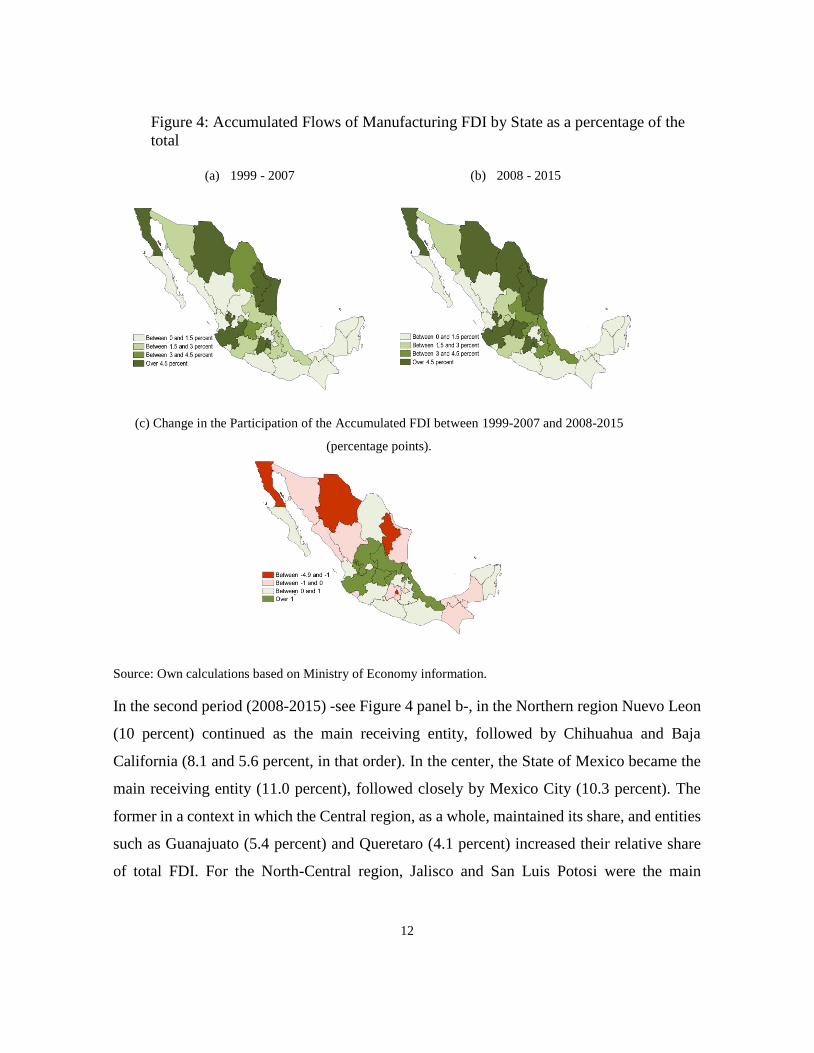
Figure 4: Accumulated Flows of Manufacturing FDI by State as a percentage of the

total

(a) 1999 - 2007 (b) 2008 - 2015

(c) Change in the Participation of the Accumulated FDI between 1999-2007 and 2008-2015

(percentage points).

Source: Own calculations based on Ministry of Economy information.

In the second period (2008-2015) -see Figure 4 panel b-, in the Northern region Nuevo Leon

(10 percent) continued as the main receiving entity, followed by Chihuahua and Baja

California (8.1 and 5.6 percent, in that order). In the center, the State of Mexico became the

main receiving entity (11.0 percent), followed closely by Mexico City (10.3 percent). The

former in a context in which the Central region, as a whole, maintained its share, and entities

such as Guanajuato (5.4 percent) and Queretaro (4.1 percent) increased their relative share

of total FDI. For the North-Central region, Jalisco and San Luis Potosi were the main

13

receiving entities (7.6 and 3.5 percent, respectively). In the South, Veracruz (4.4 percent)

continued as the principal recipient of manufacturing FDI in that region.

Figure 4 panel c shows the change in the participation of the entities, in percentage points

(p.p.), on the accumulated flows of manufacturing FDI between the two sub-periods

considered. The entities that appear in green are the ones that registered a positive variation,

whereas those that appear in red registered negative variations. As mentioned, some entities

located in the Central regions increased their participation during the period considered, in

particular, Guanajuato and Queretaro in the Central (1.9 p.p. each), and Jalisco, Zacatecas

(1.6 p.p. each) and San Luis Potosi (1.5 p.p.) in the North-Central.

In contrast, in the Northern region, only Coahuila increased its participation (0.7 p.p.), while

in the Southern region Veracruz presented the greatest positive variation (2.8 p.p.). Thus,

given the global crisis and its consequences on the external demand, the location of foreign

investment in manufacturing sector seems to be, in part, directing more towards the Central

regions, which are relatively more linked to the domestic market. It is important to mention

that part of this behavior also reflects the fact that a significant fraction of this investment has

been directed to the automotive sector, being located mainly in the Central regions.7

4 Model

In order to estimate the impact of states’ characteristics over the FDI flows during the period

1999-2015, we use a panel data approximation. We started with a standard fixed effects panel

estimation in order to take into account unobserved states’ individual characteristics (𝛼𝑖) that

can potentially bias our results.

ln(𝐹𝐷𝐼𝑖,𝑡) = 𝛼𝑖 + 𝛽𝑋𝑖,𝑡 + 𝜀𝑖,𝑡 (1)

7 As Sturgeon and Van Biesebroeck (2010) pointed out, the 2008-2009 global crisis accelerated pre-crisis

trends towards a greater importance of the automotive industry in developing and emerging economies.

14

𝜀𝑖,𝑡 ∼ 𝑁(0, 𝜎2𝐼𝑛)

Where ln(𝐹𝐷𝐼𝑖,𝑡) are the flows of Manufacturing Foreign Direct Investment across states 𝑖

in millions of constant 2008 pesos at year 𝑡.8

𝑋𝑖,𝑡is a matrix of control variables, that takes into account cost-oriented variables and

performance-oriented variables like:

• Total GDP, as a measurement of the size of the host market. This variable was

measured in constant millions of pesos (2008 base) excluding oil-related activities and

in natural logarithms.

• Average years of schooling among the population of 15 years or older as a

measurement of human capital, in logs.

• As a measure of agglomeration economies, we use the ratio of formal workers in the

manufacturing sector with respect to the total.

• Fiscal margin, measured as a percentage of unconditioned revenues (federal transfers

“participaciones” and own revenue, such as taxes and rights). This is a measurement

of the budget capacity of the state in order to give fiscal preferences to potential future

investments. It is expected that a state with less fiscal capacity cannot distract revenue

to attract new investments via fiscal incentives.9

• Crime, measured as intentional homicides per 10,000 inhabitants, in logs.

8 The data from the Ministry of Economy (Secretaría de Economía) are expressed in millions of current

dollars. For the conversion, we use the nominal peso/dollar exchange rate (fix), and the GDP deflator (2008

base) to convert the data in millions of constant pesos. We also considered this variable in millions of

constant dollars; however this did not change the results obtained below. 9 In Mexico, states’ public finances are highly dependent on federal transfers (Hernandez-Trillo and Jarillo-

Rabling, 2008). According to INEGI, on average, the sources of own revenue across federal entities

account for only 10 percent of the total.

15

• Infrastructure, measured by the telephone density for every 100 inhabitants, in logs.

• Wages, measured as the deviation of the daily wage reported to the social security in

pesos (real terms) of each state relative to the national average.10

• Real exchange rate, Mexican pesos per dollar, in order to capture external time shocks

that are common to all states, in logs.

Moreover, except for crime and wages, we expect a positive impact of these variables on

FDI, the dependent variable. Regarding the source of the variables, INEGI is the source of

most of them (the Mexican official statistics agency, in its publication “Statistical and

Geographical Yearbook by State”, Anuario Estadístico y Geográfico por Entidad

Federativa). Only fiscal margin and wages were obtained from the Mexican Ministry of

Finance (Secretaría de Hacienda y Crédito Público) and Ministry of Labor (Secretaría del

Trabajo y Previsión Social), both at State level.

To take into account the Market Potential variable (i.e. the size of the market in neighbor

states, measured as the spatially lagged log of the gross domestic product, see Blonigen et al.

2007) we estimate a Spatial Externalities Model (SLX):

𝑙𝑛(𝐹𝐷𝐼𝑖,𝑡) = 𝛼𝑖 + 𝛽𝑋𝑖,𝑡 + 𝜃𝑊𝑙𝑛(𝐺𝐷𝑃𝑖,𝑡) + 𝜀𝑖,𝑡 (2)

𝜀𝑖,𝑡 ∼ 𝑁(0, 𝜎2𝐼𝑛)

Also, to capture the potential spillover effect of FDI on neighbors, we include a Spatial

Durbin Model (SDM) into the analysis. This model takes into account the spatially lagged

dependent variable 𝑊𝑙𝑛(𝐹𝐷𝐼𝑖,𝑡) 11 and the spatially lagged GDP (Market Potential) and is

10 The wage for the manufacturing sector exclusively at the state level only was not available. Furthermore,

table A.1 in the appendix shows the descriptive statistics of the variables. 11 The matrix W quantifies the spatial connection between regions. In the present case, under the “queen

contiguity” principle, that is, one entity is considered to be neighboring to another only if they share a

common border. The matrix is binary and takes the value of 1 if the entities share border and zero

otherwise. Additionally, the elements of the main diagonal of W are equal to zero per construction. For

16

estimated by Maximum Likelihood (ML) and Generalized Method of Moments (GMM).

Failing to include the spillover effect of FDI, and/or the Market Potential12 into the analysis

may lead to biased and inefficient estimates (LeSage and Pace, 2009).

𝑙𝑛(𝐹𝐷𝐼𝑖,𝑡) = 𝛼𝑖 + 𝜌𝑊𝑙𝑛(𝐹𝐷𝐼𝑖,𝑡) + 𝛽𝑋𝑖,𝑡 + 𝜃𝑊𝑙𝑛(𝐺𝐷𝑃𝑖,𝑡) + 𝜀𝑖,𝑡 (3)

𝜀𝑖,𝑡 ∼ 𝑁(0, 𝜎2𝐼𝑛)

Hence, the SDM allows us to:

1. Estimate if FDI allocation decisions may result in a reduced participation in neighbor

states, leading to a "race to the bottom" among states in order to secure the investment,

or in a spill-over effect across states that can lead to an increase in FDI in neighbor

states.

2. Decompose the impact of the characteristics of interest regarding direct impacts on the

states or those characteristics of the neighbors (indirect effects), see below.

Since the interpretation of the parameters’ estimates are different from non-spatial regression

techniques and using the correct measurements is not usual in the literature of FDI, we will

put emphasis on the estimations of direct and indirect effects.

According to LeSage and Pace (2009), interpreting the coefficients of the independent

variables from a spatial regression, specifically Spatial Auto-regressive Model and Spatial

Durbin Model, is not straightforward. In the case of OLS and non-related observations, the

derivative from 𝑦𝑖 with respect to 𝑥𝑖𝑘 is:

more details, definitions and interpretations of the spatial econometric models employed, see the sections

A.3 to A.5 of the appendix. 12 Given that it is, somehow, correlated with another independent variable.

17

𝜕𝑦𝑖𝜕𝑥𝑖𝑘

= 𝛽𝑘 (4)

In the case of Spatial Durbin Model, the 𝛽𝑘 coefficients cannot be interpreted in the same

fashion given that:

𝜕𝑦𝑖𝜕𝑥𝑖𝑘

= (𝐼𝑛 − 𝜌𝑊)−1(𝛽𝑘 +𝑊𝜃𝑘) (5)

Where θ is the coefficient for the spatial lag of the independent variable 𝑋𝑘, and ρ is the

coefficient for the spatial lag of the dependent variable for the Spatial Auto-regressive Model,

the coefficient is:

𝜕𝑦𝑖𝜕𝑥𝑖𝑘

= (𝐼𝑛 − 𝜌𝑊)−1(𝛽𝑘) (6)

And it is the presence of (𝐼𝑛 − 𝜌𝑊)−1that makes the cross derivatives among observations

different from zero. In other words, unlike non-spatial models (and the SEM), the derivative

of 𝑦𝑖 with respect to 𝑥𝑗𝑘 may be potentially not zero. This allows the existence of spillovers

effects since a small change in the observation 𝑗 can affect the dependent variable in region

𝑖 (LeSage and Pace, 2009).

In order to isolate these two effects (the impacts on the dependent variable for observation 𝑖

given changes in 𝑋𝑖𝑘 -direct, and the impacts on the dependent variable for observation 𝑖

given changes in 𝑋𝑗𝑘, -indirect), we used the impact calculations of Piras (2013) based on

Kelejian et al. (2006) and LeSage and Pace (2009).

Furthermore, W is a panel, row-standardized contiguity neighbor weight matrix, ρ is the

spatial auto-regressive coefficient that measures the spatial relationship of FDI of neighbor

states.

According to Regelink and Elhorst (2015) and the definitions provided by Escobar (2013) if

𝜌 = 0 and 𝜃ln(𝐺𝐷𝑃) = 0 we are in the presence of horizontal FDI, and the estimation of an

18

a-spatial model will be enough to obtain unbiased and efficient estimators. Escobar (2013)

describes it as a “pure horizontal FDI” where “a parent firm decides to open a filial to supply

the local market”, in this case FDI only follows its determinants for each of the regions

independently and it is competitive among states, i.e. more FDI in state 𝑖 means less for state

𝑗. If 𝜌 < 0 and 𝜃ln(𝐺𝐷𝑃) = 0 is the case of vertical FDI, where an investing foreign firm

outsources part of its production to lower costs, in this case, we face a competitive FDI among

regions in order to obtain access to low-cost inputs. 𝜌 < 0 and 𝜃ln(𝐺𝐷𝑃) > 0 is export-

platform FDI, where a investing foreign firm invest in the region to supply a third region and

𝜌 > 0 and 𝜃ln(𝐺𝐷𝑃) ≥ 0 is complex vertical FDI, where a firm spreads its production chain

among several neighbouring regions in order to access cost-differential inputs.

Finally, the Durbin Spatial Model of the equation (3) is estimated by both Generalized

Method of Moments (GMM) and Maximum Likelihood (ML) taking into account the

nonlinearity of the equation13. The reason to employ ML in addition to GMM is that, to the

best of our knowledge, decomposition between direct and indirect effects is not availaible for

the GMM estimator. However, as we shall see below both methods of estimation yield very

similar results.

5 Results

In table 1 we show the estimation results of Equation 1-3, the first column corresponds with

the a-spatial fixed effects with robust standard errors, an SLX model (in order to include a

local spillover effect of the Market Potential) and a Spatial Durbin Model (SDM) with direct

and indirect effects.

13 Folowing Anselin (1988), since we have a dependent variable in the right hand part of the equation, re-

expressing the model 𝑦 = 𝜌𝑊𝑦 + 𝑋𝛽 + 𝜀, as 𝐴𝑦 = 𝑋𝛽 + 𝜀, with 𝐴 = 𝐼 − 𝜌𝑊, and the error term

would be expressed as 𝜀 = Ω1

2𝑣 give us Ω1

2(𝐴𝑦 − 𝑋𝛽) = 𝑣, or 𝑓(𝑦, 𝑋, 𝜃) = 𝑣, with 𝜃 as a vector of

parameters, and f is not linear in y, X and 𝜃

19

Table 1: Estimation Results, A-Spatial Fixed Effects, SLX and Durbin Model. Dependent

Variable: Log of Manufacturing FDI in 2008 Constant Pesos

Variable

(Eq.1) (Eq.2) (Eq. 3), Panel SDM (Eq.3), Panel SDM

Coefficient Estimates Marginal Effects (ML)

Fixed Panel ML GMM Direct Indirect

Effects SLX FE FE Effects Effects

𝜌 0.376*** 0.435***

(8.02) (2.38)

𝑙𝑛(𝐺𝐷𝑃)1 -0.252 -0.180 -0.206 -0.210 -0.256 -1.089

(-0.34) (-0.21) (-0.26) (-0.27) (-0.34) (-0.73)

Wages -0.012* -0.012* -0.010* -0.010 -0.011* -0.006

(-1.72) (-1.67) (-1.63) (-1.59) (-1.72) (-1.61)

ln(Education) 5.775*** 6.033** 5.804*** 5.768*** 5.941* 3.268*

(3.17) (2.61) (2.72) (2.68) (2.70) (2.41)

ln(Telephone

density)

0.556 0.551 0.535 0.532 0.548 0.303

(1.56) (1.54) (1.62) (1.60) (-1.59) (1.49)

Agglomeration 9.433*** 9.395*** 7.724*** 7.462*** 7.933*** 4.366***

(4.20) (4.16) (3.68) (3.32) (3.62) (2.94)

Fiscal Margin 1.879* 1.930* 1.991** 2.001** 2.092** 1.149**

(1.86) (1.84) (2.05) (2.05) (2.08) (1.95)

ln(Homicides) -0.093 -0.090 -0.024 -0.014 -0.021 -0.012

(-0.76) (-0.73) (-0.21) (-0.12) (-0.18) (-0.18)

ln(Real

Exchange Rate)

-1.056 -1.052 -0.700 -0.645 -0.717 -0.393

(-1.17) (-1.17) (-0.84) (-0.76) (-0.83) (-0.81)

Market Potential -0.207 -0.684 -0.758 See:

(-0.18) (-0.64) (-0.70) 𝑙𝑛(𝐺𝐷𝑃)1

𝑅2 0.063 0.064 0.729 0.734 N/A

Log likelihood N/A N/A -1720.1 N/A N/A

N 544 544 544 544 544

T 17 17 17 17 17

(1) GDP does not include oil-related activities; Spatial Matrix defined as "Queen" contiguity.

t-values in parenthesis; *** p<0.01, ** p<0.05, * p<0.1.

Lee-Yu corrected standard errors for ML models; for the estimation of the Durbin model, we used Millo and

Piras (2012) splm package in R. The last two columns reports the marginal effects coefficients.

20

We used fixed effects in all specifications given the nature of the data (units are not randomly

selected from a population). The first column shows the effects of the determinants using a

spatially blind model, with a positive and statistically significant impact of education,

infrastructure, agglomeration, fiscal margin, and negative impacts of wages. GDP

(measurement of the size of the state’s economy) shows a negative one, but is not statistically

different from zero.

With these results, we can infer that manufacturing FDI is attracted to states with higher

educated population, larger telecommunication infrastructure, and with a higher ratio of

workers employed in the manufacturing sector. Also, it is negatively related to salaries. In

this particular variable, the average of the daily wage in the formal sector in Mexico is 294.00

pesos (around 15 dollars per day), since the variable in the model is measured as a deviation

from the national average, it means that an increase of one peso with respect to the nation

average represents a reduction of 0.01% in FDI.

When we include the market potential (equation 2, SLX model) is not significat at 10%,

meaning that FDI does not get attracted to internal markets (export-oriented industries). By

contrast, the fiscal margin (the budget capacity of a state’s government) is positive and

statistically significant, meaning that states with higher budget independence (those that do

not rely completely on federal transfers) get a higher FDI. This budget independence provides

each local government with a better condition to bargain with potential investors, for

example.

So far, with the exception of the new result of our variable about fiscal incentives, the results

are in line with the evidence obtained from the four studies indicated in section 2.2 in the

case of Mexico for variables human capital, crime/delinquency, wages, and agglomeration.

In the case of infrastructure, our results differ from those obtained by Jordaan (2008, 2012)

regarding his estimations for the manufacturing sector. In the case of the spatial study of

Escobar (2013), the sign of the variable is sensitive to the inclusion of fixed effects. In our

case, as we shall see through the decomposition of the effects, this variable has a positive

impact, both direct and indirect. Furthermore, the novel result concerning the fiscal margin

21

is only significant at 10% on the SLX specification. However, its impact becomes clearer

when we consider the Durbin specification in the following columns.

With the spillover effects estimation (equation 3, SDM model), we reported direct and

indirect effects of each variable and the spatial spillover coefficient ρ. It follows a similar

direct effect compared with the a-spatial fixed effects model with a highly significant positive

spillover effect between 0.36 (ML) and 0.43 (GMM), meaning that an increase of 10% in the

average FDI flows in the neighbors of the state i will increase the FDI in that state, on average,

between 3.6% - 4.3%. This result, the positive spatial spillover effect (not its magnitude), is

similar to Escobar (2013) in the Mexican case, although his estimations were carried out with

a spatial autoregressive (SAR) model with no decomposition effects and for total FDI,

measured as a stock as we previously mentioned in the literature review.

With the indirect decomposition, we can measure the spillover effect for each of the

determinants of FDI, with a positive spillover effect on education, agglomeration and fiscal

margin; meaning that improving those conditions will benefit neighbors’ capacity to attract

FDI, and telecommunication infrastructure with positive direct impact only, meaning that a

improving of this variable by state A will enhance only that state capacity to atrract FDI and

none of their neigbours’. Moreover, the market potential remains negative although not

significant. 14 This latter result, along with the positive spatial spillover effect referred

previously, imply that manufacturing FDI across Mexican states corresponds to the complex

vertical case (Regelink and Elhorst, op. cit.).

One clear example of this refers to the investments in the automobile sector, which account

for one-quarter of total FDI in manufacturing between 1999-2015 (see figure 1): with the

arrival of new assembly plants, suppliers locate close to these places (in the same state or in

14 We consider a lag on GDP to control for endogeneity issues, but results were not different. Additionally,

we perform the Granger causality test for panel data developed by Abrigo and Love (2015). The results

are in table A.2 of the appendix and show that, for variables susceptible to presenting this problem such as

GDP, agglomeration, schooling and telephone density, the causality runs from the aforementioned

variables to the manufacturing FDI flows and not vice versa. In the case of wages, there was no causation.

22

neighboring ones)15 spreading its productions chains looking for benefits in cost factor

access. Likewise, given that roughly 80% of cars produced are destined to foreign markets

(Secretaría de Economía, 2016), it is obviously the relevant market for this industry (like

electric equipment and electronic components), not the local or regional market.

The Foreign Direct Investment shows a positive spillover effect on average across Mexican

states, implying a positive synergy of the investment in neighbor states. A potential cluster

behavior may be happening (foreign manufacturing investment tends to concentrate around

the same region, hence sharing resources and lowering costs). Also, the fiscal margin is a key

factor to attract investment, maybe lowering cost with lower local taxes and land-granting

programs.

Human Capital shows a positive relationship, direct and indirect, meaning that increasing the

level of education not just raises foreign investment in that particular state but also in nearby

regions. Specialization has a positive direct impact (a large pool of specialized workers is

positively related to higher foreign investment) and has positive spillover effects among

states’ neighbors. Finally, the homicides variable has the expected sign but is not statistically

significant on any of the different specifications.

On the other hand, the decision of neighborhood was arbitrary, since we selected a contiguity

definition for W (i.e. states with common border are neighbors), there is a criticism that the

results may be driven by a different definition of W.16

We tested a different neighbor matrix based on three nearest neighbors (see figure A.1 in the

appendix) instead of using border contiguity, and re-estimated equation 2 and 3. The results

are presented in table 2. The results are practically in the same direction and statistically

15 For example, according to INEGI two of the states with the most weight of the production of automobile

sector in the country, Coahuila and Guanajuato, increased by 52.3% and 102.4% the number of economic

units dedicated to produce auto parts between 2008 and 2013, respectively (from 88 to 124 and from 42 to

84, in that order). 16 Although LeSage and Pace (2014) suggest that this criticism is misleading, since any W will capture the

immediate and more important neighbor impacts.

23

significant, with a stronger spillover effect (0.44 vs. 0.38) and an wages with a significance

of 10% in direct impact, meaning that the spatial effect is strong enough to be captured by

the two different selections of W.

Table 2: Estimation Results with Alternative W (3 nearest neighbors), SLX and Durbin

Model. Dependent Variable: Log of Manufacturing FDI in 2008 Constant Pesos

Variable

(Eq.2) (Eq. 3), Panel SDM

Coefficient Estimates Marginal Effects (ML)

Panel ML GMM Direct Indirect

SLX FE FE Effects Effects

𝜌 0.376*** 0.435**

(8.02) (2.38)

ln(𝐺𝐷𝑃)1 -0.252 -0.206 -0.210 -0.317 -1.171

(-0.34) (-0.26) (-0.27) (-0.41) (-0.80)

Wages -0.012* -0.010* -0.010 -0.011 -0.006

(-1.72) (-1.63) (-1.59) (-1.62) (-1.52)

ln(Education) 5.775*** 5.804** 5.768** 6.071*** 3.346**

(3.17) (2.72) (2.68) (2.67) (2.39)

ln(Telephone Density) 0.556 0.535 0.532 0.538 0.295

(1.56) (1.62) (1.60) (1.52) (1.45)

Agglomeration 9.433*** 7.724*** 7.462*** 7.904*** 4.349***

(4.20) (3.68) (3.32) (3.68) (3.06)

Fiscal Margin 1.879* 1.991** 2.001** 2.051** 1.131*

(1.86) (2.05) (2.05) (2.04) (1.89)

ln(Homicides) -0.093 -0.024 -0.014 -0.026 -0.015

(-0.76) (-0.21) (-0.12) (-0.22) (-0.23)

ln(Real Exchange

Rate)

-1.056 -0.700 -0.645 -0.708 -0.388

(-0.52) (-0.84) (-0.76) (-0.83) (-0.80)

Market Potential -0.098 -0.684 -0.758 See:

(-0.08) (-0.64) (-0.70) 𝑙𝑛(𝐺𝐷𝑃)1

𝑅2 0.063 0.729 0.734 N/A

Log likelihood N/A -1720.1 N/A N/A

N 544 544 544 544

T 17 17 17 17

(1) GDP does not include oil-related activities.

t-values in parenthesis. *** p<0.01, ** p<0.05, * p<0.1 .

Lee-Yu corrected standard errors; for the estimation of the Durbin model, we used Millo and Piras (2012) splm

package in R. The last two columns reports the marginal effects coefficients.

24

6 Conclusions

The results of this study show that FDI has complementarity effects, that is, if the FDI

amounts attracted by neighboring entities increase, then the investment amounts captured by

the reference entity also tend to go up. Thus, in addition to direct and indirect impacts of the

variables such as schooling, agglomeration, and infrastructure on FDI, this suggests the

presence of positive externalities in the processes of attracting FDI from the manufacturing

sector. Moreover, these results along with those novel findings regarding fiscal margin

variable (both direct and indirect), support the argument. Regarding public policies aimed at

increasing flows of this type of investment, estimates suggest that, because of the positive

pattern of spatial dependence in the FDI localization process, the attraction of FDI should be

considered in a regional context and not only from a local perspective.

Further research might distinguish between "new" and "total" FDI since total flows of FDI

include re-investments of existing foreign capital and firms. Also, it must include other

sectors into the analysis (e.g. export-oriented manufacturing) as well as the total flows of

investments.

Finally, in the case of the Southern region, which captures the smallest amounts of

manufacturing FDI, it is relevant to consider the potential impact of the reform on the

implementation of the Special Economic Zones (SEZ) as a factor that may enhance the

attractiveness of this region. Cheng and Kwan (2000) show that this is the case for the

Chinese regions that have SEZ,17 hence the relevance of the correct implementation of this

initiative as a factor that can boost the dynamism of the economy of this region.

17 For further evidence see Lim (2001).

25

7 References

Abrigo, M. R., and Love, I. (2015). Estimation of panel vector autoregression in Stata: A

package of programs. manuscript, Febr 2015 available on http://paneldataconference2015.

ceu. hu/Program/Michael-Abrigo. pdf.

Blonigen, B. A., Davies, R. B., Waddell, G. R., and Naughton, H. T. (2007). FDI in space:

Spatial autoregressive relationships in foreign direct investment. European Economic

Review, 51(5), 1303-1325.

Bobonis, G. J., and Shatz, H. J. (2007). Agglomeration, adjustment, and state policies in the

location of foreign direct investment in the United States. The Review of Economics and

Statistics, 89(1), 30-43.

Borensztein, E., De Gregorio, J., and Lee, J. W. (1998). How does foreign direct investment

affect economic growth?. Journal of international Economics, 45(1), 115-135.

Casi, L., and Resmini, L. (2014). Spatial complexity and interactions in the FDI attractiveness

of regions. Papers in Regional Science, 93(S1), S51-S78.

Cheng, L. K., and Kwan, Y. K. (2000). What are the determinants of the location of foreign

direct investment? The Chinese experience. Journal of International Economics, 51(2), 379-

400.

Coughlin, C. C., and Segev, E. (2000). Foreign direct investment in China: a spatial

econometric study. The World Economy, 23(1), 1-23.

Coughlin, C. C., Terza, J. V., and Arromdee, V. (1991). State characteristics and the location

of foreign direct investment within the United States. The Review of economics and

Statistics, 675-683.

Crozet, M., Mayer, T., and Mucchielli, J. L. (2004). How do firms agglomerate? A study of

FDI in France. Regional Science and Urban Economics, 34(1), 27-54.

Deichmann, J., Karidis, S., and Sayek, S. (2003). Foreign direct investment in Turkey:

regional determinants. Applied Economics, 35(16), 1767-1778.

26

Durham, J. B. (2004). Absorptive capacity and the effects of foreign direct investment and

equity foreign portfolio investment on economic growth. European economic review, 48(2),

285-306.

Escobar Gamboa, O. R. (2013). Foreign direct investment (FDI) determinants and spatial

spillovers across Mexico's states. The Journal of International Trade and Economic

Development, 22(7), 993-1012.

Elhorst, J. P. (2014). Spatial econometrics: from cross-sectional data to spatial panels (pp.

20-25). Berlin: Springer.

Glaeser, E. L. (Ed.). (2010). Agglomeration economics. University of Chicago Press.

Hanson, G. H. (1996). Agglomeration, dispersion, and the pioneer firm. Journal of Urban

Economics, 39(3), 255-281.

Hernandez-Trillo, F., and Jarillo-Rabling, B. (2008). Is local beautiful? Fiscal

decentralization in Mexico. World Development, 36(9), 1547-1558.

Hill, S., and Munday, M. (1992). The UK regional distribution of foreign direct investment:

analysis and determinants. Regional Studies, 26(6), 535-544.

Jones, J., and Wren, C. (2016). Does service FDI locate differently to manufacturing FDI? A

regional analysis for Great Britain. Regional Studies, 50(12), 1980-1994.

Jordaan, J. A. (2008). State characteristics and the locational choice of foreign direct

investment: Evidence from regional FDI in Mexico 1989–2006. Growth and Change, 39(3),

389-413.

Jordaan, J. A. (2012). Agglomeration and the location choice of foreign direct investment:

new evidence from manufacturing FDI in Mexico. Estudios Económicos, 61-97.

Kelejian, H. H., Tavlas, G. S., and Hondroyiannis, G. (2006). A spatial modelling approach

to contagion among emerging economies. Open economies review, 17(4), 423-441.

27

Ledyaeva, S. (2009). Spatial econometric analysis of foreign direct investment determinants

in Russian regions. The World Economy, 32(4), 643-666.

Lee, L. F. (2004). Asymptotic Distributions of Quasi‐Maximum Likelihood Estimators for

Spatial Autoregressive Models. Econometrica, 72(6), 1899-1925.

Lee, K. D., and Hwang, S. J. (2014). Regional heterogeneity and location choice of FDI in

Korea via agglomeration and linkage relationships. Journal of the Asia Pacific

Economy, 19(3), 464-487.

LeSage, J. P., and Pace, R. K. (2009). Introduction to Spatial Econometrics (Statistics,

textbooks and monographs). CRC Press.

LeSage, J. P., and Pace, R. K. (2014). The biggest myth in spatial

econometrics. Econometrics, 2(4), 217-249.

Li, X., and Liu, X. (2005). Foreign direct investment and economic growth: an increasingly

endogenous relationship. World Development, 33(3), 393-407.

Lim, E. G. (2001). Determinants of, and the Relation Between FDI and Growth: A Summary

of the Recent Literaturre. WP n 01/75, IMF.

Millo, G., and Piras, G. (2012). splm: Spatial panel data models in R. Journal of Statistical

Software, 47(1), 1-38.

Mollick, A. V., Ramos-Duran, R., and Silva-Ochoa, E. (2006). Infrastructure and FDI

inflows into Mexico: a panel data approach. Global Economy Journal, 6(1), 1-25.

Mukim, M., and Nunnenkamp, P. (2012). The location choices of foreign investors: A

district‐level analysis in India. The world economy, 35(7), 886-918.

Piras, Gianfranco, “Impact Estimates for Static Spatial Panel Data Models in R," Mimeo,

2013.

28

Porter, M. (2003). “The Economic Performance of Regions”. Regional Studies, Vol. 37, pp.

549-578.

Regelink, M., and Elhorst, J. P. (2015). The spatial econometrics of FDI and third country

effects. Letters in Spatial and Resource Sciences, 8(1), 1-13.

Schäffler, J., Hecht, V., and Moritz, M. (2016). Regional determinants of German FDI in the

Czech Republic: new evidence on the role of border regions. Regional Studies, 1-13.

Sturgeon, Timothy and Johannes Van Biesebroeck, (2010) “Effects of the crisis on the

automotive industry in developing countries: a global value chain perspective," Policy

Research Working Paper 5330.

29

Appendix

Figure A.1: Two definitions of W: 3 nearest neighbors (above), Queen-contiguity

neighbors (below).

Souce: Own elaboration with information from INEGI.

30

Table A.1 Descriptive Statistics

Souce: Own calculations with information from INEGI and Ministry of Economy.

Mean Standard Deviation Min Max

ln (FDI) 7.20 1.90 1.31 10.76

ln (GDP) 12.32 0.80 10.84 14.65

Wages 0.00 33.82 -57.99 118.29

ln (Education) 2.10 0.12 1.68 2.39

ln (Telephone density) 2.59 0.46 1.09 4.16

Agglomeration 0.25 0.15 0.02 0.69

Fiscal Margin 0.42 0.10 0.21 1.00

ln (Homicides) -0.96 0.99 -3.08 1.73

Total number of observations

Number of cross sections

Time periods

544

32

17

Variable

31

Table A.2 Panel Granger Causality Test

Note: ⇏ denotes “non causality”; *** p<0.01, ** p<0.05

Souce: Own calculations with information from INEGI and Ministry of Economy.

Causality Relation Lags Chi Square

8.23 0.00 ***

0.00 0.98

10.92 0.00 ***

1.89 0.38

5.18 0.02 **

0.23 0.62

0.19 0.90

0.28 0.86

7.01 0.00 ***

2.59 0.10

0.14 0.92

0.99 0.60

8.15 0.00 ***

0.05 0.81

11.71 0.00 ***

3.87 0.14

0.28 0.59

0.00 0.96

0.30 0.85

0.03 0.982

1

2

1

2

1

p-value

1

2

1

2

ln (𝐹𝐷𝐼) ⇏ ln (𝐺𝐷𝑃)

ln (𝐺𝐷𝑃) ⇏ ln (𝐹𝐷𝐼)

ln (𝐹𝐷𝐼) ⇏ ln (𝐺𝐷𝑃)

ln (𝐺𝐷𝑃) ⇏ ln (𝐹𝐷𝐼)

ln (𝐹𝐷𝐼) ⇏ l n

l n ⇏ ln (𝐹𝐷𝐼)

ln (𝐹𝐷𝐼) ⇏ l n

l n ⇏ ln (𝐹𝐷𝐼)

ln 𝐹𝐷𝐼 ⇏ ln (𝑡 𝑙 𝑛 𝑛 𝑖𝑡𝑦)

ln 𝑡 𝑙 𝑛 𝑛 𝑖𝑡𝑦 ⇏ ln (𝐹𝐷𝐼)

ln 𝐹𝐷𝐼 ⇏ ln (𝑡 𝑙 𝑛 𝑛 𝑖𝑡𝑦)

ln 𝑡 𝑙 𝑛 𝑛 𝑖𝑡𝑦 ⇏ ln (𝐹𝐷𝐼)

ln 𝐹𝐷𝐼 ⇏ ln ( 𝑙𝑖𝑛 )

ln 𝑙𝑖𝑛 ⇏ ln (𝐹𝐷𝐼)

ln 𝐹𝐷𝐼 ⇏ ln ( 𝑙𝑖𝑛 )

ln 𝑙𝑖𝑛 ⇏ ln (𝐹𝐷𝐼)

ln 𝐹𝐷𝐼 ⇏ ln ( )

ln ⇏ ln (𝐹𝐷𝐼)

ln 𝐹𝐷𝐼 ⇏ ln ( )

ln ⇏ ln (𝐹𝐷𝐼)

32

A.3 Constructing a Neighbor Matrix (W)

In the following sections, since we are going to discuss the effects on one region dependent

variable with the values of neighbor regions it is important to formalize the construction of

the Neighbor Matrix (W).

Assume this geographical distribution of Y among 8 regions:

𝑦1 𝑦2 𝑦3 𝑦4

𝑦5 𝑦6 𝑦7 𝑦8

Moreover, suppose the economic relationship is higher with neighbors, defined as those with

a common border in a Rook (as in chess) relationship. For example, region 6 will have three

neighbors: region 2, 5 and 7, depicted in the following diagram:

𝑦2

𝑦5 𝑦6 𝑦7

Moreover, we can represent all the relationships in a squared Matrix (here named 𝑊1) with a

number of columns and rows equal to the number of regions, where one means neighbor

relationship and zero otherwise. For example, region 6 (highlighted) shows neighbor

relationship with region 2, 5 and 7 (column 2, 5 and 7 respectively). The main diagonal

should always have zero value since a region is not a neighbor of itself.

𝑊1 =

(

0 1 0 0 1 0 0 01 0 1 0 0 1 0 00 1 0 1 0 0 1 00 0 1 0 0 0 0 11 0 0 0 0 1 0 00 1 0 0 1 0 1 00 0 1 0 0 1 0 10 0 0 1 0 0 1 0)

33

This matrix must be row-normalized, in order to capture the average effect of neighbor

regions,

𝑊2 =

(

0 1/2 0 0 1/2 0 0 01/3 0 1/3 0 0 1/3 0 00 1/3 0 1/3 0 0 1/3 00 0 1/2 0 0 0 0 1/21/2 0 0 0 0 1/2 0 00 1/3 0 0 1/3 0 1/3 00 0 1/3 0 0 1/3 0 1/30 0 0 1/2 0 0 1/2 0 )

Assume we have the following values for each region: 𝑋𝑇 = (3, 8, 6, 4, 9, 1, 2, 5), so 𝑊2𝑋

is equal to the mean of the neighbors for each region, this “new” variable is called “X spatially

lagged”.

A.4 Spatial Econometrics Explanation

It is well known that investments in one state impacts beyond administrative borders into

nearby cities and towns. Following Elhorst (2014), we start with “a more general model

containing a series of simpler models that ideally should represent all the alternative

economic hypotheses…” Since there are three different types of interactions possible, we

will concentrate our efforts in two interactions that are relevant to our case:

First case: Dependent variable of region i is determined in part by the value of the dependent

variable of neighbor region j.

This can be expressed as: 𝑦 = 𝜌𝑊𝑦 + 𝛼 + 𝑋𝛽 + 𝜀 , where 𝑊𝑦 is the average of the

dependent variable (see previous section) of the neighbors for each i (i.e. ∑ 𝑖𝑗𝑁𝑗≠𝑖 𝑦𝑖 for each

i ). This is known in the spatial econometrics literature as the Spatial Autoregressive

Regression (SAR).

In this case, we need to solve 𝑦 = (𝐼𝑛 − 𝜌𝑊)−1(𝑋𝛽 + 𝛼 + 𝜀), with 𝜀 ∼ 𝑁(0, 𝜎2𝐼𝑛)

34

Second case: Dependent variable of region i is determined in part by the value of an

independent variable of neighbor region j.

This can be expressed as: 𝑦 = 𝛼 + 𝑋𝛽 +𝑊𝑋𝜃 + 𝜀, where 𝑊𝑋 is the average of (some)

independent variables of the neighbors for each i. This is known in the spatial econometrics

literature as the Spatial Lag of X model (SLX).

Also, there is a combination of the two cases: 𝑦 = 𝜌𝑊𝑦 + 𝛼 + 𝑋𝛽 +𝑊𝑋𝜃 + 𝜀 and is

known as the Spatial Durbin Model (SDM).

In this case, we need to solve 𝑦 = (𝐼𝑛 − 𝜌𝑊)−1(𝑋𝛽 +𝑊𝑋𝜃 + 𝛼 + 𝜀), with 𝜀 ∼ 𝑁(0, 𝜎2𝐼𝑛)

In order to estimate SAR and SDM models, we cannot use OLS since they lead to

“inconsistent estimates of the regression parameters for models with spatially lagged

dependent variables” (LeSage and Pace, 2009), so Maximum Likelihood is used instead (Lee,

2004). In contrast, SLX models can be estimated with OLS procedures.

A.5 Direct and Indirect Effects:

As is explained in the text (p.18), interpreting the parameter estimates (𝛽, 𝜃) is not

straightforward, since the right-hand part of the equation is pre-multiplied by (𝐼𝑛 − 𝜌𝑊)−1.

Equation 6 implies that “a change in the explanatory variable for a single region (observation)

can potentially affect the dependent variable in all other observations (regions)” (Lesage and

Pace, 2009).

In order to measure the impacts of a specific independent variable, we must separate the

impacts on the dependent variable of a specific region caused by changes in same region’s

independent variables (this includes potential feedback loops), and impacts caused by

changes in other region’s independent variables. Pace and LeSage (2006) suggest a

computational way to measure those impacts based on the following matrix (for all i and j)

35

𝜕𝑦𝑖

𝜕𝑥𝑗𝑟= (𝐼𝑛 − 𝜌𝑊)

−1(𝛽𝑟 +𝑊𝜃𝑟). Average Total Impacts to an Observation is the average of

row sums. The Average Direct Impact is the average of the diagonal of the matrix, and the

Indirect Impact is the difference between them.

From LeSage and Pace (2009), for each independent variable r:

Direct Effect (r) = 𝑛−1𝑡𝑟((𝐼𝑛 − 𝜌𝑊)−1(𝛽𝑟 +𝑊𝜃𝑟))

Total Effect (r) = 𝑛−1𝜄′𝑛(𝐼𝑛 − 𝜌𝑊)−1(𝛽𝑟 +𝑊𝜃𝑟)𝜄𝑛

Indirect Effect (r) = Total Effect (r) – Direct Effect (r)

Where tr is the trace and 𝜄′𝑛 is the a vector of ones of dimension n. The standard deviations

are created via Monte Carlo simulations; we use a modified version of splm package of Piras

in order to allow a panel Durbin model with only one dependent variable spatially lagged.