Determinants of Japanese Yen Interest Rate Swap Spreads: Evidence from a Smooth Transition Vector Autoregressive Model

Ying Huang Manhattan College

Carl R. Chen*

University of Dayton

Maximo Camacho Bank of Spain and University of Murcia

(Current version: January 2007)

Abstract ________________________________________________________________________ This paper investigates the determinants of variations in the yield spreads between Japanese yen interest rate swaps and Japan government bonds for a period from 1997 to 2005. A smooth transition vector autoregressive (STVAR) model and generalized impulse response functions are used to analyze the impact of various economic shocks on swap spreads. The volatility based on a GARCH model of the government bond rate is identified as the transition variable that controls the smooth transition from high volatility regime to low volatility regime. The break point of the regime shift occurs around the end of the Japanese banking crisis. The impact of economic shocks on swap spreads varies across the maturity of swap spreads as well as regimes. Overall, swap spreads are more responsive to the economic shocks in the high volatility regime. Moreover, volatility shock has profound effects on shorter maturity spreads, while the term structure shock plays an important role in impacting longer maturity spreads. Our results also show noticeable differences between the non-linear and linear impulse response functions. JEL classification: G15, E43 Keywords: Japanese yen interest rate swap, smooth transition VAR, regime switching. * Corresponding author: Carl R. Chen, Department of Economics and Finance, University of Dayton, 300 College Park, Dayton, Ohio 45469-2251. Tel: (937)229-2418, Fax: (937)229-2477, E-mail: chen@udayton.edu. We thank two anonymous reviewers and the editor, Bob Webb, for helpful comments. The views in this paper are those of the authors and do not represent the views of the Bank of Spain or the Eurosystem.

2

Determinants of Japanese Yen Interest Rate Swap Spreads: Evidence from a

Smooth Transition Vector Autoregressive Model Abstract ________________________________________________________________________ This paper investigates the determinants of variations in the yield spreads between

Japanese yen interest rate swaps and Japan government bonds for a period from 1997 to

2005. A smooth transition vector autoregressive (STVAR) model and generalized

impulse response functions are used to analyze the impact of various economic shocks on

swap spreads. The volatility based on a GARCH model of the government bond rate is

identified as the transition variable that controls the smooth transition from high volatility

regime to low volatility regime. The break point of the regime shift occurs around the end

of the Japanese banking crisis. The impact of economic shocks on swap spreads varies

across the maturity of swap spreads as well as regimes. Overall, swap spreads are more

responsive to the economic shocks in the high volatility regime. Moreover, volatility

shock has profound effects on shorter maturity spreads, while the term structure shock

plays an important role in impacting longer maturity spreads. Our results also show

noticeable differences between the non-linear and linear impulse response functions.

3

Determinants of Japanese Yen Interest Rate Swap Spreads: Evidence from a Smooth Transition Vector Autoregressive Model

1. Introduction

This paper provides an empirical examination of the dynamic behavior of the

Japanese yen interest rate swap spreads1 (hereafter swap spreads) and relevant risk factors

within a smooth transition vector autoregressive (STVAR) framework. The non-linear,

state-dependent model better characterizes the Japanese swap market since the late 1990s,

and it uncovers asymmetric and regime-shifting movements in swap spreads.

Being the price of interest rate swaps, swap spreads constitute an important

research topic as swap contracts have experienced exponential worldwide growth over

the past decade with the widespread use by corporations, hedge funds, and other financial

institutions for risk management. Increasingly municipal governments have also entered

interest rate swap agreements to manage their debt. In addition to the growing popularity

of interest rate swaps for risk management, financial market in the US increasingly has

adopted the swap curve for bonds and derivative securities pricing due to the dwindling

liquidity in the Treasury market.2 Among the major players, Japanese yen interest rate

swap plays a pivotal role in the global interest rate derivatives market. It amounts to an

average of 15% of the total outstanding interest rate derivatives worldwide. The

expansion in the Japanese yen interest rate swap speaks for the importance of

understanding the yen swap pricing mechanism. Surprisingly, few studies have

1 They are the spreads between Japanese yen interest rate swaps and Japanese government bonds with comparable maturities. 2 One-year T-bill was phased out in 2000, while the issuance of 30-year T-bonds was stopped in 2001.

4

undertaken the task of seeking an appropriate explanation of the Japanese swap market

dynamics.3

This research thus contributes to the literature in a number of aspects. First, we

study the behavior of Japanese swap spreads whose importance is second only to the US

counterpart, yet are much ignored and under-studied. Second, instead of using either a

static single equation regression analysis or a linear vector autoregressive (VAR) model

common in most swap studies, we employ a smooth transition vector autoregressive

(STVAR) model to examine the asymmetric effects of economic shocks on Japanese

swap spreads. The non-linear STVAR model allows for a smooth transition from one

regime of swap spreads to the other, controlled by an underlying economic determinant.

Third, our sample spans from 1997 to 2005, which not only offers the most

updated dataset, but also encompasses the Japanese banking crisis as well as a period of

banking mergers and financial reforms. We are thus in a good position to investigate the

swap market’s behavior under different market conditions. Indeed, the STVAR

methodology identifies the existence of two swap spread regimes, and the break point is

around the end of the banking crisis. Using the latest data also permits us to obtain better

measured economic variables, which are lacking in earlier years of the Japanese financial

market.

In this study sequential tests are performed to determine the best model to

employ. After that, within the non-linear framework, the transition variable responsible

for the shift of regimes is identified to be the volatility variable based on a GARCH

3 To the best of our knowledge, so far only two studies have examined Japanese yen interest rape swaps. One is written in Japanese, which we could barely understand, and the other is an unpublished working paper (Eom, Subrahmanyam, and Uno, 2000), which uses data of an earlier period (1990-1996). Their sample period is before the Japanese banking crisis and the subsequent extensive financial system reforms.

5

model of the government bond rate. The transition function suggests that the first regime

is associated with periods of high volatility, whereas the second regime corresponds to

periods of low volatility, with the transition around the end of the Japanese banking

crisis. Furthermore, generalized impulse response functions find that swap spreads of all

maturities are more responsive to the economic shocks in the high volatility regime when

Japan was going through a banking crisis. Differences in responses are also observed

between the shorter-end and the longer-end of the swap maturity. Specifically, two-year

swap spreads are sensitive to the volatility shock than five- or ten-year swap spreads, and

more pronounced effects after a shock originating from the slope of the term structure are

seen on longer maturity swap spreads in contrast to shorter maturity spreads. Finally, the

implementation of an STVAR model over a linear VAR ensures the soundness of our

results.

The rest of the paper is organized as follows. In Section 2, we touch on the issue

of swap pricing and provide a literature review along with a discussion of the

determinants of swap spreads. Data sources and variable definitions are presented in

Section 3. Section 4 discusses statistical methodologies while empirical results are

reported in Section 5. Section 6 concludes.

2. Swap Pricing, Literature Review, and Determinants of Swap Spreads

2.1 Swap pricing

A plain vanilla interest rate swap is a contractual agreement for one party to pay a

fixed rate interest (swap rate) in exchange of a stream of variable cash flows based upon a

floating rate of interest such as London Interbank Offered Rate (LIBOR) for a certain

6

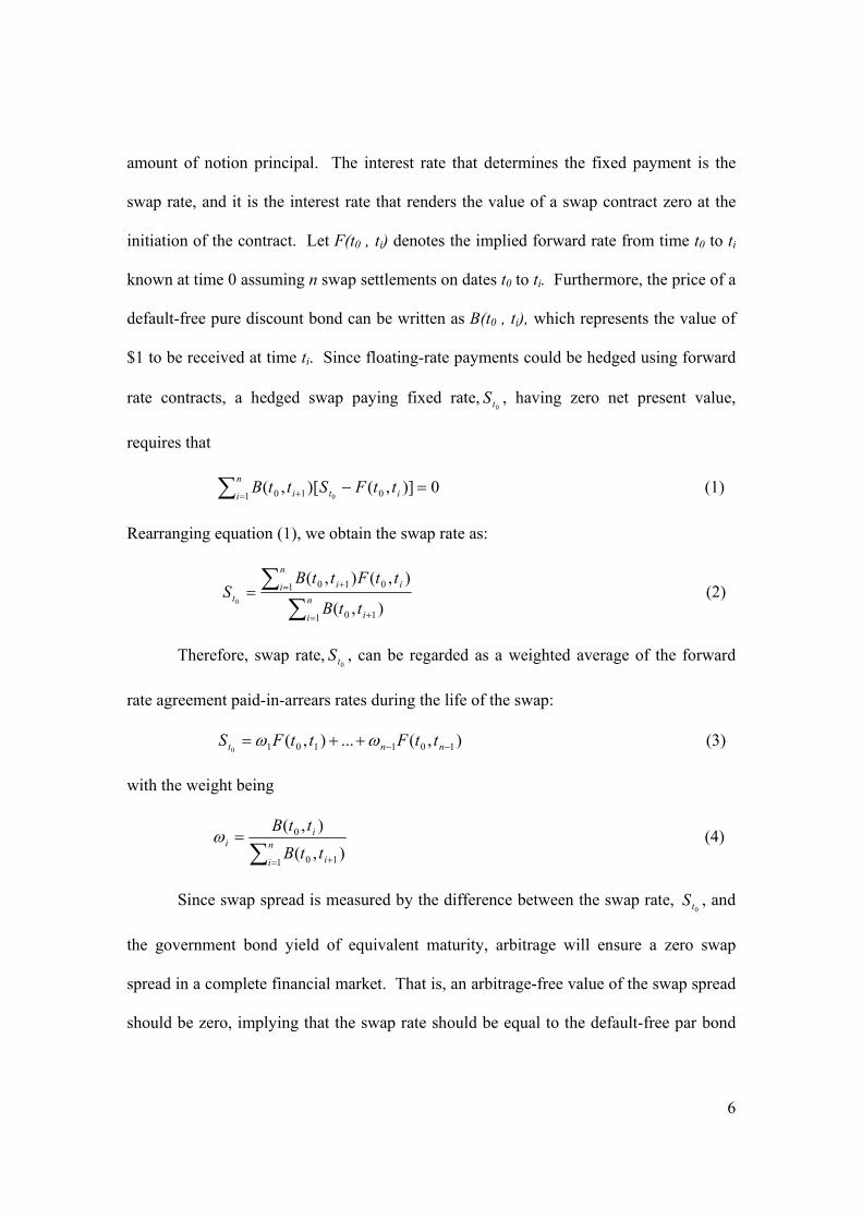
amount of notion principal. The interest rate that determines the fixed payment is the

swap rate, and it is the interest rate that renders the value of a swap contract zero at the

initiation of the contract. Let F(t0 , ti) denotes the implied forward rate from time t0 to ti

known at time 0 assuming n swap settlements on dates t0 to ti. Furthermore, the price of a

default-free pure discount bond can be written as B(t0 , ti), which represents the value of

$1 to be received at time ti. Since floating-rate payments could be hedged using forward

rate contracts, a hedged swap paying fixed rate,0t

S , having zero net present value,

requires that

0)],()[,(1 010 0

=−∑ = + in

i ti ttFSttB (1)

Rearranging equation (1), we obtain the swap rate as:

∑

∑= +

= += n

i i

n

i iit

ttB

ttFttBS

1 10

1 010

),(

),(),(0

(2)

Therefore, swap rate,0t

S , can be regarded as a weighted average of the forward

rate agreement paid-in-arrears rates during the life of the swap:

),(...),( 1011010 −−++= nnt ttFttFS ωω (3)

with the weight being

∑= +

= n

i i

ii

ttB

ttB

1 10

0

),(

),(ω (4)

Since swap spread is measured by the difference between the swap rate, 0t

S , and

the government bond yield of equivalent maturity, arbitrage will ensure a zero swap

spread in a complete financial market. That is, an arbitrage-free value of the swap spread

should be zero, implying that the swap rate should be equal to the default-free par bond

7

yield in the absence of market frictions. We will observe a non-zero swap spread,

however, when the financial markets are less than perfect, hence counterparty default risk

exists. Since the swap spread changes over time, it is important that we understand what

drives the dynamics of swap spread.

2.2 Literature review

Only in recent years researchers have begun to study the behavior of swap

spreads. Modeling interest rate swaps as a party who is short an option to receive (pay)

fixed and long an option to pay (receive) floating cash flows, with the counterparty

simultaneously owning the opposite pair of options, Sorensen and Bollier (1994) argue

that the value of a swap depends on the value of the option to default. The value of the

option to default, in turn, depends on a number of factors including the swap parties’

default probabilities, the shape of the yield curve, and interest rate volatility. Swap

spreads, therefore, are partially determined by the default risk which may be associated

with the interest rate volatility and the term structure of interest rate.

Grinblatt (2001), however, advances that generic swaps are default-free, and he

attributes the swap spread to the liquidity differences between government securities and

Eurodollar borrowings. Specifically, he contends that swap spreads contain a

convenience yield (liquidity premium) not available in the more liquid government

securities. Increases in liquidity premium, therefore, imply that the market requires a

higher premium to compensate for the reduced liquidity, which should result in a

corresponding increase in the swap spread. Collin-Dufresne and Solnik (2001), and He

(2002) echo the same argument because the net interest payment streams involved in the

swap are much smaller than in a bond.

8

Empirical evidence to date is far from conclusive. Minton (1997) finds that

bilateral counterparty default risk measured by corporate quality spread is not statistically

related to the swap rate. However, unilateral default risk measured by aggregate default

spread, exerts significant and positive impact on swap rate. Using VAR analyses, Huang

and Neftci (2006) find that liquidity risk, not default risk, is the primary driver of US

interest rate swap spreads. Liu, Longstaff, and Mandell (2006) report that the risk of

changes in the default probability is virtually not priced by the market. On the other hand,

employing impulse response function and variance decomposition method, Duffie and

Singleton (1997) conclude that both credit and liquidity risks have impact on the US

swap zero spread although the swap spread’s own innovation accounts for the majority of

the spread’s variations. Other studies examining the impact of liquidity and default risk

premiums on swap spreads include Brown et al. (1994), Lang et al. (1998), Sun et al.

(1993), and Fehle (2003). In addition to default and liquidity premiums, other economic

determinants of swap spreads by prior researches consist of interest rate volatility and

slope of the yield curve as they are alternative proxies of financial market risks (e.g., In et

al., 2003; Lekkos and Milas, 2001, 2004).

While most of the studies focus on the US swap rates and spreads, few examine

interest rate swaps of other currencies. Suhonen (1998) considers the determinants of

swap spreads in Finland and finds that spreads are positively related to the slope of the

yield curve and interest rate volatility. Lekkos and Milas (2001) study interest rate swaps

using both US and UK data. Lekkos and Milas (2004) model US and UK swap spreads

within an STVAR framework allowing for steep or flat yield curve slopes. Fang and

Muljono (2003) investigate Australian dollar interest rate swaps and conclude that the

9

spreads mostly represent a credit risk premium. In an unpublished working paper, Eom,

Subrahmanyam, and Uno (2000) study the credit risk and the Japanese yen interest rate

swap during the period of 1990-1996. They find that yen swap spreads behave very

differently from the credit spreads on Japanese corporate bonds, and overall the yen swap

market is sensitive to credit risk. Their study, however, only presents evidence on a time

period that is before the Japanese banking crisis and subsequent financial system reforms.

Most importantly, the majority of the swap rate studies rely upon OLS and linear VAR

analyses. Non-linear models in recent years have been proved to outperform the linear

ones, such as Lekkos and Milas (2004) and Lekkos et al. (2006), which find more flexible

interpretation of the results and provide better predictive power on swap spreads.

3. Data and Variables

Based upon the swap pricing model and the findings of extant literature, we

define and present relevant data in this section. Weekly data from August 8, 1997 to

April 15, 2005 are collected from Datastream and Bloomberg. Economic variables are

defined as follows:

SS2 ⎯ two-year maturity swap spreads; computed as the differential between the swap

rate and the Japan government bond (JGB) rate of two-year maturity.

SS5 ⎯ five-year maturity swap spreads; computed as the differential between the swap

rate and the Japan government bond rate of five-year maturity.

SS10 ⎯ ten-year maturity swap spread; computed as the differential between the swap

rate and the Japan government bond rate of ten-year maturity.

10

SLOPE ⎯ slope of the term structure; computed as the differential between the two-year

and the ten-year Japan government bond yields.

DEFAULT ⎯ default risk premium; computed as the differential between BBB rated 5-

year corporate bond yield and the Japan government bond yield of similar

maturity.

VOLATILITY ⎯ interest rate volatility fitted by a GARCH (1,1) model on 6-month

Japan government bond rates.4

LIQUIDITY ⎯ liquidity premium; computed by subtracting 6-month Japan government

bond rates from 6-month Japanese yen Tokyo Interbank Offered Rate (TIBOR).

JAPAN PREMIUM ⎯ the spread between TIBOR and LIBOR on Japanese yen.

Prior studies are followed in terms of measuring default risk. For example,

Minton (1997) uses corporate quality spread (BAA – AAA) and aggregate default spread

(BAA – T-Bond) to measure counterparty default risk. Duffie and Singleton (1997) use

the spread between BAA- and AAA-rated commercial paper rates, and Huang and Neftci

(2006) use the TED spread to measure credit risk. In a similar fashion, we collect yield

data on Japanese government bonds (JGB), AAA-rated, and BBB-rated corporate bonds.

However, since AAA-rated bonds have significant number of missing data, we employ

the spread between BBB-rated corporate bonds and JGB yields to proxy the default

premium.

We also include interest rate volatility generated by a GARCH model and the

slope of the term structure of interest rates in our empirical model because these two

variables determine the value of the option to default in the Sorensen and Bollier’s (1994)

4 An EGARCH model is discussed in In (2006).

11

model. Since increasing interest rate volatility is often associated with economic

uncertainty, as such, it is expected to positively influence swap spreads. Theoretically,

the impact of the slope of the term structure on swap spreads could be either positive or

negative. For instance, according to Sorensen and Bollier (1994), when the yield curve is

upward sloping, the fixed payer (floating receiver) is exposed to higher counterparty risk

due to higher default risk exposure associated with the higher future floating payments. A

lower fixed swap rate will compensate for this increased risk. Swap spreads are thus

expected to be negatively related to the slope of the term structure. On the other hand,

upward sloping yield curve normally coincides with strong economic growth, during

which bond credit premium tends to become larger (Alworth, 1993). In this case, swap

spreads are expected to be positively related to the slope of the term structure.

Following Grinblatt (2001) we measure liquidity premium by subtracting 6-month

JGB yield from similar maturity TIBOR rate. Since increasing convenience yield implies

that the market requires a higher premium to compensate for the decrease of liquidity in

TIBOR market, liquidity premium is also expected to be positively associated with swap

spreads. The variable JAPAN PREMIUM, computed as the spread between 6-month

TIBOR and LIBOR, is chosen to represent international financial markets’ assessment of

risks unique to Japan. During the period of Japanese banking crisis, Japanese banks

borrowing US dollars must pay a significant amount of premium.

Figure 1 provides plots of the above variables. Swap spreads are generally higher

and more volatile before 2001, and the term structure of swap spreads is upward sloping

with 10-year spreads the highest. There are also periods when 2-year spreads become

negative. After 2001, however, swap spreads are lower, less volatile, and the term

12

structure of swap spreads becomes inverted with 2-year and 5-year swap spreads higher

than the 10-year spreads. The periods of higher and more volatile swap spreads coincide

with the era that Japanese economy went through a recession and banking crisis. In late

1997, several reputable security firms including Sanyo Securities, Hokkaido Takushoku

Bank, Yamaichi Securities, and Tokuyo City Bank, announced the closure of their

business in a single month. Although the onset of the banking system trouble began in

1994 when credit cooperatives and housing finance companies (Jusen) encountered

serious financial problems, it is the unprecedented collapse of major banks that

propagated the rumors and shook the confidence of the entire Japanese financial system.

The credit ratings of banking firms rapidly degenerated during this period such that the

term Japan Premium, a premium on lending to Japanese institutions, appeared in the

international financial markets. In the JAPAN PREMIUM diagram, it is obvious that

larger premiums predominately appear in the periods of the late 1990s. By late 2000, the

new capital injection guided by the Financial Function Strengthening Law seemed to

have restored confidence in Japanese banks, hence the decline in premiums. The

magnitude of the premiums reduces to less than five basis points during the post banking

crisis period.5

Shown in the VOLATILITY diagram, volatilities are also much higher before

2001, but become minuscule after that. Interestingly, liquidity premiums also show

similar patterns. Before 2001, liquidity premiums are generally higher and more volatile,

but hovering around 10 basis points afterwards. Default premiums display those patterns

alike, although not as dramatic as the other economic determinants of swap spreads. The

5 For detailed discussions of the Japanese banking crisis, see Nakaso (2001), Miyajima and Yafeh (2003), and Krawczyk (2004).

13

only variable that does not exhibit a strong pattern is the slope of the JGB term structure.

Most of the time, the slope moves within a range between 100 and 160 basis points, with

two exceptions when it dips below 50 basis points.

Table 1 presents descriptive statistics of the economic variables employed in this

study. Panel A shows the statistics for the whole sample. It can be seen that the term

structure of swap spreads is upward sloping with SS10 the highest at 15.4 basis points,

SS5 at 11.7 basis points, and SS2 the lowest at 8 basis points. Considering the Japanese

economic conditions, the ex post patterns of swap spreads and their economic

determinants discussed above, we further partition the whole sample into two subperiods.

Panel B shows the statistics for the subperiod between August 1997 and December 2000,

while Panel C presents the same statistics for the second subperiod between January 2001

and April 2005.6 Consistent with Figure 1, default premium, Japan premium, liquidity

premium, and volatility are larger and more volatile (higher standard deviations) in the

first subperiod, reflecting the impact of the banking crisis. For swap spreads, both SS10

and SS5 are significantly higher in period 1. Average SS10 is 31 basis points in period 1,

but is less than 3 basis points in period 2 ― a tenfold difference. For the shorter-maturity

swap spread (SS2), the mean spreads are nearly identical in the two subperiods. These

preliminary statistics seem to suggest that longer-maturity swap spreads are more

sensitive to changing economic conditions.

4. Methodology

4.1. The baseline model

6 This preliminary sample partitioning for descriptive statistics in fact coincides with the test results of the regime shift reported in Section 5.

14

Since the sampling period used in this study encompasses different economic

regimes, a linear VAR may not be the appropriate model to use. In this section, we

consider the VAR extension of the smooth transition autoregressive (STVAR) model in

Camacho (2004), which is also employed in Lekkos and Milas (2004), and Lekkos et al.

(2006). The model permits a smooth transition of regimes based upon an empirically

chosen economic factor. Let

( ) ( )1 1 ,( ) ( )t t t i t d tY A B L Y C D L Y F Y u− − −= + + + + , (5)

where Yt represents a time-series vector including swap spreads (SS2, SS5, or SS10),

slope of the term structure (SLOPE), default premiums (DEFAULT), liquidity premiums

(LIQUIDITY), Japan premiums (JAPAN PREMIUM), and interest rate volatilities

(VOLATILITY). A and C are vectors of intercepts, B(L) and D(L) are polynomial

matrices of p-th order lag, d is the delay parameter, and ut follows an independent and

identically distributed Gaussian process with zero mean and variance Ω.

The key component of this STVAR system is the transition function F(• ), which

controls the regime switching and is bounded between zero and one. When F(• ) is zero,

equation (5) becomes a linear VAR (VAR-a) with parameters A and B(L). On the

contrary, when F(• ) is one, the model becomes a different linear VAR (VAR-b) with

parameters A+C and B(L)+D(L). Hence, F(• ) may be interpreted as a filtering rule that

locates the model between these two extreme regimes. Until these regimes can be

interpreted economically, we will refer to them as “first regime” and “second regime”,

respectively.

15

In order to consider different forms of transition across these regimes, two

transition functions have been developed in the literature. The first one is the logistic

function, stated as:

( ) ( ) ,/]exp[1 1

,,−

−− −−+= σγ cYYF dtidti (6) where c is the threshold between two regimes, and σ is the standard deviation of Yi,t-d.

The second one is the exponential transition function, which can be written as:

( ) ( )2 2

, ,1 exp[ / ]i t d i t dF Y Y cγ σ− −= − − − . (7)

When the transition function ,( )i t dF Y − is set to be logistic, it changes

monotonically from the first regime to the second regime with transition value Yi,t-d. The

transition function becomes a constant when g → 0, and the transition from 0 to 1 is

instantaneous at Yi,t-d = c when g → +∞. On the other hand, under the exponential

function, the system changes symmetrically relative to the threshold c with Yi,t-d, but the

model turns linear if either g → 0 or g → +∞. In both models, the smoothness parameter

γ, which is restricted to be positive between zero and one, controls the speed of

adjustment across regimes.

4.2. Linearity tests and the transition function

We follow the specification suggested in Camacho (2004), which adapts the

univariate proposal of Granger and Terasvirta (1993) to a multi-equation context, for the

empirical examination of the behavior of Japanese Yen swap spreads.

The first step of the estimation is to specify a linear VAR model as the basis to

obtain the nonlinear results. This is because even if the true model is nonlinear, the linear

16

specification is a simpler framework to obtain preliminary results that may assist in

obtaining the set of variables to include in the nonlinear specification. In a small-scale

system, linear specification may also help us to decide the maximum lag length p. In a

large-scale system, however, the selection of p may be constrained to consider a tractable

number of parameters to be estimated. Since our system contains six variables, we restrict

our analysis to VAR models of order one. Estimations based upon higher order VARs

have also been tried but they fail to converge in the non-linear models.

Next, some linearity and model selection tests are conducted. Maximum

likelihood method is employed for the estimation, in which (2 × the log likelihood under

the alternative − the log likelihood under the null) will follow asymptotically a χ2

distribution with degrees of freedom equal to the number of restrictions imposed under

the null.7

Assuming that d is known, testing linearity is still nonstandard due to the presence

of nuisance parameters. Following the suggestions of Luukkonen, Saikkonen and

Teräsvirta (1988), the problem may be overcome by suitable Taylor approximations of

the transition function around γ = 0. Assuming p = 1, the problem of testing linearity is

reduced to estimating the following auxiliary regression:

2 30 1 1 1 , 2 1 , 3 1 ,t t t i t d t i t d t i t d tY g G Y G Y Y G Y Y G Y Y ε− − − − − − −= + + + + + (8)

for each transition variable candidate i = 1,2,…,6, and to test

0: 3210 === GGGH .

In empirical applications, d is usually restricted to be less than or equal to p,

therefore, we consider just one lag for each candidate of the transition variable. Linearity

7 See Camacho (2004) for technical details about maximum likelihood estimation.

17

tests are applied for each of these lagged variables. In case of multiple rejections of the

null, we follow Terasvirta (1994) such that the lagged variable with the highest rejection

of linearity (i.e. the largest statistic or the lowest p-value) is chosen as the most suitable

transition variable.

Our results of linearity tests appear in Table 2. The null of linearity is essentially

rejected in all variables with the exception of lagged swap spreads in the SS5 model.

Hence it confirms that a non-linear model better fits our Japanese swap data. The

following step is to choose the transition variable. In order to select just one transition

variable that is responsible for the regime shift in the nonlinear model, we also show the

ratio of the linearity test statistic for each candidate over the statistic that corresponds to

VOLATILITY, which has the largest statistic across all spread maturities. Accordingly,

lagged volatility is adopted as the transition variable in the transition function.

After determining the delay parameter d and the transition variable that governs

the transition across regimes, the third step is to choose between a logistic and an

exponential form of the transition function. The tests that are sequentially applied to the

auxiliary regression (i.e. 01H , 02H , and 03H , respectively) and subsequent decisions are

illustrated in Table 3. Using lagged volatility as the transition variable, the p-values of

Test 1, Test 2 and Test 3 are all about 0.000. Therefore, we conclude that the appropriate

transition function is logistic.

5. Empirical Results 5.1. Regime identification

18

The logistic transition function model is now estimated using the maximum

likelihood method.8 For the ease of presentation and to shed some lights on the

nonlinearities obtained in the model, Figure 2 plots the transition function against lagged

volatility for all swap maturities. The estimates of the speed of transition (γ) between

regimes and the threshold parameter (c) are also reported in the notes under each panel.

The transition function suggests that the “first regime” (F close to one) is associated with

periods of high volatility whereas the “second regime” (F close to zero) is classified as

the low volatility regime. The estimated threshold levels (c) are about 0.08, 0.10, and

0.12, which mark the halfway point between regimes, for SS2, SS5, and SS10

respectively. The estimated smoothness parameters (γ ), which determine the velocity of

transition between these two states, are close to 4 for all swap maturities with minor

variations.

Figure 3 plots the values of the transition function (solid line, left-hand axis) and

VOLATILITY (line with blocks, right-hand axis) for all swap maturities. It is clearly

shown that high values of the transition function F are associated with occurrence of high

volatility from 1997 to 2000. From 2001 to 2005, however, the transition function falls

dramatically to almost zero which corresponds to a long period of low volatility. It should

be noted that the break point between regimes occurs near the end of the Japanese

banking crisis.

5.2. Generalized impulse response analysis

In this subsection, we explain the estimation procedure of the generalized impulse

response function (GIRF), and report associated empirical results for our STVAR

8 Parameter estimates are not reported to save space. They are available from the authors upon request.

19

models. Since impulse responses identify the consequences of an increase in the jth

variable innovation at date t for the value of the ith variable at time t+h, the GIRF of the

STVAR model traces the time path where the swap spread returns to equilibrium after an

economic shock is injected into the system. The visual aids provided by the impulse

response functions are particularly useful when the full impact of economic shocks on

swap spreads takes long lags to materialize.

In the nonlinear context, however, these effects not only depend on the shocks

that occur between t and t+h, but also on the past shock history, wt-1. Following Weise

(1999), we define the generalized impulse response function of variable i for an arbitrary

shock to variable j denoted by εjt = δj and history wt-1 as:

( ) ( ) ( )1,1,1 /,/,, −+−+− −== thtitjjthtitj wYEwYEwhGIRF δεδ . (9)

In the empirical application, δj is set to one standard deviation of variable j. In

other words, the shock to each equation is equal to one standard deviation of the equation

residual. Note that, in linear contexts, shocks between t and t+h are usually set to zero for

convenience. As documented by Koop, Pesaran and Potter (1996), this approach is not

appropriate in the context of nonlinear models.9 In order to deal with the problem of

shocks in intermediate time periods, we follow the bootstrap procedure suggested by

Weise (1999). We first obtain 5000 draws with replacements from the residuals of the

nonlinear model, compute the GIRF for each of them and then average the responses. In

9 In linear models, impulse responses of variable i to shocks in variable j can be defined as the difference between realizations of Yi,,t+h and a baseline “no shock” scenario:

( ) ( ) ( )1,0,...,0/,1,0,...,01,/,1,, −=+=+−−=+=+=+=− twhjtjthtiYEtwhjtjtjjthtiYEtwjhIRF εεεεδεδ

where δ is set to one standard deviation of variable j. Note that all shocks in intermediate periods between t and t+h are set equal to zero. This is because the expectation of the path of Y following a shock, conditional on the future shocks, is equal to the path of the variable when future shocks are set to their expected values. Therefore, future shocks can be set equal to zero for convenience.

20

addition, GIRFs are history dependent. To account for this dependency, we compute the

GIRFs conditional on two particular histories of wt-1, namely, the periods that correspond

to Ft = 0.85, a high volatility regime; and Ft = 0.15, a low volatility regime.10 As such, this

allows us to compare the responses of shocks that hit the economy in two distinct

regimes. Indeed, this is the advantage of nonlinear VAR models that incorporate the

asymmetric effects of economic shocks on swap spreads across different regimes.

To contrast the difference between regimes, the impulse responses of SS2 to

shocks imposed on various economic variables are presented in Figures 4 and 5

respectively for the high and low volatility regimes. Several dissimilarities between

regimes stand out. First, swap spreads are generally more responsive to economic shocks

in the high volatility regime. For example, in the first regime a shock on default premium

generates a positive impact on SS2, which peaks at approximately one basis point in

week seven, and the impact gradually dies out in about 40 weeks. A similar shock in the

second regime only provokes a response less than 0.4 bps from SS2. Although differing

in magnitude, the positive impact of default shock on swap spreads is consistent with a

priori expectations.

Similar observations can be found in swap spreads from a shock emanating from

volatility. SS2 reacts stronger to a volatility shock in the first regime than in the second.

The positive response of SS2 peaks out at 0.4 bps in about five weeks, leveling off in

about 35 weeks in the high volatility regime. By contrast, in the low volatility regime,

the response is merely less than half of the response in the first regime and rapidly

disappears in about five weeks. The impulse response of SS2 to the term structure shock

10 Imposing starting points of F exactly equal to either 1 or 0 is not empirically plausible since we need enough observations in the right and left hand sides of the distribution.

21

also displays an asymmetric pattern. A positive, though small response is observed in the

first regime, which is in agreement with the findings reported in Alworth (1993) for the

US dollar swap spreads, and Suhonen (1998) for Finland data. The swap spread’s

response to the term structure shock, however, is virtually nil in the second regime. The

responses of SS2 to liquidity premium and Japan premium also exhibit regime-

dependent, asymmetric patterns, although not as dramatic as those invoked by shocks

from default premium and volatility. The effects of swap spreads from the shock in Japan

premium are by far the smallest among all.

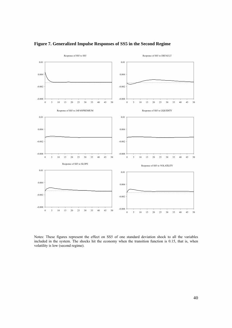
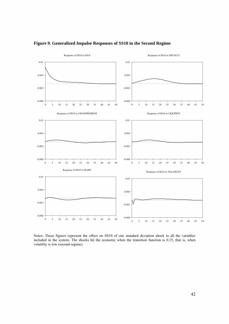
In a similar fashion, the impulse responses of SS5 and SS10 to the economic

shocks in different regimes are presented in Figures 6, 7, 8, and 9 respectively. Again,

swap spreads appear to be more responsive to economic shocks when the high volatility

regime dominates, and no significant responses are uncovered in the low volatility

regime.

Our model also successfully captures differential responses in swap spreads

across different maturities. We use the impulse response results for SS5 in the high

volatility regime to illustrate these differences. First of all, the response of swap spreads

to the default shock is more pronounced for the shorter-term swap (i.e., SS2). The peak

response of SS2 to default shock is one bp, while it is approximately half of this

magnitude for SS5. Similar effects are also revealed in the results for the volatility

shock, where SS2 is more responsive to the volatility shock than SS5. Conversely, the

response of SS5 to the term structure shock, the opposite is true. That is, the magnitude

of the response of SS5 to the default shock is twice that of SS2. This is similar to the

findings in other studies (e.g., Lekkos and Milas, 2004). This result stems from the fact

22

that the exposure to the possibility of default (from the floating-rate payer in the swap

deal) for the fixed rate payer is higher during the later stage of the contract, hence higher

embedded risks for the longer-term contracts.

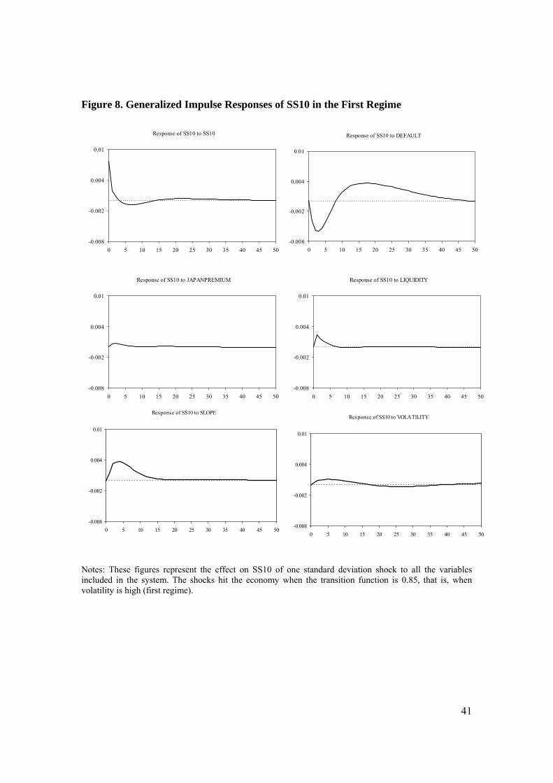
In terms of 10-year swap spreads, the difference in responses due to maturities is

particularly manifest in shocks from default, liquidity and term structure slope risks.

Other than default shocks, responses of SS10 to shocks emanating from other variables

more resemble those of SS5 than SS2. Distinct from shorter-maturity swap spreads, in

the high volatility regime SS10 initially declines following a default shock, but the

response reverts to be positive seven weeks thereafter. This result seems to be somehow

related to Eom et al’s (2000) finding of a negative covariance between the default-free

rate and the swap spread in Japan during this period. Our result may be consistent with

their finding if the correlation between BBB-bond yields and JGB yields is positive.11

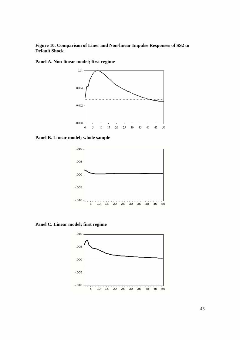
5.3. Comparison of non-linear and liner impulse response functions

In this subsection, we show that results can differ substantially between linear and

nonlinear models. To save space, Figures 10 and 11 only exhibit the impulse responses

of swap spreads to default shocks and spreads’ own shocks. In Panel A of Figure 10, the

response of SS2 to default shock in the high volatility regime from the non-linear model

is presented for contrasting purpose. Panel B plots the response of SS2 to default shock

in a linear model for the entire sample from 1997 to 2005 without considering the shift in

regimes. The two panels reveal drastic differences in impulse responses. The significant

impact of default shock on SS2 in the non-linear model is completely absent in the linear

11 We also run an OLS regression with all economic determinants and lagged SS10 (one lag) as the exogenous variables to ensure that our finding is not methodology-driven. The OLS results show a negative relation between default premium and swap spreads during this sample period.

23

model. Panel C indicates that the linear model also fails to capture the acute response of

SS2 to default shock during the first regime.

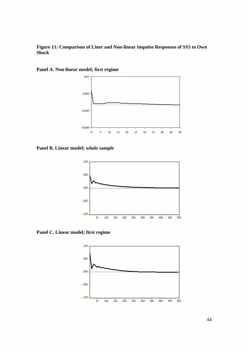
In Figure 11, we present the responses of SS5 to its own shock based upon non-

linear and linear models. In Panel A, the high volatility regime witnesses a rather short-

lived, diminutive reaction of SS5 to its own shock in the non-linear model. However, the

linear model depicted in Panel B demonstrates that for the whole sample the long-lasting

impact does not die out until 30 weeks later. Evident in Panel C, the linear impulse

response of SS5 to its own shock under the first regime suggests that the effect persists

over a long horizon. The STVAR results thus help us avoid any fallacious conclusions

due to a linear model specification.

6. Conclusions

In this paper we model the nonlinear relationship of Japanese yen interest rate

swap spreads and a number of risk factors within a smooth transition VAR framework.

Weekly data for the 2-year, 5-year and 10-year swap spreads and corresponding

economic determinants of swap spreads, namely default premium, liquidity premium, the

term structure slope, Japan premium, and interest rate volatility, are obtained from 1997

to 2005 for this purpose. Our nonlinear model enables us to capture a time-varying

component of swap spreads across different maturities. The non-linear dynamics are

corroborated by the fact that swap spreads of all maturities are very volatile and large in

magnitude during the period of Japanese banking crisis, but become much smaller and

more stable during the post banking crisis period. Most of the swap spread determinants

exhibit signs of a regime shift as well.

24

Linearity tests reject the linear model in favor of a non-linear VAR, and the model

selection tests conclude that a logistic transition function better fits the data. Interest rate

volatility is identified as the transition variable responsible for the shift of regimes. The

estimated transition function suggests that the “first regime” is associated with periods of

high volatility whereas the “second regime” corresponds to periods of low volatility.

Incidentally, this break point occurs near the end of the Japanese banking crisis.

Generalized impulse response functions help analyze the time paths of the impact

of economic shocks on swap spreads of various maturities across regimes. Three major

conclusions are in order. First, a regime effect is present during the period we study.

Swap spreads of all maturities are more responsive to economic shocks in the high

volatility regime when Japan was going through a banking crisis. It is found that the

magnitude of the peak response of SS2 to default and volatility shocks in the high

volatility regime is more than twice of that in the low volatility regime. The

corresponding response of SS2 to a term structure shock can be hardly detected in the

second regime. Second, a maturity effect is implied in the variability of swap spreads

across regimes. Dissimilarities in responses are observed between the short-end of the

swap maturity (SS2) and the longer-end (SS5 and SS10). It is evident from our estimation

that SS2 is more responsive to the volatility shock than SS5 or SS10. Impulse responses

of swap spreads to the term structure shock exhibit an opposite pattern, with longer

maturity swaps more sensitive. This finding is consistent with the notion that the

exposure to default risks for the fixed rate payer increases during the later stage of the

contract, hence higher embedded risks. Last, and most importantly, fallacious conclusions

of a liner VAR are avoided under the STVAR framework.

25

References

Alworth, J.S., 1993. The valuation of US dollar interest rate swaps, BIS Economic Papers, 35, January. Brown, K.C., W.V. Harlow, and D.J. Smith, 1994. An empirical analysis of interest rate swap spreads. Journal of Fixed Income 3, 61-78. Camacho, M., 2004. Vector smooth transition regression models for US GDP and the composite index of leading indicators. Journal of Forecasting 23, 173-196. Collin-Dufresne, P. and B. Solnik, 2001. On the term structure of default premia in the swap and LIBOR markets. Journal of Finance 56, 1095-1115. Duffie, D., and K.J. Singleton, 1997. An econometric model of the term structure of interest rate swap yields. Journal of Finance 52, 1287-1321. Eom, Y.H., M.G. Subrahmanyam, and J. Uno, 2000. Credit risk and the yen interest rate swap market. Working paper, Stern School of Business, New York University. Fang, V., and R. Muljono, 2003. An empirical analysis of the Australian dollar swap spreads. Pacific-Basin Finance Journal 11, 153-173. Fehle, F., 2003. The components of interest rate swap spreads: theory and international evidence. Journal of Futures Markets 23, 347-387. Granger C, and T. Teräsvirta, 1993. Modeling nonlinear economic relationships. Oxford University Press: New York. Grinblatt, M., 2001. An analytical solution for interest rate swap spreads. International Review of Finance 2 (3), 113-149. He, H., 2000. Modeling term structures of swap spreads. Working paper, Yale School of Management. Huang, Y., and S. Neftci, 2006. Modeling swap spreads: the roles of credit, liquidity and market volatility. Review of Futures Market 14, 431-450. In, F., R. Brown, and V. Fang, 2003. Modeling volatility and changes in the swap spread. International Review of Financial Analysis 12, 545-561. In, F., 2006. Volatility spillovers across international swap markets: the US, Japan, and the UK. Journal of International Money and Finance (forthcoming). Koop, G., M. Pesaran, and S. Potter, 1996. Impulse response analysis in nonlinear multivariate models. Journal of Econometrics 74, 119-147.

26

Krawczyk, M.K., 2004. Change and crisis in the Japanese banking industry. HWWA discussion paper 277, Hamburg Institute of International Economics. Lang, L.H.P., R.H. Litzenberger, and A.L. Liu, 1998. Determinants of interest rate swap spreads. Journal of Banking and Finance 22, 1507-1532. Lekkos, I., and C. Milas, 2001. Identifying the factors that affect interest-rate swap spreads: some evidence from the United States and the United Kingdom. Journal of Futures Markets 21, 737-768. _____________________, 2004. Common risk factors in the US and UK interest rate swap markets: evidence from a non-linear vector autoregression approach. Journal of Futures Markets 24, 221-250. Lekkos, I., C. Milas, and T. Panagiotidis, 2006. Forecasting interest rate swap spreads using domestic and international risk factors: evidence from linear and non-linear models. Journal of Forecasting, forthcoming. Liu, J., F.A. Longstaff, and R.E. Mandell, 2006. The market price of risk in interest rate swaps: the roles of default and liquidity risks. Journal of Business 79 (5), 2337-2360. Luukkonen R., P. Saikkonen, and T.Teräsvirta, 1988. Testing linearity against smooth transition autoregressive models. Biometrika 75, 491-499. Minton, B., 1997. An empirical examination of basic valuation models for plain vanilla US interest rate swaps. Journal of Financial Economics 44, 251-277. Miyajima, H., and Y. Yafeh, 2003. Japan’s banking crisis: who has the most to lose? CEI Working Paper Series 15, Hitotsubashi University. Nakaso, H., 2001. The financial crisis in Japan during the 1990s: how the Bank of Japan responded and the lessons learnt. BIS Papers, No. 6. Pesaran, H., and Y. Shin, 1998. Impulse response analysis in linear multivariate models. Economics Letters 58, 165-193. Sorensen, E.H., and T.F. Bollier, 1994. Pricing swap default risk. Financial Analysts Journal 50, 23-33. Suhonen, A., 1998. Determinants of swap spreads in a developing financial markets: evidence from Finland. European Financial Management 4, 379-399. Sun, T.S., S. Sundaresan, and C. Wang, 1993. Interest rate swaps – an empirical investigation. Journal of Financial Economics 34, 77-99.

27

Teräsvirta T., 1994. Specification, estimation and evaluation of smooth transition autoregressive models. Journal of the American Statistical Association 89, 208-18. Weise C., 1999. The asymmetric effects of monetary policy: a nonlinear vector autoregression approach. Journal of Money, Credit and Banking 31, 85-108.

28

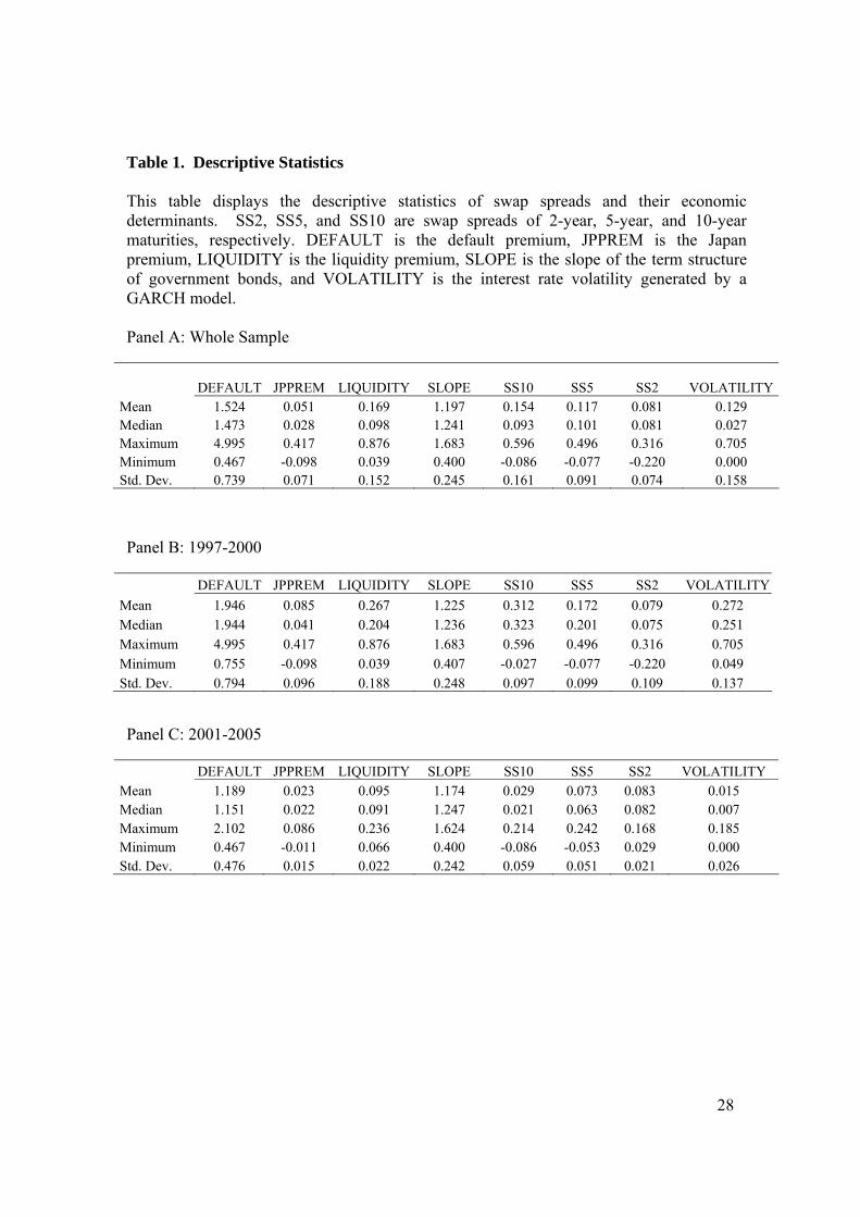
Table 1. Descriptive Statistics This table displays the descriptive statistics of swap spreads and their economic determinants. SS2, SS5, and SS10 are swap spreads of 2-year, 5-year, and 10-year maturities, respectively. DEFAULT is the default premium, JPPREM is the Japan premium, LIQUIDITY is the liquidity premium, SLOPE is the slope of the term structure of government bonds, and VOLATILITY is the interest rate volatility generated by a GARCH model. Panel A: Whole Sample

DEFAULT JPPREM LIQUIDITY SLOPE SS10 SS5 SS2

VOLATILITY Mean 1.524 0.051 0.169 1.197 0.154 0.117 0.081 0.129 Median 1.473 0.028 0.098 1.241 0.093 0.101 0.081 0.027 Maximum 4.995 0.417 0.876 1.683 0.596 0.496 0.316 0.705 Minimum 0.467 -0.098 0.039 0.400 -0.086 -0.077 -0.220 0.000 Std. Dev. 0.739 0.071 0.152 0.245 0.161 0.091 0.074 0.158

Panel B: 1997-2000

DEFAULT JPPREM LIQUIDITY SLOPE SS10 SS5 SS2 VOLATILITY Mean 1.946 0.085 0.267 1.225 0.312 0.172 0.079 0.272 Median 1.944 0.041 0.204 1.236 0.323 0.201 0.075 0.251 Maximum 4.995 0.417 0.876 1.683 0.596 0.496 0.316 0.705 Minimum 0.755 -0.098 0.039 0.407 -0.027 -0.077 -0.220 0.049 Std. Dev. 0.794 0.096 0.188 0.248 0.097 0.099 0.109 0.137

Panel C: 2001-2005

DEFAULT JPPREM LIQUIDITY SLOPE SS10 SS5 SS2 VOLATILITY Mean 1.189 0.023 0.095 1.174 0.029 0.073 0.083 0.015 Median 1.151 0.022 0.091 1.247 0.021 0.063 0.082 0.007 Maximum 2.102 0.086 0.236 1.624 0.214 0.242 0.168 0.185 Minimum 0.467 -0.011 0.066 0.400 -0.086 -0.053 0.029 0.000 Std. Dev. 0.476 0.015 0.022 0.242 0.059 0.051 0.021 0.026

29

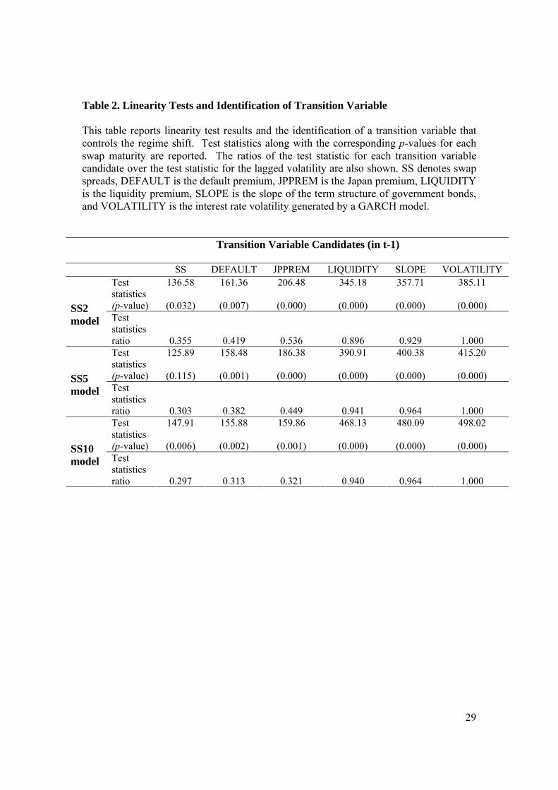
Table 2. Linearity Tests and Identification of Transition Variable This table reports linearity test results and the identification of a transition variable that controls the regime shift. Test statistics along with the corresponding p-values for each swap maturity are reported. The ratios of the test statistic for each transition variable candidate over the test statistic for the lagged volatility are also shown. SS denotes swap spreads, DEFAULT is the default premium, JPPREM is the Japan premium, LIQUIDITY is the liquidity premium, SLOPE is the slope of the term structure of government bonds, and VOLATILITY is the interest rate volatility generated by a GARCH model.

Transition Variable Candidates (in t-1)

SS DEFAULT JPPREM LIQUIDITY SLOPE VOLATILITY Test statistics (p-value)

136.58

(0.032)

161.36

(0.007)

206.48

(0.000)

345.18

(0.000)

357.71

(0.000)

385.11

(0.000)

SS2 model Test

statistics ratio

0.355

0.419

0.536

0.896

0.929

1.000 Test statistics (p-value)

125.89

(0.115)

158.48

(0.001)

186.38

(0.000)

390.91

(0.000)

400.38

(0.000)

415.20

(0.000)

SS5 model Test

statistics ratio

0.303

0.382

0.449

0.941

0.964

1.000 Test statistics (p-value)

147.91

(0.006)

155.88

(0.002)

159.86

(0.001)

468.13

(0.000)

480.09

(0.000)

498.02

(0.000)

SS10 model

Test statistics ratio

0.297

0.313

0.321

0.940

0.964

1.000

30

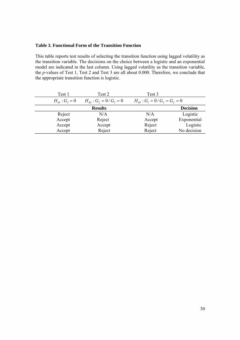
Table 3. Functional Form of the Transition Function This table reports test results of selecting the transition function using lagged volatility as the transition variable. The decisions on the choice between a logistic and an exponential model are indicated in the last column. Using lagged volatility as the transition variable, the p-values of Test 1, Test 2 and Test 3 are all about 0.000. Therefore, we conclude that the appropriate transition function is logistic. Test 1 Test 2 Test 3 0: 301 =GH 0/0: 3202 == GGH 0/0: 23103 === GGGH Results Decision Reject N/A N/A Logistic Accept Reject Accept Exponential Accept Accept Reject Logistic Accept Reject Reject No decision

31

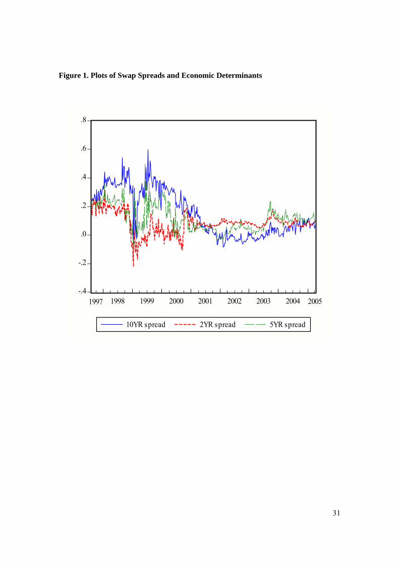
Figure 1. Plots of Swap Spreads and Economic Determinants

-.4

-.2

.0

.2

.4

.6

.8

1998 1999 2000 2001 2002 2003 2004

10YR spread 2YR spread 5YR spread

1997 2005

32

Figure 1. (Continued)

DEFAULT

0

1

2

3

4

5

6

1997 1998 1999 2000 2001 2002 2003 2004 2005

JAPAN PREMIUM

-0.2

-0.1

0

0.1

0.2

0.3

0.4

0.5

1997 1998 1999 2000 2001 2002 2003 2004 2005

LIQUIDITY

0

0.1

0.2

0.3

0.4

0.5

0.6

0.7

0.8

0.9

1997 1998 1999 2000 2001 2002 2003 2004 2005

SLOPE

0.2

0.4

0.6

0.8

1

1.2

1.4

1.6

1.8

1997 1998 1999 2000 2001 2002 2003 2004 2005

VOLATILITY

0

0.2

0.4

0.6

0.8

1

1997 1998 1999 2000 2001 2002 2003 2004 2005

Figure 2. Estimated Transition Function (Vertical Axis) against VOLATILITY (Horizontal Axis) at t-1 Panel A: SS2

Notes: The first regime (F close to one) is interpreted as periods where volatility is high whereas the second regime (F close to zero) can be seen as periods associated with relatively low volatility. The estimated transition function is F(Vt-1)=1+ exp[-3.92(Vt-1-0.08)/σ]-1, where V refers to volatility and σ is its standard deviation. Panel B: SS5

Notes: The first regime (F close to one) is interpreted as periods where volatility is high whereas the second regime (F close to zero) can be seen as periods associated with relatively low volatility. The estimated transition function is F(Vt-1)= 1+ exp[-3.80(Vt-1-0.10)/σ]-1, where V refers to volatility and σ is its standard deviation.

0

0.2

0.4

0.6

0.8

1

0 0.1 0.2 0.3 0.4 0.5 0.6 0.7 0.8

0

0.2

0.4

0.6

0.8

1

0 0.1 0.2 0.3 0.4 0.5 0.6 0.7 0.8

34

Panel C: SS10

Notes: The first regime (F close to one) is interpreted as periods where volatility is high whereas the second regime (F close to zero) can be seen as periods associated with relatively low volatility. The estimated transition function is F(Vt-1)= 1+ exp[-4.01(Vt-1-0.12)/σ]-1, where V refers to volatility and σ is its standard deviation.

0

0.2

0.4

0.6

0.8

1

0 0.1 0.2 0.3 0.4 0.5 0.6 0.7 0.8

35

Figure 3. Transition Function and VOLATILITY

Panel A: SS2

Panel B: SS5

0

0.2

0.4

0.6

0.8

1

1997 1998 1999 2000 2001 2002 2003 2004 20050

0.2

0.4

0.6

0.8

1

0

0.2

0.4

0.6

0.8

1

1997 1998 1999 2000 2001 2002 2003 2004 20050

0.2

0.4

0.6

0.8

1

36

Panel C: SS10

Notes: The transition function is the solid line (left-hand axis) and volatility is the line with blocks (right-hand axis). Values of the transition function close to one refer to the first regime and correspond to periods of high volatility. Note that the break point is at about the end of the banking crisis, a time period characterized with rapid reduction in volatility.

0

0.2

0.4

0.6

0.8

1

1997 1998 1999 2000 2001 2002 2003 2004 20050

0.2

0.4

0.6

0.8

1

37

Figure 4. Generalized Impulse Responses of SS2 in the First Regime

Notes: These figures represent the effect on SS2 of one standard deviation shock to all the variables included in the system. The shocks hit the economy when the transition function is 0.85, that is, when volatility is high (first regime).

Response of SS2 to SS2

-0.008

-0.002

0.004

0.01

0 5 10 15 20 25 30 35 40 45 50

Response of SS2 to DEFAULT

-0.008

-0.002

0.004

0.01

0 5 10 15 20 25 30 35 40 45 50

Response of SS2 to JAPANPREMIUM

-0.008

-0.002

0.004

0.01

0 5 10 15 20 25 30 35 40 45 50

Response of SS2 to LIQUIDITY

-0.008

-0.002

0.004

0.01

0 5 10 15 20 25 30 35 40 45 50

Response of SS2 to SLOPE

-0.008

-0.002

0.004

0.01

0 5 10 15 20 25 30 35 40 45 50

Response of SS2 to VOLATILITY

-0.008

-0.002

0.004

0.01

0 5 10 15 20 25 30 35 40 45 50

38

Figure 5. Generalized Impulse Responses of SS2 in the Second Regime

Notes: These figures represent the effect on SS2 of one standard deviation shock to all the variables included in the system. The shocks hit the economy when the transition function is 0.15, that is, when volatility is low (second regime).

Response of SS2 to SS2

-0.008

-0.002

0.004

0.01

0 5 10 15 20 25 30 35 40 45 50

Response of SS2 to DEFAULT

-0.008

-0.002

0.004

0.01

0 5 10 15 20 25 30 35 40 45 50

Response of SS2 to JAPANPREMIUM

-0.008

-0.002

0.004

0.01

0 5 10 15 20 25 30 35 40 45 50

Response of SS2 to LIQUIDITY

-0.008

-0.002

0.004

0.01

0 5 10 15 20 25 30 35 40 45 50

Response of SS2 to SLOPE

-0.008

-0.002

0.004

0.01

0 5 10 15 20 25 30 35 40 45 50

Response of SS2 to VOLATILITY

-0.008

-0.002

0.004

0.01

0 5 10 15 20 25 30 35 40 45 50

39

Figure 6. Generalized Impulse Responses of SS5 in the First Regime

Notes: These figures represent the effect on SS5 of one standard deviation shock to all the variables included in the system. The shocks hit the economy when the transition function is 0.85, that is, when volatility is high (first regime).

Response of SS5 to SS5

-0.008

-0.002

0.004

0.01

0 5 10 15 20 25 30 35 40 45 50

Response of SS5 to DEFAULT

-0.008

-0.002

0.004

0.01

0 5 10 15 20 25 30 35 40 45 50

Response of SS5 to JAPANPREMIUM

-0.008

-0.002

0.004

0.01

0 5 10 15 20 25 30 35 40 45 50

Response of SS5 to LIQUIDITY

-0.008

-0.002

0.004

0.01

0 5 10 15 20 25 30 35 40 45 50

Response of SS5 to SLOPE

-0.008

-0.002

0.004

0.01

0 5 10 15 20 25 30 35 40 45 50

Response of SS5 to VOLATILITY

-0.008

-0.002

0.004

0.01

0 5 10 15 20 25 30 35 40 45 50

40

Figure 7. Generalized Impulse Responses of SS5 in the Second Regime

Notes: These figures represent the effect on SS5 of one standard deviation shock to all the variables included in the system. The shocks hit the economy when the transition function is 0.15, that is, when volatility is low (second regime).

Response of SS5 to SS5

-0.008

-0.002

0.004

0.01

0 5 10 15 20 25 30 35 40 45 50

Response of SS5 to DEFAULT

-0.008

-0.002

0.004

0.01

0 5 10 15 20 25 30 35 40 45 50

Response of SS5 to JAPANPREMIUM

-0.008

-0.002

0.004

0.01

0 5 10 15 20 25 30 35 40 45 50

Response of SS5 to LIQUIDITY

-0.008

-0.002

0.004

0.01

0 5 10 15 20 25 30 35 40 45 50

Response of SS5 to SLOPE

-0.008

-0.002

0.004

0.01

0 5 10 15 20 25 30 35 40 45 50

Response of SS5 to VOLATILITY

-0.008

-0.002

0.004

0.01

0 5 10 15 20 25 30 35 40 45 50

41

Figure 8. Generalized Impulse Responses of SS10 in the First Regime

Notes: These figures represent the effect on SS10 of one standard deviation shock to all the variables included in the system. The shocks hit the economy when the transition function is 0.85, that is, when volatility is high (first regime).

Response of SS10 to SS10

-0.008

-0.002

0.004

0.01

0 5 10 15 20 25 30 35 40 45 50

Response of SS10 to DEFAULT

-0.008

-0.002

0.004

0.01

0 5 10 15 20 25 30 35 40 45 50

Response of SS10 to JAPANPREMIUM

-0.008

-0.002

0.004

0.01

0 5 10 15 20 25 30 35 40 45 50

Response of SS10 to LIQUIDITY

-0.008

-0.002

0.004

0.01

0 5 10 15 20 25 30 35 40 45 50

Response of SS10 to SLOPE

-0.008

-0.002

0.004

0.01

0 5 10 15 20 25 30 35 40 45 50

Response of SS10 to VOLATILITY

-0.008

-0.002

0.004

0.01

0 5 10 15 20 25 30 35 40 45 50

42

Figure 9. Generalized Impulse Responses of SS10 in the Second Regime

Notes: These figures represent the effect on SS10 of one standard deviation shock to all the variables included in the system. The shocks hit the economy when the transition function is 0.15, that is, when volatility is low (second regime).

Response of SS10 to SS10

-0.008

-0.002

0.004

0.01

0 5 10 15 20 25 30 35 40 45 50

Response of SS10 to DEFAULT

-0.008

-0.002

0.004

0.01

0 5 10 15 20 25 30 35 40 45 50

Response of SS10 to JAPANPREMIUM

-0.008

-0.002

0.004

0.01

0 5 10 15 20 25 30 35 40 45 50

Response of SS10 to LIQUIDITY

-0.008

-0.002

0.004

0.01

0 5 10 15 20 25 30 35 40 45 50

Response of SS10 to SLOPE

-0.008

-0.002

0.004

0.01

0 5 10 15 20 25 30 35 40 45 50

Response of SS10 to VOLATILITY

-0.008

-0.002

0.004

0.01

0 5 10 15 20 25 30 35 40 45 50

43

-.010

-.005

.000

.005

.010

5 10 15 20 25 30 35 40 45 50

-.010

-.005

.000

.005

.010

5 10 15 20 25 30 35 40 45 50

Figure 10. Comparison of Liner and Non-linear Impulse Responses of SS2 to Default Shock Panel A. Non-linear model; first regime

Panel B. Linear model; whole sample

Panel C. Linear model; first regime

-0.008

-0.002

0.004

0.01

0 5 10 15 20 25 30 35 40 45 50

44

-.10

-.05

.00

.05

.10

5 10 15 20 25 30 35 40 45 50

-.10

-.05

.00

.05

.10

5 10 15 20 25 30 35 40 45 50

Figure 11: Comparison of Liner and Non-linear Impulse Responses of SS5 to Own Shock

Panel A. Non-linear model; first regime

Panel B. Linear model; whole sample Panel C. Linear model; first regime

-0.008

-0.002

0.004

0.01

0 5 10 15 20 25 30 35 40 45 50