1
Preliminary and not to be cited April 2006
Determinants of productivity in Morocco and Egypt - the role of trade?
Michael Gasiorek (University of Sussex, and GREQAM)
Patricia Augier,
(CEFI)
Gonzalo Varela, (University of Sussex)
Contact: Dr Michael Gasiorek Director, Poverty Research Unit Department of Economics University of Sussex, Brighton, UK email: [email protected] This research was carried out as part of a DFID funded study entitled: Analysis of the Effective Economic Impact of Tariff Dismantling (under the Euro-Med Association Agreements). The authors gratefully acknowledge funding from DFID which enabled this research to be undertaken, as well as the granting of access to the data from the Ministry of Trade and Industry, Morocco. We would also like to thank Gustavo Crespi for extremely helpful comments and advice on the paper, as well as participants at a University of Sussex conference on Trade, Poverty and Productivity. Any errors or omissions of course remain our own.
2
Abstract
The aim of this paper is to explore the determinants of productivity and productivity change in the Moroccan and Egyptian economies, with a particular emphasis on the role of international trade in impacting upon productivity levels. Methodologically this is achieved through a two-stage methodology. First we focus on productivity, and productivity change and its determinants at the micro (firm) level. The underlying data we have comprises both detailed cross section data, as well as slightly less detailed time series data. In the first stage then we derive estimates of firm and sectoral level productivity, and examine their evolution over time. For this first stage we derive the firm level productivity measures using both econometric and index number approaches. The second stage of the work is concerned with understanding and explaining the differences in productivity across the firms/sectors, and in particular of the role of trade liberalisation in this. This involves regressing the differences in productivity on a range of key explanatory variables. This analysisis carried out at both the sectoral and the firm level, and for different time periods. Our results suggest that changes in firm level productivity are relatively modest (in particular in the latter half of the period), and that there are quite considerable changes in aggregate productivity arising from a relatively high degree of entry and exit of firms, and from changes in the shares of incumbent firms. This suggests clearly that it is changing market shares, and the entry and exit from the industry that are key to understanding the aggregate productivity changes. It also suggests that is important to consider carefully the institutitional, financial and regulatory framework within which firms operate, and thus the constraints they face. Central to the methodology and the results in this report is the need to recognise the importance of firm level heterogeneity. The results indicate that the relationship between key variables such as import or export openness can vary importantly according to the size (class) of the firm. It is thus important to understand the sources of these differences in these relationships better, and secondly to tailor policy accordingly. Hence, while overall we find a positive relationship between exports and productivity we also find that the relationship between exporting and productivity is weakest for large firms.
3
Introduction
Since the Barcelona Declaration of 1995, the EU and the countries of the Southern
Mediterranean have been engaged in a more active process of integration and trade
liberalisation. Whereas prior to 1995 the relationship was primarily asymmetric, the
Barcelona process envisaged trade relations becoming both more symmetric as well
as deeper than heretofore. Under the Barcelona process each of the Mediterranean
partner countries have signed Association Agreements with the EU. The key feature
of these agreements involved the gradual the elimination of Mediterranean partner
tariffs on EU exports. The ultimate objective here was to achieve a Euro-
Mediterranean free trade area, and hence for the process of integration to include both
EU-Med liberalisation as well as integration between the Mediterranean partners
themselves.
For the Mediterranean partners a key objective of this process was to stimulate higher
rates of economic growth and development, and to achieve this through closer links to
the EU. While trade reform, primarily for manufactured goods was clearly seen as an
important means of achieving improved economic performance, there was also a
recognised need for this to be coupled with domestic institutional reform. This
process of closer integration is now moving to a new phase with the introduction of
the EU’s Neighbourhood Policy.
The objective of the research underlying this paper was to consider the micro-impact
of these processes of trade liberalisation on firms and sectors, and through this shed
light on the impact on poverty and development. In particular the aim was to focus on
an understanding of the determinants of firm and sectoral level productivity, to
consider the role of the transmission mechanisms between trade liberalisation,
increased competition and the consequent impact on firm level productivity and
reallocation of resources.
First, we explore the relationship between productivity and trade liberalisation by
looking at data over time. Specifically, we focus on firm level data for Morocco over
the 1990-2002 time period, and on sectoral level data for Egypt over the 1983-1994
time period. In this section of the report we look at the evolution of productivity over
time, and across sectors, as well as on the role of trade in explaining changes in
productivity. Secondly, we focus on a much more detailed firm level data set for
4
Morocco for the years 1997-1998. This enables us to consider in more detail firm
level determinants of productivity.
The objective of this research is to shed light on the determinants of productivity, and
through this on the possible poverty impact of trade liberalisation. Methodologically
this is achieved through a three stage methodology. First we focus on productivity,
productivity change and its determinants at the micro level. In so doing we derive
estimates of firm and sectoral level productivity, and can then examine their evolution
over time. Secondly, we use use those productivity estimates in order to obtain a
clearer understanding of the determinants of productivity and of the role of trade in
impacting upon productivity. For these analyses we use firm level data for Morocco,
and sectoral level data for Egypt.
2. Conceptual background
Ultimately concerns about poverty with respect to given economies or societies
translate into concerns about (a) the overall level of income per capita and its
determinants (b) the distribution of that income across sectors of society and the
determinants of that distribution (c) the rate of economic growth, and changes in that
rate of growth.
Central to the approach taken in this report is that, ultimately, poverty is driven by low
levels of productivity. Therefore, if the concern is on establishing possible effective
mechanisms for raising per capita GDP for any given economy, than appropriate policy
needs to focus on the mechanisms driving productivity growth. This suggests a focus on
overall level effects and on factors driving the growth of those levels, as opposed to a
concern solely with distributional effects. This is not to say that distributional effects
are unimportant and the growing literature on trade and poverty highlights a number
of such likely effects. These include, for example, the impact on domestic
consumption as prices change, changes in production and employment and therefore
also the rewards to employment, and changes in government revenue. Structural
adjustment at the firm level - ie the entry and exit of firms from industries - is a
process of adjustment, which takes time and there are costs associated with that
process eg. workers being laid off by unsuccessful firms, and in declining sectors or
5
industries. Also, the identified welfare gains (or losses) may well not impact equally
on all groups in society. Those sectors of society who consume a smaller proportion
of imports or import-competing products will correspondingly gain less from this
direct effect. It is also important to note that if there are concerns about the
distribution of income in society, than it is much easier socially, politically and
economically to impact upon that distribution in a framwork of economic growth,
rather then economic stagnation or decline.
These are all important issues of direct concern to policy makers. In the long run
however, higher per capita income levels will arise with increases in efficiency and
hence with higher growth rates. One can then distinguish between two channels of
possible efficiency gain: First, improvements in allocative efficiency. Poor allocative
efficiency may arise in two ways. First, it can arise purely domestically if either
labour markets or goods markets function poorly. Secondly, trade barriers reduce
international allocative efficiency. The gains from comparative advantage are
precisely the gains from improved allocative efficiency across different national
markets. Much of the existing literature on the impact of trade liberalisation has
focussed on issues of allocative efficiency. Hence both theoretical and empirical
models focussing on comparative advantage have as their principal concern the issue
of international allocative efficiency. Equally, models, which allow for imperfect
competition are typically also concerned, in good part, with allocative efficiency. The
pro-competitive impact of trade liberalisation, for example, results in an improvement
in allocative efficiency.
Secondly improvement in output or technical efficiency, ie. productivity. Implicit
(though not inherent) in the first channel is that the underlying technology of firms’ is
a given and is held constant. Hence the reallocation of resources occurs conditional
upon the given levels of efficiency or productivity of firms across sectors. The pro-
competitive effect on firms, or the exploitation of economies of scale occurs holding
the firm’s production function technology constant. Trade liberalisation can, however,
potentially have a substantial impact on productivity and economic growth by also
impacting on the efficiency of the firms themselves, as well as through the expansion
of the workforce by drawing in unemployed resources.
There is by now a well-established literature on the relationship between trade or
openness and economic growth. While there is not unanimity about this relationship,
6
most commentators tend to accept that more open economies tend to grow faster.
There is a wide range of empirical evidence on this, which tends to support this
conclusion (eg. Dollar, 1992; Sachs & Warner 1995; Edwards, 1998; Frankel and
Romer, 1999), though much of the preceding was heavily criticised by Rodriguez and
Rodrik (2001) either on the grounds of poor econometrics, or weak underlying data.
There are indeed a number of methodological difficulties in the literature. These
include data related issues such as finding satisfactory measures of openness, and/or
the trade stance of given economies, to more fundamentally establishing the direction
of any causal link between trade liberalisation or openness and growth. It is important
here also to fully recognise that trade liberalisation, in and of itself, is clearly not
sufficient to result in higher growth rates. To the extent that greater openness may
lead to higher growth this will depend to a high degree on the underlying economic,
institutional and indeed socio-political environment. The conditions for successful
growth are then likely to be highly economy-specific.
There is then broad acceptance of the view that “under the right conditions” more
open economies are more likely to grow faster. It is worth then, carefully thinking
through the possible channels, which could drive increases in overall productivity
levels. In the discussion that follows we focus on changes in trade policy, but clearly
much of this could equally apply to other policy changes. Three key channels can be
identified:
a) Inter-sectoral compositional shifts: Changes in trade policy are likely to lead
to a reallocation of resources to relatively more productive sectors. If comparative
advantage lies in those sectors in which an economy has higher productivity than
aggregate productivity will rise. Note, that it is possible for the inter-sectoral shifts
to lead to specialisation in the sector with lower productivity, in which case trade
theory suggests that the allocative efficiency gains will dominate, hence leading to
overall welfare gains. To the extent that the inter-sectoral reallocation is driven by
differences in relative factor endowments across countries than there will be
associated changes in real factor prices, and hence changes in the distribution of
national income across groups within the economy.
b) Intra-sectoral compositional shifts: Here the changes take place within a given
sector and are driven by more productive firms realising a higher share of the
market than less productive firms. These intra-sectoral compositional shifts can
7
either take place through changes in the relative sizes of more and less productive
firms, or through the entry and exit of firms. The entry and exit of firms, driven by
different characteristics such as different underlying productivity levels
emphasises the importance of the presence of firm level heterogeneity, and the
importance of addressing that heterogeneity in empirical work.
c) Changes in firm-level productivity: Here the channel is through existing firms
increasing their levels of productivity. It is worth noting that much of the trade
and growth literature tends to focus on this channel. Hence, that literature
typically identifies the following possible mechanisms: technological progress eg.
from increased R&D; technological transfer arising from increased exposure to
technologies, ideas or even processes, or through importing higher quality
intermediates; greater exploitation of economies of scale arising from access to
larger markets; or reductions in firm-level inefficiency. These changes encompass
both shifts in a given firm’s production function, as well as moving firms closer to
their respective frontiers.
Note, that an understanding of which of these channels is important and the
circumstances under which it is important is extremely important from a policy
perspective. That policy importance is two-fold. Firstly it is important to shed light on
those policies that may be more likely to stimulate higher rates of economic growth.
If, for example, compositional shifts appear to be central to economic growth (under
certain given circumstances) than having policies in place, which facilitate the entry
and exit of firms may be important. Hence there is evidence that in Egypt the process
of both establishing and dis-establishing firms is complex and lengthy - this is then
likely to hamper the growth process. Similarly, if the evidence suggests that trade
liberalisation is more likely to lead to economic growth because of exploitation of
economies of scale as opposed to from technology transfer than this has clear
implications for policy. Secondly, the different mechanisms have different
implications for the distributional implications of any changes in policy. Again, if
changes occur via compositional shifts this entails firms exiting (and entering)
workers being laid off and higher adjustment costs, than for example growth that
takes place through improvements in technology or reductions in technical
inefficiency.
8
The three channels identified above, as well as the more detailed mechanisms driving
changes in firm level productivity are clearly all possible and plausible. However we
have comparatively little information and evidence on which channels and
mechanisms are in reality more important; or alternatively, under which
circumstances are the different channels/mechanisms more likely to play an important
role. In particular, also, we have comparatively little evidence on the actual
transmission mechanism(s) mediating the linkages between changes in (trade) policy
and growth for developing countries.
It is also worth pointing out that many of the mechanisms identified imply
heterogeneity at the firm level. It therefore follows, that in order to address these
questions it is then important to work with firm level data. There has recently been a
growth in the availability of firm level data sets, in particular for developing
countries, and the emergence of a literature which thus focuses on decomposing and
better understanding the source of productivity growth, and productivity differences
across firms (eg. Bailey, Hulten & Campbell, 1992; Levinsohn & Petrin, 1999;
Barnard and Jenson, 2002, 2004; Tybout & Liu, 1996; Roberts & Tybout, 1997;
Clerides, Lach & Tybout, 1998;, Van Biesebroecke, 2003). There is also an emerging
theoretical literature focussing on firm level heterogeneity simulated inter alia by the
work of Melitz.
3. Data and methodology:
As discussed above trade liberalisation can impact upon productivity in three
principal ways: through the exit of less efficient firms; through the entry of new firms;
or through an improvement of efficiency among existing firms. Central to each of
these is the recognition of firm level heterogeneity. It is for this reason that ideally
understanding the transmission mechanisms impacting upon firms is best carried out
using firm-level data, although useful work can also be achieved when working at the
sectoral level.
Methodologically we take a two-stage approach. In thei first stage we estimate
productivity at the firm (for Morocco) or sectoral (for Egypt) level. In the second
stage we regress those estimates of productivity on a range of explanatory variables.
There are three principal methodologies for measuring productivity which are: Data
Envelopment Analysis, an index number approach, or estimation of production
9
functions. There is some debate in the literature over the relative advantages and
disadvantages of each of these. A key difference is that DEA and the index number
approaches are non-parametric, however they tend to allow for more flexibility in
allowing for firm level heterogeneity. In this work, where possible, we use both the
econometric and the index number approaches. This allows us to compare the
robustness of the results across the different methodologies.
The second stage of the work is concerned with understanding and explaining the
differences in productivity across the firms/sectors, and in particular of the role of
trade liberalisation in this. This involves regressing the differences in productivity on
a range of key explanatory variables. This analysisis carried out at both the sectoral
and the firm level, and for different time periods. Clearly, however, the explanatory
variables used will to some extent differ.
• For the time-series analysis the variables that can be used include: openness
(either with regard to export markets or domestically), the age of the firm, the
size of the firm, and the firms’ relative skill intensity. For Morocco this is
done at the firm level, for Egypt at the sectoral level.
• In contrast for Morocco for the detailed FACS based firm level cross section
analysis, the explanatory variables include both structural variables which
capture the overall context within which firms make decisions, as well as
variables which capture the choices that firms themselves make. Hence, in the
former category we include variables such as the degree of openness (with
respect to both exports but also imports), the degree of concentration, firm
size, the region of production, extent of foreign participation, sectoral fixed
effects etc. In the latter category we include information on the extent of
capital investments made, as well as possibly the type of investments made, in
the preceding periods, the extent of investment in human capital, levels of
R&D in the preceding periods etc. Clearly not all these are statistically
significant, and in the results we focus on those that are.
A central variable of interest here concerns measures of openness and hence the
impact of trade liberalisation. For the sectoral level work the aim is to pick up on the
time-series variation in trade policy in order to assess the direct impact of policy
changes on sectors. Trade policy / trade liberalisation here may be relevant both with
10
respect to export markets and import markets. Hence, sectors may become more
productive as a result of improved access to export markets. This may occur because
of learning-by-doing, or because firms are required to produce to certain norms and
standards which require investments in new technologies. Sectors may also become
more productive because of the increased openness of import markets. This may
occur because of increased competition from competing foreign suppliers which
induces increased efficiency by local firms; it may occur because of spillovers
between domestic and import competing firms; or it may occur because firms have
access to higher quality intermediate input which improve their productivity.
At the sectoral level data constraints mean that it is not possible to identify which of
the specific effects outlined above are present. While we can assess the extent to
which trade liberalisation may or may not have impacted upon productivity across
sectors, it is more difficult to identify all the possible mechanisms driving those
changes. With the firm level analysis we can explore these issues more fully. In the
firm-level analysis we include variables such as the extent of intermediate inputs
imported, the extent of concentration in the industry, the presence of foreign capital in
the firm, the extent of foreign participation in the industry, the shares of different
types of labour employed, investment in human and physical capital. This enables us
to build up a much more detailed picture of the possible determinants of firm level
productivity, and of the role of trade policy in those determinants.
Trade and tariff data was obtained from the COMTRADE and TRAINS databases
respectively. For Egypt there is no published nor publically available data set with
firm level information. Sectoral level data is, in principal, available from the early
1980 to the late 1990s. In practice key data, such as sectoral level price deflators, for
the latter half of the 1990s is missing and/or the data has inconsistencies. The data we
end up working with is for the period 1983-1994. The sectoral level of aggregation is
at the ISIC rev.2, 2-digit level - which thus comprises up to 13 sectors or industries.
Important also in the Egyptian context is the distinction between public and private
companies and this is also captured in the data set, as well as the size class of firms.
For Morocco we had access to two complementary data sets which provided detailed
information at the firm level. These were the Annual Census of Manufacturing for the
period 1990-2002, and a detailed survey (FACS) undertaken over 1997-1999 in
collaboration with the World Bank.
11
4. Results
4.1: Morocco: Time series analysis
The data we have derives from the Moroccan Annual Industrial Inquiry. This is an
annual census which in principle covers 16 sectors. Partly because of data constraints,
and partly to ensure comparability with the detailed cross section analysis in this
report we have focussed on seven sectors. These are: Textiles, Clothing, Leather,
Food Processing, Chemicals, Electrical, and Rubber & Plastics.
Given the focus on the role of trade liberalisaton in this paper it is important to note
that tariffs in Morocco are typically high ranging from an average of 47%-99% in
1993 to 17%-52% in the year 2000 (see Table 1). Secondly, the period has
experienced a substantial decline in tariffs and this is true in all sectors. The biggest
declines are in Textiles and Electrical where the reductions were 74% and 58%
respectively, and the smallest declines were in Food products (28%) and in Leather
goods (29%)
Table 1: Moroccan Tariffs
1993 1997 2000 Food 72 61 52 Textiles 92 61 38 Clothing 99 71 50 Leather 60 50 43 Chemical 47 35 26 R&P 61 48 38 Electrical 65 37 17
Source: Trains database
4.1.1 Analysing the productivity estimates
We now turn to a consideration of the results derived from our estimations of firm
level productivity by year (please refer to Appendix 1 for a full description of the
methodologies employed). Figure 1 gives the aggregate change in weighted TFP over
the period 1990-2000. It can immediately be seen that from 1990 to 1999 there was
overall a steady rise in TFP, equal to just over 16.6% over the time period, followed
12
by a decline in aggregate productivity until 2001, which is then followed by a small
productivity improvement in the last year of the sample.
Figure 1: Aggregate Productivity: Morocco
2.52.62.72.82.9
33.13.23.3
1990
1991
1992
1993
1994
1995
1996
1997
1998
1999
2000
2001
2002
Year
TFP TFP
As discussed earlier this change in aggregate productivity can arise either because of
intra or inter-sectoral reallocations, or because of existing firms becoming more
productive. Figures 2, which gives the change in productivity by sector and by year,
sheds more light on this, and then the issue is subsequently explored more formally by
decomposing the changes in productivity across these different categories. Three clear
messages emerge from Figure 2 First, that the sector with the highest level of
productivity throughout the period is that of Chemicals, and the sectors with the
lowest productivity for most years are Leather and Clothing. Over the entire time
period, all sectors experience a rise in productivity with the largest rise in productivity
for Chemicals (31.1%), followed by Clothing (22.8%) and Food products (17.3%).
Two sectors, Rubber and Plastic, and Electrical experience only very modest
increases in productivity (4% and 8% respectively) over the 12 year period. It is also
interesting to note that from 1998 onwards (ie. in the period following the launching
of the Barcelona process) productivity rises are for most sectors extremely modest and
in two cases there is a small decline in productivity (Clothing, and Rubber and
Plastic). Once again the two sectors with the highest productivity growth over this
period are Chemicals (4%) and Leather (8%).
13
Figure 2: Productivity by sector and by year: Morocco
1990
1991
1992
1993
1994
1995
1996
1997
1998
1999
2000
2001
2002
Year
Prod
uctiv
ityFood
Textiles
Clothing
Leather
Chemicals
Plastics
Electrical
It is also usefull to consider the changes in productivity over the time period for
different size classes of firms which is shown in Figure 3. In the figure the size
categories are: small firms are those with less than 10 employees; medium sized firms
with 10-100 employees, and large firms, with more than 100 employees. Immediately
noticeable is that there is a direct correlation between the size of the firm, and the
level of productivity. Hence large firms are significantly more productive than
medium sized firms, who are in turn more productive than small firms. The pattern of
changes over time is similar with all size categories showing an overall increase in
productivity of between 13%-15%, and very little productivity growth if not
productivity decline (for medium sized firms) from 1998 onwards.
Figure 3: Changes in productivity by size of firms
1
1.5
2
2.5
3
3.5
4
1990
1991
1992
1993
1994
1995
1996
1997
1998
1999
2000
2001
2002
Year
TFP
smallmedium large
14
As discussed earlier the changes in productivity can have a number of different
underlying causes, and can be reflected in different forms of structural adjustment at
the firm level. In particular the changes in productivity can arise because of (a)
changes in the productivity level of existing firms; (b) changes in the share of existing
firms in production at given levels of productivity; and (c) from the entry or exit of
firms into the industry, where the productivity levels of those entering and exiting
differs from existing firms.
Figure 4 gives the decomposition for all firms in aggregate, and where the four
elements of the decomposition are labelled – firm level, share reallocation, entrants,
and exits – respectively. The latter two components, that is to say entrants and exits,
are often referred to in the literature as representing the “replacement effect”. The
graph also gives the total change in aggregate productivity from one period to the
next. Note that each of the series give the change in productivity from one period to
the next. Hence, any point above “0” represents an increase in productivity, and below
this a decrease in productivity. The solid red line gives the change in total
productivity and the message here is the same as that in Figure 2 earlier – for most of
the early 1990’s productivity increases, and from 1999-2001 there is a decrease in
productivity.
The remaining four series decompose these changes in productivity. The
decomposition of course, sums to the total change in productivity over each time
period. Hence, consider first the changes in firm level productivity. This gives the
change in productivity for those firms who survive from one period to the next.
Looking at this series we can see that the pattern of changes is very similar to the total
change in productivity discussed earlier – for most of the years incumbent firms
increase their productivity, and this therefore contributes to the overall changes in
productivity. The share reallocation component and the replacement effect (entrants +
exits) are inevitably interrelated. This is because where there is net entry (exit) of
more (less) productive firms, than this increases (decreases) aggregate productivity,
hence the replacement effect is positive. At the same time the entry (exit) of firms
decreases (increases) the share of incumbent firms, and tends to push the share
reallocation effect downwards.
15
The effect of share reallocation appears to be largely dominated here by entry and exit
of firms, as opposed to by changes in incumbent firms’ levels of productivity. Indeed
in the census data we have here for Morocco, there is considerable entry and exit of
firms. This is then reflected in the contribution to the total productivity change of the
entrants and those that exit. Note that by definition in the decomposition entrants must
increase productivity, and firms that exit decrease productivity. This is because the
decomposition is the weighted sum of each of the respective elements. Hence, a new
firm enters positively, and a firm that leaves enters negatively. What is relevant
therefore is the extent to which entrants and exits impact upon aggregate productivity.
Figure 4: Aggregate Decomposition of Productivity Changes
-0.4
0
0.4
1991 1992 1993 1994 1995 1996 1997 1998 1999 2000 2001 2002
Cha
nge
in p
rodu
ctiv
ity
firm level share reallocation entrants exits total
From Figure 4 it can be readily seen that the contribution of new firms to aggregate
productivity is fairly low up until 1997, and then starts to rise. There is then a fall
between 2001-2002. At the beginning of the period, exits decrease productivity by
only a small amount, and then other than 1999, there is a larger decrease in
productivity arising from the exit of firms.
An interesting issue is whether the net replacement effect is positive or negative – in
other words does the combined effect of entry and exit of firms lead to an increase or
a decrease in productivity. This will depend on two factors. First, on the productivity
level of those firms entering and exiting firm, and secondly on these firms’ respective
market shares. Table 2 below is comprised of two panels. In the top panel we give the
net replacement effect, which as outlined earlier will depend on two factors. In the
bottom panel we then give the difference in the unweighted average productivity level
between entrants and those that exit. Hence the top panel indicates whether overall the
16
replacement effect is positive or negative; and the bottom panel indicates whether the
aggregate productivity level of entrants is higher or lower than those who exit the
industry.
Table 2: Differences in productivity between entrants and exits
Difference in average productivity for entrants & exits - weighted by shares Food Textiles Clothing Leather Chem. R&P Elec. 15 17 18 19 24 25 31 1991 0.0080 0.0164 -0.0893 -0.0006 -0.0048 -0.0035 -0.0486 1992 -0.0272 -0.0379 -0.0996 -0.0617 -0.0118 -0.0166 -0.1913 1993 -0.1944 -0.1044 -0.0760 -0.0265 -0.0227 -0.0378 -0.0123 1994 -0.0429 -0.1594 -0.1624 -0.1111 -0.0066 -0.0747 -0.3187 1995 -0.0151 -0.0417 -0.0556 -0.0983 -0.0151 -0.0209 -0.1770 1996 -0.1242 -0.0178 -0.0908 -0.1255 -0.3832 -0.0726 -0.0560 1997 -0.1475 -0.1381 -0.1142 -0.3221 -0.1111 -0.0799 -1.6433 1998 -0.0925 0.0226 -0.1399 -0.0424 -0.0795 -0.0571 0.3858 1999 -0.0023 0.0149 -0.1207 -0.1048 -0.0304 0.0258 0.4541 2000 0.0082 -0.0017 -0.1118 0.2454 -0.0726 -0.0161 1.4677 2001 0.0091 -0.0466 -0.0350 0.0255 -0.1053 -0.4256 -0.0525 2002 -0.2382 -0.2464 -0.0640 -0.0967 -0.2806 -0.0509 -0.5411
Difference in average productivity for entrants & exits - unweighted by shares
15 17 18 19 24 25 31 1991 -0.0052 -0.0012 -0.0111 -0.0012 -0.0026 0.0000 -0.0015 1992 -0.0142 -0.0106 -0.0203 -0.0063 -0.0023 -0.0025 -0.0019 1993 -0.0076 -0.0116 -0.0180 -0.0043 -0.0048 -0.0011 -0.0009 1994 -0.0886 -0.0292 -0.0273 -0.0085 -0.0041 -0.0056 -0.0034 1995 -0.0037 -0.0064 -0.0084 -0.0031 -0.0019 -0.0009 -0.0015 1996 -0.0069 -0.0054 -0.0076 -0.0037 -0.0058 -0.0033 -0.0022 1997 0.0211 -0.0063 -0.0093 -0.0023 -0.0029 -0.0008 -0.0025 1998 -0.0012 -0.0067 -0.0063 -0.0023 -0.0084 -0.0026 0.0005 1999 -0.0067 -0.0042 -0.0065 -0.0039 -0.0031 0.0000 0.0003 2000 -0.0021 -0.0018 -0.0046 -0.0030 0.0016 -0.0008 0.0010 2001 -0.0067 -0.0038 -0.0028 -0.0012 -0.0007 -0.0014 -0.0006 2002 -0.0185 -0.0112 -0.0065 -0.0023 -0.0031 -0.0020 -0.0019
Consider the top panel first. What is striking is that this indicates that for most years,
and for most industries the net replacement effect on the change in productivity was
negative. In turn this means that in considering the change in productivity from one
period to the next the impact of exiting firms in lowering this change in productivity
was more significant that the impact of new firms on raising the change in
productivity. Of course this could simply arise because the number of exiting firms
was much larger than the number of new entrants, as opposed to any underlying
differences in productivity between entrants and those that exit. Light is shed on this
17
in the bottom panel of the table. Here, we compute the difference in the average
unweighted productivity for the two groups of firms, by industry. A negative entry
indicates that the average productivity of those that leave the industry was higher than
the productivity of those entering the industry. Again, it is striking that the substantial
majority of the entries are negative, and that a positive entry is exceptional.
4.1.2: Econometric Analysis
We now turn to consider the results from our second stage regressions. Here we take
the productivity measures derived in the first stage, and run panel regressions on key
explanatory variables. Of course there are a large number of possible factors which
could impact upon productivity – these include the openness of the economy, access
to export markets and experience in exporting, extent of foreign direct investment,
investment in human and physical capital, the underlying infrastructure, the legal and
regulatory environment…. With respect to this data set information on all these
variables is simply not available – especially at the firm level. However, some of
these factors we are able consider below when we turn to our more detailed cross
section estimates. The main variables of interest in this section, and upon which we do
have information is the size of the firm, the export orientation of the firm, the age of
the firm, and the degree of sectoral openness (measured by imports / output, and also
by exports / output), and the relative skill intensity of the firm. Information on the
latter variables was only available from 1996-2000, hence we run two sets of
regressions – one set on the entire time period and the second set from 1996-2000.
Time dummies were included in all of the regressions but are not reported here.
For each of the time periods we run two regressions – one where we allow for sectoral
level fixed effects (2nd and 4th columns), and one where we allow for fixed effects at
the level of the firm. For the 1996-2000 time period we also run the model in first
differences in order to see if there are any short run dynamics which can be identified.
In terms of the fixed effects, the firm level effects control for characteristics specific
to individuals firm over the time period; and the sectoral effects are designed to
capture whether there any features which may be specific to a given sector over the
time period in question (and thus common to firms within the sector) that may impact
upon productivity levels. We report on these sectoral level fixed effects in columns 2
18
and 4 of Table 3. Over both time periods it can be seen that the sectoral fixed effects
are statistically significant and show that there are indeed differences in productivity
across the sectors. These results indicate that Chemicals is the most productive of the
sectors, while Electrical and Leather Goods are the least productive sectors.
The first five rows of the results focus on the variables that are common across our
two time periods. The first of these gives the ratio of exports to output at the firm
level. This coefficient is positive and statistically significant across all the regressions,
and indicates that increasing exports are associated with an increase in productivity.
Interestingly the size of the coefficients is somewhat different over the two time
periods. Hence over the period 1990-2002, the coefficient is 0.016 in both cases,
which suggest that a 10 percentage points increase in the ratio of exports to output
would lead to 0.16% increase in productivity, on average and ceteris paribus. While
the coefficient is statistically significant the impact is relatively small. For the shorter
and later time period – 1996-2000 – the coefficient ranges between 0.13 and 0.17.
This suggests that a 10 percentage points increase in the ratio of exports to output
leads to an increase in productivity of between 1.3%-1.7%, on average and ceteris
paribus - which represents a non-negligible impact. The final column of the table
gives the results for the regression in first differences. This too suggests that an
increase in exports from one period to the next leads to an increase in productivity,
though the size of the coefficient is somewhat smaller.
For the latter time period we also have information on the ratio of exports and imports
to output at the sectoral level, and the results for these variables (expoutsec, and
impoutsec) are given towards the bottom of the table. The level of sectoral export
orientation does not appear to impact upon productivity, and there is some evidence
from the firm level fixed effects regression, that increased openness on the domestic
market leads to a decrease in productivity. This is also the case for the regression in
first differences which suggests that a 10 percentage points increase in the ratio of
imports over output in the preceding period, may lead to a decrease in productivity of
1.3%, on average and ceteris paribus. This is an interesting result as it is often argued
that opening up to international trade, and encouraging more competition in domestic
markets should lead to increases in productivity. Those increases in productivity could
arise as less efficient firms exit the industry, and also with the possible entry of more
efficient firms. There is no clear evidence of this occurring here. Indeed in the
19
decomposition earlier we showed that if anything it appeared the reverse was taking
place - less efficient firms were entering the industry and more efficient firms were
leaving. There are alternative explanations too - increases in competition may be
forcing firms to produce less and with economies of scale this implies an increase in
average costs and a decrease in efficiency. However, in principle the first stage
regressions check for the presence of economies of scale, and the evidence suggested
that firm produced under constant as opposed to increasing returns to scaled.
Table 3: Firm level productivity – estimation results 1990-2002 1996-2000 Sectoral FE Firm level FE Sectoral FE Firm level FE First differencesexpout1 0.016 0.016 0.138 0.17 0.0759 (3.05)** (10.43)** (8.03)** (6.42)** (2.12)* size2 0.494 0.196 0.503 0.179 (52.39)** (15.65)** (27.78)** (6.15)** size3 1.007 0.252 0.944 0.137 (86.86)** (12.43)** (41.82)** (2.78)** Size 0.068 (2.11)* age 0.007 0.029 0.006 0.033 (8.23)** (16.15)** (3.33)** (3.79)** sqage 0 0 0 0 -0.598 (1.47) (6.79)** (0.05) (3.79)** (-4.07))** Food -0.471 -0.83 (19.66)** (16.29)** Textiles -0.34 -0.596 (14.01)** (12.73)** Clothing -0.376 -0.714 (15.51)** (12.25)** Leather -0.26 -0.583 (9.70)** (10.26)** Chemicals 0.324 0 (10.73)** (.) Rubber & Plastic -0.492 -0.828 (18.54)** (15.61)** Electrical 0 -0.256 (.) (4.22)** skunsk1 0.023 0.003 0.078 (1.77)+ (0.46) (1.04) Expoutsec -0.195 -0.08 0.252 (1.03) (-0.65) (1.58) Impoutsec -0.034 -0.143 -0.132 (0.8) (-1.06)* (-2.01)* Constant 1.777 1.582 2.398 1.548 (63.36)** (68.71)** (34.12)** (16.64)**
+ significant at 10%; * significant at 5%; ** significant at 1%
20
We also ran the regressions using the tariff information as given above. However,
these coefficients were never statistically significant. This could arise either because
of the limitations of the data as reflected in the relatively few years for which we have
data, or because tariff information does not accurately capture the degree of domestic
protection afforded to industries. In Morocco there are a number of additional taxes
and restrictions which were placed on imports over this period which are not captured
in our tariff data.
We also explore the role of firm size in these regressions. Hence the variables size2
and size3, assess the likely impact of a firm being either a medium sized or a large
sized firm respectively. The variables in the model here are dummy variables (for
each of the size classes) and therefore the percentage equivalent of these dummies can
be found by taking [exp(dummy)-1]*100. The size variables are also positive and
statistically significant indicating that larger firms are typically more productive. Here
it is noticeable that there are substantial differences between the sectoral level, and the
firm level fixed effects results with the latter being considerably smaller. It would
seem plausible that there may well be size factors specific to firms over the time
period which impact on productivity, and hence the controlling for these seems
appropriate. With the firm level fixed effects, the results suggest that being a medium
size firm in comparison to a small firm is likely to result in productivity being 21.6%-
28.6% higher depending on the time period being considered, and being a large firm
results in productivity being between 14.4%-19.6% higher. Once again this reinforces
the discussion earlier in section 2.2.2.
Finally, we also explore the role of the age of the firm, and for the latter period of the
relative skill intensity of the firm. In terms of the age of the firm, there is some
evidence that older firms tend to be more productive, and while the coefficient is
statistically significant, its’ size is relatively small. There is also some evidence that
the higher the skill-intensity of the firm (measured as the ratio between skilled and
unskilled workers) the higher is the productivity. Once again the coefficient is
relatively small, and when we control for firm level fixed effects it becomes non-
significant.
The preceding regressions were based on the entire sample. Tables 4 and 5 repeat
these regressions but now do so separately for each of the sectors. The aim here is to
21
see if there are any significant differences in the key coefficients of interest - such as
the trade variables, or the size variables – across the different sectors.
Table 4 gives the results for the period 1990-2002. The first line of the table gives the
coefficient on the ratio of exports to output. As seen earlier this coefficient is positive
and statistically significant with the largest impact of exports on productivity
occurring in Rubber and Plastics, and in Leather goods where a 10% increase in the
ratio of export to output is associated respectivtly with a 1.6% and a 0.9% increase in
productivity. The smallest impact appears with respect to Food Products and Textiles,
where the change in productivity following a 10% increase in the exports to output
ratio leads respectively to 0.1% and a 0.2% increase in productivity.
Table 4: Sectoral Regressions 1990-2002
Food Textiles Clothing Leather Chemicals R & P Electrical 15 17 18 19 24 25 31 expout1 0.01 0.02 0.046 0.093 0.041 0.163 0.087 (4.80)** (7.30)** (7.09)** -1.51 (4.00)** (1.69)+ (1.70)+ size2 0.294 0.16 0.141 0.049 0.143 0.164 0.047 (13.90)** (5.59)** (5.54)** -1.08 (2.51)* (3.44)** -0.55 size3 0.221 0.307 0.136 0.097 0.21 0.028 0.235 (4.38)** (6.96)** (4.51)** -1.12 (2.36)* -0.26 (1.67)+ Age 0.021 0.036 0.034 0.012 0.076 0.018 0.023 (6.67)** (7.84)** (9.51)** -1.57 (8.67)** (2.34)* (1.73)+ Sqage 0 0 0 0 -0.001 0 0 (3.18)** (4.76)** (2.87)** -0.49 (4.23)** -0.53 -1.24 Constant 1.971 1.391 1.053 1.546 2.416 1.149 4.12 (46.44)** (25.70)** (29.20)** (16.94)** (16.44)** (13.16)** (24.25)**
Once again size is also statistically significant in almost all cases (except for Leather
goods) and this appears particularly true for Food Products, and for Textiles. For these
two industries medium sized firms tend to be 34.2% and 17.6% more productive than
small firms, and large firms tend to be 24.7% and 35.9% more productive, as well as
26.5% more productive in the Chemical industry. The age of the firm is also
positively related to its productivity and once again this is the case for all of the
sectors.
22
Table 5: Sectoral Regressions – 1996-2000
Food Textiles Clothing Leather Chemicals R & P Electrical 15 17 18 19 24 25 31
expout1 0.129 0.027 0.039 0.322 0.05 0.126 0.113 (2.20)* (4.65)** (6.02)** (2.74)** -0.8 -0.54 (2.21)* size2 0.265 0.111 0.21 0.04 0.313 0.114 -0.142 (7.32)** (1.72)+ (4.67)** -0.4 (2.66)** -1.09 -0.99 size3 0.043 0.282 0.174 0.012 0.358 -0.224 -0.318 -0.45 (2.70)** (3.23)** -0.06 (1.70)+ -0.83 -1.4 skunsk1 -0.007 -0.006 0.004 0.005 0.06 0.019 0.086 -0.26 -0.13 -0.8 -0.09 -1.24 -0.33 -1.35 age 0.055 0.02 0.016 -0.028 0.053 0.022 0.014 (5.43)** -1.24 -1.48 -1.01 (1.89)+ -0.88 -0.36 sqage 0 0 0 0.001 0 0 -0.001 (2.55)* -0.66 -1.1 -1.32 -0.65 -0.67 -0.78 Constant 1.547 1.689 1.298 1.829 2.644 1.06 4.605 (12.41)** (9.58)** (14.63)** (6.25)** (6.20)** (4.23)** (10.37)**
Table 5 then gives the results for the 1996-2000 time period. As with the aggregate
results, we see that over this period the impact of exporting on productivity is much
higher. The largest impact is on Leather, followed closely by Food products, Rubber
and Plastic, and Electrical. For these sectors the impact of a 10% increase in the
exports to output ratio is associated with productivity being respectively 3.2%, 1.3%,
and 1.1% higher. The smallest impact is on Textiles, Clothing and Chemicals, where
the impact of a 10% increase in the ratio is associated with 0.2%, 0.3% and 0.5%
increases in productivity respectively. As before the size of the firm typically impacts
positively on productivity. In most cases the coefficients are of a similar order of
magnitude to that reported in Table 4. The exception to this is Electricals where the
coefficients suggest that medium sized and larger firms are less productive than small
firms - however these results are statistically insignificant. Finally, there is little
evidence that either the skill-intensity, or the age of the firm is statistically significant.
The exceptions to the latter are in Food products and Chemicals where there is some
evidence that older firms tend to be more productive.
In the preceding results a common feature was the role of exports/output as a
significant positive variable, and also the interesting lack of significance of the
import/output variable. In order to explore this further in Table 6, we repeat our 1996-
23
2000 regression, but do so separately for each size class of firm. As was the case
before the three size classes of firms are: less than 10 employees, 10-100 employees,
and greater than 100 employees
Table 6: Productivity by size class - Morocco
Small Firms Medium Firms Large Firms expout1 0.281 0.1 0.047 (4.01)** (2.76)** -0.71 expoutsec1 -0.859 0.123 0.269 (2.81)** -0.71 -1.42 impoutsec1 -1.055 -0.05 0.418 (2.69)** -0.27 (2.13)* skunsk1 -0.103 0.003 -0.02 (1.83)+ -0.41 -0.2 age 0.034 0.049 0.002 (1.65)+ (3.63)** -0.13 sqage 0 -0.001 0 -0.45 (1.92)+ -1.56 Constant 1.62 1.621 2.29 (8.87)** (11.43)** (14.11)** Absolute value of t statistics in parentheses + significant at 10%; * significant at 5%; ** significant at 1%
These results are extremely interesting, as there are some important differences,
which emerge between the different size classes. The first row captures the impact of
changes in exports/output at the level of the firm. Here we see that increasing exports
does lead to higher productivity levels but that this is particularly true for small firms,
to a lesser extent for medium sized firms, and the coefficient is not significant with
regard to large firms. The second and third variable captures the degree of openness at
the sectoral level. As before these represent exports/output, and imports/output at the
sectoral as opposed to the firm level. With regard to export openness for small firms,
where the coefficient at the firm level was positive, at the sectoral level the coefficient
is now negative. This suggests that for individual firms access to export markets leads
to an increase in productivity, but that for those sectors which have a high proportion
of exporting small firms that their productivity tends to be lower. For medium and
large firms the sectoral export openness coefficient is not statistically significant.
With regard to domestic market openness we see that for small firms an increase in
24
openness tends to reduce their productivity, wheras for large firms it tends to increase
their productivity. The coefficient for medium sized firms is again not significant.
Clearly, therefore it appears that the impact on small, medium and large firms both of
access to foreign markets, as well as to domestic liberalisation are quite different, and
therefore possibly call for quite different policy conclusions (see Section 3 for a more
detailed discussion).
4.2. Cross-section analysis: Morocco
In comparison to the preceding the analysis in this section is based on cross-section as
apposed to time-series data. In addition in estimating the firm level productivity
measures the data allows us to employ both parametric (as above) and non-parametric
approaches in order to provide a broader basis of comparison. We also explore a
wider range of parametric approaches. Finally with the cross section data we have
considerably more information and detail with regard to possible explanatory
variables and this enables us to build up a richer picture of the possible determinants
of productivity.
The data for this paper derives from a detailed firm level survey (FACS) carried out
jointly by the World Bank and the Ministry of Trade and Industry, Morocco. The
survey covers 859 enterprises and contains data for seven sectors for 1998 and 1999.
The seven sectors covered are: clothing, textiles, food processing, plastics, chemicals,
leather and electrical machines. One of the substantial advantages of this survey is
that it contains extremely detailed information at the firm level. Hence, for example,
for each firm we have information on the sales of each of the three principal products
produced by the firm. We also have detailed information on labour supply and
training within each firm, the use of intermediates both imported and domestically
supplied, as well as a range of information concerning the underlying financial
structure of each firm, the institutional environment within which it operates, as well
as the view of the firm concerning issues such as trade barriers, degree of competition
for its products etc. In contrast the key disadvantage of this data set as currently
constituted is that the data is for two years only. This entails a focus on cross-section
work as opposed to panel estimation, and therefore also means that we cannot easily
25
address issues to do with the inter or intra-sectoral compositional changes that may be
driving differences in productivity which were considered earlier.
4.3.1 Empirical Methodology
As earlier, the first stage of the empirical methodology requires estimating or
calculating a measure of productivity at the firm level. For this data we work with
both the parametric approach, as well as the index number approach. The advantage
of the latter concerns the ease of implementation, allowing for technology to vary
across individual units, as well as being able to handle multiple outputs and inputs.
The advantage of the former is that it is less prone to measurement error and
generated statistical tests for the significance of the results.
For the first stage we undertake six different regressions from which we derive our
firm level productivity estimates. The purpose of this is in part methodological – to
explore the extent to which results may differ across different methodologies; and in
part practical – as the different results allow us to see how consistent the picture that
emerges is across the different measures. The six measures of productivity that we
derive come from the application of the following methodologies:
1. OLS (referred to in the tables of results as OLS1) regression of the production,
where the inputs are capital and labour. This is the simplest, “bare-bones”
regression. In the literature there is considerable discussion about the
limitations of this, in particular concerning the issue of endogeneity between
productivity and firms’ choice of inputs which serves to bias the results. In
order to partially address this issue, and as is common in the literature we
control for unobservable productiviy shocks by including electricity as one of
the inputs.
2. OLS (OLS2) regression of the production function, where the inputs are
capital, and two different categories of labour – skilled and unskilled workers.
Here we are exploring whether greater disaggregation of the labour supply
improves the quality of the regressions and materially impacts upon the
results. Here again, we control for unobservable productivity shocks by the
usage of electricity.
26
3. OLS (OLS2 2 blocs) as in (2) above but where we divide our sample into two
separate groups. One group of industries comprises Textiles, Clothing and
Leather, and the second group comprises the remaining industries. The reason
for this was that in examining the ratio of skilled-unskilled workers in the
sample, the former group of industries appeared significantly the most skill-
intensive. As this could be a result of sectors making the distinction between
skilled and unskilled on the basis of quite different criteria, this was a way of
controlling for this possibility. Here again, we control for unobservable
productivity shocks by the using of electricity as an input.
4. Instrumental Variables (IV) estimation. Here we are using instrumental
variables in order to control for the problem of endogeneity between a firm’s
productivity level and it’s choice of inputs.
5. Lev-Pet. Here we employ an alternative semi-parametric approach, which also
provides a means of controlling for the problem of endogeneity, as suggested
by Levinsohn and Petrin (1999).
6. Klette-Johansen (KJ). Unlike the preceding here we employ an index number
approach to the measurement of productivity , which has the considerable
advantage of allowing the technology to vary across the individual firms. In
addition the Klette-Johanson approach also allows us to control for imperfect
competition and economies of scale. In some of the results we report on two
different variants of the Klette-Johanson model. This is because the model was
run in both levels and in first differences.
Table 7 provides correlations of the results across the different methodologies. From
this it can be seen that there is a high degree of correlation across the three parametric
approaches employed, and a fairly high degree of correlation between the two Klette-
Johansen indices (0.82). Across the two methodologies the correlation is generally
lower, except for between the Levinsohn and Petrin approach, and the Klette-
Johansen (levels) approach (0.93). Overall, this suggests a high degree of consistency
across the results, though with some differences.
Table 7: Correlation of productivity estimates across methodologies Parametric Index No.
27
L&P IV OLS
K-J (levels) K-J (F D)
Parametric L&P 1 IV 0.9694 1 OLS 0.9771 0.9934 1 Index No. K-J (levels) 0.9342 0.8763 0.9079 1 K-J (FD) 0.7678 0.7323 0.78 0.8201 1
Aggregate productivity measures: Table 14 then gives the aggregate measure of
productivity across the different productivity measures, where the second column in
each case gives the rank for each sector, for each of the productivity measures. The
table comprises two panels – the top panel gives the weighted average productivity –
where the weights are the share of each firm in total production. The bottom panel
gives the unweighted average productivity. Thus the former takes into account the
contribution of each firm to total sectoral productivity, whereas the latter provides a
comparison of the extent to which productivity on average differs across the sectors.
For the weighted averages across the different measures we see a fairly high degree of
consistency of the relative rankings. Hence, Electricial is the most productive industry
for all but one of the measures, and similarly for Chemicals as the second most
productive industry. There is some variation for Food products whose rank ranges
from 3rd for two of the measures, to 7th with regard to the K-J index number approach.
Generally Clothing, and Leather goods, and to a slightly lesser extent Textiles emerge
as the least productive sectors. The difference in productivity across sectors is also
quite large, though of course to some extent this does depend on the measure used.
Turning now to the unweighted averages we see a slightly greater variation in the
results. Across the majority of the measures the most productive sectors are
Chemicals and Electrical; and the least productive sectors are typically Leather and
Clothing. In most cases Textiles is in the mid-range of the productivity estimates,
though interestingly in one case (OLS2 2-blocs) it does appear as the most productive
industry. The difference in productivity levels within each measure is smaller than
that with the weighted average productivities.
Table 14: Productivity by sector and by measure:
28
Sector
OLS2 2-blocs rnk OLS2 rnk LevPet rnk IV rnk OLS rnk K-J
Weighted average
Chemicals 1.06 4 1.22 2 0.90 2 1.17 2 1.07 2 0.65 2 Electrical 1.18 3 1.29 1 0.97 1 1.23 1 1.14 1 0.76 1
Food 0.94 6 1.12 4 0.71 3 0.98 3 0.89 3 -0.10 7 Clothing 1.30 2 1.03 6 0.60 6 0.82 6 0.74 6 0.25 3 Leather 1.03 5 0.76 7 0.37 7 0.55 7 0.47 7 0.08 5 Plastics 0.92 7 1.07 5 0.70 4 0.95 4 0.87 4 -0.01 6 Textile 1.48 1 1.18 3 0.68 5 0.95 5 0.86 5 0.18 4
Unweighted average Chemicals 1.08 3 1.21 1 0.81 1 0.98 1 0.91 1 0.16 2 Electrical 1.03 4 1.11 4 0.77 2 0.96 2 0.89 2 0.36 1
Food 1.02 5 1.20 2 0.72 3 0.96 2 0.88 3 -0.42 7 Clothing 1.23 2 0.99 6 0.56 6 0.72 5 0.65 6 0.14 3 Leather 0.95 6 0.71 7 0.36 7 0.48 5 0.42 7 -0.19 5 Plastics 0.88 7 1.01 5 0.59 5 0.80 4 0.73 5 -0.31 6 Textile 1.40 1 1.13 3 0.61 4 0.83 3 0.75 4 0.01 4
Productivity by size class of firms: We now explore another dimension of the data.
Here we are considering the role of the different size classes of the firms, and
examining whether productivity differs across size class. As before, in Table 7, we
report on two sets of calculations – based on weighted and unweighted averages. The
size classes reported on here are: less than 30 employees, 30-100 employees, and
more than 100 employees. Table 15 reports on the average productivity for all sectors
by size class and as before across our different productivity measures. What we see is
that for two of the econometric measures (OLS2 2-blocs, and OLS2), and also for the
K-J approach there is clear evidence of weighted average productivity being higher
the larger the firm. This is also consistent with the time series results we derived
earlier. However, once we control for the problem of endogeneity (LevPet and IV)
that relationship appears to disappear
The higher productivity of large firms in comparison to small firms is true across all
the measures when looking at the unweighted averages. Hence if we simply compare
the mean productivity levels of small firms in comparison to large firms we see that
they appear unambiguously less productive. This is not always the case with respect
to medium sized firms, where in three of the cases (LevPet, IV and OLS) medium
sized firms appear more productive than large firms.
29
Table 7: Average productivity by size class
Weighted
Size OLS2 2-blocs OLS2 LevPet IV OLS K-J
Small 0.96 0.96 0.88 1.10 1.04 0.07 Medium 1.05 1.06 0.72 0.94 0.87 -0.17 Large 1.28 1.16 0.70 0.96 0.86 0.37
Unweighted
Small 1.04 0.99 0.59 0.74 0.68 -0.29 Medium 1.13 1.03 0.63 0.82 0.75 0.04 Large 1.29 1.10 0.59 0.80 0.72 0.21
Aggregate productivity by exporting status: Finally, with regard to the descriptive
statistics we explore whether there is any difference in aggregate productivity
according the exporting status of the firm (Table 8). Again, we have information from
the firm as whether they export or not, so here we divide our sample into exporting
and non-exporting firms and consider the differences in productivity for each of the
sectors, and for each of our productivity measures. The shaded cells indicate whether
the exporters or non-exporters are more productive, for each of the productivity
measures and each of the industries.
Table 8: Productivity by exporting status
TFP Index Chemicals Electrical Food Clothing Leather Plastics Textile
OLS2 - 2-blocs 1.10 2 1.09 3 0.99 4 0.95 5 0.89 6 0.76 7 1.29 1 OLS2 1.22 1 1.18 2 1.18 2 0.76 6 0.69 7 0.89 5 1.04 4 LevPet 0.80 3 0.90 1 0.82 2 0.51 4 0.45 7 0.48 5 0.46 6
IV 0.92 3 1.08 1 1.07 2 0.60 6 0.47 7 0.69 4 0.66 5 OLS 0.86 3 1.01 1 0.99 2 0.55 6 0.42 7 0.62 4 0.59 5 N
on E
xpor
ter
K-J 0.07 2 0.39 1 -0.92 7 -0.50 5 -0.03 3 -0.55 6 -0.48 4 OLS2 - 2-blocs 1.04 5 0.96 6 1.06 4 1.28 2 0.96 6 1.20 3 1.44 1
OLS2 1.20 3 1.04 5 1.21 2 1.03 6 0.72 7 1.36 1 1.18 4 LevPet 0.82 2 0.63 4 0.63 4 0.57 5 0.33 6 0.91 1 0.69 3
IV 1.11 2 0.84 5 0.85 4 0.75 6 0.49 7 1.14 1 0.91 3 OLS 1.02 2 0.76 5 0.77 4 0.67 6 0.42 7 1.06 1 0.83 3
Exp
orte
r
K-J 0.68 1 0.32 3 0.21 6 0.29 4 -0.24 7 0.54 2 0.26 5
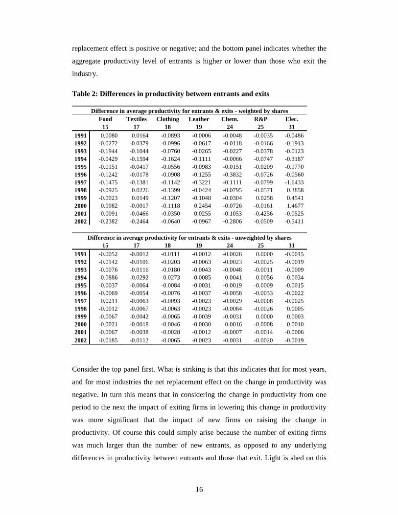
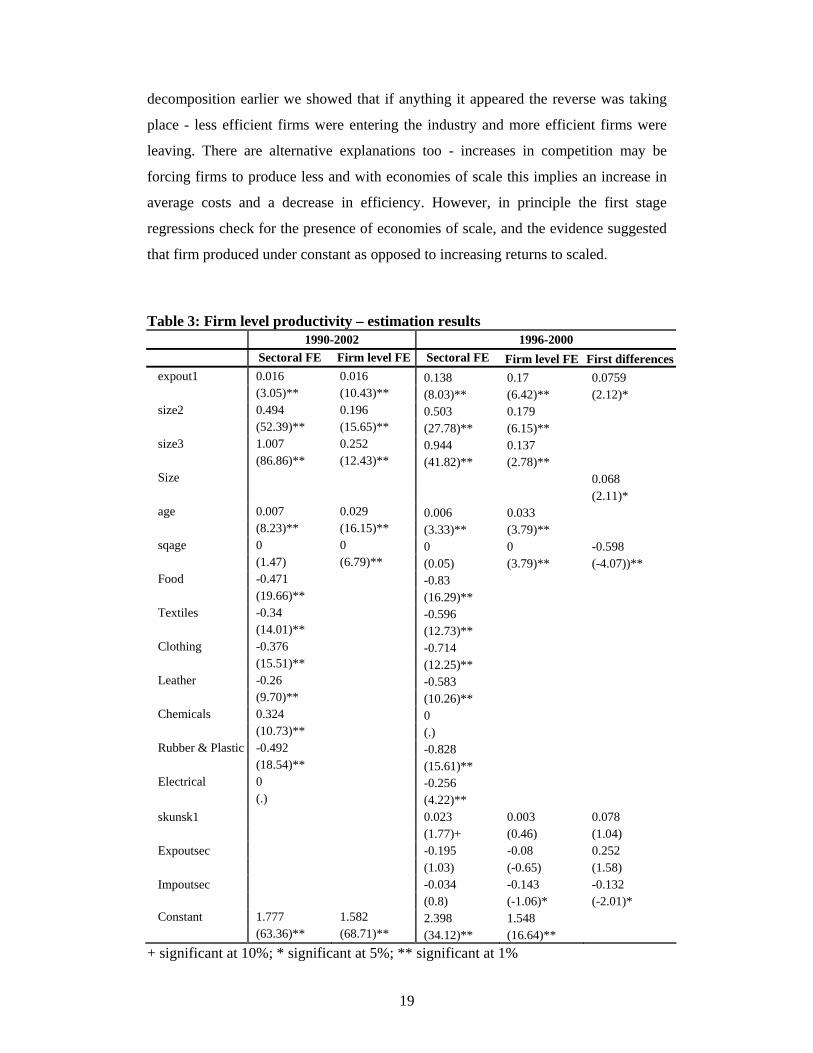
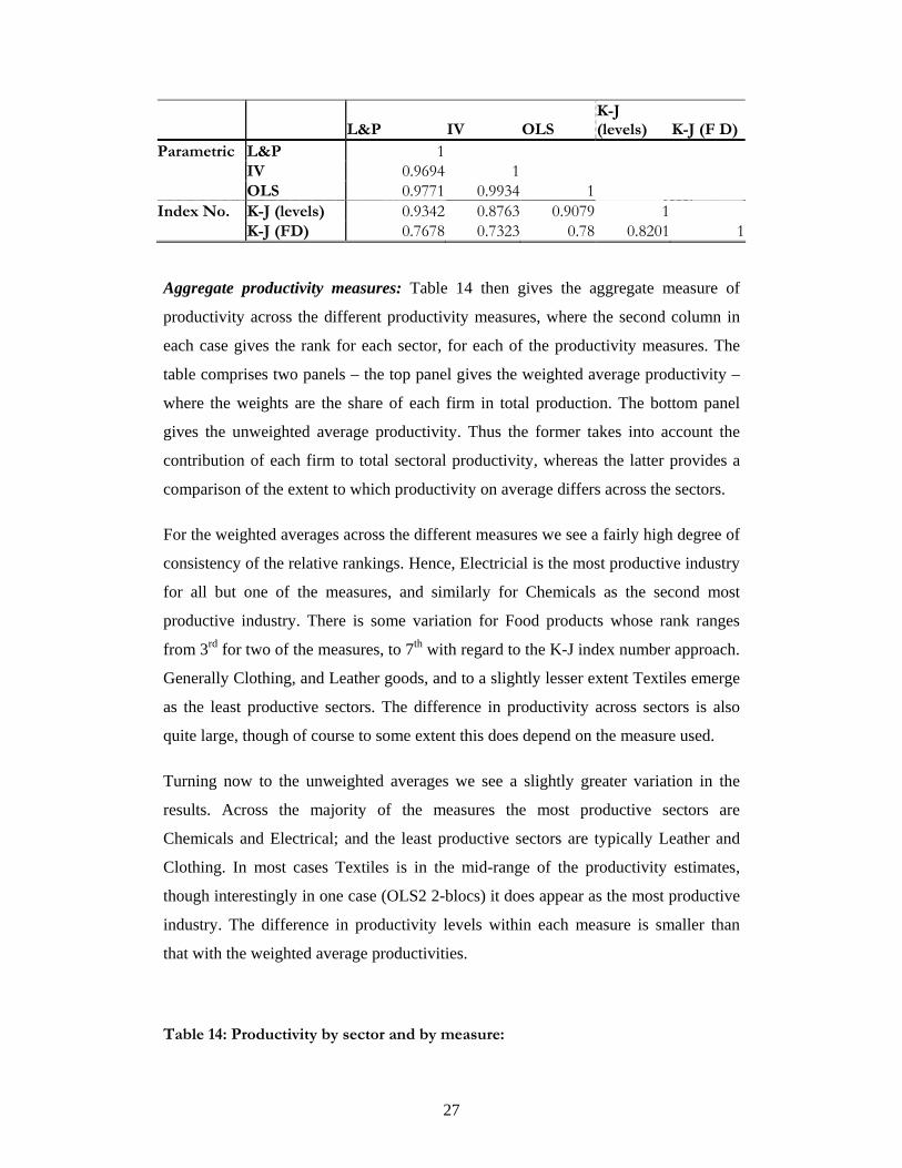
The first aspect worth noting is that there is no unambiguous relationship between
higher levels of productivity and exporting in this data. For example in Electricals
30
across all the measures of productivity it is the non-exporters which are more
productive. In contrast for Clothing, Plastics and Rubber, and Textiles it is the
exporters across all the productivity measures which are more productive. For the
remaining sectors the picture is more mixed and depends on the measure of
productivity employed. Finally it is interesting to compare the relative ranking across
the different categories of firms. Hence for non-exporters the most productive
industries are Chemicals and Electrical, and the least productive industries Leather,
Clothing, and Rubber and Plastic. In contrast for exporting firms the contribution to
aggregate weighted productivity is highest for Rubber and Plastics, followed largely
by Textiles and Chemicals.
4.3.2: The determinants of productivity - FACS
In the preceding we used descriptive statistical analysis to see what could be learnt
from the productivity estimates derived in the first stage of our methodology. In this
section of the paper we explore these relationships more formally, by econometrically
testing for the significance of some of these relationships. As before the purpose is in
order to try and better understand the possible determinants of productivity.
The underlying FACS survey is very rich in firm level detail. Hence the number of
possible explanatory variables is potentially quite considerable. In the first instance
we have focussed on those variables which a priori one might expect to be important.
Here we distinguish between those variables, which are related to international trade,
institutional variables, and those, which relate to firm specific characteristics such as
the age of the capital stock or information on R&D at the firm level. The results are
given in Table 9, where we give the results for the estimations based on the six
different productivity measures detailed earlier. In each case the model was run with
both sectoral and regional dummies but these are not reported here. The explanatory
variables we include here are:
1. Trade barrier variables:
31
Tariff barriers on exports Non-tariff barriers on exports Average domestic tariffs
2. Intermediate trade variables:
Share of imported intermediates Share of imported capital Share of imported raw materials Duty paid on imported capital
3. Other trade variables
Share of production exported (calculated at the firm level) Share of production exported (calculated at the sectoral level) Preparation undertaken for trade liberalisation with the EU.
4. R&D variables
Does the firm invest in R&D No of products less than 5 years old Share of workforce in R&D
5. Capital variables
Age of capital less then 5 years old Age of capital between 5 & 10 years old Age of capital more than 10 years old Training by suppliers (of new machinery) Training undertaken abroad Training from manuals
6. Other
Share of foreign ownership Has the firm experienced any infrastructure related difficulties in the
preceding year. Is the firm multiplant? Has the firm applied for MEDA funding Are the firm’s products ISO certified No. of employees.
In this first table of results we have included all the coefficients which a priori one
might consider could be important or could play a role in explaining differences in
productivity across firms. A number of these coefficients prove not to be statistically
significant. We include them here however, partly to indicate that this was indeed the
case, and partly because it is frequently worth reflecting on why this might arise. In
the second table, we then run the same regressions but this time on much smaller
sample of explanatory variables essentially largely on those which the first sets of
regressions suggested are statistically significant.
32
The first column of the table gives a brief description of the variable. Several of the
variables are dummy variables where the firm was, for example, asked to respond yes
or no; some of the variables are dummy variables, some of the variables are shares,
and some are absolute values. Hence if, for example, we take the second row of the
results where we report on whether firms perceived non-tariff barriers to trade to be
an obstacle in export markets. Those firms that do perceive there to be such an
obstacle, are ceteris paribus and on average 62% more productive, when the
estimation is based on the Klette-Johansen productivity measures. Where a variable is
a share or percentage, than the marginal effect is a semi-elasticity. It gives the
percentage impact on productivity as a result of one percentage point increase in the
variable. Finally, there are two variables in absolute values – the number of new
products, and the total no.of employees. These variables were logged and hence the
coefficient on the variable gives the elasticity.
If we now turn to the results. The first shaded panel of the table focuses on the trade
related variables. Here we look at variables with respect to both firms’ export markets
as well as the domestic market. With respect to the export market the firms report on
whether they experienced any difficulties in exporting either arising from high tariffs
or from non-tariff barriers in export markets. Here we might expect that high tariffs
impede exports and thus reduce the incentives for firms to improve productivity
levels. If this were true we might expect a negative coefficient on this variable.
However, it is equally possible that successful, exporting firms face higher barriers
precisely because they are more productive and thus more successful. In this case we
could find a positive coefficient. Interestingly the coefficient on tariff barriers is
significant and negative for three of the estimations and suggests that firms that
experience higher barriers in export markets are approximately 25% less productive.
In contrast the coefficient on non-tariff barriers is positive across all the models, and
significant in three cases. The size of the coefficient suggests that firms with
perceived non-tariff barrier obstacles to trade are on average between 61% and 78%
more productive. It is worth noting, however, that this applies to 10 firms in the
sample.
With respect to protection in the domestic market the variable here represents,
average domestic tariffs. Here we have computed the average tariff based on each
33
firm’s three principal products exported. Hence this measure captures the degree of
domestic protection for the firm’s principal products. High domestic protection could
again reduce the incentives for firms to improve their productivity, and if this were
the case we would expect a negative coefficient on this variable. Again, there could be
reverse-causality here whereby inefficient firms seek greater protection. The
coefficient here is negative and statistically significant in all cases. Hence, if we take
the coefficient arising from the OLS2 procedure this suggest that a 1% point increase
in tariff protection corresponds with a decrease in productivity by 0.39%. Overall the
impact of domestic tariffs on productivity is negative across all the regressions and
significant for all but one. The impact of a 1% increase in domestic tariff protection
on productivity ranges from 0.38-0.49%. There is clear evidence then that protected
domestic industries tend to be less productive.
Looking at the second bloc of results, the intermediate trade variables, we see that in
none of the cases are any of the variables statistically significant. The aim here was to
seek to establish whether there is any evidence if the presence of imported and
possibly higher quality intermediates might be related to higher productivity levels
(see for example Amiti, 2004). There appears to be little direct evidence of this here.
In the third panel of the table we examine other trade related variables. The first two
of these look at the relationship between exporting and productivity, as there is some
evidence in other studies that exporting firms tend to be more productive. There are
important issues of causality here, but the aim in the first instance is to investigate
whether such a relationship exists or not. The first of our variable here does so at the
level of the firm and the second at the sectoral level. At the firm level there is limited
evidence of a relationship between exports and productivity, and at the sectoral level
none of the coefficients are significant.
34
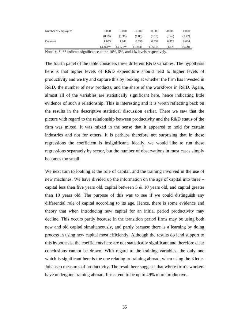
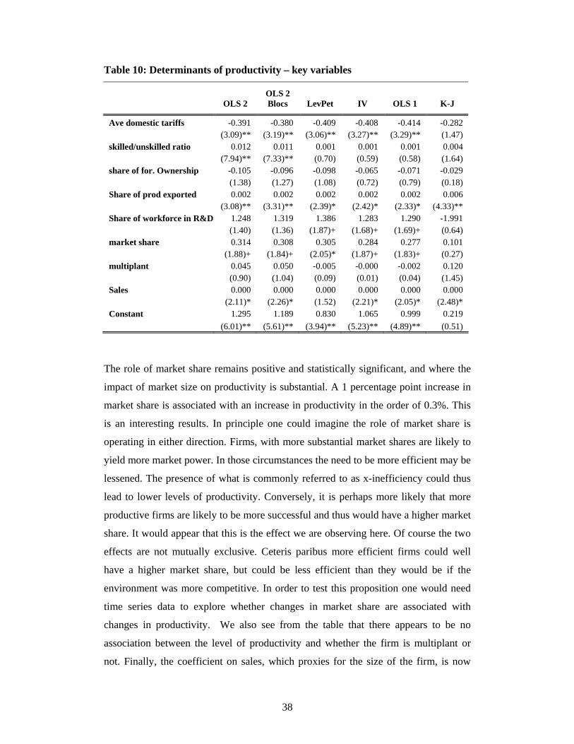
Table 9: Determinants of Productivity – cross section
OLS 2 OLS 2 Blocs LevPet IV OLS 1 K-J
Tariff obstacles on exports -0.138 -0.133 -0.242 -0.202 -0.209 0.040
(1.23) (1.17) (2.24)* (1.87)+ (1.93)+ (0.23)
NTB obstacles on exports 0.582 0.538 0.394 0.430 0.424 0.480
(2.39)* (2.20)* (1.50) (1.52) (1.50) (2.30)*
Ave domestic tariffs -0.392 -0.381 -0.478 -0.487 -0.492 -0.276
(2.87)** (2.95)** (3.41)** (3.69)** (3.70)** (1.30)
Share of imported interm. 0.003 0.003 0.002 0.002 0.002 0.002
(1.40) (1.47) (1.11) (1.20) (1.17) (0.89)
Share of imported raw mats -0.243 -0.230 -0.148 -0.131 -0.131 -0.202
(0.97) (0.97) (0.70) (0.63) (0.63) (0.72)
Share of imported capital -0.000 -0.000 -0.000 -0.000 -0.000 -0.001
(0.47) (0.43) (0.61) (0.35) (0.39) (0.81)
Share of prod exported 0.002 0.002 0.002 0.002 0.002 0.006
(2.61)** (2.77)** (2.44)* (2.01)* (2.02)* (4.21)**
Exp penetration (sector) -0.002 -0.002 -0.003 -0.003 -0.003 0.001
(0.34) (0.30) (0.38) (0.46) (0.45) (0.14)
Does the firm invest in RD 0.057 0.081 0.015 0.045 0.039 -0.165
(0.46) (0.64) (0.13) (0.39) (0.34) (0.55)
Number of new products -0.000 -0.000 -0.000 -0.000 -0.000 0.004
(0.19) (0.19) (0.28) (0.18) (0.19) (2.00)*
Share of workforce in R&D 0.996 1.002 1.492 1.256 1.284 -1.575
(1.19) (1.11) (2.02)* (1.80)+ (1.82)+ (0.49)
Age of capital < 5 years 0.094 0.050 0.024 0.284 0.278 -0.429
(0.56) (0.30) (0.16) (1.44) (1.41) (1.42)
Age of capital: 5-10 years 0.152 0.097 0.130 0.369 0.365 0.133
(0.93) (0.59) (0.85) (1.85)+ (1.83)+ (0.51)
Age of capital > 10 years 0.063 0.033 0.033 0.229 0.228 -0.182
(0.35) (0.18) (0.19) (1.04) (1.04) (0.53)
Training by suppliers 0.088 0.075 0.119 0.136 0.132 -0.181
(0.92) (0.78) (1.25) (1.44) (1.39) (0.57)
Training abroad 0.026 0.030 0.057 0.072 0.069 0.396
(0.22) (0.24) (0.50) (0.68) (0.64) (1.82)+
Training from manuals -0.106 -0.141 -0.016 -0.026 -0.028 -0.134
(0.85) (1.12) (0.14) (0.23) (0.24) (0.39)
Share of for. Ownership -0.109 -0.103 -0.200 -0.188 -0.191 -0.312
(1.18) (1.13) (2.20)* (2.13)* (2.16)* (1.53)
Infrastructure problems 0.000 0.000 -0.000 -0.000 -0.000 -0.003
(0.23) (0.08) (0.19) (0.67) (0.62) (1.82)+
market share 0.420 0.411 0.496 0.518 0.508 0.326
(2.41)* (2.34)* (3.21)** (3.24)** (3.17)** (0.82)
No. of competitors -0.000 -0.000 -0.000 -0.000 -0.000 -0.000
(1.52) (1.50) (0.70) (0.83) (0.82) (1.08)
multiplant firms -0.009 -0.008 -0.047 -0.036 -0.037 0.042
(0.23) (0.19) (1.35) (1.04) (1.07) (0.61)
Meda funding applied for 0.119 0.156 0.143 0.174 0.172 0.453
(1.03) (1.37) (1.36) (1.79)+ (1.75)+ (2.19)*
iso 0.106 0.082 0.100 0.140 0.130 0.413
(0.75) (0.57) (0.77) (1.08) (0.99) (2.26)*
35
Number of employees 0.000 0.000 -0.000 -0.000 -0.000 0.000
(0.59) (1.30) (1.06) (0.13) (0.46) (1.47)
Constant 1.053 1.041 0.556 0.534 0.477 0.004
(3.26)** (3.17)** (1.84)+ (1.65)+ (1.47) (0.00)
Note: +, *, ** indicate significance at the 10%, 5%, and 1% levels respectively.
The fourth panel of the table considers three different R&D variables. The hypothesis
here is that higher levels of R&D expenditure should lead to higher levels of
productivity and we try and capture this by looking at whether the firm has invested in
R&D, the number of new products, and the share of the workforce in R&D. Again,
almost all of the variables are statistically significant here, hence indicating little
evidence of such a relationship. This is interesting and it is worth reflecting back on
the results in the descriptive statistical discussion earlier. There we saw that the
picture with regard to the relationship between productivity and the R&D status of the
firm was mixed. It was mixed in the sense that it appeared to hold for certain
industries and not for others. It is perhaps therefore not surprising that in these
regressions the coefficient is insignificant. Ideally, we would like to run these
regressions separately by sector, but the number of observations in most cases simply
becomes too small.
We next turn to looking at the role of capital, and the training involved in the use of
new machines. We have divided up the information on the age of capital into three –
capital less then five years old, capital between 5 & 10 years old, and capital greater
than 10 years old. The purpose of this was to see if we could distinguish any
differential role of capital according to its age. Hence, there is some evidence and
theory that when introducing new capital for an initial period productivity may
decline. This occurs partly because in the transition period firms may be using both
new and old capital simultaneously, and partly because there is a learning by doing
process in using new capital most efficiently. Although the results do lend support to
this hypothesis, the coefficients here are not statistically significant and therefore clear
conclusions cannot be drawn. With regard to the training variables, the only one
which is significant here is the one relating to training abroad, when using the Klette-
Johansen measures of productivity. The result here suggests that where firm’s workers
have undergone training abroad, firms tend to be up to 49% more productive.
36
Finally, in the last panel of the table we explore the role of other firm specific
variables. The first of these focuses on the share of foreign ownership by firm. Here
we are interested in exploring whether high rates of foreign ownership lead to firms
being more productive, for example through the introduction of techniques and
technologies from abroad. If this were the case we would expect the coefficient here
to be positive. Interestingly the coefficient is negative and in several of the parametric
approaches statistically significant. This suggests that firms with a higher degree of
foreign ownership tend to be less productive. This is an interesting and possibly
counter-intuitive results.
For the second variable (infrastructure problems) firms reported on a number of
possible problems which may have impacted on their production in the preceding
year. These include electricity cuts, water shortages, days lost as a result of strikes or
disputes with workers etc. Here we have aggregated all these into a single dummy
whenever a firm has reported on the presence of such a problem in the preceding year.
Production problems such as these are likely to impact negatively on productivity, and
hence we would expect to find a negative coefficient. However, the coefficient is
negative and statistically significant only when using the Klette-Johansen measures,
and suggests that where firms did experience such difficulties on average firms were
0.3% less productive.
The following two variables deal with the extent of competitive interaction firms face.
The first of these gives each firm’s domestic market share, and the second of these
gives the number of competitors each firm perceives itself to have for its principal
product. There is evidence here that a higher domestic market share leads to higher
levels of productivity and this is true of all the parametric based results. The
coefficient is also positive for the Klette-Johansen index, but not statistically
significant. There little evidence that an increased number of competitors tends to
decrease productivity. In terms of the remaining variables two appear significant in
certain cases. For the first of these firms were asked whether they had applied for any
MEDA funding. Eleven firms replied in the affirmative, and these firms are on
average between 19% (OLS1) and 57% (Klette-Johansen) more productive, ceteris
paribus. Again, it is important to be careful with interpretation here, as there could be
reverse causality at work. Hence it is just as likely that it is the more productive firms
37
that apply for MEDA funding, as it is that MEDA funding helped to boost firms
productivity. In order to answer this question we would need panel data. Finally, we
also have information on whether the firm’s products are ISO certified or not. Using
the Klette-Johansen measure it appears that ISO certified firms tend to be on average
51% more productive. This is an interesting result, which could have several
interpretations. One possible interpretation is that ISO certification itself cannot lead
to higher productivity, and therefore this is simply a reflection of that in order to be
ISO certified firms are required to produce higher quality goods and therefore in order
to do so (competitively) they need to be more productive. This in turn however raises
questions about the motives and processes underlying the ISO certification process.
Alternatively it is possible that ISO certification because it provides a guaranteed
mark of quality allows firms to charge higher prices, and this is being picked up by
our productivity measures. Finally the last row of the table gives the number of
employees which can be seen as a proxy for size. There appears to be no evidence that
larger firms are more productive, and therefore no evidence of economies of scale.
Given the lack of significance of a number of the preceding variables, in the next table
we turn to a similar set of estimations but this time run on a reduced set of
explanatory variables. The first row of the Table 10, thus gives the significance of the
extent of average domestic tariffs. Once again this clearly indicates that domestic
tariff protection is negatively correlated with productivity levels where a 1% increase
in domestic tariffs is associated with approximately a 0.4% decrease in productivity.
In the second row we include the ratio of skilled to unskilled workers for each firm.
Here we are interested in exploring whether there is any evidence that firms, which
employ a higher proportion of skilled workers may be more or less productive. The
coefficient here is positive, hence indicating that the greater the skill intensity the
higher the productivity, but is only statistically significant for two of the productivity
measures (OLS2 and OLS2 Blocs). Once again the share of foreign ownership is
negatively related to productivity, although the coefficients remain statistically
insignificant. Productivity is also positively related to the share of production
exported at the firm level, as well as the share of the workforce involved in R&D
activity. There is a negative coefficient with regard to this latter variable for the
Klette-Johansen measure of productivity but this is not statistically significant.
38
Table 10: Determinants of productivity – key variables
OLS 2 OLS 2 Blocs LevPet IV OLS 1 K-J
Ave domestic tariffs -0.391 -0.380 -0.409 -0.408 -0.414 -0.282 (3.09)** (3.19)** (3.06)** (3.27)** (3.29)** (1.47) skilled/unskilled ratio 0.012 0.011 0.001 0.001 0.001 0.004 (7.94)** (7.33)** (0.70) (0.59) (0.58) (1.64) share of for. Ownership -0.105 -0.096 -0.098 -0.065 -0.071 -0.029 (1.38) (1.27) (1.08) (0.72) (0.79) (0.18) Share of prod exported 0.002 0.002 0.002 0.002 0.002 0.006 (3.08)** (3.31)** (2.39)* (2.42)* (2.33)* (4.33)** Share of workforce in R&D 1.248 1.319 1.386 1.283 1.290 -1.991 (1.40) (1.36) (1.87)+ (1.68)+ (1.69)+ (0.64) market share 0.314 0.308 0.305 0.284 0.277 0.101 (1.88)+ (1.84)+ (2.05)* (1.87)+ (1.83)+ (0.27) multiplant 0.045 0.050 -0.005 -0.000 -0.002 0.120 (0.90) (1.04) (0.09) (0.01) (0.04) (1.45) Sales 0.000 0.000 0.000 0.000 0.000 0.000 (2.11)* (2.26)* (1.52) (2.21)* (2.05)* (2.48)* Constant 1.295 1.189 0.830 1.065 0.999 0.219 (6.01)** (5.61)** (3.94)** (5.23)** (4.89)** (0.51)
The role of market share remains positive and statistically significant, and where the
impact of market size on productivity is substantial. A 1 percentage point increase in
market share is associated with an increase in productivity in the order of 0.3%. This
is an interesting results. In principle one could imagine the role of market share is
operating in either direction. Firms, with more substantial market shares are likely to
yield more market power. In those circumstances the need to be more efficient may be
lessened. The presence of what is commonly referred to as x-inefficiency could thus
lead to lower levels of productivity. Conversely, it is perhaps more likely that more
productive firms are likely to be more successful and thus would have a higher market
share. It would appear that this is the effect we are observing here. Of course the two
effects are not mutually exclusive. Ceteris paribus more efficient firms could well
have a higher market share, but could be less efficient than they would be if the
environment was more competitive. In order to test this proposition one would need
time series data to explore whether changes in market share are associated with
changes in productivity. We also see from the table that there appears to be no
association between the level of productivity and whether the firm is multiplant or
not. Finally, the coefficient on sales, which proxies for the size of the firm, is now
39
positive and statistically significant but the overall size of the coefficient is extremely
small.
There are a number of conclusions, which emerge from this section of the report.
First, we have explored the use of different approaches to measuring productivity.
Those different approaches each yield highly comparable and consistent results.
Secondly, our results suggest that the seven sectors covered in this data set all produce
under constant returns to scale, and except for food have similar capital-labour ratios.
We then explored the possible determinants of productivity, though bearing in mind
the issue of reverse causality, which is present with respect to a number of our
variables. The key results indicate that more productive firms tend to face lower
domestic tariffs, export more, have a larger domestic market share, and have a higher
proportion of workers engaged in R&D activity. It also appears to be the case that
firms which are more productive may have applied for MEDA funding, and may have
products which are ISO certifies. In contrast there appears to be little evidence to
suggest that imported intermediates, training in the use of equipment, foreign
ownership or size appear significant determinants of productivity. All these are factors
that a priori one might expect to influence the level of productivity.
4.3: Egypt
The data for Egypt derives from the CAPMAS industrial survey (1983-1994) and
gives information at the sectoral as opposed to firm level. Within each sector however
there is a distinction between public sector firms, and private sector firms, and within
each of these there is information by size class of firms. In total there are nine sectors
in the survey and these are: Food, Beverages and Tobacco (FBT), Textiles, Clothing
and Leather (TCL), Paper products, Chemical products, Wood products, Non-metallic
minerals, Base Metals, Metal products, and Other manufacturing.
In the case of Egypt the size and role of the public sector is extremely important,
hence the need to distinguish between the two. At the beginning of the period the
share of the public sector was very high in a number of sectors such as Wood
Products (over 90%), and Food, Beverages and Tobacco, and Textiles, Clothing and
Leather (just under 80%). The sector with the smallest public sector involvement was
40
Other (just over 20%), followed by Paper (~40%) and Chemicals (~45%). By the end
of the period the sector with the largest public sector share was Non-metallic Minerals
(just over 75%), followed by Food, Beverages and Tobacco, and Basic Metals
(around 60%). The share of the public sector declined significantly for all sectors over
the period.
4.3.1 Analysing the productivity estimates
Figure 5 gives the aggregate change in productivity over the period in question –
1983-1994. As in the previous discussion of Morocco these measures of productivity
over time are derived from production function estimatations, and the full
methodological details can be found in Appendix 3. Whereas for Morocco this was
based on firm level data, here the estimations are based on sectoral data, but where
within each sector we distinguish between both the public and the private sector, and
where we distinguish between different size classes. We thus report on two measures
of aggregate productivity here - productivity over time for both the public and the
private sector, where the weights in the aggregation procedure are given by the shares
in production.
Figure 5: Aggregate TFP over time: Public and Private sector
00.5
11.5
22.5
33.5
44.5
5
1983
1984
1985
1986
1987
1988
1989
1990
1991
1992
1993
1994
Year
TFP Public
Private
A number of interesting features emerge from the Figure. First, it is noticeable that the
private sector has consistently much higher productivity than the public sector and
this is true over the entire time period. Secondly both sectors experience a rise in
41
productivity over the entire time period (except for one anomalous year for the private
sector). That increase is just under 42% for the private sector, and 49% for the public
sector. However, in the latter part of the period, from 1990 onwards, while the private
sector experiences productivity growth of over 20%, the public sector witnesses a
decline in productivity.
4.3.2: Econometric Analysis
We now turn to the second stage of our analysis. Here we take the productivity
estimates for both the public and the private sector, for each of the ISIC industries and
for each of the size classes, and run several regressions in order to establish the
possible significance of key explanatory variables. In comparison to the Moroccan
case we have significantly less information with regard to the explanatory variable.
Here, therefore, we focus on the role of openness, and on the role of firm size. With
regard to openness, as earlier we capture this with the two variables exports/output
and imports/output in each case at the sectoral level. Tariff data is unfortunately not
available for the relevant years. With regard to size, as above, we have six size classes
of firms by numbers of employees – less than 10, 10-25 employees, 25-50
employeees, 50-100 employees, 100-150 employees, and greater than 500 employees.
The regressions are then run separately on the public sector and on the private sector,
and in each case we also run the model both with and without sectoral fixed effects.
Hence the first two columns of the Table 11 give the results for the public and the
private sector, but with no sectoral fixed effects. There are some striking features
which emerge from these results. First, none of the coefficients for the public sector
are significant – which suggests that in this data there is no evidence that changes in
exports behaviour, openness of the domestic market, or the size of the firm play any
significant role in determining productivity. This is interesting and to a large extent
corroborates the picture, which emerged earlier concerning the diverse changes in
productivity over time in the public sector, and the lack of a correlation between
productivity levels and size class.
Table 8: Determinants of productivity - Egypt
42
Variable Public Private Public Private
Impoutsec 0.021641 -0.13471 0.047417 -0.12386 (0.76) (-3.65**) (0.98) (-1.82+)
Expoutsec -0.18833 0.889801 -0.33111 1.607784 (-0.65) (1.6) (-0.69) (2.11*)
size1 (less than 10) 0.1139 -1.59989 0.283249 -1.65836 (0.52) (-5.68**) (1.19) (-5.93**)
size2 (10-25) 0.192999 -0.41958 0.210601 -0.35488 (1.34) (-3.12**) (1.5) (-2.73**)
size3 (25-50) 0.114318 -0.72949 0.089258 -0.67763 (0.71) (-4.75**) (0.65) (-4.45**)
size4 (50-100) 0.061867 -0.56188 0.048112 -0.49714 (0.51) (-3.97**) (0.44) (-3.61**)
size5 (100-500) -0.40291 -0.04999 -0.38571 -0.00737 (-4.16) (-0.37) (-3.94**) (-0.06)
sector 32 0.15454 -0.58086 (0.62) (-2.77**)
sector 33 0.159013 -0.69979 (0.82) (-3.01**)
sector 34 0.16715 -0.53202 (1.2) (-2.54*)
sector 35 1.414068 -0.07635 (8.65**) (-0.38)
sector 36 -0.08255 -0.21851 (-0.49) (-1.07)
sector 37 0.04548 -0.9883 (0.22) (-4.26**)
sector 38 -0.05939 -0.00681 (-0.45) (-0.03)
sector 39 -0.03235 -0.94468 (-0.11) (-4.68**)
_cons 0.789866 3.293628 0.558545 3.613052 (15.24**) (29.17**) (5.08**) (18.12**)
Absolute value of t statistic in parentheses + significant at 10%; * significant at 5%; ** significant at 1%
If we now turn to the private sector a different picture emerges. The first row indicates
that increases in domestic openness, captured here by imports/output, serve to
decrease productivity levels. The size of the coefficient suggests that a 10% increase
in this variable, decreases productivity by 1.3%. The coefficient on exports/output is
positive but not statistically significant. Secondly, each of the size coefficients except
for one are negative and highly statistically significant. These coefficients should be
interpreted as being in comparison to the largest size class (greater than 500
employees). Hence the results indicate that relative to this largest size class, each of
the other size class have a lower productivity. As before these are dummy variables
therefore the size of the effect can be found by taking [exp(dummy)-1]*100. Applying
43
this we see that the results suggest that firms with 50-100 employees are 43% less
productive, and small firms (less than 10 employees) are 80% less productive, on
average and ceteris paribus. There is no evidence that firms with between 100-500
employees are more or less efficient than those with more than 500 employees.
If we now consider the last two columns of the table, here we report on the results
when we allow for sectoral dummies. Thus here we are controlling for any possible
differences that may arise due to factors common to any given sector. Once again the
results for the public sector are almost invariable insignificant. There is some
evidence that firms with 100-500 employees are less productive than larger firms, and
there is some evidence that sector 35 (non-metallic minerals) is relatively more
productive. For the private sector, the results are similar to those in the earlier
experiment. For example we see the same pattern of results with regard to the size
classes of firms.
We also see that once again increased imports/output serves to decrease productivity.
We also saw some evidence of this when looking at the results for Morocco. Whereas
in the earlier regression the variable exports/output was not statistically significant,
now it is significant and the coefficient is positive. This too reinforces the results we
saw when looking at the Moroccan data, which is that there is a positive relationship
between increases in exports and increases in productivity. The size of the coefficient
is quite large suggesting that a 10% increase in export/output is associated with a 16%
increase in productivity, on average and ceteris paribus. We also ran the regressions
separately on each size class of firms (not reported here). There we found a positive
correlation between firm size, productivity and exporting activity. Hence, an increase
in exports/output leads to the following changes in productivity: less than 10
employees: 11.8%; 10-25 employees: 30%; 25-50 employees: 14.4%; 50-100
employees: 14.6%; 100-500 emplyees: 21.6%; more than 500 employees: 40.9%.
Finally, we see that four of the sectoral dummies (textiles, clothing and leather, paper
products, non-metallic minerals, and wood products) are negative and statistically
signficant – this indicates that relative to the omitted sector (food, beverages and
tobacco), these sectors have a lower productivity.
In summary the picture that emerges for Egypt is both complicated and interesting.
The complications arise from the important differences between the private and the
44
public sector. As seen earlier the public sector over the time period in question
comprised an important (though declining) proportion of manufacturing in Egypt.
Productivity in this sector was consistently lower, and more variable than productivity
in the private sector. There is little evidence of much of a pattern either at the industry
level, or at the level of the size class of firms. There is also no apparent relationship
between increases in trade openness, either with regard to imports or with regard to
exports, and levels of productivity. The picture is then quite different with regard to
the private sector. Here we see much higher levels of productivity, consistent
differences in productivity across sectors, and significant coefficients with regard to
size, and trade openness. The evidence suggests that (a) larger firms are more
productive than smaller firms, (b) that increased access to export markets (as a
proportion of domestic output) is positively associated with levels of productivity, and
(c) that increased imports tend to lower levels of productivity.
45
5. Summary and policy implications:
1. The decomposition of the sources of productivity growth over time for Morocco
indicated that in aggregate the contribution of changes in firm level productivity to
aggregate productivity was small, and appeared to be declining over time. Thus
the evidence appears to suggest that changes in firm level productivity were
relatively modest, and this was true of most sectors.. Our results also appeared to
suggest little evidence of economies of scale which could enable productivity
improvement to occur via scale effects. It would be interesting to examine more
carefully the issue of the presence of lack of economies of scale and to see if there
are factors specific to the economic environment which mitigate against the
exploitation of economies of scale. In addition to the above, and reinforcing the
message from the discussion earlier, it is important not to underestimate the
importance of the overall environment and the presence of appropriate flanking
policies which enable firms to increase the productivity and competitiveness. This
touches upon issues such as the quality of service provision, the competitiveness
and flexibility of the financial sector, administrative and bureaucratic procedures,
infrastructure investment and so on. An improved economic environment, and
improved flexibility in product and factor markets, can greatly facilitate
productivity improvement.
2. To the extent then that changes in productivity are driven more by sectoral
reallocation effects and by the entry and exit of firms, this also suggests
considerable churning in the labour market. This is reinforced when we look at the
proportion of new firms and exiting firm in any given year as a proportion of the
total number of firms for that year. On average over 1990-2002 the proportion of
exiting firms was 10.4%, and the proportion of new firms 9.5%. This is a high
figure, which indicates considerable turnover amongst firms, and consequently in
the labour market1. There is clearly then a need for policies, such as social security
1 It is of course possible and likely that to some extent these figures overstate the extent of entry and exit of firms. Although the data is based on a census it is clearly possible and likely that firms simply may not report in any given year, and thus appear as exiters, and then choose to report in a subsequent year and then would appear as entrants. To some extent we have attempted to control for this. Hence,in the data where a firm disappears from the data set, but the reappears either a year or two years later, we
46
policies, designed to alleviate the short term adjustment costs associated with
these processes. There is also a need for policy to assess why there appears to be
such a high-degree of firm level turnover. This would involve examining in more
detail the characteristics of the entrants and exiters, and seeking to establish
whether for example exiting firms are genuinely exiting because of a lack of
competitiveness of due to other reasons.
3. There is some evidence in our analysis for Morocco that changes in the skill-
composition of the workforce at the firm level impacts positively upon
productivity – however the evidence is slight. This in turn might suggest that
change in policy at the firm level designed to increase productivity, or the entry
and exit of firms does not appear to be significantly impacting upon the skill
composition of the workforce and hence on factor returns. Care, however, should
be taken in drawing this conclusion, as the division of workers by skill category
may well differ across industries and thus might be impacting upon our results.
4. In contrast what is clear both from our analysis of Morocco and of Egypt is that
there are important changes in the sectoral shares in production (for example the
growing share of clothing and electrical in Morocco, the changes between the
private and the public sector for Egypt) which again point to structural adjustment
and the need for policies to alleviate that process of adjustment both at the level of
the individual but also at the level of the firm. What is interesting is that these
processes are not clearly linked to changes in productivity at the sectoral level,
and this again is related to the discussion above concerning the high rates of entry
and exit.
5. There is clear evidence that trade and openness do interact in important ways with
productivity. Here we need to distinguish between openness at the level of
exports, and openness at the level of domestic imports:
Export openness: The results suggest that exporting activity tends to lead to higher
levels of productivity, and not surprisingly the extent of that impact differs across
sectors, but also across different size classes of firms. One has to bear in mind that
have interpolated the missing data, and thus the firm is then treated as being an incumbent throughout the time period.
47
there is an issue of endogeneity here in that it could be that higher levels of
productivity may lead to higher export levels, as opposed to higher export levels
leading to higher productivity. However, the nature of the fixed effects regression,
as well as the analysis in first differences lends more support to the latter.
There is then a clear need to understand more fully what drives this association
between exporting and productivity, and the source of the variation in this
relationship across sectors. Some of the difference in the productivity of those
firms that export and those that do not may arise from differences in the other
characteristics of these firms. An appropriate methodology for exploring this is
based on the Oaxaca decomposition. The principle underlying the Oaxaca
decomposition is that the sample is divided into two groups (in this case exporting
firms and non-exporting firms), and then the regression of productivity on the
explanatory variables is run separately on each of the two sub-groups. The
decomposition then considers the source of the difference between the
productivity levels across the two groups. Hence, it is possible that the difference
in productivity levels is entirely explained by these other characteristics. For
example, it is possible that exporting firms, are also larger firms, and that the
difference in productivity is entirely explained by this difference in size.
Similarly, with respect to the age of the firm. This aspect of the difference in
productivity is called the “difference in characteristics”. Alternatively it is
possible, that all these other characteristics do not explain any of the difference in
productivity, but instead that the exporting firms derive a higher productivity out
of their given characteristics. For example that for a firms of a given size and age
etc, that the exporting firms have a higher return (productivity) on those same
characteristics. This aspect of the decomposition is know as the “difference in
returns”.
Given the importance of the relationship between exports and productivity we
have then run the Oaxaca decomposition for our Moroccan sample of firms over
the period 1996-2002. That decomposition suggests that 42% of the difference in
productivity between exporting and non-exporting firms derives from the
difference in characteristics, and that 58% of the difference derives from the
difference in returns. This is extremely interesting, for it suggest that in part it is
48
the difference in the characteristics in the firms that matters – and from the
aggregate estimations this is likely to be associated with size and age of firms. But
importantly we see that an important part of the difference arises from the
differences in the returns to those characteristics for the exporting firms. This
raises interesting questions as to whether this arises as a result of greater exposure
to technology or market conditions in export markets, or does this arise from a
need to produce to certain standards (imposed either at the level of eg. the EU, or
by individual subcontracting firms.).
In terms of policy, it is important that policy focuses on ensuring the appropriate
environment for firms to engage in exporting activity. Recognising that
productivity and exporting status are positively correlated should not lead to a
return to simple export promotion policies, nor to a policy of trying to pick future
export growth firms or industries. More important is to ensure that the correct
environment is in place. This involves a focus on issues such as infrastructure, the
bureaucratic arrangements in place, customs procedures, the regulatory and
institutional environment for exporters, as well as costs of transport. Thus policies
aimed at improving local infrastructure, aimed at better understanding the
regulatory and /or bureaucratic obstacles or barriers to exporting are all likely to
improve that environment, encourage a higher growth of exports and thence
productivity, and ultimately poverty. The preceding focussed on the domestic
market, but equally it is important that policy addresses issues of access to export
markets. Those issues of access clearly concern both direct barriers to trade such
as remaining tariffs or quotas, as well as indirect barriers to trade such as the role
of rules of origin in constraining firms’ access to markets. Reducing such barriers,
reducing protection of key competing European industries, simplifying and
relaxing the rules of origin are all important policies to be pursued.
Access to market also concerns issues of what is often referred to as “deep
integration”. Here one typically has mind issues of quality assurance, norms and
standards, after sales service activities and links to distributors, knowledge of the
market and market research, developing links with commercial partners and so on.
These are issues both of information, but also of service provision. This too is an
area where policy makers can assist exporting or potential exporting firms. It is
49
also an area where it is important to ensure that norms and technical standards are
not being used as protectionist instruments but are instead there to facilitate
market access, and that the appropriate environment is in place for firms in order
to take advantage of that market access.
Import openness: Our results suggest mixed evidence on the impact of increased
domestic openness on productivity. For Morocco, in the time series analysis we
saw that increased openness in aggregate was negatively associated with
productivity. When we distinguished between small and large firms however, this
appeared to apply to the small firms and for the large firms there was a positive
relationship. For Egypt, where we only have aggregate results there is again a
negative coefficient. In contrast, for the Moroccan cross-section analysis (1998-
1999), we saw a negative coefficient on the average level of domestic protection.
This indicates that a reduction in domestic tariffs is associated with an increase in
productivity.
In the literature much has been made over a number of years of the supposed
benefits of the “cold shower of competition”. The increased domestic competitive
environment is supposed to lead both to the exit of less efficient firms, as well as
to increases in productivity (through for example reductions in x-inefficiency of
existing firms). What is interesting about our results here is that it is far from clear
that this is indeed occurring when looking at Egypt and Morocco. The picture that
emerges from the above is mixed, and the evidence suggests that both effects are
likely to be present. There are several possible explanations for this. One possible
explanation for the negative effect of increased openness on productivity is that
we are simply picking up on a short term phenomenon here, which is that the
heightened domestic competition is resulting in firms reducing their levels of
output. If firms produce under conditions of economies of scale that this reduction
in output increases average costs and thus decreases efficiency. Clearly, this may
well be the case, and it is thus more likely to apply to larger firms. However, it is
worth noting that in our regressions we tested for the presence of economies of
scale, and these were typically rejected. This therefore suggests, that maybe
alternative explanations need to be found. Those alternative explanations involve
50
looking more closely at understanding the mechanisms driving the changes in
aggregate productivity which we find.
Note that in order for a positive impact from the “cold shower of competition” it is
important that the correct domestic conditions have to be in place in order to allow
firms to adjust appropriately. Central here of course is the way that firms adjust to
changes in policy and ensuring that these adjustments are as optimal as possible.
From a policy point of view it is therefore important to understand more about the
causes of the exit of firms. Clearly if this occurs because of the increase in
competition and the lack of competitiveness of the firm than this constitutes part
of the necessary process of adjustment and change. However, if it occurs because
of, for example, limited and inefficient access to credit, or because of other
administrative and regulatory obstacles to productive activity than policy should
address those obstacles. Hence, an alternative explanation for the negative impact
of openness on productivity suggests that in the face of openness relatively
productive and possibly competitive firms may be exiting the industry because of
other constraints and difficulties.
Consider also that our results suggest that this negative coefficient appears to
impact more on the smaller firms. It is quite plausible to suppose that small firms
may indeed experience problems of invoices being paid on time, may have more
limited access to credit, or may be less able to deal with regulatory or
inftrastructure problems, or find it more difficult to meet the (growing) demands
made upon them by the firms with whom they have sub-contracted. It is also
plausible that changes in policy such as the Barcelona process invoke uncertainty
for firms. In the fact of uncertainty firms may well choose to invest less – either in
capital equipment, training of workers or R&D – which then impacts upon
productivity. Again, it is perhaps more likely that small firms would react
differently in the face of uncertainty than large firms. Hence there is a need to
understand better the constraints and needs of firms and in particular smaller
firms, and for policy to address those needs and concerns where it can.
On this issue it is finally also worth noting that it is also possible that small firms
may well resort to the informal sector faced with the need to adjust to changes in
policy. Hence, while for the purposes of our data they exit the industry, it might be
51
that instead they are producing in the informal sector. More generally, it is worth
emphasising that our analysis focuses on the data which is available and this
concerns the formal sector. The non-agricuiltural informal sector in Morocco, for
example, is very large and is estimated to constitute 17% of economic activity,
and 20% of total employment2. There is thus a clear need for policy to understand
better the relationship between the formal and the informal sector.
6. From the descriptive statistical discussion of the productivity estimates for Morocco
and Egypt there was some key sectoral patterns which emerged. These include
differential changes in productivity across sectors with certain sectors experiencing
large and positive changes in productivity while other sectors witnessed a decline. For
example in Morocco, Textiles, Chemicals, and Leather saw a decline in productivity
over the period. Similarly for Egypt there was a marked difference in the changes in
productivity between the private and the public sector, and then for individual
industries within these sectors. Changes in productivity are likely to be closely linked
to changes in competitiveness, and thus ultimately to sectoral changes in production.
Hence, prima facie, the results here shed light on sectors which may well have
experienced, be experiencing or are likely to experience problems with regard to
structural adjustment. These are thus sectors which thus may require more assistance,
or indeed different types of assistance than sectors where productivity and market
share appear to be growing.
Take textiles in Morocco as an example. This is a sector with low levels of
productivity growth, a declining share in production, and a rise in imports. In the
first instance therefore it would appear that this is a sector where policy could be
targeted in order to focus on the workers and firms being displaced as part of this
process. However, policy should not only be addressed to ease the process of
transition. It is also important to understand why these changes are taking place. Is it
the case that textiles in Morocco are uncompetitive and given the world market
conditions are likely to remain so? Alternatively, is their scope for increasing the
competitiveness of the sector. For example, are rules of origin sufficiently
constraining in the sector that this is impacting negatively on their competitivness,
and that signing regional trade agreements with other southern partners such as
2 “Synthese des principaux resultats de l’enquete nationale sur le secteur informel non-agricole” (1999/2000), Direction de la Statistique, Royaume du Maroc.
52
Turkey or Egypt which allow for diagonal cumulation could significantly impact on
their competitivness; is there scope for increasing the competitiveness in certain
aspect or niches in the textile market, and to what extent can facilitating sub-
contracting ease this process. These are difficult and important questions, but ones
which effective policy needs to address.
7. Another result which emerges from the preceding analysis is that there are
important differences in productivity levels, and in productivity changes by sector
and by size class. In part these issues were discussed in more detail above, when
we discussed the role of openness on productivity. The diverse relationship
between size class of firms and productivity highlights the importance of
recognising the heterogeneity of firms in both analysing productivity and
structural change but also with respect to policy.
8. As when discussing the issue of the difference in productivity between exporting
and non-exporting firms, it is important to establish the extent to which difference
in productivity by size class are driven by differences in other characteristics, or
by differences in the returns to those characteristics. For example, it may be that
larger firms are more productive because this reflects economies of scale (size),
but it may also be that there returns to scale are very low and there are other
constraints and issues which need to be addressed. In order to address these sort
of issues we employ the Oaxaca decomposition again, where look at the
difference in TFP between small and large firms for Morocco. Here we find that
26% of the difference in productivity appears to be explained by underlying
differences in other characteristics of small and large firms; and that 76% of the
difference is driven by the difference in returns from those characteristics. It is
clear that firms of different sizes appear to respond differently to changes in the
economic environment, and in particular that large firms obtain a higher return
from the same characteristics than do small firms.
53
Appendix: Approaches to Productivity Measurement The first stage of the empirical methodology requires estimating or calculating a measure
of productivity at the firm level. There are three principal techniques which are most
often utilised in the literature. These are parametrically estimating a production function
(eg. Cobb-Douglas or Translog), the index number approach, and Data Envelopement
Analysis (DEA). In this paper we work with both the parametric approach, as well as the
index number approach. The advantage of the latter concerns the ease of
implementation, allowing for technology to vary across individual units, as well as being
able to handle multiple outputs and inputs. The advantage of the former is that it is less
prone to measurement error and generated statistical tests for the significance of the
results. The principal underlying data required for each of these approaches is: value
added, variables to capture the cost of labour and the stock of capital. Value added is
calculated as the difference between total production and intermediate consumption. The
variables proxying for capital and labour respectively are the capital stock (machines and
buildings after depreciation) as reported in the balance sheet of the firms. and total
wages and social charges. With regard to the latter we do not have data on labour
disaggregated by type, hence using total wages and social charges we are capturing the
heterogeneity in labour that would not captured by using total hours worked or total
workers.
2.2.1 Parametric approaches
For the parametric approach we assume a standard neo-classical production function Qt=
Q(Lt, Kt), which we assume to be log-linear Cobb-Douglas:
Qt = α0 + αlLt + αkKt + ut (1)
Where α1 and α2 represent the Cobb-Douglas coefficients for labour (L), and capital (K)
respectively and ut is the error term. An OLS estimator could then be used to obtain a
fitted vector of coefficients α, and where then the residual captures productivity.
However, as is now widely recognised firms’ choice of inputs will depend on their
technology and productivity, which is in turn unobserved (Marschak & Andrews, 1944).
For example, more productive plants are more likely to invest more due to higher
54
productivity. The rationale for the relationship between productivity and the choice of
inputs can also be seen in the face of a positive productivity shock. For a profit
maximising firm a positive productivity shock raises the marginal product of capital and
labour, and with constant factor prices, the firm will expand output and hence use more
inputs to drive down the marginal products. Analogously for a negative productivity
shock. As productivity is unobserved and as the choice of inputs is likely to be correlated
with the former, the residual, which contains productivity will be thus be correlated with
L and K. This problem of simultaneity means that an OLS regression is likely to lead
biased estimates of the coefficients on capital and labour, and thus biased estimates of
productivity. In particular one would expect that the OLS regression would lead to an
upward bias in the capital coefficient and therefore maybe a downward bias in the labour
coefficient. In order to overcome this problem of simultaneity we use two alternative
methodologies. The first is that of instrumental variables, and the second follows the
semi-parametric approach of Levinsohn & Petrin (1999), which is in turn based on the
work of Olley and Pakes (1996). In both the IV and the OLS regressions we control for
sectoral and regional differences through sector and region-specific dummy variables.
For the IV estimation the instruments we use for capital and labour are lagged values of
capital (1998) and wages (1998) as well as the replacement book value of machines and
buildings (1999). We test for both the relevance and the validity of the instruments. For
the former we look at the R2 of the first stage regressions, and the results invariably
suggested the relevance of the instruments as the R2 with respect to the instrumented
regressors was typically over 0.9. For the latter we test that the instruments are
orthogonal to the errors using the Sargan and Basmann tests. Again across several
variants of the model the Sargan and Basman tests were invariably passed. As the use of
IV estimation to address the endogeneity problem implies a cost in terms of efficiency
vis-à-vis OLS, once the relevance and validity of the instruments is established, we then
use the Hausman test to see if there are systematic differences between the OLS and IV
estimates and thus whether the IV estimator is preferred to the OLS. Generally but,
interestingly, not invariably, it was the case that the IV estimation procedure was
preferred to the OLS procedure and that the OLS procedure tends to understate the
labour coefficient, and overstate the capital coefficient. This in line with our expectation
about the possible bias present in the OLS regression. We also tested for the presence of
constant returns scale and in no case was this rejected.
55
One of the implications, and possible limitations, of the parametric approach we utilise,
is that it imposes the same capital and labour coefficients across all sectors. In the cross
section regressions we tested for the valiidity of this by running the above procedure
with the inclusion of interaction terms between the sector specific dummies and capital
and labour, as well as running the regressions separately for each industry. Note that this
strategy reduces the number of observations available for the estimation of the sector
specific parameters. The results suggested that for only one sector (Food) were the
coefficients for capital and labour significantly different. We then calculated the
productivity measures using the sector specific residuals and found that they were
correlated with the aggregate ones at levels of 95% or higher. Given the size of our
sample, and the greater efficiency associated with the aggregate residuals, and given the
high degree of correlation between the different approaches where we regress our
productivity estimates against a range of explanatory variables we have therefore
focussed on the aggregate first stage regressions.
The second approach we take follows Levinsohn & Petrin (1999) in which they use
electricity usage as a proxy for the unobserved productivity shocks. This is analogous to
the work of Olley and Pakes who used investment as a proxy. Levinsohn & Petrin
suggest, however, that as investment is “lumpy” plants may not respond fully to
productivity shocks via investment. In addition it is typically the case in firm level surveys
that there are a substantial number of missing observations on investment or zero
recorded investment, which thus significantly reduces the sample size. For example, in
our sample 247 firms or 29% of the sample report zero investment levels. They therefore
propose electricity usage as an alternative.
Under the LP approach production is assumed to be a function of capital, labour and the
intermediate – in this case electricity (m). Hence:
Qt = α0 + αlLt + αkKt + αmmt + ωt + ut (2)
Where now the error term has two components. The productivity component, ω, which
is correlated with input choice, μ, which is uncorrelated with input choice. Electricity
usage can then be shown to be a monotonically increasing function of capital (K), and
productivity (ω). That monotonic function can then be inverted to express productivity
as some unknown function of electricity and capital. Hence, production can now be
expressed
56
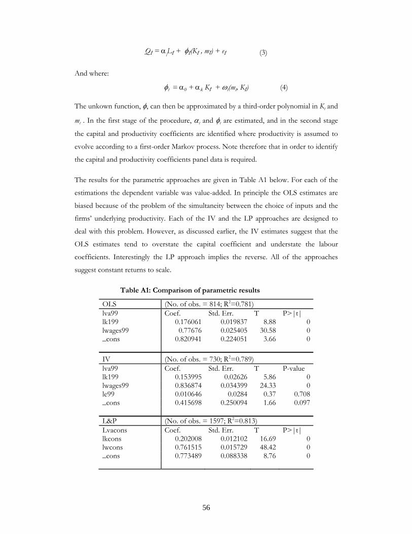
Qt = αlLt + φt(Kt , mt) + et (3)
And where:
φt = α0 + αk Kt + ωt(mt, Kt) (4)
The unkown function, φ, can then be approximated by a third-order polynomial in Kt and
mt . In the first stage of the procedure, αt and φt are estimated, and in the second stage
the capital and productivity coefficients are identified where productivity is assumed to
evolve according to a first-order Markov process. Note therefore that in order to identify
the capital and productivity coefficients panel data is required.
The results for the parametric approaches are given in Table A1 below. For each of the
estimations the dependent variable was value-added. In principle the OLS estimates are
biased because of the problem of the simultaneity between the choice of inputs and the
firms’ underlying productivity. Each of the IV and the LP approaches are designed to
deal with this problem. However, as discussed earlier, the IV estimates suggest that the
OLS estimates tend to overstate the capital coefficient and understate the labour
coefficients. Interestingly the LP approach implies the reverse. All of the approaches
suggest constant returns to scale.
Table A1: Comparison of parametric results
OLS (No. of obs. = 814; R2=0.781) lva99 Coef. Std. Err. T P>|t| lk199 0.176061 0.019837 8.88 0 lwages99 0.77676 0.025405 30.58 0 _cons 0.820941 0.224051 3.66 0 IV (No. of obs. = 730; R2=0.789) lva99 Coef. Std. Err. T P-value lk199 0.153995 0.02626 5.86 0 lwages99 0.836874 0.034399 24.33 0 le99 0.010646 0.0284 0.37 0.708 _cons 0.415698 0.250094 1.66 0.097 L&P (No. of obs. = 1597; R2=0.813) Lvacons Coef. Std. Err. T P>|t| lkcons 0.202008 0.012102 16.69 0 lwcons 0.761515 0.015729 48.42 0 _cons 0.773489 0.088338 8.76 0
57
2.2.2: Non-parametric approach – index numbers: The non-parametric index number approach derives directly from the growth accounting
framework. Assume production can be represented by: Qit= F(Xit, Ait). Where Qit is the
output level of unit i at time t., Xit is a vector of factor inputs of unit i at time t, .and θit
is an index of technology. It can then be shown that:
i.e. the difference in the technology of two units of production (θit & θjt) is a function of
the differences in output differentials, Qit & Qjt, and weighted factor intensities Xkit &
Xkjt , where the weights ski & skj are share of each factor in value added. This index, the
Tornqvist-Theil index is said to be exact & superlative because it can be derived from any
flexible functional form. For comparisons across firms, the comparison is usually made
with respect to a reference firm, eg. to a hypothetical firm with average log output, shares
etc.
The standard index as derived above has the advantages outlined earlier and in particular
that no underlying assumptions are made about the production technology, which can
thus differ across firms. However, a possible disadvantage is that the index assumes
constant returns to scale and perfect competition in both input and output markets.
Klette and Johansen (1999) propose a modification of the above, which at least partially
addresses these issues and involves a two-stage procedure. They derive a performance
index, which takes the following form:
Where we are now using the ^ notation to denote the difference between units. Hence, Ŝt
gives the difference in sales between firms at time t, φ is the share of the variable input
in total revenue, Ltx̂ and Ktx̂ , give the difference in labour and capital inputs across the
firms. Equation 6 is essentially a Tornqvist index where sales have replaced output in the
[ ] [ ][ ] )5(loglog21loglog kijkitkjkijtitjtit XXssQQ −+−−=−θθ
)6(ˆ)ˆˆ(ˆˆ KtKtLtLttt xxxsa −−−= φ
58
Solow residual3. The first stage thus involves calculating the performance index as given
by equation 6. Klette and Johansen then show that:
)7(ˆ1ˆ1ˆ tt
Ktt dxaημ
θμε
−+⎟⎟⎠
⎞⎜⎜⎝
⎛−=
where θ is the productivity parameter of interest, ε is the elasticity of scale, μ is the mark-
up of price over marginal cost, and η is the price elasticity of demand, d is a demand shift
parameter. Hence the performance index depends on the productivity parameter, on the
degree of returns to scale, and on any demand shifts. In the absence of any demand
shifts, under perfect competition, and with constant returns to scale, the performance
index is thus simply equal to the Tornqvist index ( tta θ̂ˆ = ). In the second stage
therefore we estimate,
where the parameter, δ captures either the presence of economies of scale and/or
imperfect competition, and where in the absence of any demand shocks, the error term
on this regression, σt, captures the productivity parameter. Clearly, if δ is significant and
negative than this suggests either deviations from perfect competition, or from constant
returns to scale or both. Note that as in the parametric approach, it could still be the case
that there is a correlation between the capital stock in equation 8, and the error term, in
which case our estimate of δ would be biased upwards. In order to correct for this we
therefore ran two version of equation 8 – in levels and in first differences. The aim of the
latter was to try and remove any systematic correlation between capital and productivity.
The coefficient on δ in the two cases (with t-statistics given in brackets) was –0.34 (-
3.18) when done in first differences, and –0.09 (-3.24) when done in levels. As suggested
above it is likely that the coefficient on the latter is upward biased, and that the former to
some extent controls for this, although clearly there is considerably more measurement
error also in this case. We take these coefficients as representing upper and lower
bounds, and hence the results suggest some evidence of either imperfect competition or
economies of scale.
3 See Klette & Johanson, 1999, p.381.
)8(ˆˆ tKtt xa σδ +=
59
Bibliography
Amiti M, 2004, Trade Liberalisation, intermediate inputs and productivity, working paper.
Baily, M.N., Hulten, C. and D. Campbell (1992). “The distribution of productivity in manufacturing firms”, Brooking Papers: Microeconomics, Washington D.C.
Barnard and Jenson, 2004 , Exporting and Productivity in the USA, Oxford Review of Economic Policy, Vol.20, No.3.
Blundell, R. and S. Bond (1998), “GMM estimation with persistent panel data: an application to production functions”, IFS Working Papers with number W99/04.
Caves, D.W., L.R. Christensen, and E.W. Diewert (1982a). “The Economic Theory of Index Numbers and the Measurement of Input, Output and Productivity”. Econometrica 50 (6), 1393-1414.
Caves, D.W., L.R. Christensen, and E.W. Diewert (1982b). “Multilateral Comparisons of Output, Input, and Productivity using Superlative Index Numbers”. Economic Journal 92, 73-86.
Charnes, A., W.W. Cooper, and E.Rhodes (1978). “Measuring the Efficiency of Decision Making Units”. European Journal of Operational Research 2, 429-444
Christensen, L., D. Jorgensen, and L. Lau (1971). “Conjugate Duality and the Transcendental Logarithmic Production Function”. Econometrica, July, 255-256.
Clerides, S., Lach, S. and J. Tybout, (1998). “Is Learning By Exporting Important? Micro-Dynamic Evidence From Colombia, Mexico, And Morocco,” The Quarterly Journal of Economics, MIT Press, vol. 113(3), pages 903-947
Diewert, W.E. (1976). “Exact and Superlative Index Numbers”. Journal of Econometrics 4, 115-145.
Dollar, David (1992). “Outward-Oriented Developing Countries Really Do Grow More Rapidly: Evidence from 95 LDCs, 1976-85,” Economic Development and Cultural Change, April, 523-544.
Ehui S.K. and Jabbar M.A. (2002). “Measuring productivity in African agriculture: A survey of applications of the superlative index numbers approach”. Socio-economics and Policy Research Working Paper 38. ILRI (International Livestock Research Institute).
Edwards, 1998, Openness, productivity and growth: what do we really know?, Economic Journal, vol.108(2), pp. 383-398.
Fare, R., S. Grosskopf and C.A.K. Lovell (1994), “Production Frontiers”, Cambridge University Press, Great Britain.
Frankel, J. A. and D. Romer (1999). “Does Trade Cause Growth?” The American Economic Review, (June) 379-399.
60
Galal, A. and . Hoekman eds, 1997, Regional Partners in Global Markets: Limits and Possibilities of the Euro-Med Agreements, CEPR/ECES (Egyptian Centre for Economic Studies), London, ch 8
Galal, A. and B. Hoekman eds, 2003, Arab Economic Integration: Between Hope and Reality, ECEC: the Brookings Institutition Press, Washington D.D., 2003, ch 5,
Galal, A. and R.Z. Lawrence eds, 1998, Building Bridges: An Egypt-US Free Trade Agreement, ECES, Cairo and John F. Kennedy School of Government, Cambridge Mass: Brookings Institution Press, Washington DC.
Greenaway, D., Gullstrand, J., Kneller, R., (2004), Exporting may not always firm level productivity, working paper.
Hadi, A. S. (1992), "Identifying Multiple Outliers in Multivariate Data," Journal of the Royal Statistical Society, Series (B), 54, 761-771.
Harrison, A. (1994). “Productivity, imperfect competition and trade reform: Theory and evidence. Journal of International Economics, 36, 53-73.
Klette, J. and F. Johansen, (1996). "Accumulation of R&D Capital and Dynamic Firm Performance: A Not-so-fixed Effect Model," Discussion Papers 184, Research Department of Statistics Norway.
Konan, D. and K. Maskus, 2002, "Quantifying Services Liberalisation in a Small Open Economy, World Bank Working Paper, Washington DC: World Bank.
Levinsohn, J. and A. Petrin (1999), “When Industries Become More Productive, Do Firms?: Investigating Productivity Dynamics” Discussion Paper No. 445, University of Michigan
Liu, L. and J.R. Tybout (1996), “Productivity Growth in Chile and Colombia: The Role of Entry, Exit, and Learning,” in Industrial Evolution in Developing Countries: Micro Patterns of Turnover, Productivity, and Market Structure, edited by Mark J. Roberts and James R. Tybout, Oxford University Press.
Marschak, J. and W. Andrews. (1944). “Random simultaneous equations and the theory of production”. Econometrica, 12(3-4), 143-205.
Maskus, K. and D. Konan, 1997, "Trade Liberalisation in Egypt", Review of Development Economics, 1 (3): 275-93
Oczkowski, E. and Sharma, K. (2001). “Imperfect competition, Returns to Scale and Productivity Growth in Australian Manufacturing: A Smooth Transition Approach to Trade Liberalisation”, International Economic Journal, Vol. 15, Summer 2001.
Olley, S. and A. Pakes (1996). “The dynamics of productivity in the telecommunications equipment industry”. Econometrica, 64 (6), 1263-1298.
Pavcnick, N. (1997). “Trade liberalization, exit, and productivity improvements: Evidence from Chilean plants. Working Paper, Department of Economics, Princeton University.
Roberts, M. J. and J. R. Tybout , eds. (1996), Industrial Evolution in Developing Countries: MicroPatterns of Turnover, Productivity, and Market Structure, Oxford: Oxford University Press.
61
Rodriguez, F. and D. Rodrik (2000). “Trade Policy and Economic Growth: A Skeptic’s Guide to the Cross-National Evidence.” Macroeconomics Annual 2000, Ben Bernanke and Kenneth Rogoff, eds., MIT Press for NBER.
Sachs, J. D. and A. Warner (1995). “Economic Reform and the Process of Global Integration.” Brookings Papers on Economic Activity, (1), 1-118
Tornqvist, L., 1936, “The Bank of Finland's Consumption Price Index”, Bank of Finland Monthly Bulletin 10, 1-8.
Van Biesebroeck, J. (2003), “Revisiting Some Productivity Debates”, NBER Working Paper No 10
Van Biesebroeck, J. (2004). “Robustness of Productivity Estimates”, NBER Working Papers 10303, National Bureau of Economic Research.
Winters, L.A. (2004). “Trade Liberalisation and Economic Performance: An Overview”, Economic Journal, Vol. 114, 4-21.