Determinants of Public Health Outcomes: A Macroeconomic...

Determinants of Public HealthOutcomes: A Macroeconomic

Perspective∗

Francesco Ricci

THEMA

Université de Cergy-Pontoise

33 bd du Port

95011 Cergy-Pontoise, France

[email protected]

and LERNA (Toulouse)

Marios Zachariadis

Department of Economics

University of Cyprus

P.O. Box 20537

1678 Nicosia, Cyprus

[email protected]

February 2006very preliminary and incomplete

Abstract

This paper investigates the nature of the aggregate production func-tion of health services. We build a model to analyze the role of publicpolicy in determining social health outcomes, taking into account house-holds choices concerning education, health related expenditures and sav-ing. In the model, education has a positive external effect on health out-comes. Next, we perform an empirical analysis using a data set covering72 countries from 1961 to 1995. We find strong evidence for a dual roleof education as a determinant of health outcomes. In particular, we findthat society’s tertiary education attainment levels contribute positively tohow many years an individual should expect to live, in addition to the rolethat basic education plays for life expectancy at the individual householdlevel. This finding uncovers a key externality of the educational sectoron the ability of society to take advantage of best practices in the healthservice sector.

Keywords: Education, life expectancy, external effects.

JEL Classification: O30, O40

∗We thank Hippolyte d’Albis and Andreas Savvides for their comments and suggestions.

Determinants of Public Health Outcomes: A Macroeconomic Perspective 1

1 Introduction

In the last few years a branch of literature has developed applying macroeco-

nomic analysis methods to various issues related with social health status. A lot

of attention has been paid to the link between health improvement and economic

growth. Theoretical and empirical work has considered how human capital accu-

mulation, health improvements and technological progress reinforce each other

(e.g. van Zon and Muysken 2001, Blackburn and Cipriani 2002, Chakraborty

2004, Howitt 2005). Some papers have underscored the possibility of multi-

ple development paths, which may explain poverty or low life expectancy traps

(e.g. Galor and Mayer 2002, Chakraborty et al. 2005). Others are concerned

with the possible role played by health in the persistence of income inequality

(e.g. Becker et al. 2003, Deaton 2003). This paper also applies theoretical and

empirical methods from macroeconomics, but to a rather different issue. We ex-

plore the determinants of social health status, paying attention to understand

and quantify the role played by the different factors of an aggregate production

function of health services.

We investigate the nature of the aggregate production function of health ser-

vices. This implicit production function determines average life-expectancy in

the economy. First, this has to account for direct inputs such as goods and ser-

vices provided in the health sector and determinants of hygienic conditions. We

consider two different types of explicit inputs, one rival and another non-rival.

We assume purchases of rival inputs to be mostly driven by overall purchasing

power of consumers as captured by real income per capita. Non-rival inputs

to the health sector are pure public goods, affecting the environment in which

households make their decisions. An example of this is sanitation.

Average health performance also depends on how well health-related knowl-

edge is rooted in society. For instance preventive behavior results from knowl-

edge of risks incurred with hazardous behavior. For the individual this knowl-

edge is determined by his/her education and by access to appropriate informa-

tion. The availability and the diffusion of this information is determined by the

distribution of education across society. Education can therefore play two differ-

ent roles in the aggregate production function of health services. First, the level


of education of the household’s head enhances the longevity of its members. It

seems reasonable in fact that education affects crucial factors such as the under-

standing of treatments or feeding children healthily. Second, the average level

of education in the economy improves its absorption capacity for health-related

technology and ideas.

These two effects play conceptually different roles. The first one operates as a

rival input, benefiting only household members. The second instead determines

the capacity of the heath service sector to take advantage of best practices.

This sector is a high-tech sector and experiences fast technological progress.

Furthermore, efficient use of new medical technologies requires understanding

of scientific findings. The sophisticated character of knowledge transmission and

use in this sector suggests that higher education constitutes its crucial deter-

minant. In contrast, we expect the role of education in enhancing household

members longevity to exhibit strongly diminishing returns. Thus, primary ed-

ucation attainment levels should suffice to capture this latter role of education.

On the other hand controlling for this, any additional effect resulting from the

attainment of tertiary education can then be attributed to the second role of

education discussed above.

In this paper we present a model where rational individuals choose their

educational attainment, their savings, and their consumption of rival health-

related inputs. In this model, educational choices affect future wages but also

have external effects on health outcomes.

We then use data from 72 countries for the period from 1961 to 1995 to test

the empirical validity of the theoretical model. Using initial period averages to

explain end-period life expectancy and utilizing appropriate IV estimates, allows

us to alleviate the inherent endogeneity problem concerning life-expectancy and

education. To further address problems with capturing the direction of causality,

we also consider beginning of period changes in the explanatory variables to

explain end of period changes in life expectancy.

We find that primary and tertiary education have separate positive effects

on life-expectancy. Our main finding, is that tertiary education has at least

as great an impact as primary education on health outcomes across countries.

This suggests the externality role of education in facilitating adoption of best


practices in health is at least as important as the role of basic education that en-

hances health outcomes at the household level. This paper provides evidence of

a form of increasing returns in education, concerning their role in the aggregate

production function of health services. This result is particularly interesting be-

cause previous work has established that primary education is the single most

important determinant of income growth, while higher education is found to

have little explanatory power for this component of welfare (see Sala-i-Martin

et al. 2004). Here, tertiary education is found to be an important determinant

of a second component of welfare, health status.

The next section presents the model and the theoretical results. Data are

described and discussed in section 3. Section 4 describes the empirical analysis

and present the empirical results, while section 5 briefly concludes.

2 A model of education and health investment

Suppose that individuals can live for two periods. All individuals live during the

first period. Each has a probability of surviving to the second period, π ∈ (0, 1).In the households’ perception its members survival probability is an increasing

function of health related rival inputs, m. We consider the isoelastic function

retained by Chakraborty and Das (2005)

π =

⎧⎪⎨⎪⎩ μmε if m <³πμ

´ 1ε

π < 1 if m ≥³πμ

´ 1ε

(1)

Our analysis focuses on the interesting case when m <³πμ

´ 1ε

. We consider that

the following is satisfied

Assumption 1 ε ∈ (0, 1) : Perceived returns on rival inputs to health are

decreasing.

Remark. In the theory that we present the household does not internalize the

effect of education on the survival probability. Although this extension would be

conceptually appealing, it would make the problem untractable as it exacerbates


the issue of endogenous discounting, making the problem non concave in general.

Our simplifying assumption helps emphasize the external effect of education,

whose importance in determining health outcomes is also the main empirical

finding of this paper.

We assume that the effectiveness of health investment, m, in enhancing life

expectancy μ, depends upon the average education level in the economy, e, and

on public health policy according to function h = ζ1Hδ 1−δ, δ ∈ (0, 1), where

H is the level of non-rival health related inputs and is an index of population

density. The level of education in the labor force acts as a pure externality

because it enhances life expectancy by facilitating the use and diffusion of best

practices. Input h is a pure public good, affecting for instance the rate at which

households are subject to diseases. We use a Cobb-Douglas specification

μ ≡ (ζ0e)κ ¡

ζ1Hδ 1−δ¢1−κ

≡ ζeκHδ(1−κ) (2)

where we have defined ζ ≡ ζκ0ζ1−κ1

(1−δ)(1−κ), and assume κ ∈ (0, 1). This isthe basic building block of our theoretical framework which we take to the data.

The household problem consists in choosing education, e, rival health related

inputs, m, and savings, s, to maximize its expected intertemporal utility:

maxc1,c2,s,m,e

u (c1) + πu (c2)

taking into account its sub-period budget constraints:

(1− τ)w [1− (1− τe) e] = c1 + (1− τm) pmm+ s (3)

(1− τ) [w (1 + g (e)) +Rs] = c2 (4)

Education is costly in terms of forgone first period income but increases second

period labor income by g (e) percent, where g0 > 0 and g00 < 0. Savings earn a

gross return R. Public policy affects the household budget in three ways. First,

income is reduced by the income tax, at rate τ . Second, expenditure on rival

health related inputs is subsidized at rate τm. Third, the opportunity cost of


education as expressed in terms of forgone wage income, is reduced by a subsidy

applied at rate τe.1

As Blanchard (1985) and Yaari (1965) we assume that annuity markets exist.

The household considers as given the return on savings, R. Free entry in the

insurance market implies zero profits, i.e. fair insurance premia so that:

R =1 + r

E (π)(5)

where r is the risk-free rate of interest and E (π) denotes the average survival

probability for the generation. In a symmetric equilibrium this price depends

on the individual choice of health related inputs and of education (via 1 and 2).

Our analysis is restricted to the case of a small open economy, where pre-tax

return on savings, r, wages, w, and medical inputs prices, pm, are exogenous

and assumed constant.2 This simplification is useful to focus attention on the

direct interactions between private investment in health and in education, and

on the role of public policy.

2.1 The household’s choice

Let us restate the problem in the following form:

maxs,m,e

u ((1− τ)w [1− (1− τ e) e]− (1− τm) pmm− s)

+ πu ((1− τ) [w (1 + g (e)) +Rs])

the first order conditions for an interior solution are:

u0 (c1) = π (1− τ)Ru0 (c2) (s)

u0 (c1) =π0m

(1− τm) pmu (c2) (m)

u0 (c1) = πg0 (e)

1− τ eu0 (c2) (e)

1Notice that first period gross labor income is w if no education is acquired. Gross incomeis reduced by we0 if an education level e0 is attained. The public subsidy decreases this costby τewe0.

2These restrictions somehow frustrate the macroeconomic approach retained. For instancethe wage could be endogenous on the number of surviving individuals.


Let us pursue the analysis for the case of isoelastic utility functions u (c) =

c1−σ/ (1− σ) and specify g (e) = beβ with β ∈ (0, 1), and by adopting thefollowing3

Assumption 2 σ ∈ (0, 1) : Substitution effects dominate income effects.σ > ε : Perceived returns on health investment are not large enough to convince

households to postpone consumption entirely to the second period.

Then the first order conditions above become:

c−σ1 = π (1− τ)Rc−σ2 (s0)

c−σ1 =ε

m

π

(1− τm) pmc1−σ2 / (1− σ) (m0)

c−σ1 = πβbeβ−1

1− τec−σ2 (e0)

Combining (s0) and (e0) we get:

e = e∗ ≡µ

βb

(1− τ e) (1− τ)R

¶ 11−β

(6)

Notice that education decreases with the net return on savings. This is due

to the fact that education and savings are two competing means to transfer

consumption to the second period.

Combining (m0) and (s0) we get:

c2 = (1− τ)R(1− σ)

ε(1− τm) pmm (7)

where we understand that σ ∈ (0, 1) is a necessary assumption for the problemto make sense. Then from (7) and (4), taking into account (6), we have:

s =1− σ

ε(1− τm) pmm−

w

R

Ã1 + b

µβb

(1− τe) (1− τ)R

¶ β1−β!

(8)

Savings tend to increase with health related expenditure, m, given that σ ∈(0, 1), and to decrease with the level and productivity of education, g (e). Com-

3Chakraborty and Das (2005) retain these same assumptions.


bining (s0) and (7):

c1 =(1− τm) pm

[(1− τ)R]1−σσ

1− σ

επ−

1σm (9)

so that c1 is increasing and concave in m.4

Now we can obtain the solution in terms of the level of health related input,

m. To do this we combine the budget constraint with desired consumption, c1

and c2, and education, e. First substitute for c1 and s in (3) using (9) and (8)

to get:

(1− τ)w [1− (1− τe) e] =(1− τm) pm

[(1− τ)R]1−σσ

1− σ

επ−

1σm

+(1− τm) pmm+ (1− τm) pm1− σ

εm

−wR

Ã1 + b

µβb

(1− τe) (1− τ)R

¶ β1−β!

Define

γ0 ≡ pm

µ1 +

1− σ

ε

¶> pm and γ1 ≡

1− σ

εpm > 0 (10)

and the maximized permanent disposable income, which takes into account the

individually optimal investment in education (6), as5

y ≡ (1− τ)w

∙1− (1− τ e) e

∗ +1 + g (e∗)

(1− τ)R

¸(11)

Using (1), the solution is therefore defined implicitly by :

Γ (m) ≡ γ0 (1− τm)m+γ1μ

− 1σ

[(1− τ)R]1−σσ

(1− τm)m−σ−ε

σ − y = 0 (12)

4Although we have set up a problem with endogenous discounting, the objective functionis concave in m. We know from (1) that π is concave in m, and we have established in (9)that c1 is increasing and concave in m, in (7) that c2 is increasing and linear in m. Thusu (c1) + π (m)u (c2) is increasing and concave with respect to m.

5By definition of e∗ we have that (1− τ)w 1− (1− τe) e∗ +1+g(e∗)(1−τ)R =

(1− τ)w [1− (1− τe) e] +wR

1 + b βb(1−τe)(1−τ)R

β1−β


Assumption 2, σ > ε, is necessary and sufficient for function Γ (m) to be in-

creasing and concave.

2.2 Macroeconomic interaction and the symmetric equi-

librium

Let us now turn to the analysis of stationary symmetric equilibria. Symmetry

implies that the average survival probability for generation t up to date t+1, used

by insurers to compute the fair premium, equals individual survival probability

Et (π) = π (13)

To compute the survival probability we use the average education level in the

older generation labor force, of size Lt−1, (i.e. et−1) to account for the exter-

nality on the efficiency of the health service sector. Suppose that the fertility

rate is n, and all individuals have offsprings, so that births, N , evolve accord-

ing to Nt = (1 + nt−1)Nt−1. The labor force at date t is composed of Lt = Nt

young and Lt−1 =πt−11+nt−1

Nt old (educated) workers. At steady state e, s, prices

and tax instruments are constant. In particular we have et−1 = e = et, and

Lt−1 =π1+nLt .

Recall the definition of survival probability (1) and (2). Considering only

interior solutions (π < π) and taking into account symmetry and stationarity

we get

π = ζeκHδ(1−κ)mε

Then taking into account (6), (5) and (13)

π (m) ≡µ

βb

(1− τ e) (1− τ) (1 + r)

¶ κ1−β−κ ³

ζH(1−κ)δmε´ 1−β1−β−κ

(14)

Combining (6), (14) and (5), (13) we obtain6

e∗ (m) ≡µ

βbζH(1−κ)δmε

(1− τ e) (1− τ) (1 + r)

¶ 11−β−κ

(15)

6Conditions (14) and (15) together imply π = (1− τ) (1 + r) (1− τe) / βb (e∗)β−1 .


This level of education is an increasing function of rival health related inputs,

m, and of their efficiency in improving life expectancy, ζH(1−κ)δ, as well as of

the productivity of education, βb, and of the educational subsidy, τe. Again

we find that education is decreasing in the after-tax return on savings, (1 −τ)(1+r), since education and savings are two competing technologies to transfer

consumption to the second period of life. All these considerations are amplified

by the strength of the externality, κ, due to average education of older workers

on the efficiency of youngsters’ health related investment.

Consider now the first two terms of the implicit function (12), defining the

individually optimal level of health related investment, m. Substituting for the

symmetric equilibrium return on savings, from (5) and (13), then for the survival

probability (14), and taking into account the chosen level of e∗, from (15), we

have

G (m) ≡ γ0 (1− τm)m+γ1

[(1− τ)R]1−σσ

π−1σ (1− τm)m

= (1− τm)m

(γ0 +

γ1

[(1− τ) (1 + r)]1σ

βb (e∗)β−1

1− τe

)(16)

We can also rewrite permanent disposable income, (11), at the symmetric

stationary equilibrium, first substituting for e using (6), next for R using (5)

and (13), then for π using (14), finally exploiting the definition of e∗ (15)

y (m) ≡ (1− τ)w

½1 +

π

(1− τ) (1 + r)+ (1− τe)

1− β

βe∗¾

(17)

It is therefore possible to express the equilibrium decision about private

health investment as being m∗ that solves the following implicit function

Γ (m) ≡ G (m)− y (m) = 0 (18)

Both functions G (m) and y (m) are increasing in m. We are however able to

establish the following proposition under assumption 3.

Assumption 3 ε+β+κ ≤ 1 : Global returns to rival health related inputs aredecreasing.


-

6

m

w

Y

G

m∗

Figure 1: Determining private health investment in a symmetric equilibrium.

κ < (1− β) (1− σ) : Externality of education on the efficiency of health inputs

is not too strong (e.g. κ & 0). Sufficient condition for G0 > 0and G00 < 0.7

Proposition 1 Equation (18) admits a unique, positive and finite, solution if

assumptions 1 to 3 are satisfied.

To prove the result we show in appendix A.1 that G (m) and y (m) are

increasing and concave, that y (0) > G (0) = 0, but y0 declines indefinitely

towards zero while G0 never falls below a positive lower bound. These conditions

imply that the two schedules cross only once, as illustrated in figure 1.

We can use the system (14)-(18) to determine how single policy instruments

affect consumption of rival health related inputs. This is equivalent to assuming

the existence of lump sum taxes to finance public expenditure. We have the

following result

Proposition 2 If changes in policy instruments are financed, or rebated to

households, through lump sum taxes and transfers:

dm

dH> 0 ;

dm

dτm> 0 ;

dm

dτe> 0 ;

dm

dτ< 0

7The sufficient condition for G0 > 0 is actually ε < 1−κ/ (1− β), which is however satisfiedunder this assumption and assumption 2.


For the proof see appendix A.2.

Consider first public health policy as summarized by H and τm. Provision

of non-rival health inputs improves the efficiency of private health inputs and

hence shifts upwards the demand curve for m. Conversely, a subsidy on pur-

chases of private health inputs is tantamount to a downward shift in the supply

curve for m. Both of these measures indirectly imply enhanced educational

attainment (see equation 15). As far as the educational subsidy is concerned,

cheaper education implies more education and this, by itself, makes permanent

disposable income more sensitive to m. As a result it is individually efficient to

consume more m. If moreover education has an external effect improving the

efficiency of m (i.e. if κ > 0), then the response is much stronger as a result

of macroeconomic interaction. We find complementarities between health and

education, giving rise to multiplier effects.

Corollary 3 Combining (14) and proposition 2 we get

dπ

dH>> 0 ;

dπ

dτm> 0 ;

dπ

dτe>> 0

2.3 Public policy

The analysis presented in this subsection does not lead to clear-cut results. This

is not important for the empirical analysis, since we have no comparable cross-

country data on public policy. The reader can skip this subsection.

The other macroeconomic constraint to be considered is the framing of indi-

vidual choices and of public policy. From (18) and (14)-(15) we have established

that individual choices depend on policy instruments τm, H, τ e and τ . While

explaining public policies is beyond the scope of this paper, we still need to

restrict the possibilities set for policy intervention. In particular the scope of

proposition 2 is limited because it assumes the feasibility of public lump-sum

transfers. In practice in many countries education and health account for a sub-

stantial share of public and private expenditure. So any change in the amount

of resources devoted to these sectors is likely to have first order effects on the

rest of the economy, more so as public revenues are usually distortionary.

Since we focus on stationary equilibria, the public budget is assumed to be


held balanced at each period. The public budget constraint equates current

expenditure for generation t, on health and education, to income tax revenue

levied on both generations:

τmpmtmtLt+Ht+τ ewtetLt = τnwt [1− (1− τ e) et]Lt +

hwt

³1 + beβt−1

´+Rtst−1

iLt−1

oUsing the results obtained at the beginning of section 2.2, dividing the budget

by the labor force of young workers and rearranging, public expenditure on

health services per young worker is

τmpmm+H

L= w

∙τ

µ1− (1− τe) e+

¡1 + beβ

¢ π

1 + n

¶− τee

¸+ τRs

π

1 + n

We express the public budget constraint in terms of per-youngster public deficit

and in implicit form, with the help of equations (5), (13), (8) and the definition

of e∗ (15)

PB (m) ≡ H

L+ [τm − τ (1− τm) γ1] pmm− w [τ (1− e∗)− (1− τ) τ ee

∗] = 0

(19)

The first term accounts for expenditure for the provision of non rival health

inputs. The second term accounts for the cost of subsidizing purchases of private

health inputs. Specifically the first term in brackets is public expenditure on

subsidies (τmpmm), while the second term in brackets takes into account the

indirect positive impact on fiscal revenues from taxing savings due to enhanced

life expectancy (i.e. increased m, see equation 8). The third term in (19)

accounts for the income tax revenue from youngsters net of the transfer for

education attainments. In fact the second terms in brackets includes direct

education subsidy payments (τewe∗), but excludes money indirectly recovered

through income taxation (ττewe∗). Hence it is legitimate and plausible to limit

the analysis to the case where policy instruments are constrained to satisfy the

following

Assumption 4 [τm − τ (1− τm) γ1] pm > 0 : Subsidizing purchases of rival

health related inputs is not a self-financing policy.

w [τ (1− e∗)− (1− τ) τee∗] > 0 : Income tax revenue from youngsters is suffi-


cient to finance educational subsidies.

To study the impact of an increase in, say, τm financed through an appro-

priate increase in the income tax rate, τ , one needs to consider how the system

given by equations (18) and (19) adjusts. In this example we have⎧⎨⎩ ∂Γ∂m

dmdτm

+ ∂Γ∂τm

+ ∂Γ∂τ

dτdτm

= 0

∂PB∂m

dmdτm

+ ∂PB∂τm

+ ∂PB∂τ

dτdτm

= 0

implying

dm

dτm=

∂Γ∂τ

³∂PB∂τm

/∂PB∂τ

´− ∂Γ

∂τm

∂Γ∂m −

∂Γ∂τ

¡∂PB∂m /∂PB∂τ

¢Unfortunately, as it is shown in appendix A.3 it is impossible to determine

analytically the sign of this expression. This is not a surprising result to the

extent that the policy takes with one hand what it gives with the other. In

general then the impact is ambiguous.

3 Data description

In this section, we describe the data set we have assembled to test our main

hypotheses and take a first look at the relationship of health status with each

of these inputs. The focus of our study, a country’s health status, is measured

by the average life expectancy at birth.

We employ a number of health output and health input variables from two

sources. TheWorld Development Indicators (WDI) 2002 database provides data

on life expectancy at birth, physicians per thousand people, adult illiteracy

rates8, and sanitation9. We also obtained GDP per capita in PPP dollars,

and tertiary education enrollment rates from the same database. Finally, we

obtained primary and higher education attainment rates from the Barro and

Lee (2001) dataset.

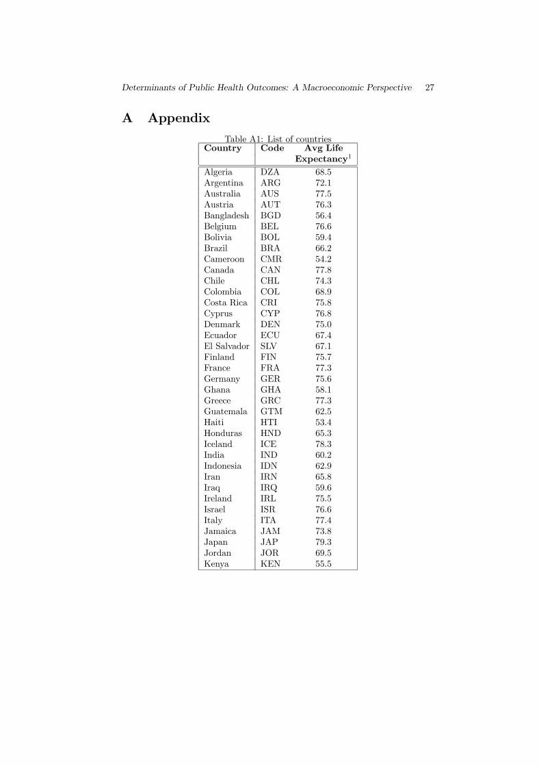
We were able to put together all the above series for 72 countries during the

period 1961-1995. The list of counties is shown in Table A1 in the appendix.8Defined as the percentage of individuals over 15 years of age who cannot, with under-

standing, read and write a short simple statement on their everyday life.9Defined as the percentage of the population with access to improved sanitation facilities.


Table 1: CorrelationsLIFE EDHA EDBA EDH ILLI SAN PHYS INC

LIFE 1EDHA 0.85 1EDBA 0.47 0.33 1EDH 0.88 0.94 0.36 1ILLI -0.73 -0.73 -0.69 -0.74 1SAN 0.77 0.70 0.56 0.69 -0.66 1PHYS 0.89 0.87 0.39 0.91 -0.72 0.73 1INC 0.74 0.77 0.23 0.80 -0.59 0.65 0.86 1Notes: We report cross-sectional correlations after averaging life expectancy over 1990

to 1995 and all remaining (potentially explanatory) variables for the period 1961 to1995, except income for which we use its level at the beginning of the period. Thesample size used here is 72 countries, except for illiteracy rates that is available foronly 53 countries in this sample. All variables are in natural logarithms. LIFE is lifeexpectancy, EDHA is higher education attainment rate, EDBA is primary educationattainment rate, EDH is tertiary education enrollment rate, ILLI is the adult illiteracyrate as a percentage of the population over 15 years of age, SAN is the percentageof the population with access to improved sanitation facilities, PHYS is number ofphysicians per thousand people, INC is initial GDP per capita in constant $US.

However, the great majority of these series are not available annually; in some

cases the data are exceedingly sparse in the time dimension. Because the cross-

sectional dimension of the dataset is more complete and, more importantly,

because of the inherent long-run nature of the relation under study, we chose to

explore empirically the cross-sectional dimension of our dataset.

4 Empirical results

4.1 Preliminary evidence

In Table 1, we report basic correlations between our variables of interest. Our

main hypothesis is that health inputs such us primary and higher education,

sanitation, access to safe water, and physicians availability are related to health

outcomes measured by life expectancy. Indeed, the correlations between life

expectancy and higher education attainment rates or enrollment rates equal 85

and 88 percent respectively, while the correlation for basic education attain-


ment rates equals 47 percent. An other (inverse) measure of basic education

- the adult illiteracy rate - is also strongly correlated with life expectancy at

minus 73 percent. All of these correlations are statistically significant with p-

values below the one percent level. Sanitation and physicians are also strongly

related with life expectancy with correlations of 77 and 89 percent respectively.

However, nearly all of these health inputs are also strongly related to the level

of real income per capita. This is especially true in the case of higher educa-

tion attainment or enrollment rates and for physicians availability. Moreover,

several of these inputs are highly correlated with each other raising a warning

flag regarding a potential collinearity problem in the regression specifications

that follow in the next subsection. Notably, the correlation between higher ed-

ucation attainment or enrollment rates with physicians is 87 and 91 percent

respectively. As a robustness check for the importance of higher education we

will thus consider specifications both with and without the apparently highly

collinear physicians variable.

4.2 Cross-section regression results

We are well aware that there is a strong theoretical argument for endogeneity

between life expectancy and tertiary education. While tertiary education should

be expected to affect health outcomes, it can also be argued that individual de-

cisions on tertiary education attainment depend on expected life expectancy so

that it is plausible that longer life expectancy causes higher tertiary education

levels. However, for the model we consider below, we fail to reject the null

that tertiary education is exogenous with a p-value of 0.31310 and the joint hy-

pothesis that all explanatory variables are exogenous with a p-value of 0.742.

This suggests that we could estimate the empirical model of life expectancy on

secondary and primary education attainment rates, sanitation, physicians, and

initial income with OLS. However, given that we have just about 70 observations

10Treating each explanatory variable as potentially endogenous and the remaining as ex-ogenous, we also fail to reject the null that initial income is exogenous with a p-value of 0.534.Similarly, we cannot reject the null that primary education enrolment is exogenous with ap-value of 0.956. Nor, can we reject the null that physicians is exogenous with a p-value of0.277, and finally we cannot reject the null that sanitation is exogenous with a p-value of0.841.


and that the individual p-values for the null of exogeneity for each explanatory

variable separately range from 0.277 for physicians to 0.956 for primary enroll-

ment rates, we choose to be conservative regarding our inference of exogeneity,

and estimate the model using IV in addition to OLS estimation. This serves to

take into account possible endogeneity problems we have been unable to detect,

and also acts as a robustness check for our OLS results.

Towards the goal of addressing potential endogeneity problems and estab-

lishing some evidence of temporal causation we consider: (i) Using lags of higher

education and the other explanatory variables to explain end-period averages

of life expectancy. Specifically, utilizing the average value of higher education

and the other explanatory variables for 1961-75 to explain the average value

of life expectancy over 1990-95. This takes care of endogeneity if individual

decisions about higher education in 1961-75 are independent of life expectancy

at birth for individuals born between 1990 and 1995. We present results based

on this specification as the "Lags" model in columns two and five in Tables 2

and 3. (ii) Instrumenting the average of tertiary education over 1961-95 by its

average value for 1961-75 to explain the average value of life expectancy over

1990-95. In the regression of each potentially endogenous explanatory variable11

on all exogenous variables, the lag of each explanatory variable is shown to be

strongly significant in determining the explanatory variable’s period average,

with p-values always below the one percent level of significance. We present

results based on the IV specification in columns three and six in Tables 2 and

3.12 (iii) We use log changes in the explanatory variables for the period 1961-75

to explain the log change in life expectancy for the period 1976-95. We also

apply IV estimation to these variables in changes, instrumenting the log change

in tertiary education over 1961-95 by its 1961-75 value. Results based on this

approach are reported in Table 4.

Overall, we assess the link between health inputs and life expectancy with

the "Lags" and "IV" models described above, and the"Period Avg" model where

11Even though we fail to reject the null of exogeneity for any of these variables and jointlyfor all of these variables, we are being conservative in allowing for the possibility that thesecould be endogenous and examine the robustness of the basic OLS results.12We note here that for Sanitation (SAN) we typically have just a handful of observations

for the whole period so we cannot instrument this variable with its lag.


we consider the average of the 1990-95 period life expectancy being explained

by the 1961-95 average value of the explanatory variables. We report results

for this model in columns one and four of Tables 2 and 3. In each case, we

consider specifications with and without physicians, since this variable is highly

collinear with higher education.13 We also consider log changes of the variables

in place of the levels and present estimation results from this exercise in Table

4. In this case, for the "Period Avg" model we consider the growth rate of

life expectancy between 1976 and 1995 being explained by growth rates of the

explanatory variables between 1961 and 1995, with results presented in the first

and fourth columns of Table 4.

The dual effect of education on life expectancy is of primary interest to

us. For this reason, we consider three different specifications with different

pairs of measures for higher and basic education in Tables 2, 3, and 4. In

specification one, we consider higher and primary attainment rates from the

Barro and Lee database. We report the estimates from this specification in

Table 2. In the second specification, results for which are reported in Table 3

we consider tertiary education enrollment rates along with the illiteracy rate,

both taken from the WDI database. Finally, in Table 4, we consider log changes

of education attainment levels.

In Model 1 of Table 2, we consider the impact of basic and higher education

attainment rates as well as real income per capita and sanitation on the end-

period (1990-95) average of life expectancy. We report results from Model 1

in the first three columns of Table 2. Irrespective of whether we consider the

average value of the explanatory variables over the 1961-95 period, their average

value at the beginning of the period, or instrument the former with the latter,

higher education attainment rates consistently have a positive and significant

impact on life expectancy which is always greater than the impact of primary

education. The elasticity of life expectancy with respect to higher education is

13Physicians should have a dual role in determining health outcomes. On the one hand,this is a direct input into the health production function similar to any other medical input.On the other hand, they should have a role as vectors of knowledge facilitating medicaltechnology absorption and the adoption of best practices. Including both tertiary educationand physicians in the same specification should thus be expected to reduce the coefficientestimate of tertiary education to the extent these two variables are capturing the same concept.Thus, the coefficient estimate for tertiary education in these specifications should be seen as alower bound of the importance of the knowledge externality we are focusing on in this paper.


Table 2: Cross-country life expectancy regressionsSpecif. 1 Model 1

Period AvgModel 1

LagsModel 1

IVModel 2Period Avg

Model 2Lags

Model 2IV

INCOME .033∗∗∗(1.75)

.039(1.51)

.039∗∗(2.01)

−.013(−0.82)

−.008(−0.36)

−.004(−0.24)

EDHA .072∗(5.33)

.051∗(3.45)

.063∗(4.24)

.038∗(3.47)

.027∗∗∗(1.69)

.036∗(2.54)

EDBA .048∗∗∗(1.95)

.0411(1.56)

.049∗∗∗(1.70)

.028(1.31)

.019(0.78)

.031(1.21)

SAN .080∗∗∗(1.82)

.101∗∗(2.13)

.087∗∗(2.07)

.066∗∗∗(1.84)

.098∗∗(2.38)

.072∗∗(2.12)

PHYS – – – .070∗(4.29)

.068∗(2.61)

.063∗(3.06)

constant 3.349∗(20.56)

3.307∗(17.76)

3.278∗(18.08)

3.908∗(24.47)

3.834∗(17.74)

3.805∗(20.43)

Adj. R2 78.8 75.3 78.7 82.8 77.9 82.5Obs. 72 72 72 72 71 71Notes: * p-value less than one percent, ** p-value less than five percent, *** p-valueless than ten percent, 1p-value=0.12. For the "Period Avg" models, we consider theaverage of the 1990-95 period life expectancy being explained by the averages of the1961-95 period for the explanatory variables. For the "Lags" models, we consideragain the average of the 1990-95 period life expectancy being explained in this caseby the averages of the 1961-75 period for the explanatory variables. Finally, for the"IV" Models 1 and 2, we instrument the 1961-95 period averages for the explanatoryvariables using their average at the beginning of this period. All variables are in naturallogs so that the reported estimates are elasticities of life expectancy with respect toeach explanatory variable.

stable across the three methodologies ranging between 5.1 percent for the lags

model to 6.3 percent for the instrumental variables estimation, and up to 7.2

percent for the period-averages model. Moreover, the estimated elasticity of life

expectancy with respect to primary education ranges from 4.1 percent with a p-

value of 0.12 for the lags model, to 4.9 and 4.8 percent and statistically significant

at the ten percent level for the IV and period-averages models respectively. For

the three specifications of Model 1, sanitation has a positive and consistently

significant impact on life expectancy estimated about 10 percent.

In Table 2, we also take into account the fact that income can be a ma-

jor determinant of health by including the initial period value of real income

per capita. To the extent to which we control for public health inputs and

education, real income per capita can serve isolate the effect of private health

inputs purchases as it captures the consumer’s purchasing power. Moreover,

controlling for the effect of income helps isolate the effect of each of the other


inputs not related to income. For the specifications in the first three columns,

income has a positive impact on life expectancy, slightly below the elasticity of

life expectancy with respect to primary education.

In columns four to six of Table 2, we report results for Model 2 which now

includes physicians availability in addition to the two education variables, sani-

tation, and income per capita. Since physicians and higher education are highly

collinear, with a correlation of 87 percent, introducing physicians dampens the

impact of higher education on life expectancy. Still, this remains positive and

significant, irrespective of whether we use period-averages, initial period aver-

ages, or instrument the explanatory variables, in columns four, five, and six

respectively. The impact of higher education is stable across the three method-

ologies ranging between 2.7 percent for the lags model to 3.6 percent for the in-

strumental variables estimation and 3.8 percent for the period-averages model.

Once again, the impact of primary education appears positive but is now statis-

tically insignificant while sanitation still has a, somewhat reduced, positive and

significant impact on life expectancy.

Physicians availability has a positive and strongly significant impact on life

expectancy that remains stable at about seven percent in columns four to six,

irrespective of the methodology pursued. To the extent that physicians facilitate

the flow of health-related ideas a component of this health input could poten-

tially be perceived as non-rival, a hypothesis that is supported by the dampening

of the impact of higher education once the physicians availability variable is in-

troduced in Model 2. Finally, once we account for physicians, income now has

no impact on life expectancy.

Next, we consider a different (inverse) measure of basic education - the rate

of illiteracy - along with tertiary education enrollment rates. In Table 3, we

replicate the regression models estimated in Table 2, using now this alternative

measures of basic and higher education. Conceptually, the illiteracy rate should

measure an even more orthogonal component of education than primary attain-

ment rates, relative to what is captured by our measures of tertiary education.

In Table 3, tertiary education enrollment rates are shown to have a positive and

statistically significant impact on life expectancy with elasticities ranging from

a high of 8.5 percent down to 3.5 percent for the different models considered



Period AvgModel 1

LagsModel 1

IVModel 2Period Avg

Model 2Lags

Model 2IV

INCOME .039∗∗(2.08)

.039∗∗∗(1.89)

.038∗∗(2.12)

.006(0.32)

.009(0.37)

.004(0.19)

EDH .085∗(4.98)

.068∗(3.43)

.078∗(4.36)

.055∗(3.27)

.046∗∗(2.21)

.035∗∗∗(1.82)

ILLI −.0281(1.41)

−.002∗∗∗(−1.83)

−.045∗∗(−1.98)

−.021(−1.09)

−.001(−1.22)

−.039∗∗∗(−1.79)

SAN .0332(1.49)

.0333(1.47)

.025(1.16)

.020(0.99)

.0304(1.39)

.011(0.53)

PHYS – – – .054∗(3.34)

.053∗∗(2.03)

.065∗(2.85)

constant 3.65∗(20.96)

3.71∗(21.50)

3.76∗(21.08)

4.03∗(20.64)

4.02∗(17.62)

4.19∗(17.62)

Adj. R2 79.8 76.9 79.8 82.0 78.6 81.9Obs. 61 60 60 61 60 60Notes: * p-value less than one percent, ** p-value less than five percent, *** p-valueless than ten percent, 1p-value=0.16, 2p-value=0.12, 3p-value=0.15, 4p-value=0.17,4p-value=0.115. For the "Period Avg" models, we consider the average of the 1990-95 period life expectancy being explained by the averages of the 1961-95 period forthe explanatory variables. For the "Lags" models, we consider again the average ofthe 1990-95 period life expectancy being explained in this case by the averages of the1961-75 period for the explanatory variables. Finally, for the "IV" Models 1 and 2,we instrument the 1961-95 period averages for the explanatory variables using theiraverage at the beginning of this period. All variables are in natural logs so that thereported estimates are elasticities of life expectancy with respect to each explanatoryvariable.

there. Illiteracy has a negative impact on life expectancy which can be sta-

tistically insignificant once physicians are introduced in the specification. The

impact of sanitation remains positive but is not significant at conventional lev-

els of significance, while the impact of physicians remains positive, significant,

and of similar magnitude as previously. The estimated impact of income is

positive but becomes statistically indistinguishable from zero once we introduce

physicians in Model 2 presented in columns four to six.

Overall, we find that higher education matters significantly, and is more

robust than primary education, sanitation, and even income. Using initial pe-

riod averages to explain end-period life expectancy, allows us to establish that

tertiary education is a significant and robust explanatory variable of end of pe-

riod health output. This approach alleviates potential endogeneity problems

and provides supporting evidence of a causality link from tertiary education to



PeriodAvgModel 1

LagsModel 1

IVModel 2PeriodAvg

Model 2aLags

Model 2bLags

Model 2IV

INCOME −.0002(−0.57)

−.001∗∗(−1.98)

−.0003(−0.65)

−.0003(−0.85)

−.001∗∗(−2.29)

−.001∗∗(−2.04)

−.001(−1.63)

1

EDHA .055∗(3.98)

.025∗(3.17)

.068∗(3.82)

.047∗(3.96)

.025∗(4.42)

.025(2.80)

∗ .069∗(3.56)

EDBA .060∗(2.77)

.032(1.48)

.042(1.18)

.058∗(2.66)

.042∗∗(2.14)

.017(0.85)

.021(0.72)

YGROWTH .030(1.03)

−.015(−0.81)

−.029(−0.85)

.008(0.34)

−.017(−0.86)

−.031(−1.39)

−.061(−1.49)

PHYS .063∗∗(2.34)

.074∗∗(2.48)

.079∗(3.09)

.101∗(2.63)

constant .003(0.81)

.009∗(2.69)

.004(0.94)

.003(0.89)

.007∗∗(2.55)

.009∗∗(2.37)

.006(1.49)

Adj. R2 31.5 22.6 25.5 42.1 41.9 29.7 32.1Obs. 66 66 66 63 63 52 50Notes: * p-value less than one percent, ** p-value less than five percent, *** p-valueless than ten percent, 1p-value=0.104. All variables other than initial real income percapita are in log changes. YGROWTH is the growth rate of real income per capita. Forthe "Period Avg" models, we consider the growth rate of life expectancy between 1976and 1995 being explained by growth rates of the explanatory variables between 1961and 1995. For the "Lags" models, we consider again the growth rate of life expectancybetween 1976 and 1995 being explained by growth rates of the explanatory variablesbetween 1961 and 1975. Finally, for the "IV" Models 1 and 2, we instrument the1961-95 period changes for the explanatory variables using their beginning of periodaverages. In Model 2a we do not use the beginning of the period change for physicianswhich allows us to use about 20% more observations. We do this in Model 2b forcomparability of the sample with the IV Model 2. All variables are in natural logsso that the reported estimates are elasticities of life expectancy with respect to eachexplanatory variable.

health status (life expectancy).

As an additional methodology to remedy potential endogeneity problems

facing tertiary education as a determinant of health status, we consider log

changes of the variables instead of their log levels. This also serves as a robust-

ness check for our main finding regarding the dual importance of education, and

in particular the channel through which higher education affects life expectancy

emphasized in this paper. We report estimates in Table 4.

The growth rate of higher education attainment levels has a positive impact

on the end period growth rate in life expectancy for all seven specifications

we consider below. It takes its highest value of about seven percent in the

IV specifications reported in columns three and seven. The growth rate of


primary education also has a positive effect which is now close to that for tertiary

education but is statistically insignificant in several of the models we consider.

Looking at the negative coefficient estimates for initial income levels, there

appears to be some evidence for convergence in life expectancy for countries that

started with low real income per capita level. On the other hand, the growth

rate of real income per capita does not seem to explain any of the gains in life

expectancy. This suggests that any convergence that took place for initially

low-income countries has not been the result of higher real income per capita

growth, but likely due to changes in other determinants of public health in lag-

gard countries. These other determinants would likely include public inputs like

sanitation (which we cannot consider here directly in the absence of observa-

tions over time for this variable), and perhaps medical knowledge diffusion as

emphasized in Papageorgiou, Savvides, and Zachariadis (2005).

5 Conclusion

We have presented a model where education can have external effects on life

expectancy, beyond what can be expected from the impact of basic education

on the individual household’s health status. Our main results are as follows:

a) Considering physicians per thousand inhabitants as an explanatory variable

we find it extremely significant and robust. As a side effect, introducing this

variable reduces the separate impact of tertiary education. b) Public health

inputs such us sanitation have a positive impact on life expectancy. c) There

is some evidence of convergence in life expectancy for countries that started off

with low real income per capita levels in 1961 and this does not appear to be

explained by faster output growth rates of initially poor countries, suggesting

the possibility that faster technology absorption of initially laggard countries

might actually be behind convergence. d) Education has a dual role in deter-

mining health oucomes, with both basic and higher education having positive

impact on life expectancy. Moreover, the impact of higher education appears

to be at least as important as the impact of basic education in determining life

expectancy, suggesting the externality role of education in facilitating adoption

of best practices in health is at least as important as the role of basic education


enhancing health outcomes at the household level.

The last result is particularly interesting because growth regressions have

established that primary education is the single most important determinant of

income growth, while higher education is found to have little explanatory power

(Sala-i-Martin, Doppelhofer and Miller 2004). Also microeconomic evidence

suggests that primary education is more important than tertiary education in

determining growth in income (e.g. Psacharopoulos 1994). Our findings suggest

that tertiary education might be important for one component of welfare, health

status, even if it’s less important as a determinant of an other component of

welfare, income per capita.


BibliographyAisa, R. and F. Pueyo (2004), “Endogenous longevity, health and economic

growth: a slow growth for a longer life?” Economics Bulletin, Bulletin,9(3), 1-10.

Bhargava, A., Jamison, D., Lauc, L. and C. Murray (2001), “Modeling theeffects of health on economic growth,” Journal of Health Economics, 20,423-440.

Barro, R. (1996), “Health and Economic Growth,” paper presented at the thePan American Health Organization conference on Health, Human Capitaland Economic Growth.

Barro, R. and J-W. Lee (1993), “International Comparisons of EducationalAttainment," Journal of Monetary Economics, 32(3), 363-94.

Becker, G., Philipson, T. and R. Soares (2003), “The Quantity and Qualityof Life and the Evolution of World Income Inequality,” NBER WorkingPaper, No. 9765.

Blackburn, K. and G-P. Cipriani (2002), “A model of longevity, fertility andgrowth,” Journal of Economic Dynamics & Control, 26 187-204.

Blanchard, O. (1985), “Debt , Deficits and Finite Horizons,” Journal of Polit-ical Economy 93, 223-247.

Bloom, D., Canning, D. and J. Sevilla (2004), “The Effect of Health on Eco-nomic Growth: A Production Function Approach,” World Development,32(1), 1?13.

Castelló-Climent, A. and R. Doménech (2004), “Human Capital Inequality,Life Expectancy and Economic Growth,” mimeo, Universidad Carlos IIIde Madrid.

Chakraborty, S. (2004), “Endogenous Lifetime and Economic Growth,” Jour-nal of Economic Theory 116, 119-137.

Chakraborty, S. and M. Das (2005), “Mortality, Human Capital and PersistentInequality,” Journal of Economic growth, forthcoming.

Chakraborty, S., Papageorgiou, C. and F. Pérez-Sebastían (2005) , “Diseaseand Development,” paper presented at the Conference on Health, Demo-graphics and Economic Development, Stanford University.

Commission on Macroeconomics and Health (2001),Macroeconomics and Health:Investing in Health for Economic Development, Geneva: World Health Or-ganization.

Deaton, A; (2003), “Health, Inequality, and Economic Development”, Journalof Economic Literature 41, 113-158.


Devlin, N. and P. Hansen (2001), “Health care spending and economic output:Granger causality,” Applied Economics Letters, 8(8), 561-563.

Ehrlich, I. and H. Chuma (1990), “A Model of The Demand for Longevity andthe Value of Life Extension,” Journal of Political Economy 98, 761-782.

Fogel, R. (1994), “Economic Growth, Population Theory, and Physiology:The Bearing of Long-Term Processes on the Making of Economic Policy,”American Economic Review 84, 369-95.

Fogel, R. (1997), “New Findings on Secular Trends in Nutrition and Mortal-ity: Some Implications for Population Theory,” in M. Rosenzweig and O.Stark (eds.), Handbook of Population and Family Economics. Amster-dam: Elsevier, 433-81.

Frankel, J.A. and D. Romer (1999), “Does Trade Cause Growth,” AmericanEconomic Review 89, 379-99.

Galor, O. and D. Mayer-Foulker (2002), “Food for Thought: Basic Needs andPersistent Educational Inequality,” paper presented at the the Pan Amer-ican Health Organization conference on Health, Human Capital and Eco-nomic Growth, forthcoming in G. Lopez-Casasnovas, B. Rivera and L.Currais (eds.), Health and Economic Growth: Findings and Policy Impli-cations. Cambridge, MA: MIT Press.

Grossman, M. (1972), “On the Concept of Health Capital and the Demand forHeath,” Journal of Political Economy 80, 223-250.

Gupta, S., Verhoeven, M. and E. Tiongson (2001), “Public Spending on HealthCare and the Poor,” IMF working paper 01/127.

Hall, R. and C. Jones (1999), “Why Do Some Countries Produce so MuchMore Output Per Worker than Others?,” Quarterly Journal of Economics114, 83-116.

Hall, R. and C. Jones (2004), “The Value of Life and the Rise in Health Spend-ing,” NBER Working Paper Series, No. 10737.

Jamison, D., Lau, L. and J. Wang (2005), “Health’s Contribution to EconomicGrowth in an Environment of Partially Endogenous Technical Progress,”forthcoming in G. Lopez-Casasnovas, B. Rivera and L. Currais (eds.),Health and Economic Growth: Findings and Policy Implications. Cam-bridge, MA: MIT Press.

Kalemli-Ozcan, S. (2002) “Does the Mortality Decline Promote EconomicGrowth?”, Journal of Economic Growth, 7, 411-439.

Neumayer, E. (2003), “Beyond income: convergence in living standards, bigtime,” Structural Change and Economic Dynamics, 14, 275-296.


Nordhaus, W. (2002), “The Health of Nations: The Contribution of ImprovedHealth to Living Standards,” NBER working paper 8818.

Pritchett, L. and L. Summers (1996), “Wealthier is Healthier,” Journal ofHuman Resources, 31(4), 841-868.

Papageorgiou, C., Savvides, A. and M. Zachariadis (2005), “International Med-ical R&D Spillovers,” mimeo University of Cyprus.

Psacharopoulos, G. (1994) “Returns to investment in education: a global up-date,” World Development, 22(9), 1325—1343.

Romer, P. (1990), “Endogenous Technological Change,” Journal of PoliticalEconomy 98, S71-S96.

Sala-i-Martin, X., Doppelhofer, G. and R. Miller (2004), “Determinant of Long-term Growth: A Bayesian Averaging of Classical Estimates (BACE) Ap-proach,” American Economic Review 94(4), 813-835.

Stern M. (2003), “Endogenous Time Preference, Fertility, and Optimal Growth,”Working Paper, Indiana University.

Thomas, D. and E. Frankenberg (2002), “Health, nutrition and prosperity: amicroeconomic perspective,” Bulletin of the World Health Organization,80, 106-113.

Usher, D. (1973), “An Imputation to the Measure of Economic Growth forChanges in Life Expectancy,” in M. Moss, ed., The Measurement of Eco-nomic and Social Performance, New York: NBER.

van Zon, A. and J. Muysken (2001), “Health and endogenous growth,” Journalof Health Economics, 20, 169?185.

Weil, D. (2005), “Accounting for the Effect of Health on Economic Growth,”paper presented at the Conference on Health, Demographics and EconomicDevelopment, Stanford University.

Yaari, M. (1965), “Uncertain lifetime, life insurance, and the theory of theconsumer,” Review of Economic Studies 32, 136-150.

Younger, S. (2001), “Cross-Country Determinants of Declines in Infant Mor-tality: A Growth Regression Approach,” mimeo Cornell University.


A AppendixTable A1: List of countries

Country Code Avg LifeExpectancy1

Algeria DZA 68.5Argentina ARG 72.1Australia AUS 77.5Austria AUT 76.3Bangladesh BGD 56.4Belgium BEL 76.6Bolivia BOL 59.4Brazil BRA 66.2Cameroon CMR 54.2Canada CAN 77.8Chile CHL 74.3Colombia COL 68.9Costa Rica CRI 75.8Cyprus CYP 76.8Denmark DEN 75.0Ecuador ECU 67.4El Salvador SLV 67.1Finland FIN 75.7France FRA 77.3Germany GER 75.6Ghana GHA 58.1Greece GRC 77.3Guatemala GTM 62.5Haiti HTI 53.4Honduras HND 65.3Iceland ICE 78.3India IND 60.2Indonesia IDN 62.9Iran IRN 65.8Iraq IRQ 59.6Ireland IRL 75.5Israel ISR 76.6Italy ITA 77.4Jamaica JAM 73.8Japan JAP 79.3Jordan JOR 69.5Kenya KEN 55.5


Table A1: List of countries cont.

Country Code Avg LifeExpectancy

Korea KOR 71.0Malawi MWI 43.4Malaysia MYS 71.2Mali MLI 44.3Mauritius MUS 70.1Mexico MEX 71.4Mozambique MOZ 43.8Myanmar MMR 55.3Netherlands NET 77.1New Zealand NZL 75.9Norway NOR 77.2Pakistan PAK 59.9Panama PAN 73.0Paraguay PRY 68.6Peru PER 66.8Philippines PHI 66.6Portugal PRT 74.1Sierra Leone SLE 35.2Singapore SGP 75.5Spain ESP 76.8Sri Lanka LKA 70.8Sudan SDN 53.1Sweden SWE 78.1Switzerlannd SWI 77.9Tanzania TZA 49.3Thailand THA 69.1Tunisia TUN 70.8Turkey TUR 67.2Uganda UGA 45.4United Kingdom GBR 76.2Unites States USA 75.5Uruguay URY 73.0Venezuela VEN 71.8Zambia ZMB 47.8Zimbabwe ZWE 53.6

1This is the end of period average life expectancy from 1990 to 1995.

Date post:	16-Mar-2018
Category:	Documents
Upload:	ngoduong
View:	214 times
Download:	1 times

Determinants of Public Health Outcomes: A Macroeconomic...

Documents