Page 1
North Carolina Agricultural and Technical State University North Carolina Agricultural and Technical State University
Aggie Digital Collections and Scholarship Aggie Digital Collections and Scholarship
Theses Electronic Theses and Dissertations
2013
Determination Of Adhesive Strength And Freezing Rate Of Ice On Determination Of Adhesive Strength And Freezing Rate Of Ice On
Aircraft Structures At Subcooled Temperatures Aircraft Structures At Subcooled Temperatures
Elijah Mendoza Kibler North Carolina Agricultural and Technical State University
Follow this and additional works at: https://digital.library.ncat.edu/theses
Recommended Citation Recommended Citation Kibler, Elijah Mendoza, "Determination Of Adhesive Strength And Freezing Rate Of Ice On Aircraft Structures At Subcooled Temperatures" (2013). Theses. 297. https://digital.library.ncat.edu/theses/297
This Thesis is brought to you for free and open access by the Electronic Theses and Dissertations at Aggie Digital Collections and Scholarship. It has been accepted for inclusion in Theses by an authorized administrator of Aggie Digital Collections and Scholarship. For more information, please contact [email protected] .
Page 2
Determination of Adhesive Strength and Freezing Rate of Ice on Aircraft Structures at
Subcooled Temperatures
Elijah Mendoza Kibler
North Carolina A&T State University
A thesis submitted to the graduate faculty
in partial fulfillment of the requirements for the degree of
MASTER OF SCIENCE
Department: Mechanical Engineering
Major: Mechanical Engineering
Major Professor: Dr. John P. Kizito
Greensboro, North Carolina
2013
Page 3
i
School of Graduate Studies
North Carolina Agricultural and Technical State University
This is to certify that the Master’s Thesis of
Elijah Mendoza Kibler
has met the thesis requirements of
North Carolina Agricultural and Technical State University
Greensboro, North Carolina
2013
Approved by:
Dr. John P. Kizito
Major Professor
Dr. Cynthia K. Waters
Committee Member
Dr. Vinayak N. Kabadi
Committee Member
Dr. Sanjiv Sarin
Dean, The Graduate School
Dr. Samuel Owusu-Ofori
Department Chair
Page 4
ii
© Copyright by
ELIJAH MENDOZA KIBLER
2013
Page 5
iii
Biographical Sketch
Elijah Mendoza Kibler was born on July 9, 1988 in Washington, D.C. He attended North
Carolina Agricultural and Technical State University, where he graduated with his Bachelors of
Science in mechanical engineering with highest honors in 2011. From 2010 to 2013, he
conducted research for the NASA Center of Aviation Safety at North Carolina Agricultural and
Technical State University. In 2012 he received support for his research from the National Space
Grant College Fellowship Program, and the North Carolina Space Grant Consortium, receiving
the North Carolina Space Grant for 2012-13. Elijah Mendoza Kibler is a candidate for the
Master of Science in Mechanical Engineering at North Carolina Agricultural and Technical State
University in Greensboro, North Carolina.
Page 6
iv
Dedication
This thesis is dedicated to all of my family and friends, and my nephew Byron L.
Jefferson II. Thank you all for your support; love you all.
Page 7
v
Acknowledgments
First and foremost I thank God for all of the blessings that he has bestowed upon me;
with Him, all things are possible. I would like to thank my friends and family who have stood by
and supported me throughout life and my educational career. I would like to express my
appreciation and gratitude to Dr. John P. Kizito; thank you advising me throughout my years as a
graduate. I would also like to thank all of the graduate researchers that are part of Dr. John P.
Kizito’s Astronautics and Thermofluids Lab for their assistance and support throughout my
graduate experience. Lastly, I would like to thank the NASA University Research Center
(funding grant #NNX09AV08A), NASA Center of Aviation Safety, the National Space Grant
College Fellowship Program, and the North Carolina Space Grant Consortium.
Page 8
vi
Table of Contents
CHAPTER 1 Introduction .................................................................................................................... 3
CHAPTER 2 Literature Review .......................................................................................................... 5
2.1. History of Aircraft Icing ................................................................................................... 5
2.2. Ice Formation on Aircraft Propulsion Systems and Lifting Surfaces ............................ 7
2.2.1. Heterogeneous and homogeneous nucleation processes. ............................... 8
2.2.2. Performance degradation on lifting surfaces due to icing. ........................... 15
2.2.3. Performance degradation on propulsion systems due to icing. .................... 19
2.3. Anti-Icing and De-Icing Techniques ............................................................................. 20
2.3.1. Chemical surfactants. ...................................................................................... 21
2.3.2. Mechanical systems. ....................................................................................... 25
2.3.3. Thermal heating. .............................................................................................. 27
2.4. Shear Strength of Ice on Aircraft Structures ................................................................. 28
2.5. Shadowgraphing Visualization Technique .................................................................... 31
2.6. Definition of Wettability ................................................................................................ 32
2.6.1. Hydrophobic and superhydrophobic surfaces. .............................................. 35
2.6.2. Hydrophilic and superhydrophilic surfaces. .................................................. 35
2.6.3. Ice-phobic surfaces.......................................................................................... 36
2.7. Literature Review Conclusion........................................................................................ 37
Page 9
vii
CHAPTER 3 Methods and Materials ................................................................................................ 38
3.1. Determination of the Adhesive Strength of Ice on Various Substrates ....................... 38
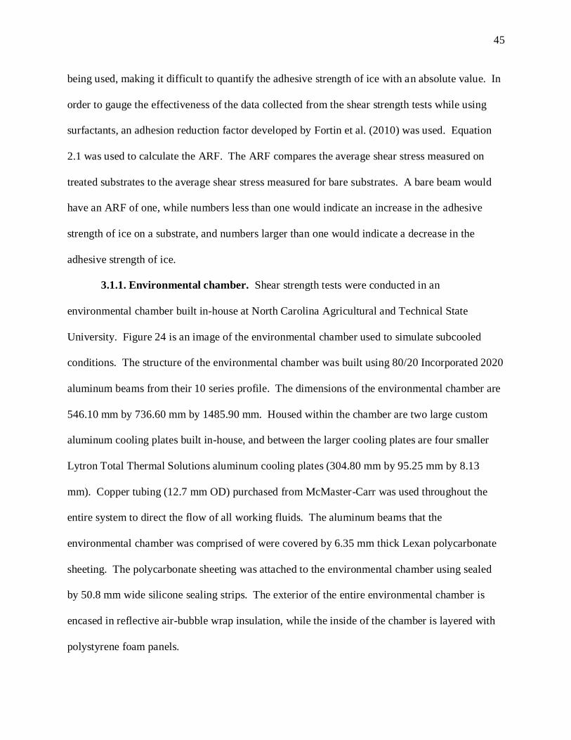
3.1.1. Environmental chamber. ................................................................................. 45
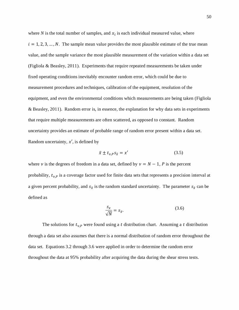
3.1.2. Uncertainty analysis. ....................................................................................... 49
3.2. Determination of Contact Angles .................................................................................. 51
3.3. Visualization and Measurement of Freezing Rate of Sessile Droplets ....................... 56
3.4. Heat Transfer Lumped System Analysis ...................................................................... 64
CHAPTER 4 Results .......................................................................................................................... 72
4.1. Adhesive Strength of Ice on Various Substrates at Subcooled Temperatures ............ 72
4.2. Measurement of Wettability on Surfactant Treated Substrates.................................... 97
4.3. Observation of Freezing Sessile Droplets in a Subcooled Environment ................... 105
4.3. Heat Transfer Lumped System Analysis of a Supercooled Droplet .......................... 110
CHAPTER 5 Discussion and Future Research ............................................................................... 112
References ......................................................................................................................................... 115
Appendix. Collection of raw data from adhesive shear strength tests ........................................... 123
Page 10
viii
List of Figures
Figure 1. Weather related accidents that were reported by the Aircraft Owners and Pilots
Association between 1990 and 2000 .................................................................................. 6
Figure 2. Schematic of the free energy with respect to the radius of the developing nucleus ........ 9
Figure 3. Schematic of change in free energy with respect to radius and temperature ................. 11
Figure 4. Schematic of the free energy versus the radius of a nucleus with respect to the acting
nucleation process ............................................................................................................. 12
Figure 5. (a) Phosphorescence images and (b) Lifetime-based MTT results of the phase
changing process within a freezing water droplet ........................................................... 14
Figure 6. The average temperature of the remaining liquid in the freezing droplet with respect to
time ..................................................................................................................................... 15
Figure 7. Comparison of airflow around (a) a clean airfoil and (b) an airfoil with ice adhered to
its leading edge .................................................................................................................. 16
Figure 8. Lift coefficient of a clean airfoil and an airfoil with ice adhered to its leading edge with
respect to angle of attack ................................................................................................... 17
Figure 9. Schematic of the initial stages of flight ............................................................................ 19
Figure 10. Schematic of the how the micelle polymer interacts to changes in temperature ......... 22
Figure 11. Images of a liquid droplet interacting with an aluminum plate treated with the micelle
polymer ............................................................................................................................. 23
Figure 12. Results of ice removal tests using (a) an elastic ceramic coating and (b) an ice-phobic
Du Pont coating ................................................................................................................ 24
Figure 13. Results from a test comparing failure time of a glycol based freezing depressant to
the average precipitation rate of ice ................................................................................ 25
Page 11
ix
Figure 14. Schematic of a pneumatic boot used on commercial aircrafts ..................................... 26
Figure 15. Schematic of an experimental setup used by to determine the shear strength of the
bond between ice and a substrate .................................................................................... 29
Figure 16. Schematic of the experimental setup for the shadowgraphing technique .................... 31
Figure 17. Images of a heated water jet (a) before and (b) after the jet was activated using the
shadowgraphing technique .............................................................................................. 32
Figure 18. Schematic of a liquid droplet at equilibrium on a flat ................................................... 33
Figure 19. Potassium chloride induced sessile droplet on a substrate subject to voltage ............. 34
Figure 20. Configuration of the fishing wire used in the present study ......................................... 40
Figure 21. Schematic of a substrate frozen within ice in a section of the modified ice tray ........ 41
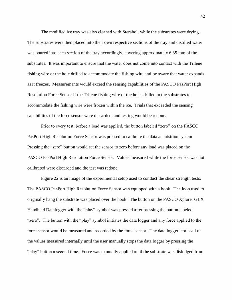
Figure 22. Experimental setup for the shear strength tests ............................................................. 43
Figure 23. Ice cracked due to the application of cyclic loading ..................................................... 44
Figure 24. Environmental chamber used to simulate subcooled conditions .................................. 46
Figure 25. Environmental chamber (a) before and (b) after installing polystyrene panels........... 47
Figure 26. Schematic of the experimental setup used to observe the contact angles of droplets on
the substrates used throughout the present study ........................................................... 52
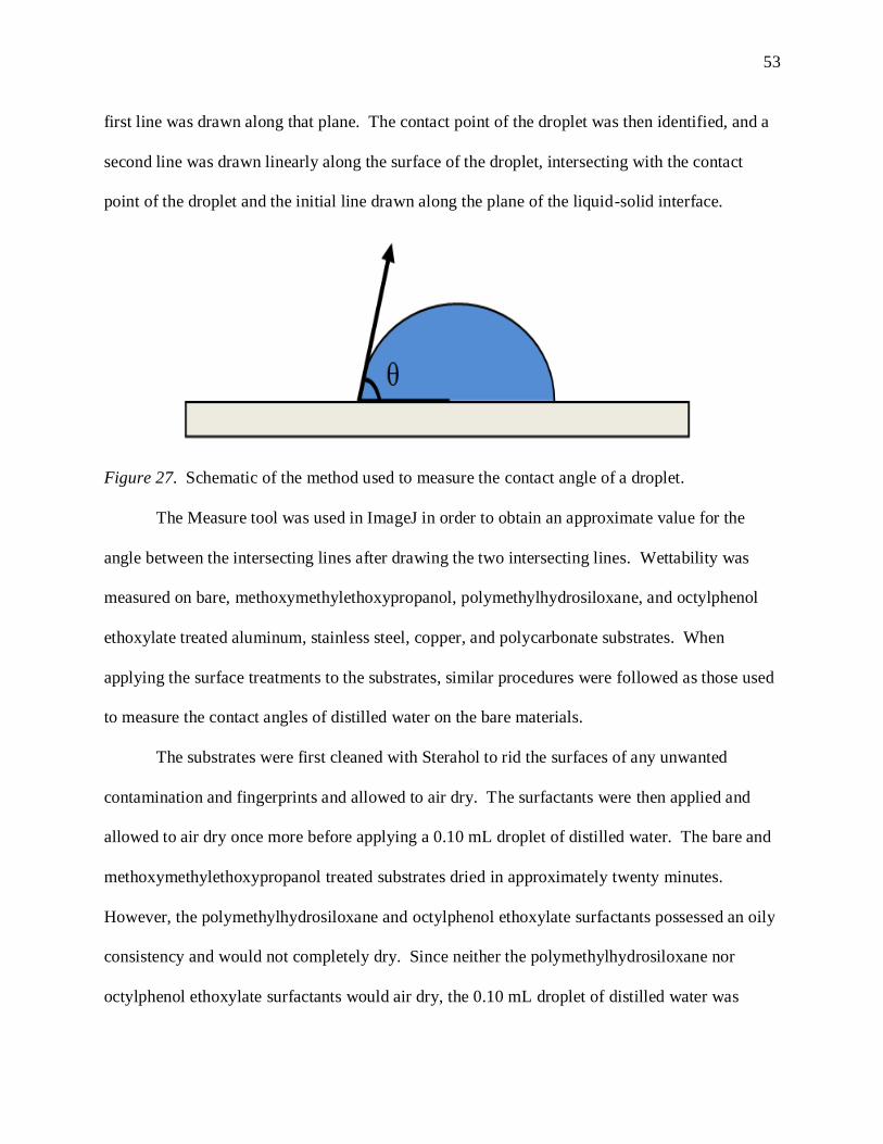
Figure 27. Schematic of the method used to measure the contact angle of a droplet ................... 53
Figure 28. Schematic of the experimental setup used to observe the freezing of a sessile droplet
........................................................................................................................................... 57
Figure 29. Experimental setup used to visualize freezing sessile droplets .................................... 58
Figure 30. Schematic of the experiment setup used to visualize freezing in silicone oil.............. 64
Figure 31. Schematic of the condition simulated using heat transfer lumped system analysis .... 65
Page 12
x
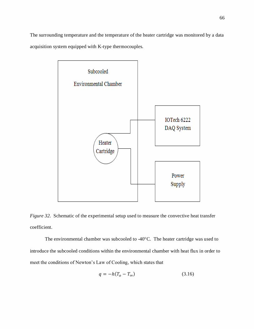
Figure 32. Schematic of the experimental setup used to measure the convective heat transfer
coefficient ......................................................................................................................... 66
Figure 33. Adhesive strength of ice on bare aluminum at -5, -10, -20, and -30C ....................... 73
Figure 34. Average adhesive strength of ice on bare substrates ..................................................... 75
Figure 35. Average adhesive strength of ice on methoxymethylethoxypropanol treated substrates
........................................................................................................................................... 77
Figure 36. Average adhesive strength of ice on polymethylhydrosiloxane treated substrates ..... 80
Figure 37. Average adhesive strength of ice on octylphenol ethoxylate treated substrates .......... 83
Figure 38. Average adhesive strength of ice on the variations of aluminum substrates ............... 85
Figure 39. Average adhesive strength of ice on the variations of stainless steel substrates ......... 88
Figure 40. Adhesive strength of ice on the variations of copper substrates................................... 91
Figure 41. Adhesive strength of ice on the variations of polycarbonate substrates ...................... 94
Figure 42. Summary of all of the average adhesive strength data collected in the present study.
........................................................................................................................................... 97
Figure 43. Sessile droplet on bare (a) aluminum, (b) stainless steel, (c) copper, and (d)
polycarbonate substrates .................................................................................................. 98
Figure 44. Sessile droplet on methoxymethylethoxypropanol treated (a) aluminum, (b) stainless
steel, (c) copper, and (d) polycarbonate substrates ...................................................... 100
Figure 45. Sessile droplet on polymethylhydrosiloxane treated (a) aluminum, (b) stainless steel,
(c) copper, and (d) polycarbonate substrates ................................................................ 102
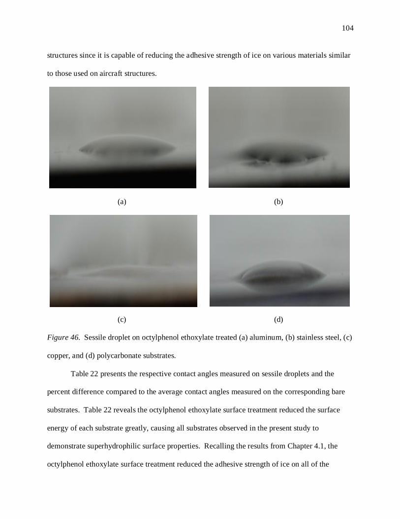
Figure 46. Sessile droplet on octylphenol ethoxylate treated (a) aluminum, (b) stainless steel, (c)
copper, and (d) polycarbonate substrates ..................................................................... 104
Figure 47. Schematic of the freezing process of a sessile droplet ................................................ 106
Page 13
xi
Figure 48. Images of a sessile droplet freezing at subcooled temperatures recorded using high
speed imaging ................................................................................................................. 106
Figure 49. Freezing observed in polystyrene test section on (a) aluminum test stand and (b)
polycarbonate window ................................................................................................... 108
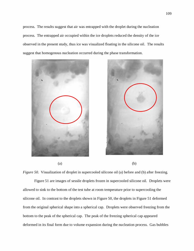
Figure 50. Visualization of droplet in supercooled silicone oil (a) before and (b) after freezing.
......................................................................................................................................... 109
Figure 51. Sessile droplets (a) before and (b) after freezing in supercooled silicone oil ............ 110
Figure 52. Lumped system analysis performed on a spherical droplet in a subcooled
environment .................................................................................................................... 111
Page 14
xii
List of Tables
Table 1. Results of ice adhesion tests conducted throughout literature. ........................................ 30
Table 2. Results of a temporal independent study performed on the code written for heat transfer
lumped system analysis ...................................................................................................... 71
Table 3. Summary of the adhesive strength of ice on bare aluminum at -5, -10, -20, and -30C.
.............................................................................................................................................. 74
Table 4. Summary of the adhesive strength of ice on bare substrates............................................ 76
Table 5. Summary of the adhesive strength of ice on methoxymethylethoxypropanol treated
substrates. ............................................................................................................................ 78
Table 6. ARF and percent difference of methoxymethylethoxypropanol treated substrates. ....... 79
Table 7. Summary of the adhesive strength of ice on polymethylhydrosiloxane substrates. ....... 81
Table 8. ARF and percent difference of polymethylhydrosiloxane treated substrates. ................ 82
Table 9. Summary of the adhesive strength of ice on octylphenol ethoxylate treated substrates.83
Table 10. ARF and percent difference of the octylphenol ethoxylate treated substrates. ............. 84
Table 11. Summary of the average adhesive strength of ice on all variations of aluminum
substrates. ........................................................................................................................... 86
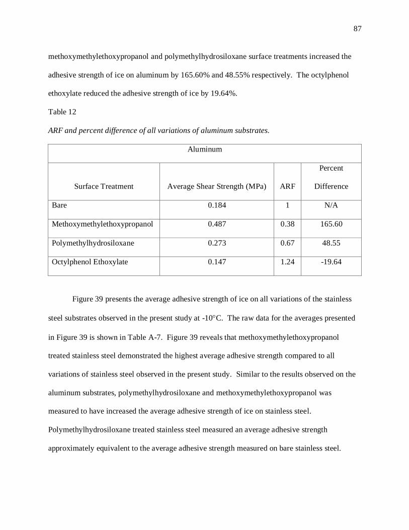
Table 12. ARF and percent difference of all variations of aluminum substrates. ......................... 87
Table 13. Summary of the average adhesive strength of ice on all variations of stainless steel
substrates. ........................................................................................................................... 89
Table 14. ARF and percent difference of all variations of stainless steel substrates. ................... 90
Table 15. Summary of the average adhesive strength of ice on all variations of copper substrates.
............................................................................................................................................ 92
Table 16. ARF and percent difference of all variations of copper substrates. ............................... 93
Page 15
xiii
Table 17. Summary of the average adhesive strength of ice on all variations of polycarbonate
substrates. ........................................................................................................................... 95
Table 18. ARF and percent difference of all variations of polycarbonate substrates.................... 96
Table 19. Contact angles measurements of sessile droplets on bare substrates. ........................... 99
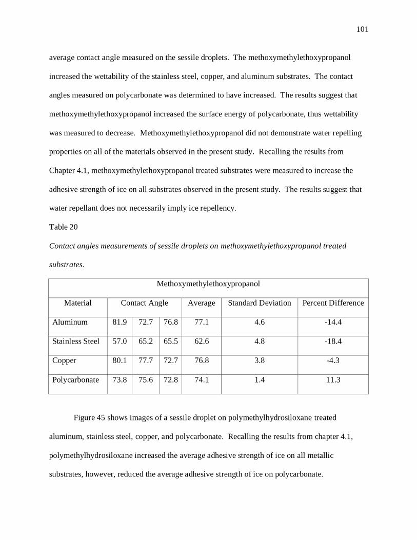
Table 20. Contact angles measurements of sessile droplets on methoxymethylethoxypropanol
treated substrates. ............................................................................................................ 101
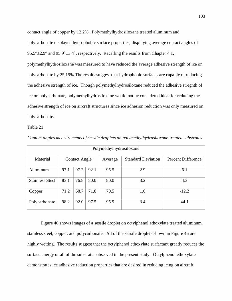
Table 21. Contact angles measurements of sessile droplets on polymethylhydrosiloxane treated
substrates. ......................................................................................................................... 103
Table 22. Contact angles measurements of sessile droplets on octylphenol ethoxylate treated
substrates. ......................................................................................................................... 105
Table A-1. Adhesive strength of ice on bare aluminum at -5, -10, -20, and -30C .................... 123
Table A-2. Adhesive strength of ice on bare substrates ................................................................ 125
Table A-3. Adhesive strength of ice on methoxymethylethoxypropanol treated substrates. ..... 125
Table A-4. Adhesive strength of ice on polymethylhydrosiloxane treated substrates. ............... 126
Table A-5. Adhesive strength of ice on octylphenol ethoxylate treated substrates. .................... 127
Table A-6. Adhesive strength of ice on the variations of aluminum substrates. ......................... 127
Table A-7. Adhesive strength of ice on the variations of stainless steel substrates. ................... 128
Table A-8. Adhesive strength of ice on the variations of copper substrates................................ 129
Table A-9. Adhesive strength of ice on the variations of polycarbonate substrates. .................. 129
Page 16
2
Abstract
Icing is widely recognized as one of the most dangerous, and potentially fatal, weather hazards in
aircraft operations. Ice accretion on lifting surfaces is known to increase flow separation and
drag, decrease lift, alter the moment and pitch of an aircraft, and cause undesired vibrations
throughout the aircraft structure, all of which can lead to loss of control of an aircraft and
accidents. It is for these reasons that developing methods to deter ice adhesion to aircraft
structures is important to the aircraft operations. The average adhesive strength of ice on
aluminum at -5, -10, -20, and -30C, was measured to be 0.2150.031, 0.1840.031,
0.2130.041, and 0.2020.035 MPa respectively, suggesting that temperature does not affect on
the adhesive strength of ice. The adhesive strength of ice was then measured on bare and
methoxymethylethoxypropanol, polymethylhydrosiloxane, and octylphenol ethoxylate treated
aluminum, stainless steel, copper, and polycarbonate substrates at -10C. None of the surfactants
used in the present study were found to be truly ice-phobic. Wettability was measured on the
surfaces of all substrates used. The octylphenol ethoxylate, a surfactant that caused all of the
materials observed in the present study to exhibit superhydrophilic surface properties, was
revealed to be the only surfactant to reduce the adhesive strength of ice on all of the substrates.
At -40C the volumetric freeze rate of a sessile droplet was measured to be 4.62 mm3/second,
and the duration of the entire freezing process of a sessile droplet was 10.67 seconds.
Page 17
3
CHAPTER 1
Introduction
Icing is widely recognized as one of the most dangerous, and potentially fatal, weather
hazards in aircraft operations. Icing can occur while an aircraft is in-flight or on the ground,
causing increases in drag, decreases in lift, changes in the aircrafts pitch and moment, turbulence,
and undesired flow separation, all of which can ultimately lead to loss of control of an aircraft.
Aircraft icing not only affects the aerodynamics of the aircraft, but also poses a threat to aircraft
engines as well, having the potential to accrete on propeller and compressor blades, extinguish
the flames in combustion chambers, and cause complete power loss. Throughout years of
research in aircraft icing, anti-icing and de-icing techniques have been developed, each with its
own benefits and drawbacks. No single anti-icing or de-icing technique has been proven to
completely deter ice accretion without any disadvantages.
The primary goals of aircraft ice protection are to avoid, detect, and recover from any
degradation of an aircraft caused by icing conditions and environments (Reehorst et al., 2010).
The motivation of the present study is based on the need derived from the National Aeronautics
and Space Administration (NASA), in an effort to contribute to aircraft ice protection and safety.
The specific objectives of the present study are to determine:
The adhesive strength of ice on various substrates at subcooled temperatures,
The wettability of surfactant treated substrates,
The freezing rate of sessile droplets using shadowgraphing techniques.
Chapter two entails a literature review of previous studies that have been conducted in the
area of aircraft icing. Chapter two begins with a slight history on aircraft icing, followed by a
more detailed section on the degradation of an aircraft caused by ice, and anti-icing and de-icing
Page 18
4
techniques currently being researched. Chapter three describes the experimental setup and
procedures done to fulfill the specific objectives of the present study. Chapter four describes the
results of all of the experiments done as they pertain to the specific objectives. Finally, Chapter
five concludes the present study based on the results presented in Chapter four, and suggests
areas to be considered for further studies.
Page 19
5
CHAPTER 2
Literature Review
2.1. History of Aircraft Icing
Aircraft icing has been a hazard that has plagued aircraft safety for decades. NASA has
been conducting research efforts towards the detection and prevention of the occurrence and
accumulation of icing on aircrafts, as well as the removal of ice from aircraft structures, since
1928 (Atchison & Bohn, 1981; Geer & Scott, 1930). In the 1950s, NASA’s persistent research
in aircraft icing helped lead to solutions in in-flight aircraft icing for large transport aircrafts, and
in 1981 NASA initiated a new focus in their research: icing protection for small aircrafts and
helicopters (Atchison & Bohn, 1981). The research in icing protection for small aircrafts and
helicopters was due in-part to increases in the purchase of private planes, certification of private
pilots, and the lack of de-icing and anti-icing capabilities available to helicopters. The increase
in private pilots becoming certified came with an increase in pilots lacking the knowledge,
experience, and skill necessary to operate an aircraft under icing conditions (Geer & Scott, 1930;
Reehorst et al., 2010).
Figure 1 shows statistics of weather related accidents that were reported by the Aircraft
Owners and Pilots Association between 1990 and 2000 (Landsburg, 2008). Between 1990 and
2000 there were reportedly 3,230 weather related aircraft accidents, 105 of which involved
fatalities. Of the 3,230 accidents, 388 accidents were due to icing, and of the 388 icing related
accidents, 203 accidents were due to ice induction into the aircraft propulsion system during
flight, 153 accidents were due to structural icing during flight, and 32 accidents were due to the
accumulation of ice on the aircraft while on the ground. The pilot time represents ranges, in
minutes, at which aircraft were piloted before the icing related accidents occurred. Most of the
Page 20
6
icing related aircraft accidents (48%) occurred during flights greater than 1000 minutes, while
the least amount of icing related aircraft accidents (7%) occurred during flights less than 100
minutes. In regards to the landing gears associated with the aircraft, a majority of the icing
related accidents occurred amongst fixed gear aircrafts, as opposed to multi-gear and single
retractable gear aircraft.
Figure 1. Weather related accidents that were reported by the Aircraft Owners and Pilots
Association between 1990 and 2000.
Today, aircraft icing for small aircraft and helicopters is still existent, however, anti-icing
and de-icing techniques have improved compared to those used in 1981. One of the most recent
accounts of an icing related aircraft incident occurred in December of 2011 (Flegenheimer,
2011). A Tocata TBM-700 single engine aircraft traveling from Teterboro, NJ to Atlanta, GA
became undetectable by radar after reaching an altitude of 17,500 feet, crashing 14 minutes after
Page 21
7
takeoff, claiming the lives of all of its passengers. Later reports claimed the accident was caused
by ice that accrued on the right wing of the aircraft, which led to the wing separating from the
aircraft during flight, and severing the empennage of the aircraft (Hicks, 2013a, 2013b). The
temperature that day was 6C at ground level, however, at altitudes between 15,000 and 17,500
moderated icing conditions were present (Hicks, 2013b).
2.2. Ice Formation on Aircraft Propulsion Systems and Lifting Surfaces
Icing can accumulate on aircrafts in the forms of: rime ice, glaze ice, or a mixture of both
rime and glaze ice (Atchison & Bohn, 1981; Geer & Scott, 1930; Korkan et al., 1983; NASA,
2013b; Thomas et al., 1996). Rime ice is observed when supercooled droplets come into contact
with a surface and essentially freezes on contact. Rime ice can be characterized by its white
appearance, which is due to air being entrapped within the supercooled droplets during the
freezing process. Glaze ice is observed when cooled droplets come into contact with a surface
and are allowed to runback along the surface, leaving a thin film of liquid water that eventually
solidifies into ice. Since glaze ice is allowed to run back there is not much air entrapped within
the droplets undergoing the glazing process, thus it appears transparent, as opposed to white.
Lastly, the mixture of both glaze and rime icing is observed when a single ice formation displays
characteristics of both glaze and rime formations. Thomas, Cassoni, et. al. (1996) described the
mixture formation as “glaze ice surrounded by delicate feather-shaped rime ice formations.”
Icing can occur while an aircraft is in-flight, and on the ground. The type and shape of
the ice formations are dependent on a variety of parameters such as: airfoil geometry, airspeed,
altitude, liquid water content within clouds, frequency of droplet impingement, ambient air
temperature, etc. (Hallett & Isaac, 2008; Thomas et al., 1996) The temperature range normally
associated with aircraft icing is from -40C to 0C (Geer & Scott, 1930; Hallett & Isaac, 2008;
Page 22
8
Thomas et al., 1996). Thomas et al. (1996) reported that rime ice is observed at temperatures
ranging from -40C to -10C, glaze ice is observed from -18C to 0C, and mixed icing can
occur anywhere within those temperature ranges.
On the ground, precipitation at freezing temperatures can fall onto an aircraft and adhere
to the surfaces of the aircraft in the form of snow, slush, ice, or a mixture of the three (NASA,
2013a; Thomas et al., 1996). Freezing on the ground can not only be due to ambient
temperatures below freezing, but the presence of fuel that has been cooled below freezing in the
fuel tanks, as was the case in an accident involving a McDonnell Douglas MD-81 according to
the Swedish board of accident investigations (Sparaco, 1994).
Ice is generally formed by means of nucleation. Nucleation is a phase transformation
where at least one new phase is formed that is composed of different physical and chemical
characteristics and/or a different structure than that of the parent phase. The process generally
begins with the formation of numerous particles of the new phase(s), referred to as nuclei, which
increase in size until the transformation has fully developed (Callister, 2005). There are two
types of nucleation processes: homogeneous nucleation and heterogeneous nucleation.
Homogenous nucleation occurs when the nuclei of the new phase are allowed to form throughout
the original phase without the presence of a distinguishable nucleation site. During
heterogeneous nucleation nuclei form at structural inhomogeneities, therefore, the presence of a
surface possessing potential nucleation sites is required for heterogeneous nucleation to occur
(Callister, 2005).
2.2.1. Heterogeneous and homogeneous nucleation processes. Nucleation involves a
thermodynamic parameter referred to as Gibbs free energy, G. Gibbs free energy is a function of
enthalpy and entropy, which describe the internal energy of a system, and the randomness of
Page 23
9
atoms and molecules, respectively. The change in free energy, G, indicates the occurrence of
phase transformation. Phase transformation will occur spontaneously if G is a negative value
(Callister, 2005; Ohring, 2002).
Figure 2 is a schematic plot of the free energy with respect to the radius of the developing
embryo or nucleus. The parameter G is influenced by the difference in volume free energy
between the liquid and solid phases, Gv, and the interfacial energy due to the formation of the
solid-liquid phase boundary during the solidification transformation (Callister, 2005). The
interfacial energy corresponds with surface energy, , of the developing solid-liquid phase
boundary. As solid particles begin to cluster together, the free energy increases until the cluster
reaches a critical radius, r*, at which point growth will continue as free energy decreases.
Figure 2. Schematic of the free energy with respect to the radius of the developing nucleus.
Page 24
10
The magnitude of the contribution of the surface energy is dependent on the surface area
of the nucleus. The magnitude of the contribution of Gv is dependent on the volume of the
nucleus. Thus, the total free energy is given by
(2.1)
where r is the radius of a nucleus. The parameter Gv can be expressed as
(2.2)
where Hf is the latent heat of fusion, Tm is the equilibrium solidification temperature, and T is
temperature. From Equation 2.2 it is shown that Gv is a function of temperature.
Clusters are regarded as “embryo” if the clusters formed cannot achieve a radius greater
than the critical radius, r*. Embryos typically shrink and dissolve since they are incapable of
undergoing the nucleation process. However, if the cluster can achieve a radius greater than r*,
then the cluster is regarded as a nucleus, and nucleation and growth will occur. The critical free
energy, G*, represents the energy required to form a stable nucleus. The critical free energy
corresponds with the activation free energy. The parameter r* can be obtained by differentiating
Equation 2.1 with respect to r and applying the condition r = r* (Callister, 2005). The parameter
G* can be obtained by substituting the expression for r
* into Equation 2.1. The parameters r
*
and G* differ when considering the type of nucleation that is occurring. When considering a
homogeneous nucleation process, r* and G* is expressed as
(2.3)
and
Page 25
11
(2.4)
Considering a heterogeneous nucleation process, r* and G* are represented by
(2.5)
and
(2.6)
where SL is the surface free energy between the solid-liquid interface and S() is a function of
the contact angle.
Figure 3 shows a schematic of the change in free energy with respect to the radius of a
nucleus and temperature. At lower temperatures nucleation more readily occurs, requiring a
smaller critical radius and less activation energy compared to a nucleation process at higher
temperatures (Callister, 2005; Chung et al., 2011; Ohring, 2002).
Figure 3. Schematic of change in free energy with respect to radius and temperature (Chung et
al., 2011).
Page 26
12
Figure 4 shows a schematic of the free energy versus the radius of a nucleus with respect
to the acting nucleation process. Heterogeneous nucleation requires less free energy to achieve
its critical radius compared to a homogeneous nucleation process. Therefore heterogeneous
nucleation occurs more readily than homogeneous nucleation (Callister, 2005; Ohring, 2002; Qi
et al., 2004).
Figure 4. Schematic of the free energy versus the radius of a nucleus with respect to the acting
nucleation process.
Icing on an aircraft is generally formed when water, in its liquid form, impinges on a
surface in the presence of subcooled conditions, allowing for a heterogeneous nucleation process
to occur. It should be noted that it is possible for water to remain in its liquid state at subcooled
temperatures if a surface is not present (Freiberger & Lacks, 1961; Geer & Scott, 1930). Ice
developing by means of heterogeneous nucleation can be formed the following ways:
Page 27
13
Supercooled water impinging on a surface (Jin & Hu, 2009; Miller et al., 2004; Sparaco,
1994; Thomas et al., 1996),
Water impinging on a supercooled surface (Jin & Hu, 2010; Sparaco, 1994),
Supercooled water impinging on a supercooled surface (D. N. Anderson & Reich, 1997;
Freiberger & Lacks, 1961; Jin & Hu, 2010; Reich, 1994).
According to Hallett and Isaac (2008), aircrafts are typically certified to fly through
clouds, however some clouds contain entirely supercooled liquid particles. These clouds are
referred to as glaciated and mixed phase clouds since these particular clouds contain both
supercooled water and ice particles. The ambient temperature within glaciated and mixed phase
clouds has been reported to reach temperatures as low as -40C.
Clouds are known to possess electrical charges, which can influence the charge of
particles within the clouds (Fletcher, 2013; Pähtz et al., 2010). Farzaneh (2000) reviewed the
effects of atmospheric ice deposits on high-voltage conductors and concluded that the amount
and density of ice deposits decrease with an increase in the electric field at the surface of
conductors due to the electrical charge of water droplets, the mode of corona discharge, and the
presence of ionic winds.
Figure 5 shows the phosphorescence images and lifetime-based molecular tagging
thermometry (MTT) of the icing process of a small liquid water droplet impinging on a plate at -
2C (Jin & Hu, 2010). The bottom of the droplet in direct contact with the cooled surface
immediately solidified after the liquid droplet impinged onto the cooled surface of the substrate,
while the remainder of the droplet remained liquid. As time progressed, freezing throughout the
droplet progressed rapidly until the droplet was completely solid at 35 seconds.
Page 28
14
(a)
(b)
Figure 5. (a) Phosphorescence images and (b) Lifetime-based MTT results of the phase
changing process within a freezing water droplet (Jin & Hu, 2010).
Figure 6 is a plot of the temperature of the liquid content remaining in the sessile droplet
shown in Figure 5 with respect to time. Jin and Hu (2010) observed that as the freezing process
progressed throughout the droplet, the average temperature of the remainder of the droplet that
was liquid was reported to have increased, which can be seen in Figure 6. In Figure 6, the
temperature of the droplet appeared to have risen in a nearly linear fashion with respect to time.
Initially, the droplet impinged onto the cooled surface at 8C, and during the nucleation process
before, the temperature of the remainder of the liquid content in the droplet was reported to have
risen in the remaining liquid content to 26C. Jin and Hu (2010) concluded that the results could
Page 29
15
have been due to the release of heat from the freezing portion of the droplet during the
solidification process.
Figure 6. The average temperature of the remaining liquid in the freezing droplet with respect to
time (Jin & Hu, 2010).
2.2.2. Performance degradation on lifting surfaces due to icing. Ice accretion on an
aircraft is an extremely dangerous hazard that has claimed the lives of many throughout the years
of aircraft travel (Jin & Hu, 2010; Landsburg, 2008). Once ice has adhered to an aircraft
structure, ice has been known to accrete in the form of rime ice, glaze ice, or a mixture of rime
Page 30
16
and glaze ice. According to Thomas et al. (1996), the most critical locations where ice accretes
on aircraft vehicles are the leading edges of wings, propellers, and windshields.
Figure 7 shows a comparison of airflow around a clean airfoil and an airfoil with ice
adhered to its leading edge (NASA, 2013b). As ice forms on an airfoil, there are increases in
flow separation, drag, decreases in lift, the moment and pitch of an aircraft become altered, and
undesired vibrations throughout the aircraft structure are produced, all of which can potentially
lead to loss of control of the aircraft (Landsburg, 2008; Scavuzzo et al., 1994; Thomas et al.,
1996). Ice accumulation on an aircraft structure can also lead to the failure of the components of
an aircraft important to maintaining the aircrafts capability of flight. The adhesion of ice on an
aircraft structure can occur during flight and on the ground.
(a) (b)
Figure 7. Comparison of airflow around (a) a clean airfoil and (b) an airfoil with ice adhered to
its leading edge (NASA, 2013b).
Figure 8 compares the lift coefficient of a clean airfoil and an airfoil with ice adhered to
its leading edge with respect to angle of attack (NASA, 2013b). The coefficient of lift of the
clean airfoil and the airfoil with ice adhered to its leading edge remained similar until the airfoils
Page 31
17
reached an angle of attack of approximately 5. Beyond 5, the coefficient of lift between the
two airfoils noticeably differs. Both airfoils continued to increase in coefficient of lift, however,
the coefficient of lift of the clean airfoil increased with a greater slope than that of the airfoil with
ice along its leading edge. The airfoil with ice along its leading edge stalls and the airfoil is no
longer capable of generating lift after reaching an angle of attack of 7.5.
Figure 8. Lift coefficient of a clean airfoil and an airfoil with ice adhered to its leading edge
with respect to angle of attack.
Stalling is due to the airfoil with ice along its leading edge having a greater region of
flow separation than the clean airfoil. Flow separation can cause the flow of air around an airfoil
Page 32
18
to be altered from laminar flow to turbulent flow, deterring the generation of lift of an airfoil.
The free stream airflow around an airfoil generates pressure around an airfoil. As air flows
towards the trailing edge of an airfoil, the pressure gradually increases until it reaches values
slightly above the free stream pressure. The region in which the pressure increases is referred to
as the adverse pressure gradient (J. D. Anderson, 2007). Typically, at relatively high angles of
attack, airfoils generate adverse pressure gradients beyond their design capabilities and in turn
flow separation occurs. Ice accretion on an airfoil causes flow separation to occur prematurely,
causing airflow to detach from the once aerodynamic profile of an airfoil.
On the ground, when an aircraft is introduced to hazards such as ice, snow, or slush, the
aircraft can become potentially dangerous. Usually while on the ground, during precipitation
and temperatures below freezing, aircrafts are treated with an alcohol based de-icing solution,
however, the solution is not promised to last throughout the entire duration of the aircraft being
grounded (Due et al., 1996).
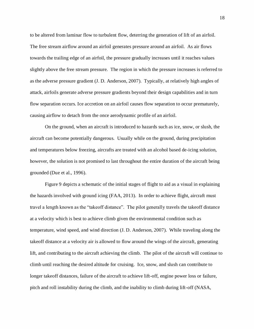
Figure 9 depicts a schematic of the initial stages of flight to aid as a visual in explaining
the hazards involved with ground icing (FAA, 2013). In order to achieve flight, aircraft must
travel a length known as the “takeoff distance”. The pilot generally travels the takeoff distance
at a velocity which is best to achieve climb given the environmental condition such as
temperature, wind speed, and wind direction (J. D. Anderson, 2007). While traveling along the
takeoff distance at a velocity air is allowed to flow around the wings of the aircraft, generating
lift, and contributing to the aircraft achieving the climb. The pilot of the aircraft will continue to
climb until reaching the desired altitude for cruising. Ice, snow, and slush can contribute to
longer takeoff distances, failure of the aircraft to achieve lift-off, engine power loss or failure,
pitch and roll instability during the climb, and the inability to climb during lift-off (NASA,
Page 33
19
2013a). The inabilities to climb during lift-off, longer takeoff distances, and pitch and roll
instability during the climb are all consequently due to turbulent flow around an airfoil.
Figure 9. Schematic of the initial stages of flight.
2.2.3. Performance degradation on propulsion systems due to icing. In regards to the
aircraft engine, ice can accrete on the aircraft propeller and compressor blades, causing undesired
vibrations among the blades, which can lead to failure and ingestion of the blades into the
aircraft propulsion system, resulting in internal damage of the aircraft (Mason et al., 2006;
Scavuzzo & Chu, 1987). Constant ingestion of supercooled droplets into an aircraft engine at a
relatively high frequency can extinguish the flame in the combustion chamber, causing “roll
back”. “Roll back” is a term used to describe an aircraft engine that has become irresponsive to
Page 34
20
any changes in thrust attempting to be made by the pilot, and loss of power (Mason et al., 2006;
Reehorst et al., 2010; Shastri et al., 1994).
Numerous simulations and predictor codes have been created in an effort to predict the
characteristics and end result of the complete formation of icing once it has began to adhere to
aircraft lifting surfaces. In addition to simulations and numerical predictor codes that attempt to
predict the formation of icing along aircraft structures, simulations and numerical predictor codes
have also been written to predict the magnitude of degradation that can occur based on ice
structures that have formed on airfoils. Extended information on the topic of simulations and
numerical predictor codes as they relate to ice formations and degradation on aircraft structures
due to icing is discussed in greater detail by Scavuzzo, Chu, Woods, et al. (1990), Scavuzzo,
Chu, and Kellacky (1990), Scavuzzo et al. (1994), Scavuzzo and Chu (1987), Harireche et al.
(2008), Labeas et al. (2006), and Thomas et al. (1996).
2.3. Anti-Icing and De-Icing Techniques
The primary goals of aircraft safety are to avoid, detect, and recover from any
degradation on an aircraft caused by icing conditions and environments (NASA, 2013b; Reehorst
et al., 2010). While detecting and recovering are both important in their own respects, the
present study will focus more towards avoiding any degradation on an aircraft caused by icing
conditions and environments. If aircraft icing can be avoided, then there will little, to no need, to
detect or recover from any degradation on an aircraft caused by icing.
De-icing techniques are often used to remove ice formations after they have adhered to a
surface, while anti-icing techniques are used to prevent ice from adhering from a surface. Anti-
icing techniques are used to avoid aircraft icing and de-icing techniques are used to recover from
degradation caused by ice accretion (Thomas et al., 1996). There are three types of anti-icing
Page 35
21
and de-icing techniques: chemical surfactants, mechanical systems, and thermal heating, each
with its own individual benefits and limitations (Geer & Scott, 1930; Scavuzzo & Chu, 1987;
Thomas et al., 1996).
2.3.1. Chemical surfactants. Chemical surfactants are used on aircrafts in the form of
surface treatments. These surface treatments directly affect the surface energy during contact
between the liquid droplets and the surface itself, resulting in surface properties capable of
generating hydrophilic and hydrophobic effects on droplets. A surface is considered to have
hydrophilic properties if it contributes to a liquid droplet wetting a surface, causing the liquid
droplet to display a contact angles below 90. In contrast, hydrophobic surfaces repel liquid
droplets, causing the liquid droplets to display contacts angles greater than 90. Surface energy
and the possible surface properties are explained in greater detail in Chapter 2.5.
The level of performance of a surfactant and whether the surfactant is capable of
achieving a desired objective depends on a variety of factors, such as the chemical compound of
the surfactant, environmental conditions which the surfactant is used, and even the rate at which
the surfactant is exposed to a given environmental condition. Using a combination of
siloxane(s), ethyl alcohol, ethyl sulfate, isopropyl alcohol, and fine-particle
polytetrafluoroethylene, NASA developed a hydrophobic coating, referred to as the Shuttle Ice
Liberation Coating, which they claim can reduce the adhesion of ice by as much as 90 percent
when compared to corresponding bare surfaces (Smith et al., 2008). Reich (1994) suggests that
chemicals possessing levels of silicone, such as siloxane, contribute to low adhesive strength in
the bond between icing and various materials used on aircraft.
Sakaue et al. (2008) developed a micelle polymer comprised of poly(N-
isopropylacrylamide) demonstrating that it is possible to utilize hydrophobic and hydrophilic
Page 36
22
coatings in a strategic manner and control how droplets interact with surfaces. Figure 10 depicts
a schematic of the micelle polymer and how the micelle polymer reacts to changes in
temperature. The micelle polymer features a reversible formation in its chemical makeup that
allows for the polymer to exhibit hydrophilic and hydrophobic properties with respect to
temperature.
Figure 10. Schematic of the how the micelle polymer interacts to changes in temperature
(Sakaue et al., 2008).
Figure 11 shows images of a liquid droplet interacting with an aluminum plate treated
with the micelle polymer. As temperature increased the micelle polymer treated aluminum
displayed hydrophobic surface properties and as temperature decreased, the micelle polymer
treated aluminum exhibited hydrophilic properties.
Page 37
23
Figure 11. Images of a liquid droplet interacting with an aluminum plate treated with the micelle
polymer (Sakaue et al., 2008).
Limitations develop in surface treatments when the repetitive cycle of applying and
removing ice or water is present, causing treatments to eventually lose their affect (Scavuzzo &
Chu, 1987). Figure 12 shows results of ice removal tests using elastic ceramic coatings and an
ice-phobic Du Pont coating (D. N. Anderson & Reich, 1997). The adhesive strength necessary
to cause debonding between the ice and substrates increase the number of ice removals
increased. According to Due et al. (1996), the repeated action of removing ice from a surface
coated with a surfactant, forms craters in the coatings, creating local areas where the film
thickness is dramatically reduced, leading to premature failure of the film. Cratering was found
Page 38
24
to be driven by surface tension gradients at the surface of coatings that cause surface movement
and removal of the underlying coating.
(a) (b)
Figure 12. Results of ice removal tests using (a) an elastic ceramic coating and (b) an ice-phobic
Du Pont coating.
Another factor that affects the efficiency of a chemical surfactant is the rate at which
precipitation impinges on a surface treatment. Figure 13 shows results from a test comparing
failure time of a glycol based freezing depressant to the average precipitation rate of ice (Due et
al., 1996). The failure time of a surfactant decreases as the rate of precipitation increases.
Depreciation of a surfactant is not limited to the repeated removal of ice however; water has also
been reported to depreciate the effectiveness of surfactants. According to Reich (1994), rain
erosion is a more severe process which not only destructs coatings, but at higher velocity and
Page 39
25
time, possesses the capabilities of eroding the substrate. The ideal chemical surfactants, in
regards to aircraft icing, must serve as an ice-phobic coating which can not only prevent ice from
adhering to the surface of an aircraft, but can also withstand rain erosion (Reich, 1994).
Figure 13. Results from a test comparing failure time of a glycol based freezing depressant to
the average precipitation rate of ice (Due et al., 1996).
2.3.2. Mechanical systems. De-icing techniques that require a power source to cause a
surface to become modified or deformed from its original shape is considered a mechanical
system (Thomas et al., 1996). The goal of mechanical systems is to modify an iced surface in a
manner that initiates cracking within the ice formation and cause debonding between the ice
formation and the surface of the aircraft, allowing for the aerodynamic forces acting on the
Page 40
26
aircraft to carry away the fractured ice. The three notable types of mechanical systems that have
been researched are: pneumatic boots, electromagnetic impulse, and electromagnetic expulsive
boots (Labeas et al., 2006; Scavuzzo, Chu, Woods, et al., 1990; Thomas et al., 1996; Venna et
al., 2007). Figure 14 is a schematic of a pneumatic boot used on commercial aircrafts. When
deactivated, the aircraft airfoil simply appears as a relatively normal airfoil, but when the
pneumatic boot is activated, the rubber boots equipped onto the airfoil inflate, deforming the
airfoil.
Figure 14. Schematic of a pneumatic boot used on commercial aircrafts.
Mechanical systems are strictly a de-icing technique, thus before the use of a mechanical
system can be utilized to its full potential, a particular amount of ice must adhere and accrete to
an aircraft structure (Landsburg, 2008; Thomas et al., 1996). The allowance of ice to accrete to
Page 41
27
the aircraft structure invites an increase in drag to the aircraft. Mechanical systems require a
power source, which is typically the aircraft battery. Some mechanical system power
requirements are more demanding than others, which can be more straining on the aircraft
battery. An even bigger issue arises when an aircraft equipped with mechanical systems is
presented with relatively high rates of icing (Thomas et al., 1996). High rates of icing may
require that a mechanical system operate continuously throughout flight which can lead to failure
of the mechanical system (Venna et al., 2007). In addition to the power consumption needed to
operate mechanical systems, some mechanical systems are physically heavy and add additional
weight to the aircraft (Venna et al., 2007).
2.3.3. Thermal heating. Thermal heating is the heating of the exterior of an aircraft by
means of either a power source, or redirecting heat generated from the aircraft engine (Thomas et
al., 1996). The heat generated by either heat source serves as both an anti-icing and de-icing
technique. Ice present on the aircraft structure prior to activating the thermal heating will melt,
and ice that impinges on a thermally heated surface will melt on contact. Miller, Lynch, and
Tate (2004) observed ice particles impinging on a thermally protected surface and concluded that
some particles bounced off of the heated surface, while others melted onto the heated surface
creating pools of cooled liquid. The supercooled liquid pools proceeded to freeze with the
impingement of subsequent ice particles. Miller, Lynch, and Tate (2004) also observed ice
particles cooled to -12.2C impact on hotwire water content sensors, which also resulted in
bouncing of the ice particles and the creation of pools of cooled liquid.
Heat must be applied along the entire aircraft structure for thermal heating to work well
in a cooled environment; else precipitation can melt, runback due to aerodynamic forces, and
refreeze at sections of the aircraft that lack proper heating (Geer & Scott, 1930). The rate at
Page 42
28
which precipitation impingement occurs is a factor that determines the efficiency of thermal
heating. At relatively high impingement rates, thermal heating sources can be cooled, causing
the thermal heat sources to lose their heating potential and can no longer contribute to preventing
ice from forming (Miller et al., 2004). Thermal heating also contributes to the corrosion of the
aircraft structure (Geer & Scott, 1930; Thomas et al., 1996). Corrosion of an aircraft structure
can lead to the premature failure of the aircraft.
2.4. Shear Strength of Ice on Aircraft Structures
Numerous shear stress tests were conducted throughout literature, each in their own
respective method, in effort to determine the shear strength necessary to cause debonding
between ice and substrates used to simulate aircraft structures (D. N. Anderson & Reich, 1997;
Fortin et al., 2010; Reich, 1994). Fortin et al. (2010) developed a centrifugal adhesion test in
which a beam was connected to a motor and programmed to rotate while supercooled droplets
impinged on its surface. Measuring the centrifugal force necessary to cause debonding between
the beam and impinging supercooled droplets, the adhesive strength of the impinging droplets on
aluminum was determined. Scavuzzo and Chu (1987) conducted shear stress tests at the Icing
Research Tunnel at the NASA Glenn Research Center in which two cylinders were utilized. One
cylinder was hollow with a larger inside diameter than the outside diameter of the second
cylinder. Ice was formed between the two cylinders, and a force was applied to the cylinders
until debonding occurred.
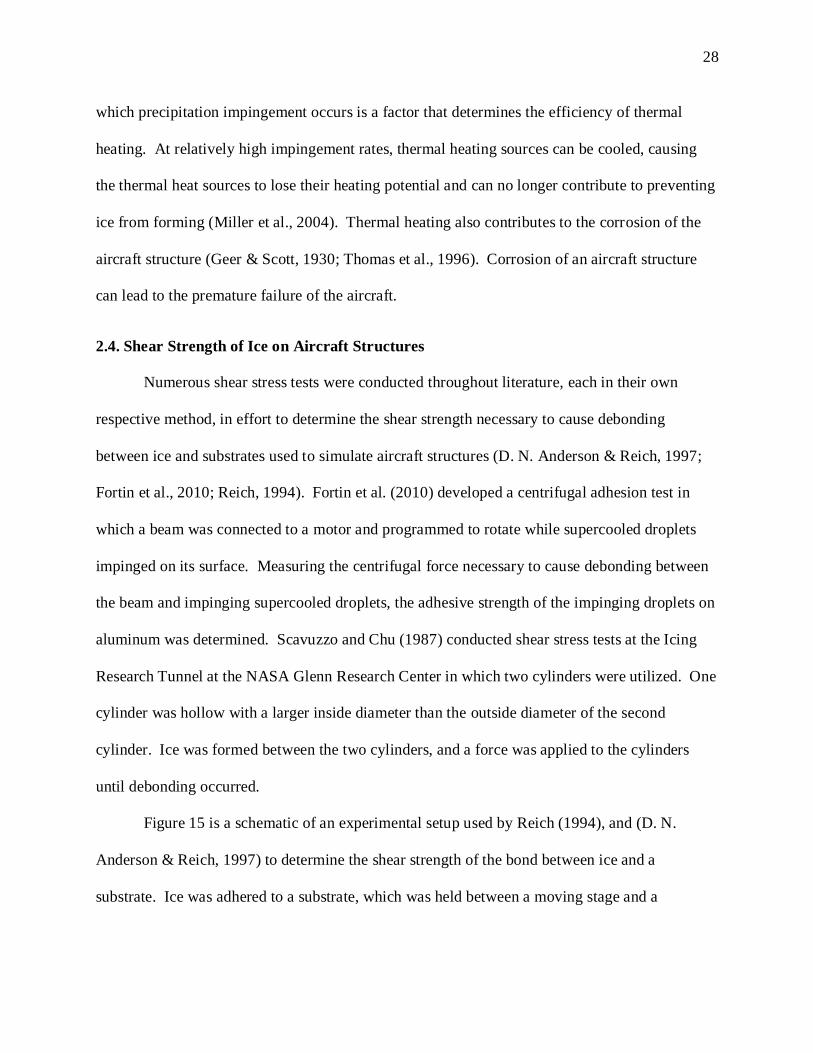
Figure 15 is a schematic of an experimental setup used by Reich (1994), and (D. N.
Anderson & Reich, 1997) to determine the shear strength of the bond between ice and a
substrate. Ice was adhered to a substrate, which was held between a moving stage and a
Page 43
29
stationary stage with a rough surface. Force was applied to the moving stage until debonding
occurred between the substrate and ice that has adhered to its surface.
Figure 15. Schematic of an experimental setup used by to determine the shear strength of the
bond between ice and a substrate (D. N. Anderson & Reich, 1997; Reich, 1994).
Table 1 lists the results of numerous ice adhesion tests conducted on various substrates
throughout literature (Fortin et al., 2010). According to Fortin et al. (2010) the highest adhesive
strength reported in literature for bare aluminum was 1.520 MPa, and the lowest reported
adhesive strength was 0.002 MPa. The large range and the variation in the reported adhesive
strength data throughout literature is due to a number of factors, such as different testing
conditions and experimental techniques, as well as surface finish, size, and type of substrate
being used, making it difficult to quantify the adhesive strength of ice with an absolute value
(Fortin et al., 2010). Refer to Fortin et al. (2010) for additional information, such as the sources
of the values in Table 1.
Page 44
30
Table 1
Results of ice adhesion tests conducted throughout literature (Fortin et al., 2010).
Substrate Adhesive Shear Stress (MPa)
Minimum Average Maximum
Aluminum N/A 1.520 N/A
Copper N/A 0.850 N/A
Polymers 1.030 N/A 1.170
Aluminum 0.067 N/A 0.400
Aluminum 0.002 N/A 0.110
Stainless Steel N/A 0.480 N/A
Aluminum 0.050 N/A 0.300
Aluminum 0.142 N/A 0.267 (smooth)
2.279 (rough)
In an effort to quantify the adhesive strength of ice on a substrate and the effectiveness of
coatings used on substrates against icing, Fortin et al. (2010) developed the adhesion reduction
factor (ARF). The ARF compares the average shear stress measured on coated substrates to the
average shear stress measured for bare substrates. The ARF is given by
(2.7)
A bare beam would have an ARF of one, while numbers less than one would indicate an increase
in the adhesive strength of ice on a substrate, and numbers larger than one would indicate a
decrease in the adhesive strength of ice.
Page 45
31
2.5. Shadowgraphing Visualization Technique
Shadowgraphing is a technique utilized in experimental fluid mechanics and heat transfer
as a tool for flow visualization by displaying refractions of light based on changes in fluid
density (Nepf, 2003; Panigrahi & Maralldhar, 2012). Figure 16 is a schematic of the general
experimental setup for the shadowgraphing technique (Panigrahi & Maralldhar, 2012). A light
source, a laser in the case of Figure 16, projects light through an object of interest, typically a
fluid, dispersing light throughout the object at a certain level of intensity. As an event occurs
that alters the density of the fluid, variations in the refractive index occur, deflecting or causing a
phase shift in the light passing through the fluid (Nepf, 2003). A screen is typically placed
opposite of the light source to capture the events occurring in the form of shadows, hence the
name “shadowgraphing”.
Figure 16. Schematic of the experimental setup for the shadowgraphing technique (Panigrahi &
Maralldhar, 2012).
Page 46
32
Figure 17 shows images of a heated water jet before and after the jet was activated using
the shadowgraphing technique (Panigrahi & Maralldhar, 2012). Initially, ring vortices formed,
progressively breaking down into turbulent flow, all of which are visible using shadowgraphing.
Figure 17. Images of a heated water jet (a) before and (b) after the jet was activated using the
shadowgraphing technique (Panigrahi & Maralldhar, 2012).
Shadowgraphing allows for events that typically cannot be seen with the human eye to be
visualized. Shadowgraphing and other flow visualization techniques are discussed in greater
detail by Nepf (2003), Panigrahi and Maralldhar (2012), Parthasarathy et al. (1985), Settles et al.
(2001), and Benson (2009) are recommended.
2.6. Definition of Wettability
Surface energy determines the type of interaction made by a liquid droplet when the
droplet comes into contact with a surface with respect to the solid, liquid, and vapor phases
present during the interaction Throughout literature, the accepted concept that is considered with
regards to surface energy is Young’s equation, which states that
Page 47
33
or
(2.8)
where , , and are the surface energy of the liquid-vapor, solid-liquid, and solid-vapor
interfaces respectively, and is the contact angle of the droplet. Figure 18 is a schematic of a
liquid droplet at equilibrium on a flat plate identifying the respective surface tension interfaces
(Liu & German, 1996). Equation 2.2 and Figure 18, assume that the resulting contact angle of
the liquid droplet depends strictly on the surface energy of the liquid-vapor, solid-liquid, and
solid-vapor interfaces. Young’s equation only holds true for droplets at equilibrium on a flat
plate. Young’s equation becomes modified when droplets are introduced to tilting plates
(Kawanishi et al., 1969; Krasovitski & Marmur, 2005; Pierce et al., 2007).
Figure 18. Schematic of a liquid droplet at equilibrium on a flat.
Characteristics of the interaction between a liquid droplet and a flat solid surface have
also been reported to become modified with the addition of external influences. The wetting
capabilities of a surface increase with the addition of heat, causing the sessile droplet to display
contact angles below 90 (De Coninck et al., 2000; De Gennes, 1985; Findenegg &
Herminghaus, 1997; Karmakov, 2000). The wetting capabilities of liquid droplets increase as
Page 48
34
heat increases, suggesting that there may be a correlation between heating and wetting (Aksay et
al., 1974; Bernardin et al., 1996; Boinovich & Emelyanenko, 2011; Hidaka et al., 2006; Janecek
& Nikolayev, 2013).
Figure 19 is an image of a sessile droplet on a substrate with voltage flowing throughout
the substrate (Kuo et al., 2003). In Figure 19, the droplet appears to be non-wetting, displaying a
contact angle above 90. The sessile droplet was induced with potassium chloride and set on a
substrate with 700 volts flowing throughout the substrate. It is suggested that these reactions
from the liquid droplet when introduced to electricity or heating is due to the fact that in its initial
state, the liquid-solid interface is not at chemical equilibrium. When the droplet is presented
with heat or electricity generated throughout the surface that the droplet is in contact with, the
liquid-solid interface reacts accordingly (Aksay et al., 1974; Bernardin et al., 1996).
Figure 19. Potassium chloride induced sessile droplet on a substrate subject to voltage (Kuo et
al., 2003).
Surfaces can be classified in five categories: hydrophobic, superhydrophobic,
hydrophilic, superhydrophilic, and ice-phobic (Kako et al., 2004; Sakaue et al., 2008; Salas-
Vernis et al., 2004; Zhang et al., 2010). The following sub-sections describe the classification of
surfaces.
Page 49
35
2.6.1. Hydrophobic and superhydrophobic surfaces. Surfaces are considered
hydrophobic if the surface causes droplets to display a contact angle greater than 90 and
superhydrophobic if the surface causes droplets to display a contact angle greater than 150.
Therefore, hydrophobic and superhydrophobic surfaces are considered non-wetting (Karmakov,
2000; Ma & Hill, 2006; Samaha & Gad-al-Hak, 2011). Hydrophobic surfaces can be produced
using either coatings, or through the development of micro- and nanostructures (Kako et al.,
2004; Ma & Hill, 2006; Samaha & Gad-al-Hak, 2011; Zhang et al., 2010). The effectiveness of
hydrophobic and superhydrophobic materials in regards to icing has varied throughout literature.
Zhang et al. (2010) developed superhydrophobic copper surfaces that they claimed had
“excellent” ice resistant characteristics. Farhadi et al. (2011) developed superhydrophobic
surfaces using micro- and nano-rough hydrophobic coatings and witnessed an increase in the
adhesive strength of ice. Farhadi et al. (2011) concluded that superhydrophobic surfaces may not
always be ice-phobic in the presence of humidity. The variance in results in the area of aircraft
icing as it pertains to hydrophobic surfaces is another example of the different testing conditions
and experimental techniques making it difficult to quantify the adhesive strength of ice with an
absolute value (Fortin et al., 2010).
2.6.2. Hydrophilic and superhydrophilic surfaces. Surfaces are considered hydrophilic
if the surface causes droplets to display a contact angle less than 90 and superhydrophobic if the
surface causes droplets to display a contact angle less than 30. Therefore, hydrophilic and
superhydrophilic surfaces are considered wetting (Bonn et al., 2009; De Coninck et al., 2000;
Findenegg & Herminghaus, 1997; Karmakov, 2000). Similar to hydrophobic surfaces,
hydrophilic surfaces can be produced using coatings, or through the development of micro- and
nanostructures (Kako et al., 2004; Salas-Vernis et al., 2004). Sakaue et al. (2008) developed a
Page 50
36
coating capable of exhibiting hydrophobic and hydrophilic characteristics with respect to
temperature. The surface of the substrate was hydrophobic as temperature increased and
hydrophilic as temperature decreased. Kako et al. (2004) demonstrated that the sliding behavior
of wet snow can be controlled by introducing hydrophilic channels to a superhydrophobic
surface. Throughout the literature review, hydrophilic surfaces have not been reported to reduce
ice adhesion.
The technique used to measure the contact angle of the sessile droplet shown in Figure 18
becomes inaccurate and impractical when measuring the contact angles of superhydrophilic
sessile droplets (Allen, 2003). The measurement technique in Figure 18 assumes the droplet is in
the shape of a spherical cap. However, the profile of a droplet is not in the shape of a spherical
cap at contact angles below 30. The method used to determine the contact angle of droplets that
do not form as spherical caps is by calculating the curvature of the droplet by numerically
solving the Laplace-Young equation (Allen, 2003). Allen (2003) developed much simpler
method to determine the contact angle of droplets that display contact angles below 30 knowing
only the volume and area of the droplet. The method reported by Allen (2003) is accurate only
for droplets less than 30.
2.6.3. Ice-phobic surfaces. Ice-phobicity does not particularly fall within the realms of
hydrophobic or hydrophilic (Freiberger & Lacks, 1961; Thomas et al., 1996). Ice-phobicity is
characterized by its ability to repel ice and not water, hence a surface that is characterized as
hydrophobic does not necessarily mean that same exact surface is ice-phobic (D. N. Anderson &
Reich, 1997; Thomas et al., 1996). Ice possesses different characteristics than water in terms of
density and phase. Techniques used to deter water, will not deter ice. Materials specifically
tailored to be ice-phobic have only been known to be produced in the form of coatings (Fortin et
Page 51
37
al., 2010; Freiberger & Lacks, 1961). Ice-phobic coatings lose their effectiveness with each
application and removal of icing (Due et al., 1996; Scavuzzo & Chu, 1987).
2.7. Literature Review Conclusion
Each anti-icing and de-icing technique developed comes with its own benefits and
limitations. No single anti-icing or de-icing technique reviewed throughout the literature review
reportedly completely deterred icing without any issues. The data collected throughout years of
literature on the adhesive strength of ice varies due to different testing conditions and
experimental techniques used by various authors making it difficult to assign an absolute value to
the adhesive strength of ice (Fortin et al., 2010). Reich (1994) commented that the ideal method
for deterring ice adhesion to aircraft structures should be both hydrophobic and ice-phobic.
Numerous studies have been, and are continuing to be, conducted to develop a material that
possesses a surface that is both hydrophobic and ice-phobic in the area of aircraft icing. There is
not much emphasis being put on the ice-phobic property. It should be noted that throughout the
literature review, hydrophilic surfaces have not been reported to reduce ice adhesion.
Page 52
38
CHAPTER 3
Methods and Materials
The following chapter describes the equipment, experimental setup, and procedures used
to meet the specific objectives of the present study. The adhesive strength tests were used to
determine the adhesive strength of the bond between ice that has formed and adhered to the
surfaces of bare and surfactant coated aluminum, stainless steel, copper, and polycarbonate
substrates at subcooled temperatures. The contact angles of sessile droplets interacting with bare
and treated substrates were measured to monitor changes in surface energy as it pertains to the
particular surfaces being observed. Observations of freezing of sessile droplets were conducted
to monitor the nucleation process of sessile droplets at subcooled temperatures and develop a rate
of freezing for the event. Finally, heat transfer lumped system analysis on the sessile droplet
exposed to subcooled conditions was done to develop an understanding of the cooling process of
a sessile droplet in a cooled environment analytically.
3.1. Determination of the Adhesive Strength of Ice on Various Substrates
Shear stress tests were performed to determine the adhesive strength of ice that has
adhered to various substrates chosen to simulate materials aircraft structures. The shear stress
tests were conducted on bare aluminum at -5, -10, -20, and -30C. Experiments were also
conducted on methoxymethylethoxypropanol, polymethylhydrosiloxane, and octylphenol
ethoxylate treated aluminum, stainless steel, copper, and polycarbonate substrates at -10C. An
additional experiment was conducted on bare aluminum, stainless steel, copper, and
polycarbonate substrates to determine a baseline of the adhesive strength of ice.
Page 53
39
All shear stress testing was conducted in an environmental chamber built in-house at
North Carolina Agricultural and Technical State University. Determining the size of the
substrates was important before any tests were conducted. Shear strength is given by
(3.1)
where is the applied force, and is the surface area at which the force is being applied. The
shear strength of the bond between the ice and various substrates was monitored with a PASCO
brand High Resolution Force Sensor, model number PS-2189. In order to determine the size of
the substrates, it was necessary to know the capabilities and limitations of the PASCO PasPort
High Resolution Force Sensor being used in this experiment and develop the substrates
accordingly. The force sensor senses forces up to 50 N and features a resolution of 0.002 N, a
maximum sampling rate of 1000 Hz (or 1000 samples per second), and dynamic variable over-
sampling, which aids in the reduction of measurement noise at low sample rates. According to
literature, the highest shear strength reported was 1.520 MPa, and the lowest 0.002 MPa, both on
aluminum substrates at -10C (Fortin et al., 2010). Given that information, the following
parameter regarding the area of the substrates used in this experiment was developed
or
In order for this experiment to be successful, given the limitations of the PASCO PasPort
High Resolution Force Sensor, the surface area of the substrates had to fall within the parameters
above. The substrates used in this experiment were 19.05 mm by 6.35 mm by 0.76 mm
aluminum, copper, steel, and polycarbonate strips. The surface area of the substrates used in this
Page 54
40
experiment was calculated to be 0.00024 m2. The thickness was neglected and it was
acknowledged that ice adhesion would occur on the front and back surfaces of the substrate.
Each material was chosen to simulate the materials used to fabricate aircrafts and the
particular size of the materials was determined to accommodate the capabilities of the PASCO
PasPort High Resolution Force Sensor being used. The PASCO PasPort High Resolution Force
Sensor was connected to a PASCO Xplorer GLX Handheld Datalogger. The PASCO Xplorer
GLX Handheld Datalogger directly collected, graphed, and allowed for analysis of collected data
without the use of a computer.
Fishing wire, with a maximum strength of up to 13.61 kg was used in this experiment to
link the substrates to the PASCO PasPort High Resolution Force Sensor. In order to
accommodate the fishing wire being used in this experiment, a 1.60 mm hole was drilled into
each substrate. Figure 20 shows an image of the configuration of the fishing wire used in the
present study. The Trilene fishing wire was tied through each substrate, secured by a knot, and a
loop was made at the opposite ends of the Trilene fishing wire, secured by another knot, to allow
the substrates to hang.
Figure 20. Configuration of the fishing wire used in the present study.
Page 55
41
Each substrate was wiped thoroughly using Sterahol, an ethanol, methanol, and isopropyl
alcohol solution, to rid the surfaces of the substrates of any contamination, as well as fingerprints
after the Trilene fishing wire was tied through the substrate and the loop was created at the
opposite end. Ridding the surfaces of the substrates of contamination was important to do before
placing the substrates into the environmental chamber because any sort of contamination, or
fingerprints, can affect the surface energy and adhesive strength between the ice and substrate.
As each substrate was cleansed, they were hung on a rod and allowed to air dry.
Figure 21 is a schematic of a substrate frozen within ice and the direction that force was
applied, all of which are within a modified ice tray. In order to successfully complete the shear
stress testing while ensuring that the substrates are never exposed to room temperature and
allowed to melt, an ice tray was modified with a polycarbonate cover. The polycarbonate cover
ensured that all ice that formed in the ice tray was held in its respective area in the event that the
ice dislodged from the tray. All tests were conducted within the environmental chamber.
Figure 21. Schematic of a substrate frozen within ice in a section of the modified ice tray.
Force
Page 56
42
The modified ice tray was also cleaned with Sterahol, while the substrates were drying.
The substrates were then placed into their own respective sections of the tray and distilled water
was poured into each section of the tray accordingly, covering approximately 6.35 mm of the
substrates. It was important to ensure that the water does not come into contact with the Trilene
fishing wire or the hole drilled to accommodate the fishing wire and be aware that water expands
as it freezes. Measurements would exceed the sensing capabilities of the PASCO PasPort High
Resolution Force Sensor if the Trilene fishing wire or the holes drilled in the substrates to
accommodate the fishing wire were frozen within the ice. Trials that exceeded the sensing
capabilities of the force sensor were discarded, and testing would be redone.
Prior to every test, before a load was applied, the button labeled “zero” on the PASCO
PasPort High Resolution Force Sensor was pressed to calibrate the data acquisition system.
Pressing the “zero” button would set the sensor to zero before any load was placed on the
PASCO PasPort High Resolution Force Sensor. Values measured while the force sensor was not
calibrated were discarded and the test was redone.
Figure 22 is an image of the experimental setup used to conduct the shear strength tests.
The PASCO PasPort High Resolution Force Sensor was equipped with a hook. The loop used to
originally hang the substrate was placed over the hook. The button on the PASCO Xplorer GLX
Handheld Datalogger with the “play” symbol was pressed after pressing the button labeled
“zero”. The button with the “play” symbol initiates the data logger and any force applied to the
force sensor would be measured and recorded by the force sensor. The data logger stores all of
the values measured internally until the user manually stops the data logger by pressing the
“play” button a second time. Force was manually applied until the substrate was dislodged from
Page 57
43
ice. As the load was applied to the PASCO PasPort High Resolution Force Sensor, the PASCO
Xplorer GLX Handheld Datalogger recorded the event.
Figure 22. Experimental setup for the shear strength tests.
Figure 23 is an image of ice that has been cracked due to the application of cyclic loading
while conducting a shear strength test. It was important to ensure that the force being applied
was constant and not done in a repetitive loading and unloading type cycle. Loading and
unloading the force would apply a cyclic load to the substrate, causing cracks to propagate within
the ice, weakening the integrity of the bond, and causing the PASCO Xplorer GLX Handheld
Page 58
44
Datalogger to log incorrect data. In the event of ice cracking, as shown in Figure 23, the data
measured was discarded.
Figure 23. Ice cracked due to the application of cyclic loading.
Measurements of the shear strength of ice was made on aluminum, stainless steel, copper,
and polycarbonate substrates, bare and treated with methoxymethylethoxypropanol,
polymethylhydrosiloxane, and octylphenol ethoxylate. The measured data was recorded in an
excel spread sheet. Fortin et al. (2010) commented that there is a large range and variation in the
reported adhesive strength data throughout literature due to factors, such as different testing
conditions and experimental techniques, as well as surface finish, size, and type of substrate
Page 59
45
being used, making it difficult to quantify the adhesive strength of ice with an absolute value. In
order to gauge the effectiveness of the data collected from the shear strength tests while using
surfactants, an adhesion reduction factor developed by Fortin et al. (2010) was used. Equation
2.1 was used to calculate the ARF. The ARF compares the average shear stress measured on
treated substrates to the average shear stress measured for bare substrates. A bare beam would
have an ARF of one, while numbers less than one would indicate an increase in the adhesive
strength of ice on a substrate, and numbers larger than one would indicate a decrease in the
adhesive strength of ice.
3.1.1. Environmental chamber. Shear strength tests were conducted in an
environmental chamber built in-house at North Carolina Agricultural and Technical State
University. Figure 24 is an image of the environmental chamber used to simulate subcooled
conditions. The structure of the environmental chamber was built using 80/20 Incorporated 2020
aluminum beams from their 10 series profile. The dimensions of the environmental chamber are
546.10 mm by 736.60 mm by 1485.90 mm. Housed within the chamber are two large custom
aluminum cooling plates built in-house, and between the larger cooling plates are four smaller
Lytron Total Thermal Solutions aluminum cooling plates (304.80 mm by 95.25 mm by 8.13
mm). Copper tubing (12.7 mm OD) purchased from McMaster-Carr was used throughout the
entire system to direct the flow of all working fluids. The aluminum beams that the
environmental chamber was comprised of were covered by 6.35 mm thick Lexan polycarbonate
sheeting. The polycarbonate sheeting was attached to the environmental chamber using sealed
by 50.8 mm wide silicone sealing strips. The exterior of the entire environmental chamber is
encased in reflective air-bubble wrap insulation, while the inside of the chamber is layered with
polystyrene foam panels.
Page 60
46
Figure 24. Environmental chamber used to simulate subcooled conditions.
Initially, the ambient temperature within the lab appeared to affect the temperature of the
working fluid by 3C. The fluctuation in temperature was possibly due to the lack of less than
perfect insulation around the copper tubing as well as the chamber itself. To deter this problem,
the insulation was observed and modifications were made to the insulation accordingly. Figure
25 shows the interior of the environmental chamber before and after polystyrene foam panels and
polystyrene spray foam were installed into the environmental chamber. The copper tubing
outside of the chamber was heavily insulated with foam pipe insulation and the inside of the
chamber was layered with polystyrene foam panels. The crevices around the foam panels were
sealed using polystyrene spray foam. Installing the polystyrene foam panels and polystyrene
spray foam enhanced the cooling capabilities of the environmental chamber by lowering the
Page 61
47
temperature inside the environmental chamber from -2C to -15C. The Polyscience Circulating
bath struggled to cool the working fluid to temperatures below -30C. The aforementioned lack
of insulation and the pump speed of the fluid were possible contributing factors affecting the lack
of cooling. Reducing the pump speed of the Polyscience Circulating bath contributed to cooling
the fluid by as much as -5C.
(a) (b)
Figure 25. Environmental chamber (a) before and (b) after installing polystyrene panels.
The environmental chamber utilizes a Remcor Industrial chiller (model CH-950) and a
Polyscience Circulating Bath (model PP15R-40). The working fluid throughout the entire
system is Dynalene HC, purchased from Polyscience under the consumer name: Polycool-HC50.
Dynalene HC is a colorless to light yellow, odorless, liquid capable of achieving temperatures as
high as 100C and as low as -50C. The chiller and bath combination was used because the
Page 62
48
Remcor Industrial chiller can only reach a minimum of -1.11C by itself and the cooling capacity
of the Polyscience Circulating Bath alone was not enough to cool the entire chamber to the
desired temperatures in a timely fashion. The Remcor Industrial chiller was initially activated
and allowed to cool the larger cooling plates and the air within the chamber to approximately -
1.11C. The Polyscience Circulating Bath was then activated to take on the remainder of the
cooling process and allowed to cool all of the cooling plates simultaneously, along with the air
within the chamber, to the desired temperatures.
Flow of the fluid throughout the chamber was controlled by two sets of valves which
allowed either the Remcor Industrial chiller or the Polyscience Circulating Bath to cool the entire
system alone, or both chillers to run and cool the system simultaneously. Through numerous
trials it was observed that achieving -40C using the chiller and bath combination alone was not
possible, and the minimum temperature possible was -15C. There are several reasons why this
holds to be true: less than perfect insulation, the absorption of energy from heat sources, flow
rate of the working fluid throughout the system, or even the configuration of the copper tubing
that the working fluid was transported through are just a few possibilities. In order to contribute
to the cooling process, 45.36 kg of solid carbon dioxide, dry ice, was placed at the bottom of the
chamber and allowed to sublimate within the chamber, further cooling the air within the chamber
to reach the desired temperature of -40C.
Heat sinks were attached to the Lytron Total Thermal Solutions cooling plates within the
environmental chamber to assist in the heat transfer process. Each heat sink was attached to a
Lytron cooling plate using Omega Engineering brand thermally conductive epoxy. Above each
heat sink was 0.85 ampere, 12 volt cooling fans. The cooling fans allowed the energy from the
cooling plates, as well as the heat sinks, to circulate within the chamber. The cooling fans were
Page 63
49
scavenged from decommissioned Gateway computers, model number E-2610S. The wiring of
the cooling fans were arranged in a parallel circuit and powered by a 12 volt power supply. The
cooling fans were activated while the Dynalene HC-50 flowed throughout the system.
Temperature was monitored using an IOTech Data Acquisition System, series number 6222.
The IOTech Data Acquisition System is a twelve channel, 12 port, 24 bit, thermocouple input
module device that connects directly to a PC via Ethernet cable.
3.1.2. Uncertainty analysis. Uncertainty analysis was done for the data measured in the
shear stress tests in order to determine the quality of the measured data. Uncertainty analysis
provides a range of which the true value is expected to fall within, while taking into account
measurement errors and random uncertainty. The true value of the shear stress necessary to
cause debonding between ice and the various substrates under the given conditions throughout
the shear stress tests are unknown, however, the data measured throughout the experiment
provides enough information to formulate a range of probable error. Since there were less than
30 values measured per data set, each data set was approached as a sample data set, thus the
sample mean, , sample variance, , and the sample standard deviation, , are respectively
defined by
(3.2)
(3.3)
(3.4)
Page 64
50
where N is the total number of samples, and is each individual measured value, where
. The sample mean value provides the most plausible estimate of the true mean
value, and the sample variance the most plausible measurement of the variation within a data set
(Figliola & Beasley, 2011). Experiments that require repeated measurements be taken under
fixed operating conditions inevitably encounter random error, which could be due to
measurement procedures and techniques, calibration of the equipment, resolution of the
equipment, and even the environmental conditions which measurements are being taken (Figliola
& Beasley, 2011). Random error is, in essence, the explanation for why data sets in experiments
that require multiple measurements are often scattered, as opposed to constant. Random
uncertainty provides an estimate of probable range of random error present within a data set.
Random uncertainty, , is defined by
(3.5)
where is the degrees of freedom in a data set, defined by , is the percent
probability, is a coverage factor used for finite data sets that represents a precision interval at
a given percent probability, and is the random standard uncertainty. The parameter can be
defined as
(3.6)
The solutions for were found using a distribution chart. Assuming a distribution
through a data set also assumes that there is a normal distribution of random error throughout the
data set. Equations 3.2 through 3.6 were applied in order to determine the random error
throughout the data at 95% probability after acquiring the data during the shear stress tests.
Page 65
51
3.2. Determination of Contact Angles
The contact angles of water on the various substrates were measured in order to monitor
any deviation that occurred between the surface energy between distilled water and the modified
substrates, compared to that of distilled water and the bare substrates. The contact angles of a
sessile droplet on bare, aluminum, stainless steel, copper, and polycarbonate substrates was
measured to develop a reference for the contact angles. The contact angles of
methoxymethylethoxypropanol, polymethylhydrosiloxane, and octylphenol ethoxylate treated,
aluminum, stainless steel, copper, and polycarbonate substrates was then measured. The
reference contact angles indicate any deviation of the contact angles measured on the treated
surfaces compared to the respective bare substrates.
The substrates used in this experiment were 25.40 mm by 25.40 mm aluminum, stainless
steel, copper, and polycarbonate square plates. As in the previous section, each substrate was
wiped thoroughly using Sterahol, an ethanol, methanol, and isopropyl alcohol solution, to rid the
surfaces of the substrates of any contamination, as well as fingerprints. Ridding the surfaces of
the substrates of contamination was important to do before observing the contact angles that the
distilled water displayed while interacting with the surfaces of the substrates because any sort of
contamination, or fingerprints could affect the surface energy and contact angles between the
distilled water and substrate.
Figure 26 shows a schematic of the experimental setup used to observe the contact angles
of droplets on the various substrates used throughout the present study. The substrates were then
allowed to air dry after being cleansed with Sterahol. A 0.10 mL droplet of distilled water was
then administered on the surface of the various substrates. The substrates were then placed in
Page 66
52
between a Cowboy Studio Tricolor backlight, and a Nikon D5100 Digital Camera. All images
were taken using the Nikon D5100 Digital Camera and saved as JPEG files on a local computer.
Figure 26. Schematic of the experimental setup used to observe the contact angles of droplets on
the substrates used throughout the present study.
Figure 27 shows a schematic of the method used to measure the contact angle of a droplet
relative to the surface of the substrates. The particular angle being measured was the angle
created between the liquid-solid interface and the solid-vapor interface of the droplet. All of the
images were then analyzed using ImageJ, a Java based image processing program developed by
the National Institute of Health (Ferreira & Rasband, 2013). ImageJ features an Angle tool that
was utilized to measure the contact angle of the droplets on the various substrates. The Angle
tool in ImageJ requires the user to draw two intersecting lines and measures the angle between
the lines. The JPEG files saved of the images of the droplets on the various substrates taken by
the Nikon D5100 Digital Camera were each individually imported into ImageJ and analyzed.
The plane that the liquid-solid interface was located on was identified in the JPEG files and the
Page 67
53
first line was drawn along that plane. The contact point of the droplet was then identified, and a
second line was drawn linearly along the surface of the droplet, intersecting with the contact
point of the droplet and the initial line drawn along the plane of the liquid-solid interface.
Figure 27. Schematic of the method used to measure the contact angle of a droplet.
The Measure tool was used in ImageJ in order to obtain an approximate value for the
angle between the intersecting lines after drawing the two intersecting lines. Wettability was
measured on bare, methoxymethylethoxypropanol, polymethylhydrosiloxane, and octylphenol
ethoxylate treated aluminum, stainless steel, copper, and polycarbonate substrates. When
applying the surface treatments to the substrates, similar procedures were followed as those used
to measure the contact angles of distilled water on the bare materials.
The substrates were first cleaned with Sterahol to rid the surfaces of any unwanted
contamination and fingerprints and allowed to air dry. The surfactants were then applied and
allowed to air dry once more before applying a 0.10 mL droplet of distilled water. The bare and
methoxymethylethoxypropanol treated substrates dried in approximately twenty minutes.
However, the polymethylhydrosiloxane and octylphenol ethoxylate surfactants possessed an oily
consistency and would not completely dry. Since neither the polymethylhydrosiloxane nor
octylphenol ethoxylate surfactants would air dry, the 0.10 mL droplet of distilled water was
Page 68
54
applied on top of the surfactants and the contact angle made during that interaction was
observed.
Surfaces that displayed superhydrophilic characteristics were measured using an
analytical solution for the determination of small contact angles of sessile droplets of arbitrary
size developed by Allen (2003) was used. The contact angle of sessile droplets less than 30 is
given by
(3.7)
where V is volume, and r is radius. Equation 3.7 is only valid if the contact angle is less than 30
and the bond number, , is less than one. Allen (2003) provided equations for bond numbers
greater than one, but warned that the equations for bond numbers greater than one are not as
accurate as Equation 3.7. The contact angle of superhydrophilic sessile droplets where 4, can
be approximated by
(3.8)
The contact angle of superhydrophilic sessile droplets where 25, can be approximated
by
(3.9)
The bond number is a measure of the relative effects of the gravitational and capillary
forces on the shape of the liquid surface. The bond number is expressed as
(3.10)
where r is the radius of the sessile droplet, and is the capillary length, which is given by
Page 69
55
(3.11)
where is surface tension, g is acceleration due to gravity, and and are the density of the
liquid and vapor phases, respectively. Throughout literature, the surface tension of water has
been reported to be 72 N/m2, gravity due to acceleration is 9.81 m/s
2, and the density of water
and air are accepted at 1000 kg/m3 and 1.20 kg/m
3 respectively (Cengel & Boles, 2008; Samaha
& Gad-al-Hak, 2011). Given the parameters of the variables necessary to determine the capillary
length, the capillary length can be calculated.
The radius of the sessile droplet, r, was determined by analyzing JPEG images captured
by the high speed camera using ImageJ. An image was opened in ImageJ, and initially, a scale
was set using the ‘set scale…’ feature in ImageJ based on any distinguishable, yet measureable,
feature in the image with respect to the number of pixels. The distinguishable feature chosen for
this experiment was the substrate that the droplet was placed on, which was measured to be
25.40 mm by 25.40 mm. Using the ‘straight line’ tool, a horizontal line was made across the
substrate to reference the width of the substrate. ‘Set scale…’ was found in the ImageJ toolbar
under the tab labeled ‘analyze’. The number of pixels within the line made earlier to reference
the width of the substrate was noted after choosing ‘set scale…’ in ImageJ. The known distance
and unit of the known distance were input into ImageJ.
A horizontal line was then made across the solid-liquid interface of the sessile droplet,
from end to end of the droplet profile. The “measure” feature was then utilized to determine the
length of the newly drawn line based on the scale that was previously set. The length that was
measured in ImageJ using the “measure” feature is the diameter of the sessile droplet. A vertical
line was drawn at the center of the sessile droplet using identical procedures to determine the
Page 70
56
height of the sessile droplet. The parameter was then calculated to determine the bond number
after determining the diameter of the sessile droplet. Once the bond number is determined,
Equation 3.7., 3.8, or 3.9 can then be applied accordingly. Equations 3.7-9 require the volume of
the sessile droplet to be known to determine the contact angle of sessile droplet. As mentioned
in Chapter 2.5.2., the profile of a superhydrophilic sessile droplet does not form in the shape of a
spherical cap. It is adequate to assume the shape of a spherical cap after determining the radius
and height of the sessile droplet. The volume, V, of a spherical cap is given by
(3.12)
The contact angle of the sessile droplet can be calculated after calculating the volume of the
superhydrophilic sessile droplet.
3.3. Visualization and Measurement of Freezing Rate of Sessile Droplets
A sessile droplet is a static droplet; therefore it is a steady droplet with no form of
velocity or acceleration. Observation of freezing a sessile droplet was made in order to
determine the nature and rate of the freezing process. Observations were made in an
environmental chamber built in-house at North Carolina Agricultural and Technical State
University. Figure 28 shows a schematic of the experimental setup used to observe the freezing
process of a sessile droplet. A 0.5 mL syringe was filled with distilled water and placed on a
chemistry test stand equipped with a clamp that was used as a syringe holder. The syringe was
first held upside down so that any air entrapped within the syringe would rise to the needle tip
and the syringe was relieved of any air before observing the freezing process of the sessile
droplet. Residual air was released from the syringe to avoid air bubbles from getting captured
within the sessile droplets being formed.
Page 71
57
Figure 28. Schematic of the experimental setup used to observe the freezing of a sessile droplet.
The tip of the syringe was removed and made flat as opposed to maintaining its original
acute tip. The needle tip was removed using a Dremel saw and the tip was smoothened using
360 grit sand paper. Removing the needle tip was done because the sharp tip on the syringe
diffracted light into the camera and appeared as a dark oval. The acute tip also affected the
orientation of the droplet itself; with the sharp tip, the droplet did not dispense from the syringe
as a symmetrical droplet but rather one that was lopsided. During this experiment it was
essential to ensure that the droplet was dispensed symmetrically and the tip was flat because the
orientation of the droplet (i.e. a lopsided droplet due to the syringe needle with the pointed tip)
affected how and where the droplet began to nucleate during the freezing process.
Figure 29 shows an image of the experimental setup used to visualize freezing sessile
droplets. The test stand was placed into the environmental chamber between the Fiber-Lite
Page 72
58
Illuminator System and a high speed camera after the syringe was clamped and secured to the
chemistry test stand. Images were taken in the chamber using a high-speed camera. The high
speed camera had capabilities of recording up to 50,000 frames per second and the software
associated with the high speed camera was the Photon FASTCAM Viewer (PFV) for High-speed
Digital Imaging, version .323.
Figure 29. Experimental setup used to visualize freezing sessile droplets.
The interface for the PFV software was used to specify the settings for the high speed
camera prior to operating the camera. The general settings used while recording video for this
experiment with the high speed camera was a resolution of 1024 by 1024 and a frame rate of 250
frames per second. The high speed camera records a total of 5457 frames, each frame occupying
a frame of time. The higher the frame rate the smaller the window of time the user was allowed
to record and vice versa. At smaller frame rates, the user is allowed to record a larger window of
Page 73
59
time, but risks missing important events due to the lack of frames being recorded. A frame rate
setting of 250 frames per second was optimal for this experiment since it captured enough frames
to reveal what occurred throughout the freezing process, as well as allowing an efficient time
window.
Icing can occur within a matter of milliseconds, and what makes icing even more
inconvenient is the unpredictability of when the sessile droplet would begin to nucleate. The
trigger mode of the high speed camera was changed to ‘end mode’ to account for the
unpredictability of nucleation. In ‘end mode’ the high speed camera continuously records until
the user manually stops recording an event. However, while in ‘end mode’ when the high speed
camera reaches the maximum number of frames it can record, the high speed camera proceeds to
continuously dump the earliest images, which are temporarily saved internally within the high
speed camera, to make room for the newest images. The time window allowed for the user to
manually stop recording the images taken by the high speed camera correlates with the frame
rate chosen, and as previously mentioned, the higher the frame rate the smaller the window of
time the user is allowed to record, and vice versa.
A Fiber-Lite Illuminator System was used as the backlight while recording images with
the high speed camera within the chamber. The Fiber-Lite Illuminator System uses fiber optics
as a method of absorbing heat and producing a high intensity cold light. The fiber optic backlight
does not radiate heat into the chamber, while other types of lighting sources generally operate as
hot lights and become heating sources. The fiber optics in the Fiber-Lite Illuminator System was
housed in a gooseneck light pipe which allowed for versatility in the positioning of the lighting.
The ability of having versatility in the positioning of the lighting was important because when
positioning the light behind the sessile droplet, the light had to be repeatedly positioned where
Page 74
60
there was little to no inequalities in the lighting throughout the droplet. The inequalities would
typically show in the images being recorded by the high speed camera as dark spots around the
edges of the droplet. The goal behind adjusting the Fiber-Lite Illuminator System was to
eliminate the majority of the dark spots within the droplet that was being captured by the high
speed camera, leaving only a faint outline of the sessile droplet.
The test stand was placed into the environmental chamber between the Fiber-Lite
Illuminator System and a high speed camera after the syringe was clamped and secured to the
chemistry test stand. The proper settings were applied to the high speed camera. The Fiber-Lite
Illuminator System was adjusted to the desired position. The high speed camera was activated
and images were captured. The camera was manually stopped after the sessile droplet was
completely frozen. The freezing process was monitored using a shadowgraphing technique.
Shadowgraphing is an optical tactic that reveals non-uniformities throughout events that would
regularly appear transparent via refractions in the lighting. The outline of the droplet with light
being generated from the Fiber-Lite Illuminator System shining through the droplet should be
visible if configured correctly. As freezing occurred, the droplet began to darken until it was
almost completely black, and most of the light generated by the Fiber-Lite Illuminator System
was no longer seen through the droplet. However, if configured incorrectly, the light will not be
diffracted from the high speed camera in a manner that would reveal the solidification process;
instead the outline of the droplet will remain as an outline throughout the freezing process.
The frames that were recorded by the high speed camera was viewed and edited to
remove any useless and repetitive frames that were recorded, minimizing the size of the files that
were to be saved. All of the frames recorded by the high speed camera were saved as both AVI
and JPEG files. The AVI file offered a visual of the entire event in real time as it occurred, while
Page 75
61
the JPEG files offered frame by frame visuals of the event. The JPEG files become helpful when
observing the transitions made by the sessile droplet during the freezing process with respect to
time, which is impractical when viewing the AVI file. Each individual JPEG possesses
important information such as the frame rate and resolution that was used while recording the
image and the specific time of occurrence of the event within that frame. The time elapsed for
the sessile droplet to completely solidify was found using the time given in each frame.
The JPEG images were reviewed and several were chosen to illustrate the nature of the
occurrence of the freezing process of a sessile droplet. Images chosen were analyzed using
ImageJ, a Java based image processing program developed by the National Institute of Health.
The images were each individually opened and analyzed in ImageJ using identical procedures.
Initially, a scale was set using the ‘set scale…’ feature in ImageJ based on any distinguishable,
yet measureable, feature in the image with respect to the number of pixels within the
distinguished feature. The feature chosen for this experiment was the syringe needle. Using the
‘straight line’ tool, a horizontal line was made across the syringe needle to reference the diameter
of the needle. The syringe needle was measured with a Venier Caliper, and was found to be
in diameter. ‘Set scale…’ was found in the ImageJ toolbar under the tab labeled
‘analyze’. The number of pixels within the line made earlier to reference the diameter of the
syringe needle was noted after choosing ‘set scale…’in ImageJ. The known distance and unit of
the known distance were input into ImageJ.
A square was then made around the area of interest using the “rectangular” tool and the
“clear outside” feature was then applied to the image, isolating the droplet from the original
image. Next, the image was converted to black and white by adjusting the threshold of the
original image. The image was converted to black and white by utilizing the “threshold” feature
Page 76
62
in ImageJ. In the “threshold” interface, a drop down menu that represents the extremities of the
color schemes used in ImageJ was changed from “red” to “B&W” which represents black and
white. Converting the color scheme of the images to black and white allowed the solid content
of the droplet, which appeared as black, to be clearly distinguished from the liquid content
remaining within the droplet, which appeared as white. The “analyze particle” feature was then
used to analyze the area of the liquid and solid content throughout the droplet. The “analyze
particle” feature demonstrated a limitation in that the feature could only identify particles in their
entirety. The “analyze particle” feature could not identify droplets within droplets. In the case
of a droplet being encased within another droplet, ImageJ tended to only identify the properties
of the black area within the images. For example, the images that consisted of a partially
solidified droplet, meaning there was a visible distinction between the solid and liquid content of
the droplet recognized by ImageJ, could only be analyzed as a complete solid droplet using the
“analyze particle” feature.
In order to maneuver around that particular limitation, the “analyze particle” feature was
first used to find the area of the entire droplet. The black and white color scheme of the droplet
was inverted, causing solids to appear white and liquids to appear black. The area was then
found solely for the liquid content remaining within the droplet. The solid content of the droplet
was found by taking the difference between the area of the entire droplet and the area of the
liquid content within the droplet. The solid and liquid content of the droplet was converted into
percentages using Equations 3.10 and 3.11 respectively after the areas for the solid and liquid
was determined.
(3.10)
Page 77
63
(3.11)
ImageJ assumes all images uploaded into the program are two dimensional images. In
order to account for that assumption being applied to the spherical sessile droplets observed in
the present study, the radius of the liquid content was measured. The radius of the liquid content
of the sessile droplets was determined from the area of the liquid using Equation 3.12.
(3.12)
The volume of the liquid was determined using Equation 3.13 after determining the
radius of the liquid content remaining in the sessile droplet. Knowing the volume, volumetric
freezing rate was then determined using Equation 3.14. The volumetric freeze rate provides a
rate at which freezing is occurring in terms of volume with respect to time. The total freeze time
provides the time elapsed for freezing to occur from the onset of freezing until the droplet has
completely solidified. The total freeze time of the freezing process was determined using
Equation 3.15.
(3.13)
(3.14)
(3.15)
In addition to visualizing freezing of sessile droplets dispensed from a syringe, droplets
were visualized freezing in subcooled silicone oil. Figure 30 is a schematic of the experiment
setup used to visualize freezing in silicone oil. A polycarbonate test tube was filled with
supercooled silicone oil and placed between a Cowboy Studio Tricolor backlight and high speed
Page 78
64
camera. The high speed camera was set at a resolution of 1024 by 1024 and a frame rate of 125
frames per second. Water droplets were dispensed into the supercooled silicone oil using a 0.5
mL syringe. Water droplets were visualized freezing in supercooled silicone oil in an effort to
determine a homogeneous nucleation freezing process.
Figure 30. Schematic of the experiment setup used to visualize freezing in silicone oil.
3.4. Heat Transfer Lumped System Analysis
Lumped system analysis was done in order to determine the rate of heat transfer of the
sessile droplet when placed in the environmental chamber numerically. Figure 31 is a schematic
of the condition that were simulated using the heat transfer lumped system analysis. A spherical
liquid droplet was exposed to a subcooled surrounding temperature, T. The temperature
distribution around the spherical droplet is assumed to be equal. As the surrounding temperature
Page 79
65
begins to influence the temperature of the droplet by means of convection, heat flux is loss. The
heat transfer process between the droplet and the surrounding temperature is dependent on the
thermal conductivity, k, density, , and specific heat, c of the liquid droplet.
Figure 31. Schematic of the condition simulated using heat transfer lumped system analysis.
Prior to conducting the heat transfer lumped system analysis, an experiment was
conducted to measure the convective heat transfer coefficient, h. Figure 32 is a schematic of the
experimental setup used to measure the convective heat transfer coefficient. A heater cartridge
connected to a power supply was placed into the subcooled environmental chamber. The power
supply allowed for the input of a known voltage and current to be applied to the heater cartridge.
Page 80
66
The surrounding temperature and the temperature of the heater cartridge was monitored by a data
acquisition system equipped with K-type thermocouples.
Figure 32. Schematic of the experimental setup used to measure the convective heat transfer
coefficient.
The environmental chamber was subcooled to -40C. The heater cartridge was used to
introduce the subcooled conditions within the environmental chamber with heat flux in order to
meet the conditions of Newton’s Law of Cooling, which states that
(3.16)
Page 81
67
where q is the heat flux, To is the temperature of the heater cartridge, and T is the constant
temperature within the environmental chamber. The heater cartridge was connected to a 6030A
System Power Supply, which was set to 5.0 volts and 1.0 amperes, and placed inside the
environmental chamber where it was then allowed to heat. The temperature of the heater
cartridge was monitored using an IOTech Data Acquisition System, series number 6222. The
temperature of the heater cartridge was observed until the temperature plateaued, which was
rounded to the nearest whole number and recorded. The primary component of the heater
cartridges that were contributing heat into the environmental chamber were four cylindrical
prongs, each of identical size. The 6030A System Power Supply was then powered off, and the
heater cartridge was removed from the 6030A System Power Supply and allowed to cool to
room temperature. The diameter and height of cylindrical prongs were measured using a Vernier
caliper and found to be 0.00635 m and 0.060 m, respectively. Knowing the diameter, d, and in
turn, the radius, r, and the height, h, of the cylindrical prongs, the area of the prongs, , was
found using the following equation,
(3.17)
Heat flux is watts per unit area, thus knowing the area of each prong and the voltage and
current that the system was operating under, it was possible to calculate heat flux using this
experimental setup. Heat flux was calculated using the following equation,
(3.18)
where i is current, V is voltage, and P represents power, which is the product of the current
multiplied by the voltage. Recalling Equation 3.16, after calculating the heat flux, Newton’s
Law of Cooling can then be applied to determine the convective heat transfer coefficient, h, of
the operating system within the environmental chamber, with h being the only unknown.
Page 82
68
Knowing the convective heat transfer coefficient, the Biot number for the sessile droplet inside
of the environmental chamber was then calculated. The Biot number numerically describes
temperature distribution throughout a system during transient heating or cooling processes,
assuming that the temperature distribution is uniform throughout the system. Lumped system
analysis can only be performed on a system if the Biot number of the system is less than 0.1.
The Biot number, Bi, is given by
(3.19)
where V is volume, As is the surface area of the sessile droplet, k is the thermal conductivity
coefficient, and Lc is the characteristic length. The thermal conductivity of water was found in
literature to be 0.613 W/mK at room temperature (Cengel & Boles, 2008; Gieck & Gieck,
2006). The sessile droplet was assumed to be a sphere, thus the characteristic length was given
by
(3.20)
The radius of the sessile droplet, r, was determined by analyzing JPEG images captured
by the high speed camera using ImageJ. Similarly to the experiment in section 3.3, an image was
opened in ImageJ and a scale was set using the ‘set scale…’ feature based on any
distinguishable, yet measureable, feature in the image with respect to the number of pixels within
the distinguished feature. The feature chosen for this experiment was the syringe needle. Using
the ‘straight line’ tool, a horizontal line was made across the syringe needle to reference the
diameter of the needle. The syringe needle was measured with a Venier Caliper, and was found
to be 1.0 mm in diameter. ‘Set scale…’ was found in the ImageJ toolbar under the tab labeled
Page 83
69
‘analyze’. The number of pixels within the line made earlier to reference the diameter of the
syringe needle was noted after choosing ‘set scale…’ in ImageJ. The known distance and unit of
the known distance were input into ImageJ.
Another horizontal line was then made across the widest portion of the sessile droplet,
which was typically located at the midsection of the sessile droplet. The “measure” feature was
then utilized to determine the length of the newly drawn line based on the scale that was
previously set. The length that was measured by ImageJ using the “measure” feature served as
the diameter of the sessile droplet. The radius of the sessile droplet was then used to obtain the
characteristic length of the sessile droplet. The Biot number was then calculated using Equation
3.19. Once confirmed that the Biot number of the system was less than 0.1, the Fourier number
was calculated. The Fourier number describes the magnitude of the effects of the degree of
cooling or heating within a system, and was obtained using the following equation
(3.21)
where is thermal diffusivity and t is time. Time, t, was obtained from the images taken by the
high speed camera. Each frame recorded by the high speed camera was marked with a time
stamp which indicated when a particular event occur based on the frame rate at which the images
were taken. Thermal diffusivity is a thermophysical property the represents the rate at which
heat is capable of diffusing through a medium. The larger the thermal diffusivity, the faster heat
will diffuse through a medium. The thermal diffusivity is given by
(3.22)
where is the density and c is the specific heat. The density and specific heat of water has been
reported throughout literature to be 1000 kg/m3 and 4.22 kJ/kgK, respectively (Cengel & Boles,
Page 84
70
2008). The Fourier number can then be calculated using Equation 3.21 after calculating the
thermal diffusivity. A heat transfer lumped system analysis can then be performed by applying
the following equation,
(3.23)
where T is the temperature within the environmental chamber, Ti is the initial temperature of the
droplet, which in case was room temperature, T(t) is temperature with respect to time and t is
time. Time, t, was obtained from the images taken by the high speed camera. Each frame
recorded by the high speed camera was marked with a time stamp which indicated when a
particular event occurred based on the frame rate at which the images were taken. T(t) was the
only unknown term in Equation 3.23 and the term of interest in this analysis. Therefore Equation
3.23 was rewritten as
(3.24)
All of the terms in Equation 3.24 were constant, with the exception of time, t, and T(t)
which is a function of time. Equation 3.24 was written, solved and plotted using MATLAB, a
computer programming language used for numerical computing.
Table 2 presents the results from a temporal independent study performed on the
MATLAB code written for the heat transfer lumped system analysis. A temporal independent
study was performed in order to determine an optimum time step to operate the heat transfer
lumped system code in which the time step did not have a significant effect on the results. The
temporal independent study was performed at time steps of 10, 1, 0.1, 0.01, and 0.001 seconds.
Time for the system to reach -40C was observed to increase from 3.48 to 3.486 seconds
Page 85
71
between time steps of 0.01 and 0.001, respectively, thus 0.01 was the time step used in the
present study to conduct the lumped system analysis.
Table 2
Results of a temporal independent study performed on the code written for heat transfer lumped
system analysis.
t, s Time, s (to reach -40C)
10 10
1 4
0.1 3.50
0.01 3.48
0.001 3.486
Page 86
72
CHAPTER 4
Results
The following chapter will begin by presenting the results of the shear stress tests. The
shear stress tests were conducted on bare aluminum at -5, -10, -20, and -30C. Experiments were
also conducted on methoxymethylethoxypropanol, polymethylhydrosiloxane, and octylphenol
ethoxylate treated aluminum, stainless steel, copper, and polycarbonate substrates at -10C. An
additional experiment was conducted on bare aluminum, stainless steel, copper, and
polycarbonate substrates to determine a baseline of the adhesive strength of ice in the present
study. The current chapter will then present the results obtained from measuring the contact
angles of sessile droplets on bare and methoxymethylethoxypropanol, polymethylhydrosiloxane,
and octylphenol ethoxylate treated aluminum, stainless steel, copper, and polycarbonate
substrates. Next, the results of the images taken using shadowgraphing will be presented.
Finally, the results of the heat transfer lumped system analysis on the sessile droplet exposed to
subcooled conditions will be presented and compared to the results observed while using
shadowgraphing to view freezing in a sessile droplet and the rate at which freezing occurs.
4.1. Adhesive Strength of Ice on Various Substrates at Subcooled Temperatures
Shear stress tests were conducted to determine the adhesive strength of ice to substrates
chosen to simulate materials used on aircraft structures. Prior to testing the adhesive strength of
ice to methoxymethylethoxypropanol, polymethylhydrosiloxane, and octylphenol ethoxylate
treated aluminum, stainless steel, copper, and polycarbonate substrates, shear stress tested were
conducted on bare aluminum at -5, -10, -20, and -30C to determine whether temperature had an
effect on the adhesive strength of ice. The raw data measured for all of the shear stress tests
conducted in the present study are presented in the appendices. Figure 33 and Table A-1
Page 87
73
displays the results from the shear stress tests conducted on bare aluminum at -5, -10, -20, and -
30C. 30 trials were conducted at each temperature. As Fortin et al. (2010) stated, there is a
large range and variation in the reported adhesive strength data throughout literature making it
difficult to quantify the adhesive strength of ice with an absolute value, and the data presented in
Figure 33 and Table A-1 are nothing short of that statement. The data measured throughout the
current adhesive strength test and other variations of the experiment in the present study were
scattered. There was never any certain absolute value that could be assigned to represent the
adhesive strength of ice.
Figure 33. Adhesive strength of ice on bare aluminum at -5, -10, -20, and -30C.
0.00
0.05
0.10
0.15
0.20
0.25
0.30
0.35
0.40
0 5 10 15 20 25 30
Sh
ea
r S
tress
(M
Pa
)
Trials
-5 deg. C -10 deg. C -20 deg. C -30 deg. C
Page 88
74
Table 3 presents a summary of the average, standard deviation, and uncertainty analysis
of the data collected from the adhesive strength tests conducted on bare aluminum at various
subcooled temperatures. Table 3 reveals that temperature had very little effect on the average
adhesive strength of ice to aluminum substrates. The average adhesive strength was measured to
be 0.2150.031 MPa at -5C. The average adhesive strength of ice measured at -10C was
0.1840.031 MPa, decreasing compared to the average adhesive strength measured at -5C. The
average adhesive strength at -20C was measured to be 0.2150.041 MPa, increasing compared
to the 0.1840.031 MPa measured at -10C. The average adhesive strength was measured to be
0.2020.035 MPa at -30C, decreasing compared to the 0.2130.041 MPa measured at -20C.
Table 3
Summary of the adhesive strength of ice on bare aluminum at -5, -10, -20, and -30C.
Temperature
Average Shear
Stress (MPa)
Standard
Deviation
Random Standard
Uncertainty
Random Uncertainty
(95% Confidence)
-5C 0.215 0.070 0.013 0.031
-10C 0.184 0.070 0.013 0.031
-20C 0.213 0.094 0.017 0.041
-30C 0.202 0.08 0.015 0.035
Though the data in Figure 33 and Table A-1 appear scattered, there was very little
deviation in the in the average adhesive strength of the data collected at -5, -10, -20, and -30C,
which can be observed in Table 3. The average adhesive strength of ice measured on aluminum
Page 89
75
at -5, -10, -20, and -30C, suggests that the adhesive strength of ice is not dependent on
temperature.
Once it was determined that the adhesive strength of ice was not dependent on
temperature, the remaining shear stress tests were conducted at -10C, and instead of 30 trials,
eight trials were performed for each substrate and surface modification. Figure 34 shows the
average adhesive strength of the shear stress of ice on bare stainless steel, copper, and
polycarbonate substrates at -10C from the data presented in Table A-2. The results suggest that
ice measured the highest adhesive strengths on the copper substrates, and the lowest adhesive
strengths on the aluminum substrates.
Figure 34. Average adhesive strength of ice on bare substrates.
0.00
0.10
0.20
0.30
0.40
0.50
0.60
0.70
0.80
Aluminum Stainless Steel Copper Polycarbonate
Av
erag
e A
dh
esi
ve S
tren
gth
(M
Pa)
Material
Page 90
76
Table 4 presents the average, standard deviation, and uncertainty analysis of the data
shown in Table A-2. The values in Table 4 correspond with the data measured from the adhesive
strength tests conducted on bare aluminum, copper, stainless steel, and polycarbonate at -10C.
The results reveal that the average adhesive strength of ice was most significant on bare copper
than it was on aluminum, stainless steel, and polycarbonate. Table 4 also reveals that there was a
relatively larger variation in the adhesive strength of ice on copper, which was determined from
the standard deviation calculated. The average adhesive strength of stainless steel was measured
to be 0.4410.035 MPa, which agrees well with the average adhesive strength of 0.480 MPa
reported by Jellinek et al. (1981). The average adhesive strength of ice on bare aluminum was
measured to be the least of the materials used throughout the present study.
Table 4
Summary of the adhesive strength of ice on bare substrates.
Material
Average Shear
Stress (MPa)
Standard
Deviation
Random Standard
Uncertainty
Random Uncertainty
(95% Confidence)
Aluminum 0.184 0.069 0.013 0.031
Stainless Steel 0.441 0.041 0.014 0.035
Copper 0.648 0.182 0.064 0.156
Polycarbonate 0.600 0.094 0.033 0.080
Figure 35 presents the average adhesive strength of ice on methoxymethylethoxypropanol
treated aluminum, stainless steel, copper, and polycarbonate substrates at -10C from the data
shown in Table A-3. Methoxymethylethoxypropanol is a chemical that is advertised in industry
to operate as water repellant. Figure 35 suggests that the methoxymethylethoxypropanol
Page 91
77
treatment increased the adhesive strength of ice on all of the substrates observed in the present
study. Similar to the results measured on the adhesive strength of ice to the bare substrates,
copper was measured to demonstrate the highest average adhesive strength after being treated
with methoxymethylethoxypropanol. Aluminum demonstrated the lowest average adhesive
strength after being treated with methoxymethylethoxypropanol.
Figure 35. Average adhesive strength of ice on methoxymethylethoxypropanol treated
substrates.
0.00
0.20
0.40
0.60
0.80
1.00
1.20
1.40
1.60
Aluminum Stainless Steel Copper Polycarbonate
Av
erag
e A
dh
esi
ve S
tren
gth
(M
Pa)
Material
Bare Methoxymethylethoxypropanol Treated
Page 92
78
Table 5 presents the average, standard deviation, and uncertainty analysis of the data
presented in Table A-3. The values in Table 5 correspond with the data measured from the
adhesive strength tests conducted on methoxymethylethoxypropanol treated substrates.
Aluminum was measured to have the lowest adhesive strength values compared to the remaining
substrates observed in the present study, while copper was measured to have the highest adhesive
strength values. Aluminum measured an average adhesive strength of 0.4870.069 MPa, while
the stainless steel, copper, and polycarbonate substrates measured average adhesive strengths of
1.0780.058, 1.2360.060, and 1.1210.135 MPa respectively.
Table 5
Summary of the adhesive strength of ice on methoxymethylethoxypropanol treated substrates.
Material
Average Shear
Stress (MPa)
Standard
Deviation
Random Standard
Uncertainty
Random Uncertainty
(95% Confidence)
Aluminum 0.487 0.081 0.029 0.069
Stainless Steel 1.078 0.067 0.024 0.058
Copper 1.236 0.070 0.025 0.060
Polycarbonate 1.121 0.158 0.056 0.135
Table 6 presents the adhesion reduction factor, ARF, and percent difference of the
average adhesive strengths measured on methoxymethylethoxypropanol treated substrates. The
ARF compares the average shear stress measured on treated substrates to the average shear stress
measured for bare substrates. A bare beam would have an ARF of one, while numbers less than
one would indicate an increase in the adhesive strength of ice on a substrate, and numbers larger
than one would indicate a decrease in the adhesive strength of ice. Table 6 reveals that the
Page 93
79
methoxymethylethoxypropanol treatment increased the adhesive strength of ice on all of the
substrates observed in the present study. The adhesive strength of ice to aluminum, stainless
steel, copper, and polycarbonate increased by 165.60%, 144.60%, 90.77%, and 86.80%
respectively. From the results in Table 6, it can be concluded that
methoxymethylethoxypropanol, a chemical advertised to repel water, does not necessarily repel
icing.
Table 6
ARF and percent difference of methoxymethylethoxypropanol treated substrates.
Methoxymethylethoxypropanol
Material Average Shear Strength ARF Percent Difference (%)
Aluminum 0.487 0.38 165.60
Stainless Steel 1.078 0.41 144.60
Copper 1.236 0.52 90.77
Polycarbonate 1.121 0.54 86.80
Figure 36 presents the average adhesive strength of ice on polymethylhydrosiloxane
treated aluminum, stainless steel, copper, and polycarbonate substrates at -10C from the data
presented in Table A-4. Figure 36 reveals that the polymethylhydrosiloxane treatment increased
the adhesive strength of ice on the copper substrates the most compared to the remaining
substrates observed in the present study. The adhesive strength of ice measured on the metallic
substrates was measured to have increased. However, the adhesive strength of ice was reduced
on polymethylhydrosiloxane treated polycarbonate. Similar to the results measured on the
adhesive strength of ice to the bare substrates, copper was measured to demonstrate the highest
Page 94
80
average adhesive strength after being treated with polymethylhydrosiloxane. Aluminum
demonstrated the lowest average adhesive strength after being treated with
polymethylhydrosiloxane.
Figure 36. Average adhesive strength of ice on polymethylhydrosiloxane treated substrates.
Table 7 presents the average, standard deviation, and uncertainty analysis of the data
presented in Table A-4. The results reveal the average adhesive strength of ice on the
polymethylhydrosiloxane treated copper was greatest compared to the remaining substrates
0.00
0.20
0.40
0.60
0.80
1.00
1.20
Aluminum Stainless Steel Copper Polycarbonate
Av
erag
e A
dh
esi
ve S
tren
gth
(M
Pa)
Material
Bare Polymethylhydrosiloxane Treated
Page 95
81
observed in the present study. The average adhesive strength of ice measured on
polymethylhydrosiloxane treated copper was 0.9050.189 MPa. Polymethylhydrosiloxane
treated aluminum measured the lowest average adhesive strength of the substrates observed in
the present study, averaging at 0.2730.039 MPa.
Table 7
Summary of the adhesive strength of ice on polymethylhydrosiloxane substrates.
Material
Average Shear
Stress (MPa)
Standard
Deviation
Random Standard
Uncertainty
Random Uncertainty
(95% Confidence)
Aluminum 0.273 0.046 0.016 0.039
Stainless Steel 0.454 0.184 0.065 0.158
Copper 0.905 0.221 0.078 0.189
Polycarbonate 0.449 0.090 0.032 0.077
Table 8 presents the ARF and percent difference of the of the average adhesive strengths
measured on polymethylhydrosiloxane treated substrates. Table 8 reveals that the
polymethylhydrosiloxane surface treatment increased the adhesive strength of ice on all of the
substrates except for the polycarbonate. The polymethylhydrosiloxane surface treatment
increased the adhesive strength of ice on aluminum, stainless steel, and copper by 48.55%,
2.97%, and 39.69% respectively. The polymethylhydrosiloxane surface treatment reduced the
average adhesive strength of ice on the polycarbonate substrates by 25.19%. Physically,
polymethylhydrosiloxane possesses an oily consistency. During the experiments, it was
observed that while in the environmental chamber, the polymethylhydrosiloxane had completely
dissipated on the metal substrates. However, the polymethylhydrosiloxane remained present on
Page 96
82
the polycarbonate throughout the present study. The presence of the treatment on the substrate
could be due to the polycarbonate possessing insulating capabilities, which reduces the rate of
heat tranfer of the surrounding temperatures within the environmental chamber through the
substrate, and in turn, the rate of dissipation of the polymethylhydrosiloxane surface treatment.
Table 8
ARF and percent difference of polymethylhydrosiloxane treated substrates.
Polymethylhydrosiloxane
Material Average Shear Strength ARF Percent Difference
Aluminum 0.273 0.67 48.55
Stainless Steel 0.454 0.97 2.97
Copper 0.905 0.72 39.69
Polycarbonate 0.449 1.34 -25.19
Figure 37 presents the average adhesive strength of ice on octylphenol ethoxylate treated
aluminum, stainless steel, copper, and polycarbonate substrates at -10C from the data presented
in Table A-5. Octylphenol ethoxylate was observed to reduce the average adhesive strength of
ice on all of the substrates observed in the present study. As with the previous values measured,
ice displayed the highest average adhesive strength on copper substrates and the lowest average
adhesive strength on aluminum. Octylphenol ethoxylate was the only surfactant used in the
present study measured to reduce the adhesive strength of all substrates. The characteristics
demonstrated by the octylphenol ethoxylate to reduce the adhesive strength of ice on aluminum,
stainless steel, copper, and polycarbonate are characteristics desired in order reduce the adhesive
strength of ice on aircraft structures.
Page 97
83
Figure 37. Average adhesive strength of ice on octylphenol ethoxylate treated substrates.
Table 9 presents the average, standard deviation, and uncertainty analysis of the data
presented in Table A-5. The highest average adhesive strength was measured on the copper
substrates. The average adhesive strength of ice measured on octylphenol ethoxylate treated
aluminum, stainless steel, copper, and polycarbonate was measured to be 0.1470.092,
0.2340.091, 0.5380.064, and 0.4710.178 MPa respectively.
Table 9
Summary of the adhesive strength of ice on octylphenol ethoxylate treated substrates.
Material
Average Shear
Stress (MPa)
Standard
Deviation
Random Standard
Uncertainty
Random Uncertainty
(95% Confidence)
Aluminum 0.147 0.107 0.038 0.092
Stainless Steel 0.234 0.107 0.038 0.091
Copper 0.538 0.074 0.026 0.064
Polycarbonate 0.471 0.208 0.074 0.178
0.00
0.10
0.20
0.30
0.40
0.50
0.60
0.70
0.80
Aluminum Stainless Steel Copper Polycarbonate
Av
erag
e A
dh
esi
ve S
tren
gth
(MP
a)
Material
Bare Octylphenol Ethoxylate Treated
Page 98
84
Table 14 presents the ARF and percent difference of the shear stress tests performed on
the octylphenol ethoxylate treated substrates. Table 14 reveals that the octylphenol ethoxylate
surface treatment reduced the adhesive strength of all substrates observed in the present study.
The ARF values calculated indicate that the adhesive strength of ice was reduced on all of the
substrates observed in the present study. Octylphenol ethoxylate reduced the adhesive strength
of ice most effectively on stainless steel, and least effectively on copper. The adhesive strength
of ice was reduced by 19.64% on aluminum, 46.97% on stainless steel, 17% on copper, and
21.45% on polycarbonate.
Table 10
ARF and percent difference of the octylphenol ethoxylate treated substrates.
Octylphenol Ethoxylate
Material Average Shear Strength ARF Percent Difference
Aluminum 0.147 1.24 -19.64
Stainless Steel 0.234 1.89 -46.97
Copper 0.538 1.20 -17.00
Polycarbonate 0.471 1.27 -21.45
Figure 38 presents the average adhesive strength of ice on all variations of the aluminum
substrates observed in the present study at -10C. The raw data for the averages presented in
Figure 38 is shown in Table A-6. Figure 38 reveals that methoxymethylethoxypropanol treated
aluminum demonstrated the highest average adhesive strength compared to all variations of
aluminum observed in the present study. Polymethylhydrosiloxane and
methoxymethylethoxypropanol was measured to have increased the average adhesive strength of
Page 99
85
ice on aluminum. Octylphenol ethoxylate was the only surfactant observed in the present study
that reduced the adhesive strength of ice on aluminum.
Figure 38. Average adhesive strength of ice on the variations of aluminum substrates.
Table 11 presents the average adhesive strength of ice on all variations of aluminum
observed in the present study. The raw data for the values expressed in Table 11 are presented in
Table A-6. The octylphenol ethoxylate was the only surfactant used in the present study that
reduced the adhesive strength of ice on aluminum. Methoxymethylethoxypropanol was
0.00
0.10
0.20
0.30
0.40
0.50
0.60
Bare Methoxymethyl… Polymethyl… Octylphenol…
Av
erag
e A
dh
esi
ve S
tren
gth
(M
Pa)
Surface Treatment (Aluminum)
Page 100
86
measured to have increased the average adhesive strength of ice on aluminum the greatest of all
of the surfactants observed in the present study. The methoxymethylethoxypropanol and
polymethylhydrosiloxane surface treatments both increased the adhesive strength of ice on the
aluminum substrates. Bare aluminum measured an average adhesive strength of 0.1840.059
MPa. Methoxymethylethoxypropanol, polymethylhydrosiloxane, and octylphenol ethoxylate
treated aluminum measured an average adhesive strength of 0.4870.069, 0.2730.039, and
0.1470.092 MPa, respectively.
Table 11
Summary of the average adhesive strength of ice on all variations of aluminum substrates.
Aluminum
Average Shear
Stress (MPa)
Standard
Deviation
Random Standard
Uncertainty
Random Uncertainty
(95% Confidence)
Bare 0.184 0.069 0.024 0.059
Methoxymeth… 0.487 0.081 0.029 0.069
Polymethyl… 0.273 0.046 0.016 0.039
Octylphenol… 0.147 0.107 0.038 0.092
Table 12 presents the ARF and percent difference of the average adhesive strength of ice
on all variations of the aluminum substrates observed in the present study. The ARF values
indicate an increase in the adhesive strength of ice to aluminum substrates treated with
methoxymethylethoxypropanol and polymethylhydrosiloxane. The ARF also indicates a
decrease in the adhesive strength of ice on aluminum substrates treated with octylphenol
ethoxylate. The methoxymethylethoxypropanol treatment was measured the highest average
adhesive strength of all of the surfactants observed in the present study. The
Page 101
87
methoxymethylethoxypropanol and polymethylhydrosiloxane surface treatments increased the
adhesive strength of ice on aluminum by 165.60% and 48.55% respectively. The octylphenol
ethoxylate reduced the adhesive strength of ice by 19.64%.
Table 12
ARF and percent difference of all variations of aluminum substrates.
Aluminum
Surface Treatment Average Shear Strength (MPa) ARF
Percent
Difference
Bare 0.184 1 N/A
Methoxymethylethoxypropanol 0.487 0.38 165.60
Polymethylhydrosiloxane 0.273 0.67 48.55
Octylphenol Ethoxylate 0.147 1.24 -19.64
Figure 39 presents the average adhesive strength of ice on all variations of the stainless
steel substrates observed in the present study at -10C. The raw data for the averages presented
in Figure 39 is shown in Table A-7. Figure 39 reveals that methoxymethylethoxypropanol
treated stainless steel demonstrated the highest average adhesive strength compared to all
variations of stainless steel observed in the present study. Similar to the results observed on the
aluminum substrates, polymethylhydrosiloxane and methoxymethylethoxypropanol was
measured to have increased the average adhesive strength of ice on stainless steel.
Polymethylhydrosiloxane treated stainless steel measured an average adhesive strength
approximately equivalent to the average adhesive strength measured on bare stainless steel.
Page 102
88
Octylphenol ethoxylate was the only surfactant observed in the present study that reduced the
adhesive strength of ice on stainless steel.
Figure 39. Average adhesive strength of ice on the variations of stainless steel substrates.
Table 13 presents the average adhesive strength of ice on all variations of stainless steel.
The raw data for the values expressed in Table 13 are presented in Table A-7. Octylphenol
ethoxylate was the only surfactant used in the present study that reduced the adhesive strength of
0.00
0.20
0.40
0.60
0.80
1.00
1.20
1.40
Bare Methoxymethyl… Polymethyl… Octylphenol…
Av
erag
e A
dh
esi
ve S
tren
gth
(M
Pa)
Surface Treatment (Stainless Steel)
Page 103
89
ice on stainless steel. The methoxymethylethoxypropanol and polymethylhydrosiloxane surface
treatments increased the adhesive strength of ice on the stainless steel substrates.
Methoxymethylethoxypropanol measured the highest average adhesive strength of ice to
stainless steel. The average adhesive strength of ice on polymethylhydrosiloxane treated
stainless steel was observed to have increased by 0.013 MPa compared to the average adhesive
strength of ice on bare stainless steel. Bare stainless steel measured an average adhesive strength
of 0.4410.035 MPa. Methoxymethylethoxypropanol, polymethylhydrosiloxane, and
octylphenol ethoxylate treated stainless steel measured an average adhesive strength of
1.0780.058, 0.4540.158, and 0.2340.091 MPa, respectively.
Table 13
Summary of the average adhesive strength of ice on all variations of stainless steel substrates.
Stainless Steel
Average Shear
Stress (MPa)
Standard
Deviation
Random Standard
Uncertainty
Random Uncertainty
(95% Confidence)
Bare 0.441 0.041 0.014 0.035
Methoxymethyl… 1.078 0.067 0.024 0.058
Polymethyl… 0.454 0.184 0.065 0.158
Octylphenol… 0.234 0.107 0.038 0.091
Table 14 presents the ARF and percent difference of the average adhesive strength of ice
on all variations of the stainless substrates observed in the present study. The ARF values
indicate an increase in the adhesive strength of ice to stainless steel substrates treated with
methoxymethylethoxypropanol and polymethylhydrosiloxane, and a decrease in the adhesive
strength of ice on stainless steel substrates treated with octylphenol ethoxylate.
Page 104
90
Methoxymethylethoxypropanol increased the average adhesive strength of ice to stainless steel
the most of all of the surfactants observed in the present study. The average adhesive strength of
ice on methoxymethylethoxypropanol treated stainless steel was more than double the average
adhesive strength of ice measured on bare aluminum. The methoxymethylethoxypropanol and
polymethylhydrosiloxane surface treatment increased the adhesive strength of ice on stainless
steel by 144.60% and 2.97% respectively, while the octylphenol ethoxylate reduced the adhesive
strength of ice by 46.97%.
Table 14
ARF and percent difference of all variations of stainless steel substrates.
Stainless Steel
Surface Treatment Average Shear Strength (MPa) ARF
Percent
Difference
Bare 0.441 1 N/A
Methoxymethylethoxypropanol 1.078 0.41 144.60
Polymethylhydrosiloxane 0.454 0.97 2.97
Octylphenol Ethoxylate 0.234 1.89 -46.97
Figure 40 presents the average adhesive strength of ice on all variations of the copper
substrates observed in the present study at -10C. The raw data for the averages presented in
Figure 40 is shown in Table A-8. Figure 40 reveals that methoxymethylethoxypropanol treated
copper demonstrated the highest average adhesive strength compared to all variations of copper
observed in the present study Similar to the results observed on the aluminum and stainless steel
substrates, polymethylhydrosiloxane and methoxymethylethoxypropanol was measured to have
Page 105
91
increased the average adhesive strength of ice on copper. Octylphenol ethoxylate was the only
surfactant observed in the present study that reduced the adhesive strength of ice on copper.
Figure 40. Adhesive strength of ice on the variations of copper substrates.
Table 15 presents the average adhesive strength of ice on all variations of copper. The
raw data for the values expressed in Table 15 are presented in Table A-8. Octylphenol
ethoxylate was the only surfactant used in the present study that reduced the adhesive strength of
0.00
0.20
0.40
0.60
0.80
1.00
1.20
1.40
1.60
Bare Methoxymethyl… Polymethyl… Octylphenol…
Av
erag
e A
dh
esi
ve S
tren
gth
(M
Pa)
Surface Treatment (Copper)
Page 106
92
ice on copper. Methoxymethylethoxypropanol measured the highest average adhesive strength
of ice to copper. Methoxymethylethoxypropanol and polymethylhydrosiloxane surface
treatments both increased the adhesive strength of ice on the copper substrates. Bare copper
measured an average adhesive strength of 0.6480.156 MPa. Methoxymethylethoxypropanol,
polymethylhydrosiloxane, and octylphenol ethoxylate treated copper measured an average
adhesive strength of 1.2360.060, 0.9050.189, and 0.5380.064 MPa, respectively.
Table 15
Summary of the average adhesive strength of ice on all variations of copper substrates.
Copper
Average Shear
Stress (MPa)
Standard
Deviation
Random Standard
Uncertainty
Random Uncertainty
(95% Confidence)
Bare 0.648 0.182 0.064 0.156
Methoxymethyl… 1.236 0.070 0.025 0.060
Polymethyl… 0.905 0.221 0.078 0.189
Octylphenol… 0.538 0.074 0.026 0.064
Table 16 presents the ARF and percent difference of the average adhesive strength of ice
on all variations of the copper observed in the present study. The ARF values indicate an
increase in the adhesive strength of ice to copper substrates treated with
methoxymethylethoxypropanol and polymethylhydrosiloxane. The ARF also indicates a
decrease in the adhesive strength of ice on copper substrates treated with octylphenol ethoxylate.
Methoxymethylethoxypropanol increased the average adhesive strength of ice to copper the most
of all variations of copper observed in the present study. The methoxymethylethoxypropanol
and polymethylhydrosiloxane surface treatments increased the adhesive strength of ice on copper
Page 107
93
by 90.77% and 39.69% respectively. Octylphenol ethoxylate reduced the adhesive strength of
ice by 17%.
Table 16
ARF and percent difference of all variations of copper substrates.
Copper
Surface Treatment Average Shear Strength ARF Percent Difference
Bare 0.648 1 N/A
Methoxymethylethoxypropanol 1.236 0.52 90.77
Polymethylhydrosiloxane 0.905 0.72 39.69
Octylphenol Ethoxylate 0.538 1.20 -17.00
Figure 41 presents the average adhesive strength of ice on all variations of the
polycarbonate substrates observed in the present study at -10C. The raw data for the averages
presented in Figure 41 is shown in Table A-9. Figure 41 reveals that
methoxymethylethoxypropanol the only surfactant measured to increase the average adhesive
strength compared to all variations of polycarbonate observed in the present study.
Polymethylhydrosiloxane had adverse affects on the polycarbonate compared to the metal
substrates observed in the present study. Polymethylhydrosiloxane was measured to have
increased the average adhesive strength of all metallic substrates observed in the present study.
However, polymethylhydrosiloxane was measured to have reduced the adhesive strength of ice
on polycarbonate. Polymethylhydrosiloxane and octylphenol ethoxylate demonstrated ice
adhesion reduction capabilities on polycarbonate. Polymethylhydrosiloxane reduced the
adhesive strength of ice on polycarbonate more effectively than octylphenol ethoxylate.
Page 108
94
Polymethylhydrosiloxane would not be ideal in the application of reducing the adhesive strength
of ice on aircraft structures since it only demonstrated ice adhesion reduction capabilities on
polycarbonate substrates.
Figure 41. Adhesive strength of ice on the variations of polycarbonate substrates.
Table 17 presents the average adhesive strength of ice on all variations of polycarbonate.
The raw data for the values expressed in Table 17 are presented in Table A-9. The octylphenol
ethoxylate and the polymethylhydrosiloxane surfactants reduced the adhesive strength of ice on
polycarbonate. The methoxymethylethoxypropanol surface treatment increased the adhesive
0.00
0.20
0.40
0.60
0.80
1.00
1.20
1.40
Bare Methoxymethyl… Polymethyl… Octylphenol…
Av
erag
e A
dh
esi
ve S
tren
gth
(M
Pa)
Surface Treatment (Polycarbonate)
Page 109
95
strength of ice on the polycarbonate substrates. Notably, the polymethylhydrosiloxane was
observed to reduce the adhesive strength of ice on polycarbonate more effectively than the
octylphenol ethoxylate. The average adhesive strength of ice on bare polycarbonate was
measured to be 0.6000.080 MPa. The average adhesive strength of ice on
methoxymethylethoxypropanol, polymethylhydrosiloxane, and octylphenol ethoxylate treated
polycarbonate were measured to be 1.1210.135, 0.4490.077, and 0.4710.178 MPa
respectively.
Table 17
Summary of the average adhesive strength of ice on all variations of polycarbonate substrates.
Polycarbonate
Average Shear
Stress (MPa)
Standard
Deviation
Random Standard
Uncertainty
Random Uncertainty
(95% Confidence)
Bare 0.600 0.094 0.033 0.080
Methoxymethyl… 1.121 0.158 0.056 0.135
Polymethyl… 0.449 0.090 0.032 0.077
Octylphenol… 0.471 0.208 0.074 0.178
Table 18 presents the ARF and percent difference of the average adhesive strength of ice
on all variations of the polycarbonate observed in the present study. The ARF values indicate an
increase in the adhesive strength of ice to polycarbonate substrates treated with
methoxymethylethoxypropanol, and a decrease in the adhesive strength of ice on poycarbonate
substrates treated with octylphenol ethoxylate and polymethylhydrosiloxane. The
methoxymethylethoxypropanol surface treatment increased the adhesive strength of ice on
copper by 86.80%. Polymethylhydrosiloxane and octylphenol ethoxylate reduced the adhesive
Page 110
96
strength of ice by 25.19% and 21.45%, respectively. Though polymethylhydrosiloxane reduced
the adhesive stregnth of ice more effectively on polycarbonate than the octylphenol ethoxylate
surfactant, polymethylhydrosiloxane would not be considered ideal for reducing the adhesive
strength of ice on aircraft structures.
Table 18
ARF and percent difference of all variations of polycarbonate substrates.
Polycarbonate
Surface Treatment Average Shear Strength ARF Percent Difference
Bare 0.600 1 N/A
Methoxymethylethoxypropanol 1.121 0.54 86.80
Polymethylhydrosiloxane 0.449 1.34 -25.19
Octylphenol Ethoxylate 0.471 1.27 -21.45
Figure 42 presents a bar graph summarizing of all of the average adhesive strength data
collected in the present study. Polymethylhydrosiloxane and methoxymethylethoxypropanol was
measured to have increased the average adhesive strength of ice on aluminum, stainless steel,
and copper. Methoxymethylethoxypropanol, a chemical advertised as water repellant, was
measured to increase the adhesive strength of ice of all of the substrates observed in the present
study. Methoxymethylethoxypropanol consistently increased the adhesive strength of ice on all
of the substrates observed in the present study. Substrates treated with the
methoxymethylethoxypropanol measured the highest average adhesive strength values compared
to all of the variations observed in the present study. Octylphenol ethoxylate was measured to
reduce the adhesive strength of ice on all substrates; however, the polymethylhydrosiloxane
Page 111
97
reduced the adhesive strength of ice on polycarbonate more effectively. Octylphenol ethoxylate
demonstrates ice adhesive reduction properties that are desired.
Figure 42. Summary of all of the average adhesive strength data collected in the present study.
4.2. Measurement of Wettability on Surfactant Treated Substrates
Figure 43 shows images of a sessile droplet on bare aluminum, stainless steel, copper,
and polycarbonate. The sessile droplet on a bare aluminum substrate displayed in Figure 43(a)
appears to exhibits non-wetting surface properties. The sessile droplets on the surface of the
0.00
0.20
0.40
0.60
0.80
1.00
1.20
1.40
1.60
Aluminum Stainless
Steel
Copper Polycarbonate
Av
era
ge A
dh
esi
ve S
tren
gth
(M
Pa)
Materials
Bare Methoxymethyl... Polymethyl... Octylphenol...
Page 112
98
stainless steel, copper, and polycarbonate substrates displayed in Figures 43(b), 43(c), and 43(d)
respectively, exhibit surface properties that correspond with wetting.
(a) (b)
(c) (d)
Figure 43. Sessile droplet on bare (a) aluminum, (b) stainless steel, (c) copper, and (d)
polycarbonate substrates.
Table 19 presents the respective average contact angles measured on the sessile droplet.
Table 19 reveals that bare aluminum possesses slightly hydrophobic surface properties, causing
the droplet shown in Figure 43(a) to display a contact angle slightly greater than 90. The
copper, polycarbonate, and stainless steel substrates all possessed wetting surface properties,
demonstrating contact angles less than 90. The bare polycarbonate substrate displayed the
Page 113
99
smallest average contact angles suggesting that bare polycarbonate highest wettability of all the
bare substrates observed in the present study. The bare aluminum substrate measured the highest
average contact angle suggesting that bare aluminum had the lowest wettability of the bare
substrates observed in the present study. The average contact angles measured on bare
aluminum, stainless steel, copper, and polycarbonate were 90.04.9, 76.71.9, 80.35.5,
and 66.51.3 respectively. Recalling the results from Chapter 4.1, the average adhesive
strength of ice on bare aluminum, stainless steel, copper, and polycarbonate was measured to be
0.1840.031, 0.4410.035, 0.6840.156, and 0.6000.080 MPa, respectively. The results
demonstrate that the adhesive strength of ice on a material with low wettability (i.e. aluminum) is
weaker compared to materials with higher wettability (i.e. stainless steel, copper, and
polycarbonate).
Table 19
Contact angles measurements of sessile droplets on bare substrates.
Bare
Material Contact Angle Average Standard Deviation
Aluminum 95.6 86.5 88.1 90.0 4.9
Stainless Steel 75.8 75.3 78.9 76.7 1.9
Copper 86.6 77.4 76.9 80.3 5.5
Polycarbonate 67.1 65.0 67.6 66.5 1.3
Methoxymethylethoxypropanol is a chemical that is advertised in industry as water
repellant. Figure 44 shows images of a sessile droplet on methoxymethylethoxypropanol treated
aluminum, stainless steel, copper, and polycarbonate. All of the sessile droplets shown in Figure
Page 114
100
44 are wetting the surfaces of each of the respective substrates. The results suggest that
methoxymethylethoxypropanol does not necessarily repel water on all of the substrates observed
in the present study.
(a) (b)
(c) (d)
Figure 44. Sessile droplet on methoxymethylethoxypropanol treated (a) aluminum, (b) stainless
steel, (c) copper, and (d) polycarbonate substrates.
Table 20 presents the respective average contact angles measured on sessile droplets and
the percent difference compared to the average contact angles measured on the corresponding
bare substrates. Table 20 reveals that the methoxymethylethoxypropanol reduced the surface
energy of the aluminum, stainless steel, and copper, which is suggested by the decrease in
Page 115
101
average contact angle measured on the sessile droplets. The methoxymethylethoxypropanol
increased the wettability of the stainless steel, copper, and aluminum substrates. The contact
angles measured on polycarbonate was determined to have increased. The results suggest that
methoxymethylethoxypropanol increased the surface energy of polycarbonate, thus wettability
was measured to decrease. Methoxymethylethoxypropanol did not demonstrate water repelling
properties on all of the materials observed in the present study. Recalling the results from
Chapter 4.1, methoxymethylethoxypropanol treated substrates were measured to increase the
adhesive strength of ice on all substrates observed in the present study. The results suggest that
water repellant does not necessarily imply ice repellency.
Table 20
Contact angles measurements of sessile droplets on methoxymethylethoxypropanol treated
substrates.
Methoxymethylethoxypropanol
Material Contact Angle Average Standard Deviation Percent Difference
Aluminum 81.9 72.7 76.8 77.1 4.6 -14.4
Stainless Steel 57.0 65.2 65.5 62.6 4.8 -18.4
Copper 80.1 77.7 72.7 76.8 3.8 -4.3
Polycarbonate 73.8 75.6 72.8 74.1 1.4 11.3
Figure 45 shows images of a sessile droplet on polymethylhydrosiloxane treated
aluminum, stainless steel, copper, and polycarbonate. Recalling the results from chapter 4.1,
polymethylhydrosiloxane increased the average adhesive strength of ice on all metallic
substrates, however, reduced the average adhesive strength of ice on polycarbonate.
Page 116
102
(a) (b)
(c) (d)
Figure 45. Sessile droplet on polymethylhydrosiloxane treated (a) aluminum, (b) stainless steel,
(c) copper, and (d) polycarbonate substrates.
Table 21 presents the respective contact angles measured on sessile droplets and the
percent difference compared to the average contact angles measured on the corresponding bare
substrates. Table 21 reveals that the polymethylhydrosiloxane surface treatment reduced the
surface energy of the copper, causing copper to become more wetting. Polymethylhydrosiloxane
was also measured to have increased the surface energy of aluminum, stainless steel, and
polycarbonate, causing the contact angle of each material to increase. The
polymethylhydrosiloxane surface treatment was measured to have increased the average contact
angle of aluminum, stainless steel, and polycarbonate by 6.1%, 4.3%, and 44.1%, respectively.
The polymethylhydrosiloxane surface treatment was measured to have decreased the average
Page 117
103
contact angle of copper by 12.2%. Polymethylhydrosiloxane treated aluminum and
polycarbonate displayed hydrophobic surface properties, displaying average contact angles of
95.52.9 and 95.93.4, respectively. Recalling the results from Chapter 4.1,
polymethylhydrosiloxane was measured to have reduced the average adhesive strength of ice on
polycarbonate by 25.19% The results suggest that hydrophobic surfaces are capable of reducing
the adhesive strength of ice. Though polymethylhydrosiloxane reduced the adhesive stregnth of
ice on polycarbonate, polymethylhydrosiloxane would not be considered ideal for reducing the
adhesive strength of ice on aircraft structures since ice adhesion reduction was only measured on
polycarbonate.
Table 21
Contact angles measurements of sessile droplets on polymethylhydrosiloxane treated substrates.
Polymethylhydrosiloxane
Material Contact Angle Average Standard Deviation Percent Difference
Aluminum 97.1 97.2 92.1 95.5 2.9 6.1
Stainless Steel 83.1 76.8 80.0 80.0 3.2 4.3
Copper 71.2 68.7 71.8 70.5 1.6 -12.2
Polycarbonate 98.2 92.0 97.5 95.9 3.4 44.1
Figure 46 shows images of a sessile droplet on octylphenol ethoxylate treated aluminum,
stainless steel, copper, and polycarbonate. All of the sessile droplets shown in Figure 46 are
highly wetting. The results suggest that the octylphenol ethoxylate surfactant greatly reduces the
surface energy of all of the substrates observed in the present study. Octylphenol ethoxylate
demonstrates ice adhesive reduction properties that are desired in reducing icing on aircraft
Page 118
104
structures since it is capable of reducing the adhesive strength of ice on various materials similar
to those used on aircraft structures.
(a) (b)
(c) (d)
Figure 46. Sessile droplet on octylphenol ethoxylate treated (a) aluminum, (b) stainless steel, (c)
copper, and (d) polycarbonate substrates.
Table 22 presents the respective contact angles measured on sessile droplets and the
percent difference compared to the average contact angles measured on the corresponding bare
substrates. Table 22 reveals the octylphenol ethoxylate surface treatment reduced the surface
energy of each substrate greatly, causing all substrates observed in the present study to
demonstrate superhydrophilic surface properties. Recalling the results from Chapter 4.1, the
octylphenol ethoxylate surface treatment reduced the adhesive strength of ice on all of the
Page 119
105
substrates, demonstrating that surfaces do not necessarily have to be hydrophobic to reduce the
adhesive strength of ice.
Table 22
Contact angles measurements of sessile droplets on octylphenol ethoxylate treated substrates.
Octylphenol Ethoxylate
Material Contact Angle Average Standard Deviation Percent Difference
Aluminum 21.7 20.0 22.1 21.3 1.1 -76.4
Stainless Steel 16.7 23.9 20.9 20.5 3.6 -73.3
Copper 5.0 10.6 14.2 9.9 4.7 -87.6
Polycarbonate 29.3 31.6 27.7 29.5 2.0 -55.7
4.3. Observation of Freezing Sessile Droplets in a Subcooled Environment
Figure 47 presents a schematic depicting how the freezing process of the sessile droplets
occurred. A droplet was dispensed from a syringe composed completely of liquid, depicted in
Figure 47 as the teal colored droplet. As time progressed and nucleation began, a layer of ice
formed around the outside of the droplet, encasing the liquid content of the droplet within a shell
of ice, depicted as the blue colored droplet in Figure 47. During this particular point in the
nucleation process, the droplet was observed to increase in area, physically expanding and
deforming from its original profile. The nucleation process progressed from the outside of the
sessile droplet towards the center until the entire droplet became solid. The results observed
suggest, that a sessile droplet exposed to ambient temperatures below freezing, will undergo a
nucleation process where the sessile droplet will freeze from the outside of the droplet inward.
Page 120
106
Figure 47. Schematic of the freezing process of a sessile droplet.
Figure 48 presents images recorded of an actual sessile droplet freezing using high speed
imaging. As previously described, the droplets were observed freezing from the outside inward.
The time elapsed for the event shown in Figure 48, which occurred from approximately 28%
solid ice and 72% liquid water to 100% solid ice, was 6.52 seconds. The volumetric freeze rate
of the sessile droplet was measured to be 4.62 mm3/second and the duration of the entire freezing
process of a sessile droplet at -40C was found to be 10.67 seconds. Figure 48(a) reveals that ice
nucleates in a sessile droplet in the form of a crescent shape which appears thickest at the region
of contact between the sessile droplet and the needle tip of the syringe. The results suggest that
the tip of the syringe needle possessed sites that allowed for a heterogeneous nucleation process
to initiate.
(a) 0 seconds (b) 3.81 seconds (c) 6.52 seconds
Figure 48. Images of a sessile droplet freezing at subcooled temperatures recorded using high
speed imaging.
Page 121
107
In an earlier study conducted by Jin and Hu (2010), freezing within a sessile droplet on a
cold plate cooled to -2C was reported to occur in 35 seconds, while in the present study,
freezing of a sessile droplet at -40C was observed to occur in 10.67 seconds, demonstrating that
the nucleation rate is dependent on temperature. The results comply with the theory mentioned
in Chapter 2.2.1. At lower temperatures nucleation more readily occurs, requiring a smaller
critical radius and less activation energy compared to a nucleation process at higher
temperatures.
Figure 49 are images of the polystyrene test section used to capture images of the
freezing sessile droplet. Condensation was observed forming to the aluminum test stand and the
polycarbonate window within the polystyrene test section. The condensation that accumulated
on the aluminum and polycarbonate surfaces would eventually transform into ice. However,
icing did not develop on the polystyrene itself. Aluminum and polycarbonate physically possess
thermally conductive material properties, while polystyrene is an adequate insulator capable of
conducting little to no thermal energy. The results suggest condensation and ice cannot form on
materials that lack thermal conductivity. Thus, there must be thermal conductivity present for
nucleation to occur and ice to form on the surface of a material. Testing the idea that ice cannot
form on materials that lack thermal conductivity, a liquid sessile droplet was placed on a
polystyrene substrate and introduced to subcooled temperatures. The droplet was observed to
maintain its capabilities of nucleating and forming into ice at subcooled temperatures. However,
the frozen sessile droplet did not adhere to the polystyrene substrate. The results disagree with
the suggestion that ice cannot form on materials that lack thermal conductivity. Condensation
remained inexistent on the surface of the polystyrene substrate, suggesting that condensation
may not be capable of forming onto thermally insulated material.
Page 122
108
(a) (b)
Figure 49. Freezing observed in polystyrene test section on (a) aluminum test stand and (b)
polycarbonate window.
Figure 50 are images that were taken by the high speed camera while visualizing freezing
of droplets in supercooled silicone oil. The specific gravity of silicone oil is 0.872, thus silicone
oil is denser than water. The specific gravity of ice is 0.917, thus ice is denser than silicone oil.
Droplets were observed sinking to the bottom of the test tube due the difference in density
between the two liquids. As the droplets sank to the bottom of the test tube, gas bubbles were
visualized being released from the sinking droplet. The production of the gas bubbles became
more frequent prior to the solidifying droplets rising to the surface of the silicone oil. As the
solidifying droplets rose to the surface of the silicone oil, gas bubbles surrounded the droplets.
The gas bubbles acted as a method of floatation contributing to the acceleration of the droplet to
surface of the silicone oil before detaching from the droplet. The droplets dispensed into the
supercooled silicone oil maintained a spherical shape throughout the duration of the nucleation
Page 123
109
process. The results suggest that air was entrapped with the droplet during the nucleation
process. The entrapped air occupied within the ice droplets reduced the density of the ice
observed in the present study, thus ice was visualized floating in the silicone oil. The results
suggest that homogenous nucleation occurred during the phase transformation.
(a) (b)
Figure 50. Visualization of droplet in supercooled silicone oil (a) before and (b) after freezing.
Figure 51 are images of sessile droplets frozen in supercooled silicone oil. Droplets were
allowed to sink to the bottom of the test tube at room temperature prior to supercooling the
silicone oil. In contrast to the droplets shown in Figure 50, the droplets in Figure 51 deformed
from the original spherical shape into a spherical cap. Droplets were observed freezing from the
bottom to the peak of the spherical cap. The peak of the freezing spherical cap appeared
deformed in its final form due to volume expansion during the nucleation process. Gas bubbles
Page 124
110
were observed being released from the sessile droplet as freezing occurred, similar to the
droplets described in Figure 50. The droplets did not rise to the surface of the silicone oil
however, suggesting that a bond was formed between the droplet and the surface of the test tube.
The results suggest that heterogeneous nucleation occurred during this particular phase
transformation.
(a) (b)
Figure 51. Sessile droplets (a) before and (b) after freezing in supercooled silicone oil.
4.3. Heat Transfer Lumped System Analysis of a Supercooled Droplet
Figure 52 shows the results from the lumped system analysis performed on a spherical
droplet under similar conditions as the sessile droplet in Chapter 4.3. Figure 52 suggests that the
temperature within a sessile droplet when introduced to an ambient temperature of -40C will be
cooled to -40C in 1.5 seconds. Recall the observations made in Chapter 4.3, the sessile droplet
under investigation did not completely nucleate into ice until an elapsed time of 10.67 seconds.
Page 125
111
The results suggest that heat transfer lumped system analysis is not capable of predicting the
onset of freezing or volumetric freeze rate of a droplet exposed to subcooled conditions.
Figure 52. Lumped system analysis performed on a spherical droplet in a subcooled
environment.
Page 126
112
CHAPTER 5
Discussion and Future Research
All of the specific objectives of the present study have been met. The average adhesive
strength of ice on aluminum at -5, -10, -20, and -30C was measured to be 0.2150.031,
0.1840.031, 0.2130.041, and 0.2020.035 MPa respectively. The results suggest that the
adhesive strength of ice is not dependent on temperature. Further tests were conducted on bare,
methoxymethylethoxypropanol treated, polymethylhydrosiloxane treated, and octylphenol
ethoxylate treated aluminum, stainless steel, copper, and polycarbonate substrates at -10C.
Though none of the surfactants used in the current study proved to be truly ice-phobic, the
octylphenol ethoxylate, a surfactant that causes surfaces to exhibit superhydrophilic
characteristics, reduced the adhesive strength of ice on all of the substrates.
Polymethylhydrosiloxane reduced the adhesive strength of ice on polycarbonate. However,
polymethylhydrosiloxane increased the adhesive strength of ice on all metals observed in the
present study. Methoxymethylethoxypropanol increased the adhesive strength of ice on all
substrates, suggesting water repellant surfactants do not necessarily repel icing.
Sessile droplets supercooled to -40C were observed nucleating heterogeneously from the
outside of the droplet inward, initiating from the tip of a syringe needle tip. The sessile droplet
completely solidified in 10.67 seconds, at a volumetric freezing rate of 4.62 mm3/second. In an
earlier study conducted by Jin and Hu (2010), freezing within a sessile droplet on a cold plate
cooled to -2C was reported to occur in 35 seconds, while in the present study, freezing of a
sessile droplet at -40C was observed to occur in 9.46 seconds, suggesting that the nucleation
rate is dependent on temperature.
Page 127
113
While observing the freezing process in sessile droplets, ice was observed developing and
adhering to an aluminum test stand and polycarbonate window within a polystyrene test section.
Condensation and ice were not observed to form on the polystyrene test section. Aluminum and
polycarbonate physically possess thermally conductive material properties, while polystyrene is
an adequate insulator capable of conducting little to no thermal energy. The results suggest
condensation cannot form on materials that lack thermal conductivity, thus there must be thermal
conductivity present for condensation to form on the surface of a material.
According to the results from the heat transfer lumped system analysis, a liquid droplet
exposed to a subcooled environment will take 1.50 seconds to cool to -40C from room
temperature. The time determined from the lumped system analysis was less than the results
measured in Chapter 4.3, in which the nucleation process of a sessile droplet introduced to a
subcooled environment completely developed in 10.67 seconds. The results suggest that heat
transfer lumped system analysis is not capable of predicting the onset of freezing or volumetric
freeze rate of a droplet exposed to subcooled conditions.
An area to be considered for future studies in icing on aircraft structures is the
development of microstructures capable of producing hydrophobic and hydrophilic surface
properties. The current study demonstrated that both hydrophobic and hydrophilic surface
properties are capable are reducing the adhesive strength of ice by means of coatings. Coatings
become an issue when introduced to rapid and consistent precipitation rates, and cratering in the
film occurs, however, this problem can be solved if the use of coatings becomes obsolete.
Another area to be considered for future studies is the role that conductivity may play in
the formation and adhesive strength of ice. As mentioned in Chapter 4.3, it was observed that at
subcooled temperatures, condensation was attracted to aluminum and polycarbonate surfaces.
Page 128
114
Condensation would accumulate to the aluminum and polycarbonate surfaces, and eventually
transform into ice. However, condensation, nor ice, was observed forming on the surrounding
polystyrene, suggesting that thermal conductivity may dictate the attraction of condensation and
perhaps the initiation of a heterogeneous nucleation process.
Lastly, another area to be considered for future studies in aircraft icing is the combination
of anti-icing and de-icing techniques. Combining anti-icing and de-icing techniques could
essentially reduce the workload of a single operating anti-icing or de-icing technique. The use of
multiple anti-icing and de-icing techniques in conjunction with each other may create a more
efficient ice removal procedure with a longer operational lifespan. Throughout the area of
aircraft icing there is continuous development of anti-icing and de-icing techniques. Numerous
combinations are possible with the continuous development of anti-icing and de-icing
techniques, some of which could proficiently reduce the adhesive strength of ice and have yet to
be discovered.
Page 129
115
References
Aksay, I. A., Hoge, C. E., & Pask, J. A. (1974). Wetting under Chemical Equilibrium
Conditions. Journal of Physical Chemistry, 12(78), 1178-1183.
Allen, J. S. (2003). An Analytical Solution for Determination of Small Contact Angles from
Sessile Srops of Arbitrary Size. Journal of Colloid and Interface Science, 261.
Anderson, D. N., & Reich, A. D. (1997). Tests of the Performance of Coatings for Low
Adhesion. AIAA Paper 97-0303.
Anderson, J. D. (2007). Fundamentals of Aerodynamics (4th ed.). New York: McGraw-Hill.
Atchison, K., & Bohn, P. T. (1981). NASA Lewis Working on De-Icing for Small Planes,
Copters. (NASA 81-38). Washington, DC: NASA.
Benson, T. (2009). Schlieren System. Retrieved from http://www.grc.nasa.gov/WWW/k-
12/airplane/tunvschlrn.html
Bernardin, J. D., Mudawar, I., Walsh, C. B., & Franses, E. I. (1996). Contact Angle Temperature
Dependence for Water Droplets on Practical Aluminum Surfaces. International Journal
of Heat and Mass Transfer, 40(5), 1017-1033.
Boinovich, L., & Emelyanenko, A. (2011). Wetting and Surface Forces. Advances in Colloid and
Interface Science, 165, 60-69.
Bonn, D., Eggers, J., Indekeu, J., Meunier, J., & Rolley, E. (2009). Wetting and Spreading.
Reviews of Modern Physics, 81, 739-805.
Callister, W. D. (2005). Material Science and Engineering: An Integrated Approach (2nd ed.).
Hoboken, NJ: Wiley.
Cengel, Y. A., & Boles, M. A. (2008). Thermodynamics: An Engineering Approach (6th ed.).
New York: McGraw Hill.
Page 130
116
Chung, C. K., Chang, W. T., Chen, C. F., & Liao, M. W. (2011). Effect of Temperature of the
Evolution of Diffusivity, Microstructure, and Hardness of Nanocrystalline Nickel Films
Electrodeposited at Low Temperatures. Materials Letters, 65(3), 416-419.
De Coninck, J., De Ruijter, M. J., & Voue, M. (2000). Dynamics of Wetting. Current Opinion in
Colloid & Interface Science, 6, 49-53.
De Gennes, P. G. (1985). Wetting: Statics and Dynamics. Review of Modern Physics, 57(3), 827-
863.
Due, J. L., Muller, M. R., & Swangler, M. (1996). Cratering Phenomena on Aircraft Anti-Icing
Films. Journal of Aircraft, 33(1), 131-138.
FAA. (2013). Airplane Flying Handbook Retrieved from
http://talkaviation.com/content/section/357-airplane-flying-handbook.html
Farhadi, S., Farzaneh, M., & Kulinich, S. A. (2011). Anti-Icing Performance of
Superhydrophobic Surfaces. Applied Surface Science, 257(14), 6264-6269.
Farzaneh, M. (2000). Ice Accretions on High-Voltage Conductors and Insulators and Related
Phenomena. Philosophical Transactions: Mathematical, Physical and Engineering
Sciences, 358(1776).
Ferreira, T., & Rasband, W. (2013). ImageJ User Guide. National Institute of Health Retrieved
from http://rsbweb.nih.gov/ij/docs/guide/user-guide.pdf.
Figliola, R. S., & Beasley, D. E. (2011). Theory and Design for Mechanical Measurements (5th
ed.). Hoboken, NJ: John Wiley and Sons, Inc.
Findenegg, G. H., & Herminghaus, S. (1997). Wetting: Statics and Dynamics. Current Opinion
in Colloid & Interface Science, 2, 301-307.
Page 131
117
Flegenheimer, M. (2011, December 21). All 5 Aboard Plane Die as It Crashes on an Interstate in
New Jersey, New York Times. Retrieved from
http://www.nytimes.com/2011/12/21/nyregion/at-least-3-dead-after-small-plane-crashes-
on-i-287-in-new-jersey.html
Fletcher, N. H. (2013). Effect of Electric Charge on Collisions between Cloud Droplets. Journal
of Applied Meteorology & Climatology, 52, 517-520.
Fortin, G., Beisswenger, A., & Perron, J. (2010). Centrifuge Adhesion Tests to Evaluate
Icephobic Coatings. AIAA Paper 2010-7837.
Freiberger, A., & Lacks, H. (1961). Ice-phobic Coatings for De-icing Naval Vessels. Naval
Research, 1, 234-249.
Geer, W. C., & Scott, M. (1930). Technical Notes: The Prevention of Ice Hazards on Planes.
(345). National Advisory Committee for Aeronautics.
Gieck, K., & Gieck, R. (2006). Engineering Formulas (8th ed.). New York: McGraw Hill.
Hallett, J., & Isaac, G. A. (2008). Aircraft Icing in Glaciated and Mixed Phase Clouds. Journal of
Aircraft, 45(6), 2120-2130.
Harireche, O., Verdin, P., Thompson, C. P., & Hammond, D. W. (2008). Explicit Finite Volume
Modeling of Aircraft Anti-Icing and De-Icing. Journal of Aircraft, 45(6), 1924-1936.
Hicks, R. E. (2013a). Brief of Accident. (ERA12FA115). Washington, DC: Retrieved from
http://dms.ntsb.gov/aviation/AccidentReports/kv0yp2fjquhfty45tcs45l451/N0521201312
0000.pdf.
Hicks, R. E. (2013b). Factual Report Aviation. (ERA12FA115). Washington, DC: Retrieved
from
Page 132
118
http://dms.ntsb.gov/aviation/AccidentReports/ezmwfz55kr24yh45x2qjh0451/J052120131
20000.pdf.
Hidaka, S., Yamashita, A., & Takata, Y. (2006). Effect of Contact Angle on Wetting Limit
Temperature. Heat Transfer-Asian Research, 35(7), 513-526.
Janecek, V., & Nikolayev, V. S. (2013). Apparent Contact Angle Model at Partial Wetting and
Evaporation: Impact of Surface Forces. Physical Review E, 87.
Jellinek, H. H. G., Frankenstein, G. E., & Hanamoto, B. (1981). Method for Reducing the
Adhesion of Ice to the Walls of Navigation Locks.
Jin, Z., & Hu, H. (2009). Quantification of Unsteady Heat Transfer and Phase Changing Process
Inside Small Icing Water Droplets. Review of Scientific Instruments, 80(5).
Jin, Z., & Hu, H. (2010). Icing Process of Small Water Droplets Impinging onto a Frozen Cold
Plate. Journal of Thermodynamics and Heat Transfer, 24(4), 841-844.
Kako, T., Nakajima, A., Irie, H., Kato, Z., Uematsu, K., Watanabe, T., & Hashimoto, K. (2004).
Adhesion and Sliding of Wet Snow on a Super-Hydrophobic Surface with Hydrophilic
Channels. Journal of Materials Science, 39, 547-555.
Karmakov, I. (2000). Wetting or Non-Wetting Liquid? Physics Education, 35(6), 435-438.
Kawanishi, T., Seimiya, T., & Sasaki, T. (1969). Some Remarks on Surface Tension
Measurements by the Wilhelmy Method Using a Tilted or a Roughened Plate. Australian
Journal of Chemistry, 22, 2247-2248.
Korkan, K. D., Dadone, L., & Shaw, R. J. (1983). Performance Degradation of Propeller
Systems Due to Rime Ice Accretion. Journal of Aircraft, 21(1), 44-49.
Page 133
119
Krasovitski, B., & Marmur, A. (2005). Drops Down the Hill: Theoretical Study of Limiting
Contact Angles and the Hysteresis Range on a Tilted Plate. Colloids and Surfaces A:
Physicochemical and Engineering Aspects, 136, 209-215.
Kuo, J. S., Spicar-Mihalic, P., Rodriguez, I., & Chiu, D. T. (2003). Electrowetting-Induced
Droplet Movement in an Immiscible Medium. Langmuir, 19(2), 250-255.
Labeas, G. N., Diamantakos, I. D., & Sunaric, M. M. (2006). Simulation of the Electroimpulse
De-Icing Process of Aircraft Wings. Journal of Aircraft, 43(6), 1876-1885.
Landsburg, B. (2008). Safety Advisory: Aircraft Icing. Retrieved from
http://www.aopa.org/asf/publications/sa11.pdf.
Liu, Y., & German, R. M. (1996). Contact Angle and Solid-Liquid-Vapor Equilibrium. Acta
Metallurgy and Materials, 44(4), 1657-1663.
Ma, M., & Hill, R. M. (2006). Superhydrophobic Surfaces. Current Opinion in Colloid &
Interface Science, 11, 193-202.
Mason, J. G., Strapp, J. W., & Chow, P. (2006). The Ice Particle Threat to Engines in Flight.
AIAA Paper 2006-206.
Miller, D. R., Lynch, C. J., & Tate, P. A. (2004). Overview of High Speed Close-Up Imaging in
an Icing Environment. AIAA Paper 2004-407.
NASA. (2013a). A Pilot's Guide to Ground Icing, 2013, from
http://aircrafticing.grc.nasa.gov/courses.html
NASA. (2013b). A Pilot's Guide to In-Flight Icing, 2013, from
http://aircrafticing.grc.nasa.gov/courses.html
Page 134
120
Nepf, H. (2003). Visualization based on Refractive-Index Affects. Retrieved from
http://web.mit.edu/fluids-
modules/www/exper_techniques/6.Shadowgraph_and_Schlierin.pdf
Ohring, M. (2002). Material Science of Thin Films (2nd ed.): Academic Press.
Pähtz, T. T., Herrmann, H. J., & Shinbrot, T. T. (2010). Why Do Particle Clouds Generate
Electric Charges? Nature Physics, 6(5), 364-368.
Panigrahi, P. K., & Maralldhar, K. (2012). Schlieren and Shadowgraph Methods in Heat and
Mass Transfer (Vol. 2). New York: Springer.
Parthasarathy, S. P., Cho, Y. I., & Back, L. H. (1985). Fundamental Study of Flow Fields
Generated by Rotorcraft Blades Using Wide-Field Shadowgraph. (JPL PUB 85-64).
Pasadena, CA: NASA.
Pierce, E., Carmona, F. J., & Amirfazli, A. (2007). Understanding of Sliding and Contact Angle
Results in Tilted Plate Experiments. Colloids and Surfaces A: Physicochemical and
Engineering Aspects, 323, 73-82.
Qi, Y., Klausner, J. F., & Mei, R. (2004). Role of Surface Structure in Heterogeneous
Nucleation. International Journal of Heat and Mass Transfer, 47, 11.
Reehorst, A. L., Addy, H. E., & Colantonio, R. O. (2010). Examination of Icing Induced Loss of
Control and Its Mitigations. AIAA Paper 2010-8140.
Reich, A. (1994). Interface Influences upon Ice Adhesion to Airfoil Materials. AIAA Paper 94-
0714.
Sakaue, H., Morita, K., Goto, M., Shimizu, M., Hyakutake, T., & Nishide, H. (2008). Chemical
Flow Control Method using Combination of Hydrophobic and Hydrophilic Coatings.
AIAA Paper 2008-632.
Page 135
121
Salas-Vernis, J. L., Jayachandran, J. P., Park, S., Kelleher, H. A., Allen, S. A. B., & Kohl, P. A.
(2004). Hydrophobic/Hydrophilic Surface Modification Within Buried Channels. Journal
of Vacuum Science and Technology B, 22(953).
Samaha, M. A., & Gad-al-Hak, M. (2011). Fabrication and Characterization of Low-Cost
Superhydrophobic Coatings AIAA Paper 2011-3275.
Scavuzzo, R. J., & Chu, M. L. (1987). Structural Properties of Impact Ices Accreted on Aircraft
Structures. (NASA-CR-179580). NASA.
Scavuzzo, R. J., Chu, M. L., & Ananthaswamy, V. (1994). Influence of Aerodynamic Forces in
Ice Shedding. Journal of Aircraft, 31(3), 526-530.
Scavuzzo, R. J., Chu, M. L., & Kellacky, C. J. (1990). Impact Ice Stresses in Rotating Airfoils.
Journal of Aircraft, 28(7), 450-455.
Scavuzzo, R. J., Chu, M. L., Woods, E. J., Raju, R., & Khatkhate, A. A. (1990). Finite Element
Studies of the Electro Impulse De-Icing System. Journal of Aircraft, 27(9).
Settles, G. S., Hackett, E. B., Miller, J. D., & Weinstein, L. M. (2001). Full-Scale Schlieren Flow
Visualization: Springer-Verlag.
Shastri, R. P., Ehresman, E. M., & Murthy, S. N. P. (1994). Effects of Water Addition on
Combustor Performance. AIAA Paper 94-3273.
Smith, T., Prince, M., DeWeese, C., Curtis, L., Weiser, E., & Cano, R. (2008). Coating Reduces
Ice Adhesion. NASA Technical Briefs, 15.
Sparaco, P. (1994). Swedish Crash Prompts Clear-Ice Guidelines. Aviation Week and Space
Technology, 49-50.
Thomas, S. K., Cassoni, R. P., & MacArthur, C. D. (1996). Aircraft Anti-Icing and De-Icing
Techniques and Modeling. Journal of Aircraft, 33(5), 841-854.
Page 136
122
Venna, S. V., Lin, Y., & Botura, G. (2007). Piezoelectric Transducer Actuated Leading Edge De-
Icing with Simultaneous Shear and Impulse Forces. Journal of Aircraft, 44(2), 509-515.
Zhang, Y. F., Yu, X. Q., Zhou, Q. H., & Li, K. N. (2010). Fabrication and Anti-Icing
Performance of a Superhydrophobic Copper Surface with Low Adhesion. Acta Physico-
Chimica Sinica, 26(5), 1457-1462.
Page 137
123
Appendix
Collection of raw data from adhesive shear strength tests
Table A-1
Adhesive strength of ice on bare aluminum at -5, -10, -20, and -30C
Shear Stress (MPa)
Trial -5C -10C -20C -30C
1 0.282 0.229 0.129 0.313
2 0.278 0.143 0.294 0.159
3 0.106 0.228 0.132 0.178
4 0.266 0.118 0.075 0.118
5 0.137 0.271 0.065 0.144
6 0.150 0.092 0.091 0.120
7 0.091 0.231 0.257 0.221
8 0.277 0.274 0.130 0.170
9 0.246 0.090 0.116 0.348
10 0.192 0.145 0.221 0.103
11 0.222 0.169 0.148 0.108
12 0.059 0.109 0.175 0.170
13 0.273 0.164 0.140 0.293
14 0.253 0.156 0.140 0.128
15 0.112 0.263 0.304 0.099
16 0.200 0.127 0.329 0.270
Page 138
124
Table A-1 (cont.)
Shear Stress (MPa)
Trial -5C -10C -20C -30C
17 0.226 0.195 0.327 0.298
18 0.285 0.254 0.059 0.120
19 0.242 0.155 0.334 0.228
20 0.240 0.101 0.312 0.314
21 0.255 0.225 0.264 0.107
22 0.268 0.052 0.275 0.340
23 0.254 0.307 0.328 0.322
24 0.061 0.242 0.106 0.187
25 0.248 0.118 0.297 0.221
26 0.264 0.283 0.198 0.228
27 0.278 0.137 0.310 0.164
28 0.220 0.144 0.298 0.167
29 0.272 0.256 0.253 0.150
30 0.193 0.230 0.280 0.262
Page 139
125
Table A-2
Adhesive strength of ice on bare substrates.
Shear Stress (MPa)
Trials Stainless Steel Copper Polycarbonate
1 0.422 0.941 0.692
2 0.401 0.741 0.630
3 0.480 0.408 0.641
4 0.410 0.568 0.654
5 0.403 0.815 0.393
6 0.515 0.444 0.628
7 0.439 0.679 0.541
8 0.457 0.587 0.622
Table A-3
Adhesive strength of ice on methoxymethylethoxypropanol treated substrates.
Shear Stress (MPa)
Trials Aluminum Stainless Steel Copper Polycarbonate
1 0.392 1.131 1.198 1.329
2 0.574 1.039 1.334 0.964
3 0.543 1.143 1.226 0.869
4 0.515 1.100 1.262 1.196
5 0.465 1.002 1.319 1.255
Page 140
126
Table A-3 (cont.)
Shear Stress (MPa)
Trials Aluminum Stainless Steel Copper Polycarbonate
6 0.409 1.175 1.128 1.049
7 0.596 0.999 1.244 1.072
8 0.404 1.038 1.177 1.233
Table A-4
Adhesive strength of ice on polymethylhydrosiloxane treated substrates.
Shear Stress (MPa)
Trials Aluminum Stainless Steel Copper Polycarbonate
1 0.215 0.662 0.912 0.431
2 0.279 0.254 1.153 0.421
3 0.308 0.257 1.201 0.561
4 0.249 0.556 1.095 0.396
5 0.356 0.623 0.731 0.534
6 0.225 0.336 0.672 0.434
7 0.287 0.295 0.647 0.287
8 0.261 0.648 0.829 0.527
Page 141
127
Table A-5
Adhesive strength of ice on octylphenol ethoxylate treated substrates.
Shear Stress (MPa)
Trials Aluminum Stainless Steel Copper Polycarbonate
1 0.241 0.132 0.406 0.183
2 0.348 0.336 0.591 0.515
3 0.174 0.108 0.568 0.636
4 0.095 0.083 0.532 0.136
5 0.064 0.326 0.589 0.417
6 0.059 0.280 0.632 0.657
7 0.034 0.312 0.523 0.624
8 0.164 0.293 0.461 0.603
Table A-6
Adhesive strength of ice on the variations of aluminum substrates.
Aluminum, Shear Stress (MPa)
Trials Bare
Methoxymethyl-
ethoxypropanol Polymethylhydrosiloxane Octylphenol Ethoxylate
1 0.184 0.392 0.215 0.241
2 0.184 0.574 0.279 0.348
3 0.184 0.543 0.308 0.174
4 0.184 0.515 0.249 0.095
Page 142
128
Table A-6 (cont.)
Aluminum, Shear Stress (MPa)
Trials Bare
Methoxymethyl-
ethoxypropanol Polymethylhydrosiloxane
Octylphenol
Ethoxylate
5 0.184 0.465 0.356 0.064
6 0.184 0.409 0.225 0.059
7 0.184 0.596 0.287 0.034
8 0.184 0.404 0.261 0.164
Table A-7
Adhesive strength of ice on the variations of stainless steel substrates.
Stainless Steel, Shear Stress (MPa)
Trials Bare
Methoxymethyl-
ethoxypropanol Polymethylhydrosiloxane
Octylphenol
Ethoxylate
1 0.422 1.131 0.662 0.132
2 0.401 1.039 0.254 0.336
3 0.480 1.143 0.257 0.108
4 0.410 1.100 0.556 0.083
5 0.403 1.002 0.623 0.326
6 0.515 1.175 0.336 0.280
7 0.439 0.999 0.295 0.312
8 0.457 1.038 0.648 0.293
Page 143
129
Table A-8
Adhesive strength of ice on the variations of copper substrates.
Copper, Shear Stress (MPa)
Trials Bare
Methoxymethyl-
ethoxypropanol Polymethylhydrosiloxane
Octylphenol
Ethoxylate
1 0.941 1.198 0.912 0.406
2 0.741 1.334 1.153 0.591
3 0.408 1.226 1.201 0.568
4 0.568 1.262 1.095 0.532
5 0.815 1.319 0.731 0.589
6 0.444 1.128 0.672 0.632
7 0.679 1.244 0.647 0.523
8 0.587 1.177 0.829 0.461
Table A-9
Adhesive strength of ice on the variations of polycarbonate substrates.
Polycarbonate, Shear Stress (MPa)
Trials Bare
Methoxymethyl-
ethoxypropanol Polymethylhydrosiloxane
Octylphenol
Ethoxylate
1 0.692 1.329 0.431 0.183
2 0.630 0.964 0.421 0.515
3 0.641 0.869 0.561 0.636
Page 144
130
Table A-9 (cont.)
Polycarbonate, Shear Stress (MPa)
Trials Bare
Methoxymethyl-
ethoxypropanol Polymethylhydrosiloxane
Octylphenol
Ethoxylate
4 0.654 1.196 0.396 0.136
5 0.393 1.255 0.534 0.417
6 0.628 1.049 0.434 0.657
7 0.541 1.072 0.287 0.624
8 0.622 1.233 0.527 0.603