Scholars' Mine Scholars' Mine

Masters Theses Student Theses and Dissertations

1969

Determination of distillation efficiencies for the water-methanol-Determination of distillation efficiencies for the water-methanol-

acetone system acetone system

Chorng Shyong Wang

Follow this and additional works at: https://scholarsmine.mst.edu/masters_theses

Part of the Chemical Engineering Commons

Department: Department:

Recommended Citation Recommended Citation Wang, Chorng Shyong, "Determination of distillation efficiencies for the water-methanol-acetone system" (1969). Masters Theses. 7047. https://scholarsmine.mst.edu/masters_theses/7047

This thesis is brought to you by Scholars' Mine, a service of the Missouri S&T Library and Learning Resources. This work is protected by U. S. Copyright Law. Unauthorized use including reproduction for redistribution requires the permission of the copyright holder. For more information, please contact scholarsmine@mst.edu.

DETERMINATION OF DISTILLATION EFFICIENCIES FOR

THE WATER-METHANOL-ACETONE SYSTEM

BY

CHORNG SHYONG WANG J ) Cf 3 J'

THESIS

submitted to the faculty of

UNIVERSITY OF MISSOURI-ROLLA

in partial fulfillment of the requirements for the

Degree of

MASTER OF SCIENCE IN CHEMICAL ENGINEERING

Rolla, Missouri

1969

Approved by

ii

ABSTRACT

A pilot-scale, eight-plate, bubble-cap distillation

·tower with a multi-point temperature recorder and automatic

sampling device was used to obtain operating data on temper­

atures and liquid phase compositions for distillation

efficiency studies. The tower was run with a single feed, a

total condenser, and a partial reboiler. At steady state,

as indicated by constant temperatures, samples were taken

and later analyzed by gas chromatography.

A digital program was developed to calculate component

efficiencies on each plate according to Holland's modified

Murphree plate efficiency, utilizing the operating data, and

reflux rate, the input and output flows and compositions,

and vapor-liquid equilibrium data.

The program was checked by use on data from independent

distillation simulations and proved to be reliable. An

extension of this method should be useful in periodically

monitoring efficiencies in industrial distillation.

iii

TABLE OF CONTENTS

ABSTRACT . . .

LIST OF TABLES

LIST OF FIGURES

. . . . . . . . . . . .

. . . . . . . . . . . . .

Page

ii

v

. . vii

I.

II.

III.

INTRODUCTION AND OBJECTIVES

LITERATURE REVIEW . . . . . . . . . . BASIC THEORIES AND ASSUMPTIONS FOR MULTICOMPONENT

SYSTEM • • . . .

1

5

11

A. Relationship for Vapor-Liquid Equilibrium 11

B. Assumption for Calculation of Equilibrium

Data . . . . . . . . . . . . . . . 13

C. R~gorous Enthalpy Relationships . . . . . . . 15

D. Assumption for Calculation of Enthalpy Data 16

E. Source of Enthalpy Data 16

IV. CALCULATIONAL PROCEDURE TO DETERMINE PLATE

v. VI.

EFFICIENCY FROM EXPERIMENTAL DATA . . . . . . . . 24

A. Degrees of Freedom in Multicomponent Distilla-

B.

c.

D.

tion Column . . . . . . . . . . . . . . . Vapor Composition and Internal Flowrates .

Efficiency Calculations . • .

Model Validation . . . . .

E. Application to Experimental Data •

DISCUSSION OF RESULTS

CONCLUSIONS

24

31

39

40

41

58

61

iv

APPENDICES

A. Analytical Procedure of Samples on Gas

Chromat~graphy . • . • • . . • • • . • . • . . 62

B. Explanation of Fortran Variables and Computer

Pro gr»am . • • • • • • • • • • • • • • • • • 6 6

C. Experimental Equipment and Operating Proce-

D.

E.

dure . . . . . . . . . . . . . . . . . . .

1. Description of Pilot-Scale Distillation

Column

2. Description of Gas Chromatography .

3. Operating Procedure for the Pilot-Scale

Distillation Column •

Nomenclature

Simulation Program Used for Checking Efficiency

Calculations

BIBLIOGRAPHY • • .

ACKNOWLEDGEMENTS

VITA . • . . • .

. . . . . . . . . . . . .. . . . . .

76

76

79

80

84

88

96

98

99

Table

3.1

3.2

3.3

3.4

LIST OF TABLES

Constants for the Vapor Pressure Equation .

Equilibrium Data at One Atmosphere

Vapor Enthalpy at Zero Pressure, BTU/Lb. Mole .

Heat of Vaporization at 492° R, BTU/Lb. Mole

3.5 Critical Properties for Water, Methanol, Ace-

tone . . . . . . . . . . . . . . . 3.6 Vapor Enthalpy at One Atmosphere, BTU/Lb. Mole

3.7 Latent Heats of Vaporization at One Atmosphere,

BTU/Lb. Mole . . . . . . . . . . . . . . . 3.8 Liquid Enthalpy at One Atmosphere, BTU/Lb. Mole

4.1 Statement of Numerical Test for Calculational

Procedure on Hydrocarbon System with Efficiency

Equal to Unity

4.2 Statement of Numerical Test for Calculational

Procedure on Non-Hydrocarbon System with

Efficiency Equal to Unity •

4.3 Statement of Numerical Test for Calculational

Procedure on Non-Hydrocarbon System with Made-

up Random Efficiency . . . . . . . . . 4.4 Calculated Values Compared to the Standard

Values from Table 4.1 . . . . . . . . . 4.5 Calculated Values Compared to the Standard

Values from Table 4.2 . . . . . . . . .

v

Page

19

20

21

21

22

22

23

23

48

49

50

51

52

4.6 Calculated Values Compared to the Standard

Values from Table 4.3 •...

4.7 Column Operating Specifications for the

4.8

4.9

4.10

4.11

Experimental Run

Recorded Data from the Experimental Run . .

Liquid Composition from the Experimental Run

Calculated Plate Efficiency from the Experi-

mental Run . . . . . . . . . . . . . . .

Simulation Results Using Calculated Effi-

ciencies

A-1 Correction Factors for Compositions of Water-

53

54

54

55

56

57

Methanol-Acetone System • • . . • • • . . . 65

C-1 Experimental Plate Characteristics 77

vi

LIST OF FIGURES

Figure

4.1 Distillation Column Containing J Equilibrium

Stages • . . . . . . . . . 4.2 Operational Representation of a Single Con-

tacting Stage j

4.3 Operational Representation of Single Stage j

in a Distillation Column with T., and x .. J J~

Fixed by Experiment

4.4 Operational Representation of Feed St~ge in a

Distillation Column with T., x .. F, and xF; J J~ ~

Fixed by Experiment . . . . . . . 4.5 Operational Representation of Total Condenser

in a Distillation Column with TD' xDi' D, 11 ,

and x 1 i Fixed by Experiment

4.6 Operational Representation of Partial Reboiler

in a Distillation Column with B, T8 , xBi and

Qr Fixed by Experiment .

4.7 Flow Chart for the Efficiency Calculation

vti

Page

25

26

28

28

30

30

43

1

I. INTRODUCTION AND OBJECTIVES

The purpose of this research is to develop and demon­

strate a procedure which may be used to obtain a set of

component efficiencies for a pilot plant distillation column.

The distillation tray is often called an equilibrium

stage. This term is a misnomer. Because of its operation,

equilibrium is never achieved. The contact time between the

vapor and liquid on a distillation tray is insufficient to

attain true equilibrium unless the vapor rate is exceedingly

small.

Efficiency is a term used to describe this deviation

from equilibrium in distillation operation. The approach to

equilibrium which is attained on a specific tray is an indi­

cation of the degree of liquid mixing on that tray and of

the mass transfer rates in both the liquid and vapor phases

present.

Efficiency may vary for the same system from tray to

tray because of the mechanical design such as the size of

slots or spacing between trays. Differences in downcomer

type and downcomer clearance can also affect the efficiency

of the tray. The efficiency achieved on a particular tray

may also vary from time to time as a result of changes in

the physical properties of the vapor-liquid mixture on the

tray. In this case the efficiency is affected by the

viscosity, volatility, enthalpy, and equilibrium conditions

of the streams on the trays. Overall operating conditions

such as the total flow rate of liquid or vapor for a parti­

cular operation may also change the efficiency developed in

a distillation.

True equilibrium compositions for outlet streams are

2

not readily calculated. Thermodynamic effects are described

by equations developed by data correlations based on temper­

ature and sometimes compositions. When these correlations

are applied to calculate a pseudo-equilibrium for a physical

system, thei~ results are approximate and in some cases these

results deviate appreciably from the true equilibrium condi­

tions.

A calculated efficiency value thus may account not only

for the actual deviation encountered on the tray but also

for the apparent deviations which arise from the calculational

procedure used in the problem.

Pilot plant efficiency data for a particular system may

be valuable for several reasons. These data may be used to

predict performance characteristics of existing columns when

these columns may not be released from service for test pur­

pose. Indications of their adaptability to a new service

could be obtained without interrupting the process now using

the column. These efficiencies could also be used to point

out locations where the deviation from theoretical operations

is greatest, and thus where development could be most effective.

3

The data normally available from a pilot plant distilla-

tion operation may be sufficiently detailed to permit indivi-

dual efficiencies to be calculated for each component on

each stage. These individual component efficiencies would

be of more value than a single number for column efficiency.

Column efficiency, used quite often for many years,

described the separation behavior of an entire column. It

would be an accurate value only when the identical system

and column are used again. The individual component effi-

ciency could be an accurate value whenever conditions are

encountered which approximated those of the pilot plant tray

for a given component.

Two forms have been suggested for component efficiencies:

the modified Murphree plate efficiency which is expressed as

the ratio of the actual change in vapor composition across a

single stage to the ~hange which would.have occurred if a

vapor had actually reached a state of equilibrium. It is

described in Equation (1.1),

M E .. ]~

= yji - Yj+l,i

yji - yj+l,i (1.1)

This efficiency expression deviates from the original

statement of the Murphree plate efficiency in that the

equilibrium composition for tray j are calculated at the

actual tray temperature and not at the bubble point for the

equilibrium composition.

The vaporization efficiency is more readily adapted to

distillation calculation. It is expressed as the ratio of

the actual vapor composition on a stage to the ideal vapor

composition which would be encountered on that stage if the

vapor were in equilibrium with the liquid overflow and at

the temperature of the stages.

4

II. LITERATURE REVIEW

The earliest definition for plate efficiency was given

by Murphree(l4) who described plate efficiency as a quanti-

tative measurement of separation capability of an actual

plate. This definition was developed from the absorption

equation of interphase mass transfer. It is based on the

assumption of constant molal flow rates along the column

which is, seldom achieved. It was mathematically defined as

the ratio of composition enrichment through an actual plate

5

-- Yji - Yj+lJ:.., to that through an equilibrium plate, i.e. E.. * - ~···· Jl Yji - yj+l,i

where y~. is a fictitious vapor composition which would be in Jl

equilibrium with the liquid leaving an equilibrium plate. It

should be calculated at the bubble point of liquid leaving

that equilibrium plate. In the fictitious vapor, the summa-

tion of compositions, y~., should be unity, the vapor was Jl

assumed to be a perfect gas, and. the*liquid was assumed to P· p. x.

obey Raoult's Law, i.e. Yji = pl = lp l

McAdams(l2) defined vaporization efficiency in the batch-

steam distillation of a system containing one volatile (two

phases) component. It is the ratio of actual partial pres­

sure of the volatile component in the vapor to the equili­

brium partial pressure of that component which would be in v pi

equilibrium with the charged liquid, E = p*x.' where P! is l l

vapor pressure of'pure component i.

Holland and Welch(lO) extended the McAdam's definition

of vaporization efficiency to make it applicable for multi­o __ Yji

component mixture. E.. y ]~ ..

J~

y .. =Actual vapor composition of component i leaving J~

plate j .·

Y .. =Fictitious composition of vapor which would be J~

in equilibrium with liquid evaluated at actual

plate temperature.

Holland(9) modified Murphree's definition of plate

efficiency by considering actual operating conditions and

permitting variation of molal overflow rates within the

column. A fictitious vapor composition was calculated at

the actual plate temperature (rY .. * 1) and used in place of ]~

6

that calculated at the bubble point of the liquid. ( I:Y. • = 1) J~

where

M = yji - Yj+l,i E.. y~=----~~~

J~ ji - Yj+l,i

Y •• = K •• x .. J~ J~ J~

x .. =Liquid composition J~

K .. =Evaluated at the actual temperature and pressure Jl.

at which liquid leaves plate j.

Kastanek and Standart(ll) suggested three different

definitions of plate efficiency which consider the possible

7

effects of entrainment or weeping during operation. The non­

uniformities in tray hydraulics in a large experimental

column usually lead to significant liquid weeping (carryover).

Direct and accurate hydraulic measurements of entrainment and

weeping should be made in order to obtain actual or reduced

stream rates and phase compositions. Three different defini-

tions were made.

(1)

( 2)

The

E ' y

The

E y

reduced efficiency

- I - y'n+l

= Yn

-,* Yn -,

- Y n+l

apparent efficiency

- * -Yn - Yn+l

(3) The conventional efficiency

E y (y *) - (y ) n n+l

It was found the values of the conventional and reduced

Murphree plate efficiencies are about the same, except at

very high vapor velocity on certain plates. The apparent

efficiency is greater than the reduced efficiency since for

the former the denominator is smaller (y~* > yn*' since

x' > x ), while the numerator is the same as in the latter n n case.

8

Davis, Taylor, and Holland(2) have studied experimental

plate efficiency in the distillation of multicomponent hydro­

carbon mixtures. To interpret the results obtained for

commercial columns in various types of services, plate effi­

ciency was considered to be the combined effects of component

efficiency and a plate factor. The 6 method and Newton­

Raphson techniques were employed to obtain accurate sets of

plate and component efficiencies. Normalization was required

for both component efficiency and the plate factor. It was

found that when the modified Murphree plate efficiency is

less than unity, vaporization efficiency for the relatively

light components is greater than unity. A component effi­

ciency can be expected to be a decreasing function of vola­

tility.

Diener and Gerster(4) have used an experimental column

with two rectangular split-flow sieve trays for point effi­

ciency studies in the distillation of the acetone-methanol­

water system. Emphasis was placed on the approach to an

efficiency evaluated from the fundamental mechanisms of mass

and heat transfer. A prediction method for the ternary sys­

tem based on binary data has been established.

A.I.Ch.E.(l) proposed empirical dimensional relations

which relate point efficiency to the number of transfer units

on the basis of operating conditions, design, and system

variables. The number of transfer units is expressed as a

function of diffusivity, gas viscosity, gas density, liquid

and vapor flow rates, and outlet weir height. This correla­

tion did not involve the analysis of stream composition or

calculation of enthalpy and material balances. It was

intended to be easily applicable in practical calculations.

9

Nord(lS) reported the effects of concentration gradient,

diffusion efficiency, and entrainment on plate efficiency

for a benzene-toluene-xylene system. If diffusivities of

each component in the mixture are not nearly the same, con­

centration will have an appreciable effect on the plate

efficiency. Entrainment may be one of the factors reducing

plate efficiency, but this effect can not account for a reduc­

tion at both high and low concentrations.

O'Connell(l7) has found that viscosity and relative

volatility were the most important physical properties affect­

ing overall plate efficiency in the distillation of hydro­

carbon mixtures, chlorinated hydrocarbons, alcohol-water, and

in the trichloroethylene-toluene-water system. Overall

plate efficiency was correlated as a decreasing function of

the product of the relative volatility of the key components

and the average molal liquid viscosity (in centipoises) of

the column feed. Both properties were determined at the

average tower temperature and pressure.

Drickamer and Bradford(S) showed that for commercial

hydrocarbon fractionating columns, the overall plate effi­

ciency was a decreasing function of the viscosity of the

£eed, if the relative volatility of the key components are

10

low. For a plate absorber, it was correlated as an increas­

ing function of the term, HP/u, which includes the effects

of solubility and viscosity, where H is Henry's constant

(lb moles/ft 3 atm), Pis pressure (atm), u is viscosity of

absorbent in centipoises.

Gerster et. al.(6) have used a 100-tray furfural extrac­

tive-distillation column to study experimental plate effi­

ciency. For the purpose of making overall enthalpy balances,

the flow rates obtained from operating data were slightly

adjusted to give perfect material balance. The computed

input and output enthalpies were not in rigorous agreement

and hence were adjusted slightly to obtain perfect enthalpy

balances before being used in the calculation of vapor and

liquid flow rates within the column.

III. BASIC THEORIES AND ASSUMPTIONS FOR MULTICOMPONENT SYSTEM

11

A multicomponent distillation efficiency calculation must

consider the following relations:

A. Relationship for Vapor-Liquid Equilibrium:

There are three requirements for vapor-liquid equili-

brium in multicomponent system(25)

, tv = tl, Pv = pl,

and r~ 1 = f i, 1

where superscripts refer to the phase.

The basic relationship between fugacity and pressure

holds for component i existing either in vapor or liquid mix-

ture.

-RTdlnf. = V .dp

J.. J.. ( 3 .1)

The choice of reference state was made so that at p = 0,

- - * . f. = p, v. = v , that J..S J.. J..

* RTdlnp = V dp (3.2)

When the liquid mixture is under a total pressure equal

to its vapor pressure, subtract Equation (3.1) from Equation

* (3.2) and integrate from p = 0 top= p., the following J..

expression is obtained,

12

* - * *

v. - v - * lnf. . = lnp. + r ~

_,;;;;.=RT=-- dp (3.3) ~,pl. 1.

0

When the liquid mixture is under a pressure other than

its vapor pressure, the correction for the effect of pres-

sure on the fugacity is obtained by integrating Equation

(3.1) from p~ top and combining it with Equation (3.3): 1.

* r - * [ - * v. - v v.

1. 1. lnf. = lnp. + RT

dp + RT dp ~,p ~

0 P· 1.

( 3. 4)

The effect of composition on fugacity is considered as

follows

For the vapor mixture:

For the liquid mixture:

-v lnf. = lny.f. + l,p 1. ~,p

-L o f. = y.x.f. l,,p 1. 1. ~

When the equilibrium state is reached,

the vapor and the liquid should be the same,

(r v. - v. y. f. 1. 1. dp) 0 exp = y.x.f. l'~,p RT ~ 1. 1.

0

f~ can be replaced by Equation (3.4), ~

r -v. - v. 1. 1. dp

RT

0

fugacities of

-1 -v f. = f .•

1. ~

13

+ r v. v. * l l = lny. + lnx. + lnp. .".lny. + lnf. RT dp l l l

l 1,p

* 0

r *

J: v~ v. - v

l dp + l + RT RT dp.

0 P· l

By arrangement and substitution of fugacities terms for

pressure terms,

Y·P * v. - v v~

J: lny. l + = ln---"* l

1

RT dp + r v. - v.

1 1

RT dp - l RT dp.

x.p. 1 l

P· l 0 P· l

(3.5)

Equation (3.5) should be employed along with suitable

equation of state for the evaluation of activity coeffi-

cients, whence equilibrium data are derived.

B. Assumption for Calculation of Equilibrium Data:

Due to chemical dissimilarity, the system under inves-

tigation forms non-ideal solutions in which the activity

coefficient may not be unity. Some experimental data which

are under higher temperatures and pressures may not be

applied to this equilibrium conditions. Therefore rough

estimates of equilibrium data have to be made based upon the

assumption of ideal liquid solution.

By assuming y. to be unity, partial molar volume to be l

equal to molar volume of the pure component of ideal gas,

and the pressure effect .on liquid volume being neglected,

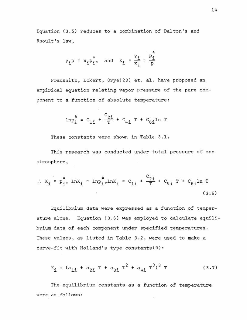
Equation (3.5) reduces to a combination of Dalton's and

Raoult's law,

* y.p = x.p.' ~ ~ ~

and K. -~

* y. p. ~ = ~

x. p ~

14

Prausnitz, Eckert, Orye(23) et. al. have proposed an

empirical equation relating vapor pressure of the pure com-

ponent to a function of absolute temperature:

* lnp. ~

These constants were shown in Table 3.1.

This research was conducted under total pressure of one

atmosphere,

* * . K . = p . , lnK • ~ ~ ~

= lnp. ,lnK. ~ ~

( 3. 6)

Equilibrium data were expressed as a function of temper-

ature alone. Equation (3.6) was employed to calculate equili-

brium data of each component under specified temperatures.

These values, as listed in Table 3.2, were used to make a

curve-fit with Holland's type constants(9):

(3.7)

The equilibrium constants as a function of temperature

were as follows:

Water:

K. 1/3 (T~) = -0.02569219+0.1773240xl0-4T-0.1780874xlO-GT 2

+0.6871899xl0-9T3

Methanol:

K. 1/3 (~) = -0.1228759+0.7404905xl0-4T+0.3787396xl0-6T2

T

Acetone:

(~)l/ 3 =-0.2439641+0.1627855xl0-3T+O.l255913xlO-ST2

-0.8441363xl0-9T3

C. Rigorous Enthalpy Relationships:

15

Like equilibrium data, enthalpy data should be theoreti-

cally a function of both temperature and composition due to

chemical dissimilarity(25).

H. = f 1 (T.,y .. ), for vapor mixture J J ]~

h. = f 2 (T.,x .. ), for liquid mixture J J ]~

or c ...

H. = 1: H. ·Y·. J i=l ]~ ]~

c -h. = 1: h .. x ..

J i=l ]~ ]~

16

D. Assumption for Calculation of Enthalpy Data:

The composition effect is nearly negligible in the

calculation of vapor enthalpies. Thus these may be considered

functions of temperature alone for the calculations made in

this work.

The composition effect is generally not negligible for

the liquid phase, and values of h .. are required. These ]~

would have been easily calculated if experimental partial

molar heats of solution (defined as L .. =h .. -h .. ) over ]~ J~ ]~

the entire range of composition had been available(25).

Since these data were not available, the ideal solution

approximation is made for calculations of vapor and liquid

enthalpies.

c H. = E H .. y ..

J i=l ]~ J~ (3.8)

c h. = 1: h . .'X ••

J i=l J~ J~ (3.9)

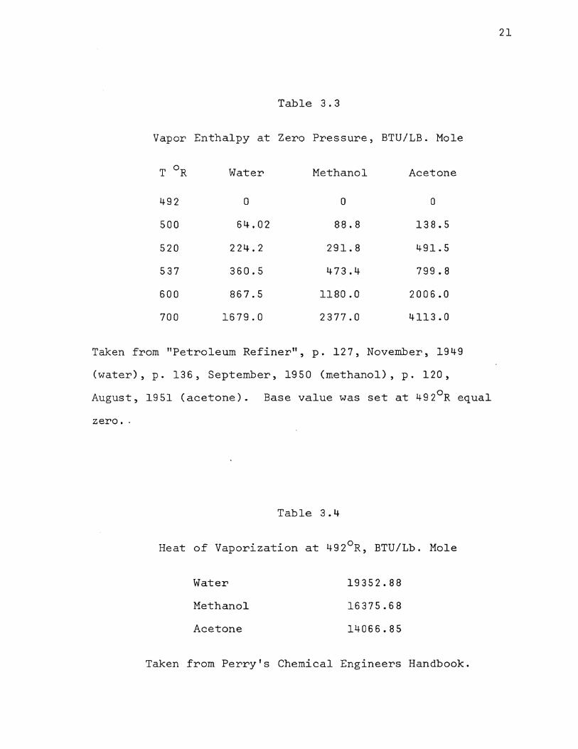
E. Source of Enthalpy Data:

Vapor enthalpy data for these components at zero pres­

sure are available from literature as shown in Table 3-3.

This research, however, was conducted under one atmosphere,

and it is necessary to make a correction for pressure change.

The variation of enthalpy with pressure in a system at

constant temperature is given by

17

(3.10)

By integration at constant temperature,

H = H0 + ]2 (v - T(:~>p) dp (3.11)

1

The Berthelot Equation(l9) is an accurate equati~n of

state and may be differentiated to give the derivative of

volume with respect to temperature at constant pressure.

give

where

( 9 pr

PV = RT 1 + 12 8 T( 1 r

_6 >) T 2

r

(3.12)

This derivative was substituted in Equation (3.11) to

= H 0

T R = Tc'

1.987

Since relative enthalpies with the base value at 492°R

liquid were used, vapor enthalpy should be elevated to a

base value at 492°R liquid equals zero. The heat of vapor­

ization at 492°R (Table 3.4) was added to this base value to

obtain the values shown in Table 3.6.

18

No liquid enthalpy data except for water in the desired

range are available from the literature. However, they could

be calculated by subtraction of latent heat of vaporization

from corresponding vapor enthalpy. The latent heats of

vaporization and liquid enthalpies were shown in Table 3.7,

and Table 3.8 respectively.

The vapor enthalpy equations obtained by least squares

technique were:

Water:

H.~= 0.12375660xl0 3+0.3275642lxlO-lT-0.31256958xlO-ST2 1

Methanol:

H.~= 0.10984052xl0 3+0.31790598xlO-lT+O.l0287539xl0-4T 2 1

Acetone:

H.~ = 0.85837260xl0 2+0.57459815xlO-lT+O.l8562340xl0-4T2 1

The liquid enthalpy equations obtained by least squares

technique were:

Water:

h.~ =-0.5551029lxl0 3+0.l7535334xlOT-0.12486742xl0-2T2 1

Methanol:

h.~ =-0.53609748xl0 3+0.16521577xlOT-O.lll76039xl0-2T2 1

Acetone:

h.~ = -0.6394218lxl0 3+0.19733626xlOT-0.13442990xl0-2T 2 1

19

Table 3.1

Constants for the Vapor Pressure Equation

c In P(atm) = c 1 + f + c4T + C61n T

Constant Water Methanol Acetone

cl 75.7356943 53.3628096 2.0377274

c2 -13252.85658 -10747.48122 -7144.59924

c4 0.0038625784 0.0023612572 -0.0046496708

cs -9.00000 -5.79200 2.00000

Taken from "Computer Calculations for Multicomponent Vapor-

Liquid Equilibria" by Prausnitz et. al. PP218-219, with con­

version of temperature unit from °K to 0 R.

Point No.

1 2 3 4 5 6 7 8 9

10 11 12 13 14 15 16 17 18 19 20 21 22 23 24 25 26 27 28 29 30

Table 3.2

Equilibrium,Data at One Atmosphere

T 0 R Water Methanol

590.399900 0.154216 0.662616 594.000000 0.169627 0.720416 597.599800 0.186333 0.782362 601.199900 0.204422 0.848728 604.800000 0.223983 0.919698 608.399900 0.245109 0.995585 612.000000 0.267917 1.076598 615.599800 0.292486 1.163051 619.199900 0.318942' 1.255180 622.800000 0.347394 1.353265 626.399900 0.377950 1.457635 630.000000 0.410762 1.568570 633.599800 0.445933 1.686378 637.199900 0.483590 1.811457 640.800000 0.523892 1.944002 644.399900 0.566973 2.084433 648.000000 0.612978 2.233099 651.599800 0.662070 2.390325 655.199900 0.714395 2.556474 658.800000 0.770139 2.732045 662.399900 0.829447 2.917225 666.000000 0.892491 3.112580 669.599800 0.959477 3.318384 673.199900 1.030562 3.535098 676.800000 1.106004 3.763206 680.399900 1.185917 4.003102 684.000000 1.270518 4.255173 687.599800 1.360055 4.519873 691.199900 1.454747 4.797816 694.800000 1.554773 5.089201

Acetone

0.956418 1.024495 1.096370 1.172181 1.252083 1.336214 1.424725 1.517770 1.615496 1.718058 1.825610 1.938304 2.056292 2.179739 2.308798 2.443622 2.584370 2.731194 2.884255 3.043698 3.209688 3.382379 3.561916 3.748453 3.942134 4.143122 4.351551 4.567564 4.791301 5.022926

N 0

Table 3. 3

Vapor Enthalpy at Zero Pressure, BTU/LB. Mole

T 0 R Water Methanol Acetone

492 0 0 0

500 64.02 88.8 138.5

520 224-.2 291.8 491.5

537 360.5 473.4- 799.8

600 867.5 1180.0 2006.0

700 1679.0 2377.0 4113.0

Taken from "Petroleum Refiner", p. 127, November, 1949

(water), p. 136, September, 1950 (methanol), p. 120,

August, 1951 (acetone). Base value was set at 492°R equal

zero. -

Table 3.4-

Heat of Vaporization at 492°R, BTU/Lb. Mole

Water

Methanol

Acetone

19352.88

16375.68

14066.85

Taken from Perry's Chemical Engineers Handbook.

21

22

Table 3.5

Critical Properties for Water, Methanol, Acetone

Vapor Water Methanol Acetone

T 0 R c 1165 924 916

PC atm 218.3 78.5 46.6

Taken from Perry's Chemical Engineers Handbook

Table 3.6

Vapor Enthalpy at One Atmosphere, BTU/Lb. Mole

T 0 R Water Methanol Acetone

492 0 0 0

500 66.39 91.31 143.9 4

520 232.08 302.74 509.46

537 372.58 490.16 827.31

600 891.6 5 1214.20 2062.13

700 .1717.07 2429.83 4199.70

Calculated by Computer Program using the Berthelot Equation.

Base value was set at 492°R equal zero.

23

Table 3.7

Latent Heats of Vaporization at One Atmosphere, BTU/Lb. Mole

49 2

500

520

537

600

700

Methanol

1.6375104xl04

1.6280000xl0 4

1.6071000xl04

1.5900000xl04

l.5180000xl0 4

l.3385000xl0 4

Acetone

1.4066856xl04

1.4014000xl04

1.3840000xl04

1.3678000xl0 4

1.2894444xl04

1.1200000x10 4

Taken from J. M. Smith's "Introduction to Chemical Engineer­

ing Thermodynamics", p. 134, Second Edition (1959).

Table 3. 8

Liquid Enthalpy at One Atmosphere, BTU/Lb. Mole

T 0 R Water Methanol Acetone

492 0 0 0

500 145.0 186.99 196. 79

520 505.80 607.42 736.31

537 812.48 965.84 1216.16

600 1949.0 2409.88 3234.540

700 3753.0 5420.51 7066.55

Obtained by subtraction of latent heat of vaporization from

vapor enthalpy. Base value was set at 492°R equal zero.

IV. CALCULATIONAL PROCEDURE TO DETERMINE PLATE EFFICIENCY FROM EXPERIMENTAL DATA

24

Determination of experimental efficiency was based upon

the operating data of an existing distillation unit, the

liquid-vapor equilibrium relationship of mixture, and the

material and the energy balance around each plate. Plate­

to-plate calculation could proceed either from the top down

to the reboiler or vice versa.

A. Degrees of Freedom in Multicomponent Distillation

Column(7):

The independent variables describing the operation of a

multicomponent distillation unit are of two types: the

thermodynamic intensive.variables and the relative quantities

of the- various streams of matter and energy. The "Phase

Rule" enunciates the .degrees of freedom of a system as the

number of independent intensive thermodynamic properties

present. It states

F = C - P + 2

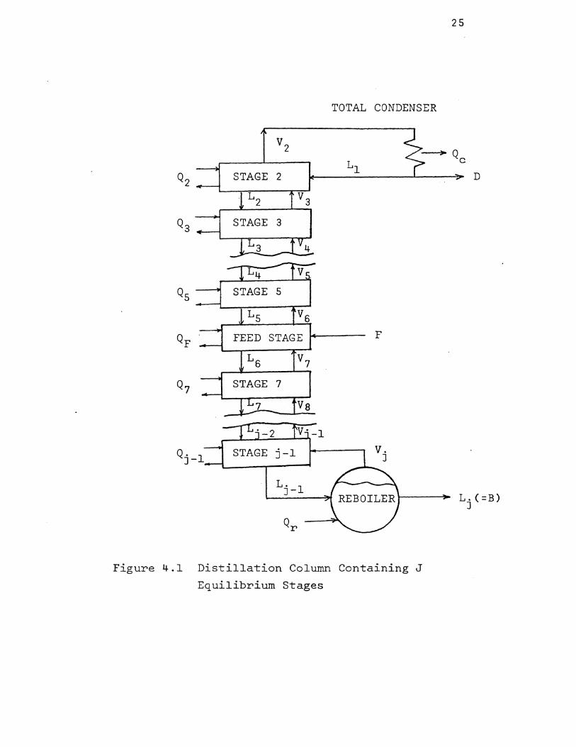
A distillation unit may be considered as j contacting

stages in series (Figure 4.1); each stage functions as a

mixer and adiabatic separator (Figure 4.2). The inlet

stream(s) enters the mixer while two equilibrium outlet

streams leave the separator. A detailed analysis of the

whole distillation unit is divided into four parts:

Q . F

2

j-1

L. 1 ]-

TOTAL CONDENSER

F

Figure 4.1 Distillation Column Containing J

Equilibrium Stages

25

D

L. (=B) J

L. 1 ]-v.

J

ADIABATIC

SEPARATOR

Q. J

Figure 4.2 Operational Representation of a

Single Contacting Stage j

26

L. J

27

Al. Condenser

There is one inlet stream and two outlet streams around

the total condenser (Figure 4.5). The feed to the condenser

is a one-phase system possessing (C + 1) degrees of freedom.

Since the reflux and distillate are each one-phase systems

of identical composition and condition, they account together

for a total of (C + l) degrees of.freedom. There are two

quantity ratios and one heat ratio (with one quantity ratio

fixed at unity) corresponding to the three streams. There­

fore the total number of variables associated with the conden­

ser is 2C + 5. There are C compon.ent material balances and

one enthalpy balance; thus the number of independent varia­

bles is C + '+.

A2. Single Stage (Excluding Feed Stage)

It is assumed that the two streams leaving any plate

are in equilibrium and therefore constitute a two-phase,

thermodynamic equilibrium system (Figure 4.3). This two­

phase system and the two one-phase streams entering each

plate possess a total of (3 C + 2) degrees of freedom.

Associated with each plate are four quantity ratio variables

and one heat ratio variable. The total number of independent

intensive variables, quantity ratios, and heat ratio then

becomes:

(3 C + 2) independent thermodynamic intensive variables + 4

quantity ratios + 1 heat ratio.

28

'

fli~·J Li·• ~hF }--1

Q i ~;1 Li 'i·.f~fli .

l t-/

Fig~re 4.3 Operational Representation of Si~gle Stage j in a

Distillation Column with TJ., and x .. Fixed by Jl.

Experiment

•

1#-i 4-· \j,,f r~'

.1= Xf4 • r ~

~t? '-f.· ft# ' }""'

Figure 4.4 Operational Representation of Feed Stage in a

Distillation Column with Tj, xji F, and xFi Fixed by Experiment

Relating these variables are a total of C independent

material balances and one independent enthalpy balance.

Besides, one quantity ratio is fixed at unity. Therefore

the total number of degrees of freedom is 2 C + 5.

A3. Feed Stage

29

Since there are three one-phase streams entering the

feed stage, and one two-phase stream leaving in equilibrium

(Figure 4.4), with one quantity ratio fixed at unity, the

number of independent intensive variables and quantity ratios

associated with this plate is:

3(C + 1) independent intensive variables in feed streams + C

independent intensive variables in equilibrium exit streams

+ 5 quantity ratios + 1 heat ratio -1 quantity ratio fixed

at un~ty.

There are C independent material balances and one enthalpy

balance, therefore the total number of independent variables

is 3 C + 7.

A4. Reboiler

A single one-phase stream is entering the reboiler, and

two streams in equilibrium with each other are leaving the

reboiler (Figure 4.6). By the "Phase Rule", these streams

together possess (2 C + 1) independent intensive variables.

Also associated with the reboiler are three quantity ratios

and one heat ratio, making a total of 2 C + 5.

~) ~~ r------------------,

~-----12

t----~3 Qc

L, ~~ )

30

Figure 4.5 Opera~ional Representation of Total Condenser in

a Distillation Column with TD' xDi' D, 11 , and

x1 i Fixed by Exper~ment

' Ltr

B

Gr Figure 4.6 Ope:rationai Representation of Partial Reboiler in

a Distillation Column with B, TB, XBi and Q r Fixed by Experiment

Relating these variables are C independent material

balances and one independent enthalpy balance. Therefore

the total number of independent variables is C + 1.

B. Vapor Composition and Internal Flow Rates

31

For an experimental run on the distillation tower (des­

cribed in Appendix C)the reboiler duty, the reflux rate, and

the bottoms product rate are controllable and are maintained

at specified values. The feed composition is determined by

the make-up of the particular mixture chosen for a run and

placed in the feed tank. The feed temperature is specified

and is controlled by adjusting a feed preheater. During the

run the tray temperatures may be recorded from the column

instruments (with the exception of the second stage or top

tray) and samples may be withdrawn from each internal over­

flow stream. The composition of the internal overflow

streams is determined from the analysis of these samples.

For a complete column description each variable which

may be specified or determined from operational data reduces

the required number of equations by one. The remaining

equations for this column may be developed from heat and/or

material balances written around the condenser, the reboiler,

and around each tray of the column. Modifications of the

general tray balances are required for the feed tray and for

the first tray. The special approach to the first tray is

necessary to determine its operating temperature which is

not available from recorded data.

32

Bl. Total Condenser

As analyzed in Section Al, the number of independent

variables for the total condenser is C + 4. The experimental

data specify ( C - 1) compositions, the distillate rate, the

reflux rate, the stage temperature, and the stage pressure.

Therefore only one equation is left to determine the conden­

ser duty. It is readily solved, because an enthalpy balance

around the whole distillation tower states:

(B.l)

This condenser duty is calculated by the programs

referred to in block 3 of Figure 4.7, the flow chart for the

computer program.

~2. Calculation of Second Stage Temper~ture

Because there is no thermocouple on the second stage of

the experimental column used, a special calculation must be

made to determine its operating temperature before an effi­

ciency calculation is made·. There are ( C + I+) independent

variables around the total condenser. The experimental data

specify (C + 3) variables, such as (C- 1) compositions, the

distillate rate, the reflux rate, the stage temperature, and

the stage pressure. An enthalpy balance equation around the

total condenser can be used to solve for the enthalpy of the

vapor stream leaving the second stage. It states

33

H2 Llhl + D hD + Qc

= Ll + D

or

H2 (R•D)h1 + D hD + Qc

(B2.1) = {R•D) + D

These enthalpies, calculated from tower composition

data, are determined by the programs shown in block 4 of

Figure ~.7, the flow chart for the computer program.

The enthalpies of the reflux and of the distillate are

equal to each other. The reflux was neither heated nor

cooled before it entered the second stage. If the enthalpy

is a function of temperature alone, a fourth order algebraic

equation must be solved to determine the stage temperature.

This equation could be solved by using either the Newton or

the False Position Method(9) to obtain accurate temperature.

This equation states

c E H2.y2.' . 1 ~ ~

~=

~ where H2i =

= A + B T2 + C T 2 + D T 3 + F T q 2 2 2 (B2.2)

The vapor composition of ~he second stage is the same as

that of the first stage, and is also identical with the

34

liquid composition on the first stage. The total condenser

causes only a phase change in the stream. A, B, C, D, and

Fare all calculated constants, which stand for the product

of enthalpy coefficients and vapor composition of the second

stage. These are all known values as shown in Equation

(B2.2).

The iterative procedure required to determine the tern-

perature of the second stage is referred to in block 5 of

Figure 4.7. It includes the following steps:

1. The estimated second stage temperature is first

calculated from experimental first and third stage

temperature.

2. The second stage temperature estimated in Step 1 is

used to calculate the estimated enthalpy.

~. The estimated enthalpy value is compared with the

correct enthalpy

}<H2)estima~ed -

value calculated in Step (b). If

(H ) I < E the second stage 2 correct '

temperature has been determined.

4. If the test condition is not met, return to Step 2,

using the revised value for the stage temperature.

B3. Single Stage Equations

As analyzed in Section A2, the total number of indepen-

dent variables for each stage is 2 C + 5. The experimental

data determine (C- 1) liquid compositions, x. 1 ., the J- ,l

stage temperature, T. 1 , and the· stage pressure, P. 1 . The J- J-

35

liquid overflow from the tray above, L. 1', is determined )-

prior to solving the balances for tray j. Similarly, for

the liquid stream leaving the stage j, the experimental data

determine (C- 1) liquid compositions, x .. , the stage tem-J1

perature, T., and the stage pressure, p .. Therefore C J J

variables remain to be solved by two equations around stage

j. There are C component material balances around stage j

and one enthalpy balance around stage j.

The component material balance equation is used to solve

for the composition of the entering vapor stream, y.+l .. J ,1

The enthalpy balance equation is used to solve for the flow

rate of leaving liquid stream, L .• These equations are J

stated as follows:

(1) A component material balance equation around stage j

s~ates

L.x .. - L. 1x. l . + (L. l + D- F)y .. = J ]1 J- ]- ,1 ]- ]1 L. + D - F

J (B3.1)

(2) An enthalpy balance equation around stage j states

(B3.2)

(3) An overall material balance equation around the section

which encompasses the stage j and the total condenser

states

V. = L. l + D - F J )-(B3.3)

36

For the rectifying section, F should be zero in Equation

(B3.3). By stage-to-stage calculation from the top of the

distillation tower down to the reboiler, Equation (B3.1)

determines the vapor composition of the entering stream,

y.+l . , while Equation (B3.2) is used to calculate the flow J ,~

rate of leaving liquid stream, L .• These C + 1 independent J

equations may be solved simultaneously to determine the values

of the C + 1 unknown variables. The nature of these equa-

tions is such that an iterative procedure must be used to

solve them.

An iterative procedure for each stage is required to

determine y.+l ., and L .. ] ,1 J

1. Beginning with stage 2, L. is assumed to be equal to J

2 •

3 •

L. 1 , which may be obtained from experimental data. ]-

This step is taken in block 6 of Figure 4.7.

In block 10 it is shown that the initial value for

each yj+l,i' is set at the value determined for yji'

Equation (B3.1) is solved for y.+l . as shown in J ,1

block llA of Figure 4.7.

4. Equation (B3.2) is solved for L., using the values J

of yj+l,i calculated in Step 3. This enthalpy balance

is included in blocks 13A and l3B of Figure 4.7 •.

5. Equation (B3.3) is solved for V., using the value of J

L. 1 , calculated in Step 4. This overall material ]-

balance is shown in blocks 9A and 9B of Figure 4.7.

37

6 . The values of the y.+l . are compared with the pre­] ,~

vious (or estimated) values. This action is shown

in blocks 14A and 14B of Figure

If I (y. . ) · d - (y. 1 . ) . d I < e:, the solu-J+l,~ rev~se J+ ,~ est~mate

tions for this stage have been determined. The calculations

for the next stage should be initiated as shown in blocks 15

and 16 of Figure 4.7. If the test conditions are not met,

control is returned to Step 2, (block llA), and new trial

values are calculated for Lj and the Yj+l,i's.

B4. The Feed Stage

The feed stage has (3 C + 7) independent variables as

analyzed in Section A3. The experimental data specify

(C + 2) variables for the entering liquid stream, and the

feed s_tream respectively. The leaving liquid stream is

specified by (C + 1) known variables such as (C - 1) liquid

compositions, the stage temperature, and the stage pressure.

Therefore two unknown variables are left to be solved for by

two equations around this stage. The component material

balance equation is used to solve the composition of entering

vapor stream, yj+l,i. The enthalpy balance equation is used

to solve for the flow rate of leaving liquid stream, L .• J

These equations are mathematically expressed as follows:

(1) A component material balance equation around feed stage

states

L. x. . - L. ·1 x . l . + ( L. l + D - F) y . . - FXF1• = J J~ ]- ]- ,J. ]- ]J. L. + D - F

J

38

(B4.1)

(2) An enthalpy balance equation around feed stage states

L. 1 <H. - h. 1 > L = ]- J ]-.

+ D(H. - H.+l) J J

J Hj+l - hj

(B4.2)

(3) An overall material balance equation around the section

which emcompasses the feed stage and the total condenser

states

V. = L. l + D ) ]-

(B4.3)

As explained in Section B3, the Equation (B4.l) expres­

ses yj+l,i as a function of Lj, and the Equation (B4.2)

expresses L. as a function o.f y.+l . . An iterative procedure J J ,J.

is required to solve for these three unknown variables.

The iterative procedure for the feed stage is outlined

J.n the following steps:

1. L. is equal to the sum of the feed rate and the . )

liquid rate leaving the stage immediately above the

feed. The latter value is available from earlier

calc~lations in the rectifying section.

2. Equation (B4.1) is solved for y.+l .. J ,~

3. Equation (B4.2) is solved for L., using the values J

of y.+l . calculated in Step 2. J ,~ .

4. Equation (B4.3) is solved for V., using the value of J

L. 1 calculated in Step 3. J-

39

5 • The values of the y.+l . . J ,~ are

vious (or estimated)

- (yj+l,i)estimatedl

values.

compared with the pre­

If l(y.+l .) . J ,~ rev~sed

< e, this stage is solved.

If the test conditions are not met, return to Step 2,

using the revised value for the L .. J

BS. The Reboiler

The reboiler possesses (C + 1) independent variables as

analyzed in Section A4. The experimental data specify (C - 1)

bottoms compositions, xBi' the bottoms rate, and the bottoms

temperature. Therefore the reboiler is fixed by experimental

data. Solution of the heat and material balances written

around the reboiler would therefore yield no new information.

C. Efficiency Calculations

As described in Section B3 and B4, the vapor composi­

tions and stream flow rates can be calculated from experimen-

tal data by iterative procedures. Once all of the vapor

compositions have been determined the plate efficiency may

be calculated. They are mathematically expressed as follows:

Modified Murphree Plate Efficiency(9)

M E .• )~

= Yji - Yj+l,i y. . - y. +1 . ]~ J ,~

(C.l)

40

Vapc :•ization E£ficiency(9)

v E .• Jl

= yji y •. (c. 2)

]1

Where Y .. is ideal vapor compositions which would be in ]1

1uilibrium with liquid, and is mathematically expressed as

)llows :·

Y .• = K •• * x .. (9) ]1 ]1 Jl

D. Model Validation

The calculational model developed in Section B is tested

.th hydrocarbon and non-hydrocarbon systems on a hypotheti­

Ll simulated distillation tower with component efficiencies

:t equal to unity. For a third trial system, the efficien-

.es for the non-hydrocarbon case were given random values .

. e hypothetical distillation towers have the same number of

grees of freedom as the experimental tower, and the oper-

ing conditions are arbitrarily specified. The calculated

.por compositions and the stream flow rates are both within

e desired accuracy when compared to the known data taken

om the hypothetical tower. Three test problems are shown

Table 4.1,-Table 4.2, and Table 4.3. The calculated

sults are compared to the standard values in Table 4.4,

ble 4.5, and Table 4.6.

The method used to simulate. the above columns was the

-method of convergence for a conventional column" proposed

41

by Holland(9). The input known variables include feed rate,

distillate rate, bottoms rate, external reflux ratio, feed

compositions, feed temperature, assumed vaporization effi­

ciencies, assumed temperature profile, assumed vapor and

liquid stream flow rates. The outputs from the simulation

program are correct temperature profile, vapor and liquid

stream flow rates, vapor and liquid compositions, condenser

duty, and reboiler duty when e converge to unity.

The simulation program as well as the program used for

efficiency calculations is given in Appendix E.

E. Application to Experimental Data

This method of calculating distillation efficiencies

was also applied to experimental data obtained on a labora­

tory ~istillation column. The column characteristics and

operating procedures used are given in Appendix C. Since

there is no way of experimentally checking the efficiencies

at various points in the column without measurement of vapor

compositions, which was not feasible in the runs made, the

application to experimental data does not verify the methods

developed. However, it does provide an example of the poten­

tial use of the methods. This example can be partially

verified by the use of the obtained efficiencies in a dis­

tillation simulation program, to see if calculated perfor­

mance matches the experimental data used to determine effi­

ciencies. The results of the efficiency calculations from

experimental data are given in Tables 4.7 to 4.10. The

simulation results using calculated efficiencies are in

Table 4.11.

42

F~gure 4.7

Flow Chart for the Efficiency Calculation

Read in Operating Dat"a, Enthalpy Coefficients, and Equilibrium Constants

Calculate External Streams Enthalpies hF = EhFixFi

2.

Calculate Condenser Duty 3 •

QC = FhF+QR-Bh8-DhD (B.l)

Calculate Enthalpy of Vapor Stream 4. Leaving Second Stage

H2 = (L1h1+DhD+QcfV 2 (B2.1)

1

5 .;:­

.w

a

Set F = 0

v •.

H2 = H2iy2i = f(T2)

. 2 3 4 = A+BT 2+CT 2 +DT 2 +FT 2 (B2.2)

6 , Ass( urn) e L ( 1 ) L 2 =

7. Initiate NI = 1 NTT = 2

NI: Number of Iteration· NTT: Number of Stage j Feed Stage is at 6th.

~~,~---------------<---------~=?Calculate Vapor Stream Flow Rate gB v. = L. l + D • J J-

> ~------~~~----------~

. Calculate Vapor Stream Flow Rate '----~

Calculate Liquid Stream Flow Rate "'9A.

V. = L. 1+D-F (B3.3) J J-

Assume lOA.

'

Yj+l)iiNI = Y•. J~

Ljll = Lj-liNN+F

1

Assume

Y• 1 . I J+ ,~ 1 = Y ..

1 1oB.

J~ NN

-~

a

llA~Calculate Vapor Stream Compositions

y. + 1 i I = fL. x .. -L. lx. 1 . J ' NI+l t J Jl. .J- J- ' 1

+(L. 1 +D-F)y . . )ltr .+D-F) (B3.1) ]- ·J~ ".UJ

Calculate Stream Enthalpies 12A.

Hj, Hj+l' hj' hj-l

Calculate Liquid Stream Flow .----__...;~ 13A. Rate

L., =(L. 1CH.-h. ·1)+D(H.-H.+l) J NI + 1 J - J J - J J

+F(Hj+l-Hj~/Q:ij+l-hj) (B3.2)

b c

llB.Calculate Vapor Stream Com­positions

Y·+l ·I =[L.x .. -L. lx. 1 . J ' 1 NI+l J Jl. J- J- ' 1

+(L. 1+D-F)y .. -FXFJ/~.+D-F) J- Jl. ~ J

(B4.1)

Calculate Stream·Enthalpies 12B. .

H., H. +l, h. , h. l J J J J-

Calculate Liquid Stream Flow Rate - Leaving Feed Stage

13B. [ . Lj INI+l = Lj-l(Hj-hj-1)

+D(Hj-Hj+l)+F(Hj+l-Hj-hF~/

(Hj+l-hj) (B4.2)

+ <.n

a

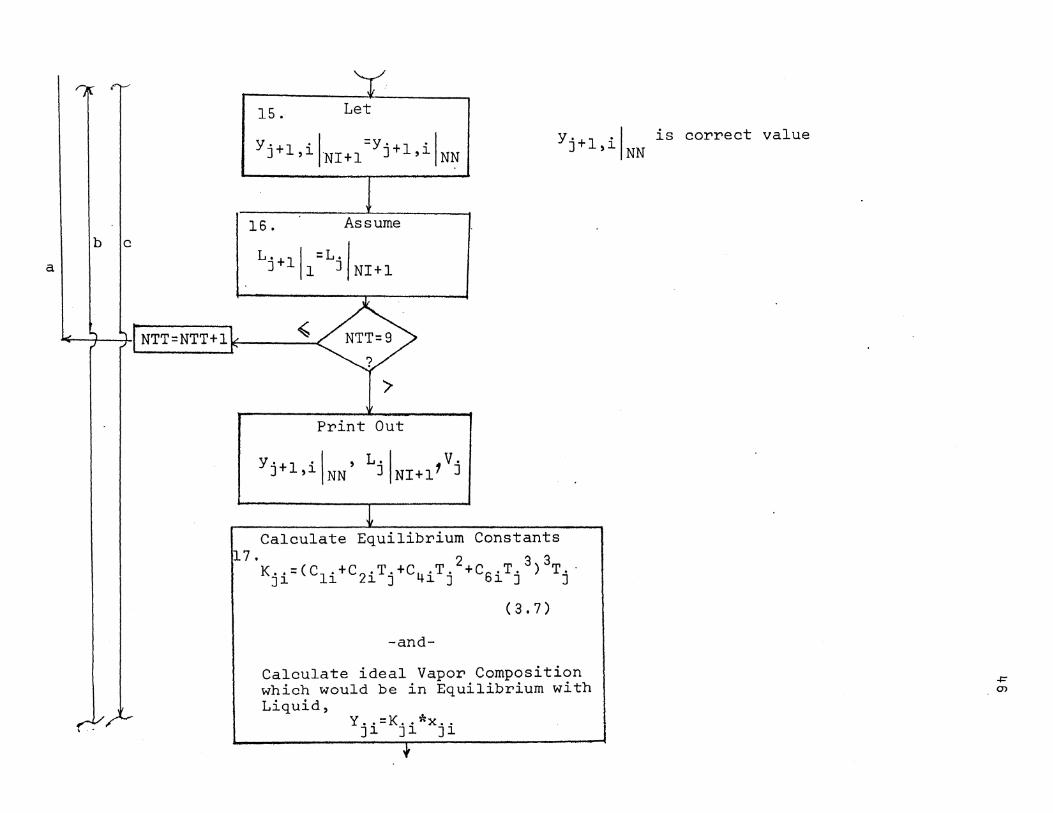
y 15. Let

y. 1 ., =y. 1 ., J+ ' 1 NI+1 J+ ' 1 N~

16. Assume b c

Lj+lll=LjiNI+l

yJ'+l I is correct value ,i NN

"' ~-~ NTT=NTT+lr~r----~---<.:<2;> >

Print Out

y.+l'l ,L., V. J ' 1 NN J NI+11 J

Calculate Equilibrium Constants tJ.7. 2 3 3

K .. =CC1 .+c 2.T.+C4 .T. +C6 .T. ) T. · ]1 1 1 J 1 J 1 J J

( 3. 7)

-and-

Calculate ideal Vapor Composition which would be in Equilibrium with Liquid,

Y •• =K .• *x .. ]1 ]1 ]1

b c

18. Calculate Vaporization Efficiency (VE)

E •• 0 = y .. IY .. J~ J~ J~

(c. 2)

-and-

Murphree Plate Efficiency (PE)

El;f · = (y' '-y' +1 .)/(Y" -y '+1 ' ) ( C .1) J~ J~ J ,J! J~ J ,~

Function Subprogram Calculate Stream Entha1pies

HJ. = l: H • • y • • , h • = l: h • • x . . etc • J~ J~ J ]1 ]1

Table 4.1

Statement of Numerical Test for Calculational Procedure on Hydrocarbon System with Efficiency Equals to Unity

Spec1.f1.cat1.ons Data for D1.st1.llat1.on Plate Eff1.c1.enc1.es Calculat1.ons

Component Feed Liquid Comp. Mole Frac. Component Feed Rate Comp. Stage T 0 R N-C 3 N-C N-C5 Lb.Mole/Hr. Mole Number 4

Frac.

Propane 33 0.33 l.(Condenser) 625.3027 0.6418696 0.3517753 0.0063547

N-Butane 33 0.33 2 . 648.7966* 0.4191279 0.5567314 0.0241408

N-Pentane 34 0.34 3 . 665.8925 0.2875983 0.6564091 0.0559927

Feed Rate 100 Lb.Mole/Hr. 4. = 677.3037 0.2211437 0.6727295 0.1061264

Distillate Rate 50 Lb.Mole/ 5 • 6 86.20 82 0.1880474 0.6348891 0.1770635 =

Hr. 6 • 694.6486 0.1698862 0.5650709 0.2650431

Bottoms Rate = 50 Lb.Mole/Hr. 7. (Feed) 703.0651 0.1581966 0.4831434 0.3586599

Reflux Rate = 100 Lb.Mole/Hr. 8. 721.0854 0.0872821 0.4741603 0.4385577

Boiling Point Liquid Feed, 9 • 738.7072 0.0427546 0.4104019 0.5468435 Total Condenser, Ten Stages 10.(Reboiler) 756.0747 0.0181301 0.3082241 0.6736456

Including the Reboi1er, Distillation Column Pressure Miscellaneous Data:

= 300 psia The Equilibrium Data and Condenser Duty = 1039340 BTU/Lb.Mole

Enthalpy Feed Temperature = 676.4080°R Data are Given in Table A-4

and Table A-8 of Ref. * ( 9 ) Calculated

Spec1f1cat1ons Data for D1st1llat1on Plate Efficiencies Calculations

Component Feed Liquid Comp. Mole Frac.

Component Feed Rate Comp. Stage T 0 R Water Methanol Acetone Lb.Mole/Hr. Mole Number Frac.

Water 1.91983 0.5625 l.CCondenser) 599.65280 0.0104540 0.8189646 0.1705809 Methanol 1.27193 0.3725 2 . 601.91650* 0.0424265 0.8285156 0.1290581 Acetone 0.22301 0.0650 3 . 603.76870 0.1098638 0.7847897 0.1053467

4. 608.20230 0.2275898 0.6847721 0.0876387

Feed Rate 3.41 Lb.Mole/Hr. 5. 614.63350 0.3805187 0.5477149 0.0717667 = 6. (Feed) 621.45190 0.5200827 0.4210669 0.0588508 Distillate Rate = 1,12 Lb. 7. 622.97260 0.5463138 0.4040496 0.0496366

Mole/Hr. 8 . 626.26070 0.6028088 0.3585168 0.0386741

Bottoms Rate = 2.29 Lb.Mole/ 9 • 632.60740 0.7032492 0.2708313 0.0259201

10. C Rebo~ler) 642.15470 0.8324966 0.1541414 0.0133622 Hr.

Reflux Rate = 1.570 Lb.Mole/ Enthalpy Equations: xl0- 2T2 Hr.

h~ = -0.5551029lxl0 3+0.l7535334xlOT-0.12486742 -5 Boiling Point Liquid Feed Water H~ O.l2375660xl0 3+0.3275642lxl0-lT-0.31256958xl0 2 = Total Condenser, Eight Trays T

Reboiler, Distillation Methanol

h~ = -0.53609748xl0 3+0.l6521566xlOT-O.lll76039xl0-2T2 Column Pressut"e Maintained at

H~ = O.l0984052xl0 3+0.31790598xl0-1T+O.l0287539xl0-4T2 One Atmosphere.

Acetone

h~ = -0.6394218lxl0 3+0.l9733626xlOT-0.13442990xl0-2T2

H~ = 0.85837260xl0 2+0.57459815x10-lT+0.18562340xl0- 4T2

Miscellaneous Data: Condenser Duty = 38855.80-BTU/Lb.Mole -- Feed Temp. = 623.58400R *Calculated

Table 4.3

Statement of Numerical Test for Calculational Procedure on Non-Hydrocarbon System with Made-up Random Efficiency

Spec~f~cat~ons Data for D1st1llat1on Plate Eff1c1enc1es Calculat1ons

Component Feed Liquid Comp_os it ions Mole Frac.

Feed Rate Comp. Stage T 0 R Component Lb.Mole/Hr. Mole Number Water Methanol Acetone Frac.

Water 1.9198 0.5625 l.(Condenser) 599.0292 0.0002508 0.8067961 0.1929532

Methanol 1.2719 0.3725 2. 615. 7465* 0.0021573 0.8867980 0.1110455

Acetone 0.2230 0.0650 3 . 601.3769 0.0153424 0.8944494 0.0902090

Feed Rate ;; 3.41 Lb.Mole/Hr. 4 . 623.8000 0.401418 0.9171325 0.0427262

Distillate Rate = 1.12 Lb. 5. 605.0327 0.1389493 0.8169599 0.0440916

Mole/Hr. 6. (Feed) 621.8903 0.4470339 0.5226896 0.0302764

Bottoms Rate ;; 2.29 Lb.Mole/ 7 • 625.9306 0.4785022 0.5086399 0.0128580 Hr.

8. 631.5791 0.5541156 0.4361750 0.0097092 Reflux Rate ;; 1.57 Lb.Mole/Hr. 9. 647.0654 0.7092515 0.2859765 0.0047718

10. (Reboiler) 642.7292 0.8374869 0.1600931 0.0024204 Boiling Point Liquid Feed,

Total Condenser, Eight *Calculated

Trays, Reboiler, Distilla-

tion Column Pressure Main-

tained at One Atmosphere

c.n 0

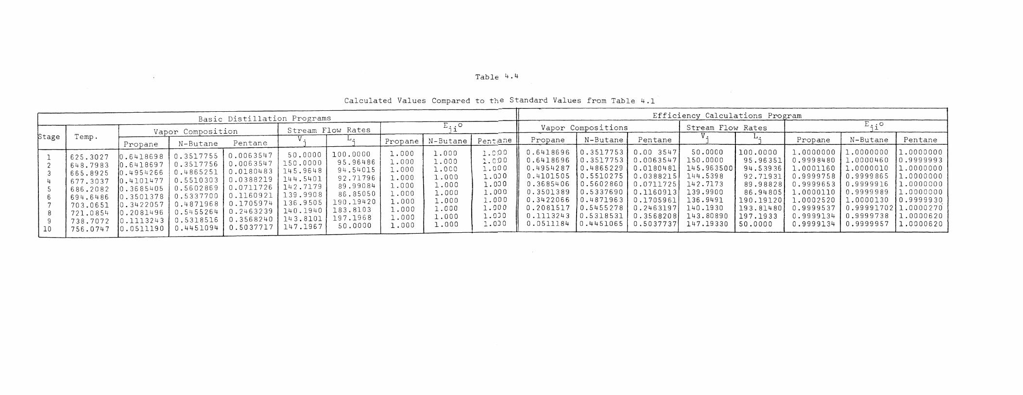
Table 4.4

Calculated Values Compared to the Standard Values from Table 4.1

Basic Distillation Programs Efficiency Calculations Pro ram

Vapor Composition Stream Flow Rates E .. o Vapor Compositions Stream Flow Rates

E .. o

!Stage Jl

. -; l

Temp. v-i Lj N-Butane Propane N-Butane Pentane v. Ll Propane N-Butane Pentane Propane PentiCine J Propane N-Butane Pentane

1 625.3027 0.6418698 0.3517755 0.0063547 50.0000 100.0000 1.000 1.000 1.0:00 0.6418696 0.3517753 0.00 3547 50.0000 100.0000 1.0000000 1.0000000 1.0000000

2 648.7983 0.6418697 0.3517756 0.0063547 150.0000 95.96486 1.000 1.000 l. o:oo 0.6418696 0.3517753 0.0063547 150.0000 95.96351 0.9998480 1.0000460 0.9999993

3 665.8925 0.4954266 0.4865251 0.0180483 145.9648 94.54015 1.000 l.OCO 1. 0 0 0 0.4954287 0.4865229 0.0180481 145.963500 94.53936 1.0001160 1.0000010 1.0000000

4 677.3037 0.4101477 0.5510303 0.0388219 144.5401 92.71796 1.000 1.000 1. OJ 0 0.4101505 0.5510275 0.0388215 144.5398 92.71931 0.9999758 0.9999865 1.0000000

5 686.2082 0.3685405 0.5602869 0.0711726 142.7179 89.99084 1.000 1.000 1. 00 0 0.3685406 0.5602860 0.0711725 142.7173 89.98828 0.9999653 0.9999916 1.0000000

6 694.6486 0.3501378 0.5337700 0.1160921 139.9908 86.85050 1.000 l. 000 l. ooo 0.3501389 0.5337690 0.1160913 139.9900 86.94805 1.0000110 0.9999989 1.0000000

7 703.0651 0.3422057 0.4871968 0.1705974 136.9505 190.19420 1.000 1.000 l. 00 0 0.3422066 0.4871963 0.1705961 136.9491 190.19120 1.0002520 1.0000130 0.9999930

8 721.0854 0.2081496 0.5455264 0.2463239 140.1940 183.8103 1.000 l. 0 00 l. 00 0 0.2081517 0.5455278 0.2463197 140.1930 193.81480 0.9999537 0.99991702 1.0000276

9 738.7072 0.1113243 0.5318516 0.3568240 143.8101 197.1968 1.000 1.000 l. 0) 0 0.1113243 0.5318531 0.3568208 143.80890 197.1933 0.9999134 0.9999738 1.0000620

10 756.0747 0.0511190 0.4451094 0.5037717 147.1967 50.0000 1.000 1.000 l. OJ 0 0.0511184 0.4451065 0.5037737 147.19330 50.0000 0.9999134 0.9999957 1.0000620

Table 4.5

Calculated Values Compared to the Standard Values from Table 4.2 I

Basic Distillation Programs I Efficiency Calculations Programs Ejio I

Vapor Compositions Stream Flow Rates I Vapor Co~ositions Stream Flow Rates Ejio I Stage Temp. Acetone vj Lj Water Methanol Ace"tor,el Water Methanol Acetone v. L.

Water Water Methanol

J J Methanol Acetone l 599.6528 0.0104540 0.8189655 0.1705808 1.12000 1.56800 l. 000 1.000 1.000 0.0104540 0.8189646 0.1705809 1.119999 1.567998 1.00000 1.00000 1.00000 2 601.2329 0.0104540 0.8189653 0.1705809 2.68800 1.54645 l. 000 l. 00 0 1.000 0.0104540 0.8189646 0.1705809 2.6879980 1.5505620 0.9696383 0.9862729 0.9824863 3 603.7687 0.0289969 0.8245041 0.1464992 2.66645 1.51694 l. 000 1.000 1.000 ::J.0290176 0.8245099 0.1464722 2.6705620 1.5185660 0.9999918 0.9997904 0.9997186 4 608.2023 0.0676403 0.7993056 0.1330544 2.63694 1.47540 l. 000 l. 000 l. 0 00 ).0676670 0.7992957 0.1330367 2.6385660 1.4769850 0.9999804 0.9998898 0.9998467 5 614.6335 0.1338882 0.7426812 0.1234310 2.59540 1.42965 l. 000 1.000 l. 0 0 0

I J.1339458 0.7426450 0.1234090 2.5969850 1.4312020 0.9999147 0.9998083 0.9997249 6 621.4519 0.2179581 0.6668689 0.1151734 2.54965 4.82549 l. 00 0 1.000 l. 00 0 J.2180570 0.6667953 0.1151468 2.5512030 4.8309860 0.9997369 0.9997764 0.9996689 7 622.9726 0.2379199 0.6621458 0.0999346 2.53549 4.79868 1.000 1.000 l. 000 ).2378564 0.6609544 0.0993092 2.5409820 4.8041310 0.9957421 0.9937279 0.9899784 8 626.2607 0.2850776 0.6321739 0.0827488 2.50868 4.74909 l. 000 1.000 1.000 ).2849659 0.6309986 0.0821343 2.5141420 4.7545360 0.9952991 0.9925786 0.9864598 9 632.6074 0.3889150 0.5488397 0.0622456 2.45909 4.672051 1.000 l. 00 0 l. 0 00 ).3886942 0.5477256 0.0616398 2.4645260 4.6774120 0.9933385 0.9902653 0.9756176 10 642.1547 0.5789950 0.3830125 0.0379926 2.38205 2.29000 1.000 1.000 1.000 ).5785592 0.3820444 0.0373941 2.3874130 2.2899990 0.9933385 0.98425 4 0.9756176

Table 4.6

Calculated Values Compared to the Standard Values from Table 4.3

Basic Distillation Programs Efficiency Calculations Pro_grams

~tage Temp. Vapor Compositions Stream Flow Rates Ejio Vapor Com~ositions Stream Flow Rates E-jio vj L-j i v"i Lj Water Methanol Acetone Water Methanol Acetone 'i'Ja ter Methanol Acetone Water Methanol Acetone

l 599.0292 0.0002508 0.8067966 0.1929530 1.12000 1.56800 l. 00 0 1.000 l. 000 CJ.0002508 0.8067961 0.1929532 1.119999 1.5679980 1.0000 1.0000 1.0000 2 615.7465 0.0002508 0.8067967 0.1929531 2.68800 1.64582 0.321 0.654 0. 9 89 I 0J.0002508 0.8067961 0.1929532 2.6879980 1.6458220 0.3210242 0.6540031 0.9889998 3 601.3769 0.0013853 0.8544015 0.1442136 2.76582 1.52863 0.365 0.963 l. 2 06 0.0013853 0.8544018 0.1442134 2.7658220 1.5286230 0.3649967 0.9629986 1.2059880 4 623.8000 0.0089607 0. 8573837 0.1336559 2.64863 1.63155 0.502 0.560 l. 5 30 0.0089608 0.8573840 0.1336555 2.6486230 1.6315450 0.5020087 0.5599968 1.5300120 5 605.0327 0.023904l+ 0.8722202 0.1038758 2.75155 1.49582 0.630 0. 9 86 l. 6 52 0.0239043 0.8722205 0.1038751 2.7515460 1.4958200 0.6299961 0.9859940 1.6519960 6 621.8903 0.0795632 0.8126075 0.1078293 2.61582 4.90278 0.420 0.972 1.805 0.0795634 0.8126079 0.1079286 2.6158200 4.9027860 0.4200025 0.9719953 1.8049830 7 625.9306 0.1048133 0.8404958 0.0546914 2.61278 4.87981 0.467 0.944 2.000 0.1048178 0.8404901 0.0546910 2.6127880 4.8798110 0.4670250 0.9440005 2.0000500 8 631.5791 0.1610734 0.8168392 0.0220874 2.58981 4.81588 0.539 0.945 0.965 0.1610752 0.8169366 0.0220872 2.5898070 4.8l58840 0.5390093 0.9450021 0.9650069 9 647.0654 0.2972075 0.6864756 0.0163174 2.52588 4.76127 0.537 0.872 1.105 0.2972086 0.6864722 0.0163162 2.5258840 4.7612750 0.5370036 0.8719929 1.1049990 10 642.7292 0.590422 0.4026274 0.0069508 2.47127 2.29000 1.000 1.000 1.000 0.5904236 0.4026235 0.0069506 2.4712750 2.2899990 1.0000 1.0000 1.0000

Table 4.7

Column Operating Specifications for the Experimental Run

Component Feed Composition

Water 0.5625

Methanol 0.3725

Acetone 0.0650

Reboiler Duty: 38833.84 BTU/Hr.

Saturated Liquid, single feed at 6th stage

Total Condenser, partial reboiler, eight trays

Column'Pressure maintained at one atmosphere

Feed Temperature =632.8 °R

Table lj..8

Recorded Data from the Experimental Run

Stage No. State Temperature

1. 599.0

3. 607.5

4. 610.0

5. 613.5

6. 616.5

7. 617.5

8. 619.0

9 • 620.5

10. 631.5

OR

54

55

Table ~ .9

Liquid Composition from the Experimental Run

~ Water Methanol Acetone

. 1. (Distillate) 0.08030 0.69830 0.22150

2 . 0.135~0 0.7~790 0.11670

3. 0.23560 0.70060 0.06380

~- 0.26760 0.66290 0.06950

5. 0.~3920 0.51270 0.0~810

6 . 0.~7950 0.~8620 0.03430

7. 0.49350 0.~8290 0.02360

8. 0.~8370 0.~7700 0.03930

9. 0.52800 0.~5100 0.02090

10. (Bottoms) 0.68170 0.31670 0.00160

56

Table 4.10

Calculated Plate Efficiency from the Experimental Run

A. Vaporization Efficiencies

~ Water Methanol Acetone

. 1. (Condenser) 1.000000 1.000000 1.000000

2 . 2.689555 1.035124 1.551230

3. 1.979364 1.063257 1.926422

4. 2.471257 1. 023089 .1.376361

5. 1.530720 1.187591 1.912198

6. 1.964793 1.028444 2.337735

7. 1.275923 1.248234 2.029173

8. 1.418174 1.216088 0.870131

9. 1.166023 1.221924 2.437330

10. (Reboiler) 1.000000 1.000000 1.000000

B. Modified Murphree Efficiencies

~ Water Methanol Acetone

. 1. (Condenser) 1.0000000 1.0000000 1.0000000

2 • 0.7984002 5.3236990 1.8542650

3 . 0. 7516394 3.9640850 3.3532810

4. 0.5244161 2.0740340 1.8020660

5 . 0.5890076 -0.0916074 4.2391920

6. -0.0121830 0.8202689 29.8126200

7. 0.6765847 -0.7543365 -1.8504300

8. 0.4929407 -0.8109535 0.3646300

9. 0.7294070 -0.5106649 -2.1478600

10. (Reboi1er) 1.0000000 1.0000000 1.0000000

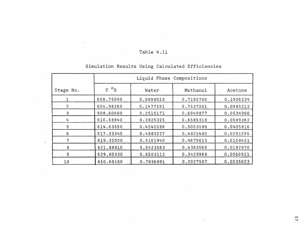
Table 4.11

Simulation Results Using Calculated Efficiencies

Liquid Phase Compositions

Stage No. T 0 R Water Methanol Acetone

1 608.75090 0.0898018 0.7195766 0.1906224

2 604.98260 0.1477591 0.7537201 0.0985212

3 608.60660 0.2515171 0.6949877 0.0534966

4 610.68840 0.2825325 0.6585318 0.0589362

5 614.63590 0.4540599 0.5053589 0.0405816

6 617.33340 0.4883227 0.4825480 0.0291295

7 619.32000 0.5161940 0.4679613 0.0158451

8 621.88810 0.5423563 0.4393568 0.0182870

9 629.89330 0.6503112 0.3429968 0.0066921

10 650.69160 0.7936891 0.2027507 0.0035603

58

V. DISCUSSION OF RESULTS

Both the theoretical and experimental results of dis­

tillation depend on a number of variables, and in some cases

relatively small deviations from the desired conditions can

cause appreciable changes in performance. This may be par­

ticularly true of variations in reflux rate, reboil rate,

and feed enthalpy. Since either a reduction of reflux

temperature from the bubble point or heat losses from a

column will affect the liquid flows from essentially all

stages of distillation, changes in these variables can also

cause variations of performance throughout a column with

appreciable overall effects.

The experimental :Murphree· efficiencies at ~orne tra.ya

have negative values as shown in Table l.j. .10. This indicates

that vapor composition has been cha~ged in a direction oppo­

site from that expected for some components along consecutive

trays. Such a situation may exist due to certain operating

factors, and they may be improved by better operating condi­

tions, such as a relocated feed tray, or by utilizing a

distillation tower more suitable for the specific separation

desired.

In validating the proposed method of calculating effi­

ciencies by comparing calculated efficiencies with efficien­

cies used in simulations, the agreement is very good as shown

59

in Tables 4.4 through 4.6. This is true because both calcu­

lation and simulation were based on the same assumptions

concerning column operating conditions.

In comparing experimental liquid compositions with the

compositions obtained from the simulation using calculated

efficiencies, Tables 4.9 and 4.11, the agreement is reason­

able in the upper trays but there is considerable deviation

in the lower part of the column. This can be partially

explained by the fact that the data used to determine

reboiler duty was not very accurate and could have introduced

some deviation from the simulation. In general, the liquid

flows throughout the column were undoubtedly different from

those calculated in determining efficiencies and those in

the simulation since there was ample opportunities for heat

losses in the reflux line and the column of the experimental

system. These errors might be expected to accumulate as the

calculation proceeds'from top to bottom of the column, and

the deviations due to erroneous flows would result in errone­

ous efficiencies. Also, the feed enthalpy was probably less .

than that indicated by temperature and this would be expected

to have a greater effect in the bottom of the column in both

calculations. Due to complex interrelations among variables

it is difficult to estimate where the errors originate, but

considering all the results, the implication is that the

experimental system is presently inadequate for reliable and

accurate estimation of distillation efficiencies. Some

60

changes which might improve the reliability would be insula­

tion of feed, reflux and reboiler lines, better insulation

of the column, and more adequate means to measure and control

feed, distillate, and bottoms flows as well as reboiler duty.

61

VI. CONCLUSIONS

With a distillation column operated at steady state,

quick, accurate calculations of stream flow rates, vapor

compositions, and component efficiencies on each plate with­

in the column were made from experimental data on liquid

plate compositions, plate temperatures, the reflux rate, and

the overall material balance. The digital computer is

essential to these computations.

As is shown in Example 4.1 and 4.2, the calculational

procedure developed in this investigation is applicable to

both hydrocarbon systems and non-hydrocarbon systems. There­

fore it should be useful for calculation of multicomponent

distillation efficiencies in many types of distillation

operations.

This study indicates that component efficiencies in the

experimental distillation system studied varied appreciably

from plate to plate. Plate efficiencies can be readily cal­

culated from experimental measurements, and a logical exten­

sion of this method could be to use chromatographic data

from a distillation unit as inputs to a digital computer to

periodically monitor efficiencies and possibly adjust condi­

tions for improved performance.

62

APPENDIX A

Analytical Procedure of Samples on Gas Chromatography

The optimum operating condition for this chromatograph

was determined by considering the many factors which have

advantageous and adverse effects on the degree of resolution

and symmetry of peak area.(3)

1. Column Temperature: A higher temperature will

reduce resolution, lower temperature has the reverse

effect.

2. Sample Size: Small sample size will improve

symmetry and resolution of peaks. But, large sample

size will increase sensitivity of detector.

3. Column Length: Longer column has better resolution

of peaks.

4. Carrier Gas Flow Rate: Faster carrier gas flow rate

will decrease sample retention time to a great extent,

but has adverse effect on detector sensitivity to a

small effect.

5. Injector Temper~ture: Too high or too low will cause

tailing peak and or leading peak.

6. Sample Injection Technique: The best technique

insures the most accurate result of analysis. It is

·important that:

a) The needle be quickly inserted its full length

through the injection seal.

63

b) The plunger be depressed as quickly as possible.

c) The needle be quickly withdrawn from the seal as

soon as the sample is expelled.

Injection seal should be prevented from leaks which may

cause baseline drift on the chart and/or sample loss.

Based on above considerations, the optimum operation

conditions are:

1. Turn on carrier gas. Adjust as 14.6 ml/min.

2. Turn on column and injector temperatures setti~g.

Set column temperature at 62°c. injector temperature

at 112°c.

3. Allow about three hours for column temperature to be

stable.

4. Adjust baseline of recorder chart according to

specific recorder manual.

5 • Sample size ranged from 0 .1 Jll to 0 . 2 Jll depending on

sample 9ompositions.

Qualitative analysis was carried out by measuring the

retention time ~f each component under identical operation

conditions. The retention time of each component using two

feet, polypak #2 packing column under the above conditions

are:

Water: 0.25 minute

Methanol: 0. 50 minute.

Acetone: 2.50 minutes

After qualitative analysis was completed, quantitative

analysis can be done for known composition samples to calcu­

late a correction factor from peak area converted to compo­

sitions.

Calculation of Correction Factors:

Standard samples of the water-methanol-acetone system

were prepared by measuring the volume (buret) of each com­

ponent in accordance with the following relationship and

density data:

ww = Pw·Vw; wm = Prn·Vm; wa = Pa·va.

Pw = 1.000 g/ml

Pm = 0.7928 g/ml

Pa = 0.7920 g/ml

at 20°c. (from "Handbook of Chemistry & Physics")

The result showed the peak area of each component did

not exactly represent the weight per cent of each component,

though closely related. The same conclusion has been drawn

by several investigators on different columns analyzed dif-

ferent systems(B, 16, 24). Therefore correction factors for

each component needed to be calculated in order to get

correct compositions.

The following table shows the result from chromatogram.

Table A-1

Correction Factors for Compositions of Water-Methanol-Acetone System

Water Methanol Acetone

True Cal. Correction True Cal. Correction True Cal. Correction

Comp. Comp. Factor Comp. Comp. Factor Comp. Comp. Factor

25.0 27.27 0.9165 50.0 52.22 0.958 25.0 20.40 1.125

33.3 35.85 0.929 33.3 34.90 0.954 33.3 29.40 1.130

50.0 54.10 0.923 25.0 26.75 0.935 25.0 19.20 1.300

80.0 82.25 0.972 10.0 10.43 0.959 10.0 7.27 1.375

10.0 11.00 0.910 80.0 82.60 0.968 10.0 6.36 1.573

25.0 28.25 0.885 25.0 "2 6. 70 0.936 50.0 . 45.20 1.108

10.0 11.84 0.845 10.0 11.80 0.847 80.0 76.30 1.050

66

APPENDIX B

Explanation of Fortran Variables and Computer Program

Fortran Variables:

1. XY is used in the computer program to denote the

composition of either liquid or vapor stream. The first

parameter denotes the phase of the stream with one (1) repre­

senting the liquid phase, two (2) representing the vapor

phase; the second parameter the stages; the third parameter

the components; the fourth parameter the number of the itera­

tion.

2. ENTH is used in the computer program to denote the

stream enthalpy, the first parameter denotes the phase

enthalpy with one (1) representing liquid phase enthalpy,

two ( 2) represe.nting vapor phase enthalpy; the second para­

meter denotes phase compositions; the third parameter the

stage temperatures; the fourth parameter the stage composi­

tions.

gram.

3. All other variables~are explained in computer pro-

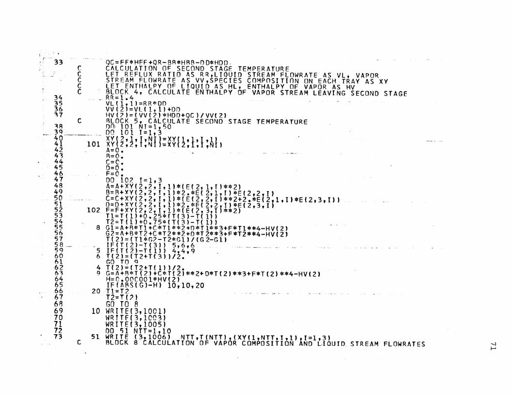
Computer Program:

(a) The calculation of condenser duty

The condenser duty is first determined from tower

operating data as shown in block 3 of the flow

chart.

67

(b) The calculation·of enthalpy of vapor stream leaving

second stage

This is calculated from tower operating data and

condenser duty determined in Step (a) as shown in

block 4 of the flow chart.

(c) The calculation of second stage temperature

With the calculated enthalpy value from Step (b),

the second stage temperature io solved from the

fourth-order algebraic equation by False-Position

Method(9). This is shown in block 5 of the flow

cha!'t.

The iterative procedure includes the following steps:

(1) The estimated second stage temperatu!'e is

first calculated from experimental first and

third stage temperatures.

(2) The second stage temperature estimated in

Step (1) is used to calculate the estimated

enthalpy.

(3) The estimated enthalpy value is compared with

the correct enthalpy value calculated in

Step (b), if the second stage tempe!'atu!'e

has been determined

(4) If the test condition is not met, return to

Step (2), using the revised value fo!' the

stage temperature.

(d) Stage-to-stage calculation of vapor composition

and internal flow rates

68

As described in Section B3 and B4 of Chapter IV,

the vapor composition is simply a function of

liquid stream flow rate. Alternately, the liquid

stream flow rate is a function of vapor composi­

tion. These functions are both first-order equa­

tions, but the function form for the feed stage is

different from that for the non-feed stage.

Therefore, it is convenient to calculate these

variables separately in the beginning of the

iterative procedure as shown in block llA, B, 13A,

B of the flow chart.

(1) The liquid stream flow rate leaving the second

stage is first assumed to be equal to that

leaving first stage which is experimentally

measured as shown in block 6 of the flow chart.

(2) Before the iterative procedure proceeds, the

first iterated value of vapor composition

leaving stage j+l is assumed to be equal to

the correct value leaving previous stage j in

order for the comparisons of the two consecu­

tive calculated values in the latter step as

shown in block 10 of the flow chart. The

vapor compositions are readily calculated

based on the assumed liquid flow rate as shown

in block llA and llB of the flow chart.

69

(3) The liquid stream flow rate is calculated

based on the vapor compositions previously

calculated by calling the enthalpy subprogram

as shown in block 13A and 13B of the flow

chart. Once the test condition is met at a

specific stage for the specific component, the

correct value of vapor composition is dupli-

cated from the last iterated value to the 50th

time.

Repeat the same procedure for all the other

components before proceeding to the next stage.

The correct value of liquid stream flow rate

is also duplicated from the last iterated

value to the 50th time before making calcula­

tions on the next stage •.

(4) At the beginning of calculation on each stage,

the vapor stream flow rate is calculated from

the correct liquid stream flow rate as shown

in blocks 9A and 9B of the flow chart.

;

- ' 1

2

:)" 4 5 6 7 8 C)

10 11 12

_13 14 15

16 17 18 lC) 20 21 22 23

.24 25 26 27 28

t 29 )f.; 30 ·- 31 •·t- ":32

.... ¥ ,,.

'4~.._ ___ ,

.-....

c c r: c c c

c

c

Efficiencies Calqulation- Program

tALCULATTON OF PLATE EFFICIENCIES FROM OPERATIONAL DATA OF TEMP. AND COMPOSITION AT STEADY ST4TE FOR CONVENTIONAL COLUMN DISTILLTNG WATER, METH4NOL, ACETON5 LET FF BE FFED RATE,DD RE DISTILLATE RATE,BA BE AOTTOM RATE,QR BE REBOILFR DUTV,QC BF CONDENSER DUTY,HFF BE FEED ENTHALPY,HDO BE DISTILLATE ENTHALPY,HBB BE BOTTOM ENTHALPY. DIMENSION XF(10l,VLC10,55),VV(10l,HV(20),Hl(20ltVEll0,3),

1PE(l0,3),XK(l0,3l,CY(l0,3),Cl(10),C2(10),C4(10),C6fl0) COMMON T(?Ol,XY(2,llt3t?Ol,Et2,4,3),N1 BLOCK 1, READ IN OPERATING DATA, EQUILIBRIUM CONSTANT ,AND ENTHALPY COEFFICIENT REAO(l,lll (T(NTTl,NTT=3tll) READ (1,12) (lXY(l,NTT,I,llti=l,3),NTT=l,ll) READ (1,13) ((E(KH,l,IJ,E(KH,2,IJ,E(KH,3,1),KH=l,2),1=1,3) RE/H) {1,14) (XF(l),I=l,3) READ (1,15) (Cl(l), C2(IJ,C4(fl,C6(1J,t=l,3) FF=3.41 00=1.12 ~R=?.2C) VV(l)=OD VL(lO,U=BA DO 16 NN=l,50

16 VLflO,NN)=Vl(lO,l) QR=38840.93 8LOCK 2, CALCULATE EXTERNAL STREAMS ENTHALPIES NI=O ... -- -----·-- ---------.--KH= 1 I<C=l NTF=ll MF=ll HFF= ENTH (KH,KC,NTF,MF) KH=l KC•l NTT=lO NTX=lO HBR=ENTH(KH,KC,NTT,NTXl KH=l KC=l T( 1 )::599.65280 NTT•l NTX•l HOO•ENTH(KHtKCyNTTtNTX) ___ ... BLOCK 3tCAL~ULATE ~ONDENSER DUTY

. ' .r --33

, .. 34 35 36 ":\7

··- ~ ~ ~ -- -

c c c c c

c

- QC = FF*HF"F +QR- BR*HRB-0 D*HDD. CALCULATION OF SECOND STAGE TEMPERATURE LET REFLUX RATIO AS RR,LIQUIO STREAM FLOWRATE AS Vl, VAPOR STREAM FLOWRATE AS VV,SPECIES COMPOSITION ON EACH TRAY AS XY LET ENTHALPY OF LIQUID AS HL, ENTHALPY OF VAPOR AS HV BLOCK 4, CALCULATE ENTHALPY-OF VAPOR STREAM LEAVING SECOND STAGE

.. RR= 1. 4 VL(l,ll=RR*OO VV(2)=Vl.(l,l)+DO HV(?)=(VV(2l*HDO+QC)/VV(2) fllOCK 5, CALCULATE SECOND STAGE TEMPERATURE

, 3~~ on. 101 NI=l,so

-~- ~r·--10~- ~~~ }! i: i !~i l=~~~ ~: 1: I :~t, 42 A=O. . 43 ~=0. 44 C-=C. 45 0=0. 46 F=O. 47 DO 107. 1=1,3 48 A=A+XV(2,2,I,U*fE(2, ltf)**2l 49 B!! R+ XV ( 2, 2, I, 1 ) * 2. *E f 2, l, J ) *E ( 2, 2{1) 50 -·------ C=C+XY(2,2,I,U*(E(2,2til**2+2.*E 2,l,Il*E(2,3,1) t 51 O=D+XY(2,2 9 1,1)*2.*E(2,2J1)*E(2,3,1) 52 102 F=F+XY(2,2,I,l)*(E(2,3ti **2) 53 Tl=T(l)+0.25*(T(3)-T(ll) 54 T2=T(l)+0.75*(T(3l-T( 1)) 55 8 Gl=A+A*Tl+C*Tl**2+D*Tl**3+F*Tl**4-HV(2) 56 G2=A+B*T2+C*T2**2+0*T2**3+F*T2**4-HV(2) 57 T(2)=(Tl*G?-T2*Gl)/(G2-Gl) . 5 8 - I F ( T ( 2 ) - T { 3 ) ) 5 , 6 , 6 .. __ _ ___ .. __ _ 59 5 lF(T(2)-T(l}) 4t4t9 60 6 T(2)=1T2+T(3))/~. 61 GO TO 9 62 4 T(2)=(T2+T(l))/2. . 6~ 9 G=A+R*T{7.)+C*Tf2)**2+D*Tf2J**3+F*T(2)**4-HV(2) 64 H=O.OOCOOl*HVf2) 65 IF(A~S(GJ-H) 10,10,20 66 20 Tl=T2 67 T2=T(?) 6R GO TO 8 69 10 WRITE(3,1001J 70 WRITF(3,1C03) 71 WRITE(3,1005l 72 DO ~1 NTT=l,lO 73 51 WRITE l3tl006J NTT,T(NTT)2CXYfltNTT,t,l)tl=l,3)

C BLOCK 8 ~ALCULATION OF VAPoR COMPOSITION AND LIOUIO_ STREAM FLOWRATES

~ --··

.74 ·7? 76 77 78 79 80 81 8?. 83 84 85 86 R7

. '- 88 89 90 91 92 93 94 95 96

97 98

99 100 101 102 103 104 105 106 107 lOR 109 110

111

112 113 114

C THROUGH WHOLE COLUMN WITH FE.EO PLATE FIXED AT 7TH DO 100 NTT=l, 11 no roo t=l,~ DO 100 NI=l,50

100 XY(l,NTT,t,NI)=XY(l,NTT,I,l) DO 200 NN=l,50 VLCl,NNJ=VL(l,l)

200 Vl(2,NNl=Vl(l,NNl NTF=?. NTL=9 NN=l NP=3 NM=l 00 104 NTT=NTF,NTL NP=NTT+l NM=NTT-1 I= 1 FT=6 IF{NTT-FT) 105 1 106,107

105 FF=O. 107 Nt=l

VVCNTT)=VL(NM,NN)+DO-FF 0!1 '3('1 J=l,3

301 XYC2,NP,J,Nf)=XY(2,NTT,J,NN) C BLOCK llA CALCULATE VAPOR STREAM COMPOSITIONS 210 DO 401 J=l,3

401 XY(2fNP,J,NI+l)=(Vl(NTT,NI)*XY(lJNTT,JflJ-VL(NM1 NNJ*XY(l,NM,J,lJ l+(VL NM,NN)+On-FFJ*XYf2,NTT1 J,NN )/{VL NTT,Nl)+uO-FF)

C RLOCK 12A CALL FUNCTION SUBROUTINE TO CALCULATE STREAM ENTHALPIES KH=2 KC=2 HVfNTT)=ENTH(KH, KC,NTT,NTTl KH=2 . KC=2 HV(NPJ= ENTHfKH,KC,NP,NPJ KH=l J<C= 1 HLCNTTl=ENTHCKH, KC,NTT,NTTJ KH=l KC=l HL(NM)= ENTH( KHtKC,NM,NMJ

C 8LOCK 13A CALCULATE LIQUID STREAM FLOWRATES VL(NTT1NI+l)=fVL(NM,NNt*CHV(NTTl-HL(NM))+OD*CHVfNTT)-HV(NPJ)+FF* l(HV(NPJ-HV(NTT)))/(HVCNP)-HL(NTT))

603 IF IABS(XV(2,NP,I,NI+ll-XY(2,NP,I,NI))-l.OE-5) 203,203,·108 108 NT=NI+l GQ TO 210

. T-115 ···· :.; 116

! 117 t 118 I 11q i 120 1-121 I 122 I 123 j 124 l 125 l. 126

127 11 128

129 I 13() 1 131

Ill fj~ 134 135

li 136 137

t 138 139

140 141 142

l44 145 14A 147 14~ 14'9 . 150 151 152

153 154 155 156

203 Nf\I=NI+l 303 XYC2,NP,I,NNJ=XY(2,NP,I,NI+l}

NN=~N+l IF (NN-50) 303,303,403

403 N"l=5C I= r + 1 IF fi-3) 603,603,103

103 CONTINUE NN=NI+l

413 VL(NTT,NN)=VL(NTT,NI+l) _ NN=NN+l IF(NN-50) 413,423,423

423 VLfNTT,~Ol=VL(NTT,49) VL(NP,l)=VL(~TT,NN) W=VL(NTT;NN) VL(Nt-1,NN =W Go Tn 104

106 VV(NTT)=VL(NM,NN)+DD FF=3.41 Nl=l VL(NTT,NI)=Vl(N~,NNJ+FF !)Q 501 J=l,3

501 XY(2,NP,J,N1)=XY{2,NTT,J,NN) C RLOCK llB CALCULATE COMPOSITION OF VAPOR STREAM LEAVING (F+lJTH PLATE

220 no 601 J=l,3 .

c c

c

601 XY(2,NP,J,NI+l)=(VL(NTTfNIJ*XY(l,NTT,JJl)-VL(NM~NNl*XY(11NM,J,l) l+(Vl(NM 1 NN)+DO)*XY(2,NT ,J 1 NN)-FF*XF(J )/(VL(NTt,Nl)+DD-rF)

RLOCK lzB CALL FUNCTION SU~ROUTINE TO CALCULATE STREAM E~THALPIES L~AVING FTH, (F+l)TH, (F-1)TH PLATES KJ..f=? KC=2 HV(NTT)=FNTH(KH,KC,NTT,NTT) -KH=2 . . KC=? HV{NPl=ENTH(KH,KC,NP,NP) KH= 1 KC=l HLCNM)=ENTHCKH,KC,NM,NM) KH= 1 KC=l HllNTTl=ENTH(KH,KC,NTTtNTT) BLOCK 138 CALCULATE FLOWRATE OF LIQUID STREAM LEAVING FEED STAGE VLINTT,NI+l)=(VL{NM,NN)*(HV(NTT)-Hl(NM)l+DO*fHV(NTT)-HV{NP))+FF*

l(HV(NP)-HFF))/(HV(NP)-Hl(NTTJ. 703 IF (A~S(XY(2,NP,t,NI+l)-XY(2,NP•I?NI))-l.OE-5) 211,211,208 208 NI=NT+l

GO TO 220 211 NN=NI+l

1 '57 158 159 160 161 162 163 1£14 165 16!, 167 166 169 170 171 172 173 174 175 176

. 177 178

. 179 . 180

181--182 1~3 lfl4 185

. 186

1.87

192 193 194 195' 196

c c

c

c

212 XV(2,MP,T,NN)=XVCi,NP,I,Nt+lJ NN=NN+-1 IF (NN-St) 212,212,410

410 "'"~=50 I= I+ 1 IF(l-3) 703,703,110

110 CONTINUE NN=NI+l

433 VL(NTT,NN)=VLlNTT,NI+ll NN=NN+l IF (NN-50) 433,443,443 ····-· ..

443 Vl(NTT,5Cl=VL(NTT,49) VLCNP,ll=Vl(NTT,NNJ V=VL(NTTJNN) VL(NM,NN =V

104 CONTINUE VV(l0)=Vl(9,50)-BB WRITEC3,1007) WRITE(3,100A) W~ITE(3,1009) DO 61 NTT-=1,10

61 WRITE (3,1010) NTTrCXYC2,NTT,I,50),1:1,3),VL(NTT,NI+l),VV(NTT) W~ITE(3,1002) QC . W~ITE(3,1004) HV(2) CALCULATION OF VAPORIZATION EFFICIENCIES AND MURPHREE PLATE EFFICIENCIES DO 17 I=l,3 VECl,IJ=l.OOOOO

, 17 PECl,IJ=l.OOOOO on 10~ NTT=2,9 00 109 l=lt3 NP=NTT+l RLOCK 1, CALCULATE EQUILIBRIUM CONSTANTS XKCNTT,Il:((((C6Cll*TCNTTl+C4Cll)*TfNTTJ+C2(l))*T(NTTl+Cl(Ill**3)

l*TCNTT) ALOCK J, CALCULATE IDEAL VAPOR COMPOSITIONS

109 CYCNTT,I,=XK(NTT,ll*XY(l,NTT,I,l) DO 209 1=1-t 3 XKf10,1)=((((C6(1)*Tt10)+C4(l))*T(l0)+C2fl))*TC10l+Cl(l))**3J

l*T(lOJ · - -__ 209 CY( 10, I l=-XK ( lQt I l *>5:(( 1, l0.1 I, 1) .. _____ . C BLOCK K~ C&LCULATE VAPORIZATION $ MURPHREE~PLATE EFFICIENCIES

00 309 I\ITT=?.,q DO 309 I= 1, 3 VE(NTT,I):XY(2,NTT,I,NNl/CYCNTT,Il

309 PE(NTT,t)=CXV(2,NTT,I,NNl-XY(2,NP,I,NN))/(CYfNTT,II-XY(2,NP,I,NN)) no 12 I=1,3 ·

'197. lqg lQ9 20C 201 202 203 204 205 206 207 208 209 210 211 212

213

214 215

216

217

218 219 220

221

222

223 224

225 226 2?7 228 229

230 231

VE(lC,Il=t.OOOOO 72 PE(1\,I)=1.00000

WRITF:C3,1011) WRITE (3,1012) WRITE (3,1013) DO 71 N TT= 1 tl 0

71 wqtTE (3,1021) NTT,CVE(NTT,J),J:l,3),(PE(NTT,JJ,J=1,3) 11 FORMAT (3Fl0.5) 12 FORMAT {3F10.7) 13 FORMATC2X,6El3.7) 14 FORMAT (1Ft0.7) 15 FORMAT(6X,4Fl4.7)

1001 FJR\1.1\T (lHl ,20X,'*OISTILLATION COLUMN OPERATING CONDITIONS*') 1002 FJRYAT (/,20X,•CONDE~SER OUTY= 1 ,5X,Fl2.4,5X, 1 BTU/MINUTE•J 1003 FORMAT (//,40X,•LIOUIO PHASE COMPOSITIONS') 1004 FQR~AT (/,20X, 1 VAPOR ENTHALPY LEAVING SECOND STAGE=•,f12.4 1 5X,

l'BTU/MJNUTEt) · 100~ FORMAT (/,lOX, 1 STAGE N0. 1 ,3X,•TEMPERATURE OR•,5X,'WATER 1 ,5X,

1 1 MFTHANOL•,5X,•ACETONE 1 ) .

1006 FJRMAT (l~X,I?,5X,Fl0.5,5X,Fl0.7,2X,Fl0.7,2X,Fl0.7 9 /l 1007 FORMAT (lHl ,20X,'*CALCULATEO OPERATING DATA FROM COLUMN OPERATING

1 CONDITIONS*'). 1008 FORMAT (//,30X, 1 VAPOR PHASE COMPOSITIONS 1 ,10X, 1 STREAM FLOWRATES•,

15X,•~OLES/MINUTE') 1009 FOR~AT (/,lOX, 1 STAf.E NO.•tl0Xt 1 WATER•,5X,•M5CH1NOL't5X,•ACETONE 1 t

llOX,'LIOUID•,5X, 1 VAPnR•l 1010 FJRMAT (]5X,T2,8X,Fl0.7,2X,Fl0.7,2X,fl0.7,7X,Fl0.7,3X,Fl0.7 9 /) 1011 FOPMAT (lHl ,zsx, 'CALCULATED PLATE EFFICIENCIES') 1012 FORMAT (/,25X,•VAPORIZATION EFFICIENCIES•,15X,

l 1 MODIFIED MURPHREE EFFICIENCUES'l 1013 FORMAT (/,lOX,•STAGE N0.•,6Xt'WATER•~5X,•METHANOL•,5X,•ACETONE 1 ,

113X,•WATER 1 ,5X,•METHANOL 1 ,5X{'ACETONt•• 1021 FJRMAT (15Xtl2t5X,Fl0.7,2XtF 0.7,2Xtfl0.7,lOX,Fl0.7,2X,Fl0.7,

12X,Fl3.7tll STOP END

FUNC.TlON ENTH(KH KC{NTT1NTXJ . . CQMMON T(?Ol,XY(i,l ,3,~Q),E(2,4,3J,NI ENTH=O. no 112 r=1,3 .

112 E~TH=ENTH+(((E(KH,3,Il*TfNTTJ+E(KH,2,Ill*TfNTTl+E(KH,l,ll)**2)* lXV(KC,NTTtltNI+ll

RETURN END

/DATA

APPENDIX C

Experimental Equipment and Operati~g ~rocedure

1. Description of Pilot-Scale Distillation Column

The major piece of equipment used in this research was

a pilot-scale distillation tower. Five components made up

the experimental distillation unit:

76

(1) Bubble-cap distillation tower: It was constructed

of brass, consisted of eight plates, 6 ~ inch in

outside diameter with six bubble-caps per plate,

and was insulated to prevent heat loss. The column

wall on the top plate was constructed of safety

. glass. Complete details are shown in Table C-1.

(2) Electrically-heated reboiler: High resistance

coils were mounted on one end of the reboiler to

supply the heat required by the distillation unit.

It was adjustable.

(3) Overhead condenser:

Type - Total condenser·, two-tube-pass, one-shell­

pass, floating-head heat exchanger. Water

was used as cooling medium.

shell diameter, inch 4.225

tube length, inch 23.5

(4). Automatic temperature recorder: Thermocouples on

each plate except the top one were used to read

temperatures. Additionally three thermocouples

Table C-1

Experimental Plates Characteristics

Tower Outside Diameter, inch 6 5 8

Tower Inside Diameter, inch 6 .

Plate Spacing, inch 6.11

Type of Plate Crossflow plate, wherein the liquid flows directly across the plate.

Round, bell-shaped cap with rectangle slots, shroud ring , and removable mounting. Six 1 inch 0, D. bubble caps on each plate, with 11

The Bubble Caps straight slots~ 0.12x0.5 inch. The total slot area is 4 inch per plate. The caps are arranged in two rows of three caps each symme-tric to the plate center and parallel to the weirs. . .

. The top plate has a circular outlet weir 1.25 inches high and 3.55 inches in circumference. Plate 2 through 8 have inlet weirs 1.125

The Weirs inches high and outlet weirs 1.25 inches high. Both weirs are straight, 4.2 inches long, and are located 7 inches from the center of the plate.

Brass pipes, 0.68 inch internal diameter, The Downcomers which reach to within 0.5 inch of the surface

of the plate below.

78

were used to measure the temperatures of feed, dis­

tillate, and bottoms. They were all electrically

connected to a temperature recorder on the control

panel.

(5) Automatic sampling device: Sampling probes were

installed in the bottom of the downcomers from ,

each plate to minimize the concentration non-uni­

formities in the liquid samples. The probes were

all electrically connected to a switch on the

control panel so that simultaneous sampling could

be done.

Accessory equipment -

(6) Feed preheater: Feed temperature was manually

adjust~d. Steam was the heating medium.

(7) Feed pump: A 1/8 hp reciprocating pump was used

to deliver the feed mixture to the distillation

unit.

(8) Recovery pump: A 1/8 hp reciprocating pump was

used to deliver the bottom product to a storage

drum and to maintain constant level of reboiler.

(9) Rotameter: A float type rotameter was used to

measure feed flow rate.

(10) Distillate divider: Three open-end glass cylinders

with graduates were used to measure reflux ratio.

It was calibrated with a curve showing relationship

of height vs. flow rates.

(11) Piping system: 5/8" schedule 40 copper tube were

used.

79

2. Description of Gas Chromatography

Gas Chromatograph consisted of four basic components(3):

(1) Carrier gas supply and flow control: Helium gas

was used as carrier medium. The cylinder reducing

valve and needle valve were used to control flow

rate of helium gas, and soap-film flowmeter was

used for measurement.

(2) Sample port: This consisted of a silicone rubber

diaphragm, loosely packed with glass wool to pro­

vide a large surface over which the liquid samples

were dispersed. A preheater consisting of a

length of insulated resistance heating wire was

wrapped about the port to insure rapid vaporization

of liquid samples.

(3) Column: Dual 1/8" diameter, 2' long stainless

steel columns were used. Polypak #2 (commercial

name of chemical of polyethylene cross-linked

polystyrene) with 60 mesh was used as packings.

Thermostatted chamber was provided around the

column to insure constant temperature in the column.

Either column could be used for analysis.

(4) Detector: The thermoconductivity detector employed

a dual, 100 ~1 volume thermistor as the resistance

element. The detector had a fixed wattage heater

that maintained the detector temperature above

column temperature to prevent condensation.

Accessory Equipment -

(5) Strip-chart recorder: This recorded the response

curve of components.

(6) Area integrator: Automatic evaluation of area

under individual response curve.

(7) Thermometer: Measured chamber temperature.

80

3. Operating Procedure for the Pilot-Scale Distillation

Column

This distillation column is operated primarily to pro­

duce engineering data such as plate temperatures, and sample

compositions, to be used in the evaluation of plate effi­

ciencies. Therefore steady state performance of the column

is desirable.

The usual precautions regarding instrument calibration

and careful measurements are made: The thermocouple on each

tray should be checked with a potentiometer; the feed rota­

meter should be calibrated by weighing the feed for a certain

period of time. Since no controller was installed, the

manipulated variables are reduced as much as possible for

steady state operation. In view of these considerations,

the following procedures for this specific design column

were followed:

(1) The continuous distillation runs begin by charging

feed storage drum and calibrating the feed rotameter

for the particular feed composition used. The feed

then is directed into the column· until the reboiler

81

is filled to a level slightly above the red line

on the reboiler sight glass. This is necessary in

order to keep the electric heater in reboiler from

burning out.

(2) Feed is then stopped, the reboiler heater is turned

on and the column is allowed to come to steady

state at total reflux. When the plate temperatures

cease changing this condition has been achieved.

This closed loop operation without feed-charge for

a pre-steady state period has several advantages:

a) The bubble point of the feed can be experimen­

tally determined. It equals to the temperature

of reboiler when bubbling vapor is first

visible on the first plate.

b) The column can achieve steady state in a

shorter time, because no outside stream could

cause a disturbance.

c) The amount of hold up on each plate, usually

difficult to measure accurately, need not to

be known, because holdup has been established

before feed enters column. Therefore the over­

all material balance, F = B + D, may be applied

throughout the steady state period.

(3) After steady state is achieved under total reflux

operation, the feed is started. The feed should be

charged to the column gradually and slowly, because

the small scale pilot plant distillation tower is

82

very sensitive to disturbances which may cause

unstable operation. It is controlled at a speci­

fied flow rate and temperature by adjusting the

steam rate through the feed preheater. The reboiler

heater is charged with constant power (i.e. con­

stant heat is supplied to the reboiler throughout

the whole period of operation). Bottoms flow is

adjusted to maintain a constant liquid level in

the reboiler. The reflux heater and/or condenser

water is adjusted to keep the reflux at the satura­

ted liquid state. The reflux ratio is adjusted to

ensure a constant reboiler level and steady column

temperature. The reflux is the only manipulated

variable. When the reflux is kept at the temper­

ature of the saturated liquid, the internal liquid

flow rate is constant. Neither condensation nor

vaporization occurs when reflux contacts the top

plate of the tower. Constant reboiler duty also

facilitates keeping the internal vapor flow rate as

constant as possible. Under these conditions

plate temperatures readily approach steady state.

(4) After feed is charged the temperatures in the strip­

ping section will be lower due to enrichment of the

heavier component in this section. (All subcooled

liquid comes down along this section.) After the

reflux is decreased from total reflux, the temper­

ature in the rectifying section will be higher due

,83

to the decrement of the lighter components in this

section. Column temperatures seemed to stabilize

in two or three hours. After that, samples from

each plate are taken. Samples are collected in

tightly stoppered glass bottles to minimize evapor­

ation prior to analysis.

( 5) Finally, the molal flow rate of bottoms and dis-

tillate are calculated by weighing during the

steady state operation period.

84

APPENDIX D

Nomenclature

a = a coefficient of the function of equilibrium constant

B = molar flow rate of bottoms product

C = number of independent components

c = a coefficient of the empirical equation proposed by

D

M E •. J~

0 E .• J~

Ev

F

f. ~

f~ ~

Prausnitz, Eckert, Orye et. al.

= molar flow rate of distillate

= modified Murphree plate efficiency

= modified vaporization efficiency

= vaporization efficiency

= reduced efficiency

= apparent efficiency

= conventional efficiency

= a coefficient of the function of enthalpy

= degrees of freedom

= molar flow rate of feed

= fugacity of component i in mixture. Superscripts L

and V refer to liquid and vapor mixture respectively.

Subscript p refers to the fugacity evaluated at total

pressure P•

= fugacity of component i in the standard state

H = enthalpy

Hp = enthalpy value evaluated at pressure p

85

= enthalpy value evaluated at zero pressure

H. J = enthalpy of one mole of the vapor leaving stage j of

a distillation column

hj = enthalpy of one mole of the liquid leaving stage j of

a distillation column -H .. = partial molar enthalpy of component i in a vapor mix­

)1

ture leaving stage j of a distillation column -h .. = partial molar entha. lpy of component i in a liquid

)1

mixture leaving stage j of a distillation column

hF = enthalpy of feed stream

hB = enthalpy of bottoms product

hD = enthalpy of distillate

K.. = equilibrium constant for component i at the tempe~a­J1

ture of stage j

P = number of phases in a system

p = total pressure. Superscripts 1 and v refer to liquid

and vapor respectively.

P = critical pressure c

Pr = reduced pressure

p. = partial pressure of component i in a mixture 1

* p. = vapor pressure of pure component i 1

Q = condenser duty c

Q = reboiler duty r

R = gas constant

= external reflux ratio at top of column

T = absolute temperature

t

T r

v -v.

l.

* v

X • • Jl.

-

= temperature. Superscripts 1 and v refer to liquid

and vapor respectively.

=

=

=

=

= =

reduced temperature

critical temperature

molar volume of pure component

partial molar volume of component i in a mixture

molar volume of pure component if it were ideal gas

mole fraction of component i in the liquid leaving

stage j of a distillation column

x = actual liquid mole fraction

x' = reduced liquid mole fraction

86

xFi = mole fraction of component i in the saturated liquid

feed

xBi = mole fraction of component i in the bottoms

XDi = mole fraction of component i in the distillate

y .. = mole fraction of component i J.n the vapor leaving Jl.

stage j of a distillation column

* in equil-y .. = fictitious vapor composition which would be Jl.

ibrium with the liquid leaving an equilibrium stage

Y. . = product of K. . and x .. , where these quanti ties are Jl. Jl. Jl.

evaluated at the actual conditions of the liquid

leaving stage j of a distillation column

y = actual vapor mole fraction. Superscript * refers to

equilibrium value.

y' = reduced vapor mole fraction. Superscript * refers

to equilibrium value.

(y) = conventional vapor mole fraction. Superscript *

refer to equilibrium value.

Greek Letters

y. = liquid phase activity coefficient of component i ].

Pw = density of liquid water

Pm = density of liquid methanol

Pa = density of liquid acetone

~ = denotes a sum

e = error limit for two consecutive iterated values

Subscripts

j = stage number

i = component number

p = constant pressure

T = constant temperature

n = stage number

87

1

2

3 4 5 6

.7 8 9

10 11 12 13 14 15 16 17 18 19 20 ?1 22 23 24 25 26 ')1 28 2Q 30 31 3? 33

Appendix E. Simulation ~r?gram Used for Checki~g Effic~ency Calculation~

.t . c c c c

c c

MAIN LINE PROGRAM---MULTICOMPONENT.OISTILLATION . COMPONENTS ARE --WATER, METHANOL, AND ACETONE DIMENSION NAME(l00)

COMMON AAA,B8R,TlL(TUL,MC,All5,4){N'NC,Tt20),SKB(20)lAK(20tl5),SV( 110),SL(20),Wf20),0 20,15l,ALP(20t 5l,AA(20,15),V(20, 5),SUMV(20),T 2HETN, . Y(20tl5l,X(20,15);TF 20),XX(20,15J,YY(20,15J,FVC20),FL-3{20),EC15,3),C(l5,3),XF(20,15 1 EF(20,70)

MC~ MIDDLE COMPONENT AS RASE, N= NO. OF TRAYS,NC= NO. OF COMPONTS READ(l,ll TLL,TUL,MC,N,NC WRITE(3,1) TLL,TUL,MC,N,NC

1 FORMAT(2Fl0.5,3I10) DO 19 I=l,NC

19 1000

lB 1005

100

REAOCl,lOOC) A(I,l),A(1,2),A(I,3JJACif4) .... --- --·-·--·-- -~ WP!TE(3,1000l A{J,l),Afi,2),A(I,3 ,A( ,4) FORMAT(6X,4El4.7) oa 18 t=t, NC REAO(l,l005) ECI 1 1JJE(I,2);Etif3);CCitll,Clli2l,C{If3)­WRITF(3tl005) E(I,l ,E(I,2 ,E( ,3 ,C(l,lJ,C( t2J 9 C( ,3) FORMATCzX,6El3.7) KK=l FORMAT(lAA4) ..

~~t~f:t3!i!~~~~li;~;!i!i~~l, 14 FORMAT(3Fl0.7)

CALL AAABRB N=N+2

1007 :~r~~1~!~8~lll~~~tl!ll!i!I~~~r~~!r~~, FORMAT(:,-,F10.7l .. _ ~UM=O READ(1,3)(T(J),J=l,N)

3 FORMAT{Fl0.5) 00 4 J=l,N ~KA(J)=FXP((AAA/T(J))+SBR)

4 CnNTTNUF. R.EAD(l,5)B,DIST

5 FORMATt2F10.3) REAO(l,6)fSV(J),SLCt),W(I),I=l,Nl

6 FORMAT(3Fl0.3l

34 35 36 37 38 39 40 41 4? 43 44 45 46 47 4A 49 50 51 52 53 54 55 56 57 58 59 60 61 6?. 63 64 65 66

67 6S3

69 70

71 72 73 74 15 76 77

RFAO(l,lr.l)(FV(J),J=l,N) 101 FOR~AT{5Fl0.5)

READ( l,lCll (Fl.(J) ,J=lrNl REAn(l,l~2)((XXCJ ,I J,I=l,NC),J=l,Nl REA0(1,102)((YVCJ ,I ),I=l,NC),J=l,N)

102 FORMAT{3Fl0.5l REAOC1,103l{TF(J),J=l,Nl

103 FORMAT{5Fl0.5) 1 ~ CAL L K C OM P

CALL ALPHA CALL A~SFAC CALL MATPAL CALL THF.TA IF(ABS(THETN-1.0)-l.E-5) 9,9,10

9 GO TO 11 10 C!JNTINlJF. 12 FORMAT{F30.6)

CALL KBASE CALL TEMPJ KK=KK+l NUM="'UM+l IF ( N lJM- 3) 13, 1 3, 3 3

33 CALL ENTHAL 87 FORMATC5X,l1Fl0.4)

GO TO 13 11 CONTJNUF

WRITE(3,38) 38 FOPMAT('l'l

DO 40 MM=l,lO R~AO(l,lOOl (NA~F(I),I=l,l8)

40 WRITE(3,100) (NAME{I),I=l,l8) WRITE(3,41) KK,THETN

41 FOR~AT(////~X,•PROBLEM CONVERGED IN 1 ,15,3X,•ITERATIONS TO A THETA 1 OF 1 ,Fl0.6)

WRITF(3,42l 42 FORMAT(////7X,•TRAV TEMPF.RhTURE VAPOR RATES LIQUID RATES

2 --------EQUILIBRIUM CONSTANTS--------•) WRITF{3,43)

43 FORMAT(3X,/5X,• l(J) SV(J) SL(J) 1 WATEP METHANOL ACETONE ,,

0!1 44 J=l,N 44 WRITE(3,45) J,T(J),SVCJ),Sl(J),AK(J,l),AK(J,2),AK(J,3) 45 FORMAT(2X,I2,2X,6Fl5.5)

14RITE(3,46) 46 FOR~AT(~X~///1,45X,•TRAY COMPOSITIONS 1 )

WRITE(3,47) 47 FOR~AT(3X,/,16X,'--------LIQUID PHASE----------- -------

1---GAS PHASE--------------•)

78 79

$l0 81 R2 R3 R4

85 c 86

87 88 89 90 91 Q2 93

c 94

95 96 97

9R 99

100

101 c 102

103 104 105 106 1C7 108

WRITE(3.,4f!) 4R FORMAT{3X•/•' WATER MFTHANOL ACETONE

1 WATER METHANOL ACETONE'} nn 49 J=t,N 49 WRYTE(3,50)J,X(J,l),X(J,2),X{J,3),Y(J,l),Y{J,2J,Y(J,3J 50 FQRMAT(/2X,I2,6Fl5.7)

CALL EXIT ENO

SUBROUTINE AAABRB

COM~ON AAA,8RB,TLLrTUL,MC,Afl5,4)rNrNC,T(~OJ,SKR(20) 1 AK(20,15),SV( llOJ,Sl(2~),W(20),0f20,1~),ALP(20,15J,AA{20,15),V(20,15),SU~V(20),T 2HETNr Y(20,15),X(20,15),TF(20),XX(20rl5),YY(20rl5l,FV{20),Fl 3(20},E(l5,3),C{l5,3),XF(20,15J!F.F(20,20) SKBU=({A(~C,l)+A(MC,21*TUL+A(MC,3)*TUL**2+ACMC,4)*TUL**3)**3)*TUL SK~l=((A(MCtl)+A{MCr2)*Tll+ACMC,3)*TLL**2+A(MCr4)*Tll**3J**3J*Tll M\A=ALOG( SKutJ/SKRL l /( n.O/TUL )-(1.0/TLLJ) BA~=-(1.0/Tll)*AAA+ALOG(SKBL) RFTliPN F.N 0 SUBROUTINE KCOMP

COMMON AAA,BBB,TllrTUL,MC,A(l5r4J,N,NC,T{20},$KB(20),AK(20tl5),SV( 11C),SL(20l,W(20),0(20,15),ALP{20ll5),AAC20,15l,V(20tl5),SU~V(20),T 2HETN, Y(20,15),X(20 1 15,,TF 20t,XXf20,15J,YY(20~15),FV(20)~FL 3(20),E(15,3),C(l5t1lrXFf2u,l5),EF(20,20) no ·5 J=lt N 0~ ~ I=l,NC ·

3 A~(J,I)=((A(J,l)+A(I,2J*T(JJ+A(I,3l*T(JJ**2+A{Ir4J*TfJJ**3)**3)*T( lJ,

5 CONTINUE RETURN ENO

SUBROUTINE ALPHA

f.O~MrN AAA,~BR,TLL,TUL,~C,AC15 1 4J,N,NC,T{20t,SKB(20l,AKC20tl5) 1 SV( 11Ql,Sl(l0),W(20),0. C20,15),ALP{~Ofl5),AA(20,15) ,V(20,15),SUMV(2U),T. 2HETN, YC20115),X(20,15J,TF 20JrXX(20,15),YY(20 9 15),fV(20),Fl 3(20t,EC15,3),C(l~,~),XFC20,15),EF(20,20)

00 5 J=lrN Oil 3 I= 1, NC

3 ~LPCJ,IJ=AK(J,IJ/SKB(J) 5 CONTINUE

RETURN END

(.0

0

lQq

110

111 112

113 114 11? 116 117

llR llq 120

121 122 12~ 124 125 176 127 12A ]2Q 130 131 132 133 134 135 136 137 138 139 140 141 142 143 144 145

c

c c

c

SU~ROUTINE ARSFAC

COMMON AAA,RBR,TLL,TIJL,MC,A(l5,4),N,NC,T(20),SKBf20),AK(20tl5),SV{ llO),Sl(20t,Wf20),0(20,15),ALP(20,15),AA(20,15),V(20,15J,SUMV(20),T 2HETN, YC20,15),X(20,15),TF(20),XX(20,15),VY(20tl5),FV(20),Fl 3(20),E(l5,3),Cfl5,3),XF(20,15J,EF(20,20) no 10 J=l,N DO R I=l,NC TOTAL CO~DENSER HAS A K = 1.000 AK (l ,r )=1 .0

8 AA(J,l)=Sl(J)/tAK(J,Il*SV(Jl*EF(J,IJJ 10 CONTINUE

RETURN END

SUBROUTINE MATBAL DTMENSIO~ F(20),G(20) . CO~MON AAA,B9RtTlltTUliMC,At15,4)lN'NClTI20J 1 SKBf20)lAK(20,15)!SVf

~~~+~~Lc 2 oJ,wt~~b!~~f~ltib:th~!f~tz8J:~x~.~8:l~J:~~f~b,~&I~~~Y~~~!~[ 3(20J,E(l5,~),C(l5,3),XF(20t15J,EFC20 1 20) N=N-1 DO lCO J=·t,N OIJ lCO T=I,NC O(J,Il=-XXCJ,I)*Fl(J)-FV(J+ll*YV(J+l,IJ OflOfJ)•O.C .

100 CONT NUF N=N+l no 11 1•1 1.1\JC 1)11 A J:},N IFCJ-1)1?1.3

l ~lll= -1./(l+AA(J,tll G( lJ=FfU*f)(J.,l) ·- _... GO TO 8

3 FCJJ=l./(-(l.+AA(J,I))-AA(J-l,I)*Cl.-W(J)/SL(JJ)*FCJ-1)) GfJ}=(£'CJ, I )-AA(J-ltl )*(1.-W(J)/SL{J) l*GlJ-U )*F(J)

A C:f'JNTINUE 1)0 Q l=l,N IF(l-112t2!4

2 VCN,l)•G(NJ GO TO q

4 V(N-L+1,I)•GfN-L+ll-F(N-L+l)* VCN-L+2,IJ 9 CONTINUE ll CONTl~UE

RFTURN END

i46 ·C

SUf'ROlJTI~E THFTA

·147 DIMENSION DC0(20l,RC0(20J · . 148 COMMON AAA,R8R,TlltTUL,MC,A(l5,4),N,NC,Tf20),SK8(20) 9 AK(20,15J,SV(

c

llOJ,Slf20),W(20),D(20,l~J,ALP(20,15),AA(20tl5),V(20~15),SUMVf20),T 2HFTNt Y(20~15),X(20,15JJTF(20),XX(20,15),YY{2Utl5),FV(20),Fl 3(20), E( 15,3) ,C( 1!:>,3), XF( 20,15 ,EFC 20 9 20)

C FOR THIS PROBLE~ F = 3.41 149 FDT=3.41 150 THFT=O.O 151 2 SUT=C.O 152 OSU~=O.O 153 00 lP I=l,NC 154 ~DC~=V(N,I>*AA(N,IJ/V(l,IJ 155 SUT=SUT+FDT*XFC1,3)/( l.O+THET*BDCA) 1'56 DSlJM=OSUM-BDCA*fDT*XF(l,3)/(l.O+THET*ROCA)**2 157 10 CONTINUE

C. C FOR THIS PROBLEM D = 1.120

158 THETN=THET-{SUT-1.1201/0SUM 15Q IF(ABSfTHETN-THET)-2.E-5)1'5,15,20 16C 15 CaNTINUE 161 GO TO 40 162 20 THET=THFTN 163 GO TO 2 164 40 00 50 I=l,NC 165 DCO(J)=FOT*XF(J,3)/(l.+THETN*V{N,I)*AA(N,IJ/V(l,l)) 166 50 RCO(T)=THETN*CV(N,Il*4A(N,I)/V(l,I)l*DCOfl) 167 DO 60 J=l,N 168 SUMV{J)=O.O 16q SLSUM=O.O 170 SVSUM=C.O 171 DO 55 I=l,NC . 172 SVSUM=SVSUM+CV(J,IJ/V(l,I))*DCO(I) 173 SL SUM=SL SUM+ ( AA( J, t l *Vf J t t) /V ( 1 t IJ) *OCOti) 174 G~ TO ~5 175 WRITEf3,1112) I,SLSUM,SVSUM 176 1112 FORMATf6X,I4t'L=•,FI0.3, 1 V= •tF10.3) 177 55 SUMV(J)=SUMV(J)+V(J,I)

I+~ ~?J;y,!{l!~S,I)*VIJ,I)*DCO(l)/V(l,J))/SLSUM 180 YfJtiJ=((VfJ,l)/V(l,I ))*OCO(I)J/SVSUM lAl 56 CONTINUE lR2 60 CONTINUE lS~- · RETUPN 184 ENO

:-1A5 S!Jf\ROUTINE'KBASF

c 186 DIMENSIO~ SUM(20) 187 COMMON A~A,8BR,TLL,TUL,MC,A(l5,4),N,NC,T(20),SK8(20l,AK(20,15l,SV(

11Cl,SL(20),W(20),0{2C,l~),ALP(20,15),AA(20tl5),V(20tl5ltSUMV(20),T 2HfTN, Y(20,15),X(20,15l,TF(20l,XX{20,15),YY(20,15l,FV(20),Fl 3{20),E(l~,~l,Cfl5,3),XF(20tl5l,EFC20,20)

188 00 5 J=l,N l 189 SUM(J)=O.O .; 190 on 3 r=l,NC

·191 3 SUM(J)=SUM(J)+(X(J,l)*ALP{J,Il*EF(J,!)) 192 SKA{J)=l./SUM(J) IQ3 5 CONTINUE 194 RETURN 195 END

lC~6 SUBROUTINE TEMPJ c 197 COMMON AAA,BBR,TLL,TUL,~C,A(l5,4),N,NC,T(20),$KBC20),AK{20,15l,SV(

110),Sl(20},W(20),0(20,15l,ALP(20,15l,AA(20,15),V(20,15l,SUMV(20),T 2HETN, Y(20,15),X(20,15),TF(2Q),XX(20,15l,YYf20,15),FV(20J,Fl 3{20),E(l5,3),C(l5,3),XF(20tl5),EFf20,20)

l9R 00 6 J=l,N 1Q9 T(JJ=AAA/(AlOG(SKA(J))-BBB) 200 WRITF(3 1111) J,T(J) 201 1111 l=nRMAT(~X,I4,•TEMP:= 1 ,Fl0.3) 202 6 CQNTtNUF 203 RETURN 204 END

205 SUBROUTINr:: ENTHAL c

COMMnN AAA,RBR,TLL,TUL,~C,A(l5,4),N,NC,T(20),SKB(20),AK{20,15),$V( 206 110),SL(20J,W(20ltOC20t15JtALP(20,l?),~Af20,l5),V(20,15l,SUMVC20l,T ?~FTN, Y(20,15),X(20,15JJTFC2C),XXC20tl5J,VY{20,15),FV(20),Fl 3(20l,E(l?.3),C(l5,3),XF(20,15 OEF(20,20)

207 DTMENSIO~ Hf20215)EHHC20zl5J,T TH(20l,HFL(20l 0HFV(20),f.NTH1(20t,EN 1TH2(?0),F~TH4( Olt ~TH5( OJ,ENTH6(20l,TOTHH(2 )

20J3 no ?tt J=I,N 209 DO 24 I=l,NC ?10 H(J,IJ=llCCt ll+CCI,2l*T(J)+C{I 3l*T(J)**2l**2l 211 HH(J,TJ=ffECi,lt+E(J,2l*TfJJ+Eif,3l*TfJ)**2l**2) 212 24 CONTINUE 213 26 CONTINUE 214 00 1 J=l, N 215 HFL(J);;;Q.O

CD w

21A 217 218 219 220 221 222 223 224 ?.25 226 277 228 229 230 231 /32 233 234 2?'5 236 237 ?38 239 240 241 242 243 244 24S 246 247 24~ 249

c c 250 251

.252 ?153 254

2'5'5 256 257

FITHH( J )=0.0 TOTH(J)=O.O HFV(J)=C.C on 2 I=J,NC TOTH(JJ=TQTH(J)+H(J,I )*X(J,I, TOTHH(J)=TOTHH(J)+HH(J,IJ*V(J,J) . HFL(J)=HFL(J)+f(Cfltl)+C(I,2J*TF(JJ+C(J,3)*TF(J)**2)**2)*XX(J,I) HFV(J)=HFV(J)+((ECI,lJ+E(I,2J*TF(JJ+E(I,3J*TF(JJ**2)**2)*YY(J,I)

2 CONTINUE 1 CONTINUJ::

N;:;:N-1 DO 3 J=l,N ENTHU J)=O.O E"JTH5(J)=O.O ENTH6(J)=O.O . DO 4 I=l,NC ENT4l(J)=ENTH1(J)+HH(J+l,I)*VCJ,J) ENTH5(J)=ENTH5(J)+HH(J+l,IJ*XX(Jti) ENTH6{J)=FNTH6(J)+HH(J+l,I)*X(J,I)

4 CONTTNIJE 3 CONTINUE

O'J 5 J-=2,N ENTH2(JJ=O.O 00 6 l=l,NC ENTH2(J)=FNTH2(J)+HH(J+1 1 I)*X(J-l,J)

6 C'1NTINUE 5 CO~TINtJF

00 7 J=ltN ENTH4(Jl=O.O 00 13 f=l,NC E~TH4(J)=ENTH4(J)+ H~(J+l,I)*YY(J+l 1 1)

8 COI\ITINLIF 7 C'lNTINUE

00 q J=?,l\l

FLOW RATES FOR THIS PRO~LE~ ONLY SVtlJ=l.l20 SV(2)=2.688 SL(ll=l.568 SLC1CJ=2.290 SL(J)=(SV(J)*(~NTHl(JJ-TOTHH(J))+(W(J-l)-SL{J-l)l*tENTH2(JJ-TOTH(J

l-l)l+FV(J+l)*(HFV(J+l)-ENTH4(Jl l+FL{J)*{HFL(JJ-ENTH5(J)))/(TOTH(J) 2-ENTH6(JJ l SV(J+l)=~V(J)+Sl(J)-SL(J-l)+W(J-1)-FL(J)-FV(J+l)

9 CONTINUE 69 FORMAT(2X, 1 SL(J)=•,F20.5!5X,•SV(Jl= 1 tF20.5)

258 25q 260 261 262 263 264 265

266 267

26A 269 270 271

N=N+l 00 10 J=l,N WRITE(3,69)$l(J),SV(J)

10 CONTINUE CDNO=(TOTHH(2l-TOTH(l))*SV(2) RESOIL=Sl(N-l)*TOTH(N-1)-SV(Nl*TOTHH(NJ-SL(N)*TOTH(N) WRITE(3,52l TOTHH{2),TOTH{l)

52 FOR~AT(/2X,•VAP. ENTH. OFF 2 = 1 tF12.3,2X,•LtQ. ENTH. OFF 1 =1 ,Fl2. 13) W~ITEf3,5ll CONO~RE~OIL

-~51 FORMAT(//5X, 1 CONuENSER DUTY =·,~~?·2t' ST~/HR.•,5Xt'REBQILER DUTY

1~• 1 Ft2.2i' BTU/HR.~/) WR TE(3, lHHETN

ll FORMAT(Fl0.7) ... _ RETURN END

96

BIBLIOGRAPHY

1. A.I.Ch.E., Bubble Tray Design Manual, pp. 26-40.

2. Davis, Taylor, and Holland, A.I.Ch.E. Journal, pp. 678-681, July, 1965.

3. Dal Nogare, Juvet, Gas-Liquid Chromatography, Inter­science Publishers, 1962.

4. Diener, Gerster, Ind. Eng. Chern., Process Design and Development, July, 1968.

5. Drickamer, Bradford, Trans. Am. Inst. Chern. Eng., v. 39, p. 319, 1943.

6. Gerster, Mizushina, Marks, and Catanach, A.I.Ch.E. Journal, December, 1955.

7. Gilliland, E. R., and Reed, C. E., Ind. Eng. Chern.~' No. 5, pp. 551-557 (May, 1942).

8. Grob, Mercer, Gribben, and Wells, Journal of Chromato­graphy l' p. 545 (1960).

9. Holland, Multicomponent Distillation, Prentice-Hall, 1963.

10. Holland, and Welch, Petroleum Refiner, 36, No. 5, 1957, pp. 251-253. --

11. Kastanek, and Standart, Separation Science, 1967, pp. 439-486.

12. McAdams, Perry, J. H., Chemical Engineers' Handbook, 3rd edition, pp. 582-583.

13. McCabe, W. L., and Thiele, E. W., Ind. Eng. Chern. 17, p. 605 (1925).

14. Murphree, Ind. Eng. Chern. 17, pp. 747-750 (1925).

15. Nord, Trans. of A.I.Ch.E. 42, p. 863 (1946).

16. Nunez, Armstrong, Cogswell, Analytical Chemistry, ~' p. 1164 (1957).

17. O'Connell, Trans. of A.I.Ch.E., 42, p. 741 (1946).

18. Perry, J. H., Chemical Engineers' Handbook.

19. Petroleum Refiner, January, 1949, p. 87.

20. Petroleum Refiner, November, 1949, p. 127.

21. Petroleum Refiner, September, 1950, p. 136.

22. Petroleum Refiner, August, 1951, p. 120.

23. Prausnitz et. al., Computer Calculations for Multicom­ponent Vapor-Liquid Equilibria, Prentice-Hall, 1967.

24. Schomburg, G. Z., Anal. Chem., 164, p. 147 (1958).

25. Smith, B. D., Design of Equilibrium Stage Processes, McGraw-Hill, 1963.

26. Smith, J. M., Introduction to Chemical Engineering Thermodynamics, 1959.

97

2 7. Waggoner, R. C. , Jones, J. H. , "Distillation Simulation Program" (personal communications).

ACKNOWLEDGEMENTS

The author is indebted to Dr. Raymond C. Waggoner,

Associate Professor of Chemical Engineering, who suggested

this investigation and served as a research advisor. His

help, guidance and encouragement are deeply appreciated.

98

Grateful thanks is extended to Dr. Marshall E. Findley,

Associate Professor of Chemical Engineering, for his advice

and help towards this thesis.

The author is much indebted to Dr. Virgil J. Flanigan,

Assistant Professor of Mechanical Engineering for his con­

structive comments on the writing of this dissertation.

The assistance of Mr. James H. Jones, graduate student

of Chemical Engineering in checking computer program, and

Mr. C. L; Yeh and Mr. Paul Chiang, both graduate students of

Chemical Engineering, in doing the experimental work are

gratefully acknowledged.

Dr. Russell A. Primrose, and Professor Jerry J. Carr who

provided the experimental equipment for this research deserve

a great deal of thanks.

Finally, the author wishes to thank his parents for

their constant help and encouragement. Their contributions

are too many to enumerate.

99

VITA

The author, Cherng Shyong Wang, was born on January 26,

1938 at Tainan, Taiwan_, Republic of China. He attended

elementary school and high school at Tainan. The author

joined National Taiwan University in 1958 and obtained a

B. S. Degree in Chemical Engineering in 1962. He then served

in the Chinese Army Reserve for one year as a second lieuten-

ant. He worked for Mobil China Allied Chemical Industries,

Ltd at Miao-li, Taiwan from 1963 to 1965. He became a grad-

uate student in the Chemical Engineering Department of the

University of Missouri-Rolla in September, 1965.