Determination of payback periods for photovoltaic systems in domestic properties

O'FLAHERTY, Fin <http://orcid.org/0000-0003-3121-0492>, PINDER, James and JACKSON, Craig

Available from Sheffield Hallam University Research Archive (SHURA) at:

http://shura.shu.ac.uk/5667/

This document is the author deposited version. You are advised to consult the publisher's version if you wish to cite from it.

Published version

O'FLAHERTY, Fin, PINDER, James and JACKSON, Craig (2012). Determination of payback periods for photovoltaic systems in domestic properties. In: Retrofit 2012, Salford, UK, 24-26 January 2012.

Copyright and re-use policy

See http://shura.shu.ac.uk/information.html

Sheffield Hallam University Research Archivehttp://shura.shu.ac.uk

Determination of payback periods for photovoltaic systems in

domestic properties

Fin O'Flaherty1, James Pinder

2 and Craig Jackson

3

1Centre for Infrastructure Management, MERI, Sheffield Hallam University, S1 1WB, UK 2Visiting Fellow, Sheffield Business School, Sheffield Hallam University, S1 1WB, UK 3South Yorkshire Housing Association, 43-47 Wellington Street, Sheffield, South

Yorkshire, S1 4HF

Email: f.j.oflaherty@shu.ac.uk, j.a.pinder@shu.ac.uk, c.jackson@syha.co.uk

Abstract:

The paper reports on the two year performance of photovoltaic (PV) systems which

were installed on 23 new build properties in South Yorkshire, UK, and the impact of the

feed-in-tariff on payback periods. The majority of the properties (17 No.) were fitted

with a 3.02 kiloWatt peak (kWp) photovoltaic system, designed to supply, on average, up

to 2400 kiloWatt hours (kWh) of solar energy per annum whereas the remaining six

systems were 3.75 kWp systems providing, on average, up to 3000 kWh per annum. The

photovoltaic panels were integrated into the roofs at the time of construction. Datum

readings were taken during commissioning in Summer 2007 with subsequent readings

taken as close as possible to the second anniversary in 2009.

A discounted cashflow model was developed which determined payback periods based

on actual and assumed performance and different economic scenarios. A comparison is

made between the Renewable Obligation Certificate (ROC) and the Feed-in-Tariff (FiT)

schemes in determining payback periods. Huge variations in payback periods are shown,

for example, a poorly performing 3.02 kWp photovoltaic system irrespective of quantity

of electricity used in the home will take in excess of 100 years to payback under the ROC

scheme. The same system under the FiT scheme with 25% electricity exported to the grid

would have a payback period of 66 years. However, if the same system performed to its

designed specification, the payback period would decrease to 16 years. This highlights

the need of ensuring the photovoltaic systems are working to their full potential and that

householders are fully aware of how to get the best from their systems.

Keywords:

energy generation, feed-in-tariff, payback period, photovoltaics, renewable obligation

certificate

1 Introduction

Approximately 27 percent of energy used in the UK is due to the housing sector

(Department of Trade and Industry, 2006). Renewable energy technologies, such as solar

photovoltaics (PV), offer an opportunity to reduce carbon dioxide (CO2) emissions from

homes and contribute to the Government's target of generating 15 percent of the UK's

energy supplies from renewable sources by 2020 (DECC, 2009).

However, an area of concern is the time taken for these technologies to pay for

themselves. This paper investigates the payback period for PVs in domestic housing and

focuses on an Eco-Homes development in South Yorkshire, UK. The development of 23

three-bedroom affordable homes with state of the art renewable energy technologies was

completed in September 2007. All homes are fitted with solar PV and solar hot water

systems. The performance of the PV systems will be presented in this paper only.

Electricity generated from the PV systems is immediately used by the residents ahead of

grid electricity. Surplus electricity is exported back to the grid. Residents have the

opportunity of selling the surplus energy to their supplier in the form of Renewables

Obligation Certificates (ROCs) as this was the scheme in place at the time of installation.

This has since been replaced by the feed-in-tariff and the paper will compare the payback

periods for both schemes.

2 Research Significance

The 2006 review into the sustainability of existing buildings (Department for

Communities and Local Government, 2006) found that 152 million tonnes of carbon

(MtC) were produced by the UK in 2004. In total, 27% of this figure was attributable to

the domestic building stock, or 41.7 MtC. Domestic emissions will have to fall by 24.7

MtC to 17 MtC by 2050 if the domestic sector is to reduce in line with overall carbon

emissions targets. In addition, The Stern Review (Stern, 2006) predicted that, due to

climate change, there will be less cold related deaths in the winter but more heat related

deaths in the summer. As a result, gas consumption will decrease in the winter but due to

an increased use of air conditioning in the summer months for cooling, electricity

consumption will increase (Department for Communities and Local Government, 2006).

Regardless, the onus remains on the use of renewable energy technologies to reduce

domestic building stock emissions and the results presented in this paper will help

determine PV has the potential to generate renewable energy at an affordable price.

3 Research Methodology

Three different design of properties exist in the development. A total of 8 properties

were fitted with a 3.02 kWp photovoltaic system (fifty eight PV tiles) on a roof pitch of

40. Nine other properties had a similar photovoltaic design except the roof pitch was

27. Finally, six properties were supplied with a 3.75 kWp photovoltaic system (seventy

two photovoltaic tiles) on a 27 pitch.

The energy generated from the photovoltaic panels was manually monitored using the

household kWh electricity meter. Electricity meter datum readings were taken upon

commissioning the systems in August or September 2007. Final readings taken as close

as possible to the second anniversary of the commissioning two years later.

4 Findings and Discussion

4.1 Solar PV performance

Table 1 gives details of the solar PV systems and energy generated over the two year

monitoring period. The property identification is given in col. 1. The solar energy

generated is given in col. 2, Table 1. Two roof pitches were used in the design of the

properties (27 and 40) and these are shown in col. 3. Col. 4 shows if the roofs were

subjected to shading. The monitoring duration for each property is given in col. 5 and

varies slightly due to the inability to gain access to some properties for the second

anniversary readings. Comments on the performance of the systems are given in col.6.

Referring to Table 1, col. 2, the best performing PV system generated 5717 kWh during

the monitoring period whereas the worst system generated only 1512 kWh. In addition,

five of the 3.75 kWp systems (I, Q, K, R, L) performed reasonably well in relation to the

other properties and occupy five of the top eight positions in Table 1. However, system U

is also a 3.75 kWp array and performs less well, but others reasons are responsible for its

Table 1: PV monitoring data for case study 2

1 2 3 4 5 6

ID Solar

Energy

(kWh)

Roof

Pitch

()

Shad-

ing

Time

(yrs)

Comments

I* 5717 27 no 2.04

Q* 5367 27 no 2.03

F 4927 40 no 2.08

K* 4852 27 no 2.04

A 4649 40 no 2.15

R* 4318 27 no 2.03

T 4275 27 some 2.03

L* 3718 27 no 2.04

O 3228 27 some 2.04

H 3206 40 no 2.02 Vandalism to power supply, Mar-Jul 09

P 3191 27 some 2.04

C 3177 40 no 2.03 Encountered grid supply turned off, 15/7/09

D 3163 40 no 2.04

G 2541 40 no 2.03

N 2535 27 some 2.04

E 2436 40 no 2.03

J 2427 27 some 2.04

S 2244 27 some 2.03

W 1827 27 some 2.03

U* 1815 27 no 2.07 Encountered PV switched off, 15/7/09

V 1785 27 some 2.03 Encountered PV switched off, 8/4/09

B 1515 40 no 2.04 Not operational Jan-Aug 09, switched off

M 1512 27 some 2.04 Inverter not operational, Jul-Aug 09

* indicates 3.75 kWp, otherwise 3.02 kWp

poor performance as described below. The 3.75 kWp arrays were designed to provide,

on average, 3000 kWh of energy per annum (6000 kWh over two years) but none of 3.75

kWp systems met this specification.

The 40 roof pitches are all fitted with 3.02 kWp systems and are shade free. However,

their performance varies considerably, property F having the third best performing

system and was the only array to exceed the design specification (4927 kWh over two

years as opposed to the design specification of 4800 kWh). However, six of the nine

properties which were categorized by the designer as being shade affected exhibited a

performance at the lower end of the table, occupying six of the lowest nine positions in

Table 1. These properties also exhibit a 27 roof pitch. Shade affected properties T, O

and P performed better (also 27 roof pitch). Properties H, C, U, V and B all suffered

operational problems within the final quarter of monitoring (Table 1, col.6) and

unsurprisingly, occupy the last four positions in Table 1. For example, the PV arrays in

properties U, V and B were inexplicably switched off for an unknown length of time

within the final seven months of monitoring, with the residents not knowing why this had

happened. This highlights the need for proper training or coaching for residents to help

them gain maximum benefit from living in a home fitted with renewable energy

technologies. The external power supply to unoccupied property C was switched off for a

period of time. This was also the case for unoccupied property H, due to vandalism of the

mains power supply. Property M did not exhibit an increase in meter readings in the final

month of monitoring. These operational issues had a bearing on the output from the PV

arrays and obviously influenced their performance.

Irrespective of the reasons for the varied performances, the focus of the paper will be on

the payback period for two of the PV systems described here. It will enable private

investors, scheme funders or housing associations to make more informed decisions on

whether or not to install PV as part of their development strategy and takes into account a

number of different performance scenarios as presented in the following section.

4.2 Solar PV payback analysis

Renewable Obligation Certificate

Solar PV performance data for two of the above properties (N and L) were used to

undertake a payback analysis. These two properties were selected on the basis that they

were neither the best or worst performing systems. The purpose of the payback analysis

was to:

- determine how long it would take for the PV systems to pay for themselves under

different economic conditions;

- compare the payback periods based on assumed and actual performance data, so as to

determine the financial cost of system under-performance.

The first stage of the payback analysis involved constructing a discounted cashflow

model using specified annual PV performance data, that is to say the electricity that

would be generated by the solar PV systems if they were operating to their design

specifications. For the 3.02kWp system (property N), the specified annual output was

2,416kWh and for the 3.75kWp system (property L) it was 3,000kWh. The main

assumptions included in the model were as follows:

- avoided electricity cost: 14p/kWh - export electricity tariff: 14p/kWh

- degradation rate of PV: 0.5%/yr - interest/discount rate pa: 5%

- Increase in electricity prices pa: 5%

- export tariff income increase pa: 0%

- inverter replacement every 10 yrs: £450

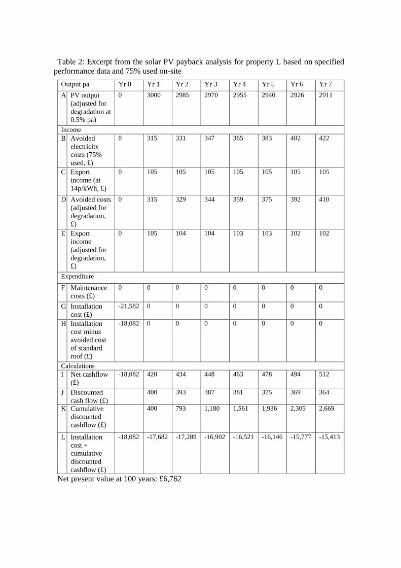
An excerpt from the payback model using assumed data for Property L is shown in

Table 2 (covering the first seven years only due to space restriction). The payback model

comprises:

- the annual output of 3,000 kWh for PV system in Property L, which was estimated to

degrade by 0.5% per year (Table 2, Row A)

- the avoided electricity costs to the residents, that is to say the cost of the electricity that

the residents would have drawn from the grid if they were not using electricity from the

solar PV system. Given that it is unlikely that residents would use all of the PV generated

electricity, three different scenarios were devised in which residents used either 25, 50 or

75 percent of the electricity generated. The cost of electricity was estimated to be

14p/kWh and this was increased annually by an inflation factor of 5 percent. The

example in Table 2 assumes 75% was used in the home (Table 2, Row B)

- the export income generated by the solar PV system, based on an assumed export tariff

of 14p/kWh and modelled using the three different scenarios described above. The export

income was not subject to an annual inflation factor, however, the impact of changes in

the export tariff can have on the payback periods of the solar PV systems will be

discussed below (Table 2, Row C)

- both the avoided electricity costs and export income were adjusted to account for

degradation of the solar PV performance over time (Table 2, Rows D and E)

- maintenance costs are assumed to be 0 (except for replacing the inverter every 10

years, Table 2, Row F)

- the capital cost of buying and installing the solar PV systems (£18,010 for the

3.02kWp system, £21,582 for the 3.75kWp system). Since the PV systems were roof

integrated, the avoided capital of a standard roof covering (estimated to be £3,500) was

subtracted from the installation cost, to give a final installation cost of £14,510 and

£18,082 respectively (Table 2, Rows G and H).

- annual net cashflows were calculated by subtracting the total annual expenditure from

the total annual income (Table 2, Row I). The present value of each annual net cashflow

was then calculated using Equation 1 (Table 2, Row J), in order to reflect the time value

of money.

Equation 1 where:

PV = net present value r is the discount (or interest) rate

CF = is the net cash flow (annual income

– expenditure) at time t

t is the time of the cash flow (i.e. year 1,

year 2 etc…)

- the cumulative discounted cashflow (Table 2, Row K) was calculated by adding each

successive discounted cashflow over the analysis period (100 years). The capital cost of

the solar PV system was then subtracted from the cumulative discounted cashflow in

each year of the analysis period, in order to determine the payback on the initial capital

investment (Table 2, Row L).

P VC F

(1 r ) t

Table 2: Excerpt from the solar PV payback analysis for property L based on specified

performance data and 75% used on-site

Output pa Yr 0 Yr 1 Yr 2 Yr 3 Yr 4 Yr 5 Yr 6 Yr 7

A PV output

(adjusted for

degradation at

0.5% pa)

0 3000 2985 2970 2955 2940 2926 2911

Income

B Avoided

electricity

costs (75%

used, £)

0 315 331 347 365 383 402 422

C Export

income (at

14p/kWh, £)

0 105 105 105 105 105 105 105

D Avoided costs

(adjusted for

degradation,

£)

0 315 329 344 359 375 392 410

E Export

income

(adjusted for

degradation,

£)

0 105 104 104 103 103 102 102

Expenditure

F Maintenance

costs (£)

0 0 0 0 0 0 0 0

G Installation

cost (£)

-21,582 0 0 0 0 0 0 0

H Installation

cost minus

avoided cost

of standard

roof (£)

-18,082 0 0 0 0 0 0 0

Calculations

I Net cashflow

(£)

-18,082 420 434 448 463 478 494 512

J Discounted

cash flow (£)

400 393 387 381 375 369 364

K Cumulative

discounted

cashflow (£)

400 793 1,180 1,561 1,936 2,305 2,669

L Installation

cost +

cumulative

discounted

cashflow (£)

-18,082 -17,682 -17,289 -16,902 -16,521 -16,146 -15,777 -15,413

Net present value at 100 years: £6,762

- the net present value (i.e. the present worth of all the cashflows) at 100 years (Table 2,

footnote) was calculated by taking the sum of all the annual discounted cashflows and

subtracting the capital cost of the solar PV system.

Figure 1 shows the estimated payback period for the solar PV system in property N,

based on the above assumptions and working at its design specification. The cumulative

discounted cashflows for the three different scenarios suggest that the solar PV system

has a very long payback period, although the time taken to break-even (when the

cumulative cashflow becomes positive) on the initial investment varies depending on

what proportion of PV generated electricity is used on-site or exported to the grid. For

instance, the payback period is 67 years when 75 percent of the PV electricity is used on-

site, but in excess of 100 years when only 25 percent of PV electricity is used on-site.

However, even if a 5 percent inflation factor is applied to the export tariff, the payback

period is still 54 years, which is clearly longer than the design-service life of the PV

system. Figure 1 also shows the payback period of the solar PV system in property N

based on its actual performance over the two year evaluation period. The annual output

of the system (based on its average performance over two years) was 1268kWh, which

means that the system was performing at 52 percent of its design performance. The

cumulative cashflows for all three electricity consumption scenarios indicate payback

periods in excess of 100 years. Even when the export tariff is inflated by 5 percent per

year, the payback period under all three scenarios remains in excess of 90 years. This

highlights that impact that under-performance can have on the cost-effectiveness of solar

PV systems. Indeed, even when the export tariff is inflated by 5 percent per year, every

10 percent decrease in system performance results in a 7.5 year increase in the estimated

payback period.

Figure 1: Solar PV payback periods for property N (3.02 kWp) based on specified and

actual performance and different electricity consumption scenarios

-£20,000

-£10,000

£0

£10,000

£20,000

£30,000

0 10 20 30 40 50 60 70 80 90 100

Cu

mu

lati

ve d

isco

un

ted

cas

hfl

ow

Year

75% used / 25% export (specified) 75% used / 25% export (actual)

50% used / 50% export (specified) 50% used / 50% export (actual)

25% used / 75% export (specified) 25% used / 75% export (actual)

Figure 2 shows the payback periods based on the specified and actual performance of

the solar PV system in property L (a higher output and better performing solar PV

system). When the PV system is assumed to be operating at its design specification and

75 percent of PV electricity is consumed on-site, the payback period is 66 years, although

this falls to 53 years when the export tariff is inflated by 5 percent per year. However,

when the PV systems actual annual output (1859kWh or 62 percent of its design

specification) is input into the model and even with a 5 percent inflation factor on the

export tariff, the payback period increases to 96 years. Under these conditions, the PV

system would generate a net financial saving of £260 in the first year of operation and

cumulative net savings of £5,393 (net present value) in the first 25 years of operation

('savings' refer to the net discounted cashflow comprising of income and avoided costs).

By contrast, the smaller capacity and poorer performing PV system in property N would

generate a net financial saving of £177 in the first year of operation and cumulative

savings of £3,535 (net present value) in the first 25 years of operation. However, if the

PV system in property N had been operating to its design specification, the financial

savings in year one would have been £338 and cumulative savings over 25 years would

have amounted to £7,142 (net present value).

Figure 2: Solar PV payback periods for property L (3.75kWp) based on specified and

actual performance and different electricity consumption scenarios

Feed-in-Tariff

The scheme was conceived before the introduction of feed-in-tariffs, hence the payback

analysis described above reflects the economic conditions that were present at the time it

was designed and constructed. However, a variant of the payback model was developed

to investigate the impact feed-in-tariffs would have on the economics of the scheme. The

feed-in-tariff, which is based on the electricity generated by the solar PV system

(regardless of whether it is used or exported), was set at 37.8p/kWh (Ofgem, 2011) and

was subject to a 2 percent annual inflation factor over the 25 year period that the tariff is

receivable. The export tariff was set at 3.1p/kWh and was also subject to a 2 percent

-£30,000

-£20,000

-£10,000

£0

£10,000

£20,000

£30,000

0 10 20 30 40 50 60 70 80 90 100

Cu

mu

lati

ve d

isco

un

ted

cas

hfl

ow

Year

75% used / 25% export (specified) 75% used / 25% export (actual)

50% used / 50% export (specified) 50% used / 50% export (actual)

25% used / 75% export (specified) 25% used / 75% export (actual)

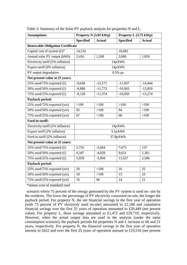
annual inflation factor. The results of the payback analysis for properties N and L are

shown in Figure 3 and Figure 4, respectively. A summary of the different analysis

scenarios is provided in Table 3. When using the specified output data, the shortest

payback period for properties N and L is 16 years and 14 years, respectively, under a

Figure 3: Solar PV payback periods for property N (3.02 kWp) based on specified and

actual performance, different electricity consumption scenarios and feed-in-tariffs

Figure 4: Solar PV payback periods for property L (3.75kWp) based on specified and

actual performance, different electricity consumption scenarios and feed-in-tariffs

-£20,000

-£10,000

£0

£10,000

£20,000

£30,000

0 10 20 30 40 50 60 70 80 90 100

Cu

mu

lati

ve d

isco

un

ted

cas

hfl

ow

Year

75% used / 25% export (specified) 75% used / 25% export (actual)

50% used / 50% export (specified) 50% used / 50% export (actual)

25% used / 75% export (specified) 25% used / 75% export (actual)

-£30,000

-£20,000

-£10,000

£0

£10,000

£20,000

£30,000

0 10 20 30 40 50 60 70 80 90 100

Cu

mu

lati

ve d

isco

un

ted

cas

hfl

ow

Year

75% used / 25% export (specified) 75% used / 25% export (actual)

50% used / 50% export (specified) 50% used / 50% export (actual)

25% used / 75% export (specified) 25% used / 75% export (actual)

Table 3: Summary of the Solar PV payback analysis for properties N and L

Assumptions Property N (3.02 kWp) Property L (3.75 kWp)

Specified Actual Specified Actual

Renewable Obligation Certificate

Capital cost of system (£)* 14,510 18,082

Annual solar PV output (kWh) 2,416 1,268 3,000 1,859

Electricity tariff (5% inflation) 14p/kWh

Export tariff (0% inflation) 14p/kWh

PV output degradation 0.5% pa

Net present value at 25 years:

25% used/75% exported (£) -9,648 -12,171 -11,937 -14,444

50% used/50% exported (£) -8,888 -11,772 -10,993 -13,859

75% used/25% exported (£) -8,128 -11,374 -10,050 -13,274

Payback period:

25% used/75% exported (yrs) >100 >100 >100 >100

50% used/50% exported (yrs) 95 >100 94 >100

75% used/25% exported (yrs) 67 >100 66 >100

Feed-in-tariff:

Electricity tariff (5% inflation) 14p/kWh

Export tariff (2% inflation) 3.1p/kWh

Feed-in tariff (2% inflation) 37.8p/kWh

Net present value at 25 years:

25% used/75% exported (£) 2,755 -5,664 7,675 137

50% used/50% exported (£) 4,347 -4,829 9,651 1,361

75% used/25% exported (£) 5,939 -3,994 11,627 2,586

Payback period:

25% used/75% exported (yrs) 20 >100 16 25

50% used/50% exported (yrs) 18 >100 15 23

75% used/25% exported (yrs) 16 66 14 21

*minus cost of standard roof

scenario where 75 percent of the energy generated by the PV system is used on- site by

the residents. The lower the percentage of PV electricity consumed on-site, the longer the

payback period. For property N, the net financial savings in the first year of operation

(with 75 percent of PV electricity used on-site) amounted to £1,186 and cumulative

financial savings over the first 25 years of operation amounted to £20,449 (net present

value). For property L, these savings amounted to £1,472 and £29,710, respectively.

However, when the actual output data are used in the analysis (under the same

consumption scenario), the payback periods for properties N and L increase to 66 and 21

years, respectively. For property N, the financial savings in the first year of operation

amount to £622 and over the first 25 years of operation amount to £10,516 (net present

value). These figures again underline the impact that under-performing PV systems can

have on payback periods.

5 Conclusion and Further Research

The introduction of feed-in tariffs in the UK has clearly transformed the economics of

solar PV systems and, in doing so, made them a much more cost-effective measure for

generating renewable energy. Based on the evidence presented here, a 3.02kWp solar PV

system performing to its design specification would have a payback period of just 16

years, under a scenario where the household is using 75% of the electricity generated on-

site. However, without the feed-in tariff, the same system would have an estimated

payback period of 67 years. This analysis underlines the importance of ensuring that

solar PV systems are functioning properly; even with feed-in tariff income, the payback

period for under-performing solar PV systems increases significantly. Further research is

required to pinpoint reasons for poor performance, whether they are technical or user

issues to ensure payback periods are minimised.

6 Acknowledgement

The authors' wish to acknowledge the financial support received from the eaga

Charitable Trust and South Yorkshire Housing Association. The contribution of

Rotherham Metropolitan Borough Council is also acknowledged.

7 References

Dunlop, E. D., Halton, D. (2006). The performance of crystalline silicon photovoltaic

solar modules after 22 years of continuous outdoor exposure, Progress in

Photovoltaics: Research and Applications, ISSN 1062-7995, 01 14, pp. 53 - 64

Banks, E. (2009), Dictionary of Finance, Investment and Banking, Palgrave Macmillan

ISBN 0230238297, P398

DECC (2009) The UK Renewable Energy Strategy, The Stationery Office, London.

Department for Communities and Local Government. (2006), Review of Sustainability

of Existing Buildings, The Energy Efficiency of Dwellings – Initial Analysis,

Product code 06 BD 04239

Department for Trade and Industry. (2006), UK Energy in Brief, DTI, London. DTI/Pub

8340/4.5k/07/06/NP. URN 06/220

Ofgem (2011) Feed-in Tariff Table 1 August 2011, www.ofgem.gov.uk

Stern, N. (2006): The Economics of Climate Change, The Stern Review, Cambridge

University Press, ISBN 0-521-70080-9, 2006